Embed Size (px)
Citation preview
Local defect correction for time-dependent problems
Minero, R.
DOI:10.6100/IR608579
Published: 01/01/2006
Document VersionPublisher’s PDF, also known as Version of Record (includes final page, issue and volume numbers)
Please check the document version of this publication:
• A submitted manuscript is the author's version of the article upon submission and before peer-review. There can be important differencesbetween the submitted version and the official published version of record. People interested in the research are advised to contact theauthor for the final version of the publication, or visit the DOI to the publisher's website.• The final author version and the galley proof are versions of the publication after peer review.• The final published version features the final layout of the paper including the volume, issue and page numbers.
Link to publication
Citation for published version (APA):Minero, R. (2006). Local defect correction for time-dependent problems Eindhoven: Technische UniversiteitEindhoven DOI: 10.6100/IR608579
General rightsCopyright and moral rights for the publications made accessible in the public portal are retained by the authors and/or other copyright ownersand it is a condition of accessing publications that users recognise and abide by the legal requirements associated with these rights.
• Users may download and print one copy of any publication from the public portal for the purpose of private study or research. • You may not further distribute the material or use it for any profit-making activity or commercial gain • You may freely distribute the URL identifying the publication in the public portal ?
Take down policyIf you believe that this document breaches copyright please contact us providing details, and we will remove access to the work immediatelyand investigate your claim.
Download date: 25. Jun. 2018
Local Defect Correctionfor Time-Dependent Problems
Copyright c©2006 by Remo Minero, Eindhoven, The Netherlands.
All rights are reserved. No part of this publication may be reproduced, stored in a
retrieval system, or transmitted, in any form or by any means, electronic, mechani-
cal, photocopying, recording or otherwise, without prior permission of the author.
CIP-DATA LIBRARY TECHNISCHE UNIVERSITEIT EINDHOVEN
Minero, Remo
Local defect correction for time-dependent problems / door Remo Minero. -
Eindhoven: Technische Universiteit Eindhoven, 2006.
Proefschrift. - ISBN 90-386-0754-7. - 978-90-386-0754-2
NUR 919
Subject headings: parabolic differential equations; numerical methods /
initial value problems; numerical methods
2000 Mathematics Subject Classification: 65M50, 65M06, 76F25
Local Defect Correctionfor Time-Dependent Problems
PROEFSCHRIFT
ter verkrijging van de graad van doctor aan de
Technische Universiteit Eindhoven, op gezag van de
Rector Magnificus, prof.dr.ir. C.J. van Duijn, voor een
commissie aangewezen door het College
voor Promoties in het openbaar te verdedigen
op donderdag 1 juni 2006 om 16.00 uur
door
Remo Minero
geboren te Borgosesia, Italie
Dit proefschrift is goedgekeurd door de promotor:
prof.dr. R.M.M. Mattheij
Copromotor:
dr.ir. M.J.H. Anthonissen
This project was funded by NWO (Netherlands
Organisation for Scientific Research) under the
research program Computational Science, grant
number 635.000.002

To Lidia

Contents
1 Introduction 1
1.1 Transport of passive tracers . . . . . . . . . . . . . . . . . . . . . . . . . 1
1.1.1 Adaptive grid methods for time-dependent problems . . . . . . 2
1.2 The LDC method for elliptic problems . . . . . . . . . . . . . . . . . . . 4
1.3 Outline of this thesis . . . . . . . . . . . . . . . . . . . . . . . . . . . . . 7
2 The LDC method for parabolic partial differential equations 9
2.1 Performing one time step with LDC . . . . . . . . . . . . . . . . . . . . 10
2.1.1 A composite grid solution at time tn . . . . . . . . . . . . . . . . 11
2.1.2 The defect correction . . . . . . . . . . . . . . . . . . . . . . . . . 13
2.1.3 Properties of the LDC time step . . . . . . . . . . . . . . . . . . . 15
2.2 The LDC algorithm including regridding . . . . . . . . . . . . . . . . . 18
2.3 Numerical experiments . . . . . . . . . . . . . . . . . . . . . . . . . . . . 22
2.3.1 Example 1: a 2D convection-diffusion problem . . . . . . . . . . 23
2.3.2 Example 2: comparison between LDC and LUGR . . . . . . . . 26
3 Convergence properties of LDC 31
3.1 The iteration matrix . . . . . . . . . . . . . . . . . . . . . . . . . . . . . 32
3.2 A one-dimensional model problem . . . . . . . . . . . . . . . . . . . . . 34
3.2.1 Bounds for the M1 infinity norm . . . . . . . . . . . . . . . . . . 35
3.2.2 The expression of the M2 infinity norm . . . . . . . . . . . . . . 37
3.3 Iteration matrix norm asymptotics . . . . . . . . . . . . . . . . . . . . . 40
3.3.1 The limit for small values of the time step ∆t . . . . . . . . . . . 40
3.3.2 The stationary case limit . . . . . . . . . . . . . . . . . . . . . . . 46
3.3.3 Plots of the iteration matrix norm . . . . . . . . . . . . . . . . . 47
3.4 One-dimensional numerical experiments . . . . . . . . . . . . . . . . . 49
3.5 Two-dimensional numerical experiments . . . . . . . . . . . . . . . . . 53
4 A finite volume adapted LDC method 59
4.1 Problem formulation and initialization of LDC . . . . . . . . . . . . . . 60
4.1.1 Composite grid definition . . . . . . . . . . . . . . . . . . . . . . 61
4.1.2 Computation of a composite grid solution . . . . . . . . . . . . . 64
viii Contents
4.2 The finite volume adapted defect term . . . . . . . . . . . . . . . . . . . 66
4.2.1 Approximation of the defect . . . . . . . . . . . . . . . . . . . . . 68
4.2.2 The finite volume adapted LDC algorithm . . . . . . . . . . . . . 71
4.2.3 Practical considerations on the defect term . . . . . . . . . . . . 73
4.3 Conservation properties of LDC . . . . . . . . . . . . . . . . . . . . . . . 76
4.4 Numerical experiments . . . . . . . . . . . . . . . . . . . . . . . . . . . . 79
4.4.1 Example 1: comparison with a uniform grid solver . . . . . . . . 79
4.4.2 Example 2: comparison with the standard LDC method . . . . . 82
5 Generalizations of the LDC method 85
5.1 A conservative regridding strategy . . . . . . . . . . . . . . . . . . . . . 85
5.1.1 Providing initial values on the new composite grid . . . . . . . . 87
5.1.2 A numerical example . . . . . . . . . . . . . . . . . . . . . . . . . 91
5.2 LDC algorithm with multiple levels of refinements . . . . . . . . . . . . 93
6 Solving transport problems using LDC 97
6.1 Mathematical model . . . . . . . . . . . . . . . . . . . . . . . . . . . . . 98
6.2 Numerical method . . . . . . . . . . . . . . . . . . . . . . . . . . . . . . . 100
6.2.1 Implementation . . . . . . . . . . . . . . . . . . . . . . . . . . . . 103
6.3 Numerical results . . . . . . . . . . . . . . . . . . . . . . . . . . . . . . . 103
6.3.1 Comparison between LDC and the spectral method . . . . . . . 107
7 Conclusions and recommendations 113
Bibliography 115
Index 121
Summary 123
Samenvatting (Summary in Dutch) 125
Acknowledgements 127
Curriculum vitae 129
Chapter 1
Introduction
1.1 Transport of passive tracers
In everyday life we often see the dispersion in the atmosphere of exhaust gases
from a chimney, or the dispersion of the smoke produced by a cigarette. These are
examples of tracer transport in given velocity fields. The flow field is given by the
movement of the air in the atmosphere, while the tracer is represented by the mix-
ture of heated gas and suspended particles that are injected in the air. The tracer is
called passive when its concentration is so low that the main flow dynamics is not
influenced by the presence of the external particles. An environmental example of
passive tracer transport is the dispersion of dye or pollutants in a river or in the sea.
The same kind of phenomenon occurs in many engineering applications; examples
are the transport of fly ashes in burners or the turbulent mixing in chemical reac-
tors. In order to efficiently design this type of machines, it is important to unravel
the influence of the turbulent flow on the transport mechanism. In the case of chem-
ical reactors, in fact, turbulence can positively affect mixing of chemical species, and
hence facilitate their reaction.
Mathematically the transport process is modeled by a time-dependent advection-
diffusion equation. In turbulent flows, passive scalar transport is characterized by
a length scale that can be significantly smaller than the size of the turbulent eddies
in the main flow [26]. From a computational point of view this means that even
a higher resolution is needed to simulate the transport process than required for
the turbulence itself. This implies that a proper description of the transport phe-
nomena is computationally more expensive than running Direct Numerical Simu-
lations (DNS) of turbulence. However, in many practical applications filaments of
tracer material are mainly confined in a limited part of the computational domain.
In other words, the solution of the advection-diffusion equation that models the
2 Chapter 1 - Introduction
transport process is often characterized by local regions of high activity, i.e. regions
where spatial gradients are quite large compared to those in the rest of the domain,
where the solution presents a relatively smooth behavior. Examples of solutions of
Partial Differential Equations (PDEs) exhibiting local regions of high activity are
frequently encountered also in many other areas, like shock hydrodynamics, com-
bustion, etc.
An efficient numerical solution of this kind of problems requires the usage of adap-
tive grid techniques. In adaptive grid methods, a fine grid spacing and possibly a
small time step are adopted only where the large variations occur, so that the com-
putational effort and the memory requirements are minimized.
1.1.1 Adaptive grid methods for time-dependent problems
A large number of adaptive grid methods for time-dependent problems have been
proposed in the literature. A first category includes the moving-grid or dynamic-
regridding methods. In this approach, nodes are moving continuously in the space-
time domain, like in classical Lagrangian methods, and the discretization of the
PDEs is coupled with the motion of the grid. Methods in this category differ in
how the motion of the grid is governed. The grid is anyhow always nonuniform and
the number of nodes remains constant in time. The nonuniformity of the grid im-
plies that programming these methods often involves quite complicated data struc-
tures. An example of a dynamic-regridding technique is the moving mesh strat-
egy (MMPDE) introduced in [36] for one-dimensional problems and then extended
to 2D in [37]. In MMPDE the physical PDE is solved together with a partial dif-
ferential equation that describes the movement of the mesh. Practical issues about
MMPDE are addressed in [35]; these include a proper control of the mesh concen-
tration by means of monitor functions. In [8, 9] it is shown that the monitor func-
tions strongly influence the accuracy of the computation; moreover algorithms in
which the physical PDE is decoupled from the mesh equation are proposed. In [68]
an adaptive moving mesh technique for reaction-diffusion equation is described; in
this case the movement of the mesh is determined by minimizing an energy func-
tional, the so-called mesh-energy integral, which is defined from certain monitor
functions. In [58] a conservative-interpolation formula is introduced to guarantee
discrete mass conservation in the numerical solution when the mesh is moved.
Another type of adaptive grid techniques is represented by static-regridding meth-
ods. Here, the idea is to adapt the grid at each time step by adding grid points where
a high activity occurs and removing them where they are no longer needed. This
process is controlled by error estimates or methods based on the measure of some
characteristics of the solution (e.g. gradients, slope, etc.). In this kind of methods
the number of grid points is not constant in time. An example of a static-regridding
strategy is the Adaptive Mesh Refinement (AMR) technique introduced in [12, 14]
for the solution of hyperbolic PDEs. In AMR a global coarse grid covers the whole
domain, and finer and finer grids are added locally to resolve the high variations of
1.1 Transport of passive tracers 3
the solution till the required level of accuracy is reached. In [14] the rectangular
subgrids may be skewed with respect to the global rectangular domain axes: this is
to allow alignment of the local grids with the steep regions of the solution. In [12]
the focus is on discrete conservation and the boundaries of the nested grids coincide
with grid lines of the underlying coarse mesh; time integration is performed explic-
itly. More recent variants and applications of AMR can be found in [13, 31, 50].
Another example of a static-regridding technique is the Local Uniform Grid Refine-
ment (LUGR) method, described and analyzed in [60, 62–64]. LUGR is proposed
for the solution of parabolic PDEs and in this method time integration is generally
performed implicitly. LUGR is applied to the solution of transport problems in het-
erogeneous porous media in [61], while an LUGR based strategy for electrochemical
applications is introduced in [15]. Implementation and algorithmic issues of LUGR
are discussed in [16]. Briefly, the method works as follows: at each time step the
PDE is first integrated on a global uniform coarse grid. The coarse grid solution at
the new time step provides artificial boundary conditions on a local uniform fine grid
and the problem is then solved locally with a smaller time step than the one used
on the global grid. At this point, the fine grid values are used to replace the coarse
grid values in the region of refinement. The procedure can be repeated recursively
to include more levels of refinement. The technique relies on the fact that the coarse
grid solution provides artificial boundary conditions for the local problem that are
accurate enough. The main advantage of LUGR is the possibility of working with
uniform grids and uniform grid solvers only.
A drawback of static-regridding methods against moving-grid methods is that they
generally use more nodes to obtain a given accuracy. However, in moving-grid meth-
ods special care must be taken in order to prevent grid distortion; this occurs for ex-
ample when vertex angles become too close to 0 or 180 in triangular meshes. This
phenomenon can reduce the accuracy of the computations considerably. As a conse-
quence moving-grid methods require more parameter tuning than static-regridding
techniques.
This thesis focuses on a new static-regridding technique for time-dependent prob-
lems: Local Defect Correction (LDC). LDC shares with LUGR the possibility and
the advantage of working with uniform grids and uniform grid solvers only. In LDC,
however, the fine grid solution at the new time step is used not only to replace the
coarse grid values in the area of refinement, but to overall improve the coarse grid
approximation. This can be achieved through a defect correction, in which the fine
grid solution is used to approximate the coarse grid local discretization error. The
improved coarse grid approximation defines new artificial boundary conditions for a
new local problem, which in turn can correct the solution globally. In this way, LDC
does not have to rely on the accuracy of the artificial boundary condition provided
by the first coarse grid approximation, turning out to be a more robust technique
than LUGR. The method we introduce in this thesis is a generalization of the local
defect correction method developed for the efficient solution of elliptic PDEs.
4 Chapter 1 - Introduction
1.2 The LDC method for elliptic problems
As a technique for solving elliptic problems with highly localized properties, local
defect correction was initially presented in [34]. LDC is an iterative procedure
in which the elliptic problem is first solved on a global coarse grid (grid size H).
This first coarse grid approximation provides, via interpolation, artificial Dirichlet
boundary conditions to a local fine grid (grid size h < H); the fine grid is located
where the high activity in the solution occurs. A discrete boundary value problem is
now solved locally. The local solution is then plugged into the coarse grid discretiza-
tion scheme in order to get an approximation of the coarse grid local discretization
error or defect. The defect, added to the right hand side of the coarse grid problem,
leads to determining a more accurate coarse grid approximation. This provides up-
dated boundary conditions for a new local problem, whose solution will be used to
further improve the approximation globally. The entire procedure can be repeated
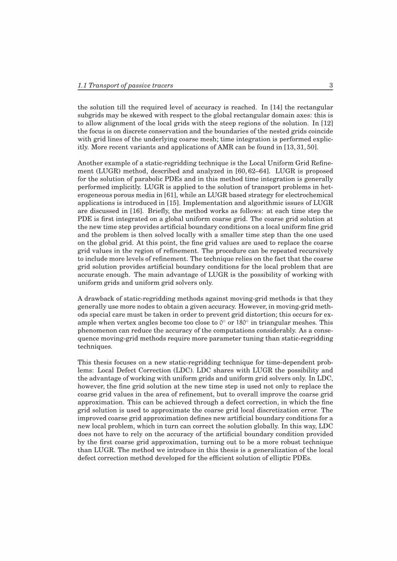
until a fixed point in the iteration is reached. The scheme of the LDC iteration is
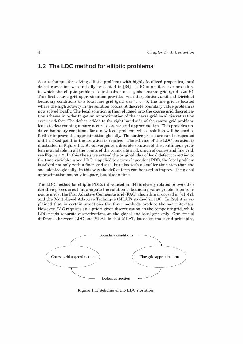
illustrated in Figure 1.1. At convergence a discrete solution of the continuous prob-
lem is available in all the points of the composite grid, union of coarse and fine grid,
see Figure 1.2. In this thesis we extend the original idea of local defect correction to
the time variable: when LDC is applied to a time-dependent PDE, the local problem
is solved not only with a finer grid size, but also with a smaller time step than the
one adopted globally. In this way the defect term can be used to improve the global
approximation not only in space, but also in time.
The LDC method for elliptic PDEs introduced in [34] is closely related to two other
iterative procedures that compute the solution of boundary value problems on com-
posite grids: the Fast Adaptive Composite grid (FAC) algorithm proposed in [41, 42],
and the Multi-Level Adaptive Technique (MLAT) studied in [18]. In [28] it is ex-
plained that in certain situations the three methods produce the same iterates.
However, FAC requires an a priori given discretization on the composite grid, while
LDC needs separate discretizations on the global and local grid only. One crucial
difference between LDC and MLAT is that MLAT, based on multigrid principles,
Defect correction
Fine grid approximationCoarse grid approximation
Boundary conditions
Figure 1.1: Scheme of the LDC iteration.
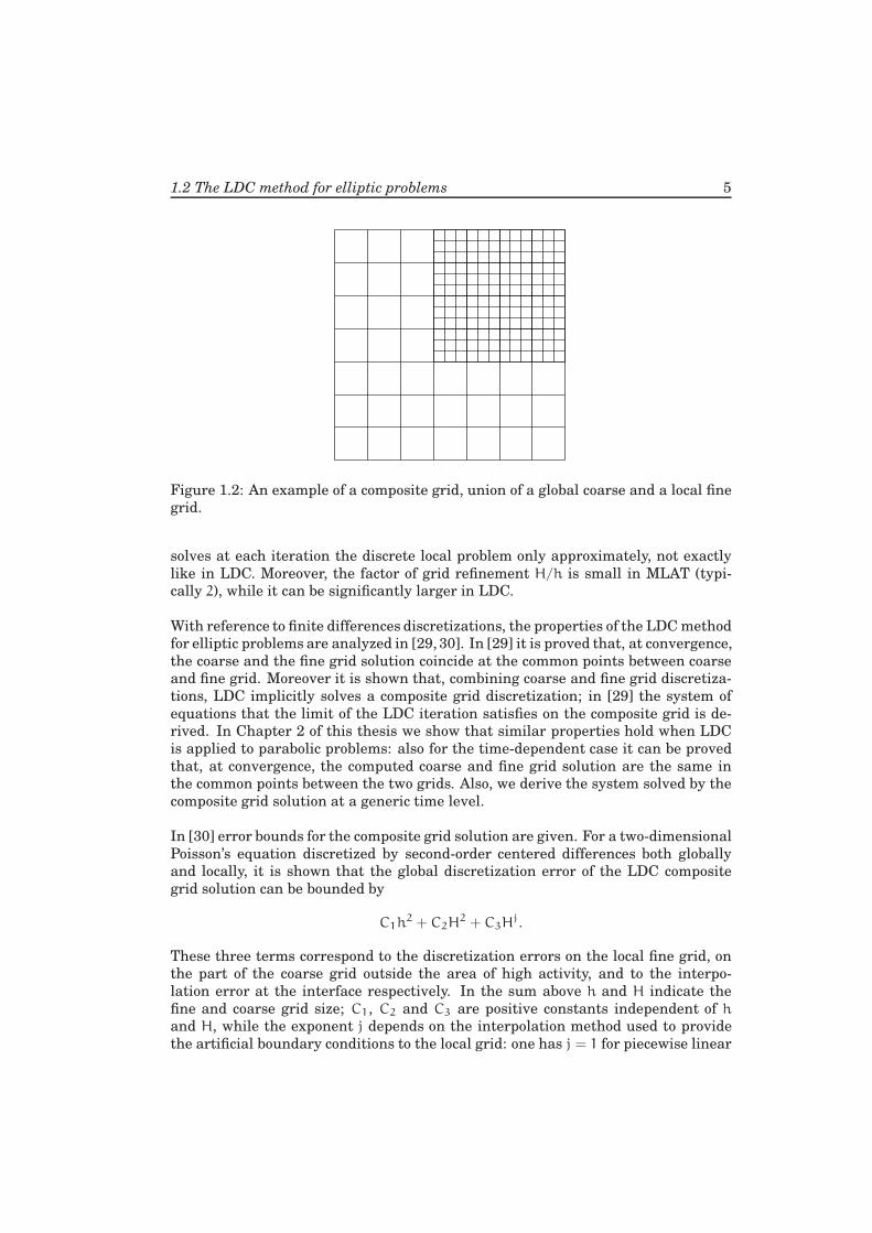
1.2 The LDC method for elliptic problems 5
Figure 1.2: An example of a composite grid, union of a global coarse and a local fine
grid.
solves at each iteration the discrete local problem only approximately, not exactly
like in LDC. Moreover, the factor of grid refinement H/h is small in MLAT (typi-
cally 2), while it can be significantly larger in LDC.
With reference to finite differences discretizations, the properties of the LDC method
for elliptic problems are analyzed in [29, 30]. In [29] it is proved that, at convergence,
the coarse and the fine grid solution coincide at the common points between coarse
and fine grid. Moreover it is shown that, combining coarse and fine grid discretiza-
tions, LDC implicitly solves a composite grid discretization; in [29] the system of
equations that the limit of the LDC iteration satisfies on the composite grid is de-
rived. In Chapter 2 of this thesis we show that similar properties hold when LDC
is applied to parabolic problems: also for the time-dependent case it can be proved
that, at convergence, the computed coarse and fine grid solution are the same in
the common points between the two grids. Also, we derive the system solved by the
composite grid solution at a generic time level.
In [30] error bounds for the composite grid solution are given. For a two-dimensional
Poisson’s equation discretized by second-order centered differences both globally
and locally, it is shown that the global discretization error of the LDC composite
grid solution can be bounded by
C1h2 + C2H
2 + C3Hj.
These three terms correspond to the discretization errors on the local fine grid, on
the part of the coarse grid outside the area of high activity, and to the interpo-
lation error at the interface respectively. In the sum above h and H indicate the
fine and coarse grid size; C1, C2 and C3 are positive constants independent of h
and H, while the exponent j depends on the interpolation method used to provide
the artificial boundary conditions to the local grid: one has j = 1 for piecewise linear
6 Chapter 1 - Introduction
interpolation, j = 2 for piecewise quadratic interpolation. The terms C1, C2 and C3
measure the continuous solution’s smoothness in the area of refinement, outside the
area of refinement and along the interface between coarse and fine grid respectively.
Since the solution of the Poisson’s equation is assumed to have a high activity in the
area of refinement, one typically has C1 ≫ C2; this can be balanced by choosing
h2 ≪ H2. Experimental evidence (see again [30] and also [28]) shows that C3 is
generally much smaller than C1 and C2.
The convergence behavior of the LDC method for elliptic problems is analyzed in [4].
The LDC iteration is expressed in terms of an iteration matrix, whose properties are
studied analytically and experimentally for the two-dimensional Poisson’s equation
discretized by finite differences. In general, it is observed that LDC converges very
fast and that iteration errors are reduced by several orders of magnitude at each
iteration step. In Chapter 3 of this thesis we use a similar approach to study the
convergence properties of the LDC method for parabolic problems. Also for the time-
dependent case we find that LDC converges very fast and that, in practice, only very
few iterations per time step are required for convergence.
In LDC one is not forced to use finite difference discretizations. In [66], for instance,
local defect correction is combined with the finite element method, while a finite
volume adapted LDC algorithm that guarantees discrete conservation on the com-
posite grid is proposed in [6]. The idea in [6] is to write the defect term in such a way
that coarse and fine grid fluxes balance across the interface between coarse and fine
grid. In Chapter 4 of this thesis we extend that idea, and we apply it to parabolic
problems that are integrated on the global and on the local grid with different time
steps.
The LDC method for elliptic problems has also been employed with different grid
types. This is particularly convenient when the solution has a special symmetry [47]
or the local high activity is not aligned with global domain axes [3, 32, 33]. In [47] the
global coarse grid is Cartesian, while the local domain has a circular shape and polar
coordinates are used locally. In [33] the local fine grid is in a slantwise direction.
In [32] LDC is applied to solve combustion problems and curvilinear coordinates
are adopted locally in order to follow the shape of the flame front. In [3] similar
applications are considered, and the classical LDC algorithm is extended to include
multiple levels of refinement, domain decomposition and regridding. In a recent
paper [54] local defect correction is finally combined with high order compact finite
difference schemes for the solution of both one- and two-dimensional boundary value
problems.
To summarize, LDC has been proved to be an efficient method for solving elliptic
problems on composite grids. It has very good convergence properties, and it can be
applied for a wide range of physical problems with several discretization techniques.
In this thesis we extend the LDC principles to the solution of parabolic PDEs.
1.3 Outline of this thesis 7
1.3 Outline of this thesis
In Chapter 2 of this thesis the LDC method for parabolic problems is presented. At
each time step the PDE is integrated both on a global and on a local grid, and the two
solutions at the new time level are iteratively combined to ultimately give a solution
on the composite grid. In the method we propose, time integration on the local grid
is performed with a smaller time step than the one adopted globally. In this way, the
local solution is used to correct not only the errors in the global approximation due
to the spatial discretization, but also due to the temporal discretization. In practice
the method is such that a fine grid spacing and a small time step are adopted to
resolve the local high activity only, while a larger grid spacing and time step are
chosen globally. This implies that the global approximation at the new time level
is interpolated not only in space, but also in time, in order to compute the artificial
boundary conditions for the local problem.
In the same chapter we also illustrate some properties of the LDC time step. First,
we show that the converged coarse and fine grid solution at the new time step co-
incide at the common points between the two grids. Secondly, we derive the system
of equations that the converged LDC solution implicitly satisfies on the composite
grid. Clearly, these properties generalize the theorems proved in [29] for station-
ary LDC. Furthermore, our method takes into account that the local high activity
might move and be located in different parts of the global domain at different times.
Therefore the LDC algorithm for time-dependent problems includes a regridding
strategy: the first coarse grid solution at the new time level indicates where the
high variations at that time level occur, and the local grid is chosen accordingly. The
algorithm is tested in some concrete examples that illustrate its accuracy, efficiency
and robustness.
Chapter 3 of this thesis is devoted to the analysis of the convergence behavior of the
LDC algorithm introduced in Chapter 2. The LDC iteration that takes place at a
generic time step is expressed in terms of an iteration matrix, which is a generaliza-
tion of the expression derived in [4] for stationary cases. For one-dimensional diffu-
sion problems, the properties of the iteration matrix are studied analytically, while
for one- and two-dimensional convection-diffusion problems the analysis is carried
out experimentally. In general we observe that LDC converges for any choice of the
discretization parameters and that iteration errors are reduced by several orders of
magnitude at each iteration step.
When the new and fast converging LDC method for parabolic problems is applied
in combination with the finite volume method, the resulting numerical solution is
not necessarily conservative on the composite grid. In Chapter 4 of this thesis we
present a finite volume adapted LDC algorithm for parabolic problems that guar-
antees balance of coarse and fine grid fluxes across the interface between the global
and local grid at each time step. In this way the computed numerical solution sat-
isfies a discrete system of conservation laws on the composite grid. This system
8 Chapter 1 - Introduction
of equations is explicitly derived in Chapter 4, and the features of the method are
tested experimentally in two examples: the first one illustrates the superior effi-
ciency of the new method with respect to a uniform global fine grid solver, and the
second demonstrates discrete conservation. Our method generalizes the technique
introduced in [6] for elliptic problems.
One limitation of the finite volume adapted LDC algorithm introduced in Chapter 4
is that it can only handle fixed grids. In practice it is of interest only for those physi-
cal problems in which the high activity remains confined in the same limited part of
the global domain at all time levels. In Chapter 5 we overcome this limitation and
we incorporate a conservative regridding strategy in the finite volume adapted LDC
algorithm. Also, we extend the algorithm to include multiple levels of refinement.
The local defect correction iteration is initially applied between a global coarse grid
(level 0) and a local fine grid (level 1); when this iteration has converged, a new it-
eration takes place between level 1 and a finer grid at level 2, and so on. The time
marching strategy is such that time integration at the finer levels can be performed
with smaller time steps.
At the end (Chapter 6), the new, multilevel, conservative and fast converging LDC
method is applied to solve realistic time-dependent problems. In particular, we con-
sider the transport of passive tracers in transient flow fields. Results of numerical
simulations show that LDC produces accurate results and that it is a very promising
tool to solve also more general physical problems characterized by highly localized
properties.
In Chapter 7 we finally draw some conclusions and give recommendations for future
research.
Chapter 2
The LDC method for parabolicpartial differential equations
In this chapter we introduce the local defect correction method for solving parabolic
differential equations with highly localized properties. The method is a generaliza-
tion of the LDC technique for elliptic problems described and analyzed in [1, 29, 30,
34]. In a time-dependent setting LDC works as follows: first a time step is per-
formed on a global coarse grid. The global solution at the new time level provides
artificial boundary conditions on a local fine grid, which is adaptively placed where
the high activity occurs. A solution is then computed locally, possibly with a smaller
time step than the one adopted globally. At this point the local approximation pro-
vides an estimate for the coarse grid local discretization error or defect. The defect,
added to the right hand side of the coarse grid problem, leads to determining a more
accurate (both in space and time) global approximation of the solution. This can now
be used to update the boundary conditions locally and the entire procedure can be
repeated again until convergence. In practice, at each time step a global and a local
approximation progressively improve each other to ultimately compute a solution
on the composite grid, union of coarse and fine grid.
In comparison with other strategies for grid refinement, one of the main advantages
of the method is that the global and the local grid can always be uniform struc-
tured grids. With this respect LDC is similar to the Local Uniform Grid Refinement
(LUGR) method presented and analyzed in [60, 62–64]. LDC, however, differs from
LUGR because in LUGR the local solution does not improve the solution globally
through the defect correction. In LUGR the local solution is only used to replace
the coarse grid values in the area of refinement, while in LDC the local solution
improves the coarse grid approximation overall. In addition, LUGR relies on the
fact that the boundary conditions provided by the coarse grid approximation are
accurate enough, while in LDC also the artificial boundary conditions are progres-
10 Chapter 2 - The LDC method for parabolic partial differential equations
sively improved. For these reasons it turns out that LDC is a more robust technique
than LUGR.
This chapter is based on the research results previously presented in [43, 44].
2.1 Performing one time step with LDC
In this section we describe the LDC time step for a parabolic problem. We assume
a solution to be known on the composite grid at a certain time level and we explain
how to compute a solution on the composite grid at the next time level by means
of LDC.
We consider the following two-dimensional problem
∂u(x, t)
∂t= Lu(x, t) + f(x, t), in Ω×Θ,
u(x, t) = ψ(x, t), on ∂Ω×Θ,
u(x, 0) = ϕ0(x), in Ω,
(2.1)
where Ω is a spatial domain, ∂Ω its boundary and Ω := Ω ∪ ∂Ω. Moreover, Θ is
the time interval (0, tend], L a linear elliptic operator, f a source term, ψ a Dirichlet
boundary condition and ϕ0 a given initial condition. For ease of presentation we
only consider Dirichlet boundary conditions. However this is not restrictive and the
implementation of other types of boundary conditions (e.g. Neumann or Robin) is
straightforward. We assume that u has a region of high activity that covers a small
part of Ω.
Problem (2.1) is discretized in space and time in order to be solved numerically. For
that, inΩ we introduce the global uniform coarse grid (grid size H)ΩH and the time
step ∆t. Grid points ∂ΩH are placed on ∂Ω too and we define ΩH := ΩH ∪ ∂ΩH.
Because of the high activity of the solution, at time tn := n∆t a coarse grid ap-
proximation computed with a time step ∆t might be not adequate enough to rep-
resent u(x, tn). In order to better capture the local high activity, we also solve the
problem on the local domain Ωnl ⊂ Ω. We denote the boundary of Ωn
l by ∂Ωnl
and we define Ωnl := Ωn
l ∪ ∂Ωnl . In Ωn
l the superscript n refers to the time level.
This is needed because the area of refinement is updated at each time step to adap-
tively follow the behavior of the solution. This is discussed in Section 2.2. Here we
just assume the local domain to be given and placed where the area of high activ-
ity at time tn occurs. On the local domain we introduce a uniform fine grid (grid
size h < H), which we denote by Ωh,nl . Grid points ∂Ωh,n
l are also placed on ∂Ωnl
and we define Ωh,nl := Ωh,n
l ∪ ∂Ωh,nl . The region of refinement and the fine grid
spacing h are chosen is such a way that coarse grid points that lie in the area of
refinement belong to the fine grid too. On Ωh,nl the time integration is performed
2.1 Performing one time step with LDC 11
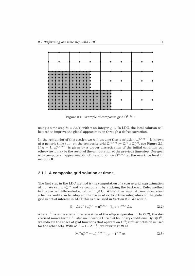
Figure 2.1: Example of composite grid ΩH,h,n.
using a time step δt = ∆t/τ, with τ an integer ≥ 1. In LDC, the local solution will
be used to improve the global approximation through a defect correction.
In the remainder of this section we will assume that a solution uH,h,n−1∗
is known
at a generic time tn−1 on the composite grid ΩH,h,n := ΩH ∪ Ωh,nl , see Figure 2.1.
If n = 1, uH,h,n−1∗
is given by a proper discretization of the initial condition ϕ0,
otherwise it may be the result of the computation of the previous time step. Our goal
is to compute an approximation of the solution on ΩH,h,n at the new time level tnusing LDC.
2.1.1 A composite grid solution at time tn
The first step in the LDC method is the computation of a coarse grid approximation
at tn. We call it uH,n0 and we compute it by applying the backward Euler method
to the partial differential equation in (2.1). While other implicit time integration
schemes could also be adopted, the usage of explicit time integrators on the global
grid is not of interest in LDC; this is discussed in Section 2.2. We obtain
(I− ∆t LH)uH,n0 = uH,h,n−1
∗|ΩH + fH,n∆t, (2.2)
where LH is some spatial discretization of the elliptic operator L. In (2.2), the dis-
cretized source term fH,n also includes the Dirichlet boundary conditions. By G(ΩH)
we indicate the space of grid functions that operate on ΩH; similar notation is used
for the other sets. With MH := I− ∆t LH, we rewrite (2.2) as
MHuH,n0 = uH,h,n−1
∗|ΩH + fH,n∆t. (2.3)
12 Chapter 2 - The LDC method for parabolic partial differential equations
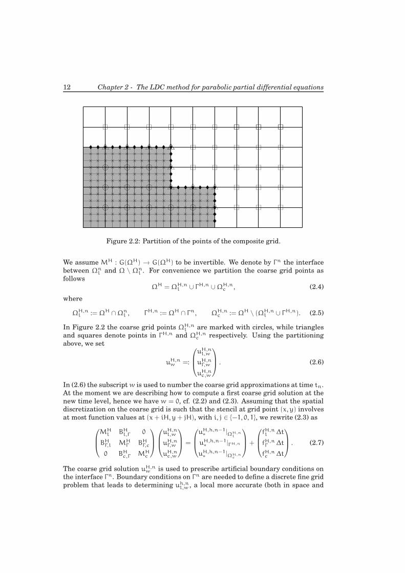
Figure 2.2: Partition of the points of the composite grid.
We assume MH : G(ΩH) → G(ΩH) to be invertible. We denote by Γn the interface
between Ωnl and Ω \ Ωn
l . For convenience we partition the coarse grid points as
follows
ΩH = ΩH,nl ∪ ΓH,n ∪ΩH,n
c , (2.4)
where
ΩH,nl := ΩH ∩Ωn
l , ΓH,n := ΩH ∩ Γn, ΩH,nc := ΩH \ (ΩH,n
l ∪ ΓH,n). (2.5)
In Figure 2.2 the coarse grid points ΩH,nl are marked with circles, while triangles
and squares denote points in ΓH,n and ΩH,nc respectively. Using the partitioning
above, we set
uH,nw =:
uH,nl,w
uH,nΓ,w
uH,nc,w
. (2.6)
In (2.6) the subscriptw is used to number the coarse grid approximations at time tn.
At the moment we are describing how to compute a first coarse grid solution at the
new time level, hence we have w = 0, cf. (2.2) and (2.3). Assuming that the spatial
discretization on the coarse grid is such that the stencil at grid point (x, y) involves
at most function values at (x+ iH, y+ jH), with i, j ∈ −1, 0, 1, we rewrite (2.3) as
MHl BH
l,Γ 0
BHΓ,l MH
Γ BHΓ,c
0 BHc,Γ MH
c
uH,nl,w
uH,nΓ,w
uH,nc,w
=
uH,h,n−1∗
|ΩH,nl
uH,h,n−1∗
|ΓH,n
uH,h,n−1∗
|ΩH,nc
+
fH,nl ∆t
fH,nΓ ∆t
fH,nc ∆t
. (2.7)
The coarse grid solution uH,nw is used to prescribe artificial boundary conditions on
the interface Γn. Boundary conditions on Γn are needed to define a discrete fine grid
problem that leads to determining uh,nl,w , a local more accurate (both in space and
2.1 Performing one time step with LDC 13
time) approximation of u(tn). We can prescribe artificial Dirichlet boundary condi-
tions at tn by applying an interpolation operator in space Ph,H : G(ΓH,n)→ G(Γh,n)
to uH,nw ; by Γh,n we denoted the set of fine grid points that lie on the interface Γn.
In Figure 2.2 the points Γh,n are marked with small diamonds. In LDC the oper-
ator Ph,H generally performs piecewise linear or piecewise quadratic interpolation
(cf. [30]). If we want to perform time integration with a time step δt = ∆t/τ, we
also need to provide boundary conditions on Γh,n at all the intermediate time lev-
els tn−1+k/τ, with k = 1, 2, . . . , τ− 1. Therefore we perform linear time interpolation
between uH,h,n−1∗
|Γh,n and Ph,HuH,nw . Note that in order to solve the problem locally
on Ωnl we have to specify boundary conditions not only on Γh,n ⊂ ∂Ωh,n
l , but on the
whole ∂Ωh,nl . However, for the fine grid points ∂Ωh,n
l \ Γh,n we can use a proper
discretization of the boundary condition for the continuous problem (2.1). We let Lhl
be a local fine grid discretization of the operator L and we introduceMhl := I− δt Lh
l .
A first fine grid approximation (w = 0) at time tn can thus be computed solving
Mhl u
h,n−1+k/τ
l,w = uh,n−1+(k−1)/τ
l,w + fh,n−1+k/τ
l δt
− Bhl,Γ
(
k
τPh,HuH,n
Γ,w +τ − k
τuH,h,n−1∗
|Γh,n
)
, for k = 1, 2, . . . , τ. (2.8)
In (2.8) the fine grid discretized source term fh,n−1+k/τ
l also includes the boundary
conditions for the fine grid points ∂Ωh,nl \ Γh,n. The procedure (2.8) is initialized
using
uh,n−1l,w = uH,h,n−1
∗|Ωh,n
l. (2.9)
We combine all the equations in (2.8) to express the fine grid approximation uh,nl,w
directly in terms of uH,h,n−1∗
|Ωh,nl
. We obtain
(
Mhl
)τuh,n
l,w = uH,h,n−1∗
|Ωh,nl
+
τ∑
k=1
(
Mhl
)k−1fh,n−1+k/τ
l δt
−
τ∑
k=1
(
Mhl
)k−1Bh
l,Γ
(
k
τPh,HuH,n
Γ,w +τ− k
τuH,h,n−1∗
|Γh,n
)
, (2.10)
or
(
Mhl
)τuh,n
l,w = uH,h,n−1∗
|Ωh,nl
+ Fh,nl δt−Wn
l,ΓPh,HuH,n
Γ,w + Znl,Γu
H,h,n−1∗
|Γh,n . (2.11)
In (2.11) Fh,nl depends only on the source term and on the fine grid operator Mh
l ,
while Wnl,Γ and Zn
l,Γ only depend on Mhl and Bh
l,Γ .
2.1.2 The defect correction
The crucial part of the LDC method is how the local solution uh,nl,w is used to improve
the global approximation uH,nw through an approximation of the coarse grid local
14 Chapter 2 - The LDC method for parabolic partial differential equations
discretization error or defect. The defect dH,n is defined as
dH,n := MH u(tn)|ΩH − u(tn−1)|ΩH − fH,n∆t. (2.12)
In (2.12) we substituted the projection on ΩH of the continuous solution u into the
discretization scheme (2.3). If we would know the values of the defect dH,n, we
could use them to find a better approximation of un on the coarse grid. This could
be achieved by adding dH,n to the right hand side of (2.3). However, since we do not
know the exact solution of our partial differential equation, we cannot compute the
values of dH,n. What we can do, though, is to use the more accurate local approxi-
mation uh,nl to get a local estimate dH,n
l of dH,n. The local estimate of the defect is
computed on ΩHl plugging the fine grid solution into the coarse grid discretization
scheme in that region. We obtain (cf. the first equation in (2.7))
dH,nl,w−1 :=MH
l RH,huh,n
l,w−1 + BHl,Γu
H,nΓ,w−1 − uH,h,n−1
∗|ΩH
l− fH,n
l ∆t, (2.13)
where RH,h : G(Ωh,nl )→ G(ΩH,n
l ) is a restriction operator from the fine to the coarse
grid, such that
(RH,huh,nl,w−1)(x, y) = uh,n
l,w−1(x, y), ∀(x, y) ∈ ΩH,nl . (2.14)
The defect dH,nl,w−1 is now added to the right hand side of (2.7). A more accurate
coarse grid approximation is thus computed solving
MHuH,nw =
uH,h,n−1∗
|ΩH,nl
uH,h,n−1∗
|ΓH,n
uH,h,n−1∗
|ΩH,nc
+
fH,nl ∆t+ dH,n
l,w−1
fH,nΓ ∆t
fH,nc ∆t
=
0
uH,h,n−1∗
|ΓH,n
uH,h,n−1∗
|ΩH,nc
+
MHl R
H,huh,nl,w−1 + BH
l,ΓuH,nΓ,w−1
fH,nΓ ∆t
fH,nc ∆t
.
(2.15)
The new coarse grid solution can be used to update the boundary conditions for a
new local problem onΩh,nl , which in turn will correct the coarse grid approximation.
This defines the LDC iteration process, cf. Figure 1.1.
We note that, as discussed in [4, 27, 34, 66] for LDC in stationary problems, some-
times it might be convenient to compute dH,nl,w−1 not at all points of ΩH,n
l , but in a
subset ΩHdef only. In particular, points lying close to the interface Γn should be ex-
cluded. In this way points of Γn and points ofΩHdef are separated by a so-called safety
region . Figure 2.3 shows an example of a composite grid without a safety region
(a) and with a safety region (b). In the figure, points ΩHdef are marked with a black
circle. The main advantage of using a safety region is to speed up the convergence
of the LDC iteration. This is discussed in Chapter 3. With the introduction of the
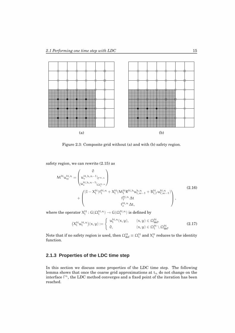
2.1 Performing one time step with LDC 15
(a) (b)
Figure 2.3: Composite grid without (a) and with (b) safety region.
safety region, we can rewrite (2.15) as
MHuH,nw =
0
uH,h,n−1∗
|ΓH,n
uH,h,n−1∗
|ΩH,nc
+
(I− XHl )fH,n
l + XHl (MH
l RH,huh,n
l,w−1 + BHl,Γu
H,nΓ,w−1)
fH,nΓ ∆t
fH,nc ∆t,
,
(2.16)
where the operator XHl : G(ΩH,n
l )→ G(ΩH,nl ) is defined by
(
XHl u
H,nl
)
(x, y) :=
uH,n
l (x, y), (x, y) ∈ ΩHdef,
0, (x, y) ∈ ΩHl \ΩH
def.(2.17)
Note that if no safety region is used, thenΩHdef ≡ ΩH
l and XHl reduces to the identity
function.
2.1.3 Properties of the LDC time step
In this section we discuss some properties of the LDC time step. The following
lemma shows that once the coarse grid approximations at tn do not change on the
interface Γn, the LDC method converges and a fixed point of the iteration has been
reached.
16 Chapter 2 - The LDC method for parabolic partial differential equations
Lemma 2.1
If uH,nΓ,w = uH,n
Γ,w−1 for a certain index w, then the LDC iteration converges and
uH,nq = uH,n
w , uh,nq = uh,n
w , (2.18)
for all q = w,w+ 1, . . .
Proof. Assume that uH,nΓ,w = uH,n
Γ,w−1 for a certain index w. From (2.11), we have that
uh,nw = uh,n
w−1, and hence, from (2.16),
MHuH,nw+1 =
0
uH,h,n−1∗
|ΓH,n
uH,h,n−1∗
|ΩH,nc
+
(I − XHl )fH,n
l + XHl (MH
l RH,huh,n
l,w + BHl,Γu
H,nΓ,w )
fH,nΓ ∆t
fH,nc ∆t,
=
0
uH,h,n−1∗
|ΓH,n
uH,h,n−1∗
|ΩH,nc
+
(I−XHl )fH,n
l +XHl (MH
l RH,huh,n
l,w−1+BHl,Γu
H,nΓ,w−1)
fH,nΓ ∆t
fH,nc ∆t,
=MHuH,n
w .
Because we have assumed MH to be invertible, we have uH,nw+1 = uH,n
w , for all grid
points in ΩH. Since ΓH,n ⊂ ΩH, we have uH,nΓ,w+1 = uH,n
Γ,w . By induction, we find
uH,nq = uH,n
w and uh,nq = uh,n
w , for all q = w,w + 1, . . .
Lemma 2.1 is the time-dependent equivalent of [1, Lemma 3.2]. Using a matrix
notation, equations (2.7) and (2.11) can be combined as follows
(
Mhl
)τ0 Wn
l,ΓPh,H 0
0 MHl BH
l,Γ 0
0 BHΓ,l MH
Γ BHΓ,c
0 0 BHc,Γ MH
c
uh,nl,w
uH,nl,w
uH,nΓ,w
uH,nc,w
=
0 0 0 0
XHl M
Hl R
H,h 0 XHl B
Hl,Γ 0
0 0 0 0
0 0 0 0
uh,nl,w−1
uH,nl,w−1
uH,nΓ,w−1
uH,nc,w−1
+
uH,h,n−1∗
|Ωh,nl
(I− XHl )uH,h,n−1
∗|ΩH,n
l
uH,h,n−1∗
|ΓH,n
uH,h,n−1∗
|ΩH,nc
+
Fh,nl ∆t
(I − XHl )fH,n
l
fH,nΓ δt
fH,nc δt
+
Znl,Γu
H,h,n−1∗
|Γh,n
0
0
0
. (2.19)
Equation (2.19) is an expression for the LDC iteration at time tn. It can also be
written using the short notation
MH,h uH,h,nw = SH,h uH,h,n
w−1 + uH,h,n−1∗
+ fH,h,n + zH,h,n−1. (2.20)
2.1 Performing one time step with LDC 17
The limit of the LDC iteration at time tn is indicated by
uH,h,n :=
uh,nl
uH,nl
uH,nΓ
uH,nc
. (2.21)
In (2.21) we removed the subscriptw that numbers the LDC iterations. Since uH,h,n
is the fixed point, one has
MH,h uH,h,n = SH,h uH,h,n + uH,h,n−1∗
+ fH,h,n + zH,h,n−1. (2.22)
With reference to the LDC method with no safety region, the following theorem
states that, if the LDC iteration converges, the fine and the coarse grid approxima-
tion coincide at the common points between fine and coarse grid.
Theorem 2.2
Consider an LDC time step and compute the defect term using no safety region.
Assume that the LDC iteration converges. Then the fixed point uH,h,n is such that
RH,huh,nl = uH
l . (2.23)
Proof. If no safety region is used, then XHl = I and equation (2.22) for the fixed
point can be written as
(
Mhl
)τ0 Wn
l,Γ 0
−MHl R
H,h MHl 0 0
0 BHΓ,l MH
Γ BHΓ,c
0 0 BHc,Γ MH
c
uh,nl
uH,nl
uH,nΓ
uH,nc
=
uH,h,n−1∗
|Ωh,nl
0
uH,h,n−1∗
|ΓH,n
uH,h,n−1∗
|ΩH,nc
+
Fh,nl ∆t
0,
fH,nΓ δt
fH,nc δt
+
Znl,Γu
H,h,n−1∗
|Γh,n
0
0
0
. (2.24)
The second equation of the system reads
MHl R
H,huh,nl +MH
l uH,nl = 0, (2.25)
which gives (2.23), since we supposed MH (and hence MHl ) to be invertible.
We finally write the system of equations that the limit of the LDC iteration satisfies
at time tn.
18 Chapter 2 - The LDC method for parabolic partial differential equations
Theorem 2.3
Consider an LDC time step and compute the defect term using no safety region.
Assume that the LDC iteration converges. Then uh,nl , uH,n
Γ and uH,nc satisfy the
following system of equations
(
Mhl
)τWn
l,Γ 0
BHΓ,lR
H,h MHΓ BH
Γ,c
0 BHc,Γ MH
c
uh,nl,w
uH,nΓ,w
uH,nc,w
=
uH,h,n−1∗
|Ωh,nl
uH,h,n−1∗
|ΓH,n
uH,h,n−1∗
|ΩH,nc
+
Fh,nl ∆t
fH,nΓ δt
fH,nc δt
+
Znl,Γ u
H,h,n−1∗
|ΓH,n
0
0
. (2.26)
Proof. Elimination of uH,nl from (2.24) gives (2.26).
Theorems 2.2 and 2.3 are the generalization to time-dependent problems of [1, The-
orem 3.3]. Note that (2.26) implies a discretization on the composite grid, while, for
solving that system, we have only used uniform grids and uniform grid solvers.
2.2 The LDC algorithm including regridding
In the previous section we explained how to perform the time step from tn−1 to tnusing LDC. For that we assumed to have a local grid Ωh,n
l suitable to cover the so-
lution’s high activity at tn. Moreover we assumed to know a solution uH,h,n−1∗
in all
the points of the composite grid ΩH,h,n = ΩH ∪ Ωh,nl at time tn−1. Using this infor-
mation, we could compute a composite grid solution at tn on ΩH,h,n := ΩH ∪Ωh,nl .
Including the boundary conditions for the global and the local problem into the so-
lution vector, we have an approximation of u at tn in all the points of ΩH,h,n.
Here we note that in a time-dependent problem it is likely that the solution’s high
activity moves and changes its size as time proceeds. As a consequence, the local
grid Ωh,nl used to perform the time step from tn−1 to tn might not be adequate to
cover the solution’s high activity also during the following time step. In general, we
expect thus to have Ωh,nl 6= Ωh,n+1
l , where Ωh,n+1l is the local grid used for com-
puting a solution at tn+1. We note that, in order to perform the time step from tnto tn+1, an approximation uH,h,n
∗must be available at tn in all the points of the
composite grid ΩH,h,n+1 = ΩH ∪ Ωh,n+1l . However, since the solution at tn was
computed on another composite grid, namely ΩH,h,n = ΩH ∪ Ωh,nl , a local approx-
imation of u at tn is directly available only in the common points between Ωh,nl
and Ωh,n+1l . On the remaining part of Ωh,n+1
l , i.e.
Ωh,n+1l := Ωh,n+1
l \ (Ωh,n+1l ∩ Ωh,n
l ), (2.27)
2.2 The LDC algorithm including regridding 19
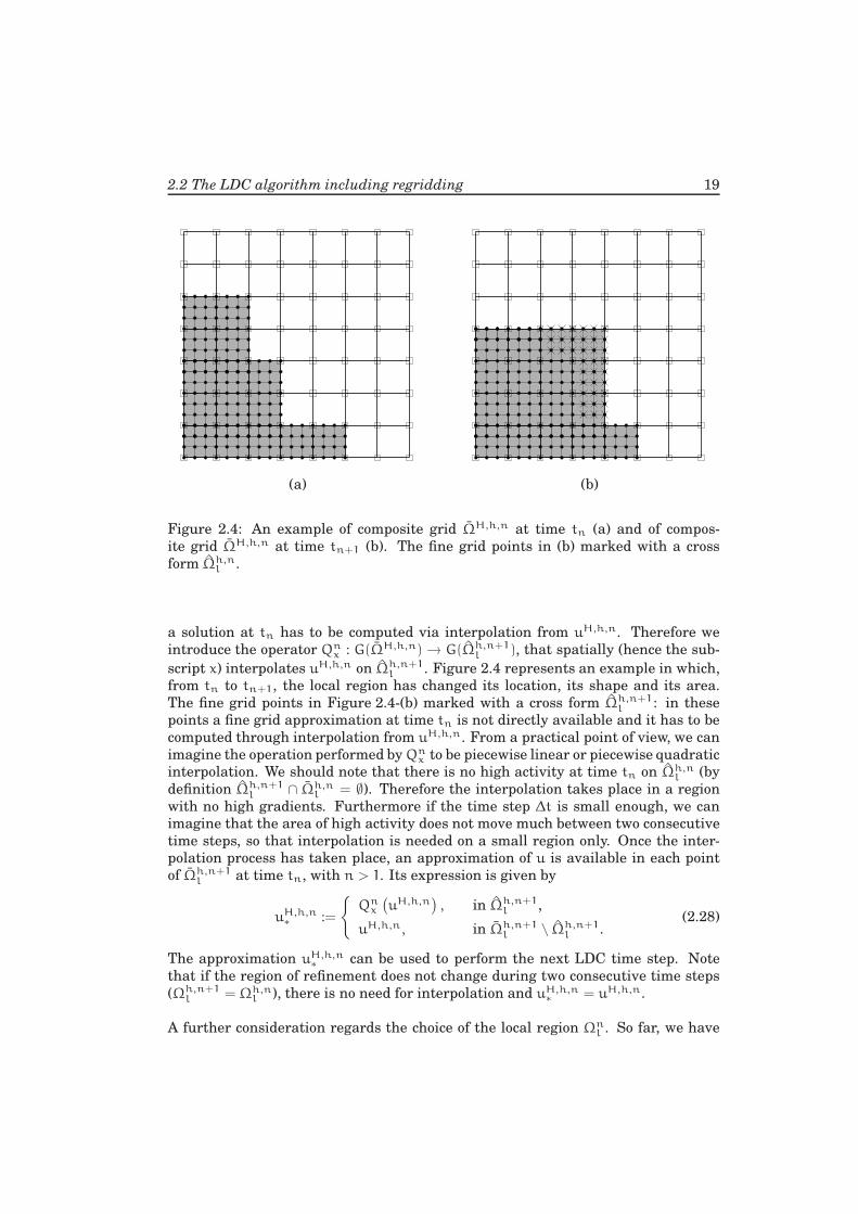
(a) (b)
Figure 2.4: An example of composite grid ΩH,h,n at time tn (a) and of compos-
ite grid ΩH,h,n at time tn+1 (b). The fine grid points in (b) marked with a cross
form Ωh,nl .
a solution at tn has to be computed via interpolation from uH,h,n. Therefore we
introduce the operator Qnx : G(ΩH,h,n) → G(Ωh,n+1
l ), that spatially (hence the sub-
script x) interpolates uH,h,n on Ωh,n+1l . Figure 2.4 represents an example in which,
from tn to tn+1, the local region has changed its location, its shape and its area.
The fine grid points in Figure 2.4-(b) marked with a cross form Ωh,n+1l : in these
points a fine grid approximation at time tn is not directly available and it has to be
computed through interpolation from uH,h,n. From a practical point of view, we can
imagine the operation performed byQnx to be piecewise linear or piecewise quadratic
interpolation. We should note that there is no high activity at time tn on Ωh,nl (by
definition Ωh,n+1l ∩ Ωh,n
l = ∅). Therefore the interpolation takes place in a region
with no high gradients. Furthermore if the time step ∆t is small enough, we can
imagine that the area of high activity does not move much between two consecutive
time steps, so that interpolation is needed on a small region only. Once the inter-
polation process has taken place, an approximation of u is available in each point
of Ωh,n+1l at time tn, with n > 1. Its expression is given by
uH,h,n∗
:=
Qn
x
(
uH,h,n)
, in Ωh,n+1l ,
uH,h,n, in Ωh,n+1l \ Ωh,n+1
l .(2.28)
The approximation uH,h,n∗
can be used to perform the next LDC time step. Note
that if the region of refinement does not change during two consecutive time steps
(Ωh,n+1l = Ωh,n
l ), there is no need for interpolation and uH,h,n∗
= uH,h,n.
A further consideration regards the choice of the local region Ωnl . So far, we have
20 Chapter 2 - The LDC method for parabolic partial differential equations
assumed it to be given, but in practice its position is not a priori known. At every
time tn it has to be determined on the basis of the solution’s features at that time
level. Many techniques have been proposed in the literature of adaptive methods to
detect where refinement is needed. In principle one can use any kind of criterion
which is suitable for one’s specific application. Throughout this thesis we will use
the method proposed in [10, 11, 65]. In [10, 11, 65] a positive weight function wij is
introduced to determine which coarse grid boxes Bij := (xi, xi+1)× (yj, yj+1) require
refinement. The weight function wij is meant to be an indicator of the solution’s
roughness. The values wij are computed on each box Bij from the gradient of the
first coarse grid approximation uH,n0 . After that a smoothing filter, an averaging
and a normalization procedure are applied. At the end the mean value of the weight
function is 1 and the boxes Bij for which wij > ǫ are labelled for refinement. The
threshold value ǫ is a user-specified parameter. Greater numerical values of ǫ result
in a tighter local region, while smaller values of ǫ make the area of Ωnl larger.
A suitable value for ǫ should therefore be determined on the basis of the specific
problem that has to be solved. Typical values for ǫ range from 1.5 to 3. Further
details on this method can be found in [10, 11, 65].
In Section 2.1 we considered the LDC time step and here we discussed a regridding
strategy. We are now ready to formulate the LDC algorithm for solving parabolic
partial-differential equations.
Algorithm 2.4 (LDC algorithm for parabolic problems)
FOR LOOP, n = 1, 2, . . . , tend/∆t
INITIALIZATION
• Provide initial values uH,h,n−1∗
on the coarse grid ΩH. If
n = 1, set uH,h,n−1∗
|ΩH from the initial condition. Other-
wise, set
uH,h,n−1∗
|ΩH = uH,h,n−1|ΩH .
• Compute a global coarse grid approximation uH,n0 solving
problem (2.3).
• Choose a region of refinement Ωnl , introduce a fine grid
Ωh,nl on it and a time step δt = ∆t/τ.
• Provide initial values ϕH,h,n−1∗
on the remaining points ofΩH,h,n = ΩH,n ∪ Ωh,n
l . If n = 1, use the initial condition. If
n > 1 and ΩH,h,nl ≡ ΩH,h,n−1
l , set
uH,h,n−1∗
|ΩH,h,nl
= uH,h,n−1|ΩH,h,n−1l
.
If n > 1 and ΩH,h,nl 6= ΩH,h,n−1
l , set
uH,h,n−1∗
=
Qn
x (uH,h,n−1), on Ωh,nl ,
uH,h,n−1, on ΩH,h,nl \ Ωh,n
l .
2.2 The LDC algorithm including regridding 21
• Use uH,n0 to provide a boundary condition for the local prob-
lem.
• Compute a local approximation uh,nl,0 solving the local prob-
lem (2.11).
ITERATION, w = 1, 2, . . .
• Use uh,nl,w−1 to compute an estimate dH,n
l,w−1 of the coarse grid
local discretization error as in (2.13).
• Compute a more accurate global approximation uH,nw solv-
ing a modified global problem as in (2.16).
• Use uH,nw to update the boundary condition for the local
problem.
• Compute a local solution uh,nl,w with updated boundary con-
ditions.
END ITERATION ON w
• The solution on the composite grid at time tn is uH,h,n (re-
move the subscript that numbers the LDC iterations).
END FOR LOOP ON n
Algorithm 2.4 shows that initial values uH,h,n−1∗
are provided in two stages. In order
to compute the first coarse grid approximation uH,n0 , it is sufficient to know uH,h,n−1
∗
on ΩH; for this purpose, the coarse grid restriction of the composite grid solution at
the previous time step can be used. Once uH,n0 is computed and the new region
of refinement Ωnl is chosen, initial values uH,h,n−1
∗are provided also at the points
of ΩH,h,n that lie in the region of refinement. In this case, space interpolation is
necessary whenever the new local region does not coincide with the local region
used during the previous time step. After solving the fine grid problem too, an iter-
ative procedure is triggered, and a global and a local solution at the new time level
iteratively improve each other. A suitable stopping criterion for the LDC iteration
is provided by Lemma 2.1. Note that each LDC iteration consists in the entire re-
computation of the time step ∆t. For a good performance in solving the transient
problem, it is thus desirable that only a small number of LDC iterations are needed
at each time step. However, as it happens in stationary cases, it turns that LDC
converges very fast. The convergence behavior of the LDC algorithm for parabolic
problems is the topic of Chapter 3 of this thesis.
When presenting the LDC method for time-dependent problems we have used the
implicit Euler scheme for time discretization. We should notice here that this is
not restrictive and that other implicit methods for time discretization (e.g. Runge-
Kutta schemes) might be applied as well. Moreover we are not constrained to use
the same scheme for the global and for the local grid. While it is possible to use
an explicit method on the fine grid, it is crucial for the effectiveness of LDC that
an implicit time integrator is adopted globally. In fact, if we would use an explicit
22 Chapter 2 - The LDC method for parabolic partial differential equations
time integration scheme on the global grid, the matrix MH would be diagonal and
the matrices BHl,Γ , BH
Γ,l, BHΓ,c, BH
c,Γ would be all zero, see (2.7). As a consequence the
effect of the defect correction on ΩH,nl would be the replacement of the coarse grid
solution with the fine grid approximation. Moreover the coarse grid solution would
not change on the coarse grid points outside the area of refinement. Clearly in such
a case LDC coincides with LUGR.
One of the most interesting features of the LDC algorithm we are proposing is
the possibility of performing the time integration on the local region with a time
step δt < ∆t. This is a feature, not a requirement of the method; it is very well pos-
sible to choose the same time step on both the global and the local grid. In general
we expect however that a solution characterized by relatively high spatial gradients
in a certain region of the domain has, in that same region, relatively high values of
the time derivative too; an intuitive example is given by a front propagation. For
this reason the use of a time step ∆t on the local grid might be not adequate to
represent the fast phenomena occurring there. Moreover, if we would perform time
integration locally with the same step as on the global grid, the discretization er-
ror on the fine grid might be heavily dominated by the temporal component, which
would make the effect of solving the local problem with a grid size h < H useless.
We note that it is common that adaptive grid methods for time-dependent problems
provide the possibility of using smaller time steps locally, see for instance LUGR
or [25, 57]. In the case of LDC this has a further implication: the defect correction,
which is used to compute a more accurate global approximation at tn, improves the
coarse grid solution not only in its spatial component of the error, but also in the
temporal part. In practice the parameters H, ∆t, h and δt are to be chosen on the
basis of the physical problem that has to be solved and on the discretization schemes
adopted globally and locally.
2.3 Numerical experiments
In this section we present two numerical examples. The first one, Section 2.3.1, is
a 2D numerical experiment in which the LDC technique is compared with a stan-
dard uniform grid solver. We show that LDC can achieve the same accuracy as
the uniform grid solver, while requiring the computation of a smaller number of
unknowns and being thus a more efficient method. In the second example, Sec-
tion 2.3.2, we compare LDC and LUGR. We show that LUGR may already fail to
produce reliable results for a simple 1D problem, whereas LDC leads to an accu-
rate solution. This example illustrates the superior robustness of the LDC method
over LUGR.

2.3 Numerical experiments 23
2.3.1 Example 1: a 2D convection-diffusion problem
In this section we present the results of a 2D numerical experiment. We choose
Ω = (0, 1)2 and Θ = (0, 2], and we solve the following problem
∂u
∂t+ v · ∇u = λ∇2u, in Ω×Θ,
u = 0, on ∂Ω×Θ,
u = exp(
−100(
(x− 0.3)2
+ (y− 0.3)2))
, in Ω, t = 0,
(2.29)
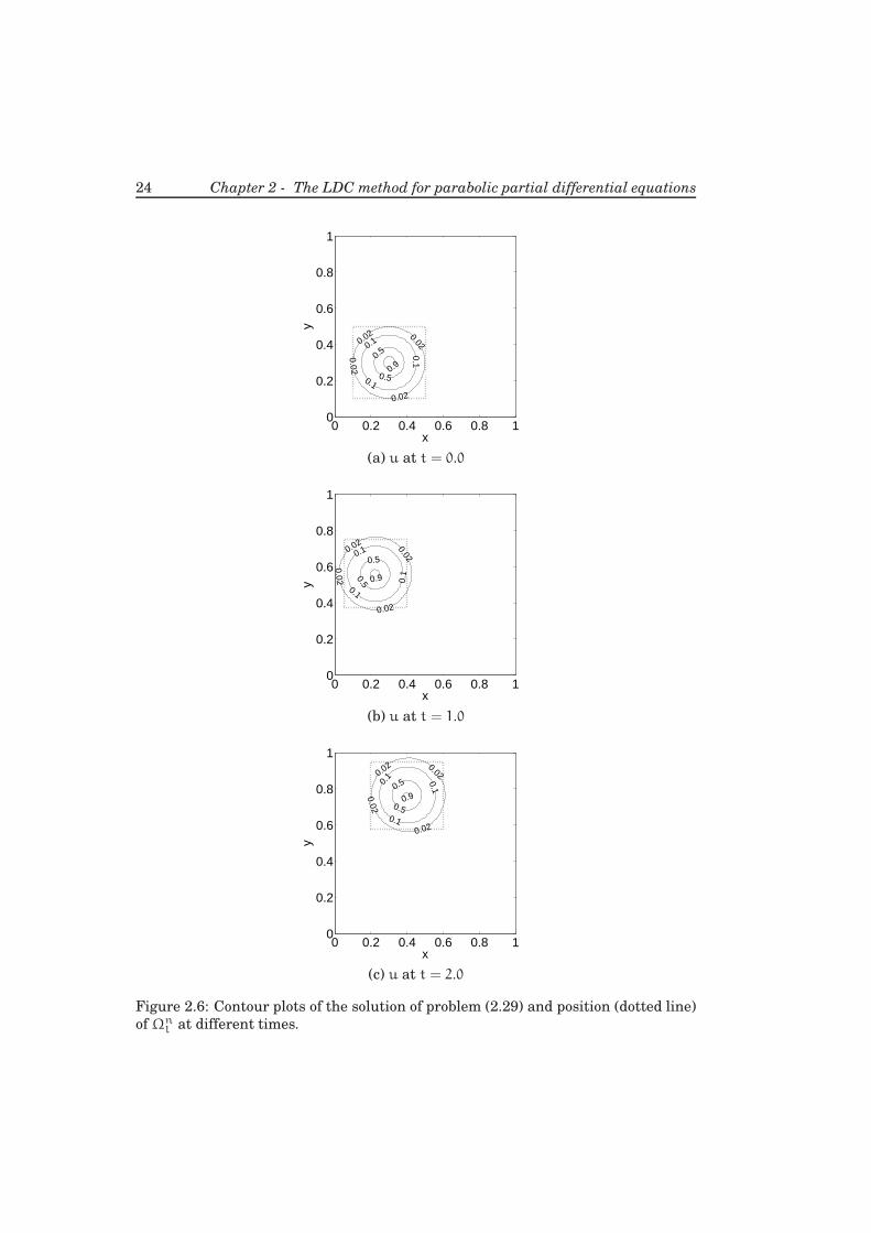
where v = v(x, y) = (y − 0.5,−x + 0.5), see Figure 2.5. Note that L ≡ λ∇2 − v · ∇in (2.29); we choose λ = 10−4 > 0 so that L is an elliptic operator. Figure 2.6 shows
the contour plots of u for different values of time. The solution of problem (2.29) has
at each time a region of high activity that covers a limited part ofΩ. Figure 2.6 also
shows (dotted line) the location of the local regionΩnl in one of our LDC runs.
Problem (2.29) is solved using LDC with different values of H, ∆t, h and δt (see
Table 2.1). In all the LDC runs, one and only one LDC iteration is performed at
each time step ∆t; to recall this, in Table 2.1 we write LDC1, where the subscript
indicates the number of LDC iterations at each time step. In all our runs the spatial
discretization is performed using finite differences; in particular the second order
centered differences scheme is applied both on the global and on the local grid.
The time discretization is performed using the first order implicit Euler scheme
both globally and locally. The position and the size of the local region are deter-
mined at each time step using the already mentioned algorithm which is described
in [10, 11, 65]; we choose a threshold value ǫ = 3. For simplicity of implementation
in all our runs the local regionΩnl has always a rectangular shape. Furthermore we
use no safety region when computing the defect. The operator Qnx performs piece-
wise linear interpolation from the coarse grid values. Also Ph,H performs piecewise
0 0.2 0.4 0.6 0.8 10
0.2
0.4
0.6
0.8
1
x
y
Figure 2.5: Plot of the velocity field v = (y− 0.5,−x+ 0.5).
24 Chapter 2 - The LDC method for parabolic partial differential equations
0.02 0.02
0.02
0.02
0.1
0.1
0.1
0.5
0.50.9
x
y
0 0.2 0.4 0.6 0.8 10
0.2
0.4
0.6
0.8
1
(a) u at t = 0.0
0.02 0.02
0.02
0.02
0.1
0.1
0.1
0.5
0.5 0.9
x
y
0 0.2 0.4 0.6 0.8 10
0.2
0.4
0.6
0.8
1
(b) u at t = 1.0
0.02 0.02
0.02
0.02
0.1 0.1
0.1
0.5
0.50.9
x
y
0 0.2 0.4 0.6 0.8 10
0.2
0.4
0.6
0.8
1
(c) u at t = 2.0
Figure 2.6: Contour plots of the solution of problem (2.29) and position (dotted line)
of Ωnl at different times.
2.3 Numerical experiments 25
Grid and time step ǫ∞ Total number of unknowns
H ∆t σ = τ LDC1 Unif.LDC1
(coarse + fine)Unif. Unif.
LDC1
3 3.6·10−1 3.7·10−1 7.2·103 + 3.1·104 1.0·105 2.7
H0 ∆t0 5 2.8·10−1 2.8·10−1 7.2·103 + 1.4·105 4.9·105 3.3
7 2.3·10−1 2.3·10−1 7.2·103 + 4.0·105 1.7·106 3.3
H0
2∆t04
3 1.7·10−1 1.7·10−1 1.2·105 + 4.4·105 1.7·106 3.0
5 1.1·10−1 1.1·10−1 1.2·105 + 2.0·106 7.9·106 3.7
7 8.6·10−2 8.6·10−2 1.2·105 + 5.6·106 2.2·107 3.8
H0
4∆t016
3 5.4·10−2 5.4·10−2 2.0·106 + 6.8·106 2.7·107 3.1
5 3.3·10−2 3.3·10−2 2.0·106 + 3.2·107 1.3·108 3.8
7 2.4·10−2 2.4·10−2 2.0·106 + 8.7·107 3.5·108 3.9
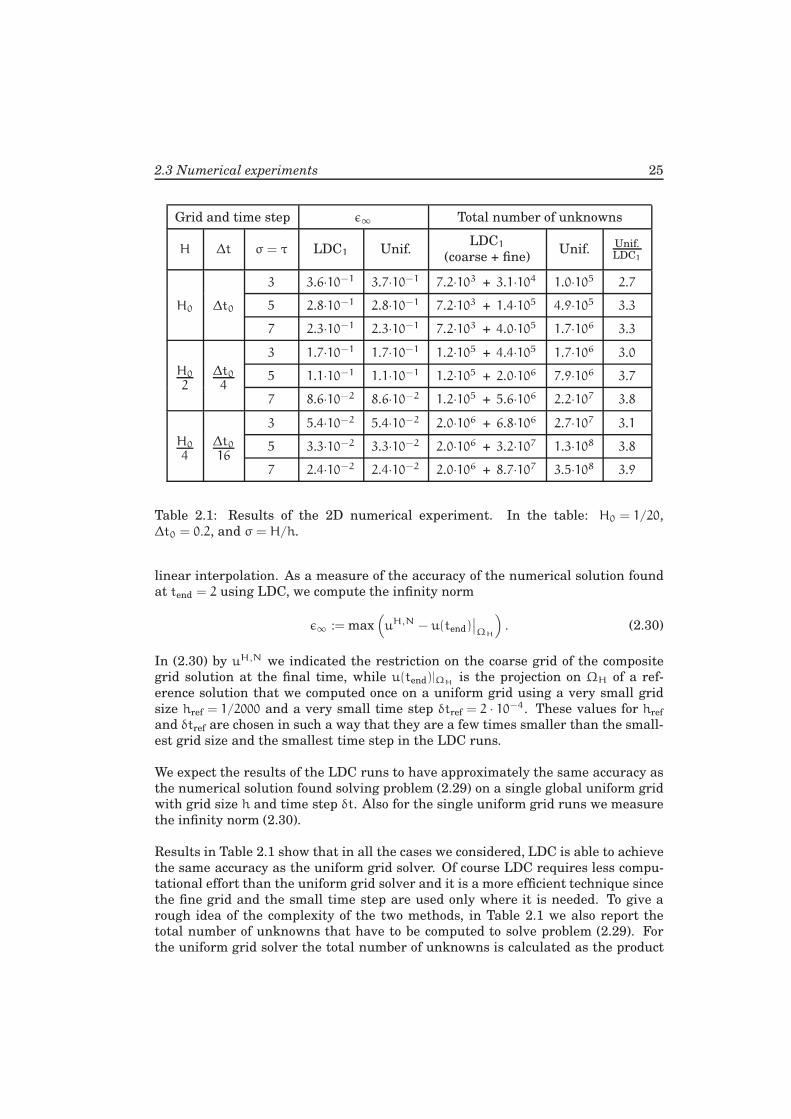
Table 2.1: Results of the 2D numerical experiment. In the table: H0 = 1/20,
∆t0 = 0.2, and σ = H/h.
linear interpolation. As a measure of the accuracy of the numerical solution found
at tend = 2 using LDC, we compute the infinity norm
ǫ∞ := max(
uH,N − u(tend)∣
∣
ΩH
)
. (2.30)
In (2.30) by uH,N we indicated the restriction on the coarse grid of the composite
grid solution at the final time, while u(tend)|ΩHis the projection on ΩH of a ref-
erence solution that we computed once on a uniform grid using a very small grid
size href = 1/2000 and a very small time step δtref = 2 · 10−4. These values for href
and δtref are chosen in such a way that they are a few times smaller than the small-
est grid size and the smallest time step in the LDC runs.
We expect the results of the LDC runs to have approximately the same accuracy as
the numerical solution found solving problem (2.29) on a single global uniform grid
with grid size h and time step δt. Also for the single uniform grid runs we measure
the infinity norm (2.30).
Results in Table 2.1 show that in all the cases we considered, LDC is able to achieve
the same accuracy as the uniform grid solver. Of course LDC requires less compu-
tational effort than the uniform grid solver and it is a more efficient technique since
the fine grid and the small time step are used only where it is needed. To give a
rough idea of the complexity of the two methods, in Table 2.1 we also report the
total number of unknowns that have to be computed to solve problem (2.29). For
the uniform grid solver the total number of unknowns is calculated as the product
26 Chapter 2 - The LDC method for parabolic partial differential equations
of the number of grid points and the number of time steps. For LDC this product
is given separately for the coarse grid and for the sum of all the local problems; the
numbers in Table 2.1 already take into account that in LDC1 each time step ∆t has
to be repeated twice (computation of a first approximation at tn plus one defect cor-
rection). From the table we can see that in our example, when we use LDC, we have
to compute a total number of unknowns which is about three times less than when
the uniform grid solver is adopted. The gain increases when higher factors of grid
and time refinement are used or when the high activity is more localized than in the
example presented here. The LDC algorithm can be generalized for 3D problems in
a straightforward manner. The gain of LDC in 3D is even higher than in 2D because
the number of unknowns is proportional to the volume rather than the area of the
high activity zone.
To conclude, this example shows that LDC can achieve the same accuracy as a uni-
form grid solver that uses the same grid size and time step as in the LDC local
problem. Yet, LDC is a more efficient method than the uniform grid solver: in LDC
the fine grid is adaptively placed only where it needs to be and this guarantees
a saving in the total number of unknowns that have to be computed to solve the
problem.
2.3.2 Example 2: comparison between LDC and LUGR
In this section we present the results of a 1D numerical experiment aimed at show-
ing the robustness of the LDC method. We choose Ω = (0, 2) and Θ = (0, 1], and we
solve the partial differential equation
∂u
∂t+ v
∂u
∂x−∂2u
∂x2= f, in Ω×Θ, (2.31)
with v = 1. We notice that in (2.31)
L ≡ −v∂
∂x+∂2
∂x2. (2.32)
Clearly L is thus a convection–diffusion operator. The initial condition, the Dirichlet
boundary conditions and the source term f are chosen in such a way that the exact
analytical solution of the problem is
u(x, t) =(
tanh(
100(x − 1/8− t))
+ 1)
(
1− e−2t)
. (2.33)
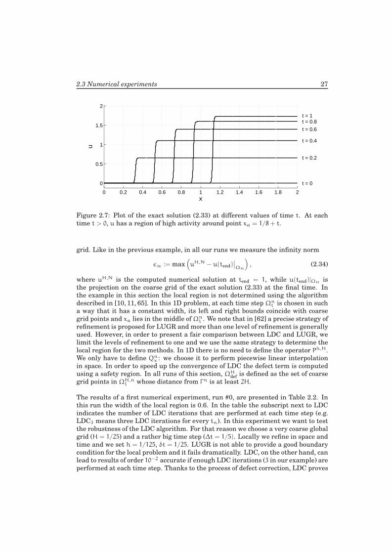
At time t > 0 the exact solution (2.33) has a region of high activity around point
xa = 1/8+ t (see Figure 2.7).
The problem above is solved using both LDC and LUGR. Equation (2.31) is dis-
cretized in space using finite differences; in particular, both globally and locally a
second order centered differences scheme is adopted. The time discretization is per-
formed with the first order implicit Euler scheme both on the global and on the local
2.3 Numerical experiments 27
0 0.2 0.4 0.6 0.8 1 1.2 1.4 1.6 1.8 2
0
0.5
1
1.5
2
t = 0
t = 0.2
t = 0.4
t = 0.6
t = 0.8t = 1
x
u
Figure 2.7: Plot of the exact solution (2.33) at different values of time t. At each
time t > 0, u has a region of high activity around point xa = 1/8+ t.
grid. Like in the previous example, in all our runs we measure the infinity norm
ǫ∞ := max(
uH,N − u(tend)∣
∣
ΩH
)
, (2.34)
where uH,N is the computed numerical solution at tend = 1, while u(tend)|ΩHis
the projection on the coarse grid of the exact solution (2.33) at the final time. In
the example in this section the local region is not determined using the algorithm
described in [10, 11, 65]. In this 1D problem, at each time step Ωnl is chosen in such
a way that it has a constant width, its left and right bounds coincide with coarse
grid points and xa lies in the middle ofΩnl . We note that in [62] a precise strategy of
refinement is proposed for LUGR and more than one level of refinement is generally
used. However, in order to present a fair comparison between LDC and LUGR, we
limit the levels of refinement to one and we use the same strategy to determine the
local region for the two methods. In 1D there is no need to define the operator Ph,H.
We only have to define Qnx : we choose it to perform piecewise linear interpolation
in space. In order to speed up the convergence of LDC the defect term is computed
using a safety region. In all runs of this section, ΩHdef is defined as the set of coarse
grid points in ΩH,nl whose distance from Γn is at least 2H.
The results of a first numerical experiment, run #0, are presented in Table 2.2. In
this run the width of the local region is 0.6. In the table the subscript next to LDC
indicates the number of LDC iterations that are performed at each time step (e.g.
LDC3 means three LDC iterations for every tn). In this experiment we want to test
the robustness of the LDC algorithm. For that reason we choose a very coarse global
grid (H = 1/25) and a rather big time step (∆t = 1/5). Locally we refine in space and
time and we set h = 1/125, δt = 1/25. LUGR is not able to provide a good boundary
condition for the local problem and it fails dramatically. LDC, on the other hand, can
lead to results of order 10−2 accurate if enough LDC iterations (3 in our example) are
performed at each time step. Thanks to the process of defect correction, LDC proves
28 Chapter 2 - The LDC method for parabolic partial differential equations
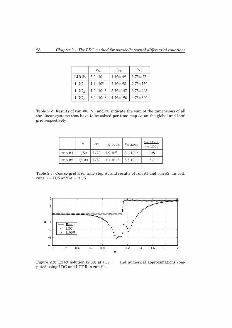
ǫ∞ Ng Nl
LUGR 5.2 · 101 1·49= 49 1·75= 75LDC1 1.9 · 100 2·49= 98 2·75=150LDC2 1.0 · 10−1 3·49=147 3·75=225LDC3 3.4 · 10−2 4·49=196 4·75=300
Table 2.2: Results of run #0. Ng and Nl indicate the sum of the dimensions of all
the linear systems that have to be solved per time step ∆t on the global and local
grid respectively.
H ∆t ǫ∞ ,LUGR ǫ∞ ,LDC1
ǫ∞ ,LUGR
ǫ∞ ,LDC1
run #1 1/50 1/20 3.9·100 3.6·10−2 108
run #2 1/100 1/80 3.1·10−2 5.5·10−3 5.6
Table 2.3: Coarse grid size, time step ∆t and results of run #1 and run #2. In both
runs h = H/5 and δt = ∆t/5.
0 0.2 0.4 0.6 0.8 1 1.2 1.4 1.6 1.8 2−4
−3
−2
−1
0
1
2
x
u
ExactLDCLUGR
Figure 2.8: Exact solution (2.33) at tend = 1 and numerical approximations com-
puted using LDC and LUGR in run #1.
2.3 Numerical experiments 29
to be a more robust technique than LUGR. Table 2.2 also shows that increasing the
number of LDC iterations, we proportionally increase the number of unknowns that
have to be computed per time step ∆t: each defect correction (see Algorithm 2.4)
means in fact reperforming the entire time step ∆t again and computing new (more
accurate) coarse and fine grid approximations. In particular, we have that
NLDC1
NLUGR
= 2, (2.35)
where N is the total number of unknowns (global grid + local grid) per time step.
With total number of unknowns we mean the sum of the dimensions of all the linear
systems that have to be solved per time step.
In Table 2.3 we present the results of other two numerical simulations: run #1 and
run #2. In both of them the width of the local region is 0.2, the factors of grid and
time refinement are both equal to 5 and we only consider the comparison between
LUGR and LDC1. In run #1 we have a situation similar to run #0: LUGR fails,
while the approximation computed using LDC has an accuracy of order 10−2 (see
Figure 2.8). Keeping in mind that we are using a second order method in space and
a first order method in time, in run #2 we take H twice as small and ∆t four times
as small with respect to run #1. LUGR finally gives meaningful results; yet LDC is
a factor 5.6 more accurate than LUGR, costing only twice as much in terms of total
number of unknowns per time step, see (2.35).

Chapter 3
Convergence properties of LDC
In Chapter 2 we introduced the LDC algorithm for parabolic problems and we ex-
plained that the method is similar to the LUGR technique studied in [62]. More-
over, we showed by means of numerical experiments that LDC is more robust than
LUGR: this is because in LDC the local solution improves the solution globally
through a defect correction. The robustness of LDC comes at a cost though, because
the defect corrections involve more computational work. For LDC to be competitive
with other techniques, it is thus desirable that only a small number of iterations are
necessary at every time step. This chapter is therefore focused on the convergence
properties of the LDC method for parabolic problems. In particular, we are inter-
ested in investigating the dependency of the LDC convergence rate on the time step
for the coarse grid problem.
The convergence properties of LDC have been previously studied for stationary
problems. In [4] a two-dimensional Poisson’s equation is considered: if the defect
is computed using a safety region, it is proved that iteration errors reduce propor-
tionally to H2, where H is the coarse grid size. If no safety region is adopted, results
of numerical experiments show that iteration errors reduce linearly with H. In [53]
a convergence analysis is carried out for a case where the local domain has an an-
nular shape. In general, even for rather complicated applications, it is observed by
many authors (see [1, 2, 29, 33, 47]) that LDC has very good convergence properties
and that one or two iterations are usually sufficient for convergence. The conditions
for one-step convergence of LDC for elliptic problems are given in [5].
The analysis and the one-dimensional numerical experiments of this chapter have
previously been presented in [46].
32 Chapter 3 - Convergence properties of LDC
3.1 The iteration matrix
In this section we want to find an expression for the matrix that describes the LDC
iteration at time tn. We slightly simplify the notation introduced in Chapter 2. In
the previous chapter, the local domain at time tn was denoted by Ωnl , where the
superscript n was introduced to take into account that the local region might be
different at different time levels. Throughout this chapter we will only consider the
LDC iteration at one specific time step; at this specific time step we will always
suppose the local region to be given. The superscript n is thus not needed in this
context and we will omit it: the local domain will simply be denoted by Ωl. The
same is done for other symbols: in this chapter the interface between coarse and
fine grid at time tn will be denoted just by Γ (not Γn), the coarse grid points on the
interface by ΓH, the coarse grid points in the area of refinement by ΩHl , etc.
In order to find an expression for the matrix that describes the LDC iteration at
time tn, we follow a similar approach as done in [4] for stationary problems. In [4]
the LDC iteration is expressed in terms of the iteration that takes place on ΓH only
and it is shown that, if the iteration on ΓH converges, then the entire LDC iteration
converges. Previously, other approaches were proposed. In [34] the LDC iteration
for elliptic problems is expressed in terms of grid functions that operate on Γh, i.e.
the set of fine grid points on the interface. In [28], with reference to boundary value
problems, the LDC iteration that takes place on the whole set of composite grid
points is considered.
With uH,h,n defined as in (2.21), we introduce the iteration error of the LDC method
by
eH,h,nw := uH,h,n
w − uH,h,n. (3.1)
If we subtract (2.20) and (2.22), we can write the expression for successive iteration
errors
MH,heH,h,nw = SH,heH,h,n
w−1 . (3.2)
Note that the convergence of the LDC method does not depend on the source term,
on the Dirichlet boundary conditions and on the solution at the previous time step.
Definitions of MH,h and SH,h enables us to rewrite (3.2) as
(
Mhl
)τ0 Wn
l,Γ 0
0 MHl BH
l,Γ 0
0 BHΓ,l MH
Γ BHΓ,c
0 0 BHc,Γ MH
c
eh,nl,w
eH,nl,w
eH,nΓ,w
eH,nc,w
=
0
XHl M
Hl R
H,heh,nl,w−1 + XH
l BHl,Γe
H,nΓ,w−1
0
0
. (3.3)
The first equation of this system yields
eh,nl,w = −
(
(Mhl )τ)−1
Wnl,Γe
H,nΓ,w . (3.4)
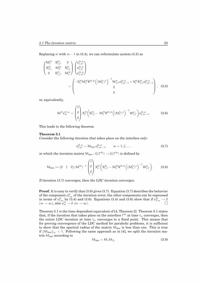
3.1 The iteration matrix 33
Replacing w with w− 1 in (3.4), we can reformulate system (3.3) as
MHl BH
l,Γ 0
BHΓ,l MH
Γ BHΓ,c
0 BHc,Γ MH
c
eH,nl,w
eH,nΓ,w
eH,nc,w
=
−XHl M
Hl R
H,h(
(Mhl )τ)−1
Wnl,Γe
H,nΓ,w−1 + XH
l BHl,Γe
H,nΓ,w−1
0
0
, (3.5)
or, equivalently,
MHeH,nw =
I
0
0
XHl
(
BHl,Γ −MH
l RH,h(
(Mhl )τ)−1
Wnl,Γ
)
eH,nΓ,w−1. (3.6)
This leads to the following theorem.
Theorem 3.1
Consider the following iteration that takes place on the interface only:
eH,nΓ,w = Miter e
H,nΓ,w−1, w = 1, 2, . . . (3.7)
in which the iteration matrix Miter : G(ΓH)→ G(ΓH) is defined by
Miter :=(
0 I 0)
(MH)−1
I
0
0
XHl
(
BHl,Γ −MH
l RH,h(
(Mhl )τ)−1
Wnl,Γ
)
. (3.8)
If iteration (3.7) converges, then the LDC iteration converges.
Proof. It is easy to verify that (3.6) gives (3.7). Equation (3.7) describes the behavior
of the component eHΓ,w of the iteration error; the other components can be expressed
in terms of eHΓ,w by (3.4) and (3.6). Equations (3.4) and (3.6) show that if eH
Γ,w → 0
(w→∞), also eHw → 0 (w→∞).
Theorem 3.1 is the time-dependent equivalent of [4, Theorem 2]. Theorem 3.1 states
that, if the iteration that takes place on the interface ΓH at time tn converges, then
the entire LDC iteration at time tn converges to a fixed point. This means that
for proving convergence of the LDC method for parabolic problems, it is sufficient
to show that the spectral radius of the matrix Miter is less than one. This is true
if ‖Miter‖∞ < 1. Following the same approach as in [4], we split the iteration ma-
trix Miter according to
Miter = M1M2, (3.9)
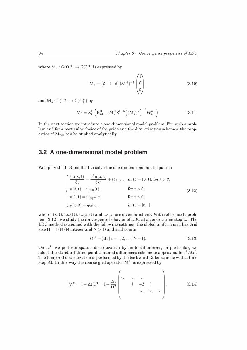
34 Chapter 3 - Convergence properties of LDC
where M1 : G(ΩHl )→ G(ΓH) is expressed by
M1 =(
0 I 0)
(MH)−1
I
0
0
, (3.10)
and M2 : G(ΓH)→ G(ΩHl ) by
M2 = XHl
(
BHl,Γ −MH
l RH,h(
(Mhl )τ)−1
Wnl,Γ
)
. (3.11)
In the next section we introduce a one-dimensional model problem. For such a prob-
lem and for a particular choice of the grids and the discretization schemes, the prop-
erties of Miter can be studied analytically.
3.2 A one-dimensional model problem
We apply the LDC method to solve the one-dimensional heat equation
∂u(x, t)
∂t=∂2u(x, t)
∂x2+ f(x, t), in Ω = (0, 1), for t > 0,
u(0, t) = ψleft(t), for t > 0,
u(1, t) = ψright(t), for t > 0,
u(x, 0) = ϕ0(x), in Ω = [0, 1],
(3.12)
where f(x, t), ψleft(t), ψright(t) and ϕ0(x) are given functions. With reference to prob-
lem (3.12), we study the convergence behavior of LDC at a generic time step tn. The
LDC method is applied with the following settings: the global uniform grid has grid
size H = 1/N (N integer and N > 1) and grid points
ΩH = iH | i = 1, 2, . . . , N− 1. (3.13)
On ΩH we perform spatial discretization by finite differences; in particular, we
adopt the standard three-point centered differences scheme to approximate ∂2/∂x2.
The temporal discretization is performed by the backward Euler scheme with a time
step ∆t. In this way the coarse grid operatorMH is expressed by
MH = I− ∆t LH = I−∆t
H2
. . .. . .
. . .
1 −2 1
. . .. . .
. . .
. (3.14)
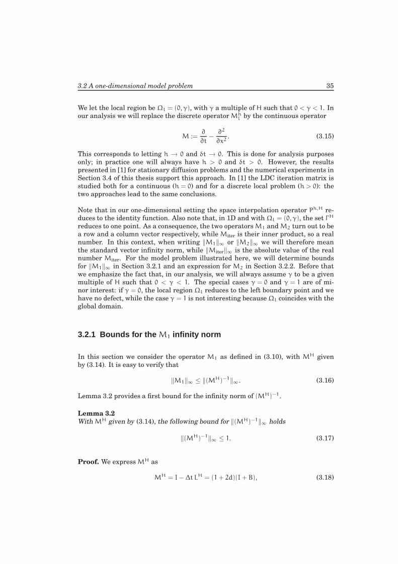
3.2 A one-dimensional model problem 35
We let the local region be Ωl = (0, γ), with γ a multiple of H such that 0 < γ < 1. In
our analysis we will replace the discrete operatorMhl by the continuous operator
M :=∂
∂t−∂2
∂x2. (3.15)
This corresponds to letting h → 0 and δt → 0. This is done for analysis purposes
only; in practice one will always have h > 0 and δt > 0. However, the results
presented in [1] for stationary diffusion problems and the numerical experiments in
Section 3.4 of this thesis support this approach. In [1] the LDC iteration matrix is
studied both for a continuous (h = 0) and for a discrete local problem (h > 0): the
two approaches lead to the same conclusions.
Note that in our one-dimensional setting the space interpolation operator Ph,H re-
duces to the identity function. Also note that, in 1D and with Ωl = (0, γ), the set ΓH
reduces to one point. As a consequence, the two operatorsM1 andM2 turn out to be
a row and a column vector respectively, while Miter is their inner product, so a real
number. In this context, when writing ‖M1‖∞ or ‖M2‖∞ we will therefore mean
the standard vector infinity norm, while ‖Miter‖∞ is the absolute value of the real
number Miter. For the model problem illustrated here, we will determine bounds
for ‖M1‖∞ in Section 3.2.1 and an expression for M2 in Section 3.2.2. Before that
we emphasize the fact that, in our analysis, we will always assume γ to be a given
multiple of H such that 0 < γ < 1. The special cases γ = 0 and γ = 1 are of mi-
nor interest: if γ = 0, the local region Ωl reduces to the left boundary point and we
have no defect, while the case γ = 1 is not interesting because Ωl coincides with the
global domain.
3.2.1 Bounds for the M1 infinity norm
In this section we consider the operator M1 as defined in (3.10), with MH given
by (3.14). It is easy to verify that
‖M1‖∞ ≤ ‖(MH)−1‖∞ . (3.16)
Lemma 3.2 provides a first bound for the infinity norm of (MH)−1.
Lemma 3.2
With MH given by (3.14), the following bound for ‖(MH)−1‖∞ holds
‖(MH)−1‖∞ ≤ 1. (3.17)
Proof. We express MH as
MH = I− ∆t LH = (1+ 2d)(I + B), (3.18)
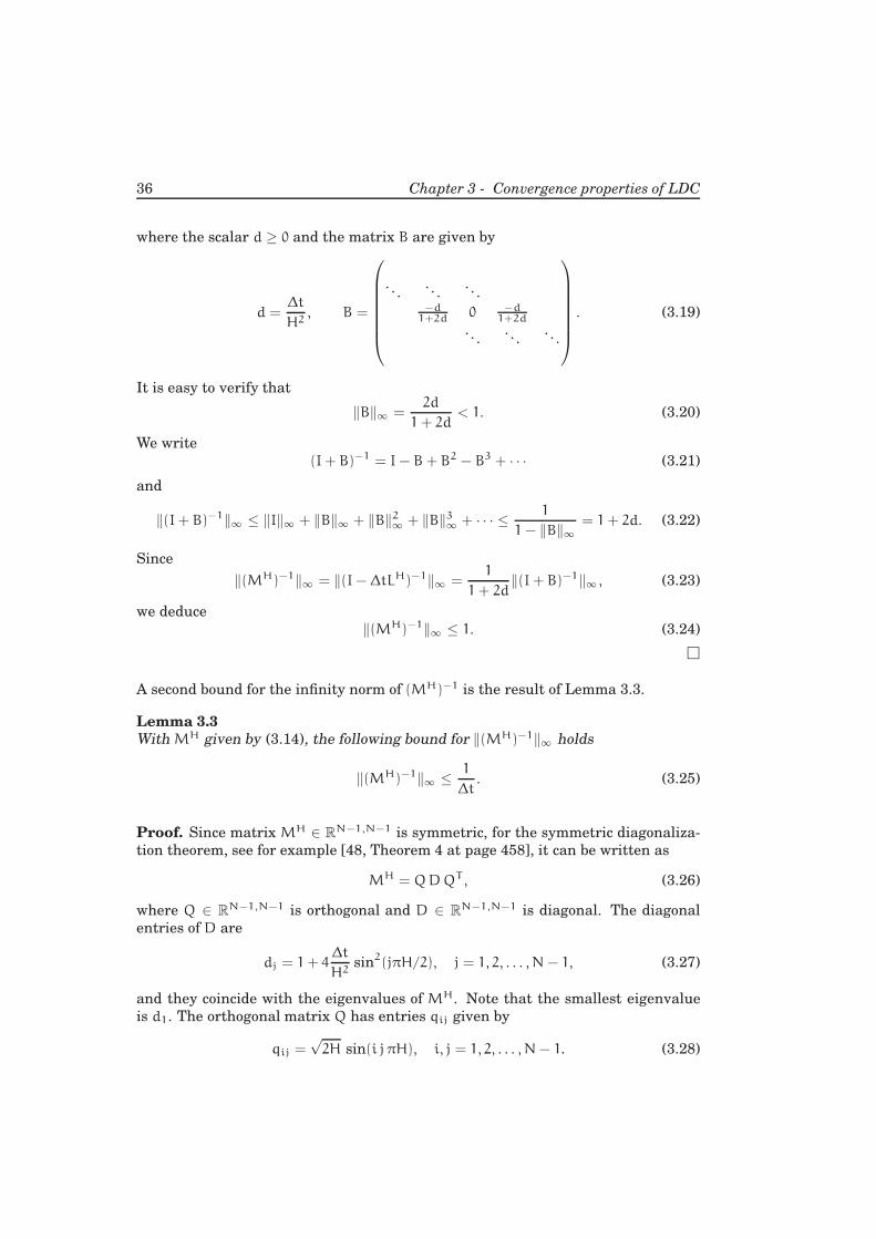
36 Chapter 3 - Convergence properties of LDC
where the scalar d ≥ 0 and the matrix B are given by
d =∆t
H2, B =
. . .. . .
. . .−d
1+2d0 −d
1+2d
. . .. . .
. . .
. (3.19)
It is easy to verify that
‖B‖∞ =2d
1+ 2d< 1. (3.20)
We write
(I+ B)−1 = I − B+ B2 − B3 + · · · (3.21)
and
‖(I+ B)−1‖∞ ≤ ‖I‖∞ + ‖B‖∞ + ‖B‖2∞ + ‖B‖3
∞ + · · · ≤ 1
1− ‖B‖∞= 1+ 2d. (3.22)
Since
‖(MH)−1‖∞ = ‖(I− ∆tLH)−1‖∞ =1
1+ 2d‖(I+ B)−1‖∞ , (3.23)
we deduce
‖(MH)−1‖∞ ≤ 1. (3.24)
A second bound for the infinity norm of (MH)−1 is the result of Lemma 3.3.
Lemma 3.3
With MH given by (3.14), the following bound for ‖(MH)−1‖∞ holds
‖(MH)−1‖∞ ≤ 1
∆t. (3.25)
Proof. Since matrix MH ∈ RN−1,N−1 is symmetric, for the symmetric diagonaliza-
tion theorem, see for example [48, Theorem 4 at page 458], it can be written as
MH = QDQT , (3.26)
where Q ∈ RN−1,N−1 is orthogonal and D ∈ R
N−1,N−1 is diagonal. The diagonal
entries of D are
dj = 1+ 4∆t
H2sin2
(jπH/2), j = 1, 2, . . . , N − 1, (3.27)
and they coincide with the eigenvalues of MH. Note that the smallest eigenvalue
is d1. The orthogonal matrix Q has entries qij given by
qij =√2H sin(i j πH), i, j = 1, 2, . . . , N− 1. (3.28)
3.2 A one-dimensional model problem 37
From (3.28) we note that Q is also symmetric. We can thus write
(MH)−1 = QD−1Q. (3.29)
It can easily be shown that
‖Q‖∞ = maxi
N−1∑
j=1
|qij|
≤ (N− 1)√2H, (3.30)
‖D−1Q‖∞ = maxi
1
di
N−1∑
j=1
|qij|
≤ (N − 1)√2H
1
d1
. (3.31)
We note that, since we chose the integer N > 1, then H = 1/N is such that 0 ≤ H ≤1/2. Using the following inequality
sin2
(
πH
2
)
≤ H, for 0 ≤ H ≤ 1/2, (3.32)
we can show that
1
d1
=1
1+ 4∆t/H2 sin2(πH/2)
≤ 1
1+ 4∆t/H≤ H
4∆t. (3.33)
Combination of (3.29), (3.30), (3.31) and (3.33) finally yields
‖(MH)−1‖∞ ≤ ‖Q‖∞ ‖D−1Q‖∞ ≤ (N− 1)22H2 1
4∆t≤ 1
∆t. (3.34)
Results of Lemmas 3.2 and 3.3 are illustrated in Figure 3.1, where ‖(MH)−1‖∞ is
plotted as a function of ∆t for two different values of the grid size H. Formula (3.16)
and the results of Lemma 3.2 and Lemma 3.3 are combined in Theorem 3.4.
Theorem 3.4
The following bound for ‖M1‖∞ holds
‖M1‖∞ ≤ min(1,1
∆t). (3.35)
Note that the bound provided by Theorem 3.4 is independent of H and thus it holds
for any choice of the coarse grid size.
3.2.2 The expression of the M2 infinity norm
In this section we find an expression for the infinity norm ofM2. We let gH,nΓ ∈ R be
the solution found at point x = γ by performing one time step ∆t on the coarse grid.
From the definition of M2, see (3.11), we have that
M2gH,nΓ = XH
l
(
BHl,Γg
H,nΓ +MH
l RH,hun
)
, (3.36)
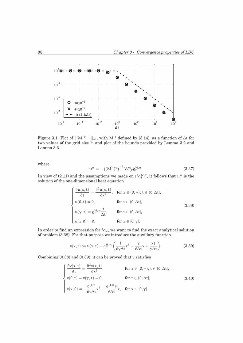
38 Chapter 3 - Convergence properties of LDC
10−6
10−4
10−2
100
102
104
106
10−6
10−4
10−2
100
∆ t
H=10−1
H=10−2
min(1,1/∆ t)
Figure 3.1: Plot of ‖(MH)−1‖∞ , with MH defined by (3.14), as a function of ∆t for
two values of the grid size H and plot of the bounds provided by Lemma 3.2 and
Lemma 3.3.
where
un = −(
(Mhl )τ)−1
Wnl,Γg
H,nΓ . (3.37)
In view of (2.11) and the assumptions we made on (Mhl )τ, it follows that un is the
solution of the one-dimensional heat equation
∂u(x, t)
∂t=∂2u(x, t)
∂x2, for x ∈ (0, γ), t ∈ (0, ∆t],
u(0, t) = 0, for t ∈ (0, ∆t],
u(γ, t) = gH,nΓ
t
∆t, for t ∈ (0, ∆t],
u(x, 0) = 0, for x ∈ [0, γ].
(3.38)
In order to find an expression for M2, we want to find the exact analytical solution
of problem (3.38). For that purpose we introduce the auxiliary function
v(x, t) := u(x, t) − gH,nΓ
(
1
6γ∆tx3 −
γ
6∆tx+
xt
γ∆t
)
. (3.39)
Combining (3.38) and (3.39), it can be proved that v satisfies
∂v(x, t)
∂t=∂2v(x, t)
∂x2, for x ∈ (0, γ), t ∈ (0, ∆t],
v(0, t) = v(γ, t) = 0, for t ∈ (0, ∆t],
v(x, 0) = −gH,n
Γ
6γ∆tx3 +
gH,nΓ γ
6∆tx, for x ∈ [0, γ].
(3.40)
3.2 A one-dimensional model problem 39
Problem (3.40) can be solved using the technique of separation of variables. We
express its solution in the form
v(x, t) =gH,n
Γ
∆t
∞∑
m=1
vme−m2π2t/γ2
sin
(
mπx
γ
)
, (3.41)
where the coefficients vm are to be computed from the initial condition
v(x, 0) =gH,n
Γ
∆t
∞∑
m=1
vm sin
(
mπx
γ
)
= −gH,n
Γ
6γ∆tx3 +
gH,nΓ γ
6∆tx. (3.42)
We find
vm =2
γ
∆t
gH,nΓ
∫γ
0
v(x, 0) dx = −2(−1)mγ2
m3π3. (3.43)
Using (3.41), the solution of the original problem (3.38) turns out to be
u(x, t) =gH,n
Γ
∆t
( ∞∑
m=1
vme−m2π2t/γ2
sin
(
mπx
γ
)
+1
6γx3 −
γ
6x+
xt
γ
)
. (3.44)
Solution (3.44) will now be used to express the productM2gH,nΓ .
Equation (3.36) states thatM2gH,nΓ equals the residual of the coarse grid discretiza-
tion scheme (centered differences and implicit Euler) applied to the function u(x, t)
for all grid points x ∈ ΩHdef. Taking already in account that u(x, 0) = 0, we have
M2gH,nΓ (x) = u(x, ∆t) −
∆t
H2(u(x +H,∆t) − 2u(x, ∆t) + u(x −H,∆t)) . (3.45)
We use the identity
sin
(
mπ(x+H)
γ
)
− 2 sin
(
mπx
γ
)
+ sin
(
mπ(x−H)
γ
)
= −4 sin
(
mπH
2γ
)
sin
(
mπx
γ
)
(3.46)
to combine (3.44) and (3.45) into
M2gH,nΓ (x) =
gH,nΓ
∆t
( ∞∑
m=1
vme−m2π2∆t/γ2
sin
(
mπx
γ
)
+1
6γx3 −
γ
6x
)
+4gH,n
Γ
H2
∞∑
m=1
vme−m2π2∆t/γ2
sin
(
mπH
2γ
)
sin
(
mπx
γ
)
.
(3.47)
Assuming that the function u is sufficiently smooth, another expression for the
product M2gH,nΓ (x) can be derived using Taylor expansions on the right hand side
of (3.45) and the fact that u satisfies the partial differential equation in (3.38). We
obtain
M2gH,nΓ (x) =
1
2
∂2u
∂t2
∣
∣
∣
(x,ϑ)∆t2 +
1
12
∂4u
∂x4
∣
∣
∣
(ξ,∆t)∆tH2, (3.48)
40 Chapter 3 - Convergence properties of LDC
with x − H < ξ < x + H and 0 < ϑ < ∆t. The time and spatial derivatives of u can
be computed differentiating term by term the series in (3.44). A sufficient condition
for this is that the resulting series are absolute convergent. We obtain
∂2u
∂t2
∣
∣
∣
(x,ϑ)=gH,n
Γ
∆t
2π
γ2
∞∑
m=1
(−1)mme−m2π2ϑ/γ2
sin
(
mπx
γ
)
, (3.49)
∂4u
∂x4
∣
∣
∣
(ξ,∆t)=gH,n
Γ
∆t
2π
γ2
∞∑
m=1
(−1)mme−m2π2∆t/γ2
sin
(
mπξ
γ
)
. (3.50)
Clearly the series on the right hand side of (3.49) and (3.50) are absolute convergent
for any positive ∆t and ϑ.
3.3 Iteration matrix norm asymptotics
With reference to the one-dimensional heat equation (3.12) and the settings illus-
trated in Section 3.2, in Section 3.3.1 we study the asymptotic expression of ‖Miter‖∞for ∆t ↓ 0, while in Section 3.3.2 we deal with Miter when ∆t → +∞. The limit case
∆t → +∞ corresponds to the stationary case limit; this is of interest in practical
applications when a time-dependent problem is solved to compute a stationary so-
lution.
3.3.1 The limit for small values of the time step ∆t
Combination of (3.9) with the result of Theorem 3.4 yields
‖Miter‖∞ ≤ ‖M1‖∞‖M2‖∞ ≤ ‖M2‖∞ , for ∆t < 1. (3.51)
As a consequence, in our analysis for ∆t ↓ 0 we will only consider the infinity norm
of M2. In particular, we will focus on the expression for M2 as given by (3.48).
In the perspective of studying ‖M2‖∞ for ∆t≪ 1, we first solve a preliminary prob-
lem. We introduce the following series (cf. (3.49) and (3.50))
Sx(ϑ) :=
∞∑
m=1
(−1)m sm sin(mπx
γ
)
, (3.52)
where
sm := me−m2ϑ, (3.53)
and we study the asymptotic behavior of Sx(ϑ) for ϑ ↓ 0 and fixed 0 < x < γ. Using
the fact that s−m = sm for all integers m, we rewrite (3.52) as
Sx(ϑ) = −1
2i
+∞∑
m=−∞me−m2ϑ e−imπ(x/γ−1). (3.54)
3.3 Iteration matrix norm asymptotics 41
If a function f(y) is sufficiently smooth, the following relation, which is known in
the literature (cf. for instance [59]) as Poisson summation formula, holds:
+∞∑
m=−∞f(m)e−imω =
+∞∑
k=−∞f(ω+ 2πk). (3.55)
The term f which appears in (3.55) is the Fourier transform of f(y), defined by
f(ω) :=
∫+∞
−∞f(y) e−iyω dy. (3.56)
For
f(y) = y e−y2ϑ, (3.57)
we have
f(ω) = − iπ1/2
2 ϑ3/2ωe−ω2/(4ϑ). (3.58)
Using Poisson summation formula, we can thus rewrite (3.54) as
Sx(ϑ) =π3/2
4 ϑ3/2
+∞∑
k=−∞
(
x
γ− 1+ 2k
)
exp
(
−π2(x/γ− 1+ 2k)2
4ϑ
)
. (3.59)
If we introduce the new variables
y :=1
2
(
1−x
γ
)
, α :=π2
ϑ, (3.60)
the original problem for Sx(ϑ) can be reformulated as follows: study the asymptotics
of
Ty(α) := −α3/2
2π3/2
+∞∑
k=−∞(k − y) e−α(k−y)2
(3.61)
for α→ +∞ and 0 < y < 1/2. For that, we need the results of the following lemma.
Lemma 3.5
The following identity holds:
limα→+∞
α
+∞∑
k=1
k2 e−kαβ = 0, β > 0. (3.62)
Proof. Note that by assumption β is positive. Starting from the identity
+∞∑
k=1
e−kαβ =e−αβ
1− e−αβ, α > 0, (3.63)
it can be easily shown that
α
+∞∑
k=1
k2 e−kαβ = αe−αβ(1+ e−αβ)
(1− e−αβ)3, α > 0. (3.64)
42 Chapter 3 - Convergence properties of LDC
Claim (3.62) follows immediately since the limit for α→ +∞ of the right hand side
of (3.64) is 0.
The result of Lemma 3.5 is used in the proof of Theorem 3.6, which provides the
asymptotic expression of Ty(α) for α→ +∞. First we introduce the following nota-
tion: we say that f(α) is asymptotically equivalent to g(α) for α→ α0 and we write
f(α) ≈ g(α), (α→ α0), (3.65)
if
limα→α0
f(α)
g(α)= 1. (3.66)
Theorem 3.6
The following equivalence holds:
Ty(α) ≈ 1
2π3/2α3/2 y e−αy2
, (α→ +∞), (3.67)
with 0 < y < 1/2.
Proof. For proving (3.67) it is sufficient to show (cf. (3.61)) that
limα→+∞
1
ye−αy2
+∞∑
k=−∞(k − y)e−α(k−y)2
= −1, with 0 < y < 1/2. (3.68)
The series in (3.68) can be written in a more convenient way as follows:
+∞∑
k=−∞(k− y)e−α(k−y)2
= −ye−αy2
+
+∞∑
k=1
(
(k − y)e−α(k−y)2
− (k + y)e−α(k+y)2)
= −ye−αy2
− y
+∞∑
k=1
(
e−α(k−y)2
+ e−α(k+y)2)
+
+∞∑
k=1
k(
e−α(k−y)2
− e−α(k+y)2)
= −ye−αy2
(
1+
+∞∑
k=1
e−αk2 (
e2αky + e−2αky)
−1
y
+∞∑
k=1
k e−αk2 (
e2αky − e−2αky)
)
.
(3.69)
We proceed showing that
limα→∞
+∞∑
k=1
e−αk2 (
e2αky + e−2αky)
= 0, 0 < y < 1/2, (3.70)
and
limα→∞
1
y
+∞∑
k=1
k e−αk2 (
e2αky − e−2αky)
= 0, 0 < y < 1/2. (3.71)
3.3 Iteration matrix norm asymptotics 43
We start from (3.70). We notice that all the terms of the series in (3.70) are positive.
The idea is thus to find an upper bound for the sum of the series which goes to 0
as α→ +∞. We write
0 ≤+∞∑
k=1
e−αk2(
e2αky + e−2αky)
≤ 2+∞∑
k=1
e−αk2
e2αky ≤ 2+∞∑
k=1
e−αke2αky
= 2
+∞∑
k=1
(
e−α(1−2y))k ≤ 2 e−α(1−2y)
1− e−α(1−2y).
(3.72)
Clearly, if 0 < y < 1/2, the last term in (3.72) goes to 0 for α→ +∞. This proves
equation (3.70).
We adopt a similar strategy for (3.71). Also in this case we deal with a series with
positive terms. First we consider the following inequality
e2αky − e−2αky =
∫+2αky
−2αky
eζ dζ ≤ 4α ky e2αky, (3.73)
and then we use it to find an upper bound for the sum of the series in (3.71). We
write
0 ≤ 1
y
+∞∑
k=1
k e−αk2(
e2αky − e−2αky)
≤ 4α+∞∑
k=1
k2 e−αk2
e2αky
≤ 4α+∞∑
k=1
k2 e−αke2αky = 4α
+∞∑
k=1
k2 e−kα(1−2y),
(3.74)
with 0 < y < 1/2. We know from Lemma 3.5 that the last term goes to 0 for α→ +∞.
This proves (3.71). Combination of (3.69), (3.70) and (3.71) proves (3.68) and hence
Claim (3.67).
If we adopt again the old variables x and ϑ, see (3.60), the result of Theorem 3.6 can
be rewritten as
Sx(ϑ) ≈ g(x, ϑ), (ϑ ↓ 0), (3.75)
with
g(x, ϑ) :=π3/2
4 ϑ3/2
(
1−x
γ
)
e−π2(1−x/γ)2/ϑ (3.76)
and 0 < x < γ. In Figure 3.2, g(x, ϑ) is plotted as a function of x for different values
of ϑ. Equivalence (3.75) is used in the proof of the following theorem.
Theorem 3.7
Sx(ϑ) has the following properties:
1) Sx(ϑ) goes exponentially to zero as ϑ ↓ 0;
2) Sx(ϑ) goes exponentially to zero as ϑ ↓ 0 non-uniformly on 0 < x < γ;
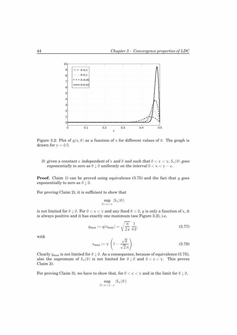
44 Chapter 3 - Convergence properties of LDC
0 0.1 0.2 0.3 0.4 0.5
0
1
2
3
4
5
6
7
8
9
10
x
ϑ=0.2
ϑ=0.1
ϑ=0.05
ϑ=0.02
Figure 3.2: Plot of g(x, ϑ) as a function of x for different values of ϑ. The graph is
drawn for γ = 0.5.
3) given a constant ǫ independent of x and ϑ and such that 0 < ǫ < γ, Sx(ϑ) goesexponentially to zero as ϑ ↓ 0 uniformly on the interval 0 < x < γ− ǫ.
Proof. Claim 1) can be proved using equivalence (3.75) and the fact that g goes
exponentially to zero as ϑ ↓ 0.
For proving Claim 2), it is sufficient to show that
sup0<x<γ
|Sx(ϑ)|
is not limited for ϑ ↓ 0. For 0 < x < γ and any fixed ϑ > 0, g is only a function of x, it
is always positive and it has exactly one maximum (see Figure 3.2), i.e.
gmax := g(xmax) =
√
π
2 e
1
4 ϑ, (3.77)
with
xmax := γ
(
1−
√ϑ√2π
)
. (3.78)
Clearly gmax is not limited for ϑ ↓ 0. As a consequence, because of equivalence (3.75),
also the supremum of Sx(ϑ) is not limited for ϑ ↓ 0 and 0 < x < γ. This proves
Claim 2).
For proving Claim 3), we have to show that, for 0 < ǫ < γ and in the limit for ϑ ↓ 0,
sup0<x<γ−ǫ
|Sx(ϑ)|
3.3 Iteration matrix norm asymptotics 45
remains limited. On the left of xmax, the function g is positive and monotonically
increasing (see again Figure 3.2). Moreover we note that
limϑ↓0
xmax = γ. (3.79)
Hence, for 0 < ǫ < γ, the following identity holds in the limit for ϑ ↓ 0
sup0<x<γ−ǫ
g(x, ϑ) = g(γ − ǫ, ϑ). (3.80)
The right hand side of (3.80) is limited for any positive value of ϑ and it goes to zero
as ϑ ↓ 0. Because of that and of equivalence (3.75), we deduce Claim 3).
At this point we have studied the properties of Sx(ϑ) for ϑ ↓ 0. The results found
for Sx(ϑ) are used to state the properties of ‖Miter‖∞ for ϑ ↓ 0.
Theorem 3.8
Consider the LDC method for the one-dimensional heat problem (3.12). Consider
the settings described in Section 3.2. In particular, let ΩH be a uniform coarsegrid with grid size H and, in ΩH, approximate the second space derivative by the
standard three-point finite differences scheme. Perform the temporal discretizationwith the backward Euler scheme and time step ∆t. Let the local region be Ωl =
(0, γ), with γ a multiple of H such that 0 < γ < 1. Locally replace the discretized
operator Mhl with the continuous operator (3.15). Moreover, let ǫ be a constant
independent of x and ϑ, and such that H < ǫ < γ. Finally, let ΩHdef , the subset ofΩH
l
in which an approximation of the local discretization error is computed, be given by
ΩHdef = (0, γ− ǫ) ∩ΩH
l . (3.81)
Then, the following results hold for ‖Miter‖∞ :
1) for any H ≥ 0, ‖Miter‖∞ goes exponentially to zero as ∆t ↓ 0;
2) for any H ≥ 0, ‖Miter‖∞ goes exponentially to zero as ∆t ↓ 0 uniformly onΩHdef .
Proof. For ∆t small enough, combination of (3.51) with (3.48), (3.49) and (3.50)
yields
‖Miter‖∞ ≤ ‖M2‖∞ ≤ π∆t
γ
∣
∣
∣
∣
Sx
(
π2 ϑ
γ2
)∣
∣
∣
∣
+π
6γ2
H2
∆t
∣
∣
∣
∣
Sξ
(
π2∆t
γ2
)∣
∣
∣
∣
, (3.82)
with x ∈ ΩHdef, x−H < ξ < x+H and 0 < ϑ < ∆t. Claims 1) and 2) follow immedi-
ately using the results of Theorem 3.7.
The fact that the norm of the iteration matrix goes to zero as ∆t ↓ 0 is very natural.
We expect this to happen in general and not only for the model problem considered
here. We explain this as follows: if the time step ∆t becomes extremely small, the
solution at the new time step becomes very close to the solution at the previous time
46 Chapter 3 - Convergence properties of LDC
level. In such a situation, there is little to be corrected in the approximation at the
new time step and, as a consequence, the LDC convergence rate is extremely fast.
As a final remark, we note that one basic assumption in the proof of Theorem 3.8 is
the use of a safety region. As discussed later in Sections 3.3.3 and 3.4, this assump-
tion is essential to have an exponential rate of convergence for∆t→ 0. Nevertheless,
the LDC method turns out to be convergent also if the extent of the safety region is
zero. This is similar to what happens in stationary cases. In [1, 4] the LDC iteration
error for a 2D Poisson problem is proved to reduce proportionally to H2 if ǫ > 0.
However, LDC is shown to be convergent (at a lower rate) also if ǫ = 0.
3.3.2 The stationary case limit
In the limit case ∆t → +∞, we expect the LDC convergence rate for the 1D heat
equation to be the same as the LDC convergence rate for the one-dimensional Pois-
son’s equation. When LDC is applied to a 1D Poisson problem in combination with
centered differences or any other method that integrates linear functions exactly,
the method reaches a fixed point in one iteration for any grid size H > 0. (If H = 0,
the stationary problem is solved exactly and there is no need to use LDC). This is
proved in [5] and means that, in such a case, the iteration matrix is zero.
In the following theorem we provide a bound for ‖Miter‖∞ that holds in the limit for
∆t→ +∞ and any grid size H > 0. Clearly our results for the one-dimensional heat
equation fit into the theory of LDC for 1D stationary problems.
Theorem 3.9
Consider the LDC method for the one-dimensional heat problem (3.12). Consider
the settings described in Section 3.2 and a grid size H > 0. Then, for any γ such that0 < γ < 1, there exists a constant C such that
‖Miter‖∞ ≤ C
∆t2, (∆t→ +∞). (3.83)
Proof. For ∆t > 1, combination of definition (3.9) with the result of Theorem 3.4
yields
‖Miter‖∞ ≤ 1
∆t‖M2‖∞ . (3.84)
Hence, for proving Theorem 3.9 it is sufficient to show that, for any γ ∈ (0, 1), there
exists a constant C such that
‖M2‖∞ ≤ C
∆t, (∆t→ +∞). (3.85)
We consider M2 as expressed by (3.47) and we write
‖M2(x)‖∞ ≤ ‖S1‖∞ + ‖S2‖∞ +∥
∥Spoly
∥
∥
∞ , (3.86)
3.3 Iteration matrix norm asymptotics 47
with
S1 :=1
∆t
∞∑
m=1
vme−m2π2∆t/γ2
sin
(
mπx
γ
)
, (3.87)
S2 :=4
H2
∞∑
m=1
vme−m2π2∆t/γ2
sin
(
mπH
2γ
)
sin
(
mπx
γ
)
, (3.88)
Spoly :=1
∆t
(
1
6γx3 −
γ
6x
)
. (3.89)
With vm given by (3.43), we prove that ‖S1‖∞ and ‖S2‖∞ are o(1/∆t), (∆t → +∞).
We start from S2. We write
‖S2‖∞ ≤ 4
H2
∞∑
m=1
|vm|
∣
∣
∣e−m2π2∆t/γ2∣
∣
∣
∣
∣
∣
∣
sin
(
mπH
2γ
)∣
∣
∣
∣
∥
∥
∥
∥
sin
(
mπx
γ
)∥
∥
∥
∥
∞
≤ 8γ2
π3H2
∞∑
m=1
∣
∣
∣e−mπ2∆t/γ2
∣
∣
∣ =8γ2
π3H2
e−π2∆t/γ2
1− e−π2∆t/γ2 .
(3.90)
For any H > 0 and any γ ∈ (0, 1), the last term in (3.90) is o(1/∆t), (∆t → +∞). A
similar procedure can be used to show that ‖S1‖∞ is o(1/∆t), (∆t → +∞). Having
proved that two of the terms on the right hand side of (3.86) are o(1/∆t), (∆t→ +∞),
we deal now with the third one. Clearly, with the assumptions made,∥
∥Spoly
∥
∥
∞ is
O(1/∆t), (∆t→ +∞). Therefore, there exists a constant C such that
∥
∥Spoly
∥
∥
∞ ≤ C
∆t, (∆t→ +∞). (3.91)
This completes our proof.
3.3.3 Plots of the iteration matrix norm
In Sections 3.3.1 and 3.3.2 we studied the asymptotic behavior of ‖Miter‖∞ for ∆t ↓ 0and ∆t→ +∞ and we found that, in both cases, the limit of ‖Miter‖∞ is zero. In
other words, we know two limit situations in which the rate of convergence of LDC
becomes extremely fast. This does not mean, however, that the LDC method always
converges. In this section we provide arguments in favor of the conjecture that, for
our model problem and settings, Miter is less than one for any choice of H and ∆t,
and thus the LDC method is unconditionally convergent.
For the one-dimensional heat equation and the LDC settings discussed in Sec-
tion 3.2, we can compute Miter ∈ R explicitly. For that we use the original defi-
nition (3.9) and we expressM1 by (3.10), with MH as in (3.14), and M2 by (3.47). In
Figure 3.3 we plot Miter as a function of ∆t for different values of H and for γ = 0.5.
In Figure 3.3-(a) Miter is computed with a safety region ǫ = 0.15, while in Fig-
ure 3.3-(b) no safety region is adopted. We immediately note that in both cases the
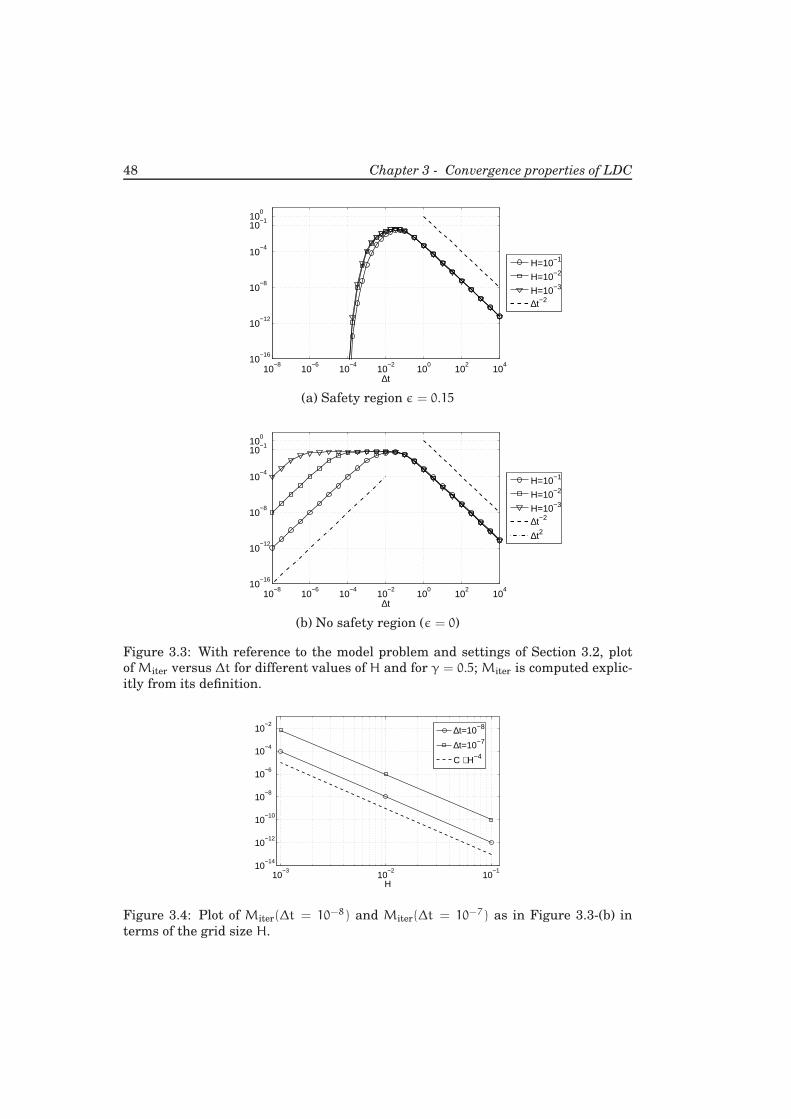
48 Chapter 3 - Convergence properties of LDC
10−8
10−6
10−4
10−2
100
102
104
10−16
10−12
10−8
10−4
10−1100
∆t
H=10−1
H=10−2
H=10−3
∆t−2
(a) Safety region ǫ = 0.15
10−8
10−6
10−4
10−2
100
102
104
10−16
10−12
10−8
10−4
10−1100
∆t
H=10−1
H=10−2
H=10−3
∆t−2
∆t2
(b) No safety region (ǫ = 0)
Figure 3.3: With reference to the model problem and settings of Section 3.2, plot
of Miter versus ∆t for different values of H and for γ = 0.5; Miter is computed explic-
itly from its definition.
10−3
10−2
10−1
10−14
10−12
10−10
10−8
10−6
10−4
10−2
H
∆t=10−8
∆t=10−7
C ⋅ H−4
Figure 3.4: Plot of Miter(∆t = 10−8) and Miter(∆t = 10−7) as in Figure 3.3-(b) in
terms of the grid size H.
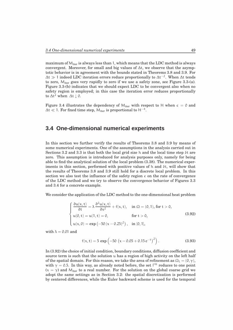
3.4 One-dimensional numerical experiments 49
maximum ofMiter is always less than 1, which means that the LDC method is always
convergent. Moreover, for small and big values of ∆t, we observe that the asymp-
totic behavior is in agreement with the bounds stated in Theorems 3.8 and 3.9. For
∆t ≫ 1 indeed LDC iteration errors reduce proportionally to ∆t−2. When ∆t tends
to zero, Miter goes very rapidly to zero if we use a safety zone, see Figure 3.3-(a).
Figure 3.3-(b) indicates that we should expect LDC to be convergent also when no
safety region is employed; in this case the iteration error reduces proportionally
to ∆t2 when ∆t ↓ 0.
Figure 3.4 illustrates the dependency of Miter with respect to H when ǫ = 0 and
∆t≪ 1. For fixed time step, Miter is proportional to H−4.
3.4 One-dimensional numerical experiments
In this section we further verify the results of Theorems 3.8 and 3.9 by means of
some numerical experiments. One of the assumptions in the analysis carried out in
Sections 3.2 and 3.3 is that both the local grid size h and the local time step δt are
zero. This assumption is introduced for analysis purposes only, namely for being
able to find the analytical solution of the local problem (3.38). The numerical exper-
iments in this section, performed with positive values of h and δt, will show that
the results of Theorems 3.8 and 3.9 still hold for a discrete local problem. In this
section we also test the influence of the safety region ǫ on the rate of convergence
of the LDC method and we try to observe the convergence behavior of Figures 3.3
and 3.4 for a concrete example.
We consider the application of the LDC method to the one-dimensional heat problem
∂u(x, t)
∂t= λ
∂2u(x, t)
∂x2+ f(x, t), in Ω = (0, 1), for t > 0,
u(0, t) = u(1, t) = 0, for t > 0,
u(x, 0) = exp(
−50 (x − 0.25)2)
, in [0, 1],
(3.92)
with λ = 0.01 and
f(x, t) = 5 exp(
−50(
x − 0.05 + 0.15 e−t)2)
. (3.93)
In (3.92) the choice of initial condition, boundary conditions, diffusion coefficient and
source term is such that the solution u has a region of high activity on the left half
of the spatial domain. For this reason, we take the area of refinement asΩl = (0, γ),
with γ = 0.5. In this way, as already noted before, the set ΓH reduces to one point
(x = γ) and Miter to a real number. For the solution on the global coarse grid we
adopt the same settings as in Section 3.2: the spatial discretization is performed
by centered differences, while the Euler backward scheme is used for the temporal
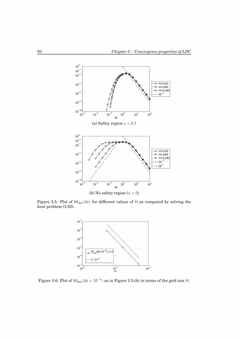
50 Chapter 3 - Convergence properties of LDC
10−6
10−4
10−2
100
102
104
10−10
10−8
10−6
10−4
10−2
10−1
100
∆t
H=1/20H=1/60H=1/180∆t−2
(a) Safety region ǫ = 0.1
10−6
10−4
10−2
100
102
104
10−10
10−8
10−6
10−4
10−2
10−1
100
∆t
H=1/20H=1/60H=1/180∆t−2
∆t2
(b) No safety region (ǫ = 0)
Figure 3.5: Plot of Miter(∆t) for different values of H as computed by solving the
heat problem (3.92).
10−3
10−2
10−1
10−7
10−6
10−5
10−4
10−3
10−2
H
Miter
(∆t=10−4), ε=0
C ⋅ H−4
Figure 3.6: Plot of Miter(∆t = 10−4) as in Figure 3.5-(b) in terms of the grid size H.
3.4 One-dimensional numerical experiments 51
discretization. For the solution on the local fine grid we employ the same numerical
schemes as on the global coarse grid.
We run tests aimed at measuring the convergence rate of the LDC method during
one time step. We adopt the following strategy: starting from the initial condition,
we perform one LDC time step with a chosen grid size H and a chosen time step ∆t.
The local grid size and time step are taken as h = H/5 and δt = ∆t/5. For measur-
ingMiter, we act as follows: at every LDC iteration, we store the coarse grid solution
on the interface ΓH. We say that the LDC iteration has converged when
|uH,1Γ,w − uH,1
Γ,w−1| < tolerance, (3.94)
for a certain w ≥ 1. In (3.94), uH,1Γ,w denotes the solution on ΓH after one time step
and w LDC iterations. In our numerical experiments, we set the value of the toler-
ance to 10−12. Once the converged value on the interface is known, the error eHΓ,w
can be computed for every iteration w that has been performed. Finally, see (3.7),
Miter is given by
Miter =eH
Γ,w
eHΓ,w−1
, (3.95)
for a certain w ≥ 1. In practice we take w = 1 in (3.95). Note that, if the LDC
method converges in exactly one iteration, Miter = 0.
We run two series of experiments on problem (3.92), the first one with a safety re-
gion, the second one with no safety region. The results are displayed in Figure 3.5.
In Figure 3.5-(a)Miter is plotted as a function of ∆t for different values of the coarse
grid size H. Except for the fact that the local problem is not solved analytically
but numerically, in this numerical experiment all the assumptions of Theorems 3.8
and 3.9 are satisfied. Note that the extent of the safety region (ǫ = 0.1) is greater
than H, for every H considered. As expected, Miter goes very rapidly to zero for
small values of ∆t while, for big values of the time step, iteration errors reduce pro-
portionally to ∆t−2. For each value ofH considered in the experiment, the maximum
ofMiter is always below 10−1; this means that, even in the worst case, the error eHΓ,w
is reduced by a factor bigger than 10 at every LDC iteration. Figure 3.5-(b) refers to
the experiment with no safety region. The behavior for ∆t≫ 1 is the same as before;
in Theorem 3.9, in fact, no assumption is made on the extent of ǫ. For ∆t≪ 1 itera-
tion errors reduce proportionally to ∆t2. Note that, also in this case, the maximum
of Miter is always below 10−1. Overall the graphs in Figure 3.5 are qualitatively
very similar to the ones in Figure 3.3, where Miter was computed directly from the
definition (3.9). In Figure 3.6 we finally plot, as a function of H, the values of Miter
as they are computed by solving problem (3.92) with ∆t = 10−4 and ǫ = 0. As al-
ready illustrated in Figure 3.4, with fixed (and small) ∆t and no safety region,Miter
is O(H−4).
So far we have only considered pure diffusion problems. Here we would also like
to investigate, by means of a numerical experiment, the LDC rate of convergence
when the method is applied to a one-dimensional convection-diffusion problem. We
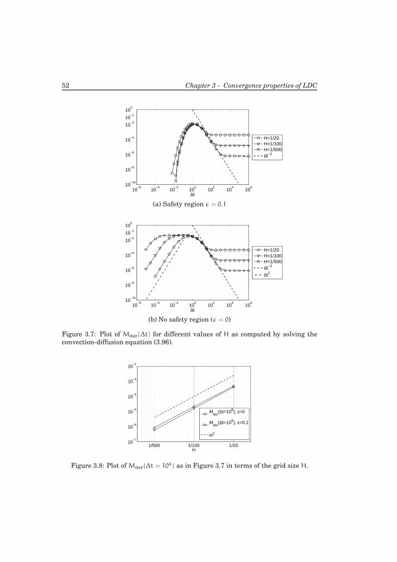
52 Chapter 3 - Convergence properties of LDC
10−6
10−4
10−2
100
102
104
106
10−10
10−8
10−6
10−4
10−2
10−1
100
∆t
H=1/20H=1/100H=1/500∆t−2
(a) Safety region ǫ = 0.1
10−6
10−4
10−2
100
102
104
106
10−10
10−8
10−6
10−4
10−2
10−1
100
∆t
H=1/20H=1/100H=1/500∆t−2
∆t2
(b) No safety region (ǫ = 0)
Figure 3.7: Plot of Miter(∆t) for different values of H as computed by solving the
convection-diffusion equation (3.96).
1/500 1/100 1/2010
−7
10−6
10−5
10−4
10−3
10−2
H
Miter
(∆t=106), ε=0
Miter
(∆t=106), ε=0.1
H2
Figure 3.8: Plot of Miter(∆t = 106) as in Figure 3.7 in terms of the grid size H.

3.5 Two-dimensional numerical experiments 53
consider the following partial differential equation
∂u(x, t)
∂t+ v
∂u(x, t)
∂x= λ
∂2u(x, t)
∂x2+ f(x, t), in Ω = (0, 1), for t > 0, (3.96)
with v = −0.1. Equation (3.96) is solved with the same initial condition, boundary
conditions, diffusion coefficient and source term as problem (3.92). The convection
and the diffusion term are discretized by second-order centered differences, while
the time discretization is performed by the backward Euler scheme. Moreover the
same local region is adopted as before, and the same strategy to compute Miter is
employed. Note that in (3.96) convection is the main way of heat transport since the
relative weight of convection with respect to diffusion is
|v|
λ=0.1
0.01= 10. (3.97)
Like before, we run two sets of numerical experiments, one with a safety region
ǫ = 0.1 and another one with no safety region. The results are displayed in Fig-
ure 3.7. For small values of the time step ∆t the rate of convergence Miter has the
same behavior as for pure diffusion problems. Also the maximum value of Miter(∆t)
is, for every H, about the same (less than 10−1) as observed before. For big values
of ∆t, however, we note thatMiter first decreases as O(∆t−2), but then an asymptotic
value (greater than 0) is reached. To illustrate the dependency of the asymptotic
value on the grid size, in Figure 3.8 we plot, as a function of H, Miter(∆t = 106) as
computed in the two sets of experiments on problem (3.96). From the graph we can
see that, in both cases, the asymptotic value is proportional to the square of the
coarse grid size.
3.5 Two-dimensional numerical experiments
In this section we would like to study the convergence properties of LDC for two-
dimensional parabolic partial differential equations experimentally. We will con-
sider both a pure diffusion and a convection-diffusion problem. Like before, our goal
is to measure the convergence rate of LDC during one time step. We note that in
2D Miter is indeed a matrix: its dimension, see (3.8), coincides with the number of
coarse grid points in ΓH.
We start considering the two-dimensional heat problem
∂u
∂t= λ∇2u+ f, in Ω = (0, 1)2, for t > 0,
u = 0, on ∂Ω, for t > 0,
u = exp(
−20(
(x − 0.3)2
+ (y− 0.3)2))
, in Ω,
(3.98)
with λ = 10−2 and
f = exp(
−40(
(
x− 0.2 − 0.15e−t)2
+(
y− 0.2 − 0.15e−t)2))
. (3.99)
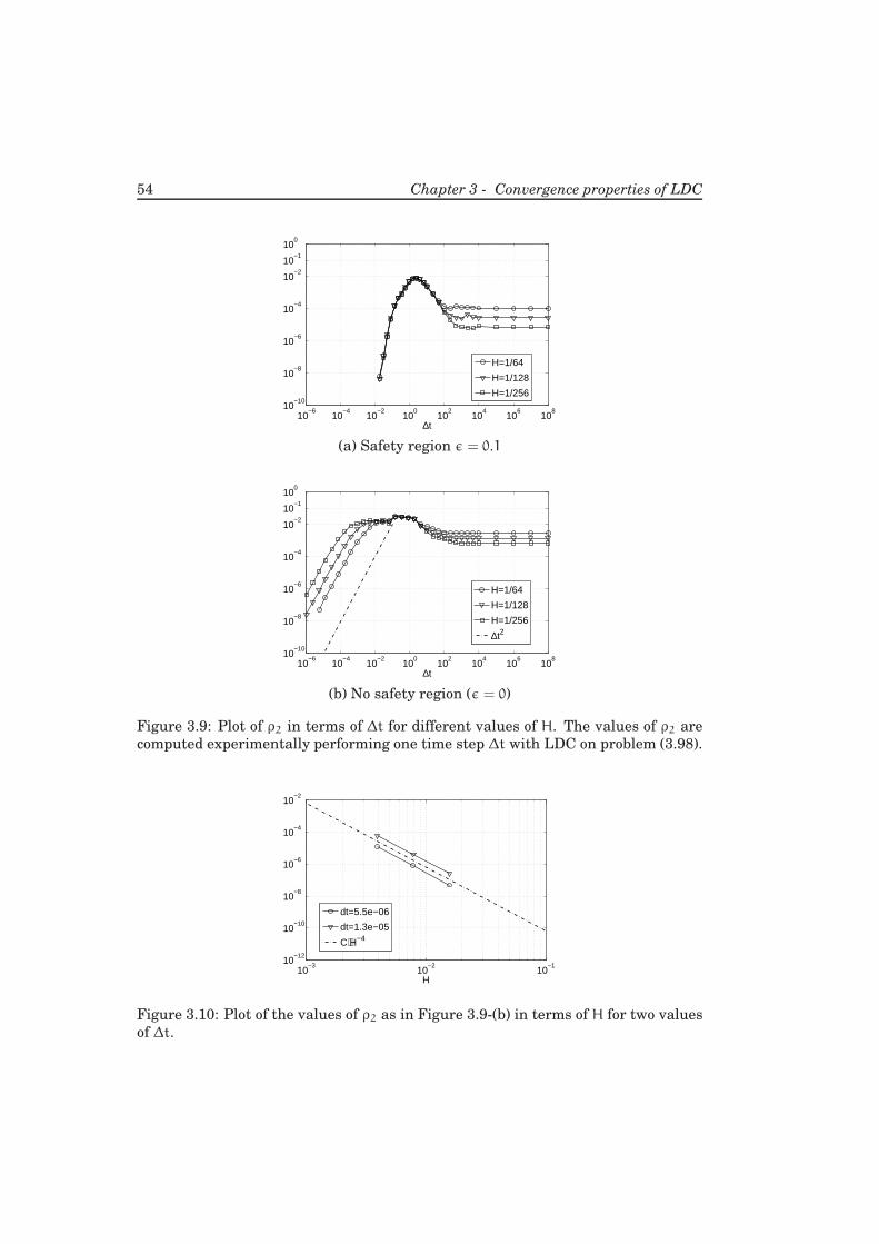
54 Chapter 3 - Convergence properties of LDC
10−6
10−4
10−2
100
102
104
106
108
10−10
10−8
10−6
10−4
10−2
10−1
100
∆t
H=1/64
H=1/128
H=1/256
(a) Safety region ǫ = 0.1
10−6
10−4
10−2
100
102
104
106
108
10−10
10−8
10−6
10−4
10−2
10−1
100
∆t
H=1/64
H=1/128
H=1/256
∆t2
(b) No safety region (ǫ = 0)
Figure 3.9: Plot of ρ2 in terms of ∆t for different values of H. The values of ρ2 are
computed experimentally performing one time step ∆t with LDC on problem (3.98).
10−3
10−2
10−1
10−12
10−10
10−8
10−6
10−4
10−2
H
dt=5.5e−06
dt=1.3e−05
C⋅H−4
Figure 3.10: Plot of the values of ρ2 as in Figure 3.9-(b) in terms of H for two values
of ∆t.
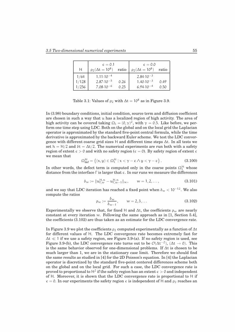
3.5 Two-dimensional numerical experiments 55
ǫ = 0.1 ǫ = 0.0
H ρ2(∆t = 108) ratio ρ2(∆t = 108) ratio
1/64 1.11·10−4 2.84·10−3
1/128 2.87·10−5 0.26 1.40·10−3 0.49
1/256 7.08·10−6 0.25 6.94·10−4 0.50
Table 3.1: Values of ρ2 with ∆t = 108 as in Figure 3.9.
In (3.98) boundary conditions, initial condition, source term and diffusion coefficient
are chosen in such a way that u has a localized region of high activity. The area of
high activity can be covered taking Ωl = (0, γ)2, with γ = 0.5. Like before, we per-
form one time step using LDC. Both on the global and on the local grid the Laplacian
operator is approximated by the standard five-point central formula, while the time
derivative is approximated by the backward Euler scheme. We test the LDC conver-
gence with different coarse grid sizes H and different time steps ∆t. In all tests we
set h = H/2 and δt = ∆t/2. The numerical experiments are run both with a safety
region of extent ǫ > 0 and with no safety region (ǫ = 0). By safety region of extent ǫ
we mean that
ΩHdef =
(x, y) ∈ ΩH
l | x < γ− ǫ∧ y < γ− ǫ. (3.100)
In other words, the defect term is computed only in the coarse points ΩHl whose
distance from the interface Γ is larger that ǫ. In our runs we measure the differences
δw := ‖uH,nΓ,w − uH,n
Γ,w−1‖∞ , w = 1, 2, . . . , (3.101)
and we say that LDC iteration has reached a fixed point when δw < 10−12. We also
compute the ratios
ρw :=δw
δw−1
, w = 2, 3, . . . (3.102)
Experimentally we observe that, for fixed H and ∆t, the coefficients ρw are nearly
constant at every iteration w. Following the same approach as in [1, Section 5.4],
the coefficients (3.102) are thus taken as an estimate for the LDC convergence rate.
In Figure 3.9 we plot the coefficients ρ2 computed experimentally as a function of ∆t
for different values of H. The LDC convergence rate becomes extremely fast for
∆t ≪ 1 if we use a safety region, see Figure 3.9-(a). If no safety region is used, see
Figure 3.9-(b), the LDC convergence rate turns out to be O(∆t−2), (∆t → 0). This
is the same behavior observed for one-dimensional problems. If ∆t is chosen to be
much larger than 1, we are in the stationary case limit. Therefore we should find
the same results as studied in [4] for the 2D Poisson’s equation. In [4] the Laplacian
operator is discretized by the standard five-point centered differences scheme both
on the global and on the local grid. For such a case, the LDC convergence rate is
proved to proportional toH2 if the safety region has an extent ǫ > 0 and independent
of H. Moreover, it is shown that the LDC convergence rate is proportional to H if
ǫ = 0. In our experiments the safety region ǫ is independent of H and ρ2 reaches an
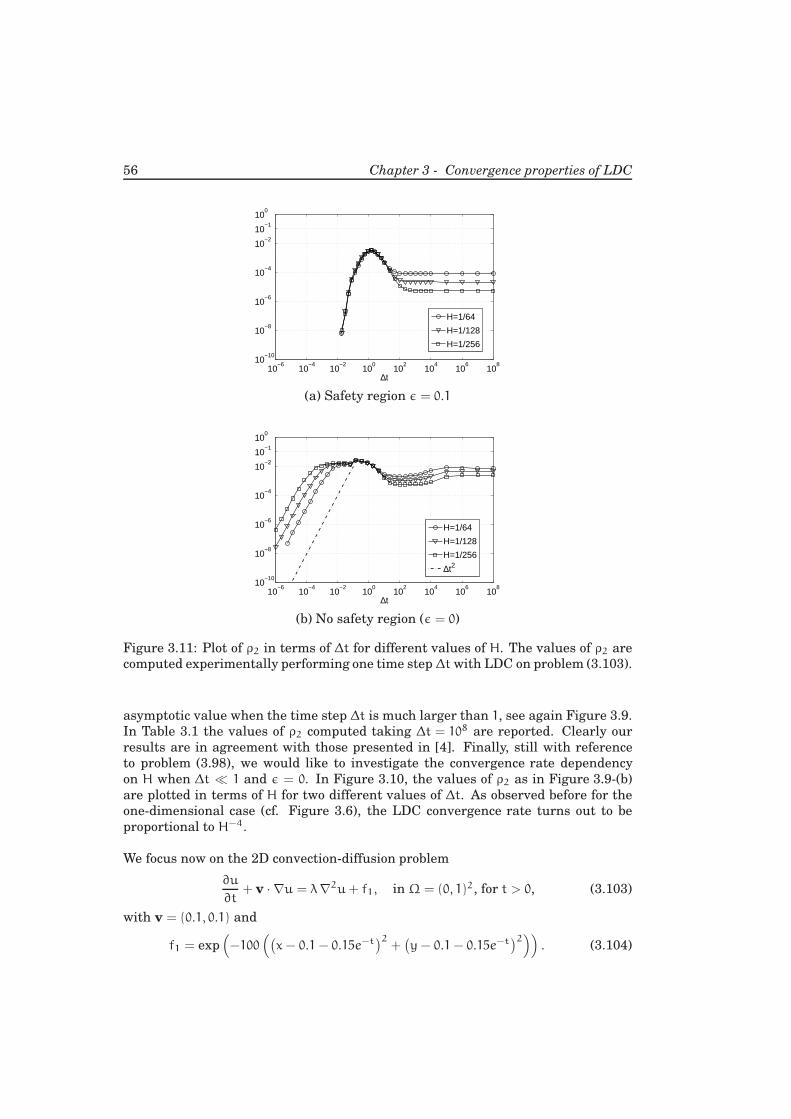
56 Chapter 3 - Convergence properties of LDC
10−6
10−4
10−2
100
102
104
106
108
10−10
10−8
10−6
10−4
10−2
10−1
100
∆t
H=1/64
H=1/128
H=1/256
(a) Safety region ǫ = 0.1
10−6
10−4
10−2
100
102
104
106
108
10−10
10−8
10−6
10−4
10−2
10−1
100
∆t
H=1/64
H=1/128
H=1/256
∆t2
(b) No safety region (ǫ = 0)
Figure 3.11: Plot of ρ2 in terms of ∆t for different values of H. The values of ρ2 are
computed experimentally performing one time step ∆twith LDC on problem (3.103).
asymptotic value when the time step ∆t is much larger than 1, see again Figure 3.9.
In Table 3.1 the values of ρ2 computed taking ∆t = 108 are reported. Clearly our
results are in agreement with those presented in [4]. Finally, still with reference
to problem (3.98), we would like to investigate the convergence rate dependency
on H when ∆t ≪ 1 and ǫ = 0. In Figure 3.10, the values of ρ2 as in Figure 3.9-(b)
are plotted in terms of H for two different values of ∆t. As observed before for the
one-dimensional case (cf. Figure 3.6), the LDC convergence rate turns out to be
proportional to H−4.
We focus now on the 2D convection-diffusion problem
∂u
∂t+ v · ∇u = λ∇2u+ f1, in Ω = (0, 1)2, for t > 0, (3.103)
with v = (0.1, 0.1) and
f1 = exp(
−100(
(
x− 0.1− 0.15e−t)2
+(
y− 0.1− 0.15e−t)2))
. (3.104)
3.5 Two-dimensional numerical experiments 57
ǫ = 0.1 ǫ = 0.0
H ρ2(∆t = 108) ratio ρ2(∆t = 108) ratio
1/64 8.18·10−5 7.66·10−3
1/128 2.18·10−5 0.27 4.80·10−3 0.63
1/256 5.34·10−6 0.25 2.42·10−3 0.50
Table 3.2: Values of ρ2 with ∆t = 108 as in Figure 3.11.
The diffusion coefficient λ, the boundary conditions and the initial condition are
the same as for the pure diffusion problem (3.98). Also in this case the solution u
has a local region of high activity that can be covered by taking Ωl = (0, γ)2, with
γ = 0.5. We adopt the same discretization schemes as in the previous experiment
and we discretize the convection term by second-order centered differences both on
the coarse and on the fine grid. In all tests the local problem is solved taking h = H/2
and δt = ∆t/2. We run the same kind of experiments as before and we show the
results in Figure 3.11. Once more we observe that the rate of convergence of LDC
goes extremely fast to zero for ∆t → 0 if we use a safety region, see Figure 3.11-(a).
Also in this case the LDC convergence rate is proportional to∆t−2 for∆t→ 0 if ǫ = 0,
see Figure 3.11-(b). In the stationary case limit ρ2 reaches an asymptotic value
which depends on H. The values of ρ2 computed for ∆t = 108 are listed in Table 3.2.
From the table we can see the same kind of results as for the pure diffusion problem.
We finally note that the plot of ρ2 as a function of H for ∆t ≪ 1 and ǫ = 0 would be
qualitatively similar to Figure 3.10: also for a 2D convection-diffusion problem the
LDC convergence rate is proportional to H−4 when ∆t≪ 1 and ǫ = 0.
In conclusion, the analysis and the numerical experiments presented in this chapter
show that the LDC method for time dependent-problems has very good convergence
properties. In fact LDC turns out to be convergent for any choice of the time step ∆t.
The rate of convergence of LDC can be improved by decreasing ∆t or by computing
the defect term using a safety region ǫ > H. For small values of the time step, the
convergence behavior of LDC is the same for one- and two-dimensional problems,
for pure diffusion and convection-diffusion equations.

Chapter 4
A finite volume adapted LDCmethod
In this chapter we apply the time-dependent LDC technique in combination with
standard finite volume discretizations on the global and local grid. Unlike in Chap-
ter 2, where the local grid is adaptively placed at each time step where the high
activity occurs, we assume that the high activity of the solution is always located, at
each time level, in the same (limited) part of the global domain. Already for this sim-
ple situation, the LDC method as presented in Chapter 2 is such that the discrete
conservation law, which is one of the main attractive features of the finite volume
method, does not necessarily hold for the solution on the composite grid. Here, we
introduce a finite volume adapted LDC method for parabolic problems for which the
conservation property is preserved.
In [6] a finite volume adapted LDC algorithm which is conservative on the compos-
ite grid is presented for elliptic problems. The main idea there is that the defect
correction should be such that the integrated fluxes across the interface between
the coarse and fine grid are balanced. In the time-dependent case we consider here,
we extend that idea and write the defect term in such a way that the balance across
the interface holds at every time level. In doing so we deal with the complication
that the time integration might be performed with different time steps on the global
and local grid.
In general, when finite volume discretizations are combined with local grid refine-
ment special care has to be taken to guarantee discrete conservation across the
interface between coarse and fine regions. This is a popular topic in the litera-
ture. In [39], for example, conservative cell-centered approximations on rectangu-
lar locally refined grids are derived for second order convection-diffusion equations.
In [21, 40] a posteriori error estimates are given for locally refined finite volume dis-
60 Chapter 4 - A finite volume adapted LDC method
cretizations of convection-diffusion-reaction equations. In [7] the focus is on high or-
der approximations and a fourth-order accurate finite volume based technique with
local refinement is proposed for Poisson’s equation; the method preserves discrete
conservation. Parabolic partial differential equations are treated in [51], where a
conservative adaptive strategy is proposed for the computation of fluxes at the in-
terfaces of locally nested grids. In [17] the features of a solver for compressible
flows and fluid-structure interaction are discussed; the solver integrates dynamic
adaptation, mesh generation and finite volume discretization.
The method and the results of this chapter have been previously presented in [45].
4.1 Problem formulation and initialization of LDC
In order to present the LDC method for parabolic problems in combination with
a finite volume discretization, we consider a two-dimensional convection-diffusion
equation for a quantity ϕ = ϕ(x, t). The equation can be expressed in integral for-
mulation as follows
∂
∂t
∫
V
ϕdΩ+
∫
∂V
(ϕv − λ∇ϕ) · n dγ =
∫
V
sdΩ in Θ, for all V ⊂ Ω, (4.1)
where v = v(x, t) is a given velocity field, λ = λ(x, t) > 0 is a diffusion coefficient
and s = s(x, t) is a known source term. Furthermore Θ is the time interval (0, tend],
while V is a generic volume contained in the spatial domainΩ := (0, xmax)×(0, ymax).
With ∂V we indicate the boundary of V and with n the outward unit vector perpen-
dicular to ∂V . We also introduce ∂Ω, the boundary ofΩ, and we define Ω := Ω∪∂Ω.
We close problem (4.1) by prescribing the Dirichlet boundary condition
ϕ = ψ, on ∂Ω×Θ, (4.2)
and the initial condition
ϕ(x, 0) = η, in Ω. (4.3)
In (4.2) and (4.3), ψ = ψ(x, t) and η = η(x) are given functions. We just consider
Dirichlet boundary conditions for simplicity, but the LDC method we are going to
describe can easily handle other types of boundary conditions, such as Neumann
or Robin. If all the variables in (4.1) are sufficiently smooth and the velocity field
is divergence free (∇ · v = 0), the integral formulation (4.1) is equivalent to the
differential formulation
∂ϕ
∂t+ v · ∇ϕ− ∇ · (λ∇ϕ) = s in Ω×Θ. (4.4)
We introduce the flux vector f by
f = f(ϕ) =
(
fx
fy
)
:= ϕv − λ∇ϕ, (4.5)
4.1 Problem formulation and initialization of LDC 61
so that equation (4.1) can be rewritten as
∂
∂t
∫
V
ϕdΩ+
∫
∂V
f · n dγ =
∫
V
sdΩ in Θ, for all V ⊂ Ω. (4.6)
We assume that ϕ, the continuous solution of (4.6) that satisfies (4.2) and (4.3), at
each time in Θ presents a region of high activity that covers a (small) part of Ω.
4.1.1 Composite grid definition
Problem (4.6) is first discretized in space on a global uniform coarse grid using the
finite volume method. We consider, in particular, a standard vertex-centered ap-
proach. This is just for notational convenience and the usage of other approaches,
e.g. cell-centered discretization, would guarantee the same properties in the method
we are describing. We introduce the grid size parameters Hx = xmax/Nx and Hy =
ymax/Ny, where Nx and Ny are positive integers, and the grid points
(xi, yj) := (iHx, jHy), i = 0, 1, . . . , Nx, j = 0, 1, . . . , Ny, (4.7)
(xi+1/2, yj) := ((i + 1/2)Hx, jHy), i = 0, 1, . . . , Nx − 1, j = 0, 1, . . . , Ny, (4.8)
(xi, yj+1/2) := (iHx, (j+ 1/2)Hy), i = 0, 1, . . . , Nx, j = 0, 1, . . . , Ny − 1. (4.9)
We define
ΩH := (xi, yj) ∩ Ω, ∂ΩH := ΩH ∩ ∂Ω, ΩH := ΩH \ ∂ΩH. (4.10)
We want to compute a discrete approximation ofϕ at the points of the computational
grid ΩH. Each point of ΩH is the center of a control volume
Vi,j := (xi−1/2, xi+1/2) × (yj−1/2, yj+1/2). (4.11)
The midpoints of the interfaces of volumes Vi,j form a dual grid
VH :=(
(xi+1/2, yj) ∪ (xi, yj+1/2))
∩Ω, (4.12)
on which we will define discrete fluxes. Figure 4.1 represents the global coarse
grid we have introduced in Ω. The figure is drawn for Nx = 5 and Ny = 7; grid
pointsΩH are marked with a circle, while rhombi and small squares identify points
of ∂ΩH and VH respectively.
We denote by G(ΩH), G(ΩH) and G(VH), the space of grid functions that operate
on ΩH, ΩH and VH respectively. We introduce the following notation: for a cer-
tain TH ∈ G(ΩH), we write TH = (THi,j), i = 1, 2, . . . , Nx − 1, j = 1, 2, . . . , Ny − 1, with
THi,j := TH(xi, yj). Similarly it is done for elements in G(ΩH) and G(VH). Given a cer-
tain FH ∈ G(VH), we introduce the central difference operator ∇HΣ : G(VH)→ G(ΩH)
by
(∇HΣ F
H)i,j := FHi,j+1/2 − FH
i,j−1/2 + FHi+1/2,j − FH
i−1/2,j. (4.13)
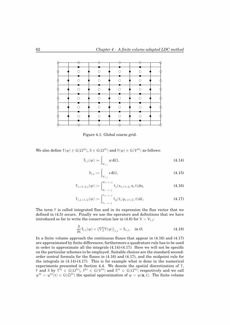
62 Chapter 4 - A finite volume adapted LDC method
Figure 4.1: Global coarse grid.
We also define T(ϕ) ∈ G(ΩH), S ∈ G(ΩH) and F(ϕ) ∈ G(VH) as follows:
Ti,j(ϕ) :=
∫
Vi,j
ϕdΩ, (4.14)
Si,j :=
∫
Vi,j
sdΩ, (4.15)
Fi+1/2,j(ϕ) :=
∫yj+1/2
yj−1/2
fx(xi+1/2, η, t)dη, (4.16)
Fi,j+1/2(ϕ) :=
∫xi+1/2
xi−1/2
fy(ξ, yj+1/2, t)dξ. (4.17)
The term F is called integrated flux and in its expression the flux vector that we
defined in (4.5) occurs. Finally we use the operators and definitions that we have
introduced so far to write the conservation law in (4.6) for V = Vi,j:
∂
∂tTi,j(ϕ) +
(
∇HΣ F(ϕ)
)
i,j= Si,j, in Θ. (4.18)
In a finite volume approach the continuous fluxes that appear in (4.16) and (4.17)
are approximated by finite differences; furthermore a quadrature rule has to be used
in order to approximate all the integrals (4.14)-(4.17). Here we will not be specific
on the particular schemes to be employed. Suitable choices are the standard second-
order central formula for the fluxes in (4.16) and (4.17), and the midpoint rule for
the integrals in (4.14)-(4.17). This is for example what is done in the numerical
experiments presented in Section 4.4. We denote the spatial discretization of T ,
F and S by TH ∈ G(ΩH), FH ∈ G(VH) and SH ∈ G(ΩH) respectively and we call
ϕH = ϕH(t) ∈ G(ΩH) the spatial approximation of ϕ = ϕ(x, t). The finite volume
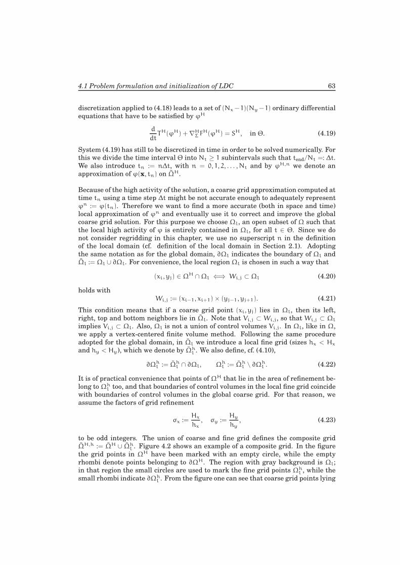
4.1 Problem formulation and initialization of LDC 63
discretization applied to (4.18) leads to a set of (Nx −1)(Ny −1) ordinary differential
equations that have to be satisfied by ϕH
d
dtTH(ϕH) + ∇H
Σ FH(ϕH) = SH, in Θ. (4.19)
System (4.19) has still to be discretized in time in order to be solved numerically. For
this we divide the time interval Θ into Nt ≥ 1 subintervals such that tend/Nt =: ∆t.
We also introduce tn := n∆t, with n = 0, 1, 2, . . . , Nt and by ϕH,n we denote an
approximation of ϕ(x, tn) on ΩH.
Because of the high activity of the solution, a coarse grid approximation computed at
time tn using a time step ∆t might be not accurate enough to adequately represent
ϕn := ϕ(tn). Therefore we want to find a more accurate (both in space and time)
local approximation of ϕn and eventually use it to correct and improve the global
coarse grid solution. For this purpose we choose Ωl, an open subset of Ω such that
the local high activity of ϕ is entirely contained in Ωl, for all t ∈ Θ. Since we do
not consider regridding in this chapter, we use no superscript n in the definition
of the local domain (cf. definition of the local domain in Section 2.1). Adopting
the same notation as for the global domain, ∂Ωl indicates the boundary of Ωl and
Ωl := Ωl ∪ ∂Ωl. For convenience, the local regionΩl is chosen in such a way that
(xi, yj) ∈ ΩH ∩Ωl ⇐⇒ Wi,j ⊂ Ωl (4.20)
holds with
Wi,j := (xi−1, xi+1) × (yj−1, yj+1). (4.21)
This condition means that if a coarse grid point (xi, yj) lies in Ωl, then its left,
right, top and bottom neighbors lie in Ωl. Note that Vi,j ⊂ Wi,j, so that Wi,j ⊂ Ωl
implies Vi,j ⊂ Ωl. Also, Ωl is not a union of control volumes Vi,j. In Ωl, like in Ω,
we apply a vertex-centered finite volume method. Following the same procedure
adopted for the global domain, in Ωl we introduce a local fine grid (sizes hx < Hx
and hy < Hy), which we denote by Ωhl . We also define, cf. (4.10),
∂Ωhl := Ωh
l ∩ ∂Ωl, Ωhl := Ωh
l \ ∂Ωhl . (4.22)
It is of practical convenience that points of ΩH that lie in the area of refinement be-
long to Ωhl too, and that boundaries of control volumes in the local fine grid coincide
with boundaries of control volumes in the global coarse grid. For that reason, we
assume the factors of grid refinement
σx :=Hx
hx
, σy :=Hy
hy
, (4.23)
to be odd integers. The union of coarse and fine grid defines the composite grid
ΩH,h := ΩH ∪ Ωhl . Figure 4.2 shows an example of a composite grid. In the figure
the grid points in ΩH have been marked with an empty circle, while the empty
rhombi denote points belonging to ∂ΩH. The region with gray background is Ωl;
in that region the small circles are used to mark the fine grid points Ωhl , while the
small rhombi indicate ∂Ωhl . From the figure one can see that coarse grid points lying
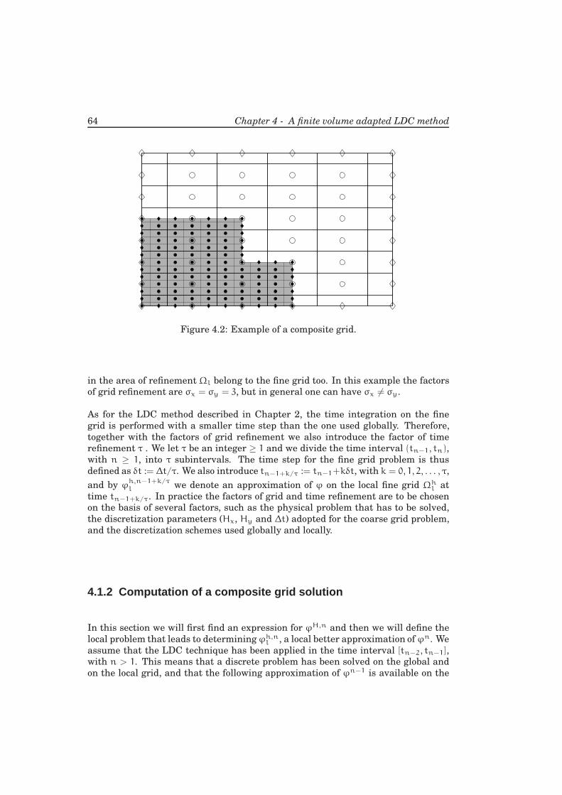
64 Chapter 4 - A finite volume adapted LDC method
Figure 4.2: Example of a composite grid.
in the area of refinement Ωl belong to the fine grid too. In this example the factors
of grid refinement are σx = σy = 3, but in general one can have σx 6= σy.
As for the LDC method described in Chapter 2, the time integration on the fine
grid is performed with a smaller time step than the one used globally. Therefore,
together with the factors of grid refinement we also introduce the factor of time
refinement τ . We let τ be an integer ≥ 1 and we divide the time interval (tn−1, tn),
with n ≥ 1, into τ subintervals. The time step for the fine grid problem is thus
defined as δt := ∆t/τ. We also introduce tn−1+k/τ := tn−1+kδt, with k = 0, 1, 2, . . . , τ,
and by ϕh,n−1+k/τ
l we denote an approximation of ϕ on the local fine grid Ωhl at
time tn−1+k/τ. In practice the factors of grid and time refinement are to be chosen
on the basis of several factors, such as the physical problem that has to be solved,
the discretization parameters (Hx, Hy and ∆t) adopted for the coarse grid problem,
and the discretization schemes used globally and locally.
4.1.2 Computation of a composite grid solution
In this section we will first find an expression for ϕH,n and then we will define the
local problem that leads to determiningϕh,nl , a local better approximation ofϕn. We
assume that the LDC technique has been applied in the time interval [tn−2, tn−1],
with n > 1. This means that a discrete problem has been solved on the global and
on the local grid, and that the following approximation of ϕn−1 is available on the
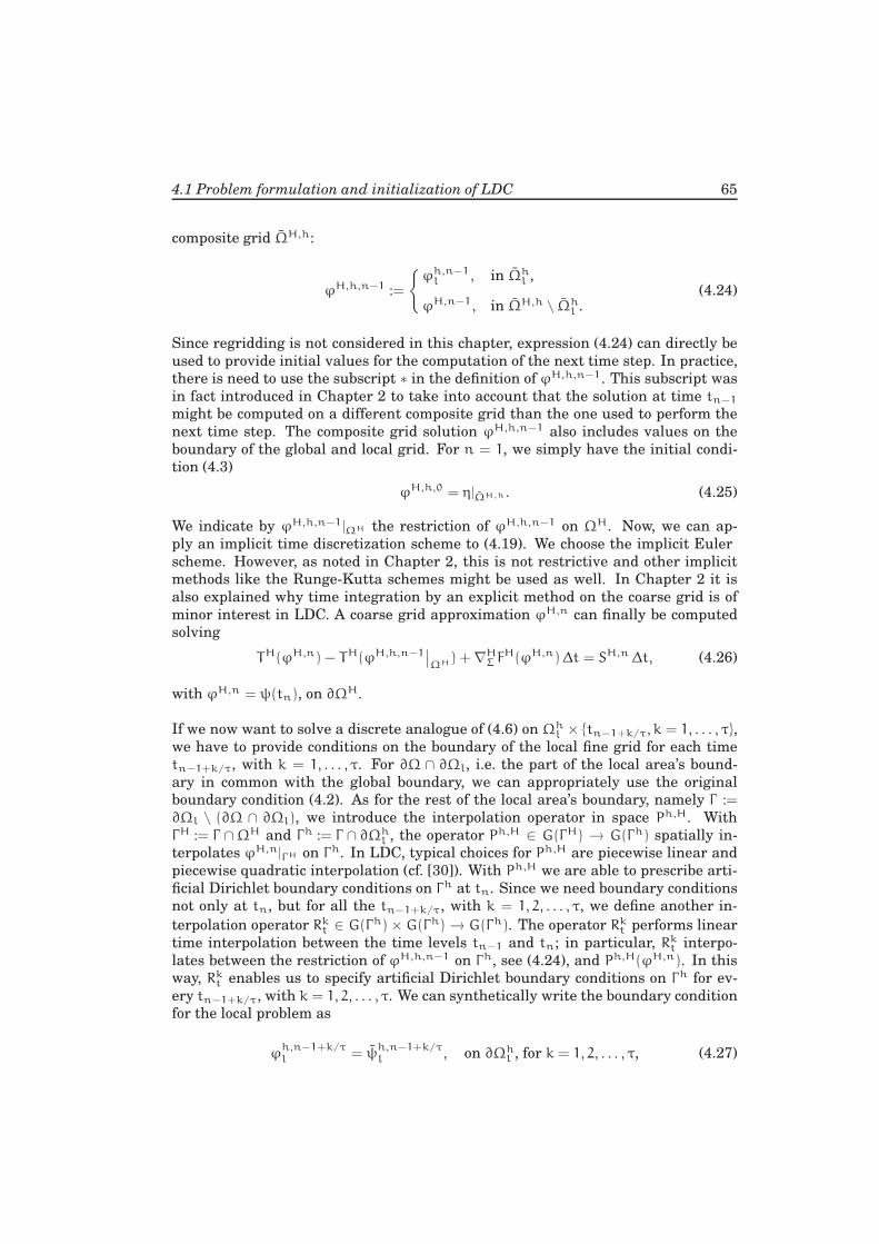
4.1 Problem formulation and initialization of LDC 65
composite grid ΩH,h:
ϕH,h,n−1 :=
ϕh,n−1
l , in Ωhl ,
ϕH,n−1, in ΩH,h \ Ωhl .
(4.24)
Since regridding is not considered in this chapter, expression (4.24) can directly be
used to provide initial values for the computation of the next time step. In practice,
there is need to use the subscript ∗ in the definition of ϕH,h,n−1. This subscript was
in fact introduced in Chapter 2 to take into account that the solution at time tn−1
might be computed on a different composite grid than the one used to perform the
next time step. The composite grid solution ϕH,h,n−1 also includes values on the
boundary of the global and local grid. For n = 1, we simply have the initial condi-
tion (4.3)
ϕH,h,0 = η|ΩH,h . (4.25)
We indicate by ϕH,h,n−1|ΩH the restriction of ϕH,h,n−1 on ΩH. Now, we can ap-
ply an implicit time discretization scheme to (4.19). We choose the implicit Euler
scheme. However, as noted in Chapter 2, this is not restrictive and other implicit
methods like the Runge-Kutta schemes might be used as well. In Chapter 2 it is
also explained why time integration by an explicit method on the coarse grid is of
minor interest in LDC. A coarse grid approximation ϕH,n can finally be computed
solving
TH(ϕH,n) − TH(ϕH,h,n−1∣
∣
ΩH) + ∇HΣ F
H(ϕH,n)∆t = SH,n ∆t, (4.26)
with ϕH,n = ψ(tn), on ∂ΩH.
If we now want to solve a discrete analogue of (4.6) on Ωhl × tn−1+k/τ, k = 1, . . . , τ,
we have to provide conditions on the boundary of the local fine grid for each time
tn−1+k/τ, with k = 1, . . . , τ. For ∂Ω ∩ ∂Ωl, i.e. the part of the local area’s bound-
ary in common with the global boundary, we can appropriately use the original
boundary condition (4.2). As for the rest of the local area’s boundary, namely Γ :=
∂Ωl \ (∂Ω ∩ ∂Ωl), we introduce the interpolation operator in space Ph,H. With
ΓH := Γ ∩ΩH and Γh := Γ ∩ ∂Ωhl , the operator Ph,H ∈ G(ΓH) → G(Γh) spatially in-
terpolates ϕH,n|ΓH on Γh. In LDC, typical choices for Ph,H are piecewise linear and
piecewise quadratic interpolation (cf. [30]). With Ph,H we are able to prescribe arti-
ficial Dirichlet boundary conditions on Γh at tn. Since we need boundary conditions
not only at tn, but for all the tn−1+k/τ, with k = 1, 2, . . . , τ, we define another in-
terpolation operator Rkt ∈ G(Γh) × G(Γh)→ G(Γh). The operator Rk
t performs linear
time interpolation between the time levels tn−1 and tn; in particular, Rkt interpo-
lates between the restriction of ϕH,h,n−1 on Γh, see (4.24), and Ph,H(ϕH,n). In this
way, Rkt enables us to specify artificial Dirichlet boundary conditions on Γh for ev-
ery tn−1+k/τ, with k = 1, 2, . . . , τ. We can synthetically write the boundary condition
for the local problem as
ϕh,n−1+k/τ
l = ψh,n−1+k/τ
l , on ∂Ωhl , for k = 1, 2, . . . , τ, (4.27)
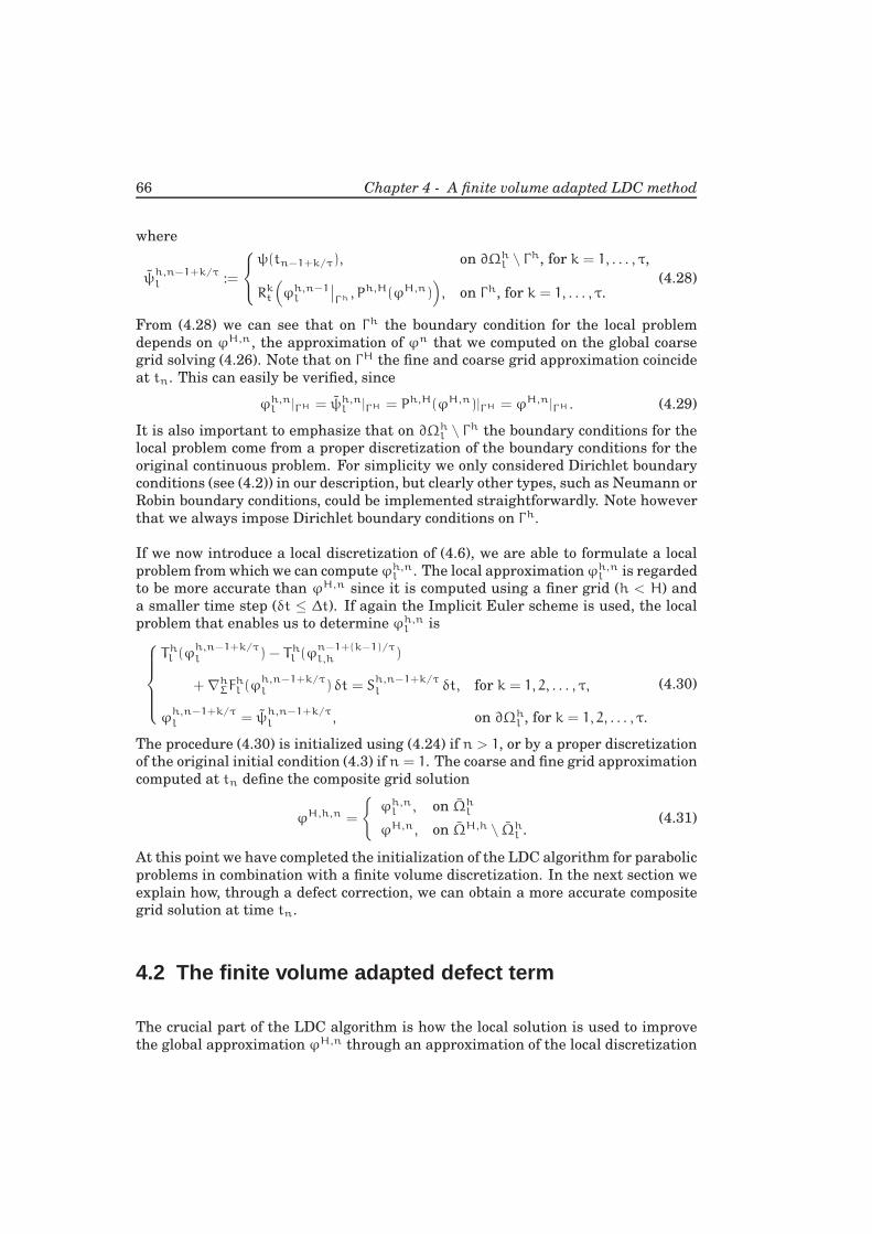
66 Chapter 4 - A finite volume adapted LDC method
where
ψh,n−1+k/τ
l :=
ψ(tn−1+k/τ), on ∂Ωhl \ Γh, for k = 1, . . . , τ,
Rkt
(
ϕh,n−1l
∣
∣
Γh , Ph,H(ϕH,n)
)
, on Γh, for k = 1, . . . , τ.(4.28)
From (4.28) we can see that on Γh the boundary condition for the local problem
depends on ϕH,n, the approximation of ϕn that we computed on the global coarse
grid solving (4.26). Note that on ΓH the fine and coarse grid approximation coincide
at tn. This can easily be verified, since
ϕh,nl |ΓH = ψh,n
l |ΓH = Ph,H(ϕH,n)|ΓH = ϕH,n|ΓH . (4.29)
It is also important to emphasize that on ∂Ωhl \ Γh the boundary conditions for the
local problem come from a proper discretization of the boundary conditions for the
original continuous problem. For simplicity we only considered Dirichlet boundary
conditions (see (4.2)) in our description, but clearly other types, such as Neumann or
Robin boundary conditions, could be implemented straightforwardly. Note however
that we always impose Dirichlet boundary conditions on Γh.
If we now introduce a local discretization of (4.6), we are able to formulate a local
problem from which we can computeϕh,nl . The local approximationϕh,n
l is regarded
to be more accurate than ϕH,n since it is computed using a finer grid (h < H) and
a smaller time step (δt ≤ ∆t). If again the Implicit Euler scheme is used, the local
problem that enables us to determine ϕh,nl is
Thl (ϕ
h,n−1+k/τ
l ) − Thl (ϕ
n−1+(k−1)/τ
l,h )
+ ∇hΣF
hl (ϕ
h,n−1+k/τ
l ) δt = Sh,n−1+k/τ
l δt, for k = 1, 2, . . . , τ,
ϕh,n−1+k/τ
l = ψh,n−1+k/τ
l , on ∂Ωhl , for k = 1, 2, . . . , τ.
(4.30)
The procedure (4.30) is initialized using (4.24) if n > 1, or by a proper discretization
of the original initial condition (4.3) if n = 1. The coarse and fine grid approximation
computed at tn define the composite grid solution
ϕH,h,n =
ϕh,n
l , on Ωhl
ϕH,n, on ΩH,h \ Ωhl .
(4.31)
At this point we have completed the initialization of the LDC algorithm for parabolic
problems in combination with a finite volume discretization. In the next section we
explain how, through a defect correction, we can obtain a more accurate composite
grid solution at time tn.
4.2 The finite volume adapted defect term
The crucial part of the LDC algorithm is how the local solution is used to improve
the global approximation ϕH,n through an approximation of the local discretization
4.2 The finite volume adapted defect term 67
error or defect. In particular, like it is done in [6] for elliptic problems, we are
interested in expressing the defect in such a way that the resulting composite grid
discretization satisfies a discrete conservation law. The defect dH,n ∈ G(ΩH) is
defined as
dH,n := TH(ϕn|ΩH) − TH(ϕn−1 |ΩH) + ∇HΣ F
H(ϕn|ΩH)∆t− SH,n ∆t. (4.32)
In (4.32) we have plugged the exact analytical solution ϕ into the coarse grid dis-
cretization scheme (4.26). We consider now the continuous equation (4.6), which is
valid for all volumes V ⊂ Ω and thus for any control volume Vi,j ⊂ Ω too. If we
apply time integration between tn−1 and tn, we obtain
∫
Vi,j
ϕn dΩ−
∫
Vi,j
ϕn−1 dΩ+
∫tn
tn−1
∫
∂Vi,j
f · n dγ dt
=
∫tn
tn−1
∫
Vi,j
sdΩdt, for i = 1, 2, . . . , Nx − 1, j = 1, 2, . . . , Ny − 1, (4.33)
or
T(ϕn) − T(ϕn−1) +
∫tn
tn−1
∇HΣ F(ϕ) dt =
∫tn
tn−1
Sdt. (4.34)
Combination of (4.34) and (4.32) yields
dH,n =(
TH(ϕn|ΩH) − T(ϕn))
−(
TH(ϕn−1|ΩH) − T(ϕn−1))
+ ∇HΣ
(
FH(ϕn|ΩH)∆t −
∫tn
tn−1
F(ϕ) dt
)
−
(
SH,n ∆t−
∫tn
tn−1
Sdt
)
,
(4.35)
which is the definition of defect that we will use in practice. If we would know the
values of dH,n, we could use them to compute a more accurate (both in space and
time) approximation of ϕn on the global grid. This could be done by adding dH,n
on the right hand side of (4.26). However, since we do not know the exact solution
of our partial differential equation, we cannot compute the values of dH,n. What
we can do, though, is to use the local solution ϕh,nl to get an estimate of dH,n. We
introduce
dH,nT := TH(ϕn|ΩH) − T(ϕn), (4.36)
dH,nF := FH(ϕn|ΩH)∆t−
∫ tn
tn−1
F(ϕ) dt, (4.37)
dH,nS := SH,n ∆t −
∫tn
tn−1
Sdt, (4.38)
so that, cf. (4.35),
dH,n = dH,nT − dH,n−1
T + ∇HΣd
H,nF − dH,n
S . (4.39)
In the following section we will approximate each of the terms that appear on the
right hand side of (4.39).
68 Chapter 4 - A finite volume adapted LDC method
4.2.1 Approximation of the defect
We start by considering dH,nT . After solving the global and the local problem, the
following approximations are available for an arbitrary Ti,j(ϕn):
1) the coarse grid approximation THi,j(ϕ
H,n);
2) a coarse grid approximation that based on the composite grid solution (4.31),
i.e. THi,j(ϕ
H,h,n|ΩH);
3) a sum of fine grid approximations
T suml,i,j(ϕ
h,nl ) :=
(σx−1)/2∑
p=−(σx−1)/2
(σy−1)/2∑
q=−(σy−1)/2
Thl,i+p/σx,j+q/σy
(ϕh,nl ). (4.40)
In T suml,i,j the subscript l reminds us that this third approximation is local and it
exists only for (xi, yj) ∈ Ωl, i.e. for the coarse grid points lying in the area of
refinement.
The approximations above are considered to be listed in order of increasing accuracy.
The second approximation is more accurate than the first one because in the area
of refinement it exploits the values computed on the fine grid with a time step δt ≤∆t. The approximation number three can be considered more accurate than the
second one because it computes spatial integrals using the fine grid discretization.
We introduce ΩHl := ΩH ∩Ωh
l and we use the best available information to define
Tbest(ϕH,h,n) ∈ G(ΩH) as
Tbest(ϕH,h,n) :=
T sum
l (ϕh,nl ), on ΩH
l ,
TH(ϕH,h,n), on ΩH \ΩHl .
(4.41)
Definition (4.41) is used to introduce the following approximation for dH,nT :
dH,nT = TH(ϕn|ΩH) − T(ϕn) ≈ TH(ϕH,h,n|ΩH) − Tbest(ϕH,h,n) =: dH,n
T . (4.42)
Combining (4.41) and (4.42) it is easy to show that
dH,nT = 0, on ΩH \ΩH
l . (4.43)
We consider now the flux discretization error dH,nF , see (4.37), and in particular
Fni+1/2,j :=
∫tn
tn−1
Fi+1/2,j(ϕ) dt, (4.44)
where Fi+1/2,j is an arbitrary horizontal flux. In the expression of Fni+1/2,j both
space (cf. (4.16)) and time integrals appear; these can be approximated in different
ways, using the coarse or the fine grid size, the ∆t or the δt time discretization.
Below we list the possible approximations for Fni+1/2,j
:
4.2 The finite volume adapted defect term 69
1) an H-∆t approximation, i.e. an approximation based on the H space discretiza-
tion and on the ∆t time discretization:
Fni+1/2,j ≈
∫tn
tn−1
FHi+1/2,j
(
ϕH(t))
dt ≈ FHi+1/2,j(ϕ
H,n)∆t; (4.45)
2) an (H,h)-∆t approximation based on the composite grid solution (4.31):
Fni+1/2,j ≈
∫tn
tn−1
FHi+1/2,j
(
ϕH,h(t)|ΩH
)
dt ≈ FHi+1/2,j(ϕ
H,h,n|ΩH)∆t; (4.46)
3) a local h-∆t approximation based on the sum of fine grid fluxes. We introduce
Fsuml,i+1/2,j(ϕ
hl (t)) :=
(σy−1)/2∑
q=−(σy−1)/2
Fhl,i+1/2,j+q/σy
(ϕhl (t)), (4.47)
and we write
Fni+1/2,j ≈
∫tn
tn−1
Fsuml,i+1/2,j
(
ϕhl (t)
)
dt ≈ Fsuml,i+1/2,j(ϕ
h,nl )∆t; (4.48)
4) a local h-δt approximation based on the δt time discretization:
Fni+1/2,j ≈
∫tn
tn−1
Fsuml,i+1/2,j(ϕ
hl (t)) dt
=
τ∑
k=1
∫tn−1+k/τ
tn−1+(k−1)/τ
Fsuml,i+1/2,j(ϕ
hl (t)) dt
≈τ∑
k=1
Fsuml,i+1/2,j(ϕ
h,n−1+k/τ
l ) δt.
(4.49)
As before the various approximations are listed in order of increasing accuracy. The
third and the fourth approximation can only be expressed for points (xi+1/2, yj) ∈Ωl. Analogous approximations are available for the other flux terms, i.e Fi−1/2,j,
Fi,j+1/2, Fi,j−1/2. We can therefore define Fbest ∈ G(VH) and Fbest ∈ G(VH) as
Fbest(ϕH,h,n) := Fbest(ϕH,h,n)∆t :=
τ∑
k=1
Fsuml (ϕ
h,n−1+k/τ
l ) δt, on VH ∩Ωl,
FH(ϕH,h,n|ΩH)∆t, elsewhere.
We can now approximate dH,nF as
dH,nF = FH(ϕn|ΩH)∆t−
∫tn
tn−1
F(ϕ) dt
≈ FH(ϕH,h,n|ΩH)∆t− Fbest(ϕH,h,n)∆t =: dH,nF .
(4.50)
70 Chapter 4 - A finite volume adapted LDC method
Combination of (4.50) with the definition of Fbest(ϕH,h,n) yields
dH,nF = 0, on VH \ (VH ∩Ωl). (4.51)
Similar considerations hold for an arbitrary source term
Sni,j :=
∫ tn
tn−1
Si,j(t) dt, (4.52)
which can be approximated through:
1) an H-∆t approximation
Sni,j ≈
∫tn
tn−1
SHi,j(t) dt ≈ SH,n
i,j ∆t. (4.53)
This approximation is global and holds for all 1 ≤ i ≤ Nx−1 and 1 ≤ j ≤ Ny−1;
2) a local h-∆t approximation based on a sum of fine grid approximations and on
a ∆t time integration. We introduce
Ssuml,i,j(t) :=
(σx−1)/2∑
p=−(σx−1)/2
(σy−1)/2∑
q=−(σy−1)/2
Shl,i+p/σx,j+q/σy
(t), (4.54)
and we write
Sni,j ≈
∫tn
tn−1
Ssuml,i,j(t) dt ≈ Ssum,n
l,i,j ∆t. (4.55)
The approximation (4.55) holds for (xi, yj) ∈ ΩHl ;
3) a local h-δt approximation
Sni,j ≈
∫ tn
tn−1
Ssuml,i,j(t) dt
=
τ∑
k=1
∫tn−1+k/τ
tn−1+(k−1)/τ
Ssuml,i,j(t) dt ≈
τ∑
k=1
Ssum,n−1+k/τ
l,i,j δt,
(4.56)
defined for points (xi, yj) ∈ ΩHl .
Gathering the best available information, we define Sbest,n ∈ G(ΩH) and Sbest,n ∈G(ΩH) as
Sbest,n := Sbest,n ∆t :=
τ∑
k=1
Ssum,n−1+k/τ
l,i,j δt, on ΩHl ,
SH,n ∆t, on ΩH \ΩHl .
(4.57)
4.2 The finite volume adapted defect term 71
It is now possible to provide an approximation for dH,nS :
dH,nS := SH,n ∆t−
∫tn
tn−1
Sdt ≈ SH,n ∆t− Sbest,n ∆t =: dH,nS . (4.58)
We note that combination of (4.57) and (4.58) yields
dH,nS = 0, on ΩH \ΩH
l . (4.59)
4.2.2 The finite volume adapted LDC algorithm
In the previous section we have found an approximation for all the terms that ap-
pear on the right hand side of (4.39). where dH,n ∈ G(ΩH) is defined by (cf. (4.42),
(4.50) and (4.58))
dH,n := dH,nT − dH,n−1
T + ∇HΣ d
H,nF − dH,n
S
=(
TH(ϕH,h,n|ΩH) − Tbest(ϕH,h,n))
−(
TH(ϕH,h,n−1 |ΩH) − Tbest(ϕH,h,n−1))
+ ∆t∇HΣ
(
FH(ϕH,h,n|ΩH) − Fbest(ϕH,h,n))
− ∆t(
SH,n − Sbest,n)
. (4.60)
The approximation dH,n clearly depends on the solution computed on the fine grid
in the time interval [tn−1, tn]. We can finally compute a more accurate global ap-
proximation of ϕn solving the modified coarse grid problem
TH(ϕH,n1 ) − TH(ϕH,h,n−1
∣
∣
ΩH) + ∇HΣ F
H(ϕH,n1 )∆t = SH,n ∆t+ dH,n, (4.61)
with ϕH,n1 = ψ(tn), on ∂ΩH. In (4.61) we called the new approximation ϕH,n
1 , where
the new subscript is used to distinguish the new approximation from the previous
one ϕH,n, from now on referred as ϕH,n0 . Once ϕH,n
1 is computed, we are able to
define new boundary conditions, see (4.27), for a new local problem on Ωhl and this
triggers an iterative procedure which is formalized in Algorithm 4.1. As for the
global grid solution, in Algorithm 4.1 an extra subscript is added to number the
different approximations computed locally; the same is done for the defect term.
Algorithm 4.1 (Finite volume adapted LDC algorithm)
FOR LOOP, n = 1, 2, . . . , Nt
INITIALIZATION
• Compute a global approximation ϕH,n0 ∈ G(ΩH) solving
problem (4.26), with ϕH,n0 = ψ(tn) on ∂ΩH.
• Compute a local approximation ϕh,nl,0 ∈ G(Ωh
l ) solving thelocal problem (4.30).
• Define ϕH,h,n0 ∈ G(ΩH,h) as in (4.31).
72 Chapter 4 - A finite volume adapted LDC method
ITERATION, w = 1, 2, . . .
• Compute dH,nw−1 ∈ G(ΩH), an approximation of the local dis-
cretization error dnH ∈ G(ΩH), through
dH,nw−1 =
(
TH(ϕH,h,nw−1 |ΩH) − Tbest(ϕn
H,h,w−1))
−(
TH(ϕH,h,n−1|ΩH) − Tbest(ϕH,h,n−1))
+ ∆t∇HΣ
(
FH(ϕH,h,nw−1 |ΩH) − Fbest(ϕn
H,h,w−1))
− ∆t(
SH,n − Sbest,n)
. (4.62)
• Compute a more accurate global coarse grid approximationϕH,n
w ∈ G(ΩH) solving the modified problem
TH(ϕH,nw ) − TH(ϕH,h,n−1
∣
∣
ΩH)
+∇HΣ F
H(ϕH,nw )∆t = SH,n ∆t+ dH,n
w−1,
ϕH,nw = ψ(tn), on ∂ΩH.
(4.63)
• Use ϕH,nw to update the boundary condition ψh
l,w on ∂Ωhl .
• Solve the following local problem with updated boundary
conditions
Thl (ϕ
h,n−1+k/τ
l,w ) − Thl (ϕ
h,n−1+(k−1)/τ
l,w )
+∇hΣF
hl (ϕ
h,n−1+k/τ
l,w ) δt = Sh,n−1+k/τ
l δt,
ϕh,n−1+k/τ
l,w = ψh,n−1+k/τ
l,w , on ∂Ωhl ,
(4.64)
for k = 1, 2, . . . , τ.
• Define the composite grid approximation
ϕH,h,nw =
ϕh,n
l,w , on Ωhl
ϕH,nw , on ΩH \ΩH
l .(4.65)
END ITERATION ON w
• Call ϕh,nl and ϕH,n the latest solutions found on the local
and global grid respectively (remove the last subscript); thesolution on the composite grid at time tn is:
ϕH,h,n :=
ϕh,n
l , in Ωhl ,
ϕH,n, in ΩH,h \ Ωhl .
(4.66)
END FOR
4.2 The finite volume adapted defect term 73
This is the LDC algorithm for time-dependent problems as presented in Chapter 2,
but now adapted to a setting with a finite volume discretization. Like done in [6] for
stationary cases, the expression of the defect term dH,nw−1 is such that the resulting
composite grid discretization is still conservative. This property of the finite volume
adapted LDC method is discussed in Section 4.3. Before that, Section 4.2.3, we give
a practical way to compute the defect term (4.62).
4.2.3 Practical considerations on the defect term
In practice the defect term dH,nw−1 is not computed through a straightforward applica-
tion of (4.62). That would in fact be quite onerous, since it would require to sum fine
grid values at all the points Ωhl and for all the times tn−1+k/τ, with k = 1, 2, . . . , τ.
In the perspective of simplifying the computation of dH,nw−1, in Lemma 4.2 we state
a local conservation law that holds just for the points (xi, yj) ∈ ΩHl . This is ob-
tained summing the fine grid balance of each fine grid control volume at each time
tn−1+k/τ, with k = 1, 2, . . . , τ.
Lemma 4.2
The fine grid approximation is such that
T suml,i,j(ϕ
h,nl,w ) − T sum
l,i,j(ϕH,h,n−1|Ωh
l) +
(
∇HΣ
τ∑
k=1
Fsuml (ϕ
h,n−1+k/τ
l,w )
)
i,j
δt
=
τ∑
k=1
Ssum,n−1+k/τ
l,i,j δt for (xi, yj) ∈ ΩHl . (4.67)
Proof. We consider the fine grid balance in (4.64) and we sum it for all the σxσy
fine grid control volumes that partition a coarse grid control volume Vi,j ⊂ Ωl. We
obtain
(σx−1)/2∑
p=−(σx−1)/2
(σy−1)/2∑
q=−(σy−1)/2
(
Thl,i+p,j+q(ϕ
h,n−1+k/τ
l,w ) − Thl,i+p,j+q(ϕ
h,n−1+k/τ
l,w )
)
+
(σx−1)/2∑
p=−(σx−1)/2
(σy−1)/2∑
q=−(σx−1)/2
(
∇hΣF
hl (ϕ
h,n−1+k/τ
l,w ) δt
)
i+p,j+q
=
=
(σx−1)/2∑
p=−(σx−1)/2
(σy−1)/2∑
q=−(σy−1)/2
(
Sh,n−1+k/τ
l,i+p,j+q δt
)
for (xi, yj) ∈ ΩHl , k = 1, 2, . . . , τ.
(4.68)
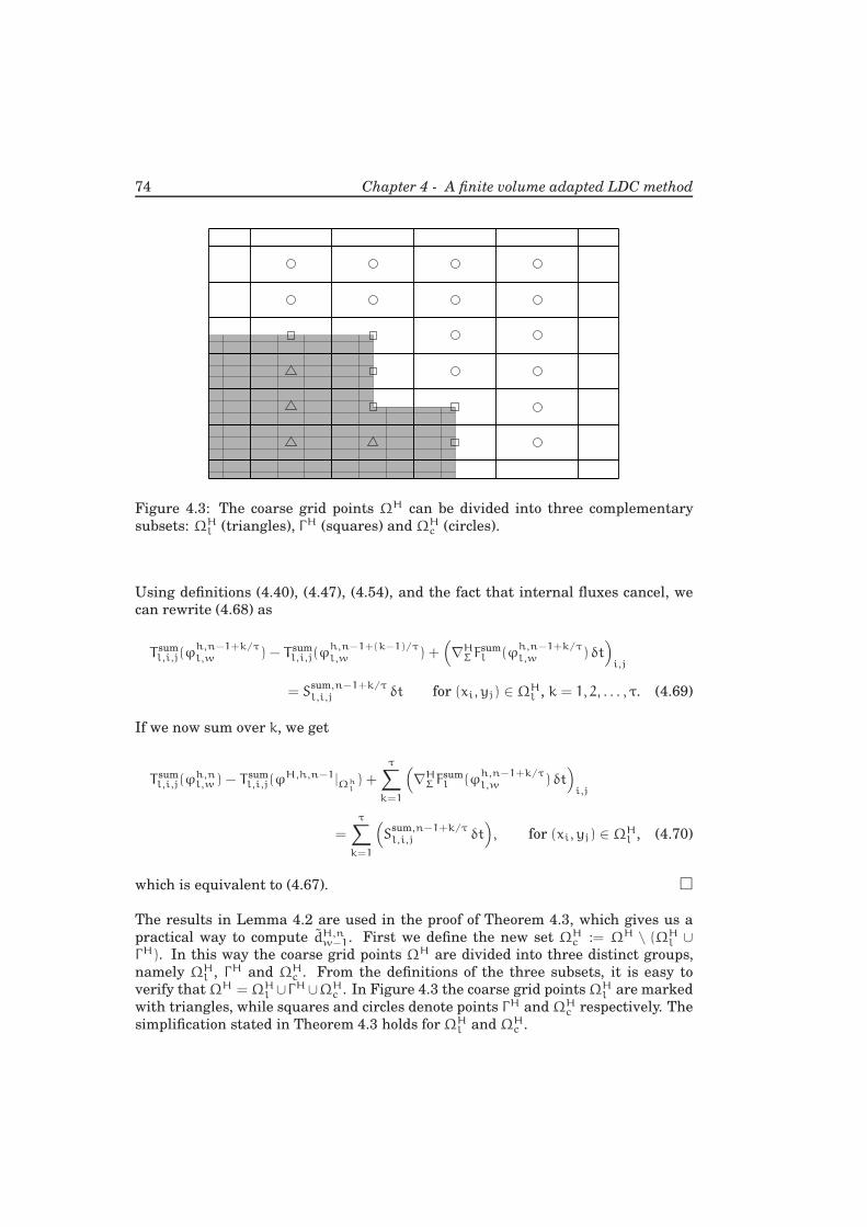
74 Chapter 4 - A finite volume adapted LDC method
Figure 4.3: The coarse grid points ΩH can be divided into three complementary
subsets: ΩHl (triangles), ΓH (squares) and ΩH
c (circles).
Using definitions (4.40), (4.47), (4.54), and the fact that internal fluxes cancel, we
can rewrite (4.68) as
T suml,i,j(ϕ
h,n−1+k/τ
l,w ) − T suml,i,j(ϕ
h,n−1+(k−1)/τ
l,w ) +(
∇HΣ F
suml (ϕ
h,n−1+k/τ
l,w ) δt)
i,j
= Ssum,n−1+k/τ
l,i,j δt for (xi, yj) ∈ ΩHl , k = 1, 2, . . . , τ. (4.69)
If we now sum over k, we get
T suml,i,j(ϕ
h,nl,w ) − T sum
l,i,j(ϕH,h,n−1|Ωh
l) +
τ∑
k=1
(
∇HΣ F
suml (ϕ
h,n−1+k/τ
l,w ) δt)
i,j
=
τ∑
k=1
(
Ssum,n−1+k/τ
l,i,j δt)
, for (xi, yj) ∈ ΩHl , (4.70)
which is equivalent to (4.67).
The results in Lemma 4.2 are used in the proof of Theorem 4.3, which gives us a
practical way to compute dH,nw−1. First we define the new set ΩH
c := ΩH \ (ΩHl ∪
ΓH). In this way the coarse grid points ΩH are divided into three distinct groups,
namely ΩHl , ΓH and ΩH
c . From the definitions of the three subsets, it is easy to
verify thatΩH = ΩHl ∪ΓH∪ΩH
c . In Figure 4.3 the coarse grid pointsΩHl are marked
with triangles, while squares and circles denote points ΓH andΩHc respectively. The
simplification stated in Theorem 4.3 holds for ΩHl and ΩH
c .
4.2 The finite volume adapted defect term 75
Theorem 4.3
The defect term dH,nw−1 ∈ G(ΩH) can be written as
(dH,nw−1)i,j =
THi,j(ϕ
H,h,nw−1 |ΩH) − TH
i,j(ϕH,h,n−1|ΩH)
+(
∇HΣ F
H(ϕH,h,nw−1 |ΩH)
)
i,j∆t
− SH,ni,j ∆t, for (xi, yj) ∈ ΩH
l ,
0 for (xi, yj) ∈ ΩHc .
(4.71)
Proof. Consider a point (xi, yj) ∈ ΩHl . We have
(dH,nw−1)i,j
(4.62)=(
THi,j(ϕ
H,h,nw−1 |ΩH) − T sum
l,i,j(ϕh,nl,w−1)
)
−(
THi,j(ϕ
H,h,n−1w−1 |ΩH) − T sum
l,i,j(ϕH,h,n−1w−1 |Ωh
l))
+
(
∇HΣ
(
FH(ϕH,h,nw−1 |ΩH)∆t −
τ∑
k=1
Fsuml (ϕ
H,h,n−1+k/τ
w−1 ) δt)
)
i,j
−(
SH,ni,j ∆t−
τ∑
k=1
Ssum,n−1+k/τ
l,i,j δt)
(4.67)= TH
i,j(ϕH,h,nw−1 |ΩH) − TH
i,j(ϕH,h,n−1|ΩH)
+(
∇HΣ F
H(ϕH,h,nw−1 |ΩH)
)
i,j∆t− SH,n
i,j ∆t.
(4.72)
This proves the first part of (4.71). The second part can be proved combining (4.62)
for a point (xi, yj) ∈ ΩHc with (4.43), (4.51) and (4.59).
Theorem 4.3 gives us formulas to compute the finite volume adapted defect term on
ΩHl ∪ ΩH
c . Therefore we need the original definition (4.62) for points ΓH only. We
note however that even on ΓH things can be simplified significantly. Combination
of (4.62) for a point (xi, yj) ∈ ΓH with formulas (4.43) and (4.59) yields in fact
dH,nw−1 = ∆t∇H
Σ
(
FH(ϕH,h,nw−1 |ΩH) − Fbest(ϕn
H,h,w−1))
, on ΓH. (4.73)
The only term on the right hand side of (4.62) that we explicitly have to compute for
a point (xi, yj) ∈ ΓH is thus the sum of the fine grid fluxes.
Note that Theorem 4.3 not only gives us a practical way to compute the finite volume
adapted defect term (4.62), but it also establishes the connection between the LDC
method with the finite volume adapted defect term introduced here and the LDC
method with the standard defect term presented in Chapter 2. OnΩHl the standard
defect term is computed plugging the fine grid solution at time tn into the coarse grid
discretization scheme. This is what happens in the first part of (4.71) too. Elsewhere
76 Chapter 4 - A finite volume adapted LDC method
the standard defect is zero. This is not true for the finite volume adapted defect
term, which is zero on ΩHc only. On ΓH it is not zero and the balance of integrated
fluxes guaranteed by (4.73) is such that the finite volume adapted LDC method
produces a solution that satisfies a discrete conservation law on the composite grid.
This is explained in Section 4.3.
4.3 Conservation properties of LDC
We discuss a few properties of the LDC algorithm described in Sections 4.1 and 4.2.
The time-dependent LDC technique is an iterative procedure that implicitly gives a
discretization of the convection-diffusion problem on a composite grid at the discrete
time levels tn = n∆t, with n = 1, 2, . . . , Nt. Throughout this section, we will assume
that at each time tn the LDC iteration converges. A sufficient condition for the
iterative procedure to be convergent is that for every n = 1, 2, . . . , Nt the vector
norm
‖ϕH,nw −ϕH,n
w−1‖→ 0, (w→∞). (4.74)
Condition (4.74) implies that
‖ψh,n−1+(k−1)/τ
l,w − ψh,n−1+(k−1)/τ
l,w−1 ‖→ 0, (w→∞), ∀k = 1, 2, . . . , τ, (4.75)
and therefore
‖ϕh,nl,w −ϕh,n
l,w−1‖→ 0, (w→∞). (4.76)
When the LDC iteration at tn has converged, the subscript w is removed, and the
converged global and local solution are called ϕH,n ∈ G(ΩH) and ϕh,nl ∈ G(Ωh
l )
respectively. They define a composite grid approximation ϕH,h,n ∈ G(ΩH,h) as
in (4.66). In Lemma 4.4 we show that the converged coarse grid solution ϕH,n and
the converged fine grid solution ϕh,nl coincide in ΩH
l for n > 1. Note that this prop-
erty is automatically verified for n = 0 (initial condition).
Lemma 4.4
Assume that the local coarse grid stationary homogeneous system
THi,j(ν) +
(
∇HΣ F
H(ν))
i,j= 0, for (xi, yj) ∈ ΩH
l ,
ν = 0, for (xi, yj) ∈ ΓH,
(4.77)
has only the zero solution in G(ΩHl ∪ΓH). Then the limit solution (ϕH,n, ϕh,n
l ) of theLDC iteration at time tn (n > 1) satisfies
ϕH,n = ϕh,nl , on ΩH
l . (4.78)
4.3 Conservation properties of LDC 77
Proof. From (4.63) and (4.71), we obtain
THi,j(ϕ
H,n) +(
∇HΣ F
H(ϕH,n))
i,j
= THi,j(ϕ
H,h,n|ΩH) +(
∇HΣ F
H(ϕH,h,n|ΩH))
i,jfor (xi, yj) ∈ ΩH
l . (4.79)
or
THi,j(ϕ
H,n−ϕH,h,n|ΩH)+(
∇HΣ F
H(ϕH,n−ϕH,h,n|ΩH))
i,j= 0 for (xi, yj) ∈ ΩH
l . (4.80)
Moreover, from (4.29) and (4.66), we can deduce thatϕH,n|ΓH−ϕH,h,n|ΓH = 0. Hence,
ν = ϕH,n − ϕH,h,n|ΩH ∈ G(ΩHl ∪ ΓH) satisfies system (4.77). From the assumption,
ν is null on ΩHl ∪ ΓH, which is equivalent to (4.78) because ϕH,h,n ≡ ϕh,n
l on ΩHl
(see (4.66)).
The results of Lemma 4.4 will be used in the proof of Theorem 4.5, which gives
the discrete conservation law that is satisfied by the converged composite grid solu-
tion ϕH,h,n. Before that, we consider for a while what happens when problem (4.6)
is discretized on a global grid ΩH by the finite volume method. Again, for simplic-
ity, we consider the implicit Euler scheme for time discretization. The following
conservation law
THi,j(ϕ
H,n) − THi,j(ϕ
H,n−1) +(
∇HΣ F
H(ϕH,n))
i,j∆t = SH,n
i,j ∆t (4.81)
holds for any control volume Vi,j ⊂ ΩH. Formula (4.81) is a discrete equivalent of
the continuous conservation law (4.6). Summation of the discrete conservation laws
that hold for individual control volumes Vi,j leads to a conservation law on the union
of these control volumes. This is because fluxes over internal faces cancel: in a time
step ∆t, the influx into Vi,j ⊂ ΩH out a neighboring control volume Vl,m ⊂ ΩH is
balanced by the outflux from Vi,j to Vl,m in the same time step. Theorem 4.5 states
that this property is also verified for the limit of the LDC iteration ϕH,h,n, which is
computed on a composite grid using two different time integration steps ∆t and δt.
This is the generalization to time-dependent problems of the conservation property
presented in [6] for the LDC method in stationary cases.
Theorem 4.5
Under the assumption of Lemma 4.4, the composite grid solution satisfies the fol-lowing system of discrete conservation laws:
Tbest(ϕH,h,n) − Tbest(ϕH,h,n−1) + ∇HΣ F
best(ϕH,h,n)∆t = Sbest,n∆t. (4.82)
Proof. Combination of (4.63) and (4.62) yields
TH(ϕH,n) + ∇HΣ F
H(ϕH,n)∆t = TH(ϕH,h,n|ΩH) − Tbest(ϕH,h,n) + Tbest(ϕH,h,n−1)
+ ∇HΣ
(
FH(ϕH,h,n)|ΩH − Fbest(ϕH,h,n))
∆t+ Sbest,n∆t. (4.83)
78 Chapter 4 - A finite volume adapted LDC method
Using Lemma 4.4, we have
TH(ϕH,n) = TH(ϕH,h,n|ΩH), FH(ϕH,n) = FH(ϕH,h,n|ΩH). (4.84)
Substitution of (4.84) into (4.83) gives (4.82).
We note that, for (xi, yj) ∈ ΩHl , the conservation laws (4.82) reduce to
T suml,i,j(ϕ
h,nl ) − T sum
l,i,j(ϕh,n−1l )
+
(
∇HΣ
τ∑
k=1
Fsuml (ϕ
h,n−1+k/τ
l ) δt
)
i,j
=
τ∑
k=1
Ssum,n−1+k/τ
l,i,j δt. (4.85)
This is the same relation we deduced in Lemma 4.2 summing the conservation laws
that hold for each of the σxσy fine grid control volume that partition Vi,j ⊂ Ωl for
all the times tn−1+k/τ, with k = 1, 2, . . . , τ. For (xi, yj) ∈ ΩHc , balance (4.82) becomes
THi,j(ϕ
H,n) − THi,j(ϕ
H,n−1) +(
∇HΣ F
H(ϕH,n))
i,j∆t = SH,n
i,j ∆t, (4.86)
which is clearly the set of conservation laws that correspond to the coarse grid dis-
cretization with time step ∆t. For points (xi, yj) ∈ ΓH, Theorem 4.5 guarantees that,
in a time step ∆t, the discrete influx into Vi,j out of a neighboring volume Vl,m,
with (xl, ym) ∈ Ωl, matches the total discrete outflux from Vl,m to Vi,j in the same
time step ∆t. The latter is the sum of all the fine grid fluxes at all the intermediate
times tn−1+k/τ, with k = 1, 2, . . . , τ. In practice, when we sum discrete conserva-
tion laws that hold on individual control volumes Vi,j, the finite volume adapted
LDC method is such that internal fluxes cancel like it happens for the finite volume
discretization on a single grid. We note that (4.82) holds for the fully converged com-
posite grid solution ϕH,h,n. However, as it happens for the standard LDC method
for parabolic problems, the convergence of the finite volume adapted LDC algorithm
is generally very fast and only very few iterations suffice.
When presenting the finite volume adapted LDC method, we considered a vertex-
centered discretization for both coarse and fine grid, but we noted that other ap-
proaches, like a cell-centered discretization, could be used as well. Figure 4.4 shows
an example of composite grid where the global coarse grid is treated with a cell-
centered approach, i.e. the domain boundary coincides with control volume bound-
aries. As a consequence of this choice, the fine grid is treated like in the cell-centered
method along ∂Ωl ∩ Ω, i.e. the part of the local region’s boundary which is in com-
mon with the physical boundary, and like in the vertex-centered method along the
interface Γ . This approach is followed in the numerical experiments we present in
Section 4.4, Chapter 5 and Chapter 6.
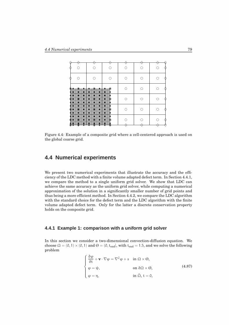
4.4 Numerical experiments 79
Figure 4.4: Example of a composite grid where a cell-centered approach is used on
the global coarse grid.
4.4 Numerical experiments
We present two numerical experiments that illustrate the accuracy and the effi-
ciency of the LDC method with a finite volume adapted defect term. In Section 4.4.1,
we compare the method to a single uniform grid solver. We show that LDC can
achieve the same accuracy as the uniform grid solver, while computing a numerical
approximation of the solution in a significantly smaller number of grid points and
thus being a more efficient method. In Section 4.4.2, we compare the LDC algorithm
with the standard choice for the defect term and the LDC algorithm with the finite
volume adapted defect term. Only for the latter a discrete conservation property
holds on the composite grid.
4.4.1 Example 1: comparison with a uniform grid solver
In this section we consider a two-dimensional convection-diffusion equation. We
chooseΩ = (0, 1)× (0, 1) and Θ = (0, tend], with tend = 1.5, and we solve the following
problem
∂ϕ
∂t+ v · ∇ϕ = ∇2ϕ+ s in Ω×Θ,
ϕ = ψ, on ∂Ω×Θ,
ϕ = η, in Ω, t = 0,
(4.87)
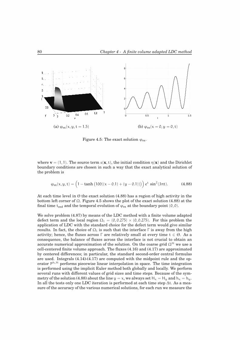
80 Chapter 4 - A finite volume adapted LDC method
0 0.5 1 1.5
0
2
4
6
8
t
(a) ϕex(x, y, t = 1.5) (b) ϕex(x = 0, y = 0, t)
Figure 4.5: The exact solution ϕex.
where v = (1, 1). The source term s(x, t), the initial condition η(x) and the Dirichlet
boundary conditions are chosen in such a way that the exact analytical solution of
the problem is
ϕex(x, y, t) =(
1− tanh(
100((x − 0.1) + (y− 0.1)))
)
et sin2(3πt). (4.88)
At each time level in Θ the exact solution (4.88) has a region of high activity in the
bottom left corner of Ω. Figure 4.5 shows the plot of the exact solution (4.88) at the
final time tend and the temporal evolution of ϕex at the boundary point (0, 0).
We solve problem (4.87) by means of the LDC method with a finite volume adapted
defect term and the local region Ωl = (0, 0.275) × (0, 0.275). For this problem the
application of LDC with the standard choice for the defect term would give similar
results. In fact, the choice of Ωl is such that the interface Γ is away from the high
activity; hence, the fluxes across Γ are relatively small at every time t ∈ Θ. As a
consequence, the balance of fluxes across the interface is not crucial to obtain an
accurate numerical approximation of the solution. On the coarse grid ΩH we use a
cell-centered finite volume approach. The fluxes (4.16) and (4.17) are approximated
by centered differences; in particular, the standard second-order central formulas
are used. Integrals (4.14)-(4.17) are computed with the midpoint rule and the op-
erator Ph,H performs piecewise linear interpolation in space. The time integration
is performed using the implicit Euler method both globally and locally. We perform
several runs with different values of grid sizes and time steps. Because of the sym-
metry of the solution (4.88) about the line y = x, we always setHx = Hy and hx = hy.
In all the tests only one LDC iteration is performed at each time step ∆t. As a mea-
sure of the accuracy of the various numerical solutions, for each run we measure the
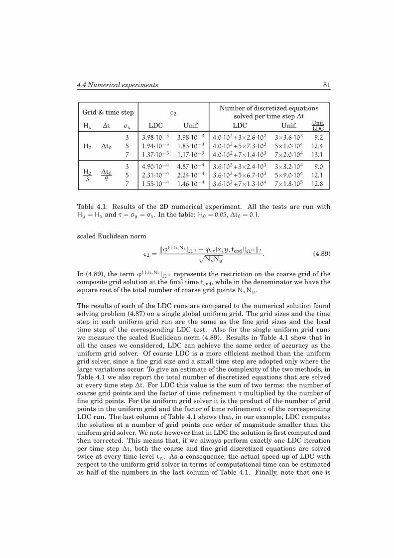
4.4 Numerical experiments 81
Grid & time step ǫ2Number of discretized equations
solved per time step ∆t
Hx ∆t σx LDC Unif. LDC Unif. Unif.LDC
3 3.98·10−3 3.98·10−3 4.0·102 +3×2.6·102 3×3.6·103 9.2
H0 ∆t0 5 1.94·10−3 1.83·10−3 4.0·102 +5×7.3·102 5×1.0·104 12.4
7 1.37·10−3 1.17·10−3 4.0·102 +7×1.4·103 7×2.0·104 13.1
H0
3∆t09
3 4.90·10−4 4.87·10−4 3.6·103 +3×2.4·103 3×3.2·104 9.0
5 2.31·10−4 2.24·10−4 3.6·103 +5×6.7·103 5×9.0·104 12.1
7 1.55·10−4 1.46·10−4 3.6·103 +7×1.3·104 7×1.8·105 12.8
Table 4.1: Results of the 2D numerical experiment. All the tests are run with
Hy = Hx and τ = σy = σx. In the table: H0 = 0.05, ∆t0 = 0.1.
scaled Euclidean norm
ǫ2 =‖ϕH,h,Nt |ΩH −ϕex(x, y, tend)|ΩH‖2
√
NxNy
. (4.89)
In (4.89), the term ϕH,h,Nt |ΩH represents the restriction on the coarse grid of the
composite grid solution at the final time tend, while in the denominator we have the
square root of the total number of coarse grid points NxNy.
The results of each of the LDC runs are compared to the numerical solution found
solving problem (4.87) on a single global uniform grid. The grid sizes and the time
step in each uniform grid run are the same as the fine grid sizes and the local
time step of the corresponding LDC test. Also for the single uniform grid runs
we measure the scaled Euclidean norm (4.89). Results in Table 4.1 show that in
all the cases we considered, LDC can achieve the same order of accuracy as the
uniform grid solver. Of course LDC is a more efficient method than the uniform
grid solver, since a fine grid size and a small time step are adopted only where the
large variations occur. To give an estimate of the complexity of the two methods, in
Table 4.1 we also report the total number of discretized equations that are solved
at every time step ∆t. For LDC this value is the sum of two terms: the number of
coarse grid points and the factor of time refinement τ multiplied by the number of
fine grid points. For the uniform grid solver it is the product of the number of grid
points in the uniform grid and the factor of time refinement τ of the corresponding
LDC run. The last column of Table 4.1 shows that, in our example, LDC computes
the solution at a number of grid points one order of magnitude smaller than the
uniform grid solver. We note however that in LDC the solution is first computed and
then corrected. This means that, if we always perform exactly one LDC iteration
per time step ∆t, both the coarse and fine grid discretized equations are solved
twice at every time level tn. As a consequence, the actual speed-up of LDC with
respect to the uniform grid solver in terms of computational time can be estimated
as half of the numbers in the last column of Table 4.1. Finally, note that one is
82 Chapter 4 - A finite volume adapted LDC method
not necessarily forced to set the factor of time refinement τ equal to the factors of
grid refinement σx and σy. For real applications one would rather first choose the
grid sizes and the time steps on the two grids so that both the global and the local
scales are properly resolved, and then set the factors of refinement consequently. In
general we expect τ to be neither too big nor too small with respect to the factors of
grid refinement. In the first case the spatial components of error might be dominant
in the local problem, while in the second case the local time scales might not be
properly resolved.
4.4.2 Example 2: comparison with the standard LDC method
In this section we present a two-dimensional problem for which conservation of
fluxes across the interface between coarse and fine grid plays a crucial rule. For
such a problem, we expect the finite volume adapted LDC algorithm to be more ac-
curate than the LDC method presented in [44], where no special precautions are
taken in order to guarantee conservation on the composite grid.
We choose Ω = (0, 2) × (0, 1) and Θ = (0, tend], with tend = 20, and we solve
∂ϕ
∂t+ ∇ ·
(
vϕ− ∇ϕ)
= 0, in Ω×Θ,
(
vϕ− ∇ϕ)
· n = 0, on ∂Ω×Θ,
ϕ = 1, in Ω, t = 0.
(4.90)
The velocity field is v = (vx, vy) = (1 + 5 sin(πt/2), 0.5 + 5 sin(πt/2)). The choice of
the boundary conditions is such that integration of the partial differential equation
over Ω yields the following global conservation law
d
dtM(t) = 0, (4.91)
where M(t) is defined by
M(t) :=
∫ ∫
Ω
ϕ(x, y, t) dx dy. (4.92)
The solution ϕ is periodic in time with period T = 4 and varies most in the regions
ofΩ next to the corners P0 = (0, 0) and P1 = (2, 1). The velocity field is such that the
amplitude of the oscillations in P1 is larger than in P0. Moreover the velocity field is
such that, unlike the example in Section 4.4.1, the solution is not symmetric about
the line y = x. Figure 4.6 shows the solution ϕ at two different time levels.
Because of the two local regions of high activity, problem (4.90) is solved by means
of LDC. On the global coarse grid we apply the finite volume method with a cell-
centered approach. As in the previous example, we approximate integrals by the
midpoint rule, and fluxes by second-order centered differences. Two local fine grids
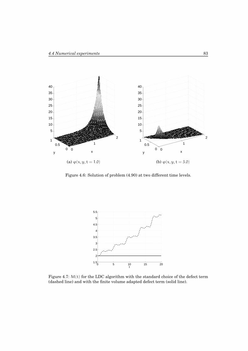
4.4 Numerical experiments 83
0
1
2
00.5
1
5
10
15
20
25
30
35
40
xy0
1
2
00.5
1
5
10
15
20
25
30
35
40
xy
(a) ϕ(x, y, t = 1.0) (b) ϕ(x, y, t = 3.0)
Figure 4.6: Solution of problem (4.90) at two different time levels.
0 5 10 15 201.5
2
2.5
3
3.5
4
4.5
5
5.5
t
Figure 4.7: M(t) for the LDC algorithm with the standard choice of the defect term
(dashed line) and with the finite volume adapted defect term (solid line).
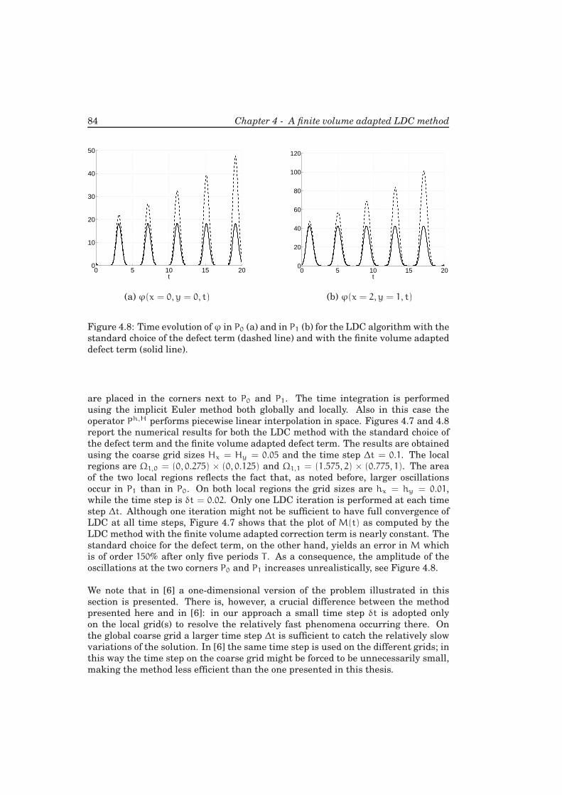
84 Chapter 4 - A finite volume adapted LDC method
0 5 10 15 200
10
20
30
40
50
t0 5 10 15 20
0
20
40
60
80
100
120
t
(a) ϕ(x = 0, y = 0, t) (b) ϕ(x = 2, y = 1, t)
Figure 4.8: Time evolution ofϕ in P0 (a) and in P1 (b) for the LDC algorithm with the
standard choice of the defect term (dashed line) and with the finite volume adapted
defect term (solid line).
are placed in the corners next to P0 and P1. The time integration is performed
using the implicit Euler method both globally and locally. Also in this case the
operator Ph,H performs piecewise linear interpolation in space. Figures 4.7 and 4.8
report the numerical results for both the LDC method with the standard choice of
the defect term and the finite volume adapted defect term. The results are obtained
using the coarse grid sizes Hx = Hy = 0.05 and the time step ∆t = 0.1. The local
regions are Ωl,0 = (0, 0.275) × (0, 0.125) and Ωl,1 = (1.575, 2) × (0.775, 1). The area
of the two local regions reflects the fact that, as noted before, larger oscillations
occur in P1 than in P0. On both local regions the grid sizes are hx = hy = 0.01,
while the time step is δt = 0.02. Only one LDC iteration is performed at each time
step ∆t. Although one iteration might not be sufficient to have full convergence of
LDC at all time steps, Figure 4.7 shows that the plot of M(t) as computed by the
LDC method with the finite volume adapted correction term is nearly constant. The
standard choice for the defect term, on the other hand, yields an error in M which
is of order 150% after only five periods T . As a consequence, the amplitude of the
oscillations at the two corners P0 and P1 increases unrealistically, see Figure 4.8.
We note that in [6] a one-dimensional version of the problem illustrated in this
section is presented. There is, however, a crucial difference between the method
presented here and in [6]: in our approach a small time step δt is adopted only
on the local grid(s) to resolve the relatively fast phenomena occurring there. On
the global coarse grid a larger time step ∆t is sufficient to catch the relatively slow
variations of the solution. In [6] the same time step is used on the different grids; in
this way the time step on the coarse grid might be forced to be unnecessarily small,
making the method less efficient than the one presented in this thesis.
Chapter 5
Generalizations of the LDCmethod
In Chapter 4 we introduced a finite volume adapted LDC algorithm such that the
computed composite grid solution satisfies a system of discrete conservation laws,
see Theorem 4.5. However, we restricted ourselves to cases where the high activity
of the solution is always located in the same limited part of the global domainΩ and
we did not include a regridding strategy in Algorithm 4.1. In this chapter we want
to overcome this limitation and we introduce a conservative regridding procedure to
be incorporated in the finite volume adapted LDC algorithm. The algorithm is then
extended to include multiple levels of refinement.
5.1 A conservative regridding strategy
In LDC, a regridding strategy is needed when the high activity of the solution is
located in different regions of the global domain at different time levels. In order to
properly resolve the local small scales of the solution and to avoid unnecessary re-
finement, the local fine grid has to be adapted to the solution’s behavior at each time
step. In Chapter 2 we explained that this can be done measuring certain features of
the first global approximation computed at the new time level. Once the new local
region has been chosen, initial values ϕH,h,n∗
are to be provided in all the points of
the new composite grid (see Algorithm 2.4) in order to perform the next LDC time
step.
Consider now the finite volume adapted LDC algorithm and assume that the solu-
tion’s high activity is located in different regions of the global domain Ω at differ-
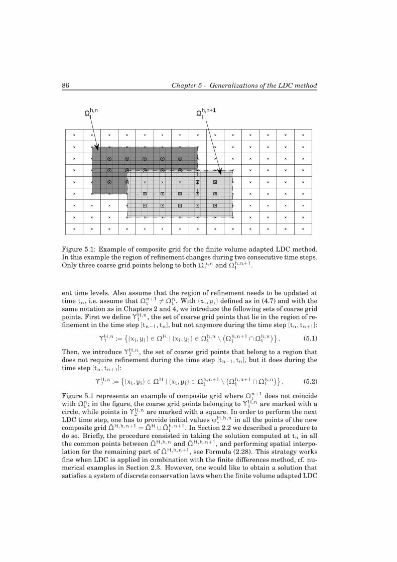
86 Chapter 5 - Generalizations of the LDC method
Ωh,nl
Ωh,n+1l
Figure 5.1: Example of composite grid for the finite volume adapted LDC method.
In this example the region of refinement changes during two consecutive time steps.
Only three coarse grid points belong to both Ωh,nl and Ωh,n+1
l .
ent time levels. Also assume that the region of refinement needs to be updated at
time tn, i.e. assume that Ωn+1l 6= Ωn
l . With (xi, yj) defined as in (4.7) and with the
same notation as in Chapters 2 and 4, we introduce the following sets of coarse grid
points. First we define ΥH,n1 , the set of coarse grid points that lie in the region of re-
finement in the time step [tn−1, tn], but not anymore during the time step [tn, tn+1]:
ΥH,n1 :=
(xi, yj) ∈ ΩH | (xi, yj) ∈ Ωh,n
l \(
Ωh,n+1l ∩Ωh,n
l
). (5.1)
Then, we introduce ΥH,n2 , the set of coarse grid points that belong to a region that
does not require refinement during the time step [tn−1, tn], but it does during the
time step [tn, tn+1]:
ΥH,n2 :=
(xi, yj) ∈ ΩH | (xi, yj) ∈ Ωh,n+1
l \(
Ωh,n+1l ∩Ωh,n
l
). (5.2)
Figure 5.1 represents an example of composite grid where Ωn+1l does not coincide
with Ωnl ; in the figure, the coarse grid points belonging to ΥH,n
1 are marked with a
circle, while points in ΥH,n2 are marked with a square. In order to perform the next
LDC time step, one has to provide initial values ϕH,h,n∗
in all the points of the new
composite grid ΩH,h,n+1 = ΩH ∪ Ωh,n+1l . In Section 2.2 we described a procedure to
do so. Briefly, the procedure consisted in taking the solution computed at tn in all
the common points between ΩH,h,n and ΩH,h,n+1, and performing spatial interpo-
lation for the remaining part of ΩH,h,n+1, see Formula (2.28). This strategy works
fine when LDC is applied in combination with the finite differences method, cf. nu-
merical examples in Section 2.3. However, one would like to obtain a solution that
satisfies a system of discrete conservation laws when the finite volume adapted LDC
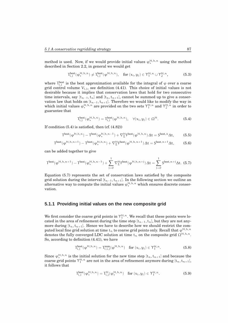
5.1 A conservative regridding strategy 87
method is used. Now, if we would provide initial values ϕH,h,n∗
using the method
described in Section 2.2, in general we would get
Tbesti,j (ϕH,h,n
∗) 6= Tbest
i,j (ϕH,h,n), for (xi, yj) ∈ ΥH,n1 ∪ ΥH,n
2 , (5.3)
where Tbesti,j is the best approximation available for the integral of ϕ over a coarse
grid control volume Vi,j, see definition (4.41). This choice of initial values is not
desirable because it implies that conservation laws that hold for two consecutive
time intervals, say [tn−1, tn] and [tn, tn+1], cannot be summed up to give a conser-
vation law that holds on [tn−1, tn+1]. Therefore we would like to modify the way in
which initial values ϕH,h,n∗
are provided on the two sets ΥH,n1 and ΥH,n
2 in order to
guarantee that
Tbesti,j (ϕH,h,n
∗) = Tbest
i,j (ϕH,h,n), ∀(xi, yj) ∈ ΩH. (5.4)
If condition (5.4) is satisfied, then (cf. (4.82))
Tbest(ϕH,h,n) − Tbest(ϕH,h,n−1∗
) + ∇HΣ F
best(ϕH,h,n)∆t = Sbest,n∆t, (5.5)
Tbest(ϕH,h,n+1) − Tbest(ϕH,h,n∗
) + ∇HΣ F
best(ϕH,h,n+1)∆t = Sbest,n+1∆t, (5.6)
can be added together to give
Tbest(ϕH,h,n+1) − Tbest(ϕH,h,n−1∗
) +
1∑
j=0
∇HΣ F
best(ϕH,h,n+j)∆t =
1∑
j=0
Sbest,n+j∆t. (5.7)
Equation (5.7) represents the set of conservation laws satisfied by the composite
grid solution during the interval [tn−1, tn+1]. In the following section we outline an
alternative way to compute the initial values ϕH,h,n∗
which ensures discrete conser-
vation.
5.1.1 Providing initial values on the new composite grid
We first consider the coarse grid points in ΥH,n1 . We recall that these points were lo-
cated in the area of refinement during the time step [tn−1, tn], but they are not any-
more during [tn, tn+1]. Hence we have to describe how we should restrict the com-
puted local fine grid solution at time tn to coarse grid points only. Recall that ϕH,h,n
denotes the fully converged LDC solution at time tn on the composite grid ΩH,h,n.
So, according to definition (4.41), we have
Tbesti,j (ϕH,h,n) = T sum
l,i,j(ϕH,h,n) for (xi, yj) ∈ ΥH,n
1 . (5.8)
Since ϕH,h,n∗
is the initial solution for the new time step [tn, tn+1] and because the
coarse grid points ΥH,n1 are not in the area of refinement anymore during [tn, tn+1],
it follows that
Tbesti,j (ϕH,h,n
∗) = TH
i,j(ϕH,h,n∗
) for (xi, yj) ∈ ΥH,n1 . (5.9)
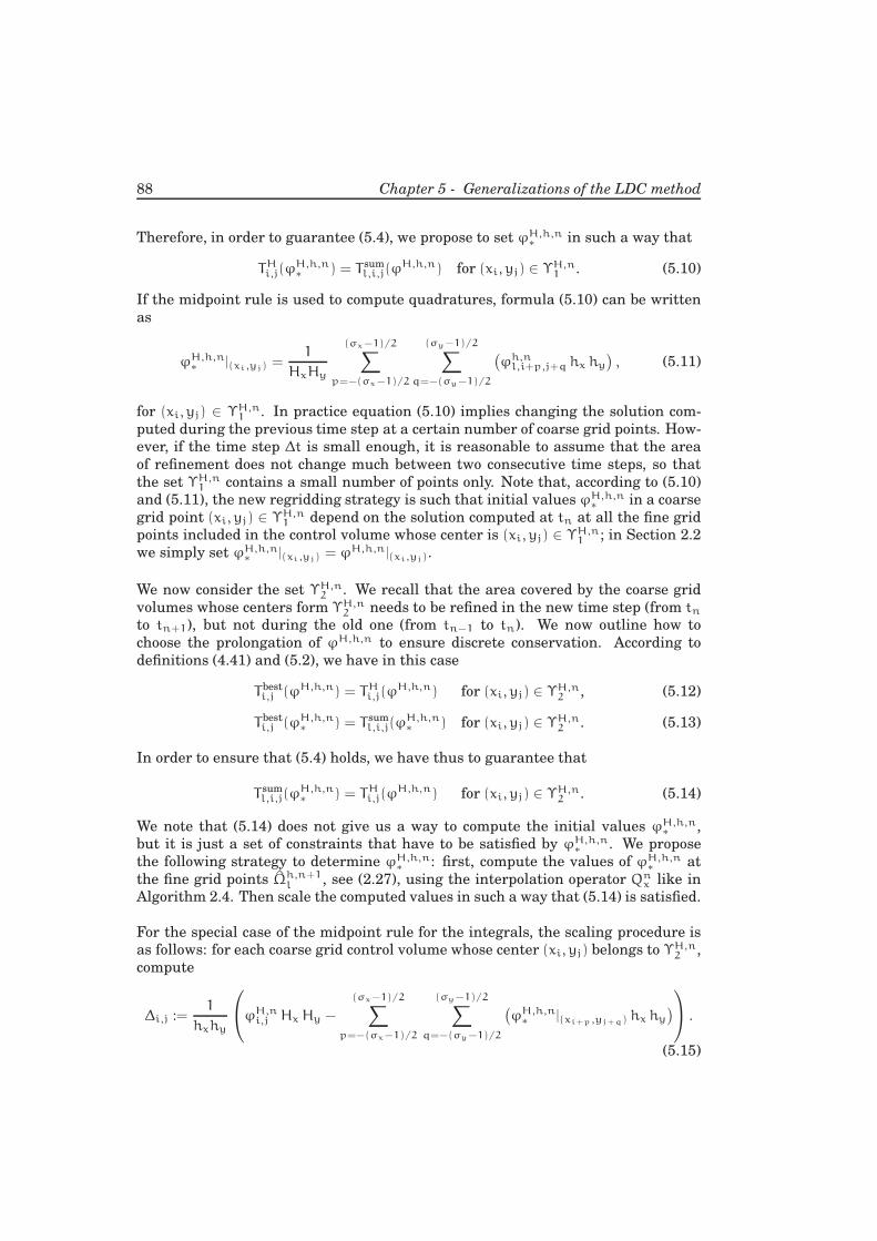
88 Chapter 5 - Generalizations of the LDC method
Therefore, in order to guarantee (5.4), we propose to set ϕH,h,n∗
in such a way that
THi,j(ϕ
H,h,n∗
) = T suml,i,j(ϕ
H,h,n) for (xi, yj) ∈ ΥH,n1 . (5.10)
If the midpoint rule is used to compute quadratures, formula (5.10) can be written
as
ϕH,h,n∗
|(xi,yj) =1
HxHy
(σx−1)/2∑
p=−(σx−1)/2
(σy−1)/2∑
q=−(σy−1)/2
(
ϕh,nl,i+p,j+q hx hy
)
, (5.11)
for (xi, yj) ∈ ΥH,n1 . In practice equation (5.10) implies changing the solution com-
puted during the previous time step at a certain number of coarse grid points. How-
ever, if the time step ∆t is small enough, it is reasonable to assume that the area
of refinement does not change much between two consecutive time steps, so that
the set ΥH,n1 contains a small number of points only. Note that, according to (5.10)
and (5.11), the new regridding strategy is such that initial values ϕH,h,n∗
in a coarse
grid point (xi, yj) ∈ ΥH,n1 depend on the solution computed at tn at all the fine grid
points included in the control volume whose center is (xi, yj) ∈ ΥH,n1 ; in Section 2.2
we simply set ϕH,h,n∗
|(xi,yj) = ϕH,h,n|(xi,yj).
We now consider the set ΥH,n2 . We recall that the area covered by the coarse grid
volumes whose centers form ΥH,n2 needs to be refined in the new time step (from tn
to tn+1), but not during the old one (from tn−1 to tn). We now outline how to
choose the prolongation of ϕH,h,n to ensure discrete conservation. According to
definitions (4.41) and (5.2), we have in this case
Tbesti,j (ϕH,h,n) = TH
i,j(ϕH,h,n) for (xi, yj) ∈ ΥH,n
2 , (5.12)
Tbesti,j (ϕH,h,n
∗) = T sum
l,i,j(ϕH,h,n∗
) for (xi, yj) ∈ ΥH,n2 . (5.13)
In order to ensure that (5.4) holds, we have thus to guarantee that
T suml,i,j(ϕ
H,h,n∗
) = THi,j(ϕ
H,h,n) for (xi, yj) ∈ ΥH,n2 . (5.14)
We note that (5.14) does not give us a way to compute the initial values ϕH,h,n∗
,
but it is just a set of constraints that have to be satisfied by ϕH,h,n∗
. We propose
the following strategy to determine ϕH,h,n∗
: first, compute the values of ϕH,h,n∗
at
the fine grid points Ωh,n+1l , see (2.27), using the interpolation operator Qn
x like in
Algorithm 2.4. Then scale the computed values in such a way that (5.14) is satisfied.
For the special case of the midpoint rule for the integrals, the scaling procedure is
as follows: for each coarse grid control volume whose center (xi, yj) belongs to ΥH,n2 ,
compute
∆i,j :=1
hxhy
ϕH,ni,j HxHy −
(σx−1)/2∑
p=−(σx−1)/2
(σy−1)/2∑
q=−(σy−1)/2
(
ϕH,h,n∗
|(xi+p,yj+q) hx hy
)
.
(5.15)
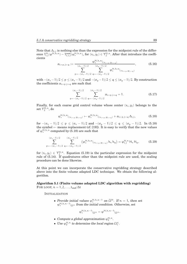
5.1 A conservative regridding strategy 89
Note that ∆i,j is nothing else than the expression for the midpoint rule of the differ-
ence THi,j(ϕ
H,h,n) − T suml,i,j(ϕ
H,h,n∗
), for (xi, yj) ∈ ΥH,n2 . After that introduce the coeffi-
cients
αi+p,j+q :=ϕH,h,n
∗|(xi+p,yj+q)
(σx−1)/2∑
p=−(σx−1)/2
(σy−1)/2∑
q=−(σy−1)/2
ϕH,h,n∗
|(xi+p,yj+q)
, (5.16)
with −(σx − 1)/2 ≤ p ≤ (σx − 1)/2 and −(σy − 1)/2 ≤ q ≤ (σy − 1)/2. By construction
the coefficients αi+p,j+q are such that
(σx−1)/2∑
p=−(σx−1)/2
(σy−1)/2∑
q=−(σy−1)/2
αi+p,j+q = 1. (5.17)
Finally, for each coarse grid control volume whose center (xi, yj) belongs to the
set ΥH,n2 , do
ϕH,h,n∗
|(xi+p,yj+q) ← ϕH,h,n∗
|(xi+p,yj+q) + αi+p,j+q∆i,j, (5.18)
for −(σx − 1)/2 ≤ p ≤ (σx − 1)/2 and −(σy − 1)/2 ≤ q ≤ (σy − 1)/2. In (5.18)
the symbol← means replacement (cf. [19]). It is easy to verify that the new values
of ϕH,h,n∗
computed by (5.18) are such that
(σx−1)/2∑
p=−(σx−1)/2
(σy−1)/2∑
q=−(σy−1)/2
(
ϕH,h,n∗
|(xi+p,yj+q) hx hy
)
= ϕH,ni,j HxHy, (5.19)
for (xi, yj) ∈ ΥH,n2 . Equation (5.19) is the particular expression for the midpoint
rule of (5.14). If quadratures other than the midpoint rule are used, the scaling
procedure can be done likewise.
At this point we can incorporate the conservative regridding strategy described
above into the finite volume adapted LDC technique. We obtain the following al-
gorithm.
Algorithm 5.1 (Finite volume adapted LDC algorithm with regridding)
FOR LOOP, n = 1, 2, . . . , tend/∆t
INITIALIZATION
• Provide initial values ϕH,h,n−1∗
on ΩH. If n = 1, then set
ϕH,h,n−1∗
|ΩH from the initial condition. Otherwise, set
ϕH,h,n−1∗
|ΩH = ϕH,h,n−1|ΩH .
• Compute a global approximation ϕH,n0 .
• Use ϕH,n0 to determine the local regionΩn
l .
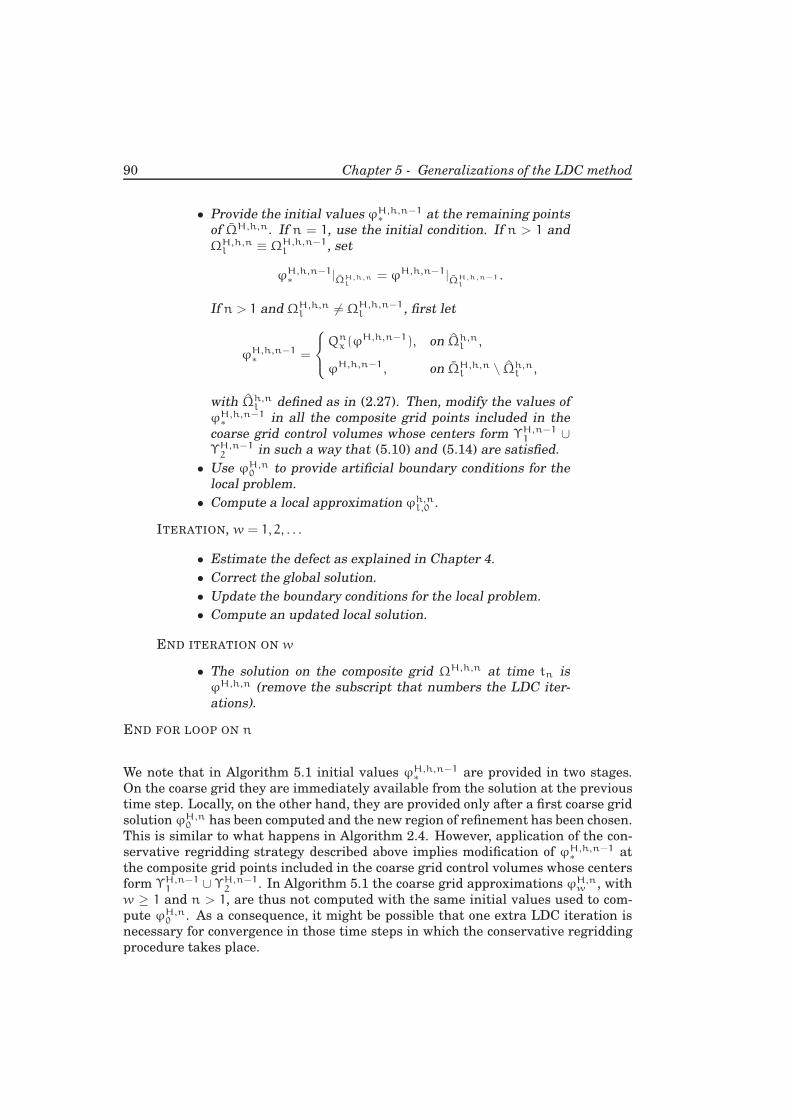
90 Chapter 5 - Generalizations of the LDC method
• Provide the initial values ϕH,h,n−1∗
at the remaining pointsof ΩH,h,n. If n = 1, use the initial condition. If n > 1 and
ΩH,h,nl ≡ ΩH,h,n−1
l , set
ϕH,h,n−1∗
|ΩH,h,nl
= ϕH,h,n−1|ΩH,h,n−1l
.
If n > 1 and ΩH,h,nl 6= ΩH,h,n−1
l , first let
ϕH,h,n−1∗
=
Qn
x (ϕH,h,n−1), on Ωh,nl ,
ϕH,h,n−1, on ΩH,h,nl \ Ωh,n
l ,
with Ωh,nl defined as in (2.27). Then, modify the values of
ϕH,h,n−1∗
in all the composite grid points included in the
coarse grid control volumes whose centers form ΥH,n−11 ∪
ΥH,n−12 in such a way that (5.10) and (5.14) are satisfied.
• Use ϕH,n0 to provide artificial boundary conditions for the
local problem.
• Compute a local approximation ϕh,nl,0 .
ITERATION, w = 1, 2, . . .
• Estimate the defect as explained in Chapter 4.
• Correct the global solution.
• Update the boundary conditions for the local problem.
• Compute an updated local solution.
END ITERATION ON w
• The solution on the composite grid ΩH,h,n at time tn isϕH,h,n (remove the subscript that numbers the LDC iter-
ations).
END FOR LOOP ON n
We note that in Algorithm 5.1 initial values ϕH,h,n−1∗
are provided in two stages.
On the coarse grid they are immediately available from the solution at the previous
time step. Locally, on the other hand, they are provided only after a first coarse grid
solution ϕH,n0 has been computed and the new region of refinement has been chosen.
This is similar to what happens in Algorithm 2.4. However, application of the con-
servative regridding strategy described above implies modification of ϕH,h,n−1∗
at
the composite grid points included in the coarse grid control volumes whose centers
form ΥH,n−11 ∪ ΥH,n−1
2 . In Algorithm 5.1 the coarse grid approximations ϕH,nw , with
w ≥ 1 and n > 1, are thus not computed with the same initial values used to com-
pute ϕH,n0 . As a consequence, it might be possible that one extra LDC iteration is
necessary for convergence in those time steps in which the conservative regridding
procedure takes place.
5.1 A conservative regridding strategy 91
5.1.2 A numerical example
In this section we test the conservative regridding strategy introduced above in a
concrete example and we compare it to the procedure described in Section 2.2. We
choose Ω = (0, 1)2 and Θ = (0, tend], with tend = 3, and we consider the following
two-dimensional convection-diffusion problem
∂u
∂t+ v · ∇u = λ∇2u, in Ω×Θ,
∇u · n = 0, on ∂Ω×Θ,
u = 100 exp(
−50(
(x − 0.3)2
+ (y− 0.8)2))
, in Ω, t = 0.
(5.20)
In (5.20), by n we denoted the outward unit vector perpendicular to ∂Ω. The diffu-
sion coefficient and the velocity field are chosen as λ = 10−3 and
v =(
− 2x (x− 1) (y− 0.5) , 2y (y− 1 )( x − 0.5))
, (5.21)
respectively. It is easy to verify the ∇ · v = 0. In this way problem (5.20) can be
written in integral formulation and solved using the finite volume adapted LDC
method. On the global grid we use a cell-centered approach. Both globally and
locally we approximate integrals by the midpoint rule, and fluxes by second-order
central formulas. Time discretization is performed by the backward Euler scheme
on both grids. In this example we let the operator Ph,H perform piecewise quadratic
interpolation.
The high activity of u is not confined to the same limited part ofΩ for all times t ∈ Θ.
Therefore we incorporate a regridding strategy in the finite volume adapted LDC
algorithm. At every time step, the local region Ωnl is determined using the method
described in [10, 11, 65]. For that we use a threshold value ǫ = 3, see Section 2.2.
We run two kinds of experiments: in the first one initial values ϕH,h,n∗
on ΩH,h,n+1
are prescribed using the regridding strategy discussed in Section 2.2; in the second
one we apply the conservative regridding method described in this chapter. In both
cases we let the operator Qnx perform piecewise quadratic interpolation from the
coarse grid solution.
We note that v · n = 0 on ∂Ω, and that homogeneous Neumann boundary conditions
are prescribed on the whole boundary. This yields to the fact that the following
identity holdsd
dtM(t) = 0, (5.22)
with
M(t) :=
∫ ∫
Ω
udx dy. (5.23)
In our experiments we want to test how well the two regridding strategies can re-
produce the conservation law (5.22). The results are plotted in Figure 5.2. They are
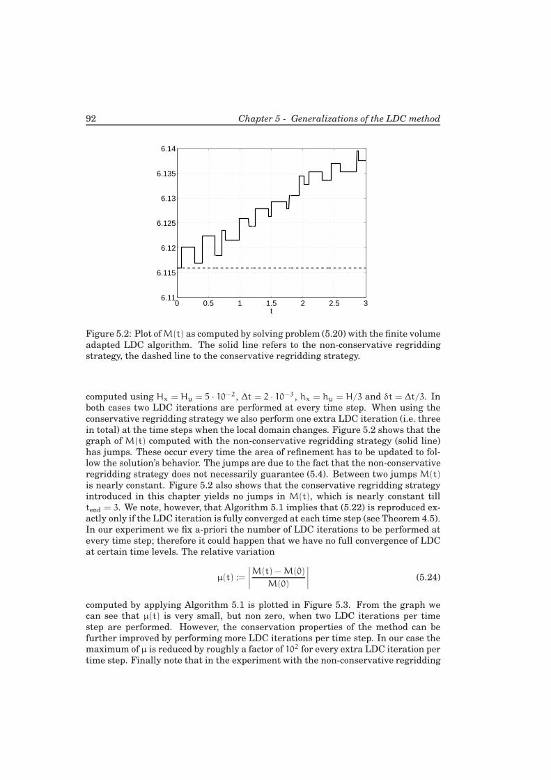
92 Chapter 5 - Generalizations of the LDC method
0 0.5 1 1.5 2 2.5 36.11
6.115
6.12
6.125
6.13
6.135
6.14
t
Figure 5.2: Plot ofM(t) as computed by solving problem (5.20) with the finite volume
adapted LDC algorithm. The solid line refers to the non-conservative regridding
strategy, the dashed line to the conservative regridding strategy.
computed using Hx = Hy = 5 · 10−2, ∆t = 2 · 10−3, hx = hy = H/3 and δt = ∆t/3. In
both cases two LDC iterations are performed at every time step. When using the
conservative regridding strategy we also perform one extra LDC iteration (i.e. three
in total) at the time steps when the local domain changes. Figure 5.2 shows that the
graph of M(t) computed with the non-conservative regridding strategy (solid line)
has jumps. These occur every time the area of refinement has to be updated to fol-
low the solution’s behavior. The jumps are due to the fact that the non-conservative
regridding strategy does not necessarily guarantee (5.4). Between two jumps M(t)
is nearly constant. Figure 5.2 also shows that the conservative regridding strategy
introduced in this chapter yields no jumps in M(t), which is nearly constant till
tend = 3. We note, however, that Algorithm 5.1 implies that (5.22) is reproduced ex-
actly only if the LDC iteration is fully converged at each time step (see Theorem 4.5).
In our experiment we fix a-priori the number of LDC iterations to be performed at
every time step; therefore it could happen that we have no full convergence of LDC
at certain time levels. The relative variation
µ(t) :=
∣
∣
∣
∣
M(t) −M(0)
M(0)
∣
∣
∣
∣
(5.24)
computed by applying Algorithm 5.1 is plotted in Figure 5.3. From the graph we
can see that µ(t) is very small, but non zero, when two LDC iterations per time
step are performed. However, the conservation properties of the method can be
further improved by performing more LDC iterations per time step. In our case the
maximum of µ is reduced by roughly a factor of 102 for every extra LDC iteration per
time step. Finally note that in the experiment with the non-conservative regridding
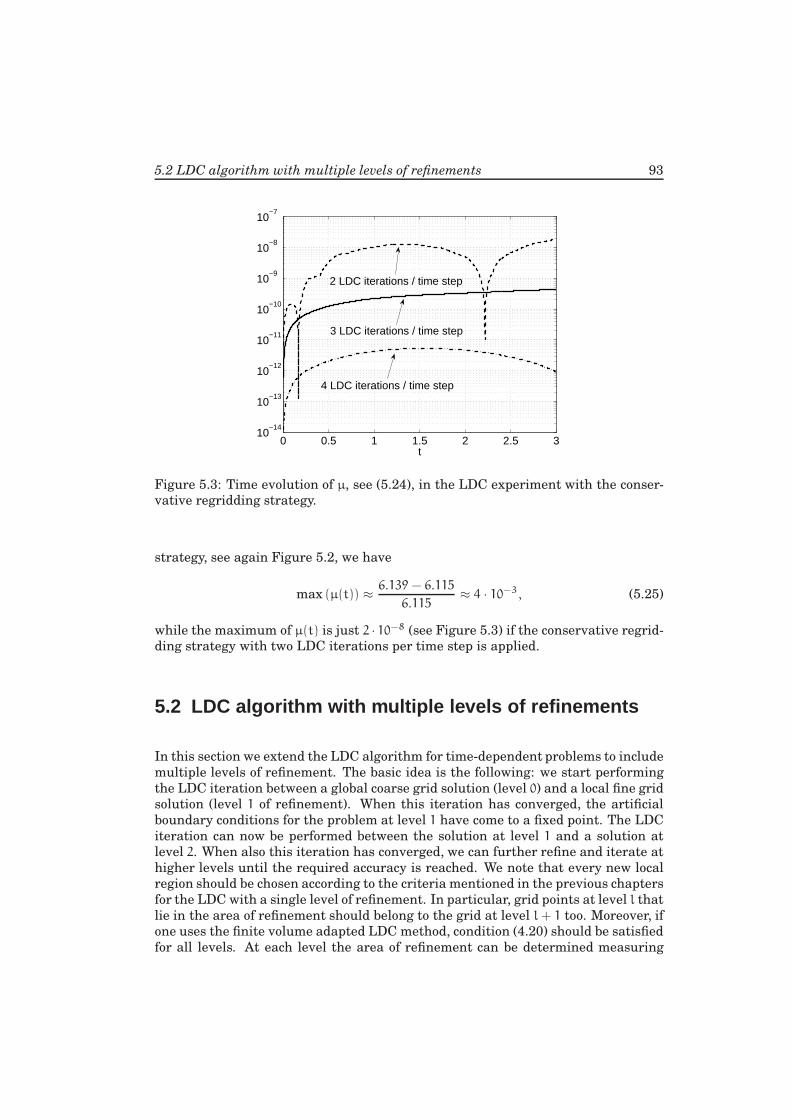
5.2 LDC algorithm with multiple levels of refinements 93
0 0.5 1 1.5 2 2.5 310
−14
10−13
10−12
10−11
10−10
10−9
10−8
10−7
t
2 LDC iterations / time step
3 LDC iterations / time step
4 LDC iterations / time step
Figure 5.3: Time evolution of µ, see (5.24), in the LDC experiment with the conser-
vative regridding strategy.
strategy, see again Figure 5.2, we have
max (µ(t)) ≈ 6.139 − 6.115
6.115≈ 4 · 10−3, (5.25)
while the maximum of µ(t) is just 2 · 10−8 (see Figure 5.3) if the conservative regrid-
ding strategy with two LDC iterations per time step is applied.
5.2 LDC algorithm with multiple levels of refinements
In this section we extend the LDC algorithm for time-dependent problems to include
multiple levels of refinement. The basic idea is the following: we start performing
the LDC iteration between a global coarse grid solution (level 0) and a local fine grid
solution (level 1 of refinement). When this iteration has converged, the artificial
boundary conditions for the problem at level 1 have come to a fixed point. The LDC
iteration can now be performed between the solution at level 1 and a solution at
level 2. When also this iteration has converged, we can further refine and iterate at
higher levels until the required accuracy is reached. We note that every new local
region should be chosen according to the criteria mentioned in the previous chapters
for the LDC with a single level of refinement. In particular, grid points at level l that
lie in the area of refinement should belong to the grid at level l+ 1 too. Moreover, if
one uses the finite volume adapted LDC method, condition (4.20) should be satisfied
for all levels. At each level the area of refinement can be determined measuring
94 Chapter 5 - Generalizations of the LDC method
certain features of the solution at that level; for instance, the method described
in [10, 11, 65] can be employed.
We observe that at each sublevel not only a finer grid spacing, but also a smaller
time step is adopted. The LDC time marching has to take this into account. In Fig-
ure 5.4 the procedure to perform one LDC time step with two levels of refinement is
illustrated. The figure refers to a case in which one and only one LDC iteration is
performed at each level, and the factor of time refinement is always τ = 2. Like in
the LDC method with a single level of refinement, the first step of the algorithm is
the computation of a first global solution (level 0) at tn (a). This provides artificial
boundary conditions to a local problem at level 1, which is then integrated from tn−1
till tn (b). The solution at level 0 is now improved by a defect correction (c). By as-
sumption the boundary conditions for the problem at level 1 have already reached a
fixed point. If this should not be the case, we could perform more iterations between
level 0 and level 1. The next step is anyhow applying the LDC method between
level 1 and level 2. For that we integrate the level 1 problem from tn−1 till tn−1/2 (d)
and we provide artificial boundary conditions for a problem at level 2. This is then
solved (e) and, after that, the level 1 solution at tn−1/2 is improved by a defect
correction (f). We move on by solving the level 2 problem with updated boundary
conditions and performing the second half time step at level 1 (e). The LDC itera-
tion is now performed between tn−1/2 and tn. A level 2 problem is solved (h), the
solution at level 1 is corrected (i) and finally the solution at the finest level is re-
computed with updated boundary conditions (j). This procedure defines a composite
grid solution at time tn.
We would like to remind here that one is not forced to use the same numerical
schemes at each level. Also the factors of grid and time refinement can be different
at different levels. The only requirement is that no explicit schemes are used at all
levels except at the finest. As noted before (Section 2.2), this is for the effectiveness
of the defect correction. We also want to highlight the following: if the finite volume
adapted LDC method is applied at each level in combination with the conservative
regridding strategy described in Section 5.1, the resulting solution turns out to be
conservative in a discrete sense on the multilevel composite grid, union of the global
and all the locally nested grids. This is not verified in a practical example here, but
it will become clear from the numerical experiments discussed in the next chapter.
Finally, note that in [1, 3] LDC is applied to solve a stationary combustion problem
and multiple levels of refinement are adopted. The approach there consists in com-
puting first an approximation of the solution on all grids, from the coarsest to the
finest level. After that, the solution on the finer grids is used to update the solution
on the coarser grids through a defect correction; this is done in an opposite order, i.e.
from the finest till the coarsest level. The entire cycle is then repeated again until a
fixed point in the iteration is reached. This approach is efficient (see numerical re-
sults in [1, 3]) for stationary problems. However, it does not have a straightforward
generalization to time-dependent partial differential equations that are solved lo-
cally not only with a finer grid size, but also with a smaller time step. For this
reason we proposed an approach that consists in iterating till convergence at a cer-
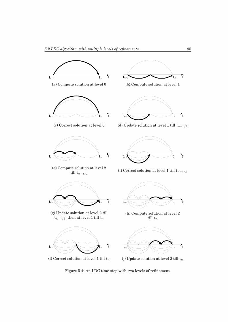
5.2 LDC algorithm with multiple levels of refinements 95
tntn−1 t tntn−1 t
(a) Compute solution at level 0 (b) Compute solution at level 1
tntn−1 t tntn−1 t
(c) Correct solution at level 0 (d) Update solution at level 1 till tn−1/2
tntn−1 t tntn−1 t
(e) Compute solution at level 2
till tn−1/2(f) Correct solution at level 1 till tn−1/2
tntn−1 t tntn−1 t
(g) Update solution at level 2 till
tn−1/2, then at level 1 till tn
(h) Compute solution at level 2
till tn
tntn−1 t tntn−1 t
(i) Correct solution at level 1 till tn (j) Update solution at level 2 till tn
Figure 5.4: An LDC time step with two levels of refinement.

96 Chapter 5 - Generalizations of the LDC method
tain level before moving on to a finer one.
With the new features introduced in this chapter, namely multiple levels of refine-
ment and a conservative regridding strategy, the LDC method is now complete and
can be used to solve realistic physical problems. The following chapter is concerned
with the solution of transport problems in transient flow fields by means of LDC.
Chapter 6
Solving transport problemsusing LDC
In this chapter, we will consider the transport of passive tracers in a given velocity
field. A passive tracer is a diffusive contaminant in a fluid flow that is present in
such low concentration that it does not influence the dynamics of the flow. Under-
standing the influence of the main flow on the tracer material is crucial in many
engineering applications, such as mixing in chemical reactors or transport of fly
ashes in burners. Knowledge of the passive tracer behavior is also of fundamen-
tal importance in enviromental sciences for studying dispersion of pollutants (e.g.
chemical species, radioactive components) in the atmosphere or in the oceans.
Transport of passive tracers is modeled by an advection-diffusion equation, and it
has been studied from a phenomenological and experimental point of view by many
authors, see review articles [26, 52, 67] and references therein. In turbulent flows,
one of the main difficulties of the problem from a computational point of view is the
scale separation between main flow eddies and transport processes: the latter occur
at a scale which can be a few times smaller than the smallest length scales of the
turbulent flow [26]. Considering the fact that running Direct Numerical Simula-
tions (DNS) of the main flow is already challenging in simple geometries, but still
feasible using for example spectral methods, we see that it is much more difficult to
properly simulate the transport processes. In many practical applications, however,
the tracer material is mainly confined in a very limited part of the computational
domain. The LDC method for time-dependent PDEs we developed in the previous
chapters seems thus to be an appealing technique for solving the transport problem.
Using LDC, in fact, a fine grid spacing and a small time step can be adopted only
where the highest concentration of the tracer material occurs. Moreover, when the
LDC iteration is fully converged, the finite volume adapted LDC method in combina-
tion with a conservative regridding strategy guarantees conservation of the tracer
98 Chapter 6 - Solving transport problems using LDC
material. In this chapter we study a test problem in which the main flow equations
are still solved by spectral methods, while the solution of the transport problem is
computed on composite grids by means of LDC.
6.1 Mathematical model
We consider a dipole-wall collision problem in the two-dimensional spatial domain
Ω = (0, 2) × (−1, 1). In this test case a velocity dipole is initially located at the
center of the domain Ω and it starts travelling towards one of the walls. After a
certain time the dipole hits the wall and secondary vortices are formed. We place
some tracer material around the point where the dipole hits the wall, and we run
simulations to see how the tracer detaches from the wall and is transported by the
velocity field.
We indicate by ϕ(x, y, t) the continuous distribution of the passive tracer, and by
v(x, y, t) the given velocity field. The transport of the passive tracer is modeled by
the following dimensionless advection-diffusion equation
∂ϕ
∂t+ v · ∇ϕ =
1
Pe∇2ϕ, in Ω. (6.1)
In (6.1), the Peclet number is defined as Pe := V D/k, where V is a characteristic
velocity of the flow, D the half-width of the rectangular domain Ω (i.e. D = 1 in
our case) and k the tracer’s molecular diffusivity. Approach (6.1) is called Eulerian
in contrast with the Lagrangian approach, where trajectories of individual tracer
particles are computed, see [56]. Partial differential equation (6.1) is solved with
the no-flux boundary condition
∇ϕ · n = 0, on ∂Ω, (6.2)
where n is the outward unit vector perpendicular to the boundary. The initial con-
dition for ϕ is the Gaussian distribution
ϕ(x, y, t = 0) =1
2πσ20
exp
(
−(x− 1.0)
2+ (y+ 1.0)
2
2σ20
)
, (6.3)
with σ0 = 0.1/√2. The Gaussian distribution (6.3) is centered in the point (1.0,−1.0)
and about 95% of the tracer material is confined within a distance of 2σ0 ≈ 0.14 from
the center of the distribution.
For solving advection-diffusion equation (6.1), the velocity field v must be given. In
practice, v(x, y, t) is computed solving the two-dimensional Navier-Stokes equations
in the velocity-vorticity formulation. This system includes the following dimension-
less equation for the vorticity ω(x, y, t)
∂ω
∂t+ v · ∇ω =
1
Re∇2ω, in Ω. (6.4)
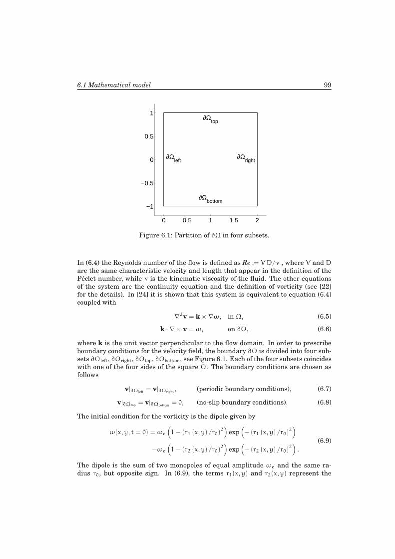
6.1 Mathematical model 99
0 0.5 1 1.5 2
−1
−0.5
0
0.5
1
∂Ωbottom
∂Ωtop
∂Ωleft
∂Ωright
Figure 6.1: Partition of ∂Ω in four subsets.
In (6.4) the Reynolds number of the flow is defined as Re := V D/ν , where V and D
are the same characteristic velocity and length that appear in the definition of the
Peclet number, while ν is the kinematic viscosity of the fluid. The other equations
of the system are the continuity equation and the definition of vorticity (see [22]
for the details). In [24] it is shown that this system is equivalent to equation (6.4)
coupled with
∇2v = k ×∇ω, in Ω, (6.5)
k · ∇ × v = ω, on ∂Ω, (6.6)
where k is the unit vector perpendicular to the flow domain. In order to prescribe
boundary conditions for the velocity field, the boundary ∂Ω is divided into four sub-
sets ∂Ωleft, ∂Ωright, ∂Ωtop, ∂Ωbottom, see Figure 6.1. Each of the four subsets coincides
with one of the four sides of the square Ω. The boundary conditions are chosen as
follows
v|∂Ωleft= v|∂Ωright
, (periodic boundary conditions), (6.7)
v|∂Ωtop= v|∂Ωbottom
= 0, (no-slip boundary conditions). (6.8)
The initial condition for the vorticity is the dipole given by
ω(x, y, t = 0) = ωe
(
1− (r1 (x, y) /r0)2)
exp(
− (r1 (x, y) /r0)2)
−ωe
(
1− (r2 (x, y) /r0)2)
exp(
− (r2 (x, y) /r0)2)
.
(6.9)
The dipole is the sum of two monopoles of equal amplitude ωe and the same ra-
dius r0, but opposite sign. In (6.9), the terms r1(x, y) and r2(x, y) represent the
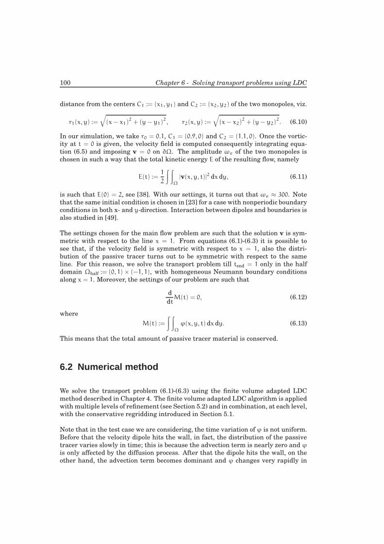
100 Chapter 6 - Solving transport problems using LDC
distance from the centers C1 := (x1, y1) and C2 := (x2, y2) of the two monopoles, viz.
r1(x, y) :=
√
(x− x1)2
+ (y− y1)2, r2(x, y) :=
√
(x− x2)2
+ (y− y2)2. (6.10)
In our simulation, we take r0 = 0.1, C1 = (0.9, 0) and C2 = (1.1, 0). Once the vortic-
ity at t = 0 is given, the velocity field is computed consequently integrating equa-
tion (6.5) and imposing v = 0 on ∂Ω. The amplitude ωe of the two monopoles is
chosen in such a way that the total kinetic energy E of the resulting flow, namely
E(t) :=1
2
∫ ∫
Ω
|v(x, y, t)|2 dx dy, (6.11)
is such that E(0) = 2, see [38]. With our settings, it turns out that ωe ≈ 300. Note
that the same initial condition is chosen in [23] for a case with nonperiodic boundary
conditions in both x- and y-direction. Interaction between dipoles and boundaries is
also studied in [49].
The settings chosen for the main flow problem are such that the solution v is sym-
metric with respect to the line x = 1. From equations (6.1)-(6.3) it is possible to
see that, if the velocity field is symmetric with respect to x = 1, also the distri-
bution of the passive tracer turns out to be symmetric with respect to the same
line. For this reason, we solve the transport problem till tend = 1 only in the half
domain Ωhalf := (0, 1) × (−1, 1), with homogeneous Neumann boundary conditions
along x = 1. Moreover, the settings of our problem are such that
d
dtM(t) = 0, (6.12)
where
M(t) :=
∫ ∫
Ω
ϕ(x, y, t) dx dy. (6.13)
This means that the total amount of passive tracer material is conserved.
6.2 Numerical method
We solve the transport problem (6.1)-(6.3) using the finite volume adapted LDC
method described in Chapter 4. The finite volume adapted LDC algorithm is applied
with multiple levels of refinement (see Section 5.2) and in combination, at each level,
with the conservative regridding introduced in Section 5.1.
Note that in the test case we are considering, the time variation of ϕ is not uniform.
Before that the velocity dipole hits the wall, in fact, the distribution of the passive
tracer varies slowly in time; this is because the advection term is nearly zero and ϕ
is only affected by the diffusion process. After that the dipole hits the wall, on the
other hand, the advection term becomes dominant and ϕ changes very rapidly in
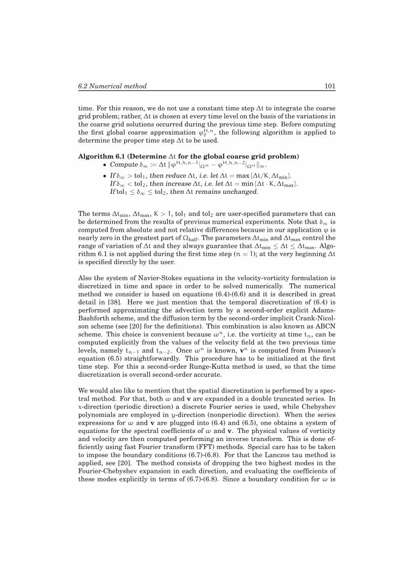
6.2 Numerical method 101
time. For this reason, we do not use a constant time step ∆t to integrate the coarse
grid problem; rather, ∆t is chosen at every time level on the basis of the variations in
the coarse grid solutions occurred during the previous time step. Before computing
the first global coarse approximation ϕH,n0 , the following algorithm is applied to
determine the proper time step ∆t to be used.
Algorithm 6.1 (Determine ∆t for the global coarse grid problem)
• Compute δ∞ := ∆t ‖ϕH,h,n−1|ΩH −ϕH,h,n−2|ΩH‖∞ .
• If δ∞ > tol1, then reduce ∆t, i.e. let ∆t = max ∆t/K,∆tmin.
If δ∞ < tol2, then increase ∆t, i.e. let ∆t = min ∆t · K,∆tmax.If tol1 ≤ δ∞ ≤ tol2, then ∆t remains unchanged.
The terms ∆tmin, ∆tmax, K > 1, tol1 and tol2 are user-specified parameters that can
be determined from the results of previous numerical experiments. Note that δ∞ is
computed from absolute and not relative differences because in our application ϕ is
nearly zero in the greatest part ofΩhalf. The parameters ∆tmin and ∆tmax control the
range of variation of ∆t and they always guarantee that ∆tmin ≤ ∆t ≤ ∆tmax. Algo-
rithm 6.1 is not applied during the first time step (n = 1); at the very beginning ∆t
is specified directly by the user.
Also the system of Navier-Stokes equations in the velocity-vorticity formulation is
discretized in time and space in order to be solved numerically. The numerical
method we consider is based on equations (6.4)-(6.6) and it is described in great
detail in [38]. Here we just mention that the temporal discretization of (6.4) is
performed approximating the advection term by a second-order explicit Adams-
Bashforth scheme, and the diffusion term by the second-order implicit Crank-Nicol-
son scheme (see [20] for the definitions). This combination is also known as ABCN
scheme. This choice is convenient because ωn, i.e. the vorticity at time tn, can be
computed explicitly from the values of the velocity field at the two previous time
levels, namely tn−1 and tn−2. Once ωn is known, vn is computed from Poisson’s
equation (6.5) straightforwardly. This procedure has to be initialized at the first
time step. For this a second-order Runge-Kutta method is used, so that the time
discretization is overall second-order accurate.
We would also like to mention that the spatial discretization is performed by a spec-
tral method. For that, both ω and v are expanded in a double truncated series. In
x-direction (periodic direction) a discrete Fourier series is used, while Chebyshev
polynomials are employed in y-direction (nonperiodic direction). When the series
expressions for ω and v are plugged into (6.4) and (6.5), one obtains a system of
equations for the spectral coefficients of ω and v. The physical values of vorticity
and velocity are then computed performing an inverse transform. This is done ef-
ficiently using fast Fourier transform (FFT) methods. Special care has to be taken
to impose the boundary conditions (6.7)-(6.8). For that the Lanczos tau method is
applied, see [20]. The method consists of dropping the two highest modes in the
Fourier-Chebyshev expansion in each direction, and evaluating the coefficients of
these modes explicitly in terms of (6.7)-(6.8). Since a boundary condition for ω is
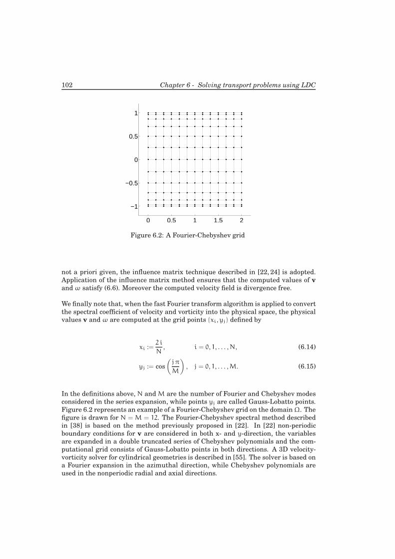
102 Chapter 6 - Solving transport problems using LDC
0 0.5 1 1.5 2
−1
−0.5
0
0.5
1
Figure 6.2: A Fourier-Chebyshev grid
not a priori given, the influence matrix technique described in [22, 24] is adopted.
Application of the influence matrix method ensures that the computed values of v
and ω satisfy (6.6). Moreover the computed velocity field is divergence free.
We finally note that, when the fast Fourier transform algorithm is applied to convert
the spectral coefficient of velocity and vorticity into the physical space, the physical
values v and ω are computed at the grid points (xi, yj) defined by
xi :=2 i
N, i = 0, 1, . . . , N, (6.14)
yj := cos
(
j π
M
)
, j = 0, 1, . . . ,M. (6.15)
In the definitions above, N and M are the number of Fourier and Chebyshev modes
considered in the series expansion, while points yj are called Gauss-Lobatto points.
Figure 6.2 represents an example of a Fourier-Chebyshev grid on the domainΩ. The
figure is drawn for N = M = 12. The Fourier-Chebyshev spectral method described
in [38] is based on the method previously proposed in [22]. In [22] non-periodic
boundary conditions for v are considered in both x- and y-direction, the variables
are expanded in a double truncated series of Chebyshev polynomials and the com-
putational grid consists of Gauss-Lobatto points in both directions. A 3D velocity-
vorticity solver for cylindrical geometries is described in [55]. The solver is based on
a Fourier expansion in the azimuthal direction, while Chebyshev polynomials are
used in the nonperiodic radial and axial directions.
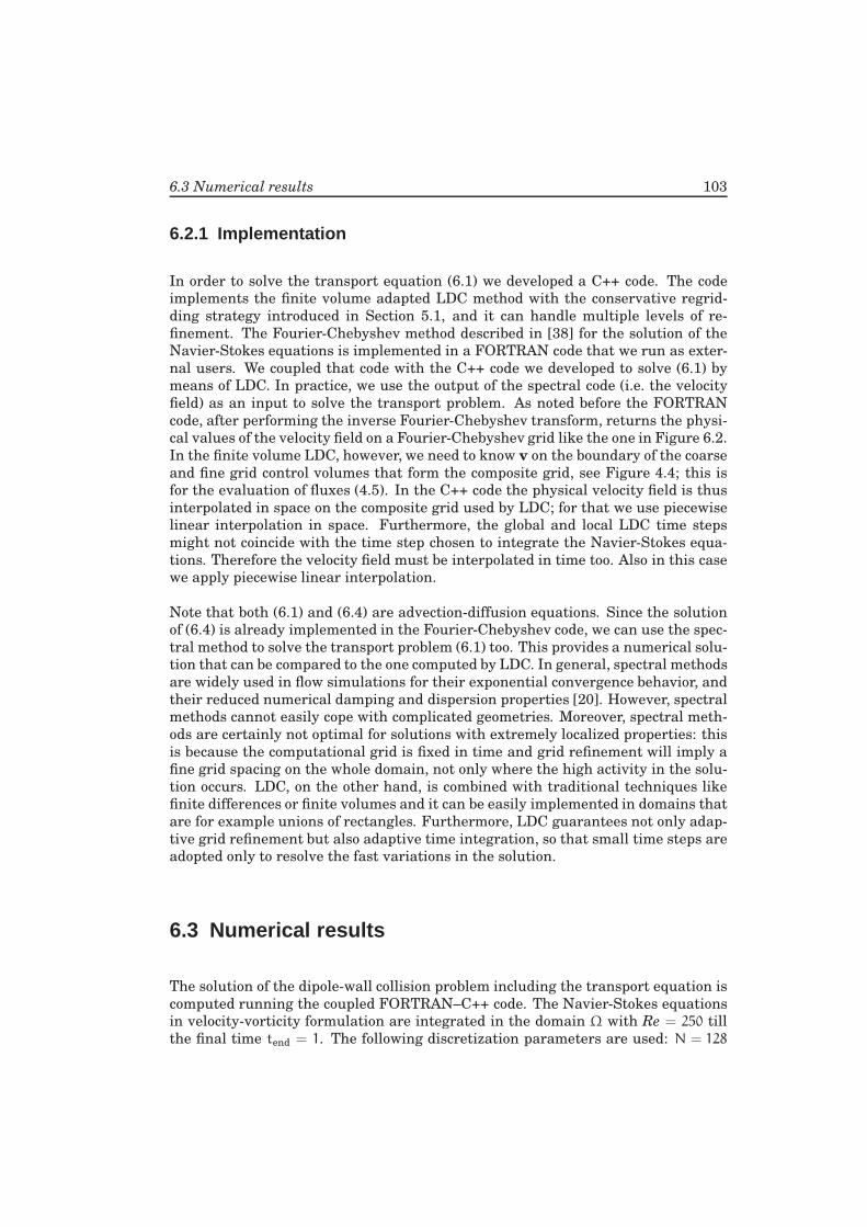
6.3 Numerical results 103
6.2.1 Implementation
In order to solve the transport equation (6.1) we developed a C++ code. The code
implements the finite volume adapted LDC method with the conservative regrid-
ding strategy introduced in Section 5.1, and it can handle multiple levels of re-
finement. The Fourier-Chebyshev method described in [38] for the solution of the
Navier-Stokes equations is implemented in a FORTRAN code that we run as exter-
nal users. We coupled that code with the C++ code we developed to solve (6.1) by
means of LDC. In practice, we use the output of the spectral code (i.e. the velocity
field) as an input to solve the transport problem. As noted before the FORTRAN
code, after performing the inverse Fourier-Chebyshev transform, returns the physi-
cal values of the velocity field on a Fourier-Chebyshev grid like the one in Figure 6.2.
In the finite volume LDC, however, we need to know v on the boundary of the coarse
and fine grid control volumes that form the composite grid, see Figure 4.4; this is
for the evaluation of fluxes (4.5). In the C++ code the physical velocity field is thus
interpolated in space on the composite grid used by LDC; for that we use piecewise
linear interpolation in space. Furthermore, the global and local LDC time steps
might not coincide with the time step chosen to integrate the Navier-Stokes equa-
tions. Therefore the velocity field must be interpolated in time too. Also in this case
we apply piecewise linear interpolation.
Note that both (6.1) and (6.4) are advection-diffusion equations. Since the solution
of (6.4) is already implemented in the Fourier-Chebyshev code, we can use the spec-
tral method to solve the transport problem (6.1) too. This provides a numerical solu-
tion that can be compared to the one computed by LDC. In general, spectral methods
are widely used in flow simulations for their exponential convergence behavior, and
their reduced numerical damping and dispersion properties [20]. However, spectral
methods cannot easily cope with complicated geometries. Moreover, spectral meth-
ods are certainly not optimal for solutions with extremely localized properties: this
is because the computational grid is fixed in time and grid refinement will imply a
fine grid spacing on the whole domain, not only where the high activity in the solu-
tion occurs. LDC, on the other hand, is combined with traditional techniques like
finite differences or finite volumes and it can be easily implemented in domains that
are for example unions of rectangles. Furthermore, LDC guarantees not only adap-
tive grid refinement but also adaptive time integration, so that small time steps are
adopted only to resolve the fast variations in the solution.
6.3 Numerical results
The solution of the dipole-wall collision problem including the transport equation is
computed running the coupled FORTRAN–C++ code. The Navier-Stokes equations
in velocity-vorticity formulation are integrated in the domain Ω with Re = 250 till
the final time tend = 1. The following discretization parameters are used: N = 128
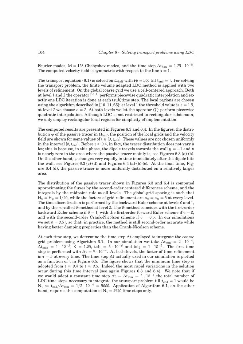
104 Chapter 6 - Solving transport problems using LDC
Fourier modes, M = 128 Chebyshev modes, and the time step ∆tflow = 1.25 · 10−5.
The computed velocity field is symmetric with respect to the line x = 1.
The transport equation (6.1) is solved onΩhalf with Pe = 500 till tend = 1. For solving
the transport problem, the finite volume adapted LDC method is applied with two
levels of refinement. On the global coarse grid we use a cell-centered approach. Both
at level 1 and 2 the operator Ph,H performs piecewise quadratic interpolation and ex-
actly one LDC iteration is done at each (sub)time step. The local regions are chosen
using the algorithm described in [10, 11, 65]; at level 1 the threshold value is ǫ = 1.5,
at level 2 we choose ǫ = 2. At both levels we let the operator Qnx perform piecewise
quadratic interpolation. Although LDC is not restricted to rectangular subdomain,
we only employ rectangular local regions for simplicity of implementation.
The computed results are presented in Figures 6.3 and 6.4. In the figures, the distri-
bution ϕ of the passive tracer inΩhalf, the position of the local grids and the velocity
field are shown for some values of t ∈ [0, tend]. These values are not chosen uniformly
in the interval [0, tend]. Before t ≈ 0.4, in fact, the tracer distribution does not vary a
lot; this is because, in this phase, the dipole travels towards the wall y = −1 and v
is nearly zero in the area where the passive tracer mainly is, see Figures 6.3 (a)-(b).
On the other hand, ϕ changes very rapidly in time immediately after the dipole hits
the wall, see Figures 6.3 (c)-(d) and Figures 6.4 (a)-(b)-(c). At the final time, Fig-
ure 6.4 (d), the passive tracer is more uniformly distributed on a relatively larger
area.
The distribution of the passive tracer shown in Figures 6.3 and 6.4 is computed
approximating the fluxes by the second-order centered differences scheme, and the
integrals by the midpoint rule at all levels. The global grid spacing is such that
Hx = Hy = 1/20, while the factors of grid refinement are σx = σy = 5 at every level.
The time discretization is performed by the backward Euler scheme at levels 0 and 1,
and by the so-called ϑ-method at level 2. The ϑ-method coincides with the first-order
backward Euler scheme if ϑ = 1, with the first-order forward Euler scheme if ϑ = 0,
and with the second-order Crank-Nicolson scheme if ϑ = 0.5. In our simulations
we set ϑ = 0.51, so that, in practice, the method is still second-order accurate while
having better damping properties than the Crank-Nicolson scheme.
At each time step, we determine the time step ∆t employed to integrate the coarse
grid problem using Algorithm 6.1. In our simulation we take ∆tmin = 2 · 10−4,
∆tmax = 1 · 10−3, K = 1.05, tol1 = 6 · 10−6 and tol2 = 1 · 10−5. The first time
step is performed with ∆t = 9 · 10−4. At both levels, the factor of time refinement
is τ = 5 at every time. The time step ∆t actually used in our simulation is plotted
as a function of t in Figure 6.5. The figure shows that the minimum time step is
adopted from t ≈ 0.4 to t ≈ 0.5. Indeed the most rapid variations in the solution
occur during this time interval (see again Figures 6.3 and 6.4). We note that if
we would adopt a constant time step ∆t = ∆tmin = 2 · 10−4 the total number of
LDC time steps necessary to integrate the transport problem till tend = 1 would be
Nt := tend/∆tmin = 1/2 · 10−4 = 5000. Application of Algorithm 6.1, on the other
hand, requires the computation of Nt = 2920 time steps only.
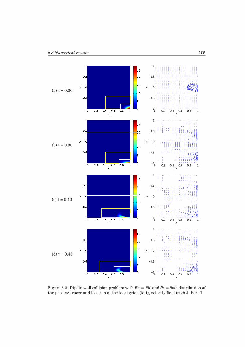
6.3 Numerical results 105
(a) t = 0.00
0 0.2 0.4 0.6 0.8 1−1
−0.5
0
0.5
1
x
y(b) t = 0.30
0 0.2 0.4 0.6 0.8 1−1
−0.5
0
0.5
1
x
y
(c) t = 0.40
0 0.2 0.4 0.6 0.8 1−1
−0.5
0
0.5
1
x
y
(d) t = 0.45
0 0.2 0.4 0.6 0.8 1−1
−0.5
0
0.5
1
x
y
Figure 6.3: Dipole-wall collision problem with Re = 250 and Pe = 500: distribution of
the passive tracer and location of the local grids (left), velocity field (right). Part 1.
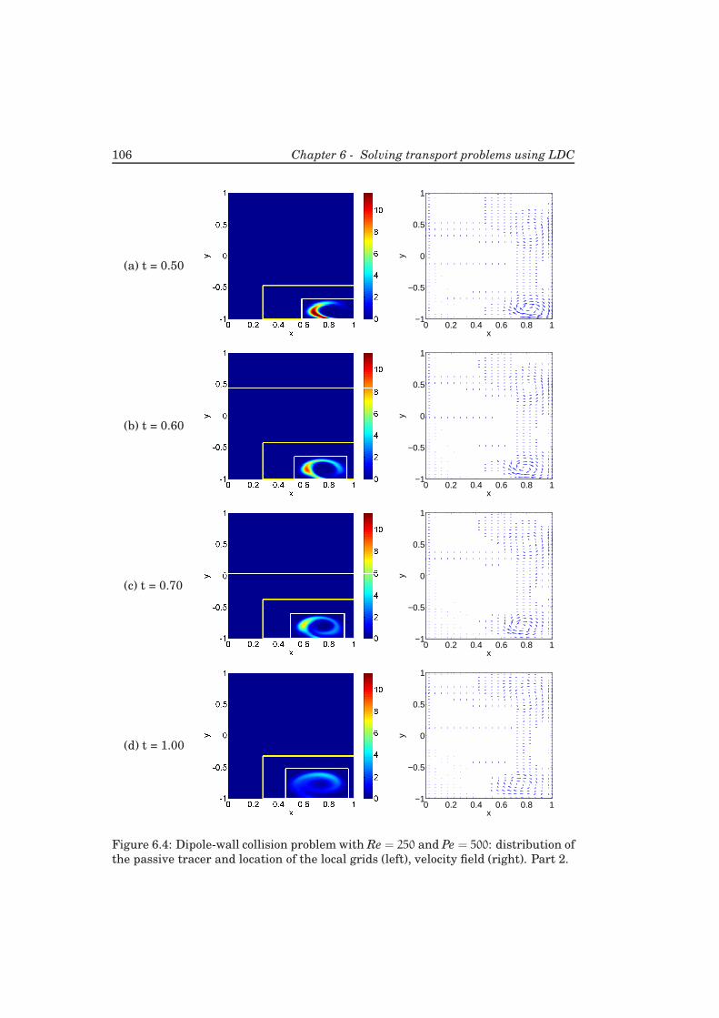
106 Chapter 6 - Solving transport problems using LDC
(a) t = 0.50
0 0.2 0.4 0.6 0.8 1−1
−0.5
0
0.5
1
x
y
(b) t = 0.60
0 0.2 0.4 0.6 0.8 1−1
−0.5
0
0.5
1
x
y
(c) t = 0.70
0 0.2 0.4 0.6 0.8 1−1
−0.5
0
0.5
1
x
y
(d) t = 1.00
0 0.2 0.4 0.6 0.8 1−1
−0.5
0
0.5
1
x
y
Figure 6.4: Dipole-wall collision problem with Re = 250 and Pe = 500: distribution of
the passive tracer and location of the local grids (left), velocity field (right). Part 2.
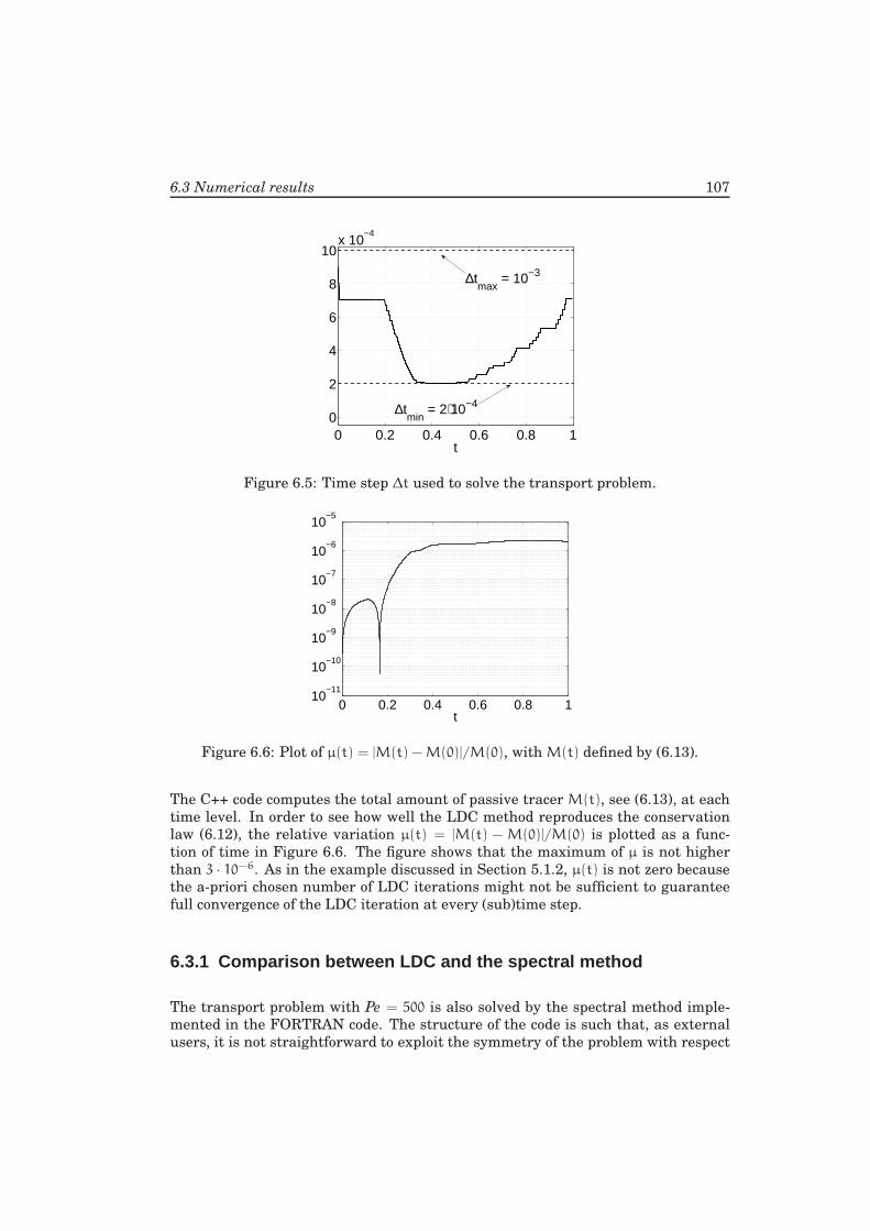
6.3 Numerical results 107
0 0.2 0.4 0.6 0.8 10
2
4
6
8
10x 10
−4
t
∆tmax
= 10−3
∆tmin
= 2⋅10−4
Figure 6.5: Time step ∆t used to solve the transport problem.
0 0.2 0.4 0.6 0.8 110
−11
10−10
10−9
10−8
10−7
10−6
10−5
t
Figure 6.6: Plot of µ(t) = |M(t) −M(0)|/M(0), with M(t) defined by (6.13).
The C++ code computes the total amount of passive tracer M(t), see (6.13), at each
time level. In order to see how well the LDC method reproduces the conservation
law (6.12), the relative variation µ(t) = |M(t) − M(0)|/M(0) is plotted as a func-
tion of time in Figure 6.6. The figure shows that the maximum of µ is not higher
than 3 · 10−6. As in the example discussed in Section 5.1.2, µ(t) is not zero because
the a-priori chosen number of LDC iterations might not be sufficient to guarantee
full convergence of the LDC iteration at every (sub)time step.
6.3.1 Comparison between LDC and the spectral method
The transport problem with Pe = 500 is also solved by the spectral method imple-
mented in the FORTRAN code. The structure of the code is such that, as external
users, it is not straightforward to exploit the symmetry of the problem with respect
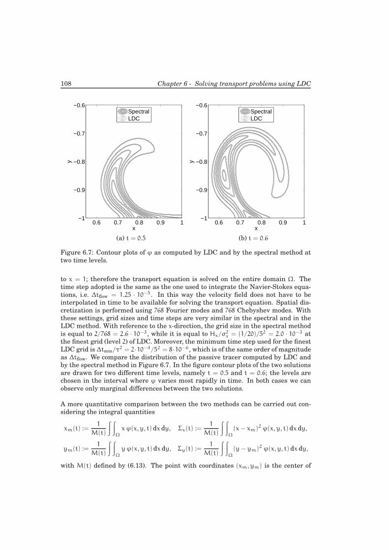
108 Chapter 6 - Solving transport problems using LDC
x
y
0.6 0.7 0.8 0.9 1−1
−0.9
−0.8
−0.7
−0.6SpectralLDC
x
y
0.6 0.7 0.8 0.9 1−1
−0.9
−0.8
−0.7
−0.6SpectralLDC
(a) t = 0.5 (b) t = 0.6
Figure 6.7: Contour plots of ϕ as computed by LDC and by the spectral method at
two time levels.
to x = 1; therefore the transport equation is solved on the entire domain Ω. The
time step adopted is the same as the one used to integrate the Navier-Stokes equa-
tions, i.e. ∆tflow = 1.25 · 10−5. In this way the velocity field does not have to be
interpolated in time to be available for solving the transport equation. Spatial dis-
cretization is performed using 768 Fourier modes and 768 Chebyshev modes. With
these settings, grid sizes and time steps are very similar in the spectral and in the
LDC method. With reference to the x-direction, the grid size in the spectral method
is equal to 2/768 = 2.6 · 10−3, while it is equal to Hx/σ2x = (1/20)/52 = 2.0 · 10−3 at
the finest grid (level 2) of LDC. Moreover, the minimum time step used for the finest
LDC grid is ∆tmin/τ2 = 2·10−4/52 = 8·10−6, which is of the same order of magnitude
as ∆tflow. We compare the distribution of the passive tracer computed by LDC and
by the spectral method in Figure 6.7. In the figure contour plots of the two solutions
are drawn for two different time levels, namely t = 0.5 and t = 0.6; the levels are
chosen in the interval where ϕ varies most rapidly in time. In both cases we can
observe only marginal differences between the two solutions.
A more quantitative comparison between the two methods can be carried out con-
sidering the integral quantities
xm(t) :=1
M(t)
∫ ∫
Ω
xϕ(x, y, t) dx dy, Σx(t) :=1
M(t)
∫ ∫
Ω
(x− xm)2ϕ(x, y, t) dx dy,
ym(t) :=1
M(t)
∫ ∫
Ω
yϕ(x, y, t) dx dy, Σy(t) :=1
M(t)
∫ ∫
Ω
(y− ym)2ϕ(x, y, t) dx dy,
with M(t) defined by (6.13). The point with coordinates (xm, ym) is the center of
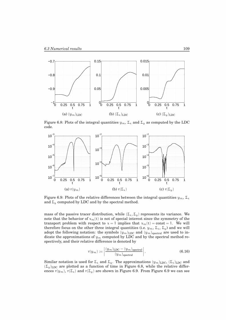
6.3 Numerical results 109
0 0.25 0.5 0.75 1−1
−0.9
−0.8
−0.7
t0 0.25 0.5 0.75 1
0
0.05
0.1
0.15
t0 0.25 0.5 0.75 1
0
0.005
0.01
0.015
t
(a) (ym)LDC (b) (Σx)LDC (c) (Σy)LDC
Figure 6.8: Plots of the integral quantities ym, Σx and Σy as computed by the LDC
code.
0 0.25 0.5 0.75 110
−7
10−6
10−5
10−4
10−3
t0 0.25 0.5 0.75 1
10−5
10−4
10−3
10−2
t0 0.25 0.5 0.75 1
10−6
10−5
10−4
10−3
10−2
t
(a) r(ym) (b) r(Σx) (c) r(Σy)
Figure 6.9: Plots of the relative differences between the integral quantities ym, Σx
and Σy computed by LDC and by the spectral method.
mass of the passive tracer distribution, while (Σx, Σy) represents its variance. We
note that the behavior of xm(t) is not of special interest since the symmetry of the
transport problem with respect to x = 1 implies that xm(t) = const = 1. We will
therefore focus on the other three integral quantities (i.e. ym, Σx, Σy) and we will
adopt the following notation: the symbols (ym)LDC and (ym)spectral are used to in-
dicate the approximations of ym computed by LDC and by the spectral method re-
spectively, and their relative difference is denoted by
r(ym) :=
∣
∣
∣
∣
(ym)LDC − (ym)spectral
(ym)spectral
∣
∣
∣
∣
. (6.16)
Similar notation is used for Σx and Σy. The approximations (ym)LDC, (Σx)LDC and
(Σy)LDC are plotted as a function of time in Figure 6.8, while the relative differ-
ences r(ym), r(Σx) and r(Σy) are shown in Figure 6.9. From Figure 6.9 we can see
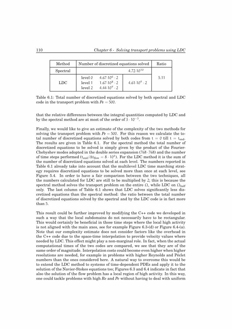
110 Chapter 6 - Solving transport problems using LDC
Method Number of discretized equations solved Ratio
Spectral 4.72·1010
level 0 4.67·106 · 2 5.11
LDC level 1 1.67·108 · 2 4.61·109 · 2level 2 4.44·109 · 2
Table 6.1: Total number of discretized equations solved by both spectral and LDC
code in the transport problem with Pe = 500.
that the relative differences between the integral quantities computed by LDC and
by the spectral method are at most of the order of 3 · 10−3.
Finally, we would like to give an estimate of the complexity of the two methods for
solving the transport problem with Pe = 500. For this reason we calculate the to-
tal number of discretized equations solved by both codes from t = 0 till t = tend.
The results are given in Table 6.1. For the spectral method the total number of
discretized equations to be solved is simply given by the product of the Fourier-
Chebyshev modes adopted in the double series expansion (768 · 768) and the number
of time steps performed (tend/∆tflow = 8 · 104). For the LDC method it is the sum of
the number of discretized equations solved at each level. The numbers reported in
Table 6.1 already take into account that the multilevel LDC time marching strat-
egy requires discretized equations to be solved more than once at each level, see
Figure 5.4. In order to have a fair comparison between the two techniques, all
the numbers calculated for LDC are still to be multiplied by 2; this is because the
spectral method solves the transport problem on the entire Ω, while LDC on Ωhalf
only. The last column of Table 6.1 shows that LDC solves significantly less dis-
cretized equations than the spectral method: the ratio between the total number
of discretized equations solved by the spectral and by the LDC code is in fact more
than 5.
This result could be further improved by modifying the C++ code we developed in
such a way that the local subdomains do not necessarily have to be rectangular.
This would certainly be beneficial in those time steps where the local high activity
is not aligned with the main axes, see for example Figure 6.3-(d) or Figure 6.4-(a).
Note that our complexity estimate does not consider factors like the overhead in
the C++ code due to the space-time interpolation to provide velocity values where
needed by LDC. This effect might play a non-marginal role. In fact, when the actual
computational times of the two codes are compared, we see that they are of the
same order of magnitude. Interpolation costs could become even higher when higher
resolutions are needed, for example in problems with higher Reynolds and Peclet
numbers than the ones considered here. A natural way to overcome this would be
to extend the LDC method to systems of time-dependent PDEs and apply it to the
solution of the Navier-Stokes equations too; Figures 6.3 and 6.4 indicate in fact that
also the solution of the flow problem has a local region of high activity. In this way,
one could tackle problems with high Re and Pe without having to deal with uniform

6.3 Numerical results 111
fine meshes and time steps like required by spectral methods; using LDC, one can
adopt relatively small grid sizes and time steps to resolve the local high activity only.
In conclusion, the example presented in this section suggests that the LDC method
for parabolic partial differential equations we developed and analyzed in this thesis
is a valid alternative to spectral methods for the solution of transport problems with
highly localized properties.

Chapter 7
Conclusions andrecommendations
In this thesis we present, analyze and implement a new static-regridding technique
for parabolic partial differential equations: Local Defect Correction. The method
generalizes the LDC technique initially introduced for the efficient solution of ellip-
tic problems with highly localized properties. In particular, the original idea of local
defect correction is extended in the sense that the defect term is used to correct the
error of the global coarse grid approximation not only due to the spatial dicretiza-
tion, but also to the time discretization. This can be achieved by solving the local
problem not only with a finer grid size, but also with a smaller time step than the
one adopted globally. One of the main advantages of LDC is that one may work
with uniform structured grids and uniform grid solvers only. In comparison with
dynamic-regridding methods, LDC requires very little tuning of user-specified pa-
rameters; basically, just one parameter has to be set in LDC: this is for the adaptive
choice of the local domain at each time level.
We discuss some properties of the LDC algorithm for parabolic problems. In par-
ticular, we show that coarse and fine grid solution coincide at the common points
between the two grids, and we derive the system of discretized equations that the
composite grid solution satisfies. The LDC method is tested on some concrete ex-
amples, that illustrate its accuracy, efficiency and robustness. A direction for future
research is to provide error bounds for the LDC composite grid solution at a generic
time level. The error estimates should take into account all the approximations in-
troduced by the numerical method: space and time discretization on the global and
on the local grid, space and time interpolation to provide artificial boundary for the
local problem, space interpolation to provide initial values in all the points of the
new composite grid during regridding.
114 Chapter 7 - Conclusions and recommendations
The LDC method produces a composite grid solution at the new time level combin-
ing a global and a local approximation iteratively. The convergence behavior of the
LDC algorithm is studied in detail in this thesis: a general expression for the itera-
tion matrix of the method is derived, and the properties of the iteration matrix are
studied both analytically and by means of numerical experiments. The results of the
analysis illustrate how the coarse grid discretization parameters (grid size and time
step) and the choice of the so-called safety region influence the convergence rate of
the LDC algorithm. In general, we observe that LDC converges for any choice of the
discretization parameters and that iteration errors are reduced by several orders of
magnitude at every iteration.
In this thesis we also propose a finite volume adapted LDC algorithm for time-
dependent problems that yields discrete conservation on the composite grid. This
result can be achieved by writing the defect term in such a way that a balance
of fine and coarse grid fluxes is guaranteed across the interface between the two
grids at each time level. The method can handle the fact that time integration on
the local grid is performed with a smaller time step than the one adopted globally.
The finite volume adapted LDC algorithm is successfully tested in some numerical
experiments, and then extended to incorporate a conservative regridding strategy
and multiple levels of refinement. Further improvements of the method might be
the implementation of general Runge-Kutta schemes for time integration, or the
design of a tailored strategy for detecting the local high activity at each (sub)time
level.
The multilevel conservative LDC algorithm is finally applied to solve transport
problems in transient flow fields. With reference to a dipole-wall collision prob-
lem, the results computed by LDC are compared to the solution computed by a
Chebyshev-Fourier spectral method. The two techniques give very similar solu-
tions when similar grid spacing and time steps are adopted; yet, LDC requires the
solution of a smaller number of discretized equations. As mentioned before, the ef-
ficiency of LDC could be further improved by allowing the local subdomains to have
a more general shape than rectangles, for example union of rectangles. The results
presented and, in general, the attractive properties of LDC make future research
on local defect correction methods worthwhile. Interesting topics would certainly
be the solution of systems of time-dependent partial differential equations and the
application of LDC to more complex transport and flow problems.
Bibliography
[1] M. J. H. Anthonissen. Local defect correction techniques: analysis and appli-
cation to combustion. PhD thesis, Eindhoven University of Technology, Eind-
hoven, 2001.
[2] M. J. H. Anthonissen. Local defect correction techniques applied to a combus-
tion problem. In R. Kornhuber, R. Hoppe, J. Periaux, O. Pironneau, O. Widlund,
and J. Xu, editors, Domain Decomposition Methods in Science and Engineer-
ing, Lecture Notes in Computational Science and Engineering, pages 185–192,
Berlin, Heidelberg, New York, 2005. Springer.
[3] M. J. H. Anthonissen, B. A. V. Bennett, and M. D. Smooke. An adaptive mul-
tilevel local defect correction technique with application to combustion. Com-
bustion Theory and Modelling, 9:273–299, 2005.
[4] M. J. H. Anthonissen, R. M. M. Mattheij, and J. H. M. ten Thije Boonkkamp.
Convergence analysis of the local defect correction method for diffusion equa-
tions. Numerische Mathematik, 95:401–425, 2003.
[5] M. J. H. Anthonissen and R. Minero. Conditions for one-step convergence of
the local defect correction method for elliptic problems. Technical Report CASA
05-39, Eindhoven University of Technology, Eindhoven, November 2005.
[6] M. J. H. Anthonissen, B. van ’t Hof, and A. A. Reusken. A finite volume scheme
for solving elliptic boundary value problems on composite grids. Computing,
61:285–305, 1998.
[7] M. Barad and P. Colella. A fourth-order accurate local refinement method for
Poisson’s equation. Journal of Computational Physics, 209:1–18, 2005.
[8] G. Beckett, J. A. Mackenzie, A. Ramage, and D. M. Sloan. On the numerical
solution of one-dimensional PDEs using adaptive methods based on equidistri-
bution. Journal of Computational Physics, 167:372–392, 2001.
[9] G. Beckett, J. A. Mackenzie, A. Ramage, and D. M. Sloan. Computational solu-
tion of two-dimensional unsteady PDEs using moving mesh methods. Journal
of Computational Physics, 182:478–495, 2002.
116 Bibliography
[10] B. A. V. Bennett and M. D. Smooke. Local rectangular refinement with ap-
plication to axisymmetric laminar flames. Combustion Theory and Modelling,
2:221–258, 1998.
[11] B. A. V. Bennett and M. D. Smooke. Local rectangular refinement with applica-
tion to nonreacting and reacting fluid flow problems. Journal of Computational
Physics, 151:684–727, 1999.
[12] M. J. Berger and P. Colella. Local adaptive mesh refinement for shock hydro-
dynamics. Journal of Computational Physics, 82:64–84, 1989.
[13] M. J. Berger and R. J. Leveque. Adaptive mesh refinement using wave-
propagation algorithms for hyperbolic systems. SIAM Journal on Numerical
Analysis, 35:2298–2316, 1998.
[14] M. J. Berger and J. Oliger. Adaptive mesh refinement for hyperbolic partial
differential equations. Journal of Computational Physics, 53:484–512, 1984.
[15] L. K. Bieniasz. Use of dynamically adaptive grid techniques for the solu-
tion of electrochemical kinetic equations: Part 5. A finite-difference, adaptive
space/time grid strategy based on a patch-type local uniform spatial grid re-
finement, for kinetic models in one-dimensional space geometry. Journal of
Electroanalytical Chemistry, 481:115–133, 2000.
[16] J. G. Blom and J. G. Verwer. VLUGR3: a vectorizable adaptive grid solver for
PDEs in 3D, part I: algorithmic aspects and applications. Applied Numerical
Mathematics, 16:129–156, 1994.
[17] F. Bramkamp, P. Lamby, and S. Muller. An adaptive multiscale finite volume
solver for unsteady and steady state flow computations. Journal of Computa-
tional Physics, 197:460–490, 2004.
[18] A. Brandt. Multi-level adaptive solutions to boundary value problems. Mathe-
matics of Computation, 31:333–390, 1977.
[19] W. L. Briggs, V. E. Henson, and S. F. McCormick. A multigrid tutorial. SIAM,
Philadelphia, 2nd edition, 2000.
[20] C. Canuto, M. Y. Hussaini, A. Quarteroni, and T. A. Zang. Spectral Methods in
Fluid Dynamics. Springer-Verlag, 1988.
[21] C. Carstensen, R. D. Lazarov, and S. Tomov. Explicit and averaging a posteriori
error estimates for adaptive finite volume methods. SIAM Journal on Numer-
ical Analysis, 42:2496–2521, 2005.
[22] H. J. H. Clercx. A spectral solver for the Navier-Stokes equations in the
velocity-vorticity formulation for flows with two nonperiodic directions. Jour-
nal of Computational Physics, 137:186–211, 1997.
[23] H. J. H. Clercx and C. H. Bruneau. The normal and oblique collision of a dipole
with a no-slip boundary. Computers and Fluids, 35:245–279, 2006.
Bibliography 117
[24] O. Daube. Resolution of the 2D Navier-Stokes equations in velocity-vorticity
form by means of an influence matrix technique. Journal of Computational
Physics, 103:402–414, 1992.
[25] C. Dawson and R. Kirby. High resolution schemes for conservation laws with
locally varying time steps. SIAM Journal on Scientific Computing, 22:2256–
2281, 2001.
[26] P. E. Dimotakis. Turbulent mixing. Annual Review of Fluid Mechanics, 37:329–
356, 2005.
[27] P. J. J. Ferket. Coupling of a global coarse discretization and local fine dis-
cretizations. In W. Hackbusch and G. Wittum, editors, Numerical Treatment
of Coupled Systems, volume 51 of Notes on Numerical Fluid Mechanics, pages
47–58, Braunschweig, 1995. Vieweg.
[28] P. J. J. Ferket. Solving boundary value problems on composite grids with an
application to combustion. PhD thesis, Eindhoven University of Technology,
Eindhoven, 1996.
[29] P. J. J. Ferket and A. A. Reusken. Further analysis of the local defect correction
method. Computing, 56:117–139, 1996.
[30] P. J. J. Ferket and A. A. Reusken. A finite difference discretization method on
composite grids. Computing, 56:343–369, 1996.
[31] J. E. Flaherty, R. M. Loy, M. S. Shephard, B. K. Skymanski, J. D. Teresco,
and L. H. Ziantz. Adaptive local refinement with octree load balancing for the
parallel solution of three-dimensional conservation laws. Journal of Parallel
and Distributed Computing, 47:139–152, 1997.
[32] M. Graziadei. Using local defect correction for laminar flame simulation. PhD
thesis, Eindhoven University of Technology, Eindhoven, 2004.
[33] M. Graziadei, R. M. M. Mattheij, and J. H. M. ten Thije Boonkkamp. Local de-
fect correction with slanting grids. Numerical Methods for Partial Differential
Equations, 20:1–17, 2003.
[34] W. Hackbusch. Local defect correction and domain decomposition techniques.
In K. Bohmer and H. J. Stetter, editors, Defect Correction Methods. Theory
and Applications, Computing, Suppl. 5, pages 89–113, Wien, New York, 1984.
Springer.
[35] W. Huang. Practical aspects of formulation and solution of moving mesh partial
differential equations. Journal of Computational Physics, 171:753–775, 2001.
[36] W. Huang, Y. Ren, and R. D. Russell. Moving mesh partial differential equa-
tions (MMPDES) based on the equidistribution principle. SIAM Journal on
Numerical Analysis, 31:709–730, 1994.
118 Bibliography
[37] W. Huang and R. D. Russell. Moving mesh strategy based on a gradient flow
equation for two-dimensional problems. SIAM Journal on Scientific Comput-
ing, 20:998–1015, 1999.
[38] W. Kramer. Dispersion of passive tracers in two-dimensional bounded flows.
PhD thesis, Eindhoven University of Technology, Eindhoven, to appear in 2006.
[39] R. D. Lazarov, I. D. Mishev, and P. S. Vassilevski. Finite volume methods with
local refinement for convection-diffusion problems. Computing, 53:33–57, 1994.
[40] R. D. Lazarov and S. Tomov. A posteriori error estimates for finite volume
element approximations of convection-diffusion-reaction equations. Computa-
tional Geosciences, 6:483–503, 2002.
[41] S. McCormick. Fast adaptive composite grid (FAC) methods: Theory for the
variational case. In K. Bohmer and H. J. Stetter, editors, Defect Correction
Methods. Theory and Applications, Computing, Suppl. 5, pages 115–121, Wien,
New York, 1984. Springer.
[42] S. F. McCormick and J. Thomas. The fast adaptive composite grid (FAC)
method for elliptic equations. Mathematics of Computation, 46:439–456, 1986.
[43] R. Minero, M. J. H. Anthonissen, and R. M. M. Mattheij. Local defect correction
for time-dependent partial differential equations. In Proceedings of the 16th
International Conference on Domain Decomposition Methods, 2005. Available
online at http://cims.nyu.edu/dd16/proceedings.html.
[44] R. Minero, M. J. H. Anthonissen, and R. M. M. Mattheij. A local defect cor-
rection technique for time-dependent problems. Numerical Methods for Partial
Differential Equations, 22:128–144, 2006.
[45] R. Minero, M. J. H. Anthonissen, and R. M. M. Mattheij. Solving parabolic
problems using local defect correction in combination with the finite volume
method. Numerical Methods for Partial Differential Equations, 2006. In press.
[46] R. Minero, H. G. ter Morsche, and M. J. H. Anthonissen. Convergence prop-
erties of the local defect correction method for parabolic problems. Technical
Report CASA 05-40, Eindhoven University of Technology, Eindhoven, Novem-
ber 2005. Submitted for publication.
[47] V. Nefedov and R. M. M. Mattheij. Local defect correction with different grid
types. Numerical Methods for Partial Differential Equations, 18:454–468, 2002.
[48] D. Norman. Introduction to Linear Algebra for Science and Engineering.
Addison-Wesley Publishers Limited, 1995.
[49] P. Orlandi. Vortex dipole rebound from a wall. Physics of Fluids A, 2:1429–
1436, 1990.
[50] T. Plewa and E. Muller. AMRA: an adaptive mesh refinement hydrodynamic
code for astrophysics. Computer Physics Communications, 138:101–127, 2001.
Bibliography 119
[51] O. Roussel, K. Schneider, A. Tsigulin, and H. Bockhorn. A conservative fully
adaptive multiresolution algorithm for parabolic PDEs. Journal of Computa-
tional Physics, 188:493–523, 2003.
[52] B. Sawford. Turbulent relative dispersion. Annual Review of Fluid Mechanics,
33:289–317, 2001.
[53] I. E. M. Severens, M. J. H. Anthonissen, R. M. M. Mattheij, and J. M. L.
Maubach. Application of the local defect correction method in discrete element
method simulations. Technical Report CASA 04-17, Eindhoven University of
Technology, Eindhoven, August 2004.
[54] M. Sizov, M. J. H. Anthonissen, and R. M. M. Mattheij. Analysis of local defect
correction and high-order compact finite differences. Numerical Methods for
Partial Differential Equations, 22:815–830, 2006.
[55] M. F. M. Speetjens and H. J. H. Clercx. A spectral solver in the velocity-vorticity
formulation for low Reynolds number flows in 3D cylindrical cavities. Interna-
tional Journal of Computational Fluid Dynamics, 19:191–209, 2005.
[56] M. F. M. Speetjens, H. J. H. Clercx, and G. J. F. van Heijst. A numerical and
experimental study on advection in three-dimensional Stokes flows. Journal of
Fluid Mechanics, 514:77–105, 2004.
[57] Z. Tan, Z. Zhang, Y. Huang, and T. Tang. Moving mesh methods with locally
varying time steps. Journal of Computational Physics, 200:347–367, 2004.
[58] H. Tang and T. Tang. Adaptive mesh methods for one- and two-dimensional
hyperbolic conservation laws. SIAM Journal on Numerical Analysis, 41:487–
515, 2003.
[59] C. R. Traas, H. G. ter Morsche, and R. M. J. van Damme. Splines en Wavelets.
Epsilon Uitgaven, Utrecht, 2000. In Dutch.
[60] R. A. Trompert. Local uniform grid refinement and systems of coupled partial
differential equations. Applied Numerical Mathematics, 13:251–270, 1993.
[61] R. A. Trompert. Local-uniform-grid refinement and transport in heterogeneous
porous media. Advances in Water Resources, 16:293–304, 1993.
[62] R. A. Trompert. Local Uniform Grid refinement for Time-Dependent Partial
Differential Equations. PhD thesis, University of Amsterdam, Amsterdam,
1994.
[63] R. A. Trompert and J. G. Verwer. Analysis of the implicit Euler local uniform
grid refinement method. SIAM Journal on Scientific Computing, 14:259–278,
1993.
[64] R. A. Trompert and J. G. Verwer. Runge-Kutta methods and local uniform grid
refinement. Mathematics of Computation, 60:591–616, 1993.
120 Bibliography
[65] B. A. Valdati (Bennett). Solution-adaptive gridding methods with application
to combustion problems. PhD thesis, Yale University, New Haven, CT, 1997.
[66] J. U. Wappler. Die lokale Defektkorrekturmethode zur adaptiven
Diskretisierung elliptischer Differentialgleichungen mit finiten Elementen.
PhD thesis, Christian-Albrechts-Universitat, Kiel, 1999. In German.
[67] Z. Warhaft. Passive scalars in turbulent flows. Annual Review of Fluid Me-
chanics, 32:203–240, 2000.
[68] P. A. Zegeling and H. P. Kok. Adaptive moving mesh computations for
reaction-diffusion systems. Journal of Computational and Applied Mathemat-
ics, 168:519–528, 2004.
Index
ABCN scheme, 101
Adams-Bashforth scheme, 101
AMR, 2, 3
asymptotic equivalence, 42
backward Euler, 11, 34, 65
balance of fluxes, 76–77
across the interface, 6, 59
boundary conditions
artificial, 4, 12–13, 65
different types, 10, 60, 66
flow problem, 99
in spectral method, 101
C++ code, 103, 110
cell-centered approach, 78
Chebyshev polynomials, 101, 102
complexity, 25, 81, 110
conservation in LDC
during regridding, 85–89
numerical examples, 79–84, 91–93
system of discrete cons. laws, 77
control volume, 61
convergence of LDC
1D Poisson’s equation, 46
1D convection-diffusion problem, 51
1D diffusion problem, 47, 49
2D Poisson’s equation, 6, 31, 55
2D convection-diffusion problem, 56
2D diffusion problem, 53
in one iteration, 46
Crank-Nicolson scheme, 101, 104
defect, 14, 67
approximation, 68–71
differential formulation, 60
diffusion coefficient, 60
dipole, 99
Direct Numerical Simulations (DNS),
1, 97
divergence free, 60, 102
dynamic-regridding methods, 2
explicit time integration in LDC, 21
FAC, 4
factor of time refinement, 64
factors of grid refinement, 63
fast Fourier transform (FFT), 101
flux, 60
FORTRAN code, 103, 107
Fourier transform, 41
Fourier-Chebyshev
grid, 102–103
inverse transform, 103
Gauss-Lobatto points, 102
grid
composite, 4, 9, 63
global coarse, 10, 34, 61
local fine, 10, 63
grid function, 11, 61
heat equation
one-dimensional, 34, 38, 49
two-dimensional, 53
homogeneous system, 76
implicit Euler, see backward Euler
influence matrix, 102
122 Index
initial values for LDC time step, 21,
65, 85–90
integral formulation, 60, 91
integral quantities, 108–110
integrated flux, 62
interface, 12
interpolation
compute velocity field, 103
local boundary conditions, 4, 13, 65
piecewise linear, 23, 27, 80, 84
piecewise quadratic, 104
regridding, 19, 88
iteration error, 32
iteration matrix, 33
kinetic energy of a flow, 100
Lanczos tau method, 101
LDC algorithm
elliptic problems, 4
finite volume adapted, 71
finite volume adapted with regrid-
ding, 89
multiple levels of refinement, 93
parabolic problems, 20
LDC convergence, see convergence of
LDC
LDC iteration, 4, 14
fixed point, 17
stopping criterion, 21
local discretization error, see defect
local region
choice of, 19, 63
circular shape, 6
slantwise direction, 6
LUGR, 3, 9
vs. LDC, 26–29
midpoint rule, 62
in numerical experiments, 80, 82,
91, 104
regridding, 88–89
MLAT, 4, 5
MMPDE, 2
moving-grid methods, 2–3
Navier-Stokes equations, 98–99
non-uniform convergence, 43–44
partition of coarse grid points, 12
Peclet number, 98
Poisson summation formula, 41
Poisson’s equation, 5, 6, 31, 46
for the velocity field, 101
regridding strategy, 18–19, 85–89
replacement
of coarse grid solution locally, 22
symbol, 89
residual, 39
restriction operator, 14
Reynolds number, 99
Runge-Kutta schemes
in LDC, 21, 65, 114
in spectral method, 101
safety region, 14–15, 46–57
separation of variables, 39
source term, 10, 60
spectral method, 101
vs. LDC, 103, 107–111
spectral radius, 33
static-regridding methods, 2
symmetric diagonalization theorem, 36
Taylor expansions, 39
ϑ-method, 104
time marching, 8, 94
uniform convergence, 44–45
uniform grid, 3, 113
coarse, see grid, global coarse
fine, see grid, local fine
uniform grid solver, 3, 18, 113
vs. LDC, 22–26, 79–81
velocity-vorticity formulation, see Navier-
Stokes equations
vertex-centered approach, 61
vorticity, 98
Summary
The solutions of partial differential equations (PDEs) describing physical phenom-
ena are often characterized by local regions of high activity, i.e., regions where spa-
tial gradients are quite large compared to those in the rest of the domain, where
the solution presents a relatively smooth behavior. Examples are encountered in
many application areas; one of them is the transport of passive tracers in turbu-
lent flow fields. A passive tracer is a diffusive contaminant in a fluid flow that is
present in such low concentration that it does not influence the dynamics of the
flow. A few examples of passive tracer transport from everyday life are the exhaust
gases from chimneys, smoke from a cigarette, dust particles spread by the wind, etc.
Understanding the influence of the main flow on the tracer material is crucial in
many engineering applications, such as mixing in chemical reactors or transport of
fly ashes in burners. Knowledge of the passive tracer behavior is also of fundamen-
tal importance in environmental sciences for studying dispersion of pollutants (e.g.
chemical species, radioactive components) in the atmosphere or in the oceans. Since
filaments of tracer material are often concentrated only in a very limited part of
the computational domain, an efficient numerical solution of this type of problems
requires the usage of adaptive grid techniques. In adaptive grid methods, a fine grid
spacing and a relatively small time step are adopted only where the relatively large
variations occur, so that the computational effort and the memory requirements are
minimized.
This thesis focuses on a new adaptive grid method for efficiently solving parabolic
PDEs characterized by highly localized properties: Local Defect Correction (LDC).
In LDC the PDE is integrated on a global uniform coarse grid and on a local uniform
fine grid; the latter is adaptively placed at each time level where the high activity
in the solution occurs. At each time step, global and local solution are iteratively
combined to ultimately produce a solution on the composite grid, union of global
and local grid. In particular, the global approximation provides artificial boundary
conditions for the local fine grid problem, while the local approximation is used to
estimate the coarse grid local discretization error (or defect) and then to improve
the solution globally by means of a defect correction. In the algorithm we propose,
the local problem is solved not only with a smaller grid size, but also with a smaller
time step than the one used for the global problem. In this way the local solution
124 Summary
corrects the error in the global approximation due not only to spatial discretization,
but also to temporal discretization. When the LDC iteration has come to a fixed
point, it can be proved that the global and the local solution at the new time level
coincide at the common points between the two grids. The method described in this
thesis extends the LDC technique that was initially introduced in the literature for
solving elliptic PDEs. The new LDC algorithm is tested in some concrete examples
that illustrate its accuracy, efficiency and robustness.
LDC is an iterative process that can be used for practical applications only if it
converges sufficiently fast. In this thesis the convergence properties of the LDC
method for time-dependent problems are studied in detail, both analytically and
by means of numerical experiments. For both one- and two-dimensional problems
we investigate the dependency of the LDC convergence rate on the discretization
parameters (grid size and time step) for the coarse grid problem. In general, it is
observed that LDC converges for any choice of the discretization parameters and
that iteration errors are reduced by several orders of magnitude at every iteration.
When the coarse and the fine grid problem are discretized applying the finite volume
method, special care is needed to guarantee that a discrete conservation property
holds for the LDC solution on the composite grid. In fact, if no special precau-
tions are taken, the standard LDC method for time-dependent problems is such
that fluxes across the interface between global and local grid are not necessarily
in balance. In this thesis we propose a finite volume adapted LDC algorithm for
parabolic PDEs. In this algorithm the defect term is adapted in such a way that, at
each time step, fluxes across the interface between global and local grid are in bal-
ance at convergence of the LDC iteration. The finite volume adapted LDC algorithm
is then extended to include a conservative regridding strategy. The strategy guaran-
tees that the composite grid solution satisfies a discrete conservation law also when
the local region is moved in time to follow the behavior of the solution.
The LDC technique is not restricted to one level of refinement. In this thesis a mul-
tilevel LDC method for time-dependent problems is introduced. The time marching
strategy is such that time integration at the finer levels can be performed with
smaller time steps. Finally, the new, fast converging, conservative and multilevel
LDC algorithm is applied to solve a transport problem with highly localized proper-
ties. In particular, we test the LDC method on a dipole-wall collision problem. The
problem is solved both by LDC and by a Chebyshev-Fourier spectral method. When
the two numerical solutions are compared, we see that the two methods yield very
similar results. LDC, however, is specifically meant for solving problems whose so-
lutions exhibit local regions of high activity, and for this reason it turns out to be a
less complex algorithm than the Chebyshev-Fourier spectral method.
Samenvatting
Oplossingen van partiele differentiaalvergelijkingen (PDV’en) die fysische verschijn-
selen beschrijven worden vaak gekenmerkt door lokale gebieden met hoge activi-
teit. Dit zijn gebieden waar de plaatsafgeleiden groot zijn in verhouding tot de gra-
dienten in de rest van het domein waar de oplossing relatief glad is. Er zijn tal van
voorbeelden te vinden in verschillende toepassingsgebieden zoals bijvoorbeeld het
transport van merkstof in turbulente stromingen. Een merkstof is een verontreini-
ging die zich in een vloeistofstroming verspreidt en in dusdanig lage concentraties
aanwezig is dat de dynamica van de stroming niet wordt beınvloed. Alledaagse voor-
beelden van merkstoffen zijn de gassen uit een schoorsteen of uitlaat, rook van een
sigaret en door de wind getransporteerde stofdeeltjes. Het begrijpen van de invloed
van de hoofdstroming op de merkstofdeeltjes is belangrijk voor tal van technische
toepassingen zoals het mixen in een chemische reactor of het transport van vliegas
in een brander. Kennis van het gedrag van een merkstof is ook van fundamenteel
belang in milieustudies naar de verspreiding van vervuiling (zoals chemische stof-
fen of radioactieve componenten) in de atmosfeer of oceaan. Omdat filamenten van
merkstofmateriaal vaak geconcentreerd zijn in een klein deel van het rekendomein
zijn adaptieve roostertechnieken nodig om dit soort problemen efficient op te lossen.
In adaptieve roostermethoden wordt alleen een kleine maaswijdte en tijdstap geno-
men in die gebieden waar de relatief grote veranderingen plaatsvinden. Hierdoor
wordt de hoeveelheid rekenwerk en geheugengebruik geminimaliseerd.
Dit proefschrift richt zich op een nieuwe adaptieve roostermethode voor het efficient
oplossen van parabolische PDV’en met sterk lokale eigenschappen: Lokale Defect
Correctie (LDC). In LDC wordt de PDV geıntegreerd op een globaal uniform grof
rooster en een lokaal uniform fijn rooster. Laatstgenoemde wordt in elke tijdstap
daar geplaatst waar zich de hoge activiteit in de oplossing bevindt. In elke tijdstap
worden de globale en lokale oplossing op een iteratieve manier gecombineerd om
uiteindelijk tot een oplossing te komen op het samengestelde rooster, de vereniging
van het globale en lokale rooster. In het bijzonder levert de globale oplossing arti-
ficiele randvoorwaarden voor het lokale fijne roosterprobleem. Daarentegen wordt
de lokale oplossing gebruikt om de lokale discretisatiefout (of defect) van het grove
rooster te schatten en vervolgens de globale oplossing te verbeteren met een defect-
correctie. In het voorgestelde algoritme wordt het lokale probleem niet alleen opge-
126 Samenvatting (Summary in Dutch)
lost met een kleinere maaswijdte maar ook met een kleinere tijdstap dan die van
het globale probleem. Op deze manier corrigeert de lokale oplossing zowel de fout
ten gevolge van de plaats- als tijdsdiscretisatie in de globale benadering. Wanneer
de LDC-iteratie een vast punt heeft bereikt kan aangetoond worden dat de globale
en lokale oplossing op het nieuwe tijdsniveau hetzelfde zijn in de punten waar beide
roosters overlappen. De methode die wordt beschreven in dit proefschrift breidt dus
de bestaande LDC-techniek voor elliptische PDV’en uit. De nieuwe LDC-techniek
wordt getest aan de hand van een aantal concrete voorbeelden die de nauwkeurig-
heid, efficientie en robuustheid illustreren.
LDC is een iteratief proces dat voor tal van praktische toepassingen gebruikt kan
worden mits de convergentie snel genoeg is. In dit proefschrift worden de conver-
gentie-eigenschappen van LDC voor tijdsafhankelijke problemen tot in detail be-
studeerd, zowel analytisch als met behulp van numerieke experimenten. Voor zo-
wel een- als tweedimensionale problemen wordt de convergentiesnelheid van LDC
onderzocht als functie van de discretisatieparameters (maaswijdte en tijdstap) van
het grove roosterprobleem. In het algemeen convergeert LDC voor elke willekeurige
keuze van discretisatieparameters en bovendien wordt de iteratiefout enkele ordes
kleiner per stap.
Wanneer het grove en fijne roosterprobleem gediscretiseerd worden met de eindige
volume methode moet aandacht besteed worden aan het intact houden van discrete
behoudseigenschappen van de LDC-oplossing op het samengestelde rooster. Als er
geen maatregelen worden getroffen zal de standaard LDC-methode voor tijdsafhan-
kelijke problemen de flux over de grens tussen het globale en lokale rooster niet
meer in balans houden. In dit proefschrift wordt een LDC-techniek voor paraboli-
sche PDV’en gepresenteerd die is aangepast voor eindige volume discretisaties. In
dit algoritme wordt de defectterm aangepast zodat in elke tijdstap de flux over de
grens tussen het globale en lokale rooster in evenwicht is nadat de LDC-iteratie is
geconvergeerd. Het aangepaste LDC-algoritme is uitgebreid met een conservatieve
‘regridding’ techniek. Deze strategie garandeert dat de oplossing op het samenge-
stelde rooster voldoet aan een discrete behoudswet zelfs wanneer het lokale gebied
verschuift in de tijd om het gedrag van de oplossing te volgen.
De LDC-techniek is niet beperkt tot een niveau van verfijning. In dit proefschrift
wordt een LDC-methode met meer niveaus voor tijdsafhankelijke problemen geın-
troduceerd. De strategie om tijdstappen te maken zorgt ervoor dat de tijdsintegratie
op de fijnere niveaus met kleinere stapgroottes uitgevoerd kan worden. Tenslot-
te wordt het nieuwe, snel convergerende, conservatieve LDC-algoritme met meer
niveaus toegepast op een transportprobleem met zeer lokale eigenschappen. Con-
creet wordt de LDC-methode getest voor een dipool-muur-botsingsprobleem. Dit
probleem wordt zowel opgelost met LDC als met een Chebyshev-Fourier spectraal-
methode. Wanneer beide numerieke oplossingen met elkaar worden vergeleken,
blijkt dat ze sterk overeenstemmen. Echter, LDC is speciaal bedoeld voor het oplos-
sen van problemen waar de oplossing lokale gebieden heeft met hoge activiteit. Om
die reden is LDC een minder complex algoritme dan de Chebyshev-Fourier spec-
traalmethode.
Acknowledgements
At the end of this thesis I would like to give thanks to all of the people that, in many
different ways, have helped me during the time I spent at the Eindhoven University
of Technology. First of all, I would like to thank my promotor prof.dr. Bob Mattheij
for giving me the opportunity to work on my PhD in the CASA group. With my
copromotor dr.ir. Martijn Anthonissen I had many useful discussions on LDC, and
his comments and remarks on a first draft of this thesis have led to significant
improvements in its style and content. I would also like to mention dr.ir. Pauline
Vosbeek who helped me at the beginning of my PhD, and all the people involved
in the SMARTER project: prof.dr. Herman Clercx, ir. Werner Kramer, dr. Hans
Kuerten, ir. Joost de Hoogh, dr.ir. Ion Barosan, prof.dr.ir. Jack van Wijk. I thank
all of them, especially ir. Werner Kramer who developed the spectral code I used
for the results of Chapter 6. I would also like to express my special gratitude to
dr. Hennie ter Morsche: his help and useful suggestions have been fundamental for
the analysis of the convergence properties of LDC (Chapter 3 of this thesis).
During my four years as a PhD student I have really enjoyed being part of the CASA
group. Therefore I would like to thank all (but really all) the present and the past
members of this group. Some of them, though, deserve a special word of thanks.
This is certainly the case for my friends Dragan Bezanovic and Miguel Patricio:
thanks a lot for the time we spent together, not only at the university. Special
thanks also go to Mark van Kraaij, whose concrete contribution to this thesis is
the Ducth translation of the summary (also thanks again to Martijn Anthonissen).
During these years it has been a pleasure for me to share the office with Sandra
Bruin, Pieter Heres, Evgueni Shcherbakov, and more recently with Godwin Kakuba
and Zoran Ilievski. Thanks a lot to all of you, and also to Bas van der Linden, Paul
de Haas and Enna van Dijk who have answered an enormous amount of “small”
questions promptly and efficiently for me during my PhD.
A pleasant moment during my working days was the lunch break at Kennispoort.
Here, I would like to thank all those people that regularly shared this moment; some
of them have already been mentioned before, the others are: Carlo De Falco, Yves
van Gennip, Kamyar Malakpoor, Jos and Peter in ’t Panhuis, Jurgen Tas, and Erwin
Vondenhoff.

128 Acknowledgements
Fortunately, a PhD student does not spend all of his time at the university. During
these years I have had plenty of opportunities to appreciate the cooking abilities of
my friend Giovanni Russello, and I would like to thank him for the numerous times
he invited me to have dinner at his place. Remaining in the food arena, I have really
enjoyed the time I spent at Ristorante Pisa in Eindhoven; therefore I would like to
thank Leontine & Franco Goracci, Wadie Hanna and all the other staff members of
the restaurant.
During my stay in the Netherlands I have lived in three different houses. I would
like to thank all of the people I shared with, especially Massimo Ciacci, Stefano
Altomare & Jitka Outratova, Stefano Angelocola. In my spare time I have really had
a great time playing indoor football with the teams Old Soccers and Alpe d’Huez.
I would like to thank all the players of these two teams and wish them good luck for
future competitions.
Although living abroad, I have not lost contact with my friends in Italy. I would like
to take this opportunity to send my greetings to all of them, especially to those who
personally came to visit me in Eindhoven: Edoardo Delpiano, Samuele Lanza, Al-
bino Mettifogo, Elena Negri & Claudio Bongianni, Elena Prodi, and Norma Talotta.
Of course, I also traveled many times to Italy. It was possible to do this quite of-
ten thanks to the low fares offered by some no-frills flight companies; as a regular
customer I would like to ask them to keep on offering this great service.
Finally, I would like to thank my mum Mariella and my brother Paolo: thanks a lot
for your love and support and, Paolo, good luck with your PhD! I am also thankful
to all of my relatives; in particular, I would like to express my affection for my
grandmothers nonna Emma (who is not physically here anymore) and nonna Lea.
Last, but by no means least, I would like to thank my girlfriend Lidia: this thesis is
dedicated to her for all the love and support she gave to me during these years, her
patience when things were not so rosy, and her general open-mindness.
Remo Minero
Eindhoven, April 2006

Curriculum vitae
Remo Minero was born in Borgosesia (Italy) on
August 28, 1977. He completed pre-university
education at Liceo Scientifico Avogadro in Biella
(Italy) in 1996. After that he enrolled at Polite-
cnico di Torino where he gratuated cum laude in
Nuclear Engineering in 2001. In his Master’s the-
sis he worked on the thermal-hydraulic modeling of
high temperature superconducting cables for power
transmission; the project was founded by Pirelli
Cables and Systems. In 2002 he moved to the
Netherlands where he joined the Scientific Comput-
ing Group of the Eindhoven University of Technol-
ogy; the group later became the Centre for Analysis,
Scientific Computing and Applications (CASA). His
research work in this group has led to this thesis.