Embed Size (px)
Citation preview

Determining the Presence of Scour around Bridge Foundations UsingVehicle-Induced Vibrations
Prendergast, L. J., Hester, D., & Gavin, K. (2016). Determining the Presence of Scour around BridgeFoundations Using Vehicle-Induced Vibrations. Journal of Bridge Engineering, [04016065]. DOI:10.1061/(ASCE)BE.1943-5592.0000931
Published in:Journal of Bridge Engineering
Document Version:Peer reviewed version
Queen's University Belfast - Research Portal:Link to publication record in Queen's University Belfast Research Portal
Publisher rights© 2016 American Society of Civil Engineers.The final published version can be found at http://ascelibrary.org/doi/10.1061/%28ASCE%29BE.1943-5592.0000931
General rightsCopyright for the publications made accessible via the Queen's University Belfast Research Portal is retained by the author(s) and / or othercopyright owners and it is a condition of accessing these publications that users recognise and abide by the legal requirements associatedwith these rights.
Take down policyThe Research Portal is Queen's institutional repository that provides access to Queen's research output. Every effort has been made toensure that content in the Research Portal does not infringe any person's rights, or applicable UK laws. If you discover content in theResearch Portal that you believe breaches copyright or violates any law, please contact [email protected].
Download date:21. Jul. 2018

1School of Civil Engineering, University College Dublin, Belfield, Dublin 4, Ireland. Email [email protected] 2School of Planning, Architecture and Civil Engineering, Queen’s University Belfast, University Road, Belfast, BT7 1NN, Northern Ireland, UK. Email [email protected] 3School of Civil Engineering, University College Dublin, Belfield, Dublin 4, Ireland. Email [email protected] *Corresponding Author
Determining the presence of scour around bridge foundations using vehicle-induced 1 vibrations 2
Luke J. Prendergast, Ph.D.1,*, David Hester, Ph.D.2, Kenneth Gavin, Ph.D.3 3
4
Abstract 5
Bridge scour is the number one cause of failure in bridges located over waterways. Scour 6
leads to rapid losses in foundation stiffness and can cause sudden collapse. Previous research 7
on bridge health monitoring has used changes in natural frequency to identify damage in 8
bridge beams. The possibility of using a similar approach to identify scour is investigated in 9
this paper. To assess if this approach is feasible, it is necessary to establish how scour affects 10
the natural frequency of a bridge and is it possible to measure changes in frequency using the 11
bridge dynamic response to a passing vehicle. To address these questions, a novel Vehicle-12
Bridge-Soil Interaction (VBSI) model is developed. By carrying out a modal study in this 13
model, it is shown that for a wide range of possible soil states, there is a clear reduction in the 14
natural frequency of the first mode of the bridge with scour. Moreover, it is shown that the 15
response signals on the bridge from vehicular loading are sufficient to allow these changes in 16
frequency to be detected. 17
Keywords: Scour, Vibrations, Frequency, Soil Stiffness, Bridges, SHM 18

2
Introduction 19
Bridge scour 20
Bridge scour is the term given to the excavation and removal of material from the bed and 21
banks of rivers as a result of the erosive action of flowing water (Hamill 1999). Scouring of 22
bridge foundations is the primary cause of failure of bridges in the United States (Briaud et 23
al. 2001, 2005; Melville and Coleman 2000). One study of over 500 bridge failures which 24
occurred between 1989 and 2000 in the US deemed flooding and scour to be the primary 25
cause of 53% of failures (Wardhana and Hadipriono 2003). Another review claims that over 26
the past 30 years, 600 bridges in the US have failed due to scour problems (Briaud et al. 27
1999; Shirole and Holt 1991). As well as the risk to human life, these failures cause major 28
disruption and economic losses (De Falco and Mele 2002). Lagasse et al. (1995) estimate that 29
the average cost for flood damage repair of bridges in the United States is approximately $50 30
million per annum. Scour is relatively difficult to predict and poses serious risks to the 31
stability of vulnerable structures. It typically results in a loss in foundation stiffness that can 32
compromise structural safety. With regard to scour, visual inspections involve the use of 33
divers to inspect the condition of foundation elements (Avent and Alawady 2005). These 34
types of inspections can be expensive and can have limited effectiveness as inspecting the 35
condition of the foundation can be dangerous in times of flooding, when the risk of scour is 36
highest. Due to the re-filling of scour holes as flood waters subside, visual inspections 37
undertaken after a flood event may fail to detect the loss in stiffness resulting from scour as 38
the backfilled material may be loose and therefore have significantly reduced strength and 39
stiffness properties. Many mechanical and electrical instruments have been developed that 40
aim to remotely detect the presence of scour. These include systems such as magnetic sliding 41
collars, float-out systems (Briaud et al. 2011), radar systems (Anderson et al. 2007; Forde et 42
al. 1999), vibration-based systems (Fisher et al. 2013; Zarafshan et al. 2012) and time-domain 43

3
reflectometry (Yankielun and Zabilansky 1999; Yu 2009) among others. A comprehensive 44
overview of the instrumentation available is given in Prendergast and Gavin (2014). The 45
primary drawback of both visual inspections and the use of mechanical scour depth 46
measuring instrumentation is that these typically cannot detect the distress experienced by a 47
structure due to the development of a scour hole around the foundation. Monitoring changes 48
in the modal properties of a structure can potentially provide insight into a structure’s distress 49
due to a scour hole. Some background on previous research into this is provided in the next 50
section. 51
52
Scour monitoring using structural dynamics 53
The overall stiffness of a bridge is comprised of a combination of the mechanical properties 54
of the structural elements (e.g. deck, piers, abutments) and the properties of the foundation 55
soil. Detecting damage in a bridge superstructure by looking for changes in the dynamic 56
response has received much attention in the literature (Abdel Wahab and De Roeck 1999; 57
Doebling and Farrar 1996; Sampaio et al. 1999). Whilst scour will result in changes in the 58
stiffness and therefore the dynamic response of a structure, research on detecting scour using 59
vibration-based methods is relatively limited. In previous studies, properties such as natural 60
frequency, mode shapes, mode shape curvature, covariance of acceleration signals and 61
changes in the Root Mean Square (RMS) of acceleration signals have all been examined as 62
possible indicators of scour (Briaud et al. 2011; Chen et al. 2014; Elsaid and Seracino 2014; 63
Klinga and Alipour 2015). 64
Foti and Sabia (2011) describe a full-scale investigation undertaken on a five-span bridge 65
where one pier was adversely affected by scour during a major flood in 2000. The modal 66
parameters of the bridge deck spans (namely natural frequencies and mode shapes), were 67
identified from traffic-induced vibrations before and after replacement of the pier. Most of 68

4
the spans did not show a significant change. However, the span supported by the scoured pier 69
did exhibit a lower frequency than the others. The pier itself was analysed in a different 70
manner. It was recognised that scour affecting one side of the pier would result in asymmetric 71
dynamic behaviour, therefore to detect this behaviour an array of accelerometers was placed 72
along the foundation in the direction of flow. The method used to analyse the signals was the 73
creation of a covariance matrix of the signals, whereby the diagonal terms of this covariance 74
matrix coincide with the variances of single signals. The difference in magnitude of the 75
variance along the foundation showed that scour could be detected using this methodology. 76
Elsaid and Seracino (2014) describe a study undertaken into the effect of scour on the 77
dynamic response of a scaled model of a coastal bridge supported by piles. Both laboratory 78
testing and finite element modelling were undertaken. Horizontally displaced mode shapes 79
showed significant sensitivity to scour progression due to the reduction in the flexural rigidity 80
of the piles. Other indicators namely; mode shape curvature, flexibility-based deflection and 81
curvature were also investigated. It was concluded that these methods each showed promise 82
at detecting the location and extent of scour to varying degrees of accuracy. No soil-structure 83
interaction was considered in the study by Elsaid and Seracino (2014). Briaud et al. (2011) 84
describe a laboratory study into the effect of scour on the dynamic response of a model scale 85
bridge with a span of 2.06 m and a deck width of 0.53 m. Both shallow and deep foundations 86
were tested in a large hydraulic flume. Fast Fourier transforms were used to obtain the 87
frequency content of the acceleration signals measured in three directions for both foundation 88
types, namely the flow direction, the traffic direction and the vertical direction. The ratio of 89
Root-Mean Square (RMS) values of accelerations measured in two different directions 90
(traffic/vertical, flow/traffic or flow/vertical) was also calculated to ascertain if it could be 91
used as a scour indicator. The frequency response in the flow direction as well as the ratio of 92
RMS values for flow/traffic showed the highest sensitivity to scour. A full-scale deployment 93

5
of the methods by Briaud et al. (2011) on a real bridge proved unsuccessful due to a failure of 94
the logging system and the high energy required to store and transmit acceleration data. It 95
was concluded that accelerometers showed potential for detecting and monitoring scour but 96
would require significant further research. Ju (2013) investigated the effect of soil-fluid-97
structure interaction using finite-element modelling in calculating scoured bridge natural 98
frequencies. A full-scale field experiment was undertaken to validate the numerical model 99
and it was concluded that frequency reduces with scour but the trend is non-linear due to non-100
uniform foundation sections and layered soils. It was also concluded that although the 101
presence of fluid lowers the frequency value obtained, the fluid-structure effect is not obvious 102
and therefore it may be neglected in the bridge natural frequency analysis. 103
104
Development of Vehicle Bridge Soil Interaction (VBSI) model 105
Background 106
This paper builds on work presented by Prendergast et al. (2013) in which a numerical soil-107
structure dynamic interaction model was developed to describe the change in natural 108
frequency of a pile foundation subjected to scour. The model was shown to be capable of 109
tracking the change in the natural frequency of a single pile affected by scour using input 110
parameters which included the structural properties of the pile and the small strain stiffness of 111
the soil. Experimental validation of the numerical model was undertaken both in a laboratory 112
model scale and full-scale field test on a 8.76 m long pile embedded in dense sand. The pile 113
geometry was typical of those used to support road and rail bridges. This validated numerical 114
model is represented by the pile/spring system shown boxed in Fig. 1(a). 115
Extended Model 116
The work described by Prendergast et al. (2013) was validated for the case of a stand-alone 117
pile foundation with forced vibration being imposed through the use of a modal hammer. In 118
6
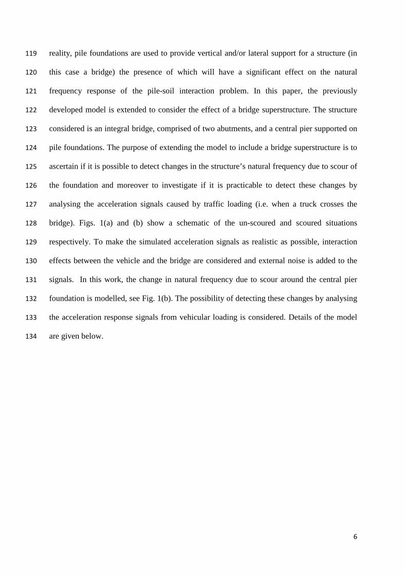
reality, pile foundations are used to provide vertical and/or lateral support for a structure (in 119
this case a bridge) the presence of which will have a significant effect on the natural 120
frequency response of the pile-soil interaction problem. In this paper, the previously 121
developed model is extended to consider the effect of a bridge superstructure. The structure 122
considered is an integral bridge, comprised of two abutments, and a central pier supported on 123
pile foundations. The purpose of extending the model to include a bridge superstructure is to 124
ascertain if it is possible to detect changes in the structure’s natural frequency due to scour of 125
the foundation and moreover to investigate if it is practicable to detect these changes by 126
analysing the acceleration signals caused by traffic loading (i.e. when a truck crosses the 127
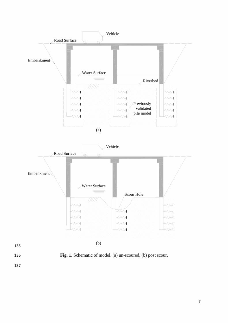
bridge). Figs. 1(a) and (b) show a schematic of the un-scoured and scoured situations 128
respectively. To make the simulated acceleration signals as realistic as possible, interaction 129
effects between the vehicle and the bridge are considered and external noise is added to the 130
signals. In this work, the change in natural frequency due to scour around the central pier 131
foundation is modelled, see Fig. 1(b). The possibility of detecting these changes by analysing 132
the acceleration response signals from vehicular loading is considered. Details of the model 133
are given below. 134
7
135
Fig. 1. Schematic of model. (a) un-scoured, (b) post scour. 136
137
Road Surface
Water Surface
Riverbed
Embankment
Vehicle
Previouslyvalidated
pile model
(a)
Road Surface
Water Surface
Scour Hole
Embankment
Vehicle
(b)

8
Bridge structure to be modelled 138
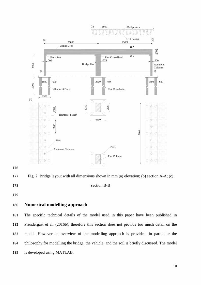
The bridge modelled is a two-span concrete integral bridge. A Young’s modulus of E = 139
3.5x10¹⁰ N m-2 and a material density of r = 2400 kg m-3 are assumed for all bridge elements. 140
For this type of bridge the abutment is formed using a series of vertical concrete columns and 141
reinforced earth. The columns support the deck and the reinforced earth retains the 142
embankment fill, see Fig. 2. The bridge is not intended to represent any particular real-life 143
structure. However, the properties were chosen to be representative of bridges of this type. 144
The bridge deck is comprised of nine U10 concrete bridge beams (Concast 2014). Each beam 145
supports a 200 mm deep deck slab giving a total combined moment of inertia of I = 2.9487 146
m4 and a cross-sectional area of A = 9.516 m2 for the bridge deck, which are typical values 147
for this type of bridge. The abutment consists of nine concrete columns supporting the bridge 148
deck, each column is 500 mm in diameter and the columns are at 1900 mm centres, see Fig. 149
2(c). This results in a total moment of inertia of I = 0.0276 m4 and a cross-sectional area of A 150
= 1.7671 m2 for the abutment elements. This type of bridge does not have a conventional 151
expansion joint so the thermal movements of the deck have to be accommodated by lateral 152
movements of the abutment columns. To facilitate this movement, the abutment columns are 153
cast in vertical sleeves so that there is a gap of 50 to 100 mm on all sides, i.e. the reinforced 154
earth provides no lateral restraint to the columns. These abutment columns are therefore 155
assumed free to move laterally. Two large concrete piers support the bridge at the centre and 156
have plan dimensions of 1375 mm x 2625 mm. This results in a total combined moment of 157
inertia of I = 1.137 m4 and a cross-sectional area of A = 7.22 m2 for the combined bridge pier 158
element. The piers are large stiff elements and they provide lateral restraint to the bridge 159
deck. 160
The abutment columns each rest on a pilecap, under which ten 15 m long concrete bored piles 161
are used as the foundation system, see Fig. 2. The pier columns each rest on a pilecap 162

9
supported by four piles. The scour action is assumed to be uniform along the transverse 163
length of a given support, so for modelling purposes, the structure shown in Fig. 2 is idealised 164
as the 2D frame shown in Fig. 3. (Note: scour is assumed to be equal on both sides of the 165
pier). The properties of each of the elements of the model in Fig. 3 are calculated by 166
summing the properties of the individual components shown in Fig. 2. For example, the 167
moment of inertia of the left abutment column shown in Fig. 3 is calculated by summing the 168
moment of inertia of the nine abutment columns shown in Fig. 2. Similarly the stiffness of the 169
two leaves of the pier shown in Section A-A of Fig. 2 is attributed to the central pier element 170
of Fig. 3. When apportioning stiffness to the pile elements shown in Fig. 3, a similar 171
philosophy was adopted. The abutment piles modelled have a combined cross-sectional area 172
of A = 2.827 m2 and a moment of inertia of I = 0.0636 m4 whereas the central pier piles have 173
A = 3.534 m2 and I = 0.1243 m4. Details on the spring stiffness coefficients used to model the 174
soil are given below and are summarised in Fig. 4. 175
10
176
Fig. 2. Bridge layout with all dimensions shown in mm (a) elevation; (b) section A-A; (c) 177
section B-B 178
179
Numerical modelling approach 180
The specific technical details of the model used in this paper have been published in 181
Prendergast et al. (2016b), therefore this section does not provide too much detail on the 182
model. However an overview of the modelling approach is provided, in particular the 183
philosophy for modelling the bridge, the vehicle, and the soil is briefly discussed. The model 184
is developed using MATLAB. 185
6000
25000 25000
500 1375 500
750
1600
2500
A A
Bridge Deck
AbutmentColumns
Bridge Pier
Pier Foundation
Pier Cross-HeadBank Seat
Abutment Piles
6001800 6001800
1500
0
3800
1900 32
50
2625
1710
0
3500
4500
Piles
Pier Column
Piles
Abutment Columns
Reinforced Earth
(a)
(b)
(c) Bridge deck1900
BB
200U10 Beams
11
186
Bridge model 187
The elements used in the bridge model are 6 degree-of-freedom (DOF) Euler-Bernoulli frame 188
elements (Kwon and Bang 2000). Each frame element has two nodes and each node has an 189
axial, transverse and a rotational degree of freedom as shown in the insert in Fig. 3. 190
The global mass and stiffness matrices for the model are assembled together according to the 191
procedure outlined in Kwon and Bang (2000). Damping is modelled using a Rayleigh 192
damping approach, with a damping ratio of 2% being assumed for all simulations in this 193
paper. The dynamic response of the bridge is obtained by solving the second order matrix 194
differential equation shown in Eq. (1). 195
( ) ( ) ( ) ( )tttt FKxxCxM =++ (1) 196
where M, C and K are the (nDOF × nDOF) global consistent mass, damping and stiffness 197
matrices respectively, and nDOF is the total number of degrees of freedom in the system. The 198
vector ( )tx describes the displacement of every degree of freedom for a given time step in 199
the analysis. Similarly, the vectors ( )tx and ( )tx describe the velocity and acceleration of 200
every degree of freedom in the model for the same time step. The vector ( )tF describes the 201
external forces acting on each degree of freedom for a given time step in the analysis. Eq. (1) 202
is solved using a numerical integration scheme, the Wilson-theta method (Dukkipati 2009). 203
Mode shapes and natural frequencies were extracted from the model by performing an 204
eigenvalue analysis on the system. In order to verify that the model was operating correctly, 205
the static displacements, mode shapes and natural frequencies predicted by the model were 206
verified against those calculated by a commercially available finite-element package. Good 207
agreement was observed between the model and the commercial software. 208
209

12
Vehicle model 210
The vehicle model, used in this work is similar to the model described in Hester and 211
González (2012) and González and Hester (2013). The vehicle model has four degrees of 212
freedom, namely a vertical displacement for each of the two axles (y1 and y2), the body 213
bounce (yb) and body pitch (φp), see Fig. 3. The body has mass mb and has rotational moment 214
of inertia Ip (for pitch). The body is supported on a suspension/axle assembly. The mass of 215
the wheel/axle assembly is mw. The suspension has a stiffness Ks and a damping coefficient 216
Cs. Finally, the tyre is modelled as a spring with stiffness Kt. Table 1 provides the parameters 217
of the vehicle (Cantero et al. 2011; El Madany 1988). Using the properties given in Table 1, 218
stiffness Kv, mass Mv and damping Cv matrices for the vehicle can be populated. The natural 219
frequencies of the vehicle for bounce, pitch, and front and rear axle hops are 1.43 Hz, 2.07 220
Hz, 8.860 Hz and 10.22 Hz respectively. 221
Table 1. Parameters of vehicle model. 222
Parameter Property Value
Dimensions (m) Wheel base (S) 5.5 Dist from centre of mass to front axle (S1) 3.66 Dist from centre of mass to rear axle (S2) 1.84
Mass (kg) Front wheel/axle mass (mw1) 700 Rear wheel/axle mass (mw2) 1,100 Sprung body mass (mb) 13,300
Inertia (kg m2) Pitch moment of inertia of truck (Ip) 41,008
Spring stiffness (kN m-1) Front axle (Ks1) 400 Rear axle (Ks2) 1,000
Damping (kN s m-1) Front axle (Cs1) 10 Rear axle (Cs2) 10
Tyre stiffness (kN m-1) Front axle (Kt1) 1,750 Rear axle (Kt2) 3,500
223
224
13
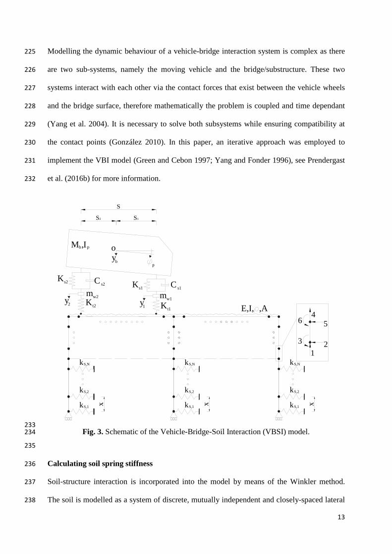
Modelling the dynamic behaviour of a vehicle-bridge interaction system is complex as there 225
are two sub-systems, namely the moving vehicle and the bridge/substructure. These two 226
systems interact with each other via the contact forces that exist between the vehicle wheels 227
and the bridge surface, therefore mathematically the problem is coupled and time dependant 228
(Yang et al. 2004). It is necessary to solve both subsystems while ensuring compatibility at 229
the contact points (González 2010). In this paper, an iterative approach was employed to 230
implement the VBI model (Green and Cebon 1997; Yang and Fonder 1996), see Prendergast 231
et al. (2016b) for more information. 232
233 Fig. 3. Schematic of the Vehicle-Bridge-Soil Interaction (VBSI) model. 234
235
Calculating soil spring stiffness 236
Soil-structure interaction is incorporated into the model by means of the Winkler method. 237
The soil is modelled as a system of discrete, mutually independent and closely-spaced lateral 238
kS,1
kS,2
kS,N
x
y2 y1Kt2 Kt1
mw2 mw1
Ks2 Ks1C s2 C s1
Mb Ip, oyb
p
S2 S1
S
kS,1
kS,2
kS,N
x kS,1
kS,2
kS,N
xE,I, ,A
1
4
2
5
3
6

14
springs (Dutta and Roy 2002; Winkler 1867). The method for developing spring stiffness 239
values is based on Prendergast et al. (2013) who derived spring stiffness values using the 240
small-strain shear modulus (G0) profile from their experimental site. Full details on 241
calculating soil spring stiffness coefficients is available in Prendergast and Gavin (2016a) and 242
Prendergast et al. (2015). The spring stiffness profiles used in this paper are shown in Fig. 4 243
for loose, medium-dense and dense sand. The individual spring stiffness moduli are shown by 244
the data markers on the plot. These profiles are for the central pier foundation piles. 245
246
Fig. 4. Postulated soil spring stiffness profiles for a loose, medium-dense and dense sand 247
around the central pier piles (N m-1) for the analysis. 248
249
Analysis & results 250
In the analyses performed using the model described previously, a moving vehicle excites the 251
bridge. The lateral response of the bridge is excited by the vehicle moving over the bridge, 252
inducing moments at the head of the abutments and the pier causing lateral sway. Horizontal 253
vehicle forces that would be induced by vehicle acceleration and braking are not included in 254
the model. However, these may contribute to the lateral response on a real system. The 255
vehicle crosses the bridge at typical highway speed and the horizontal acceleration from the 256
15
top of the pier is recorded and analysed. The effect of (initial) soil stiffness on the frequency 257
changes with scour was examined for the three soil stiffness profiles. To aid in choosing 258
appropriate locations to place accelerometers on the structure and to ascertain a baseline for 259
the expected change in natural frequency due to scour, an eigenvalue modal analysis was 260
conducted in the first instance. 261
262
Eigen frequencies and mode shapes 263
An eigenvalue analysis was conducted in the model to extract the fundamental frequency of 264
(lateral) vibration for different depths of scour. A maximum scour depth of 10 m was 265
considered in the model and the difference in frequency between zero scour and this 266
maximum value is shown in Table 2. The results indicate that a scour depth of 10 m produced 267
a change in fundamental frequency of ≈ 40 % for the three soil stiffness profiles considered. 268
Once the expected shift in frequency due to scour was established, the next step was to 269
determine the optimum points on the structure to record accelerations to give the best 270
opportunity to capture the first mode of vibration of the integral bridge. By plotting the first 271
mode shape of the structure for zero scour and full pier scour, it is possible to obtain a 272
pictorial view of the locations showing the highest modal displacements for the fundamental 273
mode. Fig. 5 shows that the first mode shape for both zero scour and maximum pier scour 274
(10 m) is a global sway mode. The data shown in Fig. 5 was for the analysis performed in 275
loose sand. However, the shape was the same for all three soil stiffness profiles considered. 276
From the figure, it can be seen that the maximum modal amplitude occurs at deck level. In 277
this study the top of the bridge pier is used as the location to measure acceleration as it assists 278
in identifying the frequency when using signal processing and also aids with signal to noise 279
ratio (SNR) issues. 280

16
Table 2. Eigenvalue analysis of the scour effect. 281
Scour depth (m) Frequency (loose sand) (Hz)
Frequency (medium dense sand) (Hz)
Frequency (dense sand) (Hz)
0 m 1.5643 1.6481 1.7357 10 m (full) 0.9386 0.9772 1.017 % Difference -39.99% -40.708% -41.4% 282
283
Fig. 5. Fundamental mode shapes in loose sand – global sway. (a) zero scour (b) full scour. 284
285
Response of structure to moving half-car vehicle model 286
Simulation of noise free pier accelerations due to the passage of a vehicle 287
From the eigenvalue analysis in the previous section, it was observed that significant 288
reductions in natural frequency occurred due to scour of the central pile foundation system. 289
However, the fact that frequency changes will occur is of little use if the relevant mode is not 290
excited in the structure. The most practical way to excite a rail / highway bridge is to use 291
ambient traffic (Farrar et al. 1999). Therefore in this section the aim is to ascertain if it is 292
possible to detect these frequency changes by analysing the bridge acceleration response to a 293

17
moving sprung vehicle. In this analysis, accelerations generated at a lateral degree of freedom 294
near the top of the bridge pier are analysed using a fast Fourier transform to obtain the 295
frequency content. The vehicle modelled is a 15 tonne two-axle truck (see Table 1), and to 296
make the model as realistic as possible interaction between the vehicle and the bridge is 297
allowed for. The bridge is excited by the sudden arrival of the vehicle on the bridge deck, 298
which effectively acts as an impulse load. 299
The vehicle is a four-degree-of-freedom system that moves along the bridge deck. The 300
vehicle is excited by the presence of a road profile which causes the body to pitch and bounce 301
and this in turn means that the forces that the vehicle applies to the bridge are not constant. In 302
the model the vehicle commences movement at an approach distance of 100 m from the start 303
of the bridge so that the initial vehicle motion conditions (axle displacements and body 304
displacement / pitch) when the vehicle meets the bridge are more realistic. The road profile 305
used in the current analysis is a Class ‘A’ profile (well-maintained road surface, see Cebon 306
(1999)), and the part of the road profile on the bridge is reproduced in Fig. 6. This figure also 307
shows a Class ‘B’ and a Class ‘C’ road profile, in order of degrading quality. 308
309
Fig. 6. Road profiles on the bridge. 310
311
18
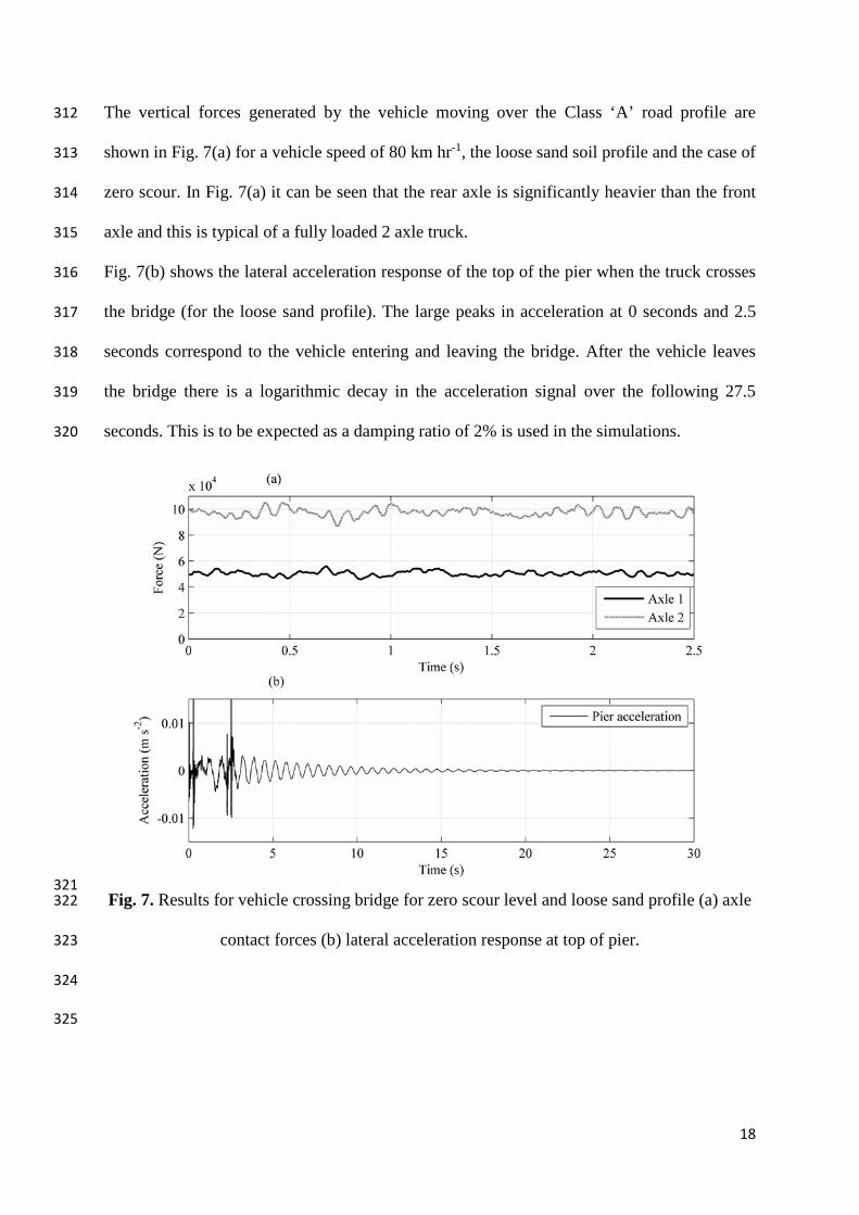
The vertical forces generated by the vehicle moving over the Class ‘A’ road profile are 312
shown in Fig. 7(a) for a vehicle speed of 80 km hr-1, the loose sand soil profile and the case of 313
zero scour. In Fig. 7(a) it can be seen that the rear axle is significantly heavier than the front 314
axle and this is typical of a fully loaded 2 axle truck. 315
Fig. 7(b) shows the lateral acceleration response of the top of the pier when the truck crosses 316
the bridge (for the loose sand profile). The large peaks in acceleration at 0 seconds and 2.5 317
seconds correspond to the vehicle entering and leaving the bridge. After the vehicle leaves 318
the bridge there is a logarithmic decay in the acceleration signal over the following 27.5 319
seconds. This is to be expected as a damping ratio of 2% is used in the simulations. 320
321 Fig. 7. Results for vehicle crossing bridge for zero scour level and loose sand profile (a) axle 322
contact forces (b) lateral acceleration response at top of pier. 323
324
325

19
The effect of noise on determining the frequency of the pier vibrations 326
Real data will contain noise, so in this study, noise was added to the simulated signal. In 327
order to check if the (scour detection) method was sensitive to the level of noise in the signal, 328
signals with different levels of noise are analysed. The method used to add noise is based on 329
the signal-to-noise ratio (SNR), given in Eq. (2) (Lyons 2011). 330
Power NoisePower Signallog10 10=SNR (2) 331
where SNR is the ratio of the strength of a signal carrying information equating to that of 332
unwanted interference. Eq. (2) is rearranged to give Eq. (3). 333
( )
==
1010SNR.log
exp
Power SignalPower Noise e
Nσ (3) 334
where Nσ is the noise variance. Using Eq. (3), noise signals with different signal-to-noise 335
ratios were added to the original clean signal. This process is shown in Eq. (4). 336
[ ] CLEANNOISE SigSig += randNσ (4) 337
In this study, three noise levels were examined, namely SNRs of 20, 10 and 5. Figs. 8(a-c) 338
show the result of adding noise to the signal shown in Fig. 7(b). Fig. 8(d) shows the 339
frequency content of the signals in Fig. 8(a-c). It can be seen in the figure that for all levels of 340
noise the frequency plot is practically identical which proves that the method will not be 341
particularly sensitive to noise. For the purpose of completeness, the figure has an insert which 342
shows a zoomed in view of the frequency peak. In the insert it can be seen that that there are 343
small differences in the frequency peak for the different levels of noise. However, in relative 344
terms these differences are insignificant. Since noise does not impede the ability of the 345
method to detect the frequency accurately, all analysis from this point will contain a SNR = 346
20 as it is easier for the reader to interpret the remaining time domain plots for lower values 347
of noise. 348

20
349
Fig. 8. Sensitivity of frequency content to noise. (a) signal from bridge pier with SNR = 20, 350
(b) signal with SNR = 10, (c) signal with SNR = 5, (d) frequency content of signals shown in 351
Figs. 8(a)-(c). 352
353
Effect of vehicle properties, driving speed and road profile on detecting the frequency of the pier 354
vibrations 355
In the previous section, it was established that artificially added noise does not significantly 356
impede the method of detecting the first natural frequency of the structure (global sway) from 357
the pier accelerations due to a passing vehicle. However, the analysis in the previous section 358
only considers one set of vehicle properties, one driving speed and a Class ‘A’ road profile. 359
In this section, the effect of varying the driving speed, vehicle properties and road roughness 360
condition on the resilience of the method is investigated. Fig. 9 shows the effect of varying 361
the vehicle driving speed on the detected first natural frequency of the bridge. In this figure, 362
the vehicle traverses the bridge at 50, 80 and 100 km hr-1 and the lateral acceleration signal 363
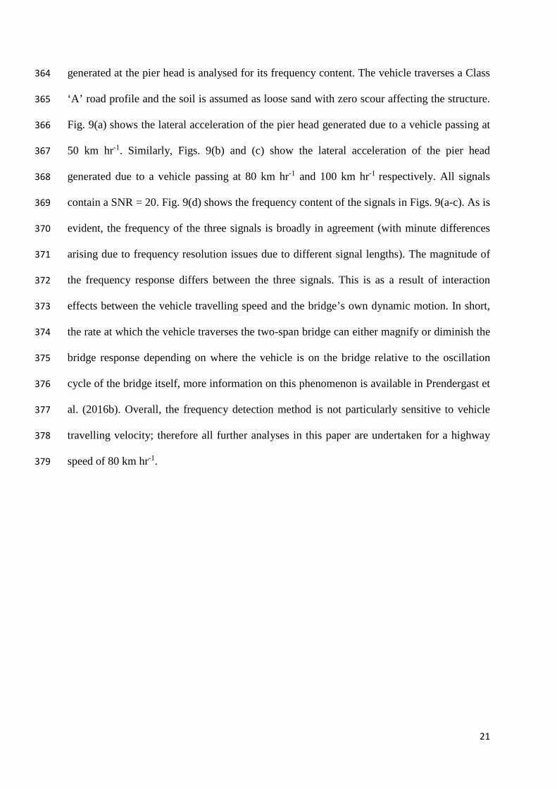
21
generated at the pier head is analysed for its frequency content. The vehicle traverses a Class 364
‘A’ road profile and the soil is assumed as loose sand with zero scour affecting the structure. 365
Fig. 9(a) shows the lateral acceleration of the pier head generated due to a vehicle passing at 366
50 km hr-1. Similarly, Figs. 9(b) and (c) show the lateral acceleration of the pier head 367
generated due to a vehicle passing at 80 km hr-1 and 100 km hr-1 respectively. All signals 368
contain a SNR = 20. Fig. 9(d) shows the frequency content of the signals in Figs. 9(a-c). As is 369
evident, the frequency of the three signals is broadly in agreement (with minute differences 370
arising due to frequency resolution issues due to different signal lengths). The magnitude of 371
the frequency response differs between the three signals. This is as a result of interaction 372
effects between the vehicle travelling speed and the bridge’s own dynamic motion. In short, 373
the rate at which the vehicle traverses the two-span bridge can either magnify or diminish the 374
bridge response depending on where the vehicle is on the bridge relative to the oscillation 375
cycle of the bridge itself, more information on this phenomenon is available in Prendergast et 376
al. (2016b). Overall, the frequency detection method is not particularly sensitive to vehicle 377
travelling velocity; therefore all further analyses in this paper are undertaken for a highway 378
speed of 80 km hr-1. 379

22
380
Fig. 9. Sensitivity of frequency content to vehicle speed. (a) signal from bridge pier with 381
vehicle speed = 50 km hr-1, (b) signal with vehicle speed = 80 km hr-1, (c) signal with vehicle 382
speed = 100 km hr-1, (d) frequency content of signals shown in Figs. 9(a)-(c). 383
384
The vehicle modelled in the simulations undertaken previously is a two axle truck, the 385
properties of which are shown in Table 1. In order to assess if the vehicle properties have any 386
noticeable effect on the ability of the method to detect the bridge’s first frequency from 387
vehicle induced lateral motion, a brief analysis is conducted herein. For this analysis, the 388
vehicle whose properties are outlined in Table 1 (Veh 1) is run across the bridge and 389
compared to a modified vehicle (Veh 2), which includes an altered front axle stiffness and 390
gross body mass. The relevant properties of both vehicles are outlined in Table 3. 391
392
393
394

23
Table 3. Veh 1 and Veh 2 properties for sensitivity analysis. 395
Veh 1 Veh 2 Gross body mass (kg) 13,300 9,000 Front axle stiffness (kN m-1) 400 600 Body bounce frequency (Hz) 1.43 1.84 396
The result of running both vehicles over the bridge is shown in Fig. 10. Both vehicles traverse 397
at 80 km hr-1 over a bridge with zero scour, a loose sand profile and a Class ‘A’ road surface. 398
Signals contain a SNR = 20. Fig. 10(a) shows the lateral pier head acceleration due to the 399
passage of the original vehicle (Veh 1). Fig. 10(b) shows the lateral pier head acceleration 400
due to the passage of the modified vehicle (Veh 2). Fig. 10(c) shows the frequency content of 401
the signals in (a) and (b). As is evident, altering the vehicle properties does not significantly 402
affect the frequency detection method, as the frequency is identical with only a minor change 403
in magnitude. The analysis conducted here only considers a two-axle truck, however, so the 404
effect for other vehicle types is not considered. 405
406
Fig. 10. Sensitivity of frequency content to vehicle mass and axle stiffness. (a) signal from 407
bridge pier with original vehicle properties, (b) signal with modified vehicle properties (c) 408
frequency content of signals shown in Figs. 10(a) and (b). 409

24
410
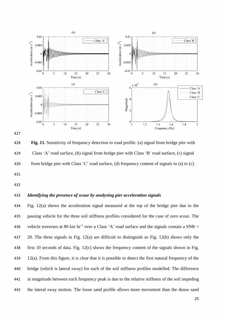
Finally, it is of interest to assess if a degrading road surface will impede the ability for the 411
first natural sway frequency of the bridge to be detected from vehicle induced vibrations. For 412
this analysis, the original vehicle (Veh 1) traverses the bridge over a Class ‘A’, ‘B’ and ‘C’ 413
profile at 80 km hr-1 for the case of zero scour (see Fig. 6 for road profiles). All signals 414
contain a SNR = 20. The results are shown in Fig. 11. Fig. 11(a) shows the lateral pier head 415
acceleration due to the vehicle traversing a Class ‘A’ road profile. Similarly, Figs. 11(b) and 416
(c) show the lateral pier head accelerations measured due to a vehicle traversing Class ‘B’ 417
and ‘C’ profiles respectively. Fig. 11(d) shows the frequency content of the signals presented 418
in parts (a) to (c) of the figure. The frequency peak corresponding to the first natural 419
frequency of the bridge is clearly detected in all three signals, with differences in magnitude 420
occurring for each road roughness profile. From this figure, it is clear that the presence of a 421
road roughness profile up to Class ‘C’ does not significantly impede the ability for the bridge 422
frequency peak to be detected (only very minor differences in frequency are detected due to 423
resolution of frequency bins). As a result, all analyses from here will utilise a Class ‘A’ 424
profile, equivalent to a well-maintained highway surface. In the next section, the detection of 425
scour from pier head lateral accelerations is investigated. 426
25
427
Fig. 11. Sensitivity of frequency detection to road profile. (a) signal from bridge pier with 428
Class ‘A’ road surface, (b) signal from bridge pier with Class ‘B’ road surface, (c) signal 429
from bridge pier with Class ‘C’ road surface, (d) frequency content of signals in (a) to (c). 430
431
432
Identifying the presence of scour by analysing pier acceleration signals 433
Fig. 12(a) shows the acceleration signal measured at the top of the bridge pier due to the 434
passing vehicle for the three soil stiffness profiles considered for the case of zero scour. The 435
vehicle traverses at 80 km hr-1 over a Class ‘A’ road surface and the signals contain a SNR = 436
20. The three signals in Fig. 12(a) are difficult to distinguish so Fig. 12(b) shows only the 437
first 10 seconds of data. Fig. 12(c) shows the frequency content of the signals shown in Fig. 438
12(a). From this figure, it is clear that it is possible to detect the first natural frequency of the 439
bridge (which is lateral sway) for each of the soil stiffness profiles modelled. The difference 440
in magnitude between each frequency peak is due to the relative stiffness of the soil impeding 441
the lateral sway motion. The loose sand profile allows more movement than the dense sand 442

26
profile (due to the difference in spring stiffness); hence a higher peak was observed for the 443
loose sand. 444
445
Fig. 12. Bridge response due to passing vehicle and subsequent free vibration. (a) 446
acceleration response from bridge pier for loose, medium-dense and dense sand profiles with 447
40 seconds of free vibration; (b) acceleration response from bridge pier for loose, medium-448
dense and dense sand profiles with 7.5 seconds of free vibration; (c) frequency response of 449
signals shown in (a). 450
451
Fig. 12 demonstrates that the natural frequency of mode 1 can be accurately determined by 452
analysing the acceleration response of the pier with a Fourier transform for all three soil 453

27
densities. The next step is to induce scour in the analysis and observe the change in 454
frequency. An example of this analysis is shown in Fig. 13. The analysis involved running the 455
vehicle over the bridge to generate an acceleration signal at the top of the bridge pier and 456
adding noise. This signal was then analysed with a fast Fourier transform to determine the 457
frequency content of the signal. A scour depth of 10 m is induced by removing springs from 458
around the central pier foundation and the process is repeated to generate a scoured signal. 459
The solid and dashed plots in Fig. 13(a) shows the acceleration signals generated at the top of 460
the bridge pier for the case of zero scour and the 10 m scour depth respectively, (for a loose 461
sand profile). For ease of visualising the signals, Fig. 13(b) shows just the first 10 seconds of 462
the pier acceleration responses. On the left hand side of this plot, a total of four impulses in 463
the acceleration signals (between t = 0 and t = 2.5 s) are visible. This corresponds to the front 464
and rear axles entering and leaving the bridge. The front axle enters the bridge at t = 0 s and 465
the rear axle leaves the bridge at t = 2.5 s. Fig. 13(c) shows the frequency content of the 466
signals shown in Fig. 13(a). It can be seen in Fig. 13(c) that the natural frequency for zero 467
scour was 1.556 Hz. It can also be seen in Fig. 13(c) that the natural frequency at the 468
maximum scour depth of 10 m was 0.9308 Hz. Therefore, a significant and measureable 469
reduction in natural frequency was observed. 470

28
471
Fig. 13. Effect of 10 m of scour on the pier acceleration response for loose sand profile. (a) 472
acceleration response (laterally) at top of bridge pier for zero and 10 m scour due to passage 473
of vehicle, including 40 seconds of free vibration; (b)acceleration response of bridge pier 474
with 7.5 seconds of free vibration; (c) frequency content of signals shown in (a). 475
476
By repeating the analysis for scour depths ranging from 0.5 m to 10 m, the natural frequency 477
for each scour depth was determined. Scour was induced around the central pier piled 478
foundation by removing springs iteratively from the model, this corresponds to an increase in 479
scour depth and a loss of associated soil stiffness. A spring is removed and the vehicle is re-480
run across the bridge to generate a new acceleration signal, which is analysed for its 481
frequency content. The variation in natural frequency with scour depth for the ‘loose sand’ is 482

29
shown by the solid plot with circular data markers in Fig. 14. Fig. 14 also shows the change 483
in the natural frequency plotted against the depth of scour for the ‘medium-dense sand’ and 484
‘dense sand’ stiffness profiles. It is clear from this figure that for the three soil stiffness 485
profiles simulated, it was possible to detect a change in the natural frequency of the bridge 486
due to scour using vehicle induced vibrations. It is worth noting that the method was not 487
sensitive to soil stiffness (loose, medium-dense or dense) i.e. for all soil densities considered, 488
there is a clear reduction in natural frequency with increasing scour. Not surprisingly, the 489
magnitude of the frequency for a given scour depth varies with the soil stiffness. However, 490
the variation with soil stiffness is significantly less than the variation with scour depth. This 491
basically implies that the increase in effective length resulting from scour had a much larger 492
effect on the frequency response of the structure than changes in the stiffness of the soil 493
supporting the foundation. 494
495
Fig. 14. Frequency change with scour for all three soil stiffness profiles. 496
497
498
30
Conclusion 499
A field-validated model developed by the authors which is capable of tracking the change in 500
the natural frequency of a single pile affected by scour was extended in this paper to consider 501
the case of a full bridge subjected to traffic loading. A novel Vehicle-Bridge-Soil Interaction 502
(VBSI) model was developed to explore the potential frequency changes due to scour of an 503
integral bridge structure for a range of soil stiffnesses typically found in the field. 504
In the first instance, it was necessary to establish how scour affects the natural frequency of 505
the bridge and if the changes in frequency would be sufficiently large to warrant further 506
exploration of this method as a potential scour monitoring tool. A numerical modal study was 507
conducted to address this question. The aim of this study was to assess the magnitude of 508
frequency changes that can be expected for a typical bridge structure subjected to scour of the 509
central piles. From this study, the expected magnitude of the frequency shift was established 510
and deemed sufficiently large (≈ 40%) to warrant an investigation into the feasibility of 511
detecting scour by analysing the bridge’s response to a moving vehicle. The VBSI model was 512
used to generate realistic acceleration signals from the structure due to a two-axle truck 513
passing at typical highway speeds (80 km hr-1). The lateral acceleration response at the top of 514
the bridge pier was analysed. Results indicate that for all three soil stiffness profiles modelled 515
(loose, medium-dense and dense sand) the response signals generated from this vehicular 516
loading are sufficient to allow the changes in natural frequency caused by scour to be 517
detected. Moreover, the shape of the scour depth vs frequency plot was the same for all three 518
soil stiffness profiles which shows that the method is not sensitive to soil stiffness. 519
Limitations in the analysis include the fact that only one type of vehicle was modelled, 520
namely a two-axle truck. Therefore the conclusions of the present study may only be relevant 521
for this vehicle type. Also, since the method relies on frequency changes of the bridge being 522
detected to infer the presence of scour, this method would be sensitive to other forms of 523
31
damage to the superstructure such as crack formation, thermal effects etc. Establishing the 524
exact mechanism causing the changes in frequency requires further study, and is not 525
addressed in this paper. The current paper serves as a feasibility study to detect the presence 526
of scour from vehicle-induced vibrations. 527
The method developed in this paper shows promise in terms of use as part of an infrastructure 528
management framework incorporating real-time low maintenance scour monitoring. The 529
advantage of the method is that it does not require complex underwater installations and 530
negates the requirement for dangerous diving inspections to monitor scour. The results 531
indicate that accelerometers fixed to the structure above the waterline may possibly be used 532
as a continuous scour monitoring solution. Real-time analysis of signals from a structure of 533
interest could be monitored for frequency changes or signals could be analysed before and 534
after major flood events to attempt to detect losses of stiffness caused by scour. Whilst this 535
appears promising, a full-scale application of the method on a real bridge is recommended as 536
future work. 537
538
Acknowledgements 539
The authors would like to acknowledge the support of the Earth and Natural Sciences (ENS) 540
Doctoral Studies Programme, funded by the Higher Education Authority (HEA) through the 541
Programme for Research at Third Level Institutions, Cycle 5 (PRTLI-5), co-funded by the 542
European Regional Development Fund (ERDF), the European Union Framework 7 project 543
SMART RAIL (Project No. 285683) and the European Union H2020 project DESTination 544
RAIL (Project No. 636285). 545
546
References 547
Abdel Wahab, M. M., and De Roeck, G. (1999). “Damage Detection in Bridges Using Modal 548

32
Curvatures: Application To a Real Damage Scenario.” Journal of Sound and Vibration, 549
226(2), 217–235. 550
Anderson, N. L., Ismael, A. M., and Thitimakorn, T. (2007). “Ground-Penetrating Radar : A 551
Tool for Monitoring Bridge Scour.” Environmental & Engineering Geoscience, XIII(1), 552
1–10. 553
Avent, R. R., and Alawady, M. (2005). “Bridge Scour and Substructure Deterioration : Case 554
Study.” Journal Of Bridge Engineering, 10(3), 247–254. 555
Briaud, J. L., Chen, H. C., Ting, F. C. K., Cao, Y., Han, S. W., and Kwak, K. W. (2001). 556
“Erosion Function Apparatus for Scour Rate Predictions.” Journal of Geotechnical and 557
Geoenvironmental Engineering, 105–113. 558
Briaud, J. L., Chen, H., Li, Y., Nurtjahyo, P., and Wang, J. (2005). “SRICOS-EFA Method 559
for Contraction Scour in Fine-Grained Soils.” Journal of Geotechnical and 560
Geoenvironmental Engineering, 131(10), 1283–1295. 561
Briaud, J. L., Hurlebaus, S., Chang, K., Yao, C., Sharma, H., Yu, O., Darby, C., Hunt, B. E., 562
and Price, G. R. (2011). Realtime monitoring of bridge scour using remote monitoring 563
technology. Security, Austin, TX. 564
Briaud, J. L., Ting, F., and Chen, H. C. (1999). “SRICOS: Prediction of Scour Rate in 565
Cohesive Soils at Bridge Piers.” Journal of Geotechnical and Geoenvironmental 566
Engineering, (April), 237–246. 567
Cantero, D., Gonzalez, A., and O’Brien, E. J. (2011). “Comparison of bridge dynamic 568
amplification due to articulated 5-axle trucks and large cranes.” Baltic Journal of Road 569
and Bridge Engineering, 6(1), 39–47. 570
Cebon, D. (1999). Handbook of Vehicle-Road Interaction. Swets & Zeitlinger, Netherlands. 571
Chen, C.-C., Wu, W.-H., Shih, F., and Wang, S.-W. (2014). “Scour evaluation for foundation 572
of a cable-stayed bridge based on ambient vibration measurements of superstructure.” 573
33
NDT & E International, Elsevier, 66, 16–27. 574
Concast. (2014). “Concast Precast Group.” Civil Engineering Solutions, 575
<http://www.concastprecast.co.uk/images/uploads/brochures/Concast_Civil.pdf> (May 576
1, 2014). 577
Doebling, S., and Farrar, C. (1996). Damage identification and health monitoring of 578
structural and mechanical systems from changes in their vibration characteristics: a 579
literature review. 580
Dukkipati, R. V. (2009). Matlab for Mechanical Engineers. New Age Science. 581
Dutta, S. C., and Roy, R. (2002). “A critical review on idealization and modeling for 582
interaction among soil–foundation–structure system.” Computers & Structures, 80(20-583
21), 1579–1594. 584
Elsaid, A., and Seracino, R. (2014). “Rapid assessment of foundation scour using the 585
dynamic features of bridge superstructure.” Construction and Building Materials, 586
Elsevier Ltd, 50, 42–49. 587
De Falco, F., and Mele, R. (2002). “The monitoring of bridges for scour by sonar and 588
sedimetri.” NDT&E International, 35, 117–123. 589
Farrar, C. R., Duffey, T. A., Cornwell, P. J., and Doebling, S. W. (1999). “Excitation 590
methods for bridge structures.” Proceedings of the 17th International Modal Analysis 591
Conference Kissimmee, Kissimmee, FL. 592
Fisher, M., Chowdhury, M. N., Khan, A. a., and Atamturktur, S. (2013). “An evaluation of 593
scour measurement devices.” Flow Measurement and Instrumentation, Elsevier, 33, 55–594
67. 595
Forde, M. C., McCann, D. M., Clark, M. R., Broughton, K. J., Fenning, P. J., and Brown, A. 596
(1999). “Radar measurement of bridge scour.” NDT&E International, 32, 481–492. 597
Foti, S., and Sabia, D. (2011). “Influence of Foundation Scour on the Dynamic Response of 598

34
an Existing Bridge.” Journal Of Bridge Engineering, 16(2), 295–304. 599
González, A. (2010). “Vehicle-Bridge Dynamic Interaction Using Finite Element 600
Modelling.” Finite-Element Analysis, 637–662. 601
González, A., and Hester, D. (2013). “An investigation into the acceleration response of a 602
damaged beam-type structure to a moving force.” Journal of Sound and Vibration, 603
332(13), 3201–3217. 604
Green, F., and Cebon, D. (1997). “Dynamic interaction between heavy vehicles and highway 605
bridges.” Computers and Structures, 62(2), 253–264. 606
Hamill, L. (1999). Bridge Hydraulics. E.& F.N. Spon, London. 607
Hester, D., and González, A. (2012). “A wavelet-based damage detection algorithm based on 608
bridge acceleration response to a vehicle.” Mechanical Systems and Signal Processing, 609
28, 145–166. 610
Ju, S. H. (2013). “Determination of scoured bridge natural frequencies with soil–structure 611
interaction.” Soil Dynamics and Earthquake Engineering, 55, 247–254. 612
Klinga, J. V., and Alipour, A. (2015). “Assessment of structural integrity of bridges under 613
extreme scour conditions.” Engineering Structures, Elsevier Ltd, 82, 55–71. 614
Kwon, Y. W., and Bang, H. (2000). The Finite Element Method using MATLAB. CRC Press, 615
Inc., Boca Raton, FL. 616
Lagasse, P. F., Schall, J. D., Johnson, F., Richardson, E. V., and Chang, F. (1995). Stream 617
stability at highway structures. Washington, DC. 618
Lyons, R. (2011). Understanding digital signal processing. Prentice Hall, Boston, MA. 619
El Madany, M. (1988). “Design and optimization of truck suspensions using covariance 620
analysis.” Computers & structures. 621
Melville, B. W., and Coleman, S. E. (2000). Bridge scour. Water Resources Publications, 622
Highlands Ranch, CO. 623
35
Prendergast, L. J., and Gavin, K. (2014). “A review of bridge scour monitoring techniques.” 624
Journal of Rock Mechanics and Geotechnical Engineering, 6(2), 138–149. 625
Prendergast, L. J., and Gavin, K. (2016a). “A comparison of initial stiffness formulations for 626
small-strain soil – pile dynamic Winkler modelling.” Soil Dynamics and Earthquake 627
Engineering, 81, 27–41. 628
Prendergast, L. J., Gavin, K., and Doherty, P. (2015). “An investigation into the effect of 629
scour on the natural frequency of an offshore wind turbine.” Ocean Engineering, 101, 1–630
11. 631
Prendergast, L. J., Hester, D., and Gavin, K. (2016b). “Development of a Vehicle-Bridge-Soil 632
Dynamic Interaction Model for Scour Damage Modelling.” Shock and Vibration, 2016. 633
Prendergast, L. J., Hester, D., Gavin, K., and O’Sullivan, J. J. (2013). “An investigation of 634
the changes in the natural frequency of a pile affected by scour.” Journal of Sound and 635
Vibration, 332(25), 6685–6702. 636
Sampaio, R. P. C., Maia, N. M. M., and Silva, J. M. M. (1999). “Damage Detection Using the 637
Frequency-Response-Function Curvature Method.” Journal of Sound and Vibration, 638
226(5), 1029–1042. 639
Shirole, A. M., and Holt, R. C. (1991). “Planning for a comprehensive bridge safety 640
assurance program.” Transport Research Record, Transport Research Board, 641
Washington, DC, 137–142. 642
Wardhana, K., and Hadipriono, F. C. (2003). “Analysis of Recent Bridge Failures in the 643
United States.” Journal of Performance of Constructed Facilities, 17(3), 144–151. 644
Winkler, E. (1867). Theory of elasticity and strength. Dominicus Prague. 645
Yang, F., and Fonder, G. (1996). “An iterative solution method for dynamic response of 646
bridge–vehicles systems.” Earthquake engineering & structural dynamics, 25, 195–215. 647
Yang, Y., Yau, J., and Wu, Y. (2004). Vehicle-bridge interaction dynamics. 648

36
Yankielun, N., and Zabilansky, L. (1999). “Laboratory Investigation of Time-Domain 649
Reflectometry System for Monitoring Bridge Scour.” Journal of Hydraulic Engineering, 650
125(12), 1279–1284. 651
Yu, X. (2009). “Time Domain Reflectometry Automatic Bridge Scour Measurement System: 652
Principles and Potentials.” Structural Health Monitoring, 8(6), 463–476. 653
Zarafshan, A., Iranmanesh, A., and Ansari, F. (2012). “Vibration-Based Method and Sensor 654
for Monitoring of Bridge Scour.” Journal Of Bridge Engineering, 17(6), 829–838. 655
656