PURE PHYSICS

FINAL YEAR PROJECT REPORT

ZCT 390/6

MOLECULAR DYNAMICS SIMULATION:

PHASE COEXISTENCE CURVE AND PROPERTIES OF

LENNARD-JONES FLUID

BY

SOON YEE YEEN

PROJECT SUPERVISOR

DR. YOON TIEM LEONG

THESIS SUBMITTED IN FULFILLMENT OF THE REQUIREMENTS

FOR THE DEGREE OF

BACHELOR OF SCIENCE (HONOURS) (PHYSICS)

JUNE 2013

i

ACKNOWLEDGEMENT

This project would not have been possible without the guidance and the help of several

individuals who in one way or another contributed and extended their valuable assistance in

the preparation and completion of this study.

First of all, I would like to express my deepest appreciation to my supervisor, Dr. Yoon

Tiem Leong, for his enthusiastic guidance in this project. He had also provided the useful

resources and exposed me to the ideas for doing this project. His enthusiasm, intelligence,

patience and encouragements have helped me mature in my studies and research.

Then, I would like to express my utmost gratitude to Universiti Sains Malaysia (USM)

and School of Physics, USM. This project was conducted in School of Physics, USM by

using the computer power provided in computer lab. With these advanced computer source, it

enable me to obtain results of project easier and faster compared to personal computer.

I would like to express my appreciation to all the staffs in School of Physics, USM, for

giving us a comfortable environment and well-operating system to work on our project.

Thanks to the staffs that are in charge of computer lab, we are able to use the computer

clusters to conduct our simulations.

In addition, I would like to express my gratitude to my project partner, Mr. Goh Eong

Sheng. The opinion and knowledge provided by him are very useful in project. He is patient

to explain to me when I faced problem. Also, his encouragement given for this period of time

makes our project to be conducted smoothly.

Last but not least, I would also like to thank my parents my friends, for their continuous

and constant support throughout this period of time. Special thanks to our seniors who are

also constantly supporting me and sharing experience and expertise with us. Their valuable

suggestions are very helpful in conducting my project and studies.

ii

TABLE OF CONTENTS

Acknowledgements i

Table of Contents ii

List of Abbreviations v

List of Symbols vi

List of Figures vii

List of Tables ix

Abstrak x

Abstract xii

1. Introduction 1

1.1 Objective and Problem Statement ................................................................................1

1.2 Computer Simulations of Molecular Systems ..............................................................2

1.3 Acknowledgement of Previous Work ..........................................................................4

1.4 Scope and Content ........................................................................................................4

2. Literature Review 6

2.1 Classical Simulation of Lennard-Jones System ...........................................................6

2.2 Derived Equations of State ...........................................................................................7

2.3 Applications of Molecular Simulations ........................................................................8

2.3.1 Monte Carlo Simulation .....................................................................................8

2.3.2 Molecular Dynamics Simulation .......................................................................8

2.4 Scope and Methods of Molecular Simulations .............................................................9

2.5 Temperature-Quench Molecular Dynamics Simulations ...........................................10

3. Theory 11

3.1 Molecular Simulation .................................................................................................11

3.2 Lennard-Jones Potential .............................................................................................12

3.3 Reduced Units ............................................................................................................13

iii

3.4 Periodic Boundary Condition .....................................................................................15

3.5 Molecular Dynamics Simulations ..............................................................................17

3.5.1 Classical Approach ..........................................................................................17

3.5.2 Newtonian Mechanics ......................................................................................17

3.5.3 Numerical Integration ......................................................................................18

3.5.3.1 Velocity Verlet Method ......................................................................19

3.5.3.2 Truncation of Interactions ..................................................................20

3.5.3.3 Instantaneous Temperature .................................................................21

3.5.3.4 Instantaneous Pressure .......................................................................22

3.5.3.5 Berendsen Thermostat ........................................................................22

3.5.3.6 Berendsen Barostat .............................................................................22

3.5.3.7 Radial Distribution Function ..............................................................23

3.5.3.8 Ideal and Real Gases ..........................................................................24

3.5.4 Summary ..........................................................................................................25

4. Methodology 26

4.1 Overview ....................................................................................................................26

4.1.1 Temperature-Quench Molecular Dynamics .....................................................26

4.1.2 Study of Properties of Lennard-Jones Potential...............................................27

4.2 Temperature-Quench Molecular Dynamics ...............................................................27

4.2.1 Overall Process Flow .......................................................................................27

4.2.2 Preparing and Quenching of System................................................................28

4.2.3 Interface Detection and Elimination ................................................................29

4.2.4 Determination of Equilibrium Properties .........................................................31

5. Results and Discussion 32

5.1 Temperature-Quench Molecular Dynamics ...............................................................32

5.1.1 Vapour-Liquid Coexistence Curve ..................................................................32

5.1.2 Comparison with TQMD by Müler .................................................................34

5.1.3 Comparison with GEMC by Müler..................................................................35

5.1.4 Comparison by Using Different Total Simulation Steps .................................36

5.1.5 Comparison with Standard Values for Various Noble Gases ..........................39

5.1.6 Comparison by Using Different Methods of Molecular Simulations ..............41

5.2 Properties of Lennard-Jones Fluid..............................................................................42

iv

5.2.1 Observations Indicating Phase Transition .......................................................42

5.2.2 Relation Between Temperature and Density ...................................................42

5.2.3 Relation Between Pressure and Temperature ..................................................45

5.2.4 Relation Between Pressure and Volume ..........................................................46

6. Conclusion and Recommendations 49

6.1.1 Conclusion .......................................................................................................49

6.1.2 Recommendations ............................................................................................50

7. References 51

8. Appendix 54

v

LIST OF ABBREVIATIONS

LJ Lennard-Jones

MD Molecular dynamics

MC Monte Carlo

TQMD Temperature-quench molecular dynamics

GEMC Gibbs ensemble Monte Carlo

VEMD Volume expansion molecular dynamics

QM/MM Quantum mechanics / Molecular mechanics

MBWR Modified Benedict-Webb-Rubin

FCC Face-centered cubic

NVT Constant-temperature, constant-volume ensemble

NPT Constant-temperature, constant-pressure ensemble

CNU Upper coordination number

CNL Lower coordination number

NIST National Institute of Standards and Technology

RDF Radial distribution function

EOS Equation of state

TMMC Transition-matrix Monte Carlo

vi

LIST OF SYMBOLS

Arbitrary quantity in reduced units

Number of particles

Temperature

Density

Cut-off radius

Critical temperature

Critical density

Saturated vapour density

Saturated liquid density

Inter-particle distance

Velocity

Distance where inter-particle potential is zero

Depth of potential well

Pressure

Order of error

Simulation time step

Potential of system

Inter-particle force

Virial expression

Boltzmann constant

Compression factor

vii

LIST OF FIGURES

INDEX CAPTIONS PAGE

1.1 Hierarchy chart of computational approaches. 2

1.2 Factors affecting choice of molecular model, force field and sample size. 3

3.1 Schematic view of molecular simulations. 12

3.2 Lennard-Jones Potential. 13

3.3 Schematic representation of periodic boundary conditions. 15

3.4 Periodic boundary conditions for a molecular dynamics simulation using an

box. 16

3.5 Shortest distance between particles in a system with periodic boundary

condition. 16

3.6 Radial distribution function. 23

3.7 Typical radial distribution plots of argon at different temperature. 24

3.8 Molecular dynamics process flow chart. 25

4.1 Overall process flow of TQMD 28

4.2 Temperature versus density diagram for a pure fluid. 29

4.3 Final configuration of TQMD results using , .

30

4.4 Frequency of occurrence , as a function of the subcell density for the

configuration in Figure 4.2. 30

5.1 Vapour-liquid coexistence curve for LJ system with 32,000 particles in

120,000-step-simulation with .

32

5.2 Frequency distribution of density at various temperatures, using 32,000

particles with 120,000 time steps at different temperature. 33

5.3 Final configuration of TQMD using 120,000 time steps at different

temperature. 37

5.4 Final configuration of TQMD using 330,000 time steps at different

temperature. 38

5.5 Comparison between the vapour-liquid coexistence curve from simulation

and that from literature. 40

viii

5.6

Comparison by using different methods of molecular simulations: Johnson‟s

equation of state, grand-canonical transition-matrix Monte Carlo and

histogram re-weighting and TQMD.

41

5.7 Examples of radial distribution function. 43

5.8 Examples of variation in parameter in ensemble. 44

5.9 Phase diagram of temperature against density. 45

5.10 Phase diagram of pressure against temperature. 46

5.11 Pressure against volume at various temperatures. 47

5.12 Compression factor against volume at various temperatures. 47

ix

LIST OF TABLES

INDEX CAPTIONS PAGE

3.1 Reduced units for molecular simulation. 14

3.2 Translation of reduced units to real units for LJ argon. 14

5.1

Saturated vapor density, , liquid density,

, as a function of temperature

for a pure LJ cut and shifted ( ) potential as obtained from 120,000-

step-TQMD and GEMC.

35

5.2 Results from TQMD simulations with different total simulation steps. 36

5.3

Comparison between literature values and predicted values of critical

temperatures and densities for noble gases using critical point from 120,000-

step-TQMD.

39

x

SIMULASI DINAMIKA MOLEKUL:

GAMBAR RAJAH FASA DAN SIFAT BENDALIR LENNARD-JONES

ABSTRAK

Projek ini memaparkan kaedah untuk menyiasat peralihan fasa dan sifat cecair Lennard-

Jones (LJ). Simulasi dinamika molekul (MD) adalah satu teknik yang mengintegrasikan

persamaan klasik bagi gerakan atom-atom yang berinteraksi dalam sesuatu masa. Ia

menghubungkan sifat makroskopik jirim dengan butir-butir molekul dan interaksi zarah.

Sistem yang disiasat dalam projek ini disimulasi dengan menggunakan kaedah

pelindapkejutan suhu dinamik molekul (TQMD) untuk mengkaji peralihan fasa sistem.

TQMD dengan simulasi enbel kanun, ia menempatkan keseimbangan fasa cecair. Ia

mengandungi pelindapkejutan yang mula-mulanya ialah sistem cecair seragam satu fasa.

Pada ketika ini, sistem ini tidak stable dalam aspek mekanikal dan termodinamik. Sistem ini

secara spontan memisahkan ke dalam domain yang stabil, iaitu telah seimbang dalam fasa

tempatan. Domain ini yang wujud bersama-sama dianalisis dengan menggunakan kepadatan

tempatan atau parameter lain-lain. Satu cecair tulen LJ yang „dipotong dan dipindah‟ diuji

dengan menggunakan TQMD dan ia dianalisis dengan diikuti dengan kaedah histogram

ketumpatan tempatan. Perbandingan dan komen telah dibuat dengan Gibbs Ensemble Monte

Carlo and keputusan kerja-kerja lain. Kerja ini diulang dengan menggunakan masa simulasi

yang berbeza untuk menunjukkan keseimbangan tempatan adalah mencukupi untuk

mendapatkan nilai-nilai keseimbangam keseluruhan bagi system tersebut. Ketumpatan dan

suhu kritikal yang diperolehi daripada simulasi adalah and

masing-masing dalam unit kurangan. Data yang diperolehi daripada

simulasi dibandingkan dengan empat gas adi, iaitu neon, argon, kripton dan xenon. Lengkung

kewujudan fasa cecair LJ dihasilkan dan dibandingkan dengan lengkung yang diplotkan

dengan menggunakan nilai-nilai yang didapati daripada kerja lain masing-masing. Sifat-sifat

cecair LJ dikaji dengan menyiasat hubungan antara pelbagai pembolehubah keadaam.

Struktur sistem ini ditentukan dengan menggunakan fungsi taburan jejarian. Rajah fasa cecair

LJ dihasilkan berdasarkan pemerhatian dan keputusan yang diperolehi. Kelakuan cecair LJ

diperhatikan dengan menggunakan perubahan tekanan dan faktor pemampatan berkenaan

xi

dengan isipadu sistem. Ia didapati bahawa, pada suhu dan isipadu tinggi, sistem ini bertindak

seperti gas sempurna.

MD membolehkan kajian sifat-sifat dan tindak balas sistem pada suhu dan tekanan, yang

tinggi, yang sebaliknya sukar untuk dijalankan dengan uji kaji. TQMD amat sesuai untuk

menentukan keseimbangan fasa sistem yang sedikit maklumat yang diketahui, seperti

molekul kompleks dan campuran dengan kepadatan tinggi. Belajar sistem yang kompleks

seperti ini adalah sukar dengan menggunakan kaedah Monte Carl, jika pengubahsuaian

sistem tertentu yang besar tidak dilakukan. Dalam hal ini, TQMD boleh menjadi kaedah

alternatif yang sesuai.

xii

MOLECULAR DYNAMICS SIMULATION :

PHASE COEXISTENCE CURVE AND PROPERTIES OF LENNARD-JONES FLUID

ABSTRACT

This project evaluated the methods to investigate the phase transition and properties of

Lennard-Jones (LJ) fluid. Molecular dynamics (MD) simulation is a technique where time

evolution of a set of interacting atoms is followed by integrating their classical equations of

motion. It links the macroscopic properties of matter with their molecular details and

interactions of particles. The system we investigate in this work is simulated by using

temperature-quench molecular dynamics (TQMD) to study its phase transition. TQMD

locates fluid phase equilibrium by canonical ensemble simulation. It consists of quenching an

initially homogeneous one-phase fluid system. At this point, the system is mechanically and

thermodynamically unstable. The system spontaneously separates into domains of stable,

locally equilibrated phases. These coexisting domains are analyzed using local densities or

other order parameters. A pure cut and shifted LJ fluid are tested by using TQMD and

analyzed by plotting histograms of local densities. Comparisons and comments are made with

Gibbs Ensemble Monte Carlo and other literature results. This work is repeated by using

different values of total simulation steps to show that the local equilibration is sufficient to

obtain equilibrium-like values. The critical temperature and critical density obtained from the

simulation are and

in reduced unit

respectively. The data obtained from simulation are compared with that of four noble gases,

namely neon, argon, krypton and xenon. Phase coexistence curve of LJ fluid is generated and

compared to the curves plotted using literature values for those noble gases. The properties of

LJ fluid is then studied by investigating the relationship between various state parameters.

The structure of the system is determined by using radial distribution function. Phase

diagrams of LJ fluid are generated based on these observations and results. The behavior of

LJ liquid is observed by using the variation of pressure and compression factor with respect

to volume of the system. It is found that, at high temperature and volume, the system behaves

like an ideal gas.

xiii

MD allows the study of the properties and reaction of a system at very high temperature

and pressure, which can be otherwise difficult to be conducted experimentally. TQMD is

particularly suited to determine the phase equilibria of systems which little information is

known, such as complex molecules and mixtures with high densities. Studying such complex

systems using Monte Carlo methods is difficult without substantial system-specific

modifications. In this respect, TQMD could be a suitable alternative method.

1

1

CHAPTER 1

INTRODUCTION

This chapter introduces the background of the computer approaches, especially molecular

simulations. The subsequent sections introduce the methods employed in this work.

1.1 Objective and Problem Statement

The objective of this work is to study the phase transition and properties of Lennard Jone

(LJ) fluids by using molecular dynamics simulations. LJ fluid retains its significance as a

popular computational model due to its simplicity and versatility and has been extensively

investigated over the past few decades. However, according to Martínez-Veracoechea &

Müller (2005) [1], the molecular dynamics method has disadvantages of being costly from

computational point of view and time consuming.

To overcome these difficulties, Temperature-Quench Molecular Dynamics (TQMD) is

proposed to study the phase transition properties of a system. This method is evaluated in

Gelb and Müller (2002) [2] and Martínez-Veracoechea & Müller (2005) [1]. TQMD locates

the phase coexistence points by quenching the system in a molecular dynamics simulation.

The system is then set into an unstable state and separated into two phases. TQMD can be

applied to complex molecules and mixtures, and can be implemented on large parallel

computers.

To study the properties of LJ fluid, the LJ fluid system is simulated with different

ensembles. The properties of the fluid can be investigated through graphical presentation for

various parameters. The Radial Distribution Function (RDF) provides the information of

phase of the system, which can be used to plot phase diagrams of LJ fluid.

2

1.2 Computer Simulations of Molecular Systems

Computer simulation of molecular system is used to compute the macroscopic behaviour

of the system from microscopic interactions of particles. Computer simulation is performed

to predict experimental observables, to validate models of systems which predict observables

and to refine models and understanding of systems [3].

An atomic-level modelling of a system is done as it is impossible to obtain the analytical

solution of statistical thermodynamics equations. Besides, the numerous parameters for

interatomic interactions signify large numbers of degrees of freedom. This type of system

follows Newton‟s equations of motion or performs statistical sampling which satisfies the

statistical thermodynamics. By using this atomic-level modelling of a system, observables

can be calculated to be compared with that obtained experimentally.

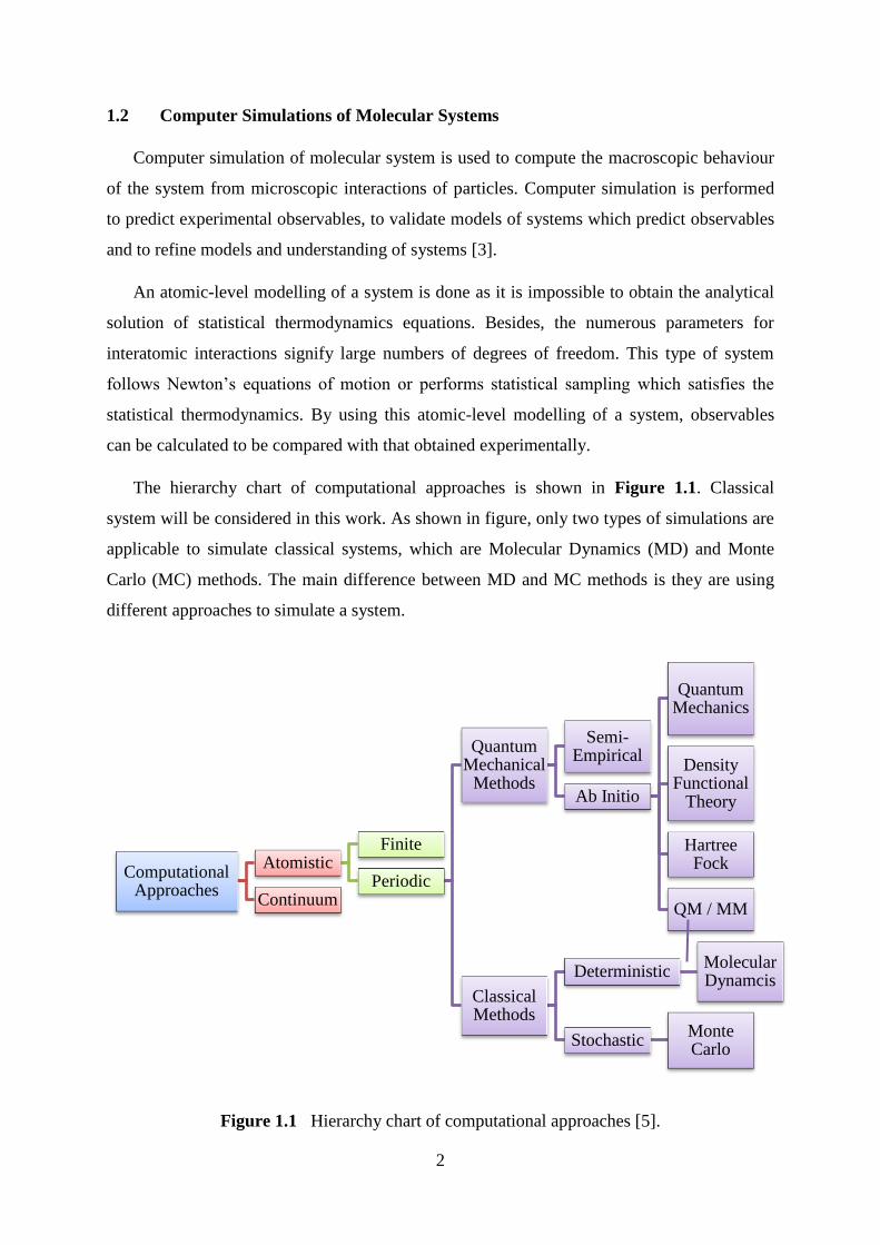
The hierarchy chart of computational approaches is shown in Figure 1.1. Classical

system will be considered in this work. As shown in figure, only two types of simulations are

applicable to simulate classical systems, which are Molecular Dynamics (MD) and Monte

Carlo (MC) methods. The main difference between MD and MC methods is they are using

different approaches to simulate a system.

Figure 1.1 Hierarchy chart of computational approaches [5].

Computational Approaches

Atomistic Finite

Periodic

Quantum Mechanical

Methods

Semi-Empirical

Ab Initio

Quantum Mechanics

Density Functional

Theory

Hartree Fock

QM / MM

Classical Methods

Deterministic Molecular Dynamcis

Stochastic Monte Carlo

Continuum

3

In MD, equations of motion are integrated to track the atoms. It is a deterministic

technique, which the subsequent time evaluation is completely determined when an initial set

of positions and velocities is given. On the other hand, MC method is a statistical method to

fill phase-space faster by moving the atoms randomly and system properties can be

statistically obtained.

In the last decade, there are many kinds of molecules have been simulated, including

proteins. MD has become an important tool for mechanical, chemical and biochemical

research. Also, MD simulation will be considered in this work.

There are two basic problems in the field of molecular modelling and simulation. First

one is to efficiently search the vast configuration space spanned by all possible molecular

conformations for the global low energy regions, which are populated by a molecular system

in thermal equilibrium. The other problem is the derivation of a sufficiently accurate

interaction energy function or force field for the molecular system of interest. Therefore, the

choice of assumptions, approximations and simplifications of the molecular model and

computational procedure are important. Their contributions to the overall inaccuracy are of

comparable size, without affecting significantly the property of interest [4].

There exists a variety of molecular models and force fields, differing in the accuracy by

which different physical quantities are modelled. When studying a molecular system by

computer simulation, there are three factors that are taken into consideration, as shown in

Figure 1.2, which are the property or quantity of interest of the molecular system, the

required accuracy of the properties and the estimation of available computing power.

Figure 1.2 Factors affecting choice of molecular model, force field and sample size [4].

Molecular model

force field sampling

Property or quantity of

interest

Required Accuracy

Available Computing

Power

4

1.3 Acknowledgement of Previous Work

In year 1967, Verlet studied the thermodynamical properties of LJ molecules [6]. It is

considered as one of the earliest computer simulation on classical fluids. In 1969, Hansen and

Verlet studied about phase transitions of the LJ system [7]. In 1979, Nicolas et al. [8] gave

the equations of state for MD calculation and this is later improved by by Johnson et al. [9] in

1993.

While Panagiotopoulos (1987, 1994, 2000) [10,11,12] and Smit (1996) [13] explored the

molecular simulation phase equilibria of fluids by using MC method, Matsumoto (1998) [14]

and Kai Gu et al. (2010) [15] exploring the MD of fluid phase change. In 2008, Bopp et al.

[16] reviewed both of these molecular simulation methods.

In this work, the main method employed will be the TQMD. It is based on the work of

Gelb and Müller (2002) [2] and Veracoechea and Müller (2005) [1], which are proposing an

effective method to simulate for fluid phase equilibria.

1.4 Scope and Content

The main scope of this work is to locate the phase equilibria of single component LJ fluid

by TQMD method. Although this method is capable to stimulate a complex system and can

be parallelized as mentioned by of Gelb and Müller (2002) [2] and Veracoechea and Müller

(2005) [1], the current code of TQMD method is sequential and limited to pure LJ fluid only.

The system is then simulated to further study about its properties.

Chapter 2 will be the literature reviews of this work, discussing the development of this

field, ranging from typical conventional methods to the more recent methods. The basic

theoretical foundation of MD method and theory behind methods employed in this work will

be discussed in Chapter 3.

Chapter 4 will discuss the methods employed in this work in more detail manner,

including the TQMD method. The theory and idea of TQMD method will be explored and

additional materials will be given. This section mainly based on the literature published by

Gelb and Müller (2002) [2] and Veracoechea and Müller (2005) [1].

5

Chapter 5 will discuss the results of simulation. Only major patterns, relationships and

generalization of the results will be discussed in this chapter, while full sets of results

including data and graphs will be included in the disc attached. Errors and deviation of results

from literature and standard results will be discussed in this chapter.

Chapter 6 includes the conclusion and recommendations for this work. General

conclusion is made based on the results obtained from simulation and thus verifying the

results from previous work. Recommendations about possible future extension of this

research are suggested.

6

CHAPTER 2

LITERATURE REVIEW

This chapter states the review from various literatures that have been published

throughout the years. This is important in providing knowledge and methods to be employed

in this work.

2.1 Classical Simulation of Lennard-Jones System

Verlet (1967) [6] had done one of the earliest computer simulations on classical fluids to

study the thermodynamics properties of LJ molecules. Verlet considered a system of 864

particles, enclosed in a cube of side L, with periodic boundary conditions interacting through

a two-body LJ potential. The equation of motion of a system has been integrated for various

values of the temperature and density to a fluid state. It appears that the LJ potential is a

satisfactory interaction as far as the equilibrium properties of argon are concerned. If the

system is replaced by xenon, the agreement would not be good. However, Verlet stated the

determination of critical constants is difficult due to the computational errors.

Two years later, together with Hansen, Verlet published a paper about the phase

transitions of the LJ system [7]. Monte Carlo (MC) computations have been performed in

order to determine the phase transitions of a system similar to the previous system. For the

liquid-gas transition, a method has been devised which forces the system to remain always

homogeneous. The equation of state of the liquid region was obtained for the reduced

temperature and by a standard MC calculation. In the gas region, the

equation of state can easily be obtained from virial expression. The coexistence curve for

argon is flatter in the critical region than the one deduced from machine computation, due to

the long-range density, which cannot be included in the MC calculation. At very low

temperatures, the transition density for the liquid branch shows a better agreement between

theory and experiment than that in the case of argon, due to the properties of dilute argon at

very low temperature is very poorly accounted for by the LJ potential. Results from an

approximate equation of state are good for LJ case. It is concluded that the phase transition of

LJ fluid can be calculated using methods where only homogeneous phase are considered.

7

2.2 Derived Equations of State

From Nicolas et al. (1979) [8], MD calculations of the pressure and configurational

energy of a LJ fluid are reported for 108 state conditions in the reduced density range

and reduced temperature range . Simulation results of

pressure and configurational energy, together with low density values calculated from the

virial series and value of second virial coefficients. These are used to derive an equation of

state for the LJ fluid that is valid over a wide range of temperatures and densities. The

equation of state used is a modified Benedict-Webb-Rubin (MBWR) equation having 33

constants. The virial series at low densities and computer simulation results at the higher

densities are used to derive an equation of state that is valid over a wide range of densities

and temperatures. Numerical convenience requires only a non-linear terms. The gas-liquid

coexistence curve calculated from the equation of state obtained was compared with the MC

data of existing literatures and the agreement is good. However, the equation of state are

interpolation expressions, and should not be used at state conditions outside of the region of

fit, otherwise significant errors are obtained if used to extrapolate to low temperatures.

Later, Johnson et al.(1993) [9] reviewed the existing simulation data and equations of

state for LJ fluid, and presented new simulation results for both the cut and shifted and the

full LJ potential. They presented the new parameters for MBWR equation of state used by

Nicolas et al. (1979) [8]. In contrast to previous equations, the new equation is accurate for

calculations of vapour-liquid equilibria. The equation accurately correlates pressures and

internal energies from the triple point to about 4.5 times the critical temperature over the

entire fluid range. An equation of state for the cut and shifted LJ fluid is presented. The

parameters are constrained to give a critical density and temperature. The equation of state is

not capable of fitting both the vapour-liquid region and high temperature region with

comparable accuracy. By comparing the predicted vapour-liquid equilibrium data, the

original Nicolas et al. parameters are quite accurate at low temperatures, but for reduced

temperature , the new parameters are significantly more accurate. Although the new

equation is more accurate than that of Nicolas et al. for vapour-liquid equilibrium

calculations, the accuracy of the new equation is somewhat lower for dense fluids at

temperatures greater than twice the critical.

8

2.3 Applications of Molecular Simulations

2.3.1 Monte Carlo Simulation

Smit (1996) [13] reviewed some applications of molecular simulations of phase equilibria.

Since the conventional simulations techniques require too much CPU-time, it is necessary to

simplify the models or to develop novel simulation techniques. In particular for phase

equilibrium calculations, the slow equilibration of complex fluids limits the range of

applications of molecular simulations. In the Gibbs-ensemble technique, simulations of the

vapour and liquid phase are carried out in parallel. MC moves allow the changes in volume

and number of particles. This ensures that the two boxes are in thermodynamic equilibrium

with each other. The coexistence densities can be determined directly from the two systems.

A model polar fluid with dispersive LJ interactions is considered instead of dipolar hard-

sphere fluid. At conditions where the coexistence curve is expected, chains of dipoles

aligning nose to tail are formed, which inhibit the phase separation. These simulation results

show that a minimum amount of dispersive energy is required to observe liquid-vapour

coexistence in a dipolar fluid. To conclude, dipolar hard-sphere fluid is not a good starting

point to develop a theory for real polar fluids. In real polar fluids the dispersive interactions

are essential to stabilize the liquid phase.

2.3.2 Molecular Dynamics Simulation

Matsumoto (1998) [14] applied MD simulation for various fluid systems to investigate

microscopic mechanisms of phase change. One of the works reviewed by his group was

evaporation–condensation dynamics of pure fluids under equilibrium condition. MD

simulation is done to investigate the dynamic behaviour of molecules under such conditions.

By analysing of molecular trajectories, dynamic behaviour of molecules near a liquid surface

is found to be classified into four categories, which are evaporation, condensation, self-

reflection and molecular exchange. Molecular exchange is important for cases such as

associating fluids and fluids at high temperatures. Another reviewed work is the evaporation–

condensation dynamics of pure fluids under non-equilibrium condition, which behaviour is

more complicated. Even with the liquid temperature given, there are two more control

parameters, which are the temperature and the density (or the pressure) of the vapour. The

9

situations include hot vapour condensation on cool liquid and evaporation into vacuum.

Similar method is applied to investigate gas absorption dynamics on liquid surfaces. For

carbon dioxide (CO2) gas absorption mechanism on water surface, the ions tend to avoid the

surface whereas CO2 molecules are strongly adsorbed on the surface where little ions exist.

Gu et al. (2010) [15] resolved the equilibrium structure of the finite, interphase interfacial

region that exists between a liquid film and a bulk vapour by MD simulation. Argon systems

are considered for a temperature range that extends below the melting point. Physically

consistent procedures are developed to define the boundaries between the interphase and the

liquid and vapour phases. The procedures involve counting of neighbouring molecules and

comparing the results with boundary criteria that permit the boundaries to be precisely

established. Definitions of both interphase boundaries are necessary to collect molecular mass

flux statistics for computation of interfacial mass transfer in MD simulations. The interphase

thicknesses determined from the new boundary criteria are more precise. By applying the

new criteria for interphase boundaries to MD computation of condensation and evaporation

coefficients produces result that, away from the melting point, the results are in better

agreement with transition state theory; near the melting point, transition theory

approximations are less valid.

2.4 Scope and Methods of Molecular Simulations

Bopp et al. (2008) [16] reviewed the basic tenets of MD and MC simulations,

highlighting their strengths and limitations. The fundamental ideal underlying all molecular

simulations are evaluated. It stated that MD and MC differ in the way the sample is generated.

While MD uses, as Boltzmann envisaged, classical Newtonian mechanics, MC rests on a

random walk procedure. In this article, two examples are simulated. The one interested is the

model of liquid-liquid interface. The systems consist of two types of LJ particles, the

miscibility of which is controlled by the radii of particles and the strengths of the interactions

between like and unlike particles. The dynamics will be influenced by the particle masses.

The system is initially prepared at a temperature above the critical point and then quenched to

start the process. Once the plane interfaces are formed, the system remains stable for the

duration of the simulation.

10

2.5 Temperature-Quench Molecular Dynamics Simulations

Gelb and Müller (2002) [2] presented a method to locate phase coexistence points using

MD simulations. This method can be used to locate vapour-liquid, liquid-liquid or solid-fluid

equilibria. The method is demonstrated on test systems of single component and binary LJ

fluids. When the system is suddenly set into an unstable state, it decomposes spinodally.

Since the cutoff radius is relatively large, the results follow expected equation of state of

Johnson et al. (1993) [9] for the full potential. It appears that TQMD is not limited to fluid

phase equilibria. If the final temperature is below the triple point, solid phases can nucleate

during the quenching process. To conclude, it is shown that TQMD gives correct results for

pure and multi-component vapour-liquid equilibria.

Two years later, Veracoechea and Müller (2004) [1] provided a more detailed account of

the TQMD method and particularly analyses the short-time phase separation behaviour of

fluids upon which it is based, as well as example applications to the vapour-liquid equilibria

of a pure LJ fluid, the liquid–liquid–vapour equilibria of a binary LJ system, and the

saturation densities of a long-chain alkane. The advantages of TQMD are shown from the

results obtained, which are similar, independent of the number of particles and simulation

time. The results obtained by this method are also shown to be of the same precision as those

obtained by GEMC or volume expansion molecular dynamics (VEMD).

11

CHAPTER 3

THEORY

This chapter details the theory behind MD simulation. The following section provides an

overall idea of the molecular simulation and the subsequent sections detail the essential

theory of MD, which will be useful in computing later.

3.1 Molecular Simulation

The fundamental idea underlying all molecular simulations is simple and follows directly

from Boltzmann‟s thinking about the “thermodynamic ensembles”. A simulation is defined as

a sufficient number of microscopic configurations, or states, are constructed, compatible with

the macroscopic thermodynamic constraints of the system under consideration, which are

temperature, density and etc. Secondly, the configurations are compatible with the

intermolecular or interatomic interactions in the system. Another idea is an evaluation, which

statistical tools are used to compute averages over these configurations.

MD and MC are two simulation methods alluded to above criteria, which differ in way

the sample is generated. MD uses classical Newtonian mechanics while MC rests on a

random walk procedure. In both cases, the model describing the interactions between the

particles in the system is the critical input to any simulation. Overall idea of molecular

simulation is summarized in Figure 3.1.

The two methods do not yield the same amount of information about the system. MD,

being based on Newton‟s equation, samples the “phase space” of the system, which contains

all positions and all momenta of all particles in the system at a given time . The sample of

the ensemble constructed thus contains information about the time evolution of the system.

MC samples „„configurational space”, concerning only information about the particle

positions.

12

Figure 3.1 Schematic view of molecular simulations [16].

3.2 Lennard-Jones Potential

The LJ potential is a mathematically simple model that describes the interaction between

a pair of neutral atoms or molecules. The LJ potential is a relatively good and universal

approximation. It is particularly accurate for noble gas atoms and is a good approximation at

long and short distances for neutral atoms and molecules.

The LJ potential is expressed as [3] :

( ) [(

)

(

)

] (3.1)

where is the separation of the particles, while and are constants that set the energy and

distance scales associated with the interaction respectively. In fact, is given by the depth of

the potential well while is the finite distance at which the interparticle potential is zero.

This function is illustrated in Figure 3.2.

13

Figure 3.2 Lennard-Jones Potential [17]

The physical origin of LJ potential is related to the Pauli principle. For large separations,

the interaction is due to the Van der Waals force, which is a weak attraction arising from the

transient electric dipole moments of the two atoms. This potential varies as and is

attractive. When the atoms get close together, the electronic clouds surrounding the atoms

start to overlap. The energy of the system increases abruptly due to the exchange interaction.

This potential varies as and is repulsive.

3.3 Reduced Units

In simulations, it is often convenient to express in reduced units. This means that a

convenient unit of energy, length and mass are chosen and then all other quantities are

expressed in terms of these basic units. The reduced units are usually denoted by superscript

of *. Table 3.1 illustrates the common reduced units used in calculations.

The reduced form for the LJ potential is given by [18] :

( ) [(

)

(

)

] (3.2)

14

With these conventions, some reduced units like potential energy, pressure, density amd

temperature can be defined, which are illustrated in Table 3.1 as well.

Table 3.1 Reduced units for molecular simulation [18].

Quantities Units Reduced Units

Length, L Energy, U Mass, m Time, t √ ( √ )

Temperature, T ( )

Pressure, P ( ) Density,

It is convenient to introduce reduced units. The most important reason is that many

combinations of , , and all correspond to the same state in reduced units, which is the

law of corresponding states. In reduced units, almost all quantities of interest are of order 1.

Hence, another reason is that error can be detected easily in the simulation.

Simulation results obtained in reduced units can be translated back into real units. For

example, the results of a simulation on a LJ model at certain and can be compared with

experimental data for argon, by using the translation given in Table 3.2 to convert the

simulation parameters to real SI units.

Table 3.2 Translation of reduced units to real units for LJ argon [18]

Quantity Reduced Units Real Units

Temperature

Density

Time Pressure

15

3.4 Periodic Boundary Condition

For presently available computers, the systems are limited to be containing a relatively

small number of atoms. In small systems, the collisions with the walls can be a significant

fraction of the total number of collisions, while in real system; the behavior would be

dominated by collisions with other particles.

In order to simulate bulk phases, it is essential to choose boundary conditions that mimic

the presence of an infinite bulk surrounding the -particle model system. This is usually done

by applying periodic boundary conditions. The volume containing the particles is treated as

the primitive cell of an infinite periodic lattice of identical cells. A given particle now

interacts with all other particles in the infinite periodic system, that is, all other particles in

the same periodic cell and all particles in all other cells, including its own periodic image. A

system with periodic boundary conditions is shown schematically in Figure 3.3.

Figure 3.3 Schematic representation of periodic boundary conditions [18]

There are two consequences of this periodicity. The first is that an atom that leaves the

simulation region through a particular bounding face immediately reenters the region through

the opposite face, as shown in Figure 3.4. The second is that minimum separation rule, which

acts as a precautionary step when considering relative positions of the particles. For the

equations of motion to be consistent, particles should only be allowed to interact once. Hence,

the smaller separation is used to calculate the magnitude and direction of the force, as shown

in Figure 3.5.

16

Figure 3.4 Periodic boundary conditions for a molecular dynamics simulation using an

box. The arrows denote atoms and their velocities. [3]

Figure 3.5 Shortest distance between particles in a system with periodic boundary condition.

[19]

17

3.5 Molecular Dynamics Simulation

3.5.1 Classical Approach

Consider a simulation of a collection of atoms, where each atom is treated as a simple

structureless particle with wavelength that is much smaller than the particle separation, as in

noble gases. This type of system allows to be applied with classical treatment. In the classical

mechanics approach to MD simulations, molecules or atoms are treated as classical objects.

The laws of classical mechanics define the dynamics of the system. In MD simulation,

Newton‟s equations of motion are integrated numerically to study behavior of system over

time.

3.5.2 Newtonian Mechanics

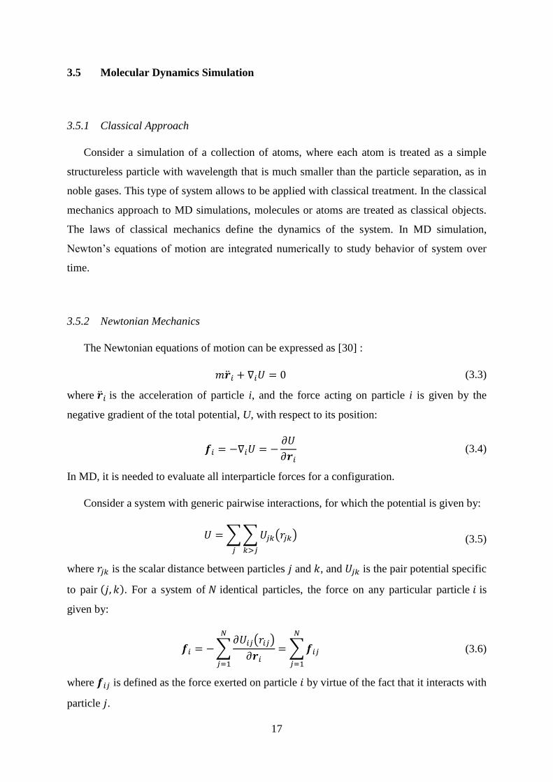
The Newtonian equations of motion can be expressed as [30] :

(3.3)

where is the acceleration of particle i, and the force acting on particle i is given by the

negative gradient of the total potential, U, with respect to its position:

(3.4)

In MD, it is needed to evaluate all interparticle forces for a configuration.

Consider a system with generic pairwise interactions, for which the potential is given by:

∑∑ ( )

(3.5)

where is the scalar distance between particles and , and is the pair potential specific

to pair ( ). For a system of identical particles, the force on any particular particle is

given by:

∑ ( )

∑

(3.6)

where is defined as the force exerted on particle by virtue of the fact that it interacts with

particle .

18

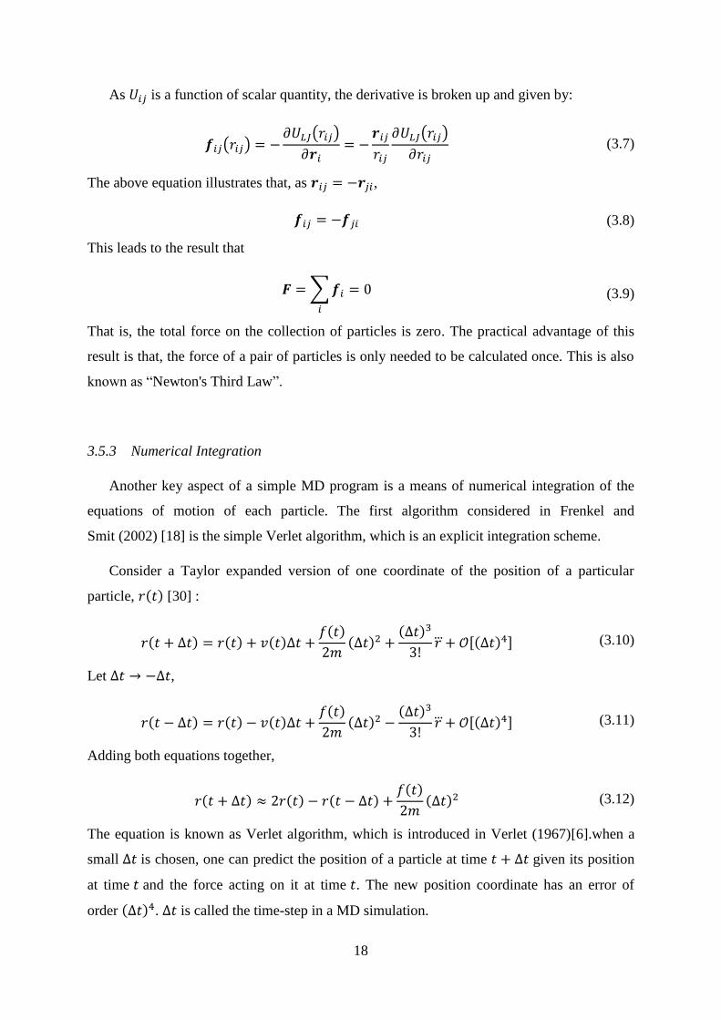
As is a function of scalar quantity, the derivative is broken up and given by:

( ) ( )

( )

(3.7)

The above equation illustrates that, as ,

(3.8)

This leads to the result that

∑

(3.9)

That is, the total force on the collection of particles is zero. The practical advantage of this

result is that, the force of a pair of particles is only needed to be calculated once. This is also

known as “Newton's Third Law”.

3.5.3 Numerical Integration

Another key aspect of a simple MD program is a means of numerical integration of the

equations of motion of each particle. The first algorithm considered in Frenkel and

Smit (2002) [18] is the simple Verlet algorithm, which is an explicit integration scheme.

Consider a Taylor expanded version of one coordinate of the position of a particular

particle, ( ) [30] :

( ) ( ) ( ) ( )

( )

( )

[( ) ] (3.10)

Let ,

( ) ( ) ( ) ( )

( )

( )

[( ) ] (3.11)

Adding both equations together,

( ) ( ) ( ) ( )

( ) (3.12)

The equation is known as Verlet algorithm, which is introduced in Verlet (1967)[6].when a

small is chosen, one can predict the position of a particle at time given its position

at time and the force acting on it at time . The new position coordinate has an error of

order ( ) . is called the time-step in a MD simulation.

19

A system obeying Newtonian mechanics conserves total energy. For a dynamical system

obeying Newtonian mechanics, the configurations generated by integration are members of

the microcanonical ensemble; that is, an ensemble of configurations for which number of

particles, volume and energy of the system ( ) are constant, constrained to a subvolume

in phase space.

When the Verlet algorithm is used to integrate Newtonian equations of motion, the total

energy of the system is conserved to within a finite error, so long as is small enough.

Although total energy is the sum of potential energy and kinetic energy, velocities are not

necessary in Verlet algorithm. They can be easily generated provided that one stores previous,

current, and next-time-step positions in implementing the algorithm:

( ) ( ) ( )

[( ) ] (3.13)

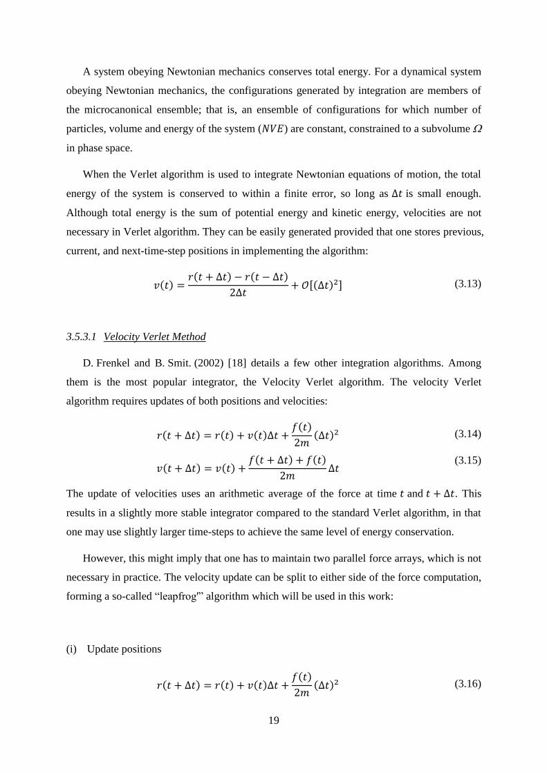
3.5.3.1 Velocity Verlet Method

D. Frenkel and B. Smit. (2002) [18] details a few other integration algorithms. Among

them is the most popular integrator, the Velocity Verlet algorithm. The velocity Verlet

algorithm requires updates of both positions and velocities:

( ) ( ) ( ) ( )

( ) (3.14)

( ) ( ) ( ) ( )

(3.15)

The update of velocities uses an arithmetic average of the force at time and . This

results in a slightly more stable integrator compared to the standard Verlet algorithm, in that

one may use slightly larger time-steps to achieve the same level of energy conservation.

However, this might imply that one has to maintain two parallel force arrays, which is not

necessary in practice. The velocity update can be split to either side of the force computation,

forming a so-called “leapfrog'” algorithm which will be used in this work:

(i) Update positions

( ) ( ) ( ) ( )

( ) (3.16)

20

(ii) Half-update velocities

(

) ( )

( )

(3.17)

(iii) Compute forces

( ) ( ) (3.18)

(iv) Half update velocities

( ) (

)

( )

(3.19)

3.5.3.2 Truncation of Interactions

Consider a simulation of a system with short-range interactions. In this context, short-

ranged means that the total potential energy of a given particle is dominated by interactions

with neighbouring particles that are closer than some cutoff distance, . The error that results

when the interactions with particles at larger distances are ignored can be made arbitrarily

small by choosing sufficiently large.

Truncation of a pair potential is an important idea to understand. The major point is that

the cutoff must be spherically symmetric; that is, interactions beyond a box length in each

direction cannot be simply cut off. This is due to the consequence in a directional bias in the

interaction range of the potential. Hence, a hard cutoff radius, , is required and should be

less than half a box length. For distance larger than , if the intermolecular potential is not

zero, correction terms for energy and pressure must be employed to reduce the systematic

error in the simulation.

According to Frenkel and Smit. (2002) [18], for LJ potential, the potential and pressure

tail correction terms are respectively given by:

[

(

)

(

)

] (3.20)

[

(

)

(

)

] (3.21)

21

There are several ways to truncate potentials on a simulation. Two of the often used

methods are discussed here [18] :

(i) Simple Truncation

The simplest method to truncate potentials is to ignore all interaction beyond , the

potential that is simulated is

( ) { ( )

(3.22)

This may result in an error in the estimation of the potential energy of the true LJ

potential. Besides, as the potential changes discontinuously at , a truncated potential is

not particularly suitable for a MD simulation. However, it can be used in MC simulations.

(ii) Truncation and Shift

It is common to be used in MD simulations; also it is employed in this work. The

potential is truncated and shifted, such that the potential vanishes at the cutoff radius:

( ) { ( ) ( )

(3.23)

Since there are no discontinuities in the intermolecular potential, there is no impulsive

correction to the pressure. It has the benefit that the intermolecular forces are always

finite. This is important as impulsive forces cannot be handled in molecular dynamics

algorithms to integrate the equations of motion that are based on a Taylor expansion of

the particle positions.

3.5.3.3 Instantaneous Temperature

According to equipartition theorem of energy, the working definition of instantaneous

temperature, T, is given by the following. However, for a microcanonical system, the actual

temperature is time average.

∑ | |

(3.24)

where is the Boltzmann constant.

22

3.5.3.4 Instantaneous Pressure

The working definition of instantaneous pressure, P, is given by:

(3.25)

where V is the volume of system and is the virial:

∑ ( )

(3.26)

3.5.3.5 Berendsen Thermostat

The scale factor for thermostat, , is given by:

[

( )]

(3.27)

where is the target temperature, is the integration time step, and is a constant called

the rise time of the thermostat. It describes the strength of the coupling of the system to a

hypothetical heat bath. The larger the , the longer it takes to achieve a given after an

instantaneous change from some previous .

3.5.3.6 Berendsen Barostat

Consider a cubic system, where . The Berendsen barostat uses a scale factor, ,

which is a function of , to scale lengths in the system :

(3.28)

(3.29)

While scale factor for barostat, , is given by:

[

( )]

(3.30)

where is the initial pressure, is the integration time-step, and is a constant called the

"rise time" of the barostat.

23

3.5.3.7 Radial Distribution Function

Radial distribution function (RDF), ( ), gives the probability of finding a particle in the

distance from another particle. The RDF is a useful tool to describe the structure of a

system. In systems, where there is continual movement of the atoms and a single snapshot of

the system shows only the instantaneous disorder, it is extremely useful to deal with the

average structure.

To calculate the RDF from a simulation, the neighbours around each atom or molecule

are sorted into distance bins, as shown in Figure 3.6. The number of neighbours in each bin

is averaged over the entire simulation. First, choose an atom in the system and draw around it

a series of concentric spheres, set at a small fixed distance, . At regular intervals a snapshot

of the system is taken and the number of atoms found in each shell is counted and stored. At

the end of the simulation, the average number of atoms in each shell is calculated. This is

then divided by the volume of each shell and the average density of atoms in the system.

Figure 3.6 Radial distribution function [20].

The RDF is usually plotted as a function of the interatomic separation . A peak indicates

a particularly favoured separation distance for the neighbours to a given particle. Thus, RDF

reveals details about the atomic structure of the system being simulated. The first peak

corresponds to the nearest neighbour shell, the second peak to the second nearest neighbour

shell, etc.

24

Figure 3.7 shows typical radial distribution plots of argon at different temperature. At

short separations (small ), the radial distribution function is zero. This indicates the effective

width of the atoms, since they cannot approach any more closely. A number of obvious peaks

appear which indicate that the atoms pack around each other in neighbour shells. At high

temperature the peaks are broad, indicating thermal motion, while at low temperature they are

sharp.

Figure 3.7 Typical radial distribution plots of argon at different temperature [21].

3.5.3.8 Ideal and Real Gases

In an ideal gas, the only contribution to its energy is the kinetic energy of the particles.

On the other hand, if the particles in a real gas are close enough, they will interact and

potential energy is contributed to the energy. At low temperatures or high pressures, real

gases deviate significantly from ideal gas behaviour.

Deviations from ideality can be described by the compression factor, , which is known

as the compressibility. When a gas obeys ideal gas law, the compression factor equals 1.

Compression factor, , is given by:

(3.31)

25

3.5.4 Summary

According to Giordano and Nakanishi (2006) [3], for any MD simulation, the important

procedure can be expressed as followings:

1. Parameters that specify the conditions of the run are read in. For example, the initial

temperature, number of particles, density, and time step, etc.

2. The system is initialized by assigning initial positions and velocities

3. Forces on all particles are computed.

4. Newton‟s equations of motion are integrated by using suitable integrator. This step

and the previous one make up the core of the simulation. They are repeated until the

time evolution of the system is computed for the desired length of time.

5. After completion of the central loop, the averages of measured quantities are

computed and output. Then, the process is stopped.

Figure 3.8 Molecular dynamics process flow chart.

26

CHAPTER 4

METHODOLOGY

This chapter details the MD simulation method that has been used. The following section

provides an overview of the method and the subsequent sections detail the main methods for

simulating the system and computing statistics.

4.1 Overview

4.1.1 Temperature-Quench Molecular Dynamics

There are several parameters that need to be initialized at the beginning of the simulation.

In this work, these parameters are set in reduced units. First of all, the number of particles, ,

is set to be 32,000. The overall reduced density of particle, , is set to 0.328. With these

parameters, volume of the system, , which is a cubic box containing the particles, can be

calculated by . The reduced cutoff radius, , where the potential is truncated, is set to be

5.0. The system is set to face-centred cubic (FCC) lattice, according to the algorithm used by

Thijssen in his example code for his book [28]. The velocity of each particle is then assigned

according to the Boltzmann distribution function after setting the initial temperature.

The initial temperature of the system, in reduced unit, is set to be , the system is

then quenched to desired reduced temperatures of 0.7, 0.8, 0.9, 1.0, 1.1, 1.2. The time step for

the simulation, , is chosen to be 0.004. Two simulations are done in this work, each with

different total simulation steps. The first one, which has total simulation steps of 120,000, is

allowed to be equilibrated after 7,000 steps. The later comparisons in Chapter 5 will be based

on this configuration. The second simulation with total of 330,000 steps is allowed to be

equilibrated after 130,000 steps of simulation. When the system is allowed to be equilibrated,

the system will be settled down to its stable state. Neighbor cell subdivision algorithm [29] is

used to compute the interactions instead of all-pairs method, as it increases the efficiency of

force calculation.

The simulation is carried out as a constant-temperature, constant-volume ensemble

( ), also referred to as the canonical ensemble. The ensemble is obtained by controlling

27

the temperature through Berendsen thermostat. The system initially at a temperature, which is

much higher than the critical temperature obtained from literature. The system is then

quenched to a desired temperature. The sudden drop of temperature results in the particles

separate into two distinct phases as the system becomes unstable. The particles at the

interface of both separated phases are detected by interface detection algorithm. They are

isolated out for further analysis. Bulk liquid and gas phases are obtained and density of each

phase is computed. Critical point of phase diagram is obtained by using the law of rectilinear

diameter [1]. It is later compared and discussed with the value from existing literature. The

simulation is repeated for total of 330,000 steps of simulation. Both set of results are

compared and discussed.

4.1.2 Study of Properties of Lennard-Jones Fluid

LJ fluid system are simulated under various state point of the phase diagram by using

Mathematica software. Since the simulation is done observe the variation in certain

observables as it goes through phase diagram, the number of particles can be reduced to be

256. Two simulations are carried out with different ensemble, that is, one with ensemble

by using Berendsen thermostat and another with constant-temperature, constant-pressure

ensemble ( ).

4.2 Temperature-Quench Molecular Dynamics Simulations

4.2.1 Overall Process Flow

Temperature-quench molecular dynamics (TQMD) simulation is a method which locating

fluid phase coexistence through single canonical simulation in which the temperature is

changed in a single time step, which is known as quenching, At this unstable state, the single

phase, which is first equilibrated before quenching, is spontaneously separated into domains

of coexisting phases. Phase equilibrium properties can be observed by analyzing these

coexisting domains in terms of local densities, compositions, or other order parameter. This

method can be used to locate vapor–liquid, liquid–liquid or solid–fluid equilibria. The overall

process can be summarized as shown in Figure 4.1.

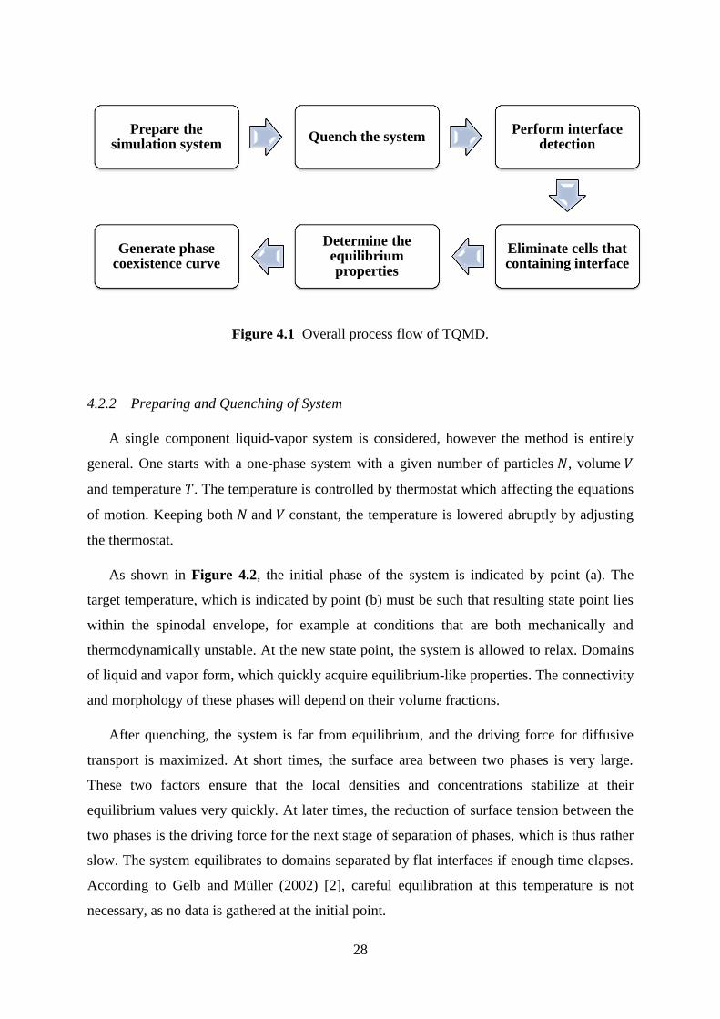
28

Figure 4.1 Overall process flow of TQMD.

4.2.2 Preparing and Quenching of System

A single component liquid-vapor system is considered, however the method is entirely

general. One starts with a one-phase system with a given number of particles , volume

and temperature . The temperature is controlled by thermostat which affecting the equations

of motion. Keeping both and constant, the temperature is lowered abruptly by adjusting

the thermostat.

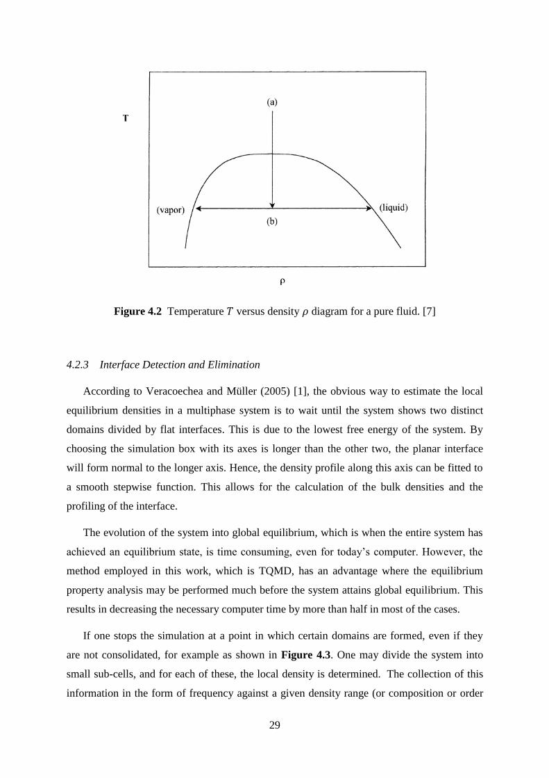
As shown in Figure 4.2, the initial phase of the system is indicated by point (a). The

target temperature, which is indicated by point (b) must be such that resulting state point lies

within the spinodal envelope, for example at conditions that are both mechanically and

thermodynamically unstable. At the new state point, the system is allowed to relax. Domains

of liquid and vapor form, which quickly acquire equilibrium-like properties. The connectivity

and morphology of these phases will depend on their volume fractions.

After quenching, the system is far from equilibrium, and the driving force for diffusive

transport is maximized. At short times, the surface area between two phases is very large.

These two factors ensure that the local densities and concentrations stabilize at their

equilibrium values very quickly. At later times, the reduction of surface tension between the

two phases is the driving force for the next stage of separation of phases, which is thus rather

slow. The system equilibrates to domains separated by flat interfaces if enough time elapses.

According to Gelb and Müller (2002) [2], careful equilibration at this temperature is not

necessary, as no data is gathered at the initial point.

Prepare the simulation system

Quench the system Perform interface

detection

Eliminate cells that containing interface

Determine the equilibrium properties

Generate phase coexistence curve

29

Figure 4.2 Temperature versus density diagram for a pure fluid. [7]

4.2.3 Interface Detection and Elimination

According to Veracoechea and Müller (2005) [1], the obvious way to estimate the local

equilibrium densities in a multiphase system is to wait until the system shows two distinct

domains divided by flat interfaces. This is due to the lowest free energy of the system. By

choosing the simulation box with its axes is longer than the other two, the planar interface

will form normal to the longer axis. Hence, the density profile along this axis can be fitted to

a smooth stepwise function. This allows for the calculation of the bulk densities and the

profiling of the interface.

The evolution of the system into global equilibrium, which is when the entire system has

achieved an equilibrium state, is time consuming, even for today‟s computer. However, the

method employed in this work, which is TQMD, has an advantage where the equilibrium

property analysis may be performed much before the system attains global equilibrium. This

results in decreasing the necessary computer time by more than half in most of the cases.

If one stops the simulation at a point in which certain domains are formed, even if they

are not consolidated, for example as shown in Figure 4.3. One may divide the system into

small sub-cells, and for each of these, the local density is determined. The collection of this

information in the form of frequency against a given density range (or composition or order

30

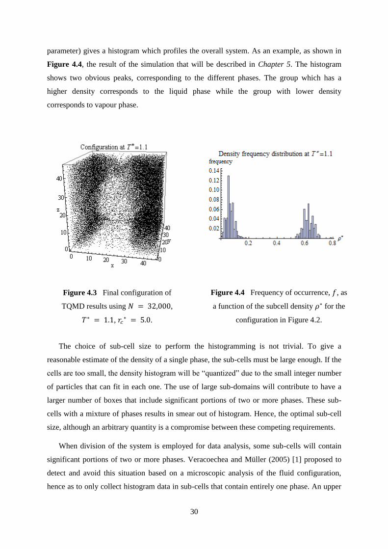
parameter) gives a histogram which profiles the overall system. As an example, as shown in

Figure 4.4, the result of the simulation that will be described in Chapter 5. The histogram

shows two obvious peaks, corresponding to the different phases. The group which has a

higher density corresponds to the liquid phase while the group with lower density

corresponds to vapour phase.

The choice of sub-cell size to perform the histogramming is not trivial. To give a

reasonable estimate of the density of a single phase, the sub-cells must be large enough. If the

cells are too small, the density histogram will be “quantized” due to the small integer number

of particles that can fit in each one. The use of large sub-domains will contribute to have a

larger number of boxes that include significant portions of two or more phases. These sub-

cells with a mixture of phases results in smear out of histogram. Hence, the optimal sub-cell

size, although an arbitrary quantity is a compromise between these competing requirements.

When division of the system is employed for data analysis, some sub-cells will contain

significant portions of two or more phases. Veracoechea and Müller (2005) [1] proposed to

detect and avoid this situation based on a microscopic analysis of the fluid configuration,

hence as to only collect histogram data in sub-cells that contain entirely one phase. An upper

Figure 4.4 Frequency of occurrence, 𝑓, as

a function of the subcell density 𝜌 for the

configuration in Figure 4.2.

Figure 4.3 Final configuration of

TQMD results using 𝑁 ,

𝑇 , 𝑟𝑐 .

31

(CNU) and lower (CNL) bound coordination number are defined for which a molecule is

considered as a member of each phase.

The coordination number is defined arbitrarily as the number of neighbours a molecule

will have within a fixed radius, which is in this work. Particles that are “in” an interface

between two phases have coordination numbers reflecting the interfacial region; for example,

in the case of vapour-liquid equilibria, they have neighbours lesser than particles in vapour

phase, and greater than particles in the vapour phase. For this case, sub-cells that contain

more than 15% “interfacial” particles are then excluded from the histogram count. In all cases,

A rough estimate of the density or concentration differences between the two phases is the

only need. It is easily obtained through computer graphics visualizations of the quenched

system.

4.2.4 Determination of Equilibrium Properties

One may attempt choose the maximum shown in the histograms to obtain the

corresponding phase densities. However, this method is quantitatively poor due to the

quantization of the histogram, and thus the accuracy of the estimation will be of the order of

magnitude of the bin size of the histograms. According to Veracoechea and Müller (2005) [1],

if one assumes that the maximum frequency of occurrence to correspond to the mean density,

the results are erroneous. However, in all cases, correct result can be obtained if either a

maximum likelihood analysis or a weighted average of the histograms is used. In this work,

the results are obtained by using the weighted average of histograms method.

32

CHAPTER 5

RESULTS AND DISCUSSION

This chapter discusses the results obtained in MD simulation. The following sections

provides discussion on results obtained using TQMD and comparisons these results with

results obtained in existing literatures. The subsequent sections detail discussion on the

relationships between various parameters to study the properties of LJ fluid.

5.1 Temperature-Quench Molecular Dynamics Simulations

5.1.1 Vapour-Liquid Coexistence Curve

The vapour liquid coexistence curve for first simulation is plotted as shown in Figure 5.1.

From the figure, the purple points are estimated using the law of rectilinear diameter and

scaled density temperature relation with an Ising exponent of 0.32 [1]. The blue points are

results obtained from simulation. The red point indicates the critical point. It is found that the

critical temperature obtained is while the critical density is

0.0013.

Figure 5.1 Vapour liquid coexistence curve for LJ system with 32,000 particles in 120,000-

step-simulation with .

33

The phase coexistence curve is generated based on the frequency distribution of density

of system at various temperature, as shown in Figure 5.2. As discussed in Section 4.2.2, the

system is divided into small sub-cells, and for each of these, the local density is determined.

From the figure, there are two peaks in each histogram. Each of these peaks indicates the bulk

and gas phase. The region between these phases is excluded using interface detection

algorithm.

Figure 5.2 Frequency distribution of density at various temperatures, using 32,000 particles

with 120,000 time steps at different temperature.

34

5.1.2 Comparison with TQMD by Müller

Müller (2005) [1] obtained the critical point at with

. By comparing with the simulation results obtained, which are

and 0.0013, the statistical error exists in this simulation is larger than that

obtained by Müller.

This may due to the different thermostat and integrating algorithm used in the simulation.

In this work, thermostat used is known as Berendsen thermostat, while a more superior

thermostat which is Nosé-Hoover thermostat is used by Müller. Velocity Verlet algorithm is

used in this work, whereas 5th-order Gear predictor–corrector algorithm is used by Müller.

Berendsen thermostat works by scaling the velocities to obtain an exponential relaxation

of the temperature to target temperature. To maintain the temperature, the system is coupled

to an external heat bath. This method gives an exponential decay of the system towards the

desired temperature. However, it does not represent a true canonical ensemble as the

thermostat suppresses fluctuations of the kinetic energy of the system.

Nosé-Hoover thermostat is based on additional degree of freedom coupled to the physical

system acts as heat bath. It uses extended-Lagrangian equations of motion, which are are

smooth, deterministic and time-reversible. It acts like isokinetic algorithm, but it permits

fluctuations in the momentum temperature. This thermostat correctly samples canonical

ensemble for both momentum and configurations.

The Gear algorithm can achieve a higher degree of energy conservation than the Verlet

algorithm with a longer time step. Gear algorithm might increase in memory requirement and

complexity. However, the Gear algorithm has an enormous advantage over the velocity

Verlet algorithm: it requires only one calculation of the interaction force per time step, while

the velocity Verlet algorithm makes two calls to that function at each update. One can readily

construct a given configuration and time step such that the velocity Verlet algorithm will gain

energy while the Gear algorithm remains stable.

35

5.1.3 Comparison with GEMC by Müller

Results obtained from first simulation for each temperature are given in Table 5.1, where

they can be quantitatively compared to those obtained from GEMC. The GEMC runs on

4,000 particle systems, discarding configurations and averaging over

configurations. Both sets of data made good and acceptable agreement with one another.

Note that, the error of critical point by TQMD calculated by Mathematica, uses error as

weight in model fitting.

The lowest temperature point, where , was not reported for GEMC. This is due

to the poor statistics obtained caused by the failure of the particle insertion step to accurately

sample the high density of the corresponding liquid.

According to Müller, this system size is far larger than that needed for this particular

application; it is the order of magnitude that is needed for studies of multicomponent

mixtures, asymmetric and/or multiphase fluids. The number of particles simulated only

affects the stability of the approach towards the expected equilibrium values. The smaller

system size shows greater fluctuations than that of larger system size. In fact, both systems

behave similarly in terms of the number of time steps required to obtain a suitable density

estimate. After roughly 100,000 time steps, the density analysis will give the same resulting

value. This confirms the fact that, for the accurate determination of equilibrium properties,

the cluster size needed is small.

Table 5.1 Saturated vapor density, , liquid density,

, as a function of temperature for

a pure LJ cut and shifted ( ) potential as obtained from 120,000-step-TQMD and

GEMC.

TQMD GEMC

T*

0.7 0.00259387(4) 0.833345 (31)

0.8 0.00662778(7) 0.788268(31) 0.0071(5) 0.79(1)

0.9 0.0178247(13) 0.742599(32) 0.016(2) 0.74(2)

1.0 0.0380098(19) 0.688202(32) 0.034(2) 0.69(1)

1.1 0.0664918(28) 0.622972(38) 0.063(6) 0.625(10)

1.2 0.118373(73) 0.543659(81) 0.117(7) 0.54(1)

1.2896(7) 0.313224(1) 0.313224(1)

Data for GEMC is taken from [1]. 0.123(4) corresponds to

36

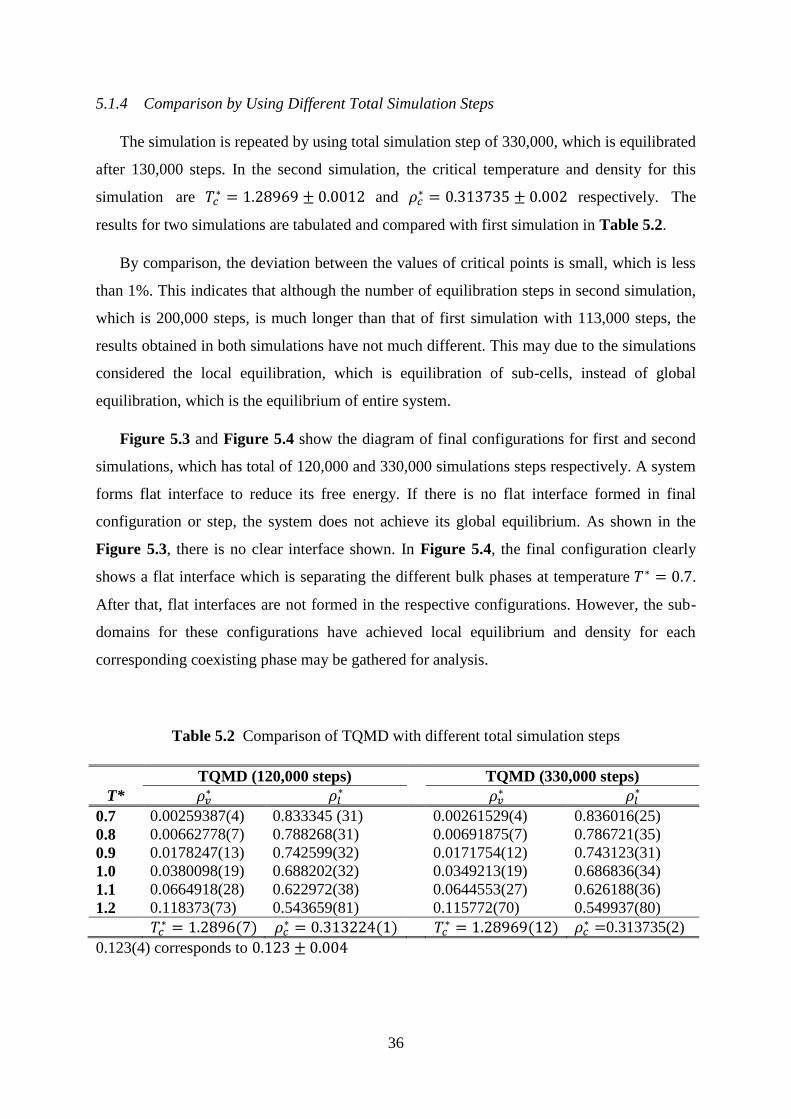
5.1.4 Comparison by Using Different Total Simulation Steps

The simulation is repeated by using total simulation step of 330,000, which is equilibrated

after 130,000 steps. In the second simulation, the critical temperature and density for this

simulation are and

respectively. The

results for two simulations are tabulated and compared with first simulation in Table 5.2.

By comparison, the deviation between the values of critical points is small, which is less

than 1%. This indicates that although the number of equilibration steps in second simulation,

which is 200,000 steps, is much longer than that of first simulation with 113,000 steps, the

results obtained in both simulations have not much different. This may due to the simulations

considered the local equilibration, which is equilibration of sub-cells, instead of global

equilibration, which is the equilibrium of entire system.

Figure 5.3 and Figure 5.4 show the diagram of final configurations for first and second

simulations, which has total of 120,000 and 330,000 simulations steps respectively. A system

forms flat interface to reduce its free energy. If there is no flat interface formed in final

configuration or step, the system does not achieve its global equilibrium. As shown in the

Figure 5.3, there is no clear interface shown. In Figure 5.4, the final configuration clearly

shows a flat interface which is separating the different bulk phases at temperature .

After that, flat interfaces are not formed in the respective configurations. However, the sub-

domains for these configurations have achieved local equilibrium and density for each

corresponding coexisting phase may be gathered for analysis.

Table 5.2 Comparison of TQMD with different total simulation steps

TQMD (120,000 steps) TQMD (330,000 steps)

T*

0.7 0.00259387(4) 0.833345 (31) 0.00261529(4) 0.836016(25)

0.8 0.00662778(7) 0.788268(31) 0.00691875(7) 0.786721(35)

0.9 0.0178247(13) 0.742599(32) 0.0171754(12) 0.743123(31)

1.0 0.0380098(19) 0.688202(32) 0.0349213(19) 0.686836(34)

1.1 0.0664918(28) 0.622972(38) 0.0644553(27) 0.626188(36)

1.2 0.118373(73) 0.543659(81) 0.115772(70) 0.549937(80)

( )

( ) ( )

0.313735(2)

0.123(4) corresponds to

37

Figure 5.3 Final configuration of TQMD using 120,000 time steps at different temperature.

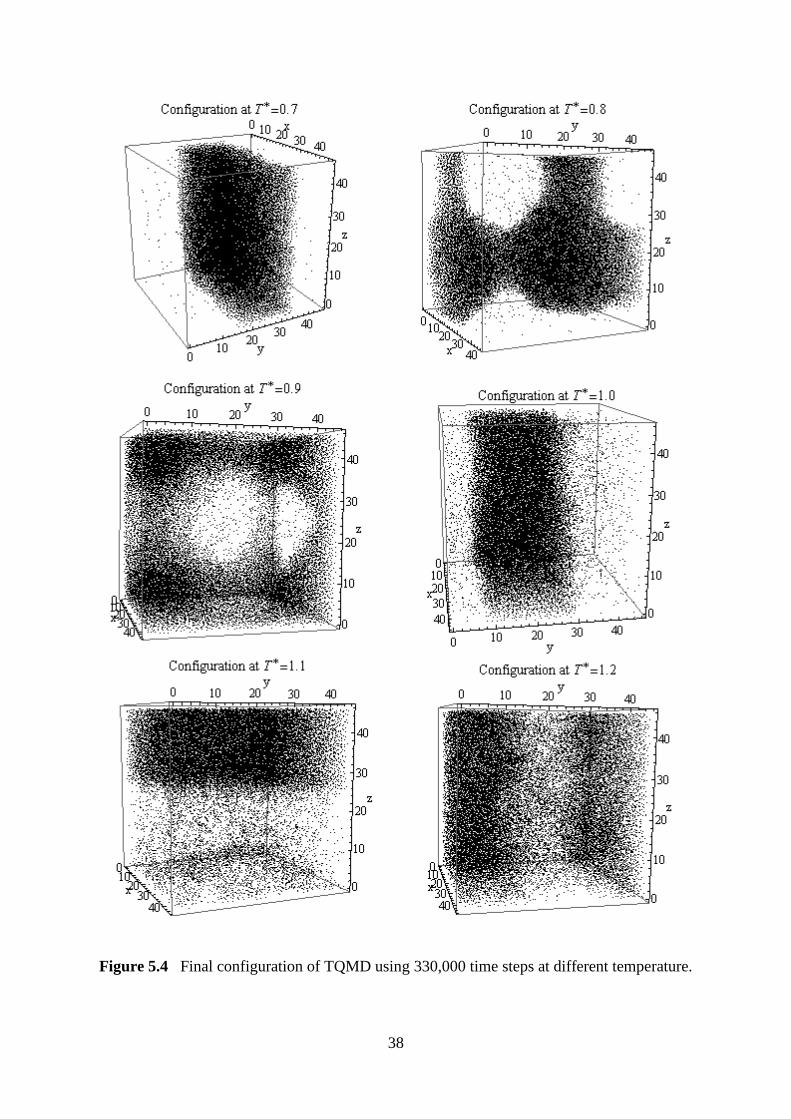
38

Figure 5.4 Final configuration of TQMD using 330,000 time steps at different temperature.

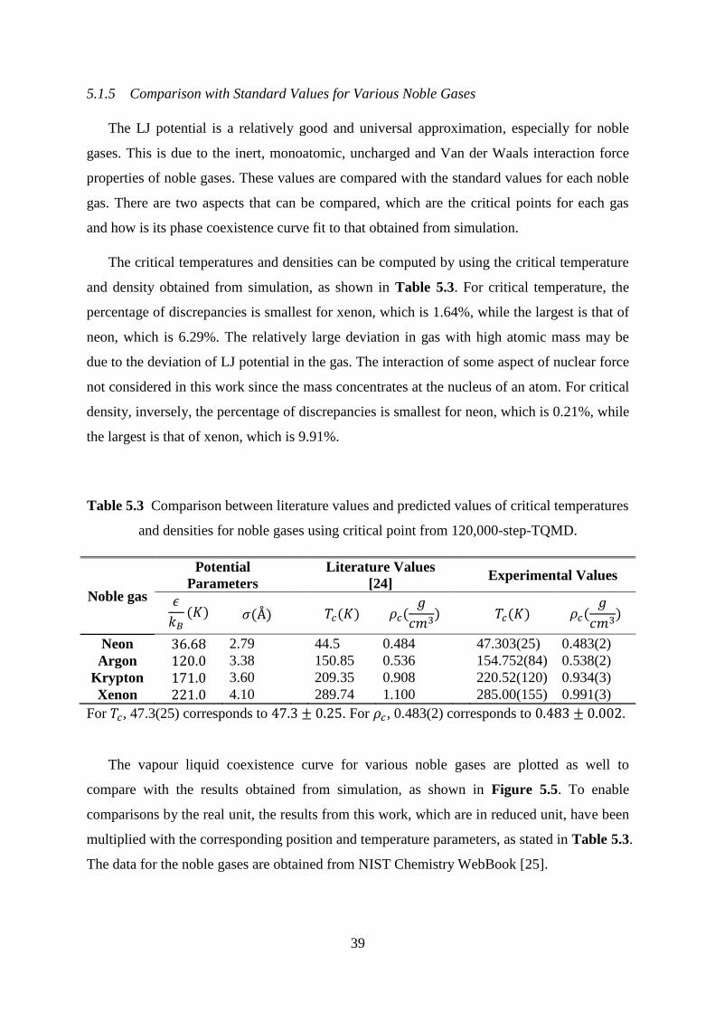
39

5.1.5 Comparison with Standard Values for Various Noble Gases

The LJ potential is a relatively good and universal approximation, especially for noble

gases. This is due to the inert, monoatomic, uncharged and Van der Waals interaction force

properties of noble gases. These values are compared with the standard values for each noble

gas. There are two aspects that can be compared, which are the critical points for each gas

and how is its phase coexistence curve fit to that obtained from simulation.

The critical temperatures and densities can be computed by using the critical temperature

and density obtained from simulation, as shown in Table 5.3. For critical temperature, the

percentage of discrepancies is smallest for xenon, which is 1.64%, while the largest is that of

neon, which is 6.29%. The relatively large deviation in gas with high atomic mass may be

due to the deviation of LJ potential in the gas. The interaction of some aspect of nuclear force

not considered in this work since the mass concentrates at the nucleus of an atom. For critical

density, inversely, the percentage of discrepancies is smallest for neon, which is 0.21%, while

the largest is that of xenon, which is 9.91%.

Table 5.3 Comparison between literature values and predicted values of critical temperatures

and densities for noble gases using critical point from 120,000-step-TQMD.

Noble gas

Potential

Parameters

Literature Values

[24] Experimental Values

( ) ( ) ( ) (

) ( ) (

)

Neon 2.79 44.5 0.484 47.303(25) 0.483(2)

Argon 3.38 150.85 0.536 154.752(84) 0.538(2)

Krypton 3.60 209.35 0.908 220.52(120) 0.934(3)

Xenon 4.10 289.74 1.100 285.00(155) 0.991(3)

For , 47.3(25) corresponds to . For , 0.483(2) corresponds to .

The vapour liquid coexistence curve for various noble gases are plotted as well to

compare with the results obtained from simulation, as shown in Figure 5.5. To enable

comparisons by the real unit, the results from this work, which are in reduced unit, have been

multiplied with the corresponding position and temperature parameters, as stated in Table 5.3.

The data for the noble gases are obtained from NIST Chemistry WebBook [25].

40

Figure 5.5 Comparison between the vapour-liquid coexistence curve from simulation (red)

and that from literature [25] (Blue).

From Figure 5.5, it is found that the agreement between argon and simulation result is the

best among the 4 graphs. However, there are deviations occur in region near the critical point.

It may be due to inaccuracies of the law of rectilinear diameter used to estimate the data in

the region near the critical point. Neon and Krypton both deviate to a certain extent that the

experimental values located at the border of range of error bar. Xenon shows obvious

deviation in the high liquid density region.

The deviations observed from vapour liquid coexistence curves may be caused by error

that occurred in this approximated calculation. LJ potential is a theoretical approach to

approximate the interaction between two uncharged molecules or atoms. However, the real

potential between noble gas atoms is not exactly the LJ potential. It may have some unseen

interactions between the atoms, especially for atoms with high atomic mass like xenon. In

general, this type of potential is used only for simplicity.

41

5.1.6 Comparison by Using Different Methods of Molecular Simulations

There are many types of molecular simulations for LJ fluid. Hence, the results obtained

from the first simulation in this work, which is 120,000-step-TQMD is compared with the

data obtained from Johnson‟s equation of state [26] and grand-canonical transition-matrix

Monte Carlo and histogram re-weighting [27], as shown in Figure 5.6.

From the figure, it shows that the curves are close to each other. There are deviations in

between the curves, especially in the region near the critical point. However, from various

comparisons above, the overall agreement with the results from various literatures is good.

Hence, the TQMD simulation is a method to study the location of phase coexistence of a

system.

Figure 5.6 Comparison by using different methods of molecular simulations: Johnson‟s

equation of state (blue), grand-canonical transition-matrix Monte Carlo and histogram re-

weighting (black) and TQMD (red).

42

5.2 Properties of Lennard-Jones Fluid

Another point of interest in molecular simulation is the variation in some variables and

parameters. To observe how is a variable varies with respect to another; MD simulations are

done by using Mathematica software. Three relations of interest are relations between

temperature and density, pressure and temperature, and, pressure and volume. However, the

number of particles used in these simulations will be less than that of TQMD.

5.2.1 Observations Indicating Phase Transition

To observe the phase of the system throughout the simulation, radial distribution function

(RDF) as a function of interparticle distance, , is plotted at a certain interval. RDF displays

the arrangement of particles in the system, which is giving information about that existing

phase of the system at certain temperature. Figure 5.7 shows the examples of RDF for solid,

liquid and vapor states obtained from simulation.

To indicate the points where phase transition of LJ fluid system occurs, it is expected that

there must be a change in some parameters. Hence, various graphs, which are pressure versus

temperature, potential energy versus temperature and compression factor versus temperature,

are plotted. There is a noticeable change in gradient of these graphs, as shown in Figure 5.8,

which are the examples of the graphs mentioned. This indicates a phase change occurring.

There seems to a discontinuous change in derivative of the graphs when the phase boundary

line is crossed.

5.2.2 Relation Between Temperature and Density

A simulation is set in ensemble. The system consists of 256 atoms and has a cutoff

radius of . The simulation is repeated for various values of density. For densities

that are more or equal than , the system is allowed to run for 20,000 steps with

equilibration after 10,000 steps. Otherwise, for lower densities, the simulation steps are set

differently. For , it runs for 40,000 steps with equilibration after 20,000 steps. For

and , it runs for 30,000 steps with equilibration after 20,000 steps. More

simulation steps are needed for lower density system to account for its increased sensitivity

and more poorly description by LJ potential.

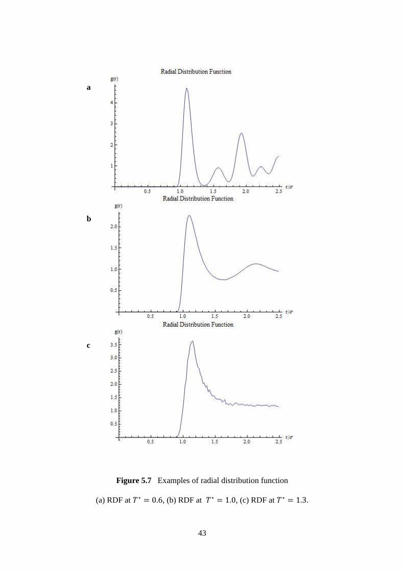
43

Figure 5.7 Examples of radial distribution function

(a) RDF at , (b) RDF at , (c) RDF at .

a

b

c

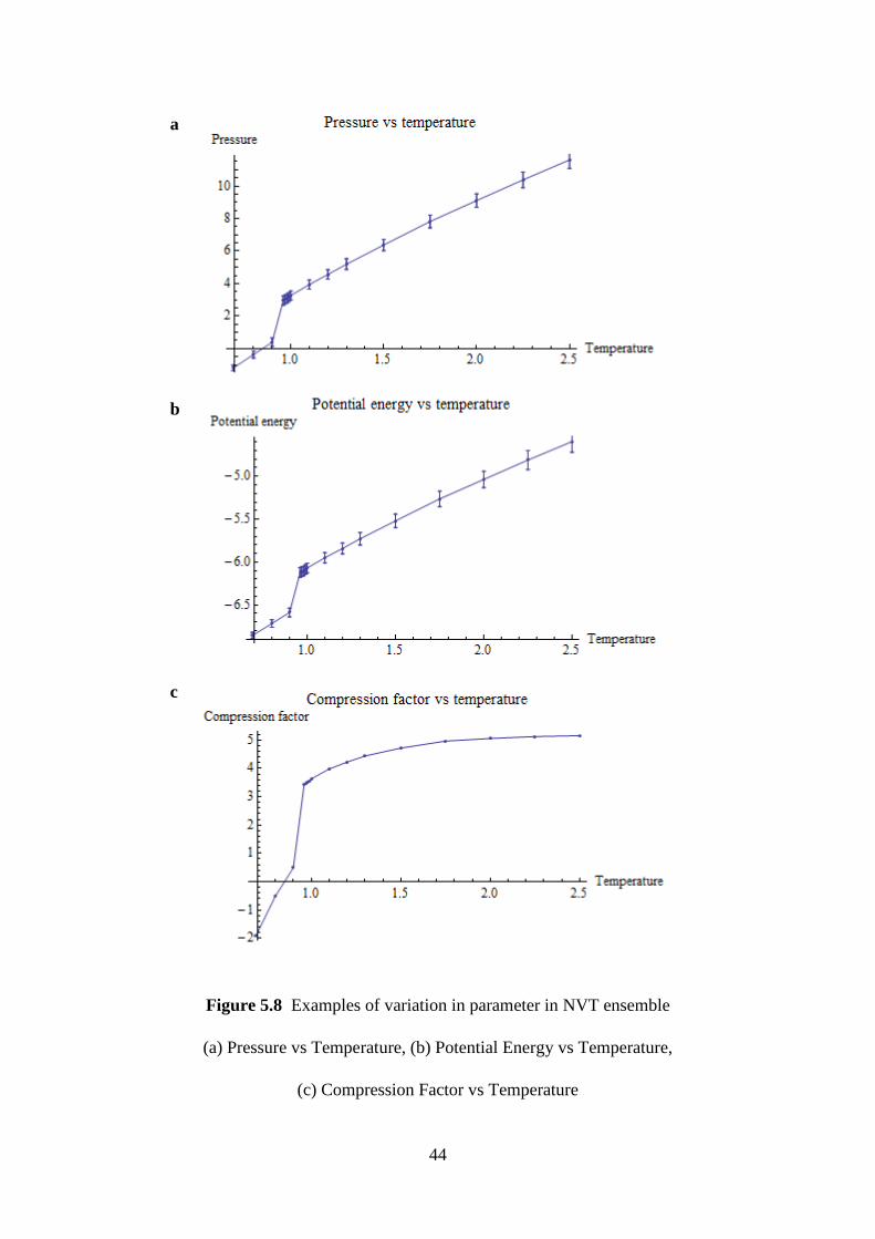
44

Figure 5.8 Examples of variation in parameter in NVT ensemble

(a) Pressure vs Temperature, (b) Potential Energy vs Temperature,

(c) Compression Factor vs Temperature

a

b

c

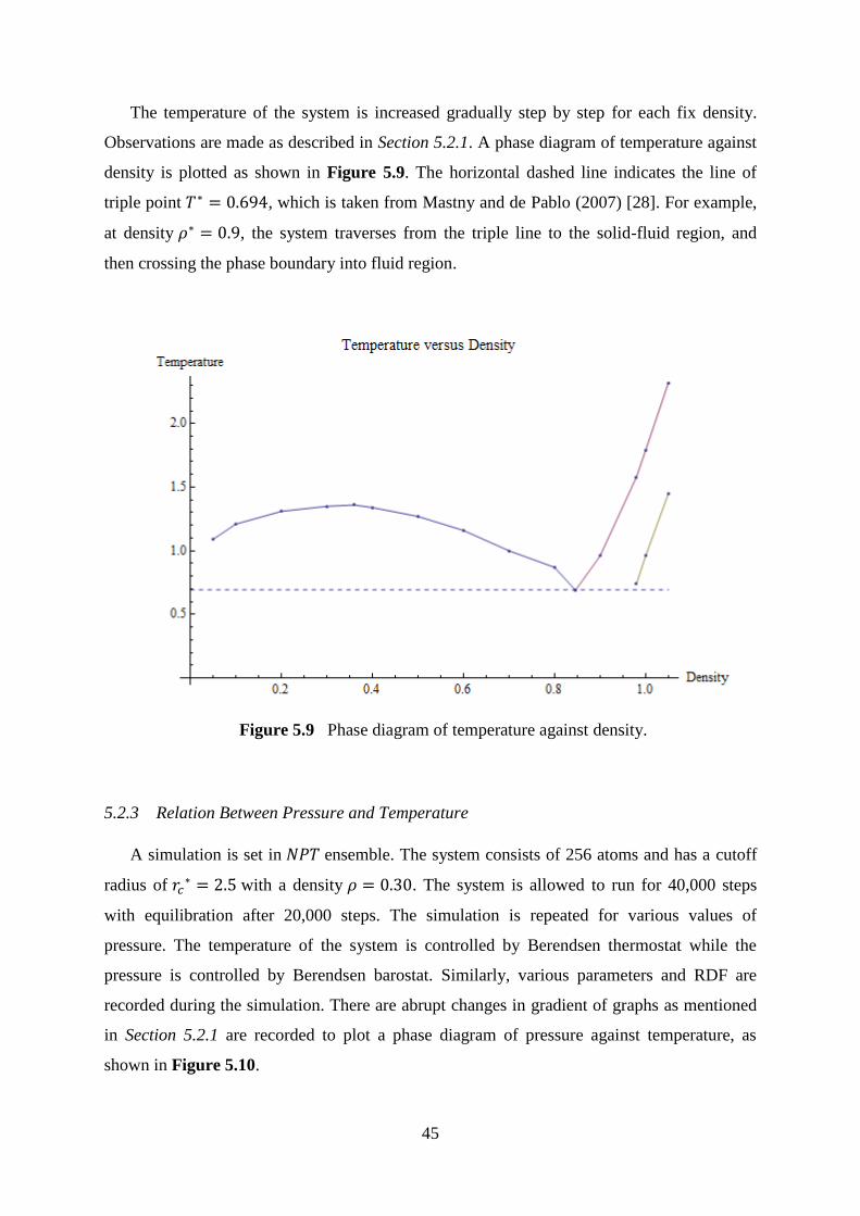
45

The temperature of the system is increased gradually step by step for each fix density.

Observations are made as described in Section 5.2.1. A phase diagram of temperature against

density is plotted as shown in Figure 5.9. The horizontal dashed line indicates the line of

triple point , which is taken from Mastny and de Pablo (2007) [28]. For example,

at density , the system traverses from the triple line to the solid-fluid region, and

then crossing the phase boundary into fluid region.

Figure 5.9 Phase diagram of temperature against density.

5.2.3 Relation Between Pressure and Temperature

A simulation is set in ensemble. The system consists of 256 atoms and has a cutoff

radius of with a density . The system is allowed to run for 40,000 steps

with equilibration after 20,000 steps. The simulation is repeated for various values of

pressure. The temperature of the system is controlled by Berendsen thermostat while the

pressure is controlled by Berendsen barostat. Similarly, various parameters and RDF are

recorded during the simulation. There are abrupt changes in gradient of graphs as mentioned

in Section 5.2.1 are recorded to plot a phase diagram of pressure against temperature, as

shown in Figure 5.10.

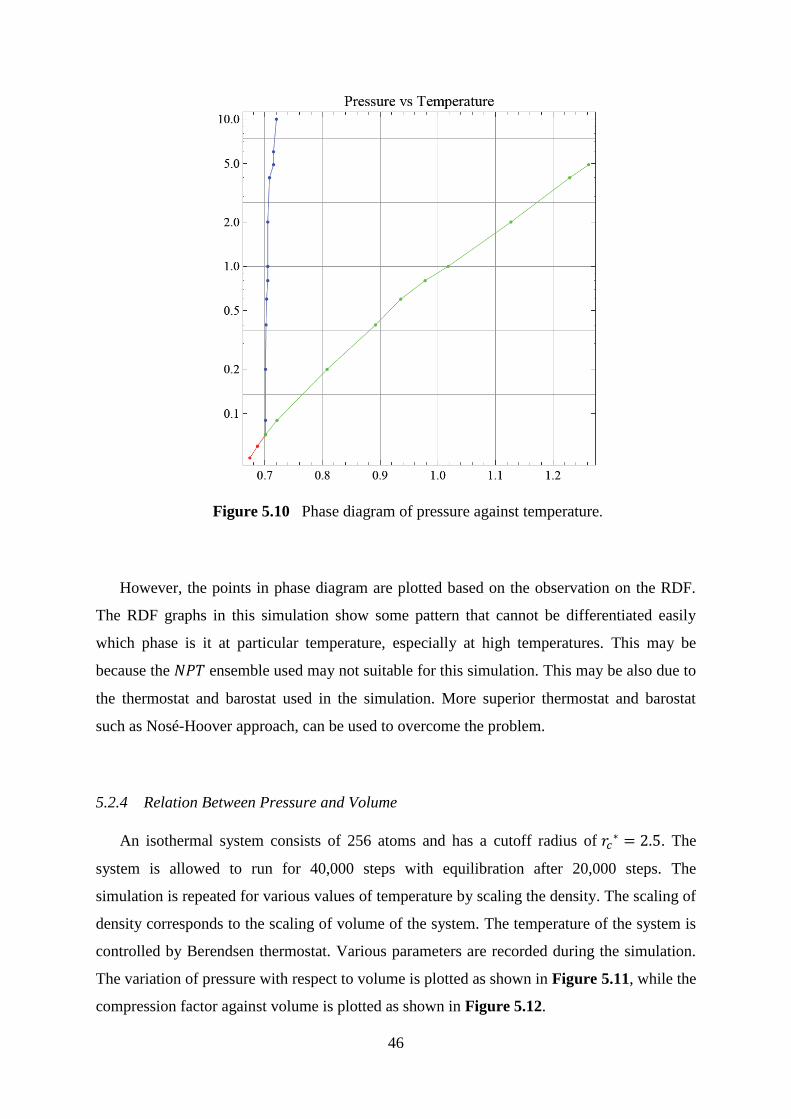
46

Figure 5.10 Phase diagram of pressure against temperature.

However, the points in phase diagram are plotted based on the observation on the RDF.

The RDF graphs in this simulation show some pattern that cannot be differentiated easily

which phase is it at particular temperature, especially at high temperatures. This may be

because the ensemble used may not suitable for this simulation. This may be also due to

the thermostat and barostat used in the simulation. More superior thermostat and barostat

such as Nosé-Hoover approach, can be used to overcome the problem.

5.2.4 Relation Between Pressure and Volume

An isothermal system consists of 256 atoms and has a cutoff radius of . The

system is allowed to run for 40,000 steps with equilibration after 20,000 steps. The

simulation is repeated for various values of temperature by scaling the density. The scaling of

density corresponds to the scaling of volume of the system. The temperature of the system is

controlled by Berendsen thermostat. Various parameters are recorded during the simulation.

The variation of pressure with respect to volume is plotted as shown in Figure 5.11, while the

compression factor against volume is plotted as shown in Figure 5.12.

47

Figure 5.11 Pressure against volume at various temperatures. From the below to top line,

temperature are respectively , , , , , , and .

Figure 5.12 Compression factor against volume at various temperatures. From the

below to top line, temperature are respectively , , , , , ,

and .

48

Figure 5.11 shows the variation of pressure with respect to volume at a constant

temperature. At lowest temperature where , the system behaves like real gas as its

volume increases. At high temperature, it shows that the real gas system behaves like an ideal

gas system. Another interesting point from this figure is the negative pressure of the system

when it has a small volume. This indicates that the interatomic force in this region is

attractive. At high temperature, where the system behaves like ideal gas, this interatomic

force is negligible. The system is expected to behave like an ideal gas at critical temperature

. However, from the graph, the system behaves in such the way only at highest temperature

where .

Figure 5.12 shows the variation of compression factor with respect to volume at a

constant temperature. At high temperature, the compression factor approaches more quickly

to 1.0 than that at low temperature as volume increases. The isotherm at lower temperature

deviates much from the ideal gas law. The top 3 isotherms begin to obey the ideal gas law,

approaching unity quickly as the volume of system is increased. Hence, it clearly shows that

at high temperature, the system behaves like an ideal gas system.

49

CHAPTER 6

CONCLUSION AND RECOMMENDATIONS

6.1 Conclusion

Phase transition and properties of Lennard-Jones (LJ) fluid are investigated by using

molecular dynamics simulation. Temperature-quench molecular dynamics simulation

(TQMD) is employed to study the phase coexistence of LJ fluid and a series of simulations

are carried out in various ensembles by using Mathematica to study its properties.

TQMD locates phase coexistence points based on canonical molecular dynamics

simulation together with a post-simulation analysis method. Two coexisting phases are

separated immediately when temperature is dropped suddenly, which sets the system into a

thermally and mechanically unstable state. Quenches which do not result in phase separation

used to bound coexistence lines and surfaces. TQMD requires only local equilibration in each

sub-cell instead of global equilibration of the system.

The densities and compositions are used in the post-simulation analysis to determine the

critical temperature and density of LJ fluid. The results make good agreement with literature

results and GEMC [1]. The interface, which is avoided using GEMC, can be avoided by the

use of relatively large simulation cells and accessible to modern computing equipment. It

shows that the equilibrium properties can be analyzed when local equilibrium is reached

instead of global equilibrium. Deviations occurred when LJ fluid approximation is applied to

heavy noble gas system, such as xenon.

Phase diagrams are generated by observing the variations of variables and radial

distribution functions plotted by using Mathematica. When there is an abrupt change in each

of these graphs, and typical radial distribution functions display typical pattern for respective

phase, there is a phase change in the system. To study the properties of LJ fluid, the effect of

variation of volume on pressure and compression factor are observed through plotting of

graphs, it shows that the system behaves like an ideal gas when the system has a large volume

at high temperature. This indicates that the system built fulfils the requirement to build a

model of the real system.

50

6.2 Recommendations

To overcome the problem faced in this work, some recommendation steps can be applied

to the work. A better thermostat like Nosé-Hoover thermostat can be employed to control the

temperature of system. Velocity Verlet algorithm can be replaced by a better algorithm like

5th-order Gear predictor–corrector algorithm. Different potential can be used to describe the

interactions between particles according to the need of system.

Future extension to this project can be on the parallelization of TQMD code. Unlike

Monte Carlo methods for molecular simulation, molecular dynamics algorithms may be

efficiently parallelized in many ways. This trend of increasing the availability, lower cost and

simplicity of use of parallel computer setups could be further enhancing the potential of this

method. Binary and multiphase system can also be simulated using temperature-quench

molecular dynamics method due to universality of the method to apply to various systems.

51

REFERENCES

[1] Martínez-Veracoechea*, F., & Müller, E. A. (2005). Temperature-quench Molecular

Dynamics Simulations for Fluid Phase Equilibria. Molecular Simulation, 31, 33-43.

[2] Gelb, L. D., & Müller, E. A. (2002). Location of phase equilibria by temperature-

quench molecular dynamics simulations. Fluid phase equilibria, 203, 1-14.

[3] Giordano, N. J., & Nakanishi, H. (2005). Computational Physics. Addison-Wesley,

United State of America.

[4] van Gunsteren, W. F., & Berendsen, H. J. (1990). Computer simulation of molecular

dynamics: Methodology, applications, and perspectives in chemistry. Angewandte

Chemie International Edition in English, 29(9), 992-1023.

[5] Straatsma, T. P. (2004). Molecular Modeling and Simulation. (Computational Biology

Noontime Seminar Series, Pacific Northwest National Laboratory, July 26, 2004).

[6] Verlet, L. (1967). Computer "experiments" on classical fluids. I. Thermodynamical

properties of Lennard-Jones molecules. Physical review, 159, 98.

[7] Hansen, J. P., & Verlet, L. (1969). Phase transitions of the Lennard-Jones

system. Physical Review, 184, 151.

[8] Nicolas, J. J., Gubbins, K. E., Streett, W. B., & Tildesley, D. J. (1979). Equation of

state for the Lennard-Jones fluid. Molecular Physics, 37, 1429-1454.

[9] Johnson, J. K., Zollweg, J. A., & Gubbins, K. E. (1993). The Lennard-Jones equation

of state revisited. Molecular Physics, 78(3), 591-618.

[10] Panagiotopoulos, A. Z. (1987). Direct determination of phase coexistence properties

of fluids by Monte Carlo simulation in a new ensemble. Molecular Physics, 2002, 100,

237-246.

[11] Panagiotopoulos, A. Z. (1994). Molecular simulation of phase equilibria, Supercritical

Fluids - Fundamentals for Application, E. Kiran. and J. M. H. Levelt Sengers (eds.),

NATO ASI Series E, 273, Kluwer Academic Publishers: Dordrecht, The Netherlands,

pp. 411-437 (1994).

[12] Panagiotopoulos, A. Z. (2000). Monte Carlo methods for phase equilibria of

fluids. Journal of Physics: Condensed Matter, 12(3), R25.

[13] Smit, B. (1996). Molecular simulations of fluid phase equilibria. Fluid phase

equilibria, 116, 249-256.

52

[14] Matsumoto, M. (1998). Molecular dynamics of fluid phase change. Fluid phase

equilibria, 144, 307-314.

[15] Gu K., Watkins, C. B., & Koplik, J. (2010). Molecular dynamics simulation of the

equilibrium liquid–vapor interphase with solidification. Fluid Phase Equilibria,297,

77-89.

[16] Bopp, P. A., Buhn, J. B., Maier, H. A., & Hampe, M. J. (2008). Scope and limits of

molecular simulations. Chemical Engineering Communications,195, 1437-1456.

[17] ChemWiki. University of California, Davis. Lennard-Jones Potential.

“http://chemwiki.ucdavis.edu/Physical_Chemistry/Quantum_Mechanics/Atomic_The

ory/Intermolecular_Forces/Lennard-Jones_Potential”, 23th

April 2013.

[18] Frenkel, D., & Smit, B. (2002). Understanding molecular simulation: from algorithms

to applications. Academic press.

[19] Vlugt, T.J.H., van der Eerden, J.P.J.M., Dijkstra, M., Smit, B., Frenkel, D. (2008).

Introduction to Molecular Simulation and Statistical Thermodynamics. Delft, The

Netherlands.

[20] Material Digital Library Pathway Softmatter: Radial Distribution Function

“http://www.matdl.org/matdlwiki/index.php/softmatter:Radial_Distribution_Function

”, 23th

April 2013.

[21] Buehler, M. J. (2011). Lecture notes, "Property Calculation II", Introduction to

Modeling and Simulation. Department of Civil and Environmental Engineering,

Massachusetts Institute of Technology.

[22] MesoBioNano Explorer. Lennard-Jones Potential.

“http://www.mbnexplorer.com/users-guide/4-energy-and-force-calculation/41-

pairwise-potentials/414-lennard-jones-potential”, 24th

April 2013.

[23] Balasubramanya, M. K., Roth, M. W., Tilton, P. D., & Suchy, B. A. (2006).

Molecular dynamics simulations of noble gas release from endohedral fullerene

clusters. arXiv preprint cond-mat/0607535.

[24] NIST Chemistry WebBook, Thermophysical Properties of Fluid Systems

“http://webbook.nist.gov/chemistry/fluid/”, 25th

April 2013.

[25] Benchmark results for Lennard-Jones fluid, SAT-EOS: Liquid-vapor coexistence

properties

“http://www.cstl.nist.gov/srs/LJ_PURE/sateos.htm”, 24th

April 2013

53

[26] Benchmark results for Lennard-Jones fluid, SAT-TMMC: Liquid-vapor coexistence

properties

“http://www.cstl.nist.gov/srs/LJ_PURE/sattmmc.htm”, 24th

April 2013

[27] Mastny, E. A., & de Pablo, J. J. (2007). Melting line of the Lennard-Jones system,

infinite size, and full potential. The Journal of chemical physics, 127, 104504.

[28] Thijssen, J. (2007). Computational physics. University Press, Cambridge.

[29] Rapaport, D. C. (2004). The art of molecular dynamics simulation. University Press,

Cambridge.

[30] Cameron Abrams (2009). Lecture Notes, CHE 800-002: Molecular Simulation Spring

0304, Drexel University, Philadelphia, March 21 - December 1, 2009.

[31] Swiss Institute of Bioinformatics. Theory of Molecular Dynamics Simulations.

“http://www.ch.embnet.org/MD_tutorial/pages/MD.Part1.html”, 26th

April 2013.

[32] Victor Rühle (2007). Berendsen and Nose-Hoover thermostats. Private paper.

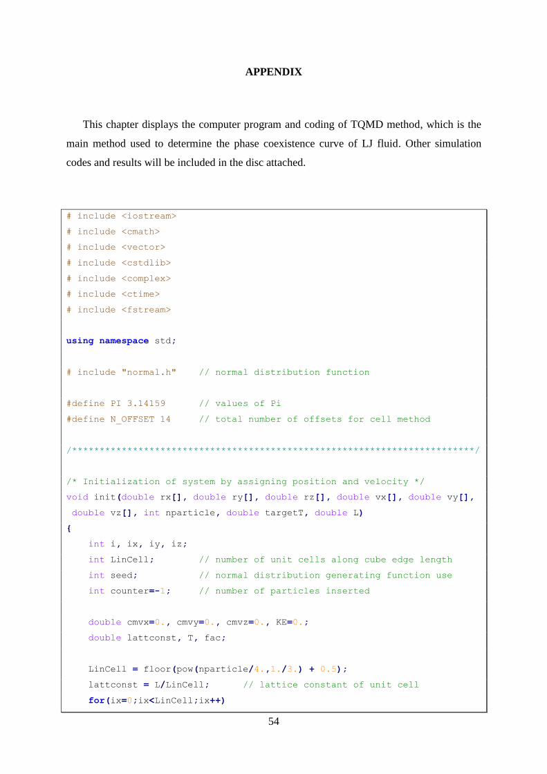
54

APPENDIX

This chapter displays the computer program and coding of TQMD method, which is the

main method used to determine the phase coexistence curve of LJ fluid. Other simulation

codes and results will be included in the disc attached.

# include <iostream>

# include <cmath>

# include <vector>

# include <cstdlib>

# include <complex>

# include <ctime>

# include <fstream>

using namespace std;

# include "normal.h" // normal distribution function

#define PI 3.14159 // values of Pi

#define N_OFFSET 14 // total number of offsets for cell method

/*************************************************************************/

/* Initialization of system by assigning position and velocity */

void init(double rx[], double ry[], double rz[], double vx[], double vy[],

double vz[], int nparticle, double targetT, double L)

{

int i, ix, iy, iz;

int LinCell; // number of unit cells along cube edge length

int seed; // normal distribution generating function use

int counter=-1; // number of particles inserted

double cmvx=0., cmvy=0., cmvz=0., KE=0.;

double lattconst, T, fac;

LinCell = floor(pow(nparticle/4.,1./3.) + 0.5);

lattconst = L/LinCell; // lattice constant of unit cell

for(ix=0;ix<LinCell;ix++)

55

{

for(iy=0;iy<LinCell;iy++)

{

// assignning particle to a unit cell in fcc lattice

for(iz=0;iz<LinCell;iz++)

{ // 4 particles in a unit cell

counter++;

rx[counter]=(ix+0.25)*lattconst;

ry[counter]=(iy+0.25)*lattconst;

rz[counter]=(iz+0.25)*lattconst;

counter++;

rx[counter]=(ix+0.75)*lattconst;

ry[counter]=(iy+0.75)*lattconst;

rz[counter]=(iz+0.25)*lattconst;

counter++;

rx[counter]=(ix+0.75)*lattconst;

ry[counter]=(iy+0.25)*lattconst;

rz[counter]=(iz+0.75)*lattconst;

counter++;

rx[counter]=(ix+0.25)*lattconst;

ry[counter]=(iy+0.75)*lattconst;

rz[counter]=(iz+0.75)*lattconst;

}

}

}

seed = time(NULL); // initialization for normal.h

for(i=0;i<nparticle;i++) // assignning velocity to particles

{

vx[i] = r8_normal_01 ( seed );

vy[i] = r8_normal_01 ( seed );

vz[i] = r8_normal_01 ( seed );

}

for(i=0;i<nparticle;i++) // total velocity along a dimension

{

cmvx += vx[i];

cmvy += vy[i];

56

cmvz += vz[i];

}

for(i=0;i<nparticle;i++) // remove velocity of center of system

{

vx[i] -= cmvx/nparticle;

vy[i] -= cmvy/nparticle;

vz[i] -= cmvz/nparticle;

KE += vx[i]*vx[i]+vy[i]*vy[i]+vz[i]*vz[i];

}

KE*=0.5; // kinetic energy

T=KE/nparticle*2./3.; // temperature

fac=sqrt(targetT/T); // temperature rescaling factor

KE=0;

for(i=0;i<nparticle;i++) // velocity rescaling

{

vx[i] *= fac;

vy[i] *= fac;

vz[i] *= fac;

KE += vx[i]*vx[i]+vy[i]*vy[i]+vz[i]*vz[i];

}

KE*=0.5; // new kinetic energy

}

/***********************************************************************/

// function to wrap the cell due to periodic boundary

void cellwrap(int &var, double &change, int cells, double L)

{

if(var >= cells){ // when variable exceeds max number of cells

var = 0;

change = L; // position wrap

}

else if(var < 0){ // when variable does not belong to any cell

var = cells - 1;

change = -L; // position wrap

}

}

57

/*************************************************************************/

/*

Cell subdivison method is used to reduces the computational effort to the

O(N) level. Simulation region is divided into a lattice of small cells, and

that the cell edges all exceed rc in length. Atoms are assigned to cells on

the basis of their current positions, so that interactions are only

possible between atoms that are either in the same cell or in immediately

adjacent cells. Due to symmetry only half the neighboring cells need be

considered

A linked list is used to store the required data about cell no. and

position of particles. Each linked list requires a separate pointer f to

access the first data item, and the item terminating the list must have a

special pointer value, 1 in our case. f = a points to a-th particle as the

first item in the list, p_a = b points to b-th particle as the second item,

and so on, until a pointer value p_z = 1 is encountered, terminating the

list. In summary, linked lists are used to associate atoms with the cells

in which they reside at any given instant.

Normally each a separate list is required for each cell. However rather

than use separate arrays for the two kinds of pointer, namely that between

atoms in the same cell and that to the first particle in a cell, the first

nparticle elements in array cellList are used for the former and the

remainer for the latter. This method is introduced in The Art of Molecular

Dynamics Simulation by D. C. Rapaport.

*/

// computation of forces

double compute(double rx[], double ry[], double rz[], double fx[],

double fy[], double fz[], int *gr, int nparticle, double L, double rc,

int n, int nEqui, int grs, double &vir, double ecut, double ecor,

double dh, int cells, int cellList[])

{

// declaration of function

void cellwrap(int &, double &, int, double);

58

// common variable declaration

int i,j1,j2,bin; // for loop variables and bin counting

double dx,dy,dz; // distance between a pair of particles

double e=0., hL=L/2.0; // potential energy and half cube edge length

double f, r2, rc2, r6i; // variable for force calculation

// cell list variable declaration

double shiftx, shifty, shiftz; // shift of cell due to PBC

int ccx, ccy, ccz, c, m1x, m1y, m1z, offset;

int m1, m2vx, m2vy, m2vz, m2;

int vOff[14][3]={{0,0,0}, {1,0,0}, {1,1,0}, {0,1,0},{-1,1,0},{0,0,1}, \

{1,0,1}, {1,1,1}, {0,1,1}, {-1,1,1}, {-1,0,1}, \

{-1,-1,1}, {0,-1,1}, {1,-1,1}}; // offsets of the 14 neighbor cells

// Initialization

rc2=rc*rc;

for(i=0;i<nparticle;i++) // set initial force to zero

{

fx[i]=fy[i]=fz[i]=0.;

}

vir=0.; // set virial value to zero

// Cell list method initialization

for(i=nparticle;i<(nparticle+cells*cells*cells);i++) cellList[i] = -1;

for(i=0;i<nparticle;i++) // assigning each particle to cell

{

ccx = rx[i]/(L/cells); // cell no. along a given dimension

ccy = ry[i]/(L/cells);

ccz = rz[i]/(L/cells);

// cell no. in scalar form

c = ((ccz * cells + ccy) * cells + ccx) + nparticle;

cellList[i] = cellList[c]; // form a linked list for the cells

cellList[c] = i;

}

for (m1z = 0; m1z < cells; m1z++) // looping of cells

{

for (m1y = 0; m1y < cells; m1y ++)

{

for (m1x = 0; m1x < cells; m1x ++)

{

59

// cell no.

m1 = ((m1z * cells + m1y) * cells + m1x) + nparticle;

// looping of neighbor cells

for (offset = 0; offset < N_OFFSET; offset ++)

{

// numbers of the neighboring cell

m2vx = m1x + vOff[offset][0];

m2vy = m1y + vOff[offset][1];

m2vz = m1z + vOff[offset][2];

shiftx=shifty=shiftz=0.;

// periodic boundary of cell

cellwrap(m2vx, shiftx, cells, L);

cellwrap(m2vy, shifty, cells, L);

cellwrap(m2vz, shiftz, cells, L);

// scalar cell no. of the neighboring cell.

m2 = ((m2vz * cells + m2vy) * cells + m2vx) +

nparticle;

// non-sequential progression of cell elements

for (j1 = cellList[m1]; j1 >= 0; j1 = cellList[j1])

{

for (j2 = cellList[m2]; j2 >= 0; j2 = cellList[j2])

{

// avoid double counting

if (m1 != m2 || j2 < j1)

{

// pair distance

dx = rx[j1] - rx[j2];

dy = ry[j1] - ry[j2];

dz = rz[j1] - rz[j2];

// change of distance due to PBC

dx -= shiftx;

dy -= shifty;

dz -= shiftz;

// sum of squares

r2 = dx*dx + dy*dy + dz*dz;

// enter if located within cut-off radius

if(r2<rc2)

{

r6i = 1./(r2*r2*r2);

// potential energy calculation

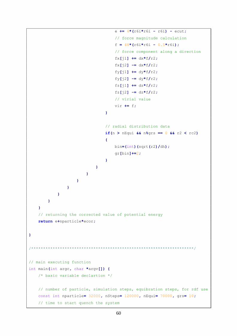
60

e += 4*(r6i*r6i - r6i) - ecut;

// force magnitude calculation

f = 48*(r6i*r6i - 0.5*r6i);

// force component along a direction

fx[j1] += dx*f/r2;

fx[j2] -= dx*f/r2;

fy[j1] += dy*f/r2;

fy[j2] -= dy*f/r2;

fz[j1] += dz*f/r2;

fz[j2] -= dz*f/r2;

// virial value

vir += f;

}

// radial distribution data

if(n > nEqui && n%grs == 0 && r2 < rc2)

{

bin=(int)(sqrt(r2)/dh);

gr[bin]+=2;

}

}

}

}

}

}

}

}

// returning the corrected value of potential energy

return e+nparticle*ecor;

}

/********************************************************************/

// main executing function

int main(int argc, char *argv[]) {

/* basic variable declartion */

// number of particle, simulation steps, equibration steps, for rdf use

const int nparticle= 32000, nSteps= 120000, nEqui= 70000, grs= 10;

// time to start quench the system

61

int ndrop= 20000;

int ngr, nHis, i, n; // variable for RDF use

int * gr;

double * doublegr;

clock_t t1,t2; // for execution time calculation

// density, time steps, cut-off radius, berendsen coefficient

double rho = 0.328, dt = 0.004, rc = 5.0, tau = 0.1;

// initial temperature, quench temperature, temperature variable

double initT = 4.0, finalT = 0.7, targetT;

// general needed variable like correction terms of potential energy

double V, L, rr3, ecor, pcor, ecut, dt2, rc2, dh;

double T, stemp, temp, P, spres, pres, sPE, vPE;

double vb, nid;

// potential and kinetic energy, virial, thermostat ratio

double PE, KE, vir, lambda;

// forces of particle

double fx[nparticle], fy[nparticle], fz[nparticle];

// positions of particle

double rx[nparticle], ry[nparticle], rz[nparticle];

// velocities of particle

double vx[nparticle], vy[nparticle], vz[nparticle];

// for calculating execution time

t1=clock();

V = nparticle/rho; // volume of system

L = pow(V,1./3.); // cube edge length

rc= min(rc,L/2); // minimum between cut0off radius and half length

rr3 = 1/pow(rc,3.);

// potential energy correction term

ecor = 8*PI*rho*(rr3*rr3*rr3/9.0 - rr3/3.0);

// pressure correction term

pcor = 16.0/3.0*PI*rho*rho*(2./3.*rr3*rr3*rr3 - rr3);

// shifted potential energy calue

ecut = 4.*(pow(rr3,4.) - pow(rr3,2.));

rc2 = pow(rc,2.);

dt2 = pow(dt,2.);

/* cell list variable declaration */

62

// number of cell along a dimension

int cells = L/rc;

// array storing cell information

int cellList[cells*cells*cells + nparticle];

// set the initial temperature

targetT = initT;

// initialize the sum of temperature, pressure and potential energy

stemp=0.0;

spres=0.0;

sPE=0.0;

/* variable used to calculate radial distribution function (rdf) */

ngr = 0;

dh = 0.02;

nHis = (int)(rc/dh);

gr = (int*)calloc(nHis,sizeof(int));

doublegr = (double*)calloc(nHis,sizeof(double));

/* intialization of system */

// calling functions

init(rx,ry,rz,vx,vy,vz,nparticle,targetT,L);

PE = compute(rx, ry, rz, fx, fy, fz, gr, nparticle, L, rc, 1,

nEqui, grs, vir, ecut, ecor, dh, cells, cellList);

cout << "Number of particles: " << nparticle << endl;

/****************** starting the simulation ******************/

for(n=0;n<nSteps;n++) // looping of simulation steps

{

if(n%1000==0) cout << n << endl;

// quenching of system is done

if(n==ndrop) targetT = finalT;

/* First integration half-step */

for(i=0;i<nparticle;i++)

{

// first part of velovity Verlet algorithm

rx[i]+=vx[i]*dt+0.5*dt2*fx[i];

63

ry[i]+=vy[i]*dt+0.5*dt2*fy[i];

rz[i]+=vz[i]*dt+0.5*dt2*fz[i];

vx[i]+=0.5*dt*fx[i];

vy[i]+=0.5*dt*fy[i];

vz[i]+=0.5*dt*fz[i];

/* Apply periodic boundary conditions */

if (rx[i]<0.0) rx[i]+=L; else if (rx[i]>L) rx[i]-=L;

if (ry[i]<0.0) ry[i]+=L; else if (ry[i]>L) ry[i]-=L;

if (rz[i]<0.0) rz[i]+=L; else if (rz[i]>L) rz[i]-=L;

}

// Calculate forces

PE = compute(rx, ry, rz, fx, fy, fz, gr, nparticle, L, rc,

n, nEqui, grs, vir, ecut, ecor, dh, cells, cellList);

// required for normalization of radial distribution function

if(n > nEqui && n%grs == 0) ngr++;

/* Second part of velocity Verlet algorithm */

KE = 0.0;

for(i=0;i<nparticle;i++)

{

vx[i]+=0.5*dt*fx[i];

vy[i]+=0.5*dt*fy[i];

vz[i]+=0.5*dt*fz[i];

KE+=vx[i]*vx[i]+vy[i]*vy[i]+vz[i]*vz[i];

}

KE*=0.5;

/* Berendsen thermostat */

// Berendsen coefficient

lambda = sqrt(1 + dt/tau*(targetT/(2.0*KE/3.0/nparticle) - 1.0));

KE=0.0;

for(i=0;i<nparticle;i++) // rescaling velocity

{

vx[i]*=lambda;

vy[i]*=lambda;

vz[i]*=lambda;

KE+=vx[i]*vx[i]+vy[i]*vy[i]+vz[i]*vz[i];

}

KE*=0.5;

64

/* determine the current state propeties */

temp = KE/nparticle*2./3.;

if(n>nEqui) stemp+=temp;

pres = rho*KE*2./3./nparticle + vir/3.0/V + pcor;

if(n>nEqui) spres+=pres;

if(n>nEqui) sPE+=PE;

}

/* normalizing radial distribution function */

for(i=0;i<nHis;i++)

{

vb = ((i+1)*(i+1)*(i+1)-i*i*i)*dh*dh*dh;

nid = (4./3.)*PI*vb*rho;

doublegr[i]=(double)(gr[i])/(ngr*nparticle*nid);

}

/**************************** output ******************************/

/* radial distribution function data */

ofstream file1 ("rdf.txt");

for(i=0;i<nHis;i++)

{

file1 << "{" << dh*(i+0.5) << "," << doublegr[i] << "}" << endl;

}

file1.close();

/* state variables */

T = stemp/(nSteps-nEqui);

P = spres/(nSteps-nEqui);

vPE = sPE/nparticle/(nSteps-nEqui)+ecor;

ofstream file2 ("variable.txt");

file2 << "The temperature is " << T << endl;

file2 << "The pressure is " << P << endl;

file2 << "The potential energy is " << vPE << endl;

file2.close();

cout << "The temperature is " << T << endl;

65

cout << "The pressure is " << P << endl;

cout << "The potential energy is " << vPE << endl << endl;

/* position of particles at final configuration */

ofstream file3 ("position.txt");

for(i=0;i<nparticle;i++)

{

file3 << "{" << rx[i] << "," << ry[i] << "," << rz[i]

<< "}" << endl;

}

file3.close();

// calculating execution time

t2=clock();

cout << (t2-t1)/CLOCKS_PER_SEC;

cin.get();

return 0;

}