Purchasing power parity and the theory of general ... · PDF filePurchasing power parity and the theory of general relativity: the ﬁrst tests Jerry Coakleya, ... (PPP), deﬁned

Journal of International Money and Finance

24 (2005) 293–316

www.elsevier.com/locate/econbase

Purchasing power parity and thetheory of general relativity: the first tests

Jerry Coakleya, Robert P. Floodb, Ana M. Fuertesc,Mark P. Taylord,*

aUniversity of Essex, UKbInternational Monetary Fund and National Bureau for Economic Research, USA

cCass Business School, City University, London, UKdUniversity of Warwick and Centre for Economic Policy Research, UK

Abstract

We implement novel tests of general relative purchasing power parity (PPP), defined asa long-run unit elasticity of the nominal exchange rate with respect to relative national prices,

allowing for potentially permanent real exchange rate shocks. The finite-sample properties ofthe estimators used are analyzed through Monte Carlo analysis, allowing for countryheterogeneity, cross-sectional dependence and non-stationary disturbances. Application to

panel data sets of industrialized and developing economies reveals that inflation differentialsare on average reflected one-for-one in long-run nominal exchange rate depreciationdi.e. thatgeneral relative PPP holds.

� 2004 Published by Elsevier Ltd.

JEL classification: C32; F31

Keywords: Real exchange rate; Purchasing power parity; Cross-sectional dependence; Monte Carlo

* Corresponding author. Department of Economics, University of Warwick, Coventry CV4 7AL, UK.

Tel.: C44 24 765 72832; fax: C44 24 765 73013.

E-mail address: [email protected] (M.P. Taylor).

0261-5606/$ - see front matter � 2004 Published by Elsevier Ltd.

doi:10.1016/j.jimonfin.2004.12.008

mailto:[email protected]

http://www.elsevier.com/locate/econbase

294 J. Coakley et al. / Journal of International Money and Finance 24 (2005) 293–316

1. Introduction

Purchasing power parity (PPP) involves a relationship between a country’sforeign exchange rate and the level or movement of its national price level relative tothat of a foreign country. Absolute PPP states that the purchasing power of a unit ofdomestic currency is exactly the same in the foreign economy, once it is convertedinto foreign currency at the absolute PPP exchange rate. Relative PPP implies thatchanges in national price levels are offset by commensurate changes in the nominalexchange rates between the relevant currencies. The voluminous research literatureon PPP published in recent decades has been driven by econometric problemsrelating to univariate and panel unit root tests of necessary conditions for long-runabsolute PPP to hold, in particular whether the real exchange rate has any tendencyto settle down to a long-run equilibrium level.1 These include issues such as lowpower, possible structural breaks, the mixture of stationary and non-stationary errorterms in the relevant regressions, and neglected cross-sectional dependence when realexchange rate panel data are used.

In this paper, we generalize the concept of long-run relative PPP to the case wherethe long-run elasticity of the nominal exchange rate with respect to relative nationalprices is unity without restricting the innovation sequence to be stationary. This iswhat we term general relative PPP. We then develop methods to test for generalrelative PPP in a panel regression framework that is robust to country heterogeneityand cross-sectional dependence as well asdmost importantlydpermanent andtransitory shocks to the real exchange rate. Thus, we allow for the long-runequilibrium real exchange rate to shift while still testing for a long-run unit elasticityof the nominal exchange rate with respect to the price relative.

In contrast, the extant empirical analysis of PPP generally precludes permanentshocks to the long-run real exchange rate. It is widely accepted, however, that over longperiods, real shocks may permanently impact on the long-run equilibrium realexchange rate level due to productivity differentials as in the Harrod-Balassa-Samuelson effect (Froot and Rogoff, 1995; Sarno and Taylor, 2002; Lothian andTaylor, 2004; Bergin et al., 2003). By exploiting recent developments in theeconometrics of non-stationary panel data, we can accommodate such shocksalongside transitory or monetary shocks. Moreover, Taylor (2001) has demonstratedhow two problemsdtrading costs and risk aversion on the one hand and temporalaggregation on the otherdcan make the regression errors of nominal exchange rateson price relatives appear rather persistent or even non-stationary. In developing ourtest procedures, we extend the relevant econometric literature to allow for cross-sectional dependence andmixed stationary and non-stationary errors and compare thefinite-sample properties of several panel estimators using Monte Carlo simulations.

Our empirical analysis is based on a unique, large data set for the 1970:1–1998:12period that comprises 19 Organizations for Economic Cooperation and Development(OECD) member countries and 26 developing countries and both consumer price

1 See Taylor (1995), Sarno and Taylor (2002) and Taylor and Taylor (2004) for overviews.

295J. Coakley et al. / Journal of International Money and Finance 24 (2005) 293–316

index (CPI) and producer price index (PPI) data. Analyzing developing and industrialcountry panels using the same methodology is interesting. The former show largerheterogeneity, more cross-sectional variation (higher signal) but more time seriesnoise also due to measurement error. Our empirical work suggests strongly thatgeneral relative PPP held in each of the panels examined over the data period inquestion, thereby confirming the earlier analysis of Flood and Taylor (1996), whichwas based on informal scatter plots and regression analysis of long-period averages.

The remainder of the paper is organized as follows. In Section 2 we discuss furtherthe notion of general relative PPP. In Section 3 we present the panel econometricframework and explore the finite-sample properties of the estimators employed. Ourempirical results are discussed in Section 4 and we conclude in a final section.

2. General relative PPP

Denote the price level of the domestic currency by Pt and the correspondingforeign price level by Pt

*. If St is the nominal exchange rate (domestic price of foreigncurrency) and if absolute PPP holds, then expressing the domestic price in foreigncurrency terms must yield the foreign price, Pt

*Z Pt/St. Taking logarithms (lowercase) and rearranging, we have the short-term relationship:

stZpt � p)t ð1Þ

which implies that the nominal exchange rate should be directly proportional to therelative price level even in the very short run. The short-run relative PPP conditionmay be written:

DstZDpt �Dp)t or dstZdpt � dp)t ð2Þ

where D and d denote the first difference and total differential operators, respectively.While empirical tests of these short-term relationships were not uncommon in theearly 1970s (see, e.g., Frenkel, 1976; or the studies cited in Officer, 1982), the veryhigh volatility of nominal exchange rates compared to relative national price levelsor inflation rates during the recent floating period has adequately demonstrated thatneither absolute nor relative PPP is a realistic description of short-run exchange ratebehavior.

Instead, over the past few decades, PPP has been extensively tested as a long-runequilibrium condition, largely through unit-root and cointegration methods.Effectively, what unit-root studies do is firstly to capture the short-run variation inreal exchange rates by adding an error term:

stZ�pt � p)t

�Cut ð3Þ

and then to test the hypothesis that the process utdthe deviation from PPPdis non-stationary.2 In particular, if ut contains a random walk or unit-root componentdut

2 The cointegration variant of this is to estimate slope coefficient in this relationship rather than

imposing that they be (1,�1) and then test for a unit root in ut (Taylor, 1988).


is I(1)dthen the implication is that deviations from PPP never settle down at anequilibrium level even in the long run.3 This approach has spawned a vast literaturewhich has, in general, found remarkable difficulty in supporting the hypothesis oflong-run PPP using data for the recent floating rate period alone (Sarno and Taylor,2002; Taylor and Taylor, 2004). Moreover, it has indicated that real exchange ratesor deviations from long-run PPP are extremely persistent, a stylized fact whichRogoff (1996) has described as ‘the PPP puzzle’.

While it is clear that unit root analysis involves a test of long-run PPP, the unitroot approach is rather restrictive since it implies that the level of the exchange rateis not subject to permanent shocks. The concept of general relative PPP that weare proposing here operationalizes, in the context of PPP tests, the ceteris paribusassumption of traditional economic analysis. Suppose that ut in Eq. (3) isobservationally I(1), perhaps due to Harrod-Balassa-Samuelson effects or otherreal shocks. Now further assume that the equation still holds in the sense that thecoefficient on the relative price termdthe elasticity of the nominal exchange ratewith respect to relative pricesdis in fact unity, as in Eq. (3). This can be interpretedas a form of long-run relative PPP in the sense that a 1% increase in relative priceswould still be offset one-to-one by a long-run depreciation of 1%, ceteris paribus,even though long-run PPP would be rejected in the conventional unit-rootframework and both absolute and relative PPP would also be rejected.

The ceteris paribus clause here is crucial. The concept we are proposing is verygeneral. It would allow, for example, for real shocks permanently to affect the realexchange rate so long as any given percentage movement in relative prices wouldlead to a commensurate movement in the nominal exchange rate in the long run,over and above any such permanent effect on the real exchange rate. It is because ofthe generality of the concept that we term it general relative PPP. Note that generalrelative PPP does not imply any particular causality. Although we are testing fora unit elasticity of the exchange rate with respect to relative prices, the concept makesno assertions concerning which way or ways causality runs between the variablesconcerned. It only asserts that, ceteris paribus, in the long run a given percentagechange in relative prices will be offset by a commensurate percentage change in thenominal exchange rate.

Another way of highlighting the distinctive nature of our approach is explicitly tointroduce the long-run, equilibrium real exchange rate, qt in Eq. (3)4:

stZqtC�pt � p)t

�Cvt ð4Þ

where vt is a stationary, zero-mean process. Thus the real exchange rate can bewritten as:

qtZqtCvt: ð5Þ

3 A series is said to be ‘integrated of order d’, I(d ), if it must be differenced d times to become stationary.4 We are grateful to an anonymous referee for this helpful suggestion.


The critical distinction between traditional tests of long-run absolute and relativePPP and our methodology is that the former two assume that qt fluctuates randomlyaround a constant qtZq. If absolute PPP holds then qZ0 but relative PPP impliesqZc where cs 0. No such restrictions apply in our test of long-run general relativePPP. Instead, qt can be time-varying and behave like an I(1) process due to Balassa-Samuelson or other real effects.

Thus, a test of general relative PPP is an economically meaningful test irrespectiveof the behavior of uit in the following log level panel regression

sitZaiCbi

�pit � p)it

�Cuit; tZ1;.;T ð6Þ

where, since qit is unobserved, one can assume that uitZqitCvit for iZ1;.;Ncountries. The object is to estimate the mean of the slope bi that can be interpreted asthe long-run relative price elasticity of the nominal exchange rate for country i. Theinnovation sequence can be I(0) or I(1). The null hypothesis that general relative PPPholds is

H0 : bhEðbiÞZ1 ð7Þ

and the alternative is that bs 1. The expression for the slope, bih dsit/d( pit� pit))

can be obtained either by differentiating Eq. (6) with respect to the price differentialor by rearranging the total differential in Eq. (2) as in the textbook exposition ofrelative PPP. Thus our null of a unit relative price elasticity is consistent with relativePPP but is more general due to the lack of restrictions on uit.

We introduce below a robust panel framework to test for general relative PPP.Our approach can accommodate a number of factors germane to the PPP debate.One is the observed high persistence of real exchange rates that may reflecta combination of real and monetary (or permanent and transitory) shocks. It mayalso relate to the noise stemming from measurement error, transaction costs andother market imperfections such as limits to arbitrage in foreign exchange markets(Taylor and Taylor, 2004) that can make the regression disturbances observationallyequivalent to I(1) series. Another important factor is cross-sectional dependencewhich has typically been neglected in much empirical analysis.

3. Econometric framework

3.1. Non-stationary panel regression

Suppose the data are generated according to the set of relationships

yitZaiCbixitCvit; iZ1;.;N; tZ1;.;T ð8Þ


where aiZ aC ha,i and biZ bC hb,i. This random coefficients model (RCM)assumes that:

(A.1) The coefficients are constant over time but may differ randomly across units,that is, ha,iw iid(0,sa

2), hb,iw iid(0,sb2) and (ha,i,hb,i)# are distributed in-

dependently of the regressor xit and disturbances vit for all i and t.(A.2) The disturbances have a zero mean, time constant but possibly heterogeneous

variance and are uncorrelated across different units, i.e. E(vit)Z 0, E(vit2)Z

si2 and E(vitvjt)Z 0 if is j.

(A.3) The xit and vis are independently distributed for all t, s (strict exogeneity).

The goal is to measure the mean effect bh E(bi) where bi represents the long-runrelation between two I(1) variables. For single time series (NZ 1), analogously to theslope coefficient in the classical linear regression model, a long-run associationbetween yt and xt is defined as bZ

Pyx

Pxx�1 where

Pyx and

Pxx are the long-run

covariance and long-run variance, respectively. When the long-run variance–covariance matrix

Pis rank deficient, b is a cointegrating coefficient. When yt and

xt do not cointegrate (full rankP), b still represents a statistical long-run relationship

as shown by Phillips and Moon (1999). How to estimate b is a different issue.The OLS regression of yt onto xt when

Phas full rank will be spurious (Granger

and Newbold, 1974). However, suppose that independent observations ( yit xit)# areavailable on a large number of countries iZ 1,.,N. Different panel procedures canbe used to estimate b consistently. First, the within or fixed effects (FE) estimatorimposes homogeneous slopes and error variances but allows for heterogenousintercepts. Second, the Pesaran and Smith (1995) mean group (MG) estimatoraverages over the individual OLS regression coefficients bi.

5 This estimator allowsfor heterogeneous intercepts, slopes and error variances. Third, the between or cross-section (CS) estimator involves running an OLS regression for individual means yiand xi. Pesaran and Smith (1995) note that the spurious correlation problem doesnot arise in the case of the CS estimator under the RCM assumptions. Phillips andMoon (1999) further show that both bFE and bCS are

ffiffiffiffiN

p� consistent for b when the

error term vit in Eq. (8) is I(1).Coakley et al. (2001) use Monte Carlo simulations and response surface

regressions to evaluate the finite-sample properties of the FE and MG estimatorfor panel dimensions N, TZ {(15, 300), (30, 25)} typical of monthly and annual PPPstudies, respectively. They show for a non-stationary regression such as Eq. (8) thatboth estimators appear unbiased with dispersion that falls at rate T

ffiffiffiffiN

pwhen vit is

I(0) and at rateffiffiffiffiN

pwhen vit is I(1).

6 Moreover, standard t-tests based on the N(0, 1)quantiles have good size properties in the MG case irrespective of whether theregression disturbances are I(0) or I(1). By contrast, inference based on the FE

5 The MG estimator of b is defined as bMG

ZN�1P

i bi with variance VðbMGÞZ1=NðN� 1ÞPi ðbi � b

MGÞ2.6 This Monte Carlo evidence is particularly relevant for the MG estimator since its asymptotic

properties have not been established as yet for panel regressions with I(1) disturbances.


estimator is likely to be misleading since the usual standard errors are severelyunderestimated when vit is I(1) and robust Newey-West type covariance matrices arenot valid. The FE based t-tests are also unacceptably oversized when the true slopecoefficients are heterogeneous even if vit is iid.

The asymptotic theory for panel estimators of non-cointegrating levels regressionsin Kao (1999) and Phillips and Moon (1999) and the finite-sample analysis inCoakley et al. (2001) rest on the assumption of cross-sectional independence. Togauge how restrictive the latter is in the present context, Table 1 reports averagepairwise correlations for relative prices (dit), real exchange rates (rit) and individualOLS residuals vOLS

it from Eq. (6). For comparative purposes, we also report thecounterpart statistics for relative inflation (Ddit), real exchange rate returns (Drit) andthe residuals from the first-difference regressions.

The average (absolute) cross-sectional dependence measures are generally largerfor the levels data than for the first-differenced data, as expected. Both the realexchange rates and residuals show higher pairwise correlations between industrial-ized countries (mostly positive and well above 0.5) than between developingcountries. Overall, these summary statistics indicate that cross-sectional dependenceshould not be neglected in a panel analysis of PPP.

3.2. Monte Carlo analysis of panel estimators

Consider the stylized PPP equation

yitZaiCbixitCvit; iZ1;.;N; tZ1;.;T ð9Þ

and underlying data generating processes (DGP1 hereafter)

vitZrv;ivi;t�1C3v;it; 3v;itw iidN�0;s2

v;i

�; ð10Þ

Table 1

Cross-section dependence statistics

Sample Price relative Real exchange rate OLS residuals

Ave (uij) Ave (juijj) Ave (uij) Ave (juijj) Ave (uij) Ave (juijj)i) Levels data

Ind_CPI 0.1187 0.8540 0.6351 0.6525 0.7085 0.7085

Ind_PPI 0.0329 0.8867 0.6353 0.6363 0.6524 0.6524

Dev_CPI 0.7646 0.8854 0.2189 0.4388 0.1514 0.3095

Dev_PPI 0.8790 0.8790 0.0595 0.2712 0.0731 0.2139

ii) First-differenced data

Ind_CPI 0.1908 0.1977 0.5798 0.5798 0.5922 0.5922

Ind_CPI 0.4175 0.4175 0.5298 0.5298 0.5275 0.5275

Dev_CPI 0.0563 0.0983 0.0147 0.0438 0.0139 0.0397

Dev_CPI 0.1189 0.1315 0.0382 0.0460 0.0190 0.0326

Ave (uij) is the mean pairwise country correlation; juijj denotes absolute correlation.

Ind and Dev refer to industrialized and developing countries, respectively.

The price relative is ditZpit � p)it and the real exchange rate is sit � pitCp)it .

The OLS residuals pertain to individual regressions of sit (or Dsit) on dit (or Ddit).


xitZrx;ixi;t�1C3x;it; 3x;itwiidN�0;s2

x;i

�ð11Þ

where 3v,it is independent of 3x,is for all t, s. We permit dependence in 3v,it (and 3x,it)across i to arise in two ways. First, it can stem from idiosyncratic pairwisedependencies

E�3v;t3

#v;t

�hUvZ

26641 u12

v / u1Nv

u21v 1 / u2N

v

« « 1 «uN1

v uN2v / 1

3775

where the diagonal terms are sv,i2 hE(3v,it

2 )Z 1 and the off-diagonal terms areuvijhE(3v,it3v,jt)s 0 and likewise for E(3x,t3#x,t)hUx. Albeit simple, this parameter-

ization captures the dependencies stemming from the variation in (or shocks to) thedollar and US price level. We set ux

ijZuxZ 0.4 (largest average correlation in Dxitacross our four panels) and consider various levels of cross-sectional dependence inthe disturbances uv

ijZuv ˛ {0.0, 0.3, 0.5, 0.7, 0.9}. We set rx,iZ 1 throughout. Forthe error term vit we allow for: a) Weak dependence using rv,iZ 0.3; b) Unit rootnon-stationarity, rv,iZ 1; c) A mix of highly persistent but stationary errors(rv,iZ 0.9, iZ 1,.,N1) and unit root errors (rv,iZ 1, iZN1C 1,.,N ) for N1Z 7 orroughly N1=Nx50%.

Second, the cross-section dependence can stem from unobserved common factors(DGP2) as in

vitZrv;ivi;t�1CgiztC3v;it; 3v;itwiidN�0;s2

v;i

�; ð12Þ

xitZrx;ixi;t�1CfiztCjiftC3x;it; 3x;itwiidN�0;s2

x;i

�ð13Þ

where the above Ux and Uv covariances (uvZ 0.5) are used. The processes (zt, ft)#represent two (orthogonal) unobserved country-invariant factors; zt affects both xitand vit whereas ft is a regressor-specific global factor. They are generated by

ztZrzzt�1C3z;t; 3z;twiidNð0;1Þ;

ftZrfzt�1C3f;t; 3f;twiidNð0;1Þ

where 3z,t is independent of (3v,t, 3x,t)# and likewise for 3f,t. We set rfZ 0.3 andrz˛ {0.3, 1}. The latter case (rzZ 1) is considered so that the non-stationarity of xitand vit is induced by zt and we set �1! (rx,i, rv,i)! 1 since otherwise xit and vitwould be I(2).

DGP2 generalizes DGP1 in several directions: i) The cross-sectional dependence ispartly determined by the effect of unobserved common factors ztdglobalmacroeconomic variables or shocks (e.g. oil price innovations)dwhich may becorrelated with the regressors; ii) The non-stationarity in disturbances and/or


regressor may arise from I(1) common factors; iii) The unobserved (common) factorszt and ft have different effects on the countries (random coefficients gi, fi and ji) andso heterogenous cross-sectional correlations are introduced. A uniform densityis adopted to generate these coefficients. Three cases are considered. First,giw iidU[�1,3], fiw iidU[�1,3] and jiZ 0 for all i so that there is perfectcorrelation between zt and xt as N/N.7 Second, giw iidU[�1,3], fiw iidU[�1,3]and jiw iidU[�1,3]. Third, giw iidU[�3,�1.5], fiw iidU[�1,3] and jiwiidU[3.5,5] so that the coefficients take values in different intervals.

We set aiw iidU[�0.5,5] and biw iidU[0.5,1.5] to typify the range of variation inthe individual OLS estimates for the industrialized, PPI panel.8 The parameter ofinterest is the mean effect of xit on yit with true value bh E(bi)Z 1. The results arebased on 5000 replications of panels with dimensions NZ 15, TZ 300C T0 thatresemble our actual sample. The first T0Z 50 observations are discarded to reducethe initialization effects, xi0Z vi0Z z0Z f0Z 0. We consider the CS estimator, twopooled estimatorsdFE (1-way fixed effects), 2FE (2-way fixed effects)dand fourmean group estimatorsdMG (based on individual OLS estimates), SUR-MG(individual SUR-GLS estimates), DMG (individual OLS estimates for cross-sectionally demeaned data) and CMG (individual OLS estimates of regressionsaugmented by yi and xi).

9

Some of these estimators already control for cross-sectional dependence. The 2FEestimator amounts to FE for cross-sectionally demeaned data, yit � yt and xit � xt,and so it can be seen as the pooled counterpart of DMG. If the common factor hasthe same effects on all units (giZ g), the 2FE estimator is unbiased because the timeeffects at capture the unobserved common factor zt whether or not it is correlatedwith xit. A similar argument applies to the DMG estimator. The SUR-MG (andbaseline MG) estimator will be biased if zt is correlated with xit. Pesaran (2002)proposes the CMG approach, namely, augmenting the regression of interest by thecross-section means of the variables to capture the unobserved factor(s) that inducecross-country dependence. He shows analytically that the CMG estimator isconsistent (as T/N and N/N) in a rather general setup, which DGP2 seeks tomimic, where the latent factors are I(0) or I(1) and may be correlated with theregressor.

Tables 2 and 3 summarize the simulation results for DGP1 and DGP2,respectively. We report the sample mean (SM) and standard deviation (SSD) ofthe b estimates over replications. The SSD is compared with the average estimated

7 Pesaran (2002) shows analytically that when ½sxz!sxsz�, the principal components estimator for

cross-sectionally dependent panels proposed by Coakley et al. (2002) is biased and inconsistent.8 The range is [�0.43,5.55] and [0.60,1.70] for ai and bi, respectively. The heterogeneity in ai is smaller

when the spot rates are standardized (to the same base year as the price indexes) but still significant as

suggested by a LR test for H0 : ai Z a in the FE model. Using more widely dispersed parameters

ai w U[�1,6] and bi w U[0.1,1.9] we find qualitatively similar results in the simulations.9 The CS estimator requires the strict exogeneity assumption (A.3) for consistency. Weak exogeneity

suffices for the other estimators and so the (real) exchange rate may feedback on the price relative as VAR

analyses suggest.

T

S

D -MG DMG CMG

# SSD SM SSD SM SSD

SE JB SE JB SE

a 0.075 1.001 0.085 1.001 0.075

0.74 0.282 0.079 0.796 0.071

a 0.074 1.002 0.085 1.001 0.074

0.074 0.868 0.079 0.107 0.070

a 0.076 1.000 0.088 1.000 0.076

0.074 0.084 0.079 0.071 0.069

a 0.074 0.999 0.086 0.999 0.074

0.074 0.114 0.079 0.118 0.069

a 0.075 1.000 0.086 1.000 0.075

0.074 0.189 0.079 0.296 0.069

b 0.156 1.002 0.233 0.999 0.188

0.152 0.529 0.218 0.000 0.174

b 0.197 1.002 0.199 1.002 0.161

0.145 0.678 0.189 0.389 0.151

b 0.224 1.005 0.175 1.002 0.143

0.139 0.085 0.165 0.002 0.132

b 0.229 0.998 0.145 0.999 0.120

0.130 0.656 0.137 0.038 0.112

b 0.221 1.001 0.110 1.001 0.093

0.118 0.111 0.102 0.772 0.086

c 0.075 1.000 0.086 1.000 0.075

0.074 0.189 0.079 0.296 0.070

c 0.142 1.003 0.170 1.004 0.131

0.119 0.015 0.158 0.002 0.123

c 0.151 0.997 0.163 0.998 0.122

0.116 0.000 0.152 0.044 0.113

302

J.Coakley

etal./JournalofIntern

atio

nalMoney

andFinance

24(2005)293–316

able 2

imulation results for DGP1

Between Pooled Mean group

esign CS FE 2FE MG SUR

rv uu SM SSD SM SSD SM SSD SM SSD SM

JB SE JB SE JB SE JB SE JB

1 0.3 0.0 0.990 0.146 1.000 0.092 1.000 0.104 1.000 0.075 1.001

0.703 0.105 0.032 0.005 0.038 0.006 0.841 0.074 0.843

2 0.3 0.3 0.997 0.147 1.001 0.092 1.002 0.104 1.002 0.074 1.001

0.000 0.105 0.000 0.005 0.002 0.006 0.107 0.074 0.100

3 0.3 0.5 0.999 0.151 1.001 0.094 1.001 0.106 1.000 0.076 1.004

0.000 0.105 0.000 0.005 0.004 0.006 0.396 0.074 0.067

4 0.3 0.7 0.998 0.147 0.999 0.093 0.998 0.105 0.999 0.074 0.998

0.000 0.105 0.007 0.005 0.038 0.006 0.307 0.074 0.168

5 0.3 0.9 1.000 0.149 0.999 0.093 0.999 0.106 1.000 0.075 1.001

0.001 0.105 0.003 0.005 0.018 0.005 0.396 0.074 0.347

1 1 0.0 0.994 0.405 1.003 0.190 1.001 0.245 1.002 0.180 1.002

0.000 0.374 0.030 0.016 0.228 0.021 0.577 0.174 0.206

2 1 0.3 1.004 0.345 1.007 0.251 1.005 0.207 1.005 0.241 1.005

0.000 0.320 0.000 0.016 0.089 0.018 0.000 0.168 0.001

3 1 0.5 0.988 0.301 1.012 0.298 1.003 0.189 1.010 0.285 1.008

0.000 0.275 0.000 0.015 0.670 0.015 0.000 0.164 0.000

4 1 0.7 0.996 0.254 1.005 0.324 0.997 0.161 1.005 0.312 1.004

0.000 0.224 0.000 0.015 0.219 0.012 0.000 0.154 0.000

5 1 0.9 0.999 0.189 1.000 0.355 1.002 0.127 1.011 0.344 1.007

0.000 0.155 0.000 0.015 0.638 0.008 0.000 0.148 0.000

1 Mix 0.0 1.011 0.149 0.999 0.093 0.999 0.106 1.000 0.075 1.000

0.000 0.105 0.003 0.005 0.018 0.006 0.396 0.074 0.348

2 Mix 0.3 1.000 0.286 1.004 0.177 1.006 0.180 1.004 0.166 1.004

0.007 0.258 0.000 0.012 0.986 0.015 0.008 0.134 0.088

3 Mix 0.5 1.006 0.276 1.002 0.194 0.999 0.174 1.001 0.185 1.001

0.000 0.248 0.000 0.012 0.004 0.014 0.000 0.133 0.000

c4 Mix 0.7 1.004 0.268 0.997 0.209 0.998 0.166 0.999 0.198 0.999 0.151 1.000 0.154 1.000 0.110

0.000 0.012 0.000 0.013 0.000 0.129 0.000 0.110 0.000 0.141 0.271 0.102

1.002 0.218 0.997 0.156 1.003 0.208 1.001 0.147 0.997 0.142 0.998 0.097

0.000 0.012 0.000 0.011 0.000 0.126 0.000 0.104 0.000 0.131 0.699 0.089

rise cointegrating (N1) and non-cointegrating equations (N–N1), N1/NZ 0.5. NZ 15, TZ 300. SM and SSD are the

b. SE is the mean standard error. JB is the Jarque-Bera test p-value. Values below SM and SSD denote the JB and SE

303

J.Coakley


atio

nalMoney

andFinance

24(2005)293–316

0.000 0.228

c5 Mix 0.9 0.994 0.240

0.000 0.203

Idiosyncratic cross-section dependence.

5000 replications. The ‘mix’ panels comp

sample mean and standard deviation of

values, respectively.

ean group

G SUR-MG DMG CMG

M SSD SM SSD SM SSD SM SSD

B SE JB SE JB SE JB SE

.001 0.077 1.001 0.076 1.001 0.086 1.001 0.076

.679 0.074 0.405 0.074 0.326 0.079 0.226 0.070

.002 0.075 0.999 0.074 0.998 0.107 0.998 0.076

.612 0.075 0.663 0.074 0.000 0.099 0.695 0.071

.004 0.075 1.001 0.074 1.002 0.103 1.001 0.079

.283 0.074 0.225 0.074 0.000 0.089 0.298 0.071

.993 0.077 0.999 0.076 1.003 0.111 1.001 0.085

.135 0.074 0.053 0.074 0.053 0.074 0.017 0.071

.262 0.699 1.239 0.572 0.998 0.652 0.999 0.112

.000 0.648 0.000 0.564 0.000 0.598 0.002 0.104

.238 0.536 1.259 0.664 0.996 0.577 0.998 0.106

.000 0.514 0.000 0.607 0.000 0.539 0.000 0.099

.392 0.963 0.481 0.688 1.001 0.233 0.999 0.082

.000 0.899 0.000 0.739 0.000 0.216 0.109 0.071

.999 0.629 0.999 0.437 1.002 0.401 1.003 0.200

.000 0.332 0.001 0.249 0.000 0.344 0.000 0.179

.236 0.327 1.209 0.279 0.992 0.295 1.004 0.164

.000 0.277 0.000 0.245 0.000 0.283 0.000 0.154

.207 0.297 1.184 0.255 1.001 0.255 0.999 0.148

.000 0.251 0.000 0.223 0.000 0.235 0.000 0.137

.553 0.412 0.616 0.333 1.001 0.138 0.998 0.118

.000 0.344 0.000 0.293 0.527 0.111 0.077 0.108

304

J.Coakley


atio

nalMoney

andFinance

24(2005)293–316

Table 3

Simulation results for DGP2. Common factor structure

Between Pooled M

Design CS FE 2FE M

# rx rv rz gi fi ji SM SSD SM SSD SM SSD S

JB SE JB SE JB SE J

A1 1 0.3 0.3 U[�1,3] 0 0 1.000 0.148 1.001 0.094 1.001 0.105 1

0.000 0.105 0.039 0.006 0.033 0.007 0

A2 1 0.3 0.3 U[�1,3] U[�1,3] 0 0.996 0.139 1.003 0.103 0.998 0.114 1

0.390 0.101 0.106 0.005 0.028 0.006 0

A3 1 0.3 0.3 U[�1,3] U[�1,3] U[�1,3] 1.000 0.150 1.003 0.113 0.999 0.126 1

0.006 0.089 0.002 0.004 0.000 0.005 0

A4 1 0.3 0.3 U[�3,�1.5] U[�1,3] U[3.5,5] 1.001 0.161 0.997 0.131 1.002 0.146 0

0.000 0.084 0.000 0.004 0.000 0.005 0

B1 0.3 0.3 1 U[�1,3] U[�1,3] 0 1.000 0.506 1.423 0.241 0.996 0.300 1

0.000 0.348 0.019 0.014 0.239 0.016 0

B2 0.3 0.3 1 U[�1,3] U[�1,3] U[�1,3] 0.990 0.485 1.421 0.238 0.992 0.290 1

0.000 0.342 0.003 0.014 0.832 0.016 0

B3 0.3 0.3 1 U[�3,�1.5] U[�1,3] U[3.5,5] 1.000 0.368 0.070 0.204 0.999 0.156 0

0.000 0.204 0.000 0.018 0.005 0.008 0

C1 Mix 1 0.3 U[�1,3] 0 0 0.999 0.688 0.996 0.652 0.998 0.414 0

0.000 0.582 0.000 0.034 0.000 0.034 0

C2 Mix 1 0.3 U[�1,3] U[�1,3] 0 0.997 0.305 1.317 0.248 0.997 0.246 1

0.000 0.285 0.003 0.015 0.002 0.016 0

C3 Mix 1 0.3 U[�1,3] U[�1,3] U[�1,3] 0.999 0.274 1.234 0.225 0.999 0.209 1

0.000 0.227 0.000 0.013 0.005 0.013 0

C4 Mix 1 0.3 U[�3,�1.5] U[�1,3] U[3.5,5] 0.999 0.203 0.626 0.296 1.001 0.159 0

0.206 0.142 0.000 0.014 0.000 0.007 0

See legend of Table 2.


standard error (SE) and the Jarque-Bera normality test is conducted to assess theadequacy of conventional inference.

For DGP1, all estimators are unbiased irrespective of whether the regressiondisturbances are I(0) or I(1), with or without cross-sectional dependence. However,the sample variability of the FE (and 2FE) estimates is seriously underestimatedfor all designs. The Newey-West standard error formulae are correct in theautocorrelated I(0)-error case but are not valid for I(1) errors nor do they accountfor cross-sectional dependence. The CS estimates are highly dispersed and theirstandard errors are somewhat downward biased. The latter is because the error termin the CS regression is eiZviCha;iChb;ixi with variance VðeijxÞZVðviÞCs2aCs2bx

2i

and so heteroskedasticity arises but White’s robust standard errors can be used toaccount for it.

For stationary disturbances (a1–a5) the standard errors of the mean group typeestimators are correct. For our large TZ 300, the MG, SUR-MG and CMGestimators are equally efficient whereas DMG incurs some efficiency loss becausedemeaning reduces the signal-noise ratio. In the non-cointegration designs (b1–b2)or mixed error designs (c1–c5), the SUR-MG estimator shows efficiency gainsrelative to MG as expected but the standard errors of both are underestimatedespecially for high levels (uuO 0.3) of cross-sectional dependence.

The DMG and CMG approaches are the most efficient in accounting for cross-sectional dependence in non-cointegration settings and their standard errors areessentially correct. In the mixed error settings, the CMG estimator is the mostaccurate. Despite the relatively large T and normal innovations, the samplingdistribution of CS, FE and 2FE is generally not normal. By contrast, all mean grouptype estimators are essentially normal for the I(0)-error designs (a1–a5). When theerror terms are all I(1) or a mixture, only DMG and CMG generally retain normalityin the presence of cross-sectional dependence.

For DGP2 where cross-sectional dependence is due to a latent common factoralso, the CS, 2FE, DMG and CMG estimators remain unbiased when this factor iscorrelated with the regressor (B1–B3, C2–C4) in contrast with the remainingestimators.10 None of the estimators is biased in the cointegration designs even if thelatent factor is present in disturbances and regressor (A1–A4) because the correlationbetween the I(0) disturbance and the I(1) regressor goes to zero for large T. Allowingthe factor loadings gi, fi and ji to take values randomly in different intervals doesnot change the results qualitatively (c.f. B2 and B3), namely, FE, MG and SUR-MGare markedly biased whilst CS, 2FE, DMG and CMG are centered at unity.

The results for the designs where jis 0 are qualitatively similar to those forjiZ 0 (or sxzZsxsz). If anything, the biases of FE, MG and SUR-MG are smallerin the former because the signal (variance of xit) has increased. The remainingestimators are all unbiased. Our findings for CMG are in line with the theoretical

10 For the simple case rx ,i Z rv ,i Z 0 the theoretical bias for each unit is svx;i=sx;iZ�gifis

2z

�=ðf2

i s2zj

2i s

2fCs2x;iÞ. Design B1 is modified so that the factors affect all countries in the same

direction (i.e. gi w U[0.5,1.5] and fi w U[0.5,1.5]). The bias of FE, MG and SUR-MG is now larger at

1.919, 2.068 and 1.936, respectively.


results in Pesaran (2002) which show that CMG is unbiased both when sxzZsxszand sxz!sxsz.

To sum up, these experiments illustrate some potential effects of misspecificationon several panel estimators. Pooled, cross-section and mean group type estimatorsare all unbiased in the context of I(1) disturbances when there is no cross-sectionaldependence. If the cross-sectional dependence is induced by omitted commonfactors, the unbiasedness remains as long as factors and regressors are uncorrelated.However, if the latter is violated then FE, MG and SUR-MG can exhibit substantialbiases whereas CS, 2FE, DMG and CMG appear quite robust.11

4. Testing for general relativity: empirical results

4.1. Data

Data were gathered from the International Monetary Fund’s InternationalFinancial Statistics for industrialized and developing economies on the exchange rateof the national currency against the US dollar and two price measures, the consumerprice index (CPI) and producer price index (PPI) with 1995 as base year. While theCPI series may contain a lower proportion of traded goods than the PPI series, it isgenerally more widely available. The data are monthly over the 1970:1–1998:12period (TZ 348). The nominal exchange rate data are middle rates, end-of-periodquotations. To ensure a more satisfactory match between price and exchange ratedata, the nominal exchange rates are scaled so that 1995Z 100. We use variables inlogarithms throughout.

The composition of the four panels is as follows. The industrialized, CPI panel(Ind_CPI: NZ 19) comprises Austria, Belgium, Canada, Denmark, Finland,France, Germany, Greece, Israel, Italy, Japan, Netherlands, Norway, Portugal,South Africa, Spain, Sweden, Switzerland, and the UK. The industrialized, PPIpanel (Ind_PPI: NZ 14) includes Austria, Canada, Denmark, Finland, Germany,Greece, Ireland, Israel, Japan, Netherlands, South Africa, Spain, Switzerland, andthe UK. The developing country, CPI panel (Dev_CPI: NZ 26) includes Argentina,Chile, Colombia, Dominican Republic, Ecuador, Egypt, El Salvador, Ghana,Guatemala, Honduras, India, Indonesia, Jamaica, South Korea, Malaysia, Mexico,Myanmar, Pakistan, Paraguay, Peru, Philippines, Sri Lanka, Sudan, Thailand,Turkey and Venezuela. Finally, the developing, PPI panel (Dev_PPI: NZ 12)comprises Brazil, Chile, Colombia, Costa Rica, Egypt, El Salvador, India, Korea,Mexico, Pakistan, Philippines and Thailand.

We found little or no evidence against the unit root hypothesis for the nominalexchange rate and relative price series, whereas it is clearly rejected when applied to

11 A note of caution is needed for the CS, 2FE and DMG estimators because (in contrast with the CMG

estimator) their asymptotic properties have not been established under general common-factor settings.


their first differences. Therefore, in keeping with the literature, it seems reasonable totake sit and dit as I(1) series.

12

4.2. Graphical analysis

As a preliminary motivation to our formal empirical work, we followed Floodand Taylor (1996) in constructing simple scatter plots of depreciation of the dollarexchange rate against the relative (to the US) inflation rate over different timehorizons using our panel data set. For each of the panels, we construct non-overlapping measures of the 12-month percentage change in the nominal exchangerate and of the 12-month percentage change in the relative price level. This is donefor each country in the panel and a scatter plot of annual depreciation againstrelative annual inflation is drawn. Thus in the scatter plots of 1-year movements, 29points are plotted for each of the countries in the panel. We then repeat thisprocedure using 5-year averages of the annual movements and 29-year averages. Inthe latter case we have one point per country in the scatter plots.13

Fig. 1 gives the plots for the CPI panels.14 Perhaps surprisingly, the scatter plotseven at the 1-year horizon show a reasonably close degree of correlation betweenrelative inflation and exchange rate depreciation for industrialized and developingcountries, although one needs to be careful about the different scales in these graphswhen interpreting them. Strikingly, there is the tendency of the scatter plots tocollapse towards the 45 � ray through the origin as the averaging horizon increases to29 years. This impression is reinforced when outliers are excluded.15

Overall the scatter plots confirm the informal analysis of Flood and Taylor (1996)in providing strong visual confirmation of relative PPP holding quite closely for bothdeveloped and developing countries, at least on average over the 29-year periodunder consideration. Although this evidence is only informal, it provides a strongmotivation for pursuing our formal econometric exercise.

4.3. Panel estimates and inference

The parameter of interest is the long-run elasticity of the exchange rate with respectto the relative price level. The specified model is the log-levels Eq. (6) where the errorsequence uit is allowed to be autocorrelated, possibly in the unit root sense. In thisframework, the long-run general relative PPP hypothesis is H0 : bZ 1. Test statistics

12 The results for the augmented Dickey-Fuller and the Phillips-Perron unit root tests are available from

the authors on request. The tests are not applied to the residual series for two reasons. On the one hand,

they are unlikely to yield conclusive results over a span of just 29 years (Lothian and Taylor, 1997). Panel

unit root tests are more powerful but have weaknesses (Taylor and Sarno, 1998). On the other hand, the

novelty of our formulation is precisely that it sidesteps the cointegration debate.13 This informal graphical approach is an extension of the analysis in Flood and Taylor (1996).14 The PPI plots look very similar and so are not reported.15 We also constructed plots using 10- and 15-year averages of the annual movements. These and the

outlier-robust plots are available on request from the authors.


for H0 : bZ 0 are also reported. We use three basic methodsdcross-section, pooledand mean groupdto exploit the panel structure of the data in different ways.

Tables 4 and 5 present the results for the Ind_CPI and Ind _PPI panels, respectivelyand Tables 6 and 7 those for the Dev_CPI and Dev_PPI panels, respectively.

The between (CS) and pooled (FE, 2FE) estimates are quite close to the MGestimates in each panel. This suggests that the heterogeneous elasticities areuncorrelated (or weakly so) with the price relative since otherwise biases wouldappear in the between and pooled estimates. Insignificant diagnostic tests forheteroskedasticity indicate that the OLS standard errors are appropriate in the CSregressions.16 The hypothesis bZ 0 is strongly rejected on the basis of the latter for

Fig. 1. Relative PPP scatter diagrams (CPI series).

16 For the industrialized countries, White’s LM test statistic ( ?p-value) is 1.07 (0.58) and 0.96 (0.62)

using CPI and PPI data, respectively. For the developing countries, the counterpart statistics are 0.21

(0.90) and 1.66 (0.44).

Table 4

Industrializ

Estimates bi; iZ1;.;N

Sk K JB

i) Between

CS – – –

ii) Pooled

FE – – –

2FE – – –

iii) Mean g

MG 0.684 0.157 1.502 (0.472)

(Japan) 0.414 �0.371 0.616 (0.735)

SUR-MG 0.809 0.206 2.107 (0.349)

(Japan) 0.447 �0.433 0.740 (0.691)

DMG �0.275 0.081 0.245 (0.885)

(Spain) 0.087 2.998 0.023 (0.989)

CMG �1.577 3.964 20.319** (0.000)

(Canada) 0.433 0.018 0.563 (0.755)

NZ 19, TZ t-tests are based on sieve bootstrap standard errors (in

brackets) fr nd K are the skewness and kurtosis of�b�and JB is the

Jarque-Bera with N� 1 d.f. if normality is not rejected or asymptotic

p-values fro 2 of the CS regression is 0.981.

309

J.Coakley


atio

nalMoney

andFinance

24(2005)293–316

ed countries (CPI series)

b se�b�

t-Statistics

H0 : bZ 1 bZ 0

1.026 0.0349 0.742 (0.458) 29.395** (0.000)

0.996 0.0024 [0.067] �0.060 (0.952) 14.859** (0.000)

1.016 0.0016 [0.061] 0.264 (0.792) 16.746** (0.000)

roup

1.045 0.099 0.456 (0.654) 10.588** (0.000)

0.991 0.087 �0.105 (0.918) 11.323 (0.000)

1.013 0.101 0.129 (0.899) 10.060** (0.000)

0.953 0.086 �0.545 (0.593) 11.132 (0.000)

0.999 0.056 �0.020 (0.985) 17.806** (0.000)

1.029 0.050 0.570 (0.576) 20.449 (0.000)

0.724 0.114 �2.430* (0.015) 6.365** (0.000)

0.812 0.075 �2.487* (0.024) 10.805 (0.000)

348. In parentheses for CS, FE and 2FE are p-values from an N(0,1). The Pooled

om 1000 replications. For the Mean group, outlier-robust statistics are in italics; Sk a

normality statistic ( p-values); the t-test is based on exact p-values from a Student t

m an N(0,1). * and ** indicate rejection at the 5% and 1% levels, respectively. The R

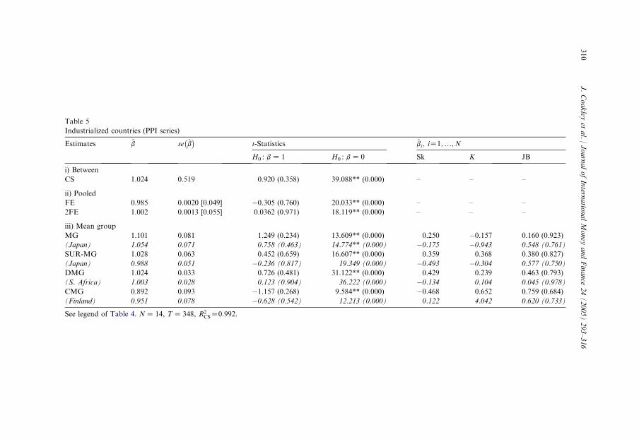
Table 5

Industrialized


bZ 0 Sk K JB

i) Between

CS 88** (0.000) – – –

ii) Pooled

FE 33** (0.000) – – –

2FE 19** (0.000) – – –

iii) Mean grou

MG 09** (0.000) 0.250 �0.157 0.160 (0.923)

(Japan) 74** (0.000) �0.175 �0.943 0.548 (0.761)

SUR-MG 07** (0.000) 0.359 0.368 0.380 (0.827)

(Japan) .349 (0.000) �0.493 �0.304 0.577 (0.750)

DMG 22** (0.000) 0.429 0.239 0.463 (0.793)

(S. Africa) .222 (0.000) �0.134 0.104 0.045 (0.978)

CMG 84** (0.000) �0.468 0.652 0.759 (0.684)

(Finland) .213 (0.000) 0.122 4.042 0.620 (0.733)

See legend of T

310

J.Coakley


atio

nalMoney

andFinance

24(2005)293–316

countries (PPI series)

b se�b�

t-Statistics

H0 : bZ 1 H0 :

1.024 0.519 0.920 (0.358) 39.0

0.985 0.0020 [0.049] �0.305 (0.760) 20.0

1.002 0.0013 [0.055] 0.0362 (0.971) 18.1

p

1.101 0.081 1.249 (0.234) 13.6

1.054 0.071 0.758 (0.463) 14.7

1.028 0.063 0.452 (0.659) 16.6

0.988 0.051 �0.236 (0.817) 19

1.024 0.033 0.726 (0.481) 31.1

1.003 0.028 0.123 (0.904) 36

0.892 0.093 �1.157 (0.268) 9.5

0.951 0.078 �0.628 (0.542) 12

able 4. NZ 14, TZ 348, R2CSZ0:992.

Table 6

Developing c


Z 0 Sk K JB

i) Between

CS ** (0.000) – – –

ii) Pooled

FE ** (0.000) – – –

2FE ** (0.000) – – –

iii) Mean gro

MG ** (0.000) �1.067 3.152 15.700 (0.000)

(2 outliers) 20 (0.000) 1.182 4.391 7.524 (0.023)

SUR-MG ** (0.000) �0.879 2.121 8.222* (0.016)

(3 outliers) ** (0.000) 0.981 0.433 5.652 (0.060)

DMG ** (0.000) 1.590 2.409 17.248** (0.000)

(2 outliers) 03 (0.000) 0.650 0.205 1.730 (0.421)

CMG ** (0.000) �2.249 5.895 59.570** (0.000)

(Sri Lanka) 46 (0.000) �1.124 4.877 8.934 (0.011)

See legend o nmar (MG); India, Malaysia, Myanmar (SUR-MG); El Salvador,

Myanmar (D

311

J.Coakley


atio

nalMoney

andFinance

24(2005)293–316

ountries (CPI series)

b se�b�

t-Statistics

H0 : bZ 1 H0 : b

0.958 0.176 �1.579 (0.114) 36.015

1.001 0.0014 [0.045] 0.022 (0.982) 22.449

0.969 0.0017 [0.054] �0.570 (0.569) 17.822

up

1.101 0.087 1.171 (0.242) 12.732

1.199 0.058 3.431 (0.001) 20.7

1.092 0.085 1.087 (0.277) 12.852

1.153 0.050 3.192 (0.004) 24.000

0.997 0.036 �0.081 (0.935) 27.697

0.956 0.023 �1.881 (0.072) 40.9

0.913 0.133 �0.656 (0.512) 6.874

1.014 0.089 0.159 (0.874) 11.3

f Table 4. NZ 26, TZ 348. R2CSZ0:982. The outliers are Malaysia, Mya

MG).

Table 7

Developing co


: bZ 0 Sk K JB

i) Between

CS .197** (0.000) – – –

ii) Pooled

FE .905** (0.000) – – –

2FE .990** (0.000) – – –

iii) Mean grou

MG .904** (0.000) 2.095 5.669 24.847** (0.000)

(India) 31.697 (0.000) 0.138 0.199 0.053 (0.974)

SUR-MG .566** (0.000) 1.892 3.343 12.746** (0.002)

(India) .178** (0.000) 0.114 0.588 0.182 (0.913)

DMG .923** (0.000) 0.871 1.039 2.057 (0.358)

(Philippines) 63.381 (0.000) �0.527 2.185 0.814 (0.666)

CMG .786** (0.000) �0.518 0.057 0.538 (0.764)

(Egypt) .738** (0.000) 0.313 �1.089 0.724 (0.696)

NZ 12, TZ

312

J.Coakley


atio

nalMoney

andFinance

24(2005)293–316

untries (PPI series)

b se�b�

t-Statistics

H0 : bZ 1 H0

0.937 0.071 �0.887 (0.375) 13

0.985 0.0009 [0.024] �0.623 (0.533) 40

0.972 0.0010 [0.023] �1.238 (0.216) 42

p

1.096 0.061 1.564 (0.118) 17

1.042 0.033 1.288 (0.227)

1.087 0.066 1.322 (0.186) 16

1.028 0.034 0.847 (0.417) 30

0.960 0.021 �1.923 (0.081) 45

0.944 0.015 �3.764 (0.004)

0.889 0.049 �2.214* (0.050) 17

0.923 0.039 �1.987 (0.075) 23

348. See legend of Table 4, R2CSZ0:946.


both industrialized and developing economies (using either CPI or PPI) and thecoefficient is insignificantly different from unity even at the 10% level.17

We report the conventional asymptotic OLS standard errors for the pooledestimates. Since the latter are likely to be downward biased, we also calculatebootstrap standard errors using a procedure that preserves autocorrelation andcross-sectional dependence in the disturbances.18 The OLS standard errors aredwarfed by comparison with those for the MG estimates (discussed below) and morethan 10 times smaller than the bootstrap standard errors.19 The bootstrap t-statisticsstrongly reject the bZ 0 hypothesis and support general relative PPP or bZ 1 in thelong run for all four panels.

One should expect the FE and 2FE estimates to differ markedly when there areunobserved common shocks that are correlated with the regressors. Under theHausman test null, the common shocks are uncorrelated with the regressors and soboth FE and 2FE are consistent but the former is efficient. Under the alternative,only 2FE is consistent.20 For all four panels, the two estimates are insignificantlydifferent which suggests that, if the cross-sectional dependence is induced by latentcommon factors, these are not correlated (or weakly so) with the regressors.

All the MG estimators point in the same direction: the long-run elasticity issignificantly different from zero and insignificantly different from unity. The robustCMG approach provides unambiguous support for long-run PPP on the basis of theInd_PPI and Dev_PPI data sets and borderline support for the Dev_PPI panel.However, the Ind_CPI panel rejects bZ 1 at the 5% level.21 As the averaging issensitive to outliers, we checked for their potential effects in all MG variants byremoving cases for which Z

�bi�hjbi � bMGj=s

bO2 where s

bis the sample standard

deviation of bi; iZ1;.;N. Tables 4–7 report (in italics) the outlier-robust es-timates. The mean group estimates move closer to unity, the associated standarderrors fall and so does the t-ratio in most cases. The outlier-robust CMG estimatorstrengthens the evidence in favour of general relative PPP. More specifically, thet-statistic (bZ 1) for the Dev_PPI panel is now clearly insignificant at the 5% leveladding to the clear-cut evidence for the Ind_PPI and Dev_CPI panels. Therefore, the

17 The support for bZ 1 using the CS estimator is in line with the assumption of strict exogeneity.18 We use a residual-based sieve bootstrap approach that is shown to provide a reasonably good

approximation to the true variability of the FE estimates in the presence of autocorrelated, possibly

non-stationary errors (Fuertes, 2004). The resampling approach is based on pseudo-disturbances that

follow AR(I)MA processes. Cross-section dependence in the residuals is preserved by resampling rows

(t Z 1, 2,.,T ?) with replacement.19 Newey-West standard errors increase only slightly relative to OLS, e.g. at 0.0040 (FE) and 0.0039

(2FE) for the Ind_CPI panel. This is not surprising given that the Newey-West covariance matrix is

inappropriate when the regression errors are I(1) and when cross-section dependence is relevant.20 The test statistic is HZq#

�V�q��1

q. In this case qZbFE � b

2FE, V

�q�ZVðbFEÞ � Vðb2FEÞ and the

squared bootstrap standard errors are used to compute the latter. The p-values from a c2(1) are 0.79

(Ind_CPI), 0.83 (Ind_PPI), 0.74 (Dev_CPI) and 0.68 (Dev_PPI).21 The simulations suggested that the CMG estimator is more efficient in the presence of cross-section

dependence. However, all four panel samples give relatively large CMG standard errors which may reflect

some bias-efficiency trade off resulting from aspects of the true DGP not captured by Eqs. (10)–(13).


deviation of the long-run elasticity from unity suggested by the CMG estimate in theerrant Ind_CPI panel, although significant, may be small in economic terms.

Overall, it seems reasonable to conclude that the long run relative price elasticityis insignificantly different from unity. Nominal exchange rates and price differentialstend to move one-for-one in the long run. How can this finding be reconciled withthe extant literature? The difficulty of testing for long-run relative PPP and hence, themixed to unfavorable evidence in the literature, stems from the fact that the long-runequilibrium real exchange rate may be a moving function of I(1) factors. Oureconometric framework permits testing for general relative PPP when the long-runequilibrium level of the exchange rate is time-varying and subject to permanentshocks.

5. Conclusions

In a log-levels equation relating the nominal exchange rate to the national pricedifferential, general relative PPP implies a long-run unit slope coefficient but norestrictions on the error term. Measurement errors, transaction costs or limits toarbitrage in foreign exchange markets can make the latter appear observationallyequivalent to a unit root sequence. In addition, real exchange rates can be subject totransitory (nominal) or permanent (real) shocks. This paper proposes and imple-ments the first tests of the general relative PPP hypothesis, which posits a long-rununit elasticity of the nominal exchange rate with respect to the price differential, ina robust framework that accommodates shifts in the equilibrium level of the realexchange rate. Simply put, if general relativity holds, then in the long run and otherthings equal, a 1% movement in relative prices will be offset by a commensuratemovement in the nominal exchange rate, and vice versa.

Our work builds on panel estimators that have been shown to be able to identifythe true long-run relationship between non-stationary variables even if they do notcointegrate (Pesaran and Smith, 1995; Phillips and Moon, 1999; Kao, 1999; Coakleyet al., 2001). The intuition is that by pooling or averaging over countries one canattenuate the effect of the noise while retaining the strength of the signal. Severalapproaches are implemented in the empirical analysis in order to capture differentaspects of the panel structure of the data over and above persistent disturbances.These include country heterogeneity and cross-sectional dependence. The finite-sample properties of the panel estimators utilized are analyzed using Monte Carlosimulations.

Cross-sectional dependence may arise from the common variation in the bilateralvalue of the dollar and the US price index (numeraire effect) and, more importantly,from latent global macroeconomic factors that may be correlated with the pricerelative. In this context, a major role is given to inference based on the robustcommon correlated effects estimator recently proposed by Pesaran (2002) to dealwith cross-sectional dependence. The empirical analysis is based on a unique largedataset for 19 industrialized and 26 developing countries, 1970:1–1998:12. Bothinformal graphical analysis and formal statistical tests overall support the hypothesisof a long-run unit price elasticitydi.e. general relativity. We conclude that inflation


differentials are reflected one-for-one in nominal exchange rate depreciation onaverage in the long run. Relative prices matter as PPP posits but it is not just relativeprices that matter. Other (unobservable) non-stationary factors may be responsiblefor the fluctuations of the real exchange rate.

There are further implications of our results that are worth drawing out. The firstis that it may make no sense to speak of speed of adjustment (or half life) toequilibrium in the cointegration sense because the equilibrium is not constant buta moving function of unobserved I(1) factorsdperhaps due to Harrod-Balassa-Samuelson productivity effects, changes in tastes or other real shocks (Bergin et al.,2003; Lothian and Taylor, 2004). Indeed, if this is the case, then empirical measuresof the speed of real exchange rate adjustment that do not account for this shiftingequilibrium will be severely biased towards zerodas the literature on ‘the PPPpuzzle’ attests (Rogoff, 1996). Second, it may be fruitful to analyze further theunderlying economic determinants of this potentially shifting equilibrium to try andidentify it. In this context, it is perhaps comforting thatdas Taylor and Taylor (inpress) notedthe literature has already begun to turn in this direction.

Acknowledgements

This paper was partly written while Mark Taylor was a Visiting Scholar in theResearch Department of the International Monetary Fund. Any views expressed inthe paper are those of the authors alone and do not necessarily represent the viewsof the International Monetary Fund or any of its member countries. An earlierversion of this paper was presented at the Eighth International Conference onMacroeconomic Analysis and International Finance, University of Crete, Rethym-no, 2004. We thank George Kouretas, Bennett McCallum, Michael Melvin,Athanassios Papadopoulos, Lucio Sarno and Ron Smith, as well as the anonymousreferees, for valuable comments on a previous version, although we alone areresponsible for any errors that may remain.

References

Bergin, P.R., Glick, R., Taylor, A.M., 2003. Productivity, tradability, and the great divergence.

Photocopy, University of California, Davis.

Coakley, J., Fuertes, A.M., Smith, R.P., 2001. The effect of I(1) errors in large T, large N panels. Birkbeck

College Discussion Paper in Economics 03/2001 (http://papers.ssrn.com).

Coakley, J., Fuertes, A.M., Smith, R.P., 2002. A principal components approach to cross-section

dependence in panels. Mimeo, Birkbeck College, University of London.

Flood, R.P., Taylor, M.P., 1996. Exchange rate economics: what’s wrong with the conventional macro

approach? In: Frankel, J.A., Galli, G., Giovannini, A. (Eds.), The Microstructure of Foreign Exchange

Markets. Chicago University Press, Chicago.

Frenkel, J.A., 1976. A monetary approach to the exchange rate: doctrinal aspects and empirical evidence.

Scandinavian Journal of Economics 78, 200–224.

Froot, K.A., Rogoff, K., 1995. Perspectives on PPP and long-run real exchange rates. In: Grossman, G.,

Rogoff, K. (Eds.), Handbook of International Economics, vol. 3. Elsevier, North-Holland, Amsterdam;

New York and Oxford.

http://papers.ssrn.com


Fuertes, A.-M., 2004. Robust panel tests for long-run dependence: A sieve bootstrap approach. Mimeo,

Cass Business School.

Granger, C.W.J., Newbold, P., 1974. Spurious regressions in econometrics. Journal of Econometrics 2,

111–120.

Kao, C., 1999. Spurious regression and residual-based tests for cointegration in panel data. Journal of

Econometrics 90, 1–44.

Lothian, J.R., Taylor, M.P., 1997. Real exchange rate behavior: the problem of power and sample size.

Journal of International Money and Finance 16, 945–954.

Lothian, J.R., Taylor, M.P., 2004. Real exchange rates, nonlinearity and relative productivity: The long

and the short of it. University of Warwick, Photocopy.

Officer, L.H., 1982. Purchasing Power Parity and Exchange Rates: Theory, Evidence and Relevance. JAI

Press, Greenwich, Connecticut.

Pesaran, M.H., 2002. Estimation and inference in large heterogeneous panels with cross-section

dependence. Cambridge Working Papers in Economics No. 0305, Faculty of Economics, Cambridge.

Pesaran, M.H., Smith, R., 1995. Estimating long-run relationships from dynamic heterogeneous panels.

Journal of Econometrics 68, 79–113.

Phillips, P.C.B., Moon, H.R., 1999. Linear regression theory for nonstationary panel data. Econometrica

67, 1057–1111.

Rogoff, K., 1996. The purchasing power parity puzzle. Journal of Economic Literature 34, 647–668.

Sarno, L., Taylor, M.P., 2002. Purchasing power parity and the real exchange rate. International

Monetary Fund Staff Papers 49, 65–105.

Taylor, A.M., 2001. Potential pitfalls for the purchasing power parity puzzle? Sampling and specification

biases in mean-reversion tests of the law of one price. Econometrica 69, 473–498.

Taylor, A.M., Taylor, M.P., 2004. The PPP debate. Economic Perspectives 18, 135–158.

Taylor, M.P., 1988. An empirical examination of long-run purchasing power parity using cointegration

techniques. Applied Economics 20, 1369–1381.

Taylor, M.P., 1995. The economics of exchange rates. Journal of Economic Literature 33, 13–47.

Taylor, M.P., Sarno, L., 1998. The behavior of real exchange rates during the post-Bretton Woods period.

Journal of International Economics 46, 281–312.

Documents

Purchasing power parity and the theory of general ... · PDF filePurchasing power parity and the theory of general relativity: the ﬁrst tests Jerry Coakleya, ... (PPP), deﬁned