PUMPED HYDROELECTRIC ENERGY STORAGE … · 2007-12-07 · PUMPED HYDROELECTRIC ENERGY STORAGE AND SPATIAL ... Literature Review ... Overnight capital cost per MW of PHES plant max

PUMPED HYDROELECTRIC ENERGY STORAGE AND SPATIAL DIVERSITY OF WIND RESOURCES AS METHODS OF IMPROVING

UTILIZATION OF RENEWABLE ENERGY SOURCES

Jonah G. Levine B.S., Michigan Technological University, 2003

A thesis submitted to the faculty of the Graduate School of the University of Colorado in partial fulfillment of the requirement for the degree of Master of Science, College of

Engineering and Applied Math December, 2007

ii

Signature Page

This thesis entitled: Pumped Hydroelectric Energy Storage and Spatial Diversity of Wind Resources as Methods of Improving Utilization of Renewable Energy Sources written by Jonah G. Levine has been approved for the Interdisciplinary Telecommunications Program, College of Engineering and Applied Science, University of Colorado at Boulder.

___________________________________________________

Dr. Frank Stevenson Barnes

___________________________________________________ Dr. Michael Hannigan

___________________________________________________ Dr. Patrick Ryan

Date: November 27th 2007

The final copy of this thesis has been examined by the signatories, and we Find that both the content and the form meet acceptable presentation standards

Of scholarly work in the above mentioned discipline.

iii

Abstract Levine, Jonah G (MS. Interdisciplinary Telecommunications Program, College of

Engineering and Applied Science)

Pumped hydroelectric energy storage and spatial diversity of wind resources as

methods of improving the utilization of renewable energy sources

Thesis directed by Distinguished Professor. Frank S Barnes

Renewable energy generation is becoming more prevalent on today’s electric grid.

Part of the challenge of increasing the percentage of renewable energy beyond 20% will be

dealing with the intermittent nature of renewable sources. The following body of work

discusses two methods to integrate intermittent or variable renewable energy in to the electric

system. The methods are pumped hydroelectric energy storage and optimizing the capacity

development of wind generation utilizing complimentary wind regimes encountered with

spatial diversity. The research effort has two general findings.

With regards to pumped hydroelectric energy storage (PHES), Colorado has many

sites with different attributes that could be considered for development. Through PHES

development, Colorado could manage not only its intermittent power generation but facilitate

integration of renewable generation over a much larger geographic region. Opportunities

exist in Colorado to utilize infrastructure already in the ground as well as new construction.

With regards to wind generation, if capacity development is optimized utilizing the

complimentary production encountered with spatial diversity, some percentage of capacity

developed can be utilized as firm power. The analysis herein show 5% of developed capacity

is firm over 99% of the year analyzed. In some cases optimized wind power production

spends 0.00% of time at zero power generation in the given year. Additionally this analysis

may be improved to increase the percentage of capacity which can be counted as firm.

iv

Acknowledgements

The vision and leadership that supported me and this work from start to its current state was Dr. Frank Barnes, thank you Frank. University of Colorado at Boulder’s Energy Storage Research Group received support from the Colorado Energy Research Institute (CERI). Without the generous support of CERI as well as their vision of a more sustainable Colorado this work would not have been possible. Beyond this work the author has gained insight and experience through the reciprocal processes of working, teaching, and learning that will enable not just a better understanding of pumped storage but a stronger grasp of the challenge and potential solutions that are precipitated by intermittent energy generation. Thank you CERI. University of Colorado at Boulder’s Energy Storage Research Group received support from the Colorado Department of Agriculture. This support enabled the study of small scale distributed energy storage applicable to family farm scale applications. University of Colorado at Boulder’s Energy Storage Research Group received support from University of Colorado’s Energy Initiative. This support directly funded the following thesis by supporting the study of potential locations for development of PHES in Colorado. This support also facilitated legal analysis of water and regulatory right relevant to this work. University of Colorado at Boulder’s Energy Storage Research Group received regular collaboration and working support from University of Colorado School of Law’s Energy and Environmental Security Initiative (EESI). The intellectual collaboration between the disciplines of engineering and law bring technical ideas closer to political fruition. Thank you EESI. Rocky Mountain Institute with support from the Argosy Foundation were helpful in my learning process while this work was developed. Ms. Lena Hansen provided a great deal of intellectual capital around quantifying the results of spatial diversity and optimization of wind power. Together with Lena I look forward to further developing this body of work.

v

Table of Contents 1. Introduction................................................................................................................1 2. Pumped Hydroelectric Energy Storage in Colorado .................................................4

2.1. Background and Literature Review........................................................................4 2.2. Methods...............................................................................................................10

2.2.1. Power and Capacity.....................................................................................11 2.2.2. Revenue .......................................................................................................12 2.2.3. Energy Purchase and Sales Differential .......................................................13 2.2.4. Avoided Peak Generation Cost.....................................................................14 2.2.5. CO2 value & SO2 value ................................................................................15 2.2.6. Cost .............................................................................................................16 2.2.7. Payback .......................................................................................................17

2.3. Results and Discussion of PHES Sites in Colorado ..............................................19 2.3.1. New Management of Imbedded Infrastructure ..............................................19 2.3.2. New infrastructure .......................................................................................23

2.4. Conclusions Next Steps........................................................................................46 3. Spatial Diversity Optimization of Wind Capacity Development.............................50

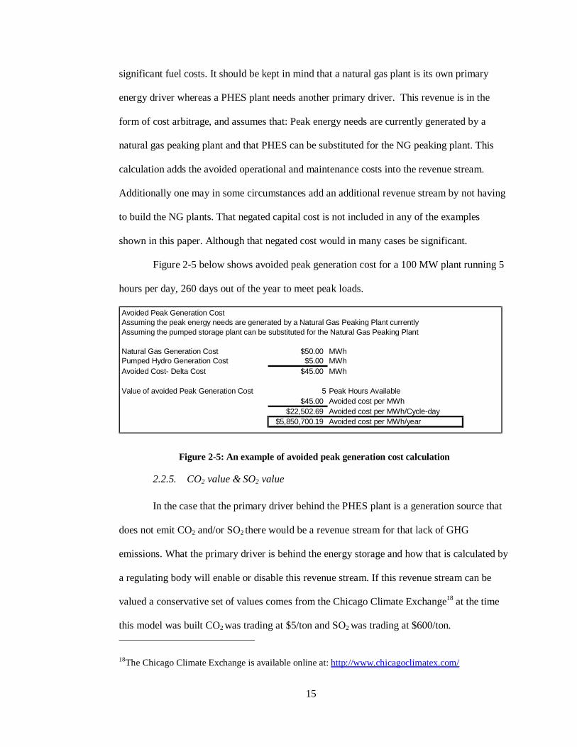
3.1. Background .........................................................................................................50 a. Literature Review ............................................................................................51

3.2. Methods...............................................................................................................54 a. Data Collection ...............................................................................................54 3.2.1. Data Choice.................................................................................................56 3.2.2. Power Production Model .............................................................................58

3.3. Results & Discussion ...........................................................................................65 a. Data Collection ...............................................................................................65 b. Data Choice.....................................................................................................65 c. Power Production Model and Optimization .........................................................65

3.4. Conclusions and Next Steps .................................................................................77 4. A spatially optimized and PHES integrated wind energy system ...........................79

vi

Table of Figures

Figure 2-1: Seven Days of Wind Generation and Loads.........................................................4 Figure 2-2: Increasing system cost over increasing penetration of wind power on Xcel Energy’s electric grid. ...........................................................................................................6 Figure 2-3: A basic schematic of the pumped hydro installation at Raccoon Mountain...........7 Figure 2-4: kWh sales and purchase differential ..................................................................14 Figure 2-5: An example of avoided peak generation cost calculation ...................................15 Figure 2-6: CO2 and SO2 emissions reduction value example calculation .............................16 Figure 2-7: Cabin Creek as Calculated technical and economic output.................................25 Figure 2-8: Bellyache Ridge................................................................................................27 Figure 2-9: Payback period sensitivity analysis with changing kWh price margin ................29 Figure 2-10: View of the West Gypsum Potential Site; 1-Aproxamate forebay location, 2-Afterbay may be located anywhere along the Eagle River I-70 corridor to facilitate siting. Eagle River I-70 corridor is marked in a bold black line. .....................................................29 Figure 2-11: West Gypsum Technical and Economic Summary Output ...............................30 Figure 2-12: View of Horsetooth reservoir and College Lake on the western edge of Ft Collins Colorado and the CSU campus................................................................................31 Figure 2-13: Horsetooth reservoir and College Lake............................................................32 Figure 2-14: David Pt technical and economic output ..........................................................35 Figure 2-15: Schoolhouse Pt technical and economic output................................................37 Figure 2-16: Peetz Bluffs technical and economic output.....................................................39 Figure 2-17: Gunnison Hydro Blue Mesa technical and economic output ............................41 Figure 2-18 White River technical and economic output......................................................43 Figure 2-19: S2 Cathedral technical and economic output....................................................45 Figure 2-20: Overhead view of S2 Cathedral .......................................................................46 Figure 3-1: Available data sets refering to distinct data recording locations per year ...........56 Figure 3-2: Diversity of data locations by power pool..........................................................57 Figure 3-3: Diversity of data site locations by state..............................................................58 Figure 3-4: Power curve for a V80- 2.0 MW at 1.22kg/m^2 air density ...............................63 Figure 3-5: Power output of five locations in Texas, Jan 1st 2004........................................67 Figure 3-6: Texas system mean variance frontier .................................................................68 Figure 3-7: Optimized output of the Texas system on Jan 1st 2004......................................69 Figure 3-8: 2004 Texas system output histogram optimized to produce 400kW as a minimum portfolio output ...................................................................................................................70 Figure 3-9: 2004 optimized Minnesota wind system............................................................72 Figure 3-10: 2004 optimized North Dakota wind system .....................................................73 Figure 3-11: 2004 optimized MRO wind system, which includes both Minnesota and North Dakota ................................................................................................................................75 Figure 3-12: 2004 optimized Kansas wind system ...............................................................76 Figure 4-1: Sweetwater Texas 2004 power output ...............................................................80 Figure 4-2: Texas wind system optimized to decrease variability utilizing spatial distribution...........................................................................................................................................81 Figure 4-3: Texas wind system optimized to decrease variability utilizing spatial distribution and 10% capacity of PHES .................................................................................................81 Figure 4-4: Texas wind system optimized to decrease variability utilizing spatial distribution and 20% capacity of PHES .................................................................................................82 Figure 4-5: Texas wind system optimized to decrease variability utilizing spatial distribution and 30% capacity of PHES .................................................................................................83

vii

List of Tables Table 2-1: Gas Cost Impact of wind penetrations with and without storage on Xcel’s electric grid.......................................................................................................................................5 Table 2-2: Cost impact of increasing wind penetration on Xcel’s electric grid .......................5 Table 2-3: Overnight capital cost per MW of PHES plant max rated size.............................17 Table 2-4: Constituent costs of a PHES plant as a percent of the total overnight capital cost estimate ..............................................................................................................................17 Table 2-5: PHES in Colorado with Developed or Partially Developed Infrastructure ...........19 Table 2-6: A sampling of new infrastructure PHES sites in Colorado ..................................23 Table 3-1: Number of data sets in each of the power pools available by year .......................57 Table 3-2: Assumed air density based on elevation..............................................................61 Table 3-3: Power production output for five Texas locations on a Vestas V80-2MW...........66 Table 3-4: System reliability percentage at x percent of capacity .........................................71 Table 3-5: Minnesota 2004 reliability percent as a percentage of total capacity when optimized............................................................................................................................72 Table 3-6: North Dakota 2004 reliability percent as a percentage of total capacity when optimized............................................................................................................................73 Table 3-7: Midwest reliability organization 2004 reliability percent as a percentage of total capacity when optimized.....................................................................................................75 Table 3-8: Kansas 2004 reliability percent as a percentage of total capacity when optimized76

1

1. Introduction


While Colorado’s political atmosphere is driving changes in our electric utility industry, the

industry is hesitant to change how it has been supplying reliable electric power for nearly a

century. Some of the reason for this hesitation is the intermittent or variable nature of

renewable sources. For instance, solar electricity is not going to function at night, and

likewise wind generation will not generate electricity when the wind is not blowing. This

variable energy manifests the challenge times when no output is available, and times when

excess output is generated. Additionally, other challenges arise such as momentary faults and

decreased ability to manage the real versus reactive power on the electric system. This set of

challenges can be classified generally as variable or intermittent generation integration issues.

One part of solving the intermittent integration challenge is electrical energy storage.

An effort has been successful increasing the amount of renewable energy in Colorado

by raising the current Renewable Portfolio Standard (RPS) from 10% to 20% renewable

source generation by the year 2020. This will bring with it both technical and economic

consequences. Some positive consequences include bolstering clean energy industries in

Colorado, diversifying our generation portfolio, and protecting our environment. Part of the

challenge of increasing the percentage of renewable energy (to 20% penetration and beyond)

will be dealing with the intermittent nature of renewable sources. Increasing the amount of

intermittent sources without ensuring they are available when needed still requires the capital

cost investment in conventional generation plants. The net result is an unnecessarily

increased cost for electric power. If legislation encourages system wide planning to ensure

energy is available when it is needed while minimizing the externalities of fossil fuel

generation and maintaining reasonable cost, Colorado has the opportunity to set a positive

example of energy systems planning.

2

What can be done to solve the challenge presented by the need for energy when

renewable production is not available? Or conversely, what can be done to handle excess

energy created when intermittent generation is high and demand is low? The most effective

solution will be an integrated approach, which should include:

1. Diversifying the types and locations of renewable generation sources. This method

should be an optimization of spatial diversity and renewable generation sources that

minimizes intermittence and cost while maximizing capacity to meet or exceed RPS

targets while meeting loads with over 99% reliability.

2. Encouraging demand side management (DSM) to serve as a renewable source of

energy, this can be thought of as virtual base load generation many times referred to

as the negawatt. DSM can also be used to describe the deployment or control of

loads.

3. Developing adequate transmission infrastructure to facilitate diversified renewable

plant locations.

4. Planning for additional energy storage on Colorado’s electric grid that optimizes the

utilization of transmission and generation resources minimizing costs and green

house gas (GHG) emissions, and allows renewable energy to be dispatched with

more flexibility.

5. Formulate legislation that provides incentives for the first four points.

None of the above points are silver bullets to facilitate 20% and greater penetration of

renewable power sources. Moreover, if only one of the above strategies is pursued it will be

less valuable than if a combination are pursued. Each point will increase the reliability of

Colorado’s electric grid and have synergistically positive effects on the other points. One

alternative to the above mitigating steps is building additional peaking natural gas plants to

provide on demand energy in the absence of sun and wind, though this is seemingly contrary

to an increased RPS.

3

Evaluating both the technical and economic ramifications of each of the five

mitigating steps will need to be done as efforts move forward with RPS deployment. It is

evident that a system analysis for the state as a whole or a larger geographic region will need

to be conducted to determine the most effective solution to the challenges poised by

intermittent power generation. Legislation needs to be written so that those generating,

transmitting and distributing the energy have incentives to optimize the system as a whole.

This optimization will enable renewable energy sources to meet as large a fraction as possible

of the public’s need for reliable power, while concurrently setting the stage for increasing

Colorado’s renewable generation beyond 20%. To this end, the following body of work will

draw on current knowledge and propose future projects to facilitate the integration of

intermittent power on to the electric grid.

This thesis will be presented in two major parts. Chapter II deals with the potential

for deployment of pumped hydroelectric energy storage (PHES) resources in the state. It

includes site analysis of various potential locations for PHES around the state. These sites

are analyzed using a model developed to determine expected physical and financial aspects of

the sites. Chapter III deals with the optimization of wind generating resources via spatial

diversity of the wind generators.

4

2. Pumped Hydroelectric Energy Storage in Colorado

2.1. Background and Literature Review


Colorado voters have passed and state legislators have recently increased required renewable

generation targets (via our RPS, Amendment 37) for the most significant independent system

operators (ISO’s), municipal suppliers (MUNI’s), and rural electric associations (REA’s) in

the State. One method for solving the intermittent challenge is electrical energy storage.

Figure 2-1 displays the fundamental problem by plotting both a daily load profile and a wind

generation profile.

Seven Days Of Loads From One Municipality Assuming Peak Consumption & Seven Days of Wind Generation From the Same Region.

0.00

50.00

100.00

150.00

200.00

250.00

300.00

0 24 48 72 96 120 144 168

Hour

Pow

er[M

W]

Winter '05/'06 City Peak (MW)Summer '06 City Peak (MW)Wind Generation[MW]

Figure 2-1: Seven Days of Wind Generation and Loads.

The non-zero magnitudes of wind generation can be increased by building additional

wind capacity, essentially multiplying current energy generated by the added resource.

However, multiplying the zero values by any additional generation will continue to yield a

zero energy result. Many of those zero energy time periods align with loads that need to be

met. Energy storage and optimization of generation capacity development are fundamental

5

steps in solving the intermittent generation challenge. Electrical energy storage addresses the

following aspects of system operation:1

1. Dispatchability- Responding to fluctuations in electricity demand.

2. Efficiency- Recovering wasted energy.

3. Regulatory-driven needs- meeting distribution and other transmission capacity

expansion requirements.

As the penetration percent of intermittent generation grows on Colorado’s electric

grid, the need for energy storage to augment electricity generation will become increasingly

acute. It was recently shown by Xcel Energy that at and above 20% intermittent generation

on Xcel’s grid significant economic cost increases will manifest2 if mitigation techniques are

not pursued. With regard to Xcel Energy’s electric grid one study points out the cost to

integrate renewable generation is as shown in Table 2-1, Table 2-2 and Figure 2-2:

Table 2-1: Gas Cost Impact of wind penetrations with and without storage on Xcel’s electric grid

Wind Penetration 10% 15% $/MWH Gas Impact No Storage Benefits $2.17 $2.52 $/MWH Gas Impact with storage benefits $1.26 $1.45

Table 2-2: Cost impact of increasing wind penetration on Xcel’s electric grid

Wind Penetration

Electric Production Cost Impact

Gas Supply System Impact

Total

10% $2.25 $1.26 $3.51/MWH 15% $3.32 $1.45 $4.77/MWH 20% $7.47 $2.10 $9.57/MWH

1 Tester. 2005. Chapter 16 Storage, Transportation, and Distribution of Energy in, Sustainable Energy Choosing among Options.I ed., vol. 1, S. Howe, Ed. Cambridge, Massachusetts: The MIT Press. PP 648, 648-686. 2 Oakleaf. RMEL 2006 Renewables Conference: New Developments in Applications. Nov 29, 2006. http://www.rmel.org

http://www.rmel.org

6

Cost/MWh System Impact at Increasing Penetration % Wind Power

$0.00

$2.00

$4.00

$6.00

$8.00

$10.00

$12.00

5% 10% 15% 20% 25%

Penetration % of Wind Power

$/M

Wh

Cos

t Inc

reas

e ...

.....

Electric Production CostIncreaseGas Supply System Impact

Total Cost Impact

Figure 2-2: Increasing system cost over increasing penetration of wind power on Xcel Energy’s electric grid.

Figure 2-2 shows an increasing cost of electric energy over an increasing penetration

of wind power. This increasing cost has 324 MW of pumped storage available on the system

which illustrates the effect of the increasing costs. Table 2-1 shows that natural gas cost

increases will take place without the use of energy storage on the system.

Pumped hydroelectric energy storage (PHES) is a mature technology that has been

deployed for over a century.3 Examples of installed PHES systems as early as 1890 can be

found in both Italy and Switzerland. PHES does not generate electricity, rather is a storage

mechanism.4 PHES uses electricity to pump water uphill to be stored, then energy is later

recaptured when the water released back down hill through a turbine PHES systems are

highly efficient, capable of reaching and surpassing 80-85% round-trip efficiencies. The

3Lawrence. 2006. Hydropower. Lecture noteSYST6820(2006)online http://leeds-faculty.colorado.edu/Lawrence/SYST6820/Lectures/Hydropower.ppt 4 In the case that the forebay collects precipitation in its natural watershed via drainage the power generated is generation because it has not been pumped. This scenario is a very small amount of the total capacity of any PHES unit.

7

scale of PHES this paper addresses is suited to the functional ability of the Francis turbine.5

The Francis turbine is capable of reversible operation, utilizing a single unit that acts as a

motor-pump or a turbine-generator. Figure 2-3 shows a basic schematic of the PHES

installation at Raccoon Mountain owned and operated by the Tennessee Valley Authority

(TVA).

Figure 2-3: A basic schematic of the pumped hydro installation at Raccoon Mountain

The Raccoon Mountain Pumped-Storage Plant6 is a widely cited example of PHES.

Plant construction began in 1970 and was complete in 1978. The generating capacity of

Raccoon Mountain is about 1,600 megawatts and it can run for 22 hours to supply 35,200

MWh of electricity.

5 J. W. Tester, “Chapter 12 Hydropower.” in, Sustainable Energy Choosing among Options ,I ed., vol. 1, S. Howe, Ed. Cambridge, Massachusetts: The MIT Press, 2005, pp. 529. 6 More information for Raccoon Mountain can be found at http://www.tva.gov/sites/raccoonmt.htm

http://www.tva.gov/sites/raccoonmt.htm

8

Armstrong and Mermel in 19747 compiled a series of papers from a conference into a

text titled Converting Existing Hydro-Electric Dams and Reservoirs into Pumped Storage

Facilities. This text is valuable in covering many topics including sections on siting potential,

equipment, innovations, construction, and environmental problems and solutions.

Wood and Wollenberg in 19968 published a text titled Power Generation, Operation,

and Control this text covers operational techniques for power generation including pumped

hydroelectric plants (page 230).

Stone and Webster Consultants in December of 19889 put out a report titled Colorado

Joint Planning Study Economic Potential of Pumped Storage. This report defines the

expected loads and the generation needed to meet those loads. It explores the potential of

pumped storage to facilitate future planning as well as the timing the deployment of PHES

resources.

The US Department of Interior Bureau of Reclamation has a number of older

documents on this topic. Web based resources for the Bureau are referenced throughout this

document but two resources of note are: Wind-hydroelectric Energy project- Wyoming10,

September 1984. This document looks at a wind and hydroelectric integrated project but does

not make any significant conclusion due to difficulties with the wind machines at the time of

the study. The second document of note is entitled: Potential Power Additions To The

7 Armstrong E. Mermel T. 1974. Converting Existing Hydro-Electric Dams and Reservoirs into Pumped Storage Facilities. American Society of Civil Engineers. New York, NY. 8 Wood A. Wollenberg B. 1996. Power Generation, Operation, and Control. Wiley-Interscience Publication, John Wiley and Sons, Inc. New York NY. 9 Stone & Webster Management Consultants. 1988. Colorado Joint Planning Study Economic Potential of Pumped Storage. Colorado, Denver 10 US Department of the Interior Bureau of Reclamation. 1984. Wind Hydroelectric Energy Project Wyoming: Status Report on System Verification Units.

9

Colorado-Big Thompson Project Pick-Sloan Missouri Basin Program Colorado11 published

in 1978. This document covers a potential PHES location on the Colorado Big Thompson

Project.

Dr. David Harpman with the Bureau of reclamation has contributed to this pool of

knowledge through a number of efforts. Some of his work can be seen at his web site at:

http://mysite.du.edu/~dharpman/profdownload.html. Included at this website is a paper titled

Exploring the Economic Value of Hydropower in the Interconnected Electricity System.12

This paper was influential in quantification of ancillary services in the following pumped

hydroelectric economic modeling.

Chiu, L Et Al wrote Mechanical Energy Storage Systems: Compressed Air and

Underground Pumped Hydro in 1978.13 This paper looks at the costs for development of

CAES as well as underground PHES. This work was presented at an AIAA meeting in

Alabama in January, 1978.

Bueno and Carta wrote Wind Powered Pumped Hydro Storage Systems, a means of

increasing the penetration of renewable energy in the Canary Islands in 2006.14 This paper

looks at the sizing of a PHES application to meet the needs of a specific island energy

system.

11 US Department of the Interior Bureau of Reclamation. April 1978. Potential Power Additions To The Colorado-Big Thompson Project Pick-Sloan Missouri Basin Program Colorado 12 Harpman D. 2006. Exploring the Economic Value of Hydropower in the Interconnected electricity System. Available online at: http://mysite.du.edu/~dharpman/profdownload.html. Also available from NTIS 13 Chiu, L Et Al. 1978. Mechanical Energy Storage Systems: Compressed Air and Underground Pumped Hydro. AIAA. Huntsville Alabama. 14 Buena C. Carta J. October 2006. Wind powered pumped hydro storage systems, a means of increasing the penetration of renewable energy in the Canary Islands. Renewable and Sustainable Energy Reviews. 312-340

http://mysite.du.edu/~dharpman/profdownload.html


10

Between 2005 and 2006, Van Kooten et. al. have produced a series of papers looking

at the dynamic between different generation and storage resources on the grid versus the

increasing penetrations of renewable energy.15 16 17

2.2. Methods

To address the potential for PHES systems in Colorado, locations had to be identified

and then assessed for their technical and economic applicability. The methods for this

analysis were designed to be able to assess multiple sites around the state at a high level. If

further interest is sparked in any of the sites suggested in this body of work, a more detailed

analysis should be performed.

To identify locations for PHES additions in Colorado, locations were looked for that

utilized infrastructure already in the ground. To this end, US Bureau of Reclamation (USBR)

hydro projects in Colorado were surveyed. Those projects are the Colorado Big Thompson

and the Frying Pan Arkansas. Additionally a meeting was held with the Senior Power Liaison

Mr. Michael Roluti, of the US Department of Interior Bureau of Reclamation to discuss

PHES potential on the USBR system. After the USBR projects were surveyed PHES sites

were looked for that had good characteristics for development. Favorable site characteristics

include:

15P. Benitez, L. Dragulescu and C. Van Kooten. (2006). "The Economics of Wind Power with Energy Storage," Resource and Environmental Economics and Policy Analysis (REPA) Research Group, pp. 1-38, 2006.

16 P. Lawrence, G. Cornelis van Kooten, Murray Love and Ned Djilali, "Utility-Scale Wind Power: Impacts of Increased Penetration": Paper No. IGEC-097 in Proceedings of the International Green Energy Conference, June 12-16, 2005, Waterloo, Ontario, Canada.

17Liu, Jia, G. Cornelis van Kooten and Lawrence Pitt. June 2005. Integrating Wind Power in Electricity Grids: An Economic Analysis. Paper No. IGEC-1-017 in Proceedings of the International Green Energy Conference. Waterloo, Ontario, Canada. Available: http://www.iesvic.uvic.ca/publications/library/IGEC_Pitt.pdf

http://www.iesvic.uvic.ca/publications/library/IGEC_Pitt.pdf

11

• High head potential

• Water availability

• Areas conducive for forebay and afterbay construction or utilization

• Adjacent to transmission or distribution lines

• Utility right of ways

• Renewable generation development

• Strong wind or solar potential

• A road

A model has been developed that analyzes both economic and technical

characteristics of each site. This model is run in a series of tabs in a Microsoft Excel

workbook. The tabs are as follows:

1. Power and Capacity

2. Revenue

3. Cost

4. Payback

2.2.1. Power and Capacity

To calculate the technical specifications of a pumped hydroelectric site, a basic fluid

power equation is used. The inputs to the equation that change based on the location are head,

flow, and efficiency. Head is given by the upper elevation minus the lower elevation. A more

in-depth feasibility study of PHES would specify the effective head, and effective head is not

given in this work. Effective head is the elevation differential adjusted to account for

efficiency. The flow rate in this analysis can be entered in one of two ways. Most of the sites

in this analysis have flow dictated by the expected volumetric area of the limiting reservoir

divided by the desired storage time to yield the available flow, minus a 15% reservoir

12

operating cushion. If water ways are already in place or there is another reason flow rate is

known, that flow rate can be directly entered into the calculator.

Given hydraulic head, an upper bound on flow rate, and efficiency of the plant, the

power generation capacity of a pumped hydroelectric installation can be calculated with the

following equation:

Next, given the power capacity of the plant, the limiting volume of the upper or lower

reservoir dictates the energy capacity. Potential energy generation or kilowatt hours [kWh]

are calculated by power output multiplied by run time. Run time is a function of flow rate and

reservoir volume.

2.2.2. Revenue

Revenue is calculated as described in this section. Power as well as energy are

imported as a link from the power and capacity page of the model worksheet. The revenue is

calculated via multiple revenue streams:

1. kWh purchase and sales differential

2. Avoided peak generation cost

3. CO2 value

4. SO2 value

P = Q ⋅ H ⋅ ρ ⋅ g ⋅η

Where P = generated output power in Watts [W]

Q = fluid flow in cubic meters per second [m3/s]

ρ = fluid density in kilograms per cubic meter [kg/m3] = 1000 [kg/m3] for water

H = hydraulic head height in meters [m]

g = acceleration due to gravity [m/s2] = 9.81 [m/s2]

η = efficiency

13

Other revenue streams do exist and may be viable contributions to these projects although

they will not always apply and have not been included here. These other steams include

ancillary services, transmission development deferral, capital cost deferral for other types of

fast response plants, capacity values and a multitude of revenue streams associated with the

storage of water.

2.2.3. Energy Purchase and Sales Differential

PHES must pull energy from the grid and then return energy to the grid when it is

called for. Efficiency losses will mean that approximately 20% of the energy pumped into the

system will be lost and not returned out of the system. But, due to the fact that during peak

demand times or other times when energy is lacking (such as a situation where the wind

power drops off) the value of a kWh increases. Thus, the efficiency loss per kWh can be

compensated financially by a higher value for the timely delivery of that next unit of energy.

If energy costs $0.03 kWh and the energy is sold for $0.13 kWh with an 80% round trip

efficiency, the kWh differential is $0.08. If a PHES plant is rated at 100 MW and can run for

5 hours per day, that day with the differential described above would yield:

(($0.13 * 100,000kW * 5 hours) - ($0.03 * 100,000kW * 5 hours)) * 0.80 =

$40,000.00.

In the case that this cycle would run 5 days per week and 52 weeks per year, the annual value

of the kWh differential would be:

$40,000.00/revenue cycle * 5day/week * 52weeks/year = $10,400,000.00 annual

kWh purchase and sales differential

Unfortunately kWh revenue streams do not work out that simply. In a functioning

energy market the purchase price and the sales price fluctuate with the market. This is a basic

function of supply and demand. The model calculates kWh differential by varying the both

the purchase price and the sales price of the kWh over time of day. When the demand is high

14

the value of the kWh is high and when the demand is low the value of the kWh is low. The

model uses a set of nested if/then statements to make the decision to purchase when the cost

is lowest and sell when the price is highest. These choices are kept within the constraints of

the system. The constraints of the system force the PHES plant to run a full cycle of all

dispatchable energy but do not allow the system to over-pump the capacity of either reservoir.

The model also requires that the days per week and weeks per year the system will function

be specified by the user. A typical output for kWh purchase and sales differential is displayed

below in Figure 2-4:

Hours hourly value action rating action unit cost Logic kWh Sales-Gen Sales-Gen Value Logic kWh Buy-Pump Cost Value0 0.0368 BUY 4 -0.0368 0 0 $0.00 1 374518 -$13,787.251 0.0343 BUY 3 -0.0343 0 0 $0.00 1 374518 -$12,852.622 0.0328 BUY 2 -0.0328 0 0 $0.00 1 374518 -$12,269.203 0.0316 BUY 1 -0.0316 0 0 $0.00 1 374518 -$11,846.414 0.0429 BUY 5 -0.0429 0 0 $0.00 1 374518 -$16,048.655 0.0433 BUY 6 -0.0433 0 0 $0.00 1 374518 -$16,205.276 0.0541 BUY 7 -0.0541 0 0 $0.00 1 374518 -$20,245.367 0.0608 BUY 8 -0.0608 0 0 $0.00 1 374518 -$22,774.698 0.0676 IDLE 10 0.0000 0 0 $0.00 0 0 $0.009 0.0710 IDLE 11 0.0000 0 0 $0.00 0 0 $0.0010 0.0769 IDLE 13 0.0000 0 0 $0.00 0 0 $0.0011 0.0823 IDLE 14 0.0000 0 0 $0.00 0 0 $0.0012 0.0860 IDLE 17 0.0000 0 0 $0.00 0 0 $0.0013 0.0876 SELL 18 0.0876 1 374517.7714 $32,802.59 0 0 $0.0014 0.1034 SELL 20 0.1034 1 374517.7714 $38,729.46 0 0 $0.0015 0.1058 SELL 23 0.1058 1 374517.7714 $39,631.18 0 0 $0.0016 0.1100 SELL 24 0.1100 1 374517.7714 $41,196.95 0 0 $0.0017 0.1043 SELL 21 0.1043 1 374517.7714 $39,050.68 0 0 $0.0018 0.1050 SELL 22 0.1050 1 374517.7714 $39,324.37 0 0 $0.0019 0.0943 SELL 19 0.0943 1 374517.7714 $35,334.31 0 0 $0.0020 0.0834 IDLE 16 0.0000 0 0 $0.00 0 0 $0.0021 0.0827 IDLE 15 0.0000 0 0 $0.00 0 0 $0.0022 0.0722 IDLE 12 0.0000 0 0 $0.00 0 0 $0.0023 0.0624 BUY 9 -0.0624 0 0 $0.00 0.4 149807 -$9,344.75

SUM 0.3115 7 2621624.4 $266,069.54 8.4 3145949 -$135,374.21374518

CYCLE REV $130,695.33

Figure 2-4: kWh sales and purchase differential

The equation for kWh differential revenue generation is as follows:

(kWh sales value * power * time at that value and power) - (kWh cost value * power

* time at that value and power) * Efficiency of the plant = kWh differential value

2.2.4. Avoided Peak Generation Cost

Peak generation costs are costs avoided by running a PHES plant rather than running

a Natural Gas Peaking plant (NG). The most significant cost difference between a PHES

plant and an NG plant is that a PHES does not have a fuel cost where NG plants have

15

significant fuel costs. It should be kept in mind that a natural gas plant is its own primary

energy driver whereas a PHES plant needs another primary driver. This revenue is in the

form of cost arbitrage, and assumes that: Peak energy needs are currently generated by a

natural gas peaking plant and that PHES can be substituted for the NG peaking plant. This

calculation adds the avoided operational and maintenance costs into the revenue stream.

Additionally one may in some circumstances add an additional revenue stream by not having

to build the NG plants. That negated capital cost is not included in any of the examples

shown in this paper. Although that negated cost would in many cases be significant.

Figure 2-5 below shows avoided peak generation cost for a 100 MW plant running 5

hours per day, 260 days out of the year to meet peak loads.

Avoided Peak Generation CostAssuming the peak energy needs are generated by a Natural Gas Peaking Plant currentlyAssuming the pumped storage plant can be substituted for the Natural Gas Peaking Plant

Natural Gas Generation Cost $50.00 MWhPumped Hydro Generation Cost $5.00 MWhAvoided Cost- Delta Cost $45.00 MWh

Value of avoided Peak Generation Cost 5 Peak Hours Available$45.00 Avoided cost per MWh

$22,502.69 Avoided cost per MWh/Cycle-day$5,850,700.19 Avoided cost per MWh/year

Figure 2-5: An example of avoided peak generation cost calculation

2.2.5. CO2 value & SO2 value

In the case that the primary driver behind the PHES plant is a generation source that

does not emit CO2 and/or SO2 there would be a revenue stream for that lack of GHG

emissions. What the primary driver is behind the energy storage and how that is calculated by

a regulating body will enable or disable this revenue stream. If this revenue stream can be

valued a conservative set of values comes from the Chicago Climate Exchange18 at the time

this model was built CO2 was trading at $5/ton and SO2 was trading at $600/ton.

18The Chicago Climate Exchange is available online at: http://www.chicagoclimatex.com/

http://www.chicagoclimatex.com/

16

Figure 2-6 below shows an emissions reduction value of CO2 and SO2 as traded on

the Chicago Climate Exchange for a 100 MW plant running 5 hours per day, 260 days out of

the year. This reduction was only calculated for the NG peaking plant not running. Other

reductions would be expected as the PHES plant would allow additional wind and solar

energy onto the grid due to the economic boost of a firm resource and dispatchability attained

through the PHES infrastructure.

Avoided EmissionsThe following calculations show the avoided emissions by utilizing pumped hydro in the place of NG Peaking Plants

CO2

Assuming NG Peaking Plant Produces 2,377.40 lbs CO2/MWhAssuming pumped hydro plant produces 0.00 lbs CO2/MWhavoided co2 2,377.40 lbs CO2/MWhEnergy Produced 500.06 MWh produced/cyclelbs CO2 avoided per cycle 1,188,842.28 lbs CO2 avoided per cyclelbs CO2 avoided per year 140,204.98 tons[metric] of CO2 avoided/yearvalue of CO2 $5.00 value per ton CO2

value of avoided CO2 $701,024.92 value per annual CO2 reduction

SO2

Assuming NG Peaking Plant Produces 0.53 lbs SO2/MWhAssuming pumped hydro plant produces 0.00 lbs SO2/MWhavoided SO2 0.53 lbs SO2/MWhEnergy Produced 500.06 MWh produced/cyclelbs SO2 avoided per cycle 265.03 lbs SO2 avoided per cyclelbs SO2 avoided per year 31.26 tons[metric] of SO2 avoided/yearValue per Metric Ton SO2 $600.00 $/metric tonAnnual Value $18,753.76 Annual Traded Value

Figure 2-6: CO2 and SO2 emissions reduction value example calculation

2.2.6. Cost

The capital cost determined by the model for each potential PHES site is calculated

with an overnight cost estimate. That estimate scales down in capital cost as the capacity of a

plant scales up. Additionally, the overnight capital cost is broken out into constituent costs of

bringing a plant online. Table 2-3 displays the overnight capital cost per MW of power as it

scales with size. Table 2-4 breaks out the constituent costs of a plant as a percent of those

17

total costs. In the case that a potential site will not need any individual cost of the eight costs

broken out, those costs can be removed from the calculation by a function in the model.

Table 2-3: Overnight capital cost per MW of PHES plant max rated size

Sizing of Plant Overnight Cost

Mini < 1MW $5,000,000 $/MW Small >1MW, < 10 MW $3,500,000 $/MW Medium >10MW, < 50 MW $2,500,000 $/MW Large >50MW, <200 MW $1,800,000 $/MW Extra Large >200 MW $1,300,000 $/MW

Table 2-4: Constituent costs of a PHES plant as a percent of the total overnight capital cost estimate

Item % of Capital Cost land and land rights 2.05% Power Station structures and improvements

8.73%

Reservoirs and Water Ways 22.15% Pumps Turbines Valves Governors

9.22%

Generator Motors and Static Starting Equipment

6.40%

Accessory Electrical Power plant Substation Equipment, Roads

10.17%

Contingencies Engineering and Overhead 14.16% Allowance for funds during construction 27.12% TOTAL 100.00%

2.2.7. Payback

A time valued payback is used as the metric by which these PHES sites are fiscally

measured. Each of the revenue streams as well as each of the costs described in this body of

work can be valued or not valued within the model. The payback tab drives out the capital

costs with an interest rate over specified period of construction. During the specified period

of construction no revenues are garnered although interest accrues. When the construction

period passes the annual revenue starts paying back the financed balance. Operation and

management (O and M) costs are figured at ½ of one percent of the initial capital cost per

18

year. In the case of a 200 MW plant the capital cost would be calculated at 1.3 million dollars

per MW for a total of 260 million dollars. That hypothetical 200 MW plant would have an

annual O and M budget of 1.3 million dollars. Additionally, an annual percentage increase in

costs and revenues in assumed (typically 1%). The annual percentage increase will affect the

O and M cost and the revenue streams.

The payback model functions in the following order. First, capital costs are brought

into the model. Second, the financed capital costs are divided over the specified years of

construction. Third, after the completion of construction, O and M costs as well as revenues

begin to run at the plant on an annual or otherwise specified periodic basis. Each period the

revenue streams are first applied to the O and M costs, then the balance of the revenue is

applied to the financed balance. Fourth, the remaining financed balance is increased by the

specified interest rate. Fifth, the interest and balance is sent into the next period where step

three begins again. This continues until the plant is paid off and the payback period is

exposed.

One site location, West Gypsum, includes a sensitivity analysis. This analysis shows

the changing payback period with regards to percentage changes of the kWh margin between

the purchase price and the sales price. The margin is increased in two steps as well as

decreased in two steps. This is further discussed in the results section for West Gypsum.

Each site proposed that will require significant infrastructure will have a descriptive

summary table which shows the itemized revenues as well as the itemized costs and how the

two reconcile via a payback horizon. Interest rates, construction time, and annual increase in

costs are also displayed in the summary tables.

19

2.3. Results and Discussion of PHES Sites in Colorado

2.3.1. New Management of Imbedded Infrastructure

Colorado has pumped hydroelectric energy storage infrastructure in the ground today

that may be utilized to facilitate the integration of renewable generation onto our electric grid.

Due to its magnificent topographic relief, Colorado presents multiple locations for the

development of additional pumped hydroelectric energy storage sites. Prior to development

of new infrastructure all current infrastructure should be utilized for, as Gifford Pinchot

would say, “the greatest good, for the greatest number, for the greatest amount of time.” That

greatest good may now insist that pumped hydroelectric storage sites in the ground today not

only function to serve our peaking demands, but also function to integrate intermittent

renewable energy generation. Infrastructure currently in the ground is outlined in Table 2-5

and followed by a brief discussion.

Table 2-5: PHES in Colorado with Developed or Partially Developed Infrastructure

Site Name Ownership Capacity Head Supporting Documents

Mt. Elbert USBR 200 [MW] 438 [ft] 19 Flat Iron Pumping Plant

USBR 8.5 [MW] 240 [ft] 20

Horsetooth College Lake

USBR 10 [MW] 200 [ft] 21

Pinewood Carter USBR 108 [MW] 840 [ft] 22

19 US Department of the Interior Bureau of Reclamation. Mount Elbert Pumped Storage Power Plant. Available online at: http://www.usbr.gov/power/data/sites/mtelbert/mtelbert.html 20 US Department of the Interior Bureau of Reclamation. Colorado-Big Thompson Project Engineering Data. Available online at: http://www.usbr.gov/dataweb/html/gpcbtengdata.html 21 Levine & Barnes. 2007. Potential Pumped Hydroelectric Energy Storage Sites in Colorado. EESAT Conference Proceedings Paper. Available online at: http://www.colorado.edu/engineering/energystorage/files/EESAT2007/EESAT_Colorado_PHES_Sites_Paper.pdf 22 US Department of the Interior Bureau of Reclamation. April 1978. Potential Power Additions To The Colorado-Big Thompson Project Pick-Sloan Missouri Basin Program Colorado

http://www.usbr.gov/power/data/sites/mtelbert/mtelbert.html

http://www.usbr.gov/dataweb/html/gpcbtengdata.html

http://www.colorado.edu/engineering/energystorage/files/EESAT2007/EESAT_Colorado_PH

20

Cabin Creek Xcel Energy 324 + 35 [MW] 1,226 [ft] 23 Phantom Canyon Private Developer 390 [MW] 800 [ft] 24 Total 1,075.5 [MW]

Mount Elbert Pumped Hydro is located outside of Twin Lakes Colorado. It has a

capacity of 200[MW], which is achieved by utilizing two 100[MW] turbines. This plant was

completed by the Bureau of Reclamation (USBR) as part of the Fryingpan-Arkansas Project

under Public Law 87-590 (77 Stat. 393), signed by the President on August 16, 1962.25

Construction of the Mt Elbert plant was Completed 1981. The 2005 capacity factor26 for Mt

Elbert was 15.14%. This low capacity factor is indicative of potential to more fully utilize

the potential at Mt Elbert. This facility is run by the Bureau of Reclamation whose primary

objective with regards to water works infrastructure is to ensure the delivery of water not the

delivery of electricity. As generation intermittence grows on Colorado’s grid it may be

beneficial for USBR to take a more aggressive stance toward energy storage and timely

deployment. As stated by USBR “The Mt. Elbert power generation and transmission system

is connected to the Public Service Company of Colorado transmission system at the Malta

substation near Leadville. This interconnection with Public Service Company enables

Fryingpan-Arkansas Project power to be marketed to Colorado customers through the

Western Area Power Administration.”27 Why this resource is not being utilized more is not

23 Hugh W Hight. Jan 1971. Cabin Creek Pumped Storage Hydroelectric Project. Journal of the Power Division. Proceedings of the American Society of Civil Engineers. 24 Morley, Mark. 2007. Personal Communication. Supported by the Washington Group International. 25 Bureau of Reclamation, “MT. ELBERT PUMPED-STORAGE POWERPLANT”. Available online at: http://www.usbr.gov/power/data/sites/mtelbert/mtelbert.html 26 US Department of the Interior Bureau of Reclamation. Available online at: http://www.usbr.gov/dataweb/html/fryark.html


http://www.usbr.gov/dataweb/html/fryark.html

21

known. It would be prudent for a State sponsored -or other- effort to facilitate efforts aimed at

this resource.

The Flat Iron Pumping Plant part of the Colorado-Big Thompson project is a fully

operational pumped hydroelectric facility. This pumping plant is not deployed to integrate

wind power and to my knowledge is not used to address peak loads. As described to me by a

USBR communications officer out of the USBR Loveland field office this plant only pumps

to balance water delivery. Many challenges may stop this pumping plant from providing

integration services such as; increased wear and tear on the plant, water delivery and power

delivery timing conflicts, and imbedded management strategies or long term contracts. Other

challenges many also effect the decision to not deploy this plant for integration or peak power

production. But, if this is the case USBR should ensure with further study that this

infrastructure is being deployed to the best interest of the taxpayers who financed its

development. With a listing of duty cycles, operational constraints, drawings, and open

dialogue this pumping plant may be able to facilitate integration of renewable power onto

Colorado’s -and WECC’s- electric grid.

Horsetooth College Lake is an example of the presence of both a forebay and an

afterbay that represents the possibility of pumped storage without the need to develop new

reservoirs. This example is of interest both because of its imbedded infrastructure and the

fact that the afterbay lies on the property of Colorado State University (CSU). This example

could facilitate experiential education as well as 10 [MW]s of pumped storage potential. As

CSU looks to develop wind power at Maxwell Ranch they could look to develop PHES to

firm that power. This example is fully covered in the new infrastructure section of this

document.

Pinewood Carter was a potential pumped storage addition to the Colorado Big

Thompson discussed in the late 1970’s. This development was sited to produce 108 [MW] of

storage capacity and has reservoirs in place. Additionally the USBR concluded22 that this

22

project was financially viable with a 1.1 to 1 cost benefit ratio including a cost for lost

recreation at Pinewood Reservoir. The loss or reduction of recreation ability at Pinewood

Reservoir would be a significant challenge. Stakeholders would need to be engaged in the

beginning of a discussion to identify what would allow this project to proceed. Suggestions

may include but are not limited to increased recreation ability in other areas, management of

the PHES development in such a way that minimal recreation impacts are felt, full disclosure

of the benefits of a PHES development preserving the greater natural landscape at the loss of

a specific site. Swimming is not currently allowed at the site but no wake boating, fishing,

and camping are allowed. With a larger scope of thought in mind this challenge of recreation

versus PHES sites will be an issue with many of the PHES plants suggested. It is in the best

interest of society to bring stake holders together as early as possible and attempt to proceed

with projects in a way that benefits all involved.

Cabin Creek located just outside of Georgetown Colorado operates at a rated 324

[MW]. Xcel Energy is currently making efficiency upgrades to the plant, which will yield

approximately 35 additional [MW] which will total 359 [MW]. This plant is operated to

facilitate wind integration and also run to address peak loads. Cabin Creek pumped hydro is

located outside of Georgetown Colorado. It has a capacity of 324[MW] by running two,

162[MW] turbines. Construction of the plant was originally conceived of by Dr. Lawrence

M. Robertson, construction was completed in 1967. This plant is owned and operated by

Xcel Energy which was formerly Public Service Company of Colorado. Xcel uses this plant

to meet among other things peak demands. Generally in Colorado’s Front Range the most

challenging peak demands are summer time air conditioning loads. Having Cabin Creek

available is a great advantage to the ratepayer of Xcel’s service territory. It would be prudent

in many situations to reduce peak loads with efficiency upgrades to free up Cabin Creek for

more integration ability. The afore mentioned air conditioning load could be reduced

23

significantly by evaporative cooling, awnings, improved building envelopes, and other

techniques.

Large coal plants are difficult to ramp up and down -in power output- Cabin Creek is

able to use excess coal energy at night (in times of low demand) and redeploy that energy

during daytime peaking demands. In recent years as wind power has been developed on

Xcel’s grid they can choose to mitigate that intermittence with the storage contained at Cabin

Creek. While Cabin Creek is a good resource its capacity is spread thin by attempting to

meet peaking loads and also coping with increasing wind (intermittence) on Xcel Energies

grid.

Phantom Canyon is a proposed PHES site that is gaining traction. This site would add

390 MW of pump back storage to the grid. This project was originally conceived of to assist

the agricultural industry in SE Colorado manage water resources. The energy storage that

Phantom Canyon may provide once developed will be a valuable resource to Colorado as it

brings additional intermittent power online.

2.3.2. New infrastructure

Assessing Colorado for new PHES developments many locations can be found. A

diverse sampling of locations is reported below. Table 2-6 lists the site names, power,

capacity and payback period along with brief comments. Each of the listed potential sites has

a discussion and technical/economic out put below.

Table 2-6: A sampling of new infrastructure PHES sites in Colorado

Site Name Power [MW]

Capacity [MWh]

Payback [years]

Comments

Cabin Creek as calculated 329 1318 42 Plant in operation this site was used to check the assumptions used for calculations results for both power and energy were within 1.6% of technical specifications

Bellyache Ridge 310 2167 21 Adjacent to transmission and water

24

West Gypsum 375 2622 21 Adjacent to transmission and water

Horsetooth College 15 75 27 Forebay and Afterbay currently in place

Davis Pt 548 2739 15 Adjacent to water and 1km from an oil shale plant

Schoolhouse Pt 630 3148 15 Adjacent to water Peetz Bluffs 43 213 31 Adjacent to Colorado’s North

Eastern Wind Plants Gunnison Hydro 282 1692 22 Afterbay in place Utility right of

way exists S1- White River 407 4075 35 Rio Blanco County Adjacent to

Oil Shale development- high flow site

S2- Cathedral 435 4356 35 Rio Blanco County Adjacent to Oil Shale development- high head site

Cabin Creek as calculated

The figures displayed in this portrayal of Cabin Creek are not an output of Xcel

Energy the current operator of Cabin Creek Station. These figures are the output of the

environmental constraints of the system along with the economic assumptions of the model.

The output in this case has been used to verify the accuracy of the model. In the case of Cabin

Creek the Power and Capacity figures resultant from the model are within 1.5% and 1.6% of

the true technical output of the PHES station. The economic figures are based on the power

and capacity but are yet another step from reality. Thus it would follow that the economic

outputs from the model are less accurate then 1.5% and 1.6% for the economic calculations.

The economics of Cabin Creek are not public information and are not verifiable.

25

Pumped Hydroelectric Calculator II Cabin Creek

Power and CapacityHead 374.00 MetersVolume 1,436,500.00 M^3

1,369.17 acre feetSurface Area 16.70 AcresFlow Rate Min 39.90 M^3/SFlow Rate Max 99.76 M^3/SStorage Time Min 4.00 hoursStorage Time Max 10.00 hoursPower Min 131.76 MWPower Max 329.40 MWEnergy 1,317.61 MWh ** Assumes 15% of forebay volume is unused

RevenueCycle Value $84,091Annual Revenue $21,863,765Avoided NG Cost $19,270,018Avoided CO2 Emmisions 369,426.22 tons[metric] of CO2 avoided/yearCO2 value $1,847,131.11 value per annual CO2 reductionAvoided SO2 Emmisions 82.36 tons[metric] of SO2 avoided/yearSO2 value $49,414.29 Annual Traded ValueTotal $43,030,328.44 Total Annual ValueTotal $23,710,896.01 Counted Annual Value

CostCost Breakdown by % %land and land rights 2% $8,775,054 yes $8,775,054Power Station structures and improvements 9% $37,386,117 yes $37,386,117Reservoirs and Water Ways 22% $94,836,394 yes $94,836,394Pumps Turbines Valves Governors 9% $39,487,742 yes $39,487,742Generator Motors and Static Starting Equipment 6% $27,422,043 yes $27,422,043Accessory Electrical Power plant Substation Equipment, Roads 10% $43,553,517 yes $43,553,517Contingencies Engineering and Overhead 14% $60,638,547 yes $60,638,547Allowance for funds during construction 27% $116,123,212 yes $116,123,212

Cost Estimate Based on Needed Facilities and other Costs TOTAL $428,222,625 itemized total $428,222,625

Payback Period and Life Cycleovernight cost $428,222,625 Cost based on Max Cost of shortest storage durration & itemized cost entries.Does CO2 Have Market Value? no yes or no CO2 valued at $0.00 at $5/tonAnnual Rev $21,863,765 Revenue based on Min storage time and buying vs selling delta

Payback Time 42 yearsLife Time Net Present Value $2,455,621,637 100 year plant lifetime

Interest Rate 4.00%O & M $2,141,113 per yearConstruction Time 4 yearsAnnual % increase in Cost 1.00%

Figure 2-7: Cabin Creek as Calculated technical and economic output

Bellyache Ridge

The Bellyache Ridge site is located in Eagle County to the North East of the town of

Eagle, Colorado. This location showed potential due to high head, water availability,

transmission right of way, and significant seasonal load requirements do to the tourist draw of

ski resorts. It has been concluded by the author that recent housing developments in the area

may NIMBY (Not in my backyard) this option off the table. This location’s forebay is along a

high ridge and the afterbay would sit along side the Eagle River in the I-70 corridor. This site

26

has a potential hydraulic head of 615 meters. With a surface area potential of about 16 acres

for the upper reservoir, Bellyache Ridge could have an energy storage capacity of 2,167

MWh deployable in 7 hours at 310 MW.

Economic analysis of this system assumes an overnight capital cost of $1300 per

installed kW, a construction time of 5 years, an interest rate of 4.9%, and a CO2 avoidance

value of $5 per ton of CO2. This yields estimated annual energy sales of $33,700,315 plus an

additional $21,728,454 in avoided natural gas and natural gas turbine operation costs. Also

this plant could enable the avoidance of 728,975 tons of CO2 for a value of $3,644,873 when

valued at $5/ton. The above revenues and avoided costs set against the time valued capital

cost yield a payback of 21 years.

27



RevenueCycle Value $108,014Annual Revenue $33,700,315Avoided NG Cost $21,728,454Avoided CO2 Emissions 728,974.74 tons[metric] of CO2 avoided/yearCO2 value $3,644,873.68 value per annual CO2 reductionAvoided SO2 Emissions 162.51 tons[metric] of SO2 avoided/yearSO2 value $97,507.35 Annual Traded ValueTotal $59,171,150.56 Total Annual Value



Payback Period and Life Cycleovernight cost $402,378,785 Cost based on Max Cost of shortest storage durration & itemized cost entries.Does CO2 Have Market Value? yes yes or no CO2 valued at $3,644,873.68 at $5/tonAnnual Rev $33,700,315 Revenue based on Min storage time and buying vs. selling delta

Payback Time 21 years


Figure 2-8: Bellyache Ridge

West Gypsum

The West Gypsum site is located in Eagle County to the West of the town of

Gypsum, Colorado. This location’s forebay is along a high ridge owned by the Bureau of

Land Management (BLM) and the afterbay would sit along side the Eagle River in the I-70

corridor. This site has a potential hydraulic head of 393 meters with areas for development at

the top and bottom for reservoirs, the bottom reservoir would be more difficult to site due to

both a major interstate and the river which would serve as a water source. With a surface area

potential of about 40 acres for the upper reservoir, West Gypsum could have an energy

storage capacity of 2,620 MWh deployable in 7 hours at 374 MW. Currently Colorado has

324 MW of pumped storage capacity in use actively managed to mitigate wind intermittence.

28

This would more then double the assets within the state in both capacity and energy to pump

water for energy storage. This doubling may be the scale of development that is necessary as

Colorado has doubled its renewable portfolio standard from 10% to 20%. The vast majority

of that generation will come in the form of wind generation. Xcel Energy has reported that

the cost of integration of Renewables at 10% penetration is reasonable with current assets, but

the 20% level will be challenging. Doubling the PHES storage assets on Colorado’s grid may

allow the additional 10% of wind generation plus set Colorado up for additional clean energy

gains.







cost yield a payback of 21 years. This payback period was also analyzed with a sensitivity

analysis. The most significant revenue for any of the proposed sites in this body of work is

the kWh sales and purchase margin. With specific regards to this location that margin was

increased as well as decreased and the resulting changes in payback period were attained.

When the margin was decreased by 12% and 25% the resulting payback periods were 25 and

33 years respectively. When the margin was increased by 12% and 25% the payback periods

were 16 and 18 years respectively. The decreasing margin has a proportionally larger effect

on the payback period due to the time value of money. The relationships described above are

displayed below in Figure 2-9.

29

Payback period with changing kWh margin

0

5

10

15

20

25

30

35

25.51% 12.75% -12.75% -25.51%

kWh margin change by %

Pack

back

per

iod

[yea

rs]

.

Figure 2-9: Payback period sensitivity analysis with changing kWh price margin

Figure 2-10: View of the West Gypsum Potential Site; 1-Aproxamate forebay location, 2-Afterbay may be located anywhere along the Eagle River I-70 corridor to facilitate siting. Eagle

River I-70 corridor is marked in a bold black line.

1

2

30

Pumped Hydroelectric Calculator II Eagle County West Gypsum









Figure 2-11: West Gypsum Technical and Economic Summary Output

Figure 2-11 legend- Cycle value = The value of running the PHES plant for one cycle of pumping and generating 2,622 MWh Annual Revenue = Cycle value times 6 days times 52 week per year Avoided Natural Gas (NG) Cost = Assuming NG Peaking plant costs $50/MWh to operate and PHES plants cost $5/MWh to operate, each MWh the PHES plant operates as opposed to the peaking NG plant the system gain $45/MWh. This value was limited to 5 hours/day. Avoided CO2 Emissions = Assuming NG peaking plants can be run less due to the use of the PHES plants each MWh the model calculates operation for the PHES plants -limited to 5 hrs/day- avoids 2,377.4 lbs of CO2. CO2 was valued at $5/ton. Avoided SO2 Emissions = Assuming NG peaking plants can be run less due to the use of the PHES plants each MWh the model calculates operation for the PHES plants -limited to 5 hrs/day- avoids .53 lbs of SO2. SO2 was valued at $600.00/ton.

31

Horsetooth-College

The Horsetooth-College site is located on the western edge of Fort Collins Colorado

between Horsetooth Reservoir and College Lake displayed in Figure 2-12 . The current

analysis uses 65 meters for the hydraulic head and uses an energy storage capacity of 65MWh

deployable in 5 hours at 13 MW. Economic analysis of this installation assumes an overnight

capital cost of $2500 per installed kW, a construction time of 2 years, an interest rate of 4.9%,

and a CO2 avoidance value of $5 per ton of CO2. This yields estimated annual energy sales

of $1,245,382 plus an additional avoided cost of $913,166 avoided natural gas and gas

turbine costs also the avoidance of 25,249 tons of CO2 for a value of $109,414. The above

revenues and avoided costs pay the financed capital cost back in approximately 27 years.

The payback period is significantly effected by the interest rate assumed as well as the choice

to include or not include the avoided cost of natural gas generation as revenue. The capacity

presented in the above calculation requires flow rates not currently passable by the water

works in place. While the reservoirs are useable the penstocks can not pass more then 65 cfs

and the capacity design point presented here is more then a factor of 10 over that allowance.

Figure 2-12: View of Horsetooth reservoir and College Lake on the western edge of Ft Collins Colorado and the CSU campus.

Horsetooth

College

32

A summary sheet is displayed below in Figure 2-13 showing a set of cost and technical

outputs.

Pumped Hydroelectric Calculator II FT Collins

Power and CapacityHead 65.00 MetersVolume 408,000.00 M^3

388.88 acre feetSurface Area 79.04 AcresFlow Rate Min 22.67 M^3/SFlow Rate Max 22.67 M^3/SStorage Time Min 5.00 hoursStorage Time Max 5.00 hoursPower Min 13.01 MWPower Max 13.01 MWEnergy 65.04 MWh

RevenueCycle Value $3,992Annual Revenue $1,245,382Avoided NG Cost $913,166Avoided CO2 Emissions 21,882.92 tons[metric] of CO2 avoided/yearCO2 value $109,414.59 value per annual CO2 reductionAvoided SO2 Emissions 4.88 tons[metric] of SO2 avoided/yearSO2 value $2,927.05 Annual Traded ValueTotal $2,270,889.35 Total Annual Value

CostCost Breakdown by % %land and land rights 2% $666,397 no $0Power Station structures and improvements 9% $2,839,182 yes $2,839,182Reservoirs and Water Ways 22% $7,202,080 yes $7,202,080Pumps Turbines Valves Governors 9% $2,998,784 yes $2,998,784Generator Motors and Static Starting Equipment 6% $2,082,489 yes $2,082,489Accessory Electrical Power plant Substation Equipment, Roads 10% $3,307,548 yes $3,307,548Contingencies Engineering and Overhead 14% $4,605,022 yes $4,605,022Allowance for funds during construction 27% $8,818,647 yes $8,818,647


Payback Period and Life Cycleovernight cost $31,853,753 Cost based on Max Cost of shortest storage durration & itemized cost entries.Does CO2 Have Market Value? yes yes or no CO2 valued at $109,414.59 at $5/tonAnnual Rev $2,158,548 Revenue based on Min storage time and buying vs. selling delta


Interest Rate 4.90%O & M $159,269 per yearConstruction Time 2 yearsAnnual % increase in Cost 1.00%

Figure 2-13: Horsetooth reservoir and College Lake

Figure 2-13 legend Cycle value = The value of running the PHES plant for one cycle of pumping and generating 2,622 MWh Annual Revenue = Cycle value times 6 days times 52 week per year Avoided Natural Gas (NG) Cost = Assuming NG Peaking plant cost $50/MWh to operate and PHES plants cost $5/MWh to operate, each MWh the PHES plant operates as opposed to the peaking NG plant the system gain $45/MWh. This value was limited to 5 hours/day. Avoided CO2 Emissions = Assuming NG peaking plants can be run less due to the use of the PHES plants each MWh the model calculates operation for the PHES plants -limited to 5 hrs/day- avoids 2,377.4 lbs of CO2. CO2 was valued at $5/ton.

33

Avoided SO2 Emissions = Assuming NG peaking plants can be run less due to the use of the PHES plants each MWh the model calculates operation for the PHES plants -limited to 5 hrs/day- avoids .53 lbs of SO2. SO2 was valued at $600.00/ton.

This pumped hydroelectric site may be an opportunity to firm intermittent wind

power under consideration by Colorado State University (CSU). CSU is actively pursuing the

development of wind power on Maxwell Ranch north of the University. The property is

located in the robust South-central Wyoming wind regime. The electric and water providers

for the Ft Collins and CSU area are Fort Collins Municipalities as well as the Platt River

Power Authority. Due to the municipal nature of the providers and both the land for the wind

development and the pond for the lower reservoir are owned and operated by CSU. The

bureaucratic hurdles of development are partially minimized. Additionally, an effort known

as the Colorado Energy Collaboration has recently been set up between the University of

Colorado, Colorado State University, the Colorado School of Mines, and the National

Renewable Energy Laboratory which creates an inter-institutional entity that may have

interest in the development of such a project. This potential site for development is not the

largest nor is it the quickest to payback economically. But, this site has many strong attributes

which make it a good candidate for further investigation for development including:

1. Forebay and afterbay are already in place.

2. Two entities capable of managing such a development and operation are co-located

to the development site and they either own the land or operate facilities on the land;

Colorado State University –own- and Ft Collins Municipal Hydro Department -

operates.

3. Environmental concerns due to the development of additional reservoirs and water

ways are mitigated due to the fact that they are already in place.

4. This would serve the University students of Colorado training the leaders of

tomorrow a multitude of skills.

34

Davis Pt

The Davis Pt site is located in Garfield County to the West of the town of Rifle

Colorado. Davis Pt is adjacent to the former Naval Oil Shale Reserve close to the Bureau of

Mines Oil Shale Experiment Station. This site has a potential hydraulic head of 730 meters

with areas for development at the top and bottom for reservoirs. With a surface area potential

of about 15 acres for the upper reservoir, Davis Pt could have an energy storage capacity of

2,739 MWh deployable in 5 hours at 548 MW.





this plant could enable the avoidance of 921,607 tons of CO2 for a annual value of $4,608,038

when valued at $5/ton. The above revenues and avoided costs set against the time valued

capital cost yield a payback of 15 years.

35

Pumped Hydroelectric Calculator II Garfield County Davis Pt



RevenueCycle Value $168,108Annual Revenue $52,449,737Avoided NG Cost $38,458,329Avoided CO2 Emissions 921,607.55 tons[metric] of CO2 avoided/yearCO2 value $4,608,037.73 value per annual CO2 reductionAvoided SO2 Emissions 205.46 tons[metric] of SO2 avoided/yearSO2 value $123,273.83 Annual Traded ValueTotal $95,639,378.19 Total Annual ValueTotal $57,057,774.97 Counted Annual Value






Figure 2-14: David Pt technical and economic output

Schoolhouse Pt

The Schoolhouse Pt site is located in Garfield County to the West of the town of

Rifle Colorado. Schoolhouse Pt is adjacent to the former Naval Oil Shale Reserve close to the

Bureau of Mines Oil Shale Experiment Station. This site has a potential hydraulic head of

839 meters with areas for development at the top and bottom for reservoirs. With a surface

36

area potential of about 15 acres for the upper reservoir, Schoolhouse Pt could have an energy

storage capacity of 3,148 MWh deployable in 5 hours at 630 MW.





this plant could enable the avoidance of 1,057,217 tons of CO2 for a annual value of

$5,296,087 when valued at $5/ton. The above revenues and avoided costs set against the time

valued capital cost yield a payback of 15 years.

37

Pumped Hydroelectric Calculator II Garfield County Schoolhouse Pt



RevenueCycle Value $193,209Annual Revenue $60,281,273Avoided NG Cost $44,200,737Avoided CO2 Emissions 1,059,217.44 tons[metric] of CO2 avoided/yearCO2 value $5,296,087.20 value per annual CO2 reductionAvoided SO2 Emissions 236.13 tons[metric] of SO2 avoided/yearSO2 value $141,680.47 Annual Traded ValueTotal $109,919,778.49 Total Annual ValueTotal $65,577,360.54 Counted Annual Value






Figure 2-15: Schoolhouse Pt technical and economic output

Peetz Bluffs

The Peetz Bluffs site is located in Logan County to the North of the town of Sterling,

Colorado. This location’s forebay is along a bluff privately owned and is currently

functioning as ranch land. The afterbay would sit also on privately owned ranch land below

the rim of the bluff. This site is located close to the significant wind development in north

eastern Colorado. This site would facilitate higher capacity value of wind by wire from the

NE of the state.

38

This site has a potential hydraulic head of 41 meters with areas for development at

the top and bottom for reservoirs. With a surface area potential of about 61.75 acres for the

upper reservoir, Peetz Bluffs could have an energy storage capacity of 213 MWh deployable

in 5 hours at 43 MW. Water rights and technical water availability would be a significant

challenge for this development.

Economic analysis of this system assumes an overnight capital cost of $2,500 per



additional $2,999,984 in avoided natural gas and natural gas turbine operation costs. Also this

plant could enable the avoidance of 71,891 tons of CO2 for a value of $359,455 when valued

at $5/ton. The above revenues and avoided costs set against the time valued capital cost yield

a payback of 31 years.

39

Pumped Hydroelectric Calculator II Peetz Bluffs


2,025.40 acre feetSurface Area 61.75 AcresFlow Rate Min 118.06 M^3/SFlow Rate Max 118.06 M^3/SStorage Time Min 5.00 hoursStorage Time Max 5.00 hoursPower Min 42.73 MWPower Max 42.73 MWEnergy 213.67 MWh ** Assumes 15% of forebay volume is unused

RevenueCycle Value $13,113Annual Revenue $4,091,399Avoided NG Cost $2,999,984Avoided CO2 Emissions 71,891.00 tons[metric] of CO2 avoided/yearCO2 value $359,455.00 value per annual CO2 reductionAvoided SO2 Emissions 16.03 tons[metric] of SO2 avoided/yearSO2 value $9,616.11 Annual Traded ValueTotal $7,460,453.78 Total Annual ValueTotal $4,450,853.83 Counted Annual Value



Payback Period and Life Cycleovernight cost $106,837,031 Cost based on Max Cost of shortest storage durration & itemized cost entries.Does CO2 Have Market Value? yes yes or no CO2 valued at $359,455.00 at $5/tonAnnual Rev $7,091,383 Revenue based on Min storage time and buying vs. selling delta


Interest Rate 4.90%O & M $534,185 per yearConstruction Time 5 yearsAnnual % increase in Cost 1.00%

Figure 2-16: Peetz Bluffs technical and economic output

Gunnison/Blue Mesa

The Gunnison Blue Mesa site is located in Gunnison County just up steam from the

Blue Mesa Dam. This location’s forebay would be sited a top Pine Creek Mesa and the

afterbay would be Blue Mesa Reservoir. This site has a potential hydraulic head of 246

meters with areas for development at the top for a reservoir. The bottom reservoir is in place.

40

With a surface area potential of about 40 acres for the upper reservoir, Gunnison Blue Mesa

could have an energy storage capacity of 1,692 MWh deployable in 6 hours at 282 MW.







cost yield a payback of 14 years.

41

Pumped Hydroelectric Calculator II Gunnison Hydro Blue Mesa






Payback Period and Life Cycleovernight cost $366,664,691 Cost based on Max Cost of shortest storage durration & itemized cost entries.Does CO2 Have Market Value? yes yes or no CO2 valued at $2,846,883.59 at $5/tonAnnual Rev $52,201,320 Revenue based above total value



Figure 2-17: Gunnison Hydro Blue Mesa technical and economic output

S1- White River

The S1- White River is located in Rio Blanco County to the West of the town of

White River City, Colorado. This location’s forebay is along a high ridge and the afterbay

would be located in or near to gravel pits just North West of town. This site has a potential

hydraulic head of 391 meters with areas for development at the top and bottom for reservoirs.

The White River would serve as the water source and has substantial flow to supply the

42

PHES plant.28 While the river would provide the water source the river would not need a

dam. With a surface area potential of about 62 acres as the limiting reservoir this site could

have an energy storage capacity of 4,075 MWh deployable in 10 hours at 407 MW.


installed kW, a construction time of 7 years, an interest rate of 6.5% and a CO2 avoidance



this plant could enable the avoidance of 1,142,657 tons of CO2 for a value of $5,713,288


capital cost yield a payback of 35 years.

28 Irving, D. Haines, B. Modde, T. (2003). White River Base Flow Study, Colorado and Utah, 1995-

1996. Upper Colorado River Basin Recovery Implementation Program.*

*This resource shows flow rates but does not state what rates can be utilized for what

purposes

43

Pumped Hydroelectric Calculator II S1- White River



RevenueCycle Value $143,808Annual Revenue $37,390,091Avoided NG Cost $23,841,335Avoided CO2 Emmisions 1,142,657.76 tons[metric] of CO2 avoided/yearCO2 value $5,713,288.79 value per annual CO2 reductionAvoided SO2 Emmisions 254.74 tons[metric] of SO2 avoided/yearSO2 value $152,841.41 Annual Traded ValueTotal $67,097,556.54 Total Annual Value



Payback Period and Life Cycleovernight cost $529,807,444 Cost based on Max Cost of shortest storage durration & itemized cost entries.Does CO2 Have Market Value? yes yes or no CO2 valued at $5,713,288.79 at $5/tonAnnual Rev $37,390,091 Revenue based on Min storage time and buying vs selling delta



Figure 2-18 White River technical and economic output

S2- Cathedral

The S2 Cathedral site is located in Rio Blanco County along Cathedral Creek

utilizing Cathedral Bluffs as the elevation change. This site is in a remote location 10 Miles

South West of a private business venture to extract oil from oil shale; questions from the

company were the motivation behind this site location. This site has a potential hydraulic

head of 653 meters with areas for development at the top and bottom for reservoirs. Cathedral

Creek would serve as the water source but the annual flows are small relative to the water

44

need of the plant, significant water rights would be required. With a surface area potential of

40 acres as the limiting reservoir S2 Cathedral has an energy storage capacity of 4,356 MWh

deployable in 10 hours at 435 MW.





this plant could enable the avoidance of 1,221,328 tons of CO2 for a value of $6,106,643


capital cost yield a payback of 35 years. This site was motivated by a private company, thus

the interest rate and site development figures have been increased.

45

Pumped Hydroelectric Calculator II S2- Cathedral



RevenueCycle Value $153,709Annual Revenue $39,964,366Avoided NG Cost $25,482,790Avoided CO2 Emmisions 1,221,328.72 tons[metric] of CO2 avoided/yearCO2 value $6,106,643.61 value per annual CO2 reductionAvoided SO2 Emmisions 272.27 tons[metric] of SO2 avoided/yearSO2 value $163,364.40 Annual Traded ValueTotal $71,717,163.24 Total Annual Value



Payback Period and Life Cycleovernight cost $566,284,212 Cost based on Max Cost of shortest storage durration & itemized cost entries.Does CO2 Have Market Value? yes yes or no CO2 valued at $6,106,643.61 at $5/tonAnnual Rev $39,964,366 Revenue based on Min storage time and buying vs selling delta



Figure 2-19: S2 Cathedral technical and economic output

46

Figure 2-20: Overhead view of S2 Cathedral

2.4. Conclusions Next Steps

1. Bellyache Ridge

a. Work should not continue on this example due to NIMBY concerns. This was

determined on a site visit where significant high valued home construction was

identified adjacent to the proposed site.

2. West Gypsum

a. Contact should be made with the Bureau of Land Management field office

responsible for the Gypsum area to explore the process that would be required to

move forward on this project.

b. Sarah Fisher an Eagle County Commissioner should be kept a breast of the

situation as well as be consulted for advice on the way forward.

3. Horsetooth College Lake

a. Reservoir draw-down in Horsetooth reservoir throughout the year decreases the

power available and the reliability of the system. This should be addressed by

47

looking at operating conditions throughout the year with historical data. This

should also be addressed by looking at the Colorado Big Thompson project as a

whole –which feeds the water into Horsetooth Reservoir- to see if draw-down

can be minimized through different management strategies.

b. If water is pumped back from College Lake into Horsetooth Reservoir the water

quality of both reservoirs will be changed. Horsetooth reservoir is a drinking

water source for the City of Ft Collins and can not be compromised without the

ability to insure safe drinking water.

c. The waterway between Horsetooth reservoir and College Lake is not of sufficient

size to pass the flow rate necessary for the design point on the order of ten

Megawatts. New waterways would have to be constructed for a project of this

size or the waterway in place may need significant augmentation.

d. Due to national security concerns as stated by the Bureau of Reclamation

attaining drawings of the waterworks through solder dam are not readily

available. CSU may be the appropriate entity to push this effort forward and they

should start by attaining those drawings.

e. Fort Collins and CSU individuals that will be pivotal in further development of

this project will include: Dr. Frank Barnes; Dr. Richard Smart; Dr. Wade Troxell;

and, Representative Randy Fischer. Those individuals will be valuable resources

to tap while continuing this effort.

4. Davis Pt and Schoolhouse Pt

a. This set of sites will be challenged by transmission availability into and out of the

western slope. Assessment of the transmission constraints where they stand

today, as well as, what the transmission situation will be with the progress of

current state transmission efforts.

48

b. Transmission efforts in the state can be tracked via the Interwest Energy

Alliance.29

5. Peetz Bluffs

a. This example is low head and without much water availability.

b. The location of this example may be useful to firm eastern wind resources and

also maximize utilization of transmission resources although a CAES facility

may be better suited to this area.

6. Gunnison Hydro

a. This example will be challenged by its proximity to state outdoor recreation

opportunity. In order to better understand how great that challenge will be a

conversation should be had with an outdoor recreation stake holder group.

7. S1 and S2 Examples

a. These example where developed for Shell Exploration and Production Co. The

contact at Shell is Mr. Chet Sandberg P.E. Chief Heater System Engineer.30

As Colorado, the American West, and the US as a whole develop more intermittent

generation capacity there will need to be plans in place to deliver energy when it is needed as

opposed to when it is generated. Energy storage is not a silver bullet to renewable energy

integration, other steps will be necessary including:

1. An optimization of spatial distribution to minimize intermittent output and maximize

energy production of wind generation.

2. Diversification of renewable generation sources, to minimize intermittence.

29 Interwest is available online at: http://www.interwest.org/transmission/index.html 30 Mr. Chet Sandberg P.E. is available at [email protected]

http://www.interwest.org/transmission/index.html

mailto:[email protected]

49

3. Virtual storage technology such as demand response and virtual baseload through

efficiency improvements.

4. Energy storage on multiple time scales.

Given that there will be continued interest in intermittent generation, significant

resistance to pumped hydroelectric development, and a need to compromise between the two.

The presence of this body of work showing multiple options to solve a variety of challenges

will be of increasing importance to Colorado’s electrical utilities, ratepayers, and various

other stakeholders. The larger energy storage examples are significant to not only Colorado

but the Western interconnect as a whole. To facilitate the four steps listed above aiming to

integrate larger penetration percents of renewable energy onto electric grids policy should be

put into place that: Enables access to intermittent generation production figures; Provides

incentives for the optimization of capacity locations of generation systems; and supports the

development of appropriate virtual and traditional energy storage technology.

Moving forward from the this thesis, the author believes that a professional entity

should take the findings and drill down into pumped hydro examples around Colorado to

further pumped hydro development.

50

3. Spatial Diversity Optimization of Wind Capacity Development

3.1. Background

How can utilities incorporate intermittent renewable energy on a large scale?

Integration of intermittent renewable power generation should be driven by geographic

dispersion of wind resources on a large scale. The following analysis uses spatially

distributed wind speed data from within the Midwest Reliability Organization (MRO), the

Southwest Power Pool (SPP), and the Electric Reliability Council of Texas (ERCOT). This

collection of wind data is used to assess the impacts of geographical dispersion on the

variability of wind power generation.

The goal of this section will be to report results of the impacts of geographical

dispersion of wind resources in the MRO, SPP, and ERCOT reliability regions. The photo

below shows the spatial diversity mentioned here with pushpins for data location sites.

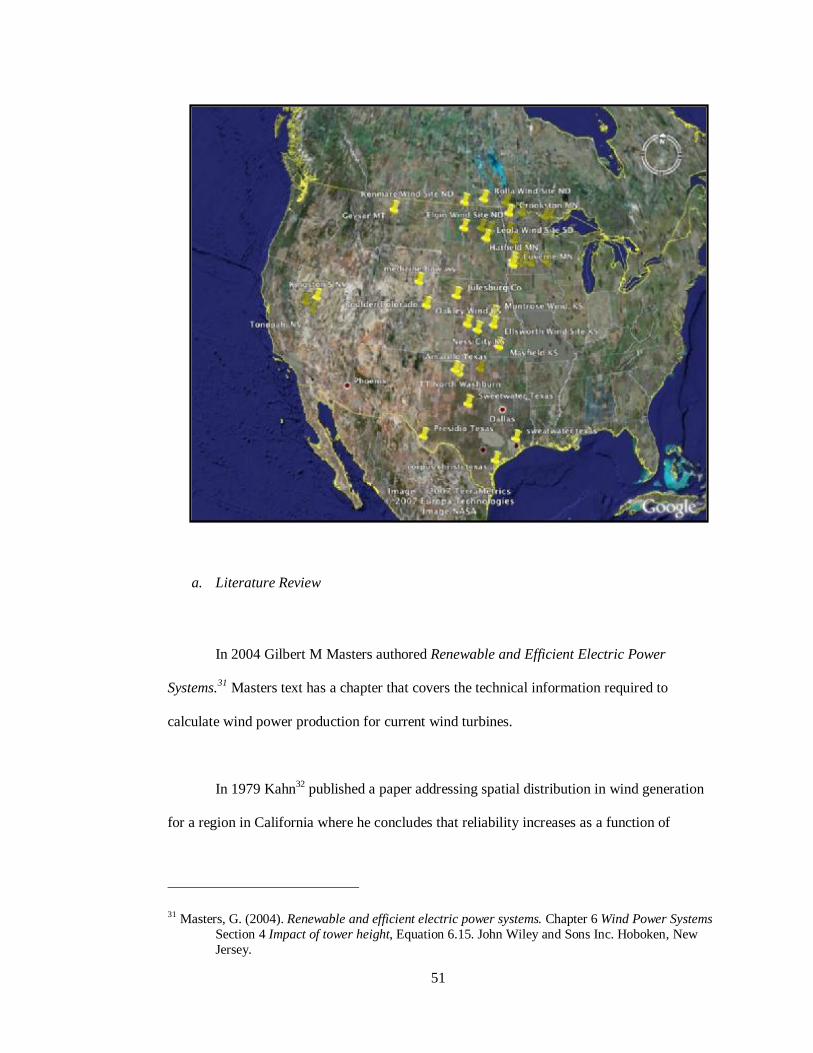
51

a. Literature Review

In 2004 Gilbert M Masters authored Renewable and Efficient Electric Power

Systems.31 Masters text has a chapter that covers the technical information required to

calculate wind power production for current wind turbines.

In 1979 Kahn32 published a paper addressing spatial distribution in wind generation

for a region in California where he concludes that reliability increases as a function of

31 Masters, G. (2004). Renewable and efficient electric power systems. Chapter 6 Wind Power Systems Section 4 Impact of tower height, Equation 6.15. John Wiley and Sons Inc. Hoboken, New Jersey.

52

geographic dispersion of wind development. Kahn also points out that integration is a

function not just the wind resources but also the rest of the system capacity.

From the late 1990’s to the current time the National Renewable Energy Laboratory

(NREL) along with co authors have published on this topic. Generally conclusions have said

increased spatial diversity decreases intermittent power outputs. 33 34

A DOE funded program titled the Plains Organization for Wind Energy Resources

(POWER) based out of the Energy and Environmental Research Center (EERC) used 28

locations between Minnesota, North Dakota, Kansas, and Iowa. This study35 used in situ data

to look at the correlation of wind speed between stations as a mean to address wind energy

production. This study concluded that: “…geographically dispersed locations reduce the

overall variability in energy production.”

Archer and Jacobson based out of Stanford University have published a series of

papers on this topic including: U.S. winds and wind power at 80 m (2003)36; Evaluation of

global wind power(2005)37; and, Supplying baseload power and reducing transmission

requirements by interconnecting wind farms (2007)38. The first two papers assess wind power

32 Kahn, Edward. (1979). The Reliability of Distributed Wind Generators. Electric Power Systems Research. Energy and Environmental Division, LBL, Berkley, CA 33 Milligan, M. Artig, R. (1999). Choosing Wind Power Plant Locations and Sizes Based on Electric Reliability Measures Using Multiple-Year Wind Speed Measurements. National Renewable Energy Laboratory Report No. CP-500-26724 34 Milligan, M. Artig, R. (1998). Reliability Benefits of Dispersed Wind Resource Development. National Renewable Energy Laboratory Report No. CP-500-24314 35 Simonson, T. Bradley, S. (DATE). Regional Wind Energy Analysis for the Central United States. Available online: www.undeerc.org/wind 36 Archer, C.L., and M.Z. Jacobson, Journal of Geophysical Research, Vol. 108, No. D9, 4289, doi:10.1029/2002JD002076, May 16, 2003 37Archer, C. M Jacobson. (2005). Evaluation of global wind power. Available online at: <http://www.stanford.edu/group/efmh/winds/aj07_jamc.pdf> 38 Archer, C.L. M.Z. Jacobson. (2007). Supplying Baseload power and reducing transmission requirements by interconnecting wind farms. Journal of Applied Meteorology and Climate.

http://www.undeerc.org/wind

http://www.stanford.edu/group/efmh/winds/aj07_jamc.pdf

53

in the US and abroad respectively these papers introduce/utilize the method of least square

extrapolation technique to obtain wind speeds at 80 M. The third paper looks at integrating

multiple wind sites to decrease intermittence in a similar fashion as what is used in this

analysis. This paper found that, “As more [wind] farms are interconnected in an array, wind

speed correlation among sites decreases and so does the probability that all sites experience

the same wind regime at the same time. Consequently, the array behaves more and more

similarly to a single farm with steady wind speed and thus steady deliverable wind power…It

was found that an average of 33% and a maximum of 47% of yearly-averaged wind power

from interconnected farms can be used as reliable, baseload electric power. Equally

significant, interconnecting multiple wind farms to a common point, then connecting that

point to a far-away city can allow the long-distance portion of transmission capacity to be

reduced, for example, by 20% with only a 1.6% loss of energy”…

A vast number of wind integration reports as well as generation assessments are

available online from private companies as well as Utilities of all sizes. These reports are

planning tools to bring wind online and deal with the challenges incurred on the electric

system. One example of those reports was produced for ERCOT in 2007.39 This report in

particular has a methods section which clearly lays out the steps for the construction of a

power production model. A power production model is a model that can take wind speeds

into the model and show power out of the model. For a review of grid integration studies a

2007 study produced by a private public working group is available.40

39 Brower, M. (2007). Electric Reliability Council of Texas: Wind Generation Assessment. AWS Truewind. Albany, New York. 40 Smith, C. Et Al. (2007). Best Practices in Grid Integration of Variable Wind Power: Summary of Recent US Case Study Results and Mitigation Measures. EWEC. Milan, Italy. Available online at: http://www.wapa.gov/UGP/PowerMarketing/WindHydro/EWEC07paper.pdf

http://www.wapa.gov/UGP/PowerMarketing/WindHydro/EWEC07paper.pdf

54

Analysis of Wind Farm Energy Produced in the United States authored by Vick,

Clark, and Carr41 looks at wind energy produced in the US between 2002 and 2006

summarizing outputs via capacity factors.

In 2005, Ms. Lena Hansen authored Can Wind Be a Firm Resource? A North

Carolina Case Study.42 This study concluded, “Geographically dispersing wind farms and

considering their output together rather than individually, significantly reduces the variability

of the wind system.” The methods from this study with regards to portfolio optimization have

been expanded and reused in the work to follow.

3.2. Methods

a. Data Collection

The first step in an analysis of wind power production is collection of wind data. Due

to the proprietary nature of wind data, attaining it is challenging. Organizations that

facilitated this data search and attainment are listed below:

1. Plains Organization for Wind Energy Resources (POWER) part of the

Energy and Environmental Research Center (EERC), based out of the

University of North Dakota. Available online at:

http://www.undeerc.org/programareas/renewableenergy/wind/default.asp

2. National Renewable Energy Laboratory (NREL). Available online at:

http://www.nrel.gov/wind/

41 Vick, B. Et Al. (2006). Analysis of Wind Farm Energy Produced in the United State. USDA- Agricultural Research Service. WTAMU-Alternative Energy Institute. 42 Hansen, L. (2005). Can wind be a firm resource? A North Carolina case study. Duke Environmental Law and Policy Forum. Vol.15:341

http://www.undeerc.org/programareas/renewableenergy/wind/default.asp

http://www.nrel.gov/wind/

55

3. Alternative Energy Institute (AEI) based out of West Texas A & M

University. Available online at: http://www.wtamu.edu/research/aei/

4. Renewable Energy Research Laboratory (RERL) based out of the Center for

Energy Efficiency and Renewable Energy (CEERE) from the University of

Massachusetts Amherst. Available online at:

http://www.ceere.org/rerl/index.html

5. The Oklahoma Wind Power Initiative (OWPI) a collaborative effort between

The University of Oklahoma and Oklahoma State University. Available

online at: http://www.seic.okstate.edu/owpi/

6. Idaho National Laboratory (INL). Available online at:

http://www.inl.gov/wind/idaho/

7. Utah Geological survey. Available online at:

http://geology.utah.gov/sep/wind/anemometerdata/sitedata.htm#data

8. Energy Resources Research Laboratory based out of Oregon State

University. Available online at: http://me.oregonstate.edu/ERRL/

9. Stanford University via Dr’s Mark Jacobson and Cristina Archer.

10. Renewable Energy Advancement in Nevada and the Southwest program

sponsored by U.S. Senator Harry Reid and is supported by NREL and in

cooperation with Desert Research Institute and Western Regional Climate

Center. Available online at: http://www.wrcc.dri.edu/nrel/

Total data acquired to this point in time totals 494 sites spread across the United States of

America. Only data sets that overlap in time can be used for this analysis. So, while nearly

500 data sites are available the greatest overlap in time yields 95 sites. Of those 95 data sets

many were not useable do to poor data quality -less then 85% good data points- or other

technical or logistical problems.

http://www.wtamu.edu/research/aei/

http://www.ceere.org/rerl/index.html

http://www.seic.okstate.edu/owpi/

http://www.inl.gov/wind/idaho/

http://geology.utah.gov/sep/wind/anemometerdata/sitedata.htm#data

http://me.oregonstate.edu/ERRL/

http://www.wrcc.dri.edu/nrel/

56

3.2.1. Data Choice

The base of literature clearly states that wind generation power output has a decrease

in intermittence with an increase in spatial diversity. But, what that decrease is has yet to be

defined. The relationship between spatial diversity and power output is a function of the

wind regime over which the system is connected. If an interconnected wind system has wind

patterns that are non-correlated the power output of the system may be less intermittent due to

the complimentary production of multiple wind farms throughout the system. In an attempt

to find the greatest diversity in wind patterns the period of time chosen for analysis

maximized: The total number of wind data sites; the total number of power pools; and the

total number of states.

Full Year Data Sets per Year

0

10

20

30

40

50

60

70

80

90

100

2004

2003

1997

2000

2005

2002

1996

1998

1999

2001

1995

2006

2007

1992

1986

1988

1991

1987

1993

1989

1990

1994

1981

1982

1983

1984

1985

1979

1980

1977

1978

1976

Year

Full Year Data Sets

Figure 3-1: Available data sets refering to distinct data recording locations per year

Figure 3-1 shows year 2004 having the greatest number of data sites available with 95

locations.

57

Diversity of Power Pools

0

1

2

3

4

5

6

YearsPower pools 4 4 5 4 4 5 5 5

1998 1999 2000 2001 2002 2003 2004 2005

Figure 3-2: Diversity of data locations by power pool

Figure 3-2 shows years 2000, 2003, and 2004 having the greatest diversity of power pools

within the data sets.

Table 3-1: Number of data sets in each of the power pools available by year

Power pools 1998 1999 2000 2001 2002 2003 2004 2005

NPCC 1 2 3 3 3 4 7 4

RFC 0 0 0 0 0 0 0 0

SERC 0 0 0 0 0 0 0 1

FRCC 0 0 0 0 0 0 0 0

ERCOT 14 8 11 7 8 9 11 11

SPP 0 0 15 0 0 2 7 0

MRO 49 50 43 42 55 51 54 40

WECC 5 3 6 3 7 24 16 21

Total sites 69 63 78 55 73 90 95 77

58

Table 3-1 breaks out the number of data sets in each power pool by year as well as the total

number of sites. The year 2004 has the greatest number of sites as well as the greatest

diversity of locations based on power pools.

Diversity of States

0

2

4

6

8

10

12

14

16

Nu

mb

er

of

Sta

tes

States 11 10 13 9 13 15 15 15

1998 1999 2000 2001 2002 2003 2004 2005

Figure 3-3: Diversity of data site locations by state

Figure 3-3 shows years 2003-2005 all having data sets from 15 states.

The year 2004 has the largest number of data sets from the largest diversity of locations.

Thus, the year 2004 was chosen for power production analysis.

3.2.2. Power Production Model

In order to assess the power output of a wind system the data sets of wind speed have

to be converted into power generation from wind turbines. This was accomplished through

the following steps:

1. Attain wind speed data

2. Import wind speed data

59

3. Align the sampling period of the data sets

4. Adjust the wind speeds to the hub height of a utility scale wind turbine

5. Adjust power curve for elevation and air density

6. Pick a wind turbine

7. Power production calculation, via a 3rd order polynomial

8. Optimization

1. Attain wind speed data

See Methods Data Collection for resources related to this topic. Attaining wind speed

data is difficult due to the proprietary nature of the data. All of the organizations and or

persons listed under Methods Data Collection were pivotal in the ability to do this analysis.

Over 1.5 years were spent searching for data sources. Working with both with University of

Colorado contacts as well as contacts from the Rocky Mountain Institute (RMI) this data set

was acquired through countless hours on the phone, Internet, and library. It is the intent of

the author, the University, and RMI to make all data that can be shared from this set available

to other researchers.

1. Import wind speed data

Once the data is located it was converted to a text file. From the text file the data was

imported into MS Excel. Depending on the format of the original data set the import function

had to be adjusted in order to capture the data in a useable format.

3. Adjust sampling period of data sets

Data was found that sampled wind speeds on a ten-minute period, a thirty-minute

period, an hourly period, a daily period, and a monthly period. This analysis was conducted

on an hourly period. All data sampled less frequently then an hourly period was not used. All

60

data sampled more frequently then an hourly period had to be converted to an hourly period.

The conversion from greater than hourly sampling, to hourly sampling, was done by taking

the hourly mean average of the more frequent samples, and reporting the average at the

beginning of each hour. This conversion was done in MS Excel with a mean average function

and a V-Look-up and reporting function. In the case that data quality information was

reported with wind speeds an average data quality figure needed to be preserved as well. Data

quality figures were preserved by taking the mode of the data quality numbers reported in the

hour data was averaged for.

3. Adjust the wind speeds to the hub height of a utility scale wind turbine

Modern utility scale wind turbines are installed with hub heights at 80 meters plus or

minus 20 meters. This analysis took all measurements made below 80 meters and scaled the

data up to 80 meters. All data collected at or above 80 meters was left as collected. The wind

speeds were adjusted for height using the one-seventh-power rule. The one-seventh-power

rule is expressed through the equation:43

(V/Vo) = (H/Ho) α

Where:

V = wind speed at height H

Vo = wind speed at height Ho

α = The friction coefficient which is a function of the terrain over which the wind is blowing

alpha in this case is assumed to be 1/7th.

43 Masters, G. (2004). Renewable and efficient electric power systems. Chapter 6 Wind Power Systems Section 4 Impact of tower height, Equation 6.15. John Wiley and Sons Inc. Hoboken, New Jersey. PG 319-321

61

To increase the validity of this analysis all attempts were made to collect data sets that were

taken at or above 80 meters.

4. Adjust power curve for elevation and air density

Due to the variety of locations data was taken from, adjustments had to be made to

the energy production ability of a turbine at any given site. This adjustment is made based on

the air density of the location from which the data was collected. Not all data sets had

temperature readings along with wind speeds so a direct calculation of air density was not

possible. Air density was estimated based on the elevation of the site. Assuming that a

turbine manufacturer can adjust the power curve of a given turbine relative to the

environmental characteristics it will be operating in. The power curve of our modeled turbine

was adjusted to the air density based on the elevation of the data collection site.

Table 3-2: Assumed air density based on elevation

Altitude above Sea Level [m] Density [kg/m3]

0.000 1.2014

152.400 1.1774

304.800 1.1533

457.200 1.1293

609.600 1.1053

762.000 1.0893

914.400 1.0732

1066.800 1.0568

1219.200 1.0404

1371.600 1.0208

1524.000 1.0012

1676.400 0.9811

1828.800 0.9611

1981.200 0.9439

2133.600 0.9267

2286.000 0.9103

2438.400 0.8938

62

2590.800 0.8778

2743.200 0.8618

2895.600 0.8458

3048.000 0.8298

Wind power production is dictated by the equation:44

Pw = 1/2CPρAV3

Where: Pw = power in watts of the wind CP= the coefficient of power, or the amount of energy extractable from the wind ρ = air density in kg/m3

A = swept area of the rotor in m2

V = wind speed

For each data location an elevation was attained and the ρ value was adjusted to account for

the air density change relative to elevation.

6. Pick a wind turbine

In order to drive out the power production equation one must chose a turbine so the

swept area as well as the operating specifications can be attained. This analysis used the

Vestas V80 2 MW wind turbine.45 One may consider pushing this set of work forward by

having a suite of turbines to choose from and depending on the average wind speeds of a

particular site picking the turbine with the cut-in, cut-out, and nominal rating wind speeds

that maximize production or value per time.

7. Power production

44 Master, G. (2004). Circular reference footnote 43. PG 325 45 Technical specifications for this turbine can be found online at: http://www.vestas.com/vestas/global/en/Products/Wind_turbines/V80_2_0.htm The use of this turbine is not an endorsement of this product

http://www.vestas.com/vestas/global/en/Products/Wind_turbines/V80_2_0.htm

63

Once all the above information is calculated the power production can be calculated

in each hour for each data set. Each hour now has an adjusted ρ, A, and V; the air density,

swept area, and the wind speed respectively.

Figure 3-4: Power curve for a V80- 2.0 MW at 1.22kg/m^2 air density

The relationship between wind speed and power output is displayed in Figure 3-4. The power

production calculation for each hour of each site is a numerical representation of the figure

shown above. Where the turbine cuts in at 3.99 ms wind speed, gains power output with the

cube of the wind speed through the 15 ms wind speed rated nominal, and the turbine cuts out

or stops production of power above 25 ms wind speed. The equation to calculate this in the

model is a 3rd order polynomial where if the wind speed is below the cut in speed no power is

produced, if the wind speed is above 25 ms no power is produced, if the wind speed is

between 15ms and 25 ms 2.0 MW of power are produced, and finally if the wind speed is

between 3.99 ms and 15 ms the power output is a function of Pw = 1/2CPρAV3.

9. Optimization

64

The following optimization methods are taken from Hansen 2005.46

The first step in determining the value of geographical dispersion is to determine

whether the sites of interest exhibit any covariance. Covariance matrices were generated for

each site relative to the other sites in their state, power pool, and the system as a whole.

Covariance matrices where driven out according to the formula:

Cov (x,y) = 1/n * Σ (xi - µx) (yi - µy)

Where: • x, y = data series • n= number of data points • µ = data point series average • i = data point

When a site exhibits negative covariance relative to another site it indicates that large

power output values at one site are associated with small power output values at another site.

This negative covariance should have the effect of reducing the variability of the combined

output of the system as a whole.

The value of this negative covariance in reducing the system variability was

determined by running an optimization model to determine the amount of capacity as a

percentage of the total generation that each site should have to yield the collective minimum

variability. This optimization problem minimizes the portfolio variability by changing the

amount of capacity development in each location, subject to several constraints, as follows:

• Minimize the covariance • Change the amount of generation at each location • Subject to: the development share at each site is greater than or equal to 0 and also

less then or equal to 1 • The total of all shares does not exceed 100% of the development

46 Hansen 2005, circular reference 42

65

• The output of the total shares is greater then or equal to a minimum specified production number

3.3. Results & Discussion

a. Data Collection

The data collection to this point has turned up 494 data collection locations. The sites

are spread out from across the USA with a concentration of data across the center swath of

the country. To facilitate further work in this area a database of all sources and specific

locations of the data is available on the Internet at:

http://www.colorado.edu/engineering/energystorage/

Graphical representation of the data sets is shown in the Methods Data Choice section.

b. Data Choice

The single year 2004 had the greatest amount of available data as well as greatest

diversity of location. Thus, 2004 is the time period chosen for analysis. Assessment of

multiple years of data in succession is of interest although the sample size of data drops

precipitously when multiple consecutive years in the same location are required. A late

development in data collection may make a multiple year BPA study possible. See Methods

Data Choice for graphical representation of what data is available.

c. Power Production Model and Optimization

The power production model calculates the energy generated in each hour of the year wind

speed data is available, for each location. An example of power production is shown for

ERCOT, Texas, five data locations.

http://www.colorado.edu/engineering/energystorage/

66

Table 3-3: Power production output for five Texas locations on a Vestas V80-2MW

Amarillo Corpus Presidio Sweetwater Washburn Date/Time kW-hr kW-hr kW-hr kW-hr kW-hr

1/1/04 0:00 698.27 570.34 77.98 179.12 478.45 1/1/04 1:00 704.73 515.19 73.11 463.16 319.08 1/1/04 2:00 677.03 447.34 55.64 1518.92 330.75 1/1/04 3:00 621.83 447.34 63.98 710.99 763.19 1/1/04 4:00 503.15 400.57 88.36 730.98 1143.08 1/1/04 5:00 294.58 415.78 225.89 807.50 1226.01 1/1/04 6:00 440.41 292.01 370.30 622.49 1283.47 1/1/04 7:00 687.60 224.92 529.48 1099.33 702.97 1/1/04 8:00 662.42 214.86 584.84 1237.17 592.19 1/1/04 9:00 602.18 130.16 429.45 796.77 354.94

1/1/04 10:00 625.81 186.46 179.00 224.66 493.72 1/1/04 11:00 602.18 195.63 0.00 0.00 541.46 1/1/04 12:00 884.44 205.09 44.55 0.00 627.72 1/1/04 13:00 1027.18 343.44 0.00 0.00 702.97 1/1/04 14:00 876.92 317.03 63.98 0.00 1116.29 1/1/04 15:00 1035.53 246.00 44.55 51.34 1170.29 1/1/04 16:00 1230.89 246.00 88.36 245.17 525.22 1/1/04 17:00 698.27 168.99 99.63 302.74 609.78 1/1/04 18:00 773.82 130.16 73.11 714.30 1013.31 1/1/04 19:00 1052.37 214.86 105.61 908.49 893.76 1/1/04 20:00 1136.32 186.46 99.63 786.13 1038.43 1/1/04 21:00 1101.06 224.92 215.93 581.13 1116.29 1/1/04 22:00 1571.41 268.35 206.26 1280.66 1531.26 1/1/04 23:00 1827.44 257.01 246.73 1464.81 2000.00

Total kWh 20,335.86 6,848.90 3,966.37 14,725.84 20,574.63 Capacity Factor 42.4% 14.3% 8.3% 30.7% 42.9%

The twenty-four hour power production output show in

Table 3-3 is represented graphically Figure 3-5.

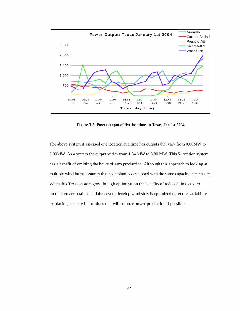
67

Power Output: Texas January 1st 2004

0

500

1,000

1,500

2,000

2,500

1/1/040:00

1/1/042:24

1/1/044:48

1/1/047:12

1/1/049:36

1/1/0412:00

1/1/0414:24

1/1/0416:48

1/1/0419:12

1/1/0421:36

Time of day (hour)

AmarilloCorpus ChristiPresidio AEISweatwaterWashburn

Figure 3-5: Power output of five locations in Texas, Jan 1st 2004

The above system if assessed one location at a time has outputs that vary from 0.00MW to

2.00MW. As a system the output varies from 1.34 MW to 5.80 MW. This 5-location system

has a benefit of omitting the hours of zero production. Although this approach to looking at

multiple wind farms assumes that each plant is developed with the same capacity at each site.

When this Texas system goes through optimization the benefits of reduced time at zero

production are retained and the cost to develop wind sites is optimized to reduce variability

by placing capacity in locations that will balance power production if possible.

68

Mean Variance Frontier

0

50,000

100,000

150,000

200,000

250,000

300,000

350,000

300 350 400 450 500 550Minimum Average Power Production (kW)

Mean Variance Frontier

Figure 3-6: Texas system mean variance frontier

Figure 3-6 shows increasing portfolio variability with increasing minimum average

power production. The goal of this work is to minimize intermittent power production thus

decreasing the portfolio variability. The variability in the Texas system shown above

increases minimally through the minimum output of 400kW where variability begins to

increase at a steeper slope and at 500kW the variability becomes vertical. Developing this

system with the intent of the highest minimum average power production with the lowest

portfolio variability one specify optimization at 400 kW minimum average power production.

Out of a 2MW machine 400kW is 20% firm. When the model runs this optimization the

development is specified at:

• Amarillo = 0% • Corpus Christi = 51% • Presidio =0% • Sweetwater = 9% • Washburn = 40%

69

Power Output: Texas January 1st 2004

0

200

400

600

800

1,000

1,200

1,400

1,600

1,800

2,000

1/1/04 0:00 1/1/04 2:24 1/1/04 4:48 1/1/04 7:12 1/1/04 9:36 1/1/04 12:00 1/1/04 14:24 1/1/04 16:48 1/1/04 19:12 1/1/04 21:36

Time of day (hour)

AmarilloCorpus ChristiPresidio AEISweatwaterWashburnOptimized Wind Array

Figure 3-7: Optimized output of the Texas system on Jan 1st 2004

Figure 3-7 shows the output of the Texas system with the intent to minimize intermittence

while maximizing output. This optimization is not the highest energy output possible, but it is

the highest energy output attainable with a specified 20% firm power. The previous series of

charts displayed one day out of 365 days of analysis. The full year of the Texas system is

shown in a histogram format in Figure 3-8.

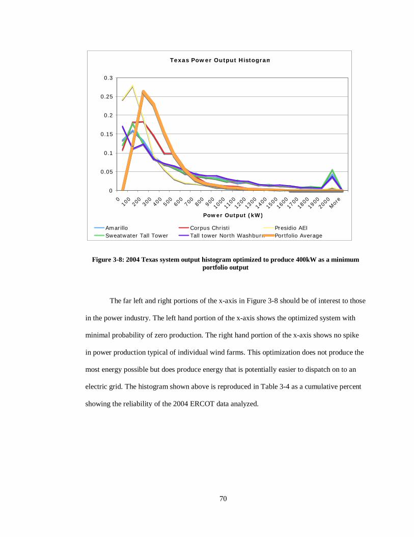
70

Texas Power Output Histogram

0

0.05

0.1

0.15

0.2

0.25

0.3

010

020

030

040

050

060

070

080

090

010

0011

0012

0013

0014

0015

0016

0017

0018

0019

0020

00Mor

e

Power Output (kW)

Amarillo Corpus Christi Presidio AEISweatwater Tall Tower Tall tower North Washburn Portfolio Average

Figure 3-8: 2004 Texas system output histogram optimized to produce 400kW as a minimum portfolio output

The far left and right portions of the x-axis in Figure 3-8 should be of interest to those

in the power industry. The left hand portion of the x-axis shows the optimized system with

minimal probability of zero production. The right hand portion of the x-axis shows no spike

in power production typical of individual wind farms. This optimization does not produce the

most energy possible but does produce energy that is potentially easier to dispatch on to an

electric grid. The histogram shown above is reproduced in Table 3-4 as a cumulative percent

showing the reliability of the 2004 ERCOT data analyzed.

71

Table 3-4: System reliability percentage at x percent of capacity

System Reliability % Capacity % Optimized

System Amarillo Corpus Presidio Sweetwater Washburn

0% 0.03% 13.46% 10.82% 24.24% 12.14% 17.10% 5% 99.97% 86.54% 89.18% 75.76% 87.86% 82.90%

10% 87.77% 70.51% 71.02% 47.77% 69.98% 71.78%

15% 61.51% 57.30% 52.65% 28.54% 57.64% 59.43% 20% 38.64% 48.20% 38.08% 19.11% 49.17% 51.04% 25% 23.30% 41.29% 28.21% 13.43% 42.08% 43.82% 30% 13.87% 34.88% 18.33% 10.27% 36.11% 37.33% 35% 8.39% 30.43% 12.50% 8.20% 31.48% 31.96% 40% 5.58% 25.88% 8.82% 6.38% 27.53% 27.55% 45% 3.84% 22.50% 6.73% 4.96% 24.02% 23.57% 50% 2.49% 19.00% 5.25% 4.22% 20.87% 19.58% 55% 1.68% 16.36% 4.05% 3.44% 18.42% 16.51% 60% 1.02% 14.30% 3.02% 2.89% 15.79% 14.00% 65% 0.68% 12.02% 2.50% 2.48% 13.68% 11.60% 70% 0.46% 10.39% 1.94% 1.97% 12.19% 10.02% 75% 0.23% 9.01% 1.57% 1.70% 10.60% 8.63% 80% 0.10% 7.72% 1.30% 1.54% 9.37% 7.14% 85% 0.07% 6.71% 1.18% 1.26% 8.19% 5.94% 90% 0.01% 5.84% 0.99% 1.06% 7.40% 5.15% 95% 0.00% 5.04% 0.83% 0.97% 6.27% 4.34% 100% 0.00% 4.41% 0.72% 0.84% 5.53% 3.61%

Table 3-4 shows the numerical result of the histogram above. The optimized system

significantly reduces both the time spent at zero production as well as the power spike

traditionally found at 100% production or speeds over nominal. The 3% probability of zero

production in the optimized system results in the equivalent of 11 days of zero production per

year where as each of the systems individually would have the following days of zero

production:

• Amarillo- 49 days of zero production • Corpus- 40 days of zero production • Presidio- 89 days of zero production • Sweetwater- 44 days of zero production • Washburn- 62 days of zero production

72

Each of the other systems analyzed had results with trends similar to that of the Texas

system.

MN Power Output Histogram

0.00

0.05

0.10

0.15

0.20

0.25

0.30

0.35

0.40

0 100 200 300 400 500 600 700 800 900 1000 1100 1200 1300 1400 1500 1600 1700 1800 1900 2000

Power Output (kW)

Alberta Wind Monitoring Site Breckenridge Wind Monitoring Site Brewster Wind Monitoring Site

Crookston Wind Monitoring Site Fountain Wind Monitoring Site Hallock Wind Monitoring Site

Hatfield Wind Monitoring Site Hector Wind Monitoring Site Hoyt Lakes Wind Monitoring Site

Isabella Wind Monitoring Site Lucan Wind Monitoring Site Luverne Wind Monitoring Site

Marshall Wind Monitoring Site Mountain Lake Wind Monitoring Site Red Lake Wind Monitoring Site

Rochester Wind Monitoring Site St. Killian Wind Monitoring Site Winnebago Wind Monitoring Site

Optimized MN Wind

Figure 3-9: 2004 optimized Minnesota wind system

Table 3-5: Minnesota 2004 reliability percent as a percentage of total capacity when optimized

Capacity % Optimized MN Wind System 0 0.91% 5 99.09% 10 72.77% 15 56.53% 20 44.42% 25 35.19% 30 28.34% 35 23.09% 40 19.23% 45 15.86% 50 13.05% 55 10.85% 60 8.75% 65 7.29% 70 5.91% 75 4.79% 80 3.72% 85 2.89%

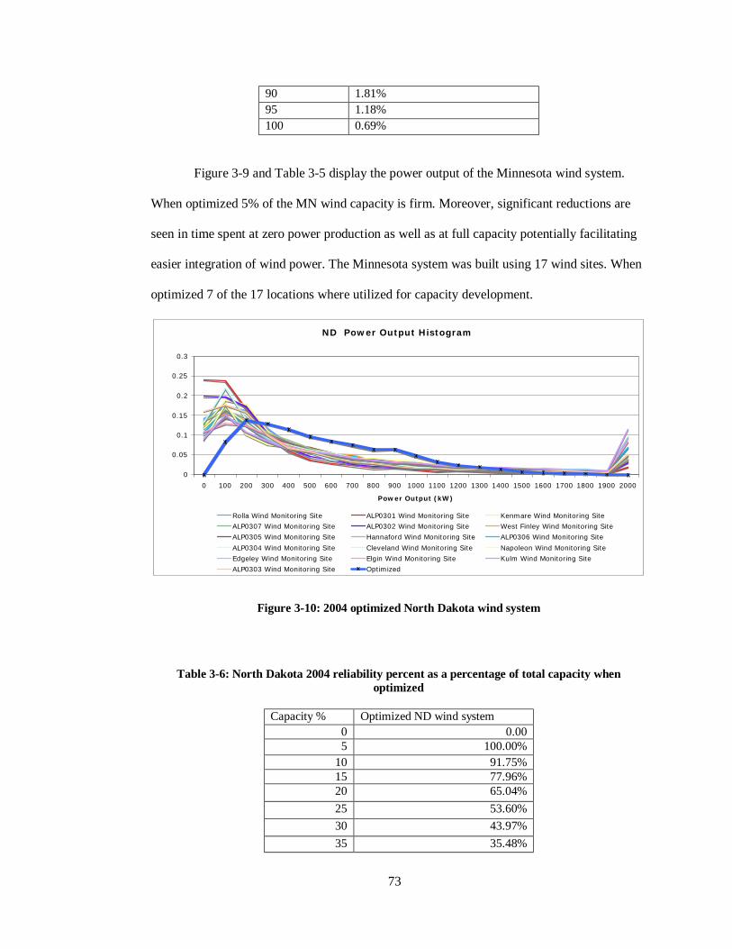
73

90 1.81% 95 1.18% 100 0.69%

Figure 3-9 and Table 3-5 display the power output of the Minnesota wind system.

When optimized 5% of the MN wind capacity is firm. Moreover, significant reductions are

seen in time spent at zero power production as well as at full capacity potentially facilitating

easier integration of wind power. The Minnesota system was built using 17 wind sites. When

optimized 7 of the 17 locations where utilized for capacity development.

ND Power Output Histogram

0

0.05

0.1

0.15

0.2

0.25

0.3

0 100 200 300 400 500 600 700 800 900 1000 1100 1200 1300 1400 1500 1600 1700 1800 1900 2000

Power Output (kW)

Rolla Wind Monitoring Site ALP0301 Wind Monitoring Site Kenmare Wind Monitoring Site

ALP0307 Wind Monitoring Site ALP0302 Wind Monitoring Site West Finley Wind Monitoring Site

ALP0305 Wind Monitoring Site Hannaford Wind Monitoring Site ALP0306 Wind Monitoring Site

ALP0304 Wind Monitoring Site Cleveland Wind Monitoring Site Napoleon Wind Monitoring Site

Edgeley Wind Monitoring Site Elgin Wind Monitoring Site Kulm Wind Monitoring Site

ALP0303 Wind Monitoring Site Optimized

Figure 3-10: 2004 optimized North Dakota wind system

Table 3-6: North Dakota 2004 reliability percent as a percentage of total capacity when optimized

Capacity % Optimized ND wind system 0 0.00 5 100.00%

10 91.75% 15 77.96% 20 65.04% 25 53.60% 30 43.97% 35 35.48%

74

40 27.97% 45 21.64% 50 15.24% 55 10.52% 60 7.31% 65 4.95% 70 3.05% 75 1.79% 80 1.16% 85 0.66% 90 0.30% 95 0.03%

100 0.01%

Figure 3-10 and Table 3-6 display the power output of the North Dakota wind

system. When optimized 5% of the wind capacity is firm. Moreover, significant reductions

are seen in time spent at zero power production as well as at full capacity potentially

facilitating easier integration of wind power. The North Dakota system was built using 16

wind sites. When optimized 10 of the 16 locations where utilized for capacity development.

75

MRO Power Output Histogram

0

0.05

0.1

0.15

0.2

0.25

0.3

0.35

0.4

0.45

010

020

030

040

050

060

070

080

090

010

0011

0012

0013

0014

0015

0016

0017

0018

0019

0020

00

Power Output (kW)

Rolla Wind Monitoring Site ALP0301 Wind Monitoring Site Kenmare Wind Monitoring Site ALP0307 Wind Monitoring Site

ALP0302 Wind Monitoring Site West Finley Wind Monitoring Site ALP0305 Wind Monitoring Site Hannaford Wind Monitoring Site

ALP0306 Wind Monitoring Site ALP0304 Wind Monitoring Site Cleveland Wind Monitoring Site Napoleon Wind Monitoring Site

Edgeley Wind Monitoring Site Elgin Wind Monitoring Site Kulm Wind Monitoring Site ALP0303 Wind Monitoring Site

Optimized ND Alberta Wind Monitoring Site Breckenridge Wind Monitoring Site Brewster Wind Monitoring Site

Crookston Wind Monitoring Site Fountain Wind Monitoring Site Hallock Wind Monitoring Site Hatfield Wind Monitoring Site

Hector Wind Monitoring Site Hoyt Lakes Wind Monitoring Site Isabella Wind Monitoring Site Lucan Wind Monitoring Site

Luverne Wind Monitoring Site Marshall Wind Monitoring Site Mountain Lake Wind Monitoring Site Red Lake Wind Monitoring Site

Rochester Wind Monitoring Site St. Killian Wind Monitoring Site Winnebago Wind Monitoring Site Optimized MN Wind

% Optimized MRO

Figure 3-11: 2004 optimized MRO wind system, which includes both Minnesota and North Dakota

Table 3-7: Midwest reliability organization 2004 reliability percent as a percentage of total capacity when optimized

Capacity % Optimized MRO wind system 0 0.07% 5 99.93%

10 91.30% 15 76.50% 20 62.06% 25 48.62% 30 39.26% 35 32.05% 40 26.29% 45 20.93% 50 16.04% 55 11.98% 60 9.08% 65 6.64% 70 4.11%

76

75 2.41% 80 1.22% 85 0.72% 90 0.35% 95 0.02% 100 0.00%

Figure 3-11 and Table 3-7 display the power output of the MRO wind system. When

optimized 5% of the MRO system wind capacity is firm. Moreover, significant reductions are


easier integration of wind power. The MRO system was built using 35 wind sites. When


Kansas Power Output Histogram

0

0.02

0.04

0.06

0.08

0.1

0.12

0.14

0.16

0.18

0.2

010

020

030

040

050

060

070

080

090

010

0011

0012

0013

0014

0015

0016

0017

0018

0019

0020

00

Power Output (kW)

Ellsworth Wind Monitoring Site Mayfield Wind Monitoring Site Montrose Wind Monitoring SiteNess City Wind Monitoring Site Oakley Wind Monitoring Site Ulysses Wind Monitoring SiteOptimized System

Figure 3-12: 2004 optimized Kansas wind system

Table 3-8: Kansas 2004 reliability percent as a percentage of total capacity when optimized

Capacity % Optimized KS wind system 0 0.41% 5 99.59%

77

10 84.93% 15 71.51% 20 60.43% 25 51.24% 30 43.70% 35 37.82% 40 33.20% 45 28.92% 50 25.43% 55 22.52% 60 19.60% 65 17.02% 70 14.88% 75 12.31% 80 10.13% 85 7.65% 90 5.23% 95 3.16% 100 1.15%

Figure 3-12 and Table 3-8 display the power output of the Kansas wind system.

When optimized 5% of the KS wind capacity is firm. Moreover, significant reductions are


easier integration of wind power. The Kansas system was built using 6 wind sites. When


3.4. Conclusions and Next Steps

To improve the quality of this assessment a number of steps can be taken. The quality

of data can be improved by having data taken from hub height as opposed to ramping up

wind speeds. There is a cost to collecting wind speed data but surely it is less costly to have

multiple tall tower anemometer programs then it is to build a wind system that is less then

optimal. While developers do take hub height data, they do this in specific location that they

would like to develop. Data is not taken in multiple locations with the intent to optimize. As a

youngster we learn think before you speak, to those in the wind industry one might suggest

think and optimize before you build.

78

Turbine choice can be optimized for each location to maximize the production from

each wind farm prior to optimizing the system as a whole. Wind speed data can be taken from

functioning wind farms or significant wind resource areas. Many of the wind speed data

locations used in this analysis where less then optimal. This analysis showed wind power can

be firm at a low percentage of its total capacity when it is optimized. If the best wind

locations with quality data attempted to optimize larger benefits may be found. Finally this

optimization was conducted using Solver in MS Excel; while this tool is a good start to

optimization stronger optimization methods should be used.

As an analogy to the challenges with this analysis; if one takes Lincoln logs and

builds a geodesic structure to assess its structural soundness they would see a relatively

strong Lincoln log structure. Although, that Lincoln log based improvement would be small

due to the toy like nature of the Lincoln log. If one took viable building material and built a

geodesic dome they would find significant structural improvements. The data used in this

analysis can be seen as the Lincoln log version of wind speed data. Wind power developers,

Public Utility Commissions, and others should facilitate the availability of quality data to

truly assess potential improvements in the ability to firm wind power. That firming would be

done first through optimization of spatial diversity and then other steps. Today wind

developers see their wind data as a proprietary resource that should be kept private to ensure

financial solvency. If sharing data would allow optimization of the wind system it would

bring a higher value to the power purchase agreement (PPA) of those companies. Financial

solvency maybe facilitated by sharing information as opposed to keeping it private.

This analysis shows wind is a firm resource when optimized at 5% of the total

capacity developed. A larger percentage of wind power may be considered firm through

improvement in data resources, optimization methods, or equipment utilization. Additionally

looking beyond wind generation optimization firming may be achieved through other

renewable resources, energy storage, demand response, and efficiency. All of the steps

79

mentioned will surely yield a significantly firmer renewable resource then utility companies

are dealing with today.

4. A spatially optimized and PHES integrated wind energy system

The firming benefits garnered from optimizing spatial distribution of wind capacity

combined with the firming benefits of energy storage are two significant steps towards

firming the energy output of a wind system. Keeping in mind that many other firming steps

can be taken including; demand response, dispatchability of loads, efficiency of loads, power

wheeling, and additional clean generation sources (to name a few other partial solutions)

looking at spatial diversity and energy storage in tandem is a strong step forward.

Using the power output from five Texas wind plants for the year 2004 the following

series of charts explores the benefits of combining optimized spatial distribution with PHES.

This modeling stores and deploys wind energy without putting additional energy into the

system from other generating sources. Due to the fact that no additional energy is put into the

energy generation and storage system shown here it is impossible to have reliable power

beyond the capacity factor of the wind energy system multiplied with the efficiency of the

storage mechanism. Although the following analysis starts to look at these mitigation

techniques combined, the modeling to yield these results is flawed. This modeling is flawed

because there is not a limit on the amount of energy that can be stored. Meaning this

calculation assumes an unlimited reservoir size. Additionally this model dispatches energy to

minimize power output variability not to maximize economic value or to match load

characteristics. Bringing in the above mentioned factors would be a strong addition to this

work.

The following figures will show wind energy output without spatial distribution,

followed by wind energy with spatial distribution, followed by wind energy with spatial

distribution and increasing amounts of PHES capacity relative to the wind capacity. Where

80

the term “% of Capacity” is used, it means the power output as a percent of the rated capacity

of the installed generation.

Sweetwater 2004 power output

0%10%20%30%40%50%60%70%80%90%

100%

1/1/

2004

2/1/

2004

3/1/

2004

4/1/

2004

5/1/

2004

6/1/

2004

7/1/

2004

8/1/

2004

9/1/

2004

10/1

/200

4

11/1

/200

4

12/1

/200

4

Time

% o

f Cap

acity

. Sweetwater 2004 power output

Figure 4-1: Sweetwater Texas 2004 power output

Figure 4-1 displays the power output of a wind farm as a percent of rated capacity in

the year 2004. This output is from a single wind location with no energy storage. This single

location, no storage, example of wind energy production displays the greatest amount of

variability of any of the examples in this section. Wind energy produced in the year 2007 is

seen by system operator on electric grid much like the output shown in Figure 4-1 and then

backed up with fast responding generation.

81

Texas 2004 optimized system power output

0%10%20%30%40%50%60%70%80%90%

100%

1/1/

2004

2/1/

2004

3/1/

2004

4/1/

2004

5/1/

2004

6/1/

2004

7/1/

2004

8/1/

2004

9/1/

2004

10/1

/200

4

11/1

/200

4

12/1

/200

4

Time

% o

f Cap

acity

.

Texas optimized system

Figure 4-2: Texas wind system optimized to decrease variability utilizing spatial distribution

Figure 4-2 relative to Figure 4-1 displays significant improvement in ability to

decrease variability. Figure 3-8 displays this output in a histogram format. The above output

simply optimizes the spatial diversity of wind capacity development and significantly

decreases time at 0% output and shows reliability of 5% capacity over 99% of the year.

Texas optimized system plus 10% storage capacity

0%10%20%30%40%50%60%70%80%90%

100%

1/1/

2004

2/1/

2004

3/1/

2004

4/1/

2004

5/1/

2004

6/1/

2004

7/1/

2004

8/1/

2004

9/1/

2004

10/1

/200

4

11/1

/200

4

12/1

/200

4

Time

% o

f Cap

acity

. Texas optimized system plus

10% storage capacity

Figure 4-3: Texas wind system optimized to decrease variability utilizing spatial distribution and 10% capacity of PHES

Figure 4-3 displays the Texas optimized system with 10% of capacity backed up with

PHES. This sizing of storage creates 100% reliability at 10% of capacity. At the end of the

82

modeled year (2004) the storage reservoir had significant reserves of stored energy that were

not deployed. Non-deployment would not happen in reality due to limited storage size, as

well as the value of deployment and other factors. Never the less, with 10% of wind capacity

backed up with storage, 10% of capacity becomes reliable 100% of the year.


0%10%20%30%40%50%60%70%80%90%

100%

1/1/

2004

2/1/

2004

3/1/

2004

4/1/

2004

5/1/

2004

6/1/

2004

7/1/

2004

8/1/

2004

9/1/

2004

10/1

/200

4

11/1

/200

4

12/1

/200

4

Time

% o

f Cap

acity




Figure 4-4 displays the 2004 Texas optimized wind system with 20% of rated

capacity backed up with PHES. This spatial optimization along with storage yields 20% of

capacity reliable 87% of the year. Spatial optimization without PHES backup resulted in 20%

of capacity reliable 39% of the year. Adding storage to the optimization yields an

improvement in reliability at 20% capacity, of 48%. This sizing of storage is the same value

as the mean average power output of the Texas optimized system. Aligning the mean average

output of the optimized system and the capacity of the storage development tends to result in

both a high reliability at the specified capacity, and a small amount of energy retained in the

storage reservoir at the end of the modeled period. Aligning storage with the mean average

output results in nicely sized development because sizing for the mean average allows the

times of low generation to be compensated by the times of high generation (less the

83

efficiency loss of the system). When looking at a real interconnected system as opposed to

this modeled system one would see less variability because additional power generation

would be added into the system when economically prudent.


0%10%20%30%40%50%60%70%80%90%

100%1/

1/20

04

2/1/

2004

3/1/

2004

4/1/

2004

5/1/

2004

6/1/

2004

7/1/

2004

8/1/

2004

9/1/

2004

10/1

/200

4

11/1

/200

4

12/1

/200

4

Time

% o

f Cap

acity




Figure 4-5 displays the optimized 2004 Texas wind system with 30% of capacity

backed up with PHES. This output show a significant amount of time where this energy

system is not able to deploy, or is not reliable. Note that no energy is allowed to be used in

this system that was not generated by the wind system analyzed. Thus, as the capacity of

PHES reaches the capacity factor of the wind system multiplied by the efficiency loss of the

storage without additional energy inputs, firming the output is not possible.

Although only two methods of integration are discussed above, the most effective

solution to generation variability will be an integrated approach, which should include:

1. Diversifying the types and locations of renewable generation sources. This method

should be an optimization of spatial diversity and renewable generation source that

minimizes intermittence and cost while maximizing capacity to meet or exceed RPS

targets while meeting loads.

84

2. Encouraging demand side management (DSM) to serve as a renewable source of

energy as well as enabling the dispatchability of loads.

3. Developing adequate transmission infrastructure to facilitate diversified renewable

plant locations. As well as imbedding intelligence into this system improving

communications and management of resources on the grid.

4. Planning for additional energy storage on the electric grid that optimizes the

utilization of transmission and generation resources minimizing costs and GHG

emissions, allowing renewable energy to be dispatchable.

5. Formulate legislation that provides incentives for the first four points, smoothing

intermittent generation as well as planning for storage to compensate times of excess

and shortage.

None of the above points are silver bullets to facilitate 20% and greater penetration of

renewable power sources. Moreover, if only one of the above strategies is pursued it will be

less valuable than if a combination are pursued. Each point will increase the reliability of the

electric grid and have synergistically positive effects on the other points.

85

86

Bibliography

Archer, C. Jacobson, M. 2003. Spatial and temporal distributions of U.S. winds and wind

power at 80 m derived from measurements. Journal of Geophysical Research. Vol. 108, No.

D9, 4289, doi:10.1029/2002JD002076

Archer, C. Jacobson, M. 2005. Evaluation of global wind power. Available online at:


Archer, C. Jacobson, M. 2007. Supplying Baseload power and reducing transmission

requirements by interconnecting wind farms. Journal of Applied Meteorology and Climate.

Armstrong E. Mermel T. 1974. Converting Existing Hydro-Electric Dams and Reservoirs

into Pumped Storage Facilities. American Society of Civil Engineers. New York, NY.

Benitez, P. Dragulescu, L. and Van Kooten, C. 2006. The Economics of Wind Power with

Energy Storage. Resource and Environmental Economics and Policy Analysis (REPA)

Research Group. pp. 1-38, 2006.

Brower, M. 2007. Electric Reliability Council of Texas: Wind Generation Assessment. AWS

Truewind. Albany, New York.


87

Buena C. Carta J. October 2006. Wind powered pumped hydro storage systems, a means of

increasing the penetration of renewable energy in the Canary Islands. Renewable and

Sustainable Energy Reviews. 312-340

Chiu, L Et Al. 1978. Mechanical Energy Storage Systems: Compressed Air and Underground

Pumped Hydro. AIAA. Huntsville Alabama.

Hansen, L. 2005. Can wind be a firm resource? A North Carolina case study. Duke

Environmental Law and Policy Forum. Vol.15:341

Harpman D. 2006. Exploring the Economic Value of Hydropower in the Interconnected

electricity System. Available online at: http://mysite.du.edu/~dharpman/profdownload.html.

Also available from NTIS

Hight, H W. Jan 1971. Cabin Creek Pumped Storage Hydroelectric Project. Journal of the

Power Division. Proceedings of the American Society of Civil Engineers.

Irving, D. Haines, B. Modde, T. (2003). White River Base Flow Study, Colorado and Utah,

1995-1996. Upper Colorado River Basin Recovery Implementation Program.

Kahn, Edward. 1979. The Reliability of Distributed Wind Generators. Electric Power

Systems Research. Energy and Environmental Division, LBL, Berkley, CA


88

Lawrence, P. Cornelis, G. Van Kooten. Murray Love. and Ned Djilali. 2005. Utility-Scale

Wind Power: Impacts of Increased Penetration. Paper No. IGEC-097. Proceedings of the

International Green Energy Conference. Waterloo, Ontario, Canada.

Lawrence, S.2006. Hydro Power Lecture. Lecture noteSYST6820(2006). Available online at:

leeds-faculty.colorado.edu/lawrence/syst6820/Lectures/Hydropower.ppt

Levine & Barnes. 2007. Potential Pumped Hydroelectric Energy Storage Sites in Colorado.

EESAT Conference Proceedings Paper. Available online at:

http://www.colorado.edu/engineering/energystorage/files/EESAT2007/EESAT_Colorado_P

HES_Sites_Paper.pdf

Liu, Jia, G. Cornelis van Kooten and Lawrence Pitt. June 2005. Integrating Wind Power in

Electricity Grids: An Economic Analysis. Paper No. IGEC-1-017 in Proceedings of the

International Green Energy Conference. Waterloo, Ontario, Canada. Available:


Masters, G. 2004. Renewable and efficient electric power systems. Chapter 6 Wind Power

Systems Section 4 Impact of tower height, Equation 6.15. John Wiley and Sons Inc. Hoboken,

New Jersey.

Milligan, M. Artig, R. 1999. Choosing Wind Power Plant Locations and Sizes Based on

Electric Reliability Measures Using Multiple-Year Wind Speed Measurements. National

Renewable Energy Laboratory Report No. CP-500-26724

http://www.colorado.edu/engineering/energystorage/files/EESAT2007/EESAT_Colorado_P


89

Milligan, M. Artig, R. 1998. Reliability Benefits of Dispersed Wind Resource Development.

National Renewable Energy Laboratory Report No. CP-500-24314

Oakleaf, B. Nov 29, 2006. RMEL Renewables Conference: New Developments in

Applications. Denver Colorado. Available online at: http://www.rmel.org

Simonson, T. Bradley, S. (DATE). Regional Wind Energy Analysis for the Central United

States. Available online: www.undeerc.org/wind

Smith, C. Et Al. 2007. Best Practices in Grid Integration of Variable Wind Power: Summary

of Recent US Case Study Results and Mitigation Measures. EWEC. Milan, Italy. Available

online at: http://www.wapa.gov/UGP/PowerMarketing/WindHydro/EWEC07paper.pdf

Stone & Webster Management Consultants. 1988. Colorado Joint Planning Study

Economic Potential of Pumped Storage. Colorado, Denver

Tester, J. W. 2005. Sustainable Energy Choosing among Options, I ed., vol. 1, S. Howe, Ed.

Cambridge, Massachusetts: The MIT Press, 2005

US Department of the Interior Bureau of Reclamation. 1984. Wind Hydroelectric Energy

Project Wyoming: Status Report on System Verification Units.

US Department of the Interior Bureau of Reclamation. April 1978. Potential Power Additions

To The Colorado-Big Thompson Project Pick-Sloan Missouri Basin Program Colorado

http://www.rmel.org

http://www.undeerc.org/wind

http://www.wapa.gov/UGP/PowerMarketing/WindHydro/EWEC07paper.pdf

90

US Department of the Interior Bureau of Reclamation. Mount Elbert Pumped Storage Power

Plant. Available online at: http://www.usbr.gov/power/data/sites/mtelbert/mtelbert.html

US Department of the Interior Bureau of Reclamation. Colorado-Big Thompson Project

Engineering Data. Available online at: http://www.usbr.gov/dataweb/html/gpcbtengdata.html

US Department of the Interior Bureau of Reclamation. April 1978. Potential Power Additions

To The Colorado-Big Thompson Project Pick-Sloan Missouri Basin Program Colorado

Vick, B. Et Al. 2006. Analysis of Wind Farm Energy Produced in the United State. USDA-

Agricultural Research Service. WTAMU-Alternative Energy Institute.

Wood A. Wollenberg B. 1996. Power Generation, Operation, and Control. Wiley-

Interscience Publication, John Wiley and Sons, Inc. New York NY.


http://www.usbr.gov/dataweb/html/gpcbtengdata.html

91

Glossary of Terms

Base Load- The minimum load over a given period of time, typically slow responding to

changes in need. This resource generally has the lowest cost of energy in a traditional

assessment.

Capacity- The maximum load that a machine, station, or system can carry under existing

service conditions. Equivalent term: peak capability, peak generation, firm peak load,

carrying capability. In transmission, the maximum load a transmission line is capable of

carrying.

Capacity Factor- Capacity factor is connected with a power generator and is defined as the

factor determined by dividing the energy delivered by generator during a given period by the

energy that would have been delivered if the generator had been delivering energy at its

maximum capacity every hour in that time period.

Energy- The capacity for performing work. The electrical energy term generally is kWh and

represents power (kW) operation for some time period (h).

Energy, Electric- It is measured in terms of the work it is capable of doing; electric energy is

usually measured in kWh. The heat equivalent of one kWh is equal to 3,412.97 Btu’s.

Energy, Off-Peak, Electricity- Energy supplied during period of relatively low system

demands.

Energy, On-Peak, Electricity- Energy supplied during periods of relatively high system

demands.

92

Head – The effective head is the upper elevation of a hydro site minus the lower elevation

and yield the H or effective head of a site, this is expressed in meters (m).

Load- The amount of electric power or energy delivered or required at any specified point or

points on a system. Load originates primarily at the energy consuming equipment of the

customers.

Load Curve- A curve of power versus time sowing the value of a specific load for each unit

of the period covered.

Loss of Load Probability (LOLP)- A measure of the probability that a system demand will

exceed capacity during a given period, often expressed as the expected number of days per

year over a long period, frequently taken as 10 consecutive years. An example of LOLP is

one day in 10 years.

Pumped Storage- An arrangement whereby a reservoir is filled with water by pumping

during off-pear periods when low cost energy is available or when water is being spilled at

other hydro plants. This method of operating hydro plants stores water which can be used to

meet peak loads.

Pumped Storage Plant (PHES)- A hydroelectric power plant, which generates electric

energy on demand. Many times these plants function for peak-load use by utilizing water

pumped into a storage reservoir during off-peak periods.

93

Renewable Penetration Percent, Penetration %- Total capacity of renewable generation/

Total system Capacity.

Spinning Reserve- Generating units operation at a no load or at partial load with excess

capacity readily available to support additional load.