Embed Size (px)
Citation preview
3Pulse Propagation in Dispersive Media
In this chapter, we examine some aspects of pulse propagation in dispersive media andthe role played by various wave velocity definitions, such as phase, group, and front ve-locities. We discuss group velocity dispersion, pulse spreading, chirping, and dispersioncompensation, and look at some slow, fast, and negative group velocity examples. Wealso present a short introduction to chirp radar and pulse compression, elaborating onthe similarities to dispersion compensation. The similarities to Fresnel diffraction andFourier optics are discussed in Sec. 20.1. The chapter ends with a guide to the literatureon these diverse topics.
3.1 Propagation Filter
As we saw in the previous chapter, a monochromatic plane wave moving forward alongthe z-direction has an electric field E(z)= E(0)e−jkz, where E(z) stands for either the xor the y component. We assume a homogeneous isotropic non-magnetic medium (μ =μ0) with an effective permittivity ε(ω); therefore, k is the frequency-dependent andpossibly complex-valued wavenumber defined by k(ω)= ω
√ε(ω)μ0. To emphasize
the dependence on the frequency ω, we rewrite the propagated field as:†
E(z,ω)= e−jkzE(0,ω) (3.1.1)
Its complete space-time dependence will be:
ejωtE(z,ω)= ej(ωt−kz)E(0,ω) (3.1.2)
A wave packet or pulse can be made up by adding different frequency components,that is, by the inverse Fourier transform:
E(z, t)= 1
2π
∫∞−∞ej(ωt−kz)E(0,ω)dω (3.1.3)
†where the hat denotes Fourier transformation.
84 3. Pulse Propagation in Dispersive Media
Setting z = 0, we recognize E(0,ω) to be the Fourier transform of the initial wave-form E(0, t), that is,
E(0, t)= 1
2π
∫∞−∞ejωtE(0,ω)dω � E(0,ω)=
∫∞−∞e−jωtE(0, t)dt (3.1.4)
The multiplicative form of Eq. (3.1.1) allows us to think of the propagated field asthe output of a linear system, the propagation filter, whose frequency response is
H(z,ω)= e−jk(ω)z (3.1.5)
Indeed, for a linear time-invariant system with impulse response h(t) and corre-sponding frequency response H(ω), the input/output relationship can be expressedmultiplicatively in the frequency domain or convolutionally in the time domain:
Eout(ω)= H(ω)Ein(ω)
Eout(t)=∫∞−∞h(t − t′)Ein(t′)dt′
For the propagator frequency response H(z,ω)= e−jk(ω)z, we obtain the corre-sponding impulse response:
h(z, t)= 1
2π
∫∞−∞ejωtH(z,ω)dω = 1
2π
∫∞−∞ej(ωt−kz)dω (3.1.6)
Alternatively, Eq. (3.1.6) follows from (3.1.3) by setting E(0,ω)= 1, correspondingto an impulsive input E(0, t)= δ(t). Thus, Eq. (3.1.3) may be expressed in the timedomain in the convolutional form:
E(z, t)=∫∞−∞h(z, t − t′)E(0, t′)dt′ (3.1.7)
Example 3.1.1: For propagation in a dispersionless medium with frequency-independent per-mittivity, such as the vacuum, we have k =ω/c, where c = 1/√με. Therefore,
H(z,ω)= e−jk(ω)z = e−jωz/c = pure delay by z/c
h(z, t)= 1
2π
∫ ∞−∞ej(ωt−kz)dω = 1
2π
∫∞−∞ejω(t−z/c)dω = δ(t − z/c)
and Eq. (3.1.7) gives E(z, t)= E(0, t − z/c), in agreement with the results of Sec. 2.1. ��
The reality of h(z, t) implies the hermitian property,H(z,−ω)∗= H(z,ω), for thefrequency response, which is equivalent to the anti-hermitian property for the wave-number, k(−ω)∗= −k(ω).
3.2. Front Velocity and Causality 85
3.2 Front Velocity and Causality
For a general linear system H(ω)= |H(ω)|e−jφ(ω), one has the standard concepts ofphase delay, group delay, and signal-front delay [193] defined in terms of the system’sphase-delay response, that is, the negative of its phase response, φ(ω)= −ArgH(ω):
tp = φ(ω)ω
, tg = dφ(ω)dω
, tf = limω→∞
φ(ω)ω
(3.2.1)
The significance of the signal-front delay tf for the causality of a linear system isthat the impulse response vanishes, h(t)= 0, for t < tf , which implies that if the inputbegins at time t = t0, then the output will begin at t = t0 + tf :
Ein(t)= 0 for t < t0 ⇒ Eout(t)= 0 for t < t0 + tf (3.2.2)
To apply these concepts to the propagator filter, we write k(ω) in terms of its realand imaginary parts, k(ω)= β(ω)−jα(ω), so that
H(z,ω)= e−jk(ω)z = e−α(ω)ze−jβ(ω)z ⇒ φ(ω)= β(ω)z (3.2.3)
Then, the definitions (3.2.1) lead naturally to the concepts of phase velocity, groupvelocity, and signal-front velocity, defined through:
tp = zvp, tg = z
vg, tf = z
vf(3.2.4)
For example, tg = dφ/dω = (dβ/dω)z = z/vg, and similarly for the other ones,resulting in the definitions:
vp = ωβ(ω)
, vg = dωdβ
, vf = limω→∞
ωβ(ω)
(3.2.5)
The expressions for the phase and group velocities agree with those of Sec. 1.18.Under the reasonable assumption that ε(ω)→ ε0 as ω → ∞, which is justified onthe basis of the permittivity model of Eq. (1.11.11), we have k(ω)= ω
√ε(ω)μ0 →
ω√ε0μ0 = ω/c, where c is the speed of light in vacuum. Therefore, the signal frontvelocity and front delay are:
vf = limω→∞
ωβ(ω)
= limω→∞
ωω/c
= c ⇒ tf = zc
(3.2.6)
Thus, we expect that the impulse response h(z, t) of the propagation medium wouldsatisfy the causality condition:
h(z, t)= 0 , for t < tf = zc
(3.2.7)
We show this below. More generally, if the input pulse at z = 0 vanishes for t < t0,the propagated pulse to distance z will vanish for t < t0 + z/c. This is the statementof relativistic causality, that is, if the input signal has a sharp, discontinuous, front at
86 3. Pulse Propagation in Dispersive Media
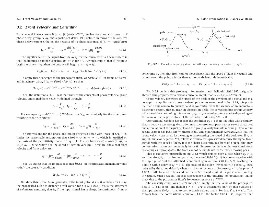
Fig. 3.2.1 Causal pulse propagation, but with superluminal group velocity (vg > c).
some time t0, then that front cannot move faster than the speed of light in vacuum andcannot reach the point z faster than z/c seconds later. Mathematically,
E(0, t)= 0 for t < t0 ⇒ E(z, t)= 0 for t < t0 + zc (3.2.8)
Fig. 3.2.1 depicts this property. Sommerfeld and Brillouin [192,1287] originallyshowed this property for a causal sinusoidal input, that is, E(0, t)= ejω0tu(t).
Group velocity describes the speed of the peak of the envelope of a signal and is aconcept that applies only to narrow-band pulses. As mentioned in Sec. 1.18, it is possi-ble that if this narrow frequency band is concentrated in the vicinity of an anomalousdispersion region, that is, near an absorption peak, the corresponding group velocitywill exceed the speed of light in vacuum, vg > c, or even become negative depending onthe value of the negative slope of the refractive index dnr/dω < 0.
Conventional wisdom has it that the condition vg > c is not at odds with relativitytheory because the strong absorption near the resonance peak causes severe distortionand attenuation of the signal peak and the group velocity loses its meaning. However, inrecent years it has been shown theoretically and experimentally [266,267,285] that thegroup velocity can retain its meaning as representing the speed of the peak even if vg issuperluminal or negative. Yet, relativistic causality is preserved because the signal fronttravels with the speed of light. It is the sharp discontinuous front of a signal that mayconvey information, not necessarily its peak. Because the pulse undergoes continuousreshaping as it propagates, the front cannot be overtaken by the faster moving peak.
This is explained pictorially in Fig. 3.2.1 which depicts such a case where vg > c,and therefore, tg < tf . For comparison, the actual field E(z, t) is shown together withthe input pulse as if the latter had been traveling in vacuum, E(0, t−z/c), reaching thepoint z with a delay of tf = z/c. The peak of the pulse, traveling with speed vg, getsdelayed by the group delay tg when it arrives at distance z. Because tg < tf , the peak ofE(z, t) shifts forward in time and occurs earlier than it would if the pulse were travelingin vacuum. Such peak shifting is a consequence of the “filtering” or “rephasing” takingplace due to the propagator filter’s frequency response e−jk(ω)z.
The causality conditions (3.2.7) and (3.2.8) imply that the value of the propagatedfield E(z, t) at some time instant t > t0 + z/c is determined only by those values ofthe input pulse E(0, t′) that are z/c seconds earlier, that is, for t0 ≤ t′ ≤ t − z/c. Thisfollows from the convolutional equation (3.1.7): the factor h(z, t − t′) requires that
3.2. Front Velocity and Causality 87
t − t′ ≥ z/c, the factor E(0, t′) requires t′ ≥ t0, yielding t0 ≤ t′ ≤ t − z/c. Thus,
E(z, t)=∫ t−z/ct0
h(z, t − t′)E(0, t′)dt′ , for t > t0 + z/c (3.2.9)
For example, the value of E(z, t) at t = t1 + tf = t1 + z/c is given by:
E(z, t1 + tf )=∫ t1t0h(z, t1 + tf − t′)E(0, t′)dt′
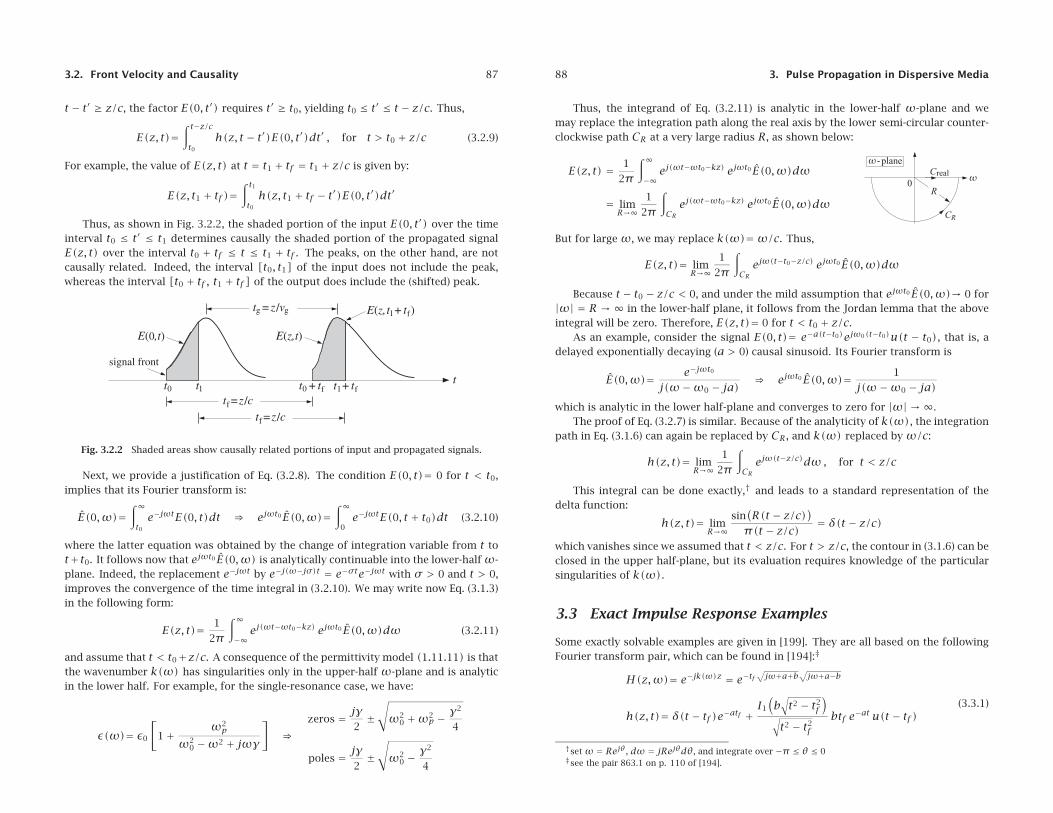
Thus, as shown in Fig. 3.2.2, the shaded portion of the input E(0, t′) over the timeinterval t0 ≤ t′ ≤ t1 determines causally the shaded portion of the propagated signalE(z, t) over the interval t0 + tf ≤ t ≤ t1 + tf . The peaks, on the other hand, are notcausally related. Indeed, the interval [t0, t1] of the input does not include the peak,whereas the interval [t0 + tf , t1 + tf ] of the output does include the (shifted) peak.
Fig. 3.2.2 Shaded areas show causally related portions of input and propagated signals.
Next, we provide a justification of Eq. (3.2.8). The condition E(0, t)= 0 for t < t0,implies that its Fourier transform is:
E(0,ω)=∫∞t0e−jωtE(0, t)dt ⇒ ejωt0 E(0,ω)=
∫∞0e−jωtE(0, t + t0)dt (3.2.10)
where the latter equation was obtained by the change of integration variable from t tot+t0. It follows now that ejωt0 E(0,ω) is analytically continuable into the lower-halfω-plane. Indeed, the replacement e−jωt by e−j(ω−jσ)t = e−σte−jωt with σ > 0 and t > 0,improves the convergence of the time integral in (3.2.10). We may write now Eq. (3.1.3)in the following form:
E(z, t)= 1
2π
∫∞−∞ej(ωt−ωt0−kz) ejωt0 E(0,ω)dω (3.2.11)
and assume that t < t0+z/c. A consequence of the permittivity model (1.11.11) is thatthe wavenumber k(ω) has singularities only in the upper-half ω-plane and is analyticin the lower half. For example, for the single-resonance case, we have:
ε(ω)= ε0
[1+ ω2
p
ω20 −ω2 + jωγ
]⇒
zeros = jγ2±√ω2
0 +ω2p − γ
2
4
poles = jγ2±√ω2
0 −γ2
4
88 3. Pulse Propagation in Dispersive Media
Thus, the integrand of Eq. (3.2.11) is analytic in the lower-half ω-plane and wemay replace the integration path along the real axis by the lower semi-circular counter-clockwise path CR at a very large radius R, as shown below:
E(z, t) = 1
2π
∫∞−∞ej(ωt−ωt0−kz) ejωt0 E(0,ω)dω
= limR→∞
1
2π
∫CRej(ωt−ωt0−kz) ejωt0 E(0,ω)dω
But for large ω, we may replace k(ω)=ω/c. Thus,
E(z, t)= limR→∞
1
2π
∫CRejω(t−t0−z/c) ejωt0 E(0,ω)dω
Because t − t0 − z/c < 0, and under the mild assumption that ejωt0 E(0,ω)→ 0 for|ω| = R → ∞ in the lower-half plane, it follows from the Jordan lemma that the aboveintegral will be zero. Therefore, E(z, t)= 0 for t < t0 + z/c.
As an example, consider the signal E(0, t)= e−a(t−t0)ejω0(t−t0)u(t − t0), that is, adelayed exponentially decaying (a > 0) causal sinusoid. Its Fourier transform is
E(0,ω)= e−jωt0j(ω−ω0 − ja) ⇒ ejωt0 E(0,ω)= 1
j(ω−ω0 − ja)which is analytic in the lower half-plane and converges to zero for |ω| → ∞.
The proof of Eq. (3.2.7) is similar. Because of the analyticity of k(ω), the integrationpath in Eq. (3.1.6) can again be replaced by CR, and k(ω) replaced by ω/c:
h(z, t)= limR→∞
1
2π
∫CRejω(t−z/c)dω , for t < z/c
This integral can be done exactly,† and leads to a standard representation of thedelta function:
h(z, t)= limR→∞
sin(R(t − z/c))π(t − z/c) = δ(t − z/c)
which vanishes since we assumed that t < z/c. For t > z/c, the contour in (3.1.6) can beclosed in the upper half-plane, but its evaluation requires knowledge of the particularsingularities of k(ω).
3.3 Exact Impulse Response Examples
Some exactly solvable examples are given in [199]. They are all based on the followingFourier transform pair, which can be found in [194]:‡
H(z,ω)= e−jk(ω)z = e−tf√jω+a+b
√jω+a−b
h(z, t)= δ(t − tf )e−atf +I1(b√t2 − t2f
)√t2 − t2f
btf e−at u(t − tf )(3.3.1)
†set ω = Rejθ, dω = jRejθdθ, and integrate over −π ≤ θ ≤ 0‡see the pair 863.1 on p. 110 of [194].
3.3. Exact Impulse Response Examples 89
where I1(x) is the modified Bessel function of the first kind of order one, and tf = z/cis the front delay. The unit step u(t− tf ) enforces the causality condition (3.2.7). Fromthe expression of H(z,ω), we identify the corresponding wavenumber:
k(ω)= −jc
√jω+ a+ b
√jω+ a− b (3.3.2)
The following physical examples are described by appropriate choices of the param-eters a,b, c in Eq. (3.3.2):
1. a = 0 , b = 0 − propagation in vacuum or dielectric2. a > 0 , b = 0 − weakly conducting dielectric3. a = b > 0 − medium with finite conductivity4. a = 0 , b = jωp − lossless plasma5. a = 0 , b = jωc − hollow metallic waveguide6. a+ b = R′/L′ , a− b = G′/C′ − lossy transmission line
The anti-hermitian property k(−ω)∗= −k(ω) is satisfied in two cases: when theparameters a,b are both real, or, when a is real and b imaginary.
In case 1, we have k =ω/c and h(z, t)= δ(t− tf )= δ(t− z/c). Setting a = cα > 0and b = 0, we find for case 2:
k = ω− jac
= ωc− jα (3.3.3)
which corresponds to a medium with a constant attenuation coefficient α = a/c anda propagation constant β = ω/c, as was the case of a weakly conducting dielectric ofSec. 2.7. In this case c is the speed of light in the dielectric, i.e. c = 1/√με and a isrelated to the conductivity σ by a = cα = σ/2ε. The medium impulse response is:
h(z, t)= δ(t − tf )e−atf = δ(t − z/c)e−αz
Eq. (3.1.7) then implies that an input signal will travel at speed c while attenuatingwith distance:
E(z, t)= e−αzE(0, t − z/c)Case 3 describes a medium with frequency-independent permittivity and conductiv-
ity ε,σ with the parameters a = b = σ/2ε and c = 1/√μ0ε. Eq. (3.3.2) becomes:
k = ωc
√1− j σ
ωε(3.3.4)
and the impulse response is:
h(z, t)= δ(t − z/c)e−az/c +I1(a√t2 − (z/c)2
)√t2 − (z/c)2
azce−at u(t − z/c) (3.3.5)
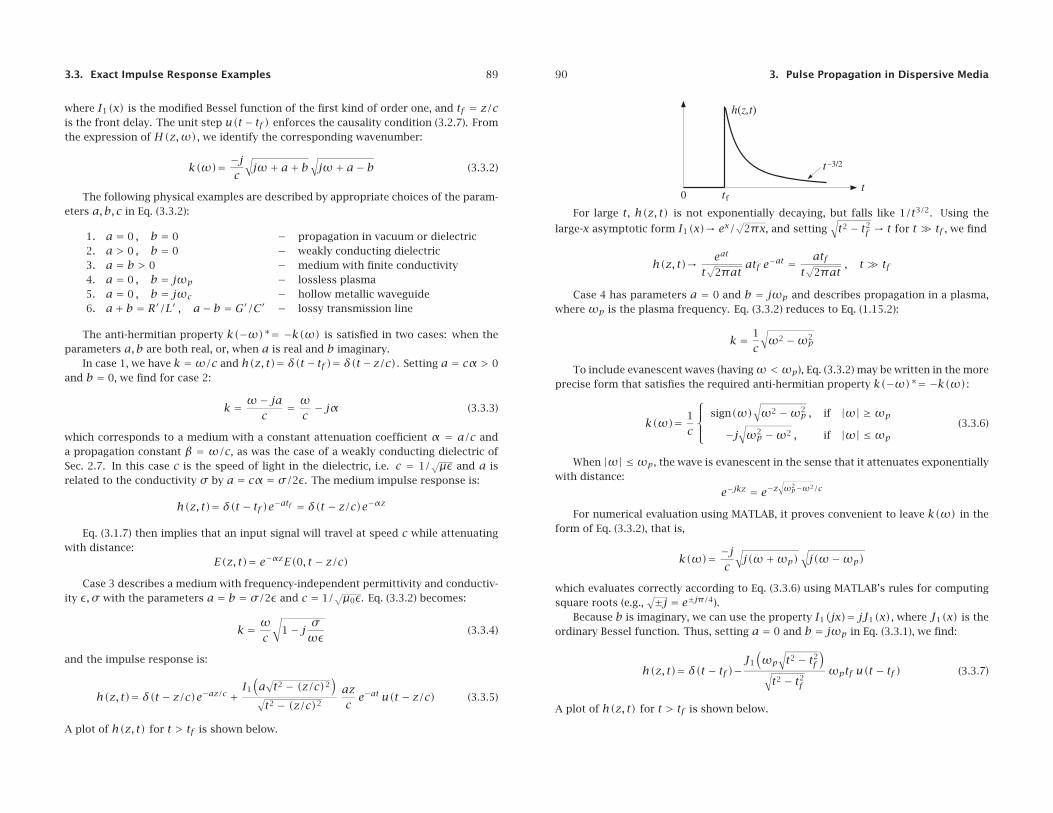
A plot of h(z, t) for t > tf is shown below.
90 3. Pulse Propagation in Dispersive Media
For large t, h(z, t) is not exponentially decaying, but falls like 1/t3/2. Using the
large-x asymptotic form I1(x)→ ex/√
2πx, and setting√t2 − t2f → t for t� tf , we find
h(z, t)→ eat
t√
2πatatf e−at = atf
t√
2πat, t� tf
Case 4 has parameters a = 0 and b = jωp and describes propagation in a plasma,where ωp is the plasma frequency. Eq. (3.3.2) reduces to Eq. (1.15.2):
k = 1
c
√ω2 −ω2
p
To include evanescent waves (havingω <ωp), Eq. (3.3.2) may be written in the moreprecise form that satisfies the required anti-hermitian property k(−ω)∗= −k(ω):
k(ω)= 1
c
⎧⎪⎨⎪⎩
sign(ω)√ω2 −ω2
p , if |ω| ≥ωp
−j√ω2p −ω2 , if |ω| ≤ωp
(3.3.6)
When |ω| ≤ωp, the wave is evanescent in the sense that it attenuates exponentiallywith distance:
e−jkz = e−z√ω2p−ω2/c
For numerical evaluation using MATLAB, it proves convenient to leave k(ω) in theform of Eq. (3.3.2), that is,
k(ω)= −jc
√j(ω+ωp)
√j(ω−ωp)
which evaluates correctly according to Eq. (3.3.6) using MATLAB’s rules for computingsquare roots (e.g.,
√±j = e±jπ/4).Because b is imaginary, we can use the property I1(jx)= jJ1(x), where J1(x) is the
ordinary Bessel function. Thus, setting a = 0 and b = jωp in Eq. (3.3.1), we find:
h(z, t)= δ(t − tf )−J1
(ωp
√t2 − t2f
)√t2 − t2f
ωptf u(t − tf ) (3.3.7)
A plot of h(z, t) for t > tf is shown below.
3.4. Transient and Steady-State Behavior 91
The propagated output E(z, t) due to a causal input, E(0, t)= E(0, t)u(t), is ob-tained by convolution, where we must impose the conditions t′ ≥ tf and t − t′ ≥ 0:
E(z, t)=∫∞−∞h(z, t′)E(0, t − t′)dt′
which for t ≥ tf leads to:
E(z, t)= E(0, t − tf )−∫ ttf
J1
(ωp
√t′2 − t2f
)√t′2 − t2f
ωptf E(0, t − t′)dt′ (3.3.8)
We shall use Eq. (3.3.8) in the next section to illustrate the transient and steady-state response of a propagation medium such as a plasma or a waveguide. The large-tbehavior of h(z, t) is obtained from the asymptotic form:
J1(x)→√
2
πxcos
(x− 3π
4
), x� 1
which leads to
h(z, t)→ −√
2ωp tf√πt3/2
cos(ωpt − 3π
4
), t� tf (3.3.9)
Case 5 is the same as case 4, but describes propagation in an air-filled hollow metallicwaveguide with cutoff frequencyωc. We will see in Chap. 9 that the dispersion relation-ship (3.3.6) is a consequence of the boundary conditions on the waveguide walls, andtherefore, it is referred to as waveguide dispersion, as opposed to material dispersionarising from a frequency-dependent permittivity ε(ω).
Case 6 describes a lossy transmission line (see Sec. 11.6) with distributed (that is, perunit length) inductance L′, capacitance C′, series resistance R′, and shunt conductanceG′. This case reduces to case 3 if G′ = 0. The corresponding propagation speed isc = 1/
√L′C′. Theω–k dispersion relationship can be written in the form of Eq. (11.6.5):
k = −j√(R′ + jωL′)(G′ + jωC′) =ω
√L′C′
√(1− j R
′
ωL′
)(1− j G
′
ωC′
)
3.4 Transient and Steady-State Behavior
The frequency response e−jk(ω)z is the Fourier transform of h(z, t), but because of thecausality condition h(z, t)= 0 for t < z/c, the time-integration in this Fourier transformcan be restricted to the interval z/c < t <∞, that is,
e−jk(ω)z =∫∞z/ce−jωth(z, t)dt (3.4.1)
92 3. Pulse Propagation in Dispersive Media
We mention, parenthetically, that Eq. (3.4.1), which incorporates the causality con-dition of h(z, t), can be used to derive the lower half-plane analyticity of k(ω) and ofthe corresponding complex refractive index n(ω) defined through k(ω)= ωn(ω)/c.The analyticity properties of n(ω) can then be used to derive the Kramers-Kronig dis-persion relations satisfied by n(ω) itself [197], as opposed to those satisfied by thesusceptibility χ(ω) that were discussed in Sec. 1.17.
When a causal sinusoidal input is applied to the linear system h(z, t), we expect thesystem to exhibit an initial transient behavior followed by the usual sinusoidal steady-state response. Indeed, applying the initial pulse E(0, t)= ejω0tu(t), we obtain fromthe system’s convolutional equation:
E(z, t)=∫ tz/ch(z, t′)E(0, t − t′)dt′ =
∫ tz/ch(z, t′)ejω0(t−t′)dt′
where the restricted limits of integration follow from the conditions t′ ≥ z/c and t−t′ ≥0 as required by the arguments of the functions h(z, t′) and E(0, t − t′). Thus, fort ≥ z/c, the propagated field takes the form:
E(z, t)= ejω0t∫ tz/ce−jω0t′h(z, t′)dt′ (3.4.2)
In the steady-state limit, t → ∞, the above integral tends to the frequency response(3.4.1) evaluated at ω =ω0, resulting in the standard sinusoidal response:
ejω0t∫ tz/ce−jω0t′h(z, t′)dt′ → ejω0t
∫∞z/ce−jω0t′h(z, t′)dt′ = H(z,ω0)ejω0t , or,
Esteady(z, t)= ejω0t−jk(ω0)z , for t� z/c (3.4.3)
Thus, the field E(z, t) eventually evolves into an ordinary plane wave at frequencyω0 and wavenumber k(ω0)= β(ω0)−jα(ω0). The initial transients are given by theexact equation (3.4.2) and depend on the particular form of k(ω). They are generallyreferred to as “precursors” or “forerunners” and were originally studied by Sommerfeldand Brillouin [192,1287] for the case of a single-resonance Lorentz permittivity model.
It is beyond the scope of this book to study the precursors of the Lorentz model.However, we may use the exactly solvable model for a plasma or waveguide given inEq. (3.3.7) and numerically integrate (3.4.2) to illustrate the transient and steady-statebehavior.
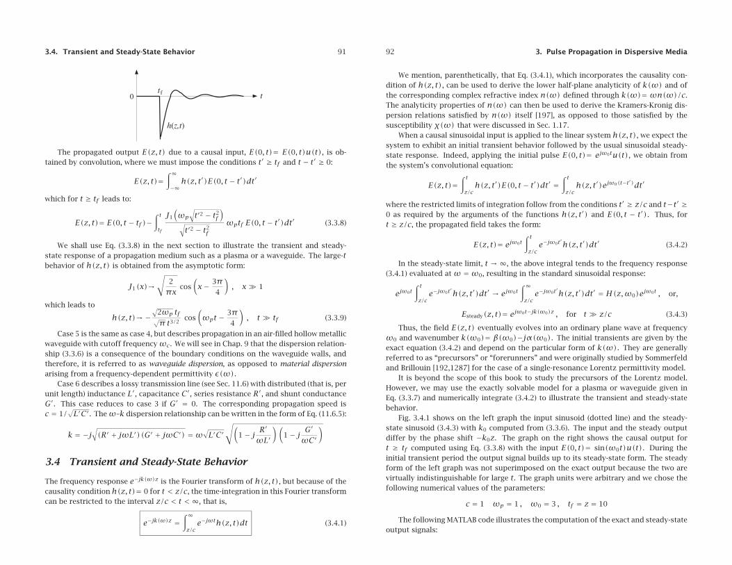
Fig. 3.4.1 shows on the left graph the input sinusoid (dotted line) and the steady-state sinusoid (3.4.3) with k0 computed from (3.3.6). The input and the steady outputdiffer by the phase shift −k0z. The graph on the right shows the causal output fort ≥ tf computed using Eq. (3.3.8) with the input E(0, t)= sin(ω0t)u(t). During theinitial transient period the output signal builds up to its steady-state form. The steadyform of the left graph was not superimposed on the exact output because the two arevirtually indistinguishable for large t. The graph units were arbitrary and we chose thefollowing numerical values of the parameters:
c = 1 ωp = 1 , ω0 = 3 , tf = z = 10
The following MATLAB code illustrates the computation of the exact and steady-stateoutput signals:
3.4. Transient and Steady-State Behavior 93
0 10 20 30 40
−1
0
1
t
input and steady− state output
tf
0 10 20 30 40
−1
0
1
t
exact output
tf
Fig. 3.4.1 Transient and steady-state sinusoidal response.
wp = 1; w0 = 3; tf = 10;k0 = -j * sqrt(j*(w0+wp)) * sqrt(j*(w0-wp)); % equivalent to Eq. (3.3.6)
t = linspace(0,40, 401);
N = 15; K = 20; % use N-point Gaussian quadrature, dividing [tf , t] into K subintervals
for i=1:length(t),if t(i)<tf,
Ez(i) = 0;Es(i) = 0;
else[w,x] = quadrs(linspace(tf,t(i),K), N); % quadrature weights and points
h = - wp^2 * tf * J1over(wp*sqrt(x.^2 - tf^2)) .* exp(j*w0*(t(i)-x));Ez(i) = exp(j*w0*(t(i)-tf)) + w’*h; % exact output
Es(i) = exp(j*w0*t(i)-j*k0*tf); % steady-state
endend
es = imag(Es); ez = imag(Ez); % input is E(0, t) = sin(ω0t) u(t)
figure; plot(t,es); figure; plot(t,ez);
The code uses the function quadrs (see Appendix L) to compute the integral over theinterval [tf , t], dividing this interval into K subintervals and using an N-point Gauss-Legendre quadrature method on each subinterval.
We wrote a function J1over to implement the function J1(x)/x. The function usesthe power series expansion, J1(x)/x = 0.5(1 − x2/8 + x4/192), for small x, and thebuilt-in MATLAB function besselj for larger x:
function y = J1over(x)
y = zeros(size(x)); % y has the same size as x
xmin = 1e-4;
i = find(abs(x) < xmin);
94 3. Pulse Propagation in Dispersive Media
y(i) = 0.5 * (1 - x(i).^2 / 8 + x(i).^4 / 192);
i = find(abs(x) >= xmin);y(i) = besselj(1, x(i)) ./ x(i);
0 10 20 30 40 50 60 70 80 90 100
−1
0
1
t
input and steady− state evanescent output
tf
0 10 20 30 40 50 60 70 80 90 100
−1
0
1
t
exact evanescent output
tf
Fig. 3.4.2 Transient and steady-state response for evanescent sinusoids.
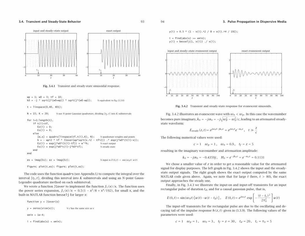
Fig. 3.4.2 illustrates an evanescent wave withω0 < ωp. In this case the wavenumber
becomes pure imaginary, k0 = −jα0 = −j√ω2p −ω2
0/c, leading to an attenuated steady-state waveform:
Esteady(z, t)= ejω0t−jk0z = ejω0te−α0z , t� zc
The following numerical values were used:
c = 1 ωp = 1 , ω0 = 0.9 , tf = z = 5
resulting in the imaginary wavenumber and attenuation amplitude:
k0 = −jα0 = −0.4359j , H0 = e−jk0z = e−αoz = 0.1131
We chose a smaller value of z in order to get a reasonable value for the attenuatedsignal for display purposes. The left graph in Fig. 3.4.2 shows the input and the steady-state output signals. The right graph shows the exact output computed by the sameMATLAB code given above. Again, we note that for large t (here, t > 80), the exactoutput approaches the steady one.
Finally, in Fig. 3.4.3 we illustrate the input-on and input-off transients for an inputrectangular pulse of duration td, and for a causal gaussian pulse, that is,
E(0, t)= sin(ω0t)[u(t)−u(t − td)
], E(0, t)= ejω0t exp
[−(t − tc)
2
2τ20
]u(t)
The input-off transients for the rectangular pulse are due to the oscillating and de-caying tail of the impulse response h(z, t) given in (3.3.9). The following values of theparameters were used:
c = 1 ωp = 1 , ω0 = 3 , tf = z = 30 , td = 20 , tc = τ0 = 5
3.5. Pulse Propagation and Group Velocity 95
0 10 20 30 40 50 60 70 80
−1
0
1
t
propagation of rectangular pulse
tf
input output
0 10 20 30 40 50 60 70 80
−1
0
1
t
propagation of gaussian pulse
tf
input output
Fig. 3.4.3 Rectangular and gaussian pulse propagation.
The MATLAB code for the rectangular pulse case is essentially the same as aboveexcept that it uses the function upulse to enforce the finite pulse duration:
wp = 1; w0 = 3; tf = 30; td = 20; N = 15; K = 20;k0 = -j * sqrt(j*(w0+wp)) * sqrt(j*(w0-wp));
t = linspace(0,80,801);
E0 = exp(j*w0*t) .* upulse(t,td);
for i=1:length(t),if t(i)<tf,Ez(i) = 0;
else[w,x] = quadrs(linspace(tf,t(i),K), N);h = - wp^2 * tf * J1over(wp*sqrt(x.^2-tf^2)) .* ...
exp(j*w0*(t(i)-x)) .* upulse(t(i)-x,td);Ez(i) = exp(j*w0*(t(i)-tf)).*upulse(t(i)-tf,td) + w’*h;
endend
e0 = imag(E0); ez = imag(Ez);
plot(t,ez,’-’, t,e0,’-’);
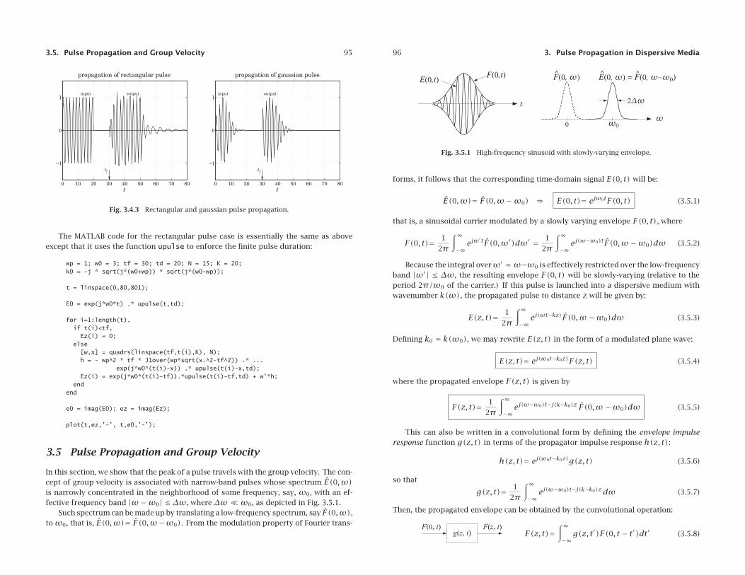
3.5 Pulse Propagation and Group Velocity
In this section, we show that the peak of a pulse travels with the group velocity. The con-cept of group velocity is associated with narrow-band pulses whose spectrum E(0,ω)is narrowly concentrated in the neighborhood of some frequency, say, ω0, with an ef-fective frequency band |ω−ω0| ≤ Δω, where Δω ω0, as depicted in Fig. 3.5.1.
Such spectrum can be made up by translating a low-frequency spectrum, say F(0,ω),toω0, that is, E(0,ω)= F(0,ω−ω0). From the modulation property of Fourier trans-
96 3. Pulse Propagation in Dispersive Media
Fig. 3.5.1 High-frequency sinusoid with slowly-varying envelope.
forms, it follows that the corresponding time-domain signal E(0, t) will be:
E(0,ω)= F(0,ω−ω0) ⇒ E(0, t)= ejω0tF(0, t) (3.5.1)
that is, a sinusoidal carrier modulated by a slowly varying envelope F(0, t), where
F(0, t)= 1
2π
∫∞−∞ejω
′tF(0,ω′)dω′ = 1
2π
∫∞−∞ej(ω−ω0)tF(0,ω−ω0)dω (3.5.2)
Because the integral overω′ =ω−ω0 is effectively restricted over the low-frequencyband |ω′| ≤ Δω, the resulting envelope F(0, t) will be slowly-varying (relative to theperiod 2π/ω0 of the carrier.) If this pulse is launched into a dispersive medium withwavenumber k(ω), the propagated pulse to distance z will be given by:
E(z, t)= 1
2π
∫∞−∞ej(ωt−kz)F(0,ω−ω0)dω (3.5.3)
Defining k0 = k(ω0), we may rewrite E(z, t) in the form of a modulated plane wave:
E(z, t)= ej(ω0t−k0z)F(z, t) (3.5.4)
where the propagated envelope F(z, t) is given by
F(z, t)= 1
2π
∫∞−∞ej(ω−ω0)t−j(k−k0)z F(0,ω−ω0)dω (3.5.5)
This can also be written in a convolutional form by defining the envelope impulseresponse function g(z, t) in terms of the propagator impulse response h(z, t):
h(z, t)= ej(ω0t−k0z)g(z, t) (3.5.6)
so that
g(z, t)= 1
2π
∫∞−∞ej(ω−ω0)t−j(k−k0)z dω (3.5.7)
Then, the propagated envelope can be obtained by the convolutional operation:
F(z, t)=∫∞−∞g(z, t′)F(0, t − t′)dt′ (3.5.8)
3.5. Pulse Propagation and Group Velocity 97
Because F(0,ω −ω0) restricts the effective range of integration in Eq. (3.5.5) to anarrow band aboutω0, one can expand k(ω) to a Taylor series aboutω0 and keep onlythe first few terms:
k(ω)= k0 + k′0(ω−ω0)+1
2k′′0 (ω−ω0)2+· · · (3.5.9)
where
k0 = k(ω0) , k′0 =dkdω
∣∣∣∣ω0
, k′′0 =d2kdω2
∣∣∣∣∣ω0
(3.5.10)
If k(ω) is real, we recognize k′0 as the inverse of the group velocity at frequency ω0:
k′0 =dkdω
∣∣∣∣ω0
= 1
vg(3.5.11)
If k′0 is complex-valued, k′0 = β′0 − jα′0, then its real part determines the group velocitythrough β′0 = 1/vg, or, vg = 1/β′0. The second derivative k′′0 is referred to as the“dispersion coefficient” and is responsible for the spreading and chirping of the wavepacket, as we see below.
Keeping up to the quadratic term in the quantity k(ω)−k0 in (3.5.5), and changingintegration variables to ω′ =ω−ω0, we obtain the approximation:
F(z, t)= 1
2π
∫∞−∞ejω
′(t−k′0z)−jk′′0 zω′2/2F(0,ω′)dω′ (3.5.12)
In the linear approximation, we may keep k′0 and ignore the k′′0 term, and in thequadratic approximation, we keep both k′0 and k′′0 . For the linear case, we have bycomparing with Eq. (3.5.2):
F(z, t)= 1
2π
∫∞−∞ejω
′(t−k′0z)F(0,ω′)dω′ = F(0, t − k′0z) (3.5.13)
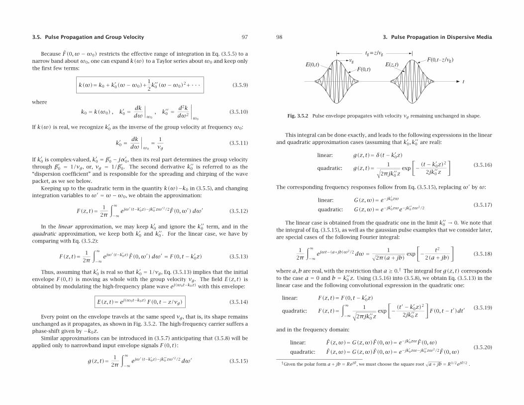
Thus, assuming that k′0 is real so that k′0 = 1/vg, Eq. (3.5.13) implies that the initialenvelope F(0, t) is moving as whole with the group velocity vg. The field E(z, t) isobtained by modulating the high-frequency plane wave ej(ω0t−k0z) with this envelope:
E(z, t)= ej(ω0t−k0z) F(0, t − z/vg) (3.5.14)
Every point on the envelope travels at the same speed vg, that is, its shape remainsunchanged as it propagates, as shown in Fig. 3.5.2. The high-frequency carrier suffers aphase-shift given by −k0z.
Similar approximations can be introduced in (3.5.7) anticipating that (3.5.8) will beapplied only to narrowband input envelope signals F(0, t):
g(z, t)= 1
2π
∫∞−∞ejω
′(t−k′0z)−jk′′0 zω′2/2 dω′ (3.5.15)
98 3. Pulse Propagation in Dispersive Media
Fig. 3.5.2 Pulse envelope propagates with velocity vg remaining unchanged in shape.
This integral can be done exactly, and leads to the following expressions in the linearand quadratic approximation cases (assuming that k′0, k′′0 are real):
linear: g(z, t)= δ(t − k′0z)
quadratic: g(z, t)= 1√2πjk′′0 z
exp
[−(t − k
′0z)2
2jk′′0 z
](3.5.16)
The corresponding frequency responses follow from Eq. (3.5.15), replacing ω′ by ω:
linear: G(z,ω)= e−jk′0zωquadratic: G(z,ω)= e−jk′0zωe−jk′′0 zω2/2 (3.5.17)
The linear case is obtained from the quadratic one in the limit k′′0 → 0. We note thatthe integral of Eq. (3.5.15), as well as the gaussian pulse examples that we consider later,are special cases of the following Fourier integral:
1
2π
∫∞−∞ejωt−(a+jb)ω
2/2 dω = 1√2π(a+ jb) exp
[− t2
2(a+ jb)
](3.5.18)
where a,b are real, with the restriction that a ≥ 0.† The integral for g(z, t) correspondsto the case a = 0 and b = k′′0 z. Using (3.5.16) into (3.5.8), we obtain Eq. (3.5.13) in thelinear case and the following convolutional expression in the quadratic one:
linear: F(z, t)= F(0, t − k′0z)
quadratic: F(z, t)=∫∞−∞
1√2πjk′′0 z
exp
[−(t
′ − k′0z)2
2jk′′0 z
]F(0, t − t′)dt′ (3.5.19)
and in the frequency domain:
linear: F(z,ω)= G(z,ω)F(0,ω)= e−jk′0zωF(0,ω)quadratic: F(z,ω)= G(z,ω)F(0,ω)= e−jk′0zω−jk′′0 zω2/2F(0,ω)
(3.5.20)
†Given the polar form a+ jb = Rejθ, we must choose the square root√a+ jb = R1/2ejθ/2 .
3.6. Group Velocity Dispersion and Pulse Spreading 99
3.6 Group Velocity Dispersion and Pulse Spreading
In the linear approximation, the envelope propagates with the group velocity vg, re-maining unchanged in shape. But in the quadratic approximation, as a consequence ofEq. (3.5.19), it spreads and reduces in amplitude with distance z, and it chirps. To seethis, consider a gaussian input pulse of effective width τ0:
F(0, t)= exp
[− t2
2τ20
]⇒ E(0, t)= ejω0tF(0, t)= ejω0t exp
[− t2
2τ20
](3.6.1)
with Fourier transforms F(0,ω) and E(0,ω)= F(0,ω−ω0):
F(0,ω)=√
2πτ20 e−τ
20ω2/2 ⇒ E(0,ω)=
√2πτ2
0 e−τ20(ω−ω0)2/2 (3.6.2)
with an effective width Δω = 1/τ0. Thus, the condition Δω ω0 requires thatτ0ω0 � 1, that is, an envelope with a long duration relative to the carrier’s period.
The propagated envelope F(z, t) can be determined either from Eq. (3.5.19) or from(3.5.20). Using the latter, we have:
F(z,ω)=√
2πτ20 e−jk
′0zω−jk′′0 zω2/2e−τ
20ω2/2 =
√2πτ2
0 e−jk′0zωe−(τ
20+jk′′0 z)ω2/2 (3.6.3)
The Fourier integral (3.5.18), then, gives the propagated envelope in the time domain:
F(z, t)=√√√√ τ2
0
τ20 + jk′′0 z
exp
[− (t − k′0z)2
2(τ20 + jk′′0 z)
](3.6.4)
Thus, effectively we have the replacementτ20 → τ2
0+jk′′0 z. Assuming for the momentthat k′0 and k′′0 are real, we find for the magnitude of the propagated pulse:
|F(z, t)| =[
τ40
τ40 + (k′′0 z)2
]1/4
exp
[− (t − k′0z)2 τ2
0
2(τ4
0 + (k′′0 z)2)]
(3.6.5)
where we used the property |τ20 + jk′′0 z| =
√τ4
0 + (k′′0 z)2. The effective width is deter-mined from the argument of the exponent to be:
τ2 = τ40 + (k′′0 z)2
τ20
⇒ τ =⎡⎣τ2
0 +(k′′0 zτ0
)2⎤⎦
1/2
(3.6.6)
Therefore, the pulse width increases with distance z. Also, the amplitude of thepulse decreases with distance, as measured for example at the peak maximum:
|F|max =[
τ40
τ40 + (k′′0 z)2
]1/4
The peak maximum occurs at the group delay t = k′0z, and hence it is moving at thegroup velocity vg = 1/k′0.
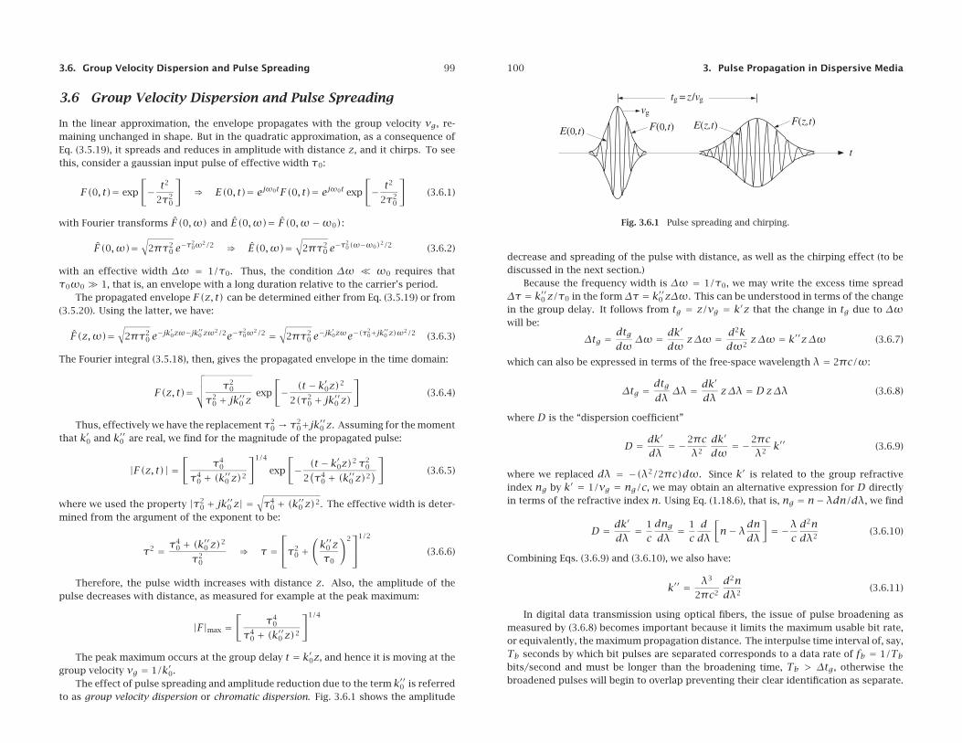
The effect of pulse spreading and amplitude reduction due to the term k′′0 is referredto as group velocity dispersion or chromatic dispersion. Fig. 3.6.1 shows the amplitude
100 3. Pulse Propagation in Dispersive Media
Fig. 3.6.1 Pulse spreading and chirping.
decrease and spreading of the pulse with distance, as well as the chirping effect (to bediscussed in the next section.)
Because the frequency width is Δω = 1/τ0, we may write the excess time spreadΔτ = k′′0 z/τ0 in the formΔτ = k′′0 zΔω. This can be understood in terms of the changein the group delay. It follows from tg = z/vg = k′z that the change in tg due to Δωwill be:
Δtg = dtgdω
Δω = dk′
dωzΔω = d2k
dω2zΔω = k′′zΔω (3.6.7)
which can also be expressed in terms of the free-space wavelength λ = 2πc/ω:
Δtg = dtgdλ
Δλ = dk′
dλzΔλ = DzΔλ (3.6.8)
where D is the “dispersion coefficient”
D = dk′
dλ= −2πc
λ2
dk′
dω= −2πc
λ2k′′ (3.6.9)
where we replaced dλ = −(λ2/2πc)dω. Since k′ is related to the group refractiveindex ng by k′ = 1/vg = ng/c, we may obtain an alternative expression for D directlyin terms of the refractive index n. Using Eq. (1.18.6), that is, ng = n− λdn/dλ, we find
D = dk′
dλ= 1
cdngdλ
= 1
cddλ
[n− λdn
dλ
]= −λ
cd2ndλ2
(3.6.10)
Combining Eqs. (3.6.9) and (3.6.10), we also have:
k′′ = λ3
2πc2
d2ndλ2
(3.6.11)
In digital data transmission using optical fibers, the issue of pulse broadening asmeasured by (3.6.8) becomes important because it limits the maximum usable bit rate,or equivalently, the maximum propagation distance. The interpulse time interval of, say,Tb seconds by which bit pulses are separated corresponds to a data rate of fb = 1/Tbbits/second and must be longer than the broadening time, Tb > Δtg, otherwise thebroadened pulses will begin to overlap preventing their clear identification as separate.
3.6. Group Velocity Dispersion and Pulse Spreading 101
This limits the propagation distance z to a maximum value:†
DzΔλ ≤ Tb = 1
fb⇒ z ≤ 1
fb DΔλ= 1
fb k′′Δω(3.6.12)
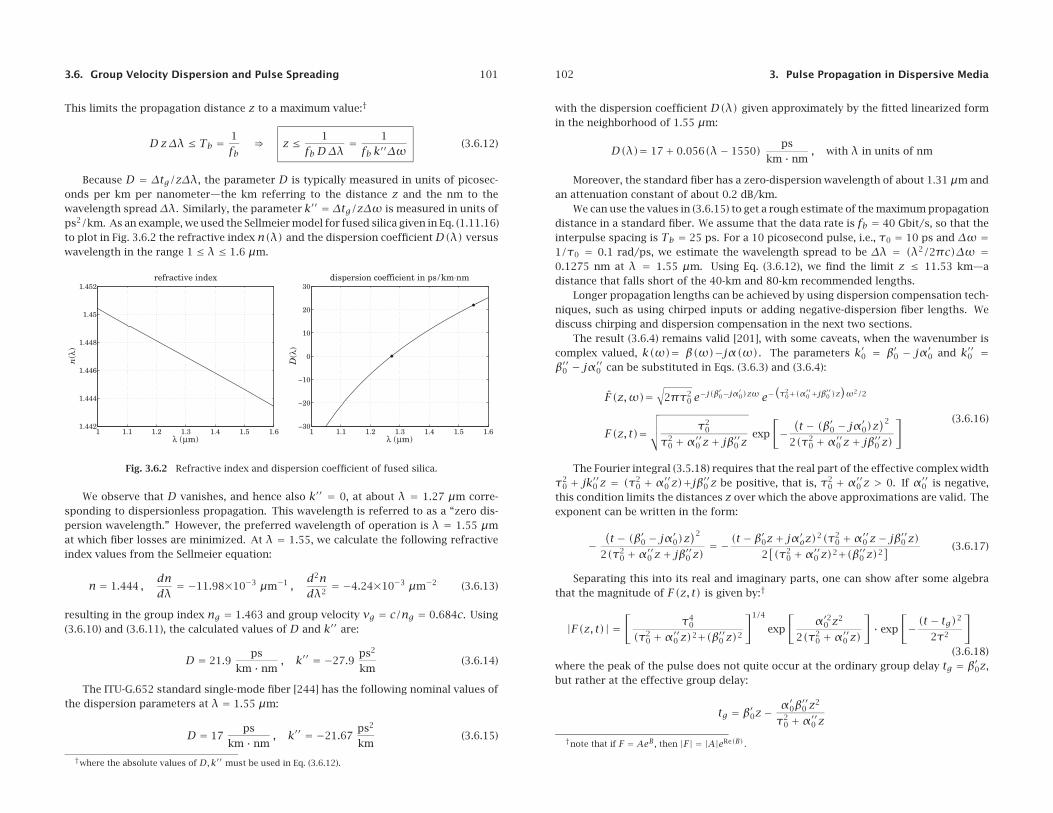
Because D = Δtg/zΔλ, the parameter D is typically measured in units of picosec-onds per km per nanometer—the km referring to the distance z and the nm to thewavelength spread Δλ. Similarly, the parameter k′′ = Δtg/zΔω is measured in units ofps2/km. As an example, we used the Sellmeier model for fused silica given in Eq. (1.11.16)to plot in Fig. 3.6.2 the refractive index n(λ) and the dispersion coefficientD(λ) versuswavelength in the range 1 ≤ λ ≤ 1.6 μm.
1 1.1 1.2 1.3 1.4 1.5 1.61.442
1.444
1.446
1.448
1.45
1.452
λ (μm)
n(λ
)
refractive index
1 1.1 1.2 1.3 1.4 1.5 1.6−30
−20
−10
0
10
20
30
λ (μm)
D(λ
)
dispersion coefficient in ps /km⋅nm
Fig. 3.6.2 Refractive index and dispersion coefficient of fused silica.
We observe that D vanishes, and hence also k′′ = 0, at about λ = 1.27 μm corre-sponding to dispersionless propagation. This wavelength is referred to as a “zero dis-persion wavelength.” However, the preferred wavelength of operation is λ = 1.55 μmat which fiber losses are minimized. At λ = 1.55, we calculate the following refractiveindex values from the Sellmeier equation:
n = 1.444 ,dndλ
= −11.98×10⁻³ μm−1 ,d2ndλ2
= −4.24×10⁻³ μm−2 (3.6.13)
resulting in the group index ng = 1.463 and group velocity vg = c/ng = 0.684c. Using(3.6.10) and (3.6.11), the calculated values of D and k′′ are:
D = 21.9ps
km · nm, k′′ = −27.9
ps2
km(3.6.14)
The ITU-G.652 standard single-mode fiber [244] has the following nominal values ofthe dispersion parameters at λ = 1.55 μm:
D = 17ps
km · nm, k′′ = −21.67
ps2
km(3.6.15)
†where the absolute values of D,k′′ must be used in Eq. (3.6.12).
102 3. Pulse Propagation in Dispersive Media
with the dispersion coefficient D(λ) given approximately by the fitted linearized formin the neighborhood of 1.55 μm:
D(λ)= 17+ 0.056(λ− 1550)ps
km · nm, with λ in units of nm
Moreover, the standard fiber has a zero-dispersion wavelength of about 1.31 μm andan attenuation constant of about 0.2 dB/km.
We can use the values in (3.6.15) to get a rough estimate of the maximum propagationdistance in a standard fiber. We assume that the data rate is fb = 40 Gbit/s, so that theinterpulse spacing is Tb = 25 ps. For a 10 picosecond pulse, i.e., τ0 = 10 ps and Δω =1/τ0 = 0.1 rad/ps, we estimate the wavelength spread to be Δλ = (λ2/2πc)Δω =0.1275 nm at λ = 1.55 μm. Using Eq. (3.6.12), we find the limit z ≤ 11.53 km—adistance that falls short of the 40-km and 80-km recommended lengths.
Longer propagation lengths can be achieved by using dispersion compensation tech-niques, such as using chirped inputs or adding negative-dispersion fiber lengths. Wediscuss chirping and dispersion compensation in the next two sections.
The result (3.6.4) remains valid [201], with some caveats, when the wavenumber iscomplex valued, k(ω)= β(ω)−jα(ω). The parameters k′0 = β′0 − jα′0 and k′′0 =β′′0 − jα′′0 can be substituted in Eqs. (3.6.3) and (3.6.4):
F(z,ω)=√
2πτ20 e−j(β
′0−jα′0)zω e−
(τ2
0+(α′′0 +jβ′′0 )z)ω2/2
F(z, t)=√√√√ τ2
0
τ20 +α′′0 z+ jβ′′0 z
exp
[−(t − (β′0 − jα′0)z
)2
2(τ20 +α′′0 z+ jβ′′0 z)
] (3.6.16)
The Fourier integral (3.5.18) requires that the real part of the effective complex widthτ2
0 + jk′′0 z = (τ20 + α′′0 z)+jβ′′0 z be positive, that is, τ2
0 + α′′0 z > 0. If α′′0 is negative,this condition limits the distances z over which the above approximations are valid. Theexponent can be written in the form:
−(t − (β′0 − jα′0)z
)2
2(τ20 +α′′0 z+ jβ′′0 z)
= −(t − β′0z+ jα′oz)2(τ2
0 +α′′0 z− jβ′′0 z)2[(τ2
0 +α′′0 z)2+(β′′0 z)2] (3.6.17)
Separating this into its real and imaginary parts, one can show after some algebrathat the magnitude of F(z, t) is given by:†
|F(z, t)| =[
τ40
(τ20 +α′′0 z)2+(β′′0 z)2
]1/4
exp
[α′20 z2
2(τ20 +α′′0 z)
]· exp
[−(t − tg)
2
2τ2
]
(3.6.18)where the peak of the pulse does not quite occur at the ordinary group delay tg = β′0z,but rather at the effective group delay:
tg = β′0z−α′0β′′0 z2
τ20 +α′′0 z
†note that if F = AeB, then |F| = |A|eRe(B).
3.7. Propagation and Chirping 103
The effective width of the peak generalizes Eq. (3.6.6)
τ2 = τ20 +α′′0 z+
(β′′0 z)2
τ20 +α′′0 z
From the imaginary part of Eq. (3.6.17), we observe two additional effects. First, thenon-zero coefficient of the jt term is equivalent to a z-dependent frequency shift of thecarrier frequency ω0, and second, from the coefficient of jt2/2, there will be a certainamount of chirping as discussed in the next section. The frequency shift and chirpingcoefficient (generalizing Eq. (3.7.6)) turn out to be:
Δω0 = − α′oz(τ20 +α′′0 z)
(τ20 +α′′0 z)2+(β′′0 z)2
, ω0 = β′′0 z(τ2
0 +α′′0 z)2+(β′′0 z)2
In most applications and in the fast and slow light experiments that have been carriedout thus far, care has been taken to minimize these effects by operating in frequencybands where α′0,α′′0 are small and by limiting the propagation distance z.
3.7 Propagation and Chirping
A chirped sinusoid has an instantaneous frequency that changes linearly with time,referred to as linear frequency modulation (FM). It is obtained by the substitution:
ejω0t → ej(ω0t+ω0t2/2) (3.7.1)
where the “chirping parameter” ω0 is a constant representing the rate of change of theinstantaneous frequency. The phaseθ(t) and instantaneous frequency θ(t)= dθ(t)/dtare for the above sinusoids:
θ(t)=ω0t → θ(t)=ω0t + 1
2ω0t2
θ(t)=ω0 → θ(t)=ω0 + ω0t(3.7.2)
The parameter ω0 can be positive or negative resulting in an increasing or decreasinginstantaneous frequency. A chirped gaussian pulse is obtained by modulating a chirpedsinusoid by a gaussian envelope:
E(0, t)= ej(ω0t+ω0t2/2) exp
[− t2
2τ20
]= ejω0t exp
[− t2
2τ20(1− jω0τ2
0)]
(3.7.3)
which can be written in the following form, in the time and frequency domains:
E(0, t)= ejω0t exp
[− t2
2τ2chirp
]� E(0,ω)=
√2πτ2
chirp e−τ2
chirp(ω−ω0)2/2 (3.7.4)
where τ2chirp is an equivalent complex-valued width parameter defined by:
τ2chirp =
τ20
1− jω0τ20= τ2
0(1+ jω0τ20)
1+ ω20τ
40
(3.7.5)
104 3. Pulse Propagation in Dispersive Media
Thus, a complex-valued width is associated with linear chirping. An unchirped gaus-sian pulse that propagates by a distance z into a medium becomes chirped because itacquires a complex-valued width, that is, τ2
0 + jk′′0 z, as given by Eq. (3.6.4). Therefore,propagation is associated with chirping. Close inspection of Fig. 3.6.1 reveals that thefront of the pulse appears to have a higher carrier frequency than its back (in this figure,we took k′′0 < 0, for normal dispersion). The effective chirping parameter ω0 can beidentified by writing the propagated envelope in the form:
F(z, t) =√√√√ τ2
0
τ20 + jk′′0 z
exp
[− (t − k′0z)2
2(τ20 + jk′′0 z)
]
=√√√√ τ2
0
τ20 + jk′′0 z
exp
[− (t − k′0z)2
2(τ4
0 + (k′′0 z)2)(τ2
0 − jk′′0 z)]
Comparing with (3.7.3), we identify the chirping parameter due to propagation:
ω0 = k′′0 zτ4
0 + (k′′0 z)2(3.7.6)
If a chirped gaussian input is launched into a propagation medium, then the chirpingdue to propagation will combine with the input chirping. The two effects can some-times cancel each other leading to pulse compression rather than spreading. Indeed, ifthe chirped pulse (3.7.4) is propagated by a distance z, then according to (3.6.4), thepropagated envelope will be:
F(z, t)=√√√√ τ2
chirp
τ2chirp + jk′′0 z
exp
[− (t − k′0z)2
2(τ2chirp + jk′′0 z)
](3.7.7)
The effective complex-valued width parameter will be:
τ2chirp + jk′′0 z =
τ20(1+ jω0τ2
0)1+ ω2
0τ40
+ jk′′0 z =τ2
0
1+ ω20τ
40+ j
(ω0τ4
0
1+ ω20τ
40+ k′′0 z
)(3.7.8)
If ω0 is selected such thatω0τ4
0
1+ ω20τ
40= −k′′0 z0
for some positive distance z0, then the effective width (3.7.8) can be written as:
τ2chirp + jk′′0 z =
τ20
1+ ω20τ
40+ jk′′0 (z− z0) (3.7.9)
and as z increases over the interval 0 ≤ z ≤ z0, the pulse width will be getting narrower,becoming the narrowest at z = z0. Beyond, z > z0, the pulse width will start increasingagain. Thus, the initial chirping and the chirping due to propagation cancel each otherat z = z0. Some dispersion compensation methods are based on this effect.
3.8. Dispersion Compensation 105
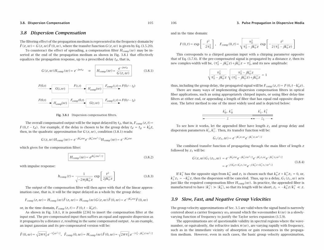
3.8 Dispersion Compensation
The filtering effect of the propagation medium is represented in the frequency domain byF(z,ω)= G(z,ω)F(0,ω), where the transfer functionG(z,ω) is given by Eq. (3.5.20).
To counteract the effect of spreading, a compensation filter Hcomp(ω) may be in-serted at the end of the propagation medium as shown in Fig. 3.8.1 that effectivelyequalizes the propagation response, up to a prescribed delay td, that is,
G(z,ω)Hcomp(ω)= e−jωtd ⇒ Hcomp(ω)= e−jωtdG(z,ω)
(3.8.1)
Fig. 3.8.1 Dispersion compensation filters.
The overall compensated output will be the input delayed by td, that is, Fcomp(z, t)=F(0, t − td). For example, if the delay is chosen to be the group delay td = tg = k′0z,then, in the quadratic approximation for G(z,ω), condition (3.8.1) reads:
G(z,ω)Hcomp(ω)= e−jk′0zωe−jk′′0 zω2/2Hcomp(ω)= e−jk′0zω
which gives for the compensation filter:
Hcomp(ω)= ejk′′0 zω2/2 (3.8.2)
with impulse response:
hcomp(t)= 1√−2πjk′′0 z
exp
[t2
2jk′′0 z
](3.8.3)
The output of the compensation filter will then agree with that of the linear approx-imation case, that is, it will be the input delayed as a whole by the group delay:
Fcomp(z,ω)= Hcomp(ω)F(z,ω)= Hcomp(ω)G(z,ω)F(0,ω)= e−jk′0zωF(0,ω)
or, in the time domain, Fcomp(z, t)= F(0, t − k′0z).As shown in Fig. 3.8.1, it is possible [236] to insert the compensation filter at the
input end. The pre-compensated input then suffers an equal and opposite dispersion asit propagates by a distance z, resulting in the same compensated output. As an example,an input gaussian and its pre-compensated version will be:
F(0,ω)=√
2πτ20 e−τ
20ω2/2, Fcomp(0,ω)= Hcomp(ω)F(0,ω)=
√2πτ2
0 e−(τ20−jk′′0 z)ω2/2
106 3. Pulse Propagation in Dispersive Media
and in the time domain:
F(0, t)= exp
[− t2
2τ20
], Fcomp(0, t)=
√√√√ τ20
τ20 − jk′′0 z
exp
[− t2
2(τ20 − jk′′0 z)
]
This corresponds to a chirped gaussian input with a chirping parameter oppositethat of Eq. (3.7.6). If the pre-compensated signal is propagated by a distance z, then itsnew complex-width will be, (τ2
0 − jk′′0 z)+jk′′0 z = τ20, and its new amplitude:
√√√√ τ20
τ20 − jk′′0 z
√√√√ τ20 − jk′′0 z
(τ20 − jk′′0 z)+jk′′0 z
= 1
thus, including the group delay, the propagated signal will be Fcomp(z, t)= F(0, t−k′0z).There are many ways of implementing dispersion compensation filters in optical
fiber applications, such as using appropriately chirped inputs, or using fiber delay-linefilters at either end, or appending a length of fiber that has equal end opposite disper-sion. The latter method is one of the most widely used and is depicted below:
To see how it works, let the appended fiber have length z1 and group delay anddispersion parameters k′1, k′′1 . Then, its transfer function will be:
G1(z1,ω)= e−jk′1z1ωe−jk′′1 z1ω2/2
The combined transfer function of propagating through the main fiber of length zfollowed by z1 will be:
G(z,ω)G1(z1,ω) = e−jk′0zωe−jk′′0 zω2/2e−jk′1z1ωe−jk
′′1 z1ω2/2
= e−j(k′0z+k′1z1)ωe−j(k′′0 z+k′′1 z1)ω2/2
(3.8.4)
If k′′1 has the opposite sign from k′′0 and z1 is chosen such that k′′0 z+ k′′1 z1 = 0, or,k′′1 z1 = −k′′0 z, then the dispersion will be canceled. Thus, up to a delay, G1(z1,ω) actsjust like the required compensation filter Hcomp(ω). In practice, the appended fiber ismanufactured to have |k′′1 | � |k′′0 |, so that its length will be short, z1 = −k′′0 z/k′′1 z.
3.9 Slow, Fast, and Negative Group Velocities
The group velocity approximations of Sec. 3.5 are valid when the signal band is narrowlycentered about a carrier frequencyω0 around which the wavenumber k(ω) is a slowly-varying function of frequency to justify the Taylor series expansion (3.5.9).
The approximations are of questionable validity in spectral regions where the wave-number, or equivalently, the refractive index n(ω), are varying rapidly with frequency,such as in the immediate vicinity of absorption or gain resonances in the propaga-tion medium. However, even in such cases, the basic group velocity approximation,
3.9. Slow, Fast, and Negative Group Velocities 107
F(z, t)= F(0, t − z/vg), can be justified provided the signal bandwidth Δω is suffi-ciently narrow and the propagation distance z is sufficiently short to minimize spread-ing and chirping; for example, in the gaussian case, this would require the condition|k′′0 z| τ2
0, or, |k′′0 z(Δω)2| 1, as well as the condition | Im(k0)z| 1 to minimizeamplitude distortions due to absorption or gain.
Because near resonances the group velocity vg can be subluminal, superluminal, ornegative, this raises the issue of how to interpret the result F(z, t)= F(0, t−z/vg). Forexample, if vg is negative within a medium of thickness z, then the group delay tg = z/vgwill be negative, corresponding to a time advance, and the envelope’s peak will appearto exit the medium before it even enters it. Indeed, experiments have demonstratedsuch apparently bizarre behavior [266,267,285]. As we mentioned in Sec. 3.2, this isnot at odds with relativistic causality because the peaks are not necessarily causallyrelated—only sharp signal fronts may not travel faster than c.
The gaussian pulses used in the above experiments do not have a sharp front. Their(infinitely long) forward tail can enter and exit the medium well before the peak does.Because of the spectral reshaping taking place due to the propagation medium’s re-sponse e−jk(ω)z, the forward portion of the pulse that is already within the propagationmedium, and the portion that has already exited, can get reshaped into a peak that ap-pears to have exited before the peak of the input has entered. In fact, before the incidentpeak enters the medium, two additional peaks develop caused by the forward tail of theinput: the one that has already exited the medium, and another one within the mediumtraveling backwards with the negative group velocity vg. Such backward-moving peakshave been observed experimentally [313]. We clarify these remarks later on by meansof the numerical example shown in Fig. 3.9.4 and elaborated further in Problem 3.10.
Next, we look at some examples that are good candidates for demonstrating theabove ideas. We recall from Sec. 1.18 the following relationships between wavenumberk = β − jα, refractive index n = nr − jni, group index ng, and dispersion coefficientk′′, where all the quantities are functions of the frequency ω:
k = β− jα = ωnc= ω(nr − jni)
c
k′ = dkdω
= 1
cd(ωn)dω
= ngc
⇒ vg = 1
Re(k′)= c
Re(ng)
k′′ = d2kdω2
= 1
cdngdω
= n′gc
(3.9.1)
We consider first a single-resonance absorption or gain Lorentz medium with per-mittivity given by Eq. (1.11.13), that is, having susceptibility χ and refractive index n:
χ = fω2p
ω2r −ω2 + jωγ ⇒ n =
√1+ χ =
√√√√1+ fω2p
ω2r −ω2 + jωγ (3.9.2)
where ωr,γ are the resonance frequency and linewidth, and ωp, f are the plasma fre-quency and oscillator strength. For an absorption medium, we will set f = 1, for a gainmedium, f = −1, and for vacuum, f = 0. To simplify the algebra, we may use the
108 3. Pulse Propagation in Dispersive Media
approximation (1.18.3), that is,
n =√
1+ χ � 1+ 1
2χ = 1+ fω2
p/2ω2r −ω2 + jωγ (3.9.3)
This approximation is fairly accurate in the numerical examples that we consider.The corresponding complex-valued group index follows from (3.9.3):
ng = d(ωn)dω
= 1+ fω2p(ω2 +ω2
r)/2(ω2
r −ω2 + jωγ)2(3.9.4)
with real and imaginary parts:
Re(ng) = 1+ fω2p(ω2 +ω2
r)[(ω2 −ω2
r)2−ω2γ2]
[(ω2 −ω2
r)2+ω2γ2]2
Im(ng) =fω2
pγω(ω4 −ω4r)[
(ω2 −ω2r)2+ω2γ2
]2
(3.9.5)
Similarly, the dispersion coefficient dng/dω is given by:
n′g =dngdω
= fω2p(ω3 + 3ω2
rω− jγω2r)
(ω2r −ω2 + jωγ)3
(3.9.6)
At resonance, ω =ωr , we find the values:
n = 1− j fω2p
2γωr, ng = 1− fω
2p
γ2(3.9.7)
For an absorption medium (f = 1), if ωp < γ, the group index will be 0 < ng < 1,resulting into a superluminal group velocity vg = c/ng > c, but if γ < ωp, which is themore typical case, then the group index will become negative, resulting into a negativevg = c/ng < 0. This is illustrated in the top row of graphs of Fig. 3.9.1. On the otherhand, for a gain medium (f = −1), the group index is always ng > 1 at resonance,resulting into a subluminal group velocity vg = c/ng < c. This is illustrated in themiddle and bottom rows of graphs of Fig. 3.9.1.
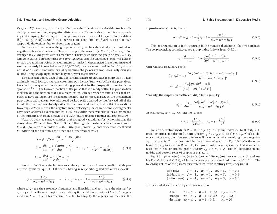
Fig. 3.9.1 plots n(ω)= nr(ω)−jni(ω) and Re[ng(ω)
]versus ω, evaluated us-
ing Eqs. (3.9.3) and (3.9.4), with the frequency axis normalized in units of ω/ωr . Thefollowing values of the parameters were used (with arbitrary frequency units):
(top row) f = +1 , ωp = 1 , ωr = 5 , γ = 0.4(middle row) f = −1 , ωp = 1 , ωr = 5 , γ = 0.4(bottom row) f = −1 , ωp = 1 , ωr = 5 , γ = 0.2
The calculated values of n,ng at resonance were:
(top) ω =ωr , n = 1− 0.25j , ng = −5.25(middle) ω =ωr , n = 1+ 0.25j , ng = 7.25(bottom) ω =ωr , n = 1+ 0.5j , ng = 26
3.9. Slow, Fast, and Negative Group Velocities 109
0.5 1 1.50.8
1
1.2
ω0
signal band
ω /ωr
real part, nr(ω)
0.5 1 1.50
0.1
0.2
0.3
0.4
0.5
ω0 ω /ωr
imaginary part, ni(ω)
0.5 1 1.5−6
0
1
3
ω0 ω /ωr
group index, Re(ng)
0.5 1 1.50.8
1
1.2
ω /ωr
real part, nr(ω)
0.5 1 1.5−0.5
−0.4
−0.3
−0.2
−0.1
0
ω /ωr
imaginary part, ni(ω)
0.5 1 1.5−1
0
1
8
ω0 ω /ωr
group index, Re(ng)
0.5 1 1.50.7
1
1.3
ω /ωr
real part, nr(ω)
0.5 1 1.5−0.5
−0.4
−0.3
−0.2
−0.1
0
ω /ωr
imaginary part, ni(ω)
0.5 1 1.5−4
01
28
ω0 ω /ωr
group index, Re(ng)
Fig. 3.9.1 Slow, fast, and negative group velocities (at off resonance).
Operating at resonance is not a good idea because of the fairly substantial amountsof attenuation or gain arising from the imaginary part ni of the refractive index, whichwould cause amplitude distortions in the signal as it propagates.
A better operating frequency band is at off resonance where the attenuation or gainare lower [272]. The top row of Fig. 3.9.1 shows such a band centered at a frequencyω0
on the right wing of the resonance, with a narrow enough bandwidth to justify the Taylorseries expansion (3.5.9). The group velocity behavior is essentially the reverse of that atresonance, that is, vg becomes subluminal for the absorption medium, and superluminalor negative for the gain medium. The carrier frequencyω0 and the calculated values ofn,ng at ω =ω0 were as follows:
(top, slow) ω0/ωr = 1.12 , n = 0.93− 0.02j , ng = 1.48+ 0.39j(middle, fast) ω0/ωr = 1.12 , n = 1.07+ 0.02j , ng = 0.52− 0.39j(bottom, negative) ω0/ωr = 1.07 , n = 1.13+ 0.04j , ng = −0.58− 1.02j
We note the sign and magnitude of Re(ng) and the substantially smaller values ofthe imaginary part ni. For the middle graph, the group index remains in the interval
110 3. Pulse Propagation in Dispersive Media
0 < Re(ng)< 1, and hence vg > c, for all values of the frequency in the right wing ofthe resonance.
In order to get negative values for Re(ng) and for vg, the linewidth γ must be re-duced. As can be seen in the bottom row of graphs, Re(ng) becomes negative over asmall range of frequencies to the right and left of the resonance. The edge frequenciescan be calculated from the zero-crossings of Re(ng) and are shown on the graph. Forthe given parameter values, they were found to be (in units of ω/ωr):
[0.9058, 0.9784] , [1.0221, 1.0928]
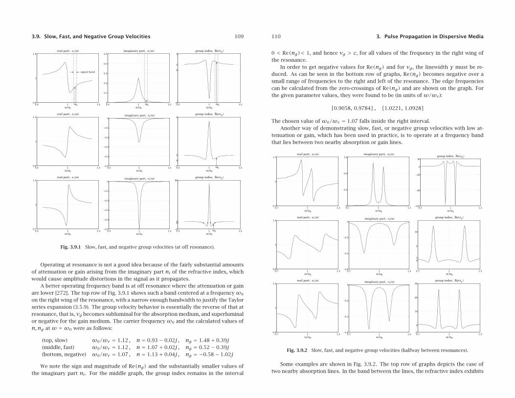
The chosen value of ω0/ωr = 1.07 falls inside the right interval.Another way of demonstrating slow, fast, or negative group velocities with low at-
tenuation or gain, which has been used in practice, is to operate at a frequency bandthat lies between two nearby absorption or gain lines.
0.7 1 1.30.3
1
1.7
ω /ω0
real part, nr(ω)
0.7 1 1.30
0.4
0.8
1.2
ω /ω0
imaginary part, ni(ω)
0.7 1 1.3−100
−60
−20
0
20
ω /ω0
group index, Re(ng)
0.7 1 1.30.6
1
1.4
ω /ω0
real part, nr(ω)
0.7 1 1.3−0.6
−0.4
−0.2
0
ω /ω0
imaginary part, ni(ω)
0.7 1 1.3
01
5
10
ω /ω0
group index, Re(ng)
0.7 1 1.30.6
1
1.4
ω /ω0
real part, nr(ω)
0.7 1 1.3−0.6
−0.4
−0.2
0
ω /ω0
imaginary part, ni(ω)
0.7 1 1.3−5
0
10
20
30
ω /ω0
group index, Re(ng)
Fig. 3.9.2 Slow, fast, and negative group velocities (halfway between resonances).
Some examples are shown in Fig. 3.9.2. The top row of graphs depicts the case oftwo nearby absorption lines. In the band between the lines, the refractive index exhibits
3.9. Slow, Fast, and Negative Group Velocities 111
normal dispersion. Exactly at midpoint, the attenuation is minimal and the real partnr has a steep slope that causes a large group index, Re(ng)� 1, and hence a smallpositive group velocity 0 < vg c. In experiments, very sharp slopes have beenachieved through the use of the so-called “electromagnetically induced transparency,”resulting into extremely slow group velocities of the order of tens of m/sec [327].
The middle row of graphs depicts two nearby gain lines [273] with a small gainat midpoint and a real part nr that has a negative slope resulting into a group index0 < Re(ng)< 1, and a superluminal group velocity vg > c.
Choosing more closely separated peaks in the third row of graphs, has the effect ofincreasing the negative slope of nr , thus causing the group index to become negativeat midpoint, Re(ng)< 0, resulting in negative group velocity, vg < 0. Experimentsdemonstrating this behavior have received a lot of attention [285].
The following expressions were used in Fig. 3.9.2 for the refractive and group indices,with f = 1 for the absorption case, and f = −1 for the gain case:
n = 1+ fω2p/2
ω21 −ω2 + jωγ +
fω2p/2
ω22 −ω2 + jωγ
ng = 1+ fω2p(ω2 +ω2
1)/2(ω2
1 −ω2 + jωγ)2+ fω2
p(ω2 +ω22)/2
(ω22 −ω2 + jωγ)2
(3.9.8)
The two peaks were symmetrically placed about the midpoint frequency ω0, thatis, at ω1 = ω0 − Δ and ω2 = ω0 + Δ, and a common linewidth γ was chosen. Theparticular numerical values used in this graph were:
(top, slow) f = +1 , ωp = 1 , ω0 = 5 , Δ = 0.25 , γ = 0.1(middle, fast) f = −1 , ωp = 1 , ω0 = 5 , Δ = 0.75 , γ = 0.3(bottom, negative) f = −1 , ωp = 1 , ω0 = 5 , Δ = 0.50 , γ = 0.2
resulting in the following values for n and ng:
(top, slow) n = 0.991− 0.077j , ng = 8.104+ 0.063j(middle, fast) n = 1.009+ 0.026j , ng = 0.208− 0.021j(bottom, negative) n = 1.009+ 0.039j , ng = −0.778− 0.032j
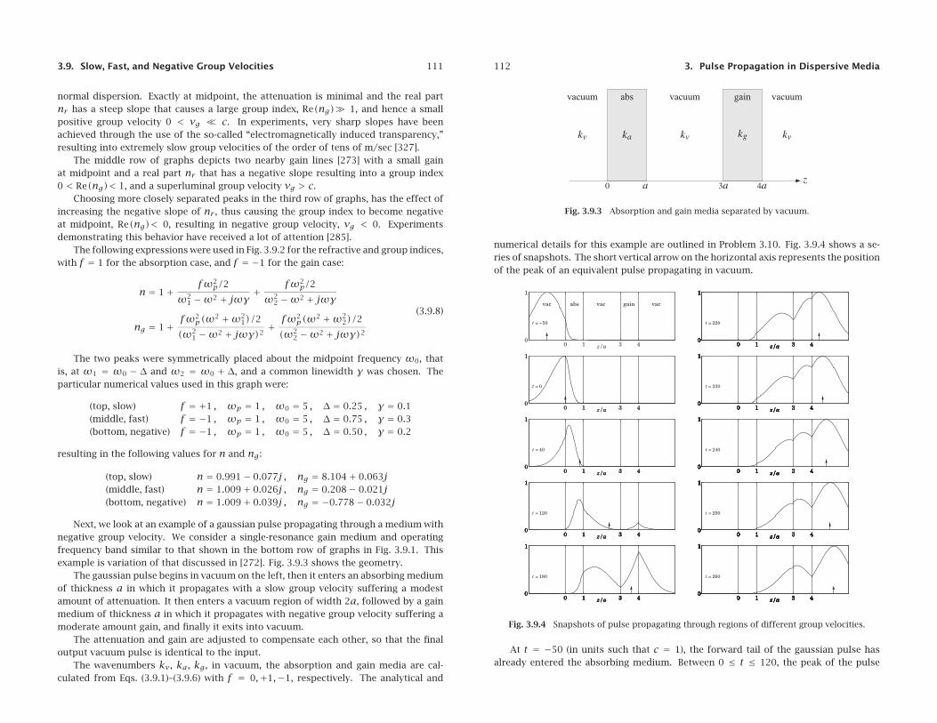
Next, we look at an example of a gaussian pulse propagating through a medium withnegative group velocity. We consider a single-resonance gain medium and operatingfrequency band similar to that shown in the bottom row of graphs in Fig. 3.9.1. Thisexample is variation of that discussed in [272]. Fig. 3.9.3 shows the geometry.
The gaussian pulse begins in vacuum on the left, then it enters an absorbing mediumof thickness a in which it propagates with a slow group velocity suffering a modestamount of attenuation. It then enters a vacuum region of width 2a, followed by a gainmedium of thickness a in which it propagates with negative group velocity suffering amoderate amount gain, and finally it exits into vacuum.
The attenuation and gain are adjusted to compensate each other, so that the finaloutput vacuum pulse is identical to the input.
The wavenumbers kv, ka, kg, in vacuum, the absorption and gain media are cal-culated from Eqs. (3.9.1)–(3.9.6) with f = 0,+1,−1, respectively. The analytical and
112 3. Pulse Propagation in Dispersive Media
Fig. 3.9.3 Absorption and gain media separated by vacuum.
numerical details for this example are outlined in Problem 3.10. Fig. 3.9.4 shows a se-ries of snapshots. The short vertical arrow on the horizontal axis represents the positionof the peak of an equivalent pulse propagating in vacuum.
0 1 3 40
1
z/a
t = −50
vac abs vac gain vac
0 1 3 40
1
z/a
t = −50
vac abs vac gain vac
0 1 3 40
1
z/a
t = 0
0 1 3 40
1
z/a
t = 40
0 1 3 40
1
z/a
t = 120
0 1 3 40
1
z/a
t = 180
0 1 3 40
1
z/a
t = 220
0 1 3 40
1
z/a
t = −50
vac abs vac gain vac
0 1 3 40
1
z/a
t = 0
0 1 3 40
1
z/a
t = −50
vac abs vac gain vac
0 1 3 40
1
z/a
t = 0
0 1 3 40
1
z/a
t = 40
0 1 3 40
1
z/a
t = 120
0 1 3 40
1
z/a
t = 180
0 1 3 40
1
z/a
t = 220
0 1 3 40
1
z/a
t = 230
0 1 3 40
1
z/a
t = −50
vac abs vac gain vac
0 1 3 40
1
z/a
t = 0
0 1 3 40
1
z/a
t = 40
0 1 3 40
1
z/a
t = −50
vac abs vac gain vac
0 1 3 40
1
z/a
t = 0
0 1 3 40
1
z/a
t = 40
0 1 3 40
1
z/a
t = 120
0 1 3 40
1
z/a
t = 180
0 1 3 40
1
z/a
t = 220
0 1 3 40
1
z/a
t = 230
0 1 3 40
1
z/a
t = 240
0 1 3 40
1
z/a
t = −50
vac abs vac gain vac
0 1 3 40
1
z/a
t = 0
0 1 3 40
1
z/a
t = 40
0 1 3 40
1
z/a
t = 120
0 1 3 40
1
z/a
t = −50
vac abs vac gain vac
0 1 3 40
1
z/a
t = 0
0 1 3 40
1
z/a
t = 40
0 1 3 40
1
z/a
t = 120
0 1 3 40
1
z/a
t = 180
0 1 3 40
1
z/a
t = 220
0 1 3 40
1
z/a
t = 230
0 1 3 40
1
z/a
t = 240
0 1 3 40
1
z/a
t = 250
0 1 3 40
1
z/a
t = −50
vac abs vac gain vac
0 1 3 40
1
z/a
t = 0
0 1 3 40
1
z/a
t = 40
0 1 3 40
1
z/a
t = 120
0 1 3 40
1
z/a
t = 180
0 1 3 40
1
z/a
t = −50
vac abs vac gain vac
0 1 3 40
1
z/a
t = 0
0 1 3 40
1
z/a
t = 40
0 1 3 40
1
z/a
t = 120
0 1 3 40
1
z/a
t = 180
0 1 3 40
1
z/a
t = 220
0 1 3 40
1
z/a
t = 230
0 1 3 40
1
z/a
t = 240
0 1 3 40
1
z/a
t = 250
0 1 3 40
1
z/a
t = 260
Fig. 3.9.4 Snapshots of pulse propagating through regions of different group velocities.
At t = −50 (in units such that c = 1), the forward tail of the gaussian pulse hasalready entered the absorbing medium. Between 0 ≤ t ≤ 120, the peak of the pulse
3.10. Chirp Radar and Pulse Compression 113
has entered the absorbing medium and is being attenuated as it propagates while it lagsbehind the equivalent vacuum pulse because vg < c.
At t = 120, while the peak is still in the absorbing medium, the forward tail haspassed through the middle vacuum region and has already entered into the gain mediumwhere it begins to get amplified. At t = 180, the peak has moved into the middle vacuumregion, but the forward tail has been sufficiently amplified by the gain medium and isbeginning to form a peak whose tail has already exited into the rightmost vacuum region.
At t = 220, the peak is still within the middle vacuum region, but the output peakhas already exited into the right, while another peak has formed at the right side of thegain medium and begins to move backwards with the negative group velocity, vg < 0.Meanwhile, the output peak has caught up with the equivalent vacuum peak.
Between 230 ≤ t ≤ 260, the peak within the gain medium continues to move back-wards while the output vacuum peak moves to the right. As we mentioned earlier, suchoutput peaks that have exited before the input peaks have entered the gain medium,including the backward moving peaks, have been observed experimentally [313].
A MATLAB movie of this example may be seen by running the file grvmovie1.m in themovies subdirectory of the ewa toolbox. See also the movie grvmovie2.m in which thecarrier frequency has been increased and corresponds to a superluminal group velocity(vg > c) for the gain medium. In this case, which is also described in Problem 3.10, allthe peaks are moving forward.
3.10 Chirp Radar and Pulse Compression
Pulse Radar Requirements
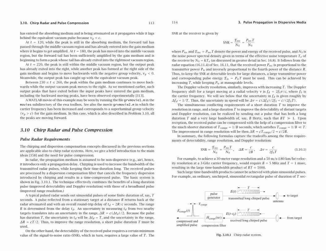
The chirping and dispersion compensation concepts discussed in the previous sectionsare applicable also to chirp radar systems. Here, we give a brief introduction to the mainideas [358] and the need for pulse compression.
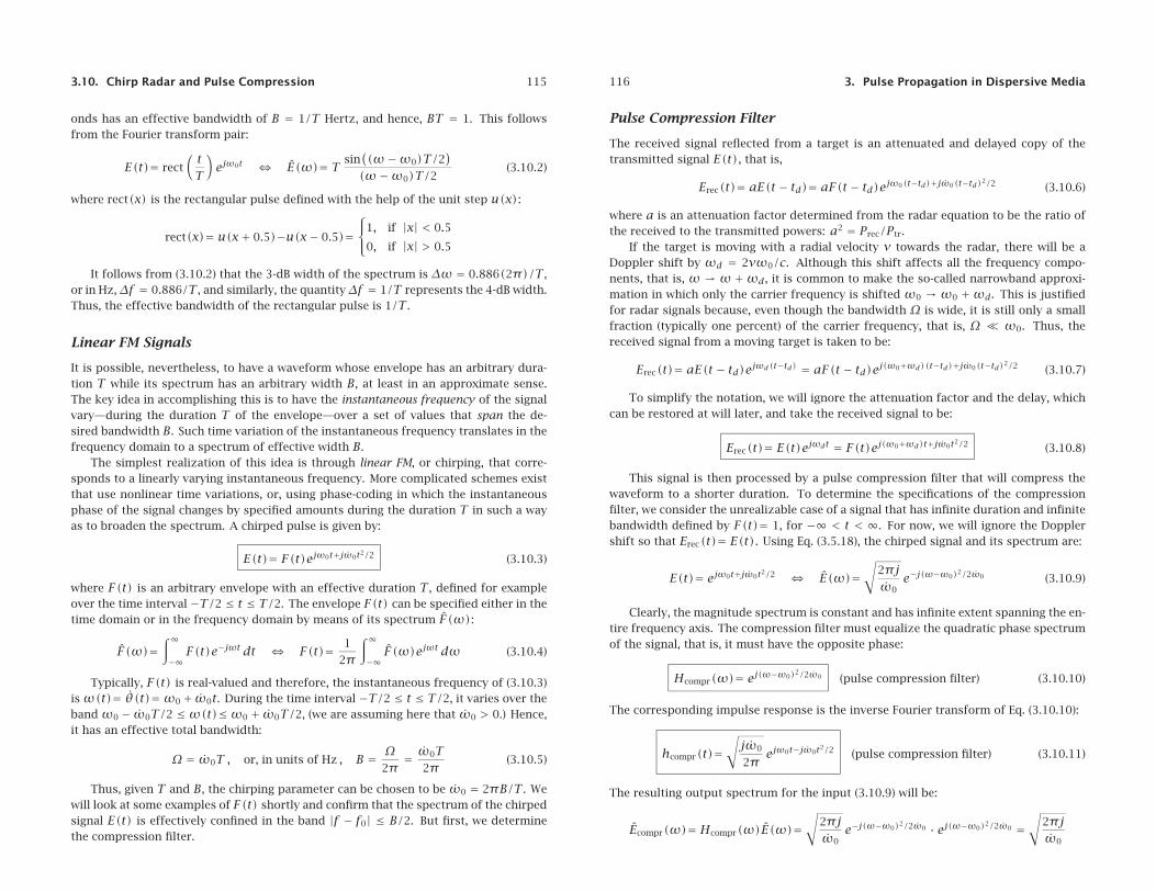
In radar, the propagation medium is assumed to be non-dispersive (e.g., air), hence,it introduces only a propagation delay. Chirping is used to increase the bandwidth of thetransmitted radar pulses, while keeping their time-duration long. The received pulsesare processed by a dispersion compensation filter that cancels the frequency dispersionintroduced by chirping and results in a time-compressed pulse. The basic system isshown in Fig. 3.10.1. The technique effectively combines the benefits of a long-durationpulse (improved detectability and Doppler resolution) with those of a broadband pulse(improved range resolution.)
A typical pulsed radar sends out sinusoidal pulses of some finite duration of, say, Tseconds. A pulse reflected from a stationary target at a distance R returns back at theradar attenuated and with an overall round-trip delay of td = 2R/c seconds. The rangeR is determined from the delay td. An uncertainty in measuring td from two nearbytargets translates into an uncertainty in the range, ΔR = c(Δtd)/2. Because the pulsehas duration T, the uncertainty in td will be Δtd = T, and the uncertainty in the range,ΔR = cT/2. Thus, to improve the range resolution, a short pulse duration T must beused.
On the other hand, the detectability of the received pulse requires a certain minimumvalue of the signal-to-noise ratio (SNR), which in turn, requires a large value of T. The
114 3. Pulse Propagation in Dispersive Media
SNR at the receiver is given by
SNR = Erec
N0= PrecT
N0
wherePrec andErec = PrecT denote the power and energy of the received pulse, andN0 isthe noise power spectral density given in terms of the effective noise temperature Te ofthe receiver byN0 = kTe (as discussed in greater detail in Sec. 16.8). It follows from theradar equation (16.11.4) of Sec. 16.11, that the received power Prec is proportional to thetransmitter power Ptr and inversely proportional to the fourth power of the distance R.Thus, to keep the SNR at detectable levels for large distances, a large transmitter powerand corresponding pulse energy Etr = PtrT must be used. This can be achieved byincreasing T, while keeping Ptr at manageable levels.
The Doppler velocity resolution, similarly, improves with increasing T. The Dopplerfrequency shift for a target moving at a radial velocity v is fd = 2f0v/c, where f0 isthe carrier frequency. We will see below that the uncertainty in fd is given roughly byΔfd = 1/T. Thus, the uncertainty in speed will be Δv = c(Δfd)/2f0 = c/(2f0T).
The simultaneous conflicting requirements of a short duration T to improve theresolution in range, and a large durationT to improve the detectability of distant targetsand Doppler resolution, can be realized by sending out a pulse that has both a longduration T and a very large bandwidth of, say, B Hertz, such that BT � 1. Uponreception, the received pulse can be compressed with the help of a compression filter tothe much shorter duration of Tcompr = 1/B seconds, which satisfies Tcompr = 1/B T.The improvement in range resolution will be then ΔR = cTcompr/2 = c/2B.
In summary, the following formulas capture the tradeoffs among the three require-ments of detectability, range resolution, and Doppler resolution:
SNR = Erec
N0= PrecT
N0, ΔR = c
2B, Δv = c
2f0T(3.10.1)
For example, to achieve a 30-meter range resolution and a 50 m/s (180 km/hr) veloc-ity resolution at a 3-GHz carrier frequency, would require B = 5 MHz and T = 1 msec,resulting in the large time-bandwidth product of BT = 5000.
Such large time-bandwidth products cannot be achieved with plain sinusoidal pulses.For example, an ordinary, unchirped, sinusoidal rectangular pulse of duration of T sec-
Fig. 3.10.1 Chirp radar system.
3.10. Chirp Radar and Pulse Compression 115
onds has an effective bandwidth of B = 1/T Hertz, and hence, BT = 1. This followsfrom the Fourier transform pair:
E(t)= rect(tT
)ejω0t � E(ω)= T sin
((ω−ω0)T/2
)(ω−ω0)T/2
(3.10.2)
where rect(x) is the rectangular pulse defined with the help of the unit step u(x):
rect(x)= u(x+ 0.5)−u(x− 0.5)=⎧⎨⎩1, if |x| < 0.5
0, if |x| > 0.5
It follows from (3.10.2) that the 3-dB width of the spectrum is Δω = 0.886(2π)/T,or in Hz,Δf = 0.886/T, and similarly, the quantityΔf = 1/T represents the 4-dB width.Thus, the effective bandwidth of the rectangular pulse is 1/T.
Linear FM Signals
It is possible, nevertheless, to have a waveform whose envelope has an arbitrary dura-tion T while its spectrum has an arbitrary width B, at least in an approximate sense.The key idea in accomplishing this is to have the instantaneous frequency of the signalvary—during the duration T of the envelope—over a set of values that span the de-sired bandwidth B. Such time variation of the instantaneous frequency translates in thefrequency domain to a spectrum of effective width B.
The simplest realization of this idea is through linear FM, or chirping, that corre-sponds to a linearly varying instantaneous frequency. More complicated schemes existthat use nonlinear time variations, or, using phase-coding in which the instantaneousphase of the signal changes by specified amounts during the duration T in such a wayas to broaden the spectrum. A chirped pulse is given by:
E(t)= F(t)ejω0t+jω0t2/2 (3.10.3)
where F(t) is an arbitrary envelope with an effective duration T, defined for exampleover the time interval −T/2 ≤ t ≤ T/2. The envelope F(t) can be specified either in thetime domain or in the frequency domain by means of its spectrum F(ω):
F(ω)=∫∞−∞F(t)e−jωt dt � F(t)= 1
2π
∫∞−∞F(ω)ejωt dω (3.10.4)
Typically, F(t) is real-valued and therefore, the instantaneous frequency of (3.10.3)isω(t)= θ(t)=ω0+ ω0t. During the time interval −T/2 ≤ t ≤ T/2, it varies over theband ω0 − ω0T/2 ≤ω(t)≤ω0 + ω0T/2, (we are assuming here that ω0 > 0.) Hence,it has an effective total bandwidth:
Ω = ω0T , or, in units of Hz , B = Ω2π
= ω0T2π
(3.10.5)
Thus, given T and B, the chirping parameter can be chosen to be ω0 = 2πB/T. Wewill look at some examples of F(t) shortly and confirm that the spectrum of the chirpedsignal E(t) is effectively confined in the band |f − f0| ≤ B/2. But first, we determinethe compression filter.
116 3. Pulse Propagation in Dispersive Media
Pulse Compression Filter
The received signal reflected from a target is an attenuated and delayed copy of thetransmitted signal E(t), that is,
Erec(t)= aE(t − td)= aF(t − td)ejω0(t−td)+jω0(t−td)2/2 (3.10.6)
where a is an attenuation factor determined from the radar equation to be the ratio ofthe received to the transmitted powers: a2 = Prec/Ptr.
If the target is moving with a radial velocity v towards the radar, there will be aDoppler shift by ωd = 2vω0/c. Although this shift affects all the frequency compo-nents, that is, ω → ω +ωd, it is common to make the so-called narrowband approxi-mation in which only the carrier frequency is shifted ω0 → ω0 +ωd. This is justifiedfor radar signals because, even though the bandwidth Ω is wide, it is still only a smallfraction (typically one percent) of the carrier frequency, that is, Ω ω0. Thus, thereceived signal from a moving target is taken to be:
Erec(t)= aE(t − td)ejωd(t−td) = aF(t − td)ej(ω0+ωd)(t−td)+jω0(t−td)2/2 (3.10.7)
To simplify the notation, we will ignore the attenuation factor and the delay, whichcan be restored at will later, and take the received signal to be:
Erec(t)= E(t)ejωdt = F(t)ej(ω0+ωd)t+jω0t2/2 (3.10.8)
This signal is then processed by a pulse compression filter that will compress thewaveform to a shorter duration. To determine the specifications of the compressionfilter, we consider the unrealizable case of a signal that has infinite duration and infinitebandwidth defined by F(t)= 1, for −∞ < t < ∞. For now, we will ignore the Dopplershift so that Erec(t)= E(t). Using Eq. (3.5.18), the chirped signal and its spectrum are:
E(t)= ejω0t+jω0t2/2 � E(ω)=√
2πjω0
e−j(ω−ω0)2/2ω0 (3.10.9)
Clearly, the magnitude spectrum is constant and has infinite extent spanning the en-tire frequency axis. The compression filter must equalize the quadratic phase spectrumof the signal, that is, it must have the opposite phase:
Hcompr(ω)= ej(ω−ω0)2/2ω0 (pulse compression filter) (3.10.10)
The corresponding impulse response is the inverse Fourier transform of Eq. (3.10.10):
hcompr(t)=√jω0
2πejω0t−jω0t2/2 (pulse compression filter) (3.10.11)
The resulting output spectrum for the input (3.10.9) will be:
Ecompr(ω)= Hcompr(ω)E(ω)=√
2πjω0
e−j(ω−ω0)2/2ω0 · ej(ω−ω0)2/2ω0 =√
2πjω0
3.10. Chirp Radar and Pulse Compression 117
that is, a constant for all ω. Hence, the input signal gets compressed into a Dirac delta:
Ecompr(t)=√
2πjω0
δ(t) (3.10.12)
When the envelope F(t) is a finite-duration signal, the resulting spectrum of thechirped signal E(t) still retains the essential quadratic phase of Eq. (3.10.9), and there-fore, the compression filter will still be given by Eq. (3.10.10) for all choices ofF(t). Usingthe stationary-phase approximation, Problem 3.17 shows that the quadratic phase is ageneral property. The group delay of this filter is given by Eq. (3.2.1):
tg = − ddω
[(ω−ω0)2
2ω0
]= −ω−ω0
ω0= −2π(f − f0)
2πB/T= −T f − f0
B
As the frequency (f − f0) increases from −B/2 to B/2, the group delay decreasesfrom T/2 to −T/2, that is, the lower frequency components, which occur earlier in thechirped pulse, suffer a longer delay through the filter. Similarly, the high frequencycomponents, which occur later in the pulse, suffer a shorter delay, the overall effectbeing the time compression of the pulse.
It is useful to demodulate the sinusoidal carrier ejω0t and writehcompr(t)= ejωotg(t)andHcompr(ω)= G(ω−ω0), where the demodulated “baseband” filter, which is knownas a quadrature-phase filter, is defined by:
g(t)=√jω0
2πe−jω0t2/2 , G(ω)= ejω2/2ω0 (quadratic phase filter) (3.10.13)
For an arbitrary envelope F(t), one can derive the following fundamental result thatrelates the output of the compression filter (3.10.11) to the Fourier transform, F(ω), ofthe envelope, when the input is E(t)= F(t)ejω0t+jω0t2/2 :
Ecompr(t)=√jω0
2πejω0t−jω0t2/2 F(−ω0t) (3.10.14)
This result belongs to a family of so-called “chirp transforms” or “Fresnel trans-forms” that find application in optics, the diffraction effects of lenses [1431], and inother areas of signal processing, such as for example, the “chirp z-transform” [48]. Toshow Eq. (3.10.14), we use the convolutional definition for the filter output:
Ecompr(t) =∫∞−∞hcompr(t − t′)E(t′)dt′
=√jω0
2π
∫∞−∞ejω0(t−t′)−jω0(t−t′)2/2 F(t′)ejω0t′+jω0t′2/2 dt′
=√jω0
2πejω0t−jω0t2/2
∫∞−∞F(t′)ej(ω0t)t′ dt′
118 3. Pulse Propagation in Dispersive Media
where the last integral factor is recognized as F(−ω0t). As an example, Eq. (3.10.12)can be derived immediately by noting that F(t)= 1 has the Fourier transform F(ω)=2πδ(ω), and therefore, using Eq. (3.10.14), we have:
Ecompr(t)=√jω0
2πejω0t−jω0t2/2 2πδ(−ω0t)=
√2πjω0
δ(t)
where we used the property δ(−ω0t)= δ(ω0t)= δ(t)/ω0 and set t = 0 in the expo-nentials.
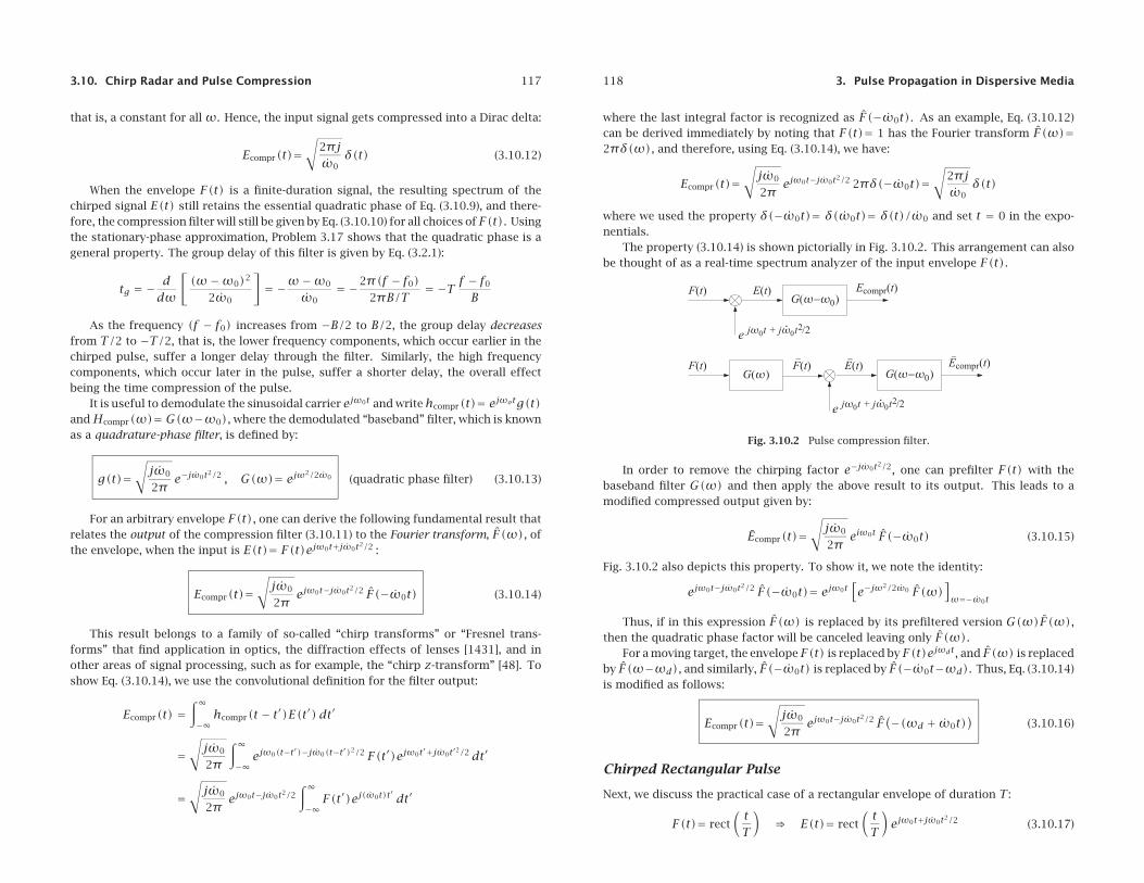
The property (3.10.14) is shown pictorially in Fig. 3.10.2. This arrangement can alsobe thought of as a real-time spectrum analyzer of the input envelope F(t).
Fig. 3.10.2 Pulse compression filter.
In order to remove the chirping factor e−jω0t2/2, one can prefilter F(t) with thebaseband filter G(ω) and then apply the above result to its output. This leads to amodified compressed output given by:
Ecompr(t)=√jω0
2πeiω0t F(−ω0t) (3.10.15)
Fig. 3.10.2 also depicts this property. To show it, we note the identity:
ejω0t−jω0t2/2 F(−ω0t)= ejω0t[e−jω
2/2ω0 F(ω)]ω=−ω0t
Thus, if in this expression F(ω) is replaced by its prefiltered version G(ω)F(ω),then the quadratic phase factor will be canceled leaving only F(ω).
For a moving target, the envelopeF(t) is replaced byF(t)ejωdt, and F(ω) is replacedby F(ω−ωd), and similarly, F(−ω0t) is replaced by F(−ω0t−ωd). Thus, Eq. (3.10.14)is modified as follows:
Ecompr(t)=√jω0
2πejω0t−jω0t2/2 F
(−(ωd + ω0t))
(3.10.16)
Chirped Rectangular Pulse
Next, we discuss the practical case of a rectangular envelope of duration T:
F(t)= rect(tT
)⇒ E(t)= rect
(tT
)ejω0t+jω0t2/2 (3.10.17)
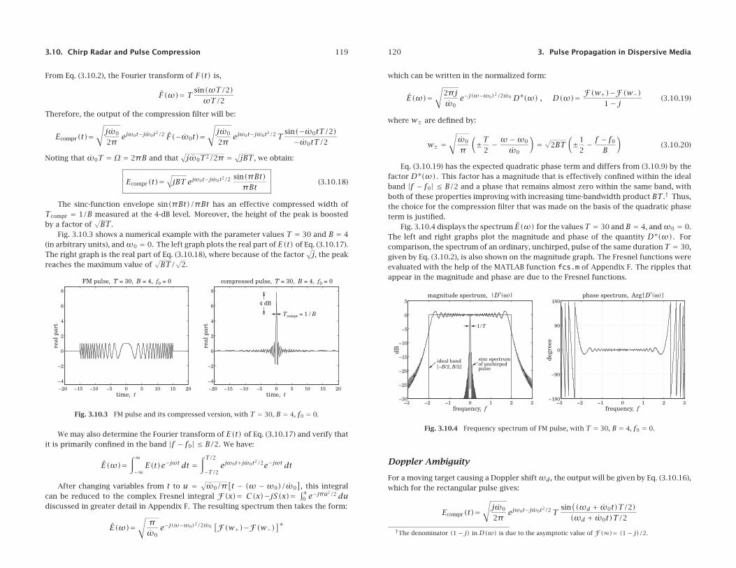
3.10. Chirp Radar and Pulse Compression 119
From Eq. (3.10.2), the Fourier transform of F(t) is,
F(ω)= T sin(ωT/2)ωT/2
Therefore, the output of the compression filter will be:
Ecompr(t)=√jω0
2πejω0t−jω0t2/2 F(−ω0t)=
√jω0
2πejω0t−jω0t2/2T
sin(−ω0tT/2)−ω0tT/2
Noting that ω0T = Ω = 2πB and that√jω0T2/2π = √
jBT, we obtain:
Ecompr(t)=√jBT ejω0t−jω0t2/2 sin(πBt)
πBt(3.10.18)
The sinc-function envelope sin(πBt)/πBt has an effective compressed width ofTcompr = 1/B measured at the 4-dB level. Moreover, the height of the peak is boostedby a factor of
√BT.
Fig. 3.10.3 shows a numerical example with the parameter values T = 30 and B = 4(in arbitrary units), andω0 = 0. The left graph plots the real part of E(t) of Eq. (3.10.17).The right graph is the real part of Eq. (3.10.18), where because of the factor
√j, the peak
reaches the maximum value of√BT/
√2.
−20 −15 −10 −5 0 5 10 15 20−4
−2
0
2
4
6
8
time, t
real
par
t
FM pulse, T = 30, B = 4, f0 = 0
−20 −15 −10 −5 0 5 10 15 20−4
−2
0
2
4
6
8
time, t
real
par
t
compressed pulse, T = 30, B = 4, f0 = 0
Tcompr = 1 / B
4 dB
Fig. 3.10.3 FM pulse and its compressed version, with T = 30, B = 4, f0 = 0.
We may also determine the Fourier transform of E(t) of Eq. (3.10.17) and verify thatit is primarily confined in the band |f − f0| ≤ B/2. We have:
E(ω)=∫∞−∞E(t)e−jωt dt =
∫ T/2−T/2
ejω0t+jω0t2/2e−jωt dt
After changing variables from t to u = √ω0/π
[t − (ω −ω0)/ω0
], this integral
can be reduced to the complex Fresnel integral F(x)= C(x)−jS(x)= ∫ x0 e−jπu
2/2 dudiscussed in greater detail in Appendix F. The resulting spectrum then takes the form:
E(ω)=√πω0
e−j(ω−ω0)2/2ω0[F(w+)−F(w−)]∗
120 3. Pulse Propagation in Dispersive Media
which can be written in the normalized form:
E(ω)=√
2πjω0
e−j(ω−ω0)2/2ω0 D∗(ω) , D(ω)= F(w+)−F(w−)1− j (3.10.19)
where w± are defined by:
w± =√ω0
π
(±T
2− ω−ω0
ω0
)= √2BT
(±1
2− f − f0
B
)(3.10.20)
Eq. (3.10.19) has the expected quadratic phase term and differs from (3.10.9) by thefactor D∗(ω). This factor has a magnitude that is effectively confined within the idealband |f − f0| ≤ B/2 and a phase that remains almost zero within the same band, withboth of these properties improving with increasing time-bandwidth product BT.† Thus,the choice for the compression filter that was made on the basis of the quadratic phaseterm is justified.
Fig. 3.10.4 displays the spectrum E(ω) for the valuesT = 30 andB = 4, andω0 = 0.The left and right graphs plot the magnitude and phase of the quantity D∗(ω). Forcomparison, the spectrum of an ordinary, unchirped, pulse of the same durationT = 30,given by Eq. (3.10.2), is also shown on the magnitude graph. The Fresnel functions wereevaluated with the help of the MATLAB function fcs.m of Appendix F. The ripples thatappear in the magnitude and phase are due to the Fresnel functions.
−3 −2 −1 0 1 2 3−30
−25
−20
−15
−10
−5
0
5
frequency, f
dB
magnitude spectrum, |D*(ω)|
sinc spectrumof unchirpedpulse
ideal band[−B/2, B/2]
1 /T
−3 −2 −1 0 1 2 3−180
−90
0
90
180
frequency, f
degr
ees
phase spectrum, Arg[D*(ω) ]
Fig. 3.10.4 Frequency spectrum of FM pulse, with T = 30, B = 4, f0 = 0.
Doppler Ambiguity
For a moving target causing a Doppler shiftωd, the output will be given by Eq. (3.10.16),which for the rectangular pulse gives:
Ecompr(t)=√jω0
2πejω0t−jω0t2/2T
sin((ωd + ω0t)T/2)(ωd + ω0t)T/2
†The denominator (1− j) in D(ω) is due to the asymptotic value of F(∞)= (1− j)/2.
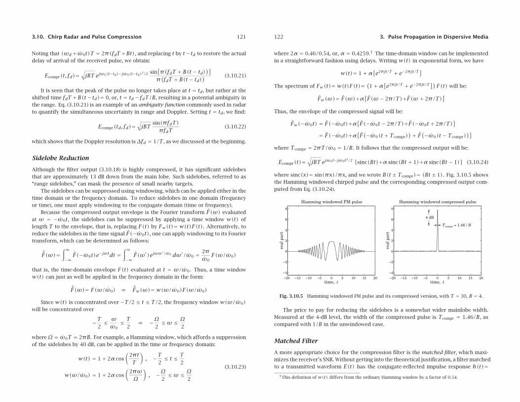
3.10. Chirp Radar and Pulse Compression 121
Noting that (ωd+ω0t)T = 2π(fdT+Bt), and replacing t by t− td to restore the actualdelay of arrival of the received pulse, we obtain:
Ecompr(t, fd)=√jBT ejω0(t−td)−jω0(t−td)2/2 sin
[π(fdT + B(t − td)
)]π(fdT + B(t − td)
) (3.10.21)
It is seen that the peak of the pulse no longer takes place at t = td, but rather at theshifted time fdT+B(t− td)= 0, or, t = td− fdT/B, resulting in a potential ambiguity inthe range. Eq. (3.10.21) is an example of an ambiguity function commonly used in radarto quantify the simultaneous uncertainty in range and Doppler. Setting t = td, we find:
Ecompr(td, fd)=√jBT
sin(πfdT)πfdT
(3.10.22)
which shows that the Doppler resolution isΔfd = 1/T, as we discussed at the beginning.
Sidelobe Reduction
Although the filter output (3.10.18) is highly compressed, it has significant sidelobesthat are approximately 13 dB down from the main lobe. Such sidelobes, referred to as“range sidelobes,” can mask the presence of small nearby targets.
The sidelobes can be suppressed using windowing, which can be applied either in thetime domain or the frequency domain. To reduce sidelobes in one domain (frequencyor time), one must apply windowing to the conjugate domain (time or frequency).
Because the compressed output envelope is the Fourier transform F(ω) evaluatedat ω = −ω0t, the sidelobes can be suppressed by applying a time window w(t) oflength T to the envelope, that is, replacing F(t) by Fw(t)= w(t)F(t). Alternatively, toreduce the sidelobes in the time signal F(−ω0t), one can apply windowing to its Fouriertransform, which can be determined as follows:
ˆF(ω)=∫∞−∞F(−ω0t)e−jωtdt =
∫∞−∞F(ω′)ejωω
′/ω0 dω′/ω0 = 2πω0
F(ω/ω0)
that is, the time-domain envelope F(t) evaluated at t = ω/ω0. Thus, a time windoww(t) can just as well be applied in the frequency domain in the form:
ˆF(ω)= F(ω/ω0) ⇒ ˆFw(ω)= w(ω/ω0)F(ω/ω0)
Since w(t) is concentrated over −T/2 ≤ t ≤ T/2, the frequency window w(ω/ω0)will be concentrated over
−T2≤ ωω0
≤ T2
⇒ −Ω2≤ω ≤ Ω
2
whereΩ = ω0T = 2πB. For example, a Hamming window, which affords a suppressionof the sidelobes by 40 dB, can be applied in the time or frequency domain:
w(t) = 1+ 2α cos(
2πtT
), −T
2≤ t ≤ T
2
w(ω/ω0) = 1+ 2α cos(
2πωΩ
), −Ω
2≤ω ≤ Ω
2
(3.10.23)
122 3. Pulse Propagation in Dispersive Media
where 2α = 0.46/0.54, or, α = 0.4259.† The time-domain window can be implementedin a straightforward fashion using delays. Writing w(t) in exponential form, we have
w(t)= 1+α[e2πjt/T + e−2πjt/T]The spectrum of Fw(t)= w(t)F(t)=
(1+α[e2πjt/T + e−2πjt/T])F(t) will be:
Fw(ω)= F(ω)+α[F(ω− 2π/T)+F(ω+ 2π/T)
]Thus, the envelope of the compressed signal will be:
Fw(−ω0t) = F(−ω0t)+α[F(−ω0t − 2π/T)+F(−ω0t + 2π/T)
]= F(−ω0t)+α
[F(−ω0(t +Tcompr)
)+ F(−ω0(t −Tcompr))]
where Tcompr = 2πT/ω0 = 1/B. It follows that the compressed output will be:
Ecompr(t)=√jBT ejω0t−jω0t2/2 [sinc(Bt)+α sinc(Bt + 1)+α sinc(Bt − 1)] (3.10.24)
where sinc(x)= sin(πx)/πx, and we wrote B(t±Tcompr)= (Bt± 1). Fig. 3.10.5 showsthe Hamming windowed chirped pulse and the corresponding compressed output com-puted from Eq. (3.10.24).
−20 −15 −10 −5 0 5 10 15 20−4
−2
0
2
4
6
8
time, tre
al p
art
Hamming windowed FM pulse
−20 −15 −10 −5 0 5 10 15 20−4
−2
0
2
4
6
8
time, t
real
par
t
Hamming windowed compressed pulse
Tcompr = 1.46 / B
4 dB
Fig. 3.10.5 Hamming windowed FM pulse and its compressed version, with T = 30, B = 4.
The price to pay for reducing the sidelobes is a somewhat wider mainlobe width.Measured at the 4-dB level, the width of the compressed pulse is Tcompr = 1.46/B, ascompared with 1/B in the unwindowed case.
Matched Filter
A more appropriate choice for the compression filter is the matched filter, which maxi-mizes the receiver’s SNR. Without getting into the theoretical justification, a filter matchedto a transmitted waveform E(t) has the conjugate-reflected impulse response h(t)=†This definition of w(t) differs from the ordinary Hamming window by a factor of 0.54.
3.11. Further Reading 123
E∗(−t) and corresponding frequency response H(ω)= E∗(ω). In particular for therectangular chirped pulse, we have:
E(t)= rect(tT
)ejω0t+jω0t2/2 ⇒ h(t)= E∗(−t)= rect
(tT
)ejω0t−jω0t2/2 (3.10.25)
which differs from our simplified compression filter by the factor rect(t/T). Its fre-quency response is given by the conjugate of Eq. (3.10.19)
H(ω)=√−2πjω0
ej(ω−ω0)2/2ω0 D(ω) , D(ω)= F(w+)−F(w−)1− j (3.10.26)
We have seen that the factor D(ω) is essentially unity within the band |f − f0| ≤B/2. Thus again, the matched filter resembles the filter (3.10.10) within this band. Theresulting output of the matched filter is remarkably similar to that of Eq. (3.10.18):
Ecompr(t)= ejω0t Tsin(πB|t| −πBt2/T)
πB|t| , for −T ≤ t ≤ T (3.10.27)
while it vanishes for |t| > T.In practice, the matched/compression filters are conveniently realized either dig-
itally using digital signal processing (DSP) techniques or using surface acoustic wave(SAW) devices [383]. Similarly, the waveform generator of the chirped pulse may berealized using DSP or SAW methods. A convenient generation method is to send animpulse (or, a broadband pulse) to the input of a filter that has as frequency responseH(ω)= E(ω), so that the impulse response of the filter is the signal E(t) that we wishto generate.
Signal design in radar is a subject in itself and the present discussion was only meantto be an introduction motivated by the similarity to dispersion compensation.
3.11 Further Reading
The topics discussed in this chapter are vast and diverse. The few references givenbelow are inevitably incomplete.
References [168–191] discuss the relationship between group velocity and energy ve-locity for lossless or lossy media, as well as the issue of electromagnetic field momentumand radiation pressure.
Some references on pulse propagation, spreading, chirping, and dispersion compen-sation in optical fibers, plasmas, and other media are [192–244], while precursors arediscussed in Sommerfeld [1287], Brillouin [192], and [245–257].
Some theoretical and experimental references on fast and negative group velocityare [258–313]. Circuit realizations of negative group delays are discussed in [314–318].References [319–350] discuss slow light and electromagnetically induced transparencyand related experiments.
Some references on chirp radar and pulse compression are [351–390]. These includephase-coding methods, as well as alternative phase modulation methods for Doppler-resistant applications.
124 3. Pulse Propagation in Dispersive Media
3.12 Problems
3.1 Using the definitions (3.2.5), show that the group and phase velocities are related by:
vg = vp + β dvpdβ
3.2 It was mentioned earlier that when vg > c, the peak of a pulse shifts forward in time asit propagates. With reference to Fig. 3.2.2, let tpeak be the time of the peak of the initialpulse E(0, t). First, show that the peak of the propagated pulse E(z, t) occurs at timetprop = tpeak+z/vg. Then, show that the peak value E(z, tprop) does not depend on the initialpeak E(0, tpeak) but rather it depends causally on the values E(0, t), for t0 ≤ t ≤ tpeak −Δt,where Δt = z/c − z/vg, which is positive if vg > c. What happens if 0 < vg < c and ifvg < 0?
3.3 Consider case 6 of the exactly solvable examples of Sec. 3.3 describing a lossy transmissionline with distributed parameters L′, C′, R′, G′. The voltage and current along the line satisfythe so-called telegrapher’s equations:
∂V∂z
+ L′ ∂I∂t+R′I = 0 ,
∂I∂z
+C′ ∂V∂t
+G′V = 0 (3.12.1)
The voltage impulse response V(z, t) of the line is given by Eq. (3.3.1), where tf = z/c,a+ b = R′/L′, a− b = G′/C′, and c = 1/
√L′C′:
V(z, t)= δ(t − tf )e−atf + e−atI1(b√t2 − t2f
)√t2 − t2f
btf u(t − tf )
Show that the corresponding current I(z, t) is given by
√L′
C′I(z, t)= δ(t − tf )e−atf + e−at
⎡⎣ I1
(b√t2 − t2f
)√t2 − t2f
bt − bI0(b√t2 − t2f
)⎤⎦u(t − tf )
by verifying that V and I satisfy Eqs. (3.12.1). Hint: Use the relationships: I′0(x)= I1(x) andI′1(x)= I0(x)−I1(x)/x between the Bessel functions I0(x) and I1(x).Next, show that the Fourier transforms of V(z, t) and I(z, t) are:
V(z,ω)= e−γz , I(z,ω)= e−γz
Z
where γ,Z are the propagation constant and characteristic impedance (see Sec. 11.6):
γ = jk =√R′ + jωL′
√G′ + jωC′ , Z =
√R′ + jωL′G′ + jωC′
3.4 Computer Experiment—Transient Behavior. Reproduce the results and graphs of the Figures3.4.1, 3.4.2, and 3.4.3.
3.5 Consider the propagated envelope of a pulse under the linear approximation of Eq. (3.5.13),that is, F(z, t)= F(0, t−k′0z), for the case of a complex-valued wavenumber, k′0 = β′0− jα′0.For a gaussian envelope:
F(z, t)= F(0, t − k′0z)= exp
[−(t − (β′0 − jα′0)z
)2
2τ20
]
3.12. Problems 125
Determine an expression for its magnitude |F(z, t)|. Then show that the maximum of|F(z, t)| with respect to t at a given fixed z is moving with the group velocity vg = 1/β′0.
Alternatively, at fixed t show that the maximum with respect to z of the snapshot |F(z, t)|is moving with velocity [198]:
v = β′0β′20 −α′20
3.6 Consider the propagating wave E(z, t)= F(z, t)ejω0t−jk0z. Assuming the quadratic approx-imation (3.5.9), show that the envelope F(z, t) satisfies the partial differential equation:
(∂∂z
+ k′0∂∂t− j k
′′0
2
∂2
∂t2
)F(z, t)= 0
Show that the envelope impulse response g(z, t) of Eq. (3.5.16) also satisfies this equation.And that so does the gaussian pulse of Eq. (3.6.4).
3.7 Let F(z, t) be the narrowband envelope of a propagating pulse as in Eq. (3.5.5). Let z(t)be a point on the snapshot F(z, t) that corresponds to a particular constant value of theenvelope, that is, F(z(t), t)= constant. Show that the point z(t) is moving with velocity:
z(t)= − ∂tF∂zF
Under the linear approximation of Eq. (3.5.13), show that the above expression leads to thegroup velocity z(t)= 1/k′0.
Alteratively, use the condition |F(z, t)|2 = constant, and show that in this case
z(t)= − Re(∂tF/F)Re(∂zF/F)
Under the linear approximation and assuming that the initial envelope F(0, t) is real-valued,show that z = 1/Re(k′0).
3.8 Given the narrowband envelope F(z, t) of a propagating pulse as in Eq. (3.5.5), show that itsatisfies the identity:
e−j(k−k0)z F(0,ω−ω0)=∫ ∞−∞F(z, t)e−j(ω−ω0)t dt
Define the “centroid” time t(z) by the equation
t(z)=∫∞−∞ t F(z, t)dt∫∞−∞ F(z, t)dt
Using the above identity, show that t(z) satisfies the equation:
t(z)= t(0)+k′0z (3.12.2)
Therefore, t(z) may be thought of as a sort of group delay. Note that no approximationsare needed to obtain Eq. (3.12.2).
3.9 Consider the narrowband envelope F(z, t) of a propagating pulse E(z, t)= F(z, t)ejω0t−jk0z
and assume that the medium is lossless so that k(ω) is real-valued. Show the identity
∫∞−∞|E(z, t)|2e−jωt dt = 1
2π
∫ ∞−∞ejk(ω
′)z E∗(0,ω′) e−jk(ω′+ω)z E(0,ω′ +ω)dω′
126 3. Pulse Propagation in Dispersive Media
Define the average time delay and average inverse group velocity through:
t(z)=∫∞−∞ t |F(z, t)|2 dt∫∞−∞ |F(z, t)|2 dt
, k′0 =∫∞−∞ k′(ω0 +ω)|F(0,ω)|2 dω∫∞
−∞ |F(0,ω)|2 dω
where F(0,ω) is defined in Eq. (3.5.2). Using the above identity, show the relationship:
t(z)= t(0)+k′0z
3.10 Computer Experiment—Propagation with Negative Group Velocity. Consider the pulse prop-agation experiment described in Figs. 3.9.3 and 3.9.4, which is a variation of the experimentin Ref. [272]. The wavenumbers in vacuum, in the absorption and gain media will be de-noted by kv, ka, kg. They can be calculated from Eqs. (3.9.1)–(3.9.6) with f = 0,+1,−1,respectively.
Let E(t) and E(ω) be the initially launched waveform and its Fourier transform on thevacuum side of the interface with the absorbing medium at z = 0. Because the refractiveindices n(ω) are very nearly unity, we will ignore all the reflected waves and assume thatthe wave enters the successive media with unity transmission coefficient.
a. Show that the wave will be given as follows in the successive media shown in Fig. 3.9.3:
E(z, t)= 1
2π
∫ ∞−∞E(ω)dω
⎧⎪⎪⎪⎪⎪⎪⎪⎪⎪⎨⎪⎪⎪⎪⎪⎪⎪⎪⎪⎩
ejωt−jkvz if z ≤ 0
ejωt−jkaz if 0 < z ≤ aejωt−jkaa−jkv(z−a) if a < z ≤ 3a
ejωt−j(ka+2kv)a−jkg(z−3a) if 3a < z ≤ 4a
ejωt−j(ka+2kv+kg)a−jkv(z−4a) if 4a < z
(3.12.3)
Thus, in each region, the pulse will have the following form, with appropriate defini-tions of the wavenumbers q(ω), k(ω), and offset d:
E(z, t)= 1
2π
∫ ∞−∞E(ω)ejωt−jqa−jk(z−d)dω (3.12.4)
b. Consider, next, a gaussian pulse with width τ0, modulating a carrier ω0, defined atz = 0 as follows:
E(t)= e−t2/2τ20 ejω0t � E(ω)=
√2πτ2
0 e−τ20(ω−ω0)2/2 (3.12.5)
Assuming a sufficiently narrow bandwidth (small 1/τ0 or large τ0,) the wavenumbersq(ω) and k(ω) in Eq. (3.12.4) can be expanded up to second order about the carrierfrequency ω0 giving:
q(ω) = q0 + q′0(ω−ω0)+q′′0 (ω−ω0)2/2
k(ω) = k0 + k′0(ω−ω0)+k′′0 (ω−ω0)2/2(3.12.6)
where the quantitiesq0 = q(ω0), q′0 = q′(ω0), etc., can be calculated from Eqs. (3.9.1)–(3.9.6). Inserting these expansions into Eq. (3.12.4), show that the pulse waveform isgiven by:
E(z, t) = ejω0t−jq0a−jk0(z−d)√√√√ τ2
0
τ20 + jq′′0 a+ jk′′0 (z− d)
· exp
[−
(t − q′0a− k′0(z− d)
)2
2(τ2
0 + jq′′0 a+ jk′′0 (z− d))] (3.12.7)
3.12. Problems 127
c. Assume the following values of the various parameters:
c = 1, ωp = 1, γ = 0.01, ωr = 5, τ0 = 40, a = 50, ω0 = 5.35
The carrier frequency ω0 is chosen to lie in the right wing of the resonance and liesin the negative-group-velocity range for the gain medium (this range is approximately[5.005, 5.5005] in the above frequency units.)
Calculate the values of the parameters q0, q′0, q′′0 , k0, k′0, k′′0 within the various rangesof z as defined by Eq. (3.12.3), and present these values in a table form.
Thus, E(z, t) can be evaluated for each value of t and for all the z’s in the four ranges.Eq. (3.12.7) can easily be vectorized for each scalar t and a vector of z’s.
Make a MATLAB movie of the pulse envelope∣∣E(z, t)∣∣, that is, for each successive t,
plot the envelope versus z. Take z to vary over −2a ≤ z ≤ 6a and t over −100 ≤ t ≤300. Such a movie can be made with the following code fragment:
z = -2*a : 6*a; % vector of z’s
t = -100 : 300; % vector of t’s
for i=1:length(t),
% here insert code that calculates the vector E = E(z, t(i))
plot(z/a, abs(E)); % plot as function of z
xlim([-2,6]); xtick([0,1,3,4]); grid % keep axes the same
ylim([0,1]); ytick(0:1:1); % xtick, ytick are part of ewa
text(-1.8, 0.35, strcat(’t=’,num2str(t(i))), ’fontsize’, 15);
F(:,i) = getframe; % save current frame
end
movie(F); % replay movie - check syntax of movie() for playing options
Discuss your observations, and explain what happens within the absorption and gainmedia. An example of such a movie may be seen by running the file grvmovie1.m inthe movies subdirectory of the ewa toolbox.
d. Reproduce the graphs of Fig. 3.9.4 by evaluating the snapshots at the time instants:
t = [−50, 0, 40, 120, 180, 220, 230, 240, 250, 260]
e. For both the absorbing and the gain media, plot the real and imaginary parts of therefractive index n = nr − jni and the real part of the group index ng versus frequencyin the interval 4 ≤ ω ≤ 6. Indicate on the graph the operating frequency points. Forthe gain case, indicate the ranges over which Re(ng) is negative.
f. Repeat Parts c–d for the carrier frequency ω0 = 5.8 which lies in the superluminalrange 0 < Re(ng)< 1.
3.11 Consider Eqs. (3.9.1)–(3.9.6) for the single-resonance Lorentz model that was used in theprevious experiment. Following [272], define the detuning parameters:
ξ = ω−ωr
ωp, ξ0 = ω0 −ωr
ωp(3.12.8)
128 3. Pulse Propagation in Dispersive Media
and make the following assumptions regarding the range of these quantities:
γ ωp ωr andωp
ωr |ξ| ωr
ωp(3.12.9)
Thus, γ/ωp 1, ωp/ωr 1, and ξ, ξ0 can be taken to be order of 1. In the aboveexperiment, they were ξ0 = 0.35 and ξ0 = 0.8.
Show that the wavenumber k(ω), and its first and second derivatives k′(ω), k′′(ω), can beexpressed approximately to first order in the quantities γ/ωp and ωp/ωr as follows [272]:
k(ω) = ωc
[1− f
4ξωp
ωr− j f
8ξ2
(ωp
ωr
)(γωp
)]
k′(ω) = 1
c
[1+ f
4ξ2+ j f
4ξ3
(γωp
)]
k′′(ω) = − 1
cωp
[f
2ξ3+ j 3f
4ξ4
(γωp
)]
The group velocity vg is obtained from the real part of k′(ω):
1
vg= Re[k′(ω)]= 1
c
[1+ f
4ξ2
]⇒ vg = c
1+ f4ξ2
Thus, vg = c in vacuum (f = 0) and vg < c in the absorbing medium (f = 1). For the gainmedium (f = −1), we have vg < 0 if |ξ| < 1/2, and vg > c if |ξ| > 1/2.
Verify that this approximation is adequate for the numerical values given in the previousproblem.
3.12 Consider a chirped pulse whose spectrum has an ideal rectangular shape and an idealquadratic phase, where Ω = 2πB and ω0 = 2πB/T:
E(ω)=√
2πjω0
rect(ω−ω0
Ω
)e−j(ω−ω0)2/2ω0
This is the ideal spectrum that all waveforms in chirp radar strive to have. Show that thecorresponding time signal E(t) is given in terms of the Fresnel function F(x) by
E(t)= F(t) ejω0t+jω0t2/2 , F(t)= F(τ+)−F(τ−)1− j , τ± =
√2BT
(±1
2− tT
)
Show that the output of the compression filter (3.10.10) is given by
Ecompr(t)=√jBT
sin(πBt)πBt
ejω0t
3.13 Computer Experiment—Pulse Compression. Take T = 30, B = 4, f0 = 0. Plot the real parts ofthe signals E(t) and Ecompr(t) of the previous problem versus t over the interval−T ≤ t ≤ T.Some example graphs are shown in Fig. 3.12.1.
3.14 Consider the following chirped pulse, where ω0 = 2πB/T:
E(t)= sin(πt/T)πt/T
ejω0t+jω0t2/2
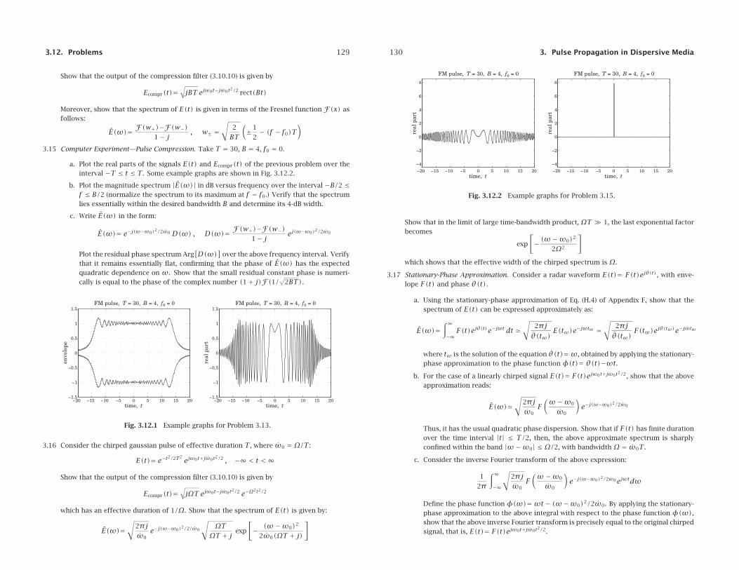
3.12. Problems 129
Show that the output of the compression filter (3.10.10) is given by
Ecompr(t)=√jBT ejω0t−jω0t2/2 rect(Bt)
Moreover, show that the spectrum of E(t) is given in terms of the Fresnel function F(x) asfollows:
E(ω)= F(w+)−F(w−)1− j , w± =
√2
BT
(±1
2− (f − f0)T
)
3.15 Computer Experiment—Pulse Compression. Take T = 30, B = 4, f0 = 0.
a. Plot the real parts of the signals E(t) and Ecompr(t) of the previous problem over theinterval −T ≤ t ≤ T. Some example graphs are shown in Fig. 3.12.2.
b. Plot the magnitude spectrum |E(ω)| in dB versus frequency over the interval −B/2 ≤f ≤ B/2 (normalize the spectrum to its maximum at f = f0.) Verify that the spectrumlies essentially within the desired bandwidth B and determine its 4-dB width.
c. Write E(ω) in the form:
E(ω)= e−j(ω−ω0)2/2ω0 D(ω) , D(ω)= F(w+)−F(w−)1− j ej(ω−ω0)2/2ω0
Plot the residual phase spectrum Arg[D(ω)
]over the above frequency interval. Verify
that it remains essentially flat, confirming that the phase of E(ω) has the expectedquadratic dependence on ω. Show that the small residual constant phase is numeri-cally is equal to the phase of the complex number (1+ j)F(1/√2BT).
−20 −15 −10 −5 0 5 10 15 20−1.5
−1
−0.5
0
0.5
1
1.5
time, t
enve
lope
FM pulse, T = 30, B = 4, f0 = 0
−20 −15 −10 −5 0 5 10 15 20−1.5
−1
−0.5
0
0.5
1
1.5
time, t
real
par
t
FM pulse, T = 30, B = 4, f0 = 0
Fig. 3.12.1 Example graphs for Problem 3.13.
3.16 Consider the chirped gaussian pulse of effective duration T, where ω0 = Ω/T:
E(t)= e−t2/2T2ejω0t+jω0t2/2 , −∞ < t <∞
Show that the output of the compression filter (3.10.10) is given by
Ecompr(t)=√jΩT ejω0t−jω0t2/2 e−Ω
2t2/2
which has an effective duration of 1/Ω. Show that the spectrum of E(t) is given by:
E(ω)=√
2πjω0
e−j(ω−ω0)2/2/ω0
√ΩT
ΩT + j exp
[− (ω−ω0)2
2ω0(ΩT + j)
]
130 3. Pulse Propagation in Dispersive Media
−20 −15 −10 −5 0 5 10 15 20−4
−2
0
2
4
6
8
time, t
real
par
t
FM pulse, T = 30, B = 4, f0 = 0
−20 −15 −10 −5 0 5 10 15 20−4
−2
0
2
4
6
8
time, t
real
par
t
FM pulse, T = 30, B = 4, f0 = 0
Fig. 3.12.2 Example graphs for Problem 3.15.
Show that in the limit of large time-bandwidth product,ΩT� 1, the last exponential factorbecomes
exp
[−(ω−ω0)2
2Ω2
]
which shows that the effective width of the chirped spectrum is Ω.
3.17 Stationary-Phase Approximation. Consider a radar waveform E(t)= F(t)ejθ(t), with enve-lope F(t) and phase θ(t).
a. Using the stationary-phase approximation of Eq. (H.4) of Appendix F, show that thespectrum of E(t) can be expressed approximately as:
E(ω)=∫ ∞−∞F(t)ejθ(t)e−jωt dt �
√2πjθ(tω)
E(tω)e−jωtω =√
2πjθ(tω)
F(tω)ejθ(tω)e−jωtω
where tω is the solution of the equation θ(t)=ω, obtained by applying the stationary-phase approximation to the phase function φ(t)= θ(t)−ωt.
b. For the case of a linearly chirped signal E(t)= F(t)ejω0t+jω0t2/2, show that the aboveapproximation reads:
E(ω)�√
2πjω0
F(ω−ω0
ω0
)e−j(ω−ω0)2/2ω0
Thus, it has the usual quadratic phase dispersion. Show that if F(t) has finite durationover the time interval |t| ≤ T/2, then, the above approximate spectrum is sharplyconfined within the band |ω−ω0| ≤ Ω/2, with bandwidth Ω = ω0T.
c. Consider the inverse Fourier transform of the above expression:
1
2π
∫ ∞−∞
√2πjω0
F(ω−ω0
ω0
)e−j(ω−ω0)2/2ω0ejωtdω
Define the phase function φ(ω)=ωt− (ω−ω0)2/2ω0. By applying the stationary-phase approximation to the above integral with respect to the phase function φ(ω),show that the above inverse Fourier transform is precisely equal to the original chirpedsignal, that is, E(t)= F(t)ejω0t+jω0t2/2.
3.12. Problems 131
d. Apply the compression filter (3.10.10) to the approximate spectrum of Part b, and showthat the corresponding compressed signal is in the time domain:
Ecompr(t)=√jω0
2πejω0t F(−ω0t)
where F(ω) is the Fourier transform of F(t). This is similar, but not quite identical,to the exact expression (3.10.14).
e. Show that Part c is a general result. Consider the stationary-phase approximationspectrum of Part a. Its inverse Fourier transform is:
1
2π
∫ ∞−∞
√2πjθ(tω)
F(tω)ejθ(tω)e−jωtωejωtdω
Define the phase function φ(ω)= θ(tω)−ωtω+ωt. Show that the stationary-phaseapproximation applied to this integral with respect to the phase functionφ(ω) recov-ers the original waveform E(t)= F(t)ejθ(t).[Hint: the condition θ(tω)=ω implies θ(tω)(dtω/dω)= 1.]
3.18 An envelope signal F(t) is processed through two successive pulse compression filters withchirping parameters ω1 and ω2, as shown below.
where Gi(ω)= ejω2/2ωi , i = 1,2. Show that if the chirping parameter of the intermediatequadratic modulation is chosen to be ω0 = ω1+ω2, then the overall output is a time-scaledversion of the input:
Fout(t)= j√ω2
ω1ejω0ω2t2/2ω1 F
(−ω2tω1
)
4Propagation in Birefringent Media
4.1 Linear and Circular Birefringence
In this chapter, we discuss wave propagation in anisotropic media that are linearly or cir-cularly birefringent. In such media, uniform plane waves can be decomposed in two or-thogonal polarization states (linear or circular) that propagate with two different speeds.The two states develop a phase difference as they propagate, which alters the total po-larization of the wave. Such media are used in the construction of devices for generatingdifferent polarizations.
Linearly birefringent materials can be used to change one polarization into another,such as changing linear into circular. Examples are the so-called uniaxial crystals, suchas calcite, quartz, ice, tourmaline, and sapphire.
Optically active or chiral media are circularly birefringent. Examples are sugar solu-tions, proteins, lipids, nucleic acids, amino acids, DNA, vitamins, hormones, and virtuallymost other natural substances. In such media, circularly polarized waves go throughunchanged, with left- and right-circular polarizations propagating at different speeds.This difference causes linearly polarized waves to have their polarization plane rotateas they propagate—an effect known as natural optical rotation.
A similar but not identical effect—the Faraday rotation—takes place in gyroelec-tric media, which are ordinary isotropic materials (glass, water, conductors, plasmas)subjected to constant external magnetic fields that break their isotropy. Gyromagneticmedia, such as ferrites subjected to magnetic fields, also become circularly birefringent.
We discuss all four birefringent cases (linear, chiral, gyroelectric, and gyromagnetic)and the type of constitutive relationships that lead to the corresponding birefringentbehavior. We begin by casting Maxwell’s equations in different polarization bases.
An arbitrary polarization can be expressed uniquely as a linear combination of twopolarizations along two orthogonal directions.† For waves propagating in the z-direction,we may use the two linear directions {x, y}, or the two circular ones for right and leftpolarizations {e+, e−}, where e+ = x − jy and e− = x + jy.‡ Indeed, we have thefollowing identity relating the linear and circular bases:
†For complex-valued vectors e1, e2, orthogonality is defined with conjugation: e∗1 · e2 = 0.‡Note that e± satisfy: e∗± · e± = 2, e∗+ · e− = 0, e+ × e− = 2j z, and z× e± = ±j e±.
![Anisotropic and dispersive wave propagation within strain ... · as di erent quantities. ... 2006]. Indeed, ... In its basic formulation, elastic wave propagation within PAM shares](https://img.pdfslide.us/doc/110x75/5b2af4347f8b9a3e228b4664/anisotropic-and-dispersive-wave-propagation-within-strain-as-di-erent-quantities.jpg)


![Ece Vi Antennas and Propagation [10ec64] Notes](https://img.pdfslide.us/doc/110x75/55cf9bb1550346d033a70934/ece-vi-antennas-and-propagation-10ec64-notes.jpg)