Pulsar analysis with LAT data:A quick tutorial

Massimiliano Razzano(INFN-Pisa)

Fermi Meeting,

(1 Oct. 2009)

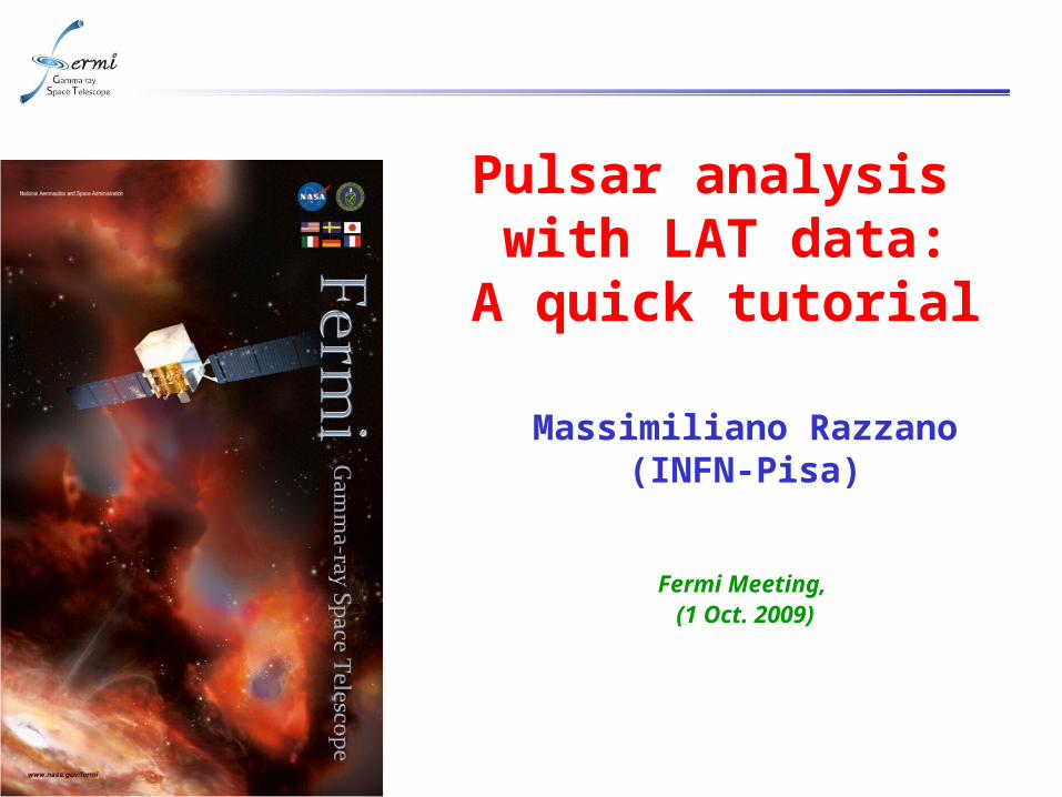
Pulsar Analysis

Timing

Spatial

(point source)

Identification

(periodicity)

Spectrum

(likelihood)

Known pulsar

Gamma-ray selected pulsar

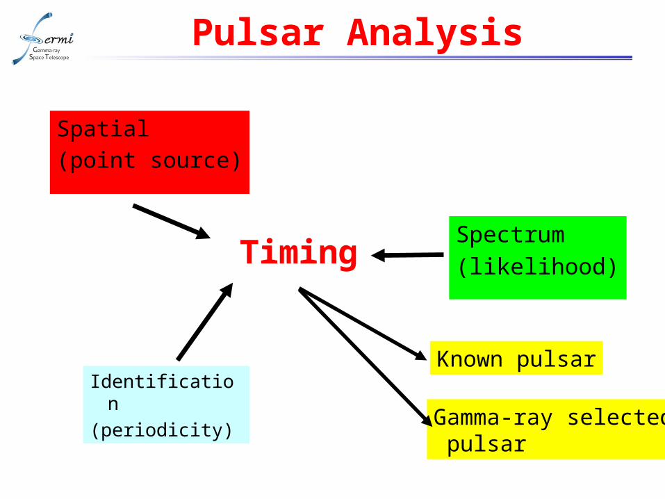
Overview

Overview• In this tutorial we will see how to perform timing analysis of

pulsars using official Fermi tools.• In particular:

– Extracting pulsar spin parameters;– Data selection according to ephemeris validity;– Barycentric corrections;– Rotational phase assignment;– Periodicity test;– Periodicity (basic) search;– Orbital phase assignment;

• A dataset is provided for the exercise• We will not see:

– Blind search– TEMPO2,PRESTO,etc…

• The diffuse Galactic emission is bright and highly structured. The diffuse model supplied by the LAT team has recently been updated and is likely to continue to evolve. Separating weaker sources from the diffuse Galactic emission is non-trivial.

• The LAT Instrument Response Functions (IRFs) have significant uncertainties at energies near 100 MeV and a non-negligible charged particle background at energies above 10 GeV. Improvements in the IRFs are expected but are not imminent.

Where Things Get Complicated

• If you are searching for a source that is not in the LAT catalog, then it is probably weak enough that a simple analysis will not be adequate.

• If you need a detailed energy spectrum or are looking for particular spectral features, especially at very low or very high energies, the LAT team has experience with non-standard analysis.

• If you are trying to analyze the Galactic Center region, you are strongly advised not to go it alone!

• If you are interested in the most complete multiwavelength coverage, consider contacting the LAT team. We have many cooperating groups across the spectrum who may be interested in working with you (even if you don’t include the LAT team).

Some Occasions to Think about Contacting the Instrument Team

Data for the tutorial

• We have prepared a dataset of LAT data using the LAT data server of the FSSC

• The chosen pulsar is PSR J2021+3651 in Cygnus, one of the first new pulsars studied with the LAT, located in the “Dragonfly” PWN.

• Dataset contains:– FT1 file ranging from MJD 54690 (Aug 12 2008) to MJD 54790 (Nov

20 2008); – Corresponding FT2;

• Analysis of pulsars observed in other energies require a database with the ephemeris: we call it D4 database

• The D4 used contains radio observations of J2021+3651 by GBT, as used in the Fermi paper (Abdo et al. ApJ 700, 1059 2009)

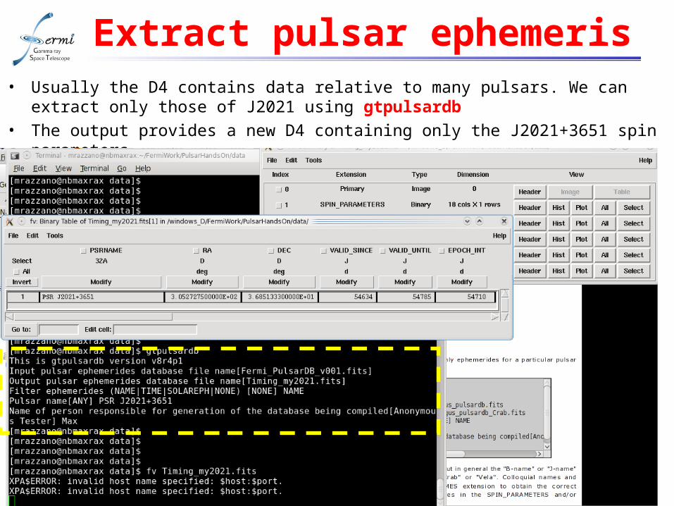
Extract pulsar ephemeris• Usually the D4 contains data relative to many pulsars. We can extract only those of

J2021 using gtpulsardb

• The output provides a new D4 containing only the J2021+3651 spin parameters.

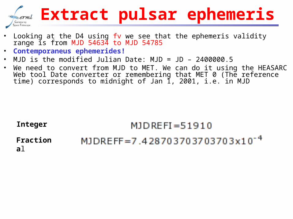
Extract pulsar ephemeris• Looking at the D4 using fv we see that the ephemeris validity range is from MJD

54634 to MJD 54785• Contemporaneus ephemerides!• MJD is the modified Julian Date: MJD = JD – 2400000.5• We need to convert from MJD to MET. We can do it using the HEASARC Web tool

Date converter or remembering that MET 0 (The reference time) corresponds to midnight of Jan 1, 2001, i.e. in MJD

Integer

Fractional

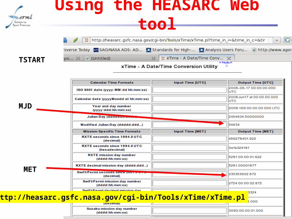
Using the HEASARC Web tool

MJD

MET

TSTART

http://heasarc.gsfc.nasa.gov/cgi-bin/Tools/xTime/xTime.pl

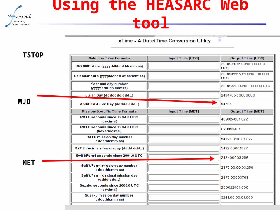
Using the HEASARC Web tool

MJD

MET

TSTOP

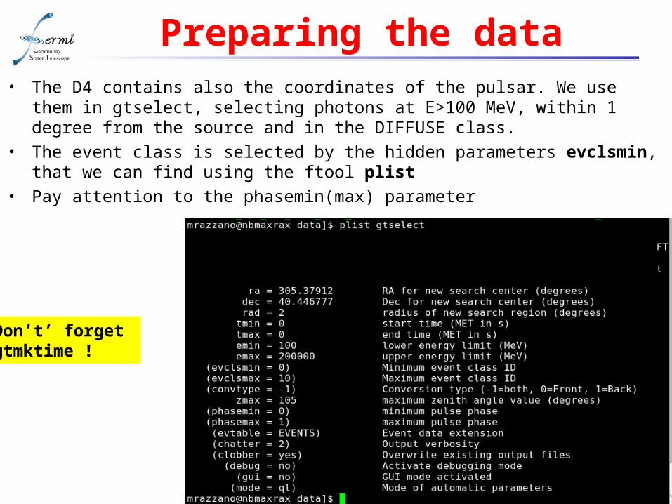
Preparing the data• The D4 contains also the coordinates of the pulsar. We use them in gtselect,

selecting photons at E>100 MeV, within 1 degree from the source and in the DIFFUSE class.

• The event class is selected by the hidden parameters evclsmin, that we can find using the ftool plist

• Pay attention to the phasemin(max) parameter

Don’t’ forget gtmktime !

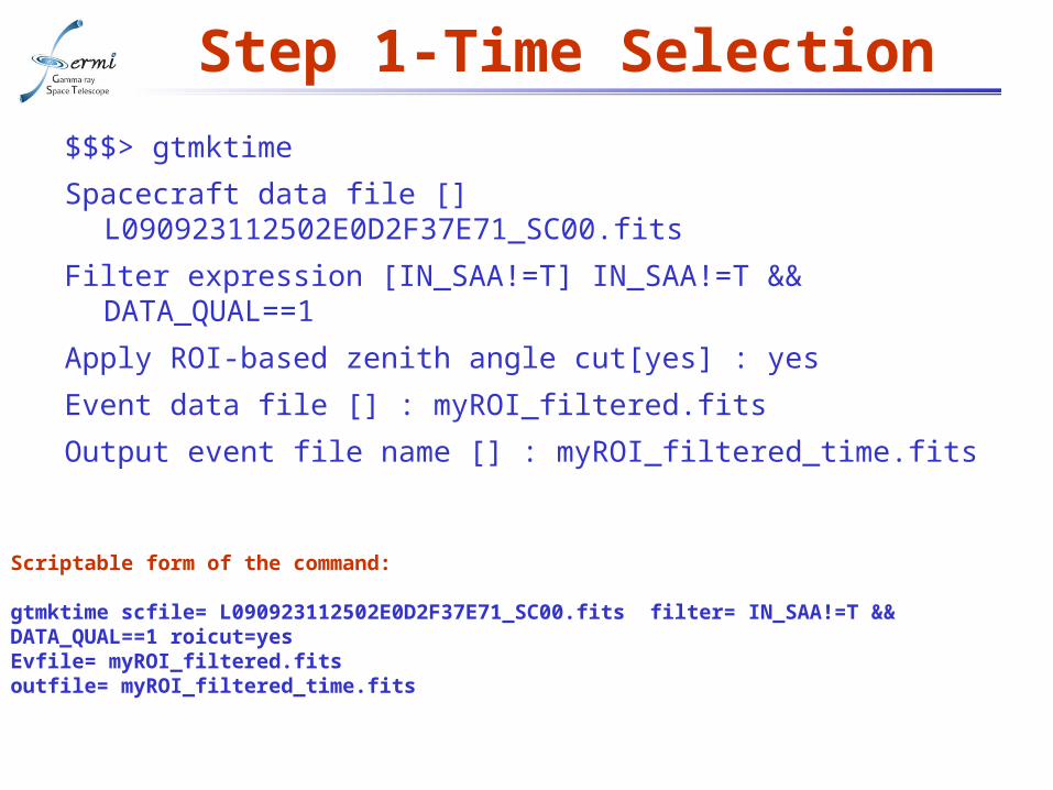
Step 1-Time Selection

$$$> gtmktime

Spacecraft data file [] L090923112502E0D2F37E71_SC00.fits

Filter expression [IN_SAA!=T] IN_SAA!=T && DATA_QUAL==1

Apply ROI-based zenith angle cut[yes] : yes

Event data file [] : myROI_filtered.fits

Output event file name [] : myROI_filtered_time.fits

Scriptable form of the command:

gtmktime scfile= L090923112502E0D2F37E71_SC00.fits filter= IN_SAA!=T && DATA_QUAL==1 roicut=yesEvfile= myROI_filtered.fitsoutfile= myROI_filtered_time.fits

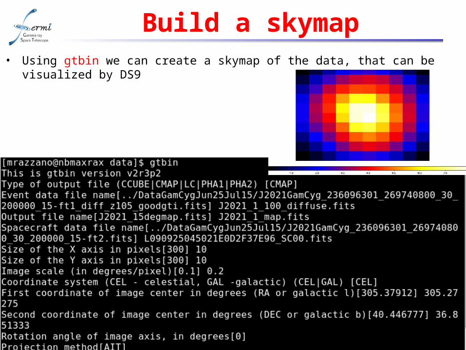
Build a skymap• Using gtbin we can create a skymap of the data, that can be visualized by DS9

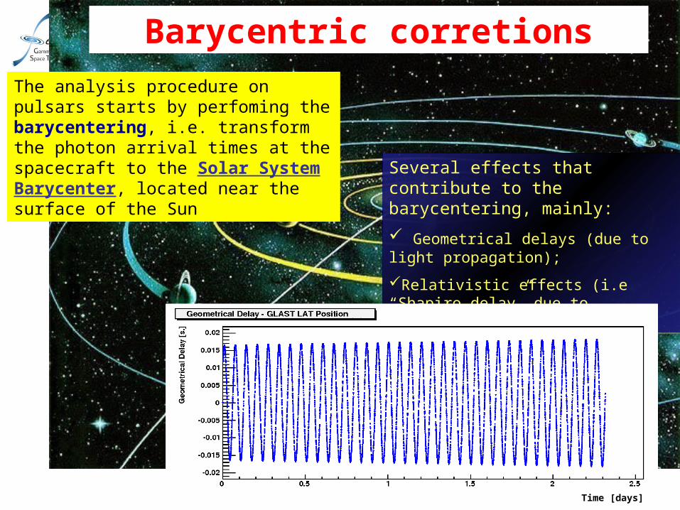
Barycentric corretions

The analysis procedure on pulsars starts by perfoming the barycentering, i.e. transform the photon arrival times at the spacecraft to the Solar System Barycenter, located near the surface of the Sun

Several effects that contribute to the barycentering, mainly:

Geometrical delays (due to light propagation);

Relativistic effects (i.e “Shapiro delay” due to gravitational wall of Sun)

Several effects that contribute to:the barycentering, mainly

Geometrical delays (due to light;(propagation

Relativistic effects (i.e “Shapiro delay” due to gravitational wall of(Sun

Time [days]

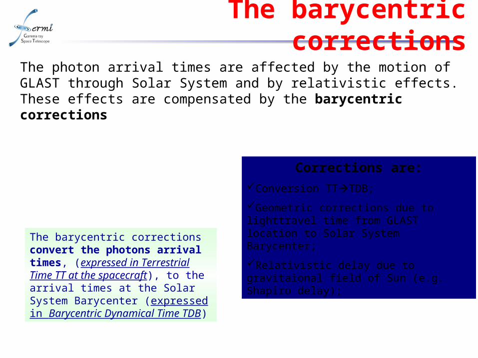
The barycentric corrections

The barycentric corrections convert the photons arrival times, (expressed in Terrestrial Time TT at the spacecraft), to the arrival times at the Solar System Barycenter (expressed in Barycentric Dynamical Time TDB)

The photon arrival times are affected by the motion of GLAST through Solar System and by relativistic effects. These effects are compensated by the barycentric corrections

Corrections are:Conversion TTTDB;

Geometric corrections due to lighttravel time from GLAST location to Solar System Barycenter;

Relativistic delay due to gravitaional field of Sun (e.g. Shapiro delay);

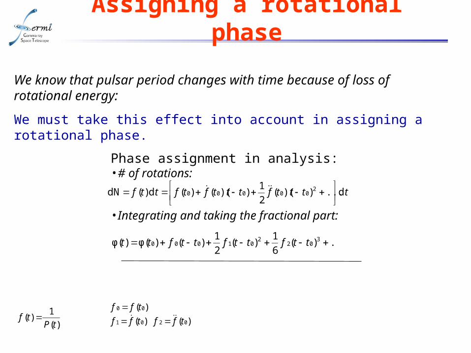
Assigning a rotational phase

Phase assignment in analysis:•# of rotations:

•Integrating and taking the fractional part:

ttttftttftfttf d...))((2

1))(()(d)(dN 2

00000

...)(6

1)(

2

1)()φ()φ( 3

022

01000 ttfttfttftt

)( 00 tff )( 01 tff )( 02 tff )(

1)(

tPtf

We know that pulsar period changes with time because of loss of rotational energy:

We must take this effect into account in assigning a rotational phase.

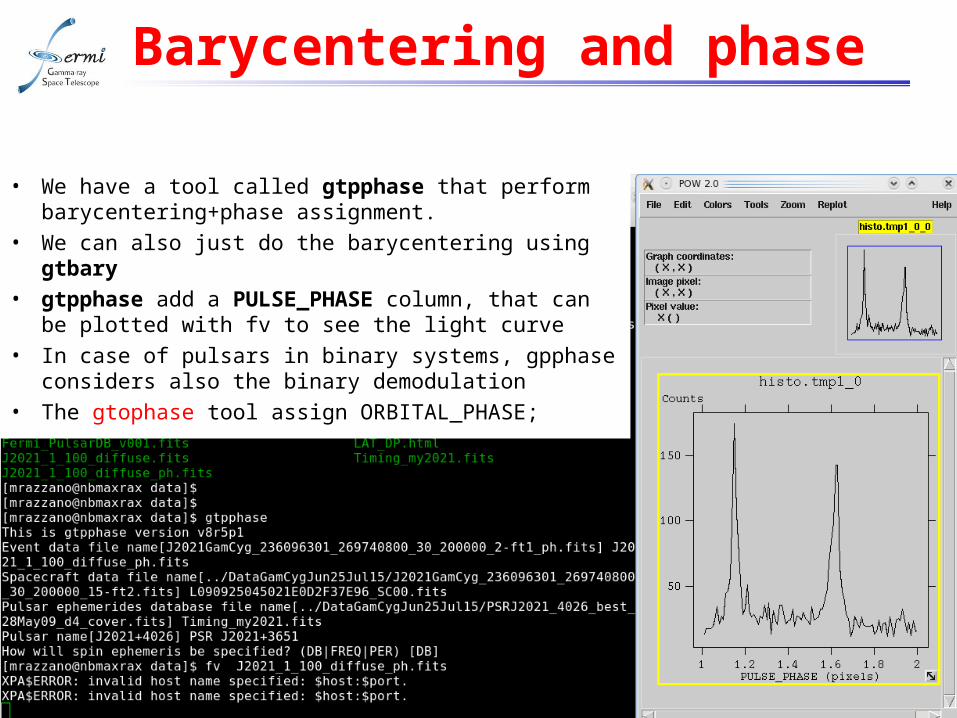
Barycentering and phase

• We have a tool called gtpphase that perform barycentering+phase assignment.

• We can also just do the barycentering using gtbary

• gtpphase add a PULSE_PHASE column, that can be plotted with fv to see the light curve

• In case of pulsars in binary systems, gpphase considers also the binary demodulation

• The gtophase tool assign ORBITAL_PHASE;

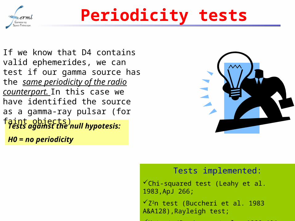
Periodicity tests

Tests implemented:Chi-squared test (Leahy et al. 1983,ApJ 266;

Z2n test (Buccheri et al. 1983 A&A128),Rayleigh test;

H test (De Jager et al., 1989 A&A 221)

Tests against the null hypotesis:

H0 = no periodicity

If we know that D4 contains valid ephemerides, we can test if our gamma source has the same periodicity of the radio counterpart. In this case we have identified the source as a gamma-ray pulsar (for faint objects)

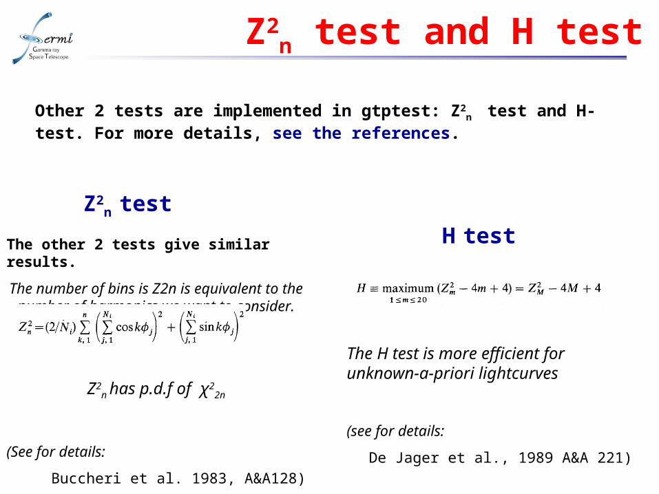
Z2n test and H test

Other 2 tests are implemented in gtptest: Z2n test and H-test. For more

details, see the references.

The other 2 tests give similar results.

The number of bins is Z2n is equivalent to the number of harmonics we want to consider.

Z2n has p.d.f of χ2

2n

(See for details:

Buccheri et al. 1983, A&A128)

Z2n test

The H test is more efficient for unknown-a-priori lightcurves

(see for details:

De Jager et al., 1989 A&A 221)

H test

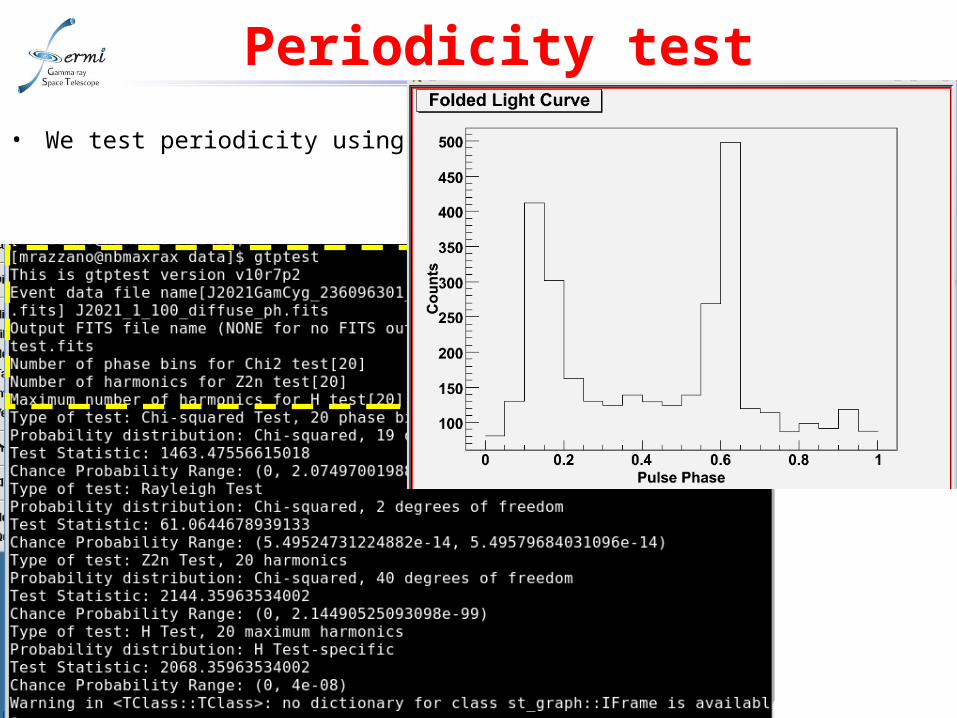
Periodicity test

• We test periodicity using gtptest

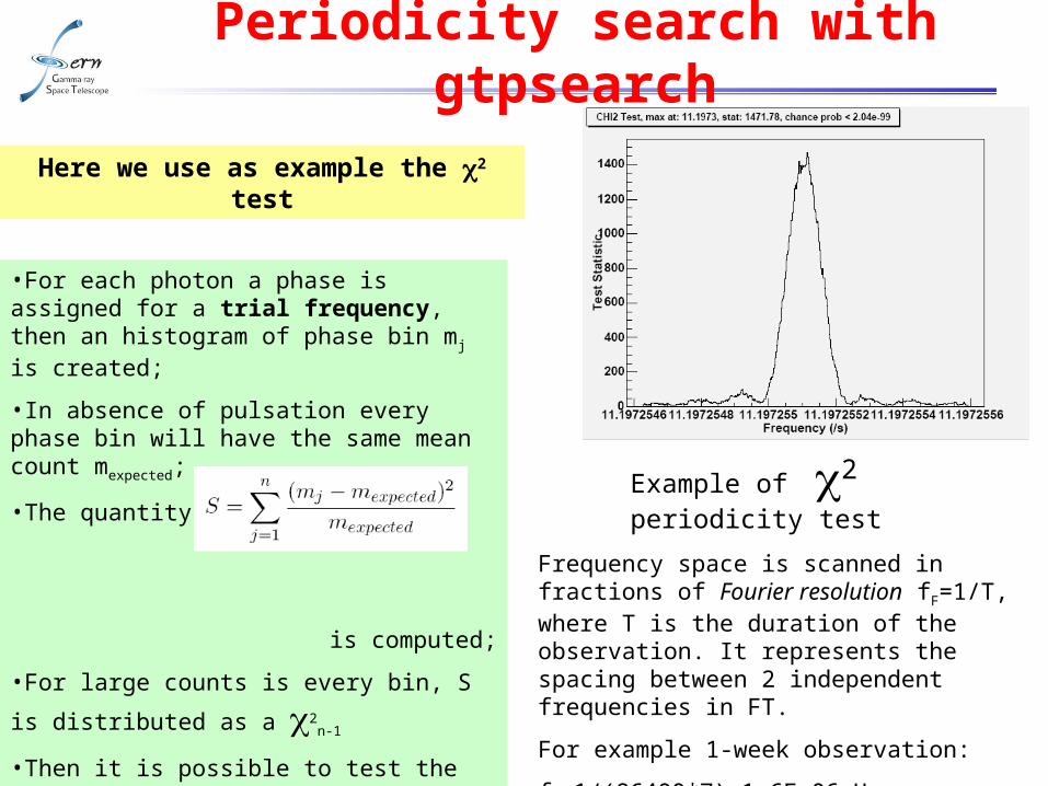
Periodicity search with gtpsearch

Here we use as example the 2 test

•For each photon a phase is assigned for a trial frequency, then an histogram of phase bin mj is created;

•In absence of pulsation every phase bin will have the same mean count mexpected;

•The quantity:

is computed;

•For large counts is every bin, S is distributed

as a 2n-1

•Then it is possible to test the non-periodicity hypothesis and give a chance probability p(2>S)

Example of 2 periodicity test

Frequency space is scanned in fractions of Fourier resolution fF=1/T, where T is the duration of the observation. It represents the spacing between 2 independent frequencies in FT.

For example 1-week observation:

fF 1/(86400*7)≈1.6E-06 Hz

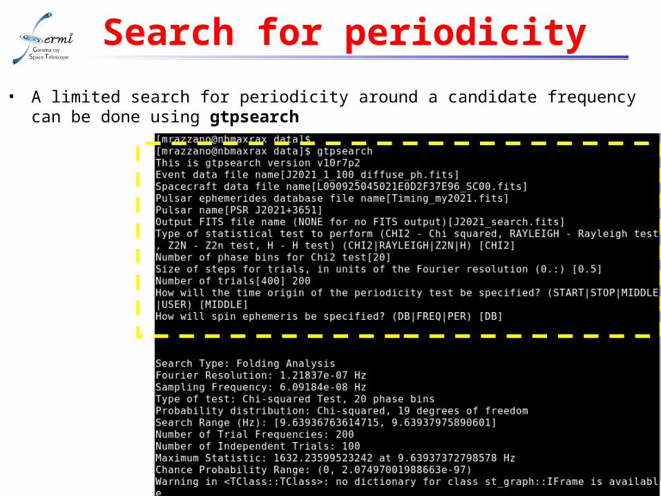
Search for periodicity

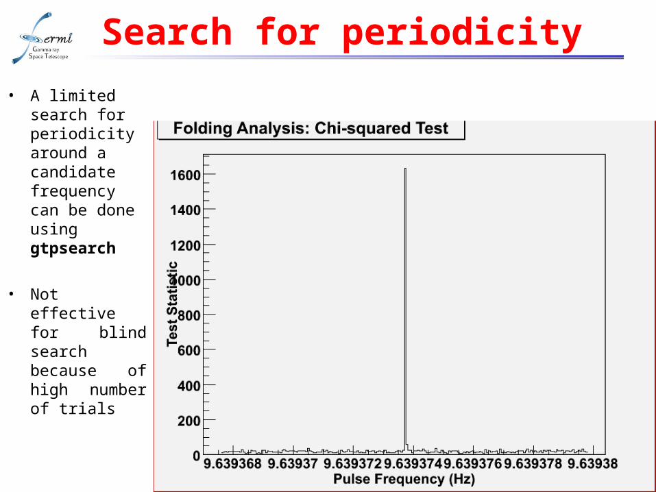
• A limited search for periodicity around a candidate frequency can be done using gtpsearch

Search for periodicity

• A limited search for periodicity around a candidate frequency can be done using gtpsearch

• Not effective for blind search because of high number of trials

Manipulating ephemerides

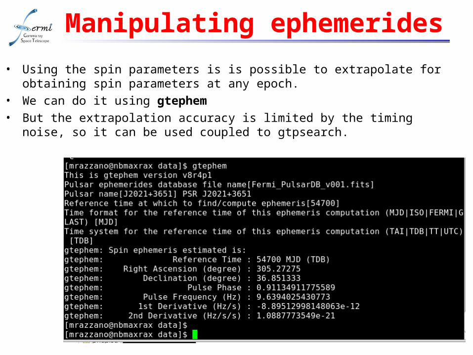
• Using the spin parameters is is possible to extrapolate for obtaining spin parameters at any epoch.

• We can do it using gtephem

• But the extrapolation accuracy is limited by the timing noise, so it can be used coupled to gtpsearch.

ConclusionsConclusions

• Basic pulsar analysis can be performed using official Fermi tools

• Spectral analysis can be done with standard likelihood

• By combining general tools (i.e. gtselect) and pulsar-specific tools (i.e. gtptest), more complex analyses can be done (i.e. light curve evolution with energy)

• The data provided should allow some practice with this analysis

• We chosen a bright pulsar. With faintest ones the data selection is much more important

Enjoy your favourite pulsar !