Embed Size (px)
Citation preview

CHAPTER 30
Publication Bias
IntroductionThe problem of missing studiesMethods for addressing biasIllustrative exampleThe modelGetting a sense of the dataIs there evidence of any bias?Is the entire effect an artifact of bias?How much of an impact might the bias have?Summary of the findings for the illustrative exampleSome important caveatsSmall-study effectsConcluding remarks
INTRODUCTION
While a meta-analysis will yield a mathematically accurate synthesis of the studies
included in the analysis, if these studies are a biased sample of all relevant studies, then
the mean effect computed by the meta-analysis will reflect this bias. Several lines of
evidence show that studies that report relatively high effect sizes are more likely to be
published than studies that report lower effect sizes. Since published studies are more
likely to find their way into a meta-analysis, any bias in the literature is likely to be
reflected in the meta-analysis as well. This issue is generally known as publication bias.
The problem of publication bias is not unique to systematic reviews. It affects the
researcher who writes a narrative review and even the clinician who is searching a
database for primary papers. Nevertheless, it has received more attention with
regard to systematic reviews and meta-analyses, possibly because these are pro-
moted as being more accurate than other approaches to synthesizing research.
In this chapter we first discuss the reasons for publication bias and the evidence
that it exists. Then we discuss a series of methods that have been developed to assess
Introduction to Meta-Analysis. Michael Borenstein, L. V. Hedges, J. P. T. Higgins and H. R. Rothstein © 2009 John Wiley & Sons, Ltd. ISBN: 978-0-470-05724-7

the likely impact of bias in any given meta-analysis. At the end of the chapter we
present an illustrative example.
THE PROBLEM OF MISSING STUDIES
When planning a systematic review we develop a set of inclusion criteria that
govern the types of studies that we want to include. Ideally, we would be able to
locate all studies that meet our criteria, but in the real world this is rarely possible.
Even with the advent of (and perhaps partly due to an over-reliance on) electronic
searching, it is likely that some studies which meet our criteria will escape our
search and not be included in the analysis.
If the missing studies are a random subset of all relevant studies, the failure to
include these studies will result in less information, wider confidence intervals, and
less powerful tests, but will have no systematic impact on the effect size. However,
if the missing studies are systematically different than the ones we were able to
locate, then our sample will be biased. The specific concern is that studies that
report relatively large effects for a given question are more likely to be published
than studies that report smaller effects for the same question. This leads to a bias in
the published literature, which then carries over to a meta-analysis that draws on this
literature.
Studies with significant results are more likely to be published
Several lines of research (reviewed by Dickersin, 2005) have established that studies
with statistically significant results are more likely to find their way into the published
literature than studies that report results that are not statistically significant. And, for any
given sample size the result is more likely to be statistically significant if the effect size
is larger. It follows that if there is a population of studies that looked at the magnitude of
a relationship, and the observed effects are distributed over a range of values (as they
always are), the studies with effects toward the higher end of that range are more likely
to be statistically significant and therefore to be published. This tendency has the
potential to produce very large biases in the magnitude of the relationships, particularly
if studies have relatively small sample sizes (see, Hedges, 1984; 1989).
A particularly enlightening line of research was to identify groups of studies
as they were initiated, and then follow them prospectively over a period of
years to see which were published and which were not. This approach was
taken by Easterbrook, Berlin, Gopalan, & Matthews (1991), Dickersin, Min, &
Meinert (1992), Dickersin & Min (1993a), among others. Nonsignificant
studies were less likely to be published than significant studies (61–86% as
likely), and when published were subject to longer delay prior to publication.
Similar studies have demonstrated that researchers selectively report their
findings in the reports they do publish, sometimes even changing what is
labeled a priori as the main hypothesis (Chan et al., 2004).
278 Other Issues

Published studies are more likely to be included in a meta-analysis
If persons performing a systematic review were able to locate studies that had been
published in the grey literature (any literature produced in electronic or print format
that is not controlled by commercial publishers, such as technical reports and
similar sources), then the fact that the studies with higher effects are more likely
to be published in the more mainstream publications would not be a problem for
meta-analysis. In fact, though, this is not usually the case.
While a systematic review should include a thorough search for all relevant
studies, the actual amount of grey/unpublished literature included, and the types,
varies considerably across meta-analyses. When Rothstein (2006) reviewed the 95
meta-analytic reviews published in Psychological Bulletin between 1995 and 2005 to
see whether they included unpublished or grey research, she found that 23 of the 95
clearly did not include any unpublished data. Clarke and Clarke (2000) studied the
references from healthcare protocols and reviews published in The Cochrane Library
in 1999, and found that about 92% of references to studies included in reviews were
to journal articles. Of the remaining 8%, about 4% were to conference proceedings,
about 2% were to unpublished material (for example personal communication, in
press documents and data on file), and slightly over 1% were to books or book
chapters. In a similar vein, Mallet, Hopewell, & Clarke (2002) looked at the sources
of grey literature included in the first 1000 Cochrane systematic reviews, and found
that nearly half of them did not include any data from grey or unpublished sources.
Since the meta-analyses published in the Cochrane Database have been shown to
retrieve a higher proportion of studies than those published in many journals, these
estimates probably understate the extent of the problem.
Some have suggested that it is legitimate to exclude studies that have not been
published in peer-reviewed journals because these studies tend to be of lower quality.
For example, in their systematic review, Weisz et al. (1995) wrote ‘We included only
published psychotherapy outcome studies, relying on the journal review process as
one step of quality control’ (p. 452). However, it is not obvious that journal review
assures high quality, nor that it is the only mechanism that can do so. For one thing,
not all researchers aim to publish their research in academic journals. For example,
researchers working for government agencies, independent think-tanks or consulting
firms generally focus on producing reports, not journal articles. Similarly, a thesis or
dissertation may be of high quality, but is unlikely to be submitted for publication in
an academic journal if the individual who produced it is not pursuing an academic
career. And of course, peer review may be biased, unreliable, or of uneven quality.
Overall, then, publication status cannot be used as a proxy for quality; and in our
opinion should not be used as a basis for inclusion or exclusion of studies.
Other sources of bias
Other factors that can lead to an upward bias in effect size and are included under the
umbrella of publication bias are the following. Language bias (English-language
Chapter 30: Publication Bias

databases and journals are more likely to be searched, which leads to an over-
sampling of statistically significant studies) (Egger et al., 1997; Juni et al., 2002);
availability bias (selective inclusion of studies that are easily accessible to the
researcher); cost bias (selective inclusion of studies that are available free or at low
cost); familiarity bias (selective inclusion of studies only from one’s own discipline);
duplication bias (studies with statistically significant results are more likely to be
published more than once (Tramer et al., 1997)) and citation bias (whereby studies
with statistically significant results are more likely to be cited by others and therefore
easier to identify (Gøtzsche, 1997; Ravnskov, 1992)).
METHODS FOR ADDRESSING BIAS
In sum, it is possible that the studies in a meta-analysis may overestimate the true
effect size because they are based on a biased sample of the target population of
studies. But how do we deal with this concern? The only true test for publication
bias is to compare effects in the published studies formally with effects in the
unpublished studies. This requires access to the unpublished studies, and if we had
that we would no longer be concerned. Nevertheless, the best approach would be for
the reviewer to perform a truly comprehensive search of the literature, in hopes of
minimizing the bias. In fact, there is evidence that this approach is somewhat
effective. Cochrane reviews tend to include more studies and to report a smaller
effect size than similar reviews published in medical journals. Serious efforts to find
unpublished, and difficult to find studies, typical of Cochrane reviews, may there-
fore reduce some of the effects of publication bias.
Despite the increased resources that are needed to locate and retrieve data from
sources such as dissertations, theses, conference papers, government and techni-
cal reports and the like, it is generally indefensible to conduct a synthesis that
categorically excludes these types of research reports. Potential benefits and costs
of grey literature searches must be balanced against each other. Readers who
would like more guidance in the process of literature searching and information
retrieval may wish to consult Hopewell, Mallett and Clarke (2005), Reed and
Baxter (2009), Rothstein and Hopewell (2009), or Wade, Turner, Rothstein and
Lavenberg (2006).
Since we cannot be certain that we have avoided bias, researchers have developed
methods intended to assess its potential impact on any given meta-analysis. These
methods address the following questions:
� Is there evidence of any bias?
� Is it possible that the entire effect is an artifact of bias?
� How much of an impact might the bias have?
We shall illustrate these methods as they apply to a meta-analysis on passive
smoking and lung cancer.
280 Other Issues

ILLUSTRATIVE EXAMPLE
Hackshaw et al. (1997) published a meta-analysis with data from 37 studies that
reported on the relationship between so-called second-hand (passive) smoking and
lung cancer. The paper reported that exposure to second-hand smoke increased the
risk of lung cancer in the nonsmoking spouse by about 20%. Questions were raised
about the possibility that studies with larger effects were more likely to have been
published (and included in the analysis) than those with smaller (or nil) effects, and
that the conclusion was therefore suspect.
THE MODEL
In order to gauge the impact of publication bias we need a model that tells us which
studies are likely to be missing. The model that is generally used (and the one we
follow here) makes the following assumptions: (a) Large studies are likely to be
published regardless of statistical significance because these involve large commit-
ments of time and resources. (b) Moderately sized studies are at risk for being lost,
but with a moderate sample size even modest effects will be significant, and so only
some studies are lost here. (c) Small studies are at greatest risk for being lost.
Because of the small sample size, only the largest effects are likely to be significant,
with the small and moderate effects likely to be unpublished.
The combined result of these three items is that we expect the bias to increase as
the sample size goes down, and the methods described below are all based on this
model. Other, more sophisticated methods have been developed for estimating the
number of missing studies and/or adjusting the observed effect to account for bias.
These have rarely been used in actual research because they are difficult to imple-
ment and also because they require the user to make some relatively sophisticated
assumptions and choices.
Before proceeding with the example we call the reader’s attention to an important
caveat. The procedures that we describe here look for a relationship between sample
size and effect size, and if such a relationship is found, it is attributed to the
existence of missing studies. While this is one possible reason that the effect size
is larger in the smaller studies, it is also possible that the effect size really is larger in
the smaller studies. We mention this caveat here to provide a context for the
discussion that follows, and return to it near the end of the chapter, in the section
entitled small-study effects.
GETTING A SENSE OF THE DATA
A good place to start in assessing the potential for bias is to get a sense of the data,
and the forest plot can be used for this purpose. Figure 30.1 is a forest plot of the
studies in the passive smoking meta-analysis. In this example, an increase in risk is
indicated by a risk ratio greater than 1.0. The overwhelming majority of studies
show an increased risk for second-hand smoke, and the last row in the spreadsheet
Chapter 30: Publication Bias
shows the summary data for the fixed-effect model. The risk ratio is 1.204 and the
95% confidence interval is 1.120 to 1.295.
The studies have been plotted from most precise to least precise, so that larger
studies appear toward the top and smaller studies appear toward the bottom. This
has no impact on the summary effect, but it allows us to see the relationship between
sample size and effect size. As we move toward the bottom of the plot the effects
shift toward the right, which is what the model would predict if bias is present.
If the analysis includes some studies from peer-reviewed journals and others from
the grey literature, we can also group by source and see if the grey papers (which may
be representative of any missing studies) tend to have smaller effects than the others.
The funnel plot
Another mechanism for displaying the relationship between study size and effect
size is the funnel plot.
Figure 30.1 Passive smoking and lung cancer – forest plot.
282 Other Issues

Traditionally, the funnel plot wasplotted with effect size on the X axisand the sample
size or variance on the Y axis. Large studies appear toward the top of the graph and
generally cluster around the meaneffect size. Smaller studies appear toward the bottom
of the graph, and (since smaller studies have more sampling error variation in effect
sizes) tend to be spread across a broad range of values. This pattern resembles a funnel,
hence the plot’s name (Light and Pillemer, 1984; Light et al., 1994).
The use of the standard error (rather than sample size or variance) on the Y axis
has the advantage of spreading out the points on the bottom half of the scale, where
the smaller studies are plotted. This could make it easier to identify asymmetry.
This affects the display only, and has no impact on the statistics, and this is the route
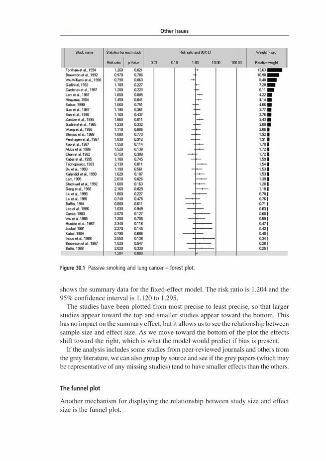
we follow here (Figure 30.2).
IS THERE EVIDENCE OF ANY BIAS?
In the absence of publication bias, the studies will be distributed symmetrically
about the mean effect size, since the sampling error is random. In the presence of
publication bias the studies are expected to follow the model, with symmetry at the
top, a few studies missing in the middle, and more studies missing near the bottom.
If the direction of the effect is toward the right (as in our example), then near the
bottom of the plot we expect a gap on the left, where the nonsignificant studies
would have been if we had been able to locate them.
In the running example (Figure 30.2) the risk ratio (in log units) is at the bottom
and the standard error is on the Y axis (which has been reversed, so low values are at
–2.0 –1.5 –1.0 –0.5 0.0 0.5 1.0 1.5 2.0
0.0
0.2
0.4
0.6
0.8
Sta
ndar
d E
rror
Log risk ratio
Funnel Plot of Standard Error by Log risk ratio
Figure 30.2 Passive smoking and lung cancer – funnel plot.
Chapter 30: Publication Bias

the top). The subjective impression does support the presence of asymmetry.
Toward the bottom of the graph most studies appear toward the right (indicating
more risk), which is consistent with the possibility that some studies are missing
from the left.
First, we ask if there is evidence of any bias. Because the interpretation of a funnel
plot is largely subjective, several tests have been proposed to quantify or test the
relationship between sample size and effect size. Two early proposals are in
common use (Begg and Mazumdar, 1994, Egger et al., 1997); a comprehensive
review appears in Chapter 10 of Higgins and Green (2008).
While these tests provide useful information, several caveats are in order.
First, the tests (like the funnel plot) may yield a very different picture
depending on the index used in the analysis (risk difference versus risk
ratio, for example). Second, this approach makes sense only if there is a
reasonable amount of dispersion in the sample sizes and a reasonable number
of studies. Third, even when these criteria are met, the tests tend to have
lower power. Therefore, the absence of a significant correlation or regression
cannot be taken as evidence of symmetry.
In any event, even if we could somehow solve these problems, the question
addressed by the tests (is there evidence of any bias) is of limited import. A more
interesting question would be How much bias is there, and what is its impact on our
conclusions?
IS THE ENTIRE EFFECT AN ARTIFACT OF BIAS?
The next question one might ask is whether or not the observed overall effect is
robust. In other words, can we be confident that the effect is not solely an artifact of
bias?
Rosenthal’s Fail-safe N
An early approach to dealing with publication bias was Rosenthal’s Fail-safe N.
Suppose a meta-analysis reports a significant p-value based on k studies. We are
concerned that studies with smaller effects are missing, and if we were to retrieve all
the missing studies and include them in the analysis, the p-value for the summary
effect would no longer be significant. Rosenthal (1979) suggested that we actually
compute how many missing studies we would need to retrieve and incorporate in the
analysis before the p-value became nonsignificant. For purposes of this exercise we
would assume that the mean effect in the missing studies was zero. If it should
emerge that we needed only a few studies (say, five or ten) to ‘nullify’ the effect,
then we would be concerned that the true effect was indeed zero. However, if it
turned out that we needed a large number of studies (say, 20,000) to nullify the
effect, there would be less reason for concern.
284 Other Issues

Rosenthal referred to this as a File drawer analysis (file drawers being the
presumed location of the missing studies), and Harris Cooper suggested that the
number of missing studies needed to nullify the effect should be called the
Fail-safe N (Rosenthal, 1979; Begg and Mazumdar, 1994).
While Rosenthal’s work was critical in focusing attention on publication
bias, this approach is of limited utility for a number of reasons. First, it focuses
on the question of statistical significance rather than substantive significance.
That is, it asks how many hidden studies are required to make the effect not
statistically significant, rather than how many hidden studies are required
to reduce the effect to the point that it is not of substantive importance.
Second, the formula assumes that the mean effect size in the hidden studies is
zero, when in fact it could be negative (which would require fewer studies to
nullify the effect) or positive but low. Finally, the Fail-safe N is based on
significance tests that combine p-values across studies, as was common at the
time that Rosenthal suggested the method. Today, the common practice is to
compute a summary effect, and then compute the p-value for this effect. The
p-values computed using the different approaches actually test different null
hypotheses, and are not the same. For these reasons this approach is not generally
appropriate for analyses that focus on effect sizes. We have addressed it at
relative length only because the method is well known and because of its
important historical role.
That said, for the passive smoking review the Fail-safe N is 398, suggesting
that there would need to be nearly 400 studies with a mean risk ratio of 1.0 added to
the analysis, before the cumulative effect would become statistically nonsignificant.
Orwin’s Fail-safe N
As noted, two problems with Rosenthal’s approach are that it focuses on statistical
significance rather than substantive significance, and that it assumes that the mean
effect size in the missing studies is zero. Orwin (1983) proposed a variant on the
Rosenthal formula that addresses both of these issues. First, Orwin’s method allows
the researcher to determine how many missing studies would bring the overall effect
to a specified level other than zero. The researcher could therefore select a value that
would represent the smallest effect deemed to be of substantive importance, and ask
how many missing studies it would take to bring the summary effect below this
point. Second, it allows the researcher to specify the mean effect in the missing
studies as some value other than zero. This would allow the researcher to model a
series of other distributions for the missing studies (Becker, 2005; Begg and
Mazumdar, 1994).
In the running example, Orwin’s Fail-safe N is 103, suggesting that there would
need to be over 100 studies with a mean risk ratio of 1.0 added to the analysis before
the cumulative effect would become trivial (defined as a risk ratio of 1.05).
Chapter 30: Publication Bias
HOW MUCH OF AN IMPACT MIGHT THE BIAS HAVE?
The approaches outlined above ask whether bias has had any impact on the observed
effect (those based on the funnel plot), or whether it might be entirely responsible
for the observed effect (Fail-safe N). As compared with these extreme positions, a
third approach attempts to estimate how much impact the bias had, and to estimate
what the effect size would have been in the absence of bias. The hope is to classify
each meta-analysis into one of three broad groups, as follows.
� The impact of bias is probably trivial. If all relevant studies were included the
effect size would probably remain largely unchanged.
� The impact of bias is probably modest. If all relevant studies were included the
effect size might shift but the key finding (that the effect is, or is not, of
substantive importance) would probably remain unchanged.
� The impact of bias may be substantial. If all relevant studies were included, the
key finding (that the effect size is, or is not, of substantive importance) could
change.
Duval and Tweedie’s Trim and Fill
As discussed above, the key idea behind the funnel plot is that publication bias may
be expected to lead to asymmetry. If there are more small studies on the right than
on the left, our concern is that there may be studies missing from the left. (In the
running example we expect suppression of studies on the left, but in other cases we
would expect suppression on the right. The algorithm requires the reviewer to
specify the expected direction.)
Trim and Fill uses an iterative procedure to remove the most extreme small studies
from the positive side of the funnel plot, re-computing the effect size at each iteration
until the funnel plot is symmetric about the (new) effect size. In theory, this will yield
an unbiased estimate of the effect size. While this trimming yields the adjusted effect
size, it also reduces the variance of the effects, yielding a too narrow confidence
interval. Therefore, the algorithm then adds the original studies back into the analysis,
and imputes a mirror image for each. This fill has no impact on the point estimate but
serves to correct the variance (Duval and Tweedie, 2000a, 2000b).
A major advantage of this approach is that it addresses an important question,
What is our best estimate of the unbiased effect size? Another nice feature of this
approach is that it lends itself to an intuitive visual display. The computer programs
that incorporate Trim and Fill are able to create a funnel plot that includes both the
observed studies and the imputed studies, so the researcher can see how the effect
size shifts when the imputed studies are included. If this shift is trivial, then one can
have more confidence that the reported effect is valid. A problem with this method
is that it depends strongly on the assumptions of the model for why studies are
missing, and the algorithm for detecting asymmetry can be influenced by one or two
aberrant studies.
286 Other Issues

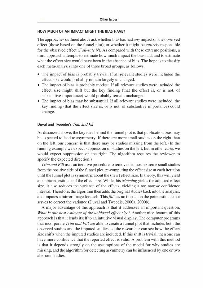
We can re-display the funnel plot, taking into account the Trim and Fill adjust-
ment. In Figure 30.3, the observed studies are shown as open circles, and the
observed point estimate in log units is shown as an open diamond at 0.185 (0.113,
0.258), corresponding to a risk ratio of 1.204 (1.120, 1.295). The seven imputed
studies are shown as filled circles, and the imputed point estimate in log units is
shown as a filled diamond at 0.156 (0.085, 0.227), corresponding to a risk ratio of
1.169 (1.089, 1.254). The ‘adjusted’ point estimate suggests a lower risk than the
original analysis. Perhaps the key point, though, is that the adjusted estimate is fairly
close to the original – in this context, a risk ratio of 1.17 has the same substantive
implications as a risk ratio of 1.20.
Restricting analysis to the larger studies
If publication bias operates primarily on smaller studies, then restricting the analy-
sis to large studies, which might be expected to be published irrespective of their
results, would in theory overcome any problems. The question then arises as to what
threshold defines a large study. We are unable to offer general guidance on this
question. A potentially useful strategy is to illustrate all possible thresholds by
drawing a cumulative meta-analysis.
A cumulative meta-analysis is a meta-analysis run first with one study, then
repeated with a second study added, then a third, and so on. Similarly, in a
cumulative forest plot, the first row shows the effect based on one study, the second
–2.0 –1.5 –1.0 –0.5 0.0 0.5 1.0 1.5 2.0
0.0
0.2
0.4
0.6
0.8
Sta
ndar
d E
rror
Log risk ratio
Funnel Plot of Standard Error by Log risk ratio
Figure 30.3 Passive smoking and lung cancer – funnel plot with imputed studies.
Chapter 30: Publication Bias

row shows the cumulative effect based on two studies, and so on. We discuss
cumulative meta-analysis in more detail in Chapter 42.
To examine the effect of different thresholds for study size, the studies are sorted
in the sequence of largest to smallest (or of most precise to least precise), and a
cumulative meta-analysis performed with the addition of each study. If the point
estimate has stabilized with the inclusion of the larger studies and does not shift with
the addition of smaller studies, then there is no reason to assume that the inclusion of
smaller studies had injected a bias (i.e. since it is the smaller studies in which study
selection is likely to be greatest). On the other hand, if the point estimate does shift
when the smaller studies are added, then there is at least a prima facie case for bias,
and one would want to investigate the reason for the shift.
This approach also provides an estimate of the effect size based solely on the larger
studies. And, even more so than Trim and Fill, this approach is entirely transparent:
We compute the effect based on the larger studies and then determine if and how the
Figure 30.4 Passive smoking and lung cancer – cumulative forest plot.
288 Other Issues

effect shifts with the addition of the smaller studies (a clear distinction between larger
and smaller studies will not usually exist, but is not needed).
Figure 30.4 shows a cumulative forest plot of the data. Note the difference between
thecumulativeplotandthestandardversionshownearlier.Here, thefirst rowisa‘meta’
analysis based only on the Fontham et al. study. The second row is a meta-analysis
basedontwostudies (Fonthametal. andBrownsonetal.),andsoon.Thelast study tobe
added is Butler (1988), and so the point estimate and confidence interval shown on the
line labeled ‘Butler’ are identical to that shown for the summary effect on the line
labeled ‘Fixed’. Note that the scale on this plot is 0.50 to 2.00.
The studies have been sorted from the most precise to the least precise (roughly
corresponding to largest tosmallest). With the 18 largest studies in the analysis, starting
at the top (inclusive of Chan and Fung, 1982) the cumulative relative risk is 1.15. With
the addition of another 19 (smaller) studies, the point estimate shifts to the right, and the
relative risk is 1.20. As such, our estimate of the relative risk has increased. However,
the key point is that even if we had limited the analysis to the 18 larger studies, the
relative risk would have been 1.15 (with 95% confidence interval of 1.07, 1.25) and the
clinical implications probably would have been the same.
Note also that the analysis that incorporates all 37 studies assigns 83% of its
weight to the first 18 (see the bar graph in the right-hand column). In other words, if
small studies are introducing a bias, we are protected to some extent by the fact that
small studies are given less weight. Recall, however, that random-effects meta-
analyses award relatively more weight to smaller studies than fixed-effect meta-
analyses, so a cumulative meta-analysis based on a random-effects model may not
reveal such protection.
A major advantage of this approach is that it provides an estimate of the unbiased
effect size (under the strong assumptions of the model) and lends itself to an
intuitive visual display. Unlike Trim and Fill, this approach will not be thrown by
one or two aberrant studies.
SUMMARY OF THE FINDINGS FOR THE ILLUSTRATIVE EXAMPLE
The various statistical procedures approach the problem of bias from a number of
directions. One would not expect the results of the different procedures to ‘match’
each other since the procedures ask different questions. Rather, the goal should
be to synthesize the different pieces of information provided by the various
procedures.
Getting a sense of the data
There are a substantial number of studies in this analysis. While the vast majority
show an increased risk, only a few are statistically significant. This suggests that the
mechanism of publication bias based on statistical significance was not a powerful
one in this case.
Chapter 30: Publication Bias

Is there evidence of bias?
The funnel plot is noticeably asymmetric, with a majority of the smaller studies
clustering to the right of the mean. This visual impression is confirmed by Egger’s
test which yields a statistically significant p-value. The rank correlation test did not
yield a significant p-value, but this could be due to the low power of the test. As a
whole the smaller studies did tend to report a higher association between passive
smoking and lung cancer than did the larger studies.
Is it possible that the observed relationship is entirely an artifact of bias?
Rosenthal’s Fail-safe N is 398, suggesting that there would need to be nearly 400 studies
with a mean risk ratio of 1.0 added to the analysis, before the cumulative effect would
become statistically nonsignificant. Similarly, Orwin’s Fail-safe N is 103, suggesting
that there would need to be over 100 studies with a mean risk ratio of 1.0 added to the
analysis before the cumulative effect would become trivial (defined as a risk ratio of
1.05). Given that the authors of the meta-analysis were able to identify only 37 studies
that looked at the relationship of passive smoking and lung cancer, it is unlikely that
nearly 400 studies, or even 103 studies, were missed. While we may have overstated the
risk caused by second-hand smoke, it is unlikely that the actual risk is zero.
What impact might the bias have on the risk ratio?
The complete meta-analysis showed that passive smoking was associated with a 20%
increase in risk of lung cancer. By contrast, the meta-analysis based on the larger studies
reported an increased risk of 16%. Similarly, the Trim and Fill method suggested that
if we removed the asymmetric studies, the increased risk would be imputed as 15%.
Earlier, we suggested that the goal of a publication bias analysis should be to
classify the results into one of three categories (a) where the impact of bias is trivial,
(b) where the impact is not trivial but the major finding is still valid, and (c) where
the major finding might be called into question. This meta-analysis seems to fall
squarely within category b. There is evidence of larger effects in the smaller studies,
which is consistent with our model for publication bias. However, there is no reason
to doubt the validity of the core finding, that passive smoking is associated with a
clinically important increase in the risk of lung cancer.
SOME IMPORTANT CAVEATS
Most of the approaches discussed in this chapter look for evidence that the effect
sizes are larger in the smaller studies, and interpret this as reflecting publication
bias. This relationship between effect size and sample size lies at the core of the
forest plot, as well as the correlation and regression tests. It also drives the algorithm
for Trim and Fill and the logic of restricting the analysis to the larger studies.
Therefore, it is important to be aware that these procedures are subject to a
number of caveats. They may yield a very different picture depending on the
290 Other Issues

index used in the analysis (e.g. risk difference versus risk ratio). The procedures can
easily miss real dispersion. They have the potential to work only if there is a
reasonable amount of dispersion in the sample sizes and also a reasonable number
of studies. Even when these conditions are met, the tests (correlation and regression)
tend to have lower power. Therefore, our failure to find evidence of asymmetry
should not lead to a false sense of assurance.
SMALL-STUDY EFFECTS
Equally important, when there is clear evidence of asymmetry, we cannot assume
that this reflects publication bias. The effect size may be larger in small studies
because we retrieved a biased sample of the smaller studies, but it is also possible
that the effect size really is larger in smaller studies for entirely unrelated reasons.
For example, the small studies may have been performed using patients who were
quite ill, and therefore more likely to benefit from the drug (as is sometimes the case
in early trials of a new compound). Or, the small studies may have been performed
with better (or worse) quality control than the larger ones. Sterne et al. (2001) use
the term small-study effect to describe a pattern where the effect is larger in small
studies, and to highlight the fact that the mechanism for this effect is not known.
Adjustments for publication bias should always be made with this caveat in mind.
For example, we should report ‘If the asymmetry is due to bias, our analyses suggest
that the adjusted effect would fall in the range of . . .’ rather than asserting ‘the
asymmetry is due to bias, and therefore the true effect falls in the range of . . .’
CONCLUDING REMARKS
It is almost always important to include an assessment of publication bias in relation
to a meta-analysis. It will either assure the reviewer that the results are robust, or
alert them that the results are suspect. This is important to ensure the integrity of the
individual meta-analysis. It is also important to ensure the integrity of the field.
When a meta-analysis ignores the potential for bias and is later found to be
incorrect, the perception is fostered that meta-analyses cannot be trusted.
SUMMARY POINTS
� Publication bias exists when the studies included in the analysis differ system-
atically from all studies that should have been included. Typically, studies
with larger than average effects are more likely to be published, and this can
lead to an upward bias in the summary effect.
� Methods have been developed to assess the likely impact of publication bias on
any given meta-analysis. Using these methods we report that if we adjusted the
Chapter 30: Publication Bias

CONTINUED
effect to remove the bias, (a) the resulting effect would be essentially
unchanged, or (b) the effect might change but the basic conclusion, that the
treatment works (or not) would not be changed, or (c) the basic conclusion
would be called into question.
� Methods developed to address publication bias require us to make many
assumptions, including the assumption that the pattern of results is due to
bias, and that this bias follows a certain model.
� Publication bias is a problem for meta-analysis, but also a problem for
narrative reviews or for persons performing any search of the literature.
Further reading
Chalmers, T.C., Frank, C.S., & Reitman, D. (1990). Minimizing the three states of publication
bias. JAMA 263: 1392–1395.
Dickersin, K., Chan, S., Cha.mers,T.C., Sacks, H.S., & Smith, H. (1987) Publication bias in
clinical trials. Controlled Clinical Trials 8: 348–353.
Dickersin, K,. Min, Y.L., & Meinert, C.L. (1992). Factors influencing publication of research results:
Follow-up of applications submitted to two institutional review boards. JAMA 267: 374–378.
Hedges, L.V. (1984) Estimation of effect size under nonrandom sampling: The effects of
censoring studies yielding statistically insignificant mean differences. Journal of
Educational Statistics, 9, 61–85.
Hedges, L.V. (1989) Estimating the normal mean and variance under a selection model. In Gleser,
L, Perlman, M.D., Press, S.J., Sampson, A.R. Contributions to Probability and Statistics:
Essays in Honor of Ingram Olkin (pp. 447–458). NY: Springer Verlag.
Hunt, M.M. (1999) The New Know-Nothings: The Political Foes of the Scientific Study of Human
Nature. New Brunswick, NJ, Transacation.
International Committee of Medical Journal Editors. Uniform Requirements for Manuscripts
Submitted to Biomedical Journals: Writing and Editing for Biomedical Publication. Updated
October 2007. Available at http://www.icmje.org/#clin_trials.
Ioannidis, J.P. (2007). Why most published research findings are false: author’s reply to Goodman
and Greenland. PLoS Med 4: e215.
Lau, J., Ioannidis, J.P., Terrin, N., Schmid, C.H., & Olkin, I. (2006). The case of the misleading
funnel plot. BMJ 333: 597–600.
Rosenthal, R. (1979). The ‘File drawer problem’ and tolerance for null results. Psychol Bull 86:
638–641.
Rothstein, H.R., Sutton, A.J., & Borenstein, M. (2005). Publication Bias in Meta-analysis:
Prevention, Assessment and Adjustments. Chichester, UK, John Wiley & Sons, Ltd.
Sterne, J.A., Egger, M. & Smith, G. D. (2001). Systematic reviews in healthcare: investigating
and dealing with publication and other biases in meta-analysis. Bmj 323: 101–105.
Sterne, J.A., Egger, M. (2001). Funnel plots for detecting bias in meta-analysis: guidelines on
choice of axis. J Clin Epidemiol 54: 1046–1055.
Sutton A.J., Duval S.J., Tweedie, R.L., Abrams, K.R., & Jones, D.R. (2000). Empirical
assessment of effect of publication bias on meta-analyses. BMJ 320: 1574–1577.
292 Other Issues