Public Transportation's Contribution to US Greenhouse Gas Reduction

THIS PAGE IS INTENTIONALLY LEFT BLANK

Public Transportation’s Contribution to U.S. Greenhouse Gas Reduction

September 2007

Submitted by: Science Applications International Corporation (SAIC)

Authors: Todd Davis Monica Hale

SAIC

Energy Solutions Operation 8301 Greensboro Drive, MS E-4-6

McLean, VA 22102

SCIENCE APPLICATIONS INTERNATIONAL CORPORATION

iv


PUBLIC TRANSPORTATION’S CONTRIBUTION TO U.S. GREENHOUSE GAS REDUCTION

v

Acknowledgements This study was conducted for the American Public Transportation Association (APTA) with funding provided through the Transit Cooperative Research Program (TCRP) Project J-11/Task 2. The TCRP is sponsored by the Federal Transit Administration (FTA); directed by the Transit Development Corporation, the education and research arm of the APTA; and administered by the National Academies, through the Transportation Board. The report was prepared by SAIC.

Disclaimer The opinions and conclusions expressed or implied are those of the research agency that performed the research and are not necessarily those of the Federal Transit Administration, Transportation Research Board (TRB) or its sponsors. This report has not been reviewed or accepted by the TRB Executive Committee or the Governing Board of the National Research Council.


vi



vii

Table of Contents Page

Abbreviations ........................................................................................................ xi Executive Summary .............................................................................................. 1 Background and Introduction.............................................................................. 5

U.S. Mobile Greenhouse Gas Emissions, 1990–2004 ...................................... 5 Trends in Travel ................................................................................................ 7 Factors Influencing Growth in Greenhouse Gas Emissions.............................. 10 Potential Role of Public Transportation in Reducing CO2 Emissions ................ 12 Potential Role of Public Transportation in Carbon Exchange Programs........... 15

Bibliography .......................................................................................................... 17 Appendix A ............................................................................................................ 19

Background to Climate Change ........................................................................ 19 The GHG Issue ................................................................................................. 19 Trading Carbon on the Chicago Climate Exchange .......................................... 20 Issues Related to Transit’s Participation in Carbon Trading ............................. 22

Appendix B ............................................................................................................ 25 Outline of Calculation of Transit Carbon Dioxide Savings in 2005.................... 25 References ........................................................................................................ 27

Appendix C ............................................................................................................ 29 Average Household Carbon Footprint in the U.S. ............................................. 29

Appendix D ............................................................................................................ 31 Measures and Metrics ....................................................................................... 31


viii



ix

List of Tables Page

Table 1. U.S. Greenhouse Gas Emissions from All Mobile Sources (Tg CO2 Eq.) .................................................................................... 5

Table 2. U.S. Greenhouse Gas Emissions from Mobile Sources, by Vehicle Type (Tg CO2 Eq.) .............................................................. 6

Table 3. VMT, Public Transit Ridership, Delays and Congestion Costs in U.S....... 9 Table 4. Net U.S. Transit Industry Savings in Metric Tonnes.................................. 13 Table 5. Mass Transit’s Contribution to Reduced VMT per Transit

Passenger Mile ................................................................................ 13 Table 6. Added Ridership for NYC Subway Yields Lower Unit Energy Intensity .... 15

List of Figures Page

Figure 1. Total Daily VMT Trends for Urbanized Areas in U.S. in Millions, 1982-2005 in Thousands................................................................. 7

Figure 2. Total Average Delay Hours for Commuting in U.S. Urbanized Areas...... 8 Figure 3. U.S. Public Transportation Passenger Miles (Millions),

1982-2005 ....................................................................................... 9 Figure 4. The Relationship of U.S. GDP, VMT and other Travel Indicators from

1980 to 2001 (in Percent) ................................................................ 10 Figure 5. Real Price of Gasoline in the U.S., 1970-2006 ........................................ 11 Figure 6. Reduction Schedule for Phase II Members ............................................. 21


x



xi

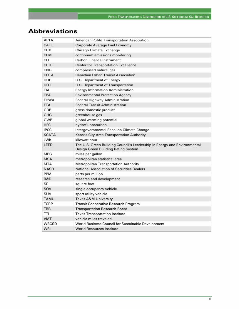
Abbreviations

APTA American Public Transportation Association

CAFE Corporate Average Fuel Economy

CCX Chicago Climate Exchange

CEM continuum emissions monitoring

CFI Carbon Finance Instrument

CFTE Center for Transportation Excellence

CNG compressed natural gas

CUTA Canadian Urban Transit Association

DOE U.S. Department of Energy

DOT U.S. Department of Transportation

EIA Energy Information Administration

EPA Environmental Protection Agency

FHWA Federal Highway Administration

FTA Federal Transit Administration

GDP gross domestic product

GHG greenhouse gas

GWP global warming potential

HFC hydrofluorocarbon

IPCC Intergovernmental Panel on Climate Change

KCATA Kansas City Area Transportation Authority

kWh kilowatt hour

LEED The U.S. Green Building Council’s Leadership in Energy and Environmental

Design Green Building Rating System

MPG miles per gallon

MSA metropolitan statistical area

MTA Metropolitan Transportation Authority

NASD National Association of Securities Dealers

PPM parts per million

R&D research and development

SF square foot

SOV single occupancy vehicle

SUV sport utility vehicle

TAMU Texas A&M University

TCRP Transit Cooperative Research Program

TRB Transportation Research Board

TTI Texas Transportation Institute

VMT vehicle miles traveled

WBCSD World Business Council for Sustainable Development

WRI World Resources Institute


xii



1

Executive Summary

“The scientific debate on the causes of global climate change is basically over – the focus has turned to action”

– Jonathan Lash, Director of the World Resources Institute This report addresses four questions.

1. How much net CO2 is public transportation saving in the U.S .from the current level of

services being offered?

2. How much additional CO2 savings are possible if incremental public transportation

passenger loads are increased?

3. What is the significance of non-public transportation commuter use at a household level

and what can households do to save additional CO2?

4. Are there favorable land use impacts that public transportation contributes to that result

in positive environmental and social benefits?

Answers to these questions show that public transportation is a highly valuable asset for reducing global warming.

1. How much net CO2 is public transportation saving in the U.S. from the current level of services being offered? Answer: Public Transportation is a net CO2 reducer; saving 6.9 million metric tonnes in 2005.

In 2005, public transportation reduced CO2 emissions by 6.9 million metric tonnes. If current public transportation riders were to use personal vehicles instead of transit they would generate 16.2 million metric tonnes of CO2. Actual operation of public transit vehicles, however, resulted in only 12.3 million metric tonnes of these emissions. In addition, 340 million gallons of gasoline were saved through transit’s contribution to decreased congestion, which reduced CO2 emissions by another 3.0 million metric tonnes. An additional 400,000 metric tonnes of greenhouse gases (GHG) were also avoided, including sulfur hexafluoride, hydrofluorocarbons (HFC), perfluorocarbons, and chlorofluorocarbons (CFC).

This study estimated the following benefits of public transportation in 2005 in reducing congestion and this nation’s transportation CO2 emissions:

Metric Tonnes

1. Carbon dioxide emissions from personal vehicles if no transit

service

16.2 million

2. Carbon dioxide emissions from public transportation -12.3 million

3. Net carbon dioxide saved from public transportation 3.9 million

4. Additional carbon dioxide saved from transit reduced

congestion

+3.0 million

5. Total carbon dioxide savings from public transportation 6.9 million

The above referenced 6.9 million metric tonnes of CO2 exceeds the transportation CO2 emissions that exist in the sparsely populated states like North Dakota (6.3 million metric


2

tonnes) and a more densely populated state like Delaware (5.0 million metric tonnes),1 (Environmental Protection Agency [EPA] 2007).

2. How much additional CO2 savings are possible if incremental public transportation passenger ridership is increased? Answer: A solo commuter switching his or her commute to existing public transportation in a single day can reduce their CO2 emissions by 20 pounds or more than 4,800 pounds in a year.

An average private vehicle emission rate is about 1.0 pound of CO2 per mile. An automobile driven by a single person 20 miles round trip to work will emit 20 pounds of CO2. Thus, the savings by using existing service would be about 20.0 pounds of CO2 per daily trip. As passenger loads increase on public transportation, there may be only a slight increase in CO2, much less than driving to work in single occupancy vehicles (SOV). Over the course of a year, an individual could potentially reduce their CO2 emissions by more than 4,800 pounds (assuming 240 days of transit travel per year). This represents slightly more than two metric tonnes of CO2 or about ten percent of a two-car family household’s carbon footprint of 22 metric tonnes per year. In contrast, if one were to weatherize their home and adjust their thermostat the carbon savings would be approximately 2,800 pounds of CO2. Other comparisons include replacing five incandescent bulbs to lower wattage compact fluorescent lamps (445 pounds of CO2 per year), or replacing an older refrigerator freezer (335 pounds of CO2 per year.

3. What is the significance of using more public transportation at a household level and what can households do to save additional CO2? Answer: Public transportation is also effective in reducing household CO2 emissions and cost.

One of the most significant actions that household members can take to reduce their carbon footprint is to use public transportation where it is available. The annual use of an automobile driving an average of 12,000 miles per year and with an average 22.9 miles per gallon (MPG) consumption emits 4.6 metric tonnes of CO2 per year (one metric ton is equivalent to 2,205 pounds). Households that have a sport utility vehicle (SUV) or light duty truck drive and drive an average of 14,500 miles per year with an average MPG of 16.2 emit 7.9 metric tonnes per year.

The carbon footprint of a typical U.S. household is about 22 metric tonnes per year. Reducing the daily use of one low occupancy vehicle and using public transit can reduce a household’s carbon footprint between 25-30%.

4. Are there favorable land use impacts that public transportation contributes to that result in positive environmental and social benefits? Answer: Public transportation provides many benefits that go beyond energy and CO2 savings – as transit assets are being used to accomplish these important functions.

1 http://www.epa.gov/climatechange/emissions/downloads/CO2FFC_2003.pdf


3

Investments in public transportation have the benefit of supporting higher density land uses that allow for fewer vehicle miles of travel. While it is difficult to precisely measure this impact, a number of studies have attempted to estimate the relationship between transit passenger miles and vehicle miles traveled (VMT) reduction as a proxy for this effect. The results range from a reduction in VMT of between 1.4 miles and 9 miles for every transit passenger mile traveled. The outcome would be more efficient use of roadways, reduced road maintenance, shorter highway commute times and reduced need for street and off- street parking.


4



5

Background and Introduction

This report is organized into the following sections:

1. An overview of sources and trends in U.S. mobile GHG emissions; 2. Trends in VMT, congestion levels, annual hours of delay, and cost of delay are

presented for major urbanized areas. This includes a review of trends in passenger miles traveled on public transportation;

3. The primary causal factors stimulating travel and GHGs are reviewed including the rise in U.S. gross domestic product (GDP) and the relatively low real prices of gasoline;

4. Public transportation’s contribution to reducing CO2 emissions; and 5. An overview of the potential role of public transportation in future carbon exchange

programs.

There is a need to reduce CO2 emissions in transportation, but selected key indicators show trends in the other direction.

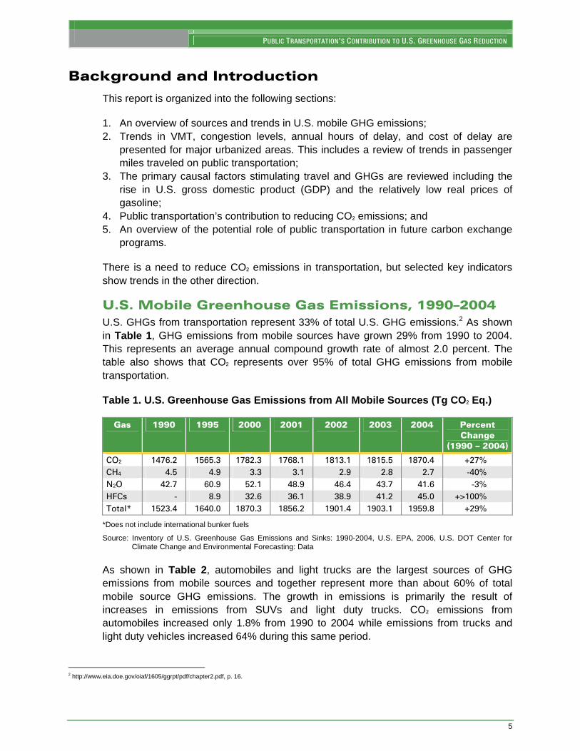
U.S. Mobile Greenhouse Gas Emissions, 1990–2004 U.S. GHGs from transportation represent 33% of total U.S. GHG emissions.2 As shown in Table 1, GHG emissions from mobile sources have grown 29% from 1990 to 2004. This represents an average annual compound growth rate of almost 2.0 percent. The table also shows that CO2 represents over 95% of total GHG emissions from mobile transportation.

Table 1. U.S. Greenhouse Gas Emissions from All Mobile Sources (Tg CO2 Eq.)

Gas 1990 1995 2000 2001 2002 2003 2004 Percent Change

(1990 – 2004)

CO2 1476.2 1565.3 1782.3 1768.1 1813.1 1815.5 1870.4 +27%

CH4 4.5 4.9 3.3 3.1 2.9 2.8 2.7 -40%

N2O 42.7 60.9 52.1 48.9 46.4 43.7 41.6 -3%

HFCs - 8.9 32.6 36.1 38.9 41.2 45.0 +>100%

Total* 1523.4 1640.0 1870.3 1856.2 1901.4 1903.1 1959.8 +29%

*Does not include international bunker fuels

Source: Inventory of U.S. Greenhouse Gas Emissions and Sinks: 1990-2004, U.S. EPA, 2006, U.S. DOT Center for Climate Change and Environmental Forecasting: Data

As shown in Table 2, automobiles and light trucks are the largest sources of GHG emissions from mobile sources and together represent more than about 60% of total mobile source GHG emissions. The growth in emissions is primarily the result of increases in emissions from SUVs and light duty trucks. CO2 emissions from automobiles increased only 1.8% from 1990 to 2004 while emissions from trucks and light duty vehicles increased 64% during this same period.

2 http://www.eia.doe.gov/oiaf/1605/ggrpt/pdf/chapter2.pdf, p. 16.


6

Other GHGs of CH4 and N2O emissions also result from fuel combustion. HFC emissions are associated with motor vehicle air conditioners.

The CO2 emissions reported are based on the carbon content of the different fuels used for different transportation vehicles such as gasoline, diesel fuel, aviation fuel, and residual fuel oil. Subsequent calculations are performed to estimate the share of emissions attributable to different vehicle types and uses.3

Table 2. U.S. Greenhouse Gas Emissions from Mobile Sources, by Vehicle Type (Tg CO2 Eq.)

Vehicles 1990 1995 2000 2001 2002 2003 2004

Cars 646.9 618.3 660.1 661.9 675.9 654.4 658.7

Light Trucks 331.3 413.2 482.5 484.5 495.5 528.6 543.6

Other Highway 234.5 242.6 350.1 348.4 362.0 359.1 377.1

Aircraft 179.1 173.2 195.3 185.4 176.7 173.6 181.5

Marine 44.1 51.7 55.6 48.6 57.6 50.2 54.9

Locomotives 38.2 31.4 45.0 45.2 45.6 47.5 50.3

Mobile Air

Conditioners and

Refrigerated

Transport

- 8.9 32.6 36.1 38.9 41.2 45.0

Other 49.3 100.7 49.1 46.1 49.2 48.5 48.7

Total* 1523.4 1640.0 1870.3 1856.2 1901.4 1903.1 1959.8

Source: Inventory of U.S. Greenhouse Gas Emissions and Sinks: 1990-2004, U.S. Environmental Protection Agency, 2006, U.S. Department of Transportation Center for Climate Change and Environmental Forecasting: Data

U.S. CAFE standards alone do not adequately deal with the rising emissions from the rising levels of VMT. If the growth rate of VMT continues at historical growth rates, the transportation share of GHG emissions will not decline. Recent reports indicate that the time when the planet might be near irreversible global warming has been moved back from stabilization targets of 2025 to within the next ten years.

For a more detailed review of climate change events and risks, see Appendix A.

3 CO2 emissions data are reported in the commonly used “million metric tons” units given its widespread use and more convenient comparisons of various fuel

consumption data having different molecular weights. See a discussion of the use of metric tonnes vs. the molecular weight of various GHG emissions at: http://www.eia.doe.gov/oiaf/1605/gg99rpt/emission_box.html.


7

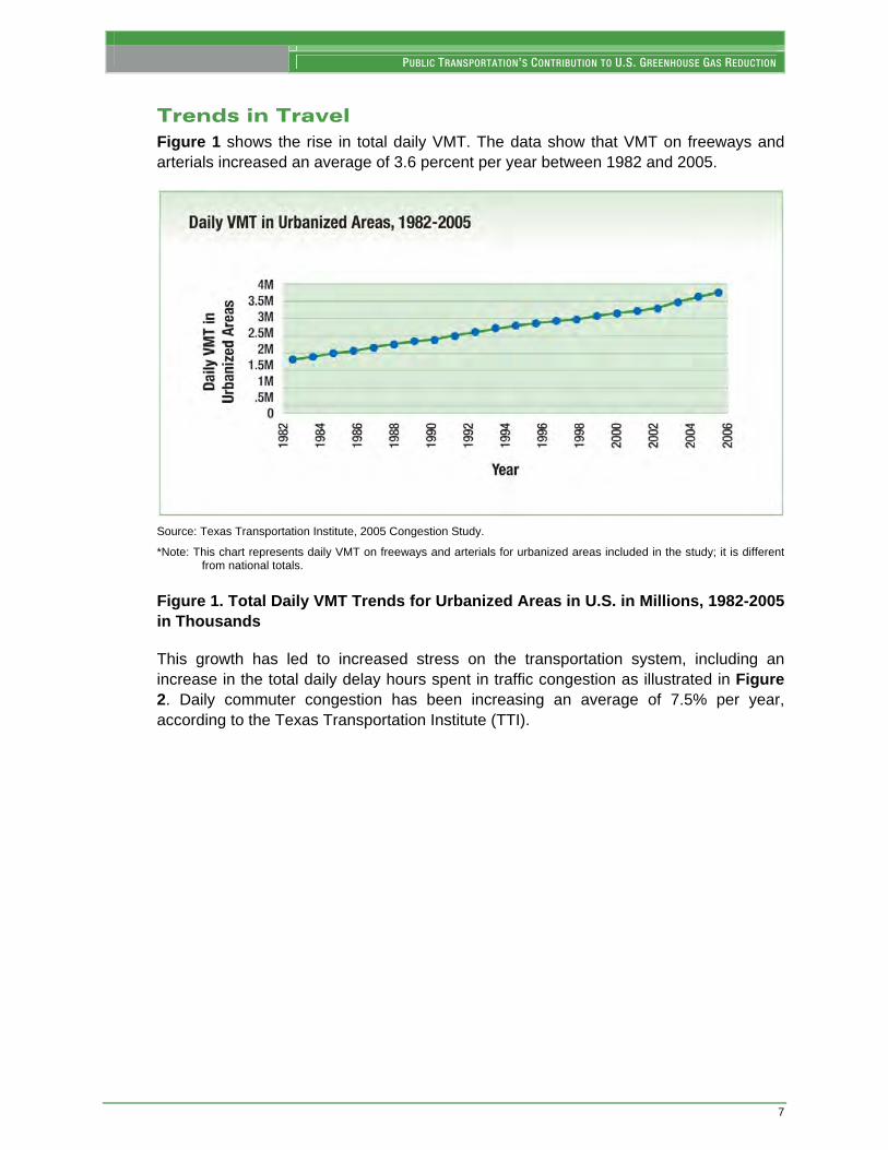
Trends in Travel Figure 1 shows the rise in total daily VMT. The data show that VMT on freeways and arterials increased an average of 3.6 percent per year between 1982 and 2005.

Source: Texas Transportation Institute, 2005 Congestion Study.

*Note: This chart represents daily VMT on freeways and arterials for urbanized areas included in the study; it is different from national totals.

Figure 1. Total Daily VMT Trends for Urbanized Areas in U.S. in Millions, 1982-2005 in Thousands

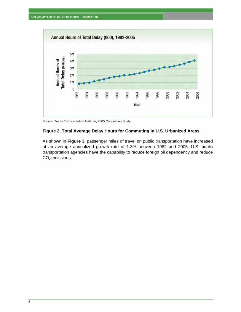
This growth has led to increased stress on the transportation system, including an increase in the total daily delay hours spent in traffic congestion as illustrated in Figure 2. Daily commuter congestion has been increasing an average of 7.5% per year, according to the Texas Transportation Institute (TTI).


8

Source: Texas Transportation Institute, 2005 Congestion Study.

Figure 2. Total Average Delay Hours for Commuting in U.S. Urbanized Areas

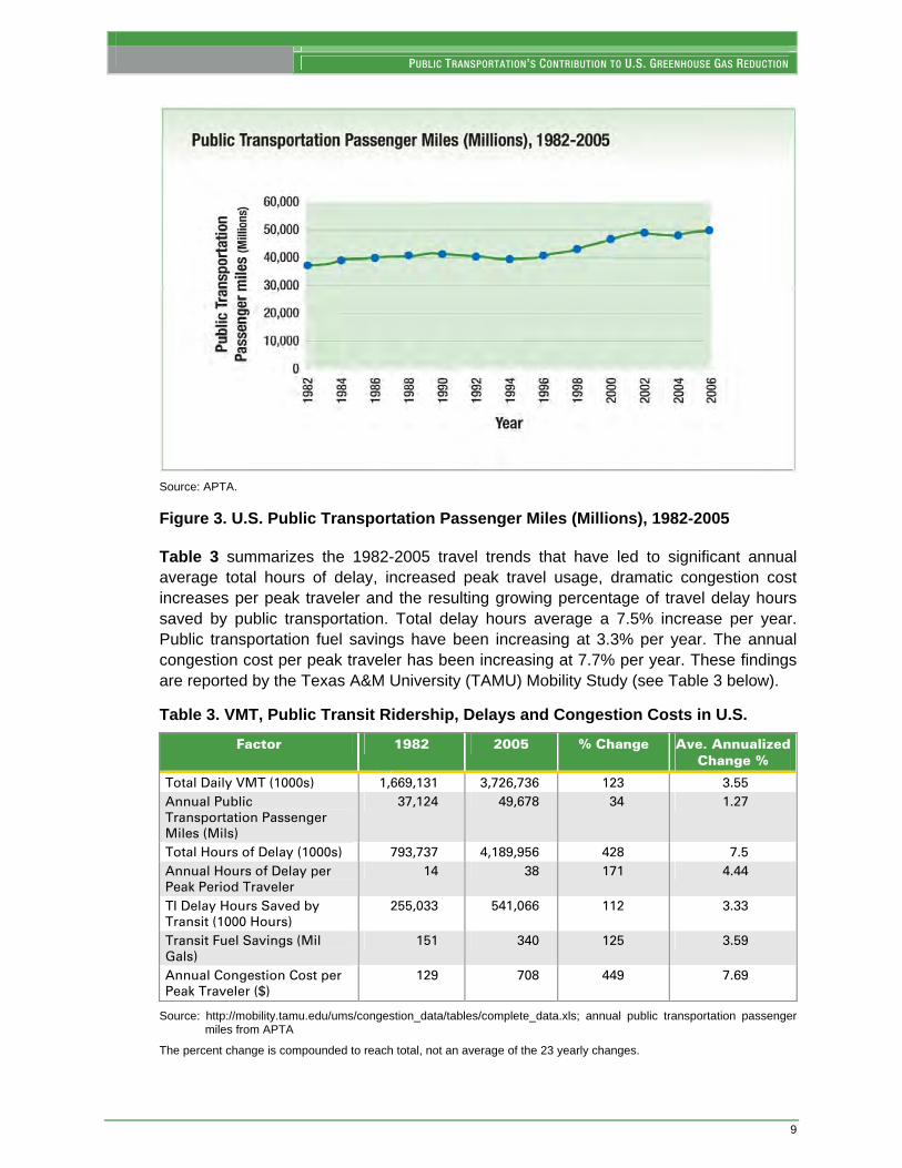
As shown in Figure 3, passenger miles of travel on public transportation have increased at an average annualized growth rate of 1.3% between 1982 and 2005. U.S. public transportation agencies have the capability to reduce foreign oil dependency and reduce CO2 emissions.


9

Source: APTA.

Figure 3. U.S. Public Transportation Passenger Miles (Millions), 1982-2005

Table 3 summarizes the 1982-2005 travel trends that have led to significant annual average total hours of delay, increased peak travel usage, dramatic congestion cost increases per peak traveler and the resulting growing percentage of travel delay hours saved by public transportation. Total delay hours average a 7.5% increase per year. Public transportation fuel savings have been increasing at 3.3% per year. The annual congestion cost per peak traveler has been increasing at 7.7% per year. These findings are reported by the Texas A&M University (TAMU) Mobility Study (see Table 3 below).

Table 3. VMT, Public Transit Ridership, Delays and Congestion Costs in U.S.

Factor 1982 2005 % Change Ave. Annualized Change %

Total Daily VMT (1000s) 1,669,131 3,726,736 123 3.55

Annual Public

Transportation Passenger

Miles (Mils)

37,124 49,678 34 1.27

Total Hours of Delay (1000s) 793,737 4,189,956 428 7.5

Annual Hours of Delay per

Peak Period Traveler

14 38 171 4.44

TI Delay Hours Saved by

Transit (1000 Hours)

255,033 541,066 112 3.33

Transit Fuel Savings (Mil

Gals)

151 340 125 3.59

Annual Congestion Cost per

Peak Traveler ($)

129 708 449 7.69

Source: http://mobility.tamu.edu/ums/congestion_data/tables/complete_data.xls; annual public transportation passenger miles from APTA

The percent change is compounded to reach total, not an average of the 23 yearly changes.


10

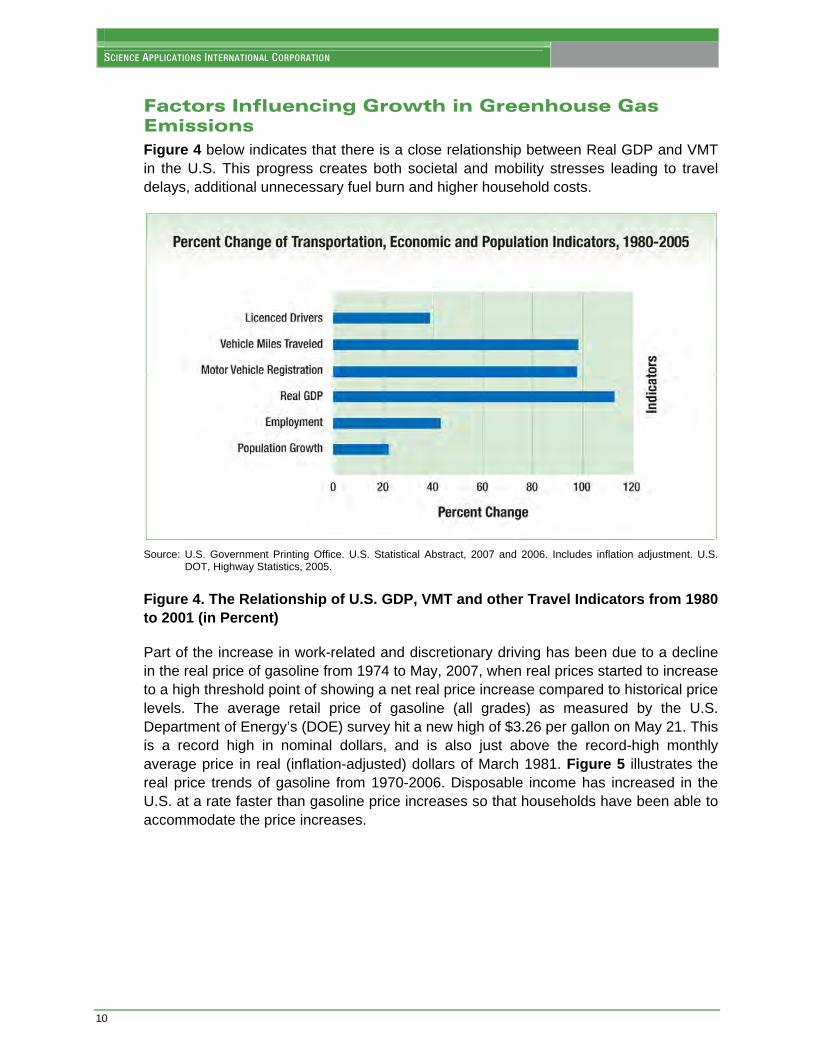
Factors Influencing Growth in Greenhouse Gas Emissions Figure 4 below indicates that there is a close relationship between Real GDP and VMT in the U.S. This progress creates both societal and mobility stresses leading to travel delays, additional unnecessary fuel burn and higher household costs.

Source: U.S. Government Printing Office. U.S. Statistical Abstract, 2007 and 2006. Includes inflation adjustment. U.S.

DOT, Highway Statistics, 2005.

Figure 4. The Relationship of U.S. GDP, VMT and other Travel Indicators from 1980 to 2001 (in Percent)

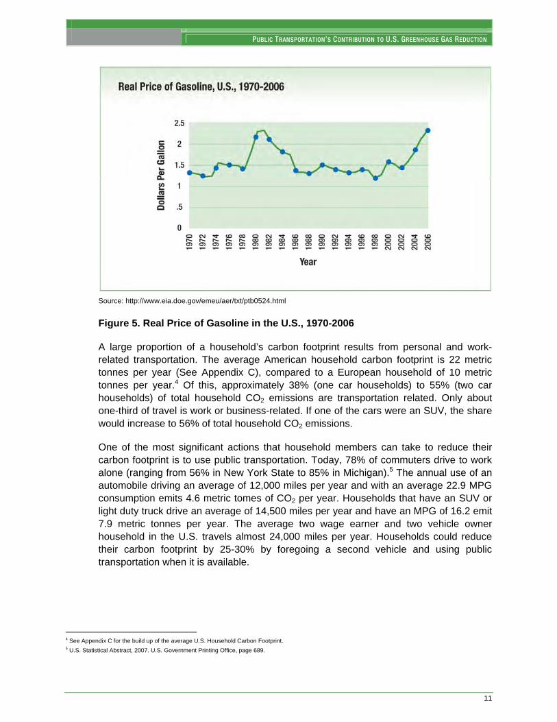
Part of the increase in work-related and discretionary driving has been due to a decline in the real price of gasoline from 1974 to May, 2007, when real prices started to increase to a high threshold point of showing a net real price increase compared to historical price levels. The average retail price of gasoline (all grades) as measured by the U.S. Department of Energy’s (DOE) survey hit a new high of $3.26 per gallon on May 21. This is a record high in nominal dollars, and is also just above the record-high monthly average price in real (inflation-adjusted) dollars of March 1981. Figure 5 illustrates the real price trends of gasoline from 1970-2006. Disposable income has increased in the U.S. at a rate faster than gasoline price increases so that households have been able to accommodate the price increases.


11

Source: http://www.eia.doe.gov/emeu/aer/txt/ptb0524.html

Figure 5. Real Price of Gasoline in the U.S., 1970-2006

A large proportion of a household’s carbon footprint results from personal and work-related transportation. The average American household carbon footprint is 22 metric tonnes per year (See Appendix C), compared to a European household of 10 metric tonnes per year.4 Of this, approximately 38% (one car households) to 55% (two car households) of total household CO2 emissions are transportation related. Only about one-third of travel is work or business-related. If one of the cars were an SUV, the share would increase to 56% of total household CO2 emissions.

One of the most significant actions that household members can take to reduce their carbon footprint is to use public transportation. Today, 78% of commuters drive to work alone (ranging from 56% in New York State to 85% in Michigan).5 The annual use of an automobile driving an average of 12,000 miles per year and with an average 22.9 MPG consumption emits 4.6 metric tomes of CO2 per year. Households that have an SUV or light duty truck drive an average of 14,500 miles per year and have an MPG of 16.2 emit 7.9 metric tonnes per year. The average two wage earner and two vehicle owner household in the U.S. travels almost 24,000 miles per year. Households could reduce their carbon footprint by 25-30% by foregoing a second vehicle and using public transportation when it is available.

4 See Appendix C for the build up of the average U.S. Household Carbon Footprint. 5 U.S. Statistical Abstract, 2007. U.S. Government Printing Office, page 689.


12

Potential Role of Public Transportation in Reducing CO2 Emissions Traveling by public transportation is less carbon intensive than traveling in a single occupant vehicle. Partially or more fully loaded buses and rail coaches are more environmentally friendly than lower occupancy single vehicles. A single person automobile traveling one mile emits on average 1.0 pounds of CO2.

SAIC evaluated the carbon footprint of the current U.S. transit industry and also investigated how much carbon mass transit ridership helps avoid. This analysis involved the following steps:

Personal vehicle use factors — Estimate the passenger miles for work and non-work related purposes in 2005 by car and

light duty vehicles — Estimate VMT by trip purpose and vehicle type — Take into account average occupancy factors — Estimate total household VMT and passenger miles by trip purpose

Calculate transit passenger miles by function and substituted passenger miles by function — A total of 49,678,000,000 miles were reported in the APTA 2007 Public Transportation

Fact Book. — The ratio of work and non-work travel miles are estimated and linked to vehicle mode and

occupancy levels — Calculate substitute gallons — Calculate substituted carbon

The energy and carbon footprint for the transit industry was calculated based on the 2007 Public Transportation Fact Book fuel volumes. — A standard coefficient of 1.341 pounds of carbon dioxide emissions was used for every

(kilowatt hour) kWh consumed by public transportation to arrive at a carbon footprint estimate. This is the 2000 emissions estimate suggested by DOE.6

— The total public transportation related carbon emissions were calculated — The direct substitution of transit for private vehicle travel saved was calculated and the

snapshot one year – 2005 net carbon savings from mass transit was calculated.

Assuming in 2005, if all travel that occurred on public transportation were to be completed instead in private vehicles, this would have resulted in an additional 16.2 million metric tonnes of carbon dioxide. Public transportation’s carbon emissions were 12.3 million metric tonnes, or 4.0 million metric tonnes less than would have been used by personal vehicles. In addition, the use of public transportation reduced congestion levels to the effect of saving an additional 340 million gallons of gasoline, which equated to another 3.0 million metric tonnes of CO2 reduction. This results in a net CO2 emission reduction of 6.9 million metric tonnes when the avoided congestion fuel consumption due is included. An additional 400,000 metric tonnes of additional GHGs were also saved, including sulfur hexafluoride, HFCs, perfluorocarbons, and chlorofluorocarbons.

6 Note: The actual carbon dioxide emissions for a transit system for each kWh consumed will vary by region and utility depending on the mix of primary energy

used to generate a kWh. EPA and DOE do report on the carbon content of electricity by state.


13

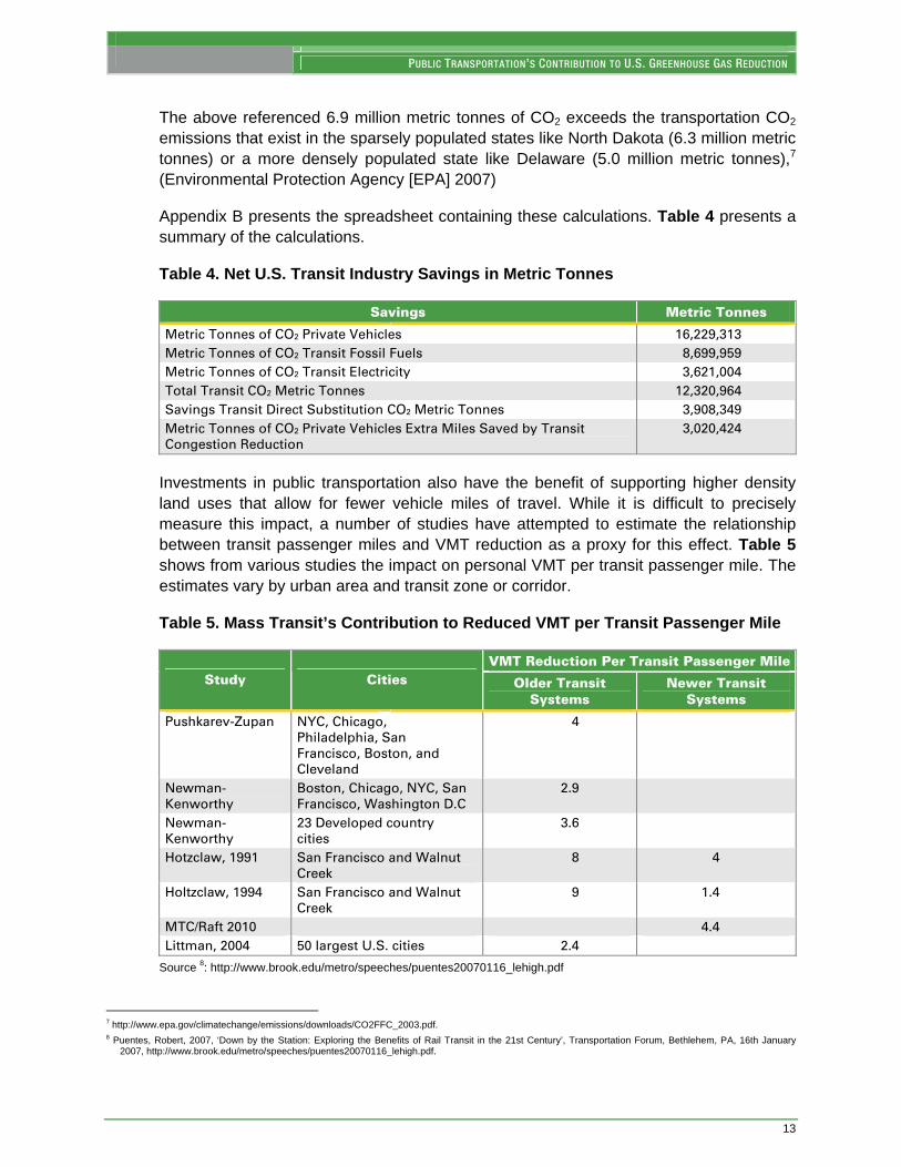
The above referenced 6.9 million metric tonnes of CO2 exceeds the transportation CO2 emissions that exist in the sparsely populated states like North Dakota (6.3 million metric tonnes) or a more densely populated state like Delaware (5.0 million metric tonnes),7 (Environmental Protection Agency [EPA] 2007)

Appendix B presents the spreadsheet containing these calculations. Table 4 presents a summary of the calculations.

Table 4. Net U.S. Transit Industry Savings in Metric Tonnes

Savings Metric Tonnes

Metric Tonnes of CO2 Private Vehicles 16,229,313

Metric Tonnes of CO2 Transit Fossil Fuels 8,699,959

Metric Tonnes of CO2 Transit Electricity 3,621,004

Total Transit CO2 Metric Tonnes 12,320,964

Savings Transit Direct Substitution CO2 Metric Tonnes 3,908,349

Metric Tonnes of CO2 Private Vehicles Extra Miles Saved by Transit

Congestion Reduction

3,020,424

Investments in public transportation also have the benefit of supporting higher density land uses that allow for fewer vehicle miles of travel. While it is difficult to precisely measure this impact, a number of studies have attempted to estimate the relationship between transit passenger miles and VMT reduction as a proxy for this effect. Table 5 shows from various studies the impact on personal VMT per transit passenger mile. The estimates vary by urban area and transit zone or corridor.

Table 5. Mass Transit’s Contribution to Reduced VMT per Transit Passenger Mile

VMT Reduction Per Transit Passenger MileStudy Cities Older Transit

Systems Newer Transit

Systems

Pushkarev-Zupan NYC, Chicago,

Philadelphia, San

Francisco, Boston, and

Cleveland

4

Newman-

Kenworthy

Boston, Chicago, NYC, San

Francisco, Washington D.C

2.9

Newman-

Kenworthy

23 Developed country

cities

3.6

Hotzclaw, 1991 San Francisco and Walnut

Creek

8 4

Holtzclaw, 1994 San Francisco and Walnut

Creek

9 1.4

MTC/Raft 2010 4.4

Littman, 2004 50 largest U.S. cities 2.4

Source 8: http://www.brook.edu/metro/speeches/puentes20070116_lehigh.pdf

7 http://www.epa.gov/climatechange/emissions/downloads/CO2FFC_2003.pdf. 8 Puentes, Robert, 2007, ‘Down by the Station: Exploring the Benefits of Rail Transit in the 21st Century’, Transportation Forum, Bethlehem, PA, 16th January

2007, http://www.brook.edu/metro/speeches/puentes20070116_lehigh.pdf.


14

GHG emissions from the U.S. transportation sector can be significantly lowered by converting vehicle miles of travel into transit passenger miles. Increasing rail or bus use is a practical method of reducing CO2 and traffic congestion. To optimize mass transit’s competitive advantages in terms of speed, convenience, and desirability, urban and suburban planning and design are required to encourage greater use of public transportation. There are a number of examples and case studies in public transportation of recent initiatives that have been successful in accomplishing this. Examples include the following:

The King County/Seattle/Metro Transit has embarked upon an ambitious “Transit Now” program to add 60,000 additional riders for Metro Transit buses. King County/Metro Transit’s use of bio-diesel is expected to remove an estimated 22,000 metric tons of carbon dioxide generated by transit vehicles in the coming year. That’s the equivalent of removing 2,800 vehicles from King County roadways. King County/Seattle/Metro Transit is a member of the Chicago Climate Exchange (CCX). This requires a commitment to reduce their carbon footprint by 6% from the base year for measuring emissions (1998-2001 CO2

emissions). The transit system in Grand Rapids increased work-related ridership from 48 to 61%

over the past 10+ years. In addition, Rapid Central Station in Downtown Grand Rapids, MI became the first transit facility to obtain basic Leadership in Energy and Environmental Design (LEED) certification status.9 The 51,000 square foot (SF), 21 bus transfer facility includes an undulating roof structure, recycled glass flooring, low E glass, and a roof garden system for added insulation.

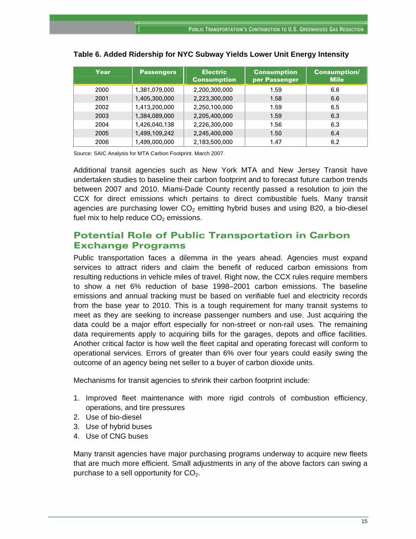
The New York Metropolitan Transportation Authority (MTA), New York City Transit has reported significant increases in subway ridership and a corresponding reduction in energy use per passenger miles traveled. MTA passenger ridership increased 8.5% on New York Subways from 2000 to 2006. Energy use declined 7.5% per passenger and 6% per mile as shown in Table 6. Also, with 100% of MTA Long Island Bus already converted to compressed natural gas (CNG), it is anticipated that limited growth of CO2 output will occur from 2000 to 2006. With fleet expansion and the conversion of buses from diesel to 100% CNG projected, CO2 emissions are expected to significantly decline by 2010. Finally, MTA NYC Transit expects to have up to 40% of its bus fleet converted to hybrid buses by 2010, further contributing to the decline in CO2 emissions.

9 U.S. Green Building Council, Leadership in Energy and Environmental Design Rating System. See: http://www.usgbc.org/ .


15

Table 6. Added Ridership for NYC Subway Yields Lower Unit Energy Intensity

Year Passengers Electric Consumption

Consumption per Passenger

Consumption/ Mile

2000 1,381,079,000 2,200,300,000 1.59 6.6

2001 1,405,300,000 2,223,300,000 1.58 6.6

2002 1,413,200,000 2,250,100,000 1.59 6.5

2003 1,384,089,000 2,205,400,000 1.59 6.3

2004 1,426,040,138 2,226,300,000 1.56 6.3

2005 1,499,109,242 2,245,400,000 1.50 6.4

2006 1,499,000,000 2,183,500,000 1.47 6.2

Source: SAIC Analysis for MTA Carbon Footprint. March 2007.

Additional transit agencies such as New York MTA and New Jersey Transit have undertaken studies to baseline their carbon footprint and to forecast future carbon trends between 2007 and 2010. Miami-Dade County recently passed a resolution to join the CCX for direct emissions which pertains to direct combustible fuels. Many transit agencies are purchasing lower CO2 emitting hybrid buses and using B20, a bio-diesel fuel mix to help reduce CO2 emissions.

Potential Role of Public Transportation in Carbon Exchange Programs Public transportation faces a dilemma in the years ahead. Agencies must expand services to attract riders and claim the benefit of reduced carbon emissions from resulting reductions in vehicle miles of travel. Right now, the CCX rules require members to show a net 6% reduction of base 1998–2001 carbon emissions. The baseline emissions and annual tracking must be based on verifiable fuel and electricity records from the base year to 2010. This is a tough requirement for many transit systems to meet as they are seeking to increase passenger numbers and use. Just acquiring the data could be a major effort especially for non-street or non-rail uses. The remaining data requirements apply to acquiring bills for the garages, depots and office facilities. Another critical factor is how well the fleet capital and operating forecast will conform to operational services. Errors of greater than 6% over four years could easily swing the outcome of an agency being net seller to a buyer of carbon dioxide units.

Mechanisms for transit agencies to shrink their carbon footprint include:

1. Improved fleet maintenance with more rigid controls of combustion efficiency, operations, and tire pressures

2. Use of bio-diesel 3. Use of hybrid buses 4. Use of CNG buses

Many transit agencies have major purchasing programs underway to acquire new fleets that are much more efficient. Small adjustments in any of the above factors can swing a purchase to a sell opportunity for CO2.


16

Some transit systems are considering membership into the CCX and are engaging in studies to evaluate what the cost exposure is for having to buy offsetting carbon credits should system expansion require purchases to be six percent below base 1998-2001 levels. Right now, the cost of CO2 in the U.S. is extremely low – about $0.03 per metric tonne.10 Often transit agencies will do their economic assessment on a $3.25/metric tonne implied value or even assume that carbon prices will increase to $10-30/metric tonne once the U.S. Government creates a system of cap and trade or a CO2 tax.

It is unclear what the future price of CO2 will be and how this should be factored into transit system financing and budgeting. But under the cap and trade programs currently underway in the U.S., the price of SO2 in 2005 was trading at $800 per ton and NOx in the Houston/Galveston area was trading at $40,000/ton. If the U.S. Government starts a cap and trade program and over time reduces the number of available allowances to meet carbon reduction targets, the value of carbon dioxide allowances will likely increase as it has for other regulated pollution sources.

A strategy is underway by some transit authorities to consider joining the CCX and possibly gain membership to the rules committee. This would help possibly influence a revision in rules that allows a public transportation agency to offset increases in their own carbon footprint by the ridership increases that occurred from a reduction of SOV use.

In addition, there may also be new policies that include tolling, permitting fees for entrance into central downtown zones, reduced parking, which could help stimulate additional public transportation use and GHG reductions. There may be occasions where even large local private employers will develop ridesharing programs using public transportation. In these cases, there will be a need to clarify how the carbon credits are split. With the U.S. Conference of Mayors supporting local climate change and with many state governments implementing green energy purchasing and climate programs of their own, private carbon exchanges will need to acknowledge the potential significance of these programs and work to allow offsets for public transportation expansion and the benefits of regional urban CO2 reductions.

10 Actual price is $3.30 per CFI which is 100 metric tonnes. Dividing $3.30 by 100 is three cents. This compares to 22.16 Euros/metric tonne which is $30.39 per

metric tonne.


17

Bibliography

American Public Transportation Association (2007) On Public Transportation, Energy Independence and Climate Change: House Committee On Transportation And Infrastructure Testimony Of William W. Millar, President, American Public Transportation Association Submitted To The House Committee On Transportation And Infrastructure On Public Transportation, Energy Independence and Climate Change, May 16, 2007, http://www.apta.com/government_affairs/aptatest/documents/testimony070516.pdf

American Public Transportation Association (2007) House and Senate Members on Energy and Climate Change Legislation, May 3, 2007, http://www.apta.com/government_affairs/letters/documents/070503baucus.pdf

Canadian Urban Transit Association (CUTA), Public Transit: A Climate Change Solution, CUTA Issue Paper No. 16, http://www.cutaactu.ca/sites/cutaactu.ca/files/IssuePaper16E.pdf

Evans, Meredydd, Transportation in Transition Economies: a Key to Carbon Management, Pacific Northwest National Laboratory (Panel V, 16 – Evans), http://www.pnl.gov/aisu/pubs/transcmgt.pdf

EPA A Wedge Analysis of the U.S. Transportation Sector Report: (23 pp, 535K, EPA420-R-07-007, April 2007), http://www.epa.gov/otaq/climate/420r07007.pdf

EPA Greenhouse Gas Emissions from the U.S. Transportation Sector: 1990-2003 (EPA420-R-06-003, March 2006), (68 pp, 1.2MB) http://www.epa.gov/otaq/climate/420r06003.pdf

EPA Emission Facts: Average Carbon Dioxide Emissions Resulting from Gasoline and Diesel Fuel Fact Sheet: (3 pages, 29K, EPA420-F-05-001, February 2005), http://www.epa.gov/otaq/climate/420f05003.pdf

EPA Emission Facts: Metrics for Expressing Greenhouse Gas Emissions: Carbon Equivalents and Carbon Dioxide Equivalents Fact Sheet: (3 pp, 35K, EPA420-F-05-002, February 2005) http://www.epa.gov/otaq/climate/420f05002.pdf

EPA Emission Facts: Calculating Emissions of Greenhouse Gases: Key Facts and Figures Fact Sheet: (5 pp, 45K, EPA420-F-05-003, February 2005) http://www.epa.gov/otaq/climate/420f05003.pdf

EPA Emission Facts: Greenhouse Gas Emissions from a Typical Passenger Vehicle Fact Sheet: (6 pp, 54K, EPA420-F-05-004, February 2005) http://www.epa.gov/otaq/climate/420f05004.pdf

EPA Update of Methane and Nitrous Oxide Emission Factors for On-Highway Vehicles Report (39 pp, 683K, EPA420-P-04-016, November 2004)


18

EPA Light-Duty Automotive Technology and Fuel Economy Trends: 1975 Through 2005 Report (90 pp, 3.8MB, EPA420-R-05-001, July 2005)

EPA Emissions of Nitrous Oxide from Highway Mobile Sources: Comments on the Draft Inventory of U.S. Greenhouse Gas Emissions and Sinks, 1990-1996 Report (March 1998) (38 pp, 139K, EPA420-R-98-009, August 1998)

FHWA (2004) Transportation and Air Quality Trends, 4/19/04: http://planning.transportation.org/sites/planning/docs/planning%20mon/Transportation%20and%20Air%20Quality%20Trends.pdf

Government of Canada (2005), Moving Forward on Climate Change: A Plan for honoring our Kyoto Commitment, 2005: www.climatechange.gc.ca

Lash, Jonathan (2007) Statement to the, U.S. House of Representatives Committee on Transportation and Infrastructure, May 16, 2007, http://pdf.wri.org/070516_lash_testimony.pdf

Transport Canada (2001) National Vision for Urban Transit to 2020, http://www.hwcn.org/link/tlc/TC_vision.pdf

Transport Canada, (2004) Fuel Sense: Making Fleet and Transit Operations More Efficient, Urban Transportation Showcase Program Case Study 24, www.tc.gc.ca/utsp

TRB Transit Cooperative Research Program (TCRP) (2003) Mitigating Climate Change with Sustainable Surface Transportation Report 93: Travel Matters http://onlinepubs.trb.org/onlinepubs/tcrp/tcrp_rpt_93.pdf

United States Department of Energy (2000), Natural Gas Buses: Separating Myth From Fact, www.eere.energy.gov


19

Appendix A

Background to Climate Change In February 2007, the Intergovernmental Panel on Climate Change (IPCC) reported that the current atmospheric concentration of CO2 and methane (two of the most significant GHGs) “exceeds by far the natural range over the last 650,000 years”. The majority of the climate scientific community believes a concerted and coordinated effort must be made to limit global warming to no more than 2 degrees Celsius above current levels to avoid the worst impacts of climate change. To limit global warming to less than 2 degrees Celsius, it is thought that atmospheric CO2 concentrations must not exceed 450-500 parts per million (ppm) (the current level is around 380 ppm and rising at more than 2 ppm per year). To achieve this, global emissions need to decrease dramatically during this century, perhaps on the order of 60 to 80 percent below current levels by 2050.

The IPCC projects that in 2039, average temperatures across North America will rise by 1.8 to 5.4 degrees Fahrenheit. Half the U.S. population (~150 million) lives in coastal communities and with sea levels rising off the U.S. coast at a rate of .08-.12 inches per year, these communities are at risk.

Worldwide emissions of GHGs have risen steeply during the past 60 years. About 42,000 megatonnes of CO2 were released into the atmosphere in 2000 (most recent data available). Global emissions of all GHGs rose by 7.5% during 1990–2000. Electricity and heat represent 25% of total global emissions, with land use change and forestry the second source at 18% globally. In terms of economic activity, road transport was responsible for nearly 10% of global emissions.

The GHG Issue Many forms of transportation create GHG (including CO2) emissions, both direct and indirect. Given that personal mobility is a pre-requisite of economic and modern life the question arises how to meet the mobility needs of a contemporary lifestyle and yet reduce direct and indirect emissions of GHGs.

Some GHGs such as CO2 occur naturally and are emitted to the atmosphere through natural processes and human activities. Other GHGs (e.g., fluorinated gases) are created by human activities.


20

Principal GHGs:

Carbon Dioxide (CO2)—Carbon dioxide enters the atmosphere through the burning of

fossil fuels (oil, natural gas, and coal), solid waste, trees and wood products, and also as a

result of other chemical reactions (e.g., manufacture of cement). Carbon dioxide is also

removed from the atmosphere (or “sequestered”) when it is absorbed by plants as part of

the biological carbon cycle.

Methane (CH4)—Methane is emitted during the production and transport of coal, natural

gas, and oil. Methane emissions also result from livestock and other agricultural practices

and by the decay of organic waste in municipal solid waste landfills.

Nitrous Oxide (N2O)—Nitrous oxide is emitted during agricultural and industrial activities,

as well as during combustion of fossil fuels and solid waste.

Fluorinated Gases—HFCs, perfluorocarbons, and sulfur hexafluoride are synthetic,

powerful GHGs that are emitted from a variety of industrial processes. Fluorinated gases are

sometimes used as substitutes for ozone-depleting substances (i.e., CFCs, HFCs, and halons).

Ozone—In the troposphere, it is a chemical oxidant, a GHG, and a major component of

photochemical smog. Ozone precursors are chemical compounds, such as carbon

monoxide, methane, non-methane hydrocarbons, and nitrogen oxides, which in the

presence of solar radiation react with other chemical compounds to form ozone.

These gases are typically emitted in smaller quantities, but because they are potent GHGs,

they are sometimes referred to as high global warming potential (GWP) gases (“high GWP

gases”).

Trading Carbon on the Chicago Climate Exchange Carbon Trading provides flexibility to meet a global problem and find least-cost means of reducing emissions The CCX is a self-regulatory organization overseen by Committees comprised of Exchange Members, directors and staff. The CCX has a number of Committees responsible for developing the CCX ‘Rules’ that include: Environmental Compliance, Forestry, Membership, Offsets, Trading and Market Operations.

The CCX offers a voluntary, integrated GHG reduction and trading system for all six GHGs, with offset projects in North America and globally that harnesses capital markets. The CCX operates the main carbon trading platform in the U.S. and the European Carbon Exchange. Participants pay an annual membership fee to the CCX which gives them the right to accumulate and trade carbon credits (in the form of Carbon Finance Instrument [CFI] units). CCX participants sign on to specific carbon emission reductions.

The practical and strategic drivers of CCX participation include:

First-mover advantage and building global linkages Getting ahead of the currently disparate regulations and prepare for inevitable

national policy and regulations Reduce long-term mitigation costs Build carbon price into decision-making of operators and planners Trading profits, possible early action crediting.

The carbon market architecture includes the following: Phase I: Members made legally binding commitments to reduce or trade 1% per year

from 2003-2006, for a total of 4% below baseline. The baseline is the average emissions from 1998-2001, emissions in 2000 (Phase II)


21

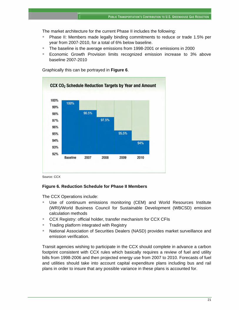
The market architecture for the current Phase II includes the following: Phase II: Members made legally binding commitments to reduce or trade 1.5% per

year from 2007-2010, for a total of 6% below baseline. The baseline is the average emissions from 1998-2001 or emissions in 2000 Economic Growth Provision limits recognized emission increase to 3% above

baseline 2007-2010

Graphically this can be portrayed in Figure 6.

Source: CCX

Figure 6. Reduction Schedule for Phase II Members

The CCX Operations include: Use of continuum emissions monitoring (CEM) and World Resources Institute

(WRI)/World Business Council for Sustainable Development (WBCSD) emission calculation methods

CCX Registry: official holder, transfer mechanism for CCX CFIs Trading platform integrated with Registry National Association of Securities Dealers (NASD) provides market surveillance and

emission verification.

Transit agencies wishing to participate in the CCX should complete in advance a carbon footprint consistent with CCX rules which basically requires a review of fuel and utility bills from 1998-2006 and then projected energy use from 2007 to 2010. Forecasts of fuel and utilities should take into account capital expenditure plans including bus and rail plans in order to insure that any possible variance in these plans is accounted for.


22

Issues Related to Transit’s Participation in Carbon Trading Public transportation must deal with a number of contending issues related to positioning itself to take advantage of, and limiting its risks associated with, the drive to reduce the carbon footprint of transit systems, divisions and how they apply to urban transportation congestion in major urban regions:

1. Expansion of routes and passenger volumes often lead to higher absolute energy use even though the emissions per passenger or car mile may decline.

2. Transit agencies operate in a larger area carbon footprint that contains other substantial emissions from manufacturers, businesses and other modes of transportation. Urban mass transit could cost effectively help reduce a regional areas carbon footprint but unfortunately experience a growth in its own carbon footprint.

3. Urban transit agencies comprise many different segments of businesses such as intercity rail, regional rail or light rail, urban bus operations, and para transit. Each of these business areas has their own historical and projected carbon footprint. To develop a strategy it is critical to know how different areas of operations contribute to growth or decline in the agency’s carbon footprint. Depending on the type of governance of a transit agency, there may be an opportunity to enroll a segment of the transportation authority rather than the entire agency if it is more likely that an agency will meet CCX carbon reduction requirements.

4. One of the challenging elements of creating a carbon footprint is to determine the carbon baseline back to 1998 or use a single year of 2000 and to report the annual historic energy consumption volumes for each year to 2006 and develop a reliable and valid forecast for 2007–2010. It is also important to obtain the build up data associated with fuel forecasts including fleet change out rates, MPG rates and passenger carrying forecasts.

5. Key factors that can alter a forecast are the train and bus fleet operational plan, capital plan and significant changes in traction and non-traction operational projects.

6. The CCX is seeking urban transit agency membership. For membership, the CCX is going to encourage agency participation on the rules committee. This involvement will provide an opportunity to provide input on future rule changes related to transit industry operations. Such participation will not have an immediate impact on some rule provisions like an absolute reduction on agency fuel use and carbon emissions. However, CCX says that participating on the rule committee could help make changes on future rule. The current rules require that all combustible fuels including fleet fuel and energy use and other ancillary combustible fuels be accounted for. This may be difficult to acquire.


23

7. The cost effectiveness of transit’s participation in the CCX may rest on the determination of the net increase or reduction in carbon offsets or purchases on an annualized basis over the 2007–2010 time period. Factors to include in this assessment are: The cost or value of the carbon units purchased or saved respectively, Benefits that possibly accrue to the larger carbon pool in the region that the

transit agency can claim, The operational and capital costs and savings associated with fleet operations.

8. There is no standard methodology developed to value these additional cost effective factors.

Public transportation needs to assess the potential benefits and risks in joining the CCX as it now stands and how the rules need to change to better reflect the net benefits of increasing transit ridership as a means to cutting GHGs.


24



25

Appendix B

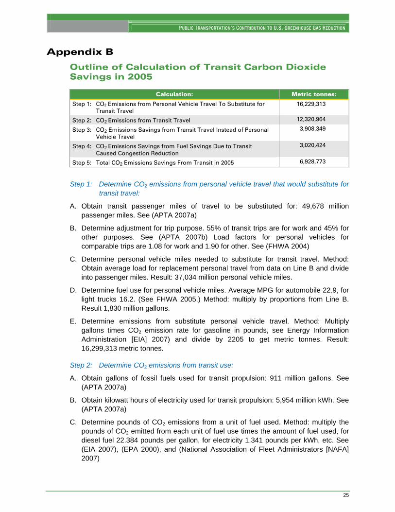
Outline of Calculation of Transit Carbon Dioxide Savings in 2005

Calculation: Metric tonnes:

Step 1: CO2 Emissions from Personal Vehicle Travel To Substitute for

Transit Travel

16,229,313

Step 2: CO2 Emissions from Transit Travel 12,320,964

Step 3: CO2 Emissions Savings from Transit Travel Instead of Personal

Vehicle Travel

3,908,349

Step 4: CO2 Emissions Savings from Fuel Savings Due to Transit

Caused Congestion Reduction

3,020,424

Step 5: Total CO2 Emissions Savings From Transit in 2005 6,928,773

Step 1: Determine CO2 emissions from personal vehicle travel that would substitute for transit travel:

A. Obtain transit passenger miles of travel to be substituted for: 49,678 million passenger miles. See (APTA 2007a)

B. Determine adjustment for trip purpose. 55% of transit trips are for work and 45% for other purposes. See (APTA 2007b) Load factors for personal vehicles for comparable trips are 1.08 for work and 1.90 for other. See (FHWA 2004)

C. Determine personal vehicle miles needed to substitute for transit travel. Method: Obtain average load for replacement personal travel from data on Line B and divide into passenger miles. Result: 37,034 million personal vehicle miles.

D. Determine fuel use for personal vehicle miles. Average MPG for automobile 22.9, for light trucks 16.2. (See FHWA 2005.) Method: multiply by proportions from Line B. Result 1,830 million gallons.

E. Determine emissions from substitute personal vehicle travel. Method: Multiply gallons times CO2 emission rate for gasoline in pounds, see Energy Information Administration [EIA] 2007) and divide by 2205 to get metric tonnes. Result: 16,299,313 metric tonnes.

Step 2: Determine CO2 emissions from transit use:

A. Obtain gallons of fossil fuels used for transit propulsion: 911 million gallons. See (APTA 2007a)

B. Obtain kilowatt hours of electricity used for transit propulsion: 5,954 million kWh. See (APTA 2007a)

C. Determine pounds of CO2 emissions from a unit of fuel used. Method: multiply the pounds of CO2 emitted from each unit of fuel use times the amount of fuel used, for diesel fuel 22.384 pounds per gallon, for electricity 1.341 pounds per kWh, etc. See (EIA 2007), (EPA 2000), and (National Association of Fleet Administrators [NAFA] 2007)


26

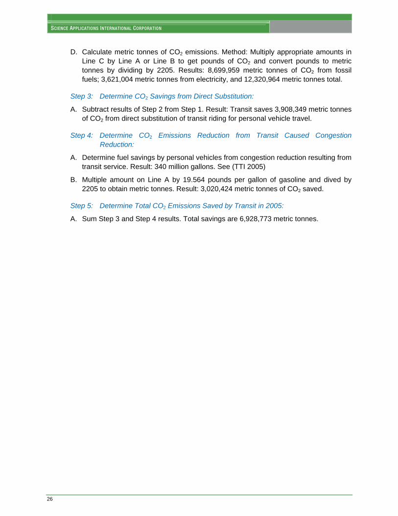
D. Calculate metric tonnes of CO2 emissions. Method: Multiply appropriate amounts in Line C by Line A or Line B to get pounds of CO2 and convert pounds to metric tonnes by dividing by 2205. Results: 8,699,959 metric tonnes of CO2 from fossil fuels; 3,621,004 metric tonnes from electricity, and 12,320,964 metric tonnes total.

Step 3: Determine CO2 Savings from Direct Substitution:

A. Subtract results of Step 2 from Step 1. Result: Transit saves 3,908,349 metric tonnes of CO2 from direct substitution of transit riding for personal vehicle travel.

Step 4: Determine CO2 Emissions Reduction from Transit Caused Congestion Reduction:

A. Determine fuel savings by personal vehicles from congestion reduction resulting from transit service. Result: 340 million gallons. See (TTI 2005)

B. Multiple amount on Line A by 19.564 pounds per gallon of gasoline and dived by 2205 to obtain metric tonnes. Result: 3,020,424 metric tonnes of CO2 saved.

Step 5: Determine Total CO2 Emissions Saved by Transit in 2005:

A. Sum Step 3 and Step 4 results. Total savings are 6,928,773 metric tonnes.


27

References APTA 2007a 2007 Public Transportation Fact Book. Washington: American Public Transportation Association, May 2007.

APTA 2007b A Profile of Public Transportation Passenger Demographics and Travel Characteristics Reported in On-Board Surveys. Washington: American Public Transit Association, May 2007.

EIA 2007 Voluntary Reporting of Greenhouse Gases Program Fuel and Energy Source Codes and Calculations. Washington: Energy Information Administration.

EPA 2000 Carbon Dioxide Emissions from the Generation of Electric Power in the United States. Washington: Environmental Protection Agency, 2000.

FHWA 2005 Highway Statistics 2005. Washington: Federal Highway Administration, 2005.

FHWA 2004 Hu, Patricia S. and Timothy R. Reuscher, Summary of Travel Trends 2001 National Household Travel Survey. Washington; Federal Highway Administration, December 2004.

NAFA 2007 Energy Equivalents of Various Fuels. Princeton, NJ: National Association of Fleet Administrators.

TTI 2005 2005 Annual Urban Mobility Report. College Station, TX: Texas Transportation Institute/Texas A&M University, 2005.

Source for CO2 emissions per 1 kWh. http://www.eia.doe.gov/cneaf/electricity/page/ CO2_report/ C02report.html#factors


28



29

Appendix C

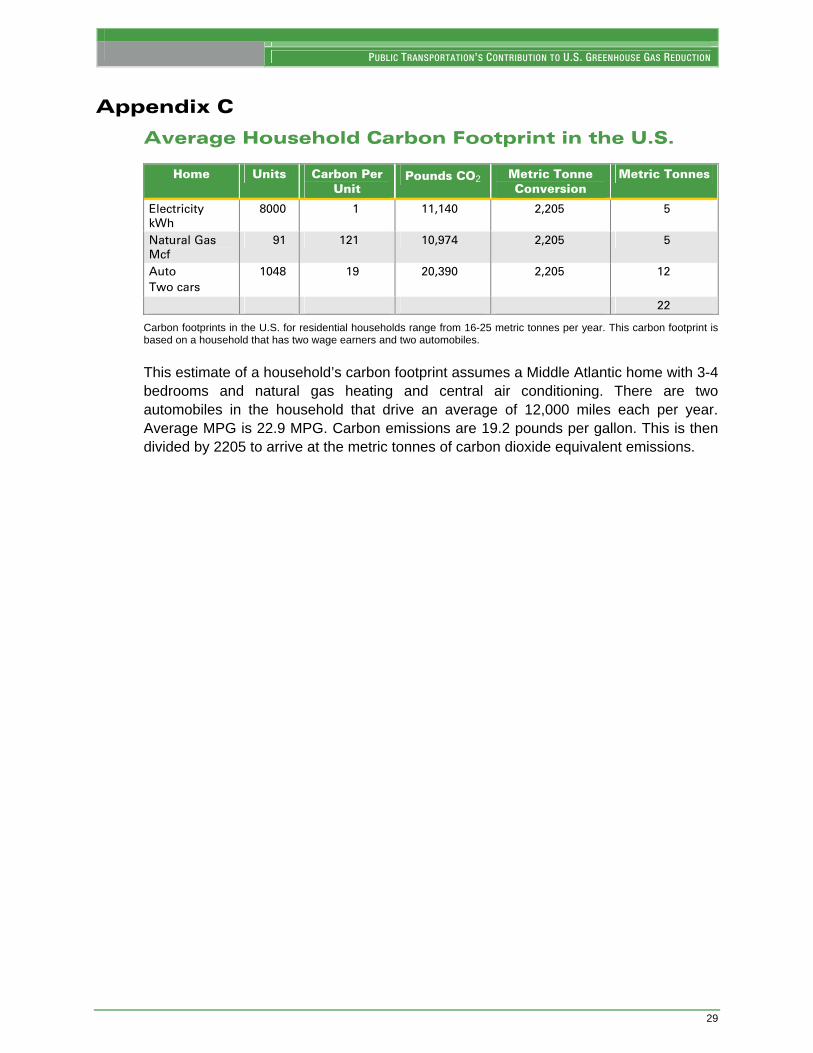
Average Household Carbon Footprint in the U.S.

Home Units Carbon Per Unit

Pounds CO2 Metric Tonne Conversion

Metric Tonnes

Electricity

kWh

8000 1 11,140 2,205 5

Natural Gas

Mcf

91 121 10,974 2,205 5

Auto

Two cars

1048 19 20,390 2,205 12

22

Carbon footprints in the U.S. for residential households range from 16-25 metric tonnes per year. This carbon footprint is based on a household that has two wage earners and two automobiles.

This estimate of a household’s carbon footprint assumes a Middle Atlantic home with 3-4 bedrooms and natural gas heating and central air conditioning. There are two automobiles in the household that drive an average of 12,000 miles each per year. Average MPG is 22.9 MPG. Carbon emissions are 19.2 pounds per gallon. This is then divided by 2205 to arrive at the metric tonnes of carbon dioxide equivalent emissions.


30



31

Appendix D

Measures and Metrics Carbon Dioxide (CO2): CO2 is the reference of comparison of all GHGs.

Carbon Dioxide Equivalent (CDE): A metric measure used to compare the emissions from GHGs based on their GWP. Carbon dioxide equivalents are usually expressed as “million metric tons of carbon dioxide equivalents (MMTCDE)” or “million short tons of carbon dioxide equivalents (MSTCDE)”.

Carbon dioxide equivalent for a gas is determined by multiplying the tons of the gas by the associated GWP. MMTCDE= (million metric tons of a gas) * (GWP of the gas).

For example, GWP for methane is 24.5, i.e., emissions of one million metric tons of methane is equivalent to emissions of 24.5 million metric tons of carbon dioxide. Carbon is used as the reference with other GHGs converted to carbon equivalents.

Conversion of carbon to carbon dioxide is achieved by multiplying carbon by 44/12 (the ratio of the molecular weight of carbon dioxide to carbon). (EPA).

Carbon Equivalent (CE) is a metric measure used to compare the emissions of GHGs based on their GWP. GHG emissions in the U.S. are commonly expressed as “million metric tons of carbon equivalents” (MMTCE). GWPs are used to convert GHGs to carbon dioxide equivalents. Carbon dioxide equivalents are converted to carbon equivalents by multiplying the carbon dioxide equivalents by 12/44 (the ratio of the molecular weight of carbon to carbon dioxide). The formula to derive carbon equivalents is: MMTCE = (million metric tons of a gas) * (GWP of the gas) * (12/44) (EPA).

Documents

Public Transportation's Contribution to US Greenhouse Gas Reduction