Embed Size (px)
Citation preview

Public Economics LecturesTaxes and Behavior: Labor Markets
John Karl Scholz (working from slides of Raj Chetty and Gregory A.Bruich)
University of Wisconsin —MadisonFall 2011
JK Scholz ()Tax Incentives and Saving 1 / 69

Brief Discussion of Theoretical Issues in Labor SupplyEstimation
Labor supply elasticity is a parameter of fundamental importance forincome tax policy
Optimal tax rate depends inversely on εc = ∂ log l∂ logw U=U
, thecompensated wage elasticity of labor supply
First discuss econometric issues that arise in estimating εc
We’ll just discuss the baseline model: (1) static, (2) linear tax system,(3) pure intensive margin choice, (4) single hours choice, (5) nofrictions
JK Scholz ()Tax Incentives and Saving 2 / 69

Static Model: Setup
Let c denote consumption and l hours worked
Normalize price of c to one
Agent has utility u(c , l) = c − a l1+1/ε
1+1/ε
Agent earns wage w per hour worked and has y in non-labor income
With tax rate τ on labor income, individual solves
max u(c, l) s.t. c = (1− τ)wl + y
JK Scholz ()Tax Incentives and Saving 3 / 69

Labor Supply Behavior
First order condition(1− τ)w = al1/ε
Yields labor supply function
l = α+ ε log(1− τ)w
Here y does not matter because u is quasilinear
Log-linearization of general utility u(c , l) would yield a labor supply fnof the form:
l = α+ ε log(1− τ)w − ηy
Can recover εc from ε and η using Slutsky equation
JK Scholz ()Tax Incentives and Saving 4 / 69
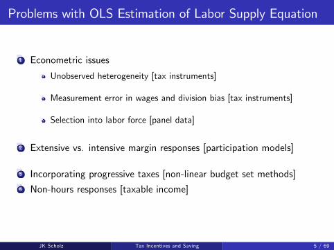
Problems with OLS Estimation of Labor Supply Equation
1 Econometric issues
Unobserved heterogeneity [tax instruments]
Measurement error in wages and division bias [tax instruments]
Selection into labor force [panel data]
2 Extensive vs. intensive margin responses [participation models]
3 Incorporating progressive taxes [non-linear budget set methods]4 Non-hours responses [taxable income]
JK Scholz ()Tax Incentives and Saving 5 / 69

Econometric Problem 1: Unobserved Heterogeneity
Early studies estimated elasticity using cross-sectional variation inwage rates
Problem: unobserved heterogeneity
Those with high wages also have a high propensity to work
Cross-sectional correlation between w and h likely to yield an upwardbiased estimate of ε
Solution: use taxes as instruments for (1− τ)w
JK Scholz ()Tax Incentives and Saving 6 / 69
Econometric Problem 2: Measurement Error/Division Bias
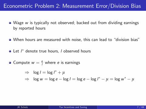
Wage w is typically not observed; backed out from dividing earningsby reported hours
When hours are measured with noise, this can lead to “division bias”
Let l∗ denote true hours, l observed hours
Compute w = el where e is earnings
⇒ log l = log l∗ + µ
⇒ logw = log e − log l = log e − log l∗ − µ = logw ∗ − µ
JK Scholz ()Tax Incentives and Saving 7 / 69

Measurement Error and Division Bias
Mis-measurement of hours causes a spurious link between hours andwages
Estimate a regression of the following form:
log l = β1 + β2 logw + ε
Then
E β2 =cov(log l , logw)var(logw)
=cov(log l∗ + µ, logw ∗ − µ)
var(logw) + var(µ)
Problem: E β2 6= ε because orthogonality restriction for OLS violated
Ex. workers with high mis-reported hours also have low imputedwages, biasing elasticity estimate downward
Solution: tax instruments again
JK Scholz ()Tax Incentives and Saving 8 / 69

Econometric Problem 3: Selection into Labor Force
Consider model with fixed costs of working, where some individualschoose not to work
Wages are unobserved for non-labor force participants
Thus, OLS regression on workers only includes observations withli > 0
This can bias OLS estimates: low wage earners must have very highunobserved propensity to work to find it worthwhile
Requires a selection correction (e.g. Heckit, Tobit, or ML estimation)
See Killingsworth and Heckman (1986) for implementation
Current approach: use panel data to distinguish entry/exit fromintensive-margin changes
JK Scholz ()Tax Incentives and Saving 9 / 69
Extensive vs. Intensive Margin
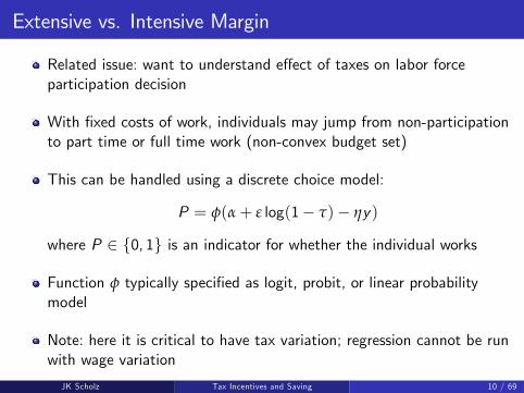
Related issue: want to understand effect of taxes on labor forceparticipation decision
With fixed costs of work, individuals may jump from non-participationto part time or full time work (non-convex budget set)
This can be handled using a discrete choice model:
P = φ(α+ ε log(1− τ)− ηy)
where P ∈ {0, 1} is an indicator for whether the individual works
Function φ typically specified as logit, probit, or linear probabilitymodel
Note: here it is critical to have tax variation; regression cannot be runwith wage variation
JK Scholz ()Tax Incentives and Saving 10 / 69

A (lengthy) Digression: Progressive Taxes and LaborSupply
OLS regression specification is derived from model with a single lineartax rate
In practice, income tax systems are non-linear
Consider effect of US income tax code on budget sets
JK Scholz ()Tax Incentives and Saving 11 / 69

Source: Congressional Budget Offi ce 2005
JK Scholz ()Tax Incentives and Saving 12 / 69

Example 1: Progressive Income Tax
JK Scholz ()Tax Incentives and Saving 13 / 69

Example 2: EITC
JK Scholz ()Tax Incentives and Saving 14 / 69

Example 3: Social Security Payroll Tax Cap
JK Scholz ()Tax Incentives and Saving 15 / 69

Example 4: Negative Income Tax
JK Scholz ()Tax Incentives and Saving 16 / 69

Progressive Taxes and Labor Supply
Non-linear budget set creates two problems:
1 Model mis-specification: OLS regression no longer recovers structuralelasticity parameter ε of interest
Two reasons: (1) underestimate response because people pile up atkink and (2) mis-estimate income effects
2 Econometric bias: τi depends on income wi li and hence on li
Tastes for work are positively correlated with τi → downward bias inOLS regression of hours worked on net-of-tax rates
Solution to problem #2: only use reform-based variation in tax rates
But problem #1 requires fundamentally different estimation method
JK Scholz ()Tax Incentives and Saving 17 / 69

Hausman: Non-linear Budget Constraints
Hausman pioneered structural approach to estimating elasticities withnon-linear budget sets
Assume an uncompensated labor supply equation:
l = α+ βw(1− τ) + γy + ε
Error term ε is normally distributed with variance σ2
Observed variables: wi , τi , yi , and li
Technique: (1) construct likelihood function given observed laborsupply choices on NLBS, (2) find parameters (α, β,γ) that maximizelikelihood
Important insight: need to use “virtual incomes” in lieu of actualunearned income with NLBS
JK Scholz ()Tax Incentives and Saving 18 / 69

Non-Linear Budget Set Estimation: Virtual Incomes
S ource: Hausman 1985
L1L2 l*L
$
y1
y2
y3
w3
w2
w1
JK Scholz ()Tax Incentives and Saving 19 / 69

NLBS Likelihood Function
Consider a two-bracket tax system
Individual can locate on first bracket, on second bracket, or at thekink lK
Likelihood = probability that we see individual i at labor supply ligiven a parameter vector
Decompose likelihood into three components
Component 1: individual i on first bracket: 0 < li < lK
li = α+ βwi (1− τ1) + γy1 + εi
Error εi = li − (α+ βwi (1− τ1) + γy1). Likelihood:
Li = φ((li − (α+ βwi (1− τ1) + γy1)/σ)
Component 2: individual i on second bracket: lK < li . Likelihood:
Li = φ((li − (α+ βwi (1− τ2) + γy2)/σ)
JK Scholz ()Tax Incentives and Saving 20 / 69
Likelihood Function: Located at the Kink
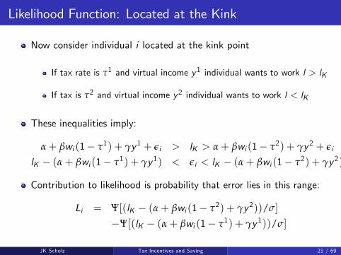
Now consider individual i located at the kink point
If tax rate is τ1 and virtual income y1 individual wants to work l > lK
If tax is τ2 and virtual income y2 individual wants to work l < lK
These inequalities imply:
α+ βwi (1− τ1) + γy1 + εi > lK > α+ βwi (1− τ2) + γy2 + εi
lK − (α+ βwi (1− τ1) + γy1) < εi < lK − (α+ βwi (1− τ2) + γy2)
Contribution to likelihood is probability that error lies in this range:
Li = Ψ[(lK − (α+ βwi (1− τ2) + γy2))/σ]
−Ψ[(lK − (α+ βwi (1− τ1) + γy1))/σ]
JK Scholz ()Tax Incentives and Saving 21 / 69
Maximum Likelihood Estimation
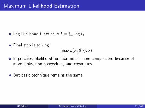
Log likelihood function is L = ∑i log Li
Final step is solvingmax L(α, β,γ, σ)
In practice, likelihood function much more complicated because ofmore kinks, non-convexities, and covariates
But basic technique remains the same
JK Scholz ()Tax Incentives and Saving 22 / 69

Hausman (1981) Application
Hausman applies method to 1975 PSID cross-section
Finds significant compensated elasticities and large income effects
Elasticities larger for women than for men
Shortcomings of this implementation
1 Sensitivity to functional form choices, which is a larger issue withstructural estimation
2 No tax reforms, so does not solve fundamental econometric problemthat tastes for work may be correlated with w
JK Scholz ()Tax Incentives and Saving 23 / 69

NLBS and Bunching at Kinks
Subsequent studies obtain different estimates (MaCurdy, Green, andPaarsh 1990, Blomquist 1995)
Several studies find negative compensated wage elasticity estimates
Debate: impose requirement that compensated elasticity is positive orconclude that data rejects model?
Fundamental source of problem: labor supply model predicts thatindividuals should bunch at the kink points of the tax schedule
But we observe very little bunching at kinks, so model is rejected bythe data
Interest in NLBS models diminished despite their conceptualadvantages over OLS methods
JK Scholz ()Tax Incentives and Saving 24 / 69

Saez 2009: Bunching at Kinks
Saez observes that only non-parametric source of identification forelasticity in a cross-section is amount of bunching at kinks
All other tax variation is contaminated by heterogeneity in tastes
Develops method of using bunching at kinks to estimate thecompensated taxable income elasticity
Idea: if this simple, non-parametric method does not recover positivecompensated elasticities, then little value in additional structure ofNLBS models
Formula for elasticity:
εc =dz/z∗
dt/(1− t) =excess mass at kink% change in NTR
JK Scholz ()Tax Incentives and Saving 25 / 69

JK Scholz ()Tax Incentives and Saving 26 / 69

JK Scholz ()Tax Incentives and Saving 27 / 69
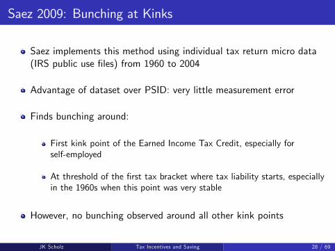
Saez 2009: Bunching at Kinks
Saez implements this method using individual tax return micro data(IRS public use files) from 1960 to 2004
Advantage of dataset over PSID: very little measurement error
Finds bunching around:
First kink point of the Earned Income Tax Credit, especially forself-employed
At threshold of the first tax bracket where tax liability starts, especiallyin the 1960s when this point was very stable
However, no bunching observed around all other kink points
JK Scholz ()Tax Incentives and Saving 28 / 69
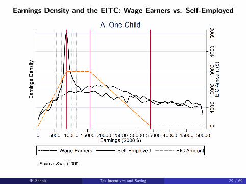
Earnings Density and the EITC: Wage Earners vs. Self-Employed
JK Scholz ()Tax Incentives and Saving 29 / 69

Earnings Density and the EITC: Wage Earners vs. Self-Employed
JK Scholz ()Tax Incentives and Saving 30 / 69

Taxable Income Density, 1960-1969: Bunching around First Kink
JK Scholz ()Tax Incentives and Saving 31 / 69

Taxable Income Density, 1960-1969: Bunching around First Kink
JK Scholz ()Tax Incentives and Saving 32 / 69

Why not more bunching at the kinks?
1 True elasticity response may be small2 Randomness in income generating process3 Information and salience
Liebman and Zeckhauser: "Schmeduling"Chetty and Saez (2009): information significantly affects bunching inan EITC field experiment
4 Adjustment costs and institutional constraints (Chetty et al., 2009)
JK Scholz ()Tax Incentives and Saving 33 / 69

Bianchi, Gudmundsson, and Zoega 2001
Use 1987 “no tax year” in Iceland as a natural experiment
In 1987-88, Iceland switched to a withholding-based tax system
Workers paid taxes on 1986 income in 1987; paid taxes on 1988income in 1988; 1987 earnings never taxed
Data: individual tax returns matched with data on weeks worked frominsurance database
Random sample of 9,274 individuals who filed income tax-returns in1986-88
JK Scholz ()Tax Incentives and Saving 34 / 69

General Observations
Per capita weeks worked in 1987 increased by 4.2% for women and2.4% for men.
There’s likely to be substantial heterogeneity.
People with children may have less flexibility than others.Secondary workers may already have substantial non-wage income fromtheir partners.
Tax rates range from 14.5% to 56.3% (average rates were 32% inother Nordic countries).
A major complication —all heck is breaking out during this period.
Unemployment, 0.7%! Inflation, 20% to 30%!Growth: 1985, 3.3%; 1986, 6%; 1987, 8.5% —real per capitadisposable income increased 25%The then slowed the economy, so GDP was stagnant into the 1990s.
JK Scholz ()Tax Incentives and Saving 35 / 69

JK Scholz ()Tax Incentives and Saving 36 / 69

JK Scholz ()Tax Incentives and Saving 37 / 69

JK Scholz ()Tax Incentives and Saving 38 / 69

JK Scholz ()Tax Incentives and Saving 39 / 69

Bianchi, Gudmundsson, and Zoega 2001
Large, salient change: ∆ log(1−MTR) ≈ 43%, much bigger thanmost studies
Note that elasticities reported in paper are w.r.t. average tax rates:
εL,T /E =∑(L87 − LA)/LA
∑T86/E86
εE ,T /E =∑(E87 − EA)/EA
∑T86/E86
Estimates imply hours elasticity w.r.t. marginal tax rate of roughly0.29
Not exactly clear how to interpret this elasticity (compensated static(Hicksian), intertemporal (Frisch).
JK Scholz ()Tax Incentives and Saving 40 / 69

Summary of Static Labor Supply Literature
1 Small elasticities for prime-age males
Probably institutional restrictions, need for one income, etc. prevent ashort-run response
2 Larger responses for workers who are less attached to labor force
Married women, low incomes, retirees
3 Responses driven by extensive margin
Extensive margin (participation) elasticity around 0.2
Intensive margin (hours) elasticity close 0
4 There is a rich literature on estimating models of intertemporal laborsupply, but we are instead turning to other issues.
JK Scholz ()Tax Incentives and Saving 41 / 69

Econometric Problem 4: Non-Hours Responses
Traditional literature focused purely on hours of work and labor forceparticipation
Problem: income taxes distort many margins beyond hours of work
More important responses may be on those margins
Hours very hard to measure (most ppl report 40 hours per week)
Two solutions in modern literature:
Focus on taxable income (wl) as a broader measure of labor supply(Feldstein 1995)
Focus on subgroups of workers for whom hours are better measured,e.g. taxi drivers. I won’t spend any time talking about taxi drivers.
JK Scholz ()Tax Incentives and Saving 42 / 69

Taxable Income Elasticities
Modern public finance literature focuses on taxable income elasticitiesinstead of hours/participation elasticities
Two main reasons
1 Convenient suffi cient statistic for all distortions created by income taxsystem (Feldstein 1999)
2 Data availability: taxable income is precisely measured in tax returndata
JK Scholz ()Tax Incentives and Saving 43 / 69

US Income Taxation: Trends
The biggest changes in MTRs are at the top
1 [Kennedy tax cuts]: 91% to 70% in ’63-65
2 [Reagan I, ERTA 81]: 70% to 50% in ’81-82
3 [Reagan II, TRA 86]: 50% to 28% in ’86-88
4 [Bush I tax increase]: 28% to 31% in ’91
5 [Clinton tax increase]: 31% to 39.6% in ’93
6 [Bush Tax cuts]: 39.6% to 35% in ’01-03
JK Scholz ()Tax Incentives and Saving 44 / 69

Saez 2004: Long-Run Evidence
Compares top 1% relative to the bottom 99%
Bottom 99% real income increases up to early 1970s and stagnatessince then
Top 1% increases slowly up to the early 1980s and then increasesdramatically up to year 2000.
Corresponds to the decrease in MTRs
Pattern exemplifies general theme of this literature: large responsesfor top earners, no response for rest of the population
JK Scholz ()Tax Incentives and Saving 45 / 69

$0
$5,000
$10,000
$15,000
$20,000
$25,000
$30,000
$35,000
$40,000
5%Marginal Tax Rate Average Income5%Marginal Tax Rate Average Income5%Marginal Tax Rate Average Income
0%
10%
15%
20%
25%
30%
35%
40%
5%
Bottom 99% Tax Units
Source: Saez 2004
Mar
gina
l Tax
Rat
e
1960
1962
1964
1966
1968
1970
1972
1974
1976
1978
1980
1982
1984
1986
1988
1990
1992
1994
1996
1998
2000
JK Scholz ()Tax Incentives and Saving 46 / 69

Top 1% Tax Units
20%
30%
40%
50%
60%
70%
80%
1960
1962
1964
1966
1968
1970
1972
1974
1976
1978
1980
1982
1984
1986
1988
1990
1992
1994
1996
1998
2000
Mar
gina
l Tax
Rat
e
$0
$100,000
$200,000
$300,000
$400,000
$500,000
$600,000
$700,000
$800,000
5%Marginal Tax Rate Average Income5%Marginal Tax Rate Average Income5%Marginal Tax Rate Average Income10%
Source: Saez 2004
0%
JK Scholz ()Tax Incentives and Saving 47 / 69

Saez-Veall 2005
Document changes in inequality.
Tax reporting or real?
Mobility: different or same people?
Married women and assortative mating?
What’s driving the trends?
Canada (individual tax base so can aggregate to the family, panel,and comparative study).
JK Scholz ()Tax Incentives and Saving 48 / 69

JK Scholz ()Tax Incentives and Saving 49 / 69

JK Scholz ()Tax Incentives and Saving 50 / 69

JK Scholz ()Tax Incentives and Saving 51 / 69

JK Scholz ()Tax Incentives and Saving 52 / 69

JK Scholz ()Tax Incentives and Saving 53 / 69

JK Scholz ()Tax Incentives and Saving 54 / 69

JK Scholz ()Tax Incentives and Saving 55 / 69

Feldstein 1995
First study of taxable income: Lindsey (1987) using cross-sectionsaround 1981 reform
Limited data and serious econometric problems
Feldstein (1995) estimates the effect of TRA86 on taxable income fortop earners
Constructs three income groups based on income in 1985
Looks at how incomes and MTR evolve from 1985 to 1988 forindividuals in each group using panel
JK Scholz ()Tax Incentives and Saving 56 / 69

JK Scholz ()Tax Incentives and Saving 57 / 69

Feldstein: Results
Feldstein obtains very high elasticities (above 1) for top earners
Implication: we were on the wrong side of the Laffer curve for the rich
Cutting tax rates would raise revenue
JK Scholz ()Tax Incentives and Saving 58 / 69

Feldstein: Econometric Criticisms
DD can give very biased results when elasticity differ by groups
Suppose that the middle class has a zero elasticity so that
∆ log(zM ) = 0
Suppose high income individuals have an elasticity of e so that
∆ log(zH ) = e∆ log(1− τH )
Suppose tax change for high is twice as large:
∆ log(1− τM ) = 10% and ∆ log(1− τH ) = 20%
Estimated elasticity e = e ·20%−020%−10% = 2e
JK Scholz ()Tax Incentives and Saving 59 / 69

Feldstein: Econometric Criticisms
Sample size: results driven by very few observations (Slemrod 1996).
Slemrod’s "hierarchy" of responses: timing, financial, and real. Realchanges are hardest to execute.
Auten-Carroll (1999) replicate results on larger Treasury dataset
Find a smaller elasticity: 0.65
Different trends across income groups (Goolsbee 1998)
Triple difference that nets out differential prior trends yields elasticity<0.4 for top earners
JK Scholz ()Tax Incentives and Saving 60 / 69

Slemrod: Shifting vs. “Real”Responses
Slemrod (1996) studies “anatomy”of the behavioral responseunderlying change in taxable income
Shows that large part of increase is driven by shift between C corpincome to S corp income
Looks like a supply side story but government is actually losing revenueat the corporate tax level
Shifting across tax bases not taken into account in Feldstein effi ciencycost calculations
JK Scholz ()Tax Incentives and Saving 61 / 69

FIGURE 7
The Top 1% Income Share and Composition, 19602000
Source: Saez 2004
0%
2%
4%
6%
8%
10%
12%
14%
16%
18%
1960
1962
1964
1966
1968
1970
1972
1974
1976
1978
1980
1982
1984
1986
1988
1990
1992
1994
1996
1998
2000
Wages SCorp. Partner. Sole P. Dividends Interest Other
JK Scholz ()Tax Incentives and Saving 62 / 69

Goolsbee: Intertemporal Shifting
Goolsbee (2000) hypothesizes that top earners’ability to re-timeincome drives much of observed responses
Analogous to identification of Frisch elasticity instead of compensatedelasticity
Regression specification:
TLI = α+ β1 log(1− taxt ) + β2 log(1− taxt+1)
Long run effect is β1 + β2
Uses ExecuComp data to study effects of the 1993 Clinton taxincrease on executive pay
JK Scholz ()Tax Incentives and Saving 63 / 69

JK Scholz ()Tax Incentives and Saving 64 / 69

Goolsbee 2000
Most affected groups (income>$250K) had a surge in income in 1992(when reform was announced) relative to 1991 followed by a sharpdrop in 1993
Simple DD estimate would find a large effect here, but it would bepicking up pure re-timing
Concludes that long run effect is 20x smaller than substitution effect
Effects driven almost entirely by retiming exercise of options
Long run elasticity <0.4 and likely close to 0
JK Scholz ()Tax Incentives and Saving 65 / 69

Gruber and Saez 2002
First study to examine taxable income responses for generalpopulation, not just top earners
Use data from 1979-1991 on all tax changes available rather than asingle reform
Simulated instruments methodology
Step 1: Simulate tax rates based on period t income and characteristics
MTRPt+3 = ft+3(yt ,Xt )
MTRt+3 = ft+3(yt+3,Xt+3)
Step 2 [first stage]: Regress log(1−MTRt+3)− log(1−MTRt ) onlog(1−MTRPt+3)− log(1−MTRt )
Step 3 [second stage]: Regress ∆ logTI on predicted value from firststage
Isolates changes in laws (ft) as the only source of variation in tax ratesJK Scholz ()Tax Incentives and Saving 66 / 69

JK Scholz ()Tax Incentives and Saving 67 / 69

Gruber and Saez: Results
Find an elasticity of roughly 0.3-0.4 with splines
But this is very fragile (Giertz 2008)
Sensitive to exclusion of low incomes (min income threshold)
Sensitive to controls for mean reversion
Subsequent studies find smaller elasticities using data from othercountries
JK Scholz ()Tax Incentives and Saving 68 / 69

Taxable Income Literature: Summary
Large responses for the rich, mostly intertemporal substitution andshifting
Responses among lower incomes small at least in short run
Perhaps not surprising if they have little flexibility to change earnings
Pattern confirmed in many settings (e.g. Kopczuk 2009 - Polish flattax reform)
But many methodological problems remain to be resolved
Econometric issues: mean reversion, appropriate counterfactuals
Which elasticity is being identified?
JK Scholz ()Tax Incentives and Saving 69 / 69