Public Corruption for Gain in America: The Costly

UNLV Theses, Dissertations, Professional Papers, and Capstones

5-1-2012

Public Corruption for Gain in America: The Costly Consequences Public Corruption for Gain in America: The Costly Consequences

of Violating Public Trust of Violating Public Trust

Yvonne Atkinson Gates University of Nevada, Las Vegas

Follow this and additional works at: https://digitalscholarship.unlv.edu/thesesdissertations

Part of the American Politics Commons, and the Public Administration Commons

Repository Citation Repository Citation Gates, Yvonne Atkinson, "Public Corruption for Gain in America: The Costly Consequences of Violating Public Trust" (2012). UNLV Theses, Dissertations, Professional Papers, and Capstones. 1565. http://dx.doi.org/10.34917/4332546

This Dissertation is protected by copyright and/or related rights. It has been brought to you by Digital Scholarship@UNLV with permission from the rights-holder(s). You are free to use this Dissertation in any way that is permitted by the copyright and related rights legislation that applies to your use. For other uses you need to obtain permission from the rights-holder(s) directly, unless additional rights are indicated by a Creative Commons license in the record and/or on the work itself. This Dissertation has been accepted for inclusion in UNLV Theses, Dissertations, Professional Papers, and Capstones by an authorized administrator of Digital Scholarship@UNLV. For more information, please contact [email protected].

http://library.unlv.edu/

http://library.unlv.edu/

https://digitalscholarship.unlv.edu/thesesdissertations

https://digitalscholarship.unlv.edu/thesesdissertations?utm_source=digitalscholarship.unlv.edu%2Fthesesdissertations%2F1565&utm_medium=PDF&utm_campaign=PDFCoverPages

http://network.bepress.com/hgg/discipline/387?utm_source=digitalscholarship.unlv.edu%2Fthesesdissertations%2F1565&utm_medium=PDF&utm_campaign=PDFCoverPages

http://network.bepress.com/hgg/discipline/398?utm_source=digitalscholarship.unlv.edu%2Fthesesdissertations%2F1565&utm_medium=PDF&utm_campaign=PDFCoverPages

http://dx.doi.org/10.34917/4332546

mailto:[email protected]

PUBLIC CORRUPTION FOR GAIN IN AMERICA:

THE COSTLY CONSEQUENCES OF

VIOLATING PUBLIC TRUST

by

Yvonne Atkinson Gates

Bachelor of Science, Political Science University of Nevada, Las Vegas

1978

Master of Public Administration University of Nevada, Las Vegas

1982

A dissertation submitted in partial fulfillment of the requirements for the

Doctor of Philosophy Degree in Public Affairs

Department of Public Administration Greenspun College of Urban Affairs

Graduate College

University of Nevada, Las Vegas May 2012

© 2012 by Yvonne Atkinson Gates

All Rights Reserved

ii

THE GRADUATE COLLEGE

We recommend the dissertation prepared under our supervision by


Entitled

Public Corruption for Gain in America: The Costly Consequences of Violating Public Trust be accepted in partial fulfillment of the requirements for the degree of

Doctor of Philosophy in Public Affairs School of Environmental and Public Affairs

Lee Bernick, Ph.D., Committee Chair

David Damore, Ph.D., Committee Member

Christopher Stream, Ph.D., Committee Member

Dina Titus, Ph.D., Graduate College Representative

Ronald Smith, Ph. D., Vice President for Research and Graduate Studies and Dean of the Graduate College

May 2012

iii

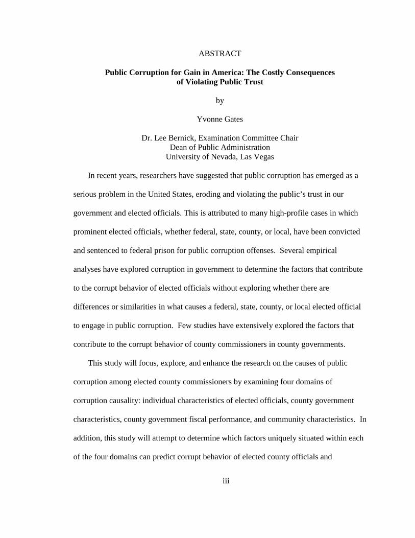
ABSTRACT

Public Corruption for Gain in America: The Costly Consequences of Violating Public Trust

by

Yvonne Gates

Dr. Lee Bernick, Examination Committee Chair Dean of Public Administration

University of Nevada, Las Vegas

In recent years, researchers have suggested that public corruption has emerged as a

serious problem in the United States, eroding and violating the public’s trust in our

government and elected officials. This is attributed to many high-profile cases in which

prominent elected officials, whether federal, state, county, or local, have been convicted

and sentenced to federal prison for public corruption offenses. Several empirical

analyses have explored corruption in government to determine the factors that contribute

to the corrupt behavior of elected officials without exploring whether there are

differences or similarities in what causes a federal, state, county, or local elected official

to engage in public corruption. Few studies have extensively explored the factors that

contribute to the corrupt behavior of county commissioners in county governments.

This study will focus, explore, and enhance the research on the causes of public

corruption among elected county commissioners by examining four domains of

corruption causality: individual characteristics of elected officials, county government

characteristics, county government fiscal performance, and community characteristics. In

addition, this study will attempt to determine which factors uniquely situated within each

of the four domains can predict corrupt behavior of elected county officials and

iv

convictions for public corruption. Lastly, this study will attempt to determine if General

Strain Theory can provide a theoretical framework for understanding the causes of public

corruption and, if so, to what degree it can predict whether elected county officials will

engage in corrupt behavior.

The quantitative study sample for this research consists of data collected on large

urban counties in which county officials were convicted or indicted of public corruption

between the fiscal years of 2000 and 2009. Additional study samples consist of data

collected on more than 100 large urban counties with no cases of public corruption. Both

categories of data were derived from counties with populations of 300,000 or more in

which there were indictments, convictions, and no indictments or convictions of county

officials for the 2000 2009 fiscal years. The unit of analysis consists of county

commissioners from large urban counties convicted and not convicted of public

corruption. To determine which factors contribute to the specific research questions and

related hypotheses, the study will explore 26 explanatory variables within four domains

contained in the research General Models. It will use logistic regression procedures and

analytical prediction of probability tools to discover relationships between the dependent

and the independent variables.

This study attempts to determine the causes of public corruption by examining and

answering four specific research questions:

1. Are there specific personal characteristics that encourage or discourage county

officials to engage in public corruption?

2. What are the governmental characteristics that contribute to public corruption?

3. What role does government fiscal stability play in explaining public corruption?

v

4. Do communities with high civic involvement have less public corruption?

vi

ACKNOWLEDGMENTS

This project has benefited from the help of numerous people. First, I would like to

thank various individuals at the University of Nevada, Las Vegas, including my

dissertation committee and Dr. Thom Reilly, a former faculty member, who was always

responsive and offered important assistance and support. Dr. Lee Bernick and Dr. David

Damore provided guidance, wisdom, and encouragement that have been essential to my

academic pursuits and completion of this endeavor. Dr. Damore provided critical

assistance during my quantitative analysis process (reminding me often of my objective),

and Dr. Bernick, my committee chair, provided direction at key stages of the process and

was encouraging throughout. Dr. Dina Titus took the time to review my research in

detail and offered valuable suggestions. Dr. Christopher Stream offered guidance and

support in identifying additional corruption cases.

Special thanks are offered to many friends who provided encouragement and a

special friendship; their support was invaluable. Bobby, Melissa, Leon, Casey, Patricia,

and Winnifred were the best; their friendship is rare and greatly appreciated.

I thank my husband and children for being there, providing me with encouragement

and understanding throughout my pursuit. My achievements would not have been

possible without my family’s support.

Lastly, the support and reassurances of my sisters, particularly Isophine, were what I

needed to get through this journey; their support made it possible for me to achieve this

goal.

vii

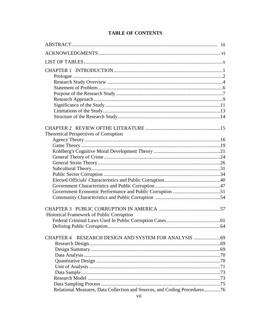
TABLE OF CONTENTS

ABSTRACT ..................................................................................................................... iii

ACKNOWLEDGMENTS ................................................................................................. vi

LIST OF TABLES ...............................................................................................................x

CHAPTER 1 INTRODUCTION .......................................................................................1 Prologue ........................................................................................................................2 Research Study Overview ............................................................................................4 Statement of Problem ....................................................................................................6 Purpose of the Research Study .....................................................................................7 Research Approach .......................................................................................................9 Significance of the Study ............................................................................................11 Limitations of the Study..............................................................................................13 Structure of the Research Study ..................................................................................14 CHAPTER 2 REVIEW OFTHE LITERATURE ............................................................15 Theoretical Perspectives of Corruption Agency Theory ............................................................................................................16 Game Theory ...............................................................................................................19 Kohlberg's Cognitive Moral Development Theory .....................................................21 General Theory of Crime .............................................................................................24 General Strain Theory ..................................................................................................26 Subcultural Theory.......................................................................................................31 Public Sector Corruption .............................................................................................34 Elected Officials' Characteristics and Public Corruption.............................................40 Government Characteristics and Public Corruption ....................................................47 Government Economic Performance and Public Corruption ......................................51 Community Characteristics and Public Corruption ....................................................54 CHAPTER 3 PUBLIC CORRUPTION IN AMERICA .................................................57 Historical Framework of Public Corruption Federal Criminal Laws Used In Public Corruption Cases ...........................................61 Defining Public Corruption..........................................................................................64 CHAPTER 4 RESEARCH DESIGN AND SYSTEM FOR ANALYSIS .....................69 Research Design.........................................................................................................69 Design Summary ........................................................................................................69 Data Analysis .............................................................................................................70 Quantitative Design ...................................................................................................70 Unit of Analysis .........................................................................................................71 Data Sample ...............................................................................................................73 Research Model ..........................................................................................................73 Data Sampling Process ...............................................................................................75 Relational Measures, Data Collection and Sources, and Coding Procedures .............76

viii

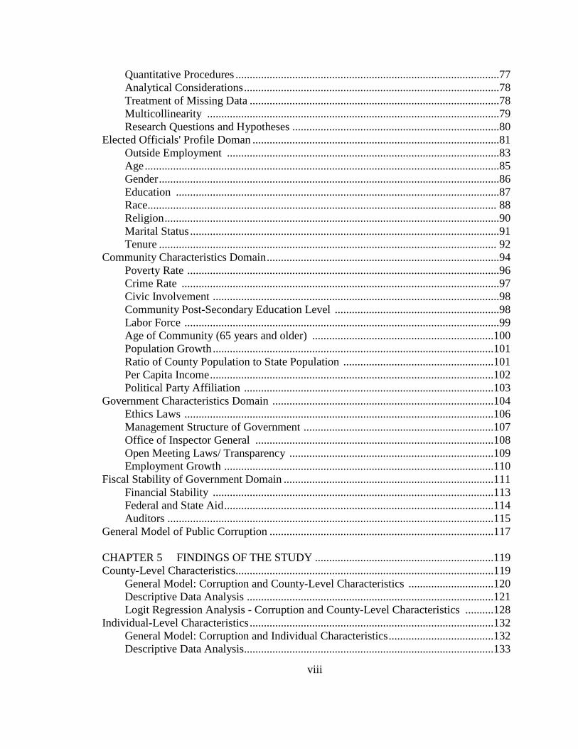
Quantitative Procedures .............................................................................................77 Analytical Considerations ..........................................................................................78 Treatment of Missing Data ........................................................................................78 Multicollinearity .......................................................................................................79 Research Questions and Hypotheses .........................................................................80 Elected Officials' Profile Doman .......................................................................................81 Outside Employment ................................................................................................83 Age .............................................................................................................................85 Gender ........................................................................................................................86 Education ..................................................................................................................87 Race........................................................................................................................... 88 Religion ......................................................................................................................90 Marital Status .............................................................................................................91 Tenure ....................................................................................................................... 92 Community Characteristics Domain ..................................................................................94 Poverty Rate ..............................................................................................................96 Crime Rate ................................................................................................................97 Civic Involvement .....................................................................................................98 Community Post-Secondary Education Level ..........................................................98 Labor Force ...............................................................................................................99 Age of Community (65 years and older) ................................................................100 Population Growth ...................................................................................................101 Ratio of County Population to State Population .....................................................101 Per Capita Income ....................................................................................................102 Political Party Affiliation ........................................................................................103 Government Characteristics Domain ..............................................................................104 Ethics Laws .............................................................................................................106 Management Structure of Government ...................................................................107 Office of Inspector General ....................................................................................108 Open Meeting Laws/ Transparency ........................................................................109 Employment Growth ...............................................................................................110 Fiscal Stability of Government Domain ..........................................................................111 Financial Stability ...................................................................................................113 Federal and State Aid ...............................................................................................114 Auditors ...................................................................................................................115 General Model of Public Corruption ...............................................................................117 CHAPTER 5 FINDINGS OF THE STUDY ...............................................................119 County-Level Characteristics...........................................................................................119 General Model: Corruption and County-Level Characteristics ..............................120 Descriptive Data Analysis .......................................................................................121 Logit Regression Analysis - Corruption and County-Level Characteristics ..........128 Individual-Level Characteristics ......................................................................................132 General Model: Corruption and Individual Characteristics .....................................132 Descriptive Data Analysis........................................................................................133

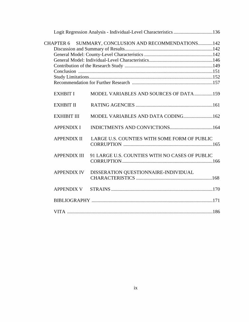
ix

Logit Regression Analysis - Individual-Level Characteristics ................................136 CHAPTER 6 SUMMARY, CONCLUSION AND RECOMMENDATIONS............142 Discussion and Summary of Results........................................................................142 General Model: County-Level Characteristics ........................................................142 General Model: Individual-Level Characteristics ....................................................146 Contribution of the Research Study ........................................................................149 Conclusion ..............................................................................................................151 Study Limitations .....................................................................................................152 Recommendation for Further Research ..................................................................157 EXHBIT I MODEL VARIABLES AND SOURCES OF DATA ...............159 EXHBIT II RATING AGENCIES ...............................................................161 EXHIBIT III MODEL VARIABLES AND DATA CODING........................162 APPENDIX I INDICTMENTS AND CONVICTIONS...................................164 APPENDIX II LARGE U.S. COUNTIES WITH SOME FORM OF PUBLIC CORRUPTION .........................................................................165 APPENDIX III 91 LARGE U.S. COUNTIES WITH NO CASES OF PUBLIC CORRUPTION ..........................................................................166 APPENDIX IV DISSERATION QUESTIONNAIRE-INDIVIDUAL CHARACTERISTICS ..............................................................168 APPENDIX V STRAINS ...................................................................................170 BIBLIOGRAPHY ...................................................................................................171 VITA .......................................................................................................................186

x

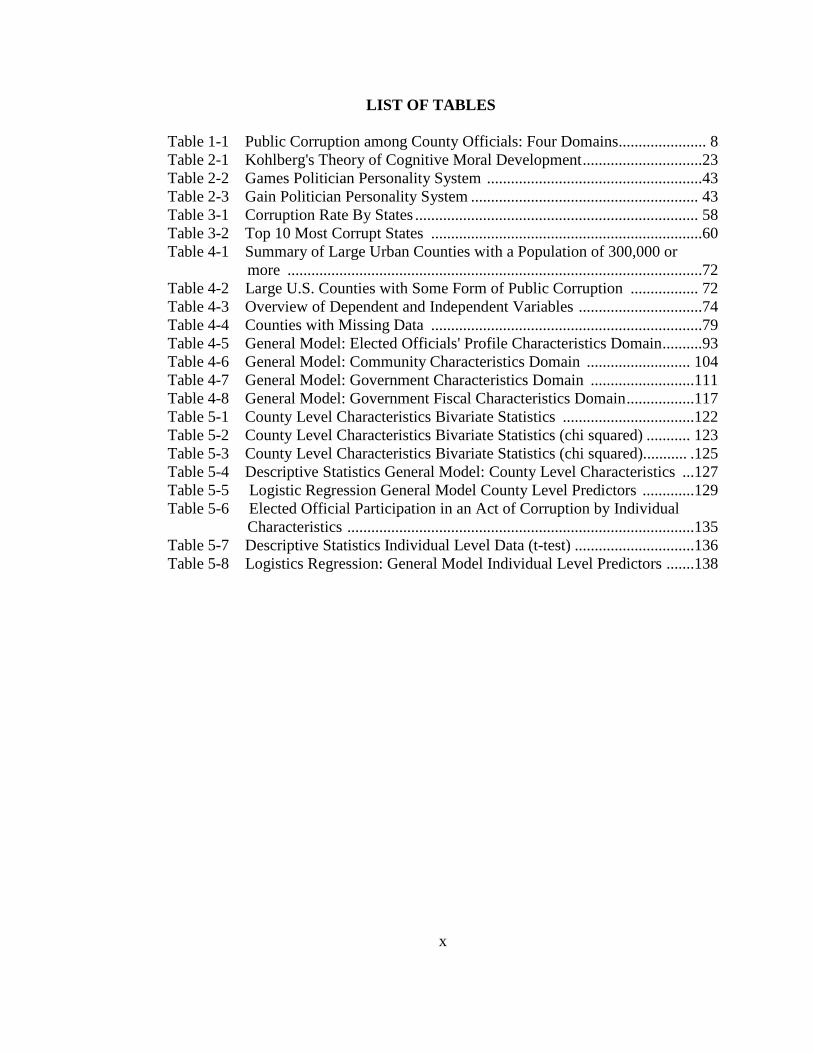
LIST OF TABLES

Table 1-1 Public Corruption among County Officials: Four Domains...................... 8 Table 2-1 Kohlberg's Theory of Cognitive Moral Development ..............................23 Table 2-2 Games Politician Personality System ......................................................43 Table 2-3 Gain Politician Personality System ......................................................... 43 Table 3-1 Corruption Rate By States ....................................................................... 58 Table 3-2 Top 10 Most Corrupt States ....................................................................60 Table 4-1 Summary of Large Urban Counties with a Population of 300,000 or more ........................................................................................................72 Table 4-2 Large U.S. Counties with Some Form of Public Corruption ................. 72 Table 4-3 Overview of Dependent and Independent Variables ...............................74 Table 4-4 Counties with Missing Data ....................................................................79 Table 4-5 General Model: Elected Officials' Profile Characteristics Domain ..........93 Table 4-6 General Model: Community Characteristics Domain .......................... 104 Table 4-7 General Model: Government Characteristics Domain ..........................111 Table 4-8 General Model: Government Fiscal Characteristics Domain .................117 Table 5-1 County Level Characteristics Bivariate Statistics .................................122 Table 5-2 County Level Characteristics Bivariate Statistics (chi squared) ........... 123 Table 5-3 County Level Characteristics Bivariate Statistics (chi squared)........... .125 Table 5-4 Descriptive Statistics General Model: County Level Characteristics ...127 Table 5-5 Logistic Regression General Model County Level Predictors .............129 Table 5-6 Elected Official Participation in an Act of Corruption by Individual Characteristics .......................................................................................135 Table 5-7 Descriptive Statistics Individual Level Data (t-test) ..............................136 Table 5-8 Logistics Regression: General Model Individual Level Predictors .......138

1

CHAPTER 1

INTRODUCTION

Mary Buckelew was once called the most powerful woman in Jefferson County,

Alabama. She was the first woman ever elected to the county commission, in November

1990, and served in the position until 2006. She even served as president of the Board of

County Commission from 1990–1998. Commissioner Buckelew was a savvy political

operative who developed a reputation for having an uncanny ability to find consensus

among a bitterly divided board. To highlight her accomplishments, in 1997 Governing

Magazine honored her as one of its “Public Officials of the Year.” But Mary Buckelew’s

power and popularity evaporated when she was forced out of office for public corruption.

Commissioner Buckelew’s downfall began in 1996 when the Jefferson County

Commission entered into a court-ordered consent decree that mandated the renovation of

the county’s sewer system. To fund the renovation, the County Commission decided to

participate in several bond offerings and numerous bond swap agreements. Between

March 2003 and December 2004, the commission approved five bond offerings and four

swap agreements worth billions of dollars.

Commissioner Buckelew and the Jefferson County finance committee participated in

the approval of all these transactions. During the process, Commissioner Buckelew, a

number of county administrative staff, and an investment banker hired by Jefferson

County to oversee the bond transactions traveled to New York City on several occasions

to discuss them with other investment firms and officials. During one trip to New York,

Commissioner Buckelew visited a Salvatore Ferragamo store on Fifth Avenue and saw a

pair of shoes and a purse she admired on sale for about $1,500. On another trip,

2

Commissioner Buckelew admired other items at the same store costing a total of $1,119.

It was later discovered that the investment banker hired by the county had purchased

these items for Commissioner Buckelew on both occasions and mailed them to her office

at the Jefferson County government building. During a third trip to New York in 2004,

this banker paid approximately $1,400 for Commissioner Buckelew to spend the day at a

New York City spa. In total, Commissioner Buckelew received nearly $5,000 in gifts

from the investment banker hired by the Jefferson County Commission to oversee and

manage the bonds allocated to renovate the county’s sewer system. The investment

banker and his firm received approximately $7.1 million in brokerage fees.

Mary Buckelew would later plead guilty to a charge of obstruction of justice and

agree to cooperate with the investigators probing public corruption in Jefferson County.

As part of her plea agreement, Buckelew faced imprisonment for up to 20 years, a fine of

up to $250,000, or both; supervised release of not more than three years; and a special

assessment fee of $100 per count. Buckelew was later sentenced to three years’

probation, 200 hours of community service, and a $20,000 fine for lying to a federal

grand jury during its probe of the county. In recent months, Jefferson County has

defaulted on its bond payments and is considering filing for bankruptcy.

Prologue

The corruption of public officials like Mary Buckelew, and public corruption in

general, are not new problems. Public corruption has existed for at least 4,000 to 5,000

years, if not longer, according to Bardhan (1997).1

1The fact that corruption is not a modern phenomenon is also emphasized by Vito Tanzi (1998), who stated, “Corruption is not a

new phenomenon” (p. 559). Two thousand years ago, Kautilya, the prime minister of an Indian kingdom, had already written a book, Arthasastra, discussing it. Seven centuries ago, Dante placed bribers in the deepest part of Hell, reflecting the medieval distaste for corrupt behavior. Shakespeare gave corruption a prominent role in some of his plays, and the U.S. Constitution explicitly names bribery and treason as two crimes that can justify the impeachment of a president.

Explanations of the reasons behind

3

public corruption have been offered for nearly as long. However, the “study of

corruption by academics, policy-makers or self-styled analysts is a more recent

phenomenon” (Mukherjee 2004, p. 1).2

As early as the 1960s, political scientists, economists, and sociologists focused their

attention on political corruption in terms of its impact on government policy and the

economy. Benson (1978) notes that “Alexis de Tocqueville, in his classic book,

Democracy in America, identifies corruption as a danger of and to democracy, as well as

a potential component of it” (p. 1).

This research study will review and identify the impact public corruption has on our

governmental systems, citizens, and the legitimacy of democracy itself. The presence of

corruption in the United States, if unchecked, could undermine the purpose of

government and the rights and the needs of the governed, and create widespread

economic problems for both government and the governed. Indeed, according to Warren

(2004), “Corruption creates inefficiencies in deliveries of public services, not only in the

form of a tax on public expenditures, but by shifting public activities towards those

sectors in which it is possible for those engaged in corrupt exchanges to benefit.” He

goes on to point out that “corruption also undermines the culture of democracy [by]

eroding trust” (p. 328). Clearly, corruption in the present-day U.S. can compromise the

purpose of government and ruin the economic, political, and social stability of its people.

Consequently, it is important to explore those factors that account for public corruption in

county government.

2

One of the earliest academic works on corruption is The Moral Basis of a Backward Society (Banfield 1958). Other prominent works written after World War II include “Economic Development Through Bureaucratic Corruption” (Leff 1964); Political Corruption: A Handbook (Heidenheimer et al. 1989); Comparative Political Corruption (Scott 1972); Political Order in Changing Societies (Huntington 1968); and Corruption in Developing Countries (Wraith and Simkins 1963).

4

An analysis of public corruption in county government is vital because counties are

major institutions in our political system. County governments serve as agents of the

state, with monies flowing from state government to counties to implement programs and

services that citizens need. In many cases, large urban counties have greater authority,

provide a greater degree of service, and have a greater span of power and influence than

cities do. The power, authority, and influence that county government has, as well as its

overall responsibilities in the delivery of services, justify the need to study public

corruption in county government.

Research has shown the negative impact public corruption can have on government

(Warren 2004), but that is not the focal point of this research. Rather, this study seeks to

understand why public corruption exists in our system of county governments. It will

review literature, develop models, and study the cases of various county officials in an

attempt to understand the elements and factors that contribute to the corruption of public

officials in county government.

In a close review of the literature, several theoretical perspectives emerged about

corruption among county officials. The rest of this section will discuss the limitations

and important components necessary to explaining corruption among county officials and

reveal a platform for selecting the best-suited theory for this research study: General

Strain Theory (GST).

Research Study Overview

The presence of public corruption in government suggests that corruption has a

broad effect on people: it creates a system of mistrust among citizens, thereby

diminishing the importance of government and influencing the rule of law and regulation,

5

which in turn inflicts enormous economic, political, and social costs on society. This

research study is a comprehensive review designed to examine, explore, and explain

public corruption among officials in county government utilizing GST. Agnew (1992)

described GST as an individual’s “actual or anticipated failure to achieve positively

valued goals, actual or anticipated removal of positively valued stimuli, and actual or

anticipated presentation of negative stimuli,” all of which can result in strain (p. 59).

Strain emerges from negative relationships with others, leading individuals to engage in

criminal behavior. This research study will evaluate how GST manifests itself in the day-

to-day activities of county officials in their efforts to carry out their duties as

representatives of the public.

To further understand how the theoretical perspective of GST could explain a county

official’s decision to engage in public corruption, explanatory variables were developed

with the intent of examining the relationship between public corruption and the personal

characteristics of elected officials. The General Model will also explore the relationship

between public corruption and county-level characteristics as they may apply to large

urban counties with cases of public corruption, as well as those counties with no cases of

public corruption.

The application of GST is appealing in this instance because of the limited research

conducted to understand the effect the theory has on corruption in county government.

Although recent progress has advanced our understanding of public corruption and

explored how it affects government, there is little information (and few empirical studies)

describing specific variables that explain elected county officials’ decisions to engage in

6

corrupt behavior. In fact, GST has limited exposure in the area of public corruption

hypothesis testing, which creates an opportunity worthy of review.

This research study builds on the premise that GST might explain the factors that

contribute to white-collar crime, including public corruption committed by elected county

officials.

Statement of Problem

Some county officials choose to engage in public corruption in today’s political

environment, while others do not. In the context of this study, the following questions

merit answers:

1. What factors explain public corruption in today’s county government?

2. Will answering the question of public corruption provide insight into what

may deter, reduce, or minimize corruption in county government?

Amundsen (1999) stated, “Corruption is one of the greatest challenges of the

contemporary world. It undermines good government, fundamentally distorts public

policy, leads to the misallocation of resources, harms the public sector and private sector

development, and particularly hurts the poor” (p. 1). The presence of corruption in

county government and its effects on today’s society create enormous pressures for an

honest government. Benson (1978) opined: “The loss of citizens’ confidence in a

government which citizens know is cheating has a profound effect on the democratic

process” (p. 51). Benson also postulated, “Corruption can cost a government, and its

taxpayers, large sums through both ‘honest’ graft, and the overburdening of the

government exchequer” (p. 208). Clearly, the presence of public corruption has a broad

effect on people and does little to eliminate their mistrust of government and the public

7

officials who engage in corruption. In fact, Musgrave (1959) suggested public corruption

weakens the purpose and possibility of an effective government by undermining the

functions of macroeconomic stabilization, income redistribution, and resource allocation,

which are the three primary functions of public institutions today. Moreover, without a

thorough knowledge of the causes of public corruption, the American public’s distrust of

public officials and their ability to deliver key public services will continue to grow.

The literature review explored the importance of implementing stringent

anticorruption policies and ethics laws to determine their effectiveness in reducing public

corruption. Although little is known about the elements that contribute to public

corruption in the contemporary U.S., analyzing it with GST will add to the body of

knowledge in this area of inquiry. Additionally, exploring the relationship of GST to

local government and elected officials, and examining its effect on public corruption, are

both new ideas that should generate further interest.

Purpose of the Research Study

This research study has three objectives.

First, it will attempt to use GST to explain public corruption in local government by

county officials convicted in federal court. It will study whether GST is a plausible

model to explain corruption within the four domains of elected officials’ characteristics,

county government characteristics, governmental fiscal stability, and community

stability.

Second, this study will examine the decisions of two groups of county officials who

take divergent roads in their political careers to explain public corruption and predict

what factors could be used to stop officials from engaging in it.

8

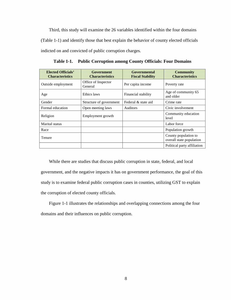
Third, this study will examine the 26 variables identified within the four domains

(Table 1-1) and identify those that best explain the behavior of county elected officials

indicted on and convicted of public corruption charges.

Table 1-1. Public Corruption among County Officials: Four Domains

Elected Officials’ Characteristics

Government Characteristics

Governmental Fiscal Stability

Community Characteristics

Outside employment Office of Inspector General Per capita income Poverty rate

Age Ethics laws Financial stability Age of community 65 and older

Gender Structure of government Federal & state aid Crime rate Formal education Open meeting laws Auditors Civic involvement

Religion Employment growth Community education level

Marital status Labor force Race Population growth

Tenure County population to overall state population

Political party affiliation

While there are studies that discuss public corruption in state, federal, and local

government, and the negative impacts it has on government performance, the goal of this

study is to examine federal public corruption cases in counties, utilizing GST to explain

the corruption of elected county officials.

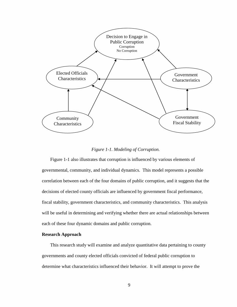
Figure 1-1 illustrates the relationships and overlapping connections among the four

domains and their influences on public corruption.

9

Figure 1-1. Modeling of Corruption.

Figure 1-1 also illustrates that corruption is influenced by various elements of

governmental, community, and individual dynamics. This model represents a possible

correlation between each of the four domains of public corruption, and it suggests that the

decisions of elected county officials are influenced by government fiscal performance,

fiscal stability, government characteristics, and community characteristics. This analysis

will be useful in determining and verifying whether there are actual relationships between

each of these four dynamic domains and public corruption.

Research Approach

This research study will examine and analyze quantitative data pertaining to county

governments and county elected officials convicted of federal public corruption to

determine what characteristics influenced their behavior. It will attempt to prove the

Elected Officials Characteristics


Government Fiscal Stability


Decision to Engage in Public Corruption

Corruption No Corruption

10

applicability of GST as the theory best suited to examining public corruption. The

research will focus on former elected county officials indicted and convicted of federal

public corruption charges and their counterparts from the same counties who were not

indicted or convicted, using data and information from fiscal years 2000 to 2009. This

study will analyze the fiscal policies, oversight, and community characteristics of county

governments that had cases of public corruption, but the primary purpose of this study is

to determine the impact GST has on governments, communities, and elected county

officials.

Much of the data analyzed was gathered from public information sources. The study

is unique in that the public officials who are its subjects were federally indicted or

convicted; therefore, much of the data was obtained through the Public Access to Court

Electronic Records system, a database of federally adjudicated court cases.

Agnew (1992) suggested that strain does not need to be specifically tied to economic

status because it is considered a psychological reaction to any perceived negative aspects

of one’s social environment, or as Agnew further stated, “negative relationships with

others... in which the individual is not treated as he or she wants to be treated” (p. 48).

In summary, this research study postulates that GST will explain the corruption

offenses of public officials based on each official’s profile characteristics, community

characteristics, and the influences of county government.

The data analysis for this study consisted of a two-step process to test the

hypotheses. First, the analysis examined data pertaining to county governments with

convicted officials and county governments with no convicted officials. Second, a

comparative study was conducted of elected county officials from those counties with

11

indicted and convicted public officials and those counties without officials indicted or

convicted of public corruption. The results of these analyses will be used in this paper to

identify the variables that explain why county officials do or do not elect to engage in

acts of public corruption.

Significance of the Study

Government is the cornerstone of a democracy; therefore, it has a responsibility to

maintain the highest level of integrity, free of political conflicts and public corruption.

The primary purpose of elected public officials is to serve and represent the interests of

the people who elected them, without regard to personal gain. If corruption invades our

system of government, how can citizens expect trustworthy and effective government?

As Benson (1978) stated, “Political corruption has become a serious liability to American

life” (p. 5). Whether it surfaces in federal, state, municipal, or county governments,

corruption deters the formation of honest and effective government.

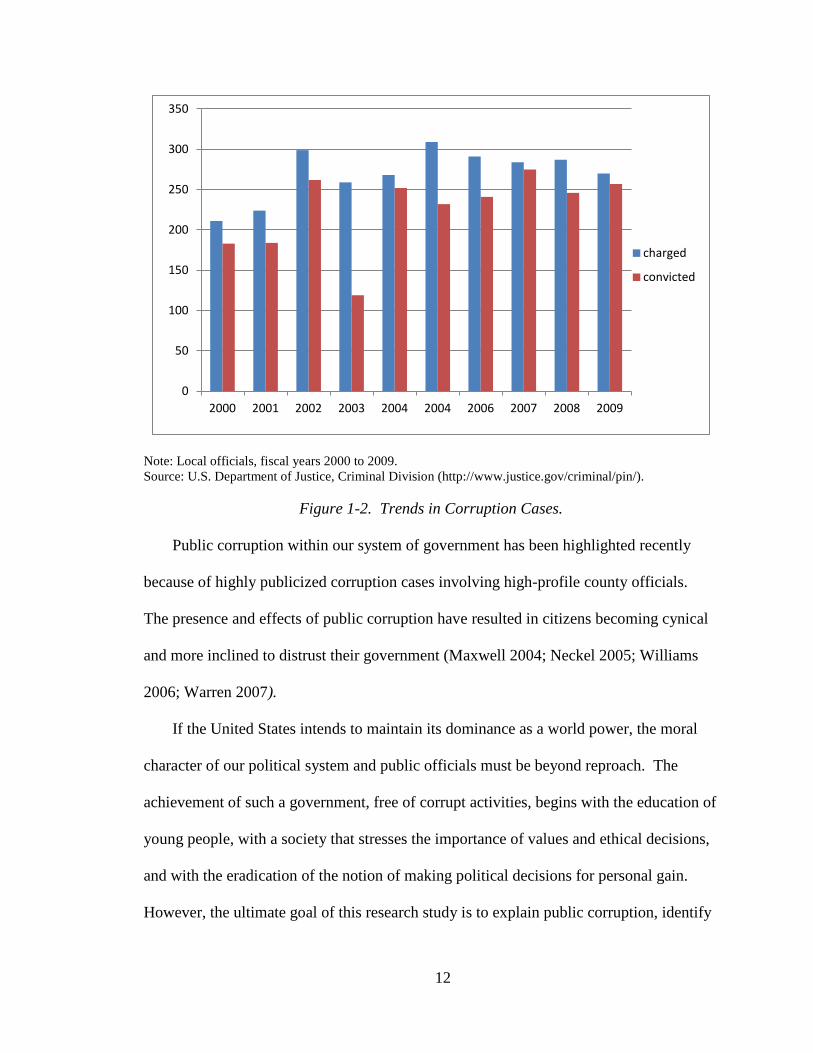
Data from the U.S. Department of Justice’s Public Integrity Section (2009) suggest

that there have been significant increases in corruption within all levels of government in

the past 20 years. Figure 1-2 displays the increases in corruption cases in local

government and in the number of local elected officials charged with corruption over the

past 10 years. The data show that local government convictions have increased by 71

percent and the number of local government officials charged with corruption has

increased by 78 percent over those same 10 years. It appears the federal government has

a successful record of prosecuting corruption cases and getting plea agreements from

defendants.

12

Note: Local officials, fiscal years 2000 to 2009. Source: U.S. Department of Justice, Criminal Division (http://www.justice.gov/criminal/pin/).

Figure 1-2. Trends in Corruption Cases.

Public corruption within our system of government has been highlighted recently

because of highly publicized corruption cases involving high-profile county officials.

The presence and effects of public corruption have resulted in citizens becoming cynical

and more inclined to distrust their government (Maxwell 2004; Neckel 2005; Williams

2006; Warren 2007).

If the United States intends to maintain its dominance as a world power, the moral

character of our political system and public officials must be beyond reproach. The

achievement of such a government, free of corrupt activities, begins with the education of

young people, with a society that stresses the importance of values and ethical decisions,

and with the eradication of the notion of making political decisions for personal gain.

However, the ultimate goal of this research study is to explain public corruption, identify

0

50

100

150

200

250

300

350

2000 2001 2002 2003 2004 2004 2006 2007 2008 2009

charged

convicted

13

the indicators of corruption, and use that information to offer suggestions to reduce

corruption, thereby restoring public trust in government and in our public officials.

Limitations of the Study

This research study was designed to study cases of public corruption in county

government; however, a review of the literature showed that the number of federal

conviction cases for county officials from 2000 to 2009 was smaller than anticipated.

Therefore, this study focused on the indictments of county elected officials, including

many that ultimately became convictions. Further research revealed a smaller number of

corruption cases than originally anticipated from large urban counties. All in all, case

reviews identified approximately 65 federal conviction cases; 12 were excluded from the

study, however, because they occurred in small counties with populations of less than

300,000 or took place before 2000. The expectation was that data prior to 2000 would be

difficult to obtain from small to mid-sized counties, which indeed turned out to be the

case; not only was it difficult to collect data prior to 2000, it was difficult to verify its

accuracy. Such limitations may have a negative impact on the validity of the study.

Because of the limited number of public corruption cases, the research pool was

expanded to include cases in which there were both indictments and convictions, though

not all indictments ended in convictions. This study thus included four cases in which

there were only indictments.

14

Structure of the Research Study

Chapter 1 includes the statement of the problem, the purpose of the study, general

research questions, and a brief overview of the research approach.

Chapter 2 provides a review of current literature pertinent to the topic of corruption

and the research study, theoretical perspectives on public corruption, and a review of

literature from previous studies identifying the problems that public corruption creates.

This chapter also explains the variables thought to contribute to public corruption. It

provides the framework for the formulation of specific research study questions and for

the hypotheses to be tested.

Chapter 3 presents an overview of the history, background, and origin of federal

public corruption charges, along with a discussion of various types of public corruption

cases and a survey of federal laws used to prosecute cases. It includes a definition of

corruption for the purposes of this study.

Chapter 4 provides a detailed description of the theoretical model selected for the

study, the research design, the model and method of analysis, and specific research

questions (with related hypotheses) for the General Models. It also provides a description

of the research design (e.g., unit of analysis, target population, samples, issues regarding

validity) and discusses the research model, including data collection, data sources, and

coding procedures for the dependent variable and covariates.

Chapter 5 discusses the results of the analysis.

Chapter 6 discusses the study’s findings and its conclusion.

15

CHAPTER 2

REVIEW OF RELATED LITERATURE

Theoretical Perspectives on Corruption

As George Bernard Shaw, the British dramatist, wrote, “Power does not corrupt men;

fools, however, if they get into a position of power, corrupt power.” Americans accept

and even expect a culture of political corruption in the nations of the developing world;

we assume corruption is pervasive in the Philippines, Madagascar, Nigeria,

Bangladesh—the list goes on and on. We know these countries have long suffered the

negative effects corruption creates in the economic, social, and diplomatic well-being of

governments. We do not, however, expect public corruption in the United States. But a

review of the literature uncovers many cases here at home, and the body of evidence

reveals that public corruption, if not addressed, can threaten our society and destroy the

functionality of our government (Amundsen 1999; Collier 1999; Johnson 1996; Neckel

2005; Peter and Welch 1978; Wallis 2005; Warren 2004).

This chapter will identify a theory to explain the behavior of elected county officials,

as well as identify and define the four domains that will be used to explain public

corruption.

The criminal and behavioral theories reviewed in the following sections focus on

what motivates an individual to become involved in, and ultimately opt to engage in,

criminal behavior as an elected official. The principal assumptions and limitations of

these theories are how we can best explain public corruption in the U.S.

16

Agency Theory

Wilson (1968) and Arrow (1971) first discussed agency theory as a risk-sharing

problem that occurs when cooperating parties have different attitudes towards risk.

Individually, each author believed that agency becomes a problem when “cooperating

parties have different goals and division of labor” (Eisenhardt 1989, p. 58). In particular,

agency theory is directed at the relationship in which one party (the principal) delegates

work to another (the agent), who performs that work. Agency theory attempts to explain

this relationship using the metaphor of a contract. In fact, it was initially developed for

private purposes, e.g., contractual parties such as owners and managers, and was only

later used to model bureaucracy and public institutions.

The theory purports to resolve two problems that can occur in the agent relationship.

Eisenhardt (1989) theorizes that the agency dilemma arises when (1) a conflict emerges

between the principal and the agent regarding the desire or the goals, or (2) verifying

agents’ work is difficult and/or becomes an expensive endeavor for the principal. In

essence, conflict is created when the principal is unable to verify the behavior of the

agent.

Another problem is created from the sharing risk that occurs when the principal and

agent have opposing approaches towards risk. When the principal and the agent have

different risk preferences, they prefer different actions that result in a conflict.

Eisenhardt (1989) states that the premise of agency theory is “determining efficiency

of contracts governing the principal-agent relationship given assumptions about people

(e.g. self-interest, bounded rationality, risk aversion)” (p. 5). Rose-Ackerman (2001)

introduced the relationship between agency theory and corruption: “Corruption is

17

dishonest behavior that violates the trust placed in a public official (the agent). It

involves the use of a public position for private gain” (p. 3).

Research shows that a number of economic studies on corruption have employed the

principal-agent model; in these cases, the principal is the central government and the

agent is the bureaucrat taking bribes from a private individual interested in some benefit

from the bureaucrat (Eisenhardt 1989; Hunt 2004; Jang and Johnson 2003; Johnson

1996). A possible example of this theory in the context of corruption is the Keating Five

case, in which five U.S. senators (the agents) used the power of their office to bail out

Charles Keating, a savings-and-loan financier (principal), for personal gain (reelection).

The principal, in this case, is considered the public. Thompson (1993) argued that this

form of corruption involved using one’s public office for private benefit, thereby

subverting the democratic process. Thompson also introduced a new form of corruption,

“mediated corruption,” which occurs when a public official’s act of corruption is filtered

through the political process, leading the official to view the corrupt act as legitimate and

within the function of political responsibility or duties. Mediated corruption becomes a

concern when a public official receives a gain, a private citizen receives a benefit, and the

connection between the gain and the benefit is criminal or improper.

Conventional and mediated corruption are substantially different. Thompson (1993)

states that mediated corruption arises when “(1) the gain that the politician receives is

political, not personal and is not illegitimate in itself, as in conventional corruption;

(2) how the public official provides the benefit is improper, not necessarily the benefit

itself, or the fact that the particular citizen receives the benefit; (3) the connection

between the gain and the benefit is improper because it damages the democratic process,

18

not because the public official provides the benefit with corrupt motives” (p. 369). In

each of these instances, there is a link to the democratic process that is significantly

different from conventional corruption, such as bribery, conflict of interest, extortion, and

other forms of criminal behavior. In the Keating Five case, the senators attempted to use

their public office for personal gain, a private citizen received an advantage, and the

relationship between the two was generally viewed as improper. Both parties were more

concerned with their own self-interest than with the interest of the public. The personal

gain or self-interest in this case ties it to the principal-agent theory, which Thompson

points out is sometimes used to analyze corruption. 3

In the context of this theory, politicians act as the agent for their constituents.

Problems arise because the principals, i.e., the constituents, cannot control the agent’s

behavior—in other words, constituents cannot reliably monitor all of their elected

officials’ actions. If there are no other constraints, this so-called “slack” allows

politicians to act in their own interests even when those are contrary to the interests of

their constituents. “The model could help us see that corruption may be partly the result

of the structure of incentives in the system: agent-principal slack creates moral hazards

that permit corruption” (Thompson 1993, p. 372).

The principal-agent theory treats the difficulties between principal and agent

differently when difficulties arise between the alignment of interests and risk-sharing,

which generally occurs when a principal elects/hires an agent. In these cases, some of the

methods used to try to align the interests of the agent with those of the principal include

3 A pioneering work that exemplifies both the strengths and weaknesses of this approach is Rose-

Ackerman (1978, p. 6-10).

19

bonuses, promotions, re-election, or fear of firing. The principal-agent dilemma is found

in most employer-employee relationships, as when elected officials hire top executives.

Eisenhardt’s discussions on agency theory point out that the principal-agent literature

focuses on determining the optimal contract (behavior versus outcome) between the

principal and the agent. This model assumes conflict between principal and agent, an

easily measured outcome, and an agent who is more risk-reluctant than the principal.

When an agent’s concern is self-interest, then the agent may or may not behave as

agreed. According to Jensen (1994), “Agency theory postulates that because people are,

in the end, self-interested, they will have conflicts of interests over at least some issues

any time they attempt to engage in cooperative endeavors” (p. 12). Therefore, if self-

interest is reduced and common interest is amplified, agents will behave as desired.

However, the data collected for this research study does not provide enough information

for analysis.

Game Theory

Game theory is another theory used to analyze corruption of public officials. It is a

mathematical analysis of any situation where there may be a conflict of interest with the

intent of indicating the optimal choices that, under given conditions, will lead to a desired

outcome. Developed in 1944 by Von Neumann and Morgenstern, the theory is now a

branch of applied mathematics, economics, and social science. It was intended to study

human behavior and the strategic decision-making process whereby players choose

different actions in an attempt to maximize their returns, in some instances at the expense

of others. Research indicates that game theory analyzes what decisions rational

individuals will make when the outcome (payoff) depends on both their own decisions

20

and the choices of other players. More recently, game theory has been used to predict

and explain behavior, contributing to the development of theories of ethical behavior.

In recent publications, analysts have applied game theory to more serious conflict-

of-interest situations, including some in the field of political science. When members

of political parties band together to promote the interests of the party over those of their

constituencies, they are participating in game theory. One example comes from the

House Republicans of the 104th Congress, who united in support of the “Contract with

America,” backed by then-Speaker of the House Newt Gingrich. In doing so, it could be

said that these members of the Republican Party were more interested in promoting their

own interests than those of their home districts.

Both Von Neumann and Morgenstern believed that game theory was based on the

premise that no matter what the game, and no matter what the circumstances, there is a

strategy that will enable the participants to succeed. To that end, Levine (1999)

introduced another element to game theory, one that “focuses on how groups of people

interact. There are two main branches of game theory: cooperative and non-cooperative

game theory. Cooperative game theory is concerned with games where there is

transferable utility and the characteristic function determines the payoff of each coalition.

Non-cooperative game theory deals largely with how intelligent individuals interact with

one another in an effort to achieve their own goals.”

Game theory, which is dominated by self-interest, is able to explain the decision-

making process and self-interest of political officials. Literature shows that game theory

has been used in previous corruption analyses: for instance, Myerson (1993) developed

voting games to predict the relative effectiveness of different electoral rules in reducing

21

the corruption of political parties. Rasmusen and Ramseyer (1994) analyzed games in

which the size of legislatures, quality of voter information, and nature of party

organization explained the frequency and size of bribes paid to legislators. Finally, Cadot

(1987) analyzed a game of bureaucratic corruption under different assumptions about the

information sets of the players (Manion 1996, p. 168). Although game theory has been

used to analyze the “game” of corruption and the effect that paying bribes has, it did not

prove useful for this research study. The data collected did not provide sufficient

information to analyze officials’ decision-making processes or their decisions to engage

in acts of corruption; as a result, the breadth of previous work concerning political

officials was not sufficient to test the effectiveness of game theory for this study.

Cognitive Moral Development Theory

Cognitive Moral Development Theory (CMD) has evolved over time and was

eventually used by political scientists, who embraced what some viewed as a more

complex psychological profile of corruption by government officials. CMD incorporates

moral integrity into analyses; the research focuses on “ethical decision-making and moral

development” (Menzel 2005, p. 148) and the ethical decisions of elected officials. In the

realm of government, the ethical and moral decision-making of public officials may

result in acts of public corruption. In this regard, CMD could explain the actions of

officials as they relate to public corruption. There have been a number of moral

judgment studies that considered how ethical sensitivity results in more ethical decisions,

or how workplace settings can play a principal role in ethical decisions.

Kohlberg first embarked on a philosophical inquiry into morality with the intent of

providing an interdisciplinary and comprehensive account of its nature and development.

22

His theory attempted to trace the progression of moral development through various

levels, ultimately establishing six stages of moral reasoning. According to Nidich,

Nidich, and Alexander (2000), “Each higher stage of moral development, following

Piaget’s cognitive stage theory, is a more integrated, comprehensive, equilibrated and

thus qualitatively advanced stage of growth” (p. 219). According to CMD, progression is

marked via changes in socio-moral perspective Kohlberg himself believed that cognitive

moral development constitutes “[b]eginning from a self-interested egoistic social

perspective, leading to one that is consciously shared by other group members or society

as a whole, and culminating in a universal ethical principles orientation, that explicitly

defines universal principles of justice that all humanity should follow, irrespective of

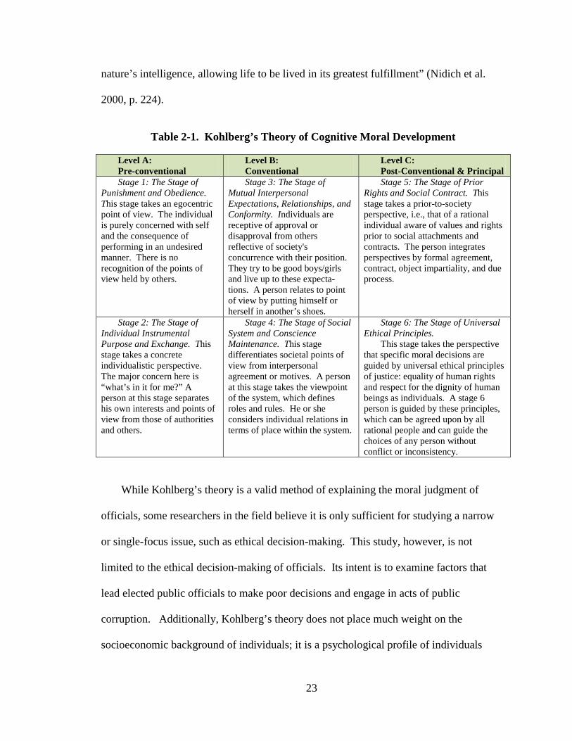
time and place” (Kohlberg 1973a, p. 220 [Table I]). CMD, as presented in Table 2-1

below, is a comprehensive detailing of various stages in which individual behavior is

used to predict moral decision-making. The table outlines the stages a person goes

through according to CMD; these six stages, as presented by Kohlberg, delineate the

expected reactions, behaviors, and rationales that individuals use when presented with

various situations.

Simply stated, research shows that CMD supports the premise that the “development

of higher states of consciousness results in the actualization of all ‘levels of the mind,’

and provides us with the ability to think and act spontaneously in accord with all the laws

of nature, so that our thoughts and actions are fully life-supporting for society and

ourselves. At the highest level of consciousness, unity consciousness, cognitive

development becomes complete with the ultimate identity of human intelligence with

23

nature’s intelligence, allowing life to be lived in its greatest fulfillment” (Nidich et al.

2000, p. 224).

Table 2-1. Kohlberg’s Theory of Cognitive Moral Development

Level A: Pre-conventional

Level B: Conventional

Level C: Post-Conventional & Principal

Stage 1: The Stage of Punishment and Obedience. This stage takes an egocentric point of view. The individual is purely concerned with self and the consequence of performing in an undesired manner. There is no recognition of the points of view held by others.

Stage 3: The Stage of Mutual Interpersonal Expectations, Relationships, and Conformity. Individuals are receptive of approval or disapproval from others reflective of society's concurrence with their position. They try to be good boys/girls and live up to these expecta-tions. A person relates to point of view by putting himself or herself in another’s shoes.

Stage 5: The Stage of Prior Rights and Social Contract. This stage takes a prior-to-society perspective, i.e., that of a rational individual aware of values and rights prior to social attachments and contracts. The person integrates perspectives by formal agreement, contract, object impartiality, and due process.

Stage 2: The Stage of Individual Instrumental Purpose and Exchange. This stage takes a concrete individualistic perspective. The major concern here is “what’s in it for me?” A person at this stage separates his own interests and points of view from those of authorities and others.

Stage 4: The Stage of Social System and Conscience Maintenance. This stage differentiates societal points of view from interpersonal agreement or motives. A person at this stage takes the viewpoint of the system, which defines roles and rules. He or she considers individual relations in terms of place within the system.

Stage 6: The Stage of Universal Ethical Principles.

This stage takes the perspective that specific moral decisions are guided by universal ethical principles of justice: equality of human rights and respect for the dignity of human beings as individuals. A stage 6 person is guided by these principles, which can be agreed upon by all rational people and can guide the choices of any person without conflict or inconsistency.

While Kohlberg’s theory is a valid method of explaining the moral judgment of

officials, some researchers in the field believe it is only sufficient for studying a narrow

or single-focus issue, such as ethical decision-making. This study, however, is not

limited to the ethical decision-making of officials. Its intent is to examine factors that

lead elected public officials to make poor decisions and engage in acts of public

corruption. Additionally, Kohlberg’s theory does not place much weight on the

socioeconomic background of individuals; it is a psychological profile of individuals

24

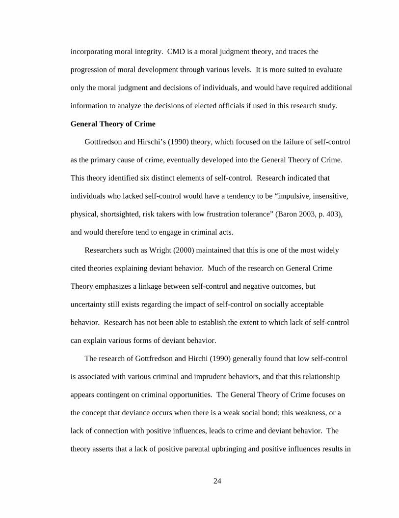
incorporating moral integrity. CMD is a moral judgment theory, and traces the

progression of moral development through various levels. It is more suited to evaluate

only the moral judgment and decisions of individuals, and would have required additional

information to analyze the decisions of elected officials if used in this research study.

General Theory of Crime

Gottfredson and Hirschi’s (1990) theory, which focused on the failure of self-control

as the primary cause of crime, eventually developed into the General Theory of Crime.

This theory identified six distinct elements of self-control. Research indicated that

individuals who lacked self-control would have a tendency to be “impulsive, insensitive,

physical, shortsighted, risk takers with low frustration tolerance” (Baron 2003, p. 403),

and would therefore tend to engage in criminal acts.

Researchers such as Wright (2000) maintained that this is one of the most widely

cited theories explaining deviant behavior. Much of the research on General Crime

Theory emphasizes a linkage between self-control and negative outcomes, but

uncertainty still exists regarding the impact of self-control on socially acceptable

behavior. Research has not been able to establish the extent to which lack of self-control

can explain various forms of deviant behavior.

The research of Gottfredson and Hirchi (1990) generally found that low self-control

is associated with various criminal and imprudent behaviors, and that this relationship

appears contingent on criminal opportunities. The General Theory of Crime focuses on

the concept that deviance occurs when there is a weak social bond; this weakness, or a

lack of connection with positive influences, leads to crime and deviant behavior. The

theory asserts that a lack of positive parental upbringing and positive influences results in

25

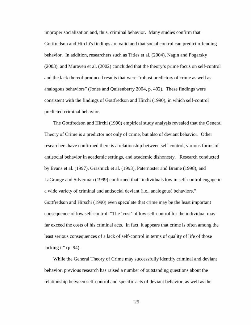
improper socialization and, thus, criminal behavior. Many studies confirm that

Gottfredson and Hirchi's findings are valid and that social control can predict offending

behavior. In addition, researchers such as Titles et al. (2004), Nagin and Pogarsky

(2003), and Muraven et al. (2002) concluded that the theory’s prime focus on self-control

and the lack thereof produced results that were “robust predictors of crime as well as

analogous behaviors” (Jones and Quisenberry 2004, p. 402). These findings were

consistent with the findings of Gottfredson and Hirchi (1990), in which self-control

predicted criminal behavior.

The Gottfredson and Hirchi (1990) empirical study analysis revealed that the General

Theory of Crime is a predictor not only of crime, but also of deviant behavior. Other

researchers have confirmed there is a relationship between self-control, various forms of

antisocial behavior in academic settings, and academic dishonesty. Research conducted

by Evans et al. (1997), Grasmick et al. (1993), Paternoster and Brame (1998), and

LaGrange and Silverman (1999) confirmed that “individuals low in self-control engage in

a wide variety of criminal and antisocial deviant (i.e., analogous) behaviors.”

Gottfredson and Hirschi (1990) even speculate that crime may be the least important

consequence of low self-control: “The ‘cost’ of low self-control for the individual may

far exceed the costs of his criminal acts. In fact, it appears that crime is often among the

least serious consequences of a lack of self-control in terms of quality of life of those

lacking it” (p. 94).

While the General Theory of Crime may successfully identify criminal and deviant

behavior, previous research has raised a number of outstanding questions about the

relationship between self-control and specific acts of deviant behavior, as well as the

26

overall scope of the theory. Although there is a rationale for linking self-control to deviant

acts in a generic approach, the theory cannot explain how, if at all, self-control is related to

specific acts of deviance (Jones and Quisenberry 2004). Gottfredson and Hirchi (1990)

suggest that individuals with low self-control are likely to engage in inappropriate

behavior, a speculation that has not been empirically confirmed.

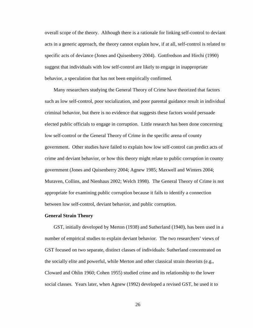
Many researchers studying the General Theory of Crime have theorized that factors

such as low self-control, poor socialization, and poor parental guidance result in individual

criminal behavior, but there is no evidence that suggests these factors would persuade

elected public officials to engage in corruption. Little research has been done concerning

low self-control or the General Theory of Crime in the specific arena of county

government. Other studies have failed to explain how low self-control can predict acts of

crime and deviant behavior, or how this theory might relate to public corruption in county

government (Jones and Quisenberry 2004; Agnew 1985; Maxwell and Winters 2004;

Muraven, Collins, and Nienhaus 2002; Welch 1998). The General Theory of Crime is not

appropriate for examining public corruption because it fails to identify a connection

between low self-control, deviant behavior, and public corruption.

General Strain Theory

GST, initially developed by Merton (1938) and Sutherland (1940), has been used in a

number of empirical studies to explain deviant behavior. The two researchers’ views of

GST focused on two separate, distinct classes of individuals: Sutherland concentrated on

the socially elite and powerful, while Merton and other classical strain theorists (e.g.,

Cloward and Ohlin 1960; Cohen 1955) studied crime and its relationship to the lower

social classes. Years later, when Agnew (1992) developed a revised GST, he used it to

27

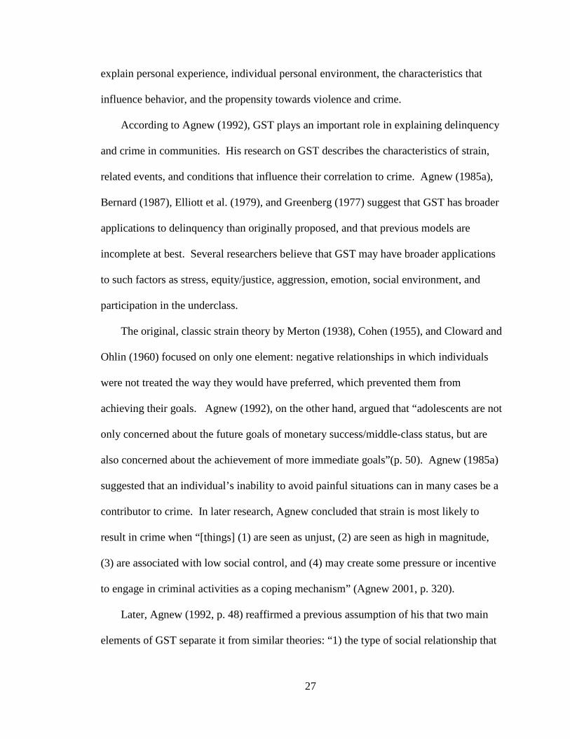
explain personal experience, individual personal environment, the characteristics that

influence behavior, and the propensity towards violence and crime.

According to Agnew (1992), GST plays an important role in explaining delinquency

and crime in communities. His research on GST describes the characteristics of strain,

related events, and conditions that influence their correlation to crime. Agnew (1985a),

Bernard (1987), Elliott et al. (1979), and Greenberg (1977) suggest that GST has broader

applications to delinquency than originally proposed, and that previous models are

incomplete at best. Several researchers believe that GST may have broader applications

to such factors as stress, equity/justice, aggression, emotion, social environment, and

participation in the underclass.

The original, classic strain theory by Merton (1938), Cohen (1955), and Cloward and

Ohlin (1960) focused on only one element: negative relationships in which individuals

were not treated the way they would have preferred, which prevented them from

achieving their goals. Agnew (1992), on the other hand, argued that “adolescents are not

only concerned about the future goals of monetary success/middle-class status, but are

also concerned about the achievement of more immediate goals”(p. 50). Agnew (1985a)

suggested that an individual’s inability to avoid painful situations can in many cases be a

contributor to crime. In later research, Agnew concluded that strain is most likely to

result in crime when “[things] (1) are seen as unjust, (2) are seen as high in magnitude,

(3) are associated with low social control, and (4) may create some pressure or incentive

to engage in criminal activities as a coping mechanism” (Agnew 2001, p. 320).

Later, Agnew (1992, p. 48) reaffirmed a previous assumption of his that two main

elements of GST separate it from similar theories: “1) the type of social relationship that

28

leads to delinquency and 2) the motivation for delinquency.” Reviewing the literature on

GST points up a focus on negative relationships with others, specifically the fact that the

actors in the relationship are not treated as they expect to be treated. Agnew (1992)

suggested that a revised strain theory should include a “relationship in which others

present the individual with noxious or negative stimuli” (p. 49). Agnew (1992), Kemper

(1978), and Morgan and Heise (1988) postulate that individuals are pressured into

deviant behavior by negative affective states, negative emotions like anger and

frustration, and/or negative relationships with others. These negatives create pressure for

corrective action, and crime is one possible response. Agnew (1992) postulated that in

GST, a negative relationship is a result of pressure.

A literature review also shows how Agnew (1984), Elliott and Voss (1974), Elliott et

al. (1985), Empey (1982), Greenberg (1977), and Quicker (1974) have applied strain

theory to various situations in an attempt to predict the likelihood that different types of

strains result in crime and which strains are likely to lead to criminal behavior. Agnew

(1992) stipulated that strain refers to “relationships in which others are not treating the

individual as he or she would like to be treated” (p. 48).

Agnew (2001) identified two different strains, “objective” and “subjective.” He

characterized “objective” strains as the events and conditions disliked by most members

of a given group and “subjective” strains as the events and conditions disliked by the

people who were experiencing or had experienced them. A person under objective

strain(s) is likely to feel pressure to behave in ways most consistent with the group or

culture. That pressure may even motivate the individual to behave in a manner

29

inconsistent with his or her own moral compass. Objective rather than subjective strain is

the focus in this research study.

According to the literature, one area of research attempted to examine individual and

group differences in exposure to external events and conditions likely to cause objective

strain and the subjective review of those events and conditions. Exploring the factors that

influence individual and group differences was vital to the formulation of GST, and is a

major factor in how GST attempts to explain differences in crime between individuals

under objective strain and groups under objective strain.

Agnew (2001) argued that whether subjective or objective strain resulted in criminal

activity was largely a function of the characteristics of the individual experiencing the

strain. He contended that strain is most likely to lead to crime when individuals lack the

skills and resources to cope with their strain in a legitimate manner; that such individuals

tend to have low conventional social support and low social control, and to blame their

strain on others; and, therefore, that such individuals are disposed to criminal behavior.

Supporting research and empirical analyses suggest that perceived or actual social

support from peers, family, and others can reduce negative behavior and assist

individuals in dealing with negative strain (Aneshensel 1992; Cullen 1994; Mirowsky

and Ross 1989; Pearlin 1989).

Agnew (1992) stated that the key factors of GST are based on the actor’s negative

relationships with others. Following this premise, GST contains three types of strains:

(1) a negative relationship with others (individuals or groups) related to the lack of

achieving positively valued goals, (2) the removal (or threat of removal) of positive

30

stimuli, and (3) the threat of being presented with negative stimuli (Langton and Piquero

2007; Agnew 1992).

GST is the theory best suited for this study because each strain suggested by Agnew

(1992) can increase the possibility that “individuals will experience one or more of a

range of negative emotions” (p. 59). Such emotions were critical in judging the behavior

and reactions of elected officials for this study: they include anger, disappointment,

depression, and fear, and according to Agnew (1992), “anger is the most critical

emotional reaction for the purpose of the General Strain Theory” (p. 59). In fact, Agnew

(1992) concluded, “Anger affects the individual in several ways that are conducive to

delinquency. Anger is distinct from many of the other types of negative effects in this

respect, and this is the reason that anger occupies a special place in the General Strain

Theory” (p. 60). Other theorists have supported the role anger plays in GST, and even

proposed that aggression in response to anger is justified (Averill 1982; Berkowitz 1982;

Kemper 1978; Kluegel and Heise 1986; Zillman 1979). Agnew (1992) hypothesized that

“anger results when individuals blame their adversity on others, and anger is a key

emotion because it increases the individual’s level of felt injury, creates a desire for

retaliation/revenge, energizes the individual for actions, and lowers inhibitions”(p. 60).

The literature suggests GST is an appropriate theory for testing the hypotheses of this

research study. For one thing, it offers a broad view of factors that can explain the

behavior of elected county officials who opt to engage in public corruption. These

factors can also identify officials who would desire political acceptance and be more

likely to engage in criminal behavior. According to GST, public officials who lack both

social and economic status may be more inclined to engage in criminal behavior because

31

their lack of acceptance and legitimacy within an elite group can play a critical role in

their decision-making processes. Previous empirical analyses and studies, including

Agnew (1992), have shown that negative strain increases negative emotions, generating

not only anger but also other types of negative behaviors that lead to deviant coping

mechanisms and, possibly, crime. GST is the most appropriate theory to explain public

corruption because it concentrates on the most likely factors contributing to corruption

among elected county officials.

Subcultural Theory

As defined in the Merriam-Webster online dictionary, subculture is “an ethnic,

regional, economic, or social group exhibiting characteristic patterns of behavior

sufficient to distinguish it from others within an embracing culture or society.” Though

subcultures are subordinate to the dominant culture of a society, they sometimes allow

individuals greater group identification; those who take part in particular sports, e.g.,

racing cyclists and professional football players, are sometimes referred to as a

subculture. With this understanding, it is appropriate to suggest that a group of political

representatives who submit to certain social or professional constructs constitutes a

subculture.

Cohen’s Subcultural Theory of deviant behavior emerged from his work on gangs at

the Chicago School, which he developed into a set of theories postulating that certain

groups (or subcultures) in society have preconceived values and feelings that are inclined

towards crime and violence. The theory is largely viewed as a companion to Merton’s

classic strain theory and Cohen himself explained it in similar terms, i.e., as a form of

rebellion. Cohen’s focus, however, was on juvenile delinquency. He and others believed

32

that if the pattern of offenders could be understood and controlled, the cycle of ongoing

criminal behavior from teenage offender into habitual criminal could be broken.

Some researchers suggest that economic needs provoke criminal activity, while

others hypothesize a social-class rationale for deviance. When Cohen (1955) first used

Subcultural Theory to explain deviant behavior, his work concentrated on delinquency

subculture rather than career criminals. Cohen hypothesized that youth delinquents

develop a distinctive culture in response to a perceived lack of economic success and

social opportunity, and that this “status frustration,” as he labeled it, motivated them

toward a life of crime (Cohen 1958). He postulated that the U.S. educational system

instilled a belief in students that they should strive for social status through academic

achievement. If that goal was not attainable for the youth of working-class families,

educational failure would lead to social failure, causing status frustration. Cohen opined

that since working-class youth could not always attain middle-class status, they might

retaliate towards a system that had failed or let them down.

Fischer (1955) concluded that delinquency was not a result of concern for “money

success,” but instead a result of the pressures of all dominant values. Cohen (1958)

suggested that as working-class male adolescents in the inner city fail in school, they

begin to feel they cannot achieve in society by legitimate means and consequently

experience a social status frustration. He argued they form a subculture that “takes its

norms from the larger culture but turns them upside down” (p. 27).

Cohen’s studies validated the hypothesis that lower-class parents instill a different

(from middle-class) value system in their children, with the most important issues being

ones of the moment: food, shelter, and so on. Parents of middle-class youth had

33

significantly different value systems that stressed independence, success, academic

achievement, control of aggression, and respect for property. Cohen (1955) proved that

lower-class youths (and their families) were also more group-oriented and more inclined

to depend on others who shared their value system; their mentality included a feeling of

“watching each other’s back.” The definition of subculture in Fischer (1955)—“a large

set of people who share a defining trait, associate with one another, are members of

institutions associated with their defining trait, adhere to a distinct set of values, share a

set of cultural tools and take part in a common way of life” (p. 544)—best explains

Cohen’s work on Subcultural Theory.

Political figures can exhibit behaviors similar to adolescents; for example, both

groups tend to congregate around individuals who have positions of grandeur. It is not

uncommon for political leaders to engage in social or professional relationships with

wealthy citizens, industry chiefs, celebrities, and other notable figures. Using a

combination of GST and Subcultural Theory, this research study intends to show that

political leaders often feel pressure to live at a standard consistent with the elite groups

that, because of their political position, are now their social peers. When an elected

official’s socioeconomic background and/or current economic conditions cannot support

such a living standard, the official may be tempted to act in ways inconsistent with ethical

expectations as a result of status frustration (negative strain).

When a political leader is found guilty of criminal behavior, the offending act is most

often related to some kind of financial gain. Achieving financial success can provide the

means for a politician to gain legitimacy and permanency within the elite group, whereas

the failure to achieve financial success may result in self-loathing or internal anger. This

34

anger may make the officials who fail more likely to resort to criminal activities, such as

bribery and extortion, as a means of generating additional income to improve their

economic status and acceptance within the elite group. Huntington (1968) and Johnston

(1982) both concur, “corruption is caused by poverty and lack of upward mobility

through legal and socially accepted channels” (Nice 1983, p. 508).

This research study will seek to determine the appropriateness of analyzing

corruption data using the Subcultural Theory, and whether there is a correlation between

GST and Subcultural Theory. The two theories share characteristics germane to

understanding how background, environment, and the desire for social acceptance may

influence elected officials to commit acts of public corruption. The literature review

showed that some researchers assume everyone in a society is initially and consensually

driven towards economic success, wanting to achieve wealth and financial independence.

They propose that this desire for economic success drives some political actors to dismiss

their moral compass, succumb to temptation, and engage in corrupt activities. However,

this research study aims to apply components of GST and Subcultural Theory to the

behavior of elected officials and identify the factors that can induce criminal behavior in

them. Subcultural Theory is associated with a group theory in which people are more

inclined to depend on others who share their value system; while it shares similarities

with GST (e.g., negative strains), it is not as broad as GST and was not a plausible theory

for this research study.

Public Sector Corruption

A review of federal data revealed a continuous annual growth pattern in government

corruption, and insufficient information within the body of literature to explain the

35

increase. In the past 20 years, federal, state, and local officials, as well as private

individuals, have been convicted of government corruption in the United States at an

alarming rate. Public records show that the number of convictions between 1986 and

1995 was 11,888; in the following decade that number nearly doubled, to more than

20,419 convictions. Two likely factors in this increase were the additional staff and the

resources the U.S. Department of Justice brought to bear on the fight against public

corruption in the 1990s.

One case that received widespread attention in 1994 was United States of America v.

McDonough, in which the chairman of the Rensselaer County Democratic Committee

was convicted of receiving more than $500,000 in kickbacks on insurance commissions.

With cases like this in the news, it became imperative for the federal government to

allocate the resources necessary to successfully fight corruption. As authorities realized

the damage corruption could create throughout America, the Justice Department “made it

a priority to target state and local officials for acts of public corruption” (Dreyer 2007, p.

1). More recently, law enforcement officials have focused on developing strict federal

and state laws to fight public corruption. Empirical research, however, suggests that

more stringent laws have done little to reduce the number of officials who violate the

public trust (Maletz 2002; Menzel and Benton 1991).

A review of the literature suggested that one facet of government corruption stems

from the desire of bureaucrats and elected officials for greater social and political

influence, not just more money; however, research has shown that in some corruption

cases, low wages paid to public officials were in fact a motive for corruption. Gould and

Amaro-Reyes (1983), for example, provided evidence that one of the prime causes of

36

corruption is inadequate wages. Another study supporting the notion that low wages may

be an impetus for public corruption was that of Besley and McLaren (1993), who found

that the incentive to accept bribes increased when individuals’ living standards were

squeezed. Given this research, one might conclude that higher salaries would be cost-

effective for government and reduce the potential for public corruption. One function of

this study will be to examine the collected data to determine if low wages in government

jobs can indeed make individuals more prone to corruption (Van Rijckeghem and Weder

2001).

Banerjee (1997) suggested that government has the authority to make it illegal for

bureaucrats to make money using their public position outside of their elected authority.

In fact, governments often try to thwart corruption by creating laws to ensure the public

trust is not violated. Ironically, these laws often create opportunities for corruption by

imposing convoluted regulations on the public. Such rules can complicate the ability to

conduct business quickly and efficiently, and may motivate powerful individuals to

engage in corrupt behavior. Research has shown that corruption often occurs when

elected officials inequitably facilitate the ability to bypass red tape, creating a conflict of

interest (Banerjee 1997).

Overall, the literature review suggested that officials’ corrupt behavior negatively

affects government operations and undermines government functionality. The operating

cost of government is substantially increased and the efficient operation of government is

weakened. According to Transparency International (2005), large bidding and

procurement contracts provide many opportunities to steal money without the public

knowing, and elected officials generally get involved in corrupt activities to enrich

37

themselves or their families and friends. In her book Corruption and Government

Causes, Consequences and Reform, Rose-Ackerman (1999) explored the thesis that there

are conflicts between self-seeking behavior and the public values of public officials. She

argues that self-seeking behavior on the part of government officials compromises their

responsibilities, jeopardizes the integrity of their office, and betrays the very citizens who

elect them.

According to other research studies, “corruption in the public sector results in

inefficiencies in the delivery of public services” (Warren 2004, p. 328). Similar

sentiments are expressed in della Porta and Vannucci (1999, p. 257) and Rose-Ackerman

(1999, p. 9). Corruption provides an unequal playing field to firms who pay bribes to

receive contracts or licenses, preventing officials from selecting the most qualified and

capable bidder. Instead, the firm that offers the highest bribe stands to benefit the most.

The awarding of contracts to unqualified firms because they offer higher bribes, gifts, or

incentives can weaken the stabilization role of government (Tanzi 1998a).

The adverse effects of such activities are not limited to the economics of

government, but can also affect the public services provided to citizens and the financial

strength and stability of government operations. This study will determine the effect

public corruption has on county government, community, the fiscal stability of county

government, and the decisions of public officials. The literature review found that

government corruption erodes the institutional capacity of government; weakens

procedures, rules, and regulations; and siphons off resources that would otherwise be

used for public services. Worst of all, it undermines the legitimacy of government and

erodes public trust. The damage it creates is the main reason the Department of Justice

38

and other law enforcement agencies are concerned about corruption in government, a

view shared by the citizenry. In late 1998, approximately 90 percent of people polled by

the Gallup International Millennium Survey viewed their government as corrupt and

unresponsive to their needs. A government that cannot respond to the needs of its

citizens is weakened to the point of being incapable of governing.

In another research study, Wilson (1960) suggested there might be greater scrutiny of

local officials as the size of local government shrinks and the population becomes more

homogeneous. He argues, “Local voters closely monitor local politicians, because local

politicians’ actions directly affect local tax rates. Further, the display of self-

aggrandizing benefits of local corruption may be obvious to local citizens” (p. 4).

Where corruption among local officials is widespread and institutionalized, local law

enforcement agencies are less likely to fight it. This lack of enforcement amplifies the

environment of corruption (Cabelkova and Hanousek 2004). In a different scenario, if

citizens have adequate proof their officials are engaged in corrupt activities, those

officials’ reelection prospects are likely to be negatively impacted, and the possibility of

losing an election or being removed from office then becomes the justification for

officials to act inappropriately—to seize the opportunity and take advantage of their

office before losing or being removed from it.

The literature suggests that public corruption at the state level, i.e., in the legislative

process, is more likely and occurs more frequently than at the local level. The difference

comes from the differing nature of officials’ political authority and the relationship of the

rules governing the legislature and legislators’ behavior. The state legislative process

“generates incentives for corrupt legislative transactions” (Ackerman 1978, p. 15).

39

Legislators may sell their votes to special interests and lobbyists in exchange for

campaign contributions or other special favors. These favors are often illegal and, as

stated earlier, corrode the public’s faith in political institutions (Lanza 2004). Corruption

at the state level is more common because conflict-of-interest rules are not imposed;

ethics requirements are broad and provide legislators a range of flexibility. Other factors

may include the physical location of the legislature and its accessibility (or lack thereof)

to citizens, a lack of openness and transparency in legislative actions, the access of

lobbyists and special interest groups to legislators, the legislative committee process, and

a legislature that fails to impose restrictions, thereby providing greater opportunities for

corruption.

Corruption at the state level has a history of occurring regardless of how

knowledgeable a constituency is. An increased number of corruption cases over the years

have provided a historical perspective that shows states failing to impose constraints and

these failures creating greater opportunities for a system of corruption at the state level

(Rose-Ackerman 1978). Wilson (1960) argues that state government is more vulnerable

to public corruption than local or federal governments: “States may be more uniquely

prone to corruption: State officials may be subject to less voter scrutiny because each

voter is more poorly informed about the actions of state officials. Further, many state

capitals are located at some geographic distance from the states’ larger metropolitan

areas, which further attenuates press coverage of misdeeds” (p. 3).

Lederman et al. (2004) suggested that political institutions play an important role in

determining the magnitude of the impact of public corruption on government, services,

and the financial stability of government operations. Other researchers have proven that

40

corruption patterns are endogenous to political systems. If laws are not enforced and

rules are not imposed, then corruption persists; but a system of government that is

democratic, open, and transparent is less likely to experience public corruption (Charap

and Harm 1999). Such findings led to the Justice Department’s allocation of the staff and

resources necessary to fight the damage public corruption can create at all levels of

government—federal, state, and local.

Previous researchers have examined a number of factors that contribute to

corruption; however, none of these studies specifically addressed county government.

While other researchers have studied the effects of corruption in areas such as income

distribution, per capita growth, government size, economic stability, discretionary

powers, fair wages, and strength of government, this study seeks to examine the state of

public corruption, the factors contributing to public corruption, and the impact of public

corruption on elected county officials and county government. It will examine whether

government instability, ineffective fiscal management and economic performance,

community characteristics, and the moral characteristics of elected officials contribute to

public corruption within county government. These, along with other factors, deserve

consideration of the impact they have on the decisions of elected county officials to

engage in public corruption.

Elected Officials’ Characteristics and Public Corruption

The literature review suggested that corruption in U.S. politics relates to a

connection between the characteristics of politicians and the elements of corruption. An

analysis of the characteristics of officials and the impact those characteristics have on

corruption was documented in the late nineteenth and early twentieth centuries, and

41

attracted the interest of political scientists in later years. Della Porta (1996) said that to

“understand the emergence and diffusion of corruption it is necessary to look at the

characteristics of the administrators who become involved in corrupt activities” (p. 350).

Other literature surmises that deviant behavior is a byproduct of someone’s environment,

attitude, and social background (Merton 1938; Suther-land 1940; Cloward and Ohlin

1960; Cohen 1955; Piquero and Sealock 2000; Agnew and White 1992; Aseltine et al.

2000; Broidy 2001). GST also suggests that environment, attitude, and social

background can influence behavior and result in an official's decision to engage in

corruption. On the other hand, Agnew (2001a) suggested that conventional success goals

cannot be achieved through criminal activities and do not result in negative strains and

criminal behavior, but this claim is unsubstantiated and does not take into consideration

other important factors related to the demands and failures individuals face.

Some studies suggest that in order to gain a better understanding of the reasons

public officials engage in corrupt behavior, consideration should be given to the

motivation behind their decisions. Money, power, and personal gain are the most

common factors contributing to an official’s decision to engage in corruption, and to

achieve and keep these material benefits, reelection or maintaining the position becomes

the ultimate goal. In essence, a public official's behavior can be motivated by private and

material self-interest.

Previous research has suggested that under GST, an individual's inability to

legitimately achieve success (including monetary success) can result in negative strain

and a decision to engage in illegal activities. Agnew (2001a) points out that there are

different types of strain that may result in criminal activities, and that individuals may

42

attempt “to achieve core goals that are not the results of conventional socialization and

that are easily achieved through crime. Such goals include money, particularly the desire

for much money in a short period of time” (p. 343). The research indicates that offenders

are generally preoccupied with the need for more money. When money becomes the

primary goal of officials, it can create an extreme desire; if money then becomes the core

goal, it forms negative strain and results in deviant behavior.

Further research suggests that another reason public officials engage in corrupt

activities is a perception that the potential benefit may exceed the potential cost (Rose-

Ackerman 1978). In these situations, the perceived benefits and costs of corrupt

activities relate to the values of the official and the expected outcome—and, most

importantly, the probabilities that the outcome is attainable and being caught is unlikely.

Klitgaard (1988) stated it best: “Officials will opt to become corrupt if the benefit of

being corrupt minus the probability of being caught times the penalties for being caught

is greater than the benefit of not being caught”(p. 70). These factors are important

elements associated with the characteristics of elected officials, and weigh in any

decision on whether to engage in corruption.

In another research study, Rogow and Lasswell (1963) proposed that the quest for

power does not necessarily result in public corruption; they hypothesized that

characteristics, upbringing, and environment influence the decisions and behavior of

officials who engage in corruption or acts of personal gain. Wines and Napier (1992)

suggested that cultural values are related to the characteristics of individuals and play

some role in the behavior of individuals engaging in corrupt behavior.

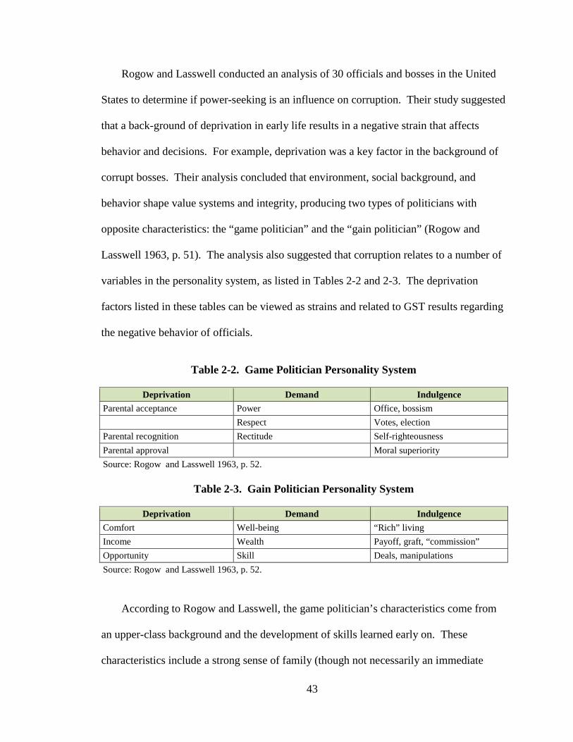
43

Rogow and Lasswell conducted an analysis of 30 officials and bosses in the United

States to determine if power-seeking is an influence on corruption. Their study suggested

that a back-ground of deprivation in early life results in a negative strain that affects

behavior and decisions. For example, deprivation was a key factor in the background of

corrupt bosses. Their analysis concluded that environment, social background, and

behavior shape value systems and integrity, producing two types of politicians with

opposite characteristics: the “game politician” and the “gain politician” (Rogow and

Lasswell 1963, p. 51). The analysis also suggested that corruption relates to a number of

variables in the personality system, as listed in Tables 2-2 and 2-3. The deprivation

factors listed in these tables can be viewed as strains and related to GST results regarding

the negative behavior of officials.

Table 2-2. Game Politician Personality System

Deprivation Demand Indulgence Parental acceptance Power Office, bossism Respect Votes, election Parental recognition Rectitude Self-righteousness Parental approval Moral superiority Source: Rogow and Lasswell 1963, p. 52.

Table 2-3. Gain Politician Personality System

Deprivation Demand Indulgence Comfort Well-being “Rich” living Income Wealth Payoff, graft, “commission” Opportunity Skill Deals, manipulations Source: Rogow and Lasswell 1963, p. 52.

According to Rogow and Lasswell, the game politician’s characteristics come from

an upper-class background and the development of skills learned early on. These

characteristics include a strong sense of family (though not necessarily an immediate

44

closeness), along with civic involvement, discipline, moral virtue and leadership, active

participation in party politics, a college education, and political ambition. They are also

actively involved in the anointment of other political officials. The game politician is a

“man of independent means, who did not exploit politics for personal gain, although the

game politician was privy to innumerable deals which involved the buying and selling of

political favors” (Rogow and Lasswell 1963). He receives glory from building political

kingdoms, controlling power, and influencing his peers. He enjoys the game. The game

politician maintains acquaintances but shares few personal friendships, and receives great

satisfaction from political victories. The game politician has high moral standards.

Game politicians have no interest in corrupt activities for themselves, and do not

compromise their moral standards and ethical rectitude for personal benefit. However,

the game politician has one negative characteristic: he “regarded the uses and abuses of

money in politics as legitimate and he was always willing to arrange matters if at all

possible to promote the financial interest of friends” (Rogow and Lasswell 1963, p. 47).

Rogow and Lasswell characterized the “gain politician” as vastly different from the

“game politician.” The gain politician comes from a poor family background and often

worked as a teenager to help support the family, which was his primary responsibility.

As a young man, he conferred with his mother on important decisions, including political

ones. If an immigrant, he strongly supports the neighborhood political machine. He

develops many friendships within the neighborhood, including some with political bosses

and officials. He gains trust within the organization, and later may create his own

political machine. According to Meier and Holbrook (1992), the prime use of political

machines in urban environments is to benefit the people who support them.

45

The gain politician uses his skills and political acumen for political favors to benefit

his own financial interest; as Rogow and Lasswell (1963) observed, “the [gain politician]

had become the most powerful political boss in the city’s history” and “had also become

one of the wealthiest. The gain politician’s opponents believed—and correctly—that in

the city no contract was let, no tax collected, no post filled, and no facility established

without his extracting a commission” (p. 49). According to Rogow and Lasswell (1963),

the gain politician sees political corruption as a means to compensate for a deprived

upbringing. His primary purpose is personal gain, and politics provides an opportunity to

improve the lifestyle of his family. The personal characteristics of the gain politician

include loyalty to friends and family, generosity, and ambition. The gain politician lacks

high ethical standards and is willing to engage in corruption. The gain politician is less

educated, is not always honest, and lacks moral standards.

Based on a review of the literature, it appears that influence, political control, and

power are the focus for the game politician. This politician appears to be the subject of

“cultural-flaw,” in which lower-class individuals and immigrants maintain enormous

influence through government (Magleby 1984, p. 24). Because of these factors, Rogow

and Lasswell (1963) concluded that the characteristics of elected officials suggest that

corruption is a result of the weakness of individuals (game politician) or a pattern of

politics in which corruption is an acceptable behavior (gain politician).

In a different study, Rivlin (2003) stated that certain characteristics of officials in

both the public and private sectors could pressure them to make inappropriate decisions:

“Successful leaders in both sectors have similar personality traits. They must be

optimistic, competitive, willing to take risks, and able to communicate complex issues

46

understandably” (p. 348). Rivlin goes on to say that the “pressure of complex decisions

in the face of limited information, on the other hand, creates similar ethical dilemmas” (p.

348) and, as a result, individuals can develop “the temptation to shade the truth” (p. 348).

If this happens to public officials, “citizens lose faith in the integrity of public officials,

and democracy becomes at risk” (p. 348). In fact, Rivlin’s analysis focused on the

leadership traits of officials and the general ethical problems they face in controlling the

politics of greed and selfishness.

Meier and Holbrook (1992) proposed that there are historical and cultural

explanations for corruption. They concluded that culture, background, and a lack of

educational attainment can contribute to the behavior of officials, including their

likelihood to engage in corrupt behavior. They also pointed out that corruption in urban

political machines facilitated the rise to power of immigrant groups in the United States

(Greenstein 1964), an element consistent with the characteristics of the gain politician.

Meier and Holbrook (1992) acknowledged that “urban environment[s], in particular,

loosen the social control of family and religion and at the same time concentrate

government programs and resources. In short, urbanism fosters conditions conducive to

corruption” (p. 138).

Researchers have posited that in certain environments, political machines were used

to benefit individuals who supported the machine and were, therefore, considered “part of

the team.” Corruption was the vehicle used to compensate these supporters. Wilson

(1966) supported Meier and Holbrook (1992), saying, “There is a particular political

ethos or style which attaches a relatively low value to probity and impersonal efficiency

and relatively high value to favor, personal loyalty, and private gain” (p. 20). Meier and

47

Holbrook, as well as Wilson, held that the characteristics of elected officials influence

their decisions, and those with certain characteristics would, if given the opportunity,

engage in corruption.

A review of the literature found that “corruption is behavior which deviates from the

formal duties of a public role because of private-regarding (personal, close family, private

clique) pecuniary or status gains; or violates rules against the exercise of certain types of

private-regarding influence” (Nye 1967, p. 419). The possibility exists that certain

characteristics influence the behavior of officials who opt to engage in corruption.

Government Characteristics and Public Corruption

Leff (1964), Huntington (1968), Bardhan (1997), Theobald (1990), Leys (1965), and

Anechiario and Jacobs (1996) all suggest that corruption can have a positive impact on

government by improving efficiency and helping growth. In fact, a common byproduct

of corruption in certain governments is a reduction of burdensome red tape; in such cases,

corruption may be seen as an efficiency measure used by government (Wilson 1989). In

these situations, and in certain countries, corruption is used to bypass burdensome

regulations that slow governmental progress and hamper the function of government, and

to speed up the delivery of services. Corruption through bribery is sometimes called

“speed money” (Azfar et al. 2001, p. 47) because it is viewed as a means of reducing

government inefficiency and speeding up the implementation of policies and regulations.

The literature review suggested various motives to explain the presence of corruption

in the United States. Amundsen (1999) suggested that public corruption exists when

officials systematically abuse laws and regulations and sidestep, ignore, or even tailor

laws to fit their own interests. Johnson (1982) and de Leon (1993) both suggested that

48

public officials with the power to make laws have incentives for corrupt exclusion: they

use the rules and regulations they control to create delays and bottlenecks, and thus are

able to increase the price of their services to bribers. Warren (2004) postulated that the

power elite have no hesitation in using their power and influence to penetrate government

for their personal gain, access government contracts, and influence competition to their

benefit, and in these situations public corruption is likely to occur.

In an environment in which government is inefficient, corrupt bureaucrats are often

provided with “grease money” (Bardhan 1997, p. 1337; Amundsen 1999, p. 11), which

Bardhan considered a benefit to government: “Corruption is the much-needed grease for

the squeaking wheel of a rigid administration” (Bardhan 1997, p. 1322). In many foreign

countries, where government is inefficient and oppressive, bribery is a means to remove

governmental impediments (i.e., red tape) and increase government efficiency (Leff

1964). Indeed, corruption in government was tolerated in many parts of the world until

very recently; in some places, it was even considered the norm. And although Americans

reject corruption, there are countries where public corruption is common practice (e.g.,

South Korea) and does not negatively affect the economy. In many developing nations,

corruption was (and still is) a tolerated practice used to bypass administrative delays.

However, public corruption is not tolerated in the U.S.

Some researchers have argued that corruption may be a good alternative for

improving burdensome and overregulated bureaucratic systems. In these instances,

corruption is viewed as an alternative to an overregulated government and immoderate

resources; however, in the end, corruption harms not only government, but also business

profitability (Amundsen 1999).

49

The U.S. tolerance of corruption virtually ended in the mid-1990s as state and federal

prosecutors made the fight against it a high priority, devoting considerable resources to it.

Although some may view corruption in the developing world as a positive alternative to

overregulated governments, U.S. prosecutors wanted to ensure that corrupt activities did

not become a widespread problem in their nation.4

As government grows, so do the potential rewards of corruption. According to

Johnson (1982), the overall size of a government relates to the possibilities for official

corruption: the larger the government, the greater its spending to support programs and

services. A direct relationship exists between an increase in population and the demands

of citizens for more services, and more money in the system can translate into more

opportunities for corruption.

Another possible factor in corruption is a lack of government accountability.

Without accountability, bureaucrats and elected officials can seize opportunities to

engage in corrupt activities without audits, reviews, or oversight. Stringent accounting

and auditing controls can reduce the potential for corrupt activities as governments use

policies and procedures to ensure that no public officials have overwhelming control or

monopolies over resources. Such accountability measures are an important factor in

fighting corruption within government. Gardiner and Lyman (1978), Rose-Ackerman

(1999), and Transparency International (2000) all suggest governments should provide

assurances that officials will function within specific rules, regulations, and policies that

minimize room for discretionary judgment.

4 Much attention to the cause of corruption gained it prominence among researchers, political

scientists, government officials, economists, and law enforcement officials during this period.

50

Implementing strong ethics laws and pursuing federal prosecutions are powerful

methods for fighting, reducing, or eliminating political corruption within governments.

Rose-Ackerman (1978) suggested that politics can be used to fight corruption if political

actions increase the cost of corruption by increasing the probability that a corrupt

individual will be punished. In addition, officials who are likely to engage in corrupt

activity may become less likely to commit corrupt acts if the threat of being caught is

high (Wilson 1966). In these cases, punishment or removal from office becomes a

concern for officials and affects their decision to engage in corruption.

The review of literature concluded that over the past several years, American politics

and government have seen significant changes that resulted in more opportunities for

graft. According to Williams (1981, p. 29), the “twentieth-century explosion in

government licensing, zoning, regulation, employment and subsidy has provided

unparalleled scope for patronage and graft.” This study will determine the influence of

different variables and the impact they have on the decisions of officials; for instance,

whether a changing society and government structure create varied opportunities for

corruption. The size of government, political uncertainty, a lack of governmental

accountability, increases in government revenues, a lack of public participation,

ineffective ethics, and a lack of law enforcement policies are identified as some of the

potential reasons officials opt to engage in corrupt activities. This study has identified a

number of factors that are influenced by GST and impact the decisions of officials, such

as the tenure of elected officials and salary differentials—two additional variables that

can be related to GST and can influence elected officials’ tendency toward public

corruption. This study will evaluate these factors and determine if there is a correlation

51

between them and public corruption. The study suggests that a correlation exists, but a

definitive decision will be made as this study progresses.

Research suggests that the level of corruption falls when the level of democracy

rises. The more a government provides a legitimate system of governance and functions

within the rule of law, the less likely elected officials are to be involved in corrupt

activities (Amundsen 1999).

Government Economic Performance and Public Corruption

In his book The Effect of Corruption on Growth, Investment and Government

Expenditure: A Cross-Country Analysis, Mauro (1997) provided evidence that corruption

can have considerable adverse impacts on economic performance and delivery of public

services. He further concluded that corruption negatively affects the accountability of

government; therefore, government has a responsibility to address the impact of official

corruption.

One perceived deterrent to corruption in American politics is the development and

stabilization of a robust, economically stable government. The literature review

suggested that as governments and countries grow richer, corruption decreases

(Amundsen 1999); it is reasonable to suggest these same elements apply to county

government. Empirical studies from the World Bank show a strong relationship between

levels of income and corruption, i.e., the higher the income, the lower the level of

corruption (Amundsen 1999; Azfar and Swanmy 2001; Banerjee 1997; Glaeser and Saks

2004; Hunt 2005; Maxwell and Winters 2003; Meier and Holbrook 1992; Williams

2006).

52

Economic distress coupled with growing populations can create pressures on

government. Governments faced with economic uncertainty may become unable to

provide the services and goods needed to keep the community functioning, such as a

good transportation system, public housing, jails, funds for economic development, and

social services. As the population of communities grows, so does the need for

government to provide additional goods and services. The competitive process used to

acquire these goods and services opens the door to corruption, particularly if a

government lacks the resources to monitor the actions of officials in a decision-making

position.

Research further concluded that the system of contracts for goods and services

within government can offer opportunities for corruption. Many of these contracts

provide lucrative opportunities that tempt public officials to engage in corrupt behavior.

Mauro (1997) found that the allocation of public procurement contracts through a corrupt

system led to inferior public infrastructure and services. Corruption in the procurement

process can be very costly for government because it drains funding and reduces

competition; the efficiency of public expenditures decreases as a government is exposed

to corruption.

The research also suggested that corruption is perhaps the most problematic

impediment to a thriving, financially secure government because when “corruption

becomes endemic, it can threaten the basic rule of law, property rights, and enforcement

of contracts” (Azfar et al. 2001, p. 46). Furthermore, corruption is regressive, which

means low-income households bear most of the burden of its costs. Azfar et al. (2001)

53

further states: “This regressive nature of the corruption burden appears to be due to

pervasive corruption in basic public services, education and health” (p. 48).

One of the most harmful consequences of corruption, according to researchers, is the

ambiguity and unpredictability it introduces into business transactions. Mauro (1995)

provided empirical evidence that corruption lowers investment and economic growth;

other researchers found it impedes development by distorting public expenditure

priorities. According to Mauro (1998), it can also lead to the underfunding of critical

services and programs. The premise is that financial stability and sound government may

prevent corruption, which, if not addressed, can destroy county government.

According to Klitgaard (1998), “Corruption is a crime of calculation, not passion” (p.

46). Does a rapid growth in revenues, expenditures, and populations generate more

opportunities for corruption among public officials? Rose-Ackerman (1978) suggested

that it does, and that lax fiscal oversight in a government can prompt officials to engage

in corrupt behavior, particularly if the officials have unlimited flexibility and

discretionary authority to make decisions. Officials who are not governed by a higher

authority, or who have no checks and balances, are likely to engage in corrupt behavior,

and the benefits of doing so become an incentive to only issue contracts to those who pay

the highest bribes.

Officials who oversee the implementation of government regulations, standards, and

programs benefit when standards are vague and unspecific. Such situations provide

prime opportunities for corruption, and can affect the economics of government agencies

by redirecting revenues. In her book Corruption: A Study in Political Economy, Rose-

Ackerman (1978) provides numerous examples of vague guidelines, policies, and

54

regulations, and demonstrates how these elements become factors in corruption

opportunities. Additional elements germane to public corruption are the size of a

government's fiscal responsibilities and a government’s authority and ability to enforce

prudent fiscal policies that protect the financial interests of the public.

The literature review showed that much work is needed for a government to

eliminate corruption and achieve positive economic performance. When this does not

occur, the public often becomes concerned about the negative effect corruption has on

economic performance. Corrupt behavior by public officials for personal benefit destroys

the success of government and its ability to function on behalf of the public. In fact,

according to a survey by Kaufmann (1997), “Elites from across the developing world and

transition economies view public sector corruption as a serious obstacle to economic

development” (p. 125). Corruption, if allowed to persist with limited or no checks and

balances, will divert government funds from needed programs, projects, and community

services to benefit corrupt public officials (Kaufmann 1997).

Community Characteristics and Public Corruption

This study will identify specific factors and pinpoint which indicators from a list of

community characteristics might explain public corruption. Eight indicators of public

corruption will be used: crime rate, population growth, education level of the community,

age of population, civic involvement, poverty, unemployment rate, ratio of county

population to state population, and majority political party of the commission. Which, if

any, of these indicators influence an official to behave corruptly? A series of studies

completed by Johnson (1983), Nice (1983), and Peters and Welch (1980) analyze a

number of factors that help to explain public corruption.

55

Community characteristics, officials’ environment, and social class are not new ideas

for explaining deviant behavior. Theorists such as Agnew, Merton, Cohen, and Cloward

and Ohlin have all studied characteristics they thought could lead to identifying possible

causes of delinquent behavior. These studies appear to be applicable to this research

study, and may aid in identifying what characteristics influence corrupt officials. Do

such factors as social class and community environment influence an official’s behavior

and the propensity to engage in corrupt activities?

The primary discussion for this section of the study will focus on the following

questions: Do social and physical environment influence the behavior and decisions of

public officials? How would the moral character of officials influence their decision to

engage in corruption? Do certain community characteristics play a role in an official’s

corruption? If so, what specific factors actually contribute to officials’ behavior? Which

of these factors, such as social control of family, religion, urbanism, and/or education,

influence a person’s behavior?

Banfield and Wilson (1967) suggested that social class is a factor in the behavior of

officials; middle-class individuals see local politics as a service to the community in

which honesty, efficiency, and impartiality are important factors. They proposed that

social class would more than likely deter middle-class officials from engaging in acts of

public corruption. They also suggested that lower-class individuals would welcome a life

in politics, but would be more likely to engage in public corruption if given the

opportunity. Meier and Holbrook (1992) stated: “Corruption exists because public

service offers individuals a way to become rich that is not available to private citizens”

(p. 146).

56

The literature review suggested that weakness in individuals, if not countered by

strength in the community, can be a factor in an official’s willingness to engage in

corruption. The article “I seen my opportunities and I took ‘em” (Riordon 1963)

succinctly points out that, if given an opportunity, officials will often engage in

corruption, particularly if there are no costs associated with being caught—or if the

benefits of corruption outweigh the cost of punishment.

In the book Power, Corruption, and Rectitude, Rogow and Lasswell (1963)

discussed community characteristics, the environment of public officials, and their social

class, then analyzed how these factors relate to game and gain politicians. The

characteristics of both types are based on environment and social class, the elements of

their background that influenced the decision whether to engage in corrupt behavior. It is

fair to suggest that the characteristics outlined in Rogow and Lasswell (1963) can be

considered an explanation of public corruption, so this section of the research study will

review data to determine the influence community characteristics play in a public

official's decision to engage in public corruption.

57

CHAPTER 3

PUBLIC CORRUPTION IN AMERICA

Historical Framework of Public Corruption

Public corruption has existed in the U.S. since the beginning of the republic, but the

issue attained a new prominence in March 1976 when the Justice Department’s Criminal

Division began a nationwide coordination of federal efforts against corruption at all

levels of government. At the same time, the department created the Public Integrity

Section in the Criminal Division to oversee the prosecution of criminal abuses of the

public trust. The responsibilities of the Public Integrity Section are broad, and include

coordinating the enforcement of all federal statutes related to public corruption.

Congress later passed the Ethics in Government Act of 1978, which requires the U.S.

Attorney General to report annually to Congress on the activities and operations of the

Public Integrity Section. The Act also gave the Attorney General’s Office the

responsibility of consolidating and coordinating the nationwide fight against public

corruption at all levels, including state and local government.

The details of the report provided to Congress each year center on public corruption

cases involving abuses of the public trust by public officials for personal gain. Table 3-1

identifies corruption rankings by state over the past decade, and Table 3-2 lists the top 10

most corrupt states. This data was tabulated by adding total convictions in each state from

2000 to 2009, then identifying the 2009 population for each state to calculate a corruption

rate for each. The corruption rate is defined as the total number of public corruption

convictions from 2000 to 2009 per 100,000 residents. This data involves only federal

public corruption convictions pertaining to federal, state, and local government.

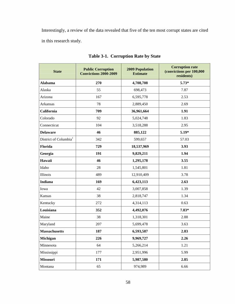
58

Interestingly, a review of the data revealed that five of the ten most corrupt states are cited

in this research study.

Table 3-1. Corruption Rate by State

State Public Corruption Convictions 2000-2009

2009 Population Estimate

Corruption rate (convictions per 100,000

residents)

Alabama 270 4,708,708 5.73*

Alaska 55 698,473 7.87

Arizona 167 6,595,778 2.53

Arkansas 78 2,889,450 2.69

California 709 36,961,664 1.91

Colorado 92 5,024,748 1.83

Connecticut 104 3,518,288 2.95

Delaware 46 885,122 5.19*

District of Columbia1 342 599,657 57.03

Florida 729 18,537,969 3.93

Georgia 191 9,829,211 1.94

Hawaii 46 1,295,178 3.55

Idaho 28 1,545,801 1.81

Illinois 489 12,910,409 3.78

Indiana 169 6,423,113 2.63

Iowa 42 3,007,858 1.39

Kansas 38 2,818,747 1.34

Kentucky 272 4,314,113 0.63

Louisiana 352 4,492,076 7.83*

Maine 38 1,318,301 2.88

Maryland 207 5,699,478 3.63

Massachusetts 187 6,593,587 2.83

Michigan 226 9,969,727 2.26

Minnesota 64 5,266,214 1.21

Mississippi 177 2,951,996 5.99

Missouri 171 5,987,580 2.85

Montana 65 974,989 6.66

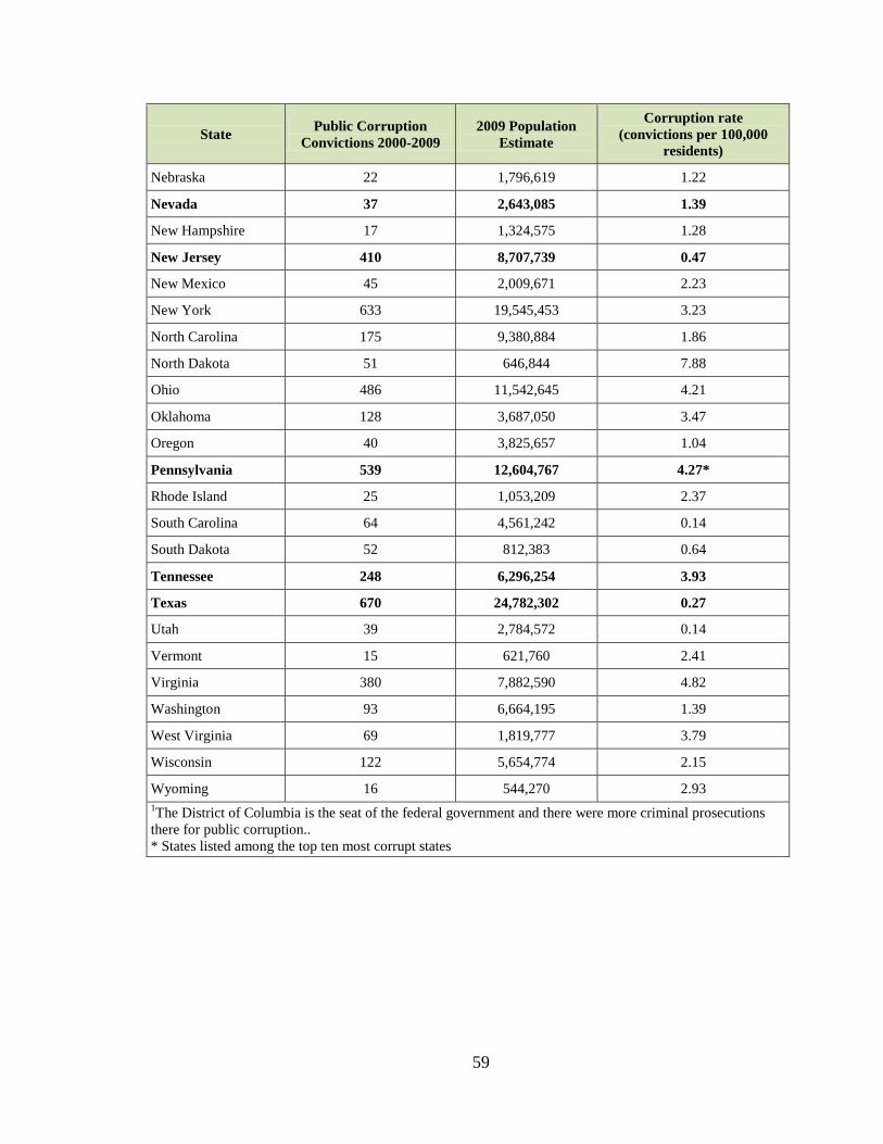
59

State Public Corruption Convictions 2000-2009

2009 Population Estimate

Corruption rate (convictions per 100,000

residents)

Nebraska 22 1,796,619 1.22

Nevada 37 2,643,085 1.39

New Hampshire 17 1,324,575 1.28

New Jersey 410 8,707,739 0.47

New Mexico 45 2,009,671 2.23

New York 633 19,545,453 3.23

North Carolina 175 9,380,884 1.86

North Dakota 51 646,844 7.88

Ohio 486 11,542,645 4.21

Oklahoma 128 3,687,050 3.47

Oregon 40 3,825,657 1.04

Pennsylvania 539 12,604,767 4.27*

Rhode Island 25 1,053,209 2.37

South Carolina 64 4,561,242 0.14

South Dakota 52 812,383 0.64

Tennessee 248 6,296,254 3.93

Texas 670 24,782,302 0.27

Utah 39 2,784,572 0.14

Vermont 15 621,760 2.41

Virginia 380 7,882,590 4.82

Washington 93 6,664,195 1.39

West Virginia 69 1,819,777 3.79

Wisconsin 122 5,654,774 2.15

Wyoming 16 544,270 2.93 1The District of Columbia is the seat of the federal government and there were more criminal prosecutions there for public corruption.. * States listed among the top ten most corrupt states

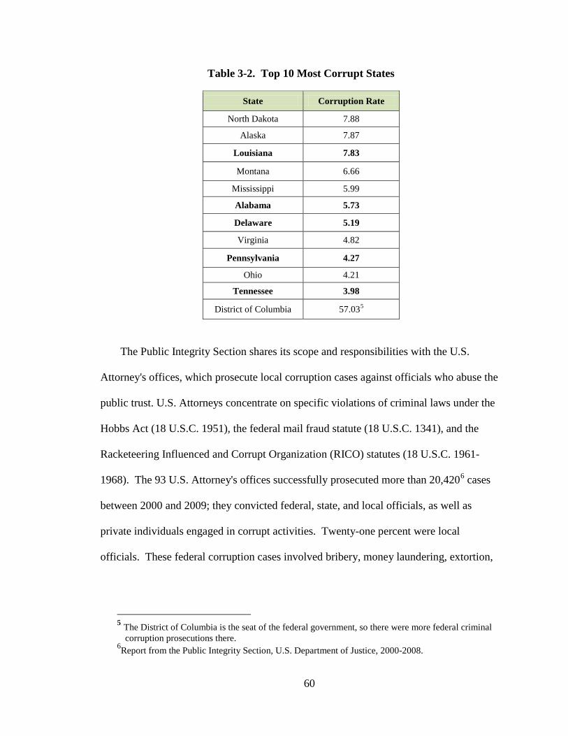
60

Table 3-2. Top 10 Most Corrupt States

State Corruption Rate

North Dakota 7.88

Alaska 7.87

Louisiana 7.83

Montana 6.66

Mississippi 5.99

Alabama 5.73

Delaware 5.19

Virginia 4.82

Pennsylvania 4.27

Ohio 4.21

Tennessee 3.98

District of Columbia 57.035

The Public Integrity Section shares its scope and responsibilities with the U.S.

Attorney's offices, which prosecute local corruption cases against officials who abuse the

public trust. U.S. Attorneys concentrate on specific violations of criminal laws under the

Hobbs Act (18 U.S.C. 1951), the federal mail fraud statute (18 U.S.C. 1341), and the

Racketeering Influenced and Corrupt Organization (RICO) statutes (18 U.S.C. 1961-

1968). The 93 U.S. Attorney's offices successfully prosecuted more than 20,4206

5 The District of Columbia is the seat of the federal government, so there were more federal criminal

corruption prosecutions there.

cases

between 2000 and 2009; they convicted federal, state, and local officials, as well as

private individuals engaged in corrupt activities. Twenty-one percent were local

officials. These federal corruption cases involved bribery, money laundering, extortion,

6Report from the Public Integrity Section, U.S. Department of Justice, 2000-2008.

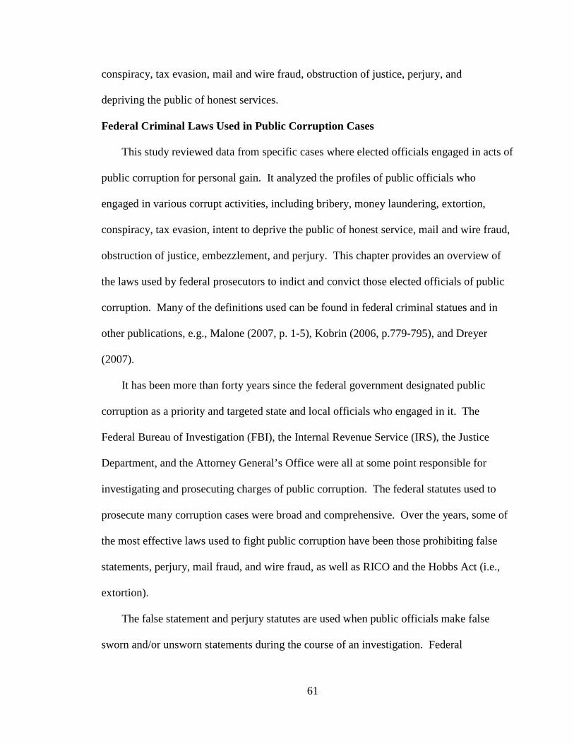
61

conspiracy, tax evasion, mail and wire fraud, obstruction of justice, perjury, and

depriving the public of honest services.

Federal Criminal Laws Used in Public Corruption Cases

This study reviewed data from specific cases where elected officials engaged in acts of

public corruption for personal gain. It analyzed the profiles of public officials who

engaged in various corrupt activities, including bribery, money laundering, extortion,

conspiracy, tax evasion, intent to deprive the public of honest service, mail and wire fraud,

obstruction of justice, embezzlement, and perjury. This chapter provides an overview of

the laws used by federal prosecutors to indict and convict those elected officials of public

corruption. Many of the definitions used can be found in federal criminal statues and in

other publications, e.g., Malone (2007, p. 1-5), Kobrin (2006, p.779-795), and Dreyer

(2007).

It has been more than forty years since the federal government designated public

corruption as a priority and targeted state and local officials who engaged in it. The

Federal Bureau of Investigation (FBI), the Internal Revenue Service (IRS), the Justice

Department, and the Attorney General’s Office were all at some point responsible for

investigating and prosecuting charges of public corruption. The federal statutes used to

prosecute many corruption cases were broad and comprehensive. Over the years, some of

the most effective laws used to fight public corruption have been those prohibiting false

statements, perjury, mail fraud, and wire fraud, as well as RICO and the Hobbs Act (i.e.,

extortion).

The false statement and perjury statutes are used when public officials make false

sworn and/or unsworn statements during the course of an investigation. Federal

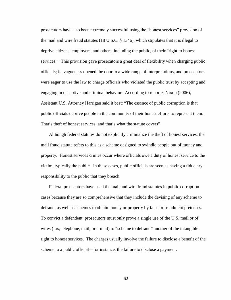
62

prosecutors have also been extremely successful using the “honest services” provision of

the mail and wire fraud statutes (18 U.S.C. § 1346), which stipulates that it is illegal to

deprive citizens, employers, and others, including the public, of their “right to honest

services.” This provision gave prosecutors a great deal of flexibility when charging public

officials; its vagueness opened the door to a wide range of interpretations, and prosecutors

were eager to use the law to charge officials who violated the public trust by accepting and

engaging in deceptive and criminal behavior. According to reporter Nixon (2006),

Assistant U.S. Attorney Harrigan said it best: “The essence of public corruption is that

public officials deprive people in the community of their honest efforts to represent them.

That’s theft of honest services, and that’s what the statute covers”

Although federal statutes do not explicitly criminalize the theft of honest services, the

mail fraud statute refers to this as a scheme designed to swindle people out of money and

property. Honest services crimes occur where officials owe a duty of honest service to the

victim, typically the public. In these cases, public officials are seen as having a fiduciary

responsibility to the public that they breach.

Federal prosecutors have used the mail and wire fraud statutes in public corruption

cases because they are so comprehensive that they include the devising of any scheme to

defraud, as well as schemes to obtain money or property by false or fraudulent pretenses.

To convict a defendent, prosecutors must only prove a single use of the U.S. mail or of

wires (fax, telephone, mail, or e-mail) to “scheme to defraud” another of the intangible

right to honest services. The charges usually involve the failure to disclose a benefit of the

scheme to a public official—for instance, the failure to disclose a payment.

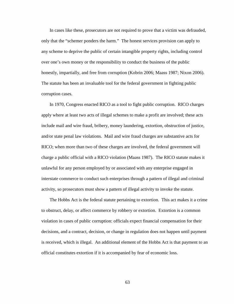
63

In cases like these, prosecutors are not required to prove that a victim was defrauded,

only that the “schemer ponders the harm.” The honest services provision can apply to

any scheme to deprive the public of certain intangible property rights, including control

over one’s own money or the responsibility to conduct the business of the public

honestly, impartially, and free from corruption (Kobrin 2006; Maass 1987; Nixon 2006).

The statute has been an invaluable tool for the federal government in fighting public

corruption cases.

In 1970, Congress enacted RICO as a tool to fight public corruption. RICO charges

apply where at least two acts of illegal schemes to make a profit are involved; these acts

include mail and wire fraud, bribery, money laundering, extortion, obstruction of justice,

and/or state penal law violations. Mail and wire fraud charges are substantive acts for

RICO; when more than two of these charges are involved, the federal government will

charge a public official with a RICO violation (Maass 1987). The RICO statute makes it

unlawful for any person employed by or associated with any enterprise engaged in

interstate commerce to conduct such enterprises through a pattern of illegal and criminal

activity, so prosecutors must show a pattern of illegal activity to invoke the statute.

The Hobbs Act is the federal statute pertaining to extortion. This act makes it a crime

to obstruct, delay, or affect commerce by robbery or extortion. Extortion is a common

violation in cases of public corruption: officials expect financial compensation for their

decisions, and a contract, decision, or change in regulation does not happen until payment

is received, which is illegal. An additional element of the Hobbs Act is that payment to an

official constitutes extortion if it is accompanied by fear of economic loss.

64

The federal government’s use of the extortion statute “under color of official right”

occurs when a public official or private person who has political power receives money

from a third party as a result of the exercise of that power. To qualify as corruption, both

the official and the third party must know or perceive that the official exerted such power

and that the payments were a result of the exercise of official power. Charges against

public officials under the Hobbs Act for obtaining money or property to which they are not

entitled, knowing that a payment was made in return for official acts, are comparable to the

bribery statute.

In fact, the most common violation of public corruption is bribery. A review of

corruption cases indicates that bribery appears to have the highest rate of prosecution of

any form of corruption. It is the classic form of public corruption: individuals or

organizations pay government officials who grant contracts on behalf of a governmental

institution or make decisions on using public funds in order to influence the officials’

decisions on particular contracts or tasks. There are several methods of payments that

constitute a bribe, including kickbacks, payoffs, grease money, and gratuities. Bribery in

corruption cases involves officials who abuse the power entrusted to them by the public

for monetary benefits.

Defining Public Corruption

Government corruption has significant consequences if not reduced or eliminated. To

better explore the topic, this research study must first develop a working definition of it.

Most definitions of public corruption center on the abuse of public office for personal

benefit; this common definition covers the overall behavior of officials using their public

office as a means for personal benefit, and is broad enough to include acts of nepotism and

65

graft. Although the concept of corruption is broad, researchers agree that it generally

refers to acts in which the power of a public office is used for personal gain. Moodie

(1980) said, “Corruption now refers to specific actions by specific individuals—those

holding public positions, elected or appointed, and those who seek to influence them.

Defining corruption becomes a process of spelling out classifications of behavior” (p. 209).

Many researchers have tried to define public corruption; however, the body of

research has yet to produce a consensus on the subject. Klitgaard (1988) says, “[A corrupt

official] deviates from the formal duties of a public role because of private-regarding

(personal, close family, private clique) pecuniary or status gains; or violates rules against

the exercise of certain private-regarding behavior” (p. 23). Ackerman (2001) defines

public corruption as the abuse of one’s public office for personal gain. According to

Georges Bernanos, a French novelist and political writer, “The first sign of corruption in a

society that is still alive is that the end justifies the means”. Another commonly used

definition is that of Nye (1967), who, like Klitgaard, used a definition popular among

political scientists: “[C]orruption is behavior which deviates from the formal duties of a

public role because of private-regarding personal, close family, private clique pecuniary

status-gains: or violates rules against the exercise of certain types of private-regarding

influence” (p. 417). Some economists use a definition from the World Bank (1977): “An

abuse of public office power for private gains.” All these definitions share one common

theme: the misuse of public power for private gain (Senturia 1935, p. 449; Heidenheimer

1989a, p. 9; Key 1936, p. 388; Johnson 1996, p. 331; Benson 1978, xiii; Williams 2006, p.

127).

66

Friedrich (1966) emphasized that a “pattern of corruption can be said to exist

whenever a power holder who is in charge of doing certain things (i.e., who is a

responsible functionary or officeholder) is by monetary or other rewards not legally

provided for, induced to take actions which favor whoever provides the rewards and

thereby does damage to the public and its interest” (p. 74). Amundsen (1999) suggested

that political actors engage in corrupt activities to receive private benefits for themselves,

family, and friends. Bardhan (1997) provides a succinct definition: “Corruption refers to

the use of public office for private gains, where an official (an agent) entrusted with

carrying out a task by the public (the principal) engages in some sort of malfeasance for

private enrichment which is difficult to monitor for the principal” (p. 1321).

Huntington (1968) defines corruption as the “behavior of public officials which

deviates from accepted norms in order to serve private ends” (p. 59). Rogow and Lasswell

(1993) refer to corruption as “behavior in office that is motivated by a desire for personal

material gain” (p. 2). The final definition considered in this research study is offered by

Hutchorft (1996), in which corruption is viewed as a means of payment of bribes by firms

to public officials who, in turn, “expedite a decision without changing it” or “change the

decision and contravene formal government policy” (p. 14).

Each one of these definitions was incorporated into the research, since each relates

corruption to the abuse of public power for personal benefit. Together they contribute to

an overall definition that is broad enough to encompass the overall behavior of officials

involved in corruption, and is thus appropriate for theory building.

67

The final definition comes from Merriam-Webster:

a: impairment of integrity, virtue, or moral principle: depravity

b: decay, decomposition c: inducement to wrong by improper or

unlawful means (as bribery) d: a departure from the original or

from what is pure or correct.

How researchers define corruption determines what data they use to model and

measure it.7 After considering various definitions from the literature, as well as those

offered by previous studies, this research study will use the following definition, slightly

different from the Merriam-Webster one: “The impairment of integrity, virtue, or moral

principle concluding with an inducement to do wrong by improper or unlawful means

relating to governing, a government, or the conduct of government.” With this working

definition of public corruption, this study will delineate two different types: “grand

corruption” and “petty corruption” (Jain 2002, p. 73-75). Grand corruption occurs at the

highest level of government and involves major government programs and projects

(Moody-Stewart 1997). Grand corruption also refers to the acts of political officials who

abuse their position of power to make economic policies for personal use and/or to

preserve their power and wealth (Jain 2001; Amundsen 1999).8

7One sign of the difficulty of defining corruption is that almost everyone who writes about it uses a

different definition. For a brief summary of various definitions, see Jain (1998c, 13-19). For a discussion of the importance of the definition of corruption, see Johnston (2000a), Lancaster and Montinola (1997), and Philil (1997). Collier (1999, p. 4) attributes the absence of a theory of corruption partly to the lack of an agreed-upon definition of corruption. For an earlier attempt to define various types of corruption, see Johnson (1986). Johnson (1996) differentiates between “behavior-classifying” and “principal-agent-client” definitions of corruption.

8“Whoever, having devised or intending to devise any scheme or artifice to defraud, or for obtaining money or property by means of false or fraudulent pretenses, representations of promises, … for the purpose of executing such scheme or artifice or attempting to do so, [uses the mail or causes them to be used], shall be fined not more than $1,000 or imprisoned not more than five years, or both” (18 U.S.C. §1341).

68

Petty corruption occurs at the bureaucratic level, where administrators and appointed

bureaucrats are bribed to fast-track bureaucratic procedures or extort payments while

carrying out tasks assigned to them (Jain 2001; Amundsen 1999). It is most often used to

supplement the income of underpaid bureaucrats. This research focus is grand

corruption.

69

CHAPTER 4

RESEARCH DESIGN AND SYSTEM FOR ANALYSIS

Research Design

The design was a vital component of the overall plan used to explore and analyze

data. The main purpose of a research design is to identify and establish a connection

linking the research questions and the collected data, but another important function is to

provide a road map outlining any prospective links between the researcher’s theoretical

model and the collection and analysis of empirical data.

This research study design is a single-method design that will use a quantitative

research approach to determine if there is a correlation, or cause and effect, between

certain characteristics of elected county officials and their decision to engage in acts of

public corruption. The ladder section of this chapter outlines the research questions and

research hypotheses used to explain the decisions of elected officials.

Design Summary

Model Approach: The research design used a quantitative research approach to

develop and analyze its General Models of Public Corruption.

Model Base: The research design developed assumptions about cause-and-effect

relationships between the dependent and independent variables. The research will seek to

predict and explain relationships between these variables.

Driving Theory: GST was the impetus for the selection of the variables and the

methods of analysis.

70

Description: The research design will describe the data in the study and determine

whether they show a relationship between particular attributes of elected county officials

and public corruption.

Explanatory Aspect: The research study attempts to explain public corruption among

elected county officials who were federally indicted and convicted, as opposed to elected

county officials who opted not to engage in acts of public corruption, using the variables

in the study model. In addition, the study will review data from both areas: those where

there were convictions and those where there were no convictions.

Data Analysis

The analysis will examine data pertaining to county governments with federally

convicted elected officials and county governments with no convicted elected officials.

The analysis will involve a two-stage process. The first stage will be to explain public

corruption in county government. This process includes analyzing 18 variables within

three domains: government characteristics, governmental fiscal characteristics, and

community characteristics. The second stage will be to identify which of the eight

factors within the domain of elected officials' characteristics can best explain the behavior

of elected county officials who engaged in public corruption.

Quantitative Design

Hopkins (1998) states that quantitative research determines how one thing (an

independent variable) affects another (dependent variable) in a population, i.e., it is about

quantifying the relationships between variables. However, the quantitative research

approach is limited in ways that could have some bearing on this research study.

Researchers generally use this approach to ensure that valid statistical methods are

71

applied in the review of data. According to Massey (2003), quantitative design takes no

account of an individual’s lifetime experiences, feelings, and observations. Quantitative

research design is “constructed around a theory, and the theory acts as a systematizing

model for the development of the research questions, hypotheses, data collection

procedure and analyses” (Tekniepe 2007, p. 129). In essence, using a quantitative

research approach is deductive, not only when designing the overall study, but also when

testing the hypotheses and interpreting the results. A quantitative research approach

rejects any opportunity for individual subjectivity, since the results rely on objective

interpretation of data and observations. Therefore, despite its limitations, a quantitative

research approach is the approach best suited for this research study because it removes

any limitations that would affect the outcome of the research analysis.

Unit of Analysis

County commissioners from large urban counties are the focus of this research study.

The unit of analysis was elected county commissioners: those indicted and convicted, and

those not convicted or serving in counties with no incidence of public corruption, in large

urban counties. This unit of analysis is the most appropriate for examining the specific

research questions and hypotheses identified in this study.

Tables 4-1 and 4-2 show that, between 2000 and 2009, 27.74 percent of the

respondents had been indicted or convicted of public corruption in federal court. This

information was used to establish the targeted population.

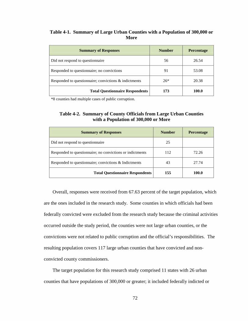
72

Table 4-1. Summary of Large Urban Counties with a Population of 300,000 or More

Summary of Responses Number Percentage

Did not respond to questionnaire 56 26.54

Responded to questionnaire; no convictions 91 53.08

Responded to questionnaire; convictions & indictments 26* 20.38

Total Questionnaire Respondents 173 100.0

*8 counties had multiple cases of public corruption.

Table 4-2. Summary of County Officials from Large Urban Counties with a Population of 300,000 or More

Summary of Responses Number Percentage

Did not respond to questionnaire 25

Responded to questionnaire; no convictions or indictments 112 72.26

Responded to questionnaire; convictions & Indictments 43 27.74

Total Questionnaire Respondents 155 100.0

Overall, responses were received from 67.63 percent of the target population, which

are the ones included in the research study. Some counties in which officials had been

federally convicted were excluded from the research study because the criminal activities

occurred outside the study period, the counties were not large urban counties, or the

convictions were not related to public corruption and the official’s responsibilities. The

resulting population covers 117 large urban counties that have convicted and non-

convicted county commissioners.

The target population for this research study comprised 11 states with 26 urban

counties that have populations of 300,000 or greater; it included federally indicted or

73

convicted elected county officials and those not convicted. The preliminary analysis

found 173 counties with populations of 300,000 or greater, 91 of which had no incidence

of public corruption. The review found nine states had no counties with populations of

300,000 or greater: Alaska, Maine, Mississippi, Montana, North Dakota, South Dakota,

Vermont, West Virginia, and Wyoming (National Association of Counties 2006). These

states were excluded from the research study. In fact, the literature revealed that less than

six percent of the 3,066 counties in the U.S. had populations of 300,000 and greater

(National Association of Counties 2006).

Data Sample

The data and quantitative research observations (sampling) for this research study

were restricted to 117 large urban counties where elected county officials had and had not

been federally indicted and/or convicted of public corruption (based on U.S. District

Court criminal records) between 2000 and 2009. During the data collection process, it

was discovered that 2000–2009 was the period with the most reliable information; earlier

data were sparse, inaccurate, and often unverifiable.

Appendix II lists the large urban counties with public corruption convictions that

were examined for this study, and Appendix III lists the large urban counties with no

cases of public corruption considered. Appendix IV contains the questionnaire used to

obtain information from county governments.

Research Model

Building the model was vital to this study’s overall success. The focus of the study

is the assessment and measurement of the cause-and-effect (predictability) relationship

between the General Models and the domains of elected officials’ characteristics,

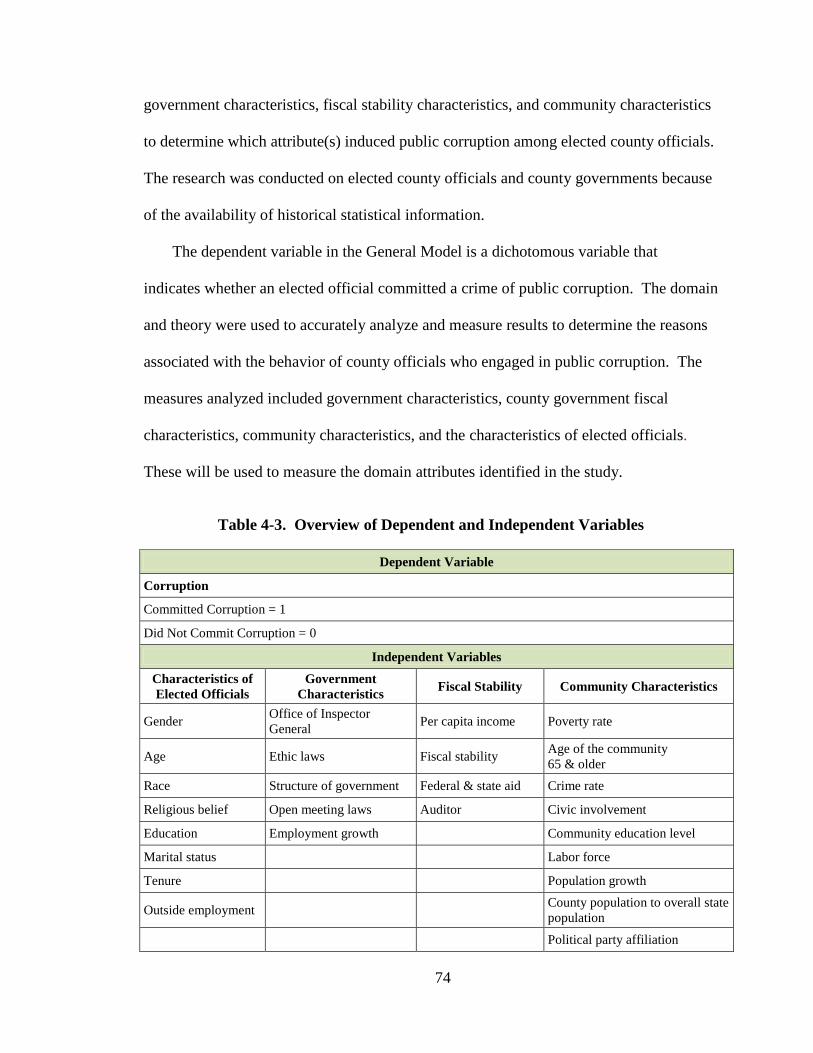
74

government characteristics, fiscal stability characteristics, and community characteristics

to determine which attribute(s) induced public corruption among elected county officials.

The research was conducted on elected county officials and county governments because

of the availability of historical statistical information.

The dependent variable in the General Model is a dichotomous variable that

indicates whether an elected official committed a crime of public corruption. The domain

and theory were used to accurately analyze and measure results to determine the reasons

associated with the behavior of county officials who engaged in public corruption. The

measures analyzed included government characteristics, county government fiscal

characteristics, community characteristics, and the characteristics of elected officials.

These will be used to measure the domain attributes identified in the study.

Table 4-3. Overview of Dependent and Independent Variables

Dependent Variable

Corruption

Committed Corruption = 1

Did Not Commit Corruption = 0

Independent Variables Characteristics of Elected Officials

Government Characteristics Fiscal Stability Community Characteristics

Gender Office of Inspector General Per capita income Poverty rate

Age Ethic laws Fiscal stability Age of the community 65 & older

Race Structure of government Federal & state aid Crime rate

Religious belief Open meeting laws Auditor Civic involvement

Education Employment growth Community education level

Marital status Labor force

Tenure Population growth

Outside employment County population to overall state population

Political party affiliation

75

Data Sampling Process

The independent variables set for individual-level data included eight covariates for

the domain “profile characteristics of elected officials.” Several important factors

associated with this data set are relevant to study analyses. The first is that 43 elected

county officials are included in the research study from 26 large urban counties. The

study identified only those elected officials indicted or convicted on federal charges of

public corruption between 2000 and 2009 who used their elected position for personal

gain; this designation is the main factor for inclusion in the research study. The study

also incorporated 112 elected county officials who were not indicted or convicted of

public corruption charges, but were the counterparts to officials who were corrupt. They

served as members of the county commission during the same period as the county

officials who were indicted and/or convicted, and responded to requests for information.

The process for gathering data from groups of elected county officials—those convicted

or indicted, and their counterparts not involved in acts of corruption—involved mailing

or e-mailing a two-page questionnaire (Appendix IV) and, in some cases, conducting

telephone interviews.

Much of the information for both groups of officials was obtained with the help of

current county commissioners and county staff, state election and ethics department staff,

Justice Department press releases, and the Public Access to Court Electronic Records

service. Collecting data about persons in prison included accessing records through

public information requests at the federal, state, and local government level. Additional

information was gathered from newspaper articles and discussions with news reporters

and staff.

76

A number of former county commissioners no longer on elected boards were located

with the help of county staff and other commissioners. Some officials were still members

of the board, or held another elected position, and responded to the request for

information. In other cases, information was available through county Web sites or

gathered from public record documents. Of the 219 elected county officials who served

as county commissioners during the research period, 180 requests for information were

mailed out to those officials who were located and not deceased. Of the 180 mailed

questionnaires, 155 were completed, returned, and included in the study. The response

rate, over 86 percent, required considerable time and effort in locating accurate

information about the 43 officials indicted or convicted of public corruption, as well as

information pertaining to those officials not convicted. In a few instances, interviews

were conducted with former commissioners convicted of public corruption.

Relational Measures, Data Collection and Sources, and Coding Procedures

This section of the research study describes the functions and specific procedures

used to identify data. It outlines how the research study will address each attribute of the

four domains and how to adequately measure each variable. Exhibit III contains a

concise description of the coding procedures and direction on the types of data gathered

for the dependent and covariates used in the research study. Data was collected from

various sources, both primary and secondary, during a 21-month period that began in

March 2008 and ended in December 2009. Exhibit I provides a summary of the data

sources used for each variable during the data collection process.

77

Quantitative Procedures

Quantitative research is a systematic and objective process that quantifies the

relationship between variables, with the overall purpose of generalizing the information

about the subjects to the overall population. This section will provide an outline of the

methods used in the research study model and a framework for the collection of data.

The study itself incorporates descriptive statistics to summarize the samples and their

measures that describe what the data show and analyze both the dependent variable and

the covariates to determine the relationship between the two variables.

To analyze the cause-and-effect relationship of the independent variables on the

dependent variable, this research study used a logit regression model. The logit

procedure is appropriate because the dependent variable is bivariate with only two

possible outcomes, committed corruption or did not commit corruption, coded

respectively as 1 and 0.

According to Miles and Huberman (2002), the main purpose of regression analysis is

to perform three important functions: (1) prediction, (2) explanation, and (3) control.

Firstly, the regression analysis is used to predict if (and how) the various covariates are

related to the dependent variable—in this case, corruption. Secondly, the logit regression

model is used to explain why certain events happen based on that relationship, and

finally, a regression analysis is used to control for other variables.

The use of a logit regression model in this study allowed testing of the outcomes

from a set of variables that could be dichotomous, discrete, continuous, or a mixture of

any of the three. In the General Models, the dependent variable is dichotomous, while

the independent variables include a mixture. This study will attempt to determine what

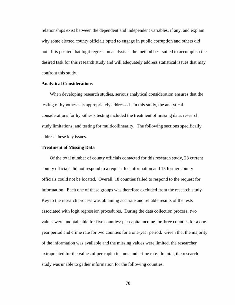
78

relationships exist between the dependent and independent variables, if any, and explain

why some elected county officials opted to engage in public corruption and others did

not. It is posited that logit regression analysis is the method best suited to accomplish the

desired task for this research study and will adequately address statistical issues that may

confront this study.

Analytical Considerations

When developing research studies, serious analytical consideration ensures that the

testing of hypotheses is appropriately addressed. In this study, the analytical

considerations for hypothesis testing included the treatment of missing data, research

study limitations, and testing for multicollinearity. The following sections specifically

address these key issues.

Treatment of Missing Data

Of the total number of county officials contacted for this research study, 23 current

county officials did not respond to a request for information and 15 former county

officials could not be located. Overall, 18 counties failed to respond to the request for

information. Each one of these groups was therefore excluded from the research study.

Key to the research process was obtaining accurate and reliable results of the tests

associated with logit regression procedures. During the data collection process, two

values were unobtainable for five counties: per capita income for three counties for a one-

year period and crime rate for two counties for a one-year period. Given that the majority

of the information was available and the missing values were limited, the researcher

extrapolated for the values of per capita income and crime rate. In total, the research

study was unable to gather information for the following counties.

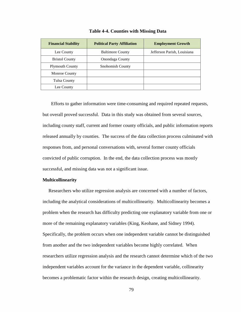
79

Table 4-4. Counties with Missing Data

Financial Stability Political Party Affiliation Employment Growth

Lee County Baltimore County Jefferson Parish, Louisiana

Bristol County Onondaga County

Plymouth County Snohomish County

Monroe County

Tulsa County

Lee County

Efforts to gather information were time-consuming and required repeated requests,

but overall proved successful. Data in this study was obtained from several sources,

including county staff, current and former county officials, and public information reports

released annually by counties. The success of the data collection process culminated with

responses from, and personal conversations with, several former county officials

convicted of public corruption. In the end, the data collection process was mostly

successful, and missing data was not a significant issue.

Multicollinearity

Researchers who utilize regression analysis are concerned with a number of factors,

including the analytical considerations of multicollinearity. Multicollinearity becomes a

problem when the research has difficulty predicting one explanatory variable from one or

more of the remaining explanatory variables (King, Keohane, and Sidney 1994).

Specifically, the problem occurs when one independent variable cannot be distinguished

from another and the two independent variables become highly correlated. When

researchers utilize regression analysis and the research cannot determine which of the two

independent variables account for the variance in the dependent variable, collinearity

becomes a problematic factor within the research design, creating multicollinearity.

80

It is expected that some degree of multicollinearity may occur between covariates,

but how the research resolves the problem speaks to the research design and how well the

research adjusts for issues within the study. After a careful review of covariates, it was

concluded that multicollinearity did not pose a problem in this research.

Research Questions and Hypotheses

The literature review provided a general overview of the impact of public corruption

committed by elected officials, and a possible explanation of their decision to engage in

corrupt activities. Previous research has shown that the activities of officials who engage

in criminal behavior have a negative effect on both private and public institutions; the

literature even emphasizes the profound effects public corruption has had. This is one

reason political scientists and others continue to search for explanations of public

corruption and its negative impact on government operations. As part of that continuing

effort, this study searched for evidence to explain public corruption among county

officials within the past ten years; however, the research suggests that local, federal, and

state governments have experienced explosive growth in corruption cases (United States

Justice Department 2009) which warrants a review of the data.

This study undertakes the task of explaining public corruption committed by elected

county officials, but more importantly, it attempts to shed light on public corruption

Empirical studies by Lederman et al. (2004) imply that political institutions (i.e.,

government) are important in determining the pervasiveness of corruption. Thus, county

characteristics are a vital factor in this research study, and the study will attempt to

explain the impact, if any, that county characteristics have on public corruption. The

study will also attempt to determine if GST or any negative attributes are factors in the

81

behavior of public officials and their decisions to engage in criminal behavior and, if so,

to what degree.

The cause and nature of public corruption among elected officials, particularly

county officials, in contemporary America may be traced to a variety of factors; however,

previous research in this area was unsuccessful in identifying a specific connection to one

or more variables that would explain corruption among elected county officials. The

GST may provide that explanation.

Elected Officials’ Profile Domain

As early as 1963, Rogow and Lasswell noted that an elected official’s profile

characteristics were a determining factor in public corruption. In their book Power,

Corruption, and Rectitude, they identified “game” and “gain” politicians, and it is

through this work that a connection to GST becomes applicable. Rogow and Lasswell

(1963) acknowledged that the personality system in Tables 2-2 and 2-3 delineates three

factors proposed to influence the behavior of elected officials and their decision whether

to engage in corrupt behavior: (1) deprivation, (2) demands, and (3) indulgence. These

three factors, they postulated, can influence elected officials’ decisions and behavior,

shape their ideology and moral character to become corrupt or not. Their study of 30

political officials provided the supporting information used to develop measurable

factors, specific research questions, and hypotheses for the General Models.

To gain a better understanding of the impact of corruption, this research study

examines the characteristics of elected officials and seeks to determine which ones

influence their behavior and decisions. As noted in the literature review, studies by

Langton and Piquero (2007) and other research criminologists, such as Coleman (1995),

82

Croall (2001), and Wheeler (1992), revealed several explanations for white-collar crimes,

including economic pressure, unjust treatment, and personality traits. Their research gave

the confirmation needed to investigate the characteristics of county officials. The goal

was to determine which specific characteristics influenced the decisions of county

officials, and whether the decisions of county officials were made on behalf of citizens or

for personal rewards (della Porta 1996). Mastropaolo (1990) stated, “Career politicians

view politics as a means for achieving upward social mobility” (p. 58-59), leading to this

question: Are the decisions of elected officials reflective of the sentiment of all officials,

and if so, what specific character traits affect behavior?

The decisions of elected officials can be attributed to their upbringing, environment,

failures, and successes. Since GST may provide some explanation of their behavior, it is

an appropriate theory for this study. GST theorizes that behavior and decisions might be

related to three aspects of an official’s environment and upbringing: “1) Their failure to

achieve positively valued goals, 2) removal of positively valued stimuli, or 3) presents of

negative stimuli. Each of these factors, according to research, can influence the decisions

of individuals, and in the case of this research study, is a factor in the behavior of elected

county officials” (Agnew 1992, p. 50). These three factors are measured through (a)

outside employment, (b) age, (c) gender, (d) education, (e) religion, (f) marital status, (g)

race, and (h) tenure. The objective is to determine which of these profile characteristics

are viewed as negative stimuli, which are associated with an official's environment and

background, and whether any of these characteristics are factors in the behavior and

decisions of elected officials. The following subsections present the specific research

83

questions and related hypotheses for the domain of elected officials’ profile

characteristics.

Outside Employment

Research Question 1: What is the relationship between outside employment of

county commissioners and public corruption?

Hypothesis 1: The more opportunities for outside employment that are available, the

more likely it is that county commissioners will engage in public corruption.

It is theorized that a positive correlation exists between outside income (measured as

outside employment) and an elected official’s decision to accept bribes or engage in other

forms of corruption. Outside employment for elected officials includes income or

consulting fees beyond their county commission salaries, i.e., supplemental income.

It is thought that outside employment of county commissioners creates opportunities

in which conflict of interest may occur. Additionally, various types of employment

opportunities can create more chances for a potential conflict of interest and a higher

propensity for public corruption. Therefore, outside employment—specifically, certain

industries or employment opportunities—opens the door to potential problems that

include conflict of interest for elected county officials.

Outside employment is an alternative for improving the financial security of elected

officials, but it is through this avenue that conflict can become an issue. Because county

governments are local in scope, those officials have a greater influence on many aspects

of their communities, including businesses, contracts, zoning, and policies. All of these

elements can directly influence the lives of citizens as well as the business community, so

elected officials of large urban counties generally wield significant power and influence.

84

Consideration should be given to lack of money as one of the fundamental reasons

outside employment is viewed as a precursor to public corruption. A lack of personal

wealth prior to achieving elected office can influence the behavior of county officials,

and once elected, some officials take advantage of any opportunity to engage in corrupt

behavior. A lack of money and power, along with a desire for personal gain, is

hypothesized to be the principal reason to seek outside employment opportunities that

may ultimately lead to political corruption. According to Berg, Hahn, and Schmidhauser

(1976), “Money talks and those who desperately need money are prepared to listen” (p.

41). Their assessment is that lack of money, economic poverty, or a decline in financial

status is a contributing factor of public corruption and a negative strain of GST; the

results of the analysis show these officials perceive a lack of money as a failure to

achieve a positively valued goal. Robert J. Williams’ (2006) assessment of Berg's

analysis is valid: “Despite all the demographic, economic and political changes in this

century, money remains, with apologies to Bagehot, the hyphen which joins, the buckle

which fastens the disparate elements of the American political system” (p. 129).

County government officials are typically compensated, but salaries differ from state

to state and are often inadequate for some officials to maintain a particular lifestyle.

Elected county commissioners who engage in political corruption often have a desire to

maintain a standard of living equal to their peers or business associates within their social

circle, and developing alternative options for generating money becomes important.

Outside employment facilitates the opportunity for officials to engage in corrupt

activities. This study will determine if a relationship exists between those two factors.

GST postulates that outside employment is the venue to resolve the issue of a lack of

85

money, but presents a problem with a conflict of interest and creates situations in which

financial failures stress public officials and result in public corruption. The desire to

generate additional income becomes a factor that can affect decisions (policy and non-

policy), resulting in officials’ decisions that serve to benefit themselves.

According to other studies, there is a relationship between level of income and

corruption. Corruption is low when income levels are high (Amundsen 1999; Van

Rijckeghem and Weder 1997; Swamy et al. 1999; Treisman 1999a; Lipset 1960). GST

postulates that a lack of financial security results in negative strain, and is viewed as a

failure financially and socially. Outside employment opportunities, including

opportunities that create a conflict of interest, provide the vehicle to secure financial

resources and financial security, but have the propensity to result in public corruption.

Age

Research Question 2: What is the relationship between the age of county

commissioners and public corruption?

Hypothesis 2: The more advanced the age of county commissioners, the more likely

they are to participate in public corruption.

It is theorized that a positive correlation exists between county officials’ age

(measured as the age of county officials) and public corruption. The literature review

found empirical studies that examined the relationship between age and public

corruption. The research determined that age is a factor in corruption and can affect the

behavior and decisions of officials. According to previous research, younger officials are

trustworthy and less likely to engage in acts of corruption. In a recent study, Mocan

(2004) showed a correlation between age and corruption. Mocan’s data indicated that

86

younger persons (aged 18 to 20) are less likely to participate in a corrupt act, whereas

individuals between the ages of 20 and 54 are more likely to solicit a bribe. Another

study that suggests an age effect in criminal behavior is Torgler and Valev (2006), which

demonstrated that age influences the criminal behavior of individuals and the decisions

individuals make. This study will examine the ages of officials and seek to determine at

what age elected officials will become involved in corrupt activities, the relationship of

age to corruption, and whether public corruption is associated with an age effect. Under

GST, one might hypothesize that younger public officials desire instant financial success

and are not willing to devote the time to achieve financial and career advancement. This

study will determine if older public officials are typically more financially stable than

younger officials, and if so, whether younger officials would be more likely to develop

financial stress that results in acts of public corruption.

Gender

Research Question 3: What is the relationship between a county commissioner’s

gender and public corruption?

Hypothesis 3: Male county commissioners are more likely than female county

commissioners to engage in public corruption.

It is theorized that a positive correlation exists between the gender of county officials

(measured as the gender of officials) and public corruption. The literature review

discovered studies that examined public corruption and gender (e.g., Azfar et al. 2001).

Where there is a propensity to engage in corruption, the literature showed that acts by

women were less severe (Swamy et al. 1999; Dollar et al. 1999). The hypothesis,

therefore, is that men have a higher propensity to be involved in acts of corruption than

87

women. Men are more likely to serve as elected officials, but even when women are

elected, their priorities are issue-based. In most cases, women seem more concerned with

solving problems than obtaining power or money.

The literature review found that several countries used an unusual gender-related

policy to confront corruption and reduce corrupt behavior in government: women were

put in leadership and management positions as an anticorruption method (Moore 1999;

McDermott 1999). Studies have found that women and men approach corruption

differently, and evidence suggests that women commit lower levels of criminal activities

than men (Torgler and Vale 2007). There is also evidence of gender differences on

ethical decision-making (Ford et al. 1994; Glover et al. 1997; Reiss & Mitra 1998):

studies suggest there are higher degrees of ethical standards governing women’s behavior

than men’s, and that “in the short run, a greater presence of women in public life will

reduce corruption” (Azfar et al. 2001, p. 53).

This research study will examine the data to determine if a valid explanation exists

that can explain why more incidents of public corruption are committed by men than by

women.

Education

Research Question 4: What is the relationship between the education of county


Hypothesis 4: The higher the level of education among county commissioners, the

less likely it is a commissioner will engage in public corruption.

It is hypothesized that a negative correlation exists between county officials’

educational achievement (measured as county officials’ level of education) and public

88

corruption. A review of the literature found no specific studies that have examined the

relationship between the level of formal education and public corruption; however, it is

hypothesized that elected county officials who have advanced degrees are less likely to

participate in corrupt activities than their counterparts who do not. According to Torgler

and Dong (2008), one study prepared by Mocan (2004) suggested that “higher levels of

education can lead to a higher probability of being targeted for bribes, stressing also that

a more educated population is expected to be less tolerant of corruption” (p. 14).

Although elected officials with a high level of education may be targets for those

behaving illegally, it is posited that elected officials will be less apt to participate in such

behavior if they have advanced degrees. This research study will examine education and

public corruption to determine if a correlation exists between public officials’ level of

education and their willingness to engage in corrupt activities.

GST postulates that “educational attainment is referred to as a mark of social status

and thus believed to indicate a greater stake in conformity; poor academic performance

was likely to result in greater stress for a white-collar offender than for the common

criminal” (Langton and Piquero 2007, p. 5). It is theorized that county officials who

failed to achieve educational success may view public corruption as an opportunity to

advance to the status level of their peers. This assessment would lead one to believe that

a large number of highly educated elected officials would result in a lower level of

corruption in government.

Race


ethnicity and public corruption?

89

Hypothesis 5: White county commissioners are less likely to engage in public

corruption than other commissioners.

It is hypothesized that a positive correlation exists between non-white commissioners

(measured as the race of county officials) and public corruption. The literature review

found several studies that investigated the relationship between corruption and ethnic

heterogeneity; in literature broadly concerned with ethnicity and corruption research,

studies revealed a possible relationship between corruption and ethnic diversity (Mauro

1995; Alesina, Bagir, and Williams 2002; La Porta et al. 1999). In fact, according to one

study by Mauro (1995), “The presence of many different ethnolinguistic groups is also

significantly associated with worse corruption, as bureaucrats may favor members of

their same group” (p . 693).

It is hypothesized that a county official’s race is a relevant factor in the discussion of

public corruption in county government, and that race can influence an official’s behavior

and decision-making ability. Race is a negative element that creates social rejection for

officials. According to Jang and Johnson (2003), Hagan and Peterson (1995), Mirowsky

and Ross (1989), Ross and Van Willingen (1996), and Schulz et al. (2000), race is a

negative strain and could cause non-white officials “psychological distress due to their

more frequent experiences of racism and economic disadvantage” (p. 83). Empirical

evidence confirms that GST can apply to people of color, particularly African-

Americans, who have experienced a greater level of strain due to racism, economic

disadvantage, prejudice, and unfair treatment. The literature review suggested that

African-Americans may externalize adversity, which could be related to years of harsh

treatment and in the end result in the development of racial consciousness (Neighbor et

90

al. 1996).9

A review of Meier and Holbrook (1992) showed that a larger number of minority

elected officials were investigated for corruption and targeted for prosecution, but there is

a lack of supporting evidence for the conclusion that minorities engage in political

corruption at a higher rate than non-minorities. This study will examine the data to

determine if corruption is greater among minorities. It is also thought that the impact of

corruption is affected by the race of officials because “ethnic fragmentation impacts

corruption by reducing the popular will to oppose politicians. If an area is torn apart by

ethnic divisions, leaders tend to allocate resources towards backers of their own ethnicity,

then members of one ethnic group might continue to support a leader of their own ethnic

group, even if he is known to be corrupt” (Glaeser and Saks 2004, p. 5-6).

This research study will examine race to determine if levels of corruption are

greater among minorities. GST will be used to analyze data to determine if a correlation

exists between the race of county officials and corrupt behavior.

Religion

Research Question 6: What is the relationship between the religion of county


Hypothesis 6: County commissioners with religious beliefs are less likely to engage

in public corruption.

It is thought that a negative correlation exists between the degree of devotion to a

religion among county commissioners (measured as county officials’ public display of

faith) and public corruption. According to Lambsdorff (1999), “A strong association

between religion and corruption is obtained by Treisman [1999a]” (p. 11). Additionally,

9 Neighbor et al. defined racial consciousness as “a set of beliefs about relative position of African-Americans in society.

Specifically, consciousness is a collective interpretation of personal experience that includes power grievances about a group's relative disadvantaged status, which influences blacks to keep stress external rather than allowing it to become internalized” (171).

91

La Porta et al. (1997), Treisman (1999a), and Paldam (1999b) theorize that the role of

religion in an official’s life contributes to the level of corruption. The research conducted

by La Porta et al. found “that such hierarchical form of religion is detrimental to civic

engagement, a factor which should help reduce corruption” (Lambsdorff 1999, p. 11).

Torgler (2006) suggests that engagement in illegal activities might be affected by

people’s religious involvement, and that there may be a relationship between religion and

the behavior of elected officials. Other research suggests that religion has a positive

effect on GST, and that religion is a social connection and strength for families and

individuals. According to Piquero and Sealock (2000) and Jang and Johnson (2003),

spiritual or religious factors may shield the effects of negative emotions, reduce deviant

coping, and decrease the effect of strain. This study will review religion as a factor and

determine its influence on corruption.

Marital Status


marital status and public corruption?

Hypothesis 7: County commissioners who are not married are more likely to engage


It is thought that a positive correlation exists between the marital status of county

commissioners (measured as the marital status of county officials) and public corruption.

A review of the literature found some information indicating that marriage could have an

effect on elected officials’ behavior. Swamy et al. (2001) held that marriage can alter

public behavior, while a criminal study by Gottfredson and Hirschi (1990) theorized the

opposite—that marital status has no influence on the likelihood of crime. GST postulates

92

that elected officials who are divorced can experience negative emotions, including

anger, which reflect their social status and can influence their public life, i.e., failure in

marriage can create a perception of failure in other aspects of public life. A divorce

while in public office can negatively reflect on the performance and abilities of public

officials, and stressful tension in public life may affect the decisions of individuals. This

research study will explore the relationship to determine if a correlation exists between

the marital status of county officials and public corruption.

Tenure


tenure in public office and public corruption?

Hypothesis 8: County commissioners with fewer years on the county commission are

more likely to engage in public corruption.

It is theorized that a positive relationship exists between a lengthy tenure of elected

office (measured as the number of years in office as a county official) and public

corruption. The literature review found no studies that addressed a relationship between

public corruption and tenure, and it is generally believed that tenure has no influence on

the behavior and actions of public officials. However, this study will review data to

determine if there is a relationship between the length of time in public office and the

decision of public officials to engage in corruption.

The length of time an official remains in office speaks to that official’s stability. It is

hypothesized that the tenure of elected officials can affect their ability to make sound

decisions and value judgments. It seems likely that county officials who seek to climb

the political ladder rapidly would be more inclined to take every opportunity for political

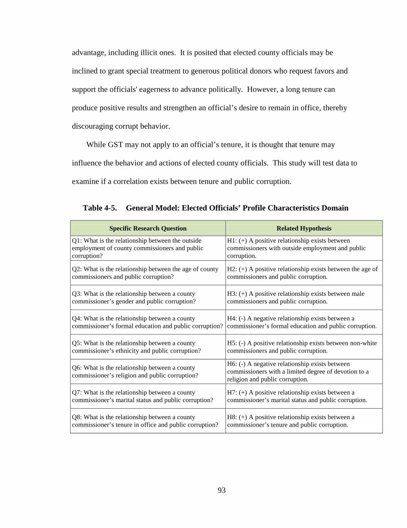
93

advantage, including illicit ones. It is posited that elected county officials may be

inclined to grant special treatment to generous political donors who request favors and

support the officials' eagerness to advance politically. However, a long tenure can

produce positive results and strengthen an official’s desire to remain in office, thereby

discouraging corrupt behavior.

While GST may not apply to an official’s tenure, it is thought that tenure may

influence the behavior and actions of elected county officials. This study will test data to

examine if a correlation exists between tenure and public corruption.

Table 4-5. General Model: Elected Officials’ Profile Characteristics Domain

Specific Research Question Related Hypothesis

Q1: What is the relationship between the outside employment of county commissioners and public corruption?

H1: (+) A positive relationship exists between commissioners with outside employment and public corruption.

Q2: What is the relationship between the age of county commissioners and public corruption?

H2: (+) A positive relationship exists between the age of commissioners and public corruption.

Q3: What is the relationship between a county commissioner’s gender and public corruption?

H3: (+) A positive relationship exists between male commissioners and public corruption.

Q4: What is the relationship between a county commissioner’s formal education and public corruption?

H4: (-) A negative relationship exists between a commissioner’s formal education and public corruption.

Q5: What is the relationship between a county commissioner’s ethnicity and public corruption?

H5: (-) A positive relationship exists between non-white commissioners and public corruption.

Q6: What is the relationship between a county commissioner’s religion and public corruption?

H6: (-) A negative relationship exists between commissioners with a limited degree of devotion to a religion and public corruption.

Q7: What is the relationship between a county commissioner’s marital status and public corruption?

H7: (+) A positive relationship exists between a commissioner’s marital status and public corruption.

Q8: What is the relationship between a county commissioner’s tenure in office and public corruption?

H8: (+) A positive relationship exists between a commissioner’s tenure and public corruption.

94

Community Characteristics Domain

Community characteristics are another set of factors thought to affect public

corruption among elected officials. It is posited that the demographics and environment

of a community can influence county officials’ behavior. Several research studies

indicate that the characteristics of a community and the community’s environment for

politicians could have a great deal to do with an official’s conduct, decisions, and

behavior (della Porta 1996; Hunt 2004; Maxwell and Winters 2003; Meier and Holbrook

1992; Menzel and Benton 1991). In addition, an official's peers, community, friendships,

teachers, religious influences, and families are all nurturing elements that can become

factors in both actions and conduct.

This study analyzes community characteristics as an important determinant of the

corruption of county officials. It considers the relationship between a number of

community factors, including poverty rate, level of college education, percentage of the

community aged 65 years or older, level of civic involvement, and population of the

county. The study examines how community characteristics affect a politician’s

decisions, as well as how they shape that person’s social class, values, moral character,

and beliefs, and what influence these may have on a decision to engage in public

corruption.

This research study will investigate whether community environment influences the

decision-making processes of officials. Do the negative attributes of a community

influence the behavior of officials, and are these factors enough to result in negative

strains on an official? It has already been theorized, and previous research suggests, that

individuals experiencing negative emotions, displeasures, stress, and a lack of social

95

acceptance/status may more readily engage in corrupt activities (Jang and Johnson 2003;

Langton and Piquero 2007; Nas, Price, and Weber 1986; Warren 2004). The

corresponding question for this domain is: Can the negative attributes of a community

also result in an official’s decision to engage in public corruption?

A review of the literature suggests that there is a relationship between community

environment and the corruption of elected officials. GST is a possible explanation of,

and could be a contributing factor to, the behavior of elected officials who engage in

corrupt activities. In recent years, many citizens have become concerned about the

negative influence of corruption on communities. Since there is little research explaining

why corruption exists and, more importantly, why it is more prevalent in some

communities than others, this research study will examine possible differences in

corruption based on the community and whether one’s social class may influence the

decision to engage in public corruption. The objective is to determine the circumstances

in which community characteristics influence public corruption. The study will try to

determine if factors such as crime, poverty rate, and general age of the community in

larger urban counties provide greater opportunities for corruption.

The research study sets forth eight attributes to measure the domain of community

characteristics: (a) poverty rate, (b) crime rate, (c) civic involvement, (d) secondary

education level, (e) labor force, (f) age of the community, (g) county population growth,

(h) ratio of county population to overall state population, and (i) political party affiliation.

The objective is to identify community characteristics that might influence negative

behavior and the decisions of elected officials to engage in acts of public corruption.

96

Poverty Rate

Research Question 9: What is the relationship between the poverty rate of

communities and public corruption?

Hypothesis 9: Impoverished communities are more likely to experience public

corruption.

It is hypothesized that a positive correlation exists between high poverty rates

(measured as poverty rate for the county) and public corruption. It is thought that a

community with a high poverty rate indicates that citizens are not likely to scrutinize the

decisions and behavior of elected officials because they lack the time and attention to

serve as government watchdogs. In some cases, these citizens also lack the education and

sophistication to monitor and understand the mechanics and workings of government.

Hunt (2004) suggests that poor citizens are less likely to engage in giving bribes and are

more likely to be harmed and excluded from public services, while “the rich pay the most

in bribes” (p. 3) and have a better understanding of the mechanics of government. It is

thus posited that the poverty rate can provide an indication of public corruption.

Additionally, poverty rates among communities are a negative strain and are related to

GST. Public officials who have experienced, or reside in, an environment of poverty are

more likely to experience negative strains, and many experience other failures throughout

their lives. The influence of poverty on communities can ultimately affect the behavior

of officials; if officials reside in a community with a high rate of poverty, strains are

likely to exist. Two possible negative factors come from high poverty rates and GST:

inadequate financial status and poor living conditions. Both in this case are negative

97

strains. The study seeks to determine if negative strains create an environment for

corruption.

Crime Rate

Research Question 10: What is the relationship between communities’ crime rate

and public corruption?

Hypothesis 10: Communities with high crime rates will see more cases of public

corruption.

It is hypothesized that a positive correlation exists between the crime rate (measured

as violent crime per 100,000 inhabitants in the county in any one-year period) and public

corruption. Nice (1983) suggests that “political corruption is merely the extension of

private behavior in the public realm and that the crime rate should be a good surrogate for

tolerance of corruption” (p. 509). Further research suggested that crime creates a lack of

trust, and lack of trust opens the door to an environment of criminal behavior by

government officials (Hunt 2004, p. 22). Meier et al. (1992) and Hunt (2004) suggest that

a high crime rate is an indicator of the political system’s inability to address the issue of

crime, and that communities with high crime rates do little to reduce crime or implement

policies and penalties stringent enough to deter crimes such as public corruption.

Schlesinger and Meier (2002) found that public corruption and the crime rate within

communities are linked, and “it is expected that corruption would be lower in states

where a larger proportion of the population feels it is important to obey the law because

of moral principles. In addition to being an ethical issue, corruption is also considered a

crime” (Morris 1991, p. 11). Researchers, however, suggest that high crime rates in

communities are an indication that the political system is unable to address the issue of

98

crime, implement effective law enforcement policies and penalties, and/or develop

effective policies to reduce public corruption (Meier and Holbrook 1992). Research also

revealed that larger communities have more oversight by law enforcement agencies and

more effective policies to address corruption in local government. Larger communities

also tend to have more resources to combat crime.

Civic Involvement

Research Question 11: What is the relationship between the civic involvement of

communities and public corruption?

Hypothesis 11: Communities with less civic involvement will have more cases of

public corruption.

It is theorized that a negative correlation exists between civic involvement (measured

as voter turnout) and public corruption. It is thought that citizens who show high levels

of civic involvement in the political process by participating in elections are more

engaged in the activities and decisions of government officials, and are more willing to

attend meetings and demand transparency from government. The research also suggests

that the more citizens are politically involved, the less likely they are to tolerate the

presence of corruption. Hence, the decisions of officials become more judicious.

Community Post-Secondary Education Level

Research Question 12: What is the relationship between a higher education level

of the community and public corruption?

Hypothesis 12: The greater the post-secondary education level of a community, the

fewer the opportunities for public corruption.

99

It is theorized that a negative correlation exists between higher education (measured

as the post-secondary education of the community) and the reduction of public

corruption. It is thought that citizens with higher levels of post-secondary education are

less tolerant of public corruption by elected officials. The more educated the citizenry is,

the more likely it is that citizens are informed and will question the decisions of county

officials. While it may be argued that elected officials with advanced educational degrees

are less corrupt, Lipset (1960) suggests that communities with higher levels of education

are also less corrupt, a factor this research study proposes to explore. It is thought that

citizens with higher levels of education are more likely to analyze and review information

before final acceptance of decisions by elected officials.

Labor Force

Research Question 13: What is the relationship between the unemployment rates

of communities and public corruption?

Hypothesis 13: The greater the unemployment rate is, more likely there is public

corruption.

It is hypothesized that a positive correlation exists between labor force (measured as

the percentage of the unemployment rate in the county) and public corruption. High

unemployment rates in communities suggest that citizens are more concerned with

seeking employment opportunities and providing for their families than with monitoring

the activities of county officials. It is thought that a high rate of unemployment results in

an unstable community and a higher degree of transience. Individuals may be more

inclined to relocate to communities where employment opportunities are greater.

Additionally, a high unemployment rate could be an indicator for high levels of crime in

100

communities. It is posited that high unemployment in communities would result in

public corruption. Poor communities with a high degree of crime suggest citizens who

are focused on survival, with limited time to watch the activities of government and

elected officials. This would likely result in more opportunities for public corruption.

Age of Community (65 years and older)

Research Question 14: What is the relationship between the age of community

populations and public corruption?

Hypothesis 14: Communities with a higher level of older people are less likely to

experience public corruption.

It is theorized that a negative correlation exists between the age of the community

population (measured as the percentage of the county’s population 65 years and older)

and public corruption. It is thought that citizens who are retired have more leisure time,

and thus opportunity, to monitor government activities through the behaviors and

decisions of their elected officials. In their study of corruption, Menzel and Benton

(1991) theorized that retirees have more wisdom and moral maturation and demand a

higher standard of ethics from officials, while Hunt (2004) found that older people are

less likely to engage in illegal activities and acts of corruption. The moral-development

theory presented by Kohlberg (1976) may apply to older citizens, in that they have a

different perspective and are more concerned with the ethical outlook of elected officials

than younger and middle-age citizens. Indeed, Menzel and Benton (1991) suggested that

senior citizens are more inclined to stop public corruption and wrongdoing by tracking

the actions of elected officials, the behavior of officials, and government spending

patterns. It is posited that, in communities with large populations of older citizens, there

101

is a greater chance that corruption in county government does not occur or occurs to a

lesser degree.

Population Growth

Research Question 15: What is the relationship between a county’s population

growth and public corruption?

Hypothesis 15: The greater the county’s population growth rate, the more likely it

is public corruption will occur.

It is posited that a positive correlation exists between population growth (measured

as one-year change in total population) and public corruption. An increase in population

generates more revenues for county budgets, which results in more expenditures (e.g., for

grants and contracts), hence more opportunities for misappropriation of funds. No

previous research studies have explored the relationship between the level of population

growth and public corruption. It is thought, however, that the more flexibility officials

have to spend newly generated revenues from growth, the greater the opportunity for

misappropriation of funds and, therefore, for elected county officials to engage in corrupt

activities.

Ratio of County Population to State Population

Research Question 16: What is the relationship between the ratio of the county

population to the state population and public corruption?

Hypothesis 16: The greater the ratio of the population of the county to that of the

state, the more likely public corruption is to occur within the county.

It is thought that a positive correlation exists between counties where the majority of

the state’s population resides (measured as the percentage of the county population

102

compared to the state population) and public corruption. While no previous studies have

examined the relationship between the ratio of the county population to the state

population and public corruption, it is thought that corruption is more likely to occur in

large urban counties because they tend to generate the majority of revenues for the state.

Elected officials in large urban counties have greater responsibilities, power, and sense of

privilege or entitlement, which present opportunities to violate the law or engage in acts

of public corruption.

Per Capita Income

Research Question 17: What is the relationship between per capita income and

public corruption?

Hypothesis 17: A high rate of per capita income results in less public corruption.

It is theorized that a negative correlation exists between a county’s per capita income

(measured as the annual per capita income for the county population) and public

corruption. The overall wealth of a community is an indicator of whether it will tolerate

public corruption. Alam (1995) and Jain (2001) point out that income inequality or low-

level per capita income can promote higher levels of corruption.

It is thought that the higher the levels of wealth within a county’s population, the

fewer the opportunities for officials to engage in undetected corrupt behavior. It is

theorized that citizens of communities with a higher level of income are more inclined to

monitor the actions, behaviors, and political decision-making of elected officials. The

income of a community can also have a negative effect on the behavior of individuals,

however, because they may feel a financial isolation that results in negative behavior, as

outlined in GST.

103

Political Party Affiliation

Research Question 18: What is the relationship between the political party of


Hypothesis 18: Democratic county officials will more likely generate an increase


It is thought that a positive correlation exists between a Democratic commission

(measured as the number of counties with a Democratic majority on the county

commission) and public corruption. A few studies (Amundsen 1999; Meier and

Holbrook 1992) have examined the relationship between party affiliation and public

corruption, while others have analyzed whether one party is often the target of political

corruption investigations by the governing majority. It is thought that when corruption

becomes the focus of voters’ attention, political games are used to create the perception

of corruption in the opposing party, which then becomes the focus in many corruption

cases or situations. Research in this area has found no concrete evidence that party

affiliation creates a greater degree of public corruption, but it is presumed that when a

majority of county commissioners are affiliated with one party, public corruption among

elected officials is more likely to happen. There is no concrete evidence to support this

factor, but this research study will analyze data to determine if such a relationship exists.

This study proposes to evaluate the possibility that party affiliation is a contributing

factor to the likelihood of public corruption in county government.

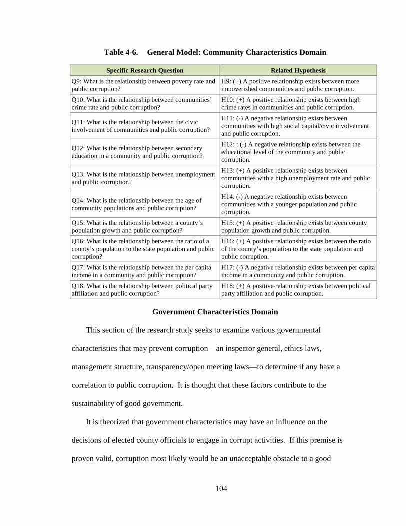
104

Table 4-6. General Model: Community Characteristics Domain

Specific Research Question Related Hypothesis Q9: What is the relationship between poverty rate and public corruption?

H9: (+) A positive relationship exists between more impoverished communities and public corruption.

Q10: What is the relationship between communities’ crime rate and public corruption?

H10: (+) A positive relationship exists between high crime rates in communities and public corruption.

Q11: What is the relationship between the civic involvement of communities and public corruption?

H11: (-) A negative relationship exists between communities with high social capital/civic involvement and public corruption.

Q12: What is the relationship between secondary education in a community and public corruption?

H12: : (-) A negative relationship exists between the educational level of the community and public corruption.

Q13: What is the relationship between unemployment and public corruption?

H13: (+) A positive relationship exists between communities with a high unemployment rate and public corruption.

Q14: What is the relationship between the age of community populations and public corruption?

H14. (-) A negative relationship exists between communities with a younger population and public corruption.

Q15: What is the relationship between a county’s population growth and public corruption?

H15: (+) A positive relationship exists between county population growth and public corruption.

Q16: What is the relationship between the ratio of a county’s population to the state population and public corruption?

H16: (+) A positive relationship exists between the ratio of the county’s population to the state population and public corruption.

Q17: What is the relationship between the per capita income in a community and public corruption?

H17: (-) A negative relationship exists between per capita income in a community and public corruption.

Q18: What is the relationship between political party affiliation and public corruption?

H18: (+) A positive relationship exists between political party affiliation and public corruption.

Government Characteristics Domain

This section of the research study seeks to examine various governmental

characteristics that may prevent corruption—an inspector general, ethics laws,

management structure, transparency/open meeting laws—to determine if any have a

correlation to public corruption. It is thought that these factors contribute to the

sustainability of good government.

It is theorized that government characteristics may have an influence on the

decisions of elected county officials to engage in corrupt activities. If this premise is

proven valid, corruption most likely would be an unacceptable obstacle to a good

105

government, one which citizens believe in and trust. Philp (1987) describes “a just

society which preserves the liberty and security of each citizen,” a society in which

citizens “under a wise system of laws and institutions, good customs and proper mores…

are capable of identifying their own good and the common good.” (p. 7). Banfield (1958)

says, “Corruption on the other hand can lead to a breakdown in shared concerns and

results in factional pursuit of special interests and a reliance on coercion over consensus.

In these situations, coercion indicates a corrupt or corrupted state, perverted and rotten,

where every person is on guard against everyone else in a society of amoral familism” (p.

9).

It is through government that officials exercise influence over decisions, and often

they are able to operate with a high degree of discretion. Governments sometimes

provide an environment wherein officials are able to conceal their behavior and use

power and authority for self-benefit. Elected officials face great temptations in a corrupt

government environment, and enormous pressure to bend to special interests can

supersede good judgment (Caiden 1988).

To explore the role of government characteristics, this study will use five factors

thought to measure this domain: (1) ethics laws, (2) management structure, (3) an

inspector general’s office, (4) transparency and open meeting laws, and (5) employment

growth in the county. These five factors will measure the nature of government in local

communities.

106

Ethics Laws

Research Question 19: What is the relationship between ethics laws and public

corruption?

Hypothesis 19: The more stringent the ethics laws, the less likely public

corruption is to occur.

It is theorized that a negative correlation exists between ethics laws (measured as

highly effective or less effective ethics laws, based on penalties for violations) and public

corruption. The primary purpose of ethics legislation is the reduction of the influence of

money, special interests, and private-sector businesses on public officials. Over the

years, studies have confirmed a possible link between the effectiveness of stringent ethics

laws and the discouragement of unethical behavior by elected officials, but there is little

research to link ethical decision-making by county officials to public corruption (Caiden

1988; Tanzi 1998). This study seeks to add to that body of knowledge and determine if

ethic laws can influence an official’s decision to engage in unethical behavior.

Ethics measures are generally popular with constituents, particularly if the laws are

effective in cleaning up government and reducing the influence of special interests

(Mayer 2001). The literature review supported the notion that ethics laws are effective

and can reduce corruption within government. The literature also suggested that public

support for ethics laws, or any good-government legislation, comes mainly from wealthy

and urban constituents (McFarland 1984; Skowronek 1982).

However, there are some contradictions on the effectiveness of ethic laws in

reducing public corruption. According to Menzel and Benton (1991), “There is scant

evidence to suggest that the adoption of ethics codes by city and counties or even by

107

professional associations has made any real difference in the number of ethical

transgressions committed by appointed and elected officials” (p. 419). This contradiction

is the justification for the study review.

Management Structure of Government

Research Question 20: What is the relationship between the management

structure of government and public corruption?

Hypothesis 20: Under a county manager form of government, there is less public

corruption.

It is posited that a negative correlation exists between government structures

(measured as the percentage of corruption cases identified under a county manager form

of government) and public corruption. In the past, various structural reforms in

American politics have been viewed as influencing public corruption; some were even

thought to deter corruption. Wilson (1966) suggests that a fragmented political system,

with no central manager, opens doors for politicians and others to manipulate government

for their own gain and is a stimulus to corruption. Meier et al. (1992) found “fragmented

political systems make public officials less visible and thus reduce the perceived

probability that corrupt actions will be discovered” (p. 143). However, it is thought that

political systems under a county manager form of government can result in fewer

opportunities for public corruption. Under this type of system, the county manager

controls expenditures, budget, contracts, and staff, while elected officials make policy.

The National Association of Counties identifies four active structures of government

used today: (a) Commission-Administrator (county manager), (b) Commission,

(c) Commission-County Executive, and (d) parishes and consolidated governments. The

108

various forms of government employed by the study sample were included in the

research study to determine if a correlation exists between a particular form of county

government and public corruption.

Under a county manager form of government, the administrative staff oversees

management, day-to-day operations, and the implementation of policies, contracts, and

services as directed by the elected board. It is believed that under this system of

government, there is less opportunity for public corruption among elected officials

(Wilson 1966). Rose-Ackerman (1999) writes that “legislatures frequently delegate

implementation to the executive; I have already argued that this is a desirable way to

limit political corruption” (p. 146).

Office of Inspector General

Research Question 21: What is the relationship between county governments that

employ an inspector general to monitor the ethical behavior of officials and

public corruption?

Hypothesis 21: County governments with an inspector general have fewer

opportunities for public corruption.

It is posited that a negative correlation exists between having an inspector general

(measured as county governments with an Office of the Inspector General) and public

corruption. Corruption can destroy a government system and damage the public’s trust.

According to Ketti (2006), “it may be impossible to eliminate corruption in the United

States. Regulations against corrupt practices and legislation to increase government

transparency have reduced corruption by examining government closely to weed out

waste, fraud, and abuse.”

109

However, it is thought that using an inspector general as a method of reducing

corruption can benefit local governments, since the primary goal of an inspector general

is to restore public trust in government by enforcing honesty and integrity in business

practices. Research suggests that Congress enacted the Inspector General’s Act in the

late 1970s to help restore public trust and eliminate government waste. No supporting

empirical studies have been found that determine what significance an inspector general’s

office may play in reducing corruption in county government, but creation of such an

office could reduce the level of public corruption in large urban counties. It is theorized

that an inspector general will reduce corruption and restore public trust.

Open Meeting Laws / Transparency

Research Question 22: What is the relationship between county governments with

open meeting law provisions and public corruption?

Hypothesis 22: County governments with strict open meeting laws provide

transparency and are less likely to result in public corruption.

It is hypothesized that a negative correlation exists between open meeting laws

(measured as the level of transparency within the county government) and public

corruption. Integrity in governance can largely be associated with a great degree of

transparency (Menzel 2005). Governments whose policies stress openness, and which

value open meeting laws, are less likely to encounter public corruption among elected

officials. Conversely, governments and elected officials that are less concerned about

providing open government and conducting business transparently can create an

environment prone to corruption. Tanzi (1998) suggests, “The lack of transparency in

rules, laws, and processes creates a fertile ground for corruption. Rules are often

110

confusing; the documents specifying them are not publicly available; and, at times, the

rules are changed without properly publicized announcements” (p. 575).

It is thought that an environment supporting open meeting law provisions can

provide positive opportunities for elected officials and the political decision-making

process. An open government creates an environment for citizens to become more

involved, closer to their government and its officials, so it reduces corrupt activities

(Maxwell and Winters 2004). It is believed that transparency within a government’s

management structure allows citizens the opportunity to observe the decisions of elected

officials. Support of an open government from public officials suggests that their

decisions, behavior, and transactions are open to review by citizens, the media, and

watchdog groups. The integrity of governance can be associated with its degree of

transparency (Menzel 2005).

Employment Growth

Research Question 23: What is the relationship between county government

employment growth and public corruption?

Hypothesis 23: The greater the employment growth of county government, the

more likely public corruption is to exist in county government.

It is postulated that a positive correlation exists between employment growth in

county government (measured as a one-year change in employment growth) and public

corruption. An increase in the number of employees indicates an increase in government

revenue and a high rate of activity, both of which offer more opportunities for

disbursement of funds and may, therefore, increase the rate of corruption. Presumably, a

healthier financial environment and positive economic conditions for county government

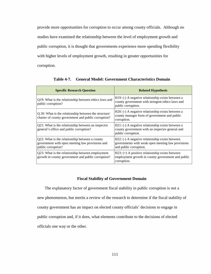
111

provide more opportunities for corruption to occur among county officials. Although no

studies have examined the relationship between the level of employment growth and

public corruption, it is thought that governments experience more spending flexibility

with higher levels of employment growth, resulting in greater opportunities for

corruption.

Table 4-7. General Model: Government Characteristics Domain


Q19: What is the relationship between ethics laws and public corruption?

H19: (-) A negative relationship exists between a county government with stringent ethics laws and public corruption.

Q 20: What is the relationship between the structure/ charter of county government and public corruption?

H20: (-) A negative relationship exists between a county manager form of government and public corruption.

Q21: What is the relationship between an inspector general’s office and public corruption?

H21: (-) A negative relationship exists between a county government with an inspector general and public corruption.

Q22: What is the relationship between a county government with open meeting law provisions and public corruption?

H22: (-) A negative relationship exists between governments with weak open meeting law provisions and public corruption.

Q23: What is the relationship between employment growth in county government and public corruption?

H23: (+) A positive relationship exists between employment growth in county government and public corruption.

Fiscal Stability of Government Domain

The explanatory factor of government fiscal stability in public corruption is not a

new phenomenon, but merits a review of the research to determine if the fiscal stability of

county government has an impact on elected county officials’ decisions to engage in

public corruption and, if it does, what elements contribute to the decisions of elected

officials one way or the other.

112

Early on, scholars began to recognize that corruption has enormous economic and

political consequences on government, creating economic inefficiencies.10

Researchers have suggested that government audits, oversight procedures and

committees, and effective financial policies can deter corruption (Wilson 1966; Walsh

1978; Rose-Ackerman 1978; Fuchs 1986; Klitgaard 1988). This study proposes to

examine the effect that county government financial stability and financial policies have

on public corruption.

The literature

suggests a correlation between the level of economic prosperity and corruption: “As a

country grows richer the level of corruption decreases” (Amundsen 1999, p. 15).

Determining the impact of fiscal stability on local governments and public corruption

thus becomes pertinent to explaining the presence of corruption within local county

governments. For instance, one can plausibly argue that the fiscal stability of

government has the potential to reduce opportunities for corruption; the effectiveness of

fiscal policies, stringent government oversight and regulations, and revenue growth are

all positive factors that benefit governments and reduce the temptations of public

corruption.

To understand the influence of government financial stability on public corruption,

three attributes were proposed for inclusion in this study: (1) financial stability,

(2) federal and state aid, and (3) audit capacity. These factors provided an opportunity to

measure key components of the fiscal characteristics of county government and were

used to develop research questions and hypotheses. The following subsections present

10 Early works that recognized the adverse political and economic consequences of corruption include

Rose-Ackerman (1978 and 1999), Huntington (1968), and Heidenheimer et al. (1989).

113

the specific research questions and related hypotheses for the domain of government

fiscal characteristics.

Financial Stability

Research Question 24: What is the relationship between the financial stability of

county government and public corruption?

Hypothesis 24: The greater the financial stability of county government, the more

likely public corruption is to occur.

It is thought that a positive correlation exists between the financial stability of county

government (measured as the county’s bond rating and annual expenditures) and public

corruption. The bond rating (Exhibit II) of a county government indicates its financial

stability: the higher the rating is, the more financially stable the county is and the more

likely it is that funds are available. It is believed that in financially healthier counties,

more funds are available to finance and fund capital projects, creating more chances for

public corruption to occur. It is also thought that fiscal stability in government represents

security, confidence, and consistent productivity. Bond rating is a good indicator of

fiscal stability.

The literature review showed that many scholars have concluded that when large

sums of money are available for funding projects, including special projects, then access

to government funds opens the door to temptation for corruption (Berg et al. 1976;

Wilson 1966; Maxwell 2004). Goel and Nelson (1998) believed that public spending by

a local government with an excessive availability of funds and little oversight is an

indicator for political rent-seeking and, hence, corruption; more available funds produce

more opportunities for corruption. This study examines these conclusions.

114

Conversely, other researchers believe that a decrease in expenditures can lower

opportunities for disbursing funds, but still open the door to public corruption (Tanzi

1998). Fewer funds bring about more competition for grants and contracts, and people

are willing to pay bribes to receive a share of the limited contracts available. However,

this study theorizes that sound financial policies and procedures can be a preventative

measure for illicit behavior by politicians and bureaucrats. It is hypothesized that “for the

governmental policies to be effective, however, the bureaucracies must actually

implement them. Hence it becomes crucial that officials not be influenced, through graft,

to deviate from their appointed task” (Leff 1964).

Ackerman (1999) suggested that economic distress and unexpected population

growth could increase the demand for government services, create situations of instability

within a government, and lead to opportunities for corruption. It is evident that the factor

of financial stability produces two lines of opinion: more funds available can open the

door to corruption, but a lack of dollars can also provide opportunities for corruption.

Federal and State Aid

Research Question 25: What is the relationship between federal and state aid and

public corruption?

Hypothesis 25: Counties receiving greater federal and state aid are more likely to

experience public corruption.

It is hypothesized that a positive correlation exists between federal and state aid

(measured as the amount of federal and state aid provided to the county during the year of

conviction and as the amount of federal and state aid in proportion to the total

expenditures of the county) and public corruption.

115

Federal law enforcement agencies monitor local governments’ activities when

substantial sums of aid are appropriated from the federal government. It is thought that

high levels of federal and state aid may result in public corruption because they afford

county officials more flexibility in the spending of tax dollars, often with little direct

oversight. Federal officials usually conduct audits long after grants have been awarded

and projects closed out. These opportunities encourage county officials to grant contracts

and allocate dollars to friends and political supporters, increasing the opportunity for

personal gain. Researchers have also suggested that the size of a government budget may

be related to the level of corruption (La Palombara 1994). As noted above, Goel and

Nelson (1998) believed that public spending of local government is an indicator for rent-

seeking activities and corruption.

Auditors

Research Question 26: What is the relationship between the audit capacity of

county government and public corruption?

Hypothesis 26: Counties with an independent internal auditing capacity are less

likely to experience public corruption.

It is theorized that a negative correlation exists between independent auditing

(measured as independent government audits) and public corruption. Independent audits

are a valuable tool in fighting public corruption; they can provide checks and balances in

government to ensure that expenditures of public funds are appropriate and proper.

Audits provide greater assurance that corruption can be limited, and can even deter its

spread; matched with prudent financial policies and procedures, audits can be a powerful

preventative measure against illicit political behavior. Rose-Ackerman (1999) states, “In

116

a government with strong checks and balances, no public institution is all-powerful” (p.

144). The monitoring and enforcement functions of an independent audit can serve as

effective anticorruption strategies and useful tools in the oversight of government budgets

and expenditures, ensuring that government funds are properly appropriated and used for

government projects.

Independent audit functions are more effective in the county manager form of

government, where they are not under the control of elected officials. An autonomous

independent auditor can remove political influence and the pressures that can be created

if the function is managed by elected county officials. To ensure the effectiveness of an

independent audit function, audits and financial reports should be published and made

available for public review. Openness and accountability are positive measures for

elected officials and provide the public with a level of confidence and trust.

The literature review showed that “a great use of audits to enable legislatures to deter

corruption is advocated by many researchers” (Wilson 1966, p. 31; Walsh 1978; Rose-

Ackerman 1978, p. 216; Fuchs 1986, p. 113; and Klitgaard 1988, p. 53). It is thought that

audits will likely detect corrupt actions and can therefore deter corruption (Gardiner and

Lyman 1990).

Prudent fiscal policies established under audit guidelines are positive alternatives to

protect the expenditures of government funds and possibly reduce corruption

opportunities. This study reviews the impact of independent audits to determine if

prudent fiscal management through independent auditors has a relationship to public

corruption.

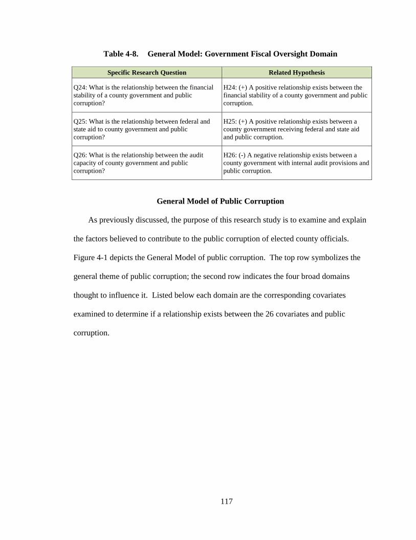
117

Table 4-8. General Model: Government Fiscal Oversight Domain


Q24: What is the relationship between the financial stability of a county government and public corruption?

H24: (+) A positive relationship exists between the financial stability of a county government and public corruption.

Q25: What is the relationship between federal and state aid to county government and public corruption?

H25: (+) A positive relationship exists between a county government receiving federal and state aid and public corruption.

Q26: What is the relationship between the audit capacity of county government and public corruption?

H26: (-) A negative relationship exists between a county government with internal audit provisions and public corruption.

General Model of Public Corruption

As previously discussed, the purpose of this research study is to examine and explain

the factors believed to contribute to the public corruption of elected county officials.

Figure 4-1 depicts the General Model of public corruption. The top row symbolizes the

general theme of public corruption; the second row indicates the four broad domains

thought to influence it. Listed below each domain are the corresponding covariates

examined to determine if a relationship exists between the 26 covariates and public

corruption.

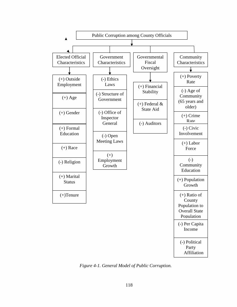
118

Figure 4-1. General Model of Public Corruption.

Public Corruption among County Officials

Elected Official Characteristics


Governmental Fiscal

Oversight


(+) Outside Employment

(-) Ethics Laws (+) Financial

Stability

(+) Poverty Rate

(+) Age

(+) Gender

(+) Formal Education

(+) Race

(-) Religion

(+) Marital Status

(+)Tenure

(-) Structure of Government

(-) Office of Inspector General

(-) Open Meeting Laws

(+) Federal & State Aid

(-) Auditors

(-) Age of Community

(65 years and older)

(+) Crime Rate

(-) Civic Involvement

(+) Labor Force

(-) Community Education

(+) Population

Growth

(+) Ratio of County

Population to Overall State Population

(+) Employment

Growth

(-) Per Capita Income

(-) Political Party

Affiliation

119

CHAPTER 5

FINDINGS OF THE STUDY

County-Level Characteristics

This chapter of the research study presents the analyses, findings, and testing of the

hypotheses for the General Models for both county-level and individual-level

characteristics. As explained in Chapter 1, there were four purposes of this research

study:

1. To explain what variables are likely to predict public corruption among elected

county officials.

2. To examine the predictive variables in which two groups of county officials took

divergent roads in their political career, one group opting to engage in corrupt

behavior and the other opting not to engage in corrupt behavior.

3. To provide a plausible model that could explain the behavior of elected county

officials who chose to engage in public corruption.

4. To identify the characteristics that influence public corruption.

The initial process used in developing the General Models for this study included an

outline of characteristics thought to be predictors or factors that influence the behavior of

county officials and result in the negative behavior of public corruption. As previously

discussed, the dependent variable is a dichotomous variable, indicating whether an

elected official did or did not commit public corruption. The independent variables

related to county-level data included 18 covariates for three domains: government

characteristics, financial characteristics, and community characteristics (Chapter 4

discusses these covariates in detail). Data for these variables were gathered from

counties with populations of 300,000 or more.

120

These 18 variables are thought to influence the behavior of elected officials.

Throughout the research effort, it was theorized that GST was a factor influencing an

elected official's behavior. Including all variables within the domains allowed a broad

explanatory power for the General Model and enhanced the outcome of this study.

Appendix V provides a detailed list of negative strains that influence behavior. GST was

incorporated when interpreting the results of the analysis and is a contributing factor that

influences behavior.

The original data set included two data set categories, county level and individual

level, and incorporated a two-step process that involved county-level data and individual-

level data. The county-level data set consisted of 173 counties over 10 years, though the

final analysis only incorporated 117 counties; as previously stated, 56 counties did not

respond to the request for information.

The individual-level data set consisted of 180 elected officials within 26 counties

over a 10-year span. The analysis for the individual-level data set incorporated only 155

individuals; 25 individuals were excluded from the study because they could not be

located or were deceased.

General Model: Corruption and County-Level Characteristics

The dependent variable is a dichotomous measure coded “1” for committing

corruption and “0” for not committing corruption. There are 18 independent variables for

county-level predictors. The variables for government characteristics were an inspector

general’s office, ethics laws, structure of government, open meeting laws, and

employment growth. The variables for county financial characteristics were per capita

income, financial stability, federal and state aid, and outside auditors. The variables for

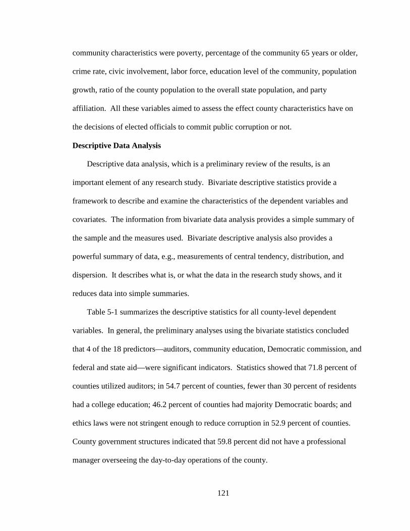
121

community characteristics were poverty, percentage of the community 65 years or older,

crime rate, civic involvement, labor force, education level of the community, population

growth, ratio of the county population to the overall state population, and party

affiliation. All these variables aimed to assess the effect county characteristics have on

the decisions of elected officials to commit public corruption or not.

Descriptive Data Analysis

Descriptive data analysis, which is a preliminary review of the results, is an

important element of any research study. Bivariate descriptive statistics provide a

framework to describe and examine the characteristics of the dependent variables and

covariates. The information from bivariate data analysis provides a simple summary of

the sample and the measures used. Bivariate descriptive analysis also provides a

powerful summary of data, e.g., measurements of central tendency, distribution, and

dispersion. It describes what is, or what the data in the research study shows, and it

reduces data into simple summaries.

Table 5-1 summarizes the descriptive statistics for all county-level dependent

variables. In general, the preliminary analyses using the bivariate statistics concluded

that 4 of the 18 predictors—auditors, community education, Democratic commission, and

federal and state aid—were significant indicators. Statistics showed that 71.8 percent of

counties utilized auditors; in 54.7 percent of counties, fewer than 30 percent of residents

had a college education; 46.2 percent of counties had majority Democratic boards; and

ethics laws were not stringent enough to reduce corruption in 52.9 percent of counties.

County government structures indicated that 59.8 percent did not have a professional

manager overseeing the day-to-day operations of the county.

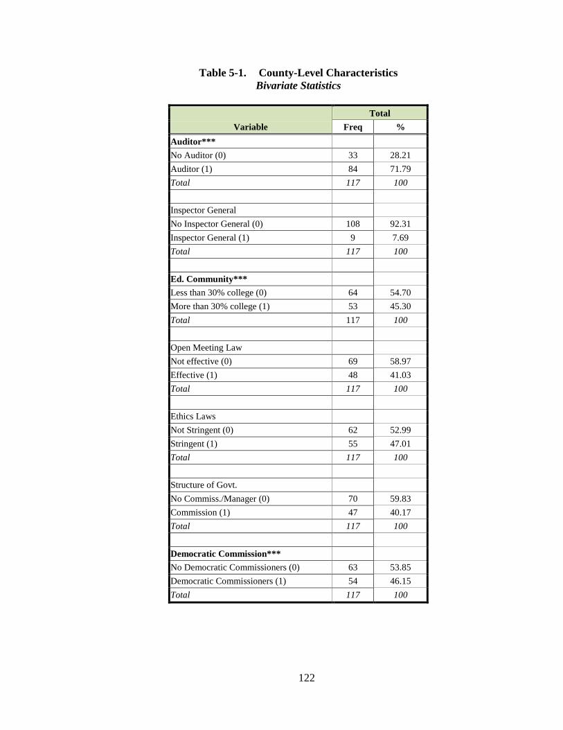
122

Table 5-1. County-Level Characteristics Bivariate Statistics

Variable Total

Freq % Auditor*** No Auditor (0) 33 28.21 Auditor (1) 84 71.79 Total 117 100 Inspector General No Inspector General (0) 108 92.31 Inspector General (1) 9 7.69 Total 117 100 Ed. Community*** Less than 30% college (0) 64 54.70 More than 30% college (1) 53 45.30 Total 117 100 Open Meeting Law Not effective (0) 69 58.97 Effective (1) 48 41.03 Total 117 100 Ethics Laws Not Stringent (0) 62 52.99 Stringent (1) 55 47.01 Total 117 100 Structure of Govt. No Commiss./Manager (0) 70 59.83 Commission (1) 47 40.17 Total 117 100 Democratic Commission*** No Democratic Commissioners (0) 63 53.85 Democratic Commissioners (1) 54 46.15 Total 117 100

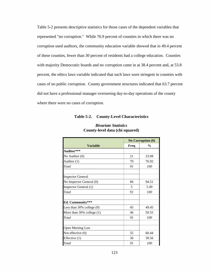
123

Table 5-2 presents descriptive statistics for those cases of the dependent variables that

represented "no corruption." While 76.9 percent of counties in which there was no

corruption used auditors, the community education variable showed that in 49.4 percent

of these counties, fewer than 30 percent of residents had a college education. Counties

with majority Democratic boards and no corruption came in at 38.4 percent and, at 53.8

percent, the ethics laws variable indicated that such laws were stringent in counties with

cases of no public corruption. County government structures indicated that 63.7 percent

did not have a professional manager overseeing day-to-day operations of the county

where there were no cases of corruption.

Table 5-2. County-Level Characteristics

Bivariate Statistics County-level data (chi squared)

Variable No Corruption (0) Freq %

Auditor*** No Auditor (0) 21 23.08 Auditor (1) 70 76.92 Total 91 100 Inspector General No Inspector General (0) 86 94.51 Inspector General (1) 5 5.49 Total 91 100 Ed. Community*** Less than 30% college (0) 45 49.45 More than 30% college (1) 46 50.55 Total 91 100 Open Meeting Law Not effective (0) 55 60.44 Effective (1) 36 39.56 Total 91 100

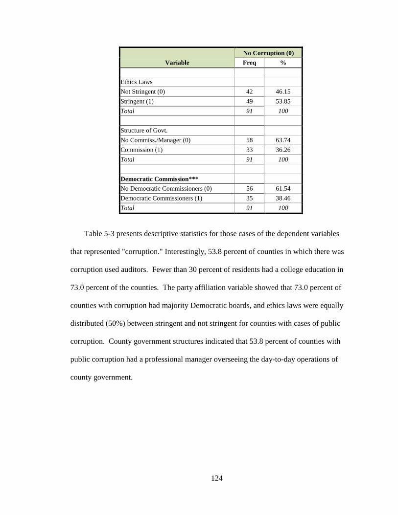
124

Variable No Corruption (0) Freq %

Ethics Laws Not Stringent (0) 42 46.15 Stringent (1) 49 53.85 Total 91 100 Structure of Govt. No Commiss./Manager (0) 58 63.74 Commission (1) 33 36.26 Total 91 100 Democratic Commission*** No Democratic Commissioners (0) 56 61.54 Democratic Commissioners (1) 35 38.46 Total 91 100

Table 5-3 presents descriptive statistics for those cases of the dependent variables

that represented "corruption." Interestingly, 53.8 percent of counties in which there was

corruption used auditors. Fewer than 30 percent of residents had a college education in

73.0 percent of the counties. The party affiliation variable showed that 73.0 percent of

counties with corruption had majority Democratic boards, and ethics laws were equally

distributed (50%) between stringent and not stringent for counties with cases of public

corruption. County government structures indicated that 53.8 percent of counties with

public corruption had a professional manager overseeing the day-to-day operations of

county government.

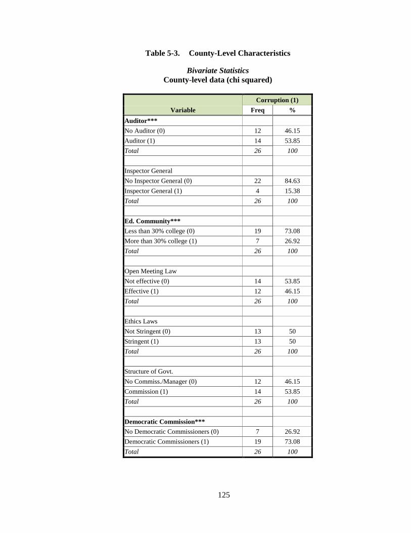
125

Table 5-3. County-Level Characteristics

Bivariate Statistics County-level data (chi squared)

Variable Corruption (1)

Freq % Auditor*** No Auditor (0) 12 46.15 Auditor (1) 14 53.85 Total 26 100 Inspector General No Inspector General (0) 22 84.63 Inspector General (1) 4 15.38 Total 26 100 Ed. Community*** Less than 30% college (0) 19 73.08 More than 30% college (1) 7 26.92 Total 26 100 Open Meeting Law Not effective (0) 14 53.85 Effective (1) 12 46.15 Total 26 100 Ethics Laws Not Stringent (0) 13 50 Stringent (1) 13 50 Total 26 100 Structure of Govt. No Commiss./Manager (0) 12 46.15 Commission (1) 14 53.85 Total 26 100 Democratic Commission*** No Democratic Commissioners (0) 7 26.92 Democratic Commissioners (1) 19 73.08 Total 26 100

126

Table 5-4 summarizes the descriptive statistics for the remaining covariates in the

county-level characteristics category of the General Model. The variables are listed in

order by domain: county government characteristics, government fiscal performance

characteristics, and community characteristics.

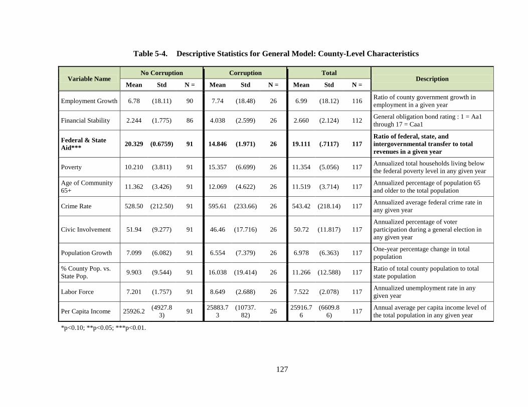
127

Table 5-4. Descriptive Statistics for General Model: County-Level Characteristics

Variable Name No Corruption Corruption Total

Description Mean Std N = Mean Std N = Mean Std N =

Employment Growth 6.78 (18.11) 90 7.74 (18.48) 26 6.99 (18.12) 116 Ratio of county government growth in employment in a given year

Financial Stability 2.244 (1.775) 86 4.038 (2.599) 26 2.660 (2.124) 112 General obligation bond rating : 1 = Aa1 through 17 = Caa1

Federal & State Aid*** 20.329 (0.6759) 91 14.846 (1.971) 26 19.111 (.7117) 117

Ratio of federal, state, and intergovernmental transfer to total revenues in a given year

Poverty 10.210 (3.811) 91 15.357 (6.699) 26 11.354 (5.056) 117 Annualized total households living below the federal poverty level in any given year

Age of Community 65+ 11.362 (3.426) 91 12.069 (4.622) 26 11.519 (3.714) 117 Annualized percentage of population 65

and older to the total population

Crime Rate 528.50 (212.50) 91 595.61 (233.66) 26 543.42 (218.14) 117 Annualized average federal crime rate in any given year

Civic Involvement 51.94 (9.277) 91 46.46 (17.716) 26 50.72 (11.817) 117 Annualized percentage of voter participation during a general election in any given year

Population Growth 7.099 (6.082) 91 6.554 (7.379) 26 6.978 (6.363) 117 One-year percentage change in total population

% County Pop. vs. State Pop. 9.903 (9.544) 91 16.038 (19.414) 26 11.266 (12.588) 117 Ratio of total county population to total

state population

Labor Force 7.201 (1.757) 91 8.649 (2.688) 26 7.522 (2.078) 117 Annualized unemployment rate in any given year

Per Capita Income 25926.2 (4927.83) 91 25883.7

3 (10737.

82) 26 25916.76

(6609.86) 117 Annual average per capita income level of

the total population in any given year

*p<0.10; **p<0.05; ***p<0.01.

128

Logit Regression Analysis - Corruption and County-Level Characteristics

The objective of this research is to identify county-level characteristics likely to

predict the maximum probability of elected county officials committing public

corruption. A logit regression analysis will assist in identifying the predictors and can

determine if any of the variables are related to negative strains that may also influence the

behavior of public officials. The analysis will identify variables that may be related to

GST and provide a theoretical explanation of county-level characteristics likely to

influence elected officials' decisions to commit acts of criminal public corruption.

The General Model category for county-level data included 18 independent variables

used to predict the potential for public corruption. Table 5-5 presents the results of the

logit analysis for the general model. The results of the analysis suggest that the

likelihood ratio chi-square of 66.27 tells us the model as a whole fits and that the

inclusion of the independent variable significantly improved the model’s explanatory

power. A review of the coefficients provide support for the role of five variables

(Auditor, Per Capita Income, Financial Stability, Poverty and County Population) in

explaining the likelihood of county government experiencing corruption. Two other

variables, Inspector General and Community Education, had coefficients in the

hypothesized direction but fell short of statistical significance. The remaining eleven

variable were neither significant nor in the predicted direction. The coefficients are

important and the standard measure in conducting a logit analysis. However, it is much

easier to explain the results if coefficient which are the log odds converted into odds ratio

and this has been done in Table 5-5.

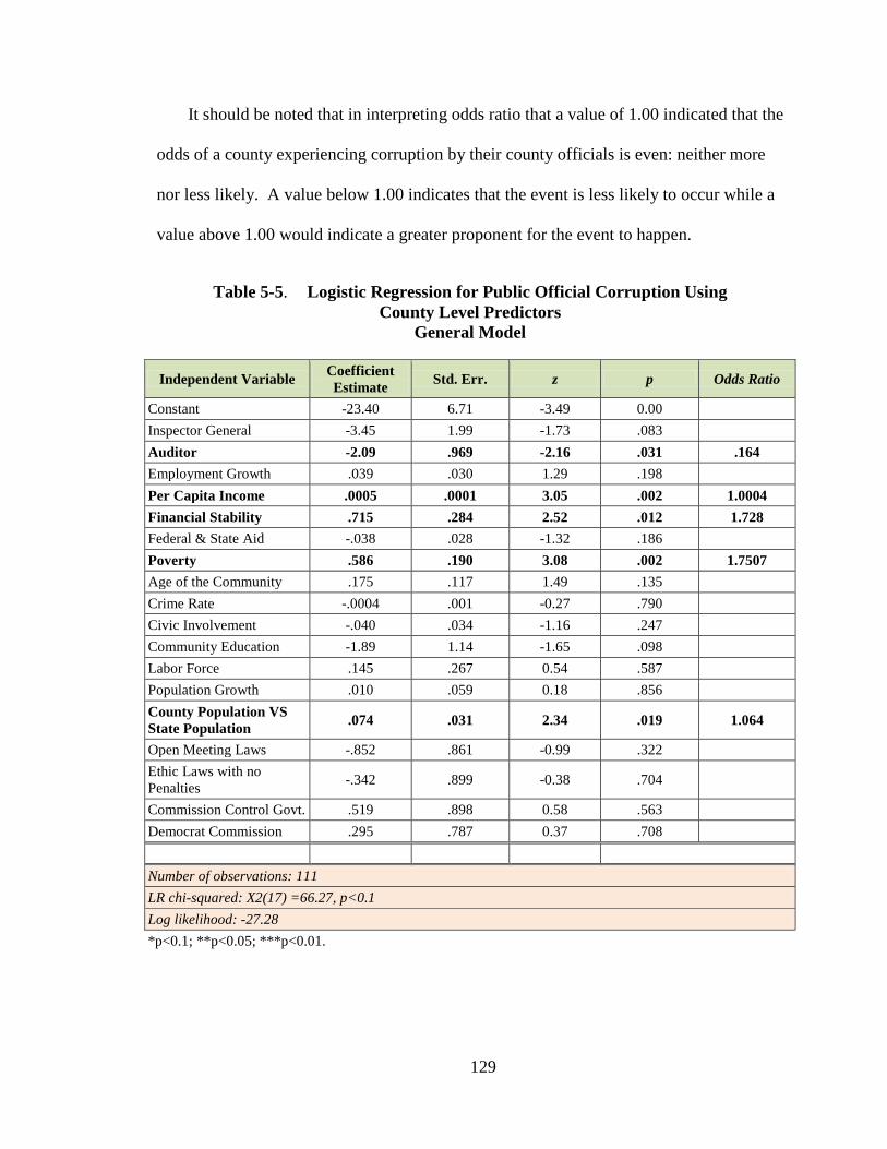
129

It should be noted that in interpreting odds ratio that a value of 1.00 indicated that the

odds of a county experiencing corruption by their county officials is even: neither more

nor less likely. A value below 1.00 indicates that the event is less likely to occur while a

value above 1.00 would indicate a greater proponent for the event to happen.

Table 5-5. Logistic Regression for Public Official Corruption Using County Level Predictors

General Model

Independent Variable Coefficient Estimate Std. Err. z p Odds Ratio

Constant -23.40 6.71 -3.49 0.00 Inspector General -3.45 1.99 -1.73 .083 Auditor -2.09 .969 -2.16 .031 .164 Employment Growth .039 .030 1.29 .198 Per Capita Income .0005 .0001 3.05 .002 1.0004 Financial Stability .715 .284 2.52 .012 1.728 Federal & State Aid -.038 .028 -1.32 .186 Poverty .586 .190 3.08 .002 1.7507 Age of the Community .175 .117 1.49 .135 Crime Rate -.0004 .001 -0.27 .790 Civic Involvement -.040 .034 -1.16 .247 Community Education -1.89 1.14 -1.65 .098 Labor Force .145 .267 0.54 .587 Population Growth .010 .059 0.18 .856 County Population VS State Population .074 .031 2.34 .019 1.064

Open Meeting Laws -.852 .861 -0.99 .322 Ethic Laws with no Penalties -.342 .899 -0.38 .704

Commission Control Govt. .519 .898 0.58 .563 Democrat Commission .295 .787 0.37 .708

Number of observations: 111 LR chi-squared: X2(17) =66.27, p<0.1 Log likelihood: -27.28 *p<0.1; **p<0.05; ***p<0.01.

130

The results indicate that the model's statistically significant variables produced

strong substantive effects: when measured against corruption, these five predictors were

statistically significant. The model fits sufficiently well, based on the results of the log

likelihood test comparing the general model with the null constant only test.

The data for the variable auditor is statistically significant at p-value=.031. The odds

ratio is .1237and suggests that counties with auditors are less likely to experience public

corruption. In fact, one can say that they are 12% less likely to experience corruption

than counties with no auditors. As hypothesized, results indicate that auditors can reduce

public corruption, could be a valuable tool to limit public corruption in government.

The results for the predictor per capita income were statistically significant at p-value

= .002 and suggest that counties with a higher per capita income are slightly more likely

to experience corruption among their public officials. While, the performance of this

variable suggests that counties with lower per capita income are less likely to experience

public corruption than counties with high per capita income, it should be noted that the

odds ratio is very close to 1.0 indicating only a marginal impact. Per capita income

within communities appears to influence the behavior of public officials. It was theorized

that the overall wealth of a community is a indicator of its tolerance for corruption.

Initially it was hypothesized that wealthy communities would be less tolerant of public

corruption; however, the data does not support this. In addition, there was a presumption

with this variable that GST is applicable. With the belief, Agnew (2001) suggests,

“create some pressure or incentive to engage in criminal activities as a coping

mechanism” (p. 320).

However, this was not occurring in the corruption of county elected officials.

131

The predicted probability for financial stability suggests that the greater the financial

stability of county government, the more likely public corruption is to occur. Financial

stability was statistically significant at p-value= .012. This result suggest that counties

with a high bond rating are more likely to have public officials engage in acts of public

corruption because the higher the bond rating, the greater the county's financial strength.

In fact, the odds of corruption occurring is two times more likely for every unit increase

in the bond rating. The results of the analysis are consistent with the stated hypothesis,

which held that public corruption was more likely to occur in counties with greater fiscal

stability. It turned out that higher bond ratings result in lower interest rates to borrow

funds that can be used for capital projects, which can lead to corruption.

The predicted probability for poverty rate suggests that poverty influences the behavior

of public officials. This finding is consistent with the stated hypothesis, in which

impoverished communities are more likely to have public officials who engage in

corruption. The coefficient measuring poverty is statistically significant at p-value= .002.

The odd ratio is 1.80 indicates that a one unit increase in poverty will increase the

likelihood of corruption by 80%. The poverty variable is indicative of negative strains,

and the probability exists of a relationship between poverty and GST. This value

increases because as poverty grows, corruption tends to increase. Communities with a

high rate of poverty would suggest a high rate of corruption. Interesting there seems to

be a contradiction in the results. But the per capita income variable indicates that higher

per capita income results in slightly more corruption. It might be that large cities do

indeed have two economic factors at play. High poverty might create an environment

132

where corruption is tolerated and there are opportunities because communities have the

resources to spend on government. Those resources create an opportunity for corruption.

Finally, the predicted probability for percent of county population compared to state

population is statistically significant at p-value = .019. The finding shows that serving in

counties whose population is a majority of the state’s population can influence the

behavior of public officials. The results suggest that as the population of such counties

increases, corruption is likely to increase as well. In fact, public officials serving in

counties with a larger percentage of the state population are more likely to be corrupt.

The results suggest that for every one unit change in the county population compared to

the state population there is an 8% change in the probability of public corruption.

Conversely, the results also suggest that public officials in counties with a lower

percentage of the state’s population are less likely to engage in acts of corruption.

In sum, a majority of the hypothesis were not significant. However, five variables

were significant and were found to increase our understanding of when corruption might

occur in county government.

Chapter 6 presents final comments and conclusions regarding the General Model

analyses.

Individual-Level Characteristics

General Model: Corruption and Individual-Level Characteristics

Thus far the analysis has focused on explaining the characteristics of the counties

where corrupted has occurred. It should be obvious that even through some counties are

more likely to experience corruption; it is highly unlikely that in every one of those

counties all of the elected officials were guilty of participating in corruption. The

133

research now turns to understanding if there are some characteristics of elected officials

that might make them more likely to engage in corruption than other officials. The data

for this research are all those officials elected in a county where at least one county

official was found to commit a corrupt act as we have defined corruption. The dependent

variable in this phase of analysis was a dichotomous measure coded "1" for any elected

official found to engage in corruption and "0" for those not involved. The information

presented includes the eight predictors used in assessing which profile characteristics are

likely to result in elected officials committing public corruption or not. The independent

variables for individual-level predictors were gender, marital status, age race, education,

religious belief, tenure and outside employment. Age was broken out into a series of

dummy variables

Descriptive Data Analysis

The initial analysis proceeds in two phases. First, six of the eight variables lend

themselves to analysis using simple 2x2 categorical analyses and that analysis is provided

in Table 5-6. Two other variables, level of formal education and tenure in office are

continuous data and the analysis is presented in Table 5-7 as difference of means. Table

5-6 provides the bivariate analysis of six variables with the dependent variable

corruption. Some very interesting results appear in the table. Three of the four dummy

variables for age were relatively similar with anywhere from 20% to 28% of the age

group participating in corruption. However, elected officials in the 50 to 59--age range

were more likely to participate in some corruption. It would also appear that Race and

Gender variables operated as hypothesized. Non-white were more likely to engage in

corruption than their white counterparts. Males were more likely, by a significant

134

percentage (34% to 16%), to have participated in a corruptible act than females elected

officials. The data in Table 5-6 provides evidence that elected officials who did not see

themselves as religious were more likely to engage in an illegal act 42% of the non-

religious officials compared to only 18% of those categorized as religious. Interestingly

married officials were more prone to engage in illegal acts.

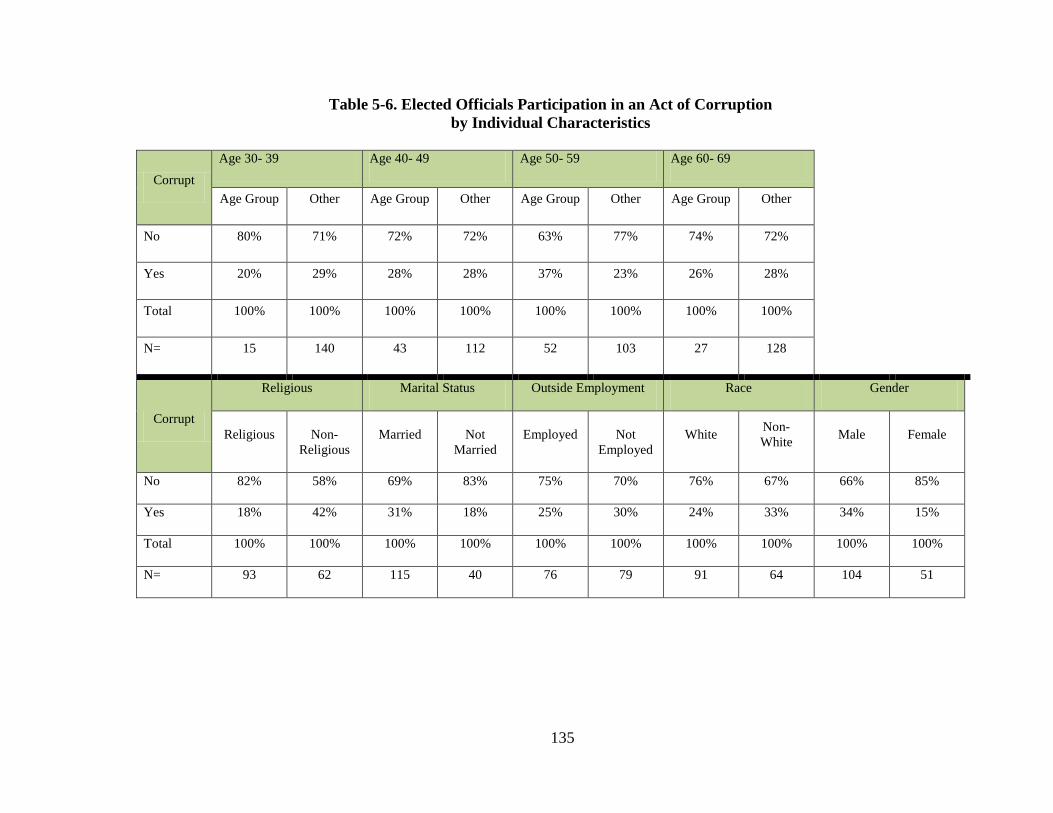
135

Table 5-6. Elected Officials Participation in an Act of Corruption by Individual Characteristics

Corrupt Age 30- 39 Age 40- 49 Age 50- 59 Age 60- 69

Age Group Other Age Group Other Age Group Other Age Group Other

No 80% 71% 72% 72% 63% 77% 74% 72%

Yes 20% 29% 28% 28% 37% 23% 26% 28%

Total 100% 100% 100% 100% 100% 100% 100% 100%

N= 15 140 43 112 52 103 27 128

Corrupt

Religious Marital Status Outside Employment Race Gender

Religious Non-Religious

Married Not Married

Employed

Not Employed

White Non- White Male Female

No 82% 58% 69% 83% 75% 70% 76% 67% 66% 85%

Yes 18% 42% 31% 18% 25% 30% 24% 33% 34% 15%

Total 100% 100% 100% 100% 100% 100% 100% 100% 100% 100%

N= 93 62 115 40 76 79 91 64 104 51

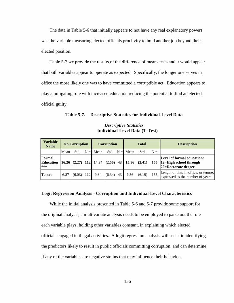
136

The data in Table 5-6 that initially appears to not have any real explanatory powers

was the variable measuring elected officials proclivity to hold another job beyond their

elected position.

Table 5-7 we provide the results of the difference of means tests and it would appear

that both variables appear to operate as expected. Specifically, the longer one serves in

office the more likely one was to have committed a corruptible act. Education appears to

play a mitigating role with increased education reducing the potential to find an elected

official guilty.

Table 5-7. Descriptive Statistics for Individual-Level Data

Descriptive Statistics Individual-Level Data (T-Test)

Variable Name No Corruption Corruption Total Description

Mean Std. N = Mean Std. N = Mean Std. N = Formal Education***

16.26 (2.27) 112 14.84 (2.50) 43 15.86 (2.41) 155 Level of formal education: 12=High school through 20=Doctorate degree

Tenure 6.87 (6.03) 112 9.34 (6.34) 43 7.56 (6.19) 155 Length of time in office, or tenure, expressed as the number of years

Logit Regression Analysis - Corruption and Individual-Level Characteristics

While the initial analysis presented in Table 5-6 and 5-7 provide some support for

the original analysis, a multivariate analysis needs to be employed to parse out the role

each variable plays, holding other variables constant, in explaining which elected

officials engaged in illegal activities. A logit regression analysis will assist in identifying

the predictors likely to result in public officials committing corruption, and can determine

if any of the variables are negative strains that may influence their behavior.

137

Additionally, a review of the results will determine if GST provides a theoretical

explanation of elected officials' decisions to commit acts of criminal public corruption.

The Logit Model category for individual-level data included eight independent

variables used to predict the likelihood an official would engage in public corruption.

Following are the results of the analysis for the model using logit regression analysis.

The general model incorporates the eight covariates in this research study. However, the

variable age has been modified for the analysis in order to more clearly examine the

hypothesis with regard to age. Thus, there are now four dummy variables for four

different age categories. Elected officials over 70 serve the response group. As a result,

the analysis now discusses the results in the context of eleven variables. As explained

previously; logit regression analysis can aid in determining the probability of elected

public officials committing public corruption. The logit model presented in Table 5-8

was statistically significant at the .001 level. This level of chi-square significance

indicates that the general model fit well compared to null constant only model. In fact,

the variables produced strong substantive effects. The logit regression analysis, which

incorporates eleven covariates with six shown to have statistically significant effects on

corruption: (3 of the 4) age, faith, education and tenure.

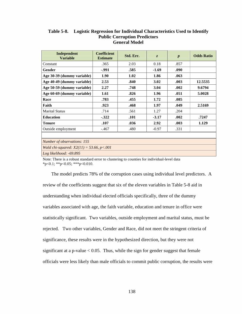
138

Table 5-8. Logistic Regression for Individual Characteristics Used to Identify Public Corruption Predictors

General Model

Independent Variable

Coefficient Estimate Std. Err. z p Odds Ratio

Constant .365 2.03 0.18 .857 Gender -.991 .585 -1.69 .090 Age 30-39 (dummy variable) 1.90 1.02 1.86 .063 Age 40-49 (dummy variable) 2.53 .840 3.02 .003 12.5535 Age 50-59 (dummy variable) 2.27 .748 3.04 .002 9.6794 Age 60-69 (dummy variable) 1.61 .826 1.96 .051 5.0028 Race .783 .455 1.72 .085 Faith .923 .468 1.97 .049 2.5169 Marital Status .714 .561 1.27 .204 Education -.322 .101 -3.17 .002 .7247 Tenure .107 .036 2.92 .003 1.129 Outside employment -.467 .480 -0.97 .331

Number of observations: 155 Wald chi-squared: X2(11) = 53.66, p<.001 Log likelihood: -69.895 Note: There is a robust standard error to clustering to counties for individual-level data *p<0.1; **p<0.05; ***p<0.010. The model predicts 78% of the corruption cases using individual level predictors. A

review of the coefficients suggest that six of the eleven variables in Table 5-8 aid in

understanding when individual elected officials specifically, three of the dummy

variables associated with age, the faith variable, education and tenure in office were

statistically significant. Two variables, outside employment and marital status, must be

rejected. Two other variables, Gender and Race, did not meet the stringent criteria of

significance, these results were in the hypothesized direction, but they were not

significant at a p-value < 0.05. Thus, while the sign for gender suggest that female

officials were less likely than male officials to commit public corruption, the results were

139

not significant. While two studies, Mauro (1993 and LaPorta et al. (1999) found a

relationship between race and public corruption, we were not able to confirm this.

The data for faith (or religious belief) are also consistent with the earlier bivariate

analysis and suggest that public officials who do not demonstrate a religious faith are 2.5

times more likely to commit public corruption than officials who do proclaim some

strong religious belief system (p-value=.049).

The study's intent was to determine is an empirical connection exists between

religion and corruption and it appears to exist. Some researchers link religion to social

environment, including trust and ethics: "Religion provides a language of ethics and,

often an actual 'list of rules to live by'" (Marquette 2010, p.3). Others suggest that public

servants derive their ethical framework in part from their religious beliefs.

The results for the various age predictors compare four different categories of elected

officials to the referent group of elected public officials 70 years and older. Officials who

are 40–49 years of age are 12.5 times more likely to commit an act of corruption than

others (significant at p-value=.003). Public officials who are 50–59 years of age were

slightly less likely to be involved in criminal activities than the 40-49 years of age group,

but were still more than 9 times more likely than the general populations of elected

officials especially are plus 70 age group. This downward trend continued for the next

age category 60-69. This last age group is significant (at the p<.051 level) and more than

5 times more likely to be found guilty that the reference group. All of the evidence

would seem to suggest that as elected officials get older they become less likely to

engage in corruption. These results are contrary to the original hypothesis. It might well

be that younger officials are more likely to engage in acts of corruption as they try to

140

make their mark while older officials are established and financially secure (they may

perhaps even be retired) and do not see the necessity to engage in risky criminal acts.

The information for formal education is supportive of the original hypothesis that the

higher ones education level the lower the probability of engaging in corruption. The odds

ratio is .7247 and indicate that a one unit change in education decrease the probability of

being involved in an act of corruption by 73%. It was theorized that officials with a high

school education or less would feel the pressure to engage in public corruption to

improve their social and economic status. Since education is viewed as a mark of social

status and an indicator of economic achievement, it was believed that a person with a

college degree would not have as much pressure to engage in public corruption. The lack

of education is viewed as a negative strain and should be a negative factor for officials

without a college education, resulting in a greater likelihood of their committing the

crime of public corruption; however, the findings did not support this theory.

These results for tenure suggest that officials who have more years in public office

are slightly more likely to participate in criminal acts than officials with fewer years in

office. The results for the predictor tenure were statistically significant at p-value=.003

and suggest that for a one unit increase in the years of service the odds of committing

public corruption increases by .11%. In sum, the findings for the results for tenure

suggest that it influences the behavior of elected officials and is a predictor of corruption.

Finally, it appears GST influenced only one of the eight predictors chosen to

measure individual profile characteristics of public officials. The results suggest that the

predictor age can influence the decisions of public officials in cases where there are

141

indictments or convictions of public corruption. The predictor age was the only variable

that produced significant results of GST.

Age is also a negative strain it can be viewed in the context of older officials with

failing health, or in the context of young officials who lack social and financial security.

Either would result in negative strain. The determination that one of the individual

variables within the model for individual-level characteristics was a negative strain and

suggest that GST is a factor in the decisions of officials who commit public corruption

when age is a consideration.

Although the results of the eight individual profile characteristics and there

connection to GST did not produce substantial results it does however suggest age is a

possible factor for elected officials who opt to commit illegal acts of corruption.

142

CHAPTER 6

SUMMARY, CONCLUSION AND RECOMMENDATIONS

Discussion and Summary of Results

This research study is intended to add to the body of knowledge about, and improve

our understanding of, public corruption in county government and among elected county

officials. It seeks to explain those factors identified as predictors of public corruption and

develop recommendations to improve further research on the topic. To accomplish this

task, two models were explored and developed: the first General Model, which examined

county-level characteristics, and the second General Model, which examined the profile

characteristics of public officials, along with the influence these characteristics play in

the behavior of county officials who commit public corruption. Consistent with the

theoretical model, it was found that age, religious faith, education, tenure, auditor, per

capita income, financial stability, poverty, and the percentage of county population

compared to state population were all highly relevant to the likelihood of elected officials

engaging in criminal activities.

Secondly, the study sought to determine the influence GST played in the behavior

and decisions of public officials.

General Model: County-Level Characteristics

The General Model of county-level characteristics contained in this study proposed

18 hypotheses within the three domains of interest, and statistical significance was found

for five of the covariates (p-values < 0.05): auditor, per capita income, financial stability,

poverty, and percentage of county population compared to state population. No

statistically significant evidence of a relationship to public corruption was found for the

143

remaining 13 covariates: inspector general, ethics laws, county government structure,

open meeting laws, employment growth, federal and state aid, age of the community,

crime rate, civic involvement, community education, unemployment rate, population

growth, and political party affiliation. However, the results of this study suggest GST

produced a cause-and-effect influence on two covariates: per capita income, and poverty.

First, this research examined the effect the auditor variable has on committing

corruption. The study determined that county governments with audit functions results in

less corruption consistent with the literature. The literature review (Wilson 1966, p. 31;

Walsh 1978; Rose-Ackerman 1978, p. 216; Fuchs 1986, p. 113; Klitgaard 1988, p. 53)

discovered that auditors in government deter public corruption and consequently decrease

its incidence. The research results validate the hypothesis that public corruption can be

reduced when county governments use internal auditors and implement policies to

monitor the spending of public funds. Some governments that want to reduce public

corruption have established internal audit divisions that are independent of elected

officials’ influence. The effectiveness of auditors depends on their ability to remain

independent with no barriers, and their ability to report waste and fraud. The independent

nature of this function can influence the outcome; for example, this study found that

county governments with independent auditors are less likely to experience corruption.

Two possible explanations of the effectiveness of this covariate are (1) the fear of being

caught, and (2) the effectiveness of an independent office free to report fraud and waste.

Second, research results showed the covariate per capita income appears to influence

public corruption. The logit model examined this factor and determined there was a

significant, but small indication that the wealth of a community can determine its

144

tolerance (or lack thereof) for public corruption. The results show that the greater the

wealth of a community, the more likely it is to find corruption. Authors such as

Amundsen (1999) and Maxwell and Winters (2004) suggest that citizens residing in

communities with high per capita incomes, or civic-minded citizens, are more

knowledgeable about the activities of their elected officials and more inclined to monitor

those activities, and as a result, corruption decreases. The results of the study suggest the

opposite; communities with high per capita income, corruption is more likely to exist.

The result of the analysis was inconsistent with the hypothesis.

Third, this research examined the relationship between the financial stability of

county government and the likelihood of officials committing public corruption. The

analysis discovered that a relationship does exist: when county governments have

substantial funding or other financial resources available to award contracts and fund

projects, corruption is more likely to occur. The variable is statistically significant, and

the results suggest a strong relationship; the fiscal performance of counties appears to

influence officials to engage in criminal activity. The results are consistent with the

proposed hypothesis. This factor’s contribution to the likelihood of corruption may be

due to the ability of a county government with an excellent bond rating to generate

financing and funds for capital improvement projects, which in turn makes it possible to

award projects and contracts using government dollars. Previous research that explored

the financial stability of government suggests that governments flush with money are

more likely to experience corruption.

Fourth, the findings in this study show that poverty rate has a direct relationship on

the decision of officials to commit public corruption. This variable provided positive

145

statistical results, indicating that the hypothesis was consistent with the findings. The

results suggest that a high rate of poverty indicates citizens who are preoccupied with

their personal obligations and lack the time to monitor the decisions and behavior of

elected officials. The analysis shows that impoverished communities are the least likely

to monitor the behavior of public officials, and therefore experience a greater degree of

public corruption. The results also suggest that large urban counties with a high rate of

poverty have more incidents of public corruption, and as the poverty rate increases,

corruption is likely to increase. Lastly, the research study suggests that citizens in poor

communities are less likely to demand accountability; they are also generally less

educated, lack the time to monitor the actions of public officials, and lack an

understanding of the mechanics of government.

Lastly, the results of the covariate county population compared to state population

appear to be a positive predictor of public corruption. The logit analysis that examined

this factor found that counties with populations that make up the majority of the state

population provide positive results, which is consistent with the hypothesis. Some

potential explanations are that large urban counties generally experience more crime,

have a high rate of poverty, have the financial resources to fund capital projects, wield

power and influence, and are often the economic engine that supports the state

financially. These counties are also large government institutions with multiple agencies,

and are usually involved in various aspects of government functions and responsibilities.

The counties manage and control various aspects of government. The elected officials

governing these counties wield considerable power and influence, and often control huge

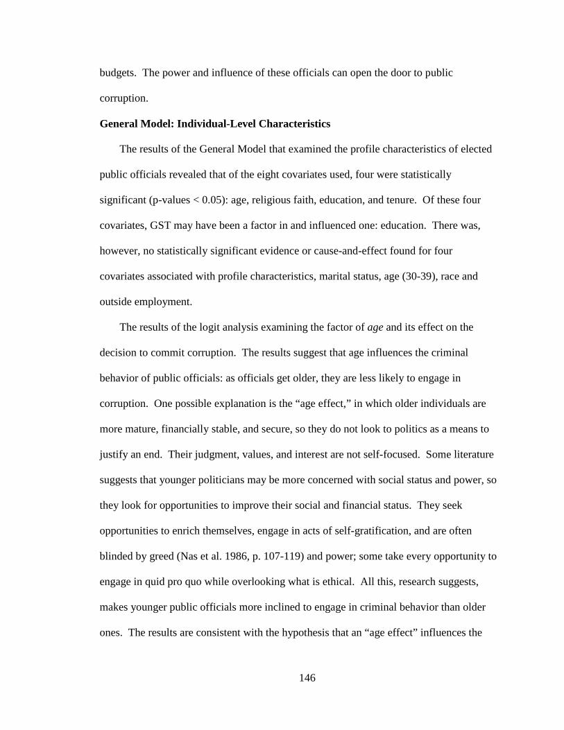
146

budgets. The power and influence of these officials can open the door to public

corruption.

General Model: Individual-Level Characteristics

The results of the General Model that examined the profile characteristics of elected

public officials revealed that of the eight covariates used, four were statistically

significant (p-values < 0.05): age, religious faith, education, and tenure. Of these four

covariates, GST may have been a factor in and influenced one: education. There was,

however, no statistically significant evidence or cause-and-effect found for four

covariates associated with profile characteristics, marital status, age (30-39), race and

outside employment.

The results of the logit analysis examining the factor of age and its effect on the

decision to commit corruption. The results suggest that age influences the criminal

behavior of public officials: as officials get older, they are less likely to engage in

corruption. One possible explanation is the “age effect,” in which older individuals are

more mature, financially stable, and secure, so they do not look to politics as a means to

justify an end. Their judgment, values, and interest are not self-focused. Some literature

suggests that younger politicians may be more concerned with social status and power, so

they look for opportunities to improve their social and financial status. They seek

opportunities to enrich themselves, engage in acts of self-gratification, and are often

blinded by greed (Nas et al. 1986, p. 107-119) and power; some take every opportunity to

engage in quid pro quo while overlooking what is ethical. All this, research suggests,

makes younger public officials more inclined to engage in criminal behavior than older

ones. The results are consistent with the hypothesis that an “age effect” influences the

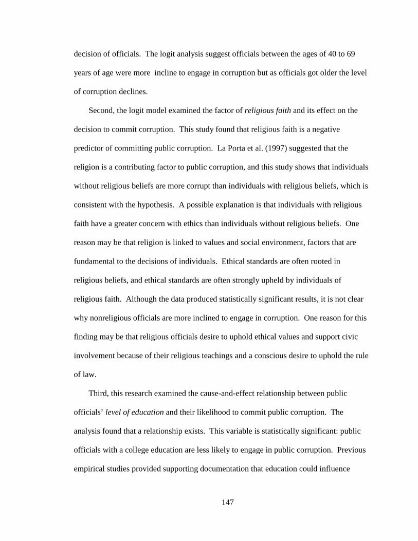
147

decision of officials. The logit analysis suggest officials between the ages of 40 to 69

years of age were more incline to engage in corruption but as officials got older the level

of corruption declines.

Second, the logit model examined the factor of religious faith and its effect on the

decision to commit corruption. This study found that religious faith is a negative

predictor of committing public corruption. La Porta et al. (1997) suggested that the

religion is a contributing factor to public corruption, and this study shows that individuals

without religious beliefs are more corrupt than individuals with religious beliefs, which is

consistent with the hypothesis. A possible explanation is that individuals with religious

faith have a greater concern with ethics than individuals without religious beliefs. One

reason may be that religion is linked to values and social environment, factors that are

fundamental to the decisions of individuals. Ethical standards are often rooted in

religious beliefs, and ethical standards are often strongly upheld by individuals of

religious faith. Although the data produced statistically significant results, it is not clear

why nonreligious officials are more inclined to engage in corruption. One reason for this

finding may be that religious officials desire to uphold ethical values and support civic

involvement because of their religious teachings and a conscious desire to uphold the rule

of law.

Third, this research examined the cause-and-effect relationship between public

officials’ level of education and their likelihood to commit public corruption. The

analysis found that a relationship exists. This variable is statistically significant: public

officials with a college education are less likely to engage in public corruption. Previous

empirical studies provided supporting documentation that education could influence

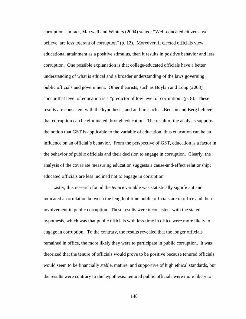
148

corruption. In fact, Maxwell and Winters (2004) stated: “Well-educated citizens, we

believe, are less tolerant of corruption” (p. 12). Moreover, if elected officials view

educational attainment as a positive stimulus, then it results in positive behavior and less

corruption. One possible explanation is that college-educated officials have a better

understanding of what is ethical and a broader understanding of the laws governing

public officials and government. Other theorists, such as Boylan and Long (2003),

concur that level of education is a “predictor of low level of corruption” (p. 8). These

results are consistent with the hypothesis, and authors such as Benson and Berg believe

that corruption can be eliminated through education. The result of the analysis supports

the notion that GST is applicable to the variable of education, thus education can be an

influence on an official’s behavior. From the perspective of GST, education is a factor in

the behavior of public officials and their decision to engage in corruption. Clearly, the

analysis of the covariate measuring education suggests a cause-and-effect relationship:

educated officials are less inclined not to engage in corruption.

Lastly, this research found the tenure variable was statistically significant and

indicated a correlation between the length of time public officials are in office and their

involvement in public corruption. These results were inconsistent with the stated

hypothesis, which was that public officials with less time in office were more likely to

engage in corruption. To the contrary, the results revealed that the longer officials

remained in office, the more likely they were to participate in public corruption. It was

theorized that the tenure of officials would prove to be positive because tenured officials

would seem to be financially stable, mature, and supportive of high ethical standards, but

the results were contrary to the hypothesis: tenured public officials were more likely to

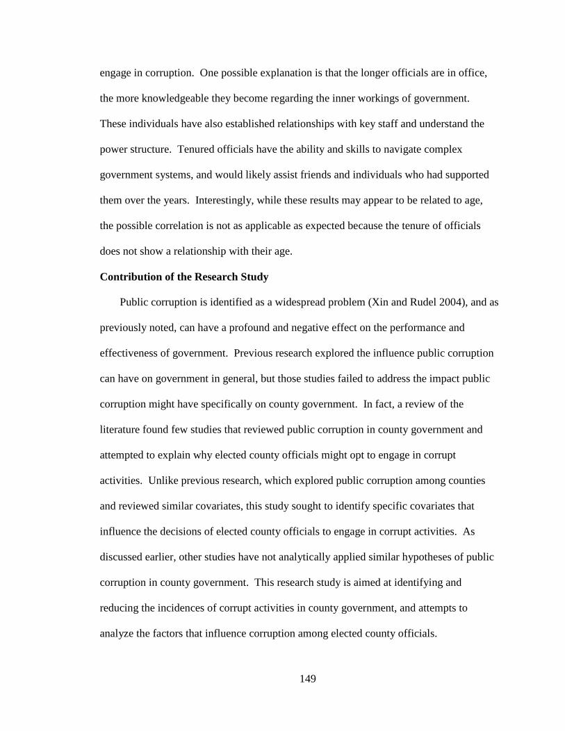
149

engage in corruption. One possible explanation is that the longer officials are in office,

the more knowledgeable they become regarding the inner workings of government.

These individuals have also established relationships with key staff and understand the

power structure. Tenured officials have the ability and skills to navigate complex

government systems, and would likely assist friends and individuals who had supported

them over the years. Interestingly, while these results may appear to be related to age,

the possible correlation is not as applicable as expected because the tenure of officials

does not show a relationship with their age.

Contribution of the Research Study

Public corruption is identified as a widespread problem (Xin and Rudel 2004), and as

previously noted, can have a profound and negative effect on the performance and

effectiveness of government. Previous research explored the influence public corruption

can have on government in general, but those studies failed to address the impact public

corruption might have specifically on county government. In fact, a review of the

literature found few studies that reviewed public corruption in county government and

attempted to explain why elected county officials might opt to engage in corrupt

activities. Unlike previous research, which explored public corruption among counties

and reviewed similar covariates, this study sought to identify specific covariates that

influence the decisions of elected county officials to engage in corrupt activities. As

discussed earlier, other studies have not analytically applied similar hypotheses of public

corruption in county government. This research study is aimed at identifying and

reducing the incidences of corrupt activities in county government, and attempts to

analyze the factors that influence corruption among elected county officials.

150

The contribution of this research study is significant because despite all previous

research conducted, public corruption remains a serious problem at all levels of

government. This research study not only contributes to the body of knowledge, it also

provides a good understanding of factors identified as contributors to corruption in

county government. It provides scholarly information for further studies and offers a

better understanding of why some elected officials opt to engage in acts of public

corruption and others do not.

Although this study compiled a great deal of information, all public officials cannot

be expected to fit the mold of all the characteristics identified here as factors in public

corruption. In fact, personal experience attests that some officials are inherently prone to

corrupt behavior. While the study produced good results and will add to the body of

knowledge on the subject, identifying those factors thought to contribute to public

corruption is not an exact science. However, the study does contribute to the scholarly

literature theorizing why public corruption exists in county government.

In addition, the significance of the variables identified in this study is worthy of

additional review and consideration; these variables, if implemented, could reduce the

influence of public corruption on county government and elected officials. The study

identified a number of factors, such as transparency, public participation, an educated

citizenry, media and public review, and effective disclosure laws and policies, that

influence the behavior and decisions of elected officials. Local governments that have

suffered cases of public corruption can provide excellent examples of the ways it

negatively influences service delivery, financial stability, public trust, and government

operations.

151

Conclusion

This research study found both governmental and individual profile characteristics

that predict public corruption in county government. Efforts have also been made to

ascertain the influence of GST on the corruption of county elected officials and county

government. This research study, along with GST, has provided a greater level of

understanding of the behavioral actions of elected public officials who choose to engage

in criminal activities, such as public corruption. As shown in this study, GST appears to

be a factor that induced elected officials to engage in public corruption, consistent with

the theoretical model. It is fair to conclude that the study found evidence that negative

strains exist and are an indicator of public corruption among elected officials.

Academic literature provided supporting explanations and justifications of how a

negative social environment, lack of educational attainment, and low financial

achievement are negative factors that influence the behavior and decisions of individuals.

The individuals in question here were elected county officials, who are no different from

any other citizens experiencing less-than-positive achievements; in these cases; however,

their behavior resulted in poor choices, such as engaging in corrupt behavior. The results

of the study suggest a positive correlation between public corruption and the environment

of public officials that, in many cases, can influence decisions and behavior. Not all the

covariates used in this study produced significant results, but the overall results produced

a substantial list of covariates that can be useful in predicting public corruption among

elected officials in large urban counties.

Although this research study is persuasive, additional research could improve the

overall model. The data used in this study could also be refined; conducting additional

152

research on state or city governments would provide supporting data and substantiate the

factors in this study identified as causes of public corruption. The data collected for this

study varied across states, but the results proved positive with a high rate of

predictability. Hence, the General Model for both county-level and individual-level

characteristics was successful in identifying factors that can be used to predict public

corruption.

If citizens demand an improved and honest government, reducing public corruption

becomes an important factor. The practical implication of this research study is primarily

the identification of factors that contribute to public corruption in county government and

among elected county officials in order to minimize corruption in county government.

This study identified nine factors that predicted public corruption, information that can be

used to deter corruption in county government. Improving the ability to predict

corruption can become a valuable tool in fighting it and restoring the public's trust in

government. The objective of this study was to identify possible factors that encourage

public corruption in county government, with the intention of creating a government

system that the public can trust and believe in. Rose-Ackerman (1999) believed that

“toleration of corruption in some areas of public life can facilitate a downward spiral in

which the malfeasance of some encourages more and more people to engage in

corruption over time” (p. 26).

Study Limitations

A few limitations were identified in this research study. First, the study did not

include individual data from county commissioners in counties with no cases of public

corruption. This lack of information limited the ability to analyze the effect personal

153

characteristics might have on the decisions of public officials to engage in corruption.

Including data from non-corrupt commissioners in non-corrupt counties could have been

useful when interpreting the results for the domain of individual predictors, and could

have provided a more diverse data set to understand the influence of individual predictors

when identifying factors that predict public corruption. The lack of this information also

influenced the requirement of generalizability. The General Model for individual-level

predictors is 76.1 percent, which is slightly weak compared to the results for county-level

data. The low results for individual-level prediction may be a result of the limited sample

size and the non-corruption limitation noted above. A larger number of corruption cases

could have greatly improved the overall model.

Second, several of the variables used in the study did not produce valid results for

determining corruption and, in the end, were not useful for analyzing the data. For

example, outside employment was not a valid indication of corruption; the data did not

produce meaningful results in which outside income could be used as a factor for

determining the likelihood of public corruption. Outside employment was originally

thought to be a covariate that would result in a positive outcome for public corruption,

but the data failed to produce the expected results. The overall wealth of commissioners

would have been more useful in determining public corruption. Open meeting laws were

another variable that did not pan out as a good indicator of public corruption. The laws

varied too widely among counties, making the information problematic to analyze.

Third, this study was limited to large urban counties with cases of public corruption,

which turned out to be 43 cases. A larger data set could have produced improved results,

even if the explanatory variables were not applicable to counties of less than 300,000. It

154

would be prudent to reevaluate some of the explanatory measurements to reflect

government size, as well as to provide additional opportunities to gather information

about the individual characteristics of elected officials in small counties.

Finally, much of the information about incarcerated elected officials was difficult to

obtain. The Justice Department’s process for obtaining information was not user-

friendly, which resulted in limited information even when public trials occurred.

Eventually all the information was obtained, but alternative data-gathering methods were

needed.

Further research in this area can address these shortcomings and develop a broad list

of explanatory measurements that could prove useful for later studies. While this study

provided good information and can serve as the first step for further studies, several new

predictive variables could help in identifying public corruption in county government.

This research study produced some good results in explaining some of the reasons elected

officials decided to engage in public corruption. If future researchers could establish a

relationship with the Justice Department or develop alternative methods for gathering

data about incarcerated officials, they might be able to collect more data on public

corruption in government.

Recommendations for Further Research

This research study successfully identified explanatory measurements of public

corruption, but there are opportunities for improvement that could benefit the field,

enhance further research, and reinforce and strengthen results. The findings described in

this study are useful in expanding scholarly knowledge and literature, although there are

155

limitations, as outlined above. However, changes to the study design might benefit

further research on the topic of public corruption.

First, undertaking a research study on public corruption was an enormous task.

Future research on the topic, with further identification of new explanatory measures,

might provide improved understanding and explanations of the influences of public

corruption on elected officials. For example, measures such as “family income” could

offer insight about the financial wealth of individuals and whether wealth is a valid

predictor for committing public corruption. A more in-depth analysis of anticorruption

policies should be included in future studies to determine the effectiveness of

enforcement policies and their impact on such components as conflict of interest policies,

gift-giving, and patronage. What impact could these policies have on curbing public

corruption in local government? The scope of review for this study on anticorruption

laws, such as ethics and open meeting laws, was limited to the strictness of the laws and

their influence on public corruption. Further studies on the effectiveness of these laws

and their role in curbing public corruption could be reviewed in future research. Political

campaign contributions and conflicts of interest are additional variables to include in

future studies; these added variables might explain the influence of campaigns and

political contributions on public corruption.

Second, a review of the findings suggests that adding domains to expand the scope of

the study or the areas of focus might improve the theoretical model and generate a better

understanding of public corruption. Additional domains might include a review of

private individuals involved in acts of public corruption, which could provide additional

insight into the potential for gain, as well as other motivations for acts of corruption.

156

What is the connection between private individuals and corruption among public

officials? What is the relationship between these two parties?

Third, further research on the media’s influence on public corruption could provide

useful information and aid in reducing corruption in government. Including the influence

of the media would provide an opportunity to assess opinions on what more could be

done from the media’s perspective when communicating to the public, reporting the

news, and providing information about the decisions and behavior of elected officials.

Expanding the study to include the domain of media would more accurately reflect its

impact and importance in identifying, deterring, and reporting corruption.

Fourth, further research should include assessing citizen opinions, possibly through

the use of a public opinion survey. Public opinion would provide an assessment of

government and its elected officials, along with critical information that could be useful

in developing recommendations for reducing corruption. Additionally, a public opinion

survey could gather information about the problems created by government corruption.

This information would be useful in gauging the objections and perceptions of the public

about how corruption influences the decisions of their elected officials.

Fifth, the use of this model is the initial process in determining if it was a reliable

tool in explaining public corruption. Further work is needed to establish the reliability of

the model—for instance, the study of public corruption in other government agencies.

An analysis of public corruption in city and state government, police departments, and

quasi-governmental agencies (e.g., water, sanitation, health, transportation) might be

beneficial.

157

Sixth, the research suggests that strain is perceived, but additional information would

have benefited the study. Personal interviews with elected officials would provide

greater insight to improve this aspect of the research study. Interviews would allow in-

depth questions to be asked of officials. This modification would improve the overall

study, since this change would allow the researcher to obtain specific information on

negative emotions, anger, negative behavior, social support structure, and financial

details.

Seventh, future research might further identify the influence term limits could have

on public corruption in county government. Recent voter-approved initiatives have

imposed limits on the length of time public officials can serve in elected positions. Some

of the arguments for enacting term limits are that they provide a check on concentration

of power, ensure long-term stability, and strengthen democracy. Research in this area

will broaden our knowledge and understanding of the influence term limits have on

increasing or decreasing public corruption in county government. It is recommended that

further research be undertaken to better understand their influence. Including this

variable would also allow a review of contract awards, campaign contributions, and

policy changes.

Finally, prior to any new research study, the General Models should be assessed and

refined to determine whether they accomplished the goals of predicting and explaining

public corruption. Further research in this area should include the removal or

modification of variables that did not produce valid results in order to improve the

study’s reliability in explaining public corruption within any government, regardless of

size or jurisdiction. Hence, it is suggested that future research studies on public

158

corruption include characteristics on private individuals, administrators, police officials,

city officials, state legislators, and federal officials. Expanding the research of public

corruption to include other elected officials will broaden our understanding of public

corruption, with the intent of developing and identifying profiles of characteristics that

can be used to identify individuals likely to engage in corrupt activities. Expanding the

research will provide opportunities to explore cause-and-effect relationships between

additional covariates and public corruption among a broader base of officials.

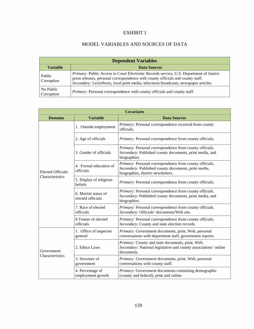
159

EXHIBIT I

MODEL VARIABLES AND SOURCES OF DATA

Dependent Variables Variable Data Sources

Public Corruption

Primary: Public Access to Court Electronic Records service, U.S. Department of Justice press releases, personal correspondence with county officials and county staff. Secondary: LexisNexis, local print media, television broadcasts, newspaper articles.

No Public Corruption Primary: Personal correspondence with county officials and county staff.

Covariates Domains Variable Data Sources

Elected Officials Characteristics

1. Outside employment Primary: Personal correspondence received from county officials.

2. Age of officials Primary: Personal correspondence from county officials.

3. Gender of officials Primary: Personal correspondence from county officials. Secondary: Published county documents, print media, and biographies.

4. Formal education of officials

Primary: Personal correspondence from county officials. Secondary: Published county documents, print media, biographies, district newsletters.

5. Display of religious beliefs Primary: Personal correspondence from county officials.

6. Marital status of elected officials

Primary: Personal correspondence from county officials. Secondary: Published county documents, print media, and biographies.

7. Race of elected officials

Primary: Personal correspondence from county officials. Secondary: Officials’ documents/Web site.

8.Tenure of elected officials

Primary: Personal correspondence from county officials. Secondary: County and state election records.


1. Office of inspector general

Primary: Government documents, print, Web, personal conversations with department staff, government reports.

2. Ethics Laws Primary: County and state documents, print, Web. Secondary: National legislative and county associations’ online documents.

3. Structure of government

Primary: Government documents, print, Web, personal conversations with county staff.

4. Percentage of employment growth

Primary: Government documents containing demographic (county and federal), print and online.

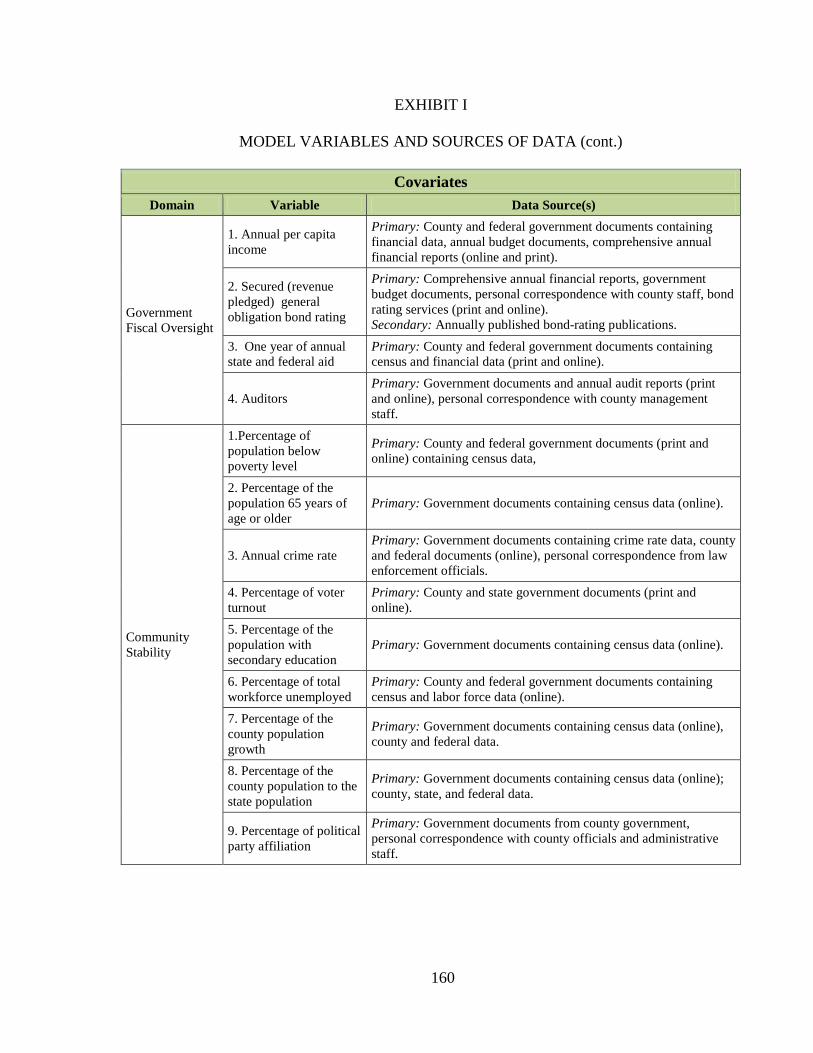
160

EXHIBIT I

MODEL VARIABLES AND SOURCES OF DATA (cont.)

Covariates Domain Variable Data Source(s)

Government Fiscal Oversight

1. Annual per capita income

Primary: County and federal government documents containing financial data, annual budget documents, comprehensive annual financial reports (online and print).

2. Secured (revenue pledged) general obligation bond rating

Primary: Comprehensive annual financial reports, government budget documents, personal correspondence with county staff, bond rating services (print and online). Secondary: Annually published bond-rating publications.

3. One year of annual state and federal aid

Primary: County and federal government documents containing census and financial data (print and online).

4. Auditors Primary: Government documents and annual audit reports (print and online), personal correspondence with county management staff.

Community Stability

1.Percentage of population below poverty level

Primary: County and federal government documents (print and online) containing census data,

2. Percentage of the population 65 years of age or older

Primary: Government documents containing census data (online).

3. Annual crime rate Primary: Government documents containing crime rate data, county and federal documents (online), personal correspondence from law enforcement officials.

4. Percentage of voter turnout

Primary: County and state government documents (print and online).

5. Percentage of the population with secondary education

Primary: Government documents containing census data (online).

6. Percentage of total workforce unemployed

Primary: County and federal government documents containing census and labor force data (online).

7. Percentage of the county population growth

Primary: Government documents containing census data (online), county and federal data.

8. Percentage of the county population to the state population

Primary: Government documents containing census data (online); county, state, and federal data.

9. Percentage of political party affiliation

Primary: Government documents from county government, personal correspondence with county officials and administrative staff.

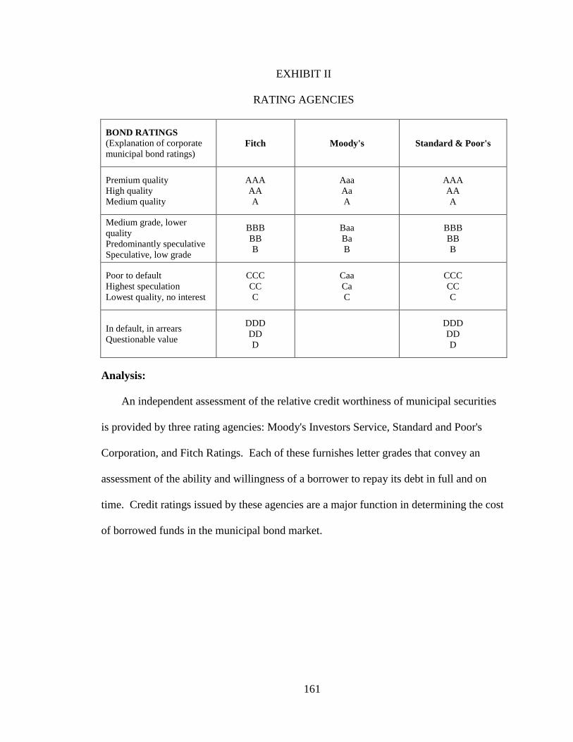
161

EXHIBIT II

RATING AGENCIES

BOND RATINGS (Explanation of corporate municipal bond ratings)

Fitch Moody's Standard & Poor's

Premium quality High quality Medium quality

AAA AA A

Aaa Aa A

AAA AA A

Medium grade, lower quality Predominantly speculative Speculative, low grade

BBB BB B

Baa Ba B

BBB BB B

Poor to default Highest speculation Lowest quality, no interest

CCC CC C

Caa Ca C

CCC CC C

In default, in arrears Questionable value

DDD DD D

DDD DD D

Analysis:

An independent assessment of the relative credit worthiness of municipal securities

is provided by three rating agencies: Moody's Investors Service, Standard and Poor's

Corporation, and Fitch Ratings. Each of these furnishes letter grades that convey an

assessment of the ability and willingness of a borrower to repay its debt in full and on

time. Credit ratings issued by these agencies are a major function in determining the cost

of borrowed funds in the municipal bond market.

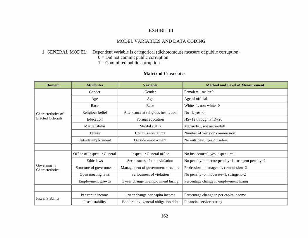
162

EXHIBIT III

MODEL VARIABLES AND DATA CODING

1. GENERAL MODEL: Dependent variable is categorical (dichotomous) measure of public corruption. 0 = Did not commit public corruption 1 = Committed public corruption

Matrix of Covariates

Domain Attributes Variable Method and Level of Measurement

Characteristics of Elected Officials

Gender Gender Female=1, male=0

Age Age Age of official

Race Race White=1, non-white=0

Religious belief Attendance at religious institution No=1, yes=0

Education Formal education HS=12 through PhD=20

Marital status Marital status Married=1, not married=0

Tenure Commission tenure Number of years on commission

Outside employment Outside employment No outside=0, yes outside=1


Office of Inspector General Inspector General office No inspector=0, yes inspector=1

Ethic laws Seriousness of ethic violation No penalty/moderate penalty=1, stringent penalty=2

Structure of government Management of government structure Professional manager=1, commission=2

Open meeting laws Seriousness of violation No penalty=0, moderate=1, stringent=2

Employment growth 1 year change in employment hiring Percentage change in employment hiring

Fiscal Stability Per capita income 1 year change per capita income Percentage change in per capita income

Fiscal stability Bond rating; general obligation debt Financial services rating

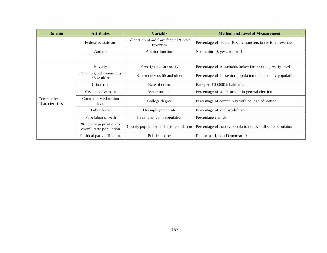
163

Domain Attributes Variable Method and Level of Measurement

Federal & state aid Allocation of aid from federal & state revenues Percentage of federal & state transfers to the total revenue

Auditor Auditor function No auditor=0, yes auditor=1


Poverty Poverty rate for county Percentage of households below the federal poverty level Percentage of community

65 & older Senior citizens 65 and older Percentage of the senior population to the county population

Crime rate Rate of crime Rate per 100,000 inhabitants

Civic involvement Voter turnout Percentage of voter turnout in general election Community education

level College degree Percentage of community with college education

Labor force Unemployment rate Percentage of total workforce

Population growth 1 year change in population Percentage change % county population to overall state population County population and state population Percentage of county population to overall state population

Political party affiliation Political party Democrat=1, non-Democrat=0

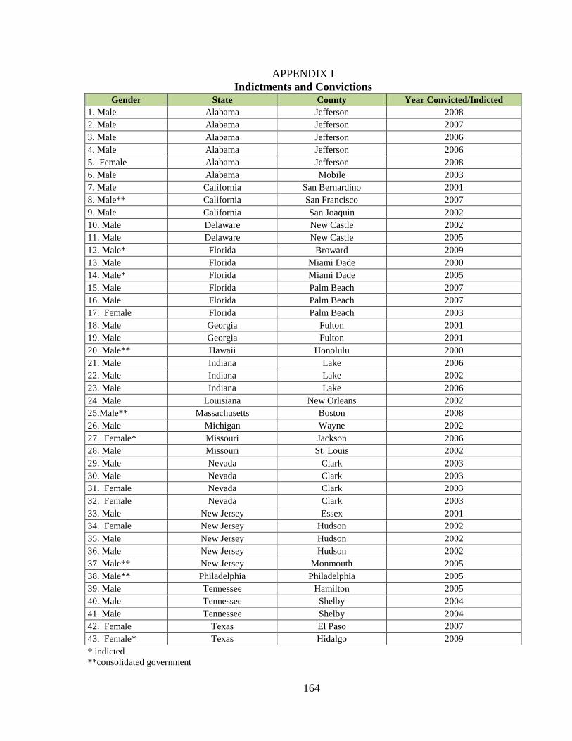
164

APPENDIX I Indictments and Convictions

Gender State County Year Convicted/Indicted 1. Male Alabama Jefferson 2008 2. Male Alabama Jefferson 2007 3. Male Alabama Jefferson 2006 4. Male Alabama Jefferson 2006 5. Female Alabama Jefferson 2008 6. Male Alabama Mobile 2003 7. Male California San Bernardino 2001 8. Male** California San Francisco 2007 9. Male California San Joaquin 2002 10. Male Delaware New Castle 2002 11. Male Delaware New Castle 2005 12. Male* Florida Broward 2009 13. Male Florida Miami Dade 2000 14. Male* Florida Miami Dade 2005 15. Male Florida Palm Beach 2007 16. Male Florida Palm Beach 2007 17. Female Florida Palm Beach 2003 18. Male Georgia Fulton 2001 19. Male Georgia Fulton 2001 20. Male** Hawaii Honolulu 2000 21. Male Indiana Lake 2006 22. Male Indiana Lake 2002 23. Male Indiana Lake 2006 24. Male Louisiana New Orleans 2002 25.Male** Massachusetts Boston 2008 26. Male Michigan Wayne 2002 27. Female* Missouri Jackson 2006 28. Male Missouri St. Louis 2002 29. Male Nevada Clark 2003 30. Male Nevada Clark 2003 31. Female Nevada Clark 2003 32. Female Nevada Clark 2003 33. Male New Jersey Essex 2001 34. Female New Jersey Hudson 2002 35. Male New Jersey Hudson 2002 36. Male New Jersey Hudson 2002 37. Male** New Jersey Monmouth 2005 38. Male** Philadelphia Philadelphia 2005 39. Male Tennessee Hamilton 2005 40. Male Tennessee Shelby 2004 41. Male Tennessee Shelby 2004 42. Female Texas El Paso 2007 43. Female* Texas Hidalgo 2009 * indicted **consolidated government

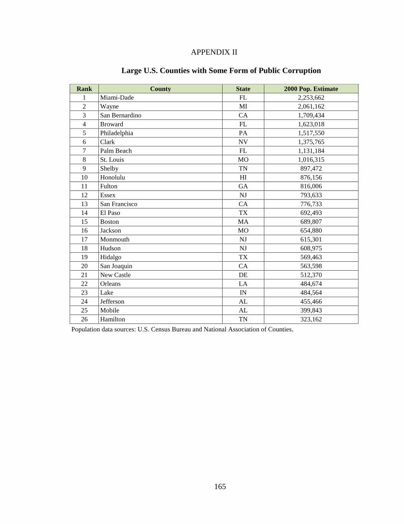
165

APPENDIX II

Large U.S. Counties with Some Form of Public Corruption

Rank County State 2000 Pop. Estimate 1 Miami-Dade FL 2,253,662 2 Wayne MI 2,061,162 3 San Bernardino CA 1,709,434 4 Broward FL 1,623,018 5 Philadelphia PA 1,517,550 6 Clark NV 1,375,765 7 Palm Beach FL 1,131,184 8 St. Louis MO 1,016,315 9 Shelby TN 897,472 10 Honolulu HI 876,156 11 Fulton GA 816,006 12 Essex NJ 793,633 13 San Francisco CA 776,733 14 El Paso TX 692,493 15 Boston MA 689,807 16 Jackson MO 654,880 17 Monmouth NJ 615,301 18 Hudson NJ 608,975 19 Hidalgo TX 569,463 20 San Joaquin CA 563,598 21 New Castle DE 512,370 22 Orleans LA 484,674 23 Lake IN 484,564 24 Jefferson AL 455,466 25 Mobile AL 399,843 26 Hamilton TN 323,162

Population data sources: U.S. Census Bureau and National Association of Counties.

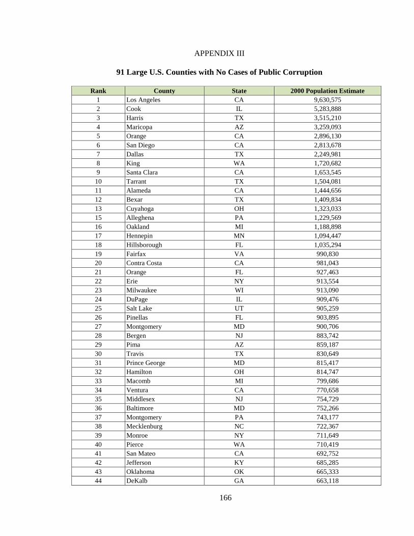
166

APPENDIX III

91 Large U.S. Counties with No Cases of Public Corruption

Rank County State 2000 Population Estimate 1 Los Angeles CA 9,630,575 2 Cook IL 5,283,888 3 Harris TX 3,515,210 4 Maricopa AZ 3,259,093 5 Orange CA 2,896,130 6 San Diego CA 2,813,678 7 Dallas TX 2,249,981 8 King WA 1,720,682 9 Santa Clara CA 1,653,545

10 Tarrant TX 1,504,081 11 Alameda CA 1,444,656 12 Bexar TX 1,409,834 13 Cuyahoga OH 1,323,033 15 Alleghena PA 1,229,569 16 Oakland MI 1,188,898 17 Hennepin MN 1,094,447 18 Hillsborough FL 1,035,294 19 Fairfax VA 990,830 20 Contra Costa CA 981,043 21 Orange FL 927,463 22 Erie NY 913,554 23 Milwaukee WI 913,090 24 DuPage IL 909,476 25 Salt Lake UT 905,259 26 Pinellas FL 903,895 27 Montgomery MD 900,706 28 Bergen NJ 883,742 29 Pima AZ 859,187 30 Travis TX 830,649 31 Prince George MD 815,417 32 Hamilton OH 814,747 33 Macomb MI 799,686 34 Ventura CA 770,658 35 Middlesex NJ 754,729 36 Baltimore MD 752,266 37 Montgomery PA 743,177 38 Mecklenburg NC 722,367 39 Monroe NY 711,649 40 Pierce WA 710,419 41 San Mateo CA 692,752 42 Jefferson KY 685,285 43 Oklahoma OK 665,333 44 DeKalb GA 663,118

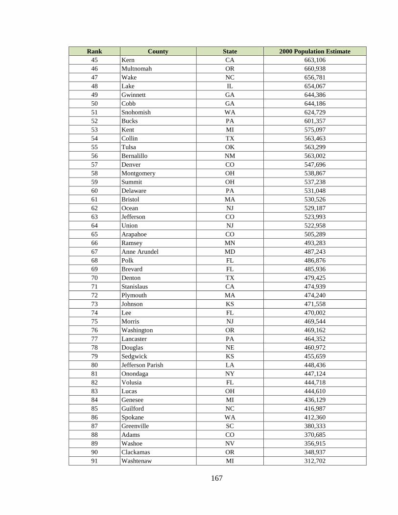
167

Rank County State 2000 Population Estimate 45 Kern CA 663,106 46 Multnomah OR 660,938 47 Wake NC 656,781 48 Lake IL 654,067 49 Gwinnett GA 644,386 50 Cobb GA 644,186 51 Snohomish WA 624,729 52 Bucks PA 601,357 53 Kent MI 575,097 54 Collin TX 563,463 55 Tulsa OK 563,299 56 Bernalillo NM 563,002 57 Denver CO 547,696 58 Montgomery OH 538,867 59 Summit OH 537,238 60 Delaware PA 531,048 61 Bristol MA 530,526 62 Ocean NJ 529,187 63 Jefferson CO 523,993 64 Union NJ 522,958 65 Arapahoe CO 505,289 66 Ramsey MN 493,283 67 Anne Arundel MD 487,243 68 Polk FL 486,876 69 Brevard FL 485,936 70 Denton TX 479,425 71 Stanislaus CA 474,939 72 Plymouth MA 474,240 73 Johnson KS 471,558 74 Lee FL 470,002 75 Morris NJ 469,544 76 Washington OR 469,162 77 Lancaster PA 464,352 78 Douglas NE 460,972 79 Sedgwick KS 455,659 80 Jefferson Parish LA 448,436 81 Onondaga NY 447,124 82 Volusia FL 444,718 83 Lucas OH 444,610 84 Genesee MI 436,129 85 Guilford NC 416,987 86 Spokane WA 412,360 87 Greenville SC 380,333 88 Adams CO 370,685 89 Washoe NV 356,915 90 Clackamas OR 348,937 91 Washtenaw MI 312,702

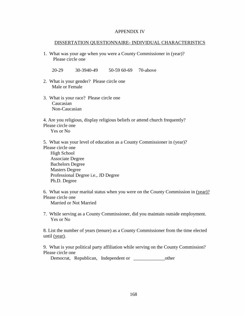
168

APPENDIX IV

DISSERTATION QUESTIONNAIRE- INDIVIDUAL CHARACTERISTICS

1. What was your age when you were a County Commissioner in (year)? Please circle one

20-29 30-39 40-49 50-59 60-69 70-above

2. What is your gender? Please circle one Male or Female

3. What is your race? Please circle one Caucasian Non-Caucasian

4. Are you religious, display religious beliefs or attend church frequently? Please circle one

Yes or No

5. What was your level of education as a County Commissioner in (year)? Please circle one

High School Associate Degree Bachelors Degree Masters Degree Professional Degree i.e., JD Degree Ph.D. Degree

6. What was your marital status when you were on the County Commission in (year)? Please circle one

Married or Not Married

7. While serving as a County Commissioner, did you maintain outside employment. Yes or No

8. List the number of years (tenure) as a County Commissioner from the time elected until (year).

9. What is your political party affiliation while serving on the County Commission? Please circle one

Democrat, Republican, Independent or _____________other

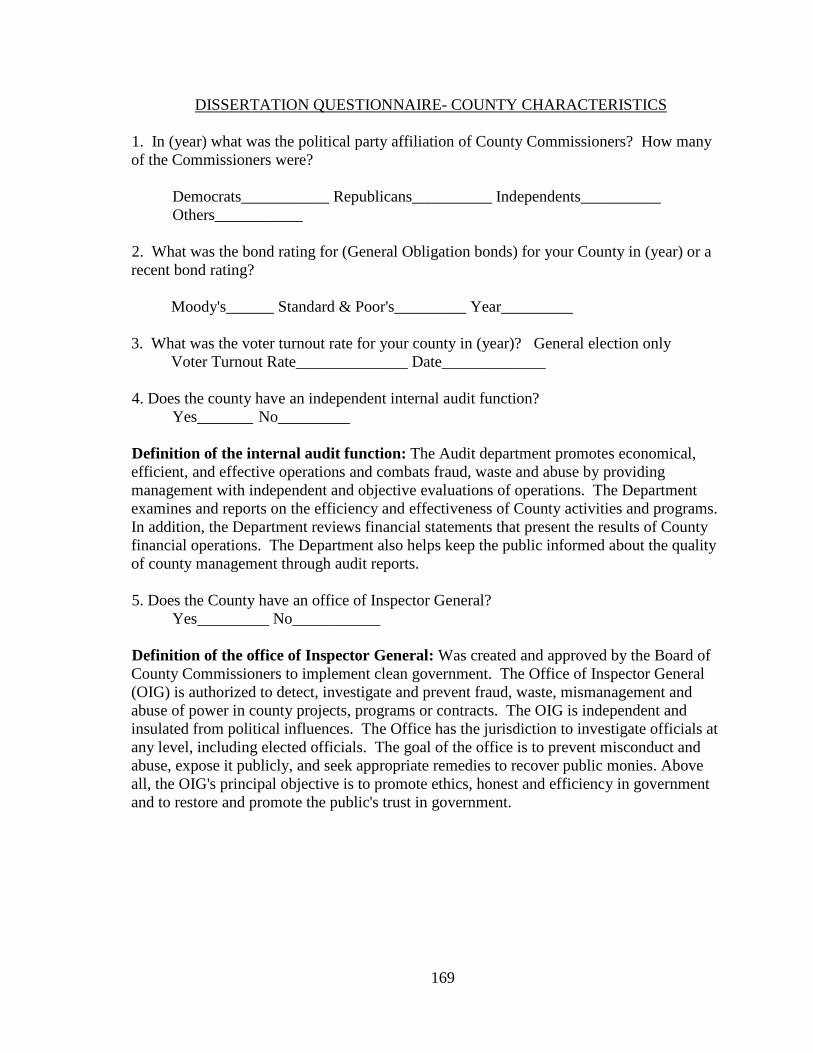
169

DISSERTATION QUESTIONNAIRE- COUNTY CHARACTERISTICS

1. In (year) what was the political party affiliation of County Commissioners? How many of the Commissioners were?

Democrats___________ Republicans__________ Independents__________ Others___________

2. What was the bond rating for (General Obligation bonds) for your County in (year) or a recent bond rating?

Moody's______ Standard & Poor's_________ Year_________

3. What was the voter turnout rate for your county in (year)? General election only Voter Turnout Rate______________ Date_____________

4. Does the county have an independent internal audit function? Yes_______ No_________

Definition of the internal audit function: The Audit department promotes economical, efficient, and effective operations and combats fraud, waste and abuse by providing management with independent and objective evaluations of operations. The Department examines and reports on the efficiency and effectiveness of County activities and programs. In addition, the Department reviews financial statements that present the results of County financial operations. The Department also helps keep the public informed about the quality of county management through audit reports.

5. Does the County have an office of Inspector General? Yes_________ No___________

Definition of the office of Inspector General: Was created and approved by the Board of County Commissioners to implement clean government. The Office of Inspector General (OIG) is authorized to detect, investigate and prevent fraud, waste, mismanagement and abuse of power in county projects, programs or contracts. The OIG is independent and insulated from political influences. The Office has the jurisdiction to investigate officials at any level, including elected officials. The goal of the office is to prevent misconduct and abuse, expose it publicly, and seek appropriate remedies to recover public monies. Above all, the OIG's principal objective is to promote ethics, honest and efficiency in government and to restore and promote the public's trust in government.

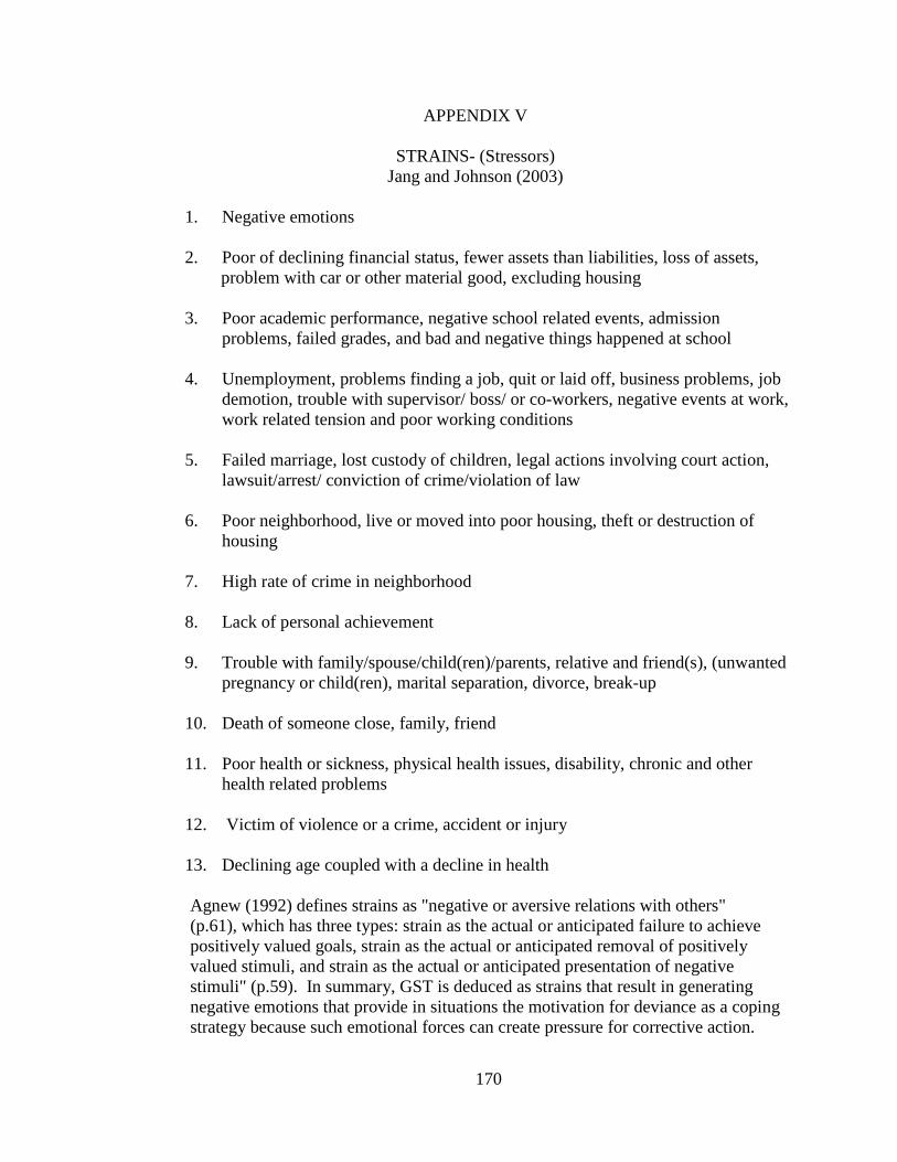
170

APPENDIX V

STRAINS- (Stressors) Jang and Johnson (2003)

1. Negative emotions

2. Poor of declining financial status, fewer assets than liabilities, loss of assets, problem with car or other material good, excluding housing

3. Poor academic performance, negative school related events, admission

problems, failed grades, and bad and negative things happened at school 4. Unemployment, problems finding a job, quit or laid off, business problems, job

demotion, trouble with supervisor/ boss/ or co-workers, negative events at work, work related tension and poor working conditions

5. Failed marriage, lost custody of children, legal actions involving court action,

lawsuit/arrest/ conviction of crime/violation of law 6. Poor neighborhood, live or moved into poor housing, theft or destruction of housing 7. High rate of crime in neighborhood

8. Lack of personal achievement

9. Trouble with family/spouse/child(ren)/parents, relative and friend(s), (unwanted pregnancy or child(ren), marital separation, divorce, break-up

10. Death of someone close, family, friend

11. Poor health or sickness, physical health issues, disability, chronic and other health related problems

12. Victim of violence or a crime, accident or injury 13. Declining age coupled with a decline in health

Agnew (1992) defines strains as "negative or aversive relations with others" (p.61), which has three types: strain as the actual or anticipated failure to achieve positively valued goals, strain as the actual or anticipated removal of positively valued stimuli, and strain as the actual or anticipated presentation of negative stimuli" (p.59). In summary, GST is deduced as strains that result in generating negative emotions that provide in situations the motivation for deviance as a coping strategy because such emotional forces can create pressure for corrective action.

171

REFERENCES

Allen, D. W. 2002. Corruption, scandal, and political economy of adopting lobbying policies: An exploratory assessment. Public Integrity, IV(I), 13-41.

Amundsen, I. 1999. Political corruption: An introduction to the issues. Chq. Mighelsen Institute Development Studies and Human Rights,

Agnew, R. 1985. A revised strain theory of delinquency. Social Forces, 64(1), 151-167.

———. 1992. Foundation for a general strain theory of crime and delinquency. Criminology, 30(1), 24-87.

———. 1999. A General Strain Theory of community differences in crime rates. Journal of Research in Crime and Delinquency, 36, 123-155.

———. 2001. Building on the foundation of General Strain Theory: Specifying the types of strain most likely to lead to crime and delinquency. Journal of Research in Crime and Delinquency, 38, 319-361.

Agnew, R., T. Brezina, F. T. Cullen, and J. P. Wright. 2002. Strain, personality traits, and delinquency: Extending General Strain Theory. Criminology, 40(1), 43-71.

Agnew, R., and H.R. White. 1992. An empirical test of general strain theory. Criminology, 30, 475-499.

Alam, M. S. 1995. A theory of limits on corruption and same applications. Kyklos, 48, 419-435.

Alesina, A., R. Baqir, and E. William. 2002. Redistribution Public Employment, Journal of Urban Economics, 48, 219-241.

Anechiarico, F., and J. B. Jacobs. 1996. The Pursuit of Absolute Integrity: How Corruption Control Makes Government Ineffective. Chicago: University of Chicago Press.

Arrow, K. 1971. Essays in the Theory of Risk Bearing. Chicago: Markham.

Aseltine, R. H., S. Gore. and J. Gordon. 2000. Life stress, anger and anxiety, and delinquency: An empirical test of General Strain Theory. Journal of Health and Social Behavior, 41, 256-275.

Averill, J. R. 1982. Anger and Aggression. New York: Springer-Verlag.

Azfar O., Y. Lee, and A. Swamy. 2001. The causes and consequences of corruption. American Academy of Political and Social Science, 573, Culture and Development: International Perspective, 42-56.

172

Banerjee, A. 1997. A theory of misgovernance. The Quarterly Journal of Economics, 112(4), 1289-1332.

Bandfield, E. C. 1958. The Moral Basis of a Backward Society. New York, NY: Free Press.

Bardhan, P. 1997. Corruption and development: A review of issues. Journal of Economic Literature, 35(3), 1320-1346.

Baron, S. W. 2003. Self-control, social consequences, and criminal behavior: Street youth and the General Theory of Crime. Journal of Research in Crime and Delinquency, 40, 403-425.

Benson, G. C.S. 1978. Political Corruption in America. Lexington Books D.C.: Heath and Company Lexington, Massachusetts; Toronto.

Berg, L. L., H. Hahn, and J. R. Schmidhauser. 1976. Corruption in the American Political System. Morristown. N.J.: General Learning Press.

Berkowitz, L. 1982. Aversive conditions as stimuli to aggression. In Advances in Experimental Social Psychology, ed. Leonard Berkowitz, 15. New York: Academic Press.

Georges Bernanos. (n.d.). BrainyQuote.com. Retrieved December 12, 2009, from BrainyQuote.com Web site: http://www.brainyquote.com/quotes/quotes/g/georgesber149409.html

Bernard, T. J. 1987. Testing structural strain theory. Journal of Research in Crime and Delinquency, 24, 262-280.

Besley, T., and J. McLaren. 1993. Taxes and bribery: The role of wage incentives. The Economic Journal, 103(416), 119-141.

Boniolo, P., and R. Elbert. 2005. A working class theory of corruption: Thematic analysis of workers’ ideas about corruption and its consequences, Urbana- Champaign,

Boylan, R. T., and C. X. Long. 2003. Measuring public corruption in the american states: A survey of statehouse reporters. State Politics and Policy Quarterly, 3(4), 420-438.

Broidy, L. 2001. A test of General Strain Theory. Criminology, 39, 9-34.

Brooks, R. C. 1909. The nature of political corruption. Political Science Quarterly, 24(1), 1-22.

Cabelkova, I., and J. Hanousek. 2004. The power of negative thinking: Corruption, perception and willingness to bribe in Ukraine. Applied Economics, 36(4), 383-397.

173

Cadot, O. 1987. Corruption as a gamble. Journal of Public Economics, 33(2), 223-244.

Caiden, G. E. (1988). Toward a general theory of official corruption. Asian Journal of Public Administration, 10(1), 1-24.

Cohen, A. K. 1995. Delinquent Boys: The Culture of the Gang Glencoe. New York: Free Press.

———. 1965. The sociology of the deviant act: Anomie theory and beyond. American Sociological Review, 30, 5-14.

Cohen, A. K., and J. Short. 1958. Research in delinquent subcultures. Journal of Social Issues, 20-37.

Coleman, J. 1995. Motivation and opportunity: Understanding the causes of white-collar crime. In White Collar Crime, 3rd edition. Ed. G. Geis, R. Meier, and L. Salinger. 360-381. New York: Free Press.

Collier, M. W. 1999. Explaining political corruption: An institutional-choice approach. Florida International University, http://www.ciaonet.org/isa/com01/ (accessed 10/12/09).

Cloward, R., and L. Ohlin. 1960. Delinquency and Opportunity: A Theory of Delinquent Gangs. New York: Free Press.

Croall, H. 2001. Understanding White Collar Crime. Buckingham, UK: Open University Press.

De Leon, P. 1993. Thinking about Political Corruption. Armonk: M. E. Sharpe.

della Porta, D. 1996. Actors in Corruption: Business Politicians in Italy. ISSJ 149/1996. Cambridge, MA: Blackwell Publishers.

della Porta, D., and A. Vannucci. 1999. Corruption Exchange: Actors, Resources, and Mechanisms of Political Corruption. New York: Walter de Gruyter.

della Porta, D., A. Pizzorno, and J. Donaldson. 1996. The business politicians: Reflections from a study of political corruption. Politics of Corruption, pp. 73-94.

Dexter, L.A. 1993. Complexities of corruption. Society, 30(4), 63-64.

Dollar, D., R. Fisman, and R. Gatti. 1999. Are women really the ‘fairer’ sex? Corruption and women in government. Policy Research Report on Gender and Development Working Paper Series, No. 4. Washington, D.C.: World Bank.

Dresang, D. L. 2003. Mr. Clean gets dirty: The demise of public ethics in Wisconsin. Public Integrity, 5(4), 319-353.

174

Dreyer, W. J. 2007. Defending a public official against charges of public corruption in the United States and the model case of United States of America V. McDonough. American Bar Association. http://apps.americanbar.org/rol/publications/asia_raca_mr_dreyer_ defending_official.pdf. Accessed 10/12/09.

Eisenhardt, K. M. 1989. Agency Theory: An assessment and review. The Academy of Management Review, 14(1), 57-74.

Elliott, D., S. Ageton, and R. Canter. 1979. An integrated theoretical perspective on delinquent behavior. Journal of Research in Crime and Delinquency, 16, 3-27.

Elliott, D., and H. Voss. 1974. Delinquency and Dropout. Lexington, MA: Lexington Books.

Elliott, D., D. Huizinga, and S. Ageton. 1985. Explaining Delinquency and Drug Use. Beverly Hills, California: Sage.

Empey, L. 1982. American Delinquency: Its Meaning and Construction. Homewood, IL: Dorsey.

Evans, D. T., F. T. Cullen, V. S. Burton, G. Dunaway, and M. L. Benson. 1997. The social consequences of self-control: Testing the general theory of crime. Criminology 35, 475-501.

Fischer, C. 1995. The subcultural theory of urbanism: A twentieth year assessment. American Journal of Sociology, 101(3), 543-577.

Ford, R. C., and D. R. Woodrow. 1994. Ethical decision-making: A review of the empirical literature. Journal of Business Ethics, 13, 205-221.

Friedrich, C. J. 1966. Political pathology. The Political Quarterly, 37, 70-85.

———. 1989. Corruption concepts in historical perspectives. In Political Corruption: A Handbook, ed. A. J. Heidenheimer, M. Johnson, and V. T. LeVine, 15-24. New Brunswick, NJ: Transaction Books.

Fuchs, H. W. 1986. Auditing as a political instrument. In Fraud, Waste and Abuse in Government, ed. Jerome B. McKinney and Michael Johnson. Philadelphia: ISHI Publications.

Gallup International Millennium Survey. 1998. http://www. gallup-international.com/ survey5.htm. Accessed 10/07/09.

Gardiner, J. A., and T. R. Lyman. 1990. The logic of corruption control. In Political Corruption: A Handbook, ed. A. J. Heidenheimer, M. Johnson, and V. T. LeVine, 827-840. New Brunswick, NJ: Transaction Books.

175

Glaeser, E. L., and R. Saks. 2004. Corruption in America. Harvard Institute of Economic Research, 2043, 1-23.

Glaeser, E.L., D. I. Laibson, J.A. Scheinkman, and C. L. Soutter. 2000. Measuring trust. The Quarterly Journal of Economics, 115(3), 811-846.

Glor, E. D., and I. Greene. 2002. The government of Canada’s approach to ethics: The evolution of ethical government. Public Integrity, 5(1), 40-65.

Glover, S. H., M.A. Bumpus, J.E. Logan, and J. R. Ciesla. 1997. Reexaming the influence of individual values on ethical decision-making. Journal of Business Ethnics, 16, 1316-1329.

Goel, R. K., and M. A. Nelson. 1998. Corruption and government size: A disaggregated analysis. Public Choice, XCVII, 107-120.

Gottfredson, M. and T. Hirchi. 1990. A General Theory of Crime. Stanford: Stanford University Press.

Gould, D., and J. Amaro-Reyes.1983. The Effects of Corruption on Administrative Performance: Illustrations from Developing Countries. Staff Working Paper 580. Washington, D.C.: World Bank.

Graaf, G., and L. W. J. C. Huberts. 2008. Portraying the nature of corruption using an explorative case study design. Public Administration Review, 640-653.

Grasmick, H. G., C. R. Tittle, R. J. Bursik Jr., and B. J. Arneklev. 1993. Testing the care: Empirical implication of Gottfredson and Hirschi’s General Theory of Crime. Journal Resources Crime Delinquency, 30, 5-29.

Greenberg, D. F. 1977. Delinquency and the age structure of society. Contemporary Crises, 1, 189-223.

Greenstein, F. I. 1964. The changing pattern of urban party politics. Annals of the American Academy of Political & Social Science, 353, 1-13.

Hagan, J., and R. D. Peterson. 1995. Criminal inequality in America: Patterns and consequences. In Crime and Inequality, ed. J. Hogan and R. D. Peterson, 14-36. Stanford: Stanford University Press.

Haines, D. W. 2003. Fatal choices: The routinization of deceit, incompetence, and corruption. Public Integrity, 6(1), 5-38.

Heidenheimer, A. J. 1989a. Perspectives on the perception of corruption. In Political Corruption: A Handbook, ed. A. J. Heidenheimer, M. Johnson, and V. T. LeVine, 149-163. New Brunswick, NJ: Transaction Books.

176

Heywood, P. 1997. Political corruption: Problems and perspectives. Political Studies, XLV, 417-435.

Hill, K. Q. 2003. Democratization and corruption: Systematic evidence from the American states. American Politics Research, 31, 613-631.

Hopkins, W. G. 2000. Quantitative Research Design. http://www.sportsci.org/jour/0001/ wghdesign.html. Accessed 10/05/09.

Huffington, A. 2003. Pigs at the Trough: How Corporate Greed and Political Corruption Are Undermining America. New York: Crown Publishers.

Hunt, J. 2004. Trust and bribery: The role of the quid pro quo and the like with crime. National Bureau of Economic Research, Discussion Paper 10510.

———. 2005. Why are some public officials more corrupt than others? National Bureau of Economic Research, Discussion Paper 11595.

———. 2006. How corruption hits people when they are down. National Bureau of Economic Research, Discussion Paper 12490.

Huntington, S. 1968. Political Order in Changing Societies. New Haven: Yale University Press.

Husted, B. W. 1999. Wealth, culture, and corruption. Journal of International Business Studies, 30(2), 339-359.

Jacquemet, N. 2006. “Corruption as Betrayal: Experimental Evidence.” Working paper 0506. Groupe d'Analyse et de Théorie Economique, Centre national de la recherche scientifique, Université Lyon 2, Ecole Normale Supérieure.

Jang, S. J. and B. R. Johnson. 2003. Strain, negative emotions, and deviant coping among African-Americans: A test of General Strain Theory. Journal of Quantitative Criminology, 19(1), 79-105.

Jain, A. K. 2001. Corruption: A review. Journal of Economic Surveys, 15(1), 71-121.

Jensen, M. C. 1994. Self-Interest, altruism, incentives and Agency Theory. Journal of Applied Corporate Finance, VII (2), 1-16.

Joaquin, E. T. 2004. Decentralization and corruption: The bumpy road to public sector integrity in developing countries. A Journal of the American Society for Public Administration, 6(3), 207-219.

Johnson, M. 1982. Political Corruption and Public Policy in America. Monterey, CA: Brooks/Cole Publishing Company.

177

Johnson, M. 1983. Corruption and political culture: An empirical perspective. Publius, 13, 1 (Winter): 19-39.

Johnson, M. 1996. The search for definitions: The vitality of politics and the issue of corruption. International Social Science Journal, 48(3), 321-335.

Jones, S., and N. Quisenberry. 2004. The General Theory of crime: how general is it? Deviant Behavior, 25, 401-426.

Kaufmann, D. 1997. Corruption: The facts. Foreign Policy, Summer: 114-131.

Kemper, T. D. 1978. A Social Interactional Theory of Emotion. New York: John Wiley and Sons.

Ketti, D. F. 2006. Shedding light on corruption. http://www.america.gov/st/demoracy- english/2008/may/20080601225050SrenoD9.353274e-02.html. Accessed 09/17/09.

Key, V.O. Jr. 1936. Techniques of political graft in the United States. In Political Corruption: A Handbook, ed. A. J. Heidenheimer, M. Johnson, and V. T. LeVine, 39-49. New Brunswick, NJ: Transaction Books.

King, G., R. O. Keohane, and V. Sidney. 1994. Designing Social Inquiry. Princeton: University Press.

Kingston, C. 2003. Social structure, collective action, and corruption: Theory, and evidence from India. http://ipl.econ.duke.edu/bread/papers/041604_Conference/kingston.pdf. Accessed 09/11/09.

———. 2005. Social capital and corruption: Theory, and evidence from India. http://www3.amherst.edu/~cgkingston/India.pdf. Accessed 09/11/09.

Klitgarrd, R. 1988. Controlling Corruption. Berkeley: University of California Press.

Kluegel, R. L., and D. Heise. 1986. Beliefs about Inequality. New York: Aldine De Gryter.

Kobrin, J. A. 2006. Betraying honest services: Theories of trust and betrayal applied to the mail fraud statues and § 1346. In NYU Annual Survey of American Law, ed. J. A. Korbin, 779-795. http://www.law.nyu.edu/ecm_dlv1/groups/public/@nyu_law_website__journals__ annual_survey_of_american_law/documents/documents/ecm_pro_064637.pdf. Accessed 09/12/09.

178

Kohlberg, L. 1973. Continuities in childhood and adult development revisited. In Kohlberg: Collected Papers on Moral Development and Moral Education. Cambridge, MA: Center for Moral Development, Harvard University.

La Palombara, J. 1994. Structural and institutional aspects of corruption. Social Research, LXI, 325-350.

La Porta, R., F. Lopez de-Silanes, A. Shleifer, and R. W. Vishny. 1999. The quality of government. Journal of Law, Economics and Organization 15(1), 222-279.

———. 1997. Truth in large organizations. American Economic Review, paper and proceedings, CXXXVII (2), 333-338.

LaGrange, T.C., and R. A. Silverman. 1999. Low self-control and opportunity: Testing the General Theory of Crime as an explanation for gender differences in delinquency. Criminology, 37(1), 41-72.

Lambsdorff, J.G. 1999. Corruption in empirical research: A review. Working paper. http://gwdu05.gwdg.de/~uwvw/downloads/contribution05_lambsdorff.pdf. Accessed 09/12/09.

——— 2000. Corruption Perception Index. Working paper. Berlin: Transparency International.

——— 2001. How corruption in government affects public welfare: A review of theories. Center for Globalization and Europeanization of the Economy, Discussion Paper 9.

Langton, L. and N. Leeper Piquero. 2007. Can General Strain Theory explain white- collar crime? A preliminary investigation of the relationship between strain and select white-collar offenses. Journal of Criminal Justice, 35, 1-15.

Lanza, S. P. 2004. The Economics of ethics: The cost of political corruption. Connecticut Center for Economic Analysis (Winter).

Lederman, D., N. Loyal, R. R. Soares. 2005. Accountability and corruption. Political Institution Matter, Economics and Politics. 17 (1), 1-35

Leff, N. H. 1964. Economic development through bureaucratic corruption. The American Behavior Scientist, 8(2), 8-14.

Levine, D. K. 1999. Economics and Game Theory: What is Game Theory? Working paper Los Angeles: Department of Economics, UCLA. http://www. dklevine.com. Accessed 6/19/2009.

Leys, C.1965. What is the problem about corruption? Journal of Modern African Studies, 3(2), 215-230.

179

Lipset, S.1960. Politician Man: The Social Bases of Politics. Garden City, NY: Doubleday.

Lott, J. R. 1989. Should the wealthy be able to “buy justice”? Journal of Political Economy, 95(6), 1307-1316.

Maass, A. 1987. U.S. prosecution of state and local officials for political corruption: Is the bureaucracy out of control in a high-stakes operation involving the constitutional system? Publius: The Journal of Federalism, 17 summer., 195-218 Cambridge, MA: Harvard University.

Mackey, E. S. 2003. Dismantling the Kentucky legislative ethics laws: Well short of exercising good judgment. Public Integrity, 5(2), 149-157.

Maletz, D.J. 2002. Political competition and government corruption. Public Integrity, IV (II), 165-222.

Malone E. F. 2007. Private citizens and public corruption: The problem with ‘honest service’ Fraud. Andrew Litigation Reporter, 21(5), 1-5. www.jenner.com/file/tbl_s20Publication%5crelateddocumentsPDFs125%1599%5candrewsligationreport%20malone.pdf (accessed 07/15/09)

Manion, M. 1996. Corruption by design: Bribery in Chinese enterprise licensing. Journal of Law, Economics, & Organization, 12(1), 167-195.

Marquette H. 2010. Whither Morality? Finding God in the Fight against Corruption. Religion and Development Research Programme International Development Department School of Government and Society University of Birmingham Working Paper 41

Mastropaolo, A. 1990. 11 CETO Politico Troria e pratica. Rome: La Nuova Italia Scientifica. Cited in della Porta (1996, 362).

Mauro, P. 1995. Corruption and Growth. Quarterly Journal of Economics, 110(3), 681- 712.

Maxwell, A. E., and R. F. Winters. 2003. Political corruption in America. Hanover, NH: Dartmouth College.

Maxwell, A. E. 2004. A Quarter-Century of Corruption in the American States. Hanover, NH: Dartmouth College.

Mayer, W. G. 2001. Public attitudes on campaign finance. In A User’s Guide to Campaign Finance Reform, ed. Gerald C. Lubenow, Lanham, MD: Rowman & Littlefield.

180

McDermott, J. 1999. Women police ride in on a ticket of honesty. Daily Telegraph. July 31.

McFarland, A. 1984. Common Cause: Lobbying in Public Interest. Chatham, NJ: Chatham House.

Meier, K. J., and T. M. Holbrook. 1992. “I Seen My Opportunities and I Took ’Em”: Political corruption in the American states. Journal of Politics, 54(1), 135-155.

Menzel, D.C. and J. E. Benton. 1991. Ethics complaints and local government: The case of Florida. Journal of Public Administration Research and Theory, 1(4), 419-435.

Menzel, D. C. 2005. Research on ethics and integrity in governance: A review and assessment. Public Integrity, 7(2), 148-167.

Merriam-Webster Collegiate Dictionary. http://www.merriam- webster.com/dictionary/corruption Accessed 12/06/2009.

Merton, R.1938. Social structure and anomie. American Sociological Review, 3, 672-682.

Miller, G. J. 1979. The economics of bribery. Yale Law Journal, 1550-1558.

Miles, M.B., and Huberman A.M. 2002. The Qualitative Researcher's Companion. Thousand Oaks, CA. Sage Publications, Inc

Mirowsky, J., and C. E. Ross. 1989. Social Causes of Psychological Distress. New York: Aldine de Gruyter.

Mishler, W. and R. Rose. 2001. What are the origins of political trust? Testing institutional and cultural theories in post-Communist societies. http://www.U- arizona.edu/~mishler/ TRUST100.pdf. Accessed 09/14/09.

Mocan, N. 2004. What determines corruption? International evidence from micro data. Working Paper 10460. Cambridge, MA: National Bureau of Economic Research.

Moodie, G. C. 1980. On political scandals and corruption. Government & Opposition, 15, 208-222.

Mookherjee, D. and I. P. L. Png. 1995. Corruption law enforcers: How should they be compensated? The Economic Journal (105)428, 145-159.

Moore, M. 1999. City’s stop sign to bribery: To halt corruption, women traffic cops replace men. Washington Post. July 31.

Morgan, R. L. and D. Heise. 1988. Structure of emotions. Social Psychology Quarterly, 51, 19-31.

181

Morris, S. D. (1991). Political Corruption in Mexico: An Empirical Analysis. Tuscaloosa: University of Alabama Press.

Muraven, M., G. Pogarsky, and D. Shmueli. 2006. Self-control depletion and the General Theory of Crime. Journal of Quantitative Criminology, 22, 263-277.

Muraven, M., L. R. Collins, and K. Nienhaus. 2002. Self-control and alcohol restraint: An initial application of the self-control strength model. Psychology Addict Behavior, 16, 113-120.

Nagin, D.S., and G. Pogarsky. 2003. An experimental investigation of deterrence: Cheating, self-serving bias, and impulsivity. Criminology, 41, 167-193.

Nakhaie, M. R., R. A. Silverman, and T. C. LaGrange. 2000. Self-control and social control: An examination of gender, ethnicity, class and delinquency. Canadian Journal of Criminology, 25(1), 35-59.

Nas, T. F., A. C. Price, and C. T. Weber. 1986. A policy-oriented theory of corruption. The American Political Science Review, 80(1), 107-119.

Neckel, S. 2005. Political scandals: An analytical framework. Comparative Sociology, 4, 1-2.

Neighbors, H.W., Jackson, J.S., Broman, C., and Thomas, E. (1996). Racism and the mental health of African Americans: The role of self and system blame. Ethn. Dis. 6: 167-175.

Nelson, W. R. Jr. 2001. Incorporating fairness into game theory and economics: Comment. American Economic Review, 91(4), 1180-1183.

Nice, D. C. 1983. Political corruption in the American states. American Politics Research, 11, 507-517.

Nidich, S.I., R. J. Nidich, and C. N. Alexander. 2000. Moral development and higher states of consciousness. Journal of Adult Development, 7(4), 217-225.

Nixon, V. D. 2006. Op-Ed: Our intangible right to “honest service” by public officials. North Country Gazette. June 13. Northcountygazette.org/articles/061306HonestServices.html. Accessed March 17, 2008.

Nye, J. S. 1967. Corruption and political development: A cost- benefit analysis. American Political Science Review, 61(2), 417-427.

O’Connor, R. 1958. Hell’s Kitchen: The Riotous Days in New York’s West Side. Philadelphia: J. B. Lippincott.

182

Paldam, M. 1999. Corruption and religion: Adding to the economic model. Unpublished manuscript. Demnark: Aarhus University.

Paternoster, R. and R. Brame. 1998. The structural similarity of processes generating criminal and analogous behavior. Criminology, 36(3), 633-670.

Peters, J. G., and S. Welch. 1978. Political corruption in America: A search for definition and a theory, or if political corruption is in the mainstream of American politics, why is it not in the mainstream of American politics research? American Political Science Review, 72(3), 974-984.

Philp, M. 1987. Defining corruption: An analysis of the Republican tradition.” Mennagio: IPSA Research Committee on Political Finance and Political Corruption, 5, 7.

Piquero, N. L., and M. D. Sealock. 2000. Generalizing General Strain Theory: An examination of an offending population. Justice Quarterly, 17, 449-488.

Plant, J. F. 2002. Ethics and corruption: No more heads in the sand? Public Integrity, 179-190.

National Press Club. 2004. Public corruption in the United States. Corporate Crime Reporter #96, January 16.

Quicker, J. 1974. The effect of goal discrepancy on delinquency. Social Problems, 22, 76-86.

Rasmusen, E., and M. J. Ramseyer. 1994. Cheap bribes and the corruption ban: A coordination game among rational legislations. Public Choice, 78(3-4), 305-327.

Reiss, M. C., and K. Mitra. 1998. The effects of individual difference factors of the acceptability of ethical and unethical workplace behaviors. Journal of Business Ethics, 17, 1581-1593.

Rivlin, A. M. 2003. Greed, ethics, and public policy. Public Integrity, 5(4), 347-354.

Roberds, S.C. 2004. Do congressional ethics committee matter? Public Integrity, 6(1), 25-38.

Rogow, A. A., and H. D. Lasswell. 1963. Power, Corruption and Rectitude. Englewood Cliffs, NJ: Prentice-Hall.

Rose-Ackerman, S. 1978. Corruption: A Study in Political Economy, New York: Academic Press.

———. 1999. Corruption and Government: Causes, Consequences, and Reform. Cambridge, UK: Cambridge University Press.

183

———. 2001. Trust, honesty, and corruption: Theories and survey evidence from post- socialist societies. Research Project on Honesty and Trust at Collegium Budapest. Workshop on Honesty and Trust in Post-Socialist Societies, May 25-26.

Rosenson, B.A. 2003. Legislative voting on ethics reform in two states: The influence of economic self-interest, ideology, and institutional power. Public Integrity, 5(3), 206- 221.

Ross, C. E., and M. Van Willingen. 1996. Gender, parenthood, and anger. Journal of Marriage and Family, 58, 572-584.

Schoepfer, A., S. Carmichael, and N. L. Piquero. 2007. Do perceptions of punishment vary between white-collar and street crimes? Journal of Criminal Justice, 35, 151- 163.

Schulze, G., B. Frank. 2000. Deterrence versus intristic motivation: Experimental evidence on the determinants of corruptibility. In Econometric Society World Congress

Schulz, A., D. William, B. Israel, A. Becker, E. Parker, S. A. James, and J. Jackson. 2000. Unfair treatment, neighborhood effects, and mental health in the Detroit metropolitan area. Journal of Health and Social Behavior, 41, 314-332.

Schutt, R. K. 2004. Investigating the Social World: The Process and Practice of Research. University of Massachusetts, Boston: Pine Forge Press.

Senturia, J. A. 1935. Corruption. Vol. IV of Political Encyclopedia of the Social Sciences. New York: Crowell-Collier-Macmillan.

Skowronek, S. 1982. Building a New American State: The Expansion of National Administrative Capacities, 1877-1920. New York: Cambridge University Press.

Sutherland, E. 1940. White-collar criminality. American Sociological Review, 5, 1-12.

Svensson, J. 2005. Eight questions about corruption. Journal of Economic Perspectives, 19 (3), 19-42.

Swamy, A., S. Knack, Y. Lee, and O. Azfar. 2001. Gender and corruption. Journal of Development Economics, 64, 25-55.

Tanzi, V. 1998. Corruption around the world: Causes, consequences, scope, and cures. International Monetary Fund, 45(4), 559-594.

Tekniepe, R. 2007. Turnover of Appointed County Administrators in Large American Counties, footnote 17. PhD diss., University of Nevada, Las Vegas.

184

Theobald, R. 1990. Corruption, Development, and Underdevelopment. Durham, NC: Duke University Press.

Thompson, D. F. 1993. Mediated corruption: The case of the Keating Five. American Political Science Review, 87(2), 369-381.

Tittle, C. R., D. A. Ward, and H. G. Grasmick. 2004. Capacity for self-control and individuals’ interest in exercising it. Journal of Quantitative Criminology, 20, 143- 172.

Torgler, B. 2006. The importance of faith: Tax morale and religiosity. Journal of Economic Behavior and Organization, 61, 81-109.

Torgler, B., and N. T. Valev. 2006. Corruption and age. Journal of Bioeconomics, 8, 133-145.

———. 2007. Public attitudes towards corruption and tax evasion: Investigating the role of gender over time. School of Economics and Finance Discussion Paper & Working Papers Series, 124. Brisbane: Queensland University of Technology.

Transparency International. 2000. Background Information to the Corruption Perception Index. http://www.transparency.de/documents/cpi/2000/qanda.html. Accessed 08/23/09.

Transparency International. 2005. Global Corruption Report. Berlin: Transparency International.

Treisman, D. 1999. The causes of corruption: A cross-national study. Unpublished manuscript. Los Angeles: UCLA.

United State Justice Department. http://www.justice.gov/criminal/pin/. Accessed 6/24/2009.

Van Rijckeghem, C., and B. Weder. 1997. Corruption and the rate of temptation: Do low wages in the civil service cause corruption? International Monetary Fund working paper, 97, 73.

Van Rijckegham, C. and B. Weder. 2001. Bureaucratic corruption and the rate of temptation: do wages in the civil service affect corruption, and by how much?” Journal of Development Economics, 65, 307-331.

Williams, R. J. 2006. Political corruption in the United States. Political Studies, XXIX (3), 126-129.

Wallis, J. J., P. Fishback, and S. Kantor. 2006. Politics, relief, and reform: Roosevelt’s efforts to control corruption and political manipulation during the New Deal. In Corruption and Reform: Lessons from America's Economic History, ed. Edward L. Glaeser and Claudia Goldin, 1-58. Chicago: University of Chicago Press.

185

Wallis, J. J. 2005. The concept of systematic corruption in American history. University

of Maryland and National Bureau of Economic Research.

Walsh, A. 1978. The Public’s Business. Cambridge, MA: MIT Press.

Warburton, J. 2007. Driving to anti-corruption utopia without a roadmap: Assessing the theoretical basis for corruption prevention strategies of global institutions. Working paper, Centre for Research and Studies in Sociology, 31.

Warren, M. E. 2004. What does corruption mean in a democracy? American Journal of Political Science, 48(2), 328-343.

Welch, K. 1998. Two major theories of Travis Hirschi. http://www.crimonology.fsu/ crimtheory/hirschi.htm. Accessed 09/17/09).

Wheeler, S. 1992. The problem of white-collar crime motivation. In White-Collar Crime Reconsidered, ed. K. Schlegel and D. Weisburd, 108-123. Boston: Northeastern University Press.

Wilson, J. Q. 1966. Corruption: The shame of the state. Public Interest, 2, 28-38.

———. 1989. Bureaucracy: What Government Agencies Do and Why They Do It. New York: Basic Books.

Wilson, R. 1968. On the theory of syndicates. Econometrica, 36(1), 119-132.

World Bank. 1997. World Development Report 1997: The State in a Changing World. New York: Oxford University Press.

Wright, R. A. 2000. Recent changes in the most-cited scholars in criminology: A comparison of textbooks and journals. Criminology (371), 41-72.

Zillman, D. 1979. Hostility and Aggression. Hillsdale, NJ: Lawrence Erlbaum.

186

VITA

Graduate College University of Nevada, Las Vegas


Home Address:

2855 Rock Creek Circle Superior, Colorado 80027

Degrees:

Bachelor of Science, Political Science, 1978 University of Nevada, Las Vegas Masters of Public Administration, 1982 University of Nevada, Las Vegas

Dissertation Title:

Public Corruption for Gain in America: The Costly Consequences of Violating Public Trust

Dissertation Examination Committee:

Chairperson: Dr. Lee Bernick, Ph.D. Committee Member: Dr. Christopher Stream, Ph. D. Committee Member: Dr. David Damore, Ph.D. Graduate Faculty Representative: Dr. Dina Titus, Ph.D.

Documents

Public Corruption for Gain in America: The Costly