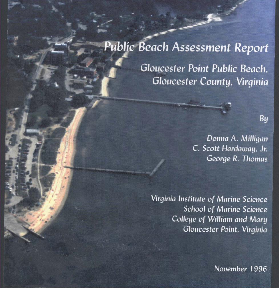
PUBLIC BEACH-ASSESSMENTREPORT

Gloucester Point Public Beach

Gloucester County, Virginia

by

Donna A. Milligan

C. Scott Hardaway, Jr.

George R. Thomas

Virginia Institute of Marine ScienceCollege of William and Mary

Gloucester Point, Virginia 23062

A Technical Report Obtained UnderContract with

The Virginia Department ofConservation and Recreation

for

The Board on Conservation and Developmentof Public Beaches

November 1996

-- - - -- - - - --

--- ---- --- -- --- ---

EXECUTIVE SUMMARY

Gloucester Point Public Beach is located at the southern end of Gloucester

County, Virginia on the York River. It is a southeastward facing sh<?reline about 960ft long and it is part of a larger stretch of moderately low shore between Sarah Creekand the George P. Coleman Bridge. While no s!,oreline improvement projects havetaken place at the public beach, shore protection projects updrift and including theVirginia Institute of Marine Science (VIMS) affect it. In 1983, erosion along theshoreline at VIMS just updrift of the public beach led to the installation of a ripraprevetment in front the seawall and the placement of 10,000 cubic yards (cy) of sand.A severe northeaster in November 1985 damaged the public beach and its facilities.Sand had to be bulldozed from the upland region at the public beach. In addition, anartificial dune was shaped, fenced, and planted. 500 cy of sand was placed at theVIMS. The Coleman Bridge widening project has greatly influenced the shoreline.The old boat ramp, located directly under the bridge, became inaccessible so a newboat ramp was constructed closer to the public beach where it has acted as a groin.

The purpose of this report is to assess the rates and patterns of change at thepublic beach. Field survey data, aerial photos, wave climate analysis and computermodeling were analyzed for this report. RCPW AVE, a wave hydrodynamic modeldeveloped by the US Army Corps of Engineers and modified by VIMS was used tomodel wave patterns.

In general, the littoral transport system moves sand south from updriftproperties to the public beach. The sand moves through the public beach southwardto the Point. The net long-term change along the public beach shoreline is erosion.However, change is variable along individual stretches of the shoreline. A slightembayment between the VIMS revetment and the public pier has developed and isevolving into a state of dynamic equilibrium. There has been little overall change inthe region where the orientation of the beach changes at the Point; this is a transitionarea where the littoral transport system is very active. Sand is accreting against thepublic boat ramp at Profile 54 and is being lost into the York River channel. Betweenthe boat ramp and the Coleman Bridge abutment, the shoreline is eroding due toconstruction and elimination of the sand supply.

With the reduction in sand supply due to shoreline hardening, it is importantto maintain and enhance the public beach's present planform. To achieve this, a spurat the VIMS/Gloucester Point beach boundary and one at the boat ramp arerecommended. In addition, a low reef breakwater should be placed at the public pier.Plans are already underway to construct a bulkhead between the boat ramp and theColeman Bridge abutment to abate erosion there.

i

TABLE OF CONTENTS

EXECUTIVESUMMARY I

TABLE OF CONTENTS - ii-

UST OF FIGURES.. . . . . . . . . . . . . . . . . . . . . . . . . . . . . . . . . . . . . . . . . . . . . . .. iv

UST OF TABLES . . . . . . . . . . . . . . . . . . . . . . . . . . . . . . . . . . . . . . . . . . . . . . . . . .. v

I. Introduction . . . . . . . . . . . . . . . . . . . . . . . . . . . . . . . . . . . . . . . . . . . . . . . . .. 1

A. Backgroundand Purpose . . . . . . . . . . . . . . . . . . . . . . . . . . . . . . . . . . . . .. 1B. Limitsof the StudyArea . . . . . . . . . . . . . . . . . . . . . . . . . . . . . . . . . . . . . . 4C. Approachand Methodology.. . . . . . . . . . . . . . . . . . . . . . . . . . . . . . . . . . 4

II. Coastal Setting . . . . . . . . . . . . . . . . . . . . . . . . . . . . . . . . . . . . . . . . . . . . . .. 10

A. Hydrodynamic Processes . . . . . . . . . . . . . . . . . . . . . . . . . . . . . . . . . . . .. 10

1. Wave Climate . . . . . . . . . . . . . . . . . . . . . . . . . . . . . . . . . . . . . . . . 102. Tides . . . . . . . . . . . . . . . . . . . . . . . . . . . . . . . . . . . . . . . . . . . . . . . 10

3. Stonn Surge 10

B. PhysicalSetting . . . . . . . . . . . . . . . . . . . . . . . . . . . . . . . . . . . . . . . . . . . . 10

1. Sediments 10

2. Shore Morphology 133. Sediment Transport 16

III. RCPWAVE. . . . . . . . . . . . . . . . . . . . . . . . . . . . . . . . . . . . . . . . . . . . . . . . . . 17

IV. Beach Characteristics 25

A. Beach Profiles and their Variabili ty . . . . . . . . . . . . . . . . . . . . . . . . . . . . . 25

B. Variability in ShorelinePosition . . . . . . . . . . . . . . . . . . . . . . . . . . . . . . . 32

C. Beach and Nearshore Volume Changes . . . . . . . . . . . . . . . . . . . . . . . . . . 34

ii

v. Summary and Conclusions . . . . . . . . . . . . . . . . . . . . . . . . . . . . . . . . . . . . . . 38

VI. Reco"mmendations. . . . . . . . . . . . . . . . . . . . . . . . . . . . . . . . . . . . . . . . . . . . 39

VI. References. . . . . . . . . . . . . . . . . . . . . . . . . . . . . . . . . . . . . . . . . . . . . . . . . . . 40

Appendix I. Gloucester Point Public Beach Sediment Data

Appendix II. Additional References about Uttoral Processes and

Hydrodynamic Modeling

Appendix III. Gloucester Point Public Beach Profiles

Hi

- ---------

LIST OF FIGURES

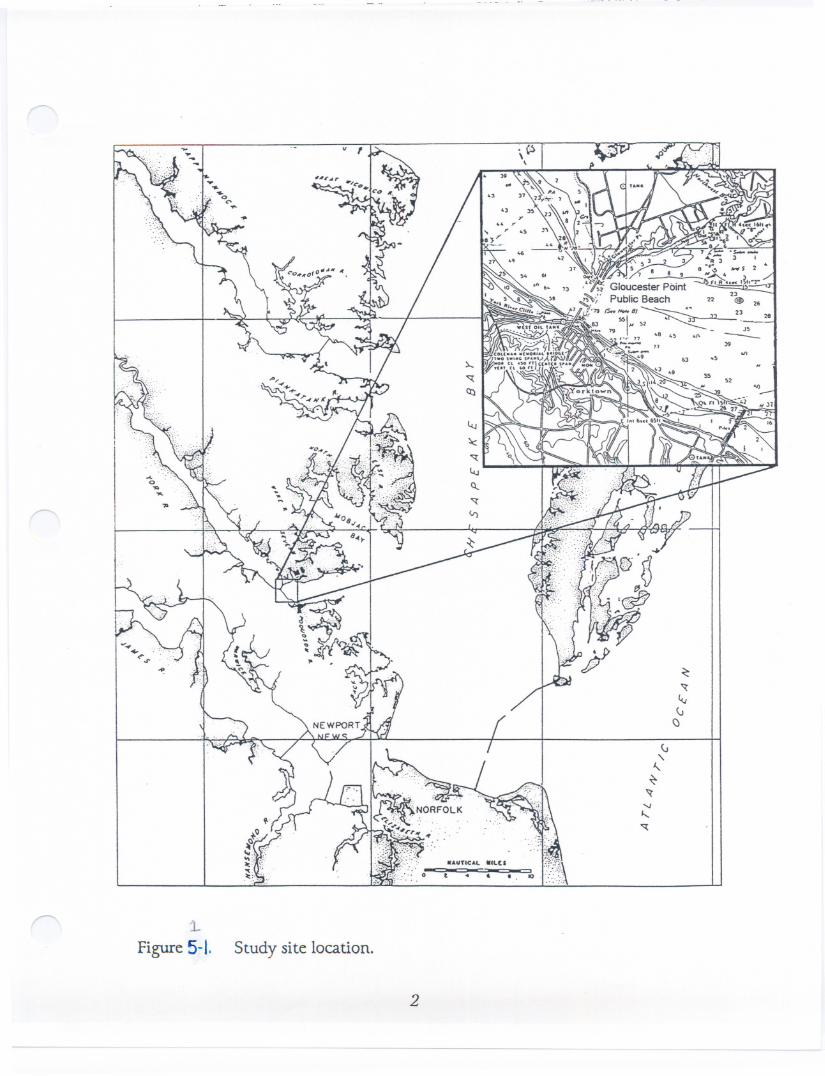
Figure 1. Study site location 2

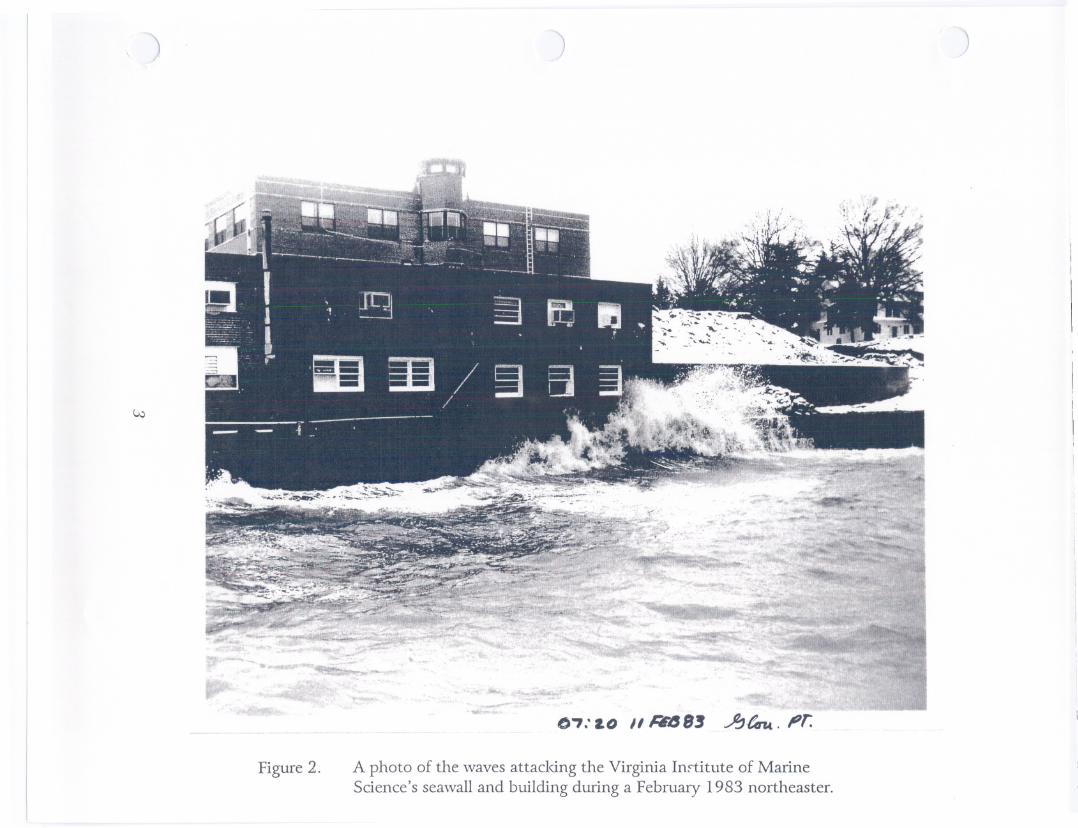
Figure 2. A photo of the waves attacking the Virginia Institute of MarineScience's seawall and building duri~g a February 1983 northeaster. . . 3

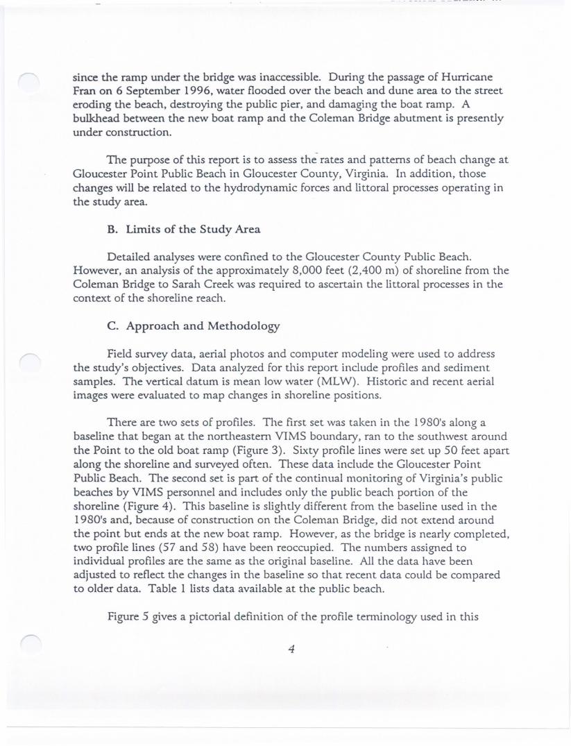
Figure 3. Basemap of Virginia Institute of Marine Science and Gloucester PointPublic Beach profile locations . . . . . . . . . . . . . . . . . . . . . . . . . . . . . . . . 5

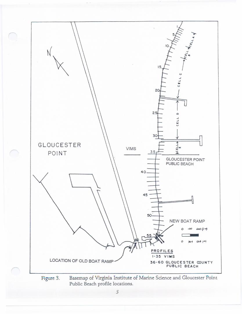
Figure4. Basemapof GloucesterPoint Beachwith profile locations. . . . . . . . . . 6

Figure 5. Beach profile demonstrating terminology used in the report 7

Figure a. Results of sediment analysis for mean grain size 12

Figure 6B. Results of sediment analysis for sorting 12

Figure 7. Aerial photos showing Gloucester Point shoreline in 1937, 1951,1968,and 1990 14

Figure 8A. Shoreline change between Sarah Creek and the point with percent ofprotected shoreline . . . . . . . . . . . . . . . . . . . . . . . . . . . . . . . . . . . . . . . 15

Figure 8B. 1992 color-coded shoreline showing type of shoreline and structuresbetween Sarah Creek and the Point . . . . . . . . . . . . . . . . . . . . . . . . . . 15

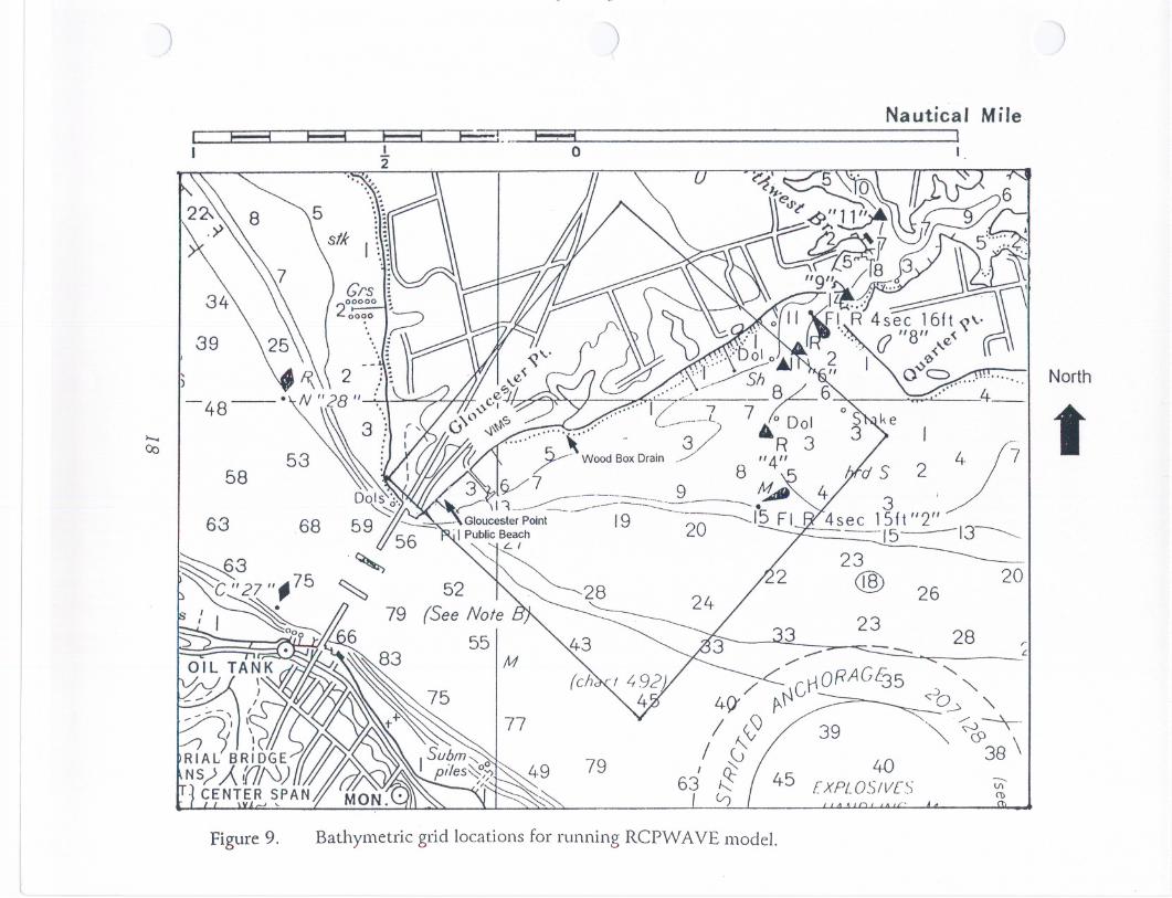
Figure 9. Bathymetric grid locations for nmning RCPWAVE model . . . . . . . .. 18

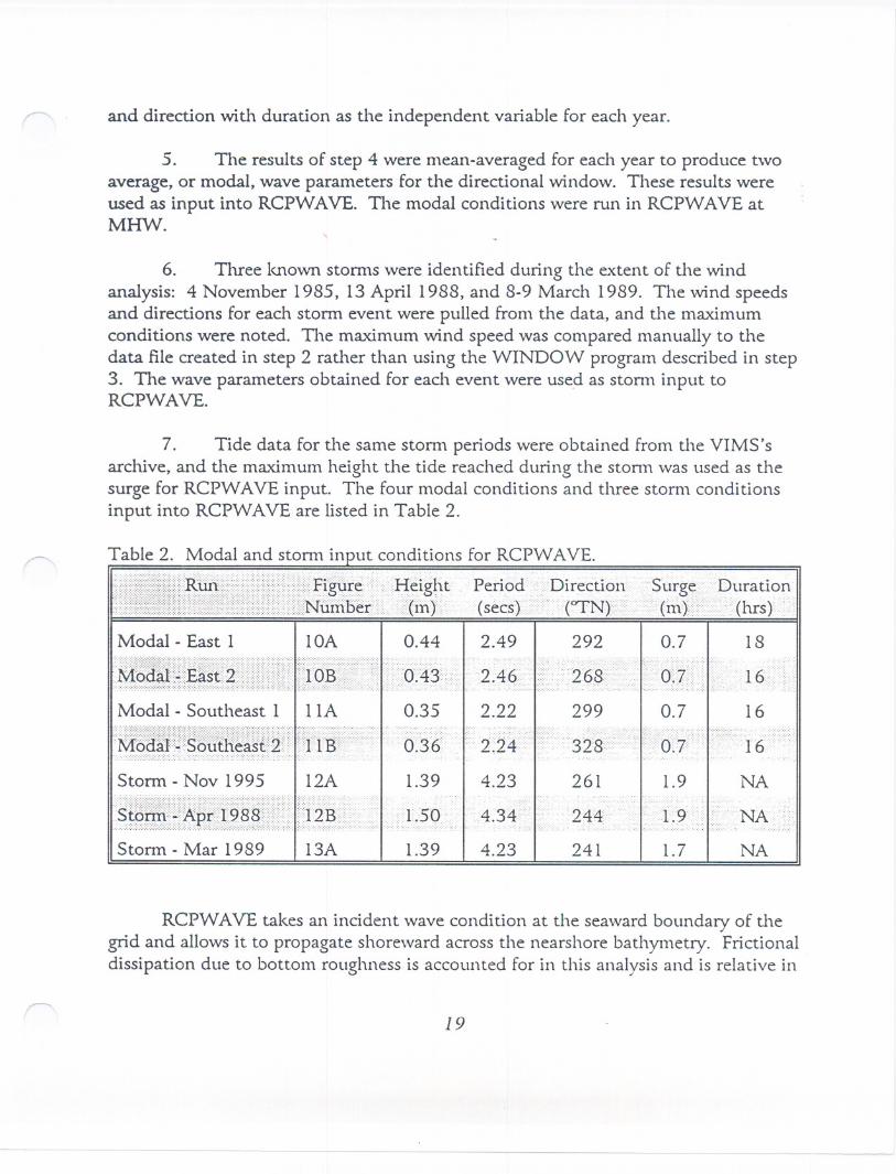
Figure lOA. Wave vector plots for modal conditions created from easterly windsand run at MHW . . . . . . . . . . . . . . . . . . . . . . . . . . . . . . . . . . . . . . . . 20

Figure lOB. Wave vector plots for modal conditions created from easterly windsand run at MHW . . . . . . . . . . . . . . . . . . . . . . . . . . . . . . . . . . . . . . . . 20

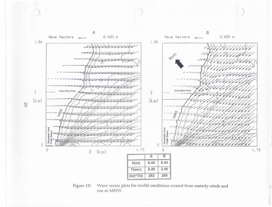
Figure liA. Wave vector plots for modal conditions created from southeasterlywinds and run at MHW . . . . . . . . . . . . . . . . . . . . . . . . . . . . . . . . . . . 21

Figure II B. Wave vector plots for modal conditions created from southeasterlywinds and run at MHW 21

iv

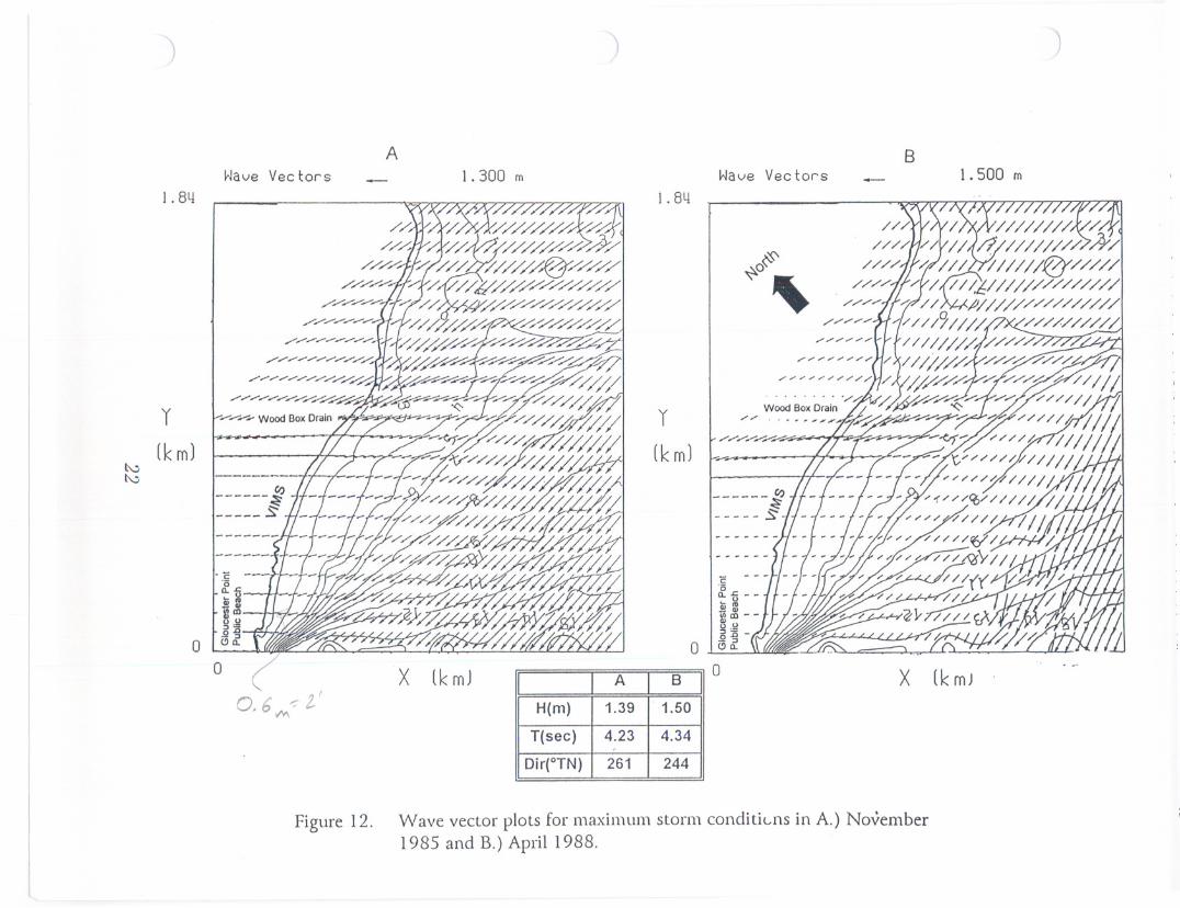
Figure 12A. Wave vector plots for maximum November 1985 storm conditions . 22

Figure 12B. Wave vector plots for maximum April 1988 storm conditions. . . . . . 22

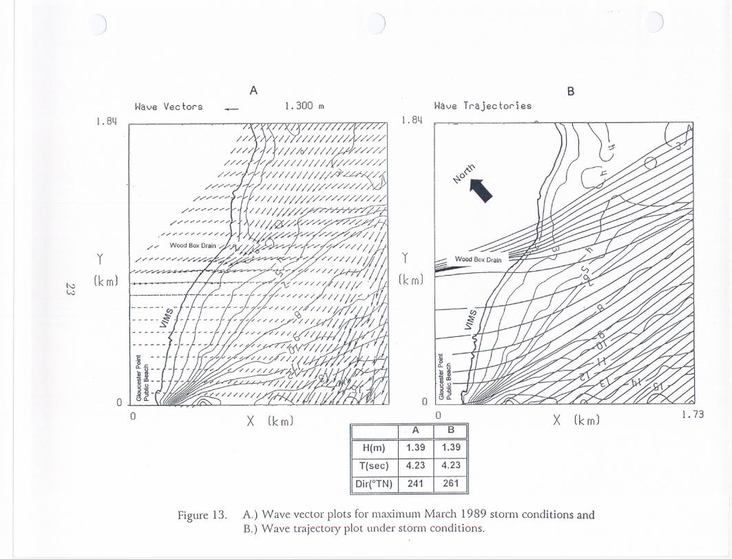
Figure 13A. Wave vector plots for maximum March 1989 storm conditions 23

Figure 13B. Wave trajectory plot under storm conditions. . . . . . . . . . . . . . . . . . . 23

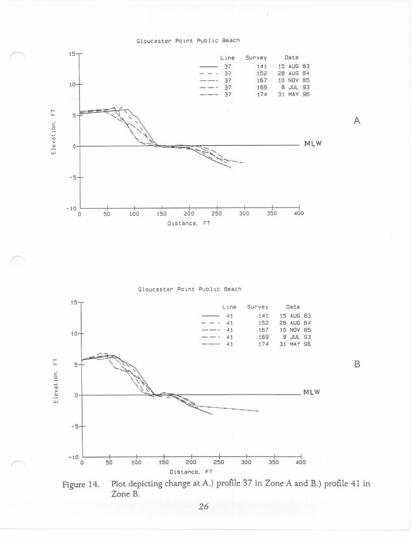
Figure 14A. Plot depicting change at profile 37 in Zone A 26

Figure 14B. Plot depicting change at profile 41 in Zone B 26

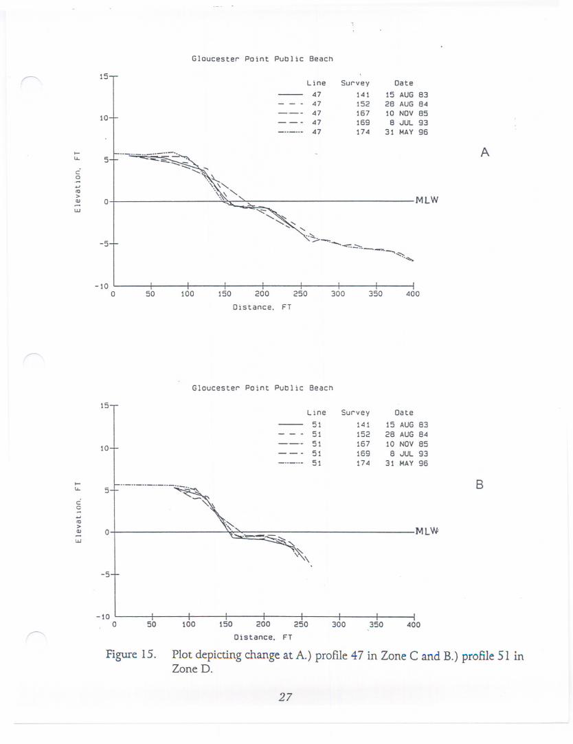
Figure 15A. Plot depicting change at profile 47 in Zone C 27

Figure 15B. Plot depicting change at profile 51 in Zone D 27

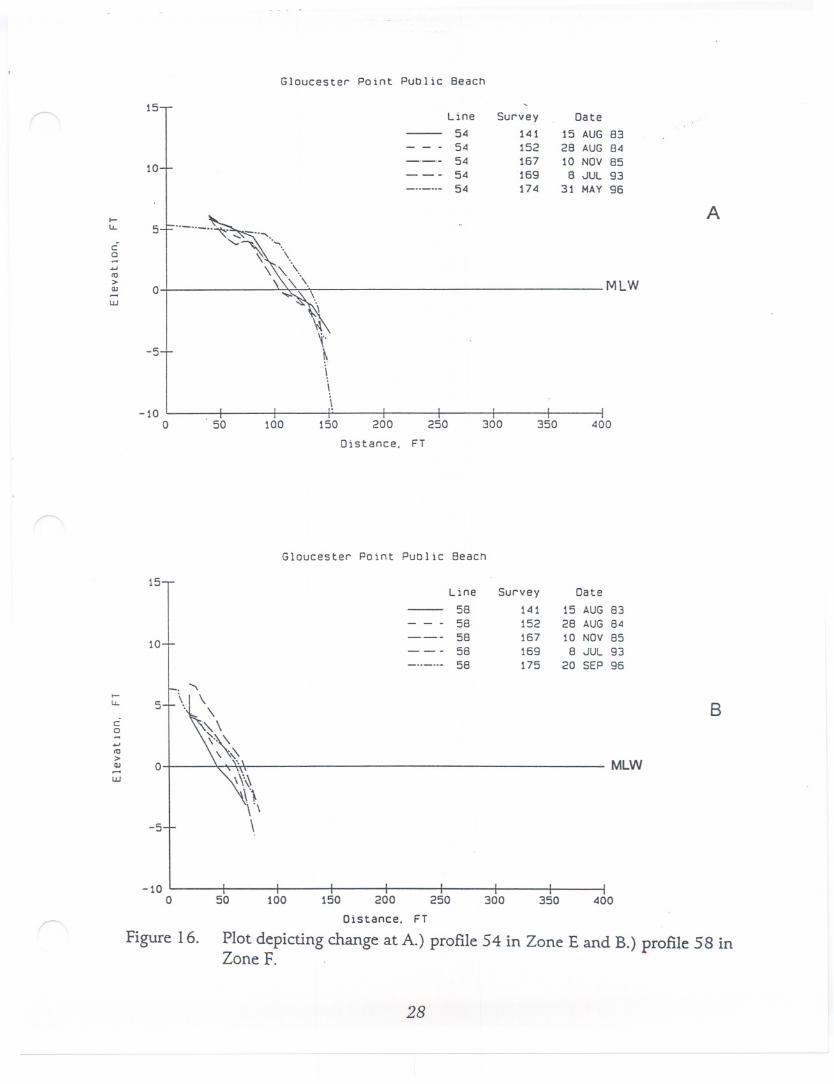
Figure 16A. Plot depicting change at profile 54 in Zone E 28

Figure 16B. Plot depicting change at profile 58 in Zone F . . . . . . . . . . . . . . . . . . . 28

Figure 17. Profile envelopes showing the envelope of change along thesoutheasterly facing shoreline . . . . . . . . . . . . . . . . . . . . . . . . . . . . . . . 30

Figure 18. Profile envelopes showing the envelope of change along theshoreline facing Yorktown next to the Coleman Bridge abutment .. . 31

Figure 19A. Distance of MHW from the baseline for profiles 36 through 54 33

Figure 19B. Distance of MHW from the baseline for profiles 57 and 58 33

Figure 20A. Volume change between sUlvey dates for the subaerial and nearshoreregions at profiles 36 through 54 . . . . . . . . . . . 35

Figure 20B. Volume change between survey dates for the subaerial and nearshoreregions at profiles 57 and 58 35

Figure 21. Total volume of the subaerial beach between profiles 36 and 54 overtime 37

v

Table 1.

Table 2.

LIST OF TABLES

List of available profile data along the Virginia Institute of MarineScience shoreline and Gloucester Point Public Beach . . . . . . . . . . . . . . 9

Wave conditions used as input to ~CPWAVE 19

vi

I. INTRODUCTION

A. Background and Purpose

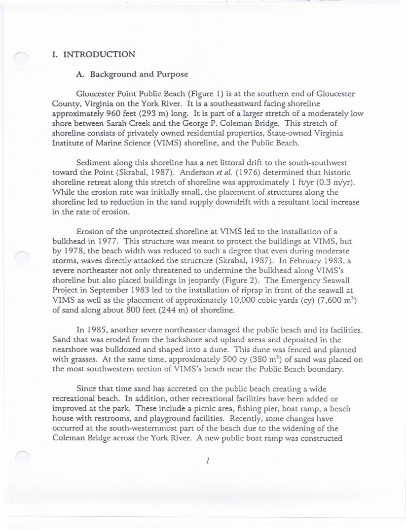
Gloucester Point Public Beach (Figure 1) is at the southern end of GloucesterCounty, Virginia on the York River. It is a southeastward facing shorelineapproximately 960 feet (293 m) long. It is part-of a larger stretch of a moderately lowshore between Sarah Creek and the George P. Coleman Bridge. This stretch ofshoreline consists of privately owned residential properties, State-owned VirginiaInstitute of Marine Science (VIMS) shoreline, and the Public Beach.

Sediment along this shoreline has a net littoral drift to the south-southwesttoward the Point (Skrabal, 1987). Anderson et al. (1976) determined that historic

shoreline retreat along this stretch of shoreline was approximately 1 ft/yr (0.3 m/yr).While the erosion rate was initially small, the placement of structures along theshoreline led to reduction in the sand supply downdrift with a resultant local increasein the rate of erosion.

Erosion of the unprotected shoreline at VIMS led to the installation of abulkhead in 1977. This structure was meant to protect the buildings at VIMS, butby 1978, the beach width was reduced to such a degree that even during moderatestorms, waves directly attacked the structure (Skrabal, 1987). In February 1983, asevere northeaster not only threatened to undermine the bulkhead along VIMS'sshoreline but also placed buildings in jeopardy (Figure 2). The Emergency SeawallProject in September 1983 led to the installation of riprap in front of the seawall atVIMS as well as the placement of approximately 10,000 cubic yards (cy) (7,600 m3)of sand along about 800 feet (244 m) of shoreline.

In 1985, another severe northeaster damaged the public beach and its facilities.Sand that was eroded from tl1e backshore and upland areas and deposited in thenearshore was bulldozed and shaped into a dune. This dune was fenced and plantedwith grasses. At the same time, approximately 500 cy (380 m3) of sand was placed onthe most southwestern section of VIlvlS's beach near the Public Beach boundary.

Since that time sand has accreted on the public beach creating a widerecreational beach. In addition, other recreational facilities have been added or

improved at the park. These include a picnic area, fishing pier, boat ramp, a beachhouse with restrooms, and playground facilities. Recently, some changes haveoccurred at the south-westernmost part of the beach due to the widening of theColeman Bridge across tl1e York River. A new public boat ramp was constructed

1

1-

Figure 5-1. Study site location.

2

w

)

J

.. ...~-

"" "'

I

IJ

o~.. &0 "RFlJ8! .h~. pr.

Figure 2. A photo of the waves attacldng the Virginia Inftitute of MarineScience's seawall and building during a February 1983 northeaster.

since the ramp under the bridge was inaccessible. During the passage of HurricaneFran on 6 September 1996, water flooded over the beach and dune area to the streeteroding the beach, destroying the public pier, and damaging the boat ramp. Abulkhead between the new boat ramp and the Coleman Bridge abutment is presentlyunder construction.

The purpose of this report is to assess the rates and patterns of beach change atGloucester Point Public Beach in Gloucester County, Virginia. In addition, thosechanges will be related to the hydrodynamic forces and littoral processes operating inthe study area.

B. Limits of the Study Area

Detailed analyses were confined to the Gloucester County Public Beach.However, an analysis of the approximately 8,000 feet (2,400 m) of shoreline from theColeman Bridge to Sarah Creek was required to ascertain the littoral processes in thecontext of the shoreline reach.

c. Approach and Methodology

Field survey data, aerial photos and computer modeling were used to addressthe study's objectives. Data analyzed for this report include profiles and sedimentsamples. The vertical datum is mean low water (MLW). Historic and recent aerialimages were evaluated to map changes in shoreline positions.

There are two sets of profiles. The first set was taken in the 1980's along abaseline that began at the nortl1eastern VIMS boundary, ran to the southwest aroundthe Point to the old boat ramp (Figure 3). Sixty profile lines were set up 50 feet apartalong the shoreline and surveyed often. These data include the Gloucester PointPublic Beach. The second set is part of the continual monitoring of Virginia's publicbeaches by VIMS personnel and includes only the public beach portion of theshoreline (Figure 4). This baseline is slightly different from the baseline used in the1980's and, because of construction on the Coleman Bridge, did not extend aroundthe point but ends at the new boat ramp. However, as the bridge is nearly completed,two profile lines (57 and 58) have been reoccupied. The numbers assigned toindividual profiles are the same as the original baseline. All the data have beenadjusted to reflect the changes in the baseline so that recent data could be comparedto older data. Table I lists data available at the public beach.

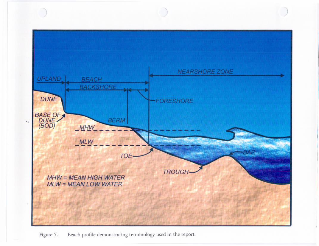
Figure 5 gives a pictorial definition of the profile terminology used in this

4

GLOUCESTERPOINT

VIMS

u..J..JWU

GLOUCESTER POINTPUBLIC BEACH

40

45

o .00 Leo (r~

LOCATION OF OLD BOAT RAMP

PROFILES

1-35 VIMS

36-60 GLOUCESTER COUNTYPUBLIC BEACH

Figure 3. Basemapof Virginia Institute ofMarine Scienceand GloucesterPointPublic Beach profile locations.

5

2......-. C

..J

..I

..U

I3

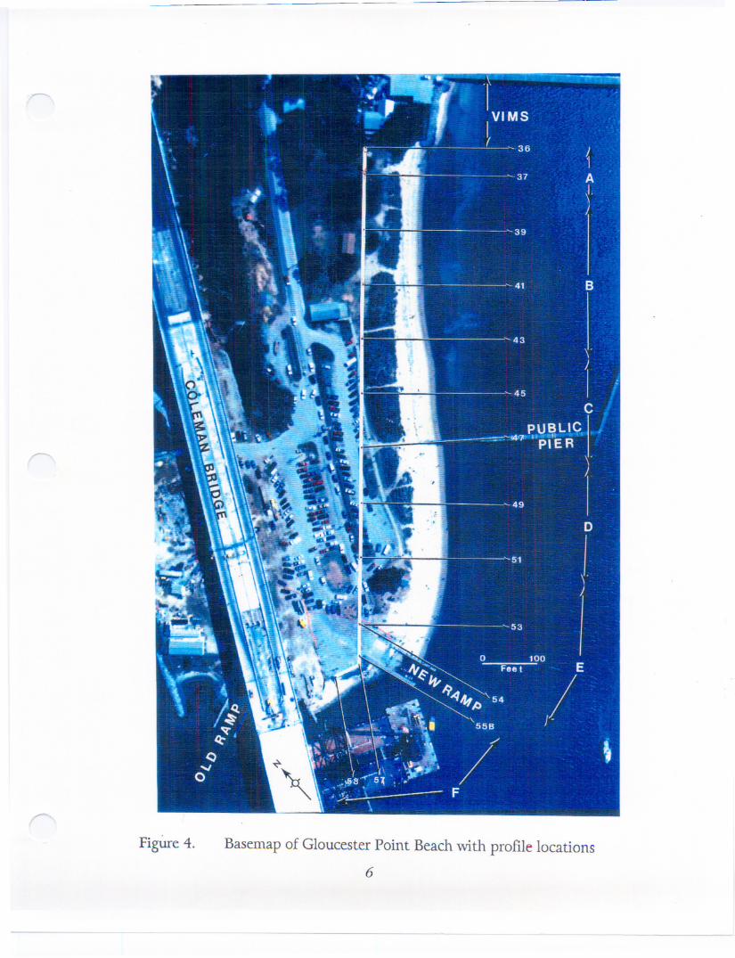
FigUre4. Basemap of Gloucester Point Beach with profile locations

6

BASEO~'J I DUNE(BOD) _"d.HJ!V__ _ _ _ _

MLW

TOE

MHW = MEAN HIGH WATERMLW = MEAN LOW WATER

Figure 5. Beach profile demonstrating terminology used in the report.

- ---- _. -- -. +--. .. - - . ------------

report. Nearshore volume calculations take into account all the sand below MLW tothe end of each profile. The subaerial beach occurs above MLW and is divided intothe beach face (foreshore) and backshore regions.

The hydrodynamic forces acting along the Gloucester Point shore reach wereevaluated using RCPW AVE, a computer model developed by the U.S. Army Corps ofEngineers (Ebersole et al., 1986). RCPWA VE is a linear wave propagation modeldesigned for engineering applications. This model computes changes in wavecharacteristics that result naturally from refraction, shoaling, and diffraction overcomplex shoreface topography. To this fundamental linear-theory based model,oceanographers at VIMS have added routines which employ recently developedunderstandings of wave bottom boundary layers to estimate wave energy dissipationdue to bottom friction. The reader is referred to Ebersole et al. (1986) and Wright etale (1987) for a thorough discussion of RCPW AVE, its use, and theory.

The model was run using modal and storm incident wave conditions (waveheight, period, and direction) which were detennined following procedures outlinedby the U.S. Army Corps of Engineers' Shore Protection Manual (1977 and 1984).These procedures are based on wincl/wave hindcast methods across fetch-limitedwater bodies which were developed by Sverdntp and Monk (1947) and revised byBretshneider (1952, 1958). The 5MB model used in this study was further modifiedby IGley (1982) and is essentially a shallow water, estuarine, wind-wave predictionmodel. Wind data, obtained from Virginia Power's Yorktown Station which is 2.7nm (5 km) southeast of Gloucester Point Beach, were used to develop the incidentwave conditions for input to the RCPW AVE program.

8

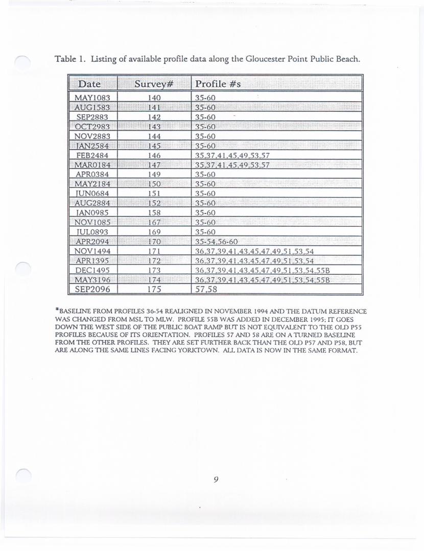
Table 1. Listing of available profile data along the Gloucester Point Public Beach.

....., H. ._ ""..,h .. .

li:::::i:::::~:~t~:::::::::::::::::::::.::::::::::::::.:::::.:::::$Urv~v~.:.:...::.:..:.':..:I.:..Pr6file:#s:

MAYI083 I 140 ~-60!:::::AUG:-j:l5:Sg::::(::

SEP28831{:::OCT29S@:/:::=

NOV2883. ... ... ...

(::::::tA:N2SB'4::::::(:FEB2484

':::::MARdil}4::::::::APR0384

../MAY2ls4t:)UN0684

::t.xU02Sg4::::tAN0985

.::NOVIOg:S:::.UL0893

}:6APR209'4):J?NOV1494

}/APR1395:tfDEC1495

.::MAY3t9:&/SEP2096

173

35-60. .. .

"35~6m: ....

35.37.41.45.49.53.57.. .. . . . .

..35;:3:7\'41,45;49';'5357

35-60

. 35~60:"

35-60;35~60::{

35-60

. 35~60..35-60

35~54.56~60

36,37.39.41.43.45.47.49.51.53.5436.37.39,41.43.45.47.49~5 L53.5436.37.39.41.43.45.47.49.51.53.54.55B

. .

36.37:;39.41.43; 45.4'7.49'!5t=~53T54;;55B.57.58175

*BASEUNE FROM PROFILES 36-54 REALIGNED IN NOVEMBER 1994 AND THE DA11.1MREFERENCEWAS CHANGED FROM MSL TO MLW. PROFILE 55B WAS ADDED IN DECEMBER 1995; IT GOESDOWN THE WEST SIDE OF THE PUBUC BOAT RAMP Bur IS NOT EQUIVALENTTO THE OLD P55PROFILES BECAUSE OF ITS ORIENTATION. PROFILES 57 AND 58 ARE ON A l1JRNED BASEUNEFROM THE OTHER PROFILES. THEY ARE SET FURTHER BACKTHAN THE OLD P57 AND P58. BUTARE ALONG THE SAME UNES FACING YORIcrOWN. ALLDATA IS NOW IN THE SAME FORMAT.

9

...-... . ..- - ... -- .. . - . - - .. . -. - - - -- - .. - -.. . - - ... - - . .- - - --

II. COASTAL SETTING

A. Hydrodynamic Processes

1. Wave Climate.-

The wave climate at Gloucester Point beach is affected by waves generatedboth locally and within the Chesapeake Bay as well as by nearshore bathYmetry, tidalcurrents, and freshwater flow. The public beach is e..xposedto westward travelingwaves since it faces the mouth of the York River. The shoreline is orientated

approximately N52°E and has an average fetch to the southeast across the York Riverand Chesapealce Bay of 12.6 miles (20.24 km) (Skrabal, 1987). Its ma.ximum fetch is29 miles (46 km) to the east. The nearshore region is influenced by the York Riverchannel that runs close to the shoreline. The York River channel e..xperiences heavyuse by commercial and military ships whose wakes minimally affect the overall waveclimate at Gloucester Point.

2. Tides

The mean tidal range at Gloucester Point Beach is 2.4 ft (73 cm) with a springrange of 2.8 ft (85 cm)(Tidelog, 1996).

3. Storm Surge

Boon et al. (1978) statistically determined storm surge frequency for bothe..xtratropicaland tropical storm events. In the Gloucester Point area, the storm surgelevels for 10 year, 50 year, and 100 year events are 5.8 ft (1.8 m), 6.6 ft (2.0 m), and7.1 ft (2.2 m), respectively. These surge levels are heights above MLW. The Corpsof Engineers (U.S. Army Corps of Engineers, 1993) reports higher values for the samestorm frequencies. These storn1 surge levels for 10 year, 50 year, and 100 year eventsare 7.6 ft (2.3 m), 9.0 ft (2.7 m), and 9.7 ft (3.0 m), respectively.

B. Physical Setting

1. Sediments

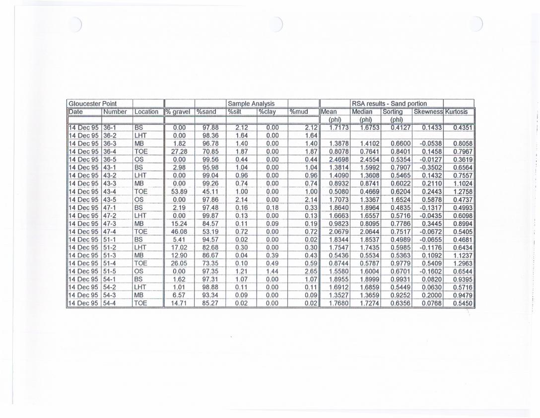
In general, the sediments at Gloucester Point beach consist of sand with somegravel. The silt and clay content in the samples is less than five percent and will bedisregarded in this analysis. Additional sediment data are available in Appendix I.

10

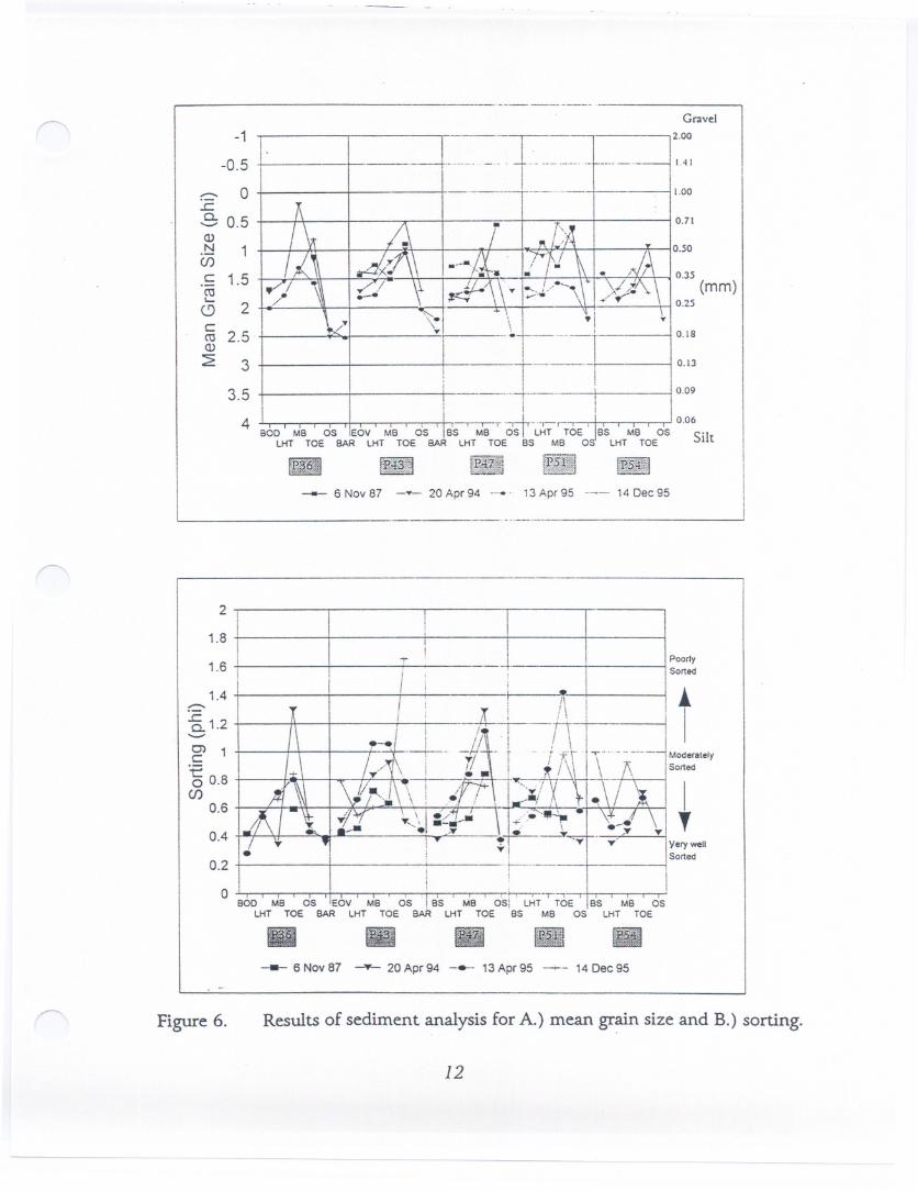
Sediment samples were taken along 5 profile lines; these profiles are 36,43,47,51 and 54. Certain morphologic points were sampled consistently from date todate. The base of dune (BOD), edge of vegetation (EOV) and backshore (BS)samples represent the area of the beach that is influenced by eolian transport andrun-up from occasional storm events. Sediments were also taken at last high tide(LHT), midbeach (MB), toe, and offshore (OS). The toe of the beach is located atthe breal, in slope between the beach face and the nearshore region. It is sometimesevidenced by a distinct change in sediment type. See Figure 5 for definition of terms.

The grain size distribution of beach sand generally varies across shore and, to alesser degree, alongshore as a function of tl1e mode of deposition. The coarsest sandparticles usually are found where the backwash meets the incoming swash in a zone ofmaximum turbulence at the base of the subaerial beach; here the sand is abruptlydeposited creating a step or toe. Just offshore, the sand becomes finer. Another areaof coarse particle accumulation is the berm crest, which is sometimes coincident withLHT, where run up deposits all grain sizes as the swash momentarily stops before thebacl<:wash starts. The dune or backshore generally contains the finest particlesbecause deposition here is limited by the wind's ability to entrain and move sand(Bascom, 1959; Stauble et al., 1993). This is typical of estuarine beaches in theChesapeake Bay (Hardaway et aI., 1991 ).

The sorting of sediments can be described by the Inclusive Graphic StandardDeviation (Folk, 1980). The spread of the grain size distribution about the meandefines the concept of sorting. Well sorted sands will have a frequency distributioncurve that is sharp peaked and narrow; this means only a few size classes are present(Friedman and Sanders, 1978). Poorly sorted sediments are represented by most sizeclasses in the sample.

Figures a and B are plots of mean grain size and sorting of the sand portion ofthe sample for 5 profiles. Several trends are obvious in Figure a. The wide variabilityin grain size along the beach indicate an active littoral system at Gloucester Point.There is no consistent trend in grain size along the beach only across each profile.Midbeach and toe are consistently the coarsest material along the beach while theoffshore samples are the finest. In general, this beach follows the typical model ofgrain size along a profile line. Overall, sand size distribution is finer at tl1e base ofdune and backshore and in the nearshore and coarser along the beach berm (LHT),midbeach and toe. Profile 51 had the widest distribution of grain size whichindicates sand is being transported through this profile.

Figure 6B shows the sorting of each sample. In general, profile 36 is somewhat

11

.

Gravel

2.00

. . , -.-. 1.41

1.00

0.71

o.so

0.18

r----, i

I I

BOD MB OS IEOV MB OS' Ia's~ ost-~;':-' TOE'LHT TOE BAR LHT TOE BAR LHT TOE BS MB 0

0.13

0.09

. . .. 0.06BSMBOS.

LHT TOE SlIt

- 6 Nov 87 -- 20 Apr 94 --. - 13 Apr 95 --- 14 Dee 95

Figure 6.

o BOD' MB ' o'S 'IEOV' MB ' OS ! as MB' o's! uIT-oTOE IBS MB OSLHT TOE BAR LHT TOE BAR LHT TOE BS MB OS LHT TOE

--- 6 Nov87 ---'tI'-20 Apr94 -- 13Apr95 --+-- 14Dee95

Results of sediment analysis for A.) mean grain size and B.) sorting.

12

-1

-0.5

......... a

.cS 0.5Q)N 1U55 1.5cu'-

2<.9c::cu 2.5Q)

3

3.5

4

2

1.8

I

i II I POOrly1.6

-r-+ Sorted

1.4 I

t:=-.c0.. 1.2.........C) 1 Moderatelyc::

Sortedt

I

00.8en

0.6

'I'!-0.4,-

..... .Y-r---"'. y'

,YITi

y! . Sorted0.2

. ..- - ... .-- ... . - ... .. . -- -- - -----

better sorted than profiles 43 and 47. These three sample profiles have a cross shoretrend that suggests the toe is the most poorly sorted samples and the base ofdune/backshore and nearshore samples are well sorted. Sorting across profile 51 isextremely variable indicating an active littoral zone. Profile 54 seems to be becomingmore poorly sorted through time except at the toe of the beach.

2. Shore Morphology

The shore morphology is determined by long-term impact of the impingingwave climate after the waves have been altered by the nearshore bathYffietry, tidalcurrents, and coastal structures. BYrne and Anderson (1977) found that between1868 and 1942 the shoreline from Sarah Creek to Wood Box Drain, the headland

located about halfway between Sarah Creek and the Point, was eroding at an averageof 0.9 ftlYf (0.3 m/Yf). The beach along this shore, with the exception of the publicbeach, is thin and narrow. The nearshore region is narrow near the point, reachingintermediate off Sarah Creek's entrance.

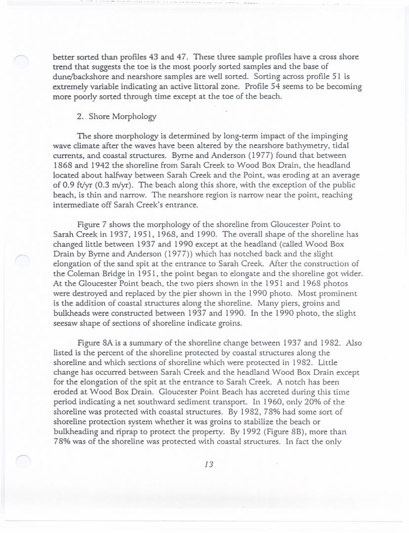
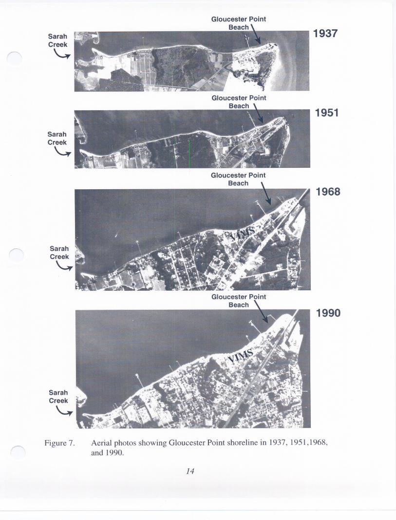
Figure 7 shows the morphology of the shoreline from Gloucester Point toSarah Creek in 1937, 1951, 1968, and 1990. The overall shape of the shoreline haschanged little between 1937 and 1990 except at the headland (called Wood BoxDrain by BYrne and Anderson (1977» which has notched back and the slightelongation of the sand spit at the entrance to Sarah Creek. Mter the construction ofthe Coleman Bridge in 1951, the point began to elongate and the shoreline got wider.At the Gloucester Point beach, the two piers shown in the 1951 and 1968 photoswere destroyed and replaced by the pier shown in the 1990 photo. Most prominentis the addition of coastal structures along the shoreline. Many piers, groins andbulkheads were constructed between 1937 and 1990. In the 1990 photo, the slightseesaw shape of sections of shoreline indicate groins.

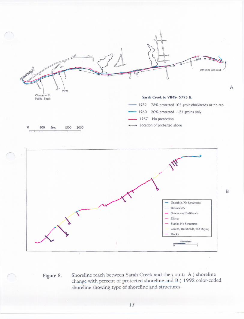
Figure 8A is a summary of the shoreline change between 1937 and 1982. Alsolisted is the percent of the shoreline protected by coastal structures along theshoreline and which sections of shoreline which were protected in 1982. Littlechange has occurred between Sarah Creek and the headland Wood Box Drain e..xceptfor the elongation of the spit at the entrance to Sarah Creek. A notch has beeneroded at Wood Box Drain. Gloucester Point Beach has accreted during this timeperiod indicating a net southward sediment transport. In 1960, only 20% of theshoreline was protected with coastal structures. By 1982, 78% had some sort ofshoreline protection system whether it was groins to stabilize the beach orbulkheading and riprap to protect the property. By 1992 (Figure 8B), more than78% was of the shoreline was protected with coastal structures. In fact the only

13

SarahCreek

~

SarahCreek

~

SarahCreek

~

SarahCreek

~

Figure7. Aerial photos showing Gloucester Point shoreline in 1937, 1951,1968,and 1990.

14

--- -

1937

1951

1968

1990

A

Gloucester Pt.Public Beach Sarah Creek to VIMS- 5775 ft.

o 500 Feet 1500 2000

- 1982 78%protected105groins/bulkheadsor rip-rap- 1960 20%protected-24 groinsonly

1937 No protection

_ locationof protectedshoreI I I I I I

'"

B

- Unstable,No Structures

BreakwaterGroins and Bulkheads

Riprap

Stable, No Structures

Groins, Bulkheads, and Riprap

Docks

kilometersII

-Figure8. Shoreline reach between Sarah Creek and the! oint: A.) shoreline

change with percent of protected shoreline and B.) 1992 color-codedshoreline showing type of shoreline and structures,

15

-- unprotected shoreline was the public beach, the headland at Wood Box Drain, thespit at the entrance to Sarah Creek, and one other small piece of shoreline.

3. Sediment Transport

The net southward component of littorartransport has been documented alongthe Gloucester Point shoreline. The accretion at the point demonstrates sandmovement. A component of littoral transport also probably moves sand riverwardand into the York River channel where it is lost to the system.

According to Anderson et al. (1976) this section of shoreline has a limited

amount of sand naturally available to maintain its beaches. Originally, sand erodedfrom upland areas supplied downdrift beaches. Sand was transported south along theshoreline to the public beach and around the Point where it stacked up against theColeman Bridge abutment or was lost to the York River channel. With the

proliferation of coastal protection structures, shoreline retreat has been stopped alongmany sections. However, if the sand supply to the littoral transport system iseliminated, the beaches along this shoreline may disappear if they are no longer ableto maintain themselves. This will place shore structures in jeopardy, and sand will nolonger be supplied to the public beach. This transport system was intemlpted in1994 with the construction of a new public boat ramp at Gloucester Point Beach.Sand is stacking against the boat ramp and being transported into the York Riverchannel, eliminating the sand supply to the point.

..--

16

------

-- ... --. . . - --. -.. . - ... ..--

III. RCPWAVE

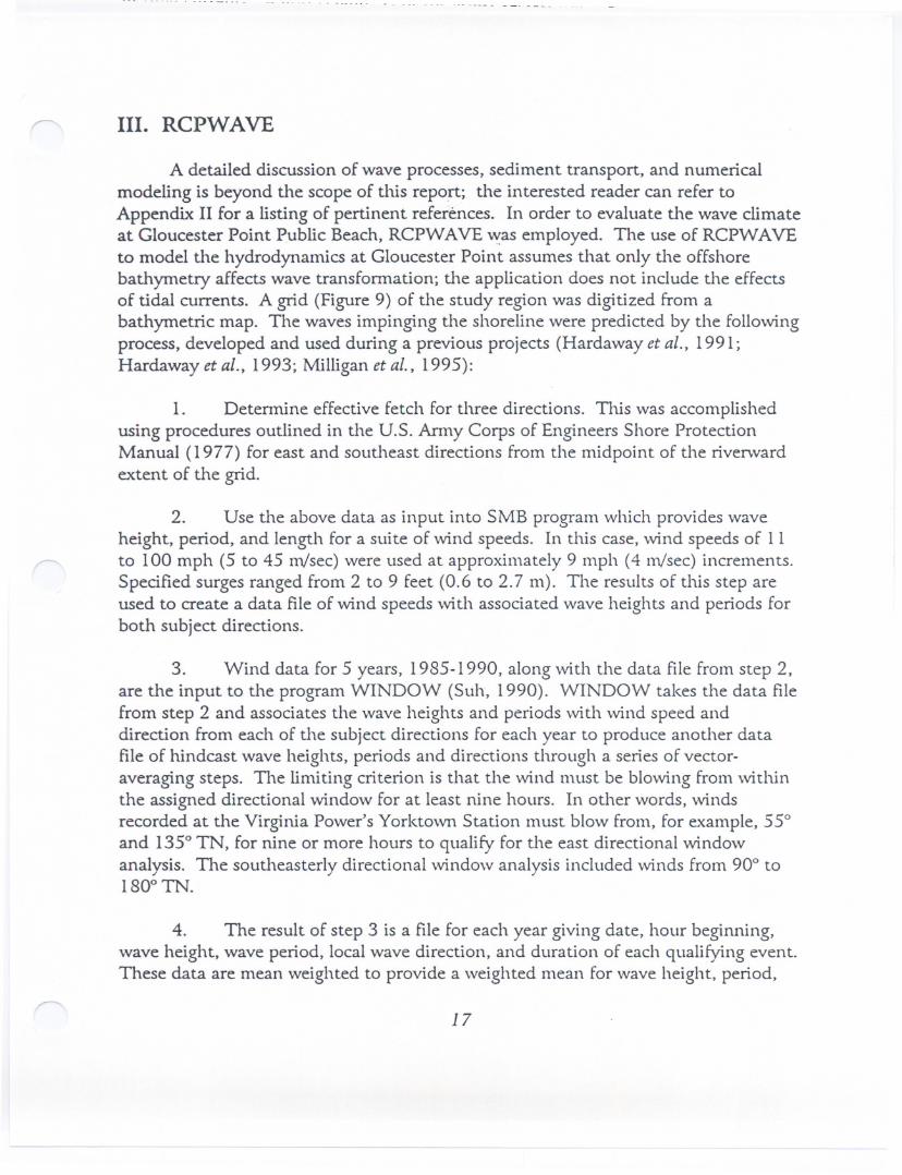
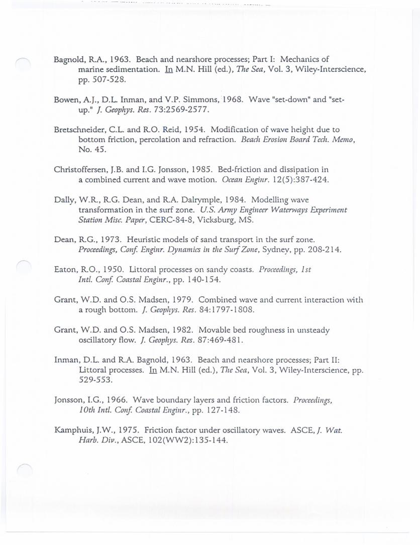
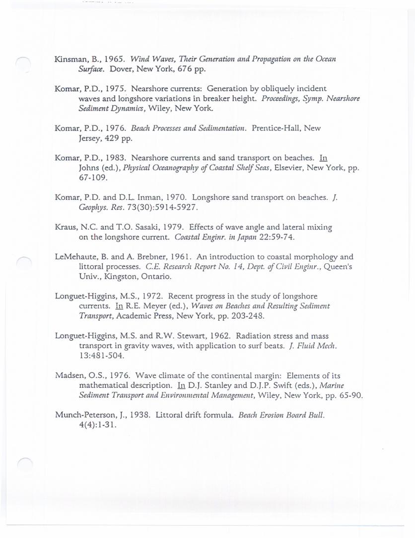
A detailed discussion of wave processes, sediment transport, and numericalmodeling is beyond the scope of this report; the interested reader can refer toAppendix II for a listing of pertinent references. In order to evaluate the wave climateat Gloucester Point Public Beach, RCPWAVE ~as employed. The use of RCPWAVEto model the hydrodynamics at Gloucester Point assumes that only the offshorebathYmetry affects wave transformation; the application does not include the effectsof tidal currents. A grid (Figure 9) of the study region was digitized from abathYmetric map. The waves impinging the shoreline were predicted by the followingprocess, developed and used during a previous projects (Hardaway et a/., 1991;Hardaway et al., 1993; Milligan et al., 1995):

1. Determine effective fetch for three directions. This was accomplishedusing procedures outlined in the U.S. Army Corps of Engineers Shore ProtectionManual (1977) for east and southeast directions from the midpoint of the rivenvardextent of the grid.

2. Use the above data as input into 5MB program which provides waveheight, period, and length for a suite of wind speeds. In this case, wind speeds of 11to 100 mph (5 to 45 m/sec) were used at approximately 9 mph (4 m/sec) increments.Specified surges ranged from 2 to 9 feet (0.6 to 2.7 m). The results of this step areused to create a data file of wind speeds with associated wave heights and periods forboth subject directions.

3. Wind data for 5 years, 1985-1990, along with the data file from step 2,are the input to the program WINDOW (Suh, 1990). WINDOW takes the data filefrom step 2 and associates the wave heights and periods with wind speed anddirection from each of the subject directions for each year to produce another datafile of hindcast wave heights, periods and directions through a series of vector-averaging steps. The limiting criterion is that the wind must be blowing from withinthe assigned directional window for at least nine hours. In other words, windsrecorded at the Virginia Power's Yorktown Station must blow from, for example, 550and 1350 TN, for nine or more hours to qualify for the east directional windowanalysis. The southeasterly directional window analysis included winds from 900 to1800 TN.

4. The result of step 3 is a file for each year giving date, hour beginning,wave height, wave period, local wave direction, and duration of each qualifying event.These data are mean weighted to provide a weighted mean for wave height, period,

17

) )

Nautical MileI 1---4 ~ ~ I---!_ ~ II ! 0 I

2 .

1-..0Q:)

")

58

63 .68

26

2328--

79

....-....

__ 00RAGtj5/ ...\C.49' ~\"

/ ~<v\)/ 39/ ()

/ 4063 § 45 [XPLOSIV£S

V)

"-

"b '"~ "-

"'" ~OJ-T-38 \-

VICb

Figure9. Bathymetric grid locations for running RCPW A VE model.

North

rt:.

and direction with duration as the independent variable for each year.

5. The results of step 4 were mean-averaged for each year to produce twoaverage, or modal, wave parameters for the directional window. These results wereused as input into RCPWAVE. The modal conditions were run in RCPWAVE atMHW.

6. Three known storms were identified during the extent of the windanalysis: 4 November 1985, 13 April 1988, and 8-9 March 1989. The wind speedsand directions for each storm event were pulled from the data, and the maximumconditions were noted. The maximum wind speed was compared manually to thedata file created in step 2 rather than using the WINDOW program described in step3. The wave parameters obtained for each event were use.d as storm input toRCPW AVE.

7. Tide data for the same storm periods were obtained from the VIMS'sarchive, and the maximum height the tide reached during the storm was used as thesurge for RCPWAVE input. The four modal conditions and three storm conditionsinput into RCPWAVE are listed in Table 2.

2.49 292 0.7 18

Storm - Mar 1989 13A

. .

2.46

2.22

2.24

4.23

4.34

4.23

Modal - Southeast 1.::".;.;.;.:.;.;.;.;.;.:.:.;.::::;.::;.;:;.::;:;.;:::;:::;:::;::::::::;::.:.:.:.:::::::-:::::::::(:.;::::.::.:.:.":.'.: .........................................................................................................................

..Nfba~t.5\S8tifii~£st2ni.....

Storm -Nov 1995" ..... . . . . .. - . . . . . . . . . . .. . ....... . . .. . . . . . . . . . . . . . . .. ......................... . . . .. . . .. .. . . .......... ...... . . . . . . . . .. . . . . .. . . . . . .. .. .....

sl8HHJ:wp..rUI988=:..:;.::;:::;:::::::::::::::::::::::::::::::::::::;::::::: ;::::::::;:;::::;;;:::::::::::::::::::::::::::::

1.39 241 1.7

.NA..

NA

RCPW AVE takes an incident wave condition at the seaward boundary of thegrid and allows it to propagate shoreward across the nearshore bathymetry. Frictionaldissipation due to bottom roughness is accounted for in this analysis and is relative in

19

-- - - ----

AWave Vectors 0.400 m-

1. 84

y

N (kmJc

c

~j.i~

o I C> Il.

o X (k m) I. 73

\

1. 84

y

(k mJ

BWave Vectors 0.400 m-

~~~o

~

c'0Il..t:

in ~ -----.

~~ ~- :>

o I C>Il.

o 1.73

Figure 10. Wave vector plots for modal conditions created from easterly winds andrun at MHW.

I I-A I BI

H(m) 0.44 0.43

T(sec) 2.49 2.46

Dir(OTN) 292 268

\. 84

N....

y

(km)

AWave Vectors 0.300 m-

- - ---

Wood Box Drain

c.0':gi~~~~cr

o J.73X (k m)

1.84

y

(k m)

Wave VectorsB

0.300 m-~o~'" ~

~ ~---'. ~

'--- :::::

" , ' ,~

"E

-&'5,~ ~!..

a~--::>-~Il.

o X (k m) 1.73

Figure 11. Wave vector plots for modal conditions created from southeasterlywinds and run at MHW.

I I

A I B IH(m) 0.35 0.36

T(sec) 2.22 2.24

Dir(OTN) 299 328

1. 84

'(

(k m)l'\,j~

o

AWave Vectors 1.300 m

(O. b ,. 2- I

>/VI

x

1.84

'(

(k m)

8Wave Vectors 1.500 m

~

"0,

X (kmJ

Figure 12. Wave vector plots for ma.ximumstorm conditiLns in A.) November1985 and B.) April 1988.

I I A I B IH(m) 1.39 1.50

T(sec) 4.23 4.34,

Dir(OTN) 261 244

I. 84

NW

'(

(k m)

AWave Vectors 1.300 m

oo

c - - -1-

H::~n_(!)~

x

1.84

'(

(k m)

c'0o..'fiIii m

~~:J==on

o I i3~o

)

BWave Trajectories

~'<:-

"0,

X (k m) 1.73

Figure 13. A.) Wave vector plots for maximum March 1989 storm conditions andB.) Wave trajectory plot under storm conditions.

I I A I B IH(m) 1.39 1.39

T(sec) 4.23 4.23

Dir(OTN) 241 261

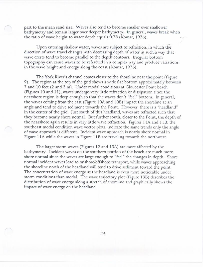
part to the mean sand size. Waves also tend to become smaller over shallowerbathymetry and remain larger over deeper bathymetry. In general, waves break whenthe ratio of wave height to water depth equals.0.78 (Komar, 1976).

. -Upon entering shallow water, waves are subject to refraction, in which the

direction of wave travel changes with decreasing depth of water in such a way thatwave crests tend to become parallel to the depth contours. Irregular bottomtopography can cause waves to be refracted in a complex way and produce variationsin the wave height and energy along the coast (Komar, 1976).

The York River's channel comes closer to the shoreline near the point (Figure9). The region at the top of the grid shows a wide flat bottom approximately between7 and 10 feet (2 and 3 m). Under modal conditions at Gloucester Point beach(Figures 10 and II), waves undergo very little refraction or dissipation since thenearshore region is deep enough so that the waves don't "feel" bottom. In general,the waves coming from the east (Figure lOA and lOB) impact the shoreline at anangle and tend to drive sediment towards the Point. However, there is a "headland"in the center of the grid. Just south of this headland, waves are refracted such thatthey become nearly shore normal. But further south, closer to the Point, the depth ofthe nearshore again results in very little wave refraction. Figures II A and II B, thesoutheast modal condition wave vector plots, indicate the same trends only the angleof wave approach is different. Incident wave approach is nearly shore nonnal inFigure IIA while the waves in Figure II B are traveling towards the northwest.

The larger storm waves (Figures 12 and 13A) are more affected by thebathymetry. Incident waves on the southen1 portion of the beach are much moreshore normal since the waves are large enough to "feel" the changes in depth. Shorenormal incident waves lead to onshore/offshore transport, while waves approachingthe shoreline north of the headland will tend to drive sediment toward the point.The concentration of wave energy at the headland is even more noticeable understorm conditions than modal. The wave trajectory plot (Figure 13B) describes thedistribution of wave energy along a stretch of shoreline and graphically shows theimpact of wave energy on the headland.

24

IV. BEACH CHARACTERISTICS

A. Beach Profiles and their Variability

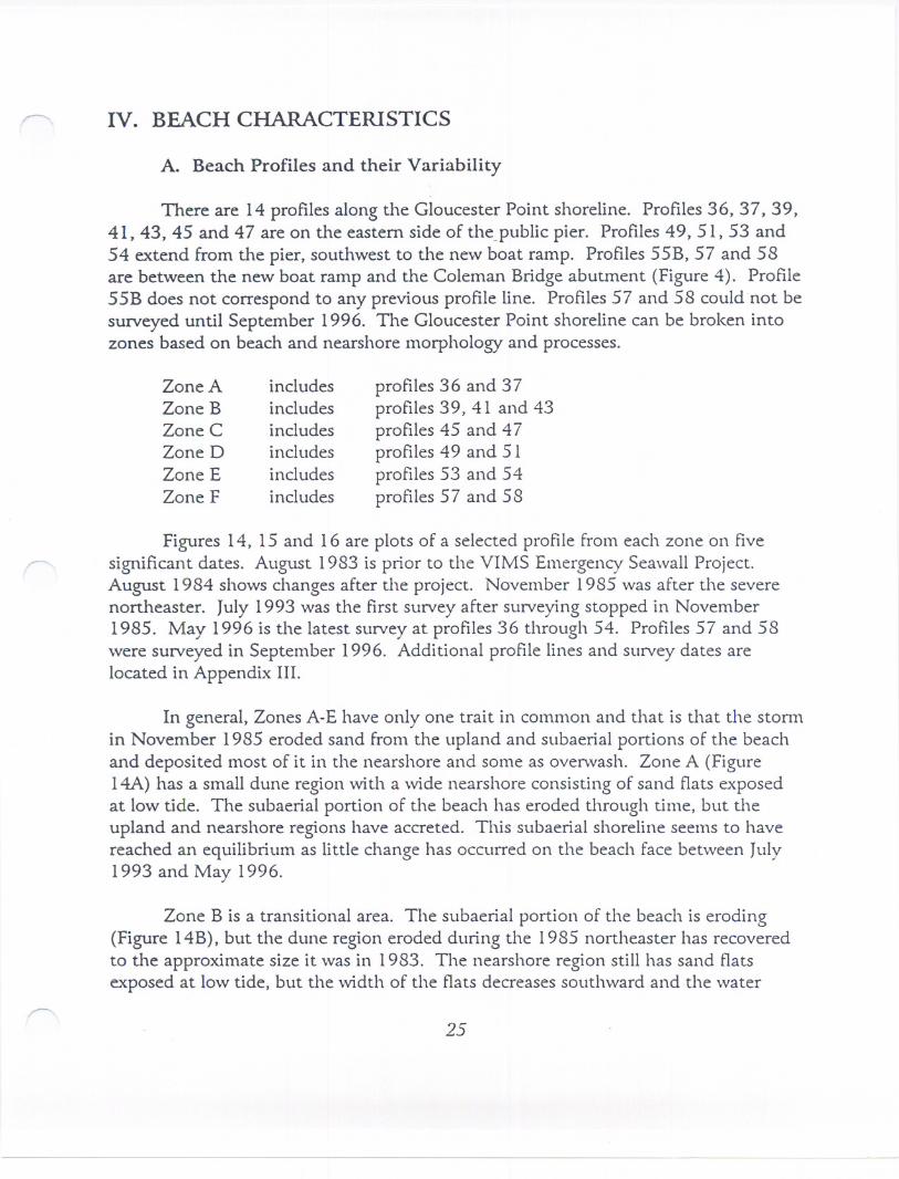
There are 14 profiles along the Gloucester Point shoreline. Profiles 36, 37, 39,41,43,45 and 47 are on the eastern side of the_public pier. Profiles 49, 51, 53 and54 extend from the pier, southwest to the new boat ramp. Profiles 55B, 57 and 58are between the new boat ramp and the Coleman Bridge abutment (Figure 4). Profile55B does not correspond to any previous profile line. Profiles 57 and 58 could not besurveyed until September 1996. The Gloucester Point shoreline can be broken intozones based on beach and nearshore morphology and processes.

Zone AZone BZone CZone DZone EZone F

includesincl udesincludesincludesincludesincludes

profiles 36 and 37profiles 39, 41 and 43profiles 45 and 47profiles 49 and 51profiles 53 and 54profiles 57 and 58

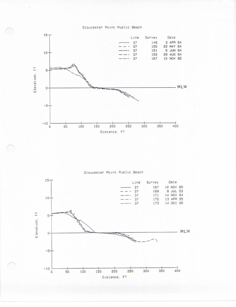
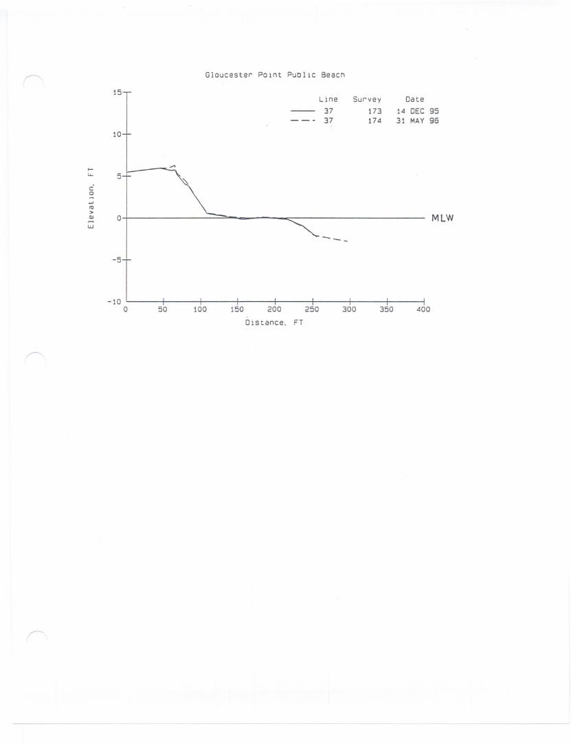
Figures 14, 15 and 16 are plots of a selected profile from each zone on fivesignificant dates. August 1983 is prior to the VIMS Emergency Seawall Project.August 1984 shows changes after the project. November 1985 was after the severenortheaster. July 1993 was the first survey after surveying stopped in November1985. May 1996 is the latest survey at profiles 36 through 54. Profiles 57 and 58were surveyed in September 1996. Additional profile lines and survey dates arelocated in Appendix III.

In general, Zones A-E have only one trait in common and that is that the stonnin November 1985 eroded sand from the upland and subaerial portions of the beachand deposited most of it in the nearshore and some as overwash. Zone A (Figure14A) has a small dune region with a wide nearshore consisting of sand flats exposedat low tide. The subaerial portion of the beach has eroded through time, but theupland and nearshore regions have accreted. This subaerial shoreline seems to havereached an equilibrium as little change has occurred on the beach face between July1993 and May 1996.

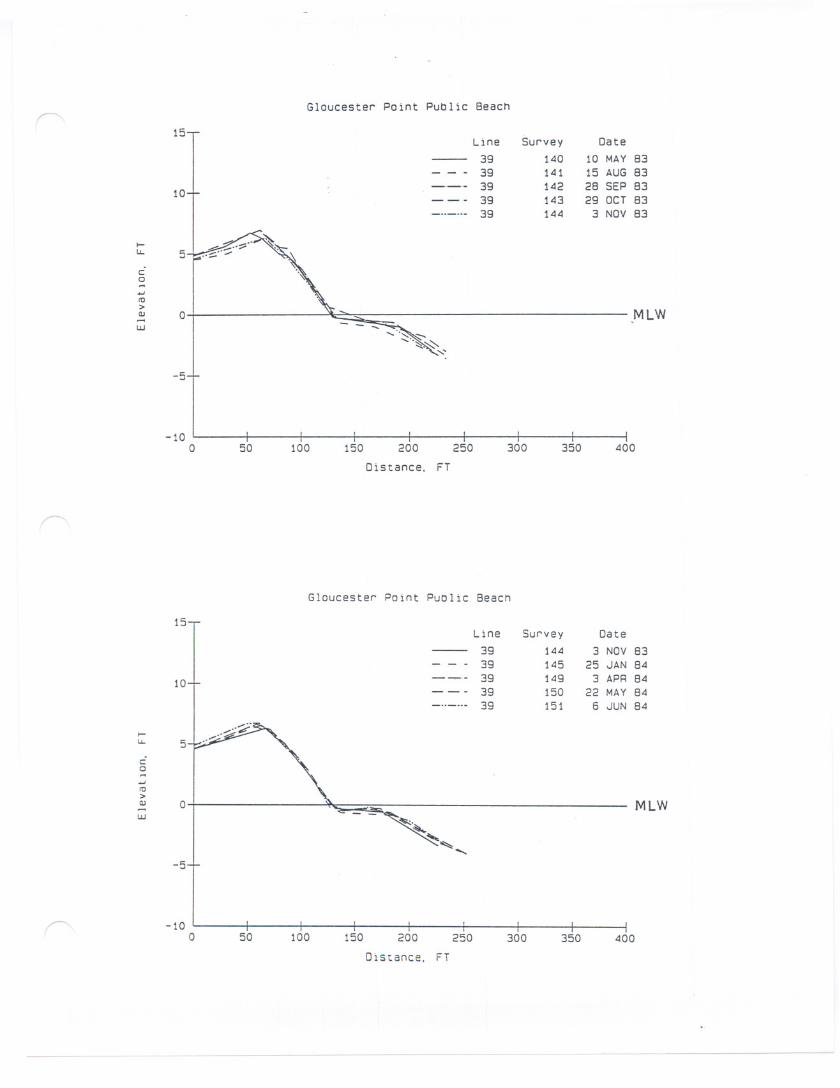
Zone B is a transitional area. The subaerial portion of the beach is eroding(Figure 14B), but the dune region eroded during the 1985 northeaster has recoveredto the approximate size it was in 1983. The nearshore region still has sand flatsexposed at low tide, but the width of the flats decreases southward and the water

25

-10o 50 100 150 200 250

Distance. FT

300 350 400

-5

-10o 50 100 150 200 250 300 350 400

Distance. FT

Figure 14. Plot depicting change at A.) profile 37 in Zone A and B.) profile 41 inZone B.

26

Gloucester Point Public 8eacn

15 ,Line Survey Date

37 141 15 AUG 8337 152 28 AUG 84

10+37 167 10 NQV 8537 169 8 JUL 9337 174 31 MAY 96

..... .-----... ./

u- 5 ,-. 'c <, A0 '.-->J \ ".<0> '----.-.. MLW(II 0- '.W :-..,

:0.. ........-

I

.... ..-

-5

Gloucester Point Public 8each

15

10

Line

4747474747

Survey141152167169174

Date15 AUG 8328 AUG 8410 NDV 85B JUL 93

31 MAY 96

A

-5

-10o 50 100 150 200 250

Distance. FT

300 350 400

-5

-10a 50 100 150 200 250 300 350 400

Distance. FT

Figure 15. Plot depictingchange at A.) profile47 in Zone C and B.) profile51 inZone D.

27

l-lL. 5

C0.

II]>

01 " '. MLW111-W

-5

-10o .50 100 150 200 250 300 350 400

Distance. FT

-10o 150 200 250

Distance. FT

Figure 16. Plot depicting change at A.) profile 54 in Zone E and B.) profile 58 inZone F.

50 100 300 350 400

28

Gloucester Point Public 6each

15 .Line Survey Date

54 141 15 AUG 6354 152 26 AUG 64

10+54 167 10 NOV 6554 169 6 JUL 9354 174 31 MAY 96

, .... A.....

11.. 5

C0

.....

IV

MLW>0' \\ '\ '.OJ

....W

becomes deeper closer to shore. Zone C includes the public pier. The pier is aminimal littoral barrier, but it does partially stabilize the nearshore. This zone hasdeveloped a wide dune since 1983 (Figure 15A). The subaerial and nearshore regionshave experiencedlittle change except for the stonn profileafter tl1e 1985 nortl1easter.

Zone D is another transitional area. Profiles 49 and 51 differ in that profile 49has developed a wide dune area since 1983 (Appendix III). However, both profileshave experienced little other change in profile snape (Figure 15B) (excluding thestonn profile). This zone is near tl1e point and represents a change from a wide,shallow nearshore region to a narrower nearshore and steep drop-off to the York Riverchannel which is closer to shore at this southen1 part of the beach.

Zones E and F were affected most by the widening of the Coleman Bridge.The upper beach at profiles 53 and 54 was used as a holding place for constructionmaterials and equipment. Also the construction of the new boat ramp changed theconfiguration of the shoreline. Profiles 57 and 58 originally were tied to a woodenbulkhead which was removed during the bridge work. The new boat ramp changedthe littoral processes of the point. Prior to its installation, sand would be transportedsouthward along the public beach, around the point where it would accumulateagainst the bridge abutment or fall into the York River channel (Skrabal, 1987). Thenew boat ramp effectively stopped the transport around the point. Profiles 53 and54, Zone E, were eroding between 1983 to 1993 (Appendix III and Figure 16A).However, after the boat ramp was constructed, sand accumulated against it. Sandcannot move around the boat ramp since the end of the boat ramp bulld1ead is indeep water near the York River channel. Profiles 57 and 58, Zone F (Figure 16B),accreted between 1983 and 1993. However, between 1993 and 1996, these profileshave lost sand probably due to constnlction and the elimination of the updrift sandsupply.

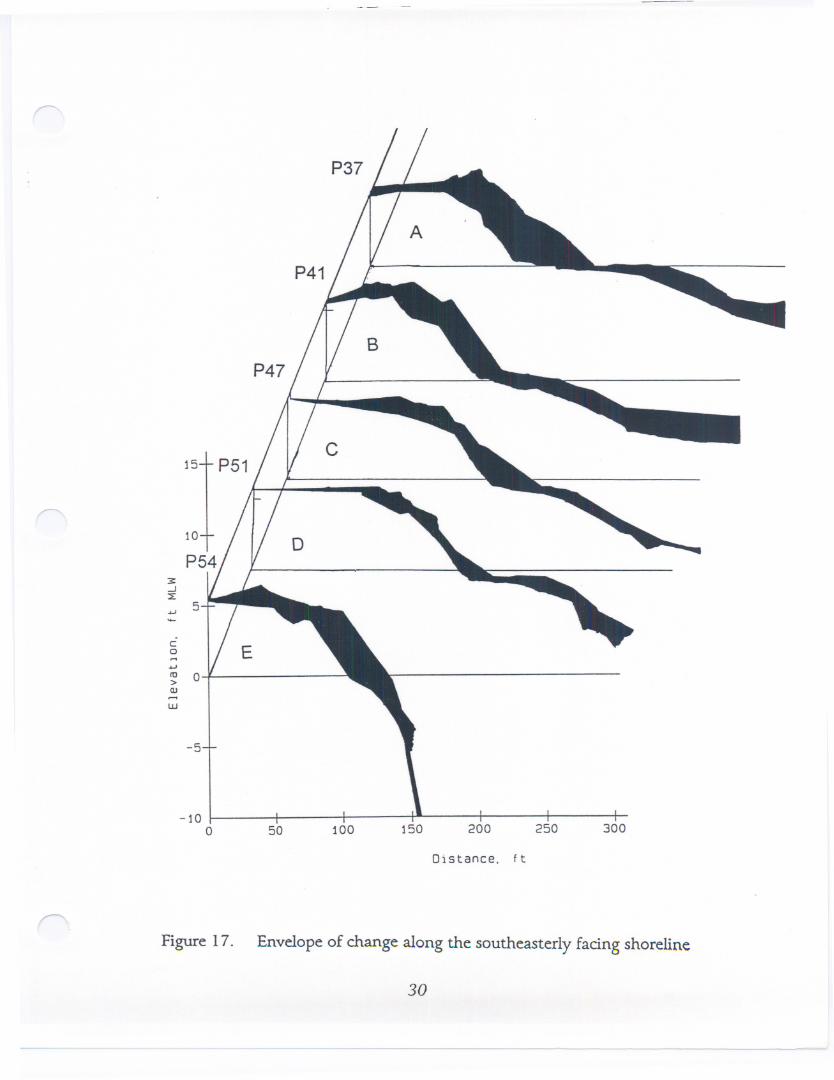
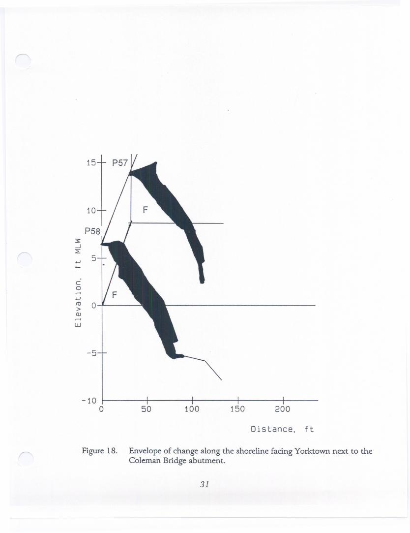
The overall variation in the profiles is shown in Figures 17 and 18. Thesefigures show the envelope of change from the baseline into the nearshore regionbetween 1983 and 1996. Figure 17 shows a profile from Zones A-E. In Zone A, aconsiderable amount of total beach change occurred in the backshore, foreshore andnearshore regions. Zone B has characteristics of both Zone A and C and is labeled atransition zone. Zone C had little change in the nearshore and some change in theupland area. The foreshore changes are mostly the result of the November 1985stonn. Zone D had little change, and the nearshore region is getting deeper. Zone Ehas had substantial change along the profile, and the nearshore region drops offquickly into the York River channel. Figure 18 shows profiles 57and 58 from ZoneF and describes the envelope of change at the point as well as the steep drop-off in

29

- - - - - - - - -

15c

-10o 50 100 150 200 250 300

Distance. f t

,-

Figure 17. Envelope of change along the southeasterly facing shoreline

30

- ---- - - - - - - - - - - - --

10 I I I I

3: P5,4/ Y

0

...J::E

..., 5

.....

C0 1/... E...,It) 0>w......w

-5

-10 _

o 50 100 150 200

Distance. ft

Figure lB. Envelope of change along the shoreline facing Yorktown next to theColeman Bridge abutment.

31

--.J

.j...J5

....

c0.r-1.j...J

co 0>QJ......

W

the nearshore region.

B. Variability in Shoreline Position

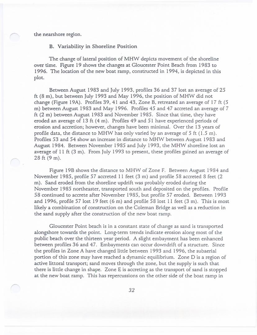
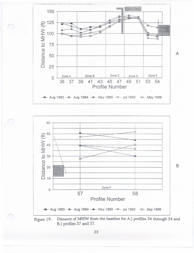
The change of lateral position of MHW depicts movement of the shorelineover time. Figure 19 showsthe changesat GloucesterPoint Beachfrom 1983 to1996. The location of the new boat ramp, constructed in 1994, is depicted in thisplot.

Between August 1983 and July 1993, profiles 36 and 37 lost an average of 25ft (8 m), but between July 1993 and May 1996, the position of MHW did notchange (Figure 19A). Profiles 39, 41 and 43, Zone B, retreated an average of 17 ft (5m) between August 1983 and May 1996. Profiles 45 and 47 accreted an average of 7ft (2 m) between August 1983 and November 1985. Since that time, they haveeroded an average of 13 ft (4 m). Profiles 49 and 51 have experienced periods oferosion and accretion; however, changes have been minimal. Over the 13 years ofprofile data, the distance to MHW has only varied by an average of 5 ft (1.5 m).Profiles 53 and 54 show an increase in distance to MHW between August 1983 andAugust 1984. Between November 1985 and July 1993, the MHW shoreline lost anaverage of II ft (3 m). From July 1993 to present, these profiles gained an average of28 ft (9 m).

Figure 19B shows the distance to MHW of Zone F. Between August 1984 andNovember 1985, profile 57 accreted II feet (3 m) and profile 58 accreted 8 feet (2m). Sand eroded from the shoreline updrift was probably eroded during theNovember 1985 northeaster, transported south and deposited on the profiles. Profile58 continued to accrete after November 1985, but profile 57 eroded. Between 1993and 1996, profile 57 lost 19 feet (6 m) and profile 58 lost II feet (3 m). This is mostlikely a combination of constnlction on the Coleman Bridge as well as a reduction inthe sand supply after the construction of the new boat ramp.

Gloucester Point beach is in a constant state of change as sand is transportedalongshore towards the point. Long-tenn trends indicate erosion along most of thepublic beach over the thirteen year period. A slight embayment has been enhancedbetween profiles 36 and 47. Embayments can occur downdrift of a stnlcture. Sincethe profiles in Zone A have changed little between 1993 and 1996, the subaerialportion of this zone may have reached a dynamic equilibrium. Zone D is a region ofactive littoral transport; sand moves through the zone, but the supply is such thatthere is little change in shape. Zone E is accreting as the transport of sand is stoppedat the new boat ramp. This has repercussions on the other side of the boat ramp in

32

- Aug 1983 ~ Aug 1984 -0-- Nov 1985 ~ Jul1993 -s- May 1996

60

---50.::::=-...-

S 40I~o 30

~

(1)C,,)c 20ro

~(/).-o 10

i:!:

B

o Zone F

57 58Profile Number

--- Aug 1983 ~ Aug 1984 -- Nov 1985 --Q- Jul 1993 -e-- Sap 1996

Figure 19. Distance of MHW from the baseline for A.) profiles 36 through 54 andB.) profiles 57 and 57.

33

- - -

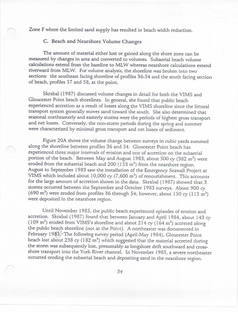
--Zone F where the limited sand supply has resulted in beach width reduction.

C. Beach and Nearshore Volume Changes

The amount of material either lost or gained along the shore zone can bemeasured by changes in area and converted to volumes. Subaerial beach volumecalculations extend from the baseline to MLW whereas nearshore calculations extendriverward from MLW. For volume analysis, the shoreline was broken into twosections: the southeast facing shoreline of profiles 36-54 and the south facing sectionof beach, profiles 57 and 58, at the point.

Skrabal (1987) discussed volume changes in detail for both the VIMS andGloucester Point beach shorelines. In general, she found that public beachexperienced accretion as a result of losses along the VIMS shoreline since the littoraltransport system generally moves sand toward the south. She also determined that

seasonal northeasterly and easterly storms were the periods of highest gross transportand net losses. Conversely, the non-storm periods during the spring and summerwere characterized by minimal gross transport and net losses of sediment.

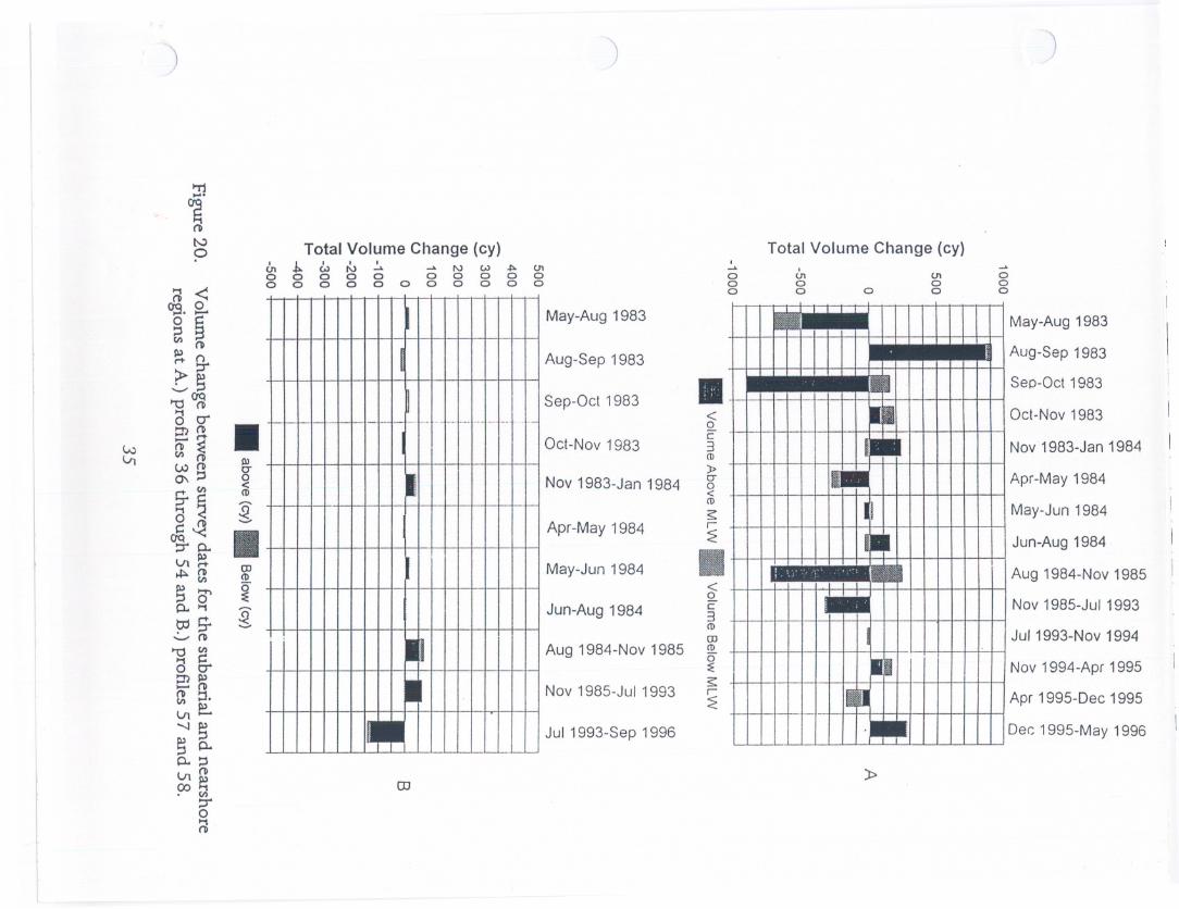
Figure 20A shows the volume change between surveys in cubic yards summedalong the shoreline between profiles 36 and 54. Gloucester Point beach hasexperienced three major intervals of erosion and one of accretion on the subaerialportion of the beach. Between May and August 1983, about 500 cy (382 m3) wereeroded from the subaerial beach and 200 (153 m3) from the nearshore region.August to September 1983 saw the installation of the Emergency Seawall Project atV1MS which included about 10,000 cy (7,600 m3) of renourishment. This accountsfor the large amount of accretion shown in the data. Skrabal (1987) showed that 3

storms occurred between the September and October 1983 surveys. About 900 cy(690 m3) were eroded from profiles 36 through 54; however, about 150 cy (l15 m3)were deposited in the nearshore region.

Until November 1985, the public beach experienced episodes of erosion and

accretion. Skrabal (1987) found that between January and April 1984, about 143 cy(109 m3) eroded from VIMS's shoreline and about 214 cy (l64 m3) accreted alongthe public beach shoreline (not at the Point). A northeaster was documented in

February 19@oThe following survey period (April-May 1984), Gloucester Pointbeach lost about 238 cy (182 m3) which suggested that the material accreted duringthe storm was subsequently lost, presumably as longshore drift southward and cross-shore transport into tl1e York River channel. In November 1985, a severe northeaster

occurred eroding the subaerial beach and depositing sand in the nearshore region.

34

-----

Total Volume Change (cy)~ ~ W N ~ ~ N W A ~o 0 000 0 0 000o 0 0 0 0 000 000

OJ

Total Volume Change (cy).

~ooo

I~

oo o

~oo

»

~

ooo

May-Aug 1983

Aug-Sep 1983

Sep-Oct 1983

Oct-Nov 1983

Nov 1983-Jan 1984

Apr -May 1984

May-Jun 1984

Jun-Aug 1984

Aug 1984-Nov 1985

Nov 1985-Jul 1993

Jul 1993-Nov 1994

Nov 1994-Apr 1995

Apr 1995-Dec 1995

Dee 1995-May 1996

ITj

l'9

ii -<0,9 0

a' §su I')

fg'"OC1Q'"1 I')o cr::nl') IIw a-v, WI') Q)

0\::3C"a

go en

<(I)

8,...,

g- 11Vt,.....t:>- en

(I)

crp..'"1go ;g:

......... I')

'"0 en8 g.::nsua- B,Vt-..J

p..p..::3Vtl')c:o, en

5ii

I

I

-. I- - -- - _. ._- - -- ...- .- -.. -- -

I

I

. , --

I.

May-Aug1983

Aug-Sep 1983

Sep-Oct 1983 II<a

Oct-Nov 1983c3(I)

»Nov 1983-Jan 1984

C"a<(I)

Apr -May 1984r

lEiMay-Jun 1984

<aJun-Aug 1984

c3(I)en

Aug 1984-Nov 1985 (I)0":E

Nov 1985-Jul 1993 r

Jul 1993-Sep 1996

-- _I--I.II

--*..--

-I- - --..,

The volume data between November 1985 and July 1993 are probably themost indicative of long-term shoreline trends. A net of just over 300 cy (230 m3) waseroded over a seven to eight year period. Very little net change occurred in thenearshore region between these dates. Between July 1993 and December 1995,volume changewasvariable;however,between December 1995 and May 1996, thesubaerial beach accreted. This is due to the end of construction on the Coleman

Bridge and stacking up of sand along profiles 53 and 54.

Figure 20B shows the volume changes at the Point utilizing data from profiles57 and 58. Volumetric changes were variable between May 1983 and August 1984.Between August 1984 and November 1985, profiles 57 and 58 gained about 55 cy(42 m3) on their subaerial beach 15 cy (11 m3) in the nearshore indicating transportto the south around the Point, especially during storms. Between 1985 and 1993,these subaerial beach on these profiles accreted creating a high berm while thenearshore underwent very slight erosion. This is probably indicative of long-termtrends along this shoreline. However, between 1993 and 1996, severe erosion alongthese profiles occurred due to bridge construction and the constmction of the newboat ramp which limited the sand supply to the Point.

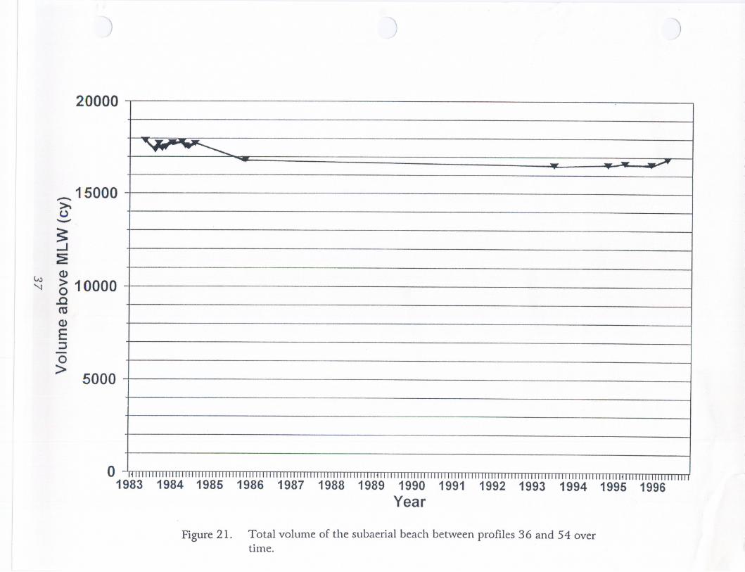
Figure 21 describes the total volume change between profile 36 and 54 throughtime. In general, the long-term trend is slight erosion along the Gloucester Pointpublic beach shoreline until the last survey. The last survey shows a slight increase involume. This is probably due to sand accumulating against the boat ramp; however,once the limit to how much material can be stored against the boat ramp is reached,most of the sand transported into Zone E will be transported offshore and lost to thesystem.

36

)

20000

~~ - - -~

_ 15000~o-

W'J

~...J

~Q)

~ 10000.croQ)E:J-o>

5000

o 11111111111111111111111111111111111111111111111111T11111111111111111111111i 111111111111111111111111111111111111111111111111111111111111111lHn 111111111111111111111111

1983 1984 1985 1986 1987 1988 1989 1990 1991 1992 1993 1994 1995 1996Year

Figure21. Total volume of the subaerial beach between profiles 36 and 54 overtime.

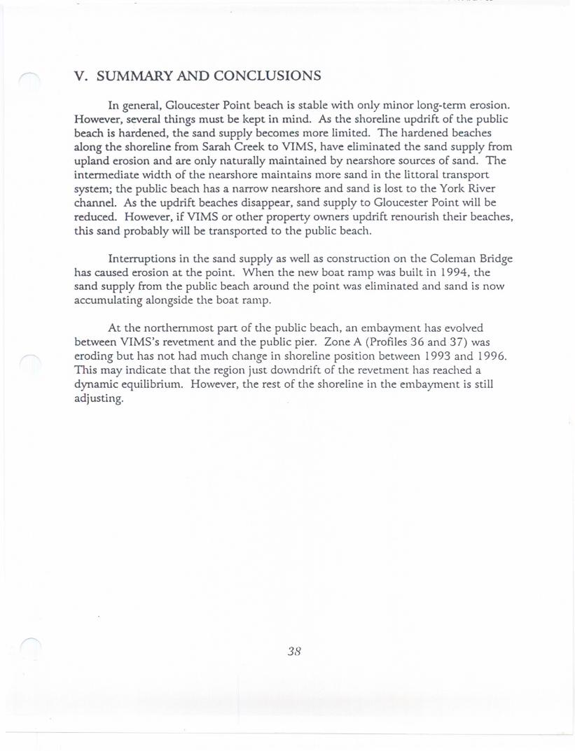
v. SUMMARY AND CONCLUSIONS

In general, Gloucester Point beach is stable with only minor long-term erosion.However, several things must be kept in mind. As the shoreline updrift of the publicbeach is hardened, the sand supply becomes more limited. The hardened beachesalong the shoreline from Sarah Creek to VIMS, have eliminated the sand supply fromupland erosion and are only naturally maintained by nearshore sources of sand. Theintermediate width of the nearshore maintains more sand in the littoral transportsystem; the public beach has a narrow nearshore and sand is lost to the York Riverchannel. As the updrift beaches disappear, sand supply to Gloucester Point will bereduced. However, if VIMS or other property owners updrift renourish their beaches,this sand probably will be transported to the public beach.

Interruptions in the sand supply as well as construction on the Coleman Bridgehas caused erosion at the point. When the new boat ramp was built in 1994, thesand supply from the public beach around the point was eliminated and sand is nowaccumulating alongside the boat ramp.

At the northernmost part of the public beach, an embayment has evolvedbetween VIMS's revetment and the public pier. Zone A (Profiles 36 and 37) waseroding but has not had much change in shoreline position between 1993 and 1996.This may indicate that the region just downdrift of the revetment has reached adynamic equilibrium. However, the rest of the shoreline in the embayment is stilladjusting.

38

VI. RECOMMENDATIONS

Presently, a bulkhead is being constructed between tl1e new boat ramp and tl1eColeman Bridge Abutment. This project is intended to protect tl1e parking lot andthe road to the boat ramp from further erosion. The public pier was destroyed andthe new boat ramp was damaged during the passage of Hurricane Fran in September1996. These facilities should be repaired as they are a hazard and will continue todeteriorate unless cared for.

In order to stabilize the shore at the border between VIMS and the Gloucester

Point beach, we recommend a low, rock spur. This would allow the entire shorebetween the VIMS revetment and the public pier to evolve into a state of dynamicequilibrium. With the source of sand to the public beach reduced, Gloucester Countyshould consider maintaining the existing beach planfonn. A low, reef breakwater atthe pier and a spur at the boat ramp would stabilize the beach planfonn over thelong-tenn.

39

- - - - - --

VII. REFERENCES

Anderson, G.L., G.B. Williams, M.H. Peoples, and L. Weishar, 1976. ShorelineSituation Report, GloucesterCounry, Virginia. ~RAMSOE No. 83. VirginiaInstitute of Marine Science, College of William and Mary, Gloucester Point,Virginia, 71 pp.

Bascom, W.N., 1959. The relationship between sand size and beach face slope. Am.Geophys.Union Transactions32(6):866-874.

Boon, J.D., C.S. Welch, H.S. Chen, RJ. Lukens, C.S. Fang, and J.M. Zeigler, 1978.A Stann SurgeModel Stut[y, Vol. 1. Stonn SurgeHeight-FrequenryAnalysis andModel Predictionfor ChesapeakeBqy. SRAMSOE No. 189. Virginia Institute ofMarine Science, College of William and Mary, Gloucester Point, Virginia, 149pp + app.

Bretschneider, C.L., 1952. The generation and decay of wind waves in deep water.Transactionsof theAmeric.anGeopl!ysic:alUnion, 33: 381-389.

Bretschneider, C.L., 1958. Revisions in wave forecasting: Deep and shallow water.Proceedings Sixth Conf. on Coastal Engineering, ASCE, Council on WaveResearch.

Byrne, RJ. and G.L. Anderson, 1977. ShorelineErosionin TidewaterVirginia. SpecialReport in Applied Marine Science and Ocean Engineering, No. Ill. VirginiaInstitute of Marine Science, Gloucester Point, VA, 102 pp.

Ebersole, B.A., M.A. Cialone, and M.D. Prater, 1986. RCPWA VE - A Linear WavePropagationModelfor EngineeringUse. CERC-86-4, U.S. Anny Corps ofEngineers Report, 260 pp.

Folk, RL., 1980. Petrology of Sedimentary Rocks. Hemphill Publishing Co., AustinTX, 182 pp.

Friedman, G.M. and J.E. Sanders, 1978. Principles of Sedimentology. John Wileyand Sons, New York, 792 pp.

40

Hardaway, C.S., Jr., G.R. Thomas, and J.H. D, 1991. ChesapeakeBqy ShorelineStudies:HeadlandBreakwatersand PocleetBeachesfor ShorelineErosionControl. SRAMSOENo. 313, Virginia Institute of Marine Science, College of William and Mary,Gloucester Point, VA, 153 pp.

Hardaway, C.S., Jr., D.A. Milligan and G.R. Thomas, 1993. PublicBeachAssessmentReport: Cape CharlesBead" Town of Cape Charles,Virginia. Technical Report,Virginia Institute of Marine Science, College of William and Mary, GloucesterPoint, VA, 42 pp. + app.

Kiley, K., 1982. Estimates of bottom water velocities associated with gale windgenerated waves in the James River, Virginia. Virginia Institute of MarineScience, School of Marine Science, College of William and Mary, GloucesterPoint, VA.

Komar, P.D., 1976. Beach Processesand Sedimentation. Prentice-Hall, Inc., EnglewoodCliffs, NJ, 429 pp.

Milligan, D.A., C.S. Hardaway, Jr., and G.R. Thomas, 1995. PublicBeachAssessmentReport:Huntington Park Beach,AndersonPark Beach,and King-LincolnPark Beach,Ci9' of Newport News, Virginia. Technical Report, Virginia Institute of MarineScience, College of William and Mary, Gloucester Point, VA, 60 pp. + app.

Skrabal, T.E., 1987. ~ystemResponseof a NourishedBeachin a Low-Energyl:.stuarineEnvironment, GloucesterPoint, Virginia. Unpublished Masters thesis, VirginiaInstitute of Marine Science, College of William and Mary, Gloucester Point,Virginia, 117 pp.

Stauble, D.K., A.W. Garcia, N.C. Kraus, W.G. Grosskopf, and G.P. Bass, 1993. BeachNourishment Project ReJponse and Design Evaluation: Ocean City, Maryland.Technical Report CERC-93-13, Coastal Engineering Research Center, U.S. Army Corpsof Engineers WatelWaysExperiment Station, Vicksburg, MS.

Suh, K.D, 1990. WINDOW Program. Virginia Institute of Marine Science, Collegeof William and Mary, Gloucester Point, Virginia.

Sverdrup, H.U. and W.H. Munk, 1947. Wind sea, and swell: Theory of relations forforecasting. U.S. Navy Hydrographic Office Publ. No. 60 I.

Tidelog, 1996. Chesapeake Tidewater. Pacific Publishers, Bolinas, CA.

41

U.S. Anny Corps of Engineers, 1977. ShoreProtectionManual. Coastal EngineeringResearch Center, Fort Belvoir, Virginia.

U.S. Anny Corps of Engineers, 1984. ShoreProtectionManual. U.S. GovernmentPrinting Office, Washington, D.C.

U.S. Anny Corps of Engineers, 1993. Shoreline Erosion Stz.u!y,Fort Eustis, Virginia.Norfolk District.

Wright, 1.0., C.S. Kim, C.S. Hardaway, Jr., S.M. Kimball, and M.O. Green, 1987.Shorefaceand Beach D.ynamic:sof the Coastal Regionfrom Cape Henry to False Cape,Virginia. Technical Report, Virginia Institute of Marine Science, College ofWilliam and Mary, Gloucester Point, Virginia, 116 pp.

42

APPENDIX I

Gloucester Point Public Beach Sediment Data

Gloucester Point Sample Analvsis:gean

RSA results-Sand portionDate Number Location 0/0gravel %sancJ Yosllt Yoclay %mucJ MecJian sortino Skewness KurtosIS

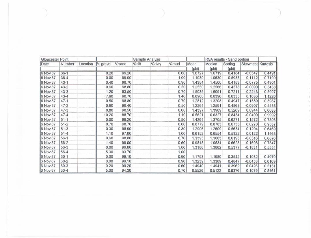
(phi) (phi)(PhtM6 Nov 87 36-1 0.20 99.20 0.60 1.6727 1.6719 0.4 -0.0547 0.4491

6 Nov 87 36-4 0.00 99.00 1.00 1.1030 1.0630 0.5935 0.1112 0.71006 Nov 87 43-1 0.40 98.70 0.90 1.4384 1.4500 0.4183 -0.0775 0.49016 Nov 87 43-2 0.60 98.80 0.50 1.2550 1.2566 0.4578 -0.0090 0.54386 Nov 87 43-3 1.20 93.50 0.70 1.5035 1.6091 0.7211 -0.2243 0.59276 Nov 87 43-4 7.90 90.70 1.40 0.8960 0.8396 0.6335 0.1636 1.12206 Nov 87 47-1 0.50 98.80 0.70 1.2812 1.3208 0.4947 -0.1559 0.59876 Nov 87 47-2 0.90 99.40 0.50 1.2264 1.2591 0.4868 -0.0907 0.5458--- ---- ---.-.--- ------- --_.6 Noy87__ 47-3 0.80 98.50 0.60 1.4397 1.3909 0.5269 0.0944 0.6033--- ---6 Nov 87 47-4 10.20 88.70 1.10 0.5621 0.6327 0.8434 -0.0400 0.99926 Nov 87 51-1 0.00 99.20 0.80 1.4264 1.3705 0.6271 0.1572 0.78086 Nov 87 51-2 0.70 98.70 0.60 0.8779 0.8783 0.6733 0.0270 0.95376 Nov 87 51-3 0.30 98.90 0.80 1.2906 1.2609 0.5634 0.1204 0.64696 Nov 87 51-4 1.10 97.80 1.00 0.6152 0.6554 0.5322 0.0122 1.14686 Nov87 56-1 0.60 98.80 0.70 1.1395 1.1663 0.6193 -0.0516 0.68766 Nov 87 56-2 1.40 98.00 0.60 0.9848 1.0534 0.6628 -0.1695 0.75476 Nov 87 56-3 0.00 99.00 1.00 1.3186 1.3862 0.5377 -0.1831 0.55546 Nov 87 56-4 5.30 93.70 1.006 Nov 87 60-1 0.00 99.10 0.90 1.1793 1.1980 0.3542 -0.1032 0.49706 Nov 87 60-2 0.00 99.10 0.90 1.3239 1.3309 0.4847 -0.0458 0.61696 Nov 87 60-3 0.20 99.20 0.60 1.4940 1.4941 0.3962 0.0426 0.51316 Nov 87 60-4 5.00 94.30 0.70 0.5526 0.5122 0.6376 0.1079 0.8461

Gloucester Point Sample AnalvsisRSA results -Sandpo:;nIDate INumber Location VoQravel %sand "Iosilt I"IoClav %mud Mean Median sorting ewness KurtosIS

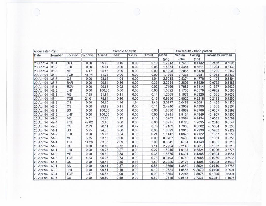
(phi) (phi) (phi)20 Apr 94 36-1 BOD 0.00 99.90 0.10 0.00 0.10 1.7213 1.7410 0.4132 -0.2486 0.509620 Apr 94 36-2 LHT 0.00 99.94 0.06 0.00 0.06 1.5354 1.5384 0.5611 0.1924 0.813920 Apr 94 36-3 MB 4.17 95.83 0.00 0.00 0.00 0.1995 0.2065 0.3428 -0.1209 1.014220 Apr 94 36-4 TOE 48.74 51.26 0.00 0.00 0.00 1.1665 0.7331 1.2981 0.4078 0.633020 Apr 94 36-5 OS 0.00 98.96 1.04 0.00 1.04 2.5035 2.5374 0.4776 -0.1121 0.339420 Apr 94 36-6 BAR 0.00 99.64 0.36 0.00 0.36 2.2684 2.2807 0.3529 -0.0762 0.318520 Apr 94 43-1 EOV 0.00 99.98 0.02 0.00 0.02 1.7166 1.7687 0.5114 -0.1367 0.5639

gQ.AQfh4 43-2 LHT 0.00 100.00 _.QJHL__...QQQ- 0.00 -1 ---1:§.735 0.6579 -0.0902 0.5885.__. .__8 -- - -.-- .- ._---_._- _._--20 AQf94_ 43-3 MB 7.95 91.94 0.11 0.00 0.11 1.2069 1.1071 0.8320 0.1685 0.7638.----- __0.- -----20 AQr94 . 43-4 TOE 21.01 78.84 0.16 0.00 0.16 0.9986 0.9022 0.9218 0.2113 0.7260--- --20 Apr 94 43-5 OS 0.00 96.60 1.46 1.94 - 3.40 2.0377 2.0457 0.5051 -0.1425 0.433020 Apr 94 43-6 OS 0.00 99.89 0.11 0.00 0.11 2.4240 2.3939 0.4396 0.1353 0.330420 Apr 94 47-1 BS 0.00 100.00 0.00 0.00 0.00 1.8030 1.8087 0.3789 -0.0357 0.399720 Apr 94 47-2 LHT 0.00 100.00 0.00 0.00 0.00 1.8745 1.9164 0.4349 -0.1967 0.440020 ADr94 47-3 MD 9.61 89.26 1.13 0.00 1.13 1.3463 1.3994 0.9434 0.0589 0.859920 Apr 94 47-4 TOE 47.02 52.98 0.00 0.00 0.00 1.3975 1.6728 1.2895 -0.2310 0.6544.20 ADr94 47-5 OS 2.93 96.31 0.28 0.47 0.76 1.7162 1.7688 0.3062 -0.3384 0.333020 Apr 94 51-1 BS 5.25 94.75 0.00 0.00 0.00 1.0029 1.3015 0.7930 -0.3953 0.712920 Apr 94 51-2 LHT 0.00 99.76 0.24 0.00 0.24 1.1142 1.0876 0.7122 0.1357 0.895920 Apr 94 51-3 MB 6.85 93.15 0.00 0.00 0.00 0.9767 0.9493 0.8669 0.1061 0.835520 Apr 94 51-4 TOE 14.28 83.63 2.09 0.00 2.09 0.6841 0.6761 0.4149 0.0305 0.931820 ADr94 51-5 OS 0.00 98.86 0.72 0.42 1.14 2.2294 2.2140 0.3617 0.1033 0.331020 Apr 94 54-1 LHT 0.00 99.73 0.27 0.00 0.27 1.8945 1.9137 0.3524 -0.0996 0.377520 Apr 94 54-2 MB 0.00 99.62 0.38 0.00 0.38 1.6375 1.6391 0.4388 -0.0394 0.495120 Apr 94 54-3 TOE 4.23 95.05 0.73 0.00 0.73 0.9493 0.9780 0.7088 -0.0259 0.693520 Apr 94 54-4 OS 0.00 98.48 0.85 0.66 1.52 2.2226 2.2176 0.4305 -0.0023 0.406920 Apr 94 60-1 BS 0.00 99.44 0.37 0.19 0.56 1.3669 1.3850 0.5624 0.0749 0.775820 ADr94 60-2 LHT 0.00 99.81' 0.19 0.00 0.19 1.9524 1.9568 -0.2679 -0.0496 0.299120 Apr 94 60-4 TOE 3.47 96.53 0.00 0.00 0.00 1.3364 1.2948 0.5975 0.1205 0.639420 Apr 94 60-5 OS 0.00 99.50 0.50 0.00 0.50 1.0515 0.9848 0.7327 0.3251 1.1093

Gloucester Point Sample Analvsis RSA results-Sand portionDate Number Location Yogravel I%sana %Sllt %Clay %mua Mean Mealan Isortino SKewnessIKurtosIS

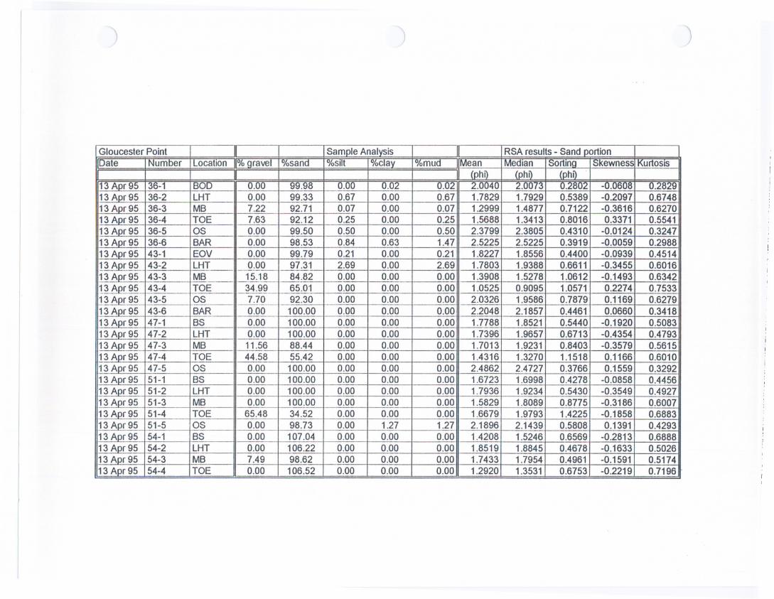
(phi) (phi) (phi)13 Apr 95 36-1 BOD 0.00 99.98 0.00 0.02 0.02 2.0040 2.0073 u.ou -0.060813 Apr 95 36-2 LHT 0.00 99.33 0.67 0.00 0.67 1.7829 1.7929 0.5389 -0.2097 0.674813 Apr 95 36-3 MB 7.22 92.71 0.07 0.00 0.07 1.2999 1.4877 0.7122 -0.3616 0.627013 Apr 95 36-4 TOE 7.63 92.12 0.25 0.00 0.25 1.5688 1.3413 0.8016 0.3371 0.554113 Apr 95 36-5 OS 0.00 99.50 0.50 0.00 0:50 2.3799 2.3805 0.4310 -0.0124 0.324713 Apr 95 36-6 BAR 0.00 98.53 0.84 0.63 1.47 2.5225 2.5225 0.3919 -0.0059 0.298813 Apr 95 43-1 EOV 0.00 99.79 0.21 0.00 0.21 1.8227 1.8556 0.4400 -0.0939 0.451413 Apr 95 43-2 LHT 0.00 97.31 2.69 0.00 2.69 1.7803 1.9388 0.6611 -0.3455 0.6016--13 Apr 95 43-3 MB -15.JL. 84J!L 0.00 0.00 0.00 1.3908 1.5278 1.0612 -0.1493 0.634213 Apr 95 43-4 TOE 34.99 65.01 0.00 0.00 0.00 1.0525 0.9095 1.0571 0.2274 0.753313 Apr 95 43-5 OS 7.70 92.30 0.00 0.00 0.00 2.0326 1.9586 0.7879 0.1169 0.627913 Apr 95 43-6 BAR 0.00 100.00 0.00 0.00 0.00 2.2048 2.1857 0.4461 0.0660 0.341813 Aor 95 47-1 BS 0.00 100.00 0.00 0.00 0.00 1.7788 1.8521 0.5440 -0.1920 0.508313 Apr 95 47-2 LHT 0.00 100.00 0.00 0.00 0.00 1.7396 1.9657 0.6713 -0.4354 0.479313 Apr 95 47-3 MB 11.56 88.44 0.00 0.00 0.00 1.7013 1.9231 0.8403 -0.3579 0.561513 Aor 95 47-4 TOE 44.58 55.42 0.00 0.00 0.00 1.4316 1.3270 1.1518 0.1166 0.601013 Apr 95 47-5 OS 0.00 100.00 0.00 0.00 0.00 2.4862 2.4727 0.3766 0.1559 0.329213 Aor 95 51-1 BS 0.00 100.00 0.00 0.00 0.00 1.6723 1.6998 0.4278 -0.0858 0.445613 Apr 95 51-2 LHT 0.00 100.00 0.00 0.00 0.00 1.7936 1.9234 0.5430 -0.3549 0.492713 Aor 95 51-3 MB 0.00 100.00 0.00 0.00 0.00 1.5829 1.8089 0.8775 -0.3186 0.600713 Apr 95 51-4 TOE 65.48 34.52 0.00 0.00 0.00 1.6679 1.9793 1.4225 -0.1858 0.688313 Apr 95 51-5 OS 0.00 98.73 0.00 1.27 1.27 2.1896 2.1439 0.5808 0.1391 0.429313 Apr 95 54-1 BS 0.00 107.04 0.00 0.00 0.00 1.4208 1.5246 0.6569 -0.2813 0.688813Apr 95 54-2 LHT 0.00 106.22 0.00 0.00 0.00 1.8519 1.8845 0.4678 -0.1633 0.502613 Aor 95 54-3 MB 7.49 98.62 0.00 0.00 0.00 1.7433 1.7954 0.4961 -0.1591 0.517413 Apr 95 54-4 TOE 0.00 106.52 0.00 0.00 0.00 1.2920 1.3531 0.6753 -0.2219 0.7196 .

Gloucester Point Sample Analvsis RSA results-Sand portionIDate Number ILocation % gravel l%sana "IoSiit I"Ioelay %mua IMean MeaIan sortino skewnessIKurtosIS

(phi) (phi) (phi)114Dee 95 36-1 IBS 0.00 97.88 2.12 0.00 2.12 1.7173 1.6753 0.4127 0.1433 0.435114 Dee 95 36-2 LHT 0.00 98.36 1.64 0.00 1.6414 Dee 95 36-3 MB 1.82 96.78 1.40 0.00 1.40 1.3878 1.4102 0.6600 -0.0538 0.805814 Dee 95 36-4 TOE 27.28 70.85 1.87 0.00 1.87 0.8078 0.7641 0.8401 0.1458 0.796714 Dee 95 36-5 OS 0.00 99.56 0.44 0.00 0.44 2.4698 2.4554 0.5354 -0.0127 0.361914 Dee 95 43-1 BS 2.98 95.98 1.04 0.00 1.04 1.3814 1.5992 0.7907 -0.3502 0.656414 Dee 95 43-2 LHT 0.00 99.04 0.96 0.00 0.96 1.4090 1.3608 0.5465 0.1432 0.755714 Dee 95 43-3 MB 0.00 99.26 0.74 0.00 0.74 0.8932 0.8741 0.6022 0.2110 1.1024- -,,--_._. -----. --- -...._--_.- -_.- -.-...-. - ------ .-----14 Dee 95 43-4 TOE 53.89 45.11 1.00 0.00 1.00 0.5080 0.4669 0.6204 0.2443 1.275814 Dee 95 43-5 OS 0.00 97.86 2.14 0.00 2.14 1.7073 1.3367 1.6524 0.5878 0.473714 Dee 95 47-1 BS 2.19 97.48 -- 0.16 0.18 0.33 1.8640 1.8964 0.4835 -0.1317 0.499314 Dee 95 47-2 LHT Q- 99.8L 0.13 0.00 0.13 1.6663 1.6557 0.5716 -0.0435 0.6098-----_. -.---14 Dee 95 47-3 MB 15.24 84.57 -- 0.11 0.09 0.19 0.9823 0.8095 0.7786 0.3445 0.899414 Dee 95 47-4 TOE 46.08 53.19 0.72 0.00 0.72 2.0679 2.0644 0.7517 -0.0672 0.540514 Dee 95 51-1 BS 5.41 94.57 0.02 0.00 0.02 1.8344 1.8537 0.4989 -0.0655 0.468114 Dee 95 51-2 LHT 17.02 82.68 0.30 0.00 0.30 1.7547 1.7435 0.5985 -0.1176 0.643414 Dee 95 51-3 MB 12.90 86.67 0.04 0.39 0.43 0.5436 0.5534 0.5363 0.1092 1.123714 Dee 95 51-4 TOE 26.05 73.35 0.10 0.49 0.59 0.8744 0.5787 0.9779 0.5409 1.296314 Dee 95 51-5 OS 0.00 97.35 1.21 1.44 2.65 1.5580 1.6004 0.6701 -0.1602 0.654414 Dee 95 54-1 BS 1.62 97.31 1.07 0.00 1.07 1.8955 1.8999 0.9931 0.0820 0.939514 Dee 95 54-2 LHT 1.01 98.88 0.11 0.00 0.11 1.6912 1.6859 0.5449 0.0630 0.571614 Dee 95 54-3 MB 6.57 93.34 0.09 0.00 0.09 1.3527 1.3659 0.9252 0.2000 0.947914 Dee 95 54-4 TOE 14.71 85.27 0.02 0.00 0.02 1.7680 1.7274 0.6356 0.0768 0.5450

Gloucester Point SampleAnalysis RSA results-Sand portionIDate INumDer Location Wooravel Yosana Ufosllt Ufoclay %mua Mean IMeaian sortino ISkewness KurtosIS

(phi) (phi) (phi)31 May96 36-1 EOV 0.00 1.86 98.11 0.01 98.12 2.1693 2.1652 0.3116 0.0386 0.282731 May96 36-2 LHT 0.00 90.19 19.09 0.00 19.0931 May96 36-3 MB 0.00 100.34 0.00 0.30 0.30 1.7122 1.7260 0.5157 -0.1026 0.558731 May96 36-4 TOE 4.13 94.76 0.41 0.34 0.76 1.6779 1.7206 0.6558 -0.0892 0.526931 May 96 36-5 OS 0.00 93.29 1.48 2.61 4.1031 May 96 43-1 EOV 0.00 98.21 0.66 0.56 1.2231 May 96 43-2 LHT 1.21 96.21 0.89 0.84 1.7431 May96 43-3 MB 3.43 94.43 0.85 0.64 1.4931 May96 43-4 TOE 7.30 95.00 0.00 0.00 0.0031 May96 43-5 OS 0.00 99.09 0.00 0.56 0.5631 May96 47-1 EOV 0.00 98.35 0.80 0.42 1.23--31 May' 47-2 LHT 0.00 101.21 0.63 0.00 0.63-- _._-- ---.31 May96 47-3 MB 0.00 99.61 0.00 0.71 0.7131 May96 47-4 TOE 0.00 99.95 0.00 0.03 0.0331 May96 47-5 OS 0.00 99.69 0.00 0.55 0.5531 May96 51-1 EOV 1.54 93.19 0.00 5.27 5.2731 May96 51-2 LHT 0.00 99.98 0.22 0.00 0.2231 May96 51-3 MB 3.19 96.67 0.00 0.49 0.4931 May96 51-4 TOE 6.88 92.86 0.00 0.45 0.4531 May 96 51-5 OS 0.00 68.76 31.61 0.00 31.6131 May96 54-1 BS31 May96 54-2 LHT31 May96 54-3 MB31 May96 54-4 TOE

APPENDIX II

Additional References about Littoral Processes and Hydrodynamic Modeling

-- --------- -- -- -- -- - - - -- - - - . - --- - -. ----

Bagnold, R.A., 1963. Beach and nearshore processes; Part I: Mechanics ofmarine sedimentation. In M.N. Hill (ed.), The Sea, Vol. 3, Wiley-Interscience.pp.507-528.

Bowen, A.T.,D.L. Inman, and V.P. Simmons, '1968. Wave "set-down" and "set-up." J. Geophys.Res. 73:2569-2577.

Bretschneider, C.L. and R.O. Reid, 1954. Modification of wave height due tobottom friction, percolation and refraction. Beadl ErosionBoard Ted,. Memo,No. 45.

Christoffersen, J.B. and I.G. Jonsson, 1985. Bed-friction and dissipation ina combined current and wave motion. OceanEnginr. 12(5):387-424.

Dally, W.R., R.G. Dean, and R.A. Dalrymple, 1984. Modelling wavetransformation in the surf zone. U.S. Anr!y EngineerWaterwqysExperimentStation Misc. Paper,CERC-84-8, Vicksburg, MS.

Dean, R.G., 1973. Heuristic models of sand transport in the surf zone.Proceedings,Conf. Enginr. pynamics in t/ie Surf Zone, Sydney, pp. 208-214.

Eaton, R.O., 1950. Uttoral processes on sandy coasts. Proceedings,1stIntI. Conf. Coastal Enginr., pp. 140-154.

Grant, W.D. and O.S. Madsen, 1979. Combined wave and current interaction with

a rough bottom. J. GeopJ!ys.Res. 84: 1797-1808.

Grant, W.D. and O.S. Madsen, 1982. Movable bed roughness in unsteadyoscillatory flow. J. GeopJ!ys.Res. 87:469-481.

Inman, D.L. and R.A.Bagnold, 1963. Beach and nearshore processes; Part II:Uttoral processes. In M.N. Hill (ed.), 17leSea, Vol. 3, Wiley-Interscience, pp.529-553.

Jonsson, I.G., 1966. Wave boundary layers and friction factors. Proceedings,10th IntI. ConJ. Coastal Enginr., pp. 127-148.

Kamphuis, T.W., 1975. Friction factor under oscillatory waves. ASCE, J. Wat.Harh. Div., ASCE, 102(WW2):135-144.

Kinsman, B., 1965. Wind Waves, 17leir Generation and Propagation on the OceanSurface. Dover, New York, 676 pp.

Komar, P.D., 1975. Nearshore currents: Generation by obliquely incidentwaves and longshore variations in breaker height. Proc.eedings.Symp. NearshoreSedimentDynamics,Wiley, New York.

Komar, P.D., 1976. Beach Proc.essesand Sedimentation. Prentice-Hall, New

Jersey, 429 pp.

Komar. P.D., 1983. Nearshore currents and sand transport on beaches. InJohns (ed.), Physic.alOc.eanograp/!yof CoastalShelf Seas, Elsevier, New York, pp.67-109.

Komar, P.D. and D.L. Inman, 1970. Longshore sand transport on beaches. J.Geophys.Res. 73(30):5914-5927.

Kraus, N.C. and T.O. Sasaki, 1979. Effects of wave angle and lateral mixingon the longshore current. CoastalEnginr. in Japan 22:59-74.

LeMehaute, B. and A. Brebner, 1961. An introduction to coastal morphology andlittoral processes. C.E. ResearchReportNo. 14. Dept. of Civil Enginr., Queen'sUniv., Kingston, Ontario.

Longuet-Higgins, M.S., 1972. Recent progress in the study of longshorecurrents. In RE. Meyer (ed.), Waves on Beachesand Resulting SedimentTransport, Academic Press, New York, pp. 203-248.

Longuet-Higgins, M.S. and R W. Stewart, 1962. Radiation stress and masstransport in gravity waves, with application to surf beats. /. Fluid Mech.13:481-504.

Madsen, O.S., 1976. Wave climate of the continental margin: Elements of itsmathematical description. In D.T. Stanley and D.T.P. Swift (eds.), MarineSediment Transport and Environmental Management, Wiley, New York, pp. 65-90.

Munch-Peterson, J., 1938. Uttoral drift fonnula. BeachErosionBoardBull.4(4):1-31.

Nielsen, P., 1983. Analytical detennination of nearshore wave heightvariation due to refraction, shoaling and friction. CoastalEllginr. 7(3):233-252.

Savage, RP., 1962. Laboratory detennination of littoral transport rates. J.WW and HarboursDiv., ASCE 88(WW2):69-92.

Weggel, T.R, 1972. Maximum breaker height. J. WW and HarboursDiv., ASCE78(WW4):529-548.

Wright, L.D., 1981. Beach cut in relation to surf zone morphodynamics.Proc.eedings,17th Inti. Conf CoastalEnginr., Sydney, Australia, pp. 978-996.

Wright, L.D. and A.D. Short, 1984. Morphodynamic variability of surf zonesand beaches: A synthesis. Mar. Ceo/. 56:93-118.

Wright, L.D., RJ. Guza, and A.D. Short, 1982. Dynamics of a high energydissipative surfzone. Mar. Ceo/. 45:41-62.

Wright, L.D., A.D. Short, and M.O. Green, 1985. Short-tenn changes in themorphodynamic states of beaches and sllrfzones: An empirical predictivemodel. Mar. Ceo/. 62:339-364.

Wright, L.D., P. Nielsen, N.C. Shi, and J.H. List, 1986. Morphodynamics of abar-trough sllrfzone. Mar. Ceo/. 70:251-285.

APPENDIX III

Gloucester Point Public Beach Profiles

-5

-10o 50 100 150 200 250 300 350 400

Distance. FT

10

15

-5

-10o 50 100 150 200 250

Distance. FT

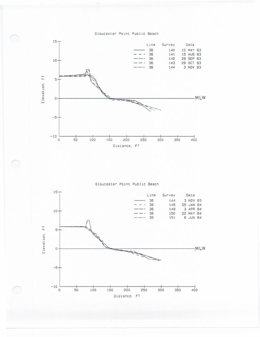
300 350 400

Gloucester Point PubliC 8each

15Line Survey Date

36 140 10 MAY8336 141 15 AUG 83

10+ 36 142 28 SEP 8336 143 29 OCT 83

I

36 144 3 NOV83

-111I-u- 5

C0.

..../0>

01 . MLWQJ-UJ

Gloucester Point Public 8each

Line Survey Date

36 144 3 NOV 8336 145 25 JAN 8436 149 3 APR 8436 150 22 MAY 8436 151 6 JUN 84

I-u- 5

C0.

..../0>QJ 0 .MLW- 00.

UJ

-5

-10o 50 100 150 200 250

Distance. FT

300 350 400

-10o 50 100 150 200 250 300 350 400

D:stance. FT

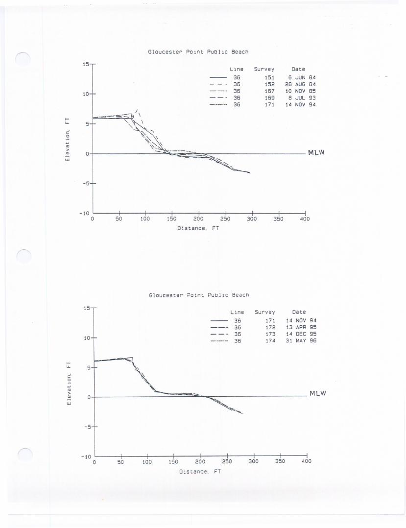
Gloucester ?oint PublIC 8eacn

15 .Line Survey Date

36 171 14 NOV 9436 172 13 APR 95

IOL

36 173 14 DEC 95-..--.- 36 174 31 MAY 96

u.. 5

C0

oWIt!

01> MLWQI-W I

.

I

......

-5

-5

-10o 50 100 150 200 250

Distance. FT

300 350 400

-10o 50 100 150 200 250

Distance. FT

300 350 400

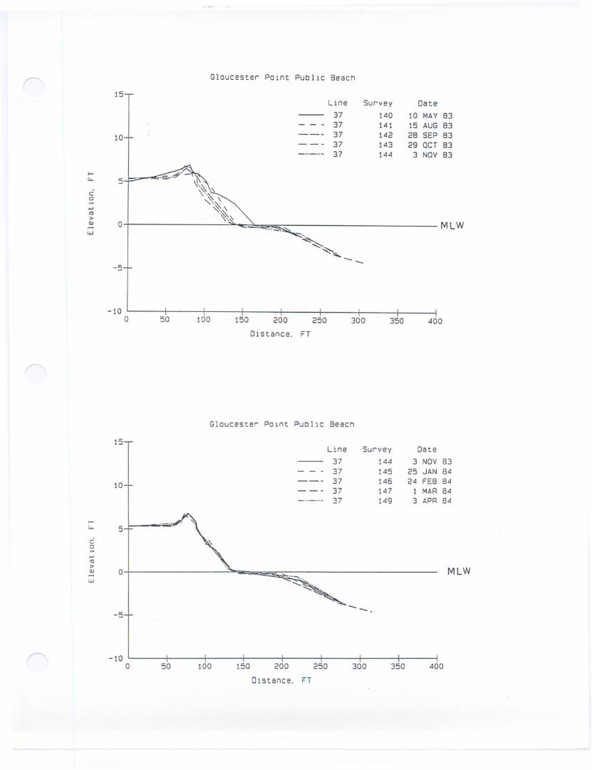
Gloucester Point Public Beach

15Line Survey Date

37 140 10 MAYB337 141 15 AUG 83

10+-"-"- 37 142 28 SEP 83

37 143 29 OCT 8337 144 3 NOV 83

II-u- 5C0.-...to>

MLWQ.I 01 --.........-w

-10o 50 100 150 200 250 300 350 400

Oistance. FT

Gloucester POlnt Public 8each

15

10

Line3737373737

Survey

167169171172173

Date

10 NOY 858 JUL 93

14 NOY 9413 APR 9514 DEC 95

co

MLW

I-u- 5

.oJftI>QI....W

o

\

-5

---10

o 50 100 150 200 250 300 350 400

Distance. FT

--- Gloucester Point Public 8each

15 .Line Survey Date

37 149 3 APR 8437 150 22 MAY 84

10+37 151 6 JUN 8437 152 28 AUG 84

L..-..-..

37 167 10 NOY 85

.{Q..I-u- 5

C0-.oJftI> MLWQI 0....w .

I

'.."

-5

-10o 50 100 150 200 250

Distance. FT

300 350 400

-5

-10o 50 100 150 200 250

Distance. FT

300 350 400

-5

-10o 50 100 150 200 250

Distance. FT

300 350 400

Gloucester Point Public 8each

15 _

Line Survey Date

39 140 10 MAY 8339 141 15 AUG 83

10+39 142 28 SEP 8339 143 29 OCT 83

I

39 144 3 NOV 83

-':...u- 5

C0-..10>

01 -QI MLW....

UJ

Gloucester Point Public 8each

15Line Survey Date

39 144 3 NOV 8339 145 25 JAN 84

10+ 39 149 3 APR 8439 150 22 MAY 8439 151 6 JUN 84

I _.,.u- 5

C0-..10>QI o I MLW....

-UJ

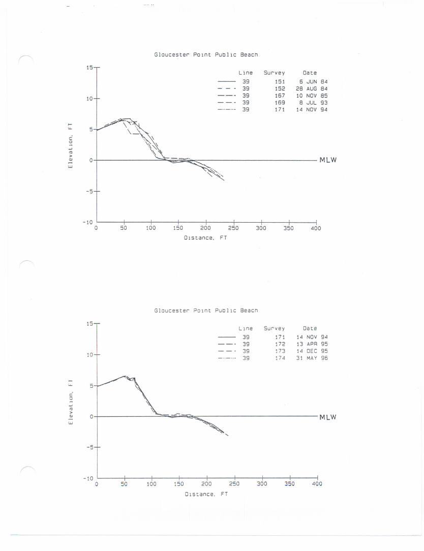
-5

-10o 50 100 150 200 250 300 350 400

Distance. FT

-10o 50 100 150 200 250 300 350 400

Dlstance. FT

Gloucester olnt PUOllC 8eacn

15Llne Survey Date

39 171 14 NOV 9439 172 13 APR 95

lor

39 173 14 DEC 95-..-..- 39 174 31 MAY 96

.....I.&.. 5

C0

-'<0>C1J 0 MLW-w '.::::!

..

I

"-

-5

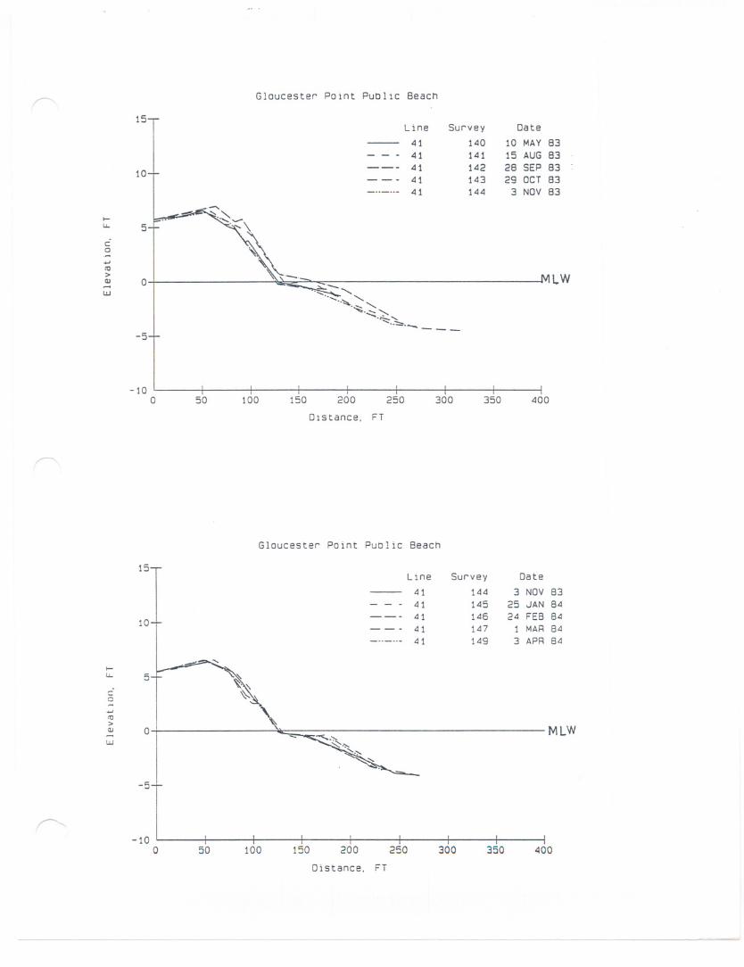
-10o 50 100 150 200 250 300 350 400

DIstance. FT

-5

-10o 50 100 150 200 250 300 350 400

Distance. FT

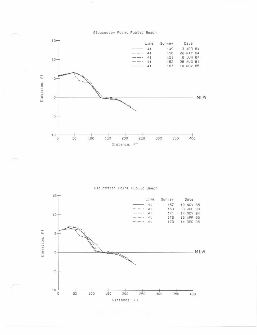
-5

-10o 50 100 150 200 250

Distance. FT

300 350 400

-5

-10o 50 100 150 200 250 300 350 400

Distance. FT

Gloucester POlnt PuOliC Beach

15Line Survey Date

41 167 10 NOV B541 169 B JUL 93

10+---- 41 171 14 NOV 94

41 172 13 APR 9541 173 14 DEC 95

I .....IJ.. 5

C0....It!>

o I 'b....-'--L - MLWQJ --w

.....

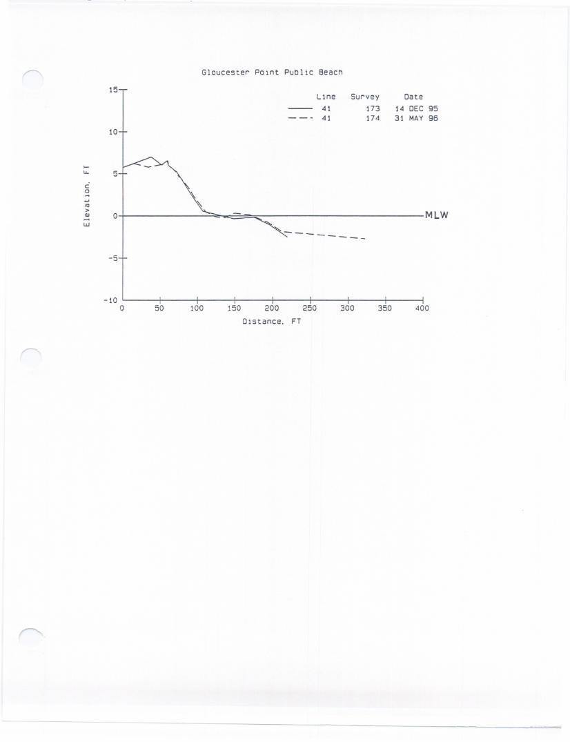
u. 5co.......<0>III~UJ

15

10

o

-5

-10o 50 100

Gloucester Point Public Beach

Line

41- - - 41

Survey

173174

'--------

150 200 250

Distance. FT

--

300

Date

14 DEC 9531 MAY 96

MLW

350 400

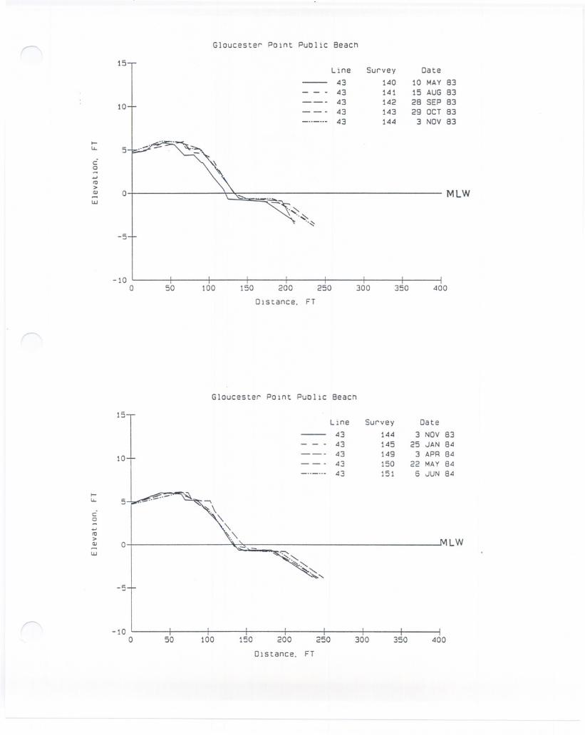
Gloucester Point Public Beach

15

10

Line4343434343

Survey

140141142143144

Date

10 MAY 83

15 AUG B328 SEP B329 OCT 83

3 NOV 83

co.-.wnJ>QJ....

UJMLW

~

u.. 5

o

-5

-10o 50 100 150 200 250 300 350 400

Distance. FT

15

10

-10o 50 100 150 200 250 300 350 400

Distance. FT

Gloucester POlnt Public Beach

Line Survey Date

43 144 3 NOV 8343 145 25 JAN 8443 149 3 APR B443 150 22 MAY 8443 151 6 JUN 84

5

LW

u.

c.0.w

-.

nJ>

0QJ

,

UJ

I-5

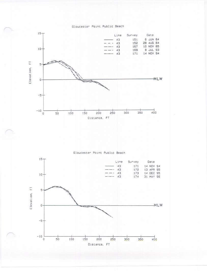
-5

-10o 50 100 150 200 250

Distance, FT

300 350 400

-5

---

-10o 50 100 150 200 250

Distance. FT

300 350 400

---- --- --

Gloucester Point PubliC 8eacn

15 ,Line Survey Date

43 151 6 JUN 8443 152 28 AUG 84

10+43 167 10 NOV 8543 169 8 JUL 93

I

43 171 14 NOV 94

-..-.-....u. 5

C0.....

..-

It)>

01 ,-OJ MLW-w

Gloucester Point Public 8eacn

15Line Survey Date

43 171 14 NOV 9443 172 13 APR 95

lor

43 173 14 DEC 95-...-...- 43 174 31 MAY 96

-....

u. 5

C0....

..-

It)>QJ 0 LW

"'-

w

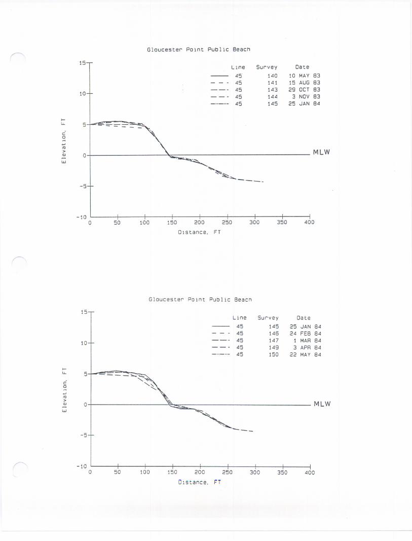
10

15

5 ~ --

MLW

c:

o-""'It!>QJ-UJ

o

......

~~:....._----5

-10o 50 100 150 200 250

Dlstance. FT

300 350 400

-----10

o 50 100 150 200 250

Olstance.n

300 350 400

Gloucester Point Public Beach

Line Survey Date

45 140 10 MAY 8345 141 15 AUG 8345 143 29 OCT 8345 144 3 NOV 8345 145 25 JAN 84

Gloucester POlnt PubliC Beach

15Line Survey Date

45 145 25 JAN 8445 146 24 FEB 84

10+ 45 147 1 MAR 8445 149 3 APR 8445 150 22 MAY 84

I

t-u- 5

C0--'It!>

MLWQJ 0UJ , ---

-5

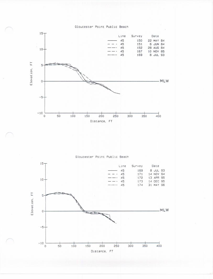
-5

-10o 50 100 150 200 250

Distance. FT

300 350 400

10

15

--

MLW

-5

-10o 50 100 150 200 250 300 350 400

Dlstance. FT

Gloucester Point PubliC Beacn

Line Survey Date

45 169 B JUL 9345 171 14 NOV 9445 172 13 APR 9545 173 14 DEC 9545 174 31 MAY 96

--u- 5

0....

ItI

>QJ 0-w

Gloucester Point PuOliC Beach

15

10

Line

4747474747

Survey

140141142143144

Date

10 MAY8315 AUG 8328 SEP 8329 OCT 83

3 NOV 83

-10o 150 200 250

Distance. FT

300 350 40050 100

-5

-10o 15050 100 200 250 300 350 400

Distance. FT

- - - - - - - - ----

I-5

MLW

u..

Ca-....

'.

10

'

>0

" §::'"

QI

".

....w

I-5

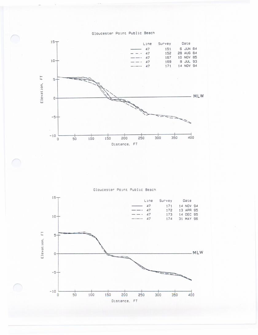
Gloucester Point Public Beach

15

10

Line

4747474747

Survey151152167169171

Date

6 JUN 8428 AUG 8410 NOV 85

8 JUL 9314 NOV 94

MLW

-5

.........

~~

"'>-'.c:::.''';'--==:':::':::'''~.~ "~

-10o 50 100 150 200 250

Distance. FT

300 350 400

I-u.. 5C0.-"-'10>Q) 0.....w

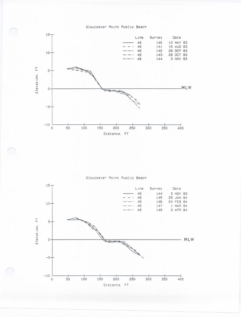
-10o 50 100 150 200 250

Distance. FT

300 350 400

-5

-10o 50 100 150 200 250 300 350 400

OlStance. FT

Gloucester Point Public Beach

15Line Survey Date

49 140 10 MAY 8349 141 15 AUG 83

10+49 142 28 SEP 8349 143 29 OCT 8349 144 3 NOV 83

I

U- 5

C0.-.....<tI> MLWOJ 0-w

......::::'"""""

"-..:::-..

-5+ ""."

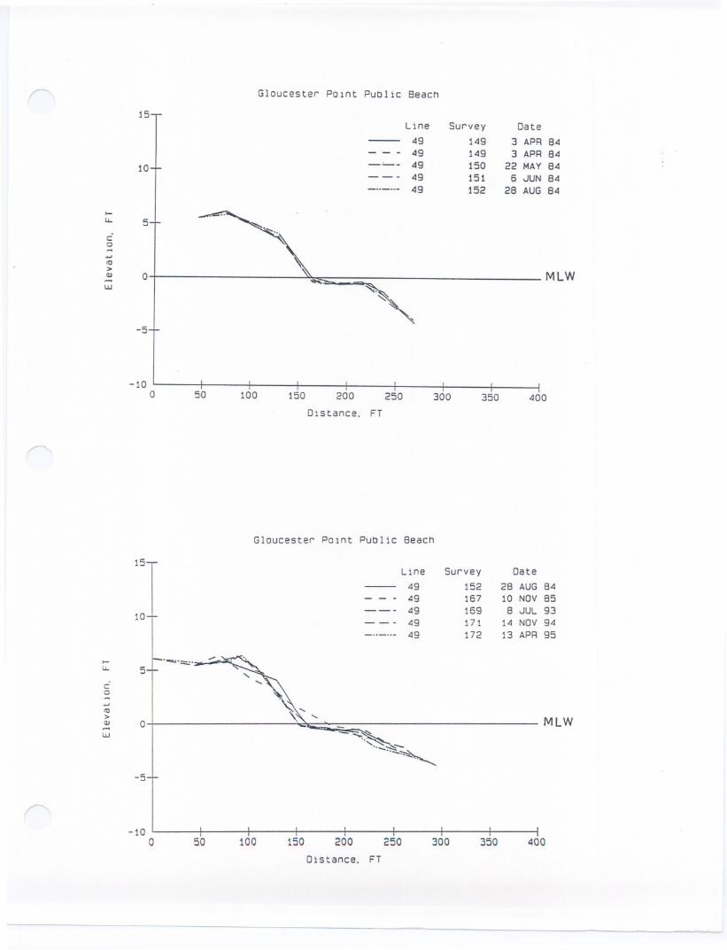
Gloucester Point Public 8each

15

10

Line4949494949

Survey149149150151152

Date

3 APR 843 APR 84

22 MAY 846 JUN 84

28 AUG 84

-5

-10o 50 100 150 200 250 300 350 400

Distance. FT

-10o 50 100 150 200 250 300 350 400

Distance. FT

0-u- 5C0.-....<0>

01cu '" MLW- -----w

Gloucester Point Public Beach

15

10

Line494949

Survey

172173174

Date

13 APR 9514 DEC 9531 MAY96

-5

-10o 50 100 150 200 250 300 350 400

Distance. FT

....u- 5C0.-....It!>

01'"QJ L MLW-

w

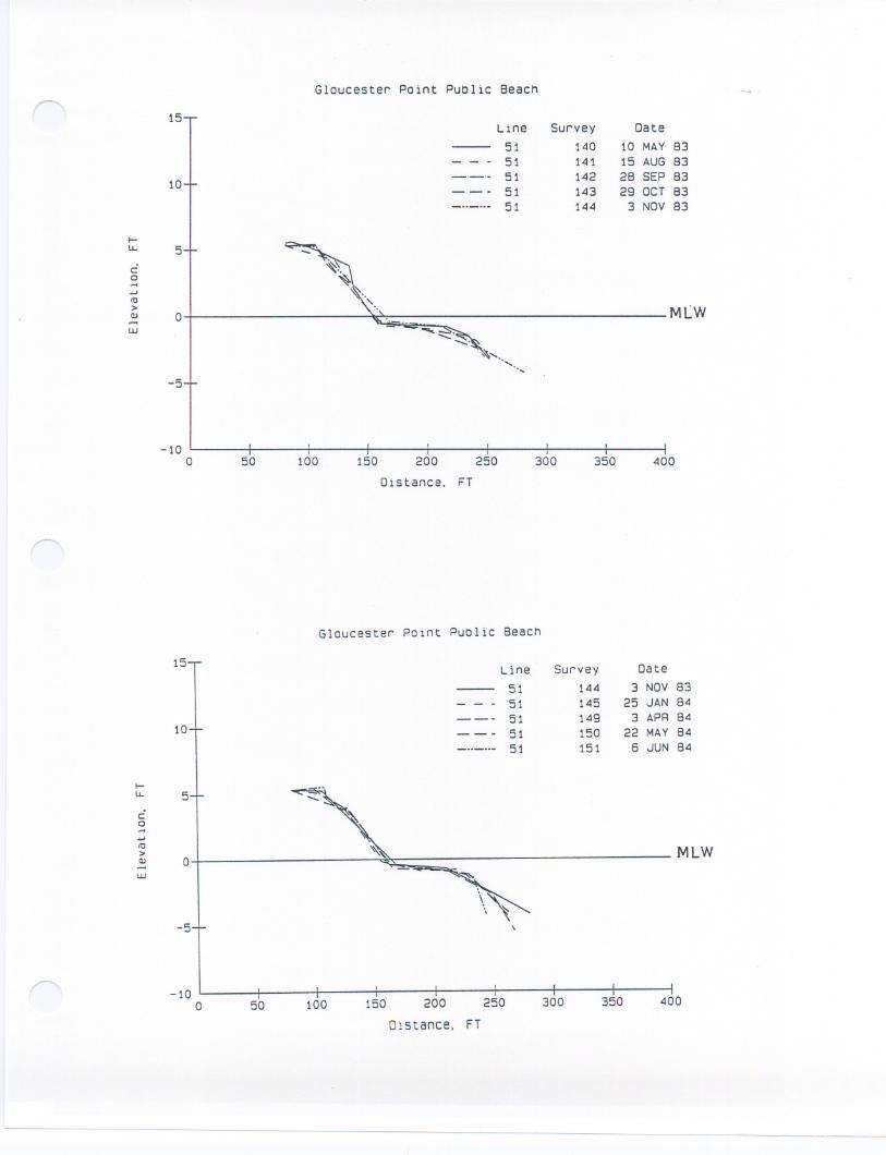
-5

-10o 50 100 150 200 250

Oistance. FT

300 350 400

-10o 50 100 150 200 250

Dlstance. FT

300 350 400

--- -------- -- -

Glouceste Point Public Beach

15Line Suvey Date

51 140 10 MAY 8351 141 15 AUG 83

10+51 142 28 SEP 8351 143 29 OCT 83

I

51 144 3 NOV 83

u. 5

C0....

"'-'

to>

01 "', MlWQJ- .

w

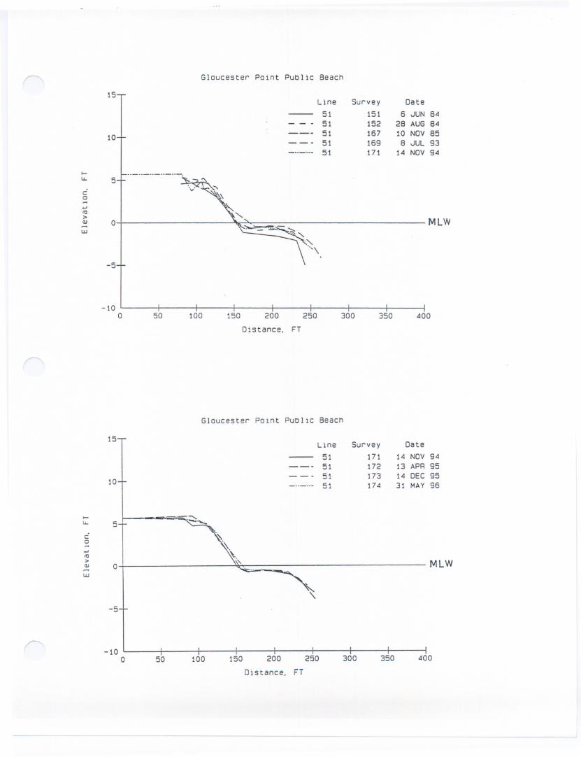
15

10

~

u.. 5Co.~

.w/0>CI.I.-W

o MLW

-5

-10o 50 100 150 200 250 300 350 400

Distance. FT

-5

-10o 50 100 150 200 250

Distance. FT

300 350 400

Gloucester Point PuDlic 8each

Line Survey Date

51 151 6 JUN 8451 152 28 AUG 8451 167 10 NOV 8551 169 8 JUL 9351 171 14 NOV 94

Gloucester Point PuDliC 8each

15 .Line Survey Date

51 171 14 NOV 9451 172 13 APR 95

lor

51 173 14 DEC 95-..-..- 51 174 31 MAY 96

u.. 5

C0

-'/0>

01 MLWCI.I

W

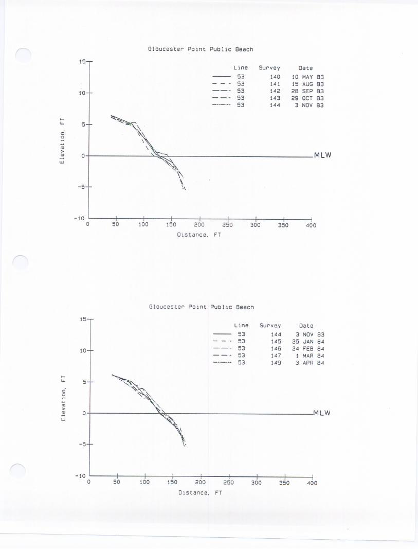
15

10

-10o 50 100 150 200 250

Distance. FT

300 350 400

-5

-10o 50 100 150 200 250 300 350 400

DIstance. FT

- ----- - --- - -------

Gloucester POInt Public Beach

Line Survey Date

53 140 10 MAY B353 141 15 AUG 8353 142 28 SEP 8353 143 29 OCT 8353 144 3 NOV 83

5'u. .

C0-.....

IQ>

01 ,.::--QJ MLW...

I.IJ

-5

Gloucester Point Public 8each

15Line Survey Date

53 144 3 NOV 8353 145 25 JAN 84

10+-.-- 53 146 24 FEB 84

53 147 1 MAR 8453 149 3 APR 84

I

u. 5C0

.....

IQ>

01,CI.I

"'....MLW

I.IJ

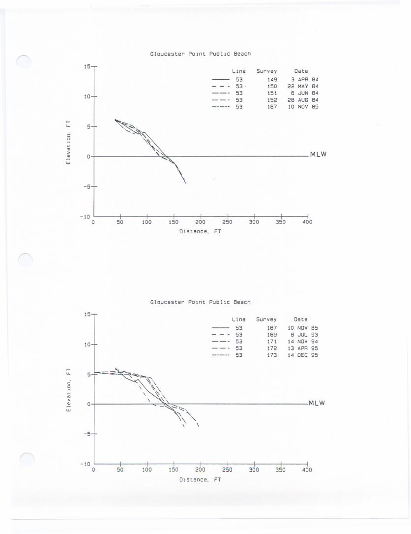
-10o

-5

50 250 400300 350100 150 200

Distance. FT

-10o

-5

50 150 400200 250 300100 350

Dlstance. FT

Gloucester Point PubliC Beach

15 _Line Survey Date

53 149 3 APR 8453 - 150 22 MAY84

10+53 151 6 JUN 8453 152 2B AUG 84

I

53 167 10 NOV85

.I-IJ.. 5C0-...It!>

01 ,. MLWQJ-UJ

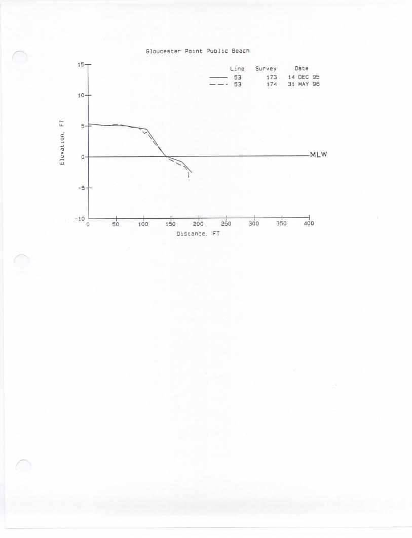
Gloucester Point Public Beach

15Line

53- - - 53

Survey173174

Date14 DEC9531 MAY96

10

-5

-10o 50 100 150 200 250

Distance. FT

300 350 400

....u.. 5C0.-....to>

01"-QJ MLW-0

UJ

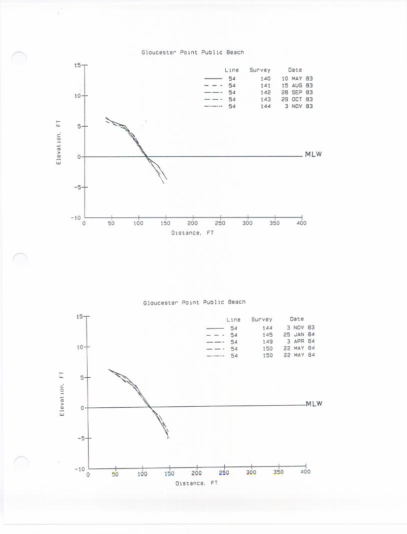
-5

-10o 50 150 200 250

Distance. FT

400300 350100

----

Gloucester Point Public 8each

15Line Survey Date

54 140 10 MAY 8354 141 15 AUG 83

10+54 142 28 SEP 8354 143 29 OCT 8354 144 3 Nav 83

I ....l-I.!.. 5

C0..../I)>

01 "- MLW(II-UJ

Gloucester POlnt Public 8each

15.-Line Survey Date

54 144 3 Nav 8354 145 25 JAN 84

10+54 149 3 APR 84

--- 54 150 22 MAY 84

I

54 150 22 MAY 84

........l-I.!.. 5

C0-.../I)

01 "\> MLW(II-UJ

-5-!- "

/' -

-10 -- I I

0 50 100 150 200 2;i0 300 350 400

Distance. FT

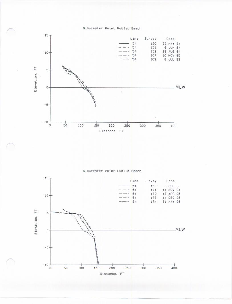
-10o

l-LL.

co.....10>Q.I....W

-10o

-5

50 100 150 200 250

DIstance. FT

300 350 400

Gloucester Point Public Beach

15

10

Line5454545454

Survey169171172173174

Date

8 JUL 9314 NDV 9413 APR 9514 DEC 9531 MAY96

5

MLWo

-5

50 150 200 250 300 350100 400

Distance. FT

--.. Gloucester Point Public Beach

15Line Survey Date

54 150 22 MAY B454 151 6 JUN B4

10+-"-"- 54 152 2B AUG 84

54 167 10 NDV 8554 169 8 JUL 93

Il-LL. 5

C0.........10>

o I '\\." MLWQ.I.... _\'-,

W

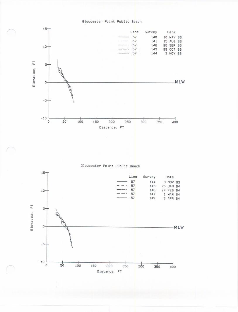
-5

-10o 50 100 150 200 250

Distance. FT

300 350 400

-5

-10o 50 100 150 200 250

Distance. FT

300 350 400

Gloucester Point Public 8each

15Line Survey Date

57 140 10 MAY8357 141 15 AUG 83

10+---- 57 142 28 SEP 83

57 143 29 OCT 8357 144 3 NOV 83

I I

IL. 5

C0

.....10>

01 '" f.1LWQI.....UJ

Gloucester Point Public 8each

15 ,Line Survey Date

57 144 3 NOV 8357 145 25 JAN 84

10+-.-.. 57 146 24 FE8 84

57 147 1 MAR8457 149 3 APR 84

I>-IL. 5

C0....10>

MLWQI o I ',UJ

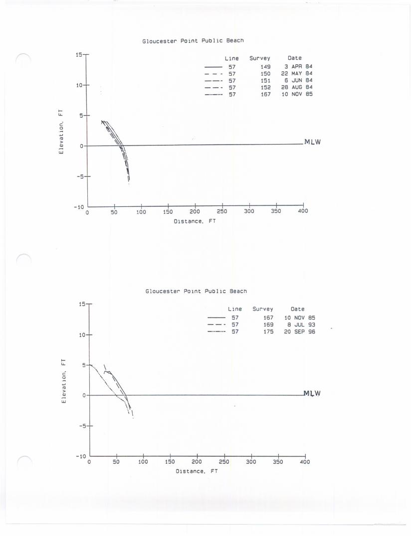
-5

-10o 50 100 150 200 250

Oistance. FT

300 350 400

Gloucester Point Public Beach

15

10

Line

575757

Survey167169175

Date

10 NOV 858 JUL 93

20 SEP 96

-5

-10o 50 100 150 200 250

Distance. FT

300 350 400

Gloucester Point Public Beach

15 ILine Survey Date

57 149 3 APR B457 150 22 MAYB4

10+57 151 6 JUN B457 152 28 AUG B4

I

57 167 10 NOV 85

I-U- 5

C0.....u/0

01 .> MLWQJ-UJ

I-51"-_, \

NJJ.,W

u-

c0....u

"', \\/0>

.. - &,QJ-UJ

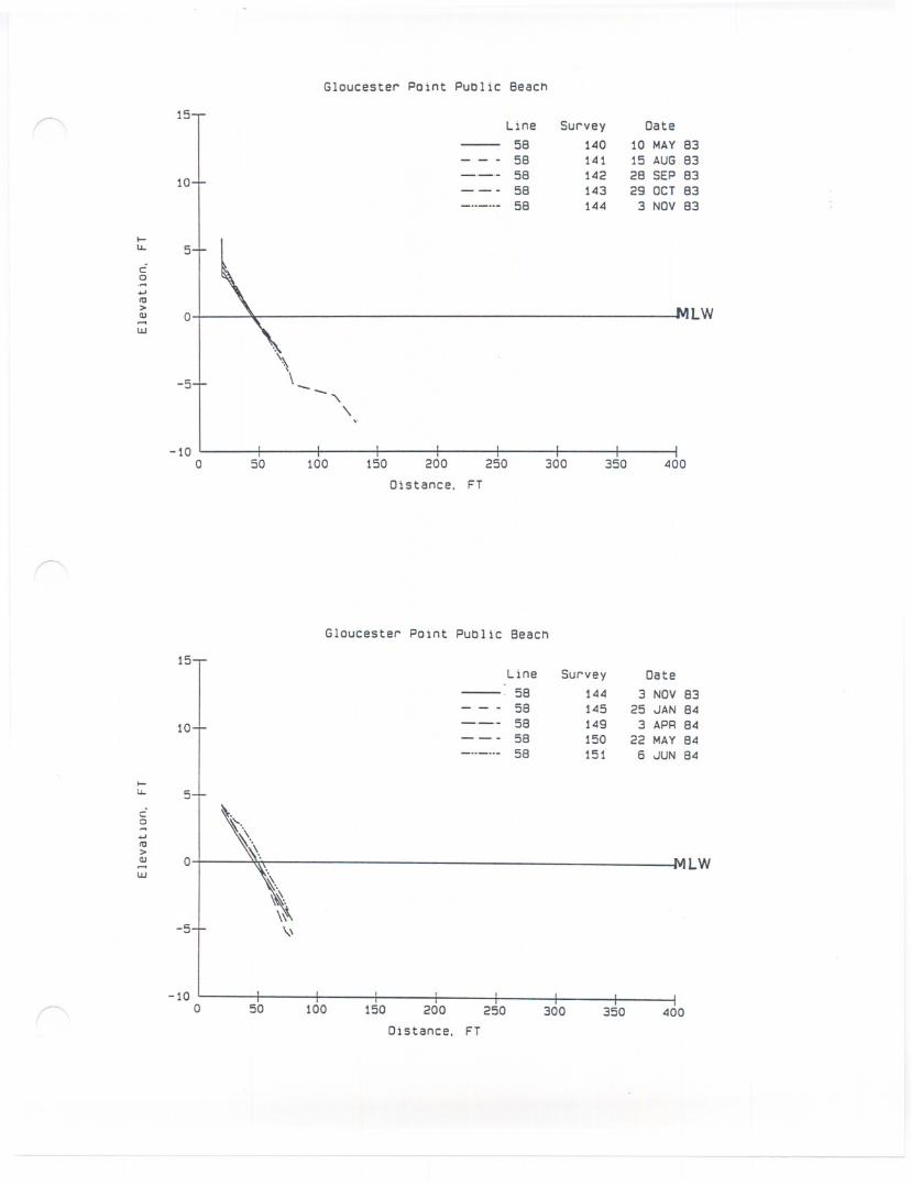
Gloucester Point Public Beach

15

10

Line

5858585858

Survey

144145149150151

Date

3 NOV 8325 JAN 84

3 APR 8422 MAY84

6 JUN 84

-10o 50 100 150 200 250

Distance. FT

300 350 400

.....u.. 5

.0- "....III ">QJ 0 \.-IJ.J .

"\.LW

-5+\'\\\

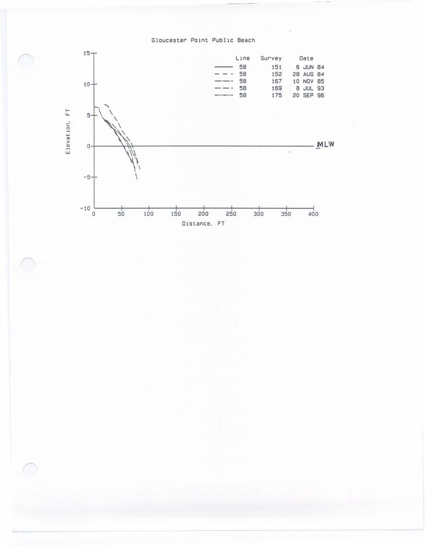
-5

-10o 150 200 250

Distance. FT

50 100 300 350 400

---- - - -