Embed Size (px)
Citation preview
Psych 230
Psychological Measurement and Statistics
Pedro Wolf
September 23, 2009
Correlation
Correlation
• Sometimes our research questions are concerned with finding the relationship between two variables
• Usually, these questions seek to observe these variables as they exist naturally in the world– the researcher is not trying to manipulate, but is
observing what occurs
• Often this type of research does not allow easy definition of ‘levels’ of the independent variable
Correlation
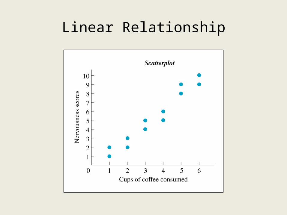
• Is coffee drinking related to nervousness?• Is sugar consumption related to hyperactivity in
children?• Are beer and coffee sales related to temperature?
• These type of questions are suited to a statistical technique known as correlation analysis
Statistical Testing
1. Decide which test to use2. State the hypotheses (H0 and H1)
3. Calculate the obtained value4. Calculate the critical value (size of )5. Make our conclusion
Statistical Testing
1. Decide which test to use2. State the hypotheses (H0 and H1)
3. Calculate the obtained value - calculate r4. Calculate the critical value (size of )5. Make our conclusion
Characteristics of Correlation Analyses - 1
• With correlational data, we don’t calculate a mean score for each condition– we don’t figure out mean beer sales in January,
February, March and so on
• Instead, the correlation coefficient [r] summarizes the entire relationship
Characteristics of Correlation Analyses - 2
• We always examine the relationship between pairs of scores– sugar consumption and hyperactivity– age and income– beer sales and temperature
• So, N is the number of pairs of scores in the data
Characteristics of Correlation Analyses - 3
• Neither variable is called the independent or dependent– sugar consumption and hyperactivity– age and income– beer sales and temperature
Characteristics of Correlation Analyses - 4
• We graph the scores differently in correlational research– we use a scatterplot to visualize our data
• A scatterplot is a graph that shows the location of each data point formed by a pair of X-Y scores
• When a relationship exists, a particular value of Y tends to be paired with one value of X and another value of Y tends to be paired with a different value of X
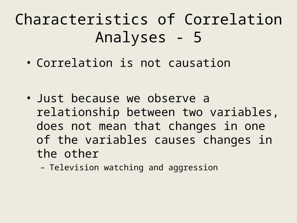
Characteristics of Correlation Analyses - 5
• Correlation is not causation
• Just because we observe a relationship between two variables, does not mean that changes in one of the variables causes changes in the other– Television watching and aggression
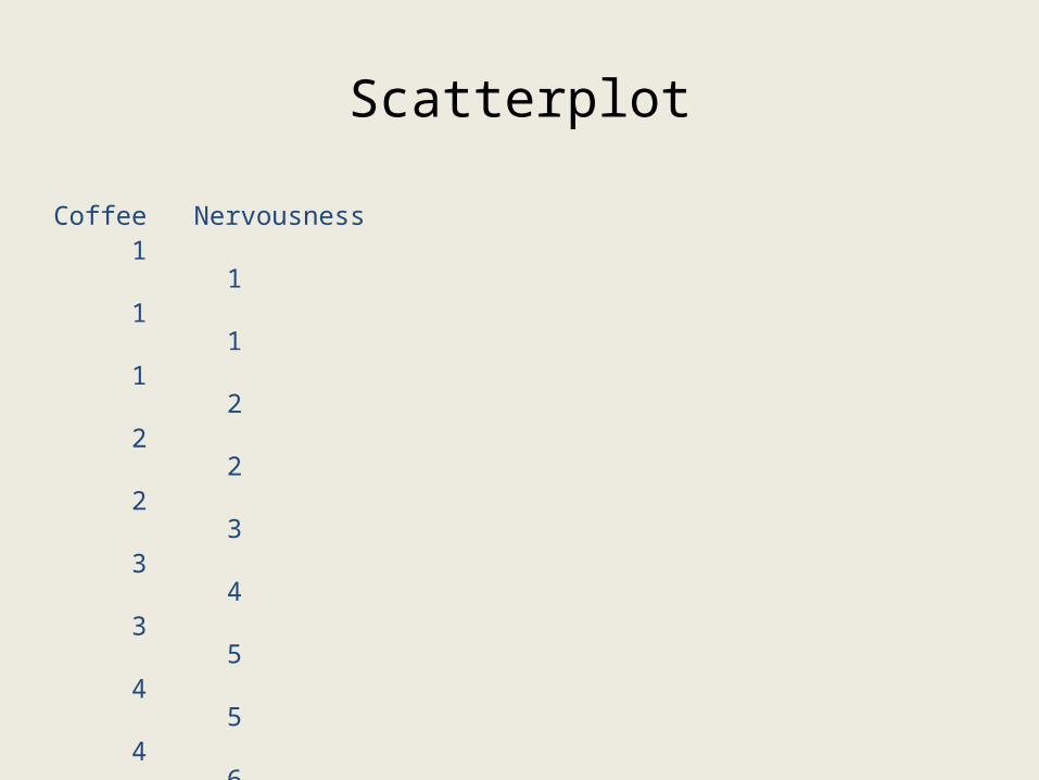
Scatterplot
Coffee Nervousness 1 1
1 1
1 2
2 2
2 3
3 4
3 5
4 5
4 6 5 8 5 9 6 9 6 10
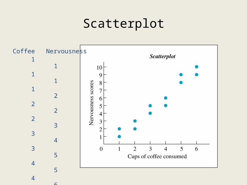
Scatterplot
Coffee Nervousness 1 1
1 1
1 2
2 2
2 3
3 4
3 5
4 5
4 6 5 8 5 9 6 9 6 10
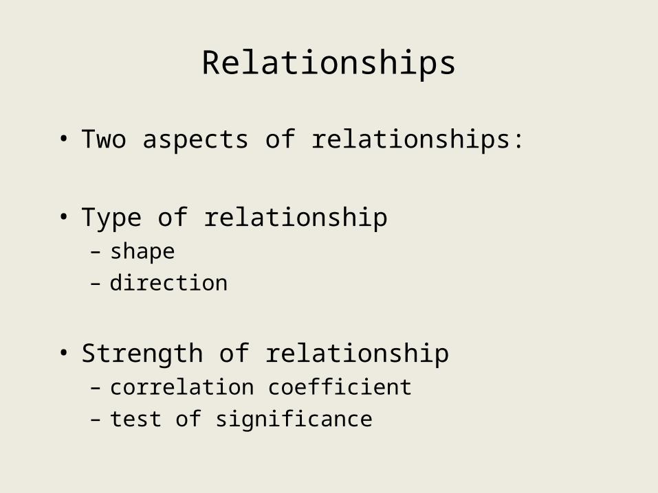
Relationships
• Two aspects of relationships:
• Type of relationship– shape – direction
• Strength of relationship– correlation coefficient– test of significance
Types of Relationship
• The type of relationship in a dataset can be thought of as the overall direction in which the scores on Y change as the X scores change – does knowing about variable 1 help you know something
about variable 2?
• There are two main types of relationship– Linear– Nonlinear
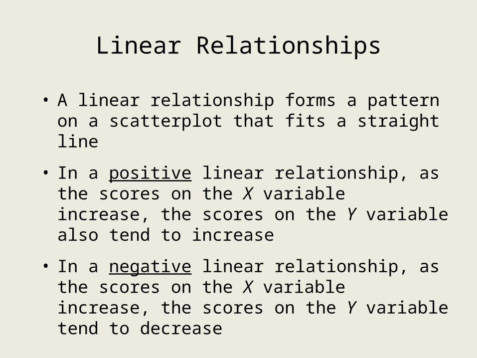
Linear Relationships
• A linear relationship forms a pattern on a scatterplot that fits a straight line
• In a positive linear relationship, as the scores on the X variable increase, the scores on the Y variable also tend to increase
• In a negative linear relationship, as the scores on the X variable increase, the scores on the Y variable tend to decrease
Linear Relationship
Linear Relationships
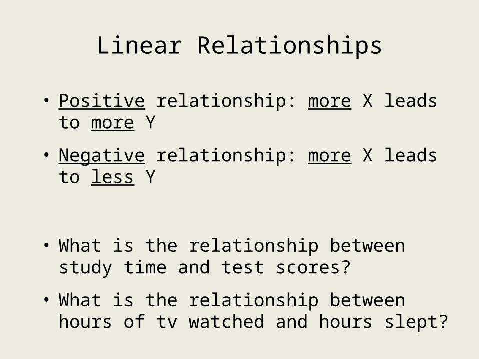
• Positive relationship: more X leads to more Y
• Negative relationship: more X leads to less Y
• What is the relationship between study time and test scores?
• What is the relationship between hours of tv watched and hours slept?
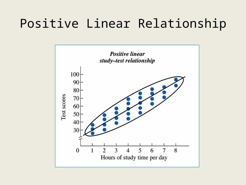
Positive Linear Relationship
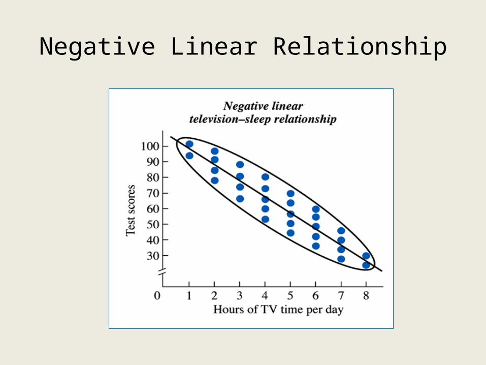
Negative Linear Relationship
Nonlinear Relationships
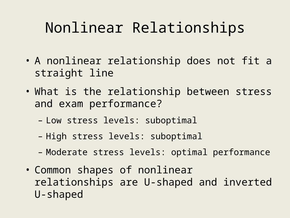
• A nonlinear relationship does not fit a straight line
• What is the relationship between stress and exam performance?
– Low stress levels: suboptimal
– High stress levels: suboptimal
– Moderate stress levels: optimal performance
• Common shapes of nonlinear relationships are U-shaped and inverted U-shaped
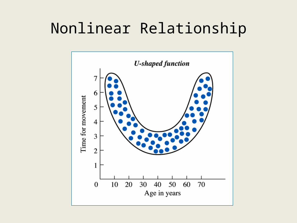
Nonlinear Relationship

Examples
1.X Y69 6663 7164 7065 7064 7562 7068 7274 6863 7265 75
2.X Y6 33 26 42 26 33 15 27 32 14 1
3.X Y40 330 2.610 3.215 3.840 3.745 2.850 3.420 215 3.325 3.8
4.X Y64 765 7.569 1063 7.564 765 1064 762 6.568 974 12
5.X Y20 525 1535 2040 3050 4555 4070 2080 2090 1095 10
65
66
67
68
69
70
71
72
73
74
75
76
60 62 64 66 68 70 72 74 76
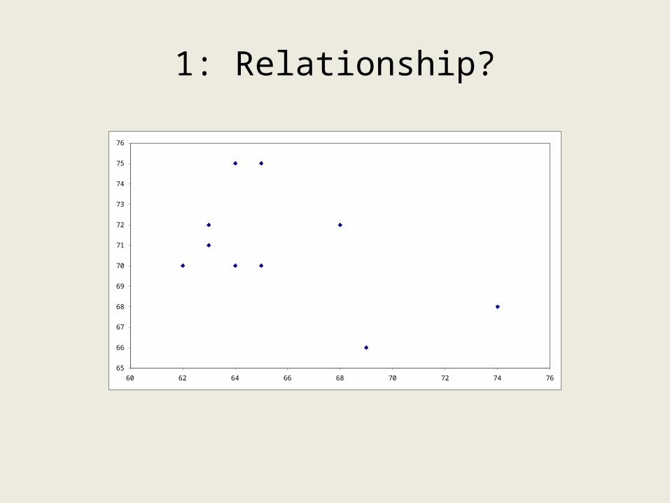
1: Relationship?
65
66
67
68
69
70
71
72
73
74
75
76
60 62 64 66 68 70 72 74 76
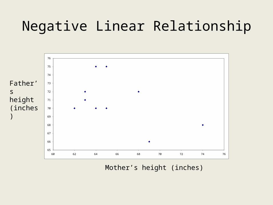
Negative Linear Relationship
Mother’s height (inches)
Father’s height (inches)
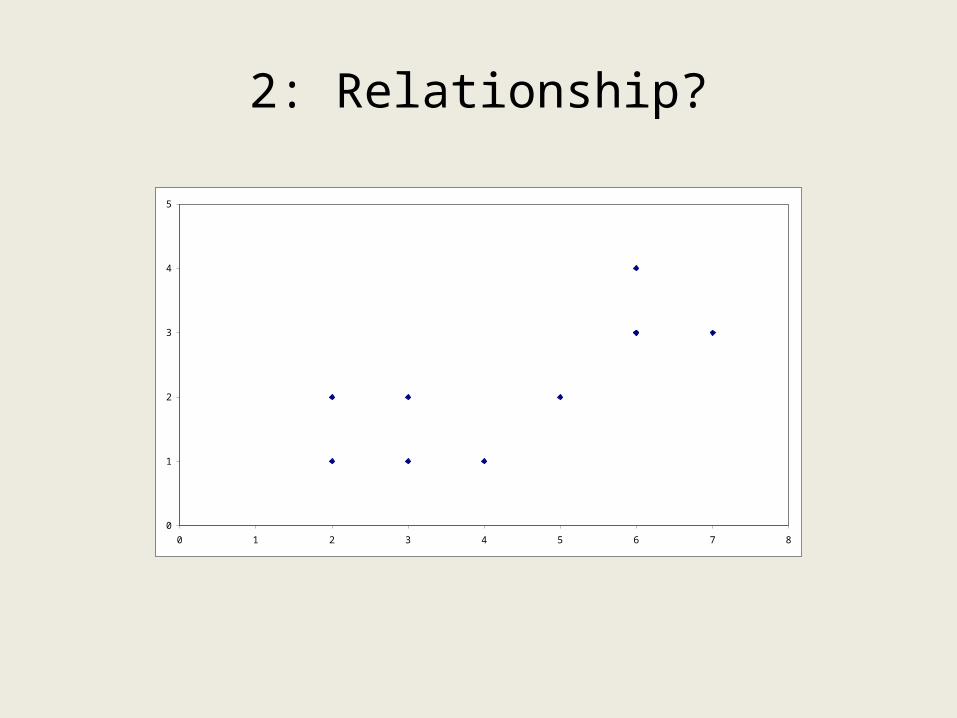
2: Relationship?
0
1
2
3
4
5
0 1 2 3 4 5 6 7 8
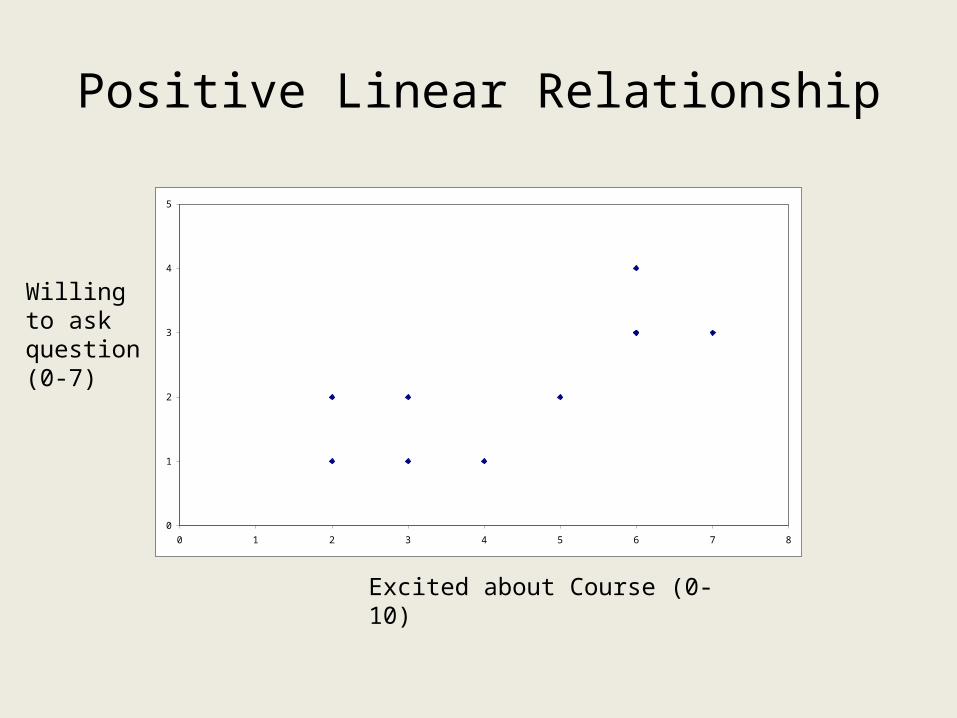
Positive Linear Relationship
0
1
2
3
4
5
0 1 2 3 4 5 6 7 8
Excited about Course (0-10)
Willing to ask question (0-7)
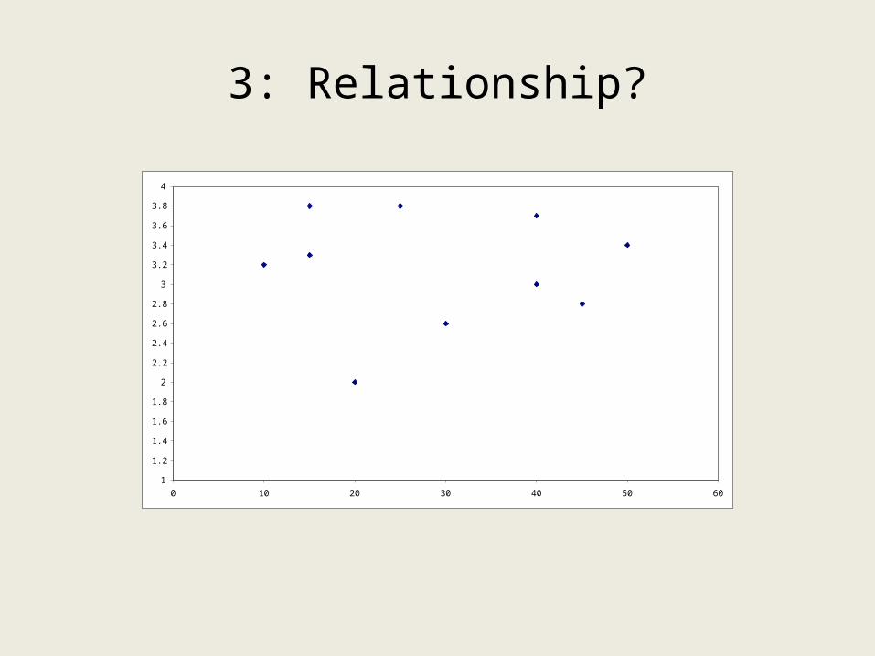
3: Relationship?
1
1.2
1.4
1.6
1.8
2
2.2
2.4
2.6
2.8
3
3.2
3.4
3.6
3.8
4
0 10 20 30 40 50 60
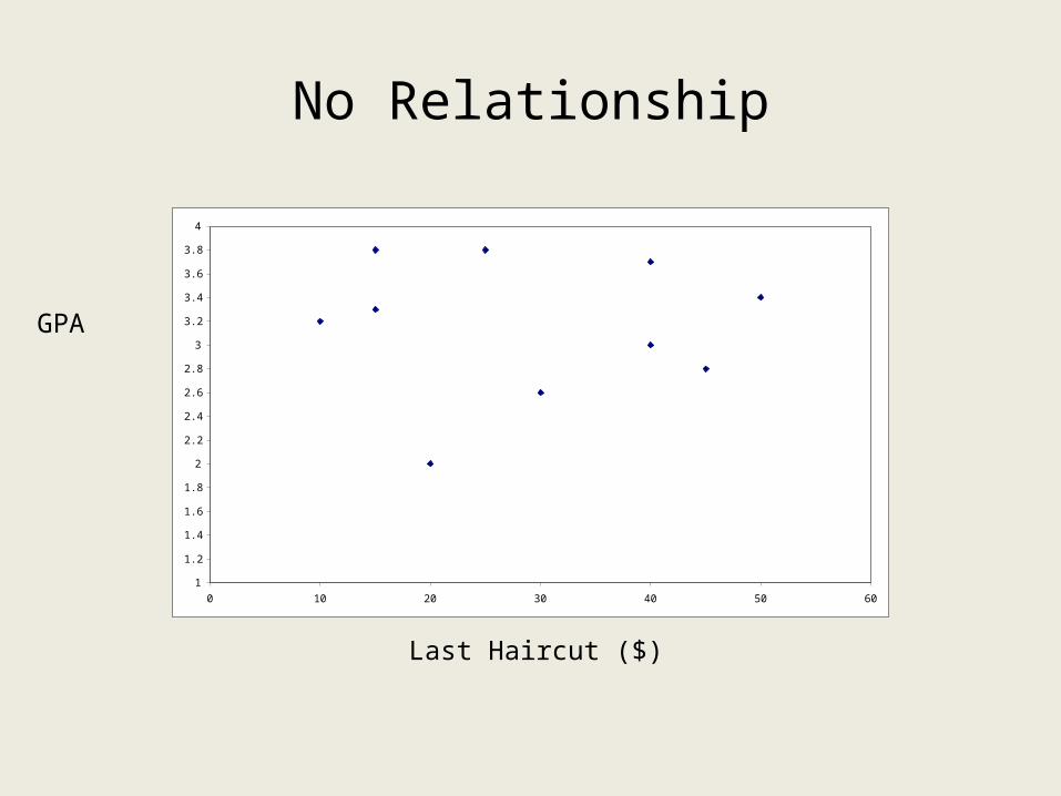
No Relationship
1
1.2
1.4
1.6
1.8
2
2.2
2.4
2.6
2.8
3
3.2
3.4
3.6
3.8
4
0 10 20 30 40 50 60
Last Haircut ($)
GPA
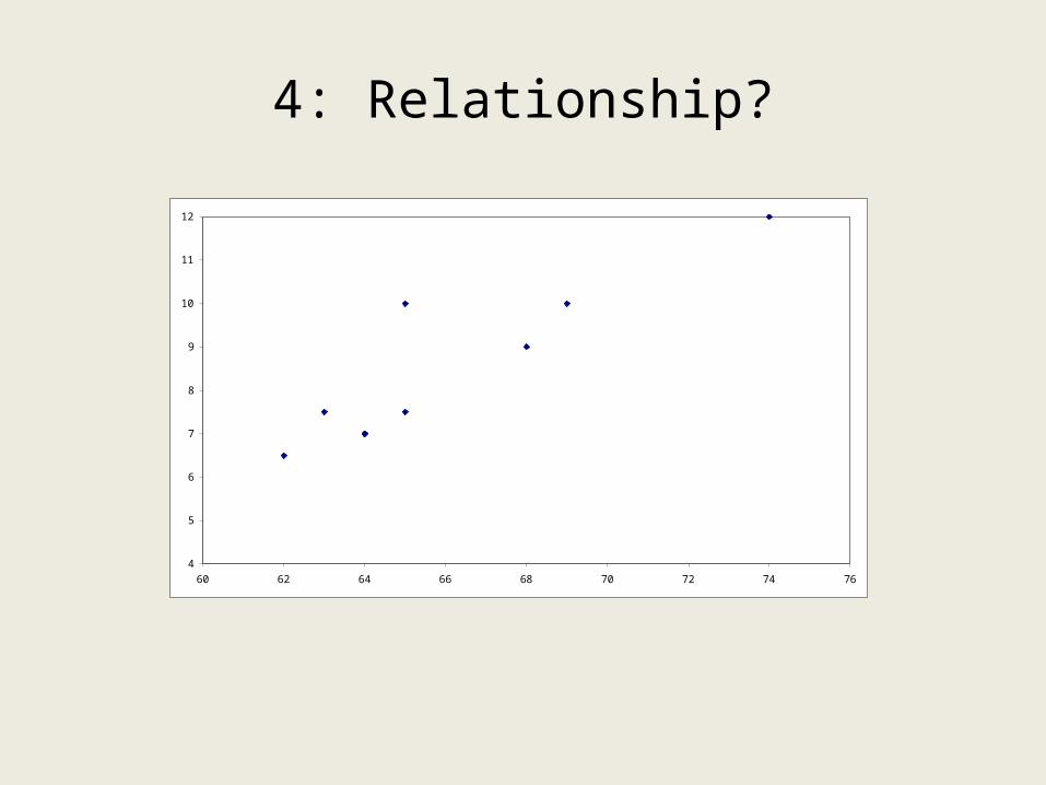
4: Relationship?
4
5
6
7
8
9
10
11
12
60 62 64 66 68 70 72 74 76
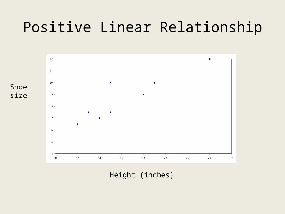
Positive Linear Relationship
4
5
6
7
8
9
10
11
12
60 62 64 66 68 70 72 74 76
Height (inches)
Shoe size
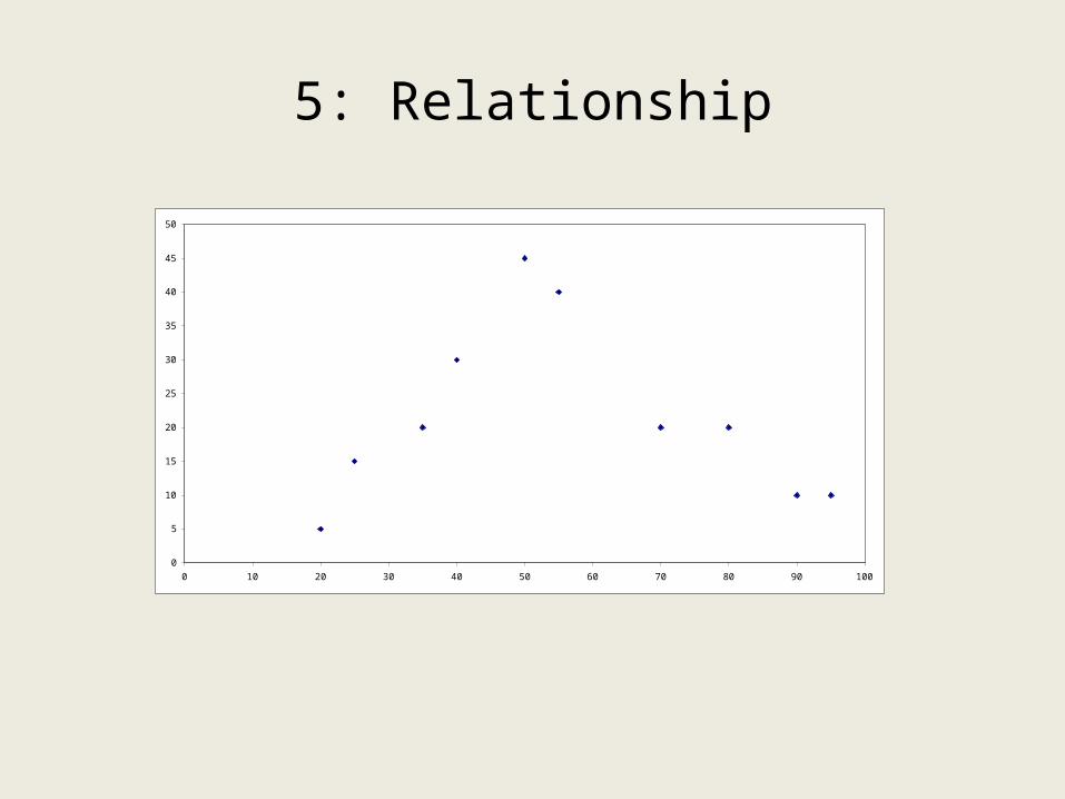
5: Relationship
0
5
10
15
20
25
30
35
40
45
50
0 10 20 30 40 50 60 70 80 90 100
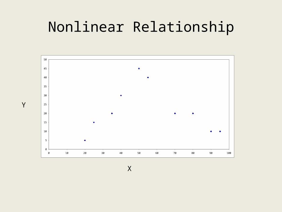
Nonlinear Relationship
X
0
5
10
15
20
25
30
35
40
45
50
0 10 20 30 40 50 60 70 80 90 100
Y
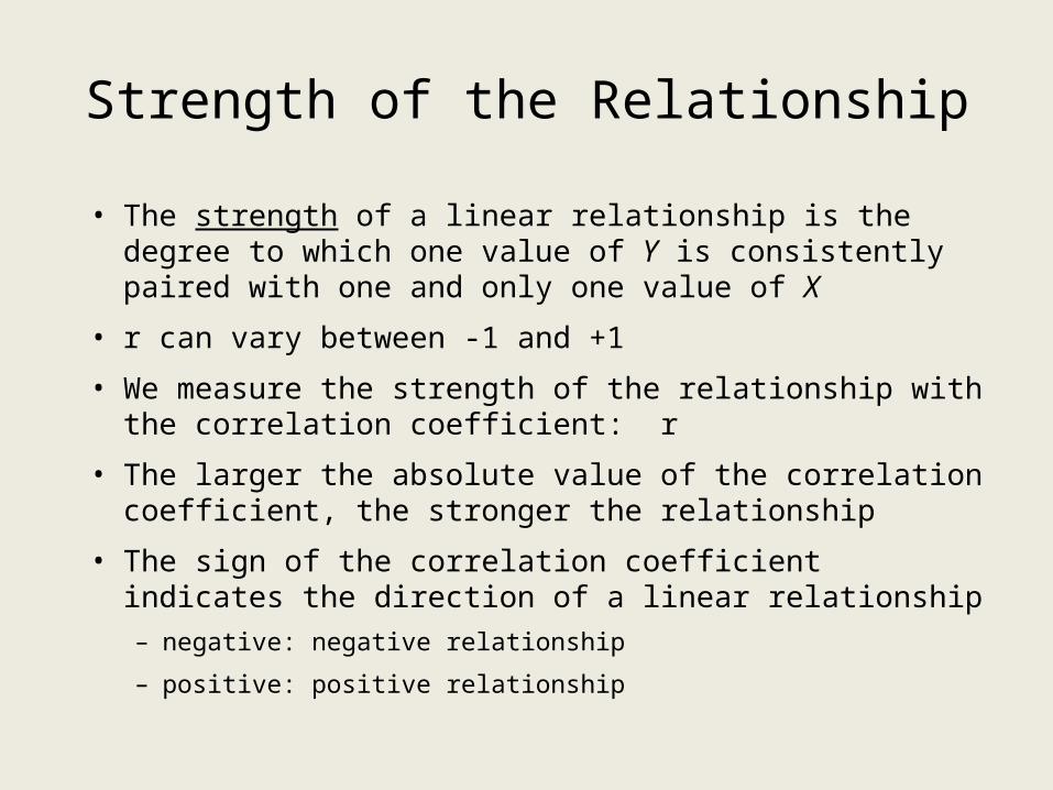
Strength of the Relationship
• The strength of a linear relationship is the degree to which one value of Y is consistently paired with one and only one value of X
• r can vary between -1 and +1
• We measure the strength of the relationship with the correlation coefficient: r
• The larger the absolute value of the correlation coefficient, the stronger the relationship
• The sign of the correlation coefficient indicates the direction of a linear relationship– negative: negative relationship
– positive: positive relationship
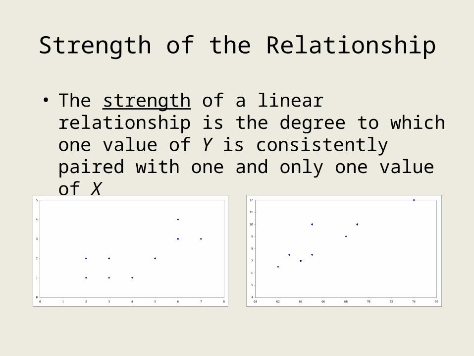
Strength of the Relationship
• The strength of a linear relationship is the degree to which one value of Y is consistently paired with one and only one value of X
0
1
2
3
4
5
0 1 2 3 4 5 6 7 8
4
5
6
7
8
9
10
11
12
60 62 64 66 68 70 72 74 76
Strength of the Relationship
• Describe the relationships between the variables which have the following correlations:
• A and B: R = 0.05
• C and D: R = -0.73
• E and F: R = 0.96
• G and H: R = 0.39
• I and J: R = -0.16
Strength of the Relationship
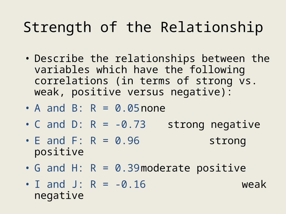
• Describe the relationships between the variables which have the following correlations (in terms of strong vs. weak, positive versus negative):
• A and B: R = 0.05 none
• C and D: R = -0.73 strong negative
• E and F: R = 0.96 strong positive
• G and H: R = 0.39 moderate positive
• I and J: R = -0.16 weak negative
Strength of the Relationship
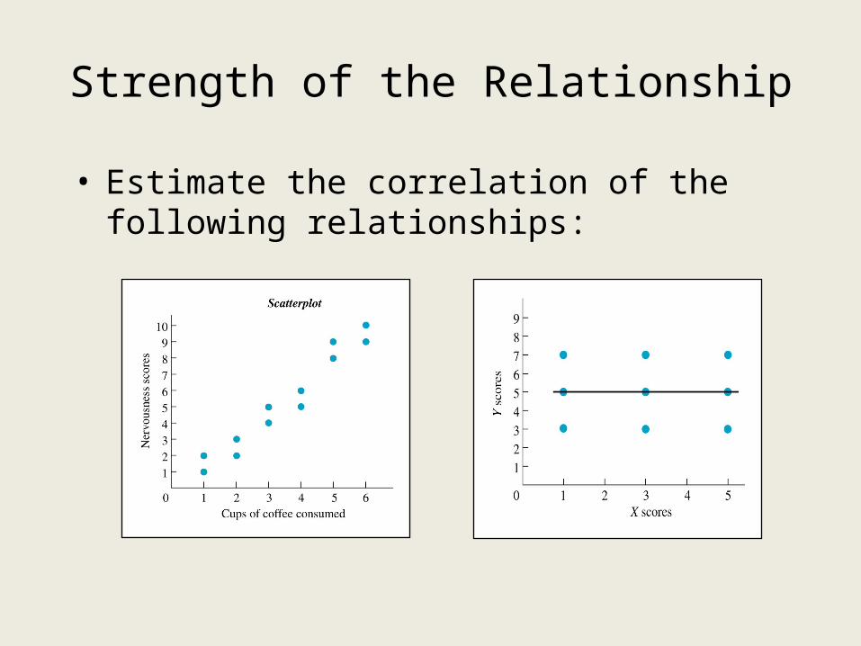
• Estimate the correlation of the following relationships:
Strength of the Relationship
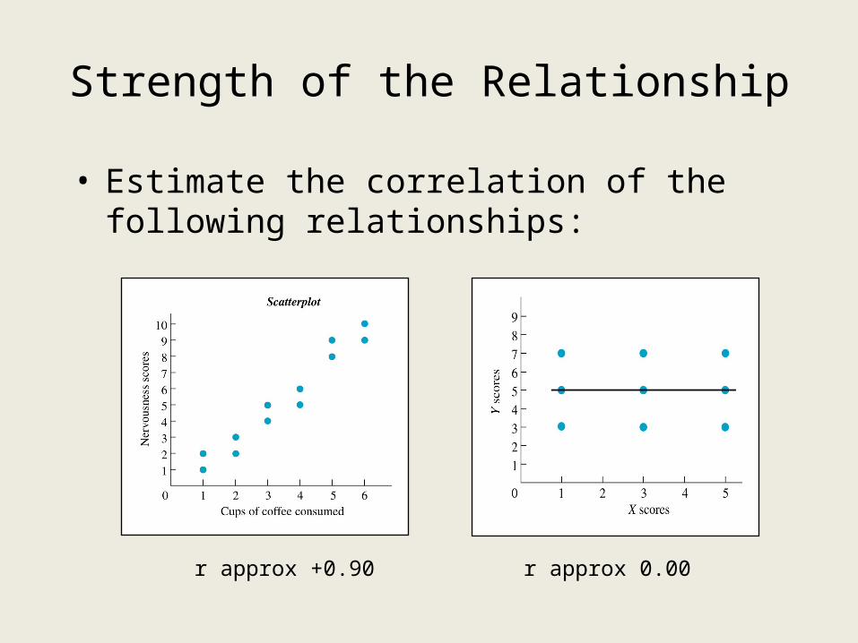
• Estimate the correlation of the following relationships:
r approx +0.90 r approx 0.00
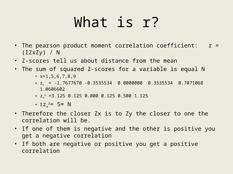
What is r?• The pearson product moment correlation coefficient: r = (ΣZxZy) /
N• Z-scores tell us about distance from the mean• The sum of squared Z-scores for a variable is equal N
• x=1,5,6,7,8,9• zx = -1.7677670 -0.3535534 0.0000000 0.3535534 0.7071068 1.0606602
• zx2 =3.125 0.125 0.000 0.125 0.500 1.125
• Σzx2= 5= N
• Therefore the closer Zx is to Zy the closer to one the correlation will be.• If one of them is negative and the other is positive you get a negative
correlation• If both are negative or positive you get a positive correlation
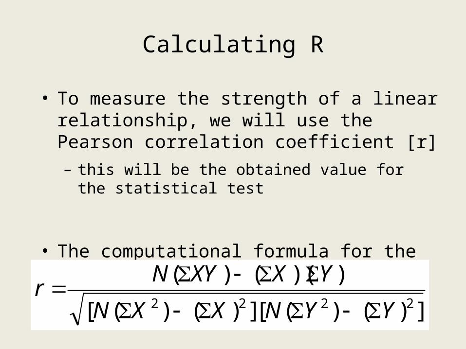
Calculating R
• To measure the strength of a linear relationship, we will use the Pearson correlation coefficient [r]– this will be the obtained value for the statistical test
• The computational formula for the correlation coefficient is:
])()([])()([
))(()(2222 YYNXXN
YXXYNr
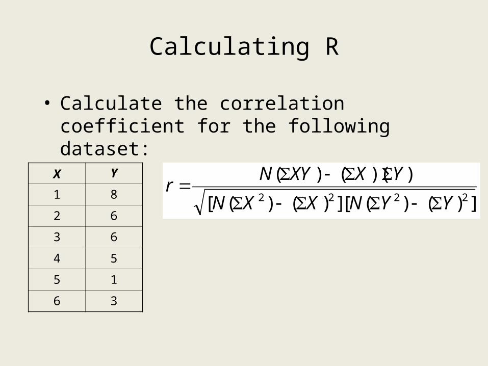
Calculating R
• Calculate the correlation coefficient for the following dataset:
])()([])()([
))(()(2222 YYNXXN
YXXYNr
X Y
1 8
2 6
3 6
4 5
5 1
6 3
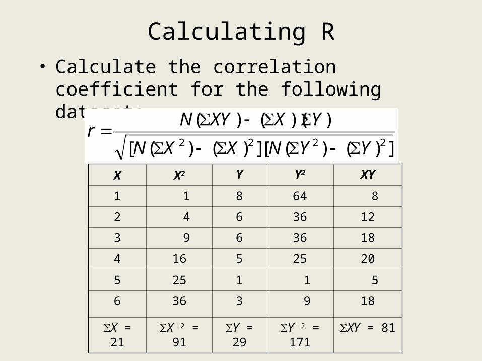
Calculating R• Calculate the correlation coefficient for the
following dataset:
X X2 Y Y2 XY
1 1 8 64 8
2 4 6 36 12
3 9 6 36 18
4 16 5 25 20
5 25 1 1 5
6 36 3 9 18
X = 21
X 2 = 91
Y = 29
Y 2 = 171
XY = 81
])()([])()([
))(()(2222 YYNXXN
YXXYNr
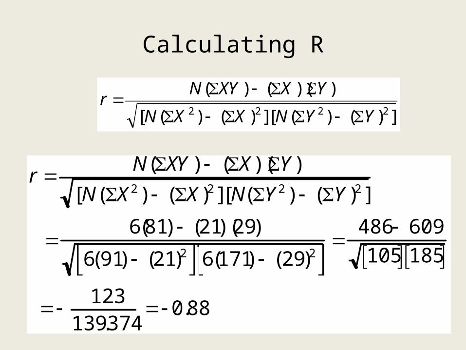
Calculating R
])()([])()([
))(()(2222 YYNXXN
YXXYNr
r N(XY ) (X)(Y )[N(X2 ) (X)2 ][N(Y 2 ) (Y )2 ]
6(81) (21)(29)
6(91) (21)2 6(171) (29)2 486 609105 185
123139.374
0.88
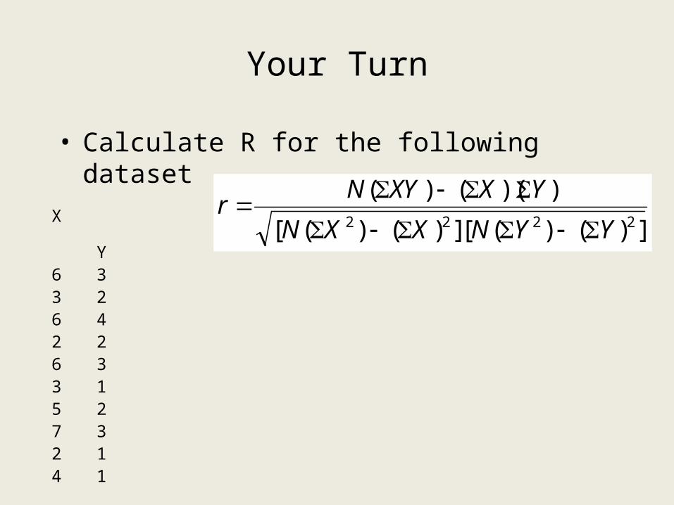
Your Turn
• Calculate R for the following dataset
X Y6 33 26 42 26 33 15 27 32 14 1
])()([])()([
))(()(2222 YYNXXN
YXXYNr
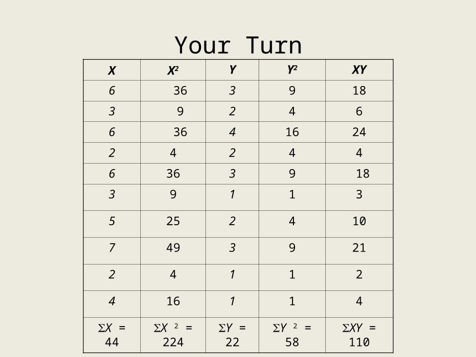
Your TurnX X2 Y Y2 XY
6 36 3 9 18
3 9 2 4 6
6 36 4 16 24
2 4 2 4 4
6 36 3 9 18
3 9 1 1 3
5 25 2 4 10
7 49 3 9 21
2 4 1 1 2
4 16 1 1 4
X = 44
X 2 = 224
Y = 22
Y 2 = 58 XY = 110
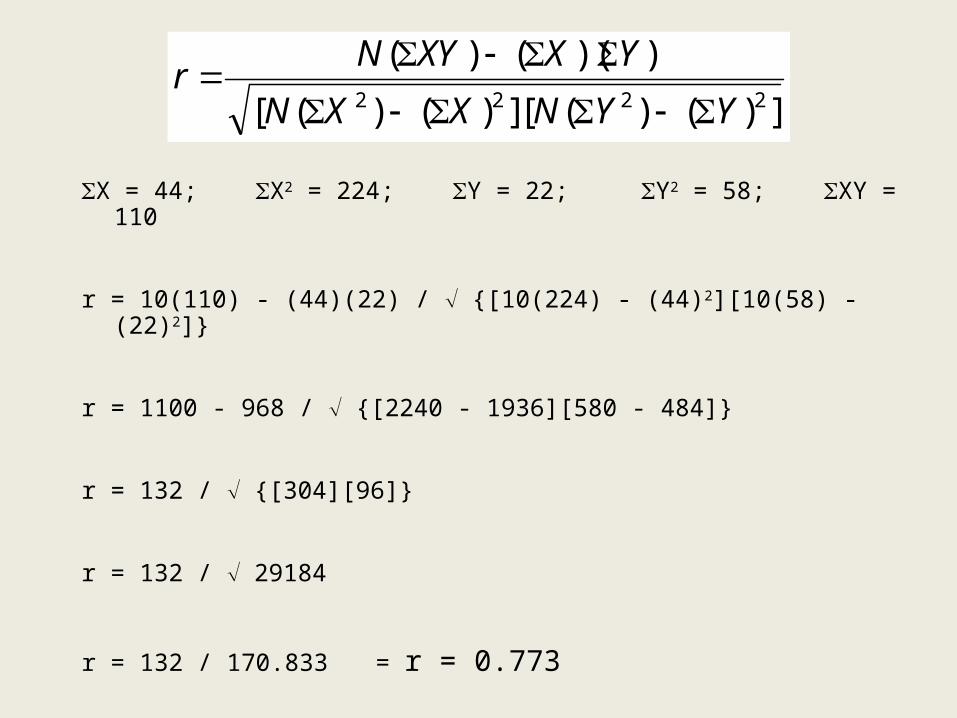
Your Turn
X = 44; X2 = 224; Y = 22; Y2 = 58; XY = 110
r = 10(110) - (44)(22) / {[10(224) - (44)2][10(58) - (22)2]}
r = 1100 - 968 / {[2240 - 1936][580 - 484]}
r = 132 / {[304][96]}
r = 132 / 29184
r = 132 / 170.833 = r = 0.773
])()([])()([
))(()(2222 YYNXXN
YXXYNr
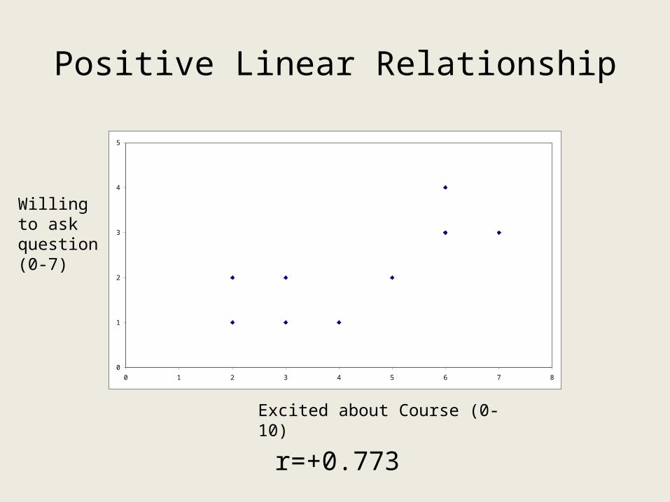
Positive Linear Relationship
0
1
2
3
4
5
0 1 2 3 4 5 6 7 8
Excited about Course (0-10)
Willing to ask question (0-7)
r=+0.773
Statistically testing correlations
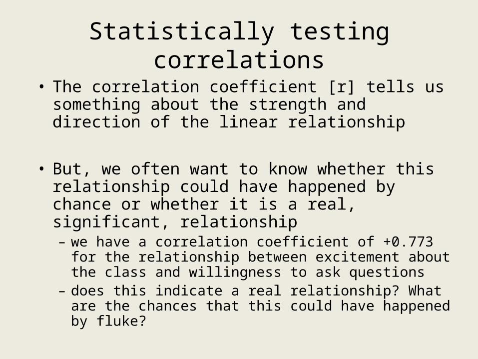
• The correlation coefficient [r] tells us something about the strength and direction of the linear relationship
• But, we often want to know whether this relationship could have happened by chance or whether it is a real, significant, relationship
– we have a correlation coefficient of +0.773 for the relationship between excitement about the class and willingness to ask questions
– does this indicate a real relationship? What are the chances that this could have happened by fluke?

Statistical Testing
1. Decide which test to use2. State the hypotheses (H0 and H1)
3. Calculate the obtained value4. Calculate the critical value (size of )5. Make our conclusion
Statistical Testing
1. Decide which test to use2. State the hypotheses (H0 and H1)
3. Calculate the obtained value - calculate r4. Calculate the critical value (size of )5. Make our conclusion

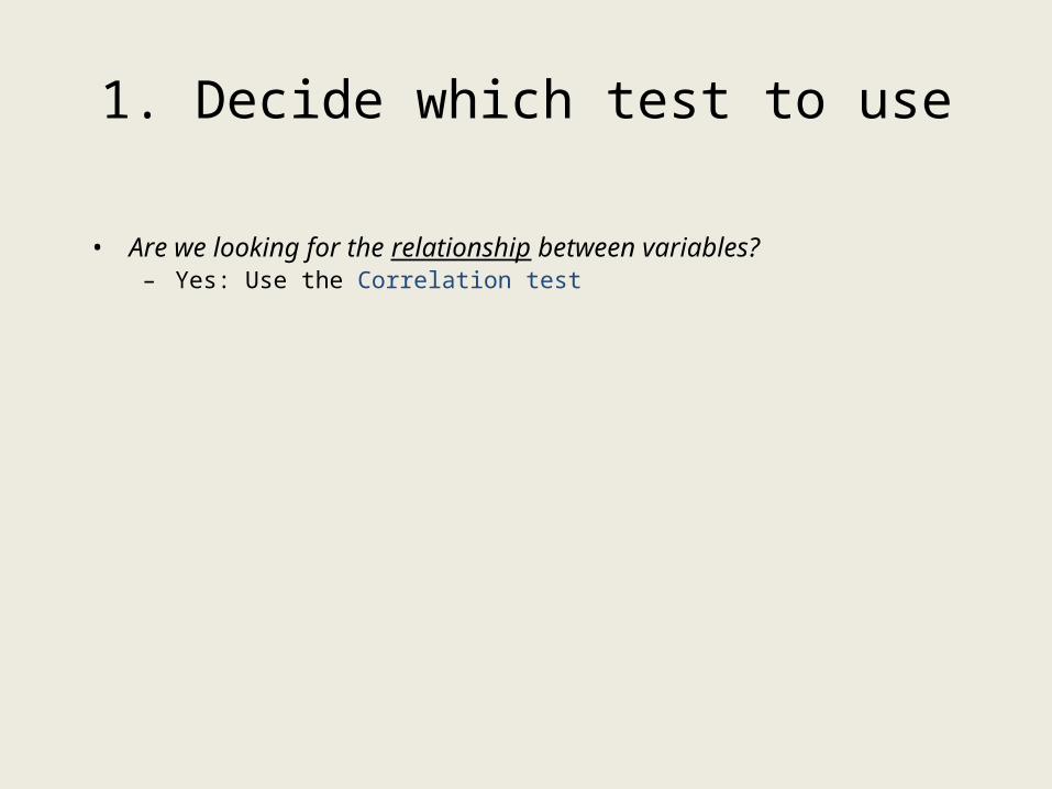
1. Decide which test to use
• Are we looking for the relationship between variables?– Yes: Use the Correlation test
2. State the Hypotheses
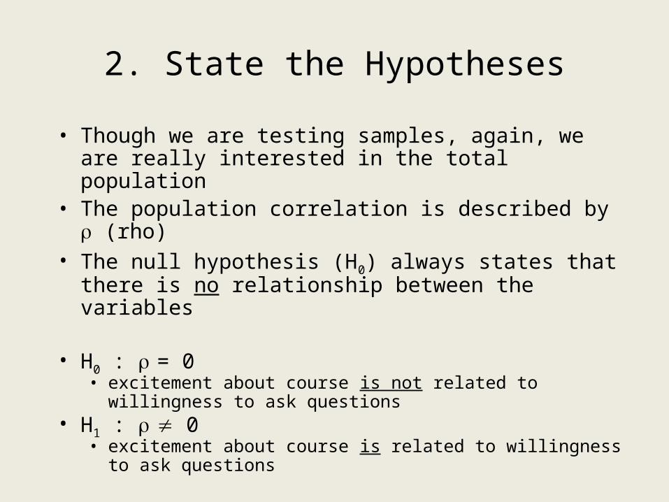
• Though we are testing samples, again, we are really interested in the total population
• The population correlation is described by (rho)• The null hypothesis (H0) always states that there is no
relationship between the variables
• H0 : = 0• excitement about course is not related to willingness to ask
questions • H1 : 0
• excitement about course is related to willingness to ask questions
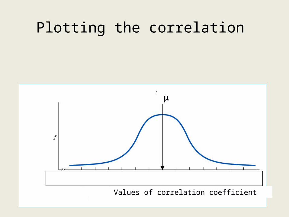
Plotting the correlation
a a a
a
Values of correlation coefficient

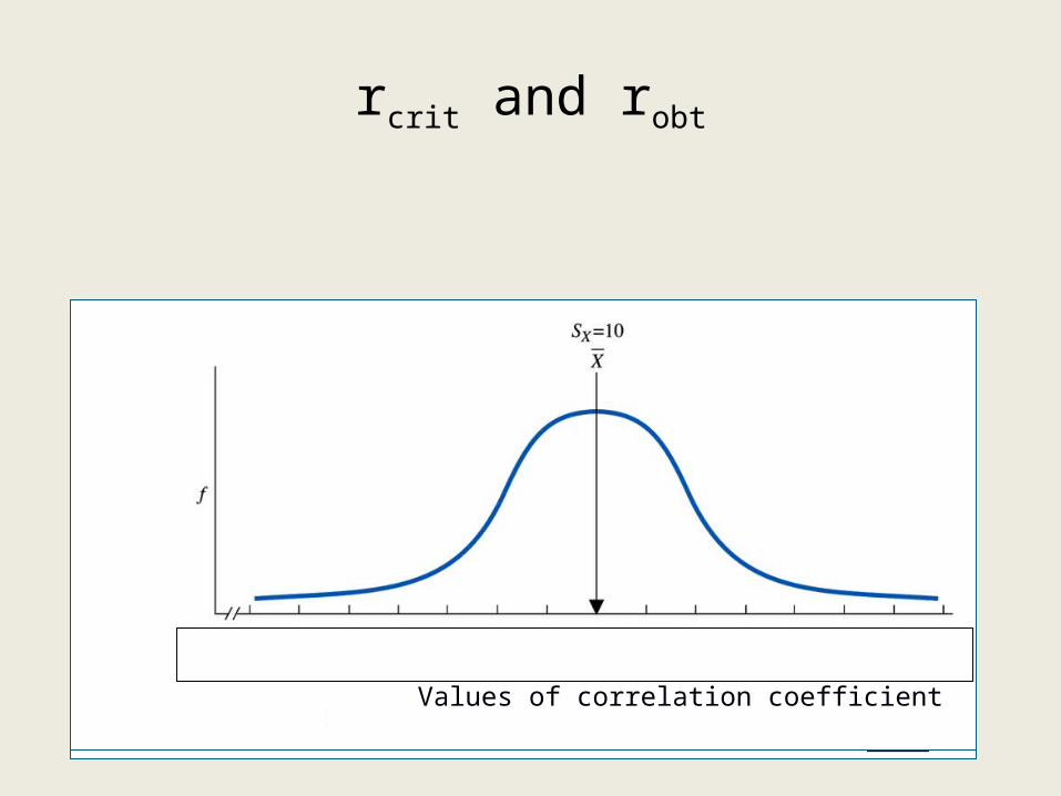
rcrit and robt
a
a a
a
rcrit=-0.67
robt=-0.78
Values of correlation coefficient
rcrit=+0.67
rcrit and robt
a a a
a
rcrit=-0.67
robt=+0.33
Values of correlation coefficient
rcrit=+0.67
Values of correlation coefficient
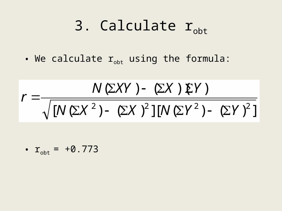
3. Calculate robt
• We calculate robt using the formula:
• robt = +0.773
])()([])()([
))(()(2222 YYNXXN
YXXYNr
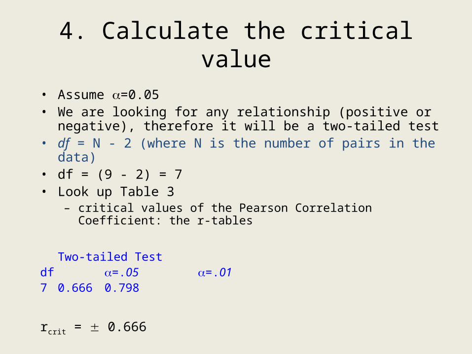
4. Calculate the critical value
• Assume =0.05• We are looking for any relationship (positive or negative), therefore it
will be a two-tailed test• df = N - 2 (where N is the number of pairs in the data) • df = (9 - 2) = 7• Look up Table 3
– critical values of the Pearson Correlation Coefficient: the r-tables
Two-tailed Testdf =.05 =.017 0.666 0.798
rcrit = 0.666
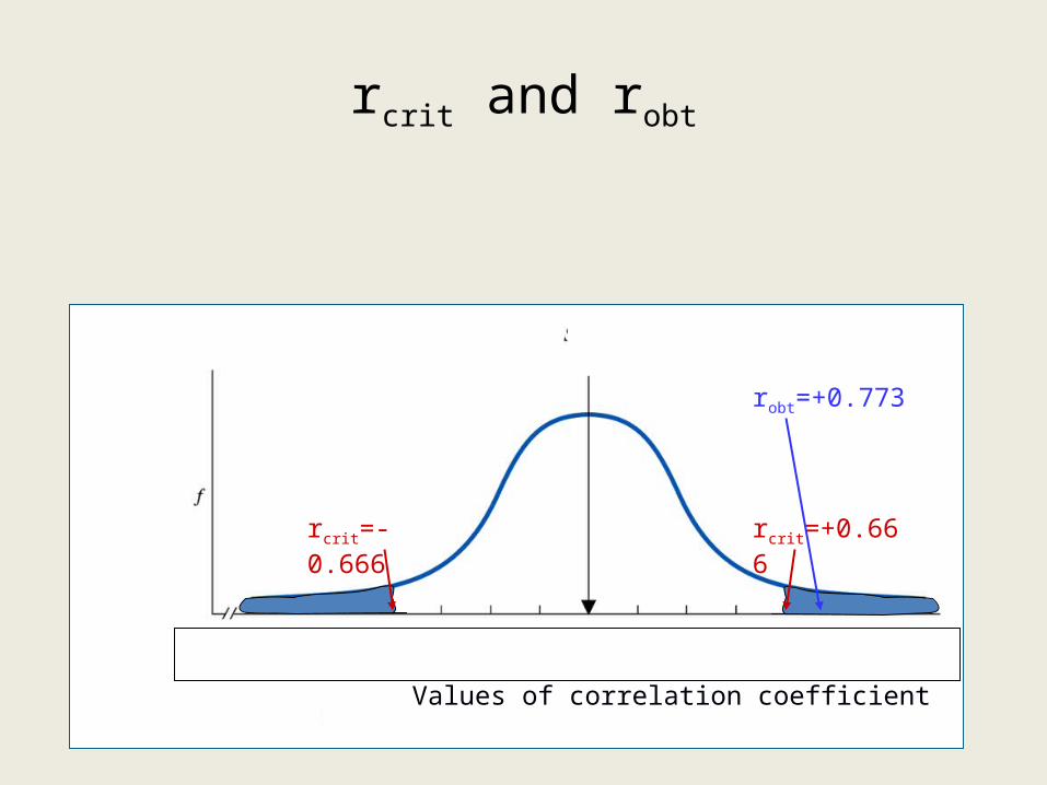
rcrit and robt
a a a
a
rcrit=-0.666
robt=+0.773
Values of correlation coefficient
rcrit=+0.666
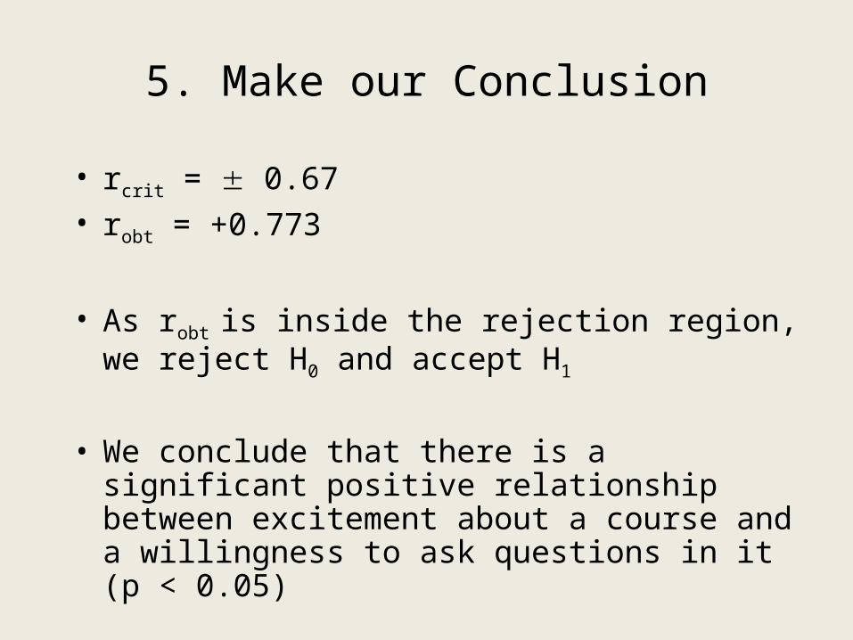
5. Make our Conclusion
• rcrit = 0.67• robt = +0.773
• As robt is inside the rejection region, we reject H0 and accept H1
• We conclude that there is a significant positive relationship between excitement about a course and a willingness to ask questions in it (p < 0.05)
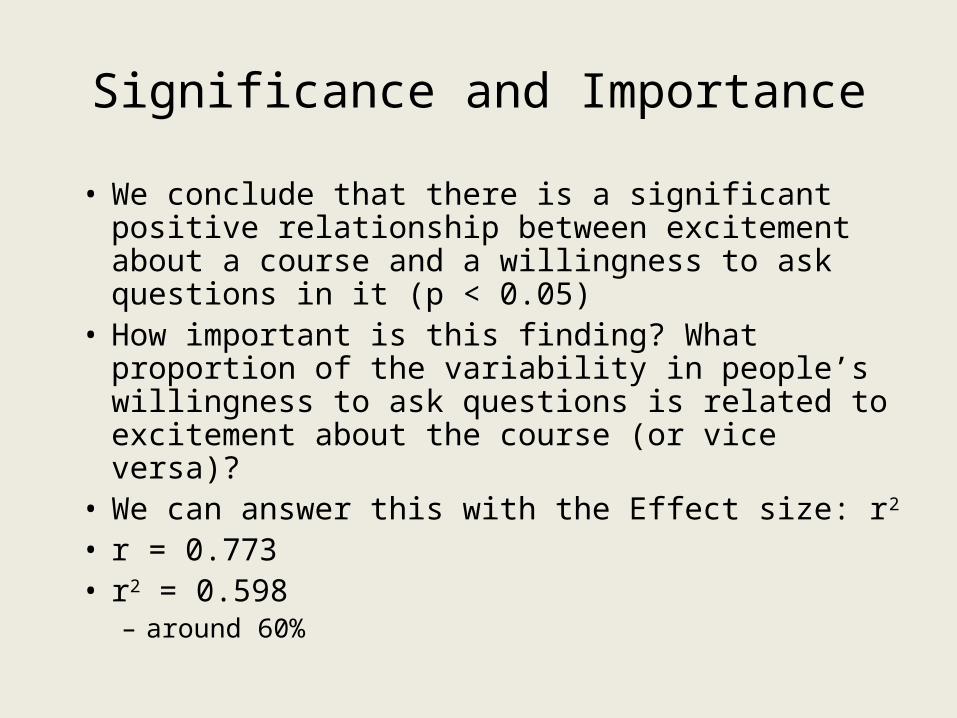
Significance and Importance
• We conclude that there is a significant positive relationship between excitement about a course and a willingness to ask questions in it (p < 0.05)
• How important is this finding? What proportion of the variability in people’s willingness to ask questions is related to excitement about the course (or vice versa)?
• We can answer this with the Effect size: r2
• r = 0.773• r2 = 0.598 – around 60%
Your Turn
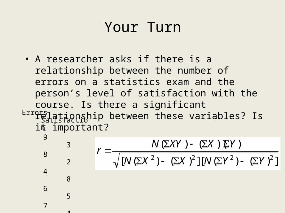
• A researcher asks if there is a relationship between the number of errors on a statistics exam and the person’s level of satisfaction with the course. Is there a significant relationship between these variables? Is it important?
Errors Satisfaction
9 3 8 2 4 8 6 5 7 4 10 2 5 7
])()([])()([
))(()(2222 YYNXXN
YXXYNr
1. Decide which test to use
• Are we looking for the relationship between variables?– Yes: Use the Correlation test
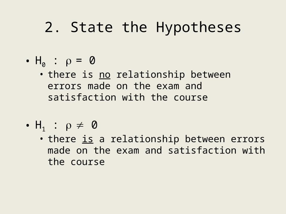
2. State the Hypotheses
• H0 : = 0• there is no relationship between errors made on the
exam and satisfaction with the course
• H1 : 0• there is a relationship between errors made on the exam
and satisfaction with the course
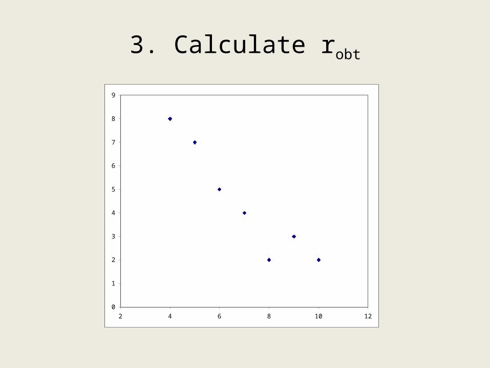
3. Calculate robt
0
1
2
3
4
5
6
7
8
9
2 4 6 8 10 12
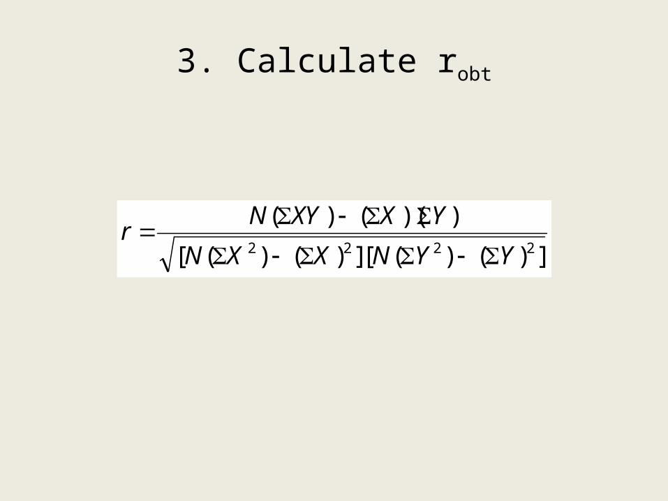
3. Calculate robt
])()([])()([
))(()(2222 YYNXXN
YXXYNr
3. Calculate robt
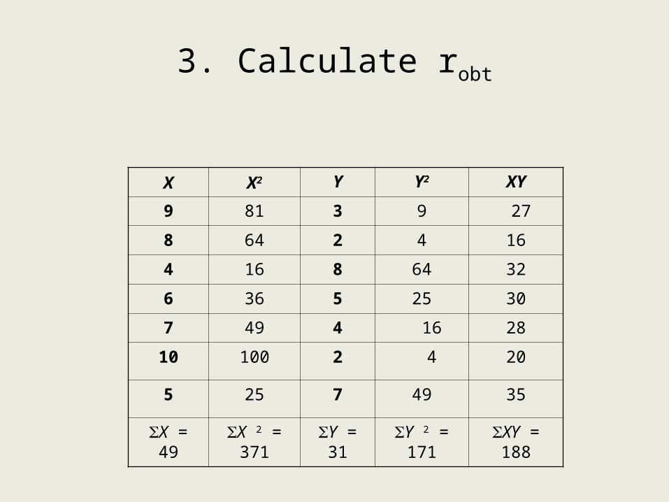
X X2 Y Y2 XY
9 81 3 9 27
8 64 2 4 16
4 16 8 64 32
6 36 5 25 30
7 49 4 16 28
10 100 2 4 20
5 25 7 49 35
X = 49
X 2 = 371
Y = 31
Y 2 = 171
XY = 188
Your Turn
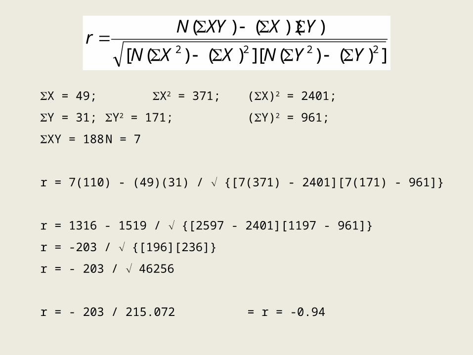
X = 49; X2 = 371; (X)2 = 2401;
Y = 31; Y2 = 171; (Y)2 = 961;
XY = 188 N = 7
r = 7(110) - (49)(31) / {[7(371) - 2401][7(171) - 961]}
r = 1316 - 1519 / {[2597 - 2401][1197 - 961]}
r = -203 / {[196][236]}
r = - 203 / 46256
r = - 203 / 215.072 = r = -0.94
])()([])()([
))(()(2222 YYNXXN
YXXYNr

4. Calculate the critical value
• Assume =0.05• We are looking for any relationship (positive or negative), therefore it
will be a two-tailed test• df = N - 2 (where N is the number of pairs in the data) • df = (7 - 2) = 5• Look up Table 3
– critical values of the Pearson Correlation Coefficient: the r-tables
Two-tailed Testdf =.05 =.015 0.754 0.874
rcrit = 0.754
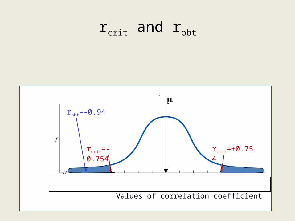
rcrit and robt
a a a
a
rcrit=-0.754
robt=-0.94
Values of correlation coefficient
rcrit=+0.754
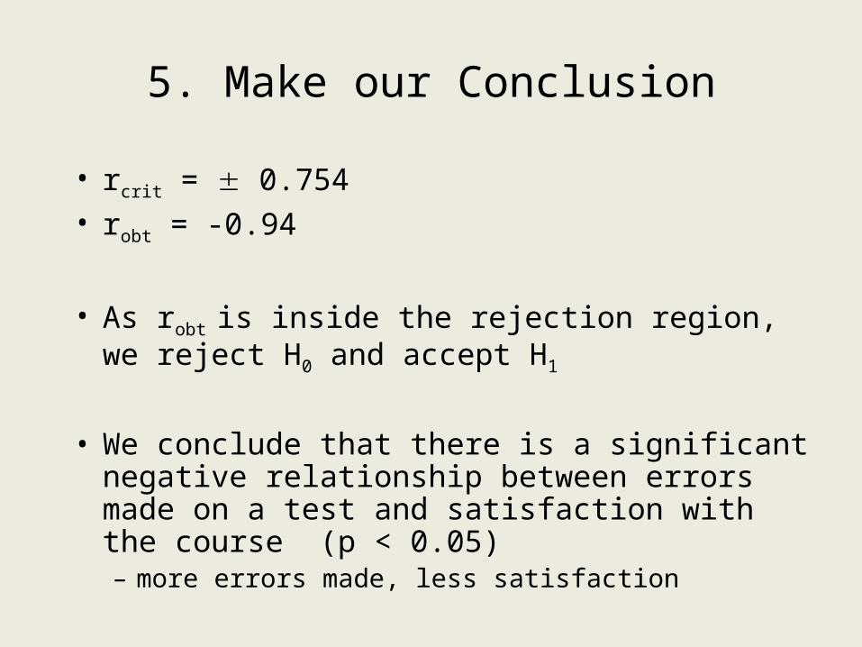
5. Make our Conclusion
• rcrit = 0.754• robt = -0.94
• As robt is inside the rejection region, we reject H0 and accept H1
• We conclude that there is a significant negative relationship between errors made on a test and satisfaction with the course (p < 0.05)– more errors made, less satisfaction
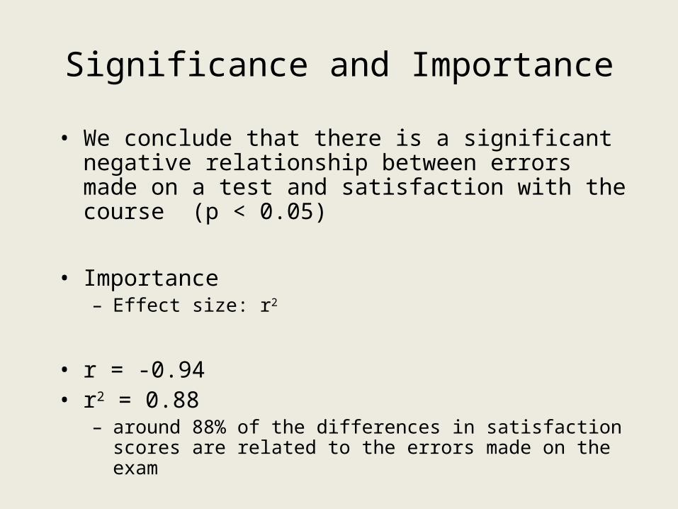
Significance and Importance
• We conclude that there is a significant negative relationship between errors made on a test and satisfaction with the course (p < 0.05)
• Importance – Effect size: r2
• r = -0.94• r2 = 0.88
– around 88% of the differences in satisfaction scores are related to the errors made on the exam
Homework
Chapter 8: 2, 6, 8