Saint Mary’s College of California

Department of Mathematics

Senior Thesis

Pseudorandom NumberGeneration

Author:

Matthew Dami

Committee:

Dr. Andrew Conner

Dr. Hans de Moor

May 16, 2016

1 Introduction

Random number generation is the process of creating long uniform se-

quences of numbers where it is impossible to predict the next number in the

sequence. There are two methods of generating random number sequences.

The first method is True Random Number Generation which measures events

in nature then a computer translates those events into a random sequence

of numbers. A common way to do this is by measuring the radioactive

decay from elements. The second method is Pseudorandom Number Genera-

tion which uses an algorithms to produce sequences of numbers that possess

random-like qualities.

Pseudorandom number sequences are most commonly used in Monte

Carlo simulations and other more general numerical simulations. These se-

quences are also heavily used in areas such as gambling and computer games.

In this paper we will concern ourselves with one common method used

to generate such sequences while using the following definition for random

number sequences. A sequence of numbers can be considered random

if it meets both of the following criteria: the values are uniformly distributed

over a defined interval or set, and it is impossible to predict future values

based on past or present ones. While we don’t have a strict mathematical

definition for randomness we can test both of these criteria mathematically.

2 Linear Congruential Method

The linear congruential method, and its variations, are the most commonly

used pseudorandom number generators. The linear congruential method can

1

be easily implemented using a computer and can quickly generate sequences.

The linear congruential generator produces a sequence, {Xn}, defined by

the following equation where a, c, m, X0 are all real numbers and chosen in

advance

Xn+1 ≡ (aXn + c) mod m, n ≥ 0

We choose the four integers; m, a, c, and X0 such that the following con-

ditions are met:

Table 1: Choosing the constants

m the modulus 0 < m

X0 the starting value 0 ≤ X0 < m

a the multiplier 0 < a < m

c the increment 0 ≤ c < m

The sequence created by the linear congruential generator is called a

linear congruential sequence. While any combination of integers will

produce a sequence, that sequence may not be pseudorandom. In this paper

we will discuss the primary method of picking integers that will produce a

pseudorandom sequence.

For an example let us consider the sequence when X0 = a = c = 7,

m = 10.

X1 = a ∗X0 + c mod m = 7 ∗ 7 + 7 mod 10 = 6

X2 = a ∗X1 + c mod m = 7 ∗ 6 + 7 mod 10 = 9

2

We continue this process to generate the sequence listed below:

7, 6, 9, 0, 7, 6, 9, 0, ...

These constants generate a sequence that illustrates two important issues

with the Linear Congruential Method. First, we are not guaranteed to get

a pseudorandom sequence for every choice of a, c, and m. Second, we will

always have a repeating cycle of numbers. The period is the length of the

shortest cycle of repeating numbers in a congruential sequence. So we would

say that the sequence when X0 = a = c = 7 and m = 10 has period of four.

When we have a short period it becomes easy to predict what values come

next.

Since we use modular arithmetic, (mod m) to generate a linear congru-

ential sequence, {Xn} we can have at most m different terms since each

Xn ∈ Zm where Zm = {0, 1, 2, ...,m− 1}. In the event that {Xn} has period

m, we say that the sequence has a maximum period. A primary issue we will

cover is how to choose our parameters to guarantee that our sequence will

have maximum period.

We can immediately dismiss a few impractical values of a. If a = 1, then

the resulting sequence would be generated by the equation Xn+1 ≡ (Xn + c)

mod m, which would produce a sequence where each value increases by c

making it very easy to predict what values will come next. The worst case

situation would be a = 0, which would always produce a sequence with period

two. Thus, we will assume that a ≥ 2.

The letters a, c, m, and X0 are used throughout this paper in the same

manner as stated in Table 1. It is also useful to define b = a − 1 and to

let Z+ denote all positive integers greater than 0, as they will be used in

3

many equations and theorems. Following the logic from above we can say

for practical reasons b ≥ 1.

We will now prove an alternative non-recursive formulation of the linear

congruential sequence which provides a tool for finding the nth term of a

sequence based on only a, c, m, and X0.

Lemma 2.1. Let {Xn} be a linear congruential sequence. Assuming that

a ≥ 2 then

Xn+k = (akXn + (ak − 1)c/b) mod m, k ≥ 0, n ≥ 0.

Proof. The proof is by induction on k. For the base case of k = 0 we can

clearly see that the lemma is true since Xn+0 = a0Xn + (a0 − 1)c/(a − 1)

mod m. Assume the lemma is true for the (n+ k)th term of {Xn}, and now

consider the (n+ k + 1)st term.

Xn+(k+1) = aXn+k + c (mod) m, by the LCS

= a

(akXn +

(ak − 1)c

(a− 1)

)+ c (mod) m, by induction assumption

= ak+1Xn +a(ak − 1)c

(a− 1)+ c (mod) m

= ak+1Xn +

(a(ak − 1)

(a− 1)+ 1

)c (mod) m

= ak+1Xn +(ak+1 − 1)c

(a− 1)(mod) m

We now have the required equation for the (n + k + 1)st term of {Xn}.

Therefore, by mathematical induction, the lemma is true for all k ≥ 0.

4

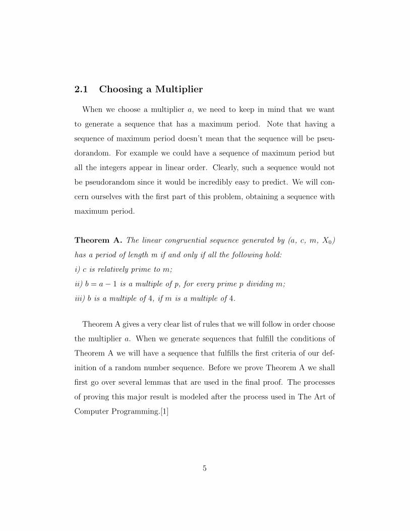
2.1 Choosing a Multiplier

When we choose a multiplier a, we need to keep in mind that we want

to generate a sequence that has a maximum period. Note that having a

sequence of maximum period doesn’t mean that the sequence will be pseu-

dorandom. For example we could have a sequence of maximum period but

all the integers appear in linear order. Clearly, such a sequence would not

be pseudorandom since it would be incredibly easy to predict. We will con-

cern ourselves with the first part of this problem, obtaining a sequence with

maximum period.

Theorem A. The linear congruential sequence generated by (a, c, m, X0)

has a period of length m if and only if all the following hold:

i) c is relatively prime to m;

ii) b = a− 1 is a multiple of p, for every prime p dividing m;

iii) b is a multiple of 4, if m is a multiple of 4.

Theorem A gives a very clear list of rules that we will follow in order choose

the multiplier a. When we generate sequences that fulfill the conditions of

Theorem A we will have a sequence that fulfills the first criteria of our def-

inition of a random number sequence. Before we prove Theorem A we shall

first go over several lemmas that are used in the final proof. The processes

of proving this major result is modeled after the process used in The Art of

Computer Programming.[1]

5

Lemma 2.2. Let p be a prime number, and let e ∈ Z+, where pe > 2. If

X ≡ 1(modulo pe) and X 6≡ 1(modulo pe+1) (A)

then

Xp ≡ 1(modulo pe+1) and Xp 6≡ 1(modulo pe+2). (B)

Proof. Assume statement (A) is true, then X = 1 + qpe for some q ∈ Z and

not a multiple of p. By the binomial theorem

Xp =(1 + qpe)p

=1 +

(p

1

)qpe + ...+

(p

p− 1

)qp−1p(p−1)e + qpppe

=1 + qpe+1

(1 +

1

p

(p

2

)qpe +

1

p

(p

3

)q2p2e...+

1

p

(p

p

)qp−1p(p−1)e

)Since e ≥ 1, the quantity contained in the parentheses (q′) is an integer.

If 1 < k < p then(pk

)is divisible by p. Therefore 1

p

(pk

)qk−1p(k−1)e is divisible

by p(k−1)e. The last term 1p

(pp

)qp−1p(p−1)e = qp−1p(p−1)e−1 is divisible by p,

because (p − 1)e > 1 when pe > 2. Thus every term, except for the first, is

divisible by p. Therefore, Xp = 1 + q′pe+1, where q′ ∈ Z and not divisible by

p, this implies that Xp ≡ 1(modulo pe+1) and Xp 6≡ 1(modulo pe+2).

Lemma 2.3. Let m = pe11 pe22 ...p

ehh be the decomposition of a positive integer

m into distinct prime factors. The length, α, of the period of the linear

congruential sequence {Xf} determined by (X0, a, c, m) is the least common

multiple of lengths αg of the periods of the linear congruential sequences (X0

mod pegg , a mod p

egg , c mod p

egg , p

egg ), 1 ≤ g ≤ h.

Proof. By mathematical induction on h, it is only necessary to prove that if

i and u are relatively prime where GCD(i, u) = 1, then the period length, α,

6

of the given sequence {Xf} is the least common multiple of the lengths α1,

α2 of the respective period lengths of the sequences respectively {Yf} and

{Zf} given by (X0 mod i, a mod i, c mod i, i) and (X0 mod u, a mod u, c

mod u, u).

We then have by definition of the three sequences have Yf ≡ Xf (mod i)

and Zf ≡ Xf (mod u) for all f ≥ 0. Because (i, u) = 1, then

Xf = Xg if and only if Yf = Yg and Zf = Zg. (C)

Let α′ be the least common multiple of α1 and α2. Since the sequence

{Yf} has period α1, we can say Yf = Y0 if and only if f is is a multiple of α1.

By the same logic the sequence {Zf} has period α2, we can say Zf = Z0 if

and only if f is is a multiple of α2. Notice that f must be a multiple of both

α1 and α2. We will prove this with the argument below.

By definition, {Zf} has period α so Xα ≡ X0 mod m and Xn 6≡ X0 for

all 0 < n < α. Since Xα ≡ X0 mod m then m divides Xα − xx0 . Because i

divides m, then i also divides Xα − X0. Therefore Xα ≡ X0 mod i and by

extension Yα ≡ Y0 mod i. Let α1 be the period of {Yf}; and the argument

above, α1 ≤ α.

By the Division Algorithm α = qα1 + r for q ∈ Z, 0 ≤ r < α1. Also by

lemma 2.1;

Y0 ≡ Yα = Yqα1+r = aqα1Yr +(aqα1 − 1)c

bmod i

but aα1 ≡ 1 mod i. To prove this, we want to show that Yq′α1 ≡ Y0 mod i

for any q′ ≥ 1. We know that Yα1 ≡ Y0 is equivalent to aα1 ≡ 1 mod i by

7

lemma 2.1. We can prove this by using induction on lemma 2.1:

Yq′α1 = aα1Y(q′−1)α1 +(aqα1 − 1)c

bmod i

= 1Y(q′−1)α1 + 0 mod i

= Y0 mod i by induction hypothesis

Thus Y0 ≡ Yr mod i and recall with the Division Algorithm we stated

that 0 ≤ r < α1. By definition of period, we can’t have 0 < r < α, so r = 0.

Therefore, α = qα1.

We now wish to prove that α′ = α. Since Xf = Xf+α for large values

of f , we have Yf = Yf+α (therefore α is a multiple of α1) and Zf = Zf+α

(therefore α is a multiple of α2), so α must be ≥ α′. Moreover, we also

know that Yf = Yf+α′ and Zf = Zf+α′ for all large values of f ; by equation

(C) above, Xf = Xf+α′ by a similar argument as above we find α|α′. Thus

α = α′.

Lemma 2.4. If a ≡ 3 (mod 4), then (a2e−1 − 1)/(a− 1) ≡ 0 (mod 2e), while

e > 1.

Proof. Suppose that a ≡ 3 (mod 4), then we can say that a = 3 + 4l when

l ∈ Z. This is equivalent to a = 1 + (2 + 4l) and also a = 1 + 2(1 + 2l). This

then implies that a ≡ 1 (mod 2).

We now have a2 = 9 + 24l+ 16l2 = 1 + 8(1 + 3l+ 2l2). Thus a2 ≡ 1 (mod

8). By continued application we find that a4 ≡ 1 (mod 16), a8 ≡ 1 (mod 32),

and so on. Let us show this by use of induction:

8

a2n ≡ 1 mod 2n+2 Induction hypothesis

a2n

= 1 + 2n+2k Change form of equation

a2n+1

= (1 + 2n+2k)2 Begin induction

= 1 + 2n+3k + 2n+4k2

= 1 + 2n+3(k + 2n+1k2)

a2n+1

= 1 mod 2n+3 Desired out come

Therefore a2e−1−1 ≡ 0 (mod g2e+1). So a2

e−1−1 = 2e+1 for some g ∈ Z+.

Therefore (a2e−1−1)/2 = g2e, thus (a2

e−1−1)/2 = 0 (mod 2e) and this yields

the desired result.

We now have the tools required to begin proving Theorem A. Due to

Lemma 2.3 it is sufficient to prove Theorem A if we can prove that m is

a power of a prime number. If {Xn mod peii } has maximal period for all i

then {Xn} has maximal period. Let pe11 ...pehh = lcm(α1, ..., αh) ≤ α1...αh ≤

pe11 ...pehh be true if and only if αg = p

egg for 1 ≤ g ≤ h.

We can then assume that m = pe when p is prime and e ∈ Z+. Because

of our restrictions upon a it suffices to look at a > 1. Since the sequence is

periodic there is no loss of generality in claiming that X0 = 0

By Lemma 2.1

Xf =(af−1a−1

)c mod m.

If c is not relatively prime to m, then Xf can never be equal to 1. So condition

(1) from theorem A is required. The sequence has maximal period if and only

9

if the smallest positive value of f for which Xf = X0 = 0 is n = m. Using

lemma 2.1 and condition (1), it is sufficient to prove the following lemma.

Lemma 2.5. Assume that 1 < a < pe, where p is prime and 3 > 1. If α is

the smallest positive integer for which (aα−1)/(a−1) ≡ 0 (modulo pe), then

α = pe if and only if a ≡ 1 (mod p) when p > 2, and a ≡ 1 (mod 4) when

p = 2.

Proof. Assume that α = pe.

(af − 1)/(a− 1) ≡ 0 mod pe

implies that

ape ≡ 1 mod pe

hence

ape ≡ 1 mod p

If α 6≡ 1 (mod p), then (af − 1)/(a − 1) ≡ 0 (mod pe) if and only if

af − 1 ≡ 0 (mod pe). The condition ape − 1 ≡ 0 (mod pe) then implies that

ape ≡ 1 (mod p); but ap

e ≡ a (mod p); hence a 6≡ 1 (mod p) leads to a

contradiction.

If p = 2 and a ≡ 3 (mod 4), then (a2e−1 − 1)/(a − 1) ≡ 0 (mod 2e) by

Lemma 2.4. Thus α ≡ 1 mod 4 when p = 2, completing the first part of the

proof.

These arguments show that a ≡ 1 mod p, when p > 2 and additionally

a ≡ 1 mod 4, when p = 2 is equivalent to the statement that a = 1 + qpw

where pw > 2 and q is not a multiple of p.

It still needs to be shown that this condition is sufficient to make α = pe.

By Lemma 2.2, we see that for any positive integer c, apc ≡ 1 (mod pw+c),

10

and apc 6≡ 1 (mod pw+c+1). Therefore, (ap

c − 1)/(a − 1) ≡ 0 (mod pc) and

(apc − 1)/(a− 1) 6≡ 0 (mod pc+1), respectively.

In particular, (ape − 1)/(a − 1) ≡ 0 (mod pe). Now the congruential

sequence (0, a, 1, pe) has Xf = (af − 1)/(a− 1) (mod pe). Therefore it has

a period length of α and Xn = 0 if and only if n is a multiple of α. Then

pe is a multiple of α. This can only happen when α = pc for some c. While

(apc − 1)/(a− 1) ≡ 0 (mod pc) and (ap

c − 1)/(a− 1) 6≡ 0 (mod pc+1) implies

that α = pe. Thus completing the proof.

This also serves as the proof for Theorem A. Now let’s take a look at an

example.

Example: Let m = 63 and X0 = 0. To meet the conditions of our

theorem we first find the prime factors of m, which are 32 and 7.

Table 2: Candidates for the value of a

factors of b value of b value of a

3 ∗ 3 ∗ 7 63 64

2 ∗ 3 ∗ 7 42 43

3 ∗ 7 21 22

We can clearly see that a = 64 won’t work as it is greater than our value

for m. This leaves us with the values 43 and 22. These are the only values

of a that will produce a sequence with maximum period. It is important to

notice that b = 42 contains a prime factor, 2, which is not a prime factor

of 63. This is completely acceptable as long as 42 contains at least one of

every prime factor of m. This satisfies condition (2) of our theorem. To meet

11

condition (1) of the theorem we can simply set c equal to a prime number

that is not a prime factor of m.

3 Testing a Sequence

A common way to test a given sequence for pseudorandomness is with

a χ2 test, which takes a sample sub-sequence and compares the frequency

at which numbers appear with what would be expected in a true random

sequence. This method, has a major drawback; it requires the sequence to

already be generated and requires multiple tests of the sub-sequences. This

method tends to be time consuming when we deal with sequences that have

large periods. A better test to use on a Linear Congruential Sequence would

to test the sequence based solely on the parameters a, m, and c.

We can begin by examining the a priori test presented in Theorem B

and the corresponding proof. The idea of the theorem is that a truly random

sequence will have Xn+1 < Xn about half the time.

Theorem B. Let X0, a, c, and m generate a linear congruential sequence

with maximum period; let b = a− 1 and let d be the greatest common divisor

(GCD) of m and b. The probability that Xn+1 < Xn is equal to 12

+ r, where

r = (2(c mod d)− d)/2m;

hence |r| < d/2m.

It is important to note that this theorem only applies when we choose X0,

a, c, and m such that the sequence generated has the maximum period length

12

of m. Theorem A provides the tools necessary to choose our parameters so

that we can apply Theorem B.

To prove Theorem B we require several techniques, some of which are

interesting on their own. First we need to define a function s : Zm → Zm by

s(X) = (aX + c) mod m. (1)

Then we have, Xn+1 = s(Xn), and we can reduce the theorem to counting

the number of X ∈ Zm such that s(X) < X. We want to show that this

number is

12(m+ 2(c mod d)− d). (2)

When a = 1 we can see that s(X) < X only when X + c ≥ m, and that

there are c such cases.

For a real number x; the floor operation, bxc, is equal to the largest

integer less than or equal to x and the ceiling operation, dxe, is equal to the

smallest integer greater than or equal to x.

Lemma 3.1. Let α and β be real numbers and let n be an integer. Then

α < n < β if and only if bαc < n ≤ bβc; (3)

α < n < β if and only if dαe ≤ n < dβe. (4)

These formulas come directly from the definitions of the floor and ceiling

operations.

For any X such that 0 ≤ X < m, let k(X) = b(aX + c)/mc. Then

s(X) = aX + c− k(X)m and k(X) ≤ (aX + c)/m; therefore it follows that

s(X) < X is equivalent to

13

(k(X)m− c)/a ≤ X < (k(X)m− c)/b. (5)

With Lemma 3.1 and equation (5) we have the following inequalities.

Lemma 3.2. We find that s(X) < X and 0 ≤ X < m if and only if:

i) d(km− c)/ae ≤ X < d(km− c)/be for some k, 0 < k < a:

or

ii) dm− c/ae ≤ X < m.

Furthermore, the conditions i) and ii) are mutually exclusive.

Using these inequalities we are able to obtain the following the equation.

Lemma 3.3. The number of integers X such that s(X) < X is:

|{X|0 ≤ s(X) < X < m}| = m+∑

0<k≤b

d(km− c)/be−∑

0<k≤b

d(km− c)/ae. (7)

Theorem B will be proved if we can show that the equations (7) and (2)

are equal to each other. It will be helpful to introduce the following functions;

the latter of which is the ”sawtooth” function often used in the Fourier series.

We will now define the δ and ζ functions as they will be used in the following

proofs.

δ(z) = bzc+ 1− dze =

1, if z ∈ Z

0, if z 6∈ Z(8)

ζ(z) = z − bzc − 1

2+

1

2δ(z) = z − dze+

1

2− 1

2δ(z) (9)

The function ζ(z) has several useful properties:

ζ(−z) = −ζ(z) because b−zc = −dze; (10)

14

ζ(z + n) = ζ(z), if n ∈ Z; (11)

The third property requires a short proof to show how we arrive at it as

demonstrated in Lemma 3.4.

Lemma 3.4. If n ∈ Z+ then;

ζ(z) + ζ

(z +

1

n

)+ ...+ ζ

(z +

n− 1

n

)= ζ(nz) (12)

Proof. Let d = z − bzc be the decimal part of z. fix n ∈ Z. There exists

k ∈ Z such thatk

n≤ d <

k + 1

n≡ 0 ≤ nd− k < 1.

Then ζ(nz) = nd− k − 12

= nd− 2k+12. Also

δ

(z +

i

n

)=

d+ in− 1

2, for 0 ≤ i ≤ n− 1− k

d+ in− 1− 1

2for n− k − 1 < i ≤ n− 1

Therefore

n−1∑i=0

ζ

(z +

i

n

)= nd+

n−1∑i=0

i

n− k − n

2

= nd+1

n∗ n(n− 1)

2− 2k + n

2

= nd− 2k + 1

2

Lemma 3.5. By changing the notation of equation (7) we can get:

1

2

(m− 1 +

∑0<k≤a

δ

(km− ca

)−∑

0<k≤b

δ

(km− c

b

))

+∑

0<k≤a

ζ

(km− ca

)−∑

0<k≤b

ζ

(km− c

b

). (13)

15

Proof. We first observe that:⌈km−cb

⌉= km−c

b− ζ

(km−cb

)+ 1

2− 1

2δ(km−cb

)and we find that the equation for

⌈km−ca

⌉is similar. We can apply these

observations to equation (7) to transform it into:

m+∑

0<k≤b

km− cb

−∑

0<k≤b

ζ

(km− c

b

)+b

2− 1

2

∑0<k≤b

δ

(km− c

b

)

−∑

0<k≤a

km− ca

−∑

0<k≤a

ζ

(km− ca

)− a

2+

1

2

∑0<k≤a

δ

(km− ca

)

= m+m

b∗ b(b+ 1)

2− c+

b

2− m

a∗ a(a+ 1)

2+ c− b

2

−∑

0<k≤b

ζ

(km− c

b

)−1

2

∑0<k≤b

δ

(km− c

b

)−∑

0<k≤a

ζ

(km− ca

)+

1

2

∑0<k≤a

δ

(km− ca

)For simplicity we will now omit the summations from the following simplifi-

cations, but they will be re-added in the final equation. Recall that b = a−1.

m+m(b+ 1)

2+b

2− m(a+ 1)

2− a

2

m+ma

2+a− 1

2− m(a− 1)

2− a

2

m− m

2− 1

2

We will now re-add the summations:

m

2− 1

2−∑

0<k≤b

ζ

(km− c

b

)− 1

2

∑0<k≤b

δ

(km− c

b

)

−∑

0<k≤a

ζ

(km− ca

)+

1

2

∑0<k≤a

δ

(km− ca

)Which we find is equal to equation (13):

=1

2

(m− 1 +

∑0<k≤a

δ

(km− ca

)−∑

0<k≤b

δ

(km− c

b

))

16

+∑

0<k≤a

ζ

(km− ca

)−∑

0<k≤b

ζ

(km− c

b

)Thus we have shown that by changing notation we can transform equation

(7) into equation (13).

While this equation may look more complicated than what we began

with, all of the sums that occur can be evaluated easily. This is due to the

fact that m is relatively prime to a and we know that (km− c) mod a takes

on each of the values 0, 1,..., a− 1 in some order since 0 < k ≤ a. Therefore:∑0<k≤a

δ

(km− ca

)= 1, and

∑0<k≤a

ζ

(km− ca

)= 0.

Let’s show that the second formula holds true.∑0<k≤a

ζ

(km− ca

)=∑

0<k≤a

ζ

((km− c) mod a

a

)by equations (10) and (11)

=∑

0<i≤a−1

ζ

(i

a

)by comments preceding the formula

=

(a−1∑i=0

i

a

)− (a− 1)

2

=1

a∗ a(a− 1)

2− (a− 1)

2

= 0

Since m is not relatively prime to b but c is, then (km− c)/b 6∈ Z for any k.

Therefore we can say that the second sum in equation (13) is equal to zero.

Finally we can see that for any 0 < k ≤ b

17

ζ

(km− c

b

)= ζ

(km− dbc/dc − c mod d

b

)= ζ

(km/d− bc/dc

b/d

)− c mod d

b+

1

2δ

(km/d− bc/dc

b/d

),

since 0 ≤ (c mod d)/b < 1(b/d). The sum∑0<k≤b

ζ

(km− c

b

)therefore becomes 1

2d− c mod d. This is because

ζ

(km− c

b

)= ζ

(km/d− bc/dc

b/d

)− c mod d

b+

1

2δ

(km/d− bc/dc

b/d

)and since m/d is relatively prime to b/d. This establishes Theorem B.

Trying to implement Theorem B and generate a LCS by hand can be a

time consuming process. It is more efficient to use a programming language

to test our choices for a, c, m, and X0. An example of a program in Python

can be found in Appendix A. This code computes the r value and can also

generate the sequence to test that the expected probability of Xn+1 < Xn is

equal to the actual results. This also allows the user to make sure that the

generated sequence has maximal period.

From Theorem B we can see that when we have a sequence of maximum

period, nearly any choice of a and c will give a good probability that Xn+1 <

Xn, except when we have a large d value.

4 Potency

For a LCS to be pseudorandom the value of a must produce a large amount

of mixing between random numbers. When we have several options for our

18

value of a we can examine each one to determine their potency.

Potency is a measurement of the mixing of numbers in a linear congru-

ential sequence. This measurement is the smallest positive integer s that

satisfies the equation:

(a− 1)s = bs = 0 (mod m)

We are guaranteed an integer s exists when the multiplier a meets all the

conditions of Theorem A. This is due to the fact that b is divisible by every

prime factor of m. Because potency is a measure of mixing, we want to pick

an a that has the largest s. The higher the potency, the better the mixing.

In general. we want a potency of at least four in order to obtain minimal

acceptable levels of mixing.[1]

There is an important connection between potency and Theorem B. In

Theorem B, We want the value of d to be as close to one as possible as it

will produce an r value that is closer to zero because |r| < d/2m. We have

high potency when d is small compared to m, but we know that when the

integer s is large we also have high potency. So if two potential values for

a have the same potency we can also test the d value to determine if one is

better than the other.

For an example consider m = 4862025 which has the prime factorization

{345274}. The table below shows some of the possible values of b and their

corresponding values for s. For simplicity we have chosen values of b that

will also be equal to its corresponding d value.

19

Table 3: Five Potential values for b and the corresponding potency

factors of b value of b bs = 0 (mod m)

3 ∗ 5 ∗ 7 105 1054 = 0 (mod 4862025)

3 ∗ 3 ∗ 3 ∗ 5 ∗ 7 945 9454 = 0 (mod 4862025)

3 ∗ 3 ∗ 5 ∗ 7 ∗ 7 2205 22052 = 0 (mod 4862025)

3 ∗ 3 ∗ 3 ∗ 5 ∗ 5 ∗ 7 4725 47254 = 0 (mod 4862025)

3 ∗ 3 ∗ 3 ∗ 5 ∗ 5 ∗ 7 ∗ 7 231525 2315252 = 0 (mod 4862025)

We can clearly see that options three and five are poor choices as they

have s values of 2. This leaves us with three options for our multiplier, but

due to Theorem B we can narrow it down further. By Theorem B, option

one should also produce an r value that is closer to .5 than the other options.

We compute the r values of options one, two, and four to be certain that our

intuition is correct. We will be setting the increment as c = 11.

When b = 105:

r =2(11 mod 105)− 105

2 ∗ 4862025= −8.53553817 ∗ 10−6

When b = 945:

r =2(11 mod 945)− 945

2 ∗ 4862025= −9.4919298 ∗ 10−5

When b = 4725:

r =2(11 mod 4725)− 4725

2 ∗ 4862025= −4.83646217 ∗ 10−4

This shows that option one is the best choice for our multiplier for when

m = 4862025. It satisfies the conditions listed out in theorem A, has a large

20

value for s, and has the closest d value that is close to zero. All of these

tools are needed in order to choose good parameters for generating a linear

congruential sequence. Theorem A gives us a way to produce a sequence

with maximal period so our sequences will be uniform, potency allows us

to measure if our sequences will be predicable, and with Theorem B we can

test our choices of a, c, and m to help us determine if our parameters were

well chosen. While Theorem A and potency allow us to test a and m, only

Theorem B gives us a method for determining if our choice for c is good.

21

References

[1] Knuth, D. E. (1998) The Art of Computer Programming Volume 2:

Semi-numerical Algorithms. Boston: Addison-Wesley, 1998. Print.

[2] ”Linear Congruential Generator.” Wikipedia. Wikimedia Foundation,

13 Mar. 2016. Web. 20 Apr. 2016.

[3] Nguyen, Hubert. (2008) GPU Gems 3. Upper Saddle River, NJ:

Addison-Wesley, 2008. GPU Gems. Web. 20 Apr. 2016.

[4] ”True Random Number Service.” RANDOM.ORG. N.p., n.d. Web. 20

Apr. 2016.

22

Appendix A

import math

import f r a c t i o n s

def main ( ) :

##Counts the amount o f t imes the sequence increased .

s h i f t up = 0

##Counts the amount o f t imes the sequence decreases .

sh i f tdown = 0

##The i n i t i a l number in the sequence .

##Since the sequence w i l l have a maximum period ,

##where we beg in our sequence i s t r i v i a l .

seed = int ( )

##The mu l t i p l i e r .

mult = input ( ”What i s the mu l t i p l i e r ? ” )

mult = int (mult )

#The increment .

i n c r e = input ( ”What i s the increment ? ” )

i n c r e = int ( i n c r e )

##The modulus .

mod = input ( ”What i s the modulus? ” )

mod = int (mod)

##I n i t i a l i z e s the l i s t t h a t w i l l ho ld the sequence .

##Places the seed in to the sequence .

h o l d i n g l i s t = [ seed ]

#Theore t i c a l t e s t s to determine i f sequence w i l l be psudorandom .

#Se t t i n g peramaters .

b = mult − 1

23

d = f r a c t i o n s . gcd (b , mod)

print ( ”The value o f d i s ” , d )

r = (2∗ ( i n c r e % d) − d )/(2∗mod)

##The wh i l e loop s t op s once a number has been repea ted .

while ( h o l d i n g l i s t . count ( seed ) !=2) :

xseed = seed

seed = ( ( ( mult∗ seed)+ in c r e )% mod)

h o l d i n g l i s t . append ( seed )

#The i f s ta tement checks to see i f the sequence

##has increased or decreased

i f xseed < seed :

s h i f t up += 1

else :

sh i f tdown += 1

#Removes the repea ted number .

k = h o l d i n g l i s t . pop ( )

## Zed i s the l e n g t h o f the per iod .

zed = len ( h o l d i n g l i s t )

print ( ”This sequence has a per iod o f ” , zed )

##The p r o b a b i l i t y t h a t X (n+1) < X n

prob = shi f tdown / zed

print ( r )

r += 0 .5

print ( ”The p r obab i l i t y that X (n+1) < X n = ” , r )

##Prin t s the generated sequence

## Causes problems wi th l onger sequences .

print ( h o l d i n g l i s t )

24