Embed Size (px)
Citation preview
Pseudo-observations in survival analysis
Master of Science Thesis
Autumn 2012/Spring 2013
Rikke Nørmark Mortensen
Department of Mathematical Sciences Aalborg University

Institut for Matematiske FagFredrik Bajers Vej 7G9220 Aalborg Østhttp://www.math.aau.dk
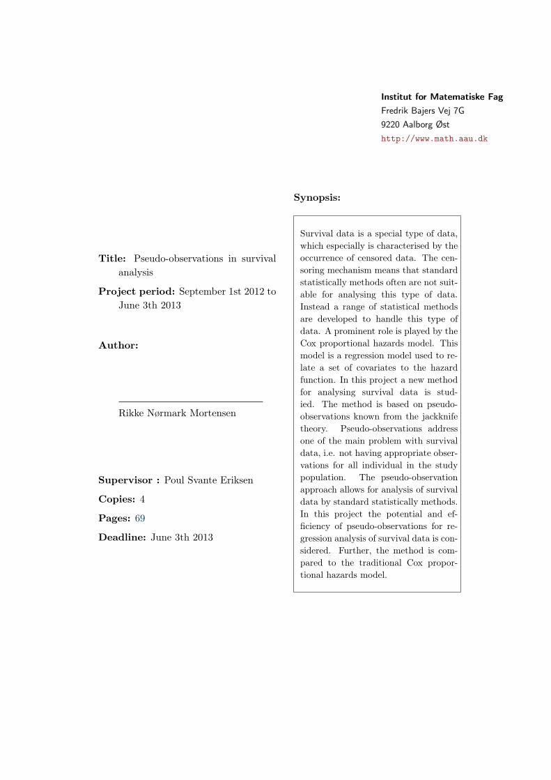
Title: Pseudo-observations in survivalanalysis
Project period: September 1st 2012 toJune 3th 2013
Author:
Rikke Nørmark Mortensen
Supervisor : Poul Svante Eriksen
Copies: 4
Pages: 69
Deadline: June 3th 2013
Synopsis:
Survival data is a special type of data,which especially is characterised by theoccurrence of censored data. The cen-soring mechanism means that standardstatistically methods often are not suit-able for analysing this type of data.Instead a range of statistical methodsare developed to handle this type ofdata. A prominent role is played by theCox proportional hazards model. Thismodel is a regression model used to re-late a set of covariates to the hazardfunction. In this project a new methodfor analysing survival data is stud-ied. The method is based on pseudo-observations known from the jackknifetheory. Pseudo-observations addressone of the main problem with survivaldata, i.e. not having appropriate obser-vations for all individual in the studypopulation. The pseudo-observationapproach allows for analysis of survivaldata by standard statistically methods.In this project the potential and ef-ficiency of pseudo-observations for re-gression analysis of survival data is con-sidered. Further, the method is com-pared to the traditional Cox propor-tional hazards model.

Dansk resume
Overlevelses data betegner en speciel type data som findes i mange empiriske studier, så somi epidemiologi, økonomiske studier og demografiske studier. Overlevelses data betegner entype data som måler tiden frem til en given hændelse. Variablen man er interesseret i ertiden frem til hændelses målt fra et givet begyndelses tidspunkt. Dette betyder at overlevelsesdata er opsamlet sekventielt, og dette har betydning for strukturen af dataet. Specielt vildenne opsamlings metode betyde at censureret hændelsestidspunkter kan forekomme for deleaf studiepopulationen. En censurering betyder at den faktiske hændelsestid ikke er kendt. Istedet har man observeret en censureringstid som enten er større eller mindre end den faktiskehændelsestid. Den mest almindelige censureringsmekanisme er højre censurering, hvilket vilsige at tidspunktet for hændelses er større end det observerede censureringstidspunkt. Struk-turen af overlevelses data betyder at traditionelle statistiske metoder ofte ikke kan anvendespå overlevelses data. Specielt er manglen på fuld information for dele af studiepopulationenet problem. En række statistiske modeller er udviklet specielt til at håndtere denne type data.En populær regressions model for overlevelses data er den proportionelle hazards Cox model.Dette er en semi-parametrisk regressionsmodel, brugt til at analysere effekten af en rækkekovariater på hazard funktionen.
I dette speciale er en ny metode til at analysere overlevelses data studeret. Denne metodebygger på pseudo-observationer kendt fra jackknife metoden. For hvert individ i studie popu-lationen er en mænge af pseudo-observation udregnet, hvilket giver et fuldstændigt data sæt.Dette fuldstændige data sæt giver mulighed for at analysere overlevelses data med standardstatistiske modeller, så som generaliseret lineær modeller. Dette giver mulighed for meregenerelle analyser af overlevelses data end standard overlevelses modeller tillader. I dettespeciale et regressions modeller baseret på pseudo-observationer sammenlignet med den tra-ditionelle Cox model.


Preface
This Master of Science thesis is written by Rikke Nørmark Mortensen in fall 2012 and spring2013 during the 9’th and 10’th semester of Mathematics at the Institute for MathematicalSciences at Aalborg University.
The reader of this thesis is assumed to possess the mathematical qualifications correspond-ing to completion of the bachelor education of Mathematical Sciences at Aalborg University.
I will like to thank Poul Svante Eriksen for supervision throughout the study period of thisproject.
Reading instructions
References throughout the report will be presented according to the Harvard method. Math-ematical definitions, figures, tables etc. are enumerated in reference to the chapter i.e. thefirst definition in chapter 2 has number 2.1, the second has number 2.2 etc. A reference toA.1 refer to the appendix.

Contents
1 Introduction 2
2 Basic quantities 4
2.1 Continuous random variables . . . . . . . . . . . . . . . . . . . . . . . . . . . . 4
2.2 Discrete random variables . . . . . . . . . . . . . . . . . . . . . . . . . . . . . . 9
3 Counting processes 10
3.1 The Nelson-Aalen estimator . . . . . . . . . . . . . . . . . . . . . . . . . . . . . 13
3.2 The Kaplan-Meier estimator . . . . . . . . . . . . . . . . . . . . . . . . . . . . . 15
4 Semiparametric proportional hazards models 16
4.1 The Cox proportional hazards model . . . . . . . . . . . . . . . . . . . . . . . . 174.1.1 The partial likelihood . . . . . . . . . . . . . . . . . . . . . . . . . . . . . 184.1.2 The partial likelihood for distinct event times . . . . . . . . . . . . . . . . . 194.1.3 The partial likelihood when ties are present . . . . . . . . . . . . . . . . . . 224.1.4 A discrete model analogue to the Cox proportional hazards model . . . . . . . 244.1.5 Estimation of the hazard function and the survival function . . . . . . . . . . 25
5 Pseudo-observations 28
5.1 Properties of the pseudo-observations . . . . . . . . . . . . . . . . . . . . . . . . 32
5.2 Regression models based on pseudo-observations . . . . . . . . . . . . . . . . . 36
5.3 Pseudo-residuals . . . . . . . . . . . . . . . . . . . . . . . . . . . . . . . . . . . 42
6 Regression splines 46
7 The new pseudo-observation 52
7.1 Properties of the new pseudo-observation . . . . . . . . . . . . . . . . . . . . . 54
7.2 Regression analysis based on the new pseudo-observation . . . . . . . . . . . . 56
1
1
8 Discussion and conclusion 62
9 Bibliography 66
A Appendix 68
A.1 The cumulative incidence function . . . . . . . . . . . . . . . . . . . . . . . . . 68
1Introduction
Survival data is a special type of data which arises in a number of applied settings such asmedicine, biology, epidemiology, economics, and demography. The term survival data is usedfor data which measures the time to some event of interest. In the simplest case the eventof interest is dead; however, the event of interest may also cover events like the onset ofsome disease or other complications. In this project, the terms event, dead, and failure willsynonymously be used as the occurrence of some event of interest.
Survival data possess a number of features which makes it differ from other types of data.The main different lies in the way the survival data is measured. In other types of data, theresponses are measured instantaneously and independent of the size of the response variable.In survival data the response variable is the event time, which is measured sequentially fromthe beginning of the study. This means that for survival data the large responses take longertime to measure than smaller responses. This way of measuring has a number of consequences,which must be dealt with when the survival data is analysed.
One consequence of the way survival data is measured is the occurring of censored data.The event time is said to be censored if the time of the event is not observed directly, but allthat is known is that the event occurred either before or after some observed time, called thecensoring time. The most common censoring mechanism is right censoring, which means thatthe event occurs at some time point after the observed censoring time. In some situations, rightcensoring occurs if an individual simply has not experienced the event before the terminationtime of the study. In other situations right censoring occurs if an individual leave the studybefore it is completed. If this early exit from the study is due to reasons unrelated to theevent of interest, the right censoring is said to be independt of the event time. Less commoncensoring mechanisms include left censoring and interval censoring. An individual is said tobe left censored if the event time is known to occur prior to the observed censoring time.Interval censoring means that the event is known to occur at some time within an interval.In this project, the term censored data will almost always refere to right censoring. Though,som eof the methods might be generalised to left censoring of interval censoring.
2
1. Introduction 3
Due to the structure of survival data, statistically models for analysing this type of datahave been developed as an independent area within statistics. Broadly the methods foranalysing survival data can be divided into non-parametric methods, parametric methods,and semi-parametric methods. Non-parametric methods serve to draw inference about theevent time distribution based on observed, possible censored data. Non-parametric methodsinclude the Kaplan-Meier estimator and the Nelson-Aalen estimator introduced in chapter3. These methods may be of interest on their own right or they may serve as a precursor tomore detailed analysis. Often the observed data contain some additional information abouteach individual, which can be used as covariates in a regression analysis. Parametric methodsmay be used for maximum likelihood estimation of the unknown parameters in the regressionmodel. However, from a practical point of view, the main objective when modelling survivaldata is to assess the effect of the covariates on the outcome of the regression model. Thisoutcome is often given as a function well suited to describe the information in survival data,these functions are discussed in chapter 2. The event time distribution is often of secondaryinterest. This means that specifying a full parametric model may be a too strict assumption forthe purpose of the analysis. More efficient results can often be obtained by a semi-parametricmodel. A semi-parametric model is a model in which the effect of the covariates is assumedto be parametric, but the effect of the time variable is given by some unspecified function.
A broad range of semi-parametric models have been developed for the purpose of analysingsurvival data. One of the most popular models is the Cox proportional hazards model. Thismodel is a flexible model which is well suited in many applied settings. Inference on this modelis based on a partial likelihood approach, in which the problem with censored data is handleby putting most emphasis on the observed event times.
In spite of the variety of models for analysis survival data, the occurrence of censored dataput a restriction on the possibilities within analysis for this type of data. One example is graph-ical methods, such as residual plots, which is inconvenient due to censored event times. If nocensoring occurs in the data, standard statistically models could be used to analyse the data.Standard statistically models often allows for more general analysis than the methods of sur-vival data. In this project, jackknife pseudo-observations are considered as a tool for analysingsurvival data. Pseudo-observations address one of the main problems with survival data, i.e.not having appropriate responses for all individuals in the study. Hence, this approach is astep in the direction of analysing censored survival data by standard statistically methods.The approach were first suggested by Andersen et al. [2003] for performing generalised linearregression analysis of survival data. The method is based on a set of pseudo-observationsdefined for each individual in the study. The pseudo-observation approach is a must generalmethod which may be applied in a number of applications. The aim of this project is toillustrate the potential and efficiency of this approach for regression analysis. Further, thepotential of the methods for topics related to the Cox proportional hazards model is likewiseconsidered.
2Basic quantities
This chapter is written based on Klein and Moeschberger [1997] and Hosmer and Lemeshow[1999].
In this chapter some basic quantities used to describe the distribution of survival data isconsidered. Let X be a nonnegative random variable denoting the time to some event. Thedistribution of X can be described by the cumulative distribution function F (t) = P(X ≤ t)
and when X is a continuous random variable, also by the density function f(t) = ddtF (t).
However, other functions are better suited to describe the distribution of time-to-event data.For survival data, one is often interested in the probability of surviving beyond the time t,this probability is given by the survival function. The hazard function describes the risk of anevent in the next instant, given that the event has not occurred prior to the time t. These fourfunctions all characterise different features of the distribution of X and given one of them, onecan uniquely determine the others. Other parameters of interest for describing survival dataare the mean survival time and the related restricted mean survival time, these two parametersare intuitive appealing in applied settings.
2.1 Continuous random variables
In this section, the basic functions for describing the survival distribution of non-negativecontinuous random variable X are given.
The survival function
The survival function is the most basic quantity to describe survival data. It gives the prob-ability of observing an event beyond the time t.
4
2. Basic quantities 5
Definition 2.1 The survival function of a non-negative random variable X is given by:
S(t) = P(X > t), t ≥ 0.
The survival function is related to the cumulative distribution function and the densityfunction in the following way
S(t) = 1− F (t)
=
∫ ∞t
f(u)du. (2.1)
The density function can hence be written in terms of the survival function as
f(t) = − d
dtS(t).
Equation (2.1) implies that
S(0) =
∫ ∞0
f(u)du = 1, (2.2)
and further
S(∞) = limy→∞
S(y)
= limy→∞
∫ ∞y
f(u)du
= 0. (2.3)
From (2.2) and (2.3) it is seen that the survival function is a decreasing function taken values inthe range of zero to one. Furthermore, equation (2.3) implies that an individual eventually isexpected to experience the event if this just live long enough. In many contexts where survivaldata appear this assumption is reasonable, for instance if the event of interest is dead, whichwill occur for everybody in time. However, in some settings it is unlikely that all individual inthe study eventually will experience the event, for instant if the event of interest is the timeof start smoking, which may or may not occur to everybody.
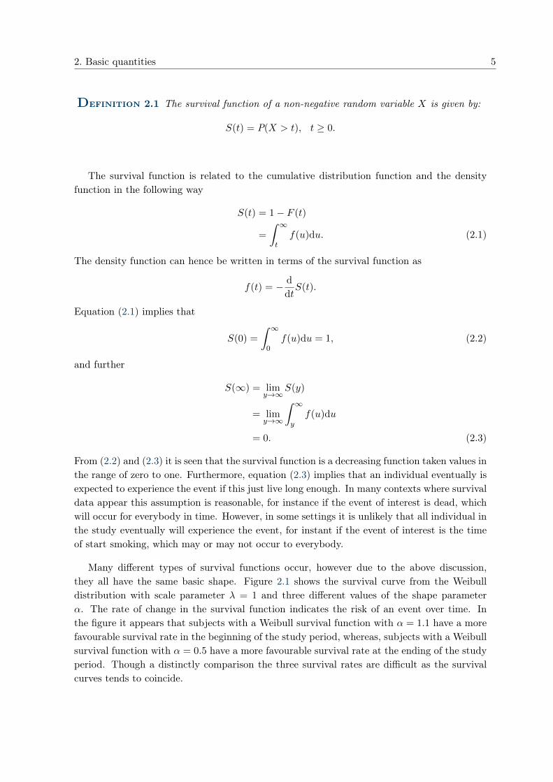
Many different types of survival functions occur, however due to the above discussion,they all have the same basic shape. Figure 2.1 shows the survival curve from the Weibulldistribution with scale parameter λ = 1 and three different values of the shape parameterα. The rate of change in the survival function indicates the risk of an event over time. Inthe figure it appears that subjects with a Weibull survival function with α = 1.1 have a morefavourable survival rate in the beginning of the study period, whereas, subjects with a Weibullsurvival function with α = 0.5 have a more favourable survival rate at the ending of the studyperiod. Though a distinctly comparison the three survival rates are difficult as the survivalcurves tends to coincide.
6 2.1. Continuous random variables
0.0 0.5 1.0 1.5 2.0 2.5
0.0
0.2
0.4
0.6
0.8
1.0
Time
Sur
viva
l fun
ctio
n
α = 1α = 0.5α = 1.1
Figure 2.1: The Weibull survival functions with three different values of the shape parameter α.
The survival function gives the initial probability of an individual to survive from the timeorigin to a time point beyond the time t. Hence, the changes in the risk of an event with timeare not captured in the survival function; another function which more properly describes thisis the hazard function.
The hazard function
The hazard function describes the instantaneous risk of an event at time t, given that the eventhas not occurred prior to time t. That is, the hazard function gives conditional informationon how the risk of an event changes with time.
Definition 2.2 The hazard function for a random variable X is defined as
h(t) = lim∆t→0
P(t ≤ X < t+ ∆t|X ≥ t)∆t
By the definition of h(·), the quantity h(t)∆t may be considered as an approximate con-ditional probability of an event in the interval [t, t+ ∆t). However, the hazard function itselfis not a probability, but may rather be considered as the rate for which the risk of an eventchanges with time. The values of the hazard function can vary between zero and infinity, andthe shape of h(·) can possess many different forms, reflecting the changes in the risk of anevent with time.
2. Basic quantities 7
0.0 0.5 1.0 1.5 2.0 2.5
0.0
0.5
1.0
1.5
Time
Haz
ard
func
tion
α = 1α = 0.5α = 1.1
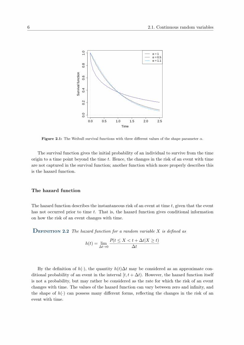
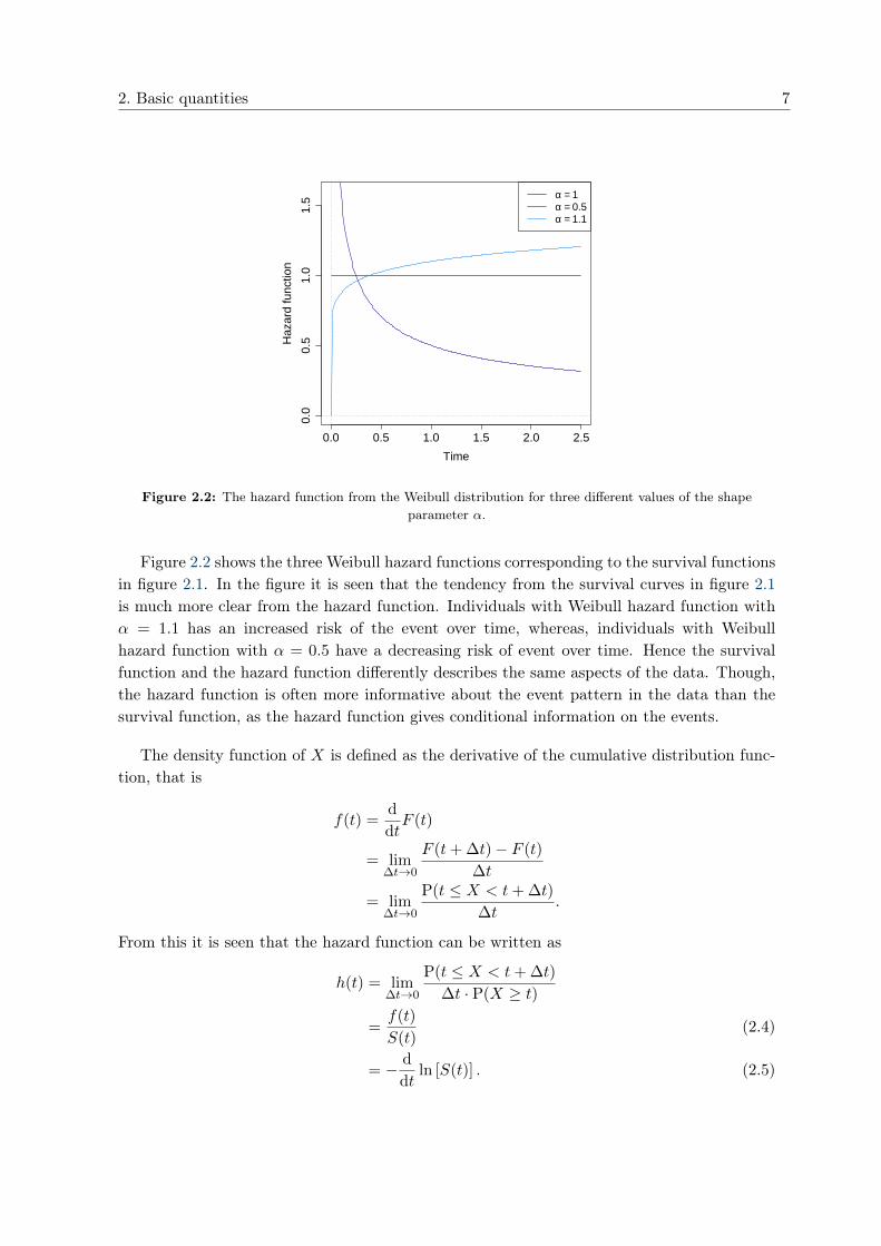
Figure 2.2: The hazard function from the Weibull distribution for three different values of the shapeparameter α.
Figure 2.2 shows the three Weibull hazard functions corresponding to the survival functionsin figure 2.1. In the figure it is seen that the tendency from the survival curves in figure 2.1is much more clear from the hazard function. Individuals with Weibull hazard function withα = 1.1 has an increased risk of the event over time, whereas, individuals with Weibullhazard function with α = 0.5 have a decreasing risk of event over time. Hence the survivalfunction and the hazard function differently describes the same aspects of the data. Though,the hazard function is often more informative about the event pattern in the data than thesurvival function, as the hazard function gives conditional information on the events.
The density function of X is defined as the derivative of the cumulative distribution func-tion, that is
f(t) =d
dtF (t)
= lim∆t→0
F (t+ ∆t)− F (t)
∆t
= lim∆t→0
P(t ≤ X < t+ ∆t)
∆t.
From this it is seen that the hazard function can be written as
h(t) = lim∆t→0
P(t ≤ X < t+ ∆t)
∆t · P(X ≥ t)
=f(t)
S(t)(2.4)
= − d
dtln [S(t)] . (2.5)
8 2.1. Continuous random variables
A function related to the hazard function is the cumulative hazard function.
Definition 2.3 Let X be a random variable with hazard function h(·), the cumulativehazard function of X is defined by
H(t) =
∫ t
0h(u)du.
From a practical point of view, the hazard function h(·) is often of main interest, as thisfunction is more intuitive clear. However, the cumulative hazard function H(·) is often easierto estimate from a given data set.
By equation (2.5) and the fundamental theorem of calculus, the cumulative hazard functionand the survival function is related in the following way
H(t) = − ln [S(t)] , (2.6)
and hence
S(t) = exp [−H(t)] (2.7)
= exp
[−∫ t
0h(u)du
]. (2.8)
Combining equation (2.4) with equation (2.8) one gets that the density function can be writtenin terms of the hazard function as
f(t) = h(t) exp
[−∫ t
0h(u)du
]. (2.9)
The mean survival time
Another parameter of interest is the mean survival time µ = E[X], which may be written as
µ =
∫ ∞0
S(t)dt,
where S(·) is the survival function of X. This parameter is intuitive appealing as it gives theexpected lifetime for an individual with survival function S(·).
When analysing survival data right censoring often occur. This means that the tail of thesurvival time distribution may be difficult to estimate and hence an estimate of µ may beheavily biased. A parameter related to the mean survival time is the restricted mean survivaltime.
2. Basic quantities 9
Definition 2.4 The restricted mean survival time for a random variable X is defined by
µτ = E[min(X, τ)],
for τ > 0.
This parameter gives the expected lifetime over the interval [0, τ ]. In similarity with themean survival time, the restricted mean may be written as
µτ =
∫ τ
0S(t)dt.
The restricted mean survival time is less sensitive to the occurrence of right censoring in agiven sample than the overall mean µ.
2.2 Discrete random variables
In this section, the discrete analogue to the functions described in the previous section is given.Let X be a discrete random variables taking values t0 < t1 < t2 < · · · and let p(·) denote theprobability function
p(ti) = P(X = ti), i = 0, 1, 2, . . .
The discrete survival function is then given by
S(t) =∑ti>t
p(ti). (2.10)
The hazard function at time ti is given by the conditional probability of failing at time ti,given survival until time ti, that is
h(ti) = P(X = ti|X ≥ ti) =p(ti)
S(ti−1),
whith the convenience that S(t0) = 1. Note that p(ti) = S(ti−1)− S(ti) from which it followsthat
h(ti) = 1− S(ti)
S(ti−1).
The discrete survival function (2.10) may be written as a product of conditional survivalfunctions
S(t) =∏ti≤t
S(ti)
S(ti−1),
and it follows that the survival function may be written in terms of the hazard function
S(t) =∏ti≤t
[1− h(ti)] .
3Counting processes
This chapter is written based on Fleming and Harrington [1991], Andersen et al. [1993], andKlein and Moeschberger [1997].
Survival data consist of observations gathered over a period of time, and it is natural tomodel this type of data as a stochastic process. Counting process methods provide exact waysfor studying incomplete data. In this chapter an introduction to counting process theory isgiven. The main object of this chapter is to define non-parametric estimators of the cumulativehazard function and the survival function.
Definition 3.1 A stochastic process N(t), t ≥ 0 is called a counting process if it fulfilsthe following properties: N(0) = 0; N(t) < ∞ a.s. and the sample paths of N(t) are withprobability one right-continuous and piecewise constant with jump of size +1.
Suppose a right censored sample with n individuals is given. Let Tj = min(Xj , Cj) bethe study time for individual j = 1, . . . , n and let δj = 1[Xj ≤ Cj ]. Here the event time Xj
and the censoring time Cj are assumed to be independent, continuous random variables. Theprocess Nj(t) = 1[Tj ≤ t, δj = 1] is then a counting process defined for each individual j.Summing over Nj(t) one gets a counting process
N(t) =
n∑j=1
Nj(t), (3.1)
which counts the number of events occurring prior to and including the time t.
The focus in this chapter is restricted to counting processes defined for right censoredsamples, though the theory may be applied in a more general setting. For a given rightcensored sample, the sample paths of the counting process N(·) given in (3.1) describes thetimes of events. Further, the difference N(t) − N(s) is the number of events in the interval
10
3. Counting processes 11
(s, t]. However, at a given time t additional information on the sample may available, suchas knowledge on censoring prior to t. The history of a counting process at time t is theaccumulated knowledge of the sample prior to and including the time t, and is denoted Ft.The history is assumed to be increasing, that is Fs ⊆ Ft, for all s < t.
Let N(·) be a given counting process and let t− denote the time just prior to but notincluding the time t, then the quantity dN(t) is defined as
dN(t) = N([t+ dt]−
)−N
(t−)
dt > 0.
That is, dN(·) is the change in the counting process over the interval [t, t + dt). If dt issufficiently small then the quantity dN(t) is a zero-one random variable, meaning that eitheran event occur in the interval [t, t+ dt) or no event occur in the interval.
Definition 3.2 The intensity process λ(·) of a counting process N(·) is defined as
λ(t) = limdt→0
P (dN(t) = 1|Ft−)
dt.
For a right censored sample, the probability of individual j failing in a small interval[t, t+ dt) is given by
P (t ≤ Tj < t+ dt, δj = 1|Ft−) , j = 1, . . . , n. (3.2)
For Tj < t the probability in (3.2) is obviously equal zero. For Tj ≥ t, the probability is givenby
P (t ≤ Tj < t+ dt, δj = 1|Ft−) = P (t ≤ Xj < t+ dt, Cj ≥ t+ dt|Xj ≥ t, Cj ≥ t)= P (t ≤ Xj < t+ dt|Xj ≥ t) · P (Cj ≥ t+ dt|Cj ≥ t)
=[F (t+ dt)− F (t)]
S(t)· P (Cj ≥ t+ dt|Cj ≥ t)
=f(t)dt
S(t)· P (Cj ≥ t+ dt|Cj ≥ t)
≈ h(t)dt,
for dt sufficiently small. Her h(·) is the hazard function given in definition 2.2
Let Y (t) be the risk set at time t, that is Y (·) is process describing the number of individualsat risk at some given time;
Y (t) =
n∑j=1
1[Tj ≥ t].
12
Then for dt sufficiently small
P (dN(t) = 1|Ft−) = E [dN(t)|Ft− ]
= E[#{j : Tj ∈ [t, t+ dt), δj = 1}
∣∣Ft− ]= Y (t)h(t)dt,
where N(·) is the counting process in (3.1). Hence, for a right censored sample the intensityfunction is given by λ(t) = Y (t)h(t).
Definition 3.3 Let N(·) be a counting process with intensity function λ(·), the cumulativeintensity process is then defined by
Λ(t) =
∫ t
0λ(u)du, t ≥ 0.
The general theory of martingales is a concept which arises naturally in the context ofcounting processes. A martingale is a stochastic process with the property that the expectedvalue of the next observation from the process given the history is equal to the present obser-vation. A stochastic process M(·) is called a martingale if it fulfils
E[M(t)|Fs] = M(s), for all s ≤ t. (3.3)
Definition 3.4 Let N(·) be a counting process with cumulative intensity function Λ(·),then the counting process martingale is defined as
M(t) = N(t)− Λ(t).
The counting process martingale has the property that
E[dM(t)|Ft− ] = E[dN(t)− dΛ(t)|Ft− ]
= E[dN(t)|Ft− ]− E[λ(t)|Ft− ]
= 0, (3.4)
where the last equality follows because λ(t) has a fixed value given Ft− . The property in (3.4)is equivalent with the martingale property in (3.3), this can be seen by
E[M(t)|Fs]−M(s) = E[M(t)−M(s)|Fs]
= E[∫ t
sdM(u)
∣∣Fs]=
∫ t
sE [dM(u)|Fs]
=
∫ t
sE[E[dM(u)|Fu− ]
∣∣Fs]= 0. (3.5)
3. Counting processes 13
This means that the counting process martingale M(·) given in definition 3.4 is indeed amartingale.
In the general theory of martingales, a process X(·) is called the compensator of a givenprocessX(·) if the processX(·)−X(·) is a martingale. From the definition ofM(·) in definition3.4 it is seen that Λ(·) is the compensator of the counting process N(·). The counting processmartingale can be considered as a zero mean noise which arises when the compensator Λ(·) issubtracted from the counting process N(·).
Another quantity related to counting processes is the predictable variation process of thecounting process martingale. This quantity is defined as the compensator of the processM2(·)and denoted 〈M〉(·). Consider the increment of the process M2(·)
dM2(t) = M2([t+ dt]−
)−M2(t−)
=(M(t−) + dM(t)
)2 −M2(t−)
= (dM(t))2 + 2M(t−)dM(t).
Since
E[2M(t−)dM(t)|Ft−
]= 2M(t−)E [dM(t)|Ft− ] = 0,
it follows that
E[dM2(t)|Ft−
]= E
[(dM(t))2
∣∣Ft−] .Hence the increment of the compensator of M2(·) is equal to the conditional variance of theincrement of M(·), that is
d〈M〉(t) = E[(dM(t))2
∣∣Ft−] = Var[dM(t)|Ft− ].
Note that the process M2(·) − 〈M〉(·) is a martingale by similar arguments as in (3.5). Asnoted previously, if the interval [t+ dt) is sufficiently small, then dN(t) is a zero-one randomvariable, the variance of dM(t) is then given by
Var[dM(t)|Ft− ] = Var[dN(t)− dΛ(t)|Ft− ]
= Var [dN(t)− E[dN(t)|Ft− ]|Ft− ]
= Var [dN(t)|Ft− ]
= dΛ(t)(1− dΛ(t))
≈ dΛ(t).
3.1 The Nelson-Aalen estimator
The theory of counting processes allows a relatively simple derivation of quantities based oncensored data. One of these quantities is the Nelson-Aalen estimator of the cumulative hazardfunction H(·), given in definition 2.3.
14 3.1. The Nelson-Aalen estimator
Suppose a right censored sample is given, then the increment of N(·) given in (3.1) can bewritten as
dN(t) = Y (t)h(t)dt+ dM(t),
where M(·) is the counting process martingale corresponding to N(·).
Assuming Y (t) > 0, then this can be rewritten as
dN(t)
Y (t)= h(t)dt+
dM(t)
Y (t). (3.6)
The process Y (·) is predictable, meaning that it is fixed given the history just prior to time t.From equation (3.4) it follows that
E[
dM(t)
Y (t)
∣∣Ft−] =E[dM(t)|Ft− ]
Y (t)= 0.
This means that the last term on the right-hand side of equation (3.6) can be considered as azero-mean noise given the history. The variance of this noise is given by
Var[
dM(t)
Y (t)
∣∣Ft−] =Var[dM(t)|Ft− ]
Y (t)2=
d〈M〉(t)Y (t)2
.
Let J(t) = 1[Y (t) > 0] and define 0/0 = 0, then integrating on both side of equation (3.6)gives ∫ t
0
J(u)
Y (t)dN(t) =
∫ t
0J(u)h(u)du+
∫ t
0
J(u)
Y (u)dM(u). (3.7)
The integral
H(t) =
∫ t
0
J(u)
Y (t)dN(t) (3.8)
is the Nelson-Aalen estimator of the cumulative hazard function H(·). This estimator isessentially the sum over event times up to and including time t, relative to the correspondingnumber of individuals at risk. For right-censored data, the integral∫ t
0J(u)h(u)du
is the actual cumulative hazard function H(·), omitting the contributions of h(·) when the riskset is empty. The last integral on the right hand-side of equation (3.7) is a stochastic integralwith respect to a martingale, and hence the integral itself is a martingale Andersen et al.[1993]. This integral can be considered as the statistically uncertainty in the Nelson-Aalenestimator.
3. Counting processes 15
3.2 The Kaplan-Meier estimator
An estimator of the survival function given in definition 2.1 is the Kaplan-Meier estimator,which may be derived from the Nelson-Aalen estimator. This is based on the discrete rep-resentation of the survival function and the Nelson-Aalen estimator. For a discrete randomvariable the survival function is given by S(t) =
∏tj≤t(1−h(tj)). The Kaplan-Meier estimator
is then given by
S(t) =∏Tj≤t
[1− dH(Tj)
],
where H(·) is the Nelson-Aalen estimator.
The Kaplan-Meier estiamtor is a wildly used non-parametric estimator of the survivalfunction. It may be thought of as an conditional survival function, resulting from a partitioningof the time scale and estimating the survival function on each partitioning. If no censoringoccurs in the data, the Kaplan-Meier estimator reduces to one minus the empirical distributionfunction. It can be shown that the Kaplan-Meier estimator has non-negative bias, whichconverges to zero at an exponential rate for n approaching infinity Fleming and Harrington[1991].
An estimate of the variance of the Kaplan-Meier estimator is given by the Greenwoodestimate
var[S(t)] =(S(t)
)2∫ t
0
dN(s)
Y (s) [Y (s)−∆N(s)],
where N(·) is the counting process in (3.1) and ∆N(s) = N(s)−N(s−).
4Semiparametric proportional hazards models
Unless otherwise stated this chapter written based on Klein and Moeschberger [1997] andKalbfleisch and Prentice [2002].
In this chapter regression methods for survival data is considered. As noted in chapter 2functions like the hazard function and the survival function are well suited for describing theinformation of interest in survival data. Hence, regression models for survival data is canteredon these functions and especially the hazard function is frequently used as the outcome in themodels.
A class of models used to analyse the effect of a set of covariates on the survival probability isthe family of semiparametric hazard models. Suppose a right censored sample of n independentand identical distributed (i.i.d.) individuals are given. The data then consist of the triplets(Tj , δj ,Zj), j = 1, . . . , n, where Tj = min(Xj , Cj), δj = 1[Xj ≤ Cj ], and Zj = [Zj1, . . . , Zjp]
>
is a vector of covariates. In the following assume furthermore that the event times Xj andthe censoring times Cj are continuous independent random variables. Let h(t|Zj) denote theconditional hazard function for an individual with covariates Zj . The class of semiparametrichazard models is given by the family of functions which can be written as
h (t|Zj) = h0(t)c(β>Zj
), j = 1, . . . , n. (4.1)
Here h0(·) is an unspecified non-negative function called the baseline hazard function, c(·) isa non-negative function of the covariates called the link function, and β = [β1, . . . , βp]
> isa vector of unknown parameters. Note that the distribution corresponding to the baselinehazard function is left unspecified.
One or more components of the covariate vector Zj may depend on the time t, in which casethe covariates are said to be time-dependent. If the value of the covariate vector is constantover time, then Zj is said to be a fixed-covariate vector. In the rest of this project it is assumedthat the covariates do not depend on time, and the case of time-depend covariates will not becomment further.
16
4. Semiparametric proportional hazards models 17
4.1 The Cox proportional hazards model
One important case of the model (4.1) is the Cox proportional hazards model, where the linkfunction c(·) is given by
c(β>Zj
)= exp
[p∑l=1
βlZjl
]= exp
[β>Zj
].
The model (4.1) then becomes
h (t|Zj) = h0(t) exp[β>Zj
], (4.2)
which can be rewritten as
log
[h(t|Zj)h0
]= β>Zj .
Hence the Cox proportional hazards model may be considered as a linear model in the loga-rithm of the ratio hj(t|Zj)
h0(t) . Each βh is then interpreted as the change in the log of the ratiohj(t|Zj)h0
per unit change in Zh, assuming all other covariates constant. Note that the baselinehazard function h0(·) may be regarded as the conditional hazard function for an individualwith all covariates constant equal zero.
A key feature of the Cox proportional hazards model is that the hazard function of twoindividuals with covariates Z′ and Z′′ respectively are proportional, this is seen by
h(t|Z′)h(t|Z′′)
=h0(t) exp
[β>Z′
]h0(t) exp [β>Z′′]
= exp[β>(Z′ −Z′′
)], (4.3)
which is constant over time. The ratio in (4.3) is called the relative risk (hazard ratio) of anevent for an individual with covariates Z ′ compared to an individual with covariates Z ′′.
Note that the relative risk in (4.3) may be written as
h(t|Z′)h(t|Z′′)
= exp[βh(Z ′h − Z ′′h)
]exp
∑l 6=h
βl(Z′l − Z ′′l )
.This means that when Z ′h and Z ′′h differ by a unit and Z ′l = Z ′′l , l 6= h, the exponential of eachβh is the relative risk of an event.
From the relations given in chaper 2, it follows that the conditional density function andthe conditional survival function corresponding to the Cox proportional hazards model aregiven by
f (t|Z) = λ0(t) exp(β>Z
)exp
[− exp
(β>Z
)∫ t
0λ0(u)du
]S(t|Z) = exp
[− exp
(β>Z
)∫ t
0λ0(u)du
].
18 4.1. The Cox proportional hazards model
Inference on the unknown parameters in ordinary generalised linear models is often based onthe method of maximum likelihood estimation (MLE). However, for semiparametric models itis not possible to specify an explicit expression of the full likelihood function, as the distributioncorresponding to the baseline hazard function is not specified. Instead the estimation of theunknown parameters β are obtained by maximisation of the partial likelihood. Before anyfurther discussion on estimation of the unknown parameters in the model (4.2) some notionon the partial likelihood in a general setting will be introduced.
4.1.1 The partial likelihood
This section is written based on Cox [1975].
Suppose a given data set consists of sampled values from a random vector Y with densityfunction f(y,θ,β). The parameter θ is considered to be a nuisance parameter and β is theparameter of primary interest. Suppose that a one-to-one transformation exist between Y anda set of random variables A1, B1, . . . , Ak, Bk. Let A(i) = (A1, . . . , Ai) and B(i) = (B1, . . . , Bi),i = 1, . . . , k and assume that the joint density of A(k) and B(k) can be written as
k∏i=1
f(bi|b(i−1), a(i−1),θ,β)k∏i=1
f(ai|b(i), a(i−1),β). (4.4)
The information on β based on the first term of (4.4) may be inextricably linked with thenuisance parameter θ. In this case inference on β may be based solely on the second term of(4.4) called the partial likelihood of β based on {Ai} in the sequence {Ai, Bi}.
The partial likelihood of β is hence given by
L(β) =k∏i=1
f(ai|b(i), a(i−1),β). (4.5)
The partial likelihood (4.5) is not a likelihood in the traditional sense. However, as seen in thefollowing, the partial likelihood function possesses some of the same properties as an ordinarylikelihood function and hence the partial likelihood function may be treated as an ordinarylikelihood.
Let Hi = (B(i), A(i−1)) and consider the score components of (4.5) given by
Ui =∂
∂βln [f(Ai|Hi,β)] =
[∂
∂βlln [f(Ai|Hi,β)]
]1×p
i = 1, . . . , k.
Assume that the usual regular conditions hold for the conditional density function of Ai givenHi = hi, then it follows that E[Ui|Hi = hi] = 0 and hence
E [Ui] = E [E[Ui|Hi]] = 0. (4.6)
4. Semiparametric proportional hazards models 19
The total score function for the partial likelihood is given by
U(β) =∂
∂βln[L(β)] =
k∑i=1
Ui.
From the property in (4.6) it follows that E[U(β)] = 0. Furthermore, suppose that Hj = hjis given then for all i < j it follows that Ui is fixed and this implies that
E[UiU
>j
]= E
[E[UiU
>j
∣∣Hj
]]= E
[UiE
[U>j∣∣Hj
]]= 0.
Hence, the score components U1, . . . , Uk have zero mean and are uncorrelated. The varianceof Ui is given by
Var [Ui] = E[UiU
>i
]= −E
[∂2
∂β∂β>ln [f(Ai|Hi,β)]
].
Let
Ii = −E[
∂2
∂β∂β>ln [f(Ai|Hi,β)]
]= −
[E
∂2
∂βg∂βhln [f(Ai|Hi,β)]
]p×p
.
It then follows that the total score U(β) has zero mean and covariance matrix given by theexpected Fisher information
I(β) = −E[
∂2
∂β∂β>ln [L(β)]
]=
k∑i=1
Ii.
Under the conditions that the Ui, i = l, . . . , k possess some degree of independence and thevariances Ii are not too disparate, one may apply the central limit theorem to U(β) as k →∞.This implies that the distribution of U(β) approach a normal distribution with mean zero andcovariance matrix I(β).
4.1.2 The partial likelihood for distinct event times
In this section the partial likelihood for the Cox proportional hazards model in (4.2) will bediscussed. The partial likelihood function for this model was first proposed by Cox [1972].The basic notion used in the construction of the partial likelihood for this model is that thetime interval between two successive event times provides no information on the effect of thecovariates on the hazard of event. Furthermore, the construction of this partial likelihoodassumes that the survival times are measured in continuous time eliminating the possibilityof ties in the data. In practice, however, data is often sampled at discrete time which mayresult in several individuals having the same survival time. Hence modifications of the partial
20 4.1. The Cox proportional hazards model
likelihood are needed in order to account for possible ties in the data. In this section thecase of tied data will be ignored; approximation of the partial likelihood for tied data will bediscussed in the next section. As discussed in the previous section, the partial likelihood isconstructed by considering only the part of (4.2) which solely depends on β; in this case thebaseline hazard function h0(·) is considered as a nuisance parameter.
Suppose a given right censored sample consist of n individuals, from which k individualshave an observed event time and n− k individuals have a censored event time. Let t1 < t2 <
· · · < tk denote the ordered observed event times, and let Ri denote the risk set at time ti,i = 1, . . . , k. That is Ri is a set consisting of all the individuals with event or censoring timegreater than or equal to ti. Hence, Ri is given by
Ri = {j : Tj ≥ ti} .
The partial likelihood function is constructed by considering the probability of individuali failing in the small interval [ti, ti + dti) conditioned on the risk set. That is, the probabilityof the individual failing in the interval [ti, ti + dti) is the individual actually observed failing,conditioned on one individual from the risk set fails in the interval [ti, ti+dti). In the notationof section 4.1.1, let Bi contain information on censoring in the interval [ti−1, ti) and theinformation that one individual from the risk set fails in the small interval [ti, ti + dti). LetAi be the information that subject i fails in the interval [ti, ti + dti).
The ith term in the partial likelihood (4.5) is given by
Li(β) = f(ai|b(i), a(i−1),β
). (4.7)
The conditioning on b(i), a(i−1) gives information on all censoring and failure times prior to thetime ti, and the information that an event occur in the interval [ti, ti + dti). For dti sufficientsmall the term (4.7) then becomes
Li(β) =h (ti|Zi) dti∑j∈Ri
h (ti|Zj) dti
=h0(ti) exp
(β>Zi
)∑j∈Ri
h0(ti) exp (β>Zj)
=exp
(β>Zi
)∑j∈Ri
exp (β>Zj). (4.8)
Then each individual with an observed event time contribute to the partial likelihood functionwith the probability given in (4.8), so that
L(β) =k∏i=1
exp(β>Zi
)∑j∈Ri
exp (β>Zj). (4.9)
Note that the partial likelihood depends on the observed event times ti through the order ofthem, not on the actual value of them.
4. Semiparametric proportional hazards models 21
The estimates of the parameters β are found by maximising the partial likelihood function,which is equivalent to maximisation of the logarithm of the partial likelihood. The log-partiallikelihood is given by
l(β) = log [L(β)]
=
k∑i=1
β>Zi −k∑i=1
log
∑j∈Ri
exp(β>Zj
) . (4.10)
The maximum of (4.10) can then be obtained by solving the p equations U(β) = 0, where thescore function is given by
U(β) =k∑i=1
(Zi − Ei(β)) , (4.11)
for
Ei(β) =∑j∈Ri
Zj exp(β>Zj
)∑l∈Ri
exp (β>Zl).
This means that Ei(β) is the expectation of Zi with respect to the distribution
pi(β) =exp
(β>Zj
)∑l∈Ri
exp (β>Zl),
on the risk set Ri at time ti.
The observed Fisher information is the matrix given by
I(β) = −[
∂2
∂β∂β>l(β)
]p×p
where the (g, h)’th element is given by
Ig,h(β) =k∑i=1
∑j∈Ri
ZjgZjh exp[β>Zj
]∑j∈Ri
exp [β>Zj ]
−k∑i=1
[∑j∈Ri
Zjg exp[β>Zj
]∑j∈Ri
exp [β>Zj ]
][∑j∈Ri
Zjh exp[β>Zj
]∑j∈Ri
exp [β>Zj ]
].
The discussion in section 4.1.1 suggests that the partial likelihood (4.9) may be treated asan ordinary likelihood on the assumption that certain conditions are fulfilled. The significanceof the estimated values of the unknown parameters β based on the partial likelihood maythen be assessed by standard large-sample likelihood theory. Let β denote the MLE of theunknown parameters β obtained by maximisation of the partial likelihood. Counting processtheory can be used to show that β is a consistent estimator of β with an asymptotic zero
22 4.1. The Cox proportional hazards model
mean normal distribution and an estimated covariance matrix given by I(β)−1 Kalbfleischand Prentice [2002], that is
β ≈d N(β, I(β)−1). (4.12)
Under the usual regularity conditions, the observed Fisher information then converges a.s. tothe expected Fisher information, hence the observed Fisher information may be used as anestimator for the covariance matrix of β.
Three main test exists to test the global null hypothesis H0 : β = β0. The Wald test isbased on the asymptotic normal distribution of β. The asymptotic result (4.12) implies thatthe quadratic form (β − β0)I(β0)(β − β0)> has an asymptotic chi-squared distribution withp degrees of freedom when β0 = β. The Wald statistic is given by
χ2W
= (β − β0)I(β)(β − β0)>,
which has an asymptotic chi-squared distribution with p degrees of freedom under the nullhypothesis.
The score test is based on the assumption of asymptotic normal distribution for the scorefunction (4.11) associated with the partial likelihood. As discussed in section 4.1.1 the scorefunction has an asymptotic normal distribution when certain regularity and independenceconditions are fulfilled. The score statistic is given by
χ2S
= U(β0)I−1(β0)U(β0)>,
which likewise has an asymptotic chi-squared distribution with p degrees of freedom underthe null hypothesis. The score statistic has the advantage that it can be computed withoutcalculating the MLE β.
The third test is the likelihood ratio test, given by
χ2LR
= −2[l(β0)− l(β)
].
A Taylor series expansions of l(β0) around β may be applied to show, that this test statistichas an asymptotic chi-squared distribution with p degrees of freedom under the null hypothesisAzzalini [2002].
4.1.3 The partial likelihood when ties are present
Often survival times are recorded to the nearest day, week, or month, meaning that thesurvival data is sampled at discrete time rather than continuous time. This way of gatheringthe survival data often causes ties in the data, i.e. several individuals have the same event time.The construction of the partial likelihood in (4.9) assumes that no ties are present in the data,and hence this likelihood must be modified in order to handle ties. Several modifications of
4. Semiparametric proportional hazards models 23
the partial likelihood (4.9) has been proposed; of these an exact partial likelihood function dueKalbfleisch and Prentice [2002], an approximation due to Breslow [1974], and an approximationdue to Efron [1977] are notable. Before any further discussion on these modifications of thepartial likelihood some more notations are needed.
Let Di = {i1, . . . , idi} be the set containing all individuals with an event at time ti and letQi be the set of the di! permutations of the elements of Di. Further, let P = (p1, . . . , pdi) bean element of Qi and let Ri(P, r) denote the risk set Ri − {p1, . . . , pr−1}, for 1 ≤ r ≤ di.
The modification of the partial likelihood function due to Kalbfleisch and Prentice [2002]is constructed by taking the average of all likelihood functions that arises when breaking theties in all possible ways. The contribution at each ti to the likelihood is given by
1
di!exp
(β>si
) ∑P∈Qi
di∏r=1
∑l∈Ri(P,r)
exp(β>Zl
)−1
.
Here si be the sum over the covariates for individuals with an event at time ti, that is si =∑j∈Di
Zj . The corresponding partial likelihood is then given by
L(β) =
k∏i=1
exp(β>si
) ∑P∈Qi
di∏r=1
∑l∈Ri(P,r)
exp(β>Zl
)−1
. (4.13)
This likelihood function provides an exact partial likelihood function when ties are present.However, the computations of this likelihood can be very time consuming when the numberof ties in the data is high.
An approximation of the exact likelihood is given by Breslow [1974] and defined as
L(β) =k∏i=1
exp(β>si
)∑j∈Ri
exp [β>Zj ]di. (4.14)
This likelihood is a fairly simple approximation of the exact partial likelihood, and by defaultit is used by many statistical packages.
The approximation due to Efron [1977] is given by
L(β) =k∏i=1
exp(β>si
)∏dij=1
[∑h∈Ri
exp (β>Zh)− j−1di
∑l∈Di
exp (β>Zl)] . (4.15)
This approximation is closer to the exact likelihood than the approximation in (4.14), howeverwhen the number of ties in the data is small, the two approximations give similar results.
When no ties are present, that is when di = 1 for all i, then the likelihoods (4.13), (4.14),and (4.15) are all equal to the partial likelihood in (4.9).
24 4.1. The Cox proportional hazards model
4.1.4 A discrete model analogue to the Cox proportional hazards model
The main interest when using the Cox proportional hazards model to analyse survival data isoften the relative risk of an event. This means that the focus is often restricted to estimationof the parameters β. However, in some studies it may be of interest to estimate the survivalinformation of an individual with covariatesZj . In order to obtain this information, estimate ofthe baseline hazard function, the baseline cumulative hazard function, or the baseline survivalfunction is needed. Given an estimate of any of these three functions, estimates of the otherfunctions may then be determined by the relationships given in chapter 2. In the next sectionan estimation method for estimating these functions are presented. The method relies on adiscrete model analogue to the Cox proportional hazards model, hence before the estimationmethod is presented, this discrete model will be considered.
The discrete model considered in this section is based on the survival function for the Coxproportional hazards model applied to a discrete model. The survival function for the Coxproportional hazards model is given by
S(t|Z) = S0(t)exp(β>Z), (4.16)
where S0(t) is a baseline survival function.
Assume X is a discrete random variable taken values 0 < t1 < t2 < · · · . If the hazardfunction corresponding to a discreate baseline survival function S0(·) at time ti has valueh(ti) = P(X = ti|X ≥ ti), then
S0(t) =∏ti≤t
(1− h(ti)). (4.17)
Inserting this discrete baseline survival function, the survival function relation (4.16) becomes
S(t|Z) =∏ti≤t
(1− h(ti))exp(β>Z). (4.18)
Let h(ti|Z) denote the discrete hazard function for an individual with covariates Z, then
1− h(ti|Z) = P(T > ti|T ≥ ti,Z)
=S(ti|Z)
S(ti−1|Z)
=
∏tj≤ti(1− h(tj))
exp(β>Z)∏tj≤ti−1
(1− h(tj))exp(β>Z)
= (1− h(ti))exp(β>Z).
It follows that a discrete analogue of the Cox proportional hazards model is given by
h(ti|Z) = 1− (1− h(ti))exp(β>Z). (4.19)
4. Semiparametric proportional hazards models 25
Let
dH(t|Z) = H([t+ dt]−∣∣Z)−H(t−|Z)
= P (X ∈ [t, t+ dt)|Z) .
For dt sufficiently small, the model (4.19) may then be written as
dH(t|Z) = 1− (1− dH0(t))exp(β>Z). (4.20)
If dt is sufficiently small and dH0 is replaced with a continuous hazard function h0(t)dt, thenthe model (4.20) gives the Cox proportional model (4.2).
4.1.5 Estimation of the hazard function and the survival function
Suppose a sample of n i.i.d. individuals are given and let t1, . . . , tk be the event times. LetDi denote the set of individuals failing at time ti and let di be the number of individuals inDi. Suppose mi individuals are censored in the interval [ti, ti+1), i = 0, . . . , k, where t0 = 0
and tk+1 = ∞ and let ti1, . . . , timi be the censoring times in the interval. The likelihood ofthe data can then be written as
L =k∏i=1
∏l∈Di
[S(t−i |Zl)− S(ti|Zl)
] mi∏l=1
S(til|Zl)
. (4.21)
Maximisation of this likelihood with respect to the baseline survival function is obtained byletting S0(t) = S0(ti) for ti ≤ t < ti+1. That is, the survival between two successive eventtimes is assumed constant. Assuming constant survival function between two successive eventtimes gives a discrete model in which the cumulative baseline hazard function is a sum ofdiscrete hazard components, that is
H0(t) =∑j|tj≤t
(1− αj). (4.22)
With the assumption of a discrete model where S0(t) = S0(ti) for ti ≤ t < ti+1, the likelihoodfunction (4.21) may be modified
L =
k∏i=1
∏l∈Di
[S(ti−1|Zl)− S(ti|Zl)]∏l∈Bi
S(ti|Zl)
, (4.23)
where Bi denotes the set of individuals censored in the interval [ti, ti+1).
From (4.22) it follows that
dH0(t) = 1− αi, for t = ti.
That is, αi = 1−dH0(ti) may be regarded as the probability of an individual surviving throughthe interval [ti, ti+1). Hence, the baseline survival function can then be written as a product of
26 4.1. The Cox proportional hazards model
αi, i = 1, . . . , k. The MLE of S0(t) can then be obtained by the MLE of αi and the likelihood(4.23) may be maximised with respect to αi rather than S0(t).
The relation between the survival function and the hazard function for the model (4.20)may be expressed by the product
S(ti|Z) =∏
j|tj≤ti
(1− dH(tj |Z))
=∏
j|tj≤ti
(1− dH0(u|Z))exp(β>Z)
=∏
j|tj≤ti
(1− (1− αj))exp(β>Z)
=∏
j|tj≤ti
αexp(β>Z)j . (4.24)
Using (4.24) the term∏l∈Di
[S(ti−1|Zl)− S(ti|Zl)] in the likelihood function (4.23) can bewritten as
∏l∈Di
[S(ti−1|Zl)− S(ti|Zl)] =∏l∈Di
∏j|tj≤ti−1
αexp(β>Zl)j −
∏j|tj≤ti
αexp(β>Zl)j
=∏l∈Di
(1− αexp(β>Zl)i
) ∏j|tj≤ti−1
αexp(β>Zl)j
. (4.25)
Inserting the survival function (4.24) and the expression (4.25) the likelihood in (4.23) becomes
L =
k∏i=1
∏l∈Di
(1− αexp(β>Zl)i
) ∏j|tj≤ti−1
αexp(β>Zl)j
∏l∈Bi
∏j|tj≤ti
αexp(β>Zl)j
=
k∏i=1
∏j∈Di
(1− αexp(β>Zj)
i
) ∏l∈Ri−Di
αexp(β>Zl)i
. (4.26)
Assume the unknown parameters β are estimated. The MLE of αm, m = 1, . . . , k may then befound by maximising the log likelihood function corresponding to (4.26). Taking the logarithmof this likelihood the log likelihood function is
l =
k∑i=1
∑j∈Di
log
(1− αexp(β>Zj)
i
)+
∑l∈Ri−Di
exp(β>Zl
)log (αi)
(4.27)
Differentiating (4.27) with respect to αm, m = 1, . . . , k gives
∂
∂αmlog(L) = −
∑j∈Dm
exp(β>Zj
)1− αexp(β>Zj)
m
· αexp(β>Zj)m
αm+∑l∈Rm
exp(β>Zj
)αm
−∑l∈Dm
exp(β>Zj
)αm
4. Semiparametric proportional hazards models 27
The MLE of αm may then be obtained as a solution to the equation∑j∈Dm
exp(β>Zj
)1− αexp(β>Zj)
m
=∑l∈Rm
exp(β>Zj
). (4.28)
When there are no ties in the data, that is when dm = 1 the solution of (4.28) is given by
αm =
1−exp
(β>Zm
)∑
l∈Rmexp
(β>Zl
)exp(−β>Zm)
,
where β is the MLE of the unknown parameter β. When ties occur in the data, no closedform solution exists to the equation (4.28), and hence numerical methods must be applied tosolve the equation.
Given the estimates αm, m = 1, . . . , k, the estimate of the baseline hazard function is then
h0(t) = 1− αm. (4.29)
for tm ≤ t < tm+1. And the baseline survival function S0(t) can be estimated by
S0(t) =∏
m|tm≤t
αm. (4.30)
The estimated value of S0(t) is zero for t ≥ tk, unless censored survival times occur at timesgreater than tk, in which case S0(t) is undefined for t > tk.
By equation (2.6) the cumulative baseline hazard function H0(t) can be estimated by
H0(t) = − ln(S0(t)
)= −
∑m|tm≤t
ln (αm) . (4.31)
The estimates (4.29), (4.30), and (4.31) can then be used to estimate the survival informationfor an individual with covariates Z. An estimate of the hazard function for an individual withcovariates Z is given by
h(t|Z) = h0(t) exp[β>Z
], (4.32)
where h0(t) is the estimate of h0(t) given in (4.29). Furthermore, the corresponding cumulativehazard function can be estimated by integrating both sides of equation (4.32), that is∫ t
0h(u|Z)du = exp
(β>Z
)∫ t
0h0(t)du,
from which it follows that
H(t|Z) = exp(β>Z
)H0(t).
From equation (2.7) it follows that the survival function for the individual with covariates Zcan be estimated by
S(t|Z) =(S0(t)
)exp(β>Z).
5Pseudo-observations
Unless otherwise stated is this chapter written based on Andersen et al. [2003], Klein andAndersen [2005], and Andersen and Perme [2010].
In this chapter jackknife pseudo-observations are considered as a method for analysingsurvival data. The method were first proposed by Andersen et al. [2003] as an approachfor performing generalised linear regression analysis on survival data. The theory of pseudo-observations for regression analysis is based on the pseudo-observations known from the jack-knife method Miller [1974]. The jackknife is a non-parametric method used to study theprecision of some estimate of an unknown population parameter. Pseudo-observations forregression analysis are an extension of this method, where estimators based on the entiresample are used to perform regression analysis on the individual level. Pseudo-observationsaddress one of the main problems with survival data, i.e. not having appropriate responsesfor all individuals in the study. This means that the pseudo-observations may also be used forgraphical assessment of the model assumptions in a regression analysis.
The basic idea of the pseudo-observations is simple. Let X1, . . . , Xn be i.i.d. copies of arandom variable X. Furthermore, let θ = θ(X) be a parameter of the form
θ = E[φ(X)] =
∫φ(x) dFX(x),
where φ(·) is some function of X. The function φ(·) and thereby θ may be multivariate.
Suppose an unbiased (or approximately unbiased) estimator θ = θ(X) of θ is available,that is
E[θ] =
∫θ(x)dFX(x) = θ.
Here the notion θ(X) indicates that the estimator is based on the entire sampleX = {X1, . . . , Xn}. For each individual in the study, the pseudo-observations know from thejackknife theory are defined in terms of the estimator θ.
28
5. Pseudo-observations 29
Definition 5.1 Let X1, . . . , Xn be i.i.d. random variables and let θ(X) be an unbiased(or approximately unbiased) estimator of the parameter θ = E[φ(X)]. For each Xj thepseudo-observation is defined by
θj(X) = nθ(X)− (n− 1)θ−j(X), j = 1, . . . , n,
where θ−j(·) is an estimator similar to θ(·) based on the observations i 6= j.
Note that if the estimator θ is chosen as the sample mean, then the j’th pseudo-observationis simply given by φ(Xj). In general, the pseudo-observation θj may be considered as thecontribution of subject j to the estimate of E[φ(X)] based on a sample of size n.
The intuition for performing regression analysis based on the pseudo-observations relieson some appealing features concerning the expected value of the pseudo-observations. LetZ1, . . . ,Zn be i.i.d. covariates, where each Zj = [Zj1, . . . , Zjp]
>. Then it is easily seenthat θ is also an unbiased estimator of θ with respect to the joint distribution of X and Z.Furthermore,
θ =
∫φ(x)dFX(x) =
∫ ∫φ(x)dFXZ(x,Z) =
∫E[φ(X)|Z = z]dFZ(z), (5.1)
which means that θ may be represented as the marginal mean of the conditional expectationof φ(X) given Z. Replacing the distribution FZ(·) in (5.1) with the empirical distributionFZ(·), one can interpret θ as an estimator of the average of E[φ(X)|Z].
Define the random variables
θj(Zj) = EX [φ(Xj)|Zj ], j = 1, . . . , n, (5.2)
and let θ(Z) denote the average of θj(Zj), that is
θ(Z) =1
n
∑i
θi(Zi).
Then
EXZ [θ(Z)] = EZ [θ(Z)] =1
n
∑i
EZ [θi(Zi)] = θ,
which means that θ(Z) is also an unbiased estimator of θ with respect to the joint distributionFXZ(·, ·). Consider now the leave-one-out estimator
θ−j(Z) =1
n− 1
∑i 6=j
θi(Zi),
which is based on the observations i 6= j. Then θj(Zj) in (5.2) may be represented as
θj(Zj) = nθ(Z)− (n− 1)θ−j(Z).
30
Similar calculations applied to θ(X) defines the pseudo-observation θj(X) from definition 5.1,
θj(X) = nθ(X)− (n− 1)θ−j(X).
Since EXZ [θ(X)] = θ = EXZ [θ(Z)] it follows that θj(X) has the same expectation as θj(Zj)with respect to FXZ(·, ·), that is
EXZ [θj(X)] = EXZ [θj(Zj)]. (5.3)
It follows that the pseudo-observation θj(X) and the conditional mean θ(Zj) estimates thesame parameter in the sense of (5.3).
Example 5.1 (Survival probabilities) Let X1, . . . , Xn be n i.i.d. survival times with sur-vival function S(t0) = E[1[Xj > t0]] a time t0. In this example the function of interest φ(·) isgiven by
φ(Xj) = φt0(Xj) = 1[Xj > t0], j = 1, . . . , n,
and the parameter θ is the survival function S(·) evaluated at time t0.
The survival function may be estimated by the Kaplan-Meier estimator S(·), which is anapproximately unbiased estimator of S(·). The j’th pseudo-observation is then given by
Sj(t0) = nS(t0)− (n− 1)S−j(t0), (5.4)
where S−j(·) is the Kaplan-Meier estimator of S(·) based on the observations i 6= j.
A multivariate version of this is to study a grid of fixed time points t1, . . . , tk simultaneously.In this case
φ(Xj) = [φt1(Xj), . . . , φtk(Xj)] = [1[Xj > t1], . . . ,1[Xj > tk]] ,
with parameters
θ = [θ(t1), . . . , θ(tk)] = [S(t1), . . . , S(tk)].
�
When θ is a multivariate parameter of dimension k, then k pseudo-observations are definedfor each individual j as follows
θjl = nθ(tl)− (n− 1)θ−j(tl), l = 1, . . . , k.
Example 5.2 (The restricted mean survival time) Let the setting be as in example 5.1.The restricted mean survival time is defined as µτ = E[min(X, τ)], for τ > 0. In this examplethe function φ(·) is given by
φ(X) = φτ (X) = min(X, τ),
5. Pseudo-observations 31
and the parameter of interest is θ = µτ . The restricted mean may be written in terms of thesurvival function µτ =
∫ τ0 S(t)dt and µτ may be estimated by
µτ =
∫ τ
0S(t)dt,
where S(·) is the Kaplan-Meier estimator. The j’th pseudo-observation is then given by
µτj = n
∫ τ
0S(t)dt− (n− 1)
∫ τ
0S−j(t)dt =
∫ τ
0Sj(t)dt, j = 1, . . . , n, (5.5)
where Sj(·) is the pseudo-observation given in example 5.1.
�
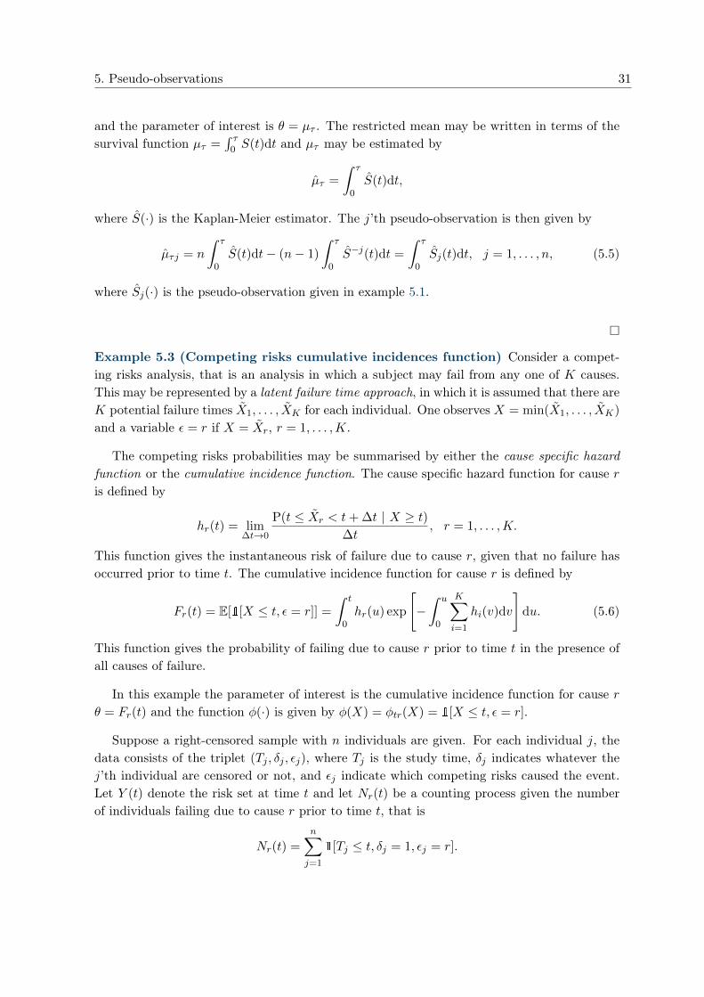
Example 5.3 (Competing risks cumulative incidences function) Consider a compet-ing risks analysis, that is an analysis in which a subject may fail from any one of K causes.This may be represented by a latent failure time approach, in which it is assumed that there areK potential failure times X1, . . . , XK for each individual. One observes X = min(X1, . . . , XK)
and a variable ε = r if X = Xr, r = 1, . . . ,K.
The competing risks probabilities may be summarised by either the cause specific hazardfunction or the cumulative incidence function. The cause specific hazard function for cause ris defined by
hr(t) = lim∆t→0
P(t ≤ Xr < t+ ∆t | X ≥ t)∆t
, r = 1, . . . ,K.
This function gives the instantaneous risk of failure due to cause r, given that no failure hasoccurred prior to time t. The cumulative incidence function for cause r is defined by
Fr(t) = E[1[X ≤ t, ε = r]] =
∫ t
0hr(u) exp
[−∫ u
0
K∑i=1
hi(v)dv
]du. (5.6)
This function gives the probability of failing due to cause r prior to time t in the presence ofall causes of failure.
In this example the parameter of interest is the cumulative incidence function for cause rθ = Fr(t) and the function φ(·) is given by φ(X) = φtr(X) = 1[X ≤ t, ε = r].
Suppose a right-censored sample with n individuals are given. For each individual j, thedata consists of the triplet (Tj , δj , εj), where Tj is the study time, δj indicates whatever thej’th individual are censored or not, and εj indicate which competing risks caused the event.Let Y (t) denote the risk set at time t and let Nr(t) be a counting process given the numberof individuals failing due to cause r prior to time t, that is
Nr(t) =n∑j=1
1[Tj ≤ t, δj = 1, εj = r].
32 5.1. Properties of the pseudo-observations
The cumulative incidence function (5.6) may be estimated by the Aalen-Johansen estimatorgiven by
Fr(t) =
∫ t
0
∏v<u
(1−
∑Kr=1 dNr(v)
Y (v)
)dHr(u),
where Hr(·) is the Nelson-Aalen estimator for the cumulative cause-r specified hazard functiongiven by
Hr(t) =
∫ t
0
dNr(u)
Y (u).
The Aalen-Johansen estimator is an approximately unbiased estimator of Fr(t) Andersen et al.[1993]. The j’th pseudo-observation corresponding to Fr(·) at time t0 is then given by
Fjr(t0) = nFr(t0)− (n− 1)F−jr (t0), r = 1, . . . ,K. (5.7)
�
Before any further comments on regression analysis with pseudo-observations, some generalproperties of the pseudo-observations are considered. In the following let Tj = min(Xj , Cj)
be the study time for individual j and let δj = 1[Xj ≤ Cj ].
5.1 Properties of the pseudo-observations
Studies of the pseudo-observations and their properties have so far been restricted to the caseof the survival function (example 5.1), the restricted mean survival time (example 5.2), andthe competing risks cumulative incidence function (example 5.3).
In a study of pseudo-observations in the context of the jackknife method, Tukey [1958]conjectured that the pseudo-observations may be treated as though they are i.i.d. Graw et al.[2009] showed that this is indeed the case when the pseudo-observations are calculated basedon the competing risks cumulative incidence function and when n approaches infinity. Inthe case of no competing risks, the estimated cumulative incidence function Fr(t) reducesto 1 − S(t) Fleming and Harrington [1991] and hence the property of i.i.d. also holds forpseudo-observations defined for the survival function and the restricted mean survival time.The results have not yet been proven in a general setting. Furthermore, it follows directlyfrom the definition of the pseudo-observation and the unbiased assumption of θ that eachpseudo-observation is an (approximately) unbiased estimator of θ.
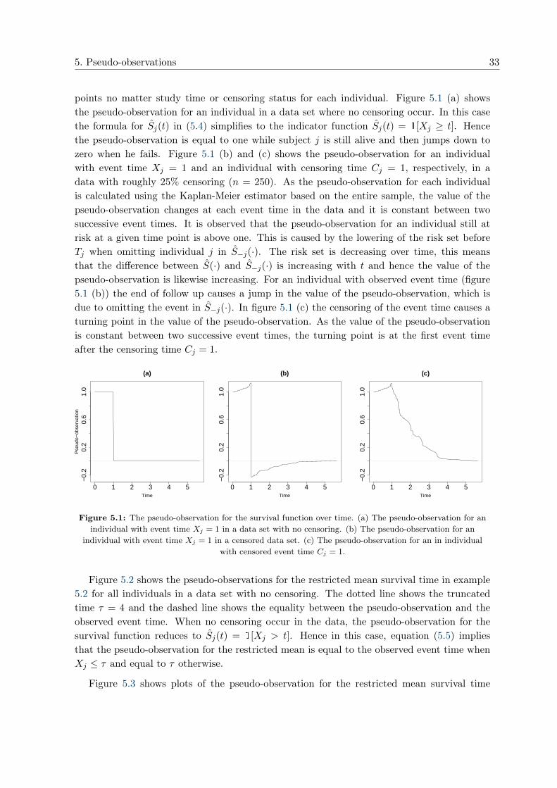
Figure 5.1 shows how the pseudo-observation for the survival function in example 5.1 maychange over time. Note that the pseudo-observation is defined for all individuals at all time
5. Pseudo-observations 33
points no matter study time or censoring status for each individual. Figure 5.1 (a) showsthe pseudo-observation for an individual in a data set where no censoring occur. In this casethe formula for Sj(t) in (5.4) simplifies to the indicator function Sj(t) = 1[Xj ≥ t]. Hencethe pseudo-observation is equal to one while subject j is still alive and then jumps down tozero when he fails. Figure 5.1 (b) and (c) shows the pseudo-observation for an individualwith event time Xj = 1 and an individual with censoring time Cj = 1, respectively, in adata with roughly 25% censoring (n = 250). As the pseudo-observation for each individualis calculated using the Kaplan-Meier estimator based on the entire sample, the value of thepseudo-observation changes at each event time in the data and it is constant between twosuccessive event times. It is observed that the pseudo-observation for an individual still atrisk at a given time point is above one. This is caused by the lowering of the risk set beforeTj when omitting individual j in S−j(·). The risk set is decreasing over time, this meansthat the difference between S(·) and S−j(·) is increasing with t and hence the value of thepseudo-observation is likewise increasing. For an individual with observed event time (figure5.1 (b)) the end of follow up causes a jump in the value of the pseudo-observation, which isdue to omitting the event in S−j(·). In figure 5.1 (c) the censoring of the event time causes aturning point in the value of the pseudo-observation. As the value of the pseudo-observationis constant between two successive event times, the turning point is at the first event timeafter the censoring time Cj = 1.
0 1 2 3 4 5
−0.
20.
20.
61.
0
(a)
Time
Pse
udo−
obse
rvat
ion
0 1 2 3 4 5
−0.
20.
20.
61.
0
(b)
Time
0 1 2 3 4 5
−0.
20.
20.
61.
0
(c)
Time
Figure 5.1: The pseudo-observation for the survival function over time. (a) The pseudo-observation for anindividual with event time Xj = 1 in a data set with no censoring. (b) The pseudo-observation for an
individual with event time Xj = 1 in a censored data set. (c) The pseudo-observation for an in individualwith censored event time Cj = 1.
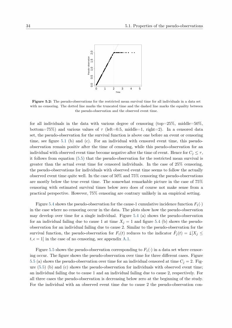
Figure 5.2 shows the pseudo-observations for the restricted mean survival time in example5.2 for all individuals in a data set with no censoring. The dotted line shows the truncatedtime τ = 4 and the dashed line shows the equality between the pseudo-observation and theobserved event time. When no censoring occur in the data, the pseudo-observation for thesurvival function reduces to Sj(t) = 1[Xj > t]. Hence in this case, equation (5.5) impliesthat the pseudo-observation for the restricted mean is equal to the observed event time whenXj ≤ τ and equal to τ otherwise.
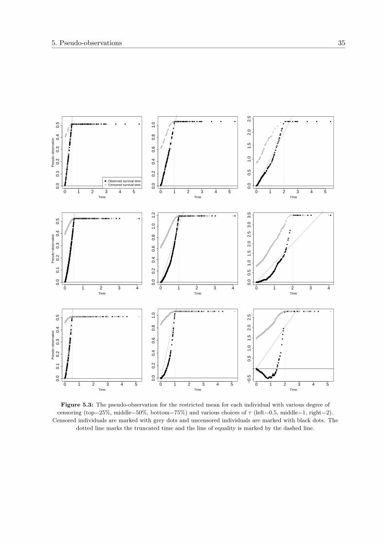
Figure 5.3 shows plots of the pseudo-observation for the restricted mean survival time
34 5.1. Properties of the pseudo-observations
●●●●●●●●●●●●●●●●●●●●●●●●●●●●●●●●●●●●●●●●●●●●●●●●●●●●●●●●●●●●●●●●●●●●●●●●●●●●●●●●●●●●●●●●●●●●●●●●●●●●●●●●●●●●●●●●●●●●●●●●●●●●●●●●●●●●●●●●●●●
●●●●●
●●●●●●●●●
●●●●●●●●●●●●●●
●●●●●●●●●●●●●●●●●●●●●●
●●
●●
●●
●●●●●●●●●●●●●●●●
●●●●●
●●
●●●●●●● ●●●●● ●●●●●● ●●●● ● ● ● ● ●● ● ● ●
0 1 2 3 4 50.
00.
51.
01.
52.
0Time
Pse
udo−
obse
rvat
ion
Figure 5.2: The pseudo-observations for the restricted mean survival time for all individuals in a data setwith no censoring. The dotted line marks the truncated time and the dashed line marks the equality between
the pseudo-observation and the observed event time.
for all individuals in the data with various degree of censoring (top=25%, middle=50%,bottom=75%) and various values of τ (left=0.5, middle=1, right=2). In a censored dataset, the pseudo-observation for the survival function is above one before an event or censoringtime, see figure 5.1 (b) and (c). For an individual with censored event time, this pseudo-observation remain positiv after the time of censoring, while this pseudo-observation for anindividual with observed event time become negative after the time of event. Hence for Cj ≤ τ ,it follows from equation (5.5) that the pseudo-observation for the restricted mean survival isgreater than the actual event time for censored individuals. In the case of 25% censoring,the pseudo-observations for individuals with observed event time seems to follow the actuallyobserved event time quite well. In the case of 50% and 75% censoring the pseudo-observationsare mostly below the true event time. The somewhat remarkable picture in the case of 75%
censoring with estimated survival times below zero does of course not make sense from apractical perspective. However, 75% censoring are contrary unlikely in an empirical setting.
Figure 5.4 shows the pseudo-observation for the cause-1 cumulative incidence function F1(·)in the case where no censoring occur in the data. The plots show how the pseudo-observationmay develop over time for a single individual. Figure 5.4 (a) shows the pseudo-observationfor an individual failing due to cause 1 at time Xj = 1 and figure 5.4 (b) shows the pseudo-observation for an individual failing due to cause 2. Similar to the pseudo-observation for thesurvival function, the pseudo-observation for F1(t) reduces to the indicator Fj(t) = 1[Xj ≤t, ε = 1] in the case of no censoring, see appendix A.1.
Figure 5.5 shows the pseudo-observation corresponding to F1(·) in a data set where censor-ing occur. The figure shows the pseudo-observation over time for three different cases. Figure5.5 (a) shows the pseudo-observation over time for an individual censored at time Cj = 2. Fig-ure (5.5) (b) and (c) shows the pseudo-observation for individuals with observed event time;an individual failing due to cause 1 and an individual failing due to cause 2, respectively. Forall three cases the pseudo-observation is decreasing below zero at the beginning of the study.For the individual with an observed event time due to cause 2 the pseudo-observation con-
5. Pseudo-observations 35
●●●●●●●●●●
●
●●
●
●
●
●●
●●●
●●
●●
●●
●
●●
●
●●●●
●
●
●
●
●●●
●●●
●●●●●
●
●
●
●●●●
●●
●●●●●●
●●
●●●●●
●
●●●●●
●
●●
●
●
●●
●
●●●●●●●●●●●●●●●
●
●
●
●●
●●●
●
●
●●●●●
●●
●●●
●●
●●●
●
●●●
●
●
●●●●●●●●●●●●●●●●●●●●●●●●●●●●●●●●●●●●●●●●●●●●●●●●●●●●●●●●●●●●●●●●●●●●●●●●●●●●●●●●●●●● ●●●●●●●●●●●●●●● ● ●● ● ●●●●●● ● ● ● ● ● ● ● ● ●
0 1 2 3 4 5
0.0
0.1
0.2
0.3
0.4
0.5
Time
Pse
udo−
obse
rvat
ion
●
●
Observed survival timeCensored survival time ●●●●●
●●●●●
●
●●
●
●
●
●●
●●●
●●
●●
●●
●
●●
●
●●●●
●
●●
●
●●●●●●●●●●●●●
●
●●●●
●●
●●●●●●
●●
●●●●●
●
●●●●●
●
●●●
●
●●
●
●●●●●●●●●●●●●●●
●
●●
●●
●●●
●
●●●●●●
●●
●●●
●●
●●●●●●●
●
●
●
●●●●
●
●●
●●●
●
●●●●●●
●●●●●●
●●●
●
●
●
●●
●●●
●●
●●●●●
●
●●●
●
●●●
●
●●
●
●
●●
●
●●
●
●●●●●●●●●●●●●●●●●●●●●●● ●●●●●●●●●●●●●●● ● ●● ● ●●●●●● ● ● ● ● ● ● ● ● ●
0 1 2 3 4 5
0.0
0.2
0.4
0.6
0.8
1.0
Time
●●●●●●●●●●
●
●●
●
●
●
●●
●●●
●●
●●
●●
●
●●
●
●●●●
●
●●
●
●●●●●●●●●●●●●
●
●●●●
●●
●●●●●●
●●
●●●●●
●
●●●●●
●
●●●
●
●●●●●●●●●●●●●●●●●●
●
●●
●●
●●●
●
●●●●●●
●●
●●●
●●
●●●●●●●
●
●
●
●●●●●
●●
●●●
●
●●●●●●●●●●●●
●●●
●
●
●
●●
●●●
●●
●●●●●
●
●●●
●
●●●
●
●●
●
●
●●
●
●●
●●
●●
●
●●●
●
●●●●●●
●
●
●
●●●
●
●
●
●
●
●
●
●
●
●●
●●
●
●
●
●●
●
●● ● ●●●●●● ● ● ● ● ● ● ● ● ●
0 1 2 3 4 5
0.0
0.5
1.0
1.5
2.0
2.5
Time
●●●●●●●●
●●●
●●
●
●●
●●●
●●●
●●●
●●●
●●●●●
●
●●
●
●
●●●●●
●
●
●●●
●
●
●●●
●●●●
●●
●
●
●
●
●●
●
●
●
●
●
●
●
●
●●
●
●●
●●●●
●
●●●●
●
●
●●●●
●●
●●●
●●●●
●●●
●
●
●
●●●●
●
●●
●●
●●
●●●
●●
●
●
●
●●●●
●
●●●
●●●
●
●●●●
●
●●
●●●
●
●
●●●
●●●
●
●●
●●●
●
●
●●●
●
●
●●●
●
●
●
●●●
●●
●
●●●●
●
●●●
●
●●●●●
●●
●
●
●●●●
●
●
●●
●●
●●
●
●●
●●
●
●
●
●
●
●●
●●
●
●
●
●
●●
●
●
●
●
●●●
●
●●
●●●
●
●●
●
●
●
●●
●
●
●●●●●●●●●●
●
●●
●
●●●●●
●●●
●
●●●
●●●
●
●●●
●
●●
●●
●
●
●
●●●●●
●●●●
●
●
●●●●●
●●
●●
●●●●●
●●●
●
●●
●●
●●
●●●
●●●
●
●●●
●
●
●●
●●
●●
●
●
●
●
●●
●
●
●●●
●●●
●●
●
●
●
●●
●
●
●●●
●
●●●
●●
●
●●
●●
●
●
●
●
●
●
●●●●●●
●
●●●
●●
●
●●●
●●●
●
●
●●
●
●
●●●
●
●●
●●●●
●
●●●
●●
●●
●
●●
●●
●●●●
●●●
●
●●●
●
●●●
●
●●
●
●●●
●
●●
●
●●
●●●●
●
●●
●
●●
●
●
●
●●●●●
●
●
●
●●
●
●
●●●
●●
●●
●
●●●●
●●
●
●
●●
●
●●●●●●●
●
●●●●
●●●●●●●
●●●
●●
●●
●
●●
●
●●●
●
●
●●●●
●
●●
●●●●
●
●●
●
●
●
●●●●
●●●
●●
●
●
●
●●●
●●
●●
●●●
●
●
●
●●●
●
●●
●●
●●●●●
●●
●●
●●
●
●●
●
●
●●
●
●
●●
●●●
●●
●●
●
●
●
●
●●
●●●●●●
●
●
●●●●●●●●●●●●●●●●●●●●●●●●●●●●●●●●●●●●●●●●●●●●●●●●●●●●●●●●●●●●●●●●●●●●●●●●●●●●●●●●●●●●●●●●●●●●●●●●●●●●●●●●●●●●●●●●●●●●●●●●●●●●●●●●●●●●●●●●●●●●●●●●●●●●●●●●●●●●●●●●●●●●●●●●●●●●●●●●●●●●●●●●●●●●●●●●●●●●●●●●●●●●●●●●●●●●●●●●●●●●●●●●●●●●●●●●●●●●●●●●●●●●●●●●●●●●●●●●●●●●●●●●●●●●●●●●●●●●●●●●●●●●●●●●●●●●●●●●●●●●●●●●●●●●●●●●●●●●●●●●●●●●●●●●●● ●●●●●●● ● ●●● ●●●● ●●● ●●● ●● ● ●● ●● ● ●
0 1 2 3 4
0.0
0.1
0.2
0.3
0.4
0.5
Time
Pse
udo−
obse
rvat
ion
●●●●●●●●
●●●
●●
●
●●
●●●
●●●
●●●
●●●
●●●●●
●
●●
●
●
●●●●●
●
●
●●●
●
●
●●●
●●●●
●●
●
●
●
●
●●
●
●
●
●
●
●
●
●
●●
●
●●
●●●●
●
●●●●
●
●
●●●●
●●
●●●
●●●●
●●●
●
●
●
●●●●
●
●●
●●
●●
●●●
●●
●
●
●
●●●●
●
●●●
●●●
●
●●●●
●
●●
●●●
●
●
●●●
●●●
●
●●
●●●
●
●
●●●
●
●
●●●
●
●
●
●●●
●●
●
●●●●
●
●●●
●
●●●●●
●●
●
●
●●●●
●
●
●●
●●
●●
●
●●
●●
●
●
●
●
●
●●
●●
●
●
●
●
●●
●
●
●
●
●●●
●
●●
●●●
●
●●
●
●
●
●●
●
●
●●●●●●●●●●
●
●●
●
●●●●●
●●●
●
●●●
●●●
●
●●●
●
●●
●●
●
●
●
●●●●●
●●●●
●
●
●●●●●
●●
●●
●●●●●
●●●
●
●●
●●
●●
●●●
●●●
●
●●●
●
●
●●
●●
●●
●
●
●
●
●●
●
●
●●●
●●●
●●
●
●
●
●●
●
●
●●●
●
●●●
●●
●
●●
●●
●
●
●
●
●
●
●●●●●●
●
●●●
●●
●
●●●
●●●
●
●
●●
●
●
●●●
●
●●
●●●●
●
●●●
●●
●●
●
●●
●●
●●●●
●●●
●
●●●
●
●●●
●
●●
●
●●●
●
●●
●
●●
●●●●
●
●●
●
●●
●
●
●
●●●●●
●
●
●
●●
●
●
●●●
●●
●●
●
●●●●
●●
●
●
●●
●
●●●●●●●
●
●●●●
●●●●●●●
●●●
●●
●●
●
●●
●
●●●
●
●
●●●●
●
●●
●●●●
●
●●
●
●
●
●●●●
●●●
●●
●
●
●
●●●
●●
●●
●●●
●
●
●
●●●
●
●●
●●
●●●●●
●●
●●
●●
●
●●
●
●
●●
●
●
●●
●●●
●●
●●
●
●
●
●
●●
●●●●●●
●
●
●●●●●●
●●●
●
●
●●●●
●●
●
●
●
●●
●
●
●
●●●●
●●
●●●
●●
●
●●
●●
●
●●
●●●●
●
●●
●
●
●●
●●
●
●●●●
●
●●●
●
●●●●
●●
●●●●
●
●●
●
●●
●●●
●
●
●
●
●
●
●●●●
●
●●●●●
●
●
●
●●
●●
●●
●●
●●
●
●●●
●●
●●
●●
●●
●
●
●●
●
●
●
●●
●
●
●
●
●●●●
●●
●●
●
●●●
●
●●
●●
●●●●●
●
●
●
●
●
●
●
●
●
●●
●●
●
●
●●
●
●●
●
●
●
●●●
●
●
●
●
●
●
●●●
●
●
●●●●
●●●●●
●
●
●
●
●●●●●
●
●●
●●●●●●●●●●●●●●●●●●●●●●●●●●●●●●●●●●●●●●●●●●●●●●●●●●●●●●●●●●●●●●●●●●●●●●●●●●●●●●●●●●●●●●●●●●●●●●●●●●●●●●●●●●●●●● ●●●●●●● ● ●●● ●●●● ●●● ●●● ●● ● ●● ●● ● ●
0 1 2 3 4
0.0
0.2
0.4
0.6
0.8
1.0
1.2
Time
●●●●●●●●
●●●
●●
●
●●
●●●
●●●
●●●
●●●
●●●●●
●
●●
●
●
●●●●●
●
●
●●●
●
●
●●●
●●●●
●●
●
●
●
●
●●
●
●
●
●
●
●
●
●
●●
●
●●
●●●●
●
●●●●
●
●
●●●●
●●
●●●
●●●●
●●●
●
●
●
●●●●
●
●●
●●
●●
●●●
●●
●
●
●
●●●●
●
●●●
●●●
●
●●●●
●
●●
●●●
●
●
●●●
●●●
●
●●
●●●
●
●
●●●
●
●
●●●
●
●
●
●●●
●●
●
●●●●
●
●●●
●
●●●●●
●●
●
●
●●●●
●
●
●●
●●
●●
●
●●
●●
●
●
●
●
●
●●
●●
●
●
●
●
●●
●
●
●
●
●●●
●
●●
●●●
●
●●
●
●
●
●●
●
●
●●●●●●●●●●
●
●●
●
●●●●●
●●●
●
●●●
●●●
●
●●●
●
●●
●●
●
●
●
●●●●●
●●●●
●
●
●●●●●
●●
●●
●●●●●
●●●
●
●●
●●
●●
●●●
●●●
●
●●●
●
●
●●
●●
●●
●
●
●
●
●●
●
●
●●●
●●●
●●
●
●
●
●●
●
●
●●●
●
●●●
●●
●
●●
●●
●
●
●
●
●
●
●●●●●●
●
●●●
●●
●
●●●
●●●
●
●
●●
●
●
●●●
●
●●
●●●●
●
●●●
●●
●●
●
●●
●●
●●●●
●●●
●
●●●
●
●●●
●
●●
●
●●●
●
●●
●
●●
●●●●
●
●●
●
●●
●
●
●
●●●●●
●
●
●
●●
●
●
●●●
●●
●●
●
●●●●
●●
●
●
●●
●
●●●●●●●
●
●●●●
●●●●●●●
●●●
●●
●●
●
●●
●
●●●
●
●
●●●●
●
●●
●●●●
●
●●
●
●
●
●●●●
●●●
●●
●
●
●
●●●
●●
●●
●●●
●
●
●
●●●
●
●●
●●
●●●●●
●●
●●
●●
●
●●
●
●
●●
●
●
●●
●●●
●●
●●
●
●
●
●
●●
●●●●●●
●
●
●●●●●●
●●●
●
●
●●●●
●●
●
●
●
●●
●
●
●
●●●●
●●
●●●
●●
●
●●
●●
●
●●
●●●●
●
●●
●
●
●●
●●
●
●●●●
●
●●●
●
●●●●
●●
●●●●
●
●●
●
●●
●●●
●
●
●
●
●
●
●●●●
●
●●●●●
●
●
●
●●
●●
●●
●●
●●
●
●●●
●●
●●
●●
●●
●
●
●●
●
●
●
●●
●
●
●
●
●●●●
●●
●●
●
●●●
●
●●
●●
●●●●●
●
●
●
●
●
●
●
●
●
●●
●●
●
●
●●
●
●●
●
●●
●●●
●
●
●
●
●
●
●●●
●
●●●●●
●●●●●
●
●
●
●
●●●●●
●
●●
●
●●
●
●●●●
●●
●
●
●●
●
●●●
●
●●●
●
●
●
●●●●●
●
●●
●●
●●●
●●●●
●
●
●●
●
●●
●●●
●
●●●●
●●●●●
●
●
●●
●
●
●●●
●●
●●
●
●
●●●●●
●
●
●
●●
●
●●●
●●
●
●
●
●
●
●
●
●●
●
●
●
●
●
●
●
●
●
●
●●
●
●
● ● ●●● ●●●● ●●● ●●● ●● ● ●● ●● ● ●
0 1 2 3 4
0.0
0.5
1.0
1.5
2.0
2.5
3.0
3.5
Time
●●●●
●●●
●●
●●●●●●●●
●
●●●
●
●●●●●●
●
●
●
●●●●●●●
●
●●●●●
●
●●●●
●●●
●●●
●
●
●
●●●●●●
●●
●●●
●
●●●
●
●●
●
●
●●
●●
●
●●●●●
●
●
●●
●
●
●●●●●●
●●●
●
●
●●●●●●
●
●
●●
●●●●●
●
●●
●
●●●
●●
●●●●●
●
●●●
●
●●
●●●●
●●
●
●
●
●
●
●●●●●●●●
●
●●●●
●●
●●●●●●●
●
●●●●
●●
●
●
●●●●●
●
●●
●
●●
●
●●●●●●●
●
●
●
●●
●●●
●
●
●●●●●●
●
●●●●●
●●●
●●●●●●●●
●
●●●●●
●
●●●●●●●●
●
●●●
●
●●●●
●
●●●
●●
●●●●●●●●●●
●
●●●
●
●●
●
●●
●
●●●
●
●●●●
●
●●●●●●●●●●●●
●
●
●
●●●●
●
●●●●●●●
●
●●●●●●●●
●●
●●●●
●
●●
●
●
●●
●●●
●●
●●●●
●
●●●
●
●●
●
●●
●●
●●●●
●
●●
●
●●●
●
●●●
●
●●●●●●●●
●
●●●●●●●●●●
●
●
●
●
●●
●
●
●
●
●●●●●●●●●●●
●●
●●●
●●
●●●●●●●
●
●●●●●●●●●●
●●
●●●●●●●●●●●●●
●
●●●●●●●●●●●●●●●●●
●●
●●●●●●
●
●●
●●●●●●●●●●●●●●●●●●●●●●●●●●●●●●●●●●●●●●●●●●●●●●●●●●●●●●●●●●●●●●●●●●●●●●●●●●●●●●●●●●●●●●●●●●●●●●●●●●●●●●●●●●●●●●●●●●●●●●●●●●●●●●●●●●●●●●●●●●●●●●●●●●●●●●●●●●●●●●●●●●●●●●●●●●●●●●●●●●●●●●●●●●●●●●●●●●●●●●●●●●●●●●●●●●●●●●●●●●●●●●●●●●●●●●●●●●●●●●●●●●●●●●●●●●●●●●●●●●●●●●●●●●●●●●●●●●●●●●●●●●●●●●●●●●●●●●●●●●●●●●●●●●●●●●●●●●●●●●●●●●●●●●●●●●●●●●●●●●●●●●●●●●●●●●●●●●●●●●●●●●●●●●●●●●●●●●●●●●●●●●●●●●●●●●●●●●●●●●●●●●●●●●●●●●●●●●●●●●●●●●●●●●●●●●●●●●●●●●●●●●●●●●●●●●●●●●●●●●●●●●●●●●●●●●●●●●●●●●●● ●●●●● ●●● ●●●● ●● ●●●● ● ●●●●●● ● ●● ● ●
0 1 2 3 4 5
0.0
0.1
0.2
0.3
0.4
0.5
Time
Pse
udo−
obse
rvat
ion
●●●●
●●●
●●
●●●●●●●●
●
●●●
●
●●●●●●
●
●
●
●●●●●●●
●
●●●●●
●
●●●●
●●●
●●●
●
●
●
●●●●●●
●●
●●●
●
●●●
●
●●
●
●
●●
●●
●
●●●●●
●
●
●●
●
●
●●●●●●
●●●
●
●
●●●●●●
●
●
●●
●●●●●
●
●●
●
●●●
●●
●●●●●
●
●●●
●
●●
●●●●
●●
●
●
●
●
●
●●●●●●●●
●
●●●●
●●
●●●●●●●
●
●●●●
●●
●
●
●●●●●
●
●●
●
●●
●
●●●●●●●
●
●
●
●●
●●●
●
●
●●●●●●
●
●●●●●
●●●
●●●●●●●●
●
●●●●●
●
●●●●●●●●
●
●●●
●
●●●●
●
●●●
●●
●●●●●●●●●●
●
●●●
●
●●
●
●●
●
●●●
●
●●●●
●
●●●●●●●●●●●●
●
●
●
●●●●
●
●●●●●●●
●
●●●●●●●●
●●
●●●●
●
●●
●
●
●●
●●●
●●
●●●●
●
●●●
●
●●
●
●●
●●
●●●●
●
●●
●
●●●
●
●●●
●
●●●●●●●●
●
●●●●●●●●●●
●
●
●
●
●●
●
●
●
●
●●●●●●●●●●●
●●
●●●
●●
●●●●●●●
●
●●●●●●●●●●
●●
●●●●●●●●●●●●●
●
●●●●●●●●●●●●●●●●●
●●
●●●●●●
●●●
●●●●●●●●●●●●●●●●●●
●
●●
●
●
●●
●
●
●●●●●
●
●●●●
●●●
●●●●●
●
●●●●●●●●●●●●●
●
●●●●●●●
●
●●
●
●●●●●
●
●
●●
●●●●●
●
●●●●
●
●●
●
●●●●
●●
●●●●●●●●●●
●
●
●
●●●●●●●●
●●
●●
●
●●●●
●●
●●●●●●●
●●●
●●●●●
●
●●●
●
●●●●●●●●●●●●●●●●●●●●●●●●●●
●
●●●●●●●●●●
●
●●●
●
●●●●●●●
●●●
●●●
●●
●●
●
●
●
●●
●
●●
●
●●
●
●●●●●●●●●●●
●
●●●●●
●
●●●
●
●●●●●●
●
●●
●
●●●●●●●●●●●●●●●●●●●●●●●●●●●●●●●●●●●●●●●●●●●●●●●●●●●●●●●●●●●●●●●●●●●●●●●●●●●●●●●●●●●●●●●●●●●●●●●●●●●●●●●●●●●●●●●●●●●●●●●●●●●●●●●●●●●●●●●●●●●●●●●●●●●●●●●●●●●●●●●●●●●●●●●●●●●●●●●●●●●●●●●●●●●●●●●●●●●●●●●●●●●●●●●●●●●●●●●●●●●●●●●●● ●●●●● ●●● ●●●● ●● ●●●● ● ●●●●●● ● ●● ● ●
0 1 2 3 4 5
0.0
0.2
0.4
0.6
0.8
1.0
Time
●●●●
●●●
●●
●●●●●●●●
●
●●●
●
●●●●●●
●
●
●
●●●●●●●
●
●●●●●
●
●●●●
●●●
●●●
●
●
●
●●●●●●
●●
●●●
●
●●●
●
●●
●
●
●●
●●
●
●●●●●
●
●
●●
●
●
●●●●●●
●●●
●
●
●●●●●●
●
●
●●
●●●●●
●
●●
●
●●●
●●
●●●●●
●
●●●
●
●●
●●●●
●●
●
●
●
●
●
●●●●●●●●
●
●●●●
●●
●●●●●●●
●
●●●●
●●
●
●
●●●●●
●
●●
●
●●
●
●●●●●●●
●
●
●
●●
●●●
●
●
●●●●●●
●
●●●●●
●●●
●●●●●●●●
●
●●●●●
●
●●●●●●●●
●
●●●
●
●●●●
●
●●●
●●
●●●●●●●●●●
●
●●●
●
●●
●
●●
●
●●●
●
●●●●
●
●●●●●●●●●●●●
●
●
●
●●●●
●
●●●●●●●
●
●●●●●●●●
●●
●●●●
●
●●
●
●
●●
●●●
●●
●●●●
●
●●●
●
●●
●
●●
●●
●●●●
●
●●
●
●●●
●
●●●
●
●●●●●●●●
●
●●●●●●●●●●
●
●
●
●
●●
●
●
●
●
●●●●●●●●●●●
●●
●●●
●●
●●●●●●●
●
●●●●●●●●●●
●●
●●●●●●●●●●●●●
●
●●●●●●●●●●●●●●●●●
●●
●●●●●●
●●●
●●●●●●●●●●●●●●●●●●
●
●●
●
●
●●
●
●
●●●●●
●
●●●●
●●●
●●●●●
●
●●●●●●●●●●●●●
●
●●●●●●●
●
●●
●
●●●●●
●
●
●●
●●●●●
●
●●●●
●
●●
●
●●●●
●●
●●●●●●●●●●
●
●
●
●●●●●●●●
●●
●●
●
●●●●
●●
●●●●●●●
●●●
●●●●●
●
●●●
●
●●●●●●●●●●●●●●●●●●●●●●●●●●
●
●●●●●●●●●●
●
●●●
●
●●●●●●●
●●●
●●●
●●
●●
●
●
●
●●
●
●●
●
●●
●
●●●●●●●●●●●
●
●●●●●
●
●●●
●
●●●●●●
●
●●
●
●●●●●●●●●●●
●
●●●
●
●
●
●
●
●●●●●●
●
●●●
●
●●●●●●
●
●
●
●●●
●
●●
●
●●●●●●
●
●●●●●●●●●
●
●●●●●
●●
●●●
●●
●●●●●●●●
●
●●●
●
●●●●●
●●●
●
●
●●●
●●
●
●
●●
●
●
●
●●●●●
●
●●●●●
●●
●●●
●
●
●●
●●●●●●●
●
●●●●
●
●
●
●●●
●
●●●●●●●●
●
●●●
●
●●●●●●
●
●●●●●●●
●
●●
●
●
●
●●●
●
●
●●●●●●●●●●●●●●●●●●●●●●●●●●●●●●●●●●●●● ●●●●● ●●● ●●●● ●● ●●●● ● ●●●●●● ● ●● ● ●
0 1 2 3 4 5−0.
50.
51.
01.
52.
02.
5
Time
Figure 5.3: The pseudo-observation for the restricted mean for each individual with various degree ofcensoring (top=25%, middle=50%, bottom=75%) and various choices of τ (left=0.5, middle=1, right=2).
Censored individuals are marked with grey dots and uncensored individuals are marked with black dots. Thedotted line marks the truncated time and the line of equality is marked by the dashed line.
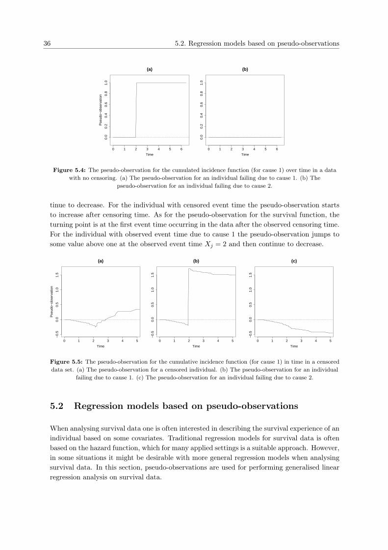
36 5.2. Regression models based on pseudo-observations
0 1 2 3 4 5 6
0.0
0.2
0.4
0.6
0.8
1.0
(a)
Time
Pse
udo−
obse
rvat
ion
0 1 2 3 4 5 6
0.0
0.2
0.4
0.6
0.8
1.0
(b)
Time
Figure 5.4: The pseudo-observation for the cumulated incidence function (for cause 1) over time in a datawith no censoring. (a) The pseudo-observation for an individual failing due to cause 1. (b) The
pseudo-observation for an individual failing due to cause 2.
tinue to decrease. For the individual with censored event time the pseudo-observation startsto increase after censoring time. As for the pseudo-observation for the survival function, theturning point is at the first event time occurring in the data after the observed censoring time.For the individual with observed event time due to cause 1 the pseudo-observation jumps tosome value above one at the observed event time Xj = 2 and then continue to decrease.
0 1 2 3 4 5
−0.
50.
00.
51.
01.
5
(a)
Time
Pse
udo−
obse
rvat
ion
0 1 2 3 4 5
−0.
50.
00.
51.
01.
5
(b)
Time
0 1 2 3 4 5
−0.
50.
00.
51.
01.
5
(c)
Time
Figure 5.5: The pseudo-observation for the cumulative incidence function (for cause 1) in time in a censoreddata set. (a) The pseudo-observation for a censored individual. (b) The pseudo-observation for an individual
failing due to cause 1. (c) The pseudo-observation for an individual failing due to cause 2.
5.2 Regression models based on pseudo-observations
When analysing survival data one is often interested in describing the survival experience of anindividual based on some covariates. Traditional regression models for survival data is oftenbased on the hazard function, which for many applied settings is a suitable approach. However,in some situations it might be desirable with more general regression models when analysingsurvival data. In this section, pseudo-observations are used for performing generalised linearregression analysis on survival data.
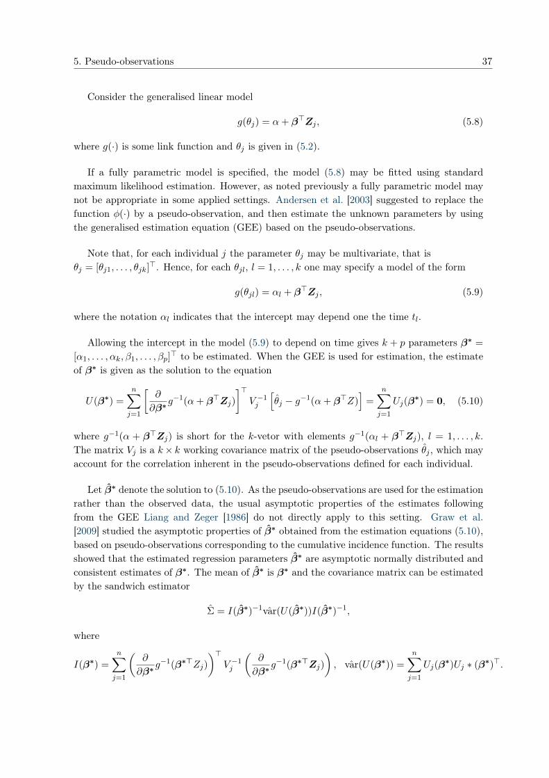
5. Pseudo-observations 37
Consider the generalised linear model
g(θj) = α+ β>Zj , (5.8)
where g(·) is some link function and θj is given in (5.2).
If a fully parametric model is specified, the model (5.8) may be fitted using standardmaximum likelihood estimation. However, as noted previously a fully parametric model maynot be appropriate in some applied settings. Andersen et al. [2003] suggested to replace thefunction φ(·) by a pseudo-observation, and then estimate the unknown parameters by usingthe generalised estimation equation (GEE) based on the pseudo-observations.
Note that, for each individual j the parameter θj may be multivariate, that isθj = [θj1, . . . , θjk]
>. Hence, for each θjl, l = 1, . . . , k one may specify a model of the form
g(θjl) = αl + β>Zj , (5.9)
where the notation αl indicates that the intercept may depend one the time tl.
Allowing the intercept in the model (5.9) to depend on time gives k + p parameters β∗ =
[α1, . . . , αk, β1, . . . , βp]> to be estimated. When the GEE is used for estimation, the estimate
of β∗ is given as the solution to the equation
U(β∗) =
n∑j=1
[∂
∂β∗g−1(α+ β>Zj)
]>V −1j
[θj − g−1(α+ β>Z)
]=
n∑j=1
Uj(β∗) = 0, (5.10)
where g−1(α + β>Zj) is short for the k-vetor with elements g−1(αl + β>Zj), l = 1, . . . , k.The matrix Vj is a k× k working covariance matrix of the pseudo-observations θj , which mayaccount for the correlation inherent in the pseudo-observations defined for each individual.
Let β∗ denote the solution to (5.10). As the pseudo-observations are used for the estimationrather than the observed data, the usual asymptotic properties of the estimates followingfrom the GEE Liang and Zeger [1986] do not directly apply to this setting. Graw et al.[2009] studied the asymptotic properties of β∗ obtained from the estimation equations (5.10),based on pseudo-observations corresponding to the cumulative incidence function. The resultsshowed that the estimated regression parameters β∗ are asymptotic normally distributed andconsistent estimates of β∗. The mean of β∗ is β∗ and the covariance matrix can be estimatedby the sandwich estimator
Σ = I(β∗)−1var(U(β∗))I(β∗)−1,
where
I(β∗) =n∑j=1
(∂
∂β∗g−1(β∗>Zj)
)>V −1j
(∂
∂β∗g−1(β∗>Zj)
), var(U(β∗)) =
n∑j=1
Uj(β∗)Uj ∗ (β∗)>.
38 5.2. Regression models based on pseudo-observations
The central part of the proof by Graw et al. [2009] is the finding that
E[Fjr(t)|Zj ] = g−1(β∗>Zj) + op(1), (5.11)
from which it follows that E[U(β∗)] = 0 for the true parameter β∗.
The results found by Graw et al. [2009] relies on two assumptions; the censoring times Cj isindependent of (Xj , δj ,Zj) and only time points t < τ such that SC(τ) > ν > 0 are considered.Here SC(·) denotes the survival function for the censoring distribution. By arguments as insection 5.1, the asymptotic results also holds for pseudo-observations corresponding to thesurvival function in example 5.1 and the restricted mean survival time in example 5.2. Theresults have not been proven in a general setting.
Notice that once the pseudo-observations have been calculated, one might consider a num-ber of models for analysing the data. However, the number and position of time points, forwhich the pseudo-observations are calculated, is a choice which must be made prior to theanalysis. One time point is enough to obtain estimates of the regression parameter, however,more times point may be more efficient for capturing the trend in the event distribution. Onechoice is to place the time points at equally spaced percentiles of the data. This choice willplace focus at regions with dense observed study times. Another choice is to place the timepoints at equally spaced study times, which will give a more varied representation of the ob-served data. However, the portion and position of censored data may also have some impactone the best suitable choice, cf. the plots in section 5.1. Klein and Andersen [2005] studied thenumber of time points in the context of competing risks. The results showed that increasingthe number of equally spaced time points did not have a significant impact on the precisionof the estimated regression parameters. Although this is confirmed in the example below, onemay conjecture that the best choice is related to the structure of the observed data.
Example 5.4 (Regression analysis on the survival function) Consider the pseudo-observations for the survival function in example 5.1. In that example the function φ(·)was given as the indicator function φt0(Xj) = 1[Xj > t0]. Suppose one wishes to performregression analysis on this function. The outcome of the regression analysis θj is then givenby S(t0|Zj). Choosing the link function as the cloglog-function, one gets the model
cloglog(S(t0|Zj)) = log (− log (S(t0|Zj)) , j = 1, . . . , n
= α0 + β>Zj , (5.12)
where α0 = log (H0(t0)) and H0(·) is a cumulative hazard function. The model (5.12) cor-respond to the Cox proportional hazards model as this model has survival function givenby
S(t|Zj) = S0(t)exp(β>Zj) = exp(−H0(t) exp
(β>Zj
)).
The model (5.12) may be extended to a multivariate model by simultaneous considering a gridof time points t1, . . . , tk. A model is then specified at each time point tl by
log (− log (S(tl|Zj))) = αl + β>Zj , l = 1, . . . , k, (5.13)
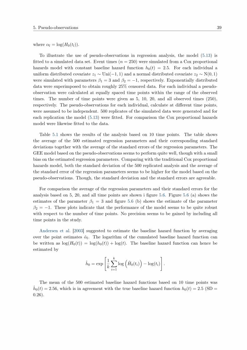
5. Pseudo-observations 39
where αl = log(H0(tl)).
To illustrate the use of pseudo-observations in regression analysis, the model (5.13) isfitted to a simulated data set. Event times (n = 250) were simulated from a Cox proportionalhazards model with constant baseline hazard function h0(t) = 2.5. For each individual auniform distributed covariate z1 ∼ Uni(−1, 1) and a normal distributed covariate z2 ∼ N(0, 1)
were simulated with parameters β1 = 3 and β2 = −1, respectively. Exponentially distributeddata were superimposed to obtain roughly 25% censored data. For each individual a pseudo-observation were calculated at equally spaced time points within the range of the observedtimes. The number of time points were given as 5, 10, 20, and all observed times (250),respectively. The pseudo-observations for each individual, calculate at different time points,were assumed to be independent. 500 replicates of the simulated data were generated and foreach replication the model (5.13) were fitted. For comparison the Cox proportional hazardsmodel were likewise fitted to the data.
Table 5.1 shows the results of the analysis based on 10 time points. The table showsthe average of the 500 estimated regression parameters and their corresponding standarddeviations together with the average of the standard errors of the regression parameters. TheGEE model based on the pseudo-observations seems to perform quite well, though with a smallbias on the estimated regression parameters. Comparing with the traditional Cox proportionalhazards model, both the standard deviation of the 500 replicated analysis and the average ofthe standard error of the regression parameters seems to be higher for the model based on thepseudo-observations. Though, the standard deviation and the standard errors are agreeable.
For comparison the average of the regression parameters and their standard errors for theanalysis based on 5, 20, and all time points are shown i figure 5.6. Figure 5.6 (a) shows theestimates of the parameter β1 = 3 and figure 5.6 (b) shows the estimate of the parameterβ2 = −1. These plots indicate that the performance of the model seems to be quite robustwith respect to the number of time points. No precision seems to be gained by including alltime points in the study.
Andersen et al. [2003] suggested to estimate the baseline hazard function by averagingover the point estimates αl. The logarithm of the cumulated baseline hazard function canbe written as log(H0(t)) = log(h0(t)) + log(t). The baseline hazard function can hence beestimated by
h0 = exp
[1
k
k∑i=1
log(H0(ti)
)− log(ti)
].
The mean of the 500 estimated baseline hazard functions based on 10 time points wash0(t) = 2.56, which is in agreement with the true baseline hazard function h0(t) = 2.5 (SD =
0.26).
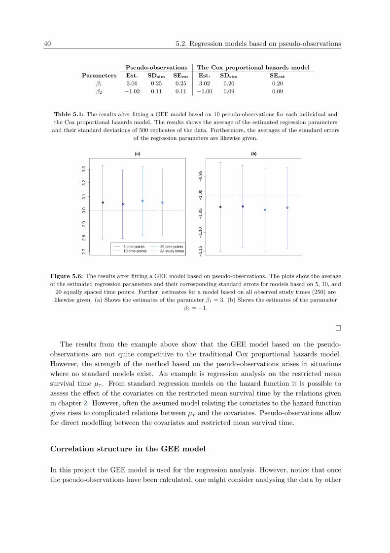
40 5.2. Regression models based on pseudo-observations
Pseudo-observations The Cox proportional hazards modelParameters Est. SDsim SEest Est. SDsim SEest
β1 3.06 0.25 0.25 3.02 0.20 0.20
β2 −1.02 0.11 0.11 −1.00 0.09 0.09
Table 5.1: The results after fitting a GEE model based on 10 pseudo-observations for each individual andthe Cox proportional hazards model. The results shows the average of the estimated regression parametersand their standard deviations of 500 replicates of the data. Furthermore, the averages of the standard errors
of the regression parameters are likewise given.
●●
●●
2.7
2.8
2.9
3.0
3.1
3.2
3.3
(a)
Est
imat
e
●●
●●
5 time points10 time points
20 time pointsAll study times
● ●
●
●
−1.
15−
1.10
−1.
05−
1.00
−0.
95
(b)
Est
imat
e
● ●
●
●
Figure 5.6: The results after fitting a GEE model based on pseudo-observations. The plots show the averageof the estimated regression parameters and their corresponding standard errors for models based on 5, 10, and20 equally spaced time points. Further, estimates for a model based on all observed study times (250) arelikewise given. (a) Shows the estimates of the parameter β1 = 3. (b) Shows the estimates of the parameter
β2 = −1.
�
The results from the example above show that the GEE model based on the pseudo-observations are not quite competitive to the traditional Cox proportional hazards model.However, the strength of the method based on the pseudo-observations arises in situationswhere no standard models exist. An example is regression analysis on the restricted meansurvival time µτ . From standard regression models on the hazard function it is possible toassess the effect of the covariates on the restricted mean survival time by the relations givenin chapter 2. However, often the assumed model relating the covariates to the hazard functiongives rises to complicated relations between µτ and the covariates. Pseudo-observations allowfor direct modelling between the covariates and restricted mean survival time.
Correlation structure in the GEE model
In this project the GEE model is used for the regression analysis. However, notice that oncethe pseudo-observations have been calculated, one might consider analysing the data by other
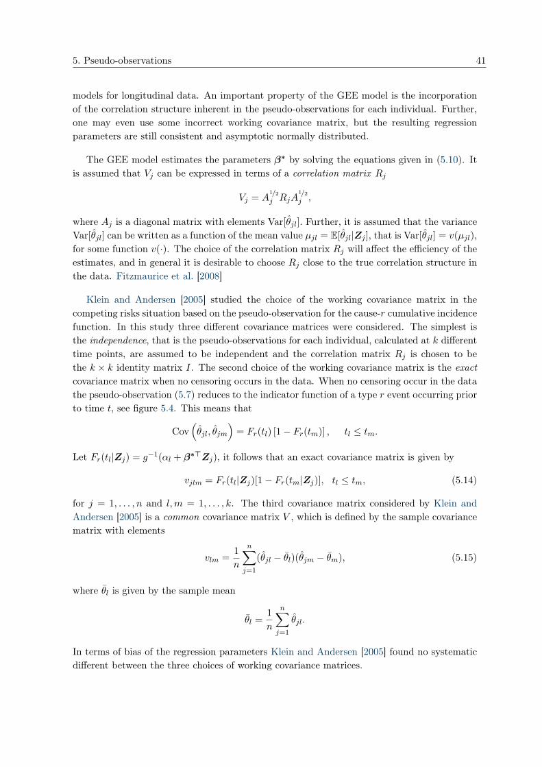
5. Pseudo-observations 41
models for longitudinal data. An important property of the GEE model is the incorporationof the correlation structure inherent in the pseudo-observations for each individual. Further,one may even use some incorrect working covariance matrix, but the resulting regressionparameters are still consistent and asymptotic normally distributed.
The GEE model estimates the parameters β∗ by solving the equations given in (5.10). Itis assumed that Vj can be expressed in terms of a correlation matrix Rj
Vj = A1/2j RjA
1/2j ,
where Aj is a diagonal matrix with elements Var[θjl]. Further, it is assumed that the varianceVar[θjl] can be written as a function of the mean value µjl = E[θjl|Zj ], that is Var[θjl] = v(µjl),for some function v(·). The choice of the correlation matrix Rj will affect the efficiency of theestimates, and in general it is desirable to choose Rj close to the true correlation structure inthe data. Fitzmaurice et al. [2008]
Klein and Andersen [2005] studied the choice of the working covariance matrix in thecompeting risks situation based on the pseudo-observation for the cause-r cumulative incidencefunction. In this study three different covariance matrices were considered. The simplest isthe independence, that is the pseudo-observations for each individual, calculated at k differenttime points, are assumed to be independent and the correlation matrix Rj is chosen to bethe k × k identity matrix I. The second choice of the working covariance matrix is the exactcovariance matrix when no censoring occurs in the data. When no censoring occur in the datathe pseudo-observation (5.7) reduces to the indicator function of a type r event occurring priorto time t, see figure 5.4. This means that
Cov(θjl, θjm
)= Fr(tl) [1− Fr(tm)] , tl ≤ tm.
Let Fr(tl|Zj) = g−1(αl + β∗>Zj), it follows that an exact covariance matrix is given by
vjlm = Fr(tl|Zj)[1− Fr(tm|Zj)], tl ≤ tm, (5.14)
for j = 1, . . . , n and l,m = 1, . . . , k. The third covariance matrix considered by Klein andAndersen [2005] is a common covariance matrix V , which is defined by the sample covariancematrix with elements
vlm =1
n
n∑j=1
(θjl − θl)(θjm − θm), (5.15)
where θl is given by the sample mean
θl =1
n
n∑j=1
θjl.
In terms of bias of the regression parameters Klein and Andersen [2005] found no systematicdifferent between the three choices of working covariance matrices.
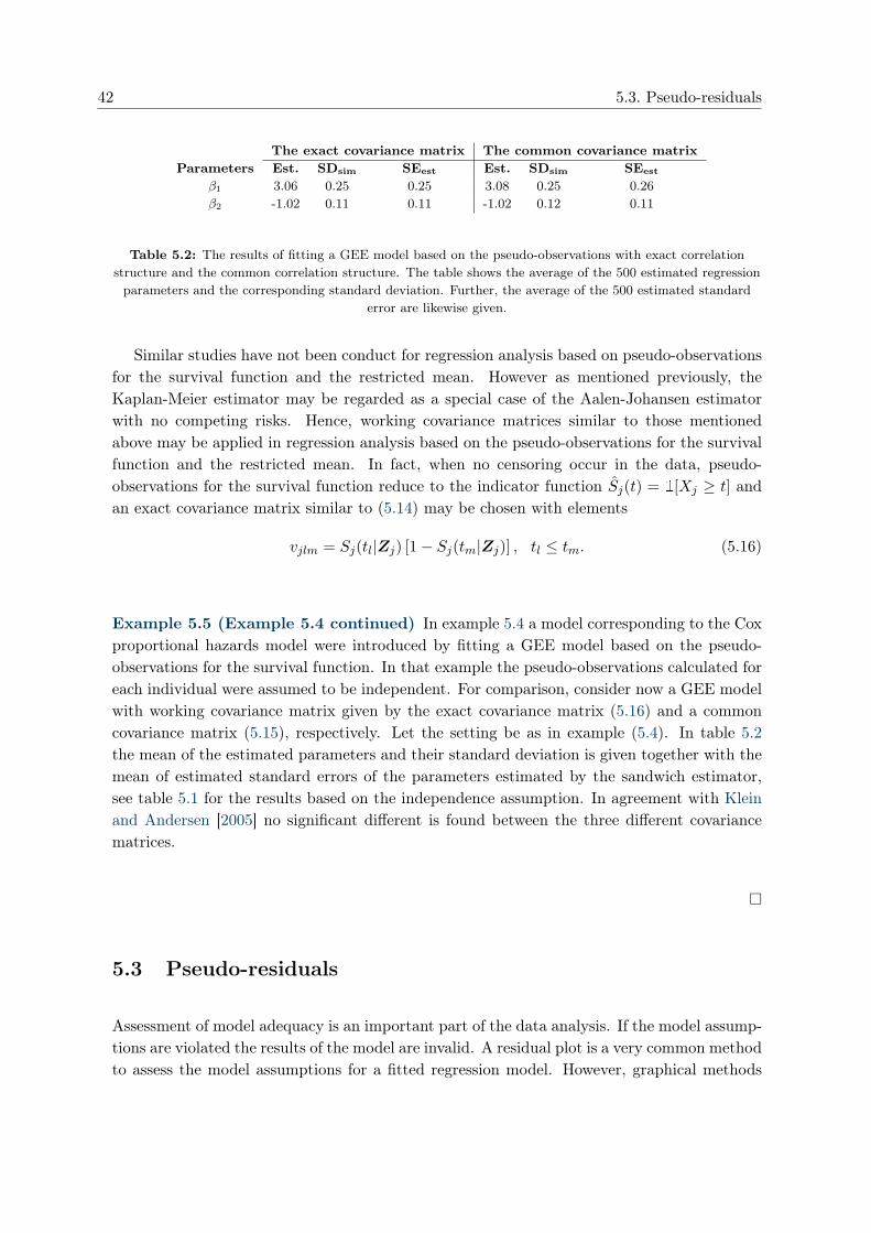
42 5.3. Pseudo-residuals
The exact covariance matrix The common covariance matrixParameters Est. SDsim SEest Est. SDsim SEest
β1 3.06 0.25 0.25 3.08 0.25 0.26β2 -1.02 0.11 0.11 -1.02 0.12 0.11
Table 5.2: The results of fitting a GEE model based on the pseudo-observations with exact correlationstructure and the common correlation structure. The table shows the average of the 500 estimated regressionparameters and the corresponding standard deviation. Further, the average of the 500 estimated standard
error are likewise given.
Similar studies have not been conduct for regression analysis based on pseudo-observationsfor the survival function and the restricted mean. However as mentioned previously, theKaplan-Meier estimator may be regarded as a special case of the Aalen-Johansen estimatorwith no competing risks. Hence, working covariance matrices similar to those mentionedabove may be applied in regression analysis based on the pseudo-observations for the survivalfunction and the restricted mean. In fact, when no censoring occur in the data, pseudo-observations for the survival function reduce to the indicator function Sj(t) = 1[Xj ≥ t] andan exact covariance matrix similar to (5.14) may be chosen with elements
vjlm = Sj(tl|Zj) [1− Sj(tm|Zj)] , tl ≤ tm. (5.16)
Example 5.5 (Example 5.4 continued) In example 5.4 a model corresponding to the Coxproportional hazards model were introduced by fitting a GEE model based on the pseudo-observations for the survival function. In that example the pseudo-observations calculated foreach individual were assumed to be independent. For comparison, consider now a GEE modelwith working covariance matrix given by the exact covariance matrix (5.16) and a commoncovariance matrix (5.15), respectively. Let the setting be as in example (5.4). In table 5.2the mean of the estimated parameters and their standard deviation is given together with themean of estimated standard errors of the parameters estimated by the sandwich estimator,see table 5.1 for the results based on the independence assumption. In agreement with Kleinand Andersen [2005] no significant different is found between the three different covariancematrices.
�
5.3 Pseudo-residuals
Assessment of model adequacy is an important part of the data analysis. If the model assump-tions are violated the results of the model are invalid. A residual plot is a very common methodto assess the model assumptions for a fitted regression model. However, graphical methods
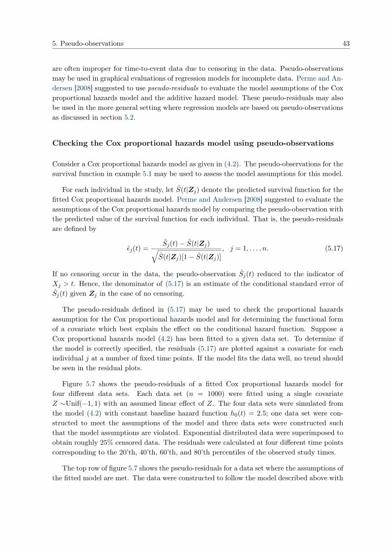
5. Pseudo-observations 43
are often improper for time-to-event data due to censoring in the data. Pseudo-observationsmay be used in graphical evaluations of regression models for incomplete data. Perme and An-dersen [2008] suggested to use pseudo-residuals to evaluate the model assumptions of the Coxproportional hazards model and the additive hazard model. These pseudo-residuals may alsobe used in the more general setting where regression models are based on pseudo-observationsas discussed in section 5.2.
Checking the Cox proportional hazards model using pseudo-observations
Consider a Cox proportional hazards model as given in (4.2). The pseudo-observations for thesurvival function in example 5.1 may be used to assess the model assumptions for this model.
For each individual in the study, let S(t|Zj) denote the predicted survival function for thefitted Cox proportional hazards model. Perme and Andersen [2008] suggested to evaluate theassumptions of the Cox proportional hazards model by comparing the pseudo-observation withthe predicted value of the survival function for each individual. That is, the pseudo-residualsare defined by
εj(t) =Sj(t)− S(t|Zj)√S(t|Zj)[1− S(t|Zj)]
, j = 1, . . . , n. (5.17)
If no censoring occur in the data, the pseudo-observation Sj(t) reduced to the indicator ofXj > t. Hence, the denominator of (5.17) is an estimate of the conditional standard error ofSj(t) given Zj in the case of no censoring.
The pseudo-residuals defined in (5.17) may be used to check the proportional hazardsassumption for the Cox proportional hazards model and for determining the functional formof a covariate which best explain the effect on the conditional hazard function. Suppose aCox proportional hazards model (4.2) has been fitted to a given data set. To determine ifthe model is correctly specified, the residuals (5.17) are plotted against a covariate for eachindividual j at a number of fixed time points. If the model fits the data well, no trend shouldbe seen in the residual plots.
Figure 5.7 shows the pseudo-residuals of a fitted Cox proportional hazards model forfour different data sets. Each data set (n = 1000) were fitted using a single covariateZ ∼Unif(−1, 1) with an assumed linear effect of Z. The four data sets were simulated fromthe model (4.2) with constant baseline hazard function h0(t) = 2.5; one data set were con-structed to meet the assumptions of the model and three data sets were constructed suchthat the model assumptions are violated. Exponential distributed data were superimposed toobtain roughly 25% censored data. The residuals were calculated at four different time pointscorresponding to the 20’th, 40’th, 60’th, and 80’th percentiles of the observed study times.
The top row of figure 5.7 shows the pseudo-residuals for a data set where the assumptions ofthe fitted model are met. The data were constructed to follow the model described above with
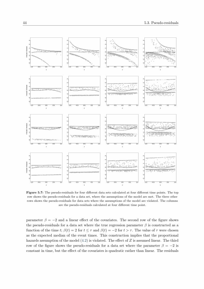
44 5.3. Pseudo-residuals
●●
●●
●
●●●●●●
●
●●
●
●●●●
●
●●●●
●
●●●●
●●
●●●●
●●
●●●●●●●
●●
●
●●
●●
●
●
●
●●
●●
●●●●●●
●
●
●
●●
●
●●
●●●
●●
●●●●●●●
●
●●●●●
●
●
●●●
●
●
●
●
●
●●
●●●
●●●
●
●
●
●
●
●
●
●●●●●●●
●
●
●
●●
●
●●●●●●
●
●●
●●●●●●
●●●
●
●
●
●
●●●
●●●●●●●●
●●
●●●●
●
●
●
●●●●●
●
●
●●●
●●●●
●
●
●
●●
●●
●●●●●
●●
●
●
●
●
●●●
●
●●●●●
●
●●●●●
●●
●●
●
●●●
●
●
●
●●
●●●
●●●
●●
●
●
●●
●
●●●●
●
●
●●●
●
●●●●●●
●
●●
●
●
●
●
●
●
●
●●●
●
●●●
●
●●●
●
●●●●●●●●●
●
●●●●
●
●●●●●●●●●●●●●
●
●●●
●●●
●●●●●
●
●
●●●
●
●●●
●
●●●
●
●●
●
●●●●●
●
●●
●
●●●●●●●●●●●●●●●●●●●
●
●●●●●●●●●●●●
●
●
●
●●●
●
●●●●●
●
●●
●
●
●
●●●
●
●●
●
●●●●●●
●
●●●●
●
●●●●●●●●●●
●
●●●
●
●●●●●●
●
●●●
●
●●●●●●●
●
●●●●●
●
●●●●
●
●●●●
●
●
●
●●●●●●●●●●●
●
●●●●●●●●●●●●●●●●●
●
●●
●
●●●●●●●●
●
●●●●●●●●●●●●●●●●●●●●
●
●●●●●●●●●●●●●
●
●
●●
●●●●●
●
●●●●●●●●●●●●●●●●●●●●
●
●●●●●●●●●●●●●●●●●
●
●●●●●●●●●●●●●
●
●●●●●●●●●●●
●
●●●●
●
●●●●●
●
●●●●●●●●●
●●
●●●●●●●●●
●
●●●●●●●●●●●●●●●●●●●●●●●●●●●●●●●●●●●●●●●●●
●
●●●●●●●●●●●●●
●
●●●●●●●●●●●●●●●●●●●●●●●●●●●●●●●●●●●●●●●●●●●●●●●●●
●
●●●●●●●
●
●●●●●●●●●●●●●●●●●●●●●●●●●●●●●●●●●●
●
●●●●●●●●●●●
●
●●●●●●●●●●●●●●●●●●●●●●●●●●●●●●●●●
●
●●●●●●●●●●●●●●●
●
●
●
●●●●●●●●●●●●
●
●●●●●●●●●●●●●●●●●●●●●●●●●●●●●●●●●●●●●●●●●●●●●●●●●●●●●●●●●●●●●●●●●●●●●●●●●●●●●●●●●●●●
●
●●●●●●●●●●●●●●●●●●●●
●
●●●●●●●●●●●●●
z
Pse
udo−
resi
dual
−3
−2
−1
01
23
−1.0 −0.5 0.0 0.5 1.0
●●●●
●
●●●●●●
●
●●
●
●●●●
●
●●●●
●
●●●●
●
●●●●●
●
●●●●●●●●
●●
●
●
●
●●
●
●●●●●
●
●●●●●●●●
●
●●
●
●●●●
●
●●
●●
●●
●●●●
●
●●
●
●
●
●
●●
●●
●
●
●
●
●●
●●●
●●
●
●●●
●
●
●
●
●
●
●
●
●●●
●
●
●
●
●
●●
●●
●
●
●
●
●●
●●●●●●●●●
●●●
●
●●●
●●●
●●●
●●
●●
●●●●
●●
●
●
●●
●●●
●
●●●
●●●●
●
●
●
●●●●
●●
●
●
●
●●
●
●
●
●
●●●
●●●●●●
●
●
●
●●
●●●
●
●●
●
●
●
●
●
●
●●
●●●
●●●
●●●●●
●
●●●
●
●
●
●
●
●●
●●
●
●
●●
●
●
●
●
●
●
●
●
●
●
●●●
●
●
●
●
●
●●
●●
●
●●●●●
●
●●●
●
●
●
●●
●●
●●●
●●
●●●
●●
●●
●
●●
●●●●
●
●
●●●
●
●●
●●
●
●
●●
●
●●●
●
●
●
●
●●●
●
●
●
●●
●
●●
●
●●●
●●
●
●
●●●●●
●●●
●
●
●
●●●●
●
●●●
●●●
●●●
●●●
●●●
●●●
●
●
●
●
●
●
●●●
●
●●
●
●●
●
●●●
●
●
●●●●●●●
●●●●
●
●●
●
●●●
●
●●
●
●●
●●
●●
●
●
●●●●
●
●●
●
●●●●●
●
●
●●
●
●
●●●●
●
●
●
●●●●●●
●
●
●
●
●
●●
●●●
●
●●●●
●
●●●●●●●
●
●
●●
●
●●●●●●●
●
●●●●
●
●●●●●●
●
●
●
●
●
●
●●●
●
●
●
●
●
●
●●●●●●●●
●
●
●●
●●
●
●●
●
●●●●●●●●●●●●●●●●●
●
●
●
●
●●●●●●●●●●●
●
●●●●
●
●
●●
●
●●●●●●●●●
●●
●●
●
●
●●●●●●
●●
●●●●
●
●●●●●
●
●●●●
●
●●●●
●●
●●●●●●●●●
●
●●●●●
●
●●
●
●●
●
●●●●●
●
●●●●●●●●●
●
●●●
●
●●●●●●●
●
●
●
●●●●●●
●
●●●●●●
●
●●●●
●
●●●●●●●●●●●●
●
●●●●●●●
●
●
●●●●●●●●●●●●●●●●●●●●●●
●
●●●
●
●●●
●
●●●●●●●●●●●●
●
●●●●●●
●
●
●●●●●
●
●●●●●●●
●
●●●●●●
●
●
●●●
●
●
●
●●●●●●●●●
●
●
●
●●●●●●
●
●●●●●●●●●●
●
●●
●
●●●●●●●●●●●●
●
●●
●
●
●
●●
●
●●●●●●
●
●●
●
●●
●
●●●
●
●●●●●●●●●
●
●
●
●●●
●
●
●
●
●
●
●
●●●
●
●●
●
●●●●●●●●
●
●
●
●●●●●●●●●●●
●
●●●●●●●●●●●●●●●●●●●●●
●
●●●
●
●●
●
●●●●●●●●●●●
●
●●●●●●●●
●
●●●●●●●●●●●●
z
−3
−2
−1
01
23
−1.0 −0.5 0.0 0.5 1.0
●●●●
●
●●●●●●
●
●●
●
●●
●
●
●
●●
●●
●
●●●
●
●
●
●●●
●
●
●
●
●
●●●●
●
●
●
●●
●
●●
●●
●
●
●●●●●●
●
●●●
●
●●●●
●
●●
●
●
●
●●●●
●●
●
●
●
●
●●
●
●
●
●
●
●
●
●●●
●●
●
●●
●
●
●
●
●
●
●
●
●
●
●
●
●
●
●
●
●
●●
●●
●
●
●
●
●
●
●●●●●●●●●
●●●
●
●●●
●
●
●
●●●
●
●
●●
●
●
●
●
●●
●
●
●●
●●●
●
●●●
●
●●
●
●
●
●
●●●●
●
●
●
●
●
●●
●
●
●
●
●●
●
●●●●●●
●
●
●
●
●
●●●
●
●●
●
●
●
●
●
●
●
●
●●●
●
●●
●●●●●
●
●●●
●
●
●
●
●
●●
●●
●
●
●●
●
●
●
●
●
●
●
●
●
●
●●●
●
●
●
●
●
●●
●
●
●
●
●●
●●
●
●●●
●
●
●
●●
●●
●●●
●●
●●●
●●
●
●
●
●
●
●●●●
●
●
●
●●
●
●●
●●
●
●
●
●
●
●
●●
●
●
●
●
●●
●
●
●
●
●
●
●
●
●
●
●
●●
●●
●
●●●●
●●
●●●
●
●
●
●
●
●
●
●
●●●
●●
●
●●●
●●
●
●●●
●●
●
●
●
●●
●
●
●
●
●
●●●
●
●
●
●
●●
●
●
●
●●●●●●●
●●●●
●
●
●
●
●●●
●
●
●
●
●
●
●●
●
●
●
●
●
●
●
●
●
●
●
●
●
●
●
●
●
●
●
●
●
●
●
●
●
●●
●
●
●
●●●●●
●
●
●
●
●
●
●●
●●
●
●
●
●
●●
●
●
●
●●
●●
●
●
●
●●
●
●●●●●
●●
●
●●●
●
●
●●
●
●
●●
●●
●
●
●
●
●●●
●
●
●
●
●
●
●●●●●●
●
●
●
●
●●
●●
●
●
●
●
●
●
●●
●
●●●●
●
●
●●●●●●
●
●
●
●
●●
●
●
●
●
●
●●●●
●
●●
●
●
●
●
●●
●
●●●
●
●●
●
●●
●●
●●
●
●
●●●
●
●
●
●●
●
●●
●
●
●
●●
●
●
●
●
●●
●
●
●●
●
●
●●
●
●
●
●
●●
●●
●
●
●●
●
●
●
●
●
●
●
●●
●
●
●
●
●●
●
●●
●
●●●
●
●●
●
●●●
●
●●●●●
●
●
●
●
●
●
●●●●●
●
●●●●●●
●
●●●●
●
●
●
●●●●●●
●
●
●
●
●
●●●●●●
●
●
●
●
●●
●●●●●
●
●
●
●
●
●●●
●
●
●
●
●●
●
●●
●
●
●
●
●
●
●●●●●●●●●●●●
●
●
●
●
●
●●
●
●
●●
●
●●
●
●●
●
●●
●
●
●
●
●
●
●
●●
●
●
●
●
●
●
●
●
●
●●●●
●
●●●
●
●
●
●
●
●
●
●●
●
●●●●●●●●●●
●
●●
●
●●●●●●●●●●●
●
●
●●
●
●
●
●
●
●
●
●
●●●●
●
●
●
●
●●
●
●●●
●
●●●●●●●●●
●
●
●
●●●
●
●
●
●
●
●
●
●
●●
●
●●
●
●●●●●●
●
●
●
●
●
●●●●●●●●●●
●
●
●
●●●●●●●●
●
●●●●●●●
●
●●●
●
●
●●
●
●●
●
●●●●●●
●
●●●●
●
●●●●●
●●
●
●
●●●●
●
●
●●●●
●
●
●
z
−3
−2
−1
01
23
−1.0 −0.5 0.0 0.5 1.0
●
●
●
●
●
●
●
●
●
●
●
●
●●
●
●
●●●
●
●
●
●
●●
●
●
●
●
●●
●
●
●
●
●
●●
●
●
●
●
●
●
●
●
●●
●
●
●●
●
●
●
●
●
●●●
●
●
●
●●
●
●●
●
●
●
●
●●
●
●
●
●
●
●
●
●
●
●
●
●
●
●
●
●
●
●
●
●
●
●
●
●
●
●
●
●
●
●
●
●
●
●
●
●
●
●●
●
●
●
●
●
●●●●
●
●
●●
●
●
●
●
●
●
●●
●
●
●
●●
●
●
●●
●
●
●
●
●
●
●
●
●
●
●
●
●●●
●
●
●
●
●
●
●
●●
●
●
●
●
●
●
●
●
●●
●
●
●
●
●
●
●●●
●●
●
●
●
●
●
●
●●
●
●●
●
●
●
●
●
●
●
●
●●●
●
●●
●●●●
●
●
●●●
●
●
●
●
●
●
●
●●
●
●
●●
●
●
●
●
●
●
●
●
●
●
●
●●
●
●
●
●
●
●●
●
●
●
●
●●
●
●
●
●●●
●
●
●
●
●
●●
●●●
●●
●
●
●
●●
●
●
●
●
●
●●●●
●
●
●
●
●
●
●●
●
●
●
●
●
●
●
●
●●
●
●
●
●
●●
●
●
●
●
●
●
●
●
●
●
●
●●
●●
●
●●●●
●
●
●●●
●
●
●
●
●
●
●
●
●●●
●●
●
●●●
●
●
●
●●●
●
●
●
●
●
●●
●
●
●
●
●
●●●
●
●
●●
●●
●
●
●
●●●●●●●
●●
●
●
●
●
●
●
●
●●
●●
●
●
●
●
●●
●
●
●●
●
●
●
●
●
●
●
●
●
●
●
●
●
●●
●
●
●●
●
●
●
●
●
●
●
●
●●●●
●
●
●
●
●
●
●●
●
●
●
●
●
●
●●
●●
●
●
●
●●
●
●
●
●●
●
●
●●
●●
●●
●
●
●
●
●
●
●
●
●
●●
●
●●
●
●
●
●
●●
●
●
●
●
●
●
●
●●●
●
●●
●
●
●
●
●●
●●
●
●
●
●
●●
●●
●
●●
●
●
●
●
●
●
●
●
●
●
●
●
●●
●
●
●
●
●
●
●
●
●
●
●
●
●
●
●
●
●
●
●
●
●
●
●
●
●
●●
●
●●
●●
●
●
●
●
●
●
●
●
●
●
●●
●
●
●
●
●
●
●
●
●
●
●
●
●●
●●
●
●
●
●
●●
●
●
●
●
●
●
●●
●
●
●●
●
●
●
●
●
●
●
●
●
●
●
●
●
●
●
●
●
●
●
●●●
●
●●
●
●●●
●
●
●
●
●●
●
●
●
●
●
●
●●
●
●
●
●
●
●●●●
●
●
●
●●
●
●
●
●
●
●●●●
●
●
●
●
●
●
●
●
●
●●
●
●
●
●
●
●●
●
●
●
●
●
●
●
●
●
●
●
●
●
●●
●
●
●
●
●
●
●
●
●
●
●
●
●
●
●
●
●
●
●●
●
●●●
●
●●
●
●●
●
●
●
●
●●
●
●
●
●
●
●
●
●
●
●
●
●
●
●
●
●
●●
●
●
●
●
●
●
●
●
●
●
●
●●
●
●
●●
●
●
●
●
●
●
●
●
●
●
●
●
●●
●
●
●
●
●
●
●
●●
●
●●●
●
●
●●●●
●
●
●
●
●
●
●
●
●
●
●
●
●
●
●●●●
●
●
●
●
●●
●
●●●
●
●
●
●
●
●
●●
●
●
●
●
●
●●●
●
●
●
●
●
●
●
●
●●
●
●
●
●
●
●
●●●●
●
●
●
●
●
●●
●
●
●●●
●
●●
●
●●
●●●
●
●●
●
●
●
●
●●
●●●●
●
●●●
●
●
●●
●
●
●
●
●
●●
●
●●
●
●
●
●
●
●
●
●
●
●
●
●●
●
●
●●●●
●
●
●●●●
●
●
●
z
−3
−2
−1
01
23
−1.0 −0.5 0.0 0.5 1.0
●●
●●
●
●
●●●●●
●
●●
●
●
●
●
●●●●
●
●●●
●
●●●●●●●●
●
●●●●●●
●
●●
●
●●
●●●
●●●●●●●
●
●●●●●●●●●●●●●●●
●
●
●●●●●
●
●●●●
●
●
●
●●●●●●●
●●
●●●
●
●●●
●
●●
●
●
●
●
●
●
●●
●
●
●
●●●
●
●
●
●●●●●●●●●●●●●●●●●●●●●●●●●
●
●●●●●●
●
●
●●
●
●●●●●
●
●
●
●●●●
●
●
●
●
●
●
●●●●●
●
●●
●●
●●●
●
●●●●●
●
●●●
●
●
●
●●●
●
●●●●●
●
●●●●●●●
●
●●
●
●●●
●
●
●
●●
●
●●
●●●●●
●
●
●
●
●
●
●●●●●
●●
●●●●●
●
●●●●●●●●
●
●●
●
●●●●●●
●
●●●●●
●
●●●●●●●●●
●●
●
●
●●
●
●
●●
●
●●●●●●●●●
●
●
●
●●●●
●●
●
●
●●●
●
●
●
●●
●
●●●●●●●
●
●●
●
●●●●●●●●●
●
●●●●
●
●●●
●
●●●●
●
●
●●●●●●●
●
●●
●●
●●
●●
●●●
●●
●●●
●
●●
●
●●●●●●●●●●●●●●●●●●●●●●●●●●●●●●●
●
●●●
●
●
●
●
●
●
●
●●●
●
●●●●●●●●●●
●
●●●●●●●●●●●●●●●●●●●●●
●
●●●●●●●●
●
●●●●●●●●
●
●●●●●
●
●
●●●●
●
●●●●●
●
●
●
●
●●
●●
●●
●
●●●●●●●●●●●●●●●
●●
●●●●●●
●
●●●●
●
●●●●●●●●●●●●
●
●
●
●●
●
●●●●●●●●●
●
●
●
●
●●●●●●●●●●●●●
●
●●●●●
●
●●●●●●●●●
●
●●
●
●●●●●●●●●●●●●●●●●
●
●
●
●●●●●●●●●●●
●
●●●●●●●●●●●●●
●
●●●●●●●●●●●●
●
●●●●●●●
●
●●●●●
●●
●
●●
●●●●
●
●
●
●●●●●●●
●
●●●●●●●●●●●●●●●●●●●
●●
●
●●
●
●
●●●●●●●
●
●●●●
●
●●●●●
●
●●●
●●
●●
●
●●●●●●●
●
●●●●●
●
●
●
●
●●●●●●●●●●●●●●●●●●
●
●●●●
●
●●●
●
●●●●●●
●
●●●●
●
●
●●●●
●●●●
●
●●●
●
●●●●●
●
●●
●●
●●●●●●●●●●
●
●
●
●●
●●
●
●
●●
●●
●
●●●
●●
●
●
●●
●●●
●
●
●●●●
●●
●●●
●
●●
●●●●
●●●●
●
●●
●
●
●●●●
●
●
●●
●●●
●
●●●
●●
●●
●
●●●
●
●●●●
●●
●●●
●●
●
●
●●●●●●●●
●
●●
●●
●
●
●●●
●●
●●
●
●●●
●
●●●
●
●●
●
●
●●
●●●●●●
●
●●●
●●
●●
●
●●●●
z
Pse
udo−
resi
dual
−3
−2
−1
01
23
−1.0 −0.5 0.0 0.5 1.0
●
●
●●
●
●
●
●
●
●
●
●
●●
●
●
●
●
●●●
●
●
●●●
●
●●●●
●
●●●
●
●●●
●
●
●
●
●
●
●
●●
●●●
●●●●●●●
●
●●●●●●●●●●
●
●
●
●
●
●
●
●
●
●●●
●●
●
●●●
●
●
●
●●●
●
●
●●●
●●●
●●
●●
●
●
●
●
●
●
●
●
●
●
●●
●
●
●
●
●
●●●
●
●●
●●
●
●●●●●●●
●●
●
●
●●
●
●
●
●●●
●●
●●●●
●●
●
●
●
●
●●
●●●●
●
●●●●
●
●●●
●
●
●
●●
●
●●
●
●
●
●●●●●●
●
●●●●
●
●
●
●
●●●
●
●
●
●
●●●●●
●●●
●●●●●
●
●
●
●
●
●●
●●
●
●●
●
●●
●
●●●
●●
●
●
●
●
●
●
●
●●●
●●●
●
●
●
●●
●●●
●
●
●
●●
●
●
●●
●●●
●
●●
●●
●●●●
●
●●●●●
●
●●
●●●
●
●
●
●
●
●
●●
●●
●●
●
●
●
●●●
●
●
●
●●●
●●●
●
●
●
●
●
●●
●
●●
●
●
●
●●●
●
●
●
●●
●
●●
●●
●
●●●
●
●
●●
●
●
●
●●●
●
●
●●●●
●
●●●●●●
●●
●●
●●
●●
●●
●●
●●●
●
●
●
●
●●
●
●●●●
●
●●●
●
●●●●
●
●●●
●
●
●
●
●●
●●
●●●
●
●●●
●●●
●
●
●
●
●
●
●
●●●
●
●●●●●
●
●
●●●
●
●
●●●●
●
●●●●●●●●●
●
●
●●
●
●
●
●
●●
●
●
●●
●
●
●
●
●●●●●●
●●●
●●
●●
●
●●●●
●
●●●●
●
●
●
●
●
●●
●●
●●
●
●
●●
●●●●●
●
●●●●
●●●●
●●●●
●
●
●
●
●●●
●
●
●●●
●
●●●●●●
●●●
●
●●
●
●●●●●●●●●
●
●
●
●
●
●
●●●●●●●●●
●
●
●
●
●
●
●●
●
●●●●●
●
●●●
●
●●
●
●●
●●
●●●●●●●
●
●
●
●●●
●
●
●
●
●
●●●●●
●
●●
●
●
●●●●●●
●
●●●●●
●
●
●●●●
●
●●
●
●●
●●
●
●
●
●●●
●●
●●
●
●
●●
●●
●
●●
●●
●●
●
●
●●
●●
●●
●●
●
●
●
●●●●●●●
●●
●●●●●●
●
●
●●
●
●●
●
●
●●●
●●
●●
●
●●●●
●
●●●●
●●
●●
●●●
●●
●●●
●●●●
●
●
●●●●●
●●
●
●
●●
●
●
●
●
●
●
●
●●
●
●●●●
●
●
●
●
●
●●
●
●●●
●●
●
●●
●
●●
●
●
●●
●
●
●●●●
●●●●
●
●●●
●●
●●●●
●
●
●
●●
●●●●●●●●●
●
●
●
●
●●
●
●
●
●
●●
●
●
●
●
●
●
●●
●
●
●
●
●●●
●
●
●
●●
●
●●
●●●
●
●●
●●●●
●
●
●●
●
●●
●
●
●●●
●●
●
●●
●●●
●●
●●
●●
●
●●
●●●
●●
●●●
●●
●●
●●●
●
●
●●●●●●●●
●●
●
●●
●
●
●
●
●●●
●●
●
●
●
●
●
●●
●
●
●
●●
●
●●
●
●●
●●●
●●●●
●●●
●
●
●●
●
●
z
−3
−2
−1
01
23
−1.0 −0.5 0.0 0.5 1.0
●
●
●●
●
●
●
●
●
●
●
●
●●
●
●
●
●
●●
●●
●
●●●
●
●
●
●
●
●
●●
●
●
●
●
●●
●
●
●
●
●
●
●
●
●●●
●
●●●
●
●●
●
●●●●
●
●
●
●●
●
●
●
●
●
●
●
●
●
●
●
●●
●●
●
●●●
●
●●
●●
●●
●
●●●
●
●
●
●●
●
●●●●
●
●●●
●
●
●
●●
●
●
●
●
●
●●●
●
●●
●
●●
●
●
●●●
●
●
●●
●
●●
●
●
●
●●
●
●
●●
●
●
●
●
●●
●
●●●
●●
●●●●
●
●●●●
●
●●●
●
●
●●
●
●
●●
●
●
●●●●●●●
●
●
●
●●
●●
●
●
●●●
●
●
●
●
●●●
●
●
●●●
●●
●
●●
●
●
●
●
●●●
●●
●
●●
●
●●
●
●
●
●●●
●
●
●
●
●
●
●
●●●
●●●
●
●●●●●
●
●
●
●
●
●
●
●
●
●●
●
●
●
●
●
●
●●●●●
●
●
●●●
●
●
●
●
●●●●
●
●
●●
●
●●
●
●●
●
●●
●
●
●
●
●
●
●
●
●
●●
●●●
●
●
●
●
●
●●●
●
●
●
●
●●
●
●
●
●
●
●
●
●
●●
●
●●
●
●
●
●
●
●
●
●
●
●
●
●●
●
●
●●●●
●
●
●
●●
●●●●
●
●
●●
●●
●●
●
●●●●●
●
●
●
●
●
●●●
●
●
●
●●●
●
●
●
●
●●
●●
●
●
●
●
●
●●
●
●
●●●
●
●●●●
●
●●
●
●●
●
●
●
●
●
●
●
●
●
●
●●
●
●●
●
●
●
●
●
●
●●●
●
●
●
●
●
●
●
●
●
●
●
●
●●●●
●
●●
●
●●●
●
●
●
●
●●
●
●
●
●
●●●
●
●●●
●
●
●●
●●
●
●●
●
●
●
●
●
●
●●●●
●●●
●
●●
●
●●
●
●
●
●
●
●
●
●●●●
●
●
●●
●
●
●
●
●
●
●
●
●
●●●
●
●●
●●●
●
●●●●
●●
●
●
●●●
●●●
●
●
●
●
●
●
●
●
●
●
●
●●
●
●
●
●
●●●
●
●
●●
●
●
●●●
●
●
●
●
●
●
●
●●
●●
●
●●
●
●
●
●●
●
●
●●●
●
●
●
●
●
●
●
●
●●●
●
●●
●
●●
●
●
●
●
●●
●
●●●●
●●
●
●
●
●
●●
●
●
●
●
●
●
●●●●●
●
●●
●●●●
●
●●●
●●
●
●●
●
●
●●●
●
●●●●
●●
●
●
●●
●
●
●
●
●
●●
●
●●
●●
●
●●●
●
●
●●
●
●●
●
●
●
●
●
●●
●●
●
●
●
●●
●
●
●●
●●●
●
●
●●●
●●
●●●
●
●
●●
●
●
●●●●
●
●●
●
●
●●
●
●
●
●
●
●
●
●
●
●
●
●
●
●
●
●
●
●
●●
●
●
●
●
●
●●●
●●
●●●
●
●
●
●
●●●●●●
●
●●
●
●
●
●
●
●●
●
●
●●
●
●
●
●●
●
●
●●●
●
●
●
●
●
●
●
●
●●
●
●
●
●
●●
●
●●
●
●
●
●●
●
●●
●
●●●
●
●
●
●●
●
●●
●●
●
●
●
●
●●●●
●
●
●●
●
●
●
●
●
●●●
●●
●
●●
●
●
●
●●
●●
●●
●
●●
●
●
●
●●
●
●
●
●●●●●●●
●
●
●●
●●
●●●●
●●
●
●●
●
●
●
●
●●●
●●
●
●
●●
●
●●
●●●●●
●
●●
●
●●
●●
●
●●●●●●●
●
●
●
●
●
●
z
−3
−2
−1
01
23
−1.0 −0.5 0.0 0.5 1.0
●
●
●●
●
●
●
●
●
●
●
●
●
●
●
●
●
●
●●
●●
●
●●
●
●
●
●
●
●
●
●
●
●
●
●
●
●●
●
●
●
●
●
●
●
●
●●●●
●●●
●
●
●
●
●●●
●
●
●
●
●●
●
●
●
●
●
●
●
●
●
●
●
●
●
●●
●
●●●
●
●●
●●
●●
●
●●●
●
●
●
●●
●
●●●●
●
●●●
●
●
●
●●
●
●
●
●
●
●●●
●
●●
●
●●
●
●
●●●
●
●
●●
●
●●
●
●
●
●●
●
●
●●
●
●
●
●
●●
●
●●●
●
●
●●●●
●
●●●●
●
●●●
●
●
●●
●
●
●
●
●
●
●●●●●●●
●
●
●
●●
●●
●
●
●●●
●
●
●
●
●●
●
●
●
●●●
●
●
●
●
●
●
●
●
●
●●●●●
●
●●
●
●●
●
●
●
●●●
●
●
●
●
●
●
●
●●●
●●●
●
●●●●●
●
●
●
●
●●
●
●
●
●●
●
●
●
●
●
●
●●●●●
●
●
●
●
●
●
●
●
●●●●●
●
●●●
●
●●
●
●●
●
●●
●
●
●
●
●
●
●
●
●
●
●
●●●
●
●
●
●
●
●●●
●
●
●
●
●●
●
●
●
●
●
●
●
●
●●
●
●●
●
●
●
●
●
●
●
●
●
●
●
●●●
●
●●●●
●
●
●
●
●
●●●●
●
●
●●
●●
●●
●
●●●●●
●
●
●
●
●
●●●●●
●
●
●
●
●
●
●
●
●●
●●
●
●
●
●
●
●●
●
●
●●●
●
●●●●
●
●●
●
●●●●●
●
●
●●
●
●
●
●●
●
●●
●
●
●
●
●●
●●●●
●
●
●
●●
●
●
●
●
●
●
●●●●
●
●●
●
●●●
●
●
●
●
●
●
●
●
●
●
●●●
●
●●●
●
●
●●
●●●
●●
●
●
●
●●
●
●●●●●●●
●
●●
●
●●
●
●
●
●
●
●
●
●●●●
●
●
●●
●
●
●
●
●
●
●●
●
●●●
●
●●
●●●
●●●●●
●
●
●
●
●●●
●●●
●
●●
●
●
●
●
●
●
●
●
●●
●
●
●
●
●●●
●
●
●●
●
●●●●
●
●
●
●
●
●
●
●●●●
●
●●
●
●
●
●●●
●
●●●
●
●
●
●●●
●
●
●●●
●
●●
●
●●
●
●●
●
●●
●
●●●●
●
●
●
●
●
●
●●
●
●
●
●
●
●
●●●●●
●
●●
●●●●
●
●●●
●●
●
●●
●
●
●●●
●
●●●●●●
●
●
●●
●
●
●
●
●
●
●
●
●●
●
●
●
●●●
●
●
●●●●●
●
●
●
●
●
●●●●●
●
●
●●
●
●
●●
●●●
●
●
●●●
●●
●●●
●
●
●●
●
●
●
●
●●
●
●●
●
●
●●
●
●
●
●
●
●
●
●
●
●
●
●
●
●
●
●
●
●
●●
●
●
●
●
●
●●●
●●
●●●
●●
●
●●●●●●●
●
●●
●
●
●
●
●
●●
●
●
●●
●
●
●●●
●
●
●●●
●
●
●
●
●
●
●
●
●●
●
●
●
●●●
●
●●
●
●
●
●●
●
●●
●
●●●
●
●
●
●●
●
●●
●●
●●
●
●
●●●●
●
●
●
●
●
●
●
●
●
●●●
●●
●
●●
●
●
●
●●
●●
●●
●
●●
●
●
●
●●
●
●
●
●●●●●●●
●
●
●
●
●●
●●●●
●●
●
●●
●
●
●
●
●●●
●
●
●
●
●●●
●
●
●●●●●
●
●●
●
●●
●●
●
●●●●●●●
●
●
●
●
●
●
z
−3
−2
−1
01
23
−1.0 −0.5 0.0 0.5 1.0
●●●●●●●●●●●●●●●●●●●●●●●
●
●●●
●
●●●●●●●●●●●●●●●
●
●●●●●●
●
●●●●
●
●●
●
●●●●●●●●●●●●●●●●●●●●
●
●●●●●●●●●●●●●●●
●
●
●●●●●●●●●●●●●●
●
●●●●●●●●
●
●●
●
●
●
●
●●
●
●●●●●●●●●●
●
●
●
●●●●●●●●●●●●
●
●
●●●●●●
●
●●●
●
●●●●
●
●
●
●●
●
●
●●
●
●●
●●
●
●
●●●●
●
●
●●●
●
●●
●
●●●
●
●●●●●●●●●
●
●●●●●●●●●●●
●
●●●●
●
●●●
●
●
●●●●●●●●●
●
●●●●●●●●●●●
●
●
●
●●
●
●●●
●
●●●●
●
●●
●
●●●●
●●
●●
●
●●●●●
●
●●●
●
●
●
●
●
●●
●
●●●●●●●●●
●
●●●
●
●●
●
●
●
●●●
●
●●●
●
●●
●●●●●●●●
●
●●●●●●●●●
●
●●●
●
●
●
●●●●●●
●
●●●●●●
●
●●
●
●
●●●
●
●●●●●●●●●●●●
●
●●
●
●
●
●●●●●●●●●
●
●●●●●●●
●
●●●●●●●●●●●
●
●
●
●●●●
●●
●●●●●●●
●
●●●●
●
●●●●●●●●●●●●●●●●●●●●●●●
●
●
●●●●●●
●
●
●●●●
●
●
●
●●●●●●●●●●●●●●●●●
●
●●●●●●●
●
●●●●
●
●●●●●●
●
●
●
●●●
●●
●●●●
●●
●●
●
●●●●●●●●●●
●
●
●●
●
●●●
●
●
●
●●●
●
●●●
●●
●
●●
●●●●
●
●●●
●
●●●
●
●
●●
●
●
●●●●●●●●●●●●●●●●●●
●
●●
●●●●●●●●
●●
●●●
●●
●
●
●●●
●
●
●
●●●●●●●●●●●●●
●
●
●
●
●
●●●●●
●
●●●●●●●●
●
●
●
●●●●●
●
●●●●●●●●●
●
●●●●●
●
●●●●●●●
●
●
●
●●●●
●
●
●
●
●●●●●●
●
●●●●●●●●●●●●●
●
●
●
●●●●●●●
●
●
●
●●●●●●●
●
●●●●●●●●
●
●●●●●
●
●●
●
●●●●●
●
●●●●●●●●●●●●●●●●●●●●●●●●
●
●●
●
●
●●●●●●
●
●
●
●●
●
●●●●●
●
●●●●●●●●●
●
●●●●●●●●●
●
●●●●●●●●●●●●●●●●●●●
●
●●●●
●
●●●●●●●●●●●●●●●●●●●
●
●●●●●●●●●●●●●●●●●●●●●●●
●
●●●●●●●●●●●●●●●●●
●
●●●●●
●
●
●●●●●●●●●
●
●●●●●●●●●●●●●●●●●●●●●●●●
●
●●●●●●●●●●●●●●●●●●●●●●●●●●●●
z
Pse
udo−
resi
dual
−3
−2
−1
01
23
−1.0 −0.5 0.0 0.5 1.0
●●●●
●
●●●●●●
●
●●●●●●●●
●
●●
●
●
●
●
●
●●
●
●●●●●●●●●●●●
●
●●●●●●
●
●●
●
●
●
●●
●
●●
●
●●●●●●●
●●
●
●
●
●●●●●
●
●
●
●●●●●●
●
●
●●●●●
●●
●
●
●
●
●
●
●●●●●●
●
●
●
●●
●
●
●
●●●
●
●●
●
●
●
●
●
●
●
●●●●●●
●
●
●●
●
●
●
●●●●●
●
●●●●●
●
●
●
●●●●●●
●
●
●
●
●
●
●
●
●
●
●
●
●●
●
●
●
●
●
●●
●●
●
●
●
●
●●
●
●
●●●
●
●
●
●
●●●
●
●
●
●●●●●●●
●
●●
●
●
●●
●
●●●
●
●
●●●●
●
●
●●
●●
●●●●●●●●●
●
●
●●●●
●
●●●●●
●
●
●
●●
●
●●●
●
●
●
●●
●
●●
●
●●
●
●
●●
●
●
●
●●●
●
●
●
●●
●●
●
●
●
●
●
●
●
●
●●
●
●
●●
●
●
●
●●●
●
●
●
●●
●
●
●
●
●
●●●
●
●●
●
●●●●
●
●●
●
●
●
●
●●
●
●
●●
●
●●●
●
●
●
●●●
●
●●
●
●
●
●●●●
●
●
●
●●
●●●
●
●●●●●●
●●
●
●
●
●
●
●●
●
●
●
●
●●
●
●
●
●
●●
●
●●●●
●
●●
●
●●●●
●
●
●
●●●
●
●
●
●●
●
●
●
●●
●●
●
●
●
●
●
●
●
●
●
●
●
●
●
●●●●●●
●
●●
●
●
●
●
●
●●
●●●
●
●
●
●
●●
●●●●
●
●
●
●
●●
●
●
●
●
●
●
●●
●
●●●
●
●
●
●●●●
●
●
●
●
●
●
●●●
●
●●
●
●
●
●
●
●●
●
●
●
●
●
●●●
●●
●
●●
●
●●
●
●
●
●●●●
●
●●●
●
●
●
●
●●
●
●●
●
●
●
●
●●●
●
●
●
●
●●
●
●●
●
●
●
●
●
●
●
●
●
●●
●
●
●
●
●
●
●
●●●●●●
●
●●●●●
●
●●●
●●
●
●●
●●●
●●●
●
●
●●
●●●
●●
●
●
●●
●
●
●
●
●●
●
●●●
●
●●●●●
●
●
●
●●●
●●●●●
●
●
●
●
●●●●●
●
●
●
●
●●●
●
●
●●●
●
●●●●●
●
●
●●●
●
●
●●
●
●
●
●
●
●
●
●
●
●
●
●
●
●
●
●
●
●●
●●
●
●
●
●
●●●●●●
●
●●●●
●
●
●
●
●
●●●●●
●
●
●
●●
●
●●●●
●
●
●
●●●
●
●●
●
●●●
●
●
●
●
●
●
●●
●
●
●
●
●●
●
●●●●●●●●
●
●●
●
●●
●
●
●
●●●●
●
●●
●
●
●●
●●
●●
●
●
●
●●
●
●●
●
●
●
●
●●●●●●
●
●●
●
●●
●
●
●
●●●●
●
●
●●●●●●●●
●
●●●●●●●
●
●
●
●●
●
●
●
●●●●●●●●
●
●●●●●
●
●●●●
●
●
●●●●●●
●
●●●
●
●●●
●
●●●●●●●
●
●●●●●●●●●●●●
●
●
●
●●
●
●●●●●
●●
●●●●●●●●●
●
●●●
●
●●●●●●●●●●●
●
●●●●●●●●
●
●●●
●
●●●●●●●●●●
●
●
●
●●
●
●●
●
●●●●●
z
−3
−2
−1
01
23
−1.0 −0.5 0.0 0.5 1.0
●
●
●●
●
●
●●●
●
●
●
●●
●
●●
●
●●
●
●●
●
●
●
●
●
●
●
●
●●●●●
●
●●●●●●
●
●●
●
●●●
●
●●
●
●
●
●
●
●
●
●
●
●
●●●●●●
●●
●
●
●
●●
●
●●
●
●
●
●●●●●
●
●
●
●●●●●
●●
●
●
●
●
●
●
●●●
●
●●
●
●
●
●
●
●
●
●
●●●
●
●
●
●
●
●
●
●
●
●
●●
●●
●●
●
●
●
●
●
●
●
●●●●●
●
●
●●●●
●
●
●
●●●●
●
●
●
●
●
●
●
●
●
●
●
●
●
●
●●
●
●
●●●
●
●
●●
●
●
●
●
●
●
●
●
●●●
●
●
●
●
●
●
●
●
●
●
●●●●●●
●
●
●
●
●
●
●
●●
●
●
●
●
●
●
●
●
●
●
●
●●
●●
●●
●
●
●
●
●●●
●
●
●●●●
●
●
●
●
●
●
●
●
●
●
●
●
●●
●
●
●
●
●
●
●
●
●
●
●●
●
●
●●
●
●
●
●
●●
●
●
●
●
●
●●
●
●●●
●
●
●
●
●
●
●
●
●●
●
●
●
●●
●
●
●
●
●●
●
●
●
●
●
●
●
●
●
●●
●
●
●●
●
●
●●
●
●
●
●
●
●
●●
●
●
●
●●
●
●
●
●
●
●
●
●
●
●
●
●
●
●●●
●
●
●
●
●●
●●
●
●
●●●●
●●
●●
●
●
●
●
●
●●
●
●
●
●
●
●
●
●
●
●
●●
●
●
●●
●
●
●
●
●
●
●
●
●
●
●
●
●
●
●
●
●
●
●●
●
●
●
●●
●
●
●
●
●
●●
●
●
●
●
●
●
●
●
●
●
●●
●
●
●
●
●
●
●
●●
●
●●●●●
●
●
●
●●●
●
●
●
●
●●
●
●
●●
●
●
●
●
●
●
●
●
●
●●●
●
●
●
●●●●
●
●
●
●
●
●
●●●
●
●
●●
●
●
●
●
●
●
●
●
●
●
●
●●●
●●
●
●
●
●
●●
●
●●
●
●
●
●
●
●●●
●
●
●
●
●●
●
●
●
●
●
●●
●
●
●
●
●
●
●
●●
●
●●
●
●
●
●
●
●
●
●
●
●●
●
●●
●
●
●
●
●●
●
●●●
●
●
●●
●
●
●
●●●
●●
●
●●
●●●
●
●
●
●
●
●●
●●●
●●
●
●
●●
●
●
●
●
●
●
●
●
●
●
●
●●●●●
●
●
●
●●●
●
●
●
●
●
●
●
●
●
●
●●
●
●
●
●
●
●
●●●
●
●
●●●
●
●
●●
●
●
●
●
●
●●
●
●
●
●
●
●
●
●
●
●
●
●
●
●
●
●
●
●●
●
●
●●
●
●
●
●
●
●
●
●●
●
●
●
●
●
●
●●
●
●
●
●
●●
●
●●●
●
●
●
●
●
●
●
●●●
●
●
●
●●
●
●
●●
●
●●●
●
●
●
●●
●
●●
●
●
●
●
●●
●
●
●
●
●
●●
●
●
●
●
●
●
●●
●
●
●
●●●
●
●
●●
●
●
●
●
●●
●●
●
●
●
●
●
●
●
●
●●
●
●
●
●●●
●
●
●
●
●
●
●
●
●
●
●
●
●
●
●
●
●
●
●●●●
●
●●
●
●●●●●
●
●
●
●
●
●●
●
●●
●●●●
●
●●●
●
●
●
●●●
●
●
●
●●
●
●
●
●
●
●●●
●
●●●
●
●●●
●
●
●
●
●
●
●●
●
●●●●
●
●
●
●●●●●
●
●
●
●
●
●
●
●●
●●
●●
●
●
●●●●
●
●
●
●
●●●
●
●
●●●
●●●
●
●
●●
●
●●
●
●
●
●●●
●
●●
●
●
●
●●●●●
●
●●●
●
●
●
●●
●
●●
●
●
●
●
●●
z
−3
−2
−1
01
23
−1.0 −0.5 0.0 0.5 1.0
●
●
●●
●
●
●●●
●
●
●
●●
●
●●
●
●●
●
●
●
●
●
●
●
●
●
●
●
●●●●
●
●
●●●
●●
●
●
●
●
●
●●●
●
●
●
●●
●
●
●
●
●
●
●
●
●
●
●
●
●●
●●
●
●
●
●●
●
●●
●
●
●
●●●●
●
●
●
●
●
●
●
●
●
●●
●●
●
●
●●
●
●
●
●
●
●
●
●
●
●
●
●
●
●
●●●
●
●
●
●
●
●
●
●
●
●
●
●
●●
●●
●
●
●
●
●
●
●
●●
●
●
●
●
●
●
●
●●
●●
●
●●●●
●
●
●
●
●
●
●
●
●
●
●
●
●
●
●
●
●
●
●●●
●
●
●●
●
●
●
●
●
●
●
●
●
●
●
●
●
●
●
●
●
●
●
●
●
●
●
●
●
●
●
●
●
●
●
●●
●
●●
●
●
●
●
●
●
●
●
●
●
●
●
●
●●
●
●
●
●
●
●
●
●
●
●
●
●●
●
●
●
●
●
●
●
●
●
●
●
●
●
●
●
●
●
●
●
●
●●
●
●
●
●
●●
●
●
●●
●
●●
●
●
●
●
●
●
●
●
●●
●
●●●
●
●
●
●
●
●
●
●
●●●
●
●
●
●
●
●
●
●
●●
●
●
●
●
●
●
●
●
●
●●
●
●
●
●
●
●
●
●
●
●
●
●
●
●
●●
●
●
●
●
●
●
●
●
●
●
●
●
●
●
●
●
●
●
●●●●
●
●
●
●●
●
●
●
●
●●
●●
●●
●
●
●
●
●
●
●
●
●
●
●
●
●
●
●
●
●
●
●
●●●
●
●
●●
●
●
●
●
●
●
●
●
●
●
●●
●
●
●
●
●
●●
●●
●
●●
●
●
●
●
●
●●
●
●
●
●
●
●
●
●
●
●
●
●
●
●
●
●
●
●
●
●●
●
●●●●●
●
●●
●●●
●
●
●
●
●●
●
●
●●
●
●
●
●
●
●
●
●
●
●●
●
●
●
●
●
●
●●
●
●
●
●
●
●
●
●
●
●
●
●●
●
●
●
●
●
●
●
●
●
●
●
●
●
●
●●
●
●
●
●●●
●
●●
●
●
●
●
●
●●●
●
●
●
●
●●
●
●
●
●
●●●
●
●
●
●
●
●
●
●●
●
●●
●
●
●
●
●
●
●
●
●
●
●
●
●●
●
●
●
●
●
●
●
●●
●
●
●
●●
●
●
●●●●
●
●
●
●●
●●●
●
●
●
●
●
●●
●
●
●
●●
●
●
●●
●
●
●
●
●
●
●●
●
●
●
●●●●
●
●
●●●●●
●
●
●
●
●
●
●
●●
●
●
●
●
●
●
●
●
●
●●●
●
●
●
●
●
●
●
●
●
●
●
●
●
●
●
●
●●
●
●
●
●
●
●
●
●
●
●
●
●
●
●
●
●●
●
●
●●
●
●
●
●
●
●
●
●
●
●
●
●
●
●
●
●
●
●
●
●●
●●
●
●
●
●
●
●
●
●
●
●
●
●
●
●
●
●
●
●
●
●
●
●
●
●
●●●
●
●
●
●●
●
●
●
●
●
●
●
●
●
●
●
●
●
●
●
●
●
●
●
●
●
●
●●
●
●
●
●
●
●
●
●
●●
●
●
●
●
●●
●●
●
●
●
●
●
●
●
●
●●
●
●
●
●●●
●
●
●
●
●
●
●
●
●
●
●
●
●
●
●
●
●
●
●●
●
●
●
●
●
●
●
●●
●
●
●
●
●
●
●
●
●
●
●●
●
●●●
●
●
●
●
●
●
●
●
●
●
●
●
●
●
●
●
●
●
●
●
●●●
●
●
●●
●
●●●
●
●
●
●
●
●
●●
●
●●●●
●
●
●
●
●
●●●
●
●
●
●
●
●
●
●●
●●
●●
●
●
●●
●
●
●
●
●
●
●●●
●
●
●
●
●
●●●
●
●
●●
●
●
●
●
●
●
●
●
●
●
●●
●
●
●
●
●
●●
●
●
●●
●
●
●
●
●
●
●
●●
●
●
●
●
●●
z
−3
−2
−1
01
23
−1.0 −0.5 0.0 0.5 1.0
●●
●●●
●●
●
●
●
●●
●
●
●
●●●●●●●●●
●
●
●
●
●●●●●●●●
●
●●
●●
●
●●●●●●●●
●
●●
●●
●●●●●
●●
●●●●●●●
●●
●●●●
●●
●
●
●
●
●
●●
●●●●●
●
●
●●●
●●●●●●●
●
●
●
●●●●
●
●
●
●●●●●●
●●●
●●
●
●
●●
●●●●
●
●●●
●●
●●●●●●●●●●
●
●
●
●●●●●
●
●●●
●
●●
●
●●●●●●●
●
●●●●●●●●●●●●●
●
●
●
●●●●●●
●
●
●●●
●
●●●●●●●
●
●●●●●
●
●
●●●●●●
●
●●●●
●
●
●
●●●
●
●
●
●●●
●
●●●●●●
●
●●●●
●
●●
●
●●●●●●●●●
●
●●●
●
●●●●
●
●
●
●
●●●●●
●
●
●●
●
●
●●●●●●●●
●
●●●●
●
●●●●●●●●●●●●●●●●●●●
●
●●
●
●●●●●
●
●●●
●
●●●●●
●
●●●●
●
●●●●●
●
●●●●●●●●●●●●
●
●●●
●
●●●●●
●
●●●●●●
●●
●●●●●●
●
●
●
●
●●●
●●
●●●
●
●●●●●●
●
●
●
●●●●●
●
●●●●●●●●●●●●●●●●
●●
●
●
●●●●●●
●
●●●●●●●●●●
●
●●●
●●●
●
●
●
●●●●●●●●
●
●●●●●●●●
●
●●●●
●
●●●●●●
●●
●●
●
●
●
●●●●●●●
●
●●
●
●●●●
●
●●●●●
●
●●●●●●
●
●●
●
●●
●
●●●●●
●
●
●
●●●●●●●●●●●●●●●●●●●●●●●
●
●
●
●●●
●
●●●●●●●●●●●●
●
●●
●
●
●
●●
●●
●●●●●●
●
●●●●●●●●
●
●●●●●●●●●
●●
●●●
●
●●●
●
●●●
●
●
●
●●●●●●●●●●
●
●●●●●●●●●●●●●●●
●
●
●
●
●
●●
●
●●
●
●●●●
●
●●●
●●
●●●
●
●●
●●
●●●
●
●●●●●●●●●●●●●●●
●
●
●●
●
●
●●●
●
●●
●●
●
●
●●
●
●●●●●●●●●●●●●
●
●●●●●
●
●●
●●
●●●
●
●●●●●●●●●●●
●
●●●●●
●
●●●●●●
●
●
●
●
●●●
●
●
●
●
●
●●●●●●●
●
●●●●
●
●●●●●●●●●●●●
●
●
●●●
●●
●●●●●
●
●●●●●●●●●●●●
●
●●●
●●
●●
●●
●●●
●●●
●●●●●●●
●
●●
●
●●●
●
●
●●
●
●●
●●●●●●●
●●
●
●
●●●●●●●●
●
●●
●●●
●●●●●●●●●●●●●●
●
●
●
●●●●●●●
●
●
●●●●●●●
●
●
●
●●●
●
●●●●●●●
●●
●●●●●●●●●●
●
●●
●
●●
●
●
●
●●●
●
●
●
●
●
●
●●
●●●●●
●
●
●
●
●
●●
●
●
●
●●●
●
z
Pse
udo−
resi
dual
−3
−2
−1
01
23
−1.0 −0.5 0.0 0.5 1.0
●●
●●●
●
●
●
●
●
●●
●●
●
●
●
●
●●●●●
●●
●
●
●
●●●●●●
●
●
●
●●
●●
●
●●
●
●●●●●
●
●●
●●●●●
●●
●●●
●●●●●
●●●
●
●●●
●●
●
●
●
●
●
●●
●
●
●●
●
●●●●●
●●●●●●
●●●●
●●
●
●
●●●
●
●●
●●●
●●●
●●
●
●
●●
●
●●●
●
●●
●●●
●●
●
●●●
●●
●
●●
●
●
●●
●
●●
●
●●●
●
●
●●
●
●
●
●
●●
●
●●
●
●
●
●
●●
●●●●●●
●
●
●
●
●
●
●●●
●
●
●
●
●
●
●●
●●●●●
●
●●
●
●●
●
●
●
●●
●
●●●
●●
●
●
●
●
●
●
●
●
●
●
●
●●●
●
●
●
●●●●
●
●●●●
●
●●
●
●
●●
●●●●●●
●
●●●
●
●
●●
●
●
●
●
●
●
●
●
●
●
●
●
●●
●
●●
●
●
●
●
●●●
●
●●●●
●
●●●●●●●●
●
●●●●
●
●●●●
●●
●
●
●
●●
●
●
●
●
●●●
●●●
●●
●●
●
●
●●
●
●
●●
●
●
●
●
●●
●
●
●
●
●●●
●
●●
●●
●●
●●●●●
●
●●
●
●●●
●●
●●●
●
●●
●●●
●
●●●
●●
●●●
●
●●
●
●●●
●
●
●●●●
●●
●
●●●●●●●●
●
●
●●●●
●
●
●●●●
●●
●
●
●
●
●
●●
●
●●●●●●●
●
●●●
●●●
●
●
●
●
●
●
●
●
●●
●
●
●●●●●●●●
●
●●●●
●
●●●●●●
●●
●●
●
●
●
●
●●
●
●●
●
●●
●
●●
●●
●●
●●●●●
●
●
●●●●●
●
●●
●
●●
●
●●
●●●
●
●
●
●
●
●
●
●●
●●●●●●●●●●
●
●
●●●
●●
●
●
●
●●●
●
●●●●●●●●●●●●
●
●
●●●●
●●
●●●
●●●●
●●
●●
●
●
●
●●
●
●
●●●●●●●●●
●●
●
●
●
●
●●
●
●
●●●
●
●
●
●●●●●●●●
●
●
●
●
●
●●●●●●●●●●●●●
●
●
●
●
●●
●
●
●●
●
●
●
●
●●
●●●
●●
●
●●
●
●●
●●
●●●
●
●●●●
●
●●●●
●
●
●
●
●●
●
●
●●
●
●
●
●
●●
●
●
●●
●
●
●●
●
●
●
●●●
●
●●●●●●●
●
●
●
●●
●●
●●
●●
●
●●
●
●
●●●●
●
●●●
●●●
●●
●
●
●
●
●●●●
●
●
●
●
●
●
●
●
●
●
●
●
●
●
●
●
●●●●
●
●
●
●
●
●
●●
●●●
●
●●●●●●
●●
●
●
●●
●●
●●●●●
●●●
●
●●●●
●
●●●
●●
●
●
●
●●
●●
●●●●
●
●●●
●
●
●●●
●
●
●
●
●●
●
●●●
●
●●●●●
●●●●●
●
●●●
●
●
●
●
●●●●●●
●
●●
●●●
●
●
●●
●
●
●●●●
●
●●
●●●●
●●
●
●
●
●●
●
●
●●
●
●
●
●
●
●
●
●
●●●
●
●
●
●●●●
●●●
●
●●●●●●
●●●●
●
●
●●
●
●●●●●
●
●●●
●
●
●
●●●●●
●
●●
●
●
●
●
●●
●
●
●
●●●
●
z
−3
−2
−1
01
23
−1.0 −0.5 0.0 0.5 1.0
●●
●●●
●
●
●
●
●
●
●
●●
●
●
●
●
●
●
●
●
●
●●
●
●●●
●
●
●
●
●
●
●
●
●●
●●
●
●●
●
●●
●
●●
●
●
●●●●●●●
●
●●●
●
●
●●●
●●●
●
●●
●
●●●●
●
●
●
●●
●
●
●●
●
●●●●●●
●●●●●
●●●●
●
●
●
●
●●●
●
●●
●
●
●
●●●
●
●
●
●
●●
●
●
●
●
●
●
●
●●●
●
●
●
●●
●
●●
●
●●
●
●
●
●
●
●
●
●
●
●
●
●
●
●●
●
●
●
●●●
●
●●
●
●●
●
●●
●
●
●
●
●
●
●
●
●
●
●
●
●●●
●
●
●
●●
●
●●
●
●
●
●●
●
●
●
●●
●
●
●
●
●
●
●
●●●
●●●
●
●
●
●
●
●
●
●
●
●
●
●
●
●
●
●
●
●
●●●●●●
●
●
●
●●●●●●
●
●
●
●●
●●
●
●
●
●
●●
●
●
●
●
●
●
●
●●●●
●
●●●●●
●
●●
●
●
●
●
●
●
●
●
●
●
●●
●
●
●
●●●
●
●
●
●
●
●●
●
●
●●●●
●
●
●
●
●
●
●
●
●
●
●
●●●
●
●●●
●
●
●●
●
●
●
●
●
●
●
●
●●
●
●
●
●
●
●●
●●●
●
●
●●
●
●●
●
●
●
●●
●
●
●
●●●●●●●
●
●
●●●
●
●●
●
●●
●
●
●
●
●
●
●
●
●
●●
●
●●●●
●
●
●
●
●
●
●●●
●●
●
●
●
●●
●
●
●
●●●●
●
●
●
●
●
●
●
●
●
●
●
●
●●●
●●
●
●●●
●
●●
●
●
●
●
●
●
●●●●
●
●
●●
●
●●●
●
●
●
●●●●
●
●
●
●
●
●
●
●●
●●
●●●●●●
●
●●
●
●●
●
●●
●
●●●
●●
●●
●
●
●
●
●
●
●●
●●●
●
●
●
●●
●
●●●
●
●●
●●●
●
●●
●
●●
●
●●●
●
●
●
●
●
●●●
●
●●
●
●
●
●
●
●
●●
●
●
●
●
●
●
●●
●
●
●
●
●●●●
●
●
●●●
●
●●●
●●
●
●
●●
●
●
●
●
●
●
●●
●
●
●
●
●
●
●●
●
●
●
●●●
●
●
●
●
●
●
●
●
●●●
●
●
●
●
●
●
●
●
●
●
●
●●●
●
●
●●
●
●
●●
●
●
●
●
●
●●
●
●
●
●
●
●●
●
●●
●
●
●
●●●
●
●
●
●
●●●
●
●
●
●
●
●●●
●●
●●
●●
●
●
●●
●
●
●
●
●
●
●
●●●●
●
●
●●
●
●
●
●●
●
●
●
●
●
●
●
●
●●
●
●●
●
●
●
●
●●●●
●
●●
●
●●
●
●
●
●
●
●
●
●
●
●
●●●
●●●
●
●●●
●
●
●
●
●
●
●
●
●
●
●●
●
●
●●●
●
●●●
●●
●
●
●●
●
●●●
●
●
●
●
●
●
●●●
●
●●
●
●
●
●
●●●●●
●
●●●●
●
●
●
●
●●
●●
●
●●
●
●
●
●●
●
●
●●●●
●
●●●
●●
●
●
●
●
●
●
●
●●
●●●●
●
●●●●●
●
●●
●
●
●
●●●
●
●
●
●
●●●
●
●●
●
●
●
●●●●
●
●●
●
●
●
●
●●
●
●●
●●●●
●
●
●
●
●
●
●
●
●
●●
●
●
●
●
●
●
●
●
●
●
●
●
●
●
●●
●●
●●●●
●●●●●
●●●●●
●
●
●●●●●●●●
●
●●●
●
●●●●●●●
●
●●
●
●●●
●
●
●
●
●
●●●
●
z
−3
−2
−1
01
23
−1.0 −0.5 0.0 0.5 1.0
●●●●●
●
●
●
●
●
●
●●●
●
●
●
●
●
●
●
●
●
●●
●
●●●
●
●
●
●
●
●
●
●
●●
●●
●
●●
●
●●
●
●●
●
●
●●●●●●●
●
●●●
●
●
●
●
●
●●●
●
●●
●
●●●●
●
●
●
●●
●
●
●●
●
●●●●●●
●
●●●●
●●●●
●
●
●
●
●●●
●
●●
●
●
●
●●●●
●
●
●
●●
●
●
●
●
●
●
●
●●●
●
●
●●●
●
●●
●
●●
●
●
●
●
●
●
●
●
●
●
●
●
●
●●
●
●
●
●●●
●
●●
●
●●
●
●●
●
●
●●
●
●
●
●
●
●
●
●
●
●
●
●
●
●
●●
●
●●
●
●
●
●●
●
●
●
●●
●
●
●
●
●
●
●
●●●●●●
●
●
●
●
●
●
●
●
●
●
●
●
●
●
●
●
●
●
●●●●●●
●
●
●
●●●●●●
●
●
●
●
●
●●
●●
●
●
●●
●
●
●
●
●
●
●
●●●●
●
●●●●●
●
●●
●
●
●
●
●
●
●
●●
●
●
●
●
●
●
●
●
●
●
●
●
●
●
●●
●
●
●●●●
●
●
●●
●
●
●
●
●
●
●
●●●
●
●●●
●
●
●●
●
●
●
●
●
●
●
●●●
●
●
●
●
●
●●●●●
●
●
●●
●
●●
●
●
●
●●●
●
●
●●●●●●●
●
●
●●●
●
●
●
●
●●
●
●
●
●
●
●
●
●
●
●●
●
●●●●
●
●●
●
●
●
●
●●
●●
●●
●
●●
●
●
●
●●●●
●
●
●
●
●
●
●
●
●
●
●
●
●
●
●
●●
●
●●●
●
●●
●
●
●
●
●
●
●●●●
●
●
●
●
●
●●
●
●
●
●
●
●●●
●
●
●
●●
●
●
●●
●
●
●●●●●●
●
●●
●
●●
●
●●
●
●●●
●
●
●●
●
●
●
●
●
●
●●
●●●
●
●
●
●●
●
●●●
●
●●●●●
●
●●
●
●●
●
●●●
●
●
●
●
●
●●●
●●●
●
●
●
●
●
●
●●
●
●
●
●
●
●
●●
●
●
●
●
●●●●
●
●
●●●
●
●●●●●
●
●
●●●
●●
●
●
●●●
●
●
●
●
●
●
●●
●
●
●
●●●
●
●
●
●
●
●
●
●
●●●
●
●
●
●
●
●●●
●
●
●
●●●
●
●
●●
●
●
●●
●
●
●
●●●●
●
●●
●
●
●●
●
●●
●
●
●
●●●
●
●
●
●
●●●
●
●
●
●
●
●●●
●●
●●
●●
●
●
●●
●
●
●
●
●
●
●
●●●●
●
●
●●
●
●
●
●●
●
●
●
●
●
●
●
●
●●
●
●
●
●
●
●
●
●●●●●
●●
●
●
●
●
●
●●
●
●●
●
●
●
●●●
●●●
●
●●●
●
●
●
●
●
●
●
●
●
●
●●●
●
●●●
●
●●●
●●
●
●●●
●
●●●
●
●
●
●
●
●
●●●
●
●●
●
●
●
●
●●●●●
●
●●●●
●
●
●
●
●●●●
●
●●
●
●
●
●●●
●
●●●●
●
●●●
●●
●
●
●
●
●
●
●
●●●●●●
●
●●●●●
●
●
●
●
●
●
●●●
●
●
●
●
●●●
●
●●
●
●
●
●●●●
●
●●
●
●
●
●
●●
●
●●
●●●●
●
●
●
●
●
●
●
●
●
●●
●
●
●
●
●
●
●
●
●
●
●
●
●
●
●●
●●
●●●●
●
●
●
●●
●●●●●
●
●
●●●●●●●●
●
●●●
●
●●●●●●●
●
●●
●
●●●
●
●
●
●
●
●●●
●
z
−3
−2
−1
01
23
−1.0 −0.5 0.0 0.5 1.0
Figure 5.7: The pseudo-residuals for four different data sets calculated at four different time points. The toprow shows the pseudo-residuals for a data set, where the assumptions of the model are met. The three otherrows shows the pseudo-residuals for data sets where the assumptions of the model are violated. The columns
are the pseudo-residuals calculated at four different time point.
parameter β = −2 and a linear effect of the covariates. The second row of the figure showsthe pseudo-residuals for a data set where the true regression parameter β is constructed as afunction of the time t; β(t) = 2 for t ≤ τ and β(t) = −2 for t > τ . The value of τ were chosenas the expected median of the event times. This construction implies that the proportionalhazards assumption of the model (4.2) is violated. The effect of Z is assumed linear. The thirdrow of the figure shows the pseudo-residuals for a data set where the parameter β = −2 isconstant in time, but the effect of the covariates is quadratic rather than linear. The residuals
5. Pseudo-observations 45
plotted in the bottom row of figure 5.7 are calculated based on a data set where both theeffect of Z is quadratic and the regression parameter is a function of time as described above.
The grey dots in figure 5.7 represent the residuals and the black curve is the smoothedaverage of the residuals calculated by using local polynomial regression fitting. For all 16
plots, the residuals tend to fall in three groups. The top group consists of the individuals stillat risk at the time at which the pseudo-observations are calculated. The pseudo-observationfor these individuals is above one and increases with time until either event or censoring, seefigure 5.1 (b) and (c). The bottom group of residuals belongs to the individuals with anevent time prior to the time at which the pseudo-observations are calculated. The pseudo-observations for these individuals are negative, see figure 5.1 (b) and hence the pseudo-residualsfor these individuals are likewise negative. The group in the middle consists of the individualswith a censoring time prior to the time point at which the pseudo-observations are calculated.The pseudo-observations for these individuals remain positive, see figure 5.1 (c), and hence thepseudo-residuals of these individuals will be in between the pseudo-residuals for the individualsstill at risk and the pseudo-residuals for the failed individuals.
The trend in the data is illustrated by the smoothed average given by the black curves inthe residual plots. The plots in the top row of figure 5.7 were based on a data set were theassumptions of the model are meet. For all of the four time points, the smoothed averageseems to be rather horizontal and hence the assumptions of constant parameter and no non-linear effect of the covariates are well reflected in the plots. The second row of the figure werebased on the data set with the regression parameter given as a function of time t. The changeform positive β to negative β at the expected median event time is seen in the change of thesmoothed curve from the two leftmost plots to the two rightmost plots. The third row in thefigure was based on a data set with a quadratic effect of the covariates. This quadratic effectof the covariates is quite obvious from the residual plots at all four time points. Further, theshape of the curve is fairly similar at all four time points; this reflects the constant parameterover time. At the bottom row of the figure, the smoothed curves indicate both the quadraticform of the covariate and the functional form of the true regression parameter. Though, thequadratic form of Z is not as obvious as seen in the third row of the figure.
From this example it appears that the pseudo-residuals provide a useful method for assess-ment of the model assumptions in a Cox proportional hazards model.
6Regression splines
This chapter is written based on Green and Silverman [1994] and Hastie et al. [2001].
In the previous chapter pseudo-observations were used for generalised linear regressionanalysis of survival data containing censored event times. The method were used to define amodel corresponding to the traditional Cox proportional hazards model, though the strengthenof this method appears mainly in situations where no standard regression models exist. Inthis chapter spline functions are used for estimation of the intercept in the regression model,when the intercept is assumed to be a function of the time t.
A spline is a function constructed based on polynomial segments which satisfy certainconditions of smoothness. Let [a, b] be an interval on R and let τ = {τ1, . . . , τr} be realnumbers, called knots, satisfying
a < τ1 < · · · < τr < b.
Further, let a be denoted by τ0 and b denoted by τr+1.
Definition 6.1 A function sτ : [a, b] → R is said to be a spline function of order d if itfulfils
• sτ (t) is a polynomial of order d on each interval [τi, τi+1], i = 0, 1, . . . , r.• sτ (t) ∈ Cd−1[a, b]
A spline function or order d and with r knots have (r+1)(d+1) parameters to be estimated.The second condition of definition 6.1 means that the spline sτ (·) and its derivatives up to thed− 1’th order are continuous at all points on the interval [a, b] and in particular at all knotsτ . This means that d constrains are put on each knot, leaving (r+ 1)(d+ 1)− rd = r+ d+ 1
degrees of freedom to determine the spline function.
46
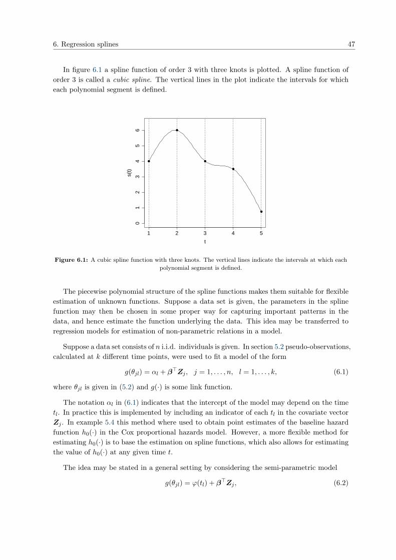
6. Regression splines 47
In figure 6.1 a spline function of order 3 with three knots is plotted. A spline function oforder 3 is called a cubic spline. The vertical lines in the plot indicate the intervals for whicheach polynomial segment is defined.
●
●
●
●
●
1 2 3 4 5
01
23
45
6
t
s(t)
Figure 6.1: A cubic spline function with three knots. The vertical lines indicate the intervals at which eachpolynomial segment is defined.
The piecewise polynomial structure of the spline functions makes them suitable for flexibleestimation of unknown functions. Suppose a data set is given, the parameters in the splinefunction may then be chosen in some proper way for capturing important patterns in thedata, and hence estimate the function underlying the data. This idea may be transferred toregression models for estimation of non-parametric relations in a model.
Suppose a data set consists of n i.i.d. individuals is given. In section 5.2 pseudo-observations,calculated at k different time points, were used to fit a model of the form
g(θjl) = αl + β>Zj , j = 1, . . . , n, l = 1, . . . , k, (6.1)
where θjl is given in (5.2) and g(·) is some link function.
The notation αl in (6.1) indicates that the intercept of the model may depend on the timetl. In practice this is implemented by including an indicator of each tl in the covariate vectorZj . In example 5.4 this method where used to obtain point estimates of the baseline hazardfunction h0(·) in the Cox proportional hazards model. However, a more flexible method forestimating h0(·) is to base the estimation on spline functions, which also allows for estimatingthe value of h0(·) at any given time t.
The idea may be stated in a general setting by considering the semi-parametric model
g(θjl) = ϕ(tl) + β>Zj , (6.2)
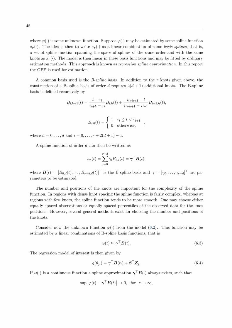
48
where ϕ(·) is some unknown function. Suppose ϕ(·) may be estimated by some spline functionsτ (·). The idea is then to write sτ (·) as a linear combination of some basis splines, that is,a set of spline function spanning the space of splines of the same order and with the sameknots as sτ (·). The model is then linear in these basis functions and may be fitted by ordinaryestimation methods. This approach is known as regression spline approximation. In this reportthe GEE is used for estimation.
A common basis used is the B-spline basis. In addition to the r knots given above, theconstruction of a B-spline basis of order d requires 2(d + 1) additional knots. The B-splinebasis is defined recursively by
Bi,h+1(t) =t− τi
τi+h − τiBi,h(t) +
τi+h+1 − tτi+h+1 − τi+1
Bi+1,h(t),
Bi,0(t) =
{1 τi ≤ t < τi+1
0 otherwise,,
where h = 0, . . . , d and i = 0, . . . , r + 2(d+ 1)− 1.
A spline function of order d can then be written as
sτ (t) =
r+d∑i=0
γiBi,d(t) = γ>B(t),
where B(t) = [B0,d(t), . . . , Br+d,d(t)]> is the B-spline basis and γ = [γ0, . . . , γr+d]
> are pa-rameters to be estimated.
The number and positions of the knots are important for the complexity of the splinefunction. In regions with dense knot spacing the spline function is fairly complex, whereas atregions with few knots, the spline function tends to be more smooth. One may choose eitherequally spaced observations or equally spaced percentiles of the observed data for the knotpositions. However, several general methods exist for choosing the number and positions ofthe knots.
Consider now the unknown function ϕ(·) from the model (6.2). This function may beestimated by a linear combinations of B-spline basis functions, that is
ϕ(t) ≈ γ>B(t). (6.3)
The regression model of interest is then given by
g(θjl) = γ>B(tl) + β>Zj . (6.4)
If ϕ(·) is a continuous function a spline approximation γ>B(·) always exists, such that
sup∣∣ϕ(t)− γ>B(t)
∣∣→ 0, for r →∞,
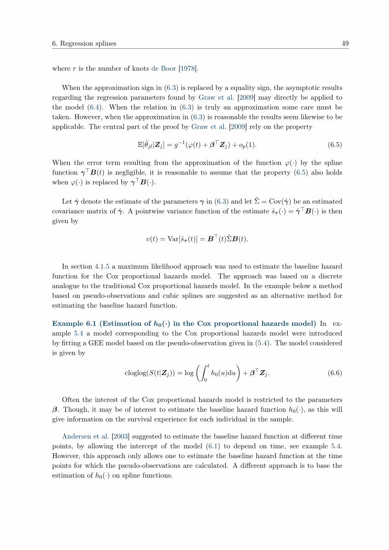
6. Regression splines 49
where r is the number of knots de Boor [1978].
When the approximation sign in (6.3) is replaced by a equality sign, the asymptotic resultsregarding the regression parameters found by Graw et al. [2009] may directly be applied tothe model (6.4). When the relation in (6.3) is truly an approximation some care must betaken. However, when the approximation in (6.3) is reasonable the results seem likewise to beapplicable. The central part of the proof by Graw et al. [2009] rely on the property
E[θjl|Zj ] = g−1(ϕ(t) + β>Zj) + op(1). (6.5)
When the error term resulting from the approximation of the function ϕ(·) by the splinefunction γ>B(t) is negligible, it is reasonable to assume that the property (6.5) also holdswhen ϕ(·) is replaced by γ>B(·).
Let γ denote the estimate of the parameters γ in (6.3) and let Σ = Cov(γ) be an estimatedcovariance matrix of γ. A pointwise variance function of the estimate sτ (·) = γ>B(·) is thengiven by
v(t) = Var[sτ (t)] = B>(t)ΣB(t).
In section 4.1.5 a maximum likelihood approach was used to estimate the baseline hazardfunction for the Cox proportional hazards model. The approach was based on a discreteanalogue to the traditional Cox proportional hazards model. In the example below a methodbased on pseudo-observations and cubic splines are suggested as an alternative method forestimating the baseline hazard function.
Example 6.1 (Estimation of h0(·) in the Cox proportional hazards model) In ex-ample 5.4 a model corresponding to the Cox proportional hazards model were introducedby fitting a GEE model based on the pseudo-observation given in (5.4). The model consideredis given by
cloglog(S(t|Zj)) = log
(∫ t
0h0(u)du
)+ β>Zj . (6.6)
Often the interest of the Cox proportional hazards model is restricted to the parametersβ. Though, it may be of interest to estimate the baseline hazard function h0(·), as this willgive information on the survival experience for each individual in the sample.
Andersen et al. [2003] suggested to estimate the baseline hazard function at different timepoints, by allowing the intercept of the model (6.1) to depend on time, see example 5.4.However, this approach only allows one to estimate the baseline hazard function at the timepoints for which the pseudo-observations are calculated. A different approach is to base theestimation of h0(·) on spline functions.
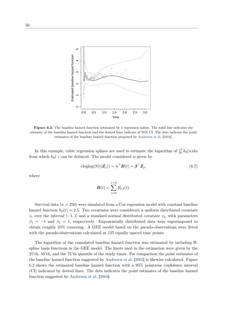
50
0.0 0.5 1.0 1.5 2.0 2.5 3.0
01
23
45
Time
Est
imat
ed b
asel
ine
haza
rd fu
nctio
n
●
●
●●
●
●
●●
●
●
●●
●
●●
●●●
●●
●
●●●●●
●
●
●
●●●
●●●
●
●
●●●●●
●
●●●●●
●●●
●●●●●●
●
●●●●●●●
●●
●●●●●●●●●●●●●
●●●●●
●●
●●●●●●●●●
●●●
●●●
●
●●
●
●
●●
●
●
●
●●
●
● ●●
●
●
●
●
●
●
Figure 6.2: The baseline hazard function estimated by a regression spline. The solid line indicates theestimate of the baseline hazard function and the dotted lines indicate af 95% CI. The dots indicate the point
estimates of the baseline hazard function proposed by Andersen et al. [2003].
In this example, cubic regression splines are used to estimate the logarithm of∫ t
0 h0(u)du
from which h0(·) can be deduced. The model considered is given by
cloglog(S(t|Zj)) = γ>B(t) + β>Zj , (6.7)
where
B(t) =r+3∑i=0
Bi,3(t).
Survival data (n = 250) were simulated from a Cox regression model with constant baselinehazard function h0(t) = 2.5. Two covariates were considered; a uniform distributed covariatez1 over the interval [−1, 1] and a standard normal distributed covariate z2, with parametersβ1 = −1 and β2 = 1, respectively. Exponentially distributed data were superimposed toobtain roughly 25% censoring. A GEE model based on the pseudo-observations were fittedwith the pseudo-observations calculated at 125 equally spaced time points.
The logarithm of the cumulated baseline hazard function was estimated by including B-spline basis functions in the GEE model. The knots used in the estimation were given by the25’th, 50’th, and the 75’th quantile of the study times. For comparison the point estimates ofthe baseline hazard function suggested by Andersen et al. [2003] is likewise calculated. Figure6.2 shows the estimated baseline hazard function with a 95% pointwise confidence interval(CI) indicated by dotted lines. The dots indicates the point estimates of the baseline hazardfunction suggested by Andersen et al. [2003].
6. Regression splines 51
The spline-estimate of the baseline hazard function seems to be agreeable with the truebaseline hazard function h0(t) = 2.5. Though, the estimate is quite fluctuating at the be-ginning of the time scale. In example 5.4 it was seen that the pseudo-observations tend toproduce large standard errors on the regression parameters. A similar trend is seen in figure6.2 with a large 95% CI on the estimated baseline hazard function. The trend is especiallyclear in the region with few observations.
�
7The new pseudo-observation
In chapter 5 jackknife pseudo-observations were introduced as a method for performing gen-eralised linear regression analysis on survival data. The results of the small simulation studyin example 5.4 showed that though the bias of the estimated regression parameters is quitesmall, the parameters have a large variability. A significant part of this variability is related tothe variability in the pseudo-observations, when they are considered as functions over time. Inthis chapter a different estimator is proposed for performing regression analysis on the survivalfunction. The estimator is defined to more precisely resemble the information in the observeddata. The hope is that this information will give more efficient regression estimates.
Consider the pseudo-observation for the survival function in example 5.1 given by
Sj(t) = nS(t)− (n− 1)S−j(t), j = 1, . . . , n (7.1)
where S(·) is the Kaplan-Meier estimator.
Each pseudo-observation (7.1) may be considered as the contribution of individual j tothe Kaplan-Meier estimate of the survival function S(·). Hence, each pseudo-observation isto some extend an estimate of the survival probability for each individual. However, as seenin figure 5.1, each pseudo-observation takes value outside the range of [0, 1] when censoringoccur in the data set. From this it appears that the information given by the observed datais not fully utilised in the definition of the pseudo-observation. For an individual with anobserved event time, the survival probability is estimated by some number above one priorto the observed event time, hereafter the survival probability is estimated by some numberbelow zero. The same holds for an individual with a censored event time; prior to this observedcensored time the survival probability is estimated by some number above one.
A more proper utilisation of the observed data is to estimate the survival probability byconditioning on the observed data. Figure 7.1 shows a plot of an estimator of the probability
52
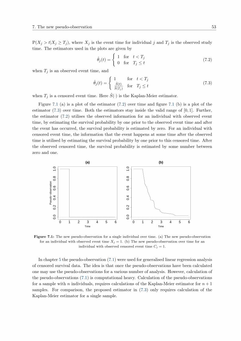
7. The new pseudo-observation 53
P(Xj > t|Xj ≥ Tj), where Xj is the event time for individual j and Tj is the observed studytime. The estimators used in the plots are given by
θj(t) =
{1 for t < Tj0 for Tj ≤ t
(7.2)
when Tj is an observed event time, and
θj(t) =
{1 for t < TjS(t)
S(Tj)for Tj ≤ t
(7.3)
when Tj is a censored event time. Here S(·) is the Kaplan-Meier estimator.
Figure 7.1 (a) is a plot of the estimator (7.2) over time and figure 7.1 (b) is a plot of theestimator (7.3) over time. Both the estimators stay inside the valid range of [0, 1]. Further,the estimator (7.2) utilises the observed information for an individual with observed eventtime, by estimating the survival probability by one prior to the observed event time and afterthe event has occurred, the survival probability is estimated by zero. For an individual withcensored event time, the information that the event happens at some time after the observedtime is utilised by estimating the survival probability by one prior to this censored time. Afterthe observed censored time, the survival probability is estimated by some number betweenzero and one.
0 1 2 3 4 5 6
0.0
0.2
0.4
0.6
0.8
1.0
(a)
Time
Pse
udo−
obse
rvat
ion
0 1 2 3 4 5 6
0.0
0.2
0.4
0.6
0.8
1.0
(b)
Time
Figure 7.1: The new pseudo-observation for a single individual over time. (a) The new pseudo-observationfor an individual with observed event time Xj = 1. (b) The new pseudo-observation over time for an
individual with observed censored event time Cj = 1.
In chapter 5 the pseudo-observation (7.1) were used for generalised linear regression analysisof censored survival data. The idea is that once the pseudo-observations have been calculatedone may use the pseudo-observations for a various number of analysis. However, calculation ofthe pseudo-observations (7.1) is computational heavy. Calculation of the pseudo-observationsfor a sample with n individuals, requires calculations of the Kaplan-Meier estimator for n+ 1
samples. For comparison, the proposed estimator in (7.3) only requires calculation of theKaplan-Meier estimator for a single sample.
54 7.1. Properties of the new pseudo-observation
7.1 Properties of the new pseudo-observation
In this section, some properties regarding the distribution of the new pseudo-observations (7.2)and (7.3) are considered.
First consider the estimator (7.2) for an individual with observed event time, this estimatormay be written in terms of the indicator function θj(t) = 1[Xj > t]. The mean value of thisestimator is then given by
E[θj(t)] = E[1[Xj > t]]
= SX(t).
The variance of this estimator is given by
Var[θj(t)] = SX(t) [1− SX(t)] = SX(t)FX(t).
The estimator (7.3) is a bit more complicated as this estimator depends on both the event timedistribution and the censoring distribution. Let Cj denote the censoring time for individual jand suppose this is independent of the event time Xj . Further, let SX(n) denote the Kaplan-Meier estimator of the event times based on a sample with n individuals. The mean value ofthe estimator (7.3) is then given by
E[θj(t)] = E[1[Xj ∧ Cj > t]] + E
[1[Cj ≤ t ∧Xj ]
SX(n)(t)
SX(n)(Cj)
]
= E[1[Xj > t]1[Cj > t]] + E
[1[Cj ≤ t ∧Xj ]
SX(n)(t)
SX(n)(Cj)
]
= SX(t)SC(t) + E
[1[Cj ≤ t ∧Xj ]
SX(n)(t)
SX(n)(Cj)
]. (7.4)
Consider the second term of the right hand side of (7.4). The Kaplan-Meier estimator is anuniformly consistent estimator of the survival function on the interval [0, t] for all t < u, whereu = sup{t : P(X > t) > 0} Fleming and Harrington [1991]. This means that for t < u thesecond term of (7.4) can be rewritten as
E
[1[Cj ≤ t ∧Xj ]
SX(n)(t)
SX(n)(Cj)
]=
∫ t
0
∫ ∞c
SX(n)(t)
SX(n)(c)dFX(x)dFC(c)
=
∫ t
0
SX(n)(t)
SX(n)(c)
∫ ∞c
1dFX(x)dFC(c)
−−−→n→∞
∫ t
0
SX(t)
SX(c)
∫ ∞c
1dFX(x)dFC(c)
=
∫ t
0
SX(t)
SX(c)SX(c)dFC(c)
= SX(t)FC(t). (7.5)
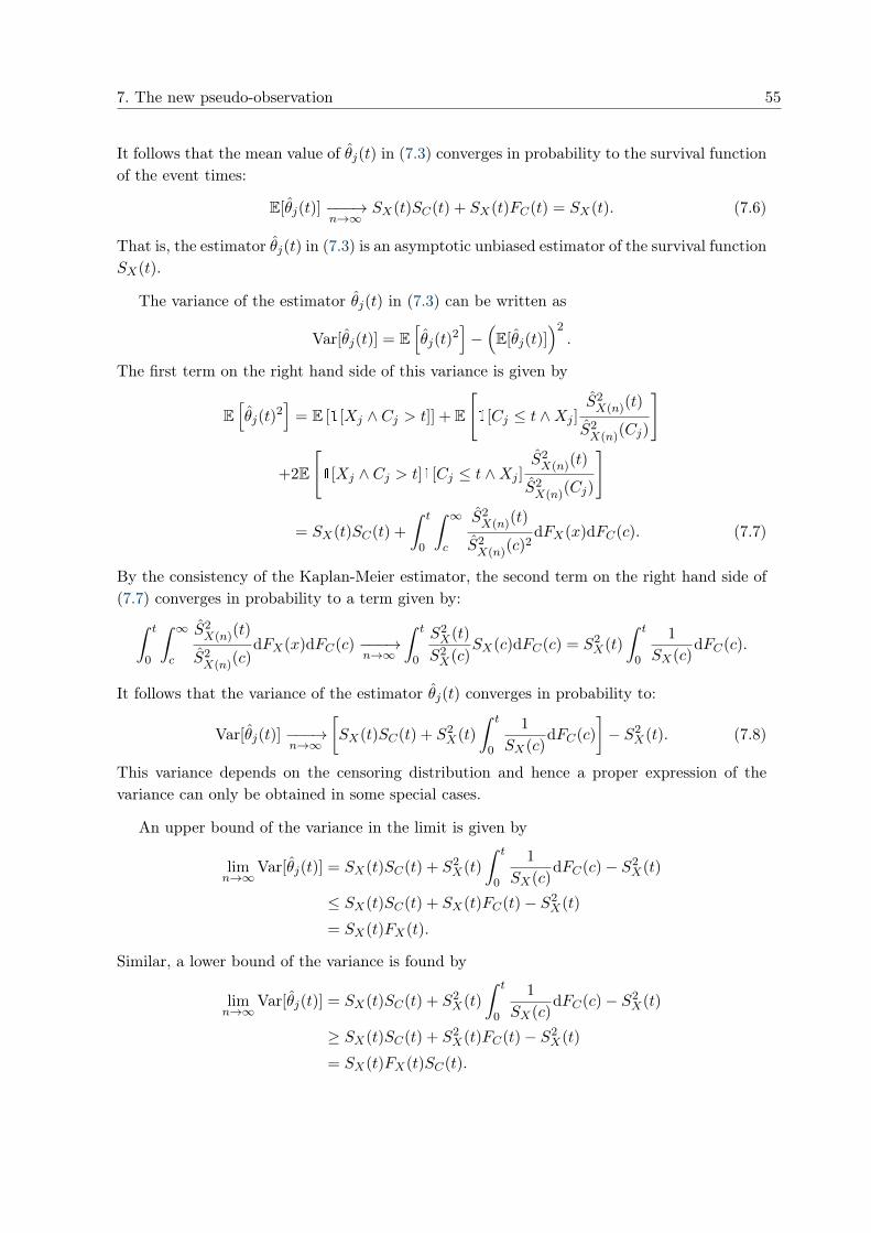
7. The new pseudo-observation 55
It follows that the mean value of θj(t) in (7.3) converges in probability to the survival functionof the event times:
E[θj(t)] −−−→n→∞
SX(t)SC(t) + SX(t)FC(t) = SX(t). (7.6)
That is, the estimator θj(t) in (7.3) is an asymptotic unbiased estimator of the survival functionSX(t).
The variance of the estimator θj(t) in (7.3) can be written as
Var[θj(t)] = E[θj(t)
2]−(E[θj(t)]
)2.
The first term on the right hand side of this variance is given by
E[θj(t)
2]
= E [1[Xj ∧ Cj > t]] + E
[1[Cj ≤ t ∧Xj ]
S2X(n)(t)
S2X(n)(Cj)
]
+2E
[1[Xj ∧ Cj > t]1[Cj ≤ t ∧Xj ]
S2X(n)(t)
S2X(n)(Cj)
]
= SX(t)SC(t) +
∫ t
0
∫ ∞c
S2X(n)(t)
S2X(n)(c)
2dFX(x)dFC(c). (7.7)
By the consistency of the Kaplan-Meier estimator, the second term on the right hand side of(7.7) converges in probability to a term given by:∫ t
0
∫ ∞c
S2X(n)(t)
S2X(n)(c)
dFX(x)dFC(c) −−−→n→∞
∫ t
0
S2X(t)
S2X(c)
SX(c)dFC(c) = S2X(t)
∫ t
0
1
SX(c)dFC(c).
It follows that the variance of the estimator θj(t) converges in probability to:
Var[θj(t)] −−−→n→∞
[SX(t)SC(t) + S2
X(t)
∫ t
0
1
SX(c)dFC(c)
]− S2
X(t). (7.8)
This variance depends on the censoring distribution and hence a proper expression of thevariance can only be obtained in some special cases.
An upper bound of the variance in the limit is given by
limn→∞
Var[θj(t)] = SX(t)SC(t) + S2X(t)
∫ t
0
1
SX(c)dFC(c)− S2
X(t)
≤ SX(t)SC(t) + SX(t)FC(t)− S2X(t)
= SX(t)FX(t).
Similar, a lower bound of the variance is found by
limn→∞
Var[θj(t)] = SX(t)SC(t) + S2X(t)
∫ t
0
1
SX(c)dFC(c)− S2
X(t)
≥ SX(t)SC(t) + S2X(t)FC(t)− S2
X(t)
= SX(t)FX(t)SC(t).
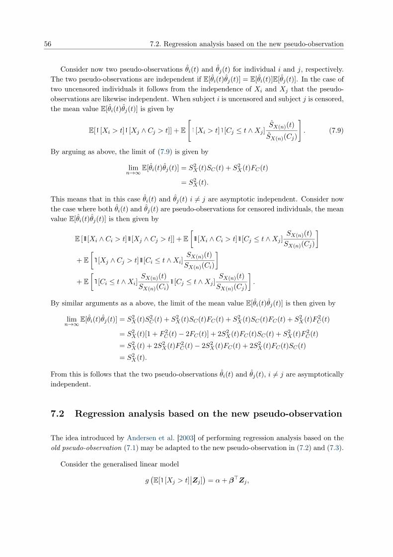
56 7.2. Regression analysis based on the new pseudo-observation
Consider now two pseudo-observations θi(t) and θj(t) for individual i and j, respectively.The two pseudo-observations are independent if E[θi(t)θj(t)] = E[θi(t)]E[θj(t)]. In the case oftwo uncensored individuals it follows from the independence of Xi and Xj that the pseudo-observations are likewise independent. When subject i is uncensored and subject j is censored,the mean value E[θi(t)θj(t)] is given by
E[1[Xi > t]1[Xj ∧ Cj > t]] + E
[1[Xi > t]1[Cj ≤ t ∧Xj ]
SX(n)(t)
SX(n)(Cj)
]. (7.9)
By arguing as above, the limit of (7.9) is given by
limn→∞
E[θi(t)θj(t)] = S2X(t)SC(t) + S2
X(t)FC(t)
= S2X(t).
This means that in this case θi(t) and θj(t) i 6= j are asymptotic independent. Consider nowthe case where both θi(t) and θj(t) are pseudo-observations for censored individuals, the meanvalue E[θi(t)θj(t)] is then given by
E [1[Xi ∧ Ci > t]1[Xj ∧ Cj > t]] + E[1[Xi ∧ Ci > t]1[Cj ≤ t ∧Xj ]
SX(n)(t)
SX(n)(Cj)
]+ E
[1[Xj ∧ Cj > t]1[Ci ≤ t ∧Xi]
SX(n)(t)
SX(n)(Ci)
]+ E
[1[Ci ≤ t ∧Xi]
SX(n)(t)
SX(n)(Ci)1[Cj ≤ t ∧Xj ]
SX(n)(t)
SX(n)(Cj)
].
By similar arguments as a above, the limit of the mean value E[θi(t)θj(t)] is then given by
limn→∞
E[θi(t)θj(t)] = S2X(t)S2
C(t) + S2X(t)SC(t)FC(t) + S2
X(t)SC(t)FC(t) + S2X(t)F 2
C(t)
= S2X(t)[1 + F 2
C(t)− 2FC(t)] + 2S2X(t)FC(t)SC(t) + S2
X(t)F 2C(t)
= S2X(t) + 2S2
X(t)F 2C(t)− 2S2
X(t)FC(t) + 2S2X(t)FC(t)SC(t)
= S2X(t).
From this is follows that the two pseudo-observations θi(t) and θj(t), i 6= j are asymptoticallyindependent.
7.2 Regression analysis based on the new pseudo-observation
The idea introduced by Andersen et al. [2003] of performing regression analysis based on theold pseudo-observation (7.1) may be adapted to the new pseudo-observation in (7.2) and (7.3).
Consider the generalised linear model
g(E[1[Xj > t]
∣∣Zj ]) = α+ β>Zj ,
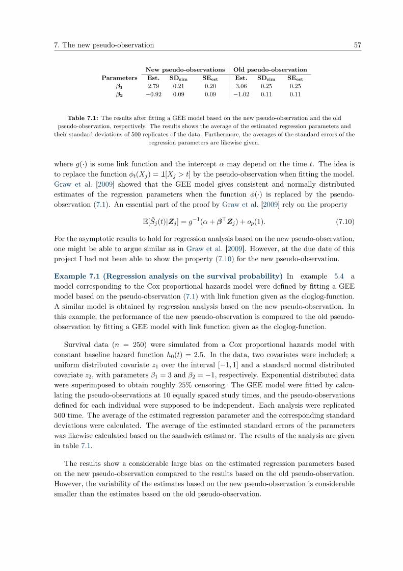
7. The new pseudo-observation 57
New pseudo-observations Old pseudo-observationParameters Est. SDsim SEest Est. SDsim SEest
β1 2.79 0.21 0.20 3.06 0.25 0.25
β2 −0.92 0.09 0.09 −1.02 0.11 0.11
Table 7.1: The results after fitting a GEE model based on the new pseudo-observation and the oldpseudo-observation, respectively. The results shows the average of the estimated regression parameters and
their standard deviations of 500 replicates of the data. Furthermore, the averages of the standard errors of theregression parameters are likewise given.
where g(·) is some link function and the intercept α may depend on the time t. The idea isto replace the function φt(Xj) = 1[Xj > t] by the pseudo-observation when fitting the model.Graw et al. [2009] showed that the GEE model gives consistent and normally distributedestimates of the regression parameters when the function φ(·) is replaced by the pseudo-observation (7.1). An essential part of the proof by Graw et al. [2009] rely on the property
E[Sj(t)|Zj ] = g−1(α+ β>Zj) + op(1). (7.10)
For the asymptotic results to hold for regression analysis based on the new pseudo-observation,one might be able to argue similar as in Graw et al. [2009]. However, at the due date of thisproject I had not been able to show the property (7.10) for the new pseudo-observation.
Example 7.1 (Regression analysis on the survival probability) In example 5.4 amodel corresponding to the Cox proportional hazards model were defined by fitting a GEEmodel based on the pseudo-observation (7.1) with link function given as the cloglog-function.A similar model is obtained by regression analysis based on the new pseudo-observation. Inthis example, the performance of the new pseudo-observation is compared to the old pseudo-observation by fitting a GEE model with link function given as the cloglog-function.
Survival data (n = 250) were simulated from a Cox proportional hazards model withconstant baseline hazard function h0(t) = 2.5. In the data, two covariates were included; auniform distributed covariate z1 over the interval [−1, 1] and a standard normal distributedcovariate z2, with parameters β1 = 3 and β2 = −1, respectively. Exponential distributed datawere superimposed to obtain roughly 25% censoring. The GEE model were fitted by calcu-lating the pseudo-observations at 10 equally spaced study times, and the pseudo-observationsdefined for each individual were supposed to be independent. Each analysis were replicated500 time. The average of the estimated regression parameter and the corresponding standarddeviations were calculated. The average of the estimated standard errors of the parameterswas likewise calculated based on the sandwich estimator. The results of the analysis are givenin table 7.1.
The results show a considerable large bias on the estimated regression parameters basedon the new pseudo-observation compared to the results based on the old pseudo-observation.However, the variability of the estimates based on the new pseudo-observation is considerablesmaller than the estimates based on the old pseudo-observation.
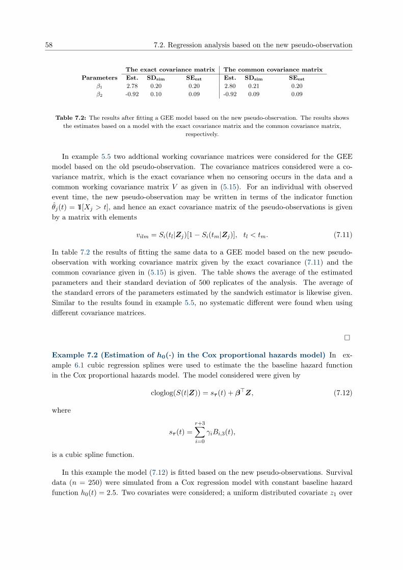
58 7.2. Regression analysis based on the new pseudo-observation
The exact covariance matrix The common covariance matrixParameters Est. SDsim SEest Est. SDsim SEest
β1 2.78 0.20 0.20 2.80 0.21 0.20β2 -0.92 0.10 0.09 -0.92 0.09 0.09
Table 7.2: The results after fitting a GEE model based on the new pseudo-observation. The results showsthe estimates based on a model with the exact covariance matrix and the common covariance matrix,
respectively.
In example 5.5 two addtional working covariance matrices were considered for the GEEmodel based on the old pseudo-observation. The covariance matrices considered were a co-variance matrix, which is the exact covariance when no censoring occurs in the data and acommon working covariance matrix V as given in (5.15). For an individual with observedevent time, the new pseudo-observation may be written in terms of the indicator functionθj(t) = 1[Xj > t], and hence an exact covariance matrix of the pseudo-observations is givenby a matrix with elements
vilm = Si(tl|Zj)[1− Si(tm|Zj)], tl < tm. (7.11)
In table 7.2 the results of fitting the same data to a GEE model based on the new pseudo-observation with working covariance matrix given by the exact covariance (7.11) and thecommon covariance given in (5.15) is given. The table shows the average of the estimatedparameters and their standard deviation of 500 replicates of the analysis. The average ofthe standard errors of the parameters estimated by the sandwich estimator is likewise given.Similar to the results found in example 5.5, no systematic different were found when usingdifferent covariance matrices.
�
Example 7.2 (Estimation of h0(·) in the Cox proportional hazards model) In ex-ample 6.1 cubic regression splines were used to estimate the the baseline hazard functionin the Cox proportional hazards model. The model considered were given by
cloglog(S(t|Z)) = sτ (t) + β>Z, (7.12)
where
sτ (t) =r+3∑i=0
γiBi,3(t),
is a cubic spline function.
In this example the model (7.12) is fitted based on the new pseudo-observations. Survivaldata (n = 250) were simulated from a Cox regression model with constant baseline hazardfunction h0(t) = 2.5. Two covariates were considered; a uniform distributed covariate z1 over
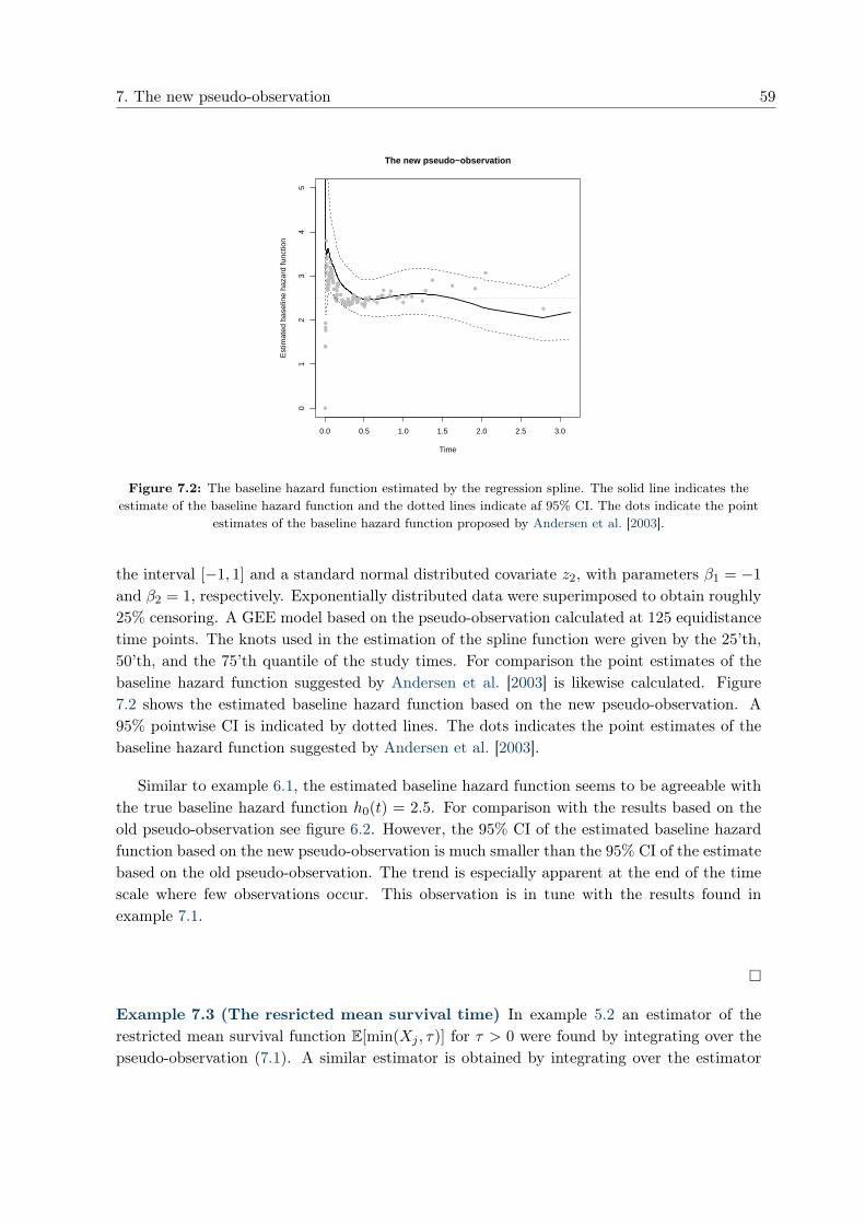
7. The new pseudo-observation 59
0.0 0.5 1.0 1.5 2.0 2.5 3.0
01
23
45
The new pseudo−observation
Time
Est
imat
ed b
asel
ine
haza
rd fu
nctio
n
●
●●
●
●●
●
●●
●
●
●●
●
●
●
●●●●●●●●●●
●●●
●●●●
●
●
●
●●
●●●●●
●
●●●●●●
●●
●●●●●●●
●
●●●●●●
●●
●●●●
●●●●●●●●●
●●●●●
●●●●●●●●●●●
●●●●●●
●●
●●
● ●●
●
●
●
●●
●
● ●
●
●
●
●●
●
●
Figure 7.2: The baseline hazard function estimated by the regression spline. The solid line indicates theestimate of the baseline hazard function and the dotted lines indicate af 95% CI. The dots indicate the point
estimates of the baseline hazard function proposed by Andersen et al. [2003].
the interval [−1, 1] and a standard normal distributed covariate z2, with parameters β1 = −1
and β2 = 1, respectively. Exponentially distributed data were superimposed to obtain roughly25% censoring. A GEE model based on the pseudo-observation calculated at 125 equidistancetime points. The knots used in the estimation of the spline function were given by the 25’th,50’th, and the 75’th quantile of the study times. For comparison the point estimates of thebaseline hazard function suggested by Andersen et al. [2003] is likewise calculated. Figure7.2 shows the estimated baseline hazard function based on the new pseudo-observation. A95% pointwise CI is indicated by dotted lines. The dots indicates the point estimates of thebaseline hazard function suggested by Andersen et al. [2003].
Similar to example 6.1, the estimated baseline hazard function seems to be agreeable withthe true baseline hazard function h0(t) = 2.5. For comparison with the results based on theold pseudo-observation see figure 6.2. However, the 95% CI of the estimated baseline hazardfunction based on the new pseudo-observation is much smaller than the 95% CI of the estimatebased on the old pseudo-observation. The trend is especially apparent at the end of the timescale where few observations occur. This observation is in tune with the results found inexample 7.1.
�
Example 7.3 (The resricted mean survival time) In example 5.2 an estimator of therestricted mean survival function E[min(Xj , τ)] for τ > 0 were found by integrating over thepseudo-observation (7.1). A similar estimator is obtained by integrating over the estimator
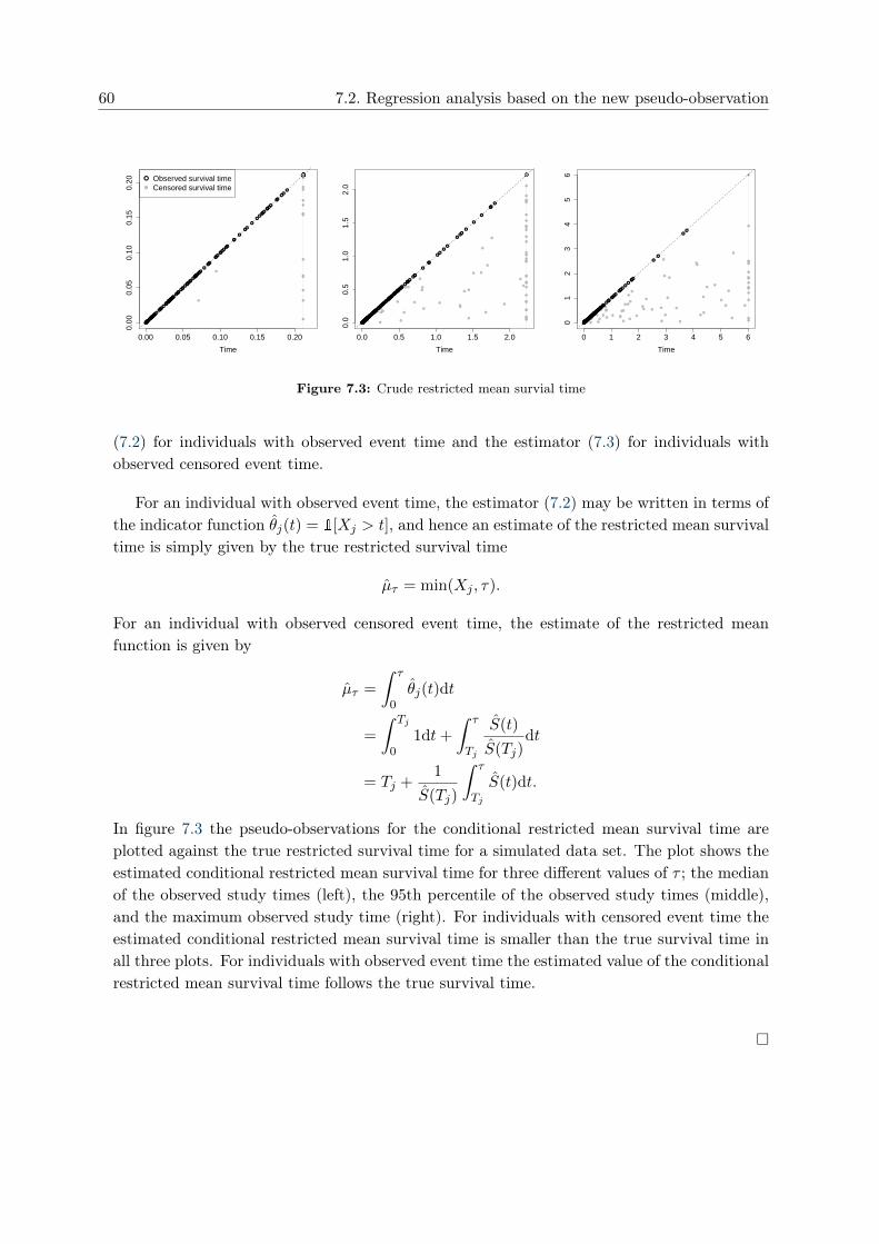
60 7.2. Regression analysis based on the new pseudo-observation
●●●●●●●●●●● ●●●●●●●
●●●●●●●●
●●●●
●●
●●●●●●●●●●
● ●●●●●●●●●●
●●●●
●●●●●●●●●●●
●● ●●●●● ●●●●●
● ●
●●●●
●●●
●●●
●●●●
●●
●
●●
●
●● ●●●
●●●
●●●● ●
●●●●
●● ●
●
●●●●●●●●●●●●●●●●●●●●●●●●●●●●●●●●●●●●●●●●●●●●●●●●●●●●●●●●●●●●●●●●●●●●●●●●●●●●●●●●●●●●●●●●●●●●●●●●●●●●●●●●●●●●●●●●●●●●●●●●●●●●●●●
0.00 0.05 0.10 0.15 0.20
0.00
0.05
0.10
0.15
0.20
Time
●
●
Observed survival timeCensored survival time
●●●●●●●●●●● ●●●●●●●●●●●●●●●●●●●●●●●●●●●●●●● ● ●●●●●●●●●●●●●● ●●●●●●●●●●●●●
●●●●● ●●●●●●●●●●● ●●●●●●●●●●●●●●●●●● ●● ●●●●●●●● ● ●●●●●● ●●
●● ●●●●●●● ●●● ●●●● ●●● ●● ●●● ●●●●●
●●●●●●● ●●●●
●●●● ●●●●● ● ●●●●● ●● ●●●●
●●
●●●●●● ●●
● ●●●●● ●
●●
●● ●●●
●●● ●
● ●●
●
●● ●●●
●●●●
●●
● ●
●●● ●
●●
●
●
●●●●●●●●●●●●●
0.0 0.5 1.0 1.5 2.00.
00.
51.
01.
52.
0Time
●●●●●●●●●●● ●●●●●●●●●●●●●●●●●●●●●●●●●●●●●●●● ●●●●●●●●●●●●●● ●●●●●●●●●●●●● ●●●●● ●●●●●●●●●●● ●●●●●●●●●●●●●●●●●●●● ●●●●●●●●●●●●●●● ●●●● ●●●● ●●● ●●● ●●●● ●●● ●● ●●●●●●●●●●●●●●●
●●●●●●●●●●●●● ● ●●●●● ●● ●●●● ●● ●●●●●●
●●● ●●●● ● ●● ●●● ● ●●
●●● ●● ●●●
●● ●●●●● ●●
● ●● ●
●●● ●● ●●
●
●●●●●● ●
●●
●●
●
●
0 1 2 3 4 5 6
01
23
45
6
Time
Figure 7.3: Crude restricted mean survial time
(7.2) for individuals with observed event time and the estimator (7.3) for individuals withobserved censored event time.
For an individual with observed event time, the estimator (7.2) may be written in terms ofthe indicator function θj(t) = 1[Xj > t], and hence an estimate of the restricted mean survivaltime is simply given by the true restricted survival time
µτ = min(Xj , τ).
For an individual with observed censored event time, the estimate of the restricted meanfunction is given by
µτ =
∫ τ
0θj(t)dt
=
∫ Tj
01dt+
∫ τ
Tj
S(t)
S(Tj)dt
= Tj +1
S(Tj)
∫ τ
Tj
S(t)dt.
In figure 7.3 the pseudo-observations for the conditional restricted mean survival time areplotted against the true restricted survival time for a simulated data set. The plot shows theestimated conditional restricted mean survival time for three different values of τ ; the medianof the observed study times (left), the 95th percentile of the observed study times (middle),and the maximum observed study time (right). For individuals with censored event time theestimated conditional restricted mean survival time is smaller than the true survival time inall three plots. For individuals with observed event time the estimated value of the conditionalrestricted mean survival time follows the true survival time.
�

8Discussion and conclusion
The inherent structure of survival data entail that standard statistical models cannot be usedfor analysis this type of data. Especially the occurrence of censored data is a technicality,which must be dealt with when analysing survival data. Survival data is often summarizedthrough the hazard function and the survival function. These functions serve to describeimportant aspects of the survival experience in a given data set. The mean survival time isanother parameter of great interest, which gives the expected time until some event occur.However, due to right censoring the mean survival time is often ill determined beyond a certainrange. A related quantity is the restricted mean survival time which is less sensitive to rightcensoring. Traditional regression analysis of survival data is hence concentrated on relatingcovariates to these functions, with the hazard function playing the most prominent role. Oftenthe functions themself are not of primary interest. From a practical point of view, one is oftenmore interested in the effect of the covariates. From this perspective, semi-parametric modelshave been used as the primary tool for regression analysis of survival data; here the Coxproportional hazards model is one of the most popular methods.
In this project jackknife pseudo-observations have been studied as a tool for analysingsurvival data. Pseudo-observations adress the problem of not having appropriate observationsfor all individuals in the study. The approach is based on a set of pseudo-observations definedfor each individual in the study. The pseudo-observations allow one to analyse the effect of aset of covariates on the event times by models more general than the standard models used forsurvival data. In section 5.2 the GEE approach based on pseudo-observations were used to fita generalised linear model for functions of the event times. The advantage of this approachis that it allows one to model the event times by generalised linear models without specifyinga full parametric model. The justification for the use of pseudo-observations in the GEEapproach is based on some neat results found by Graw et al. [2009] concerning the estimatedregression parameters.
In section 5.2, regression analysis based on pseudo observations were compared to thetraditional Cox proportional hazards model. A small simulation study showed that the model
62
8. Discussion and conclusion 63
based on pseudo-observations is not competitive to this standard method of analysing survivaldata. The weakness of the pseudo-observation approach is mainly the relative large standarderrors of the estimated regression parameters; this variation is related to the variability in theset of pseudo-observations. The question regarding the number of time points for which thepseudo-observations are calculated were also considered. The results showed that increasingthe number of equidistant time points did not increase the performance of the model. However,in a general setting it is reasonable to believe that the number and position of the time pointswill affect the performance of the regression analysis. For the regression analysis to performwell, the survival structure in the true event distribution must be captured by the pseudo-observations. Hence, improper positions of the pseudo-observations will reasonable effect theefficiency of the analysis.
In chapter 6 cubic regression splines based on pseudo-observations were used to estimatethe baseline hazard function of the Cox proportional hazards model. This is a simple methodwhich allow for a flexible estimation of the baseline hazard function. A simple example witha constant baseline hazard function was considered. The results show that the approach is areliable method for estimation of this hazard function. In general cubic regression splines areflexible functions and it is reasonable be believe that the method will perform well for morecomplex functions. In chapter 6 it was argued that when the error term resulting from thespline approximation of the unknown function is negligible, the resulting regression parameterswill possess the same desirable properties found by Graw et al. [2009]. However, if the splineapproximation introduce a large error term, a corresponding bias on the estimated parametersis expected.
In chapter 7 a new pseudo-observation was proposed for estimating survival probabilities.The motivation behind the definition of this new pseudo-observation is the large estimatedvariance obtained from regression analysis based the old pseudo-observation. The new pseudo-observation was defined to more proper capture the information given by the observed data. Asmall simulation study showed that the new pseudo-observation tend to give estimated regres-sion parameters with less variability compared to the old pseudo-observation. Though, a largebias on the regression parameters resulting from this new pseudo-observation was observed.During the period of this project attempt has been made to prove asymptotic properties forthe new pseudo-observation similar to those found by Graw et al. [2009]. However, a biasrelated to the censoring distributed was encountered. This suggests that the range of the newpseudo-observations might be inadequate for compensation of the uncertainty related to thesurvival experience for censored individuals. In contrast, the definition of the old pseudo-observation causes this estimator to take values outside the range of [0, 1], from which thevariability in the regression results is caused by. However, these unusually values seem tocompensate each other to produce estimates capturing the information in the true underlyingevent distribution. This discussion suggests a trade-off between bias and variation on theestimated regression results. The old pseudo-observation seems to produce estimates whichon average produce accurate estimates. However, the variability makes these estimates lessreliable in a single sample. The potential of the new pseudo-observation rely on its ability toproduce regression results with high reliability, though accounting for the bias.
64
One may consider to reduce the bias of the estimated regression parameters resulting fromthe new pseudo-observation by a two-step estimation method. The first step is to estimatesome initial regression parameters based on the sample of individuals with observed event timeonly. The new pseudo-observation for individuals with observed event time is simply givenby θj(t) = 1[Xj > t]. It follows directly from the results of Liang and Zeger [1986] that thisestimator will produce consistent estimates of the true regression parameters, though a largevariance is expected due to omitting censored individuals. The next step is then to predictthe value of S(·|Zj) for censored individuals, based on these initial parameters. The newpseudo-observation for censored individuals given in (7.3) may then be modified as follows
θj(t) =
{1 for t < CjS(t|Zj)S(Cj |Zj) for Cj ≤ t
.
The final regression analysis is then based on all individuals in the study, including censoredindividuals. Though, rather than using the estimator proposed in chapter 7, the analysisis based on the above estimator for censored individuals. This estimator will increase thecomputational burden, however, the bias of the resulting regression parameters is expected todecrease will maintaining the small variance. Due to time pressure, this method has not beenconsidered in the study.
The generalisation of jackknife pseudo-observations for analysis of survival data a is relativenew method with the first article printed in 2003 (Andersen et al. [2003]). The method is notyet fully developed, and more reseach is needed to answer a number of unanswered questions,like the best choice regarding the number and position of the time points for which the pseudo-observations are calculated. In this project, the efficiency of the pseudo-observations has beenaddressed together with some practical considerations for capable regression results. The ideaof pseudo-observations for survival analysis has been proposed in a general setting, thoughstudies of the pseudo-observations have so far been restricted to three special estimators.The results found in this project show that the pseudo-observations have a potential as ageneral method for analysing survival data in a number of ways. The potential of the pseudo-observation relies on their ability to generalise survival data by introducing proper observationsfor all individuals in the study. This allows for analysis of survival data by methods usuallyrestricted to data with full information. The approach based on pseudo-observations is notcompetetive to traditional methods used to analyse survival data. However, the pseudo-observations alows for general statistical methods to supplement the tradtional survival datamethods.

9Bibliography
Andersen and Perme, 2010. Per Kragh Andersen and Maja Pohar Perme. Pseudo-observations in survival analysis. Statistical Methods in Medical Research, 19(1), 71–99,2010.
Andersen, Borgan, Gill, and Keiding, 1993. Per Kragh Andersen, Ørnulf Borgan,Richard D. Gill, and Niels Keiding. Statistical models based on counting processes. Springer-Verlag, 1993. ISBN 0-387-97872-0.
Andersen, Klein, and Rosthøj, 2003. Per Kragh Andersen, John P. Klein, and SusanneRosthøj. Generalised linear models for correlated pseudo-observations, with applications tomulti-state models. Biometrika, 90(1), 15–27, 2003.
Azzalini, 2002. A. Azzalini. Statistical Inference Based on the likelihood. Chapman & Hall,2002. ISBN 978-0-4126-0650-2.
Binder, Gerds, and Andersen, 2012. Nadine Binder, Thomas A. Gerds, and Per KraghAndersen. Pseudo-observations for competing risks with covariates dependent censoring -research report 12/06, Department of Biostatistics University of Copenhagen, 2012.
Breslow, 1974. N. Breslow. Covariance Analysis of Censored Survival Data. Biometrics, 30(1), 89–99, 1974.
Cox, 1972. D.R. Cox. Regression Models and Life-Tables. Journal of the Royal StatisticalSociety. Series B (Methodological), 34(2), 187–220, 1972.
Cox, 1975. D.R. Cox. Partial likelihood. Biometrika, 62(2), 269–276, 1975.
Boor, 1978. Carl de Boor. A practical guide to splines. Springer, 1978. ISBN 0-387-90356-9.
Efron, 1977. Bradley Efron. The Efficiency of Cox’s Likelihood Function for Censored Data.Journal of the American Statistical Association, 72(359), 557–565, 1977.
66
9. Bibliography 67
Fitzmaurice, Davidian, Verbeke, and Molenberghs, 2008. Garrett Fitzmaurice, MarieDavidian, Geert Verbeke, and Geert Molenberghs. Longitudinal data analysis. Chapman &Hall/CRC, 2008. ISBN 978-1-58488-658-7.
Fleming and Harrington, 1991. Thomas R. Fleming and David P. Harrington. Countingprocesses and survival analysis. Chichester: Wiley, 1991. ISBN 0-471-52218-x.
Graw, Gerds, and Schumacher, 2009. Frederik Graw, Thomas A. Gerds, and MartinSchumacher. On pseudo-values for regression analysis in competing risks models. LifetimeData Analysis, 15(2), 241 –255, 2009.
Green and Silverman, 1994. P.J. Green and B.W. Silverman. Nonparametric regressionand generalized linear models. London: Chapman & Hall, 1994. ISBN 0-412-30040-0.
Hastie, Tibshirani, and Friedman, 2001. Trevor Hastie, Robert Tibshirani, and JeromeFriedman. The elements of statistical learning : data mining, inference, and prediction.New York: Springer, 2001. ISBN 0-387-95284-5.
Hosmer and Lemeshow, 1999. David W. Hosmer and Stanley Lemeshow. Applied survivalanalysis: regression modelling of time to event data. Wiley, 1999. ISBN 0-471-15410-5.
Kalbfleisch and Prentice, 2002. John D. Kalbfleisch and Ross L. Prentice. The statisticalanalysis of failure time data. Wiley-Interscience, 2002. ISBN 978-0-471-36357-6.
Klein and Andersen, 2005. John P. Klein and Per Kragh Andersen. Regression Modelingof Competing Risks Data Based on Pseudovalues of the Cumulative Incidence Function.Biometrics, 61(1), 223–229, 2005.
Klein and Moeschberger, 1997. John P. Klein and Melvin L. Moeschberger. Survivalanalysis: techniques for censored and truncated data. Springer-Verlag, 1997. ISBN 0-387-94829-5.
Liang and Zeger, 1986. Kung-Yee Liang and Scott L. Zeger. Longitudinal data analysisusing generalized linear models. Biometrika, 73(1), 13–22, 1986.
Miller, 1974. Rupert G. Miller. The jackknife - a review. Biometrika, 61(1), 1–15, 1974.
Perme and Andersen, 2008. Maja Pohar Perme and Per Kragh Andersen. Checking hazardregression models using pseudo-observations. Statistics in medicine, 27(25), 5309–28, 2008.
Tukey, 1958. J. W. Tukey. Bias and confidence in not quite large samples (abstract). Annalsof Mathematical Statistics, 29, 614, 1958.
AAppendix
A.1 The cumulative incidence function
The section is written based on Binder et al. [2012].
In chapter 5 the Aalen-Johansen estimator were used to define pseudo-observations forthe cumulative cause-r incidence function in a competing risks analysis. In section 5.1 itwas claimed that in the case of no censoring, the pseudo-observation reduces to an indicatorfunction Fjr(t) = 1[Xj ≤ t, εj = r]. The justic for this is given below. Suppose a sample withn individuals are given and let Nr(·) be the counting process defined by
Nr(t) =
n∑j=1
1[Tj ≤ t, δj = 1, εj = r],
where Tj = min(Xj , Cj), δj = 1[Xj ≤ Cj ], and εj indicates which competing risks caused theevent. Further, let Y (·) denote the risk set and let Hr(·) denote the Nelson-Aalen estimatorfor the cause-r specified hazard function.
Consider the Aalen-Johansen estimator of the cause-r cumulative incidence function givenby
Fr(t) =
∫ t
0
∏v<u
(1−
∑Kr=1 dNr(v)
Y (v)
)dHr(u)
=
∫ t
0SX(u−)dHr(u),
where S(·) denote the Kaplan-Meier estimator of the survival function for all event times inthe study and K is the number of competing risks. It can be shown that Y (t)
n = SX(t−)SC(t−),
68
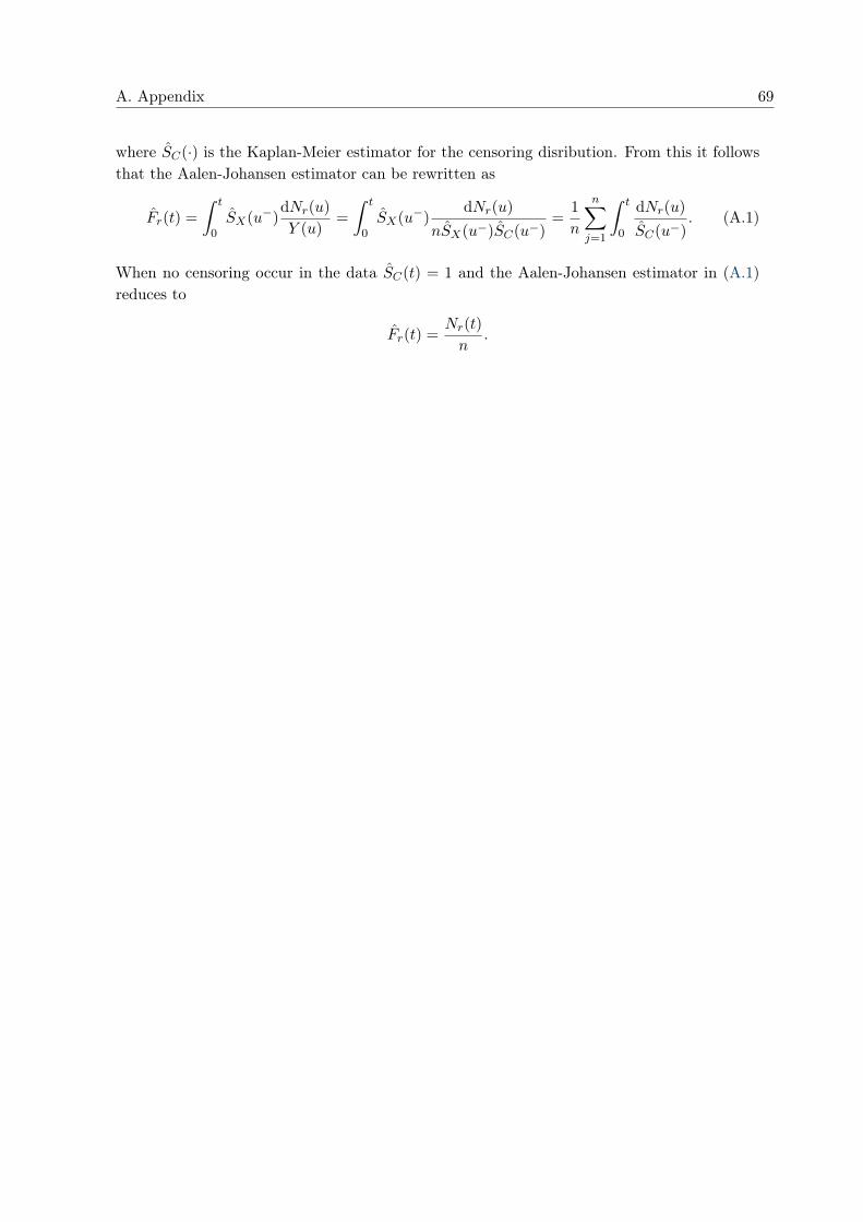
A. Appendix 69
where SC(·) is the Kaplan-Meier estimator for the censoring disribution. From this it followsthat the Aalen-Johansen estimator can be rewritten as
Fr(t) =
∫ t
0SX(u−)
dNr(u)
Y (u)=
∫ t
0SX(u−)
dNr(u)
nSX(u−)SC(u−)=
1
n
n∑j=1
∫ t
0
dNr(u)
SC(u−). (A.1)
When no censoring occur in the data SC(t) = 1 and the Aalen-Johansen estimator in (A.1)reduces to
Fr(t) =Nr(t)
n.