PS598 - Mathematics for Political Scientists - Section Notes

(Extremely Abridged!)

Jason S. Davis

Fall 2014

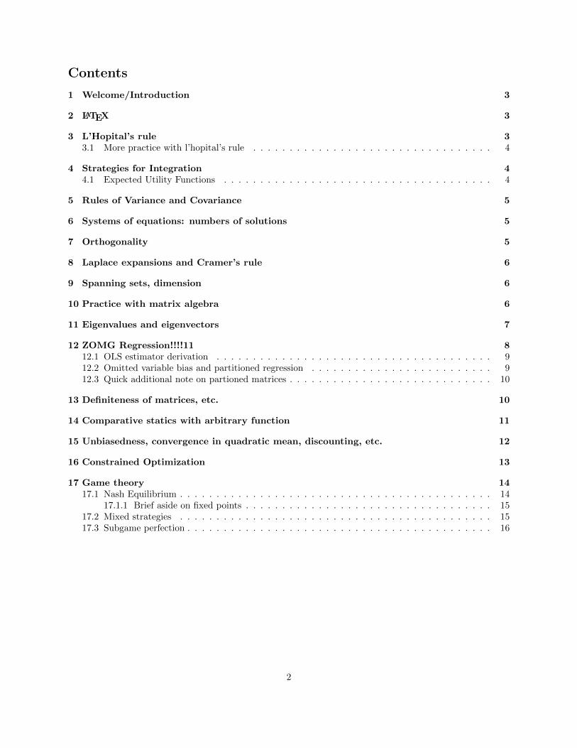
Contents

1 Welcome/Introduction 3

2 LATEX 3

3 L’Hopital’s rule 33.1 More practice with l’hopital’s rule . . . . . . . . . . . . . . . . . . . . . . . . . . . . . . . . . 4

4 Strategies for Integration 44.1 Expected Utility Functions . . . . . . . . . . . . . . . . . . . . . . . . . . . . . . . . . . . . . 4

5 Rules of Variance and Covariance 5

6 Systems of equations: numbers of solutions 5

7 Orthogonality 5

8 Laplace expansions and Cramer’s rule 6

9 Spanning sets, dimension 6

10 Practice with matrix algebra 6

11 Eigenvalues and eigenvectors 7

12 ZOMG Regression!!!!11 812.1 OLS estimator derivation . . . . . . . . . . . . . . . . . . . . . . . . . . . . . . . . . . . . . . 912.2 Omitted variable bias and partitioned regression . . . . . . . . . . . . . . . . . . . . . . . . . 912.3 Quick additional note on partioned matrices . . . . . . . . . . . . . . . . . . . . . . . . . . . . 10

13 Definiteness of matrices, etc. 10

14 Comparative statics with arbitrary function 11

15 Unbiasedness, convergence in quadratic mean, discounting, etc. 12

16 Constrained Optimization 13

17 Game theory 1417.1 Nash Equilibrium . . . . . . . . . . . . . . . . . . . . . . . . . . . . . . . . . . . . . . . . . . . 14

17.1.1 Brief aside on fixed points . . . . . . . . . . . . . . . . . . . . . . . . . . . . . . . . . . 1517.2 Mixed strategies . . . . . . . . . . . . . . . . . . . . . . . . . . . . . . . . . . . . . . . . . . . 1517.3 Subgame perfection . . . . . . . . . . . . . . . . . . . . . . . . . . . . . . . . . . . . . . . . . . 16

2

1 Welcome/Introduction

• Jason Davis - E-mail: jasonsd@umich.edu - Office: Haven Hall 7730 - Telephone: (write in class)

• Most of you know me from math camp.

• Will have office hours immediately after sections generally, though not today!

• Besides textbooks, one other useful resource for a lot of this math is Martin Osborne’s (a game theoristat University of Toronto) math tutorial. It is references by a lot of economists and political scientists,and his game theory textbooks are also super popular:http://www.economics.utoronto.ca/osborne/MathTutorial/

2 LATEX

• Good idea to get LATEX.

• Can post some notes on how to get used to it. But a bit of an overview...

• Lots of different editors. MiKTeX is the most common implementation.

• WinEDT used by some. TeXnicCenter. Various others.

• Not WYSIWYG. Over time, easy to get used to the typsetting.

• Very good for math. Good for other stuff too.

• Useful resources for learning LATEXand R can be found (courtesy of Rochester’s political science de-partment) at the following link:http://www.rochester.edu/college/psc/thestarlab/resources

3 L’Hopital’s rule

• We learned a number of diferent ways of computing derivatives.

• Can also use derivatives to help evaluate limits. L’hopital’s rule allows this

• Say you have two functions that tend to zero, or tend to positive infinity, as they approach either aconstant or infinity.

• Examples: limx→c f(x) =∞ and limx→c g(x) =∞

• More examples: limx→∞ f(x) = 0 and limx→∞ g(x) = 0

• L’hopital’s rule tells us that limx→cf(x)g(x) = limx→c

f ′(x)g′(x)

• So long as g′(x) 6= 0 for all x 6= c

• Examples: limx→15x4−4x2−110−x−9x3

• limx→∞ex

x2 . Apply twice!

3

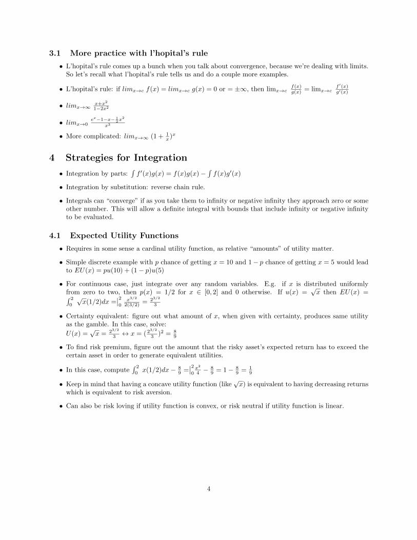
3.1 More practice with l’hopital’s rule

• L’hopital’s rule comes up a bunch when you talk about convergence, because we’re dealing with limits.So let’s recall what l’hopital’s rule tells us and do a couple more examples.

• L’hopital’s rule: if limx→c f(x) = limx→c g(x) = 0 or = ±∞, then limx→cf(x)g(x) = limx→c

f ′(x)g′(x)

• limx→∞x+x2

1−2x2

• limx→0ex−1−x− 1

2x2

x3

• More complicated: limx→∞ (1 + 1x )x

4 Strategies for Integration

• Integration by parts:∫f ′(x)g(x) = f(x)g(x)−

∫f(x)g′(x)

• Integration by substitution: reverse chain rule.

• Integrals can “converge” if as you take them to infinity or negative infinity they approach zero or someother number. This will allow a definite integral with bounds that include infinity or negative infinityto be evaluated.

4.1 Expected Utility Functions

• Requires in some sense a cardinal utility function, as relative “amounts” of utility matter.

• Simple discrete example with p chance of getting x = 10 and 1− p chance of getting x = 5 would leadto EU(x) = pu(10) + (1− p)u(5)

• For continuous case, just integrate over any random variables. E.g. if x is distributed uniformlyfrom zero to two, then p(x) = 1/2 for x ∈ [0, 2] and 0 otherwise. If u(x) =

√x then EU(x) =∫ 2

0

√x(1/2)dx =

∣∣20

x3/2

2(3/2) = 23/2

3

• Certainty equivalent: figure out what amount of x, when given with certainty, produces same utilityas the gamble. In this case, solve:

U(x) =√x = 23/2

3 ↔ x = ( 23/2

3 )2 = 89

• To find risk premium, figure out the amount that the risky asset’s expected return has to exceed thecertain asset in order to generate equivalent utilities.

• In this case, compute∫ 2

0x(1/2)dx− 8

9 =∣∣20x2

4 −89 = 1− 8

9 = 19

• Keep in mind that having a concave utility function (like√x) is equivalent to having decreasing returns

which is equivalent to risk aversion.

• Can also be risk loving if utility function is convex, or risk neutral if utility function is linear.

4

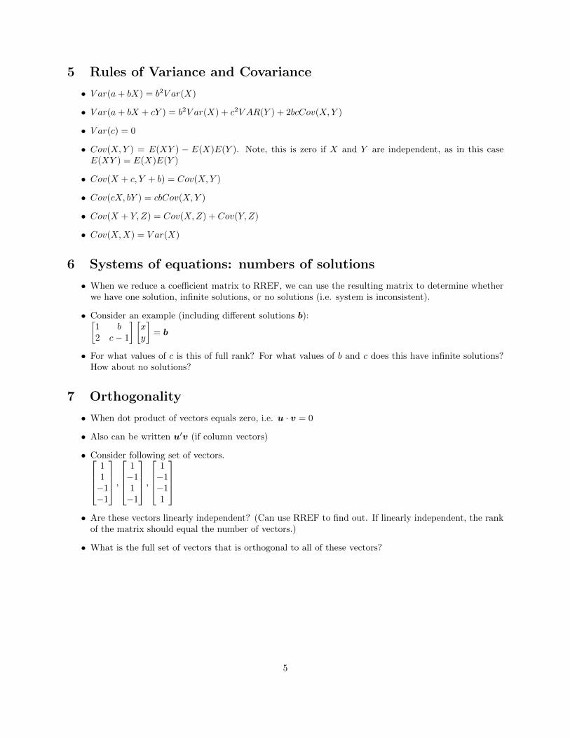
5 Rules of Variance and Covariance

• V ar(a+ bX) = b2V ar(X)

• V ar(a+ bX + cY ) = b2V ar(X) + c2V AR(Y ) + 2bcCov(X,Y )

• V ar(c) = 0

• Cov(X,Y ) = E(XY ) − E(X)E(Y ). Note, this is zero if X and Y are independent, as in this caseE(XY ) = E(X)E(Y )

• Cov(X + c, Y + b) = Cov(X,Y )

• Cov(cX, bY ) = cbCov(X,Y )

• Cov(X + Y,Z) = Cov(X,Z) + Cov(Y,Z)

• Cov(X,X) = V ar(X)

6 Systems of equations: numbers of solutions

• When we reduce a coefficient matrix to RREF, we can use the resulting matrix to determine whetherwe have one solution, infinite solutions, or no solutions (i.e. system is inconsistent).

• Consider an example (including different solutions b):[1 b2 c− 1

] [xy

]= b

• For what values of c is this of full rank? For what values of b and c does this have infinite solutions?How about no solutions?

7 Orthogonality

• When dot product of vectors equals zero, i.e. u · v = 0

• Also can be written u′v (if column vectors)

• Consider following set of vectors.11−1−1

,

1−11−1

,

1−1−11

• Are these vectors linearly independent? (Can use RREF to find out. If linearly independent, the rank

of the matrix should equal the number of vectors.)

• What is the full set of vectors that is orthogonal to all of these vectors?

5

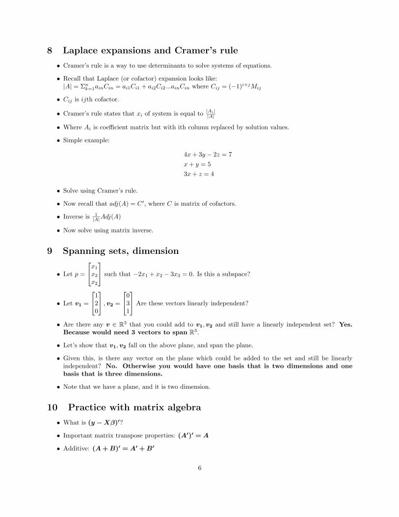
8 Laplace expansions and Cramer’s rule

• Cramer’s rule is a way to use determinants to solve systems of equations.

• Recall that Laplace (or cofactor) expansion looks like:|A| = Σnk=1ainCin = ai1Ci1 + ai2Ci2...ainCin where Cij = (−1)i+jMij

• Cij is ijth cofactor.

• Cramer’s rule states that xi of system is equal to |Ai||A|

• Where Ai is coefficient matrix but with ith column replaced by solution values.

• Simple example:

4x+ 3y − 2z = 7

x+ y = 5

3x+ z = 4

• Solve using Cramer’s rule.

• Now recall that adj(A) = C ′, where C is matrix of cofactors.

• Inverse is 1|A|Adj(A)

• Now solve using matrix inverse.

9 Spanning sets, dimension

• Let p =

x1x2x2

such that −2x1 + x2 − 3x3 = 0. Is this a subspace?

• Let v1 =

120

,v2 =

031

Are these vectors linearly independent?

• Are there any v ∈ R3 that you could add to v1,v2 and still have a linearly independent set? Yes.Because would need 3 vectors to span R3.

• Let’s show that v1,v2 fall on the above plane, and span the plane.

• Given this, is there any vector on the plane which could be added to the set and still be linearlyindependent? No. Otherwise you would have one basis that is two dimensions and onebasis that is three dimensions.

• Note that we have a plane, and it is two dimension.

10 Practice with matrix algebra

• What is (y−Xβ)′?

• Important matrix transpose properties: (A′)′ = A

• Additive: (A+B)′ = A′ +B′

6

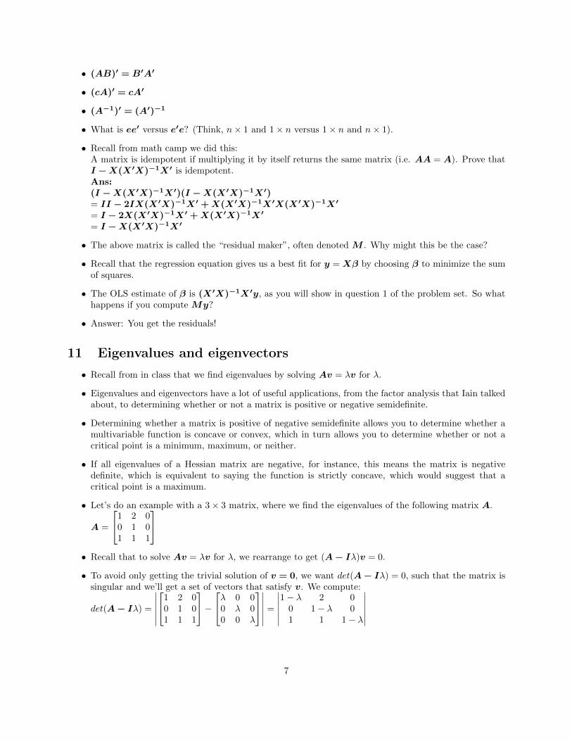
• (AB)′ = B′A′

• (cA)′ = cA′

• (A−1)′ = (A′)−1

• What is ee′ versus e′e? (Think, n× 1 and 1× n versus 1× n and n× 1).

• Recall from math camp we did this:A matrix is idempotent if multiplying it by itself returns the same matrix (i.e. AA = A). Prove thatI −X(X′X)−1X′ is idempotent.Ans:(I −X(X′X)−1X′)(I −X(X′X)−1X′)= II − 2IX(X′X)−1X′ +X(X′X)−1X′X(X′X)−1X′

= I − 2X(X′X)−1X′ +X(X′X)−1X′

= I −X(X′X)−1X′

• The above matrix is called the “residual maker”, often denoted M . Why might this be the case?

• Recall that the regression equation gives us a best fit for y = Xβ by choosing β to minimize the sumof squares.

• The OLS estimate of β is (X′X)−1X′y, as you will show in question 1 of the problem set. So whathappens if you compute My?

• Answer: You get the residuals!

11 Eigenvalues and eigenvectors

• Recall from in class that we find eigenvalues by solving Av = λv for λ.

• Eigenvalues and eigenvectors have a lot of useful applications, from the factor analysis that Iain talkedabout, to determining whether or not a matrix is positive or negative semidefinite.

• Determining whether a matrix is positive of negative semidefinite allows you to determine whether amultivariable function is concave or convex, which in turn allows you to determine whether or not acritical point is a minimum, maximum, or neither.

• If all eigenvalues of a Hessian matrix are negative, for instance, this means the matrix is negativedefinite, which is equivalent to saying the function is strictly concave, which would suggest that acritical point is a maximum.

• Let’s do an example with a 3× 3 matrix, where we find the eigenvalues of the following matrix A.

A =

1 2 00 1 01 1 1

• Recall that to solve Av = λv for λ, we rearrange to get (A− Iλ)v = 0.

• To avoid only getting the trivial solution of v = 0, we want det(A− Iλ) = 0, such that the matrix issingular and we’ll get a set of vectors that satisfy v. We compute:

det(A− Iλ) =

∣∣∣∣∣∣1 2 0

0 1 01 1 1

−λ 0 0

0 λ 00 0 λ

∣∣∣∣∣∣ =

∣∣∣∣∣∣1− λ 2 0

0 1− λ 01 1 1− λ

∣∣∣∣∣∣

7

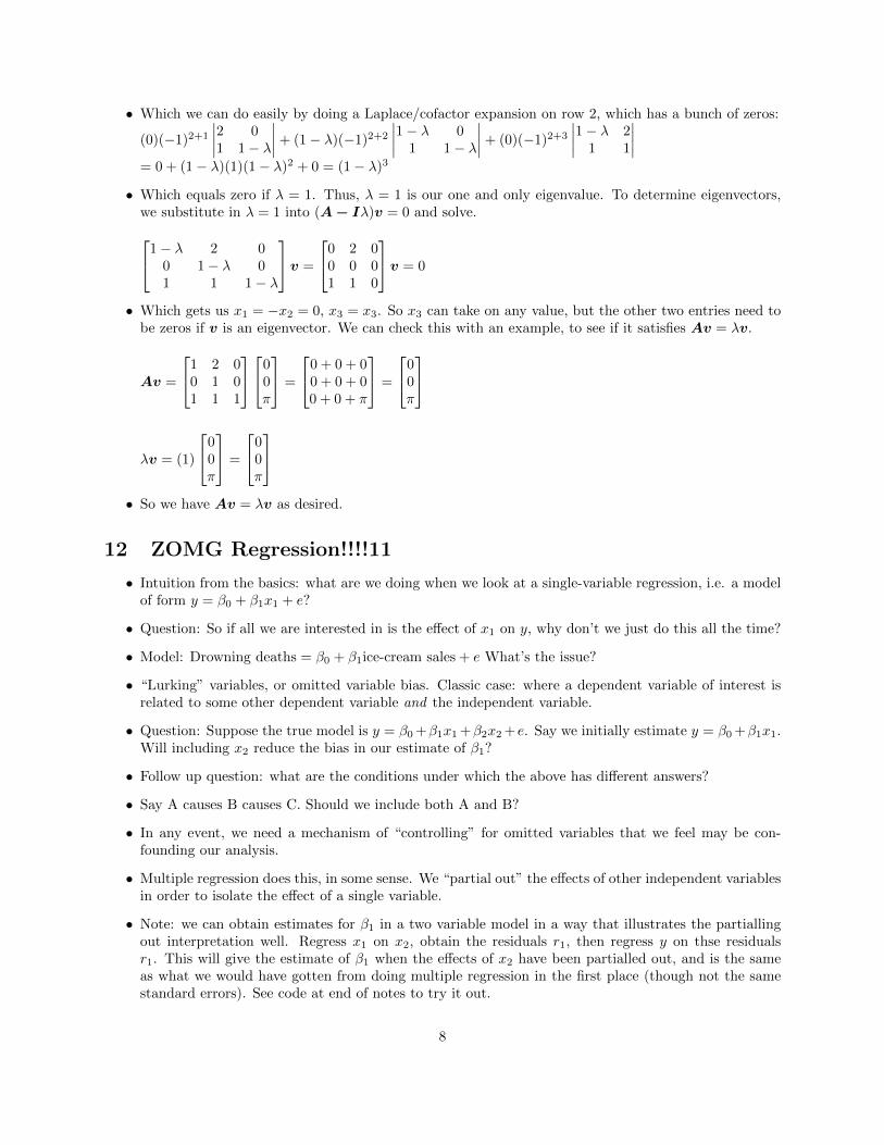
• Which we can do easily by doing a Laplace/cofactor expansion on row 2, which has a bunch of zeros:

(0)(−1)2+1

∣∣∣∣2 01 1− λ

∣∣∣∣+ (1− λ)(−1)2+2

∣∣∣∣1− λ 01 1− λ

∣∣∣∣+ (0)(−1)2+3

∣∣∣∣1− λ 21 1

∣∣∣∣= 0 + (1− λ)(1)(1− λ)2 + 0 = (1− λ)3

• Which equals zero if λ = 1. Thus, λ = 1 is our one and only eigenvalue. To determine eigenvectors,we substitute in λ = 1 into (A− Iλ)v = 0 and solve.1− λ 2 0

0 1− λ 01 1 1− λ

v =

0 2 00 0 01 1 0

v = 0

• Which gets us x1 = −x2 = 0, x3 = x3. So x3 can take on any value, but the other two entries need tobe zeros if v is an eigenvector. We can check this with an example, to see if it satisfies Av = λv.

Av =

1 2 00 1 01 1 1

00π

=

0 + 0 + 00 + 0 + 00 + 0 + π

=

00π

λv = (1)

00π

=

00π

• So we have Av = λv as desired.

12 ZOMG Regression!!!!11

• Intuition from the basics: what are we doing when we look at a single-variable regression, i.e. a modelof form y = β0 + β1x1 + e?

• Question: So if all we are interested in is the effect of x1 on y, why don’t we just do this all the time?

• Model: Drowning deaths = β0 + β1ice-cream sales + e What’s the issue?

• “Lurking” variables, or omitted variable bias. Classic case: where a dependent variable of interest isrelated to some other dependent variable and the independent variable.

• Question: Suppose the true model is y = β0 +β1x1 +β2x2 +e. Say we initially estimate y = β0 +β1x1.Will including x2 reduce the bias in our estimate of β1?

• Follow up question: what are the conditions under which the above has different answers?

• Say A causes B causes C. Should we include both A and B?

• In any event, we need a mechanism of “controlling” for omitted variables that we feel may be con-founding our analysis.

• Multiple regression does this, in some sense. We “partial out” the effects of other independent variablesin order to isolate the effect of a single variable.

• Note: we can obtain estimates for β1 in a two variable model in a way that illustrates the partiallingout interpretation well. Regress x1 on x2, obtain the residuals r1, then regress y on thse residualsr1. This will give the estimate of β1 when the effects of x2 have been partialled out, and is the sameas what we would have gotten from doing multiple regression in the first place (though not the samestandard errors). See code at end of notes to try it out.

8

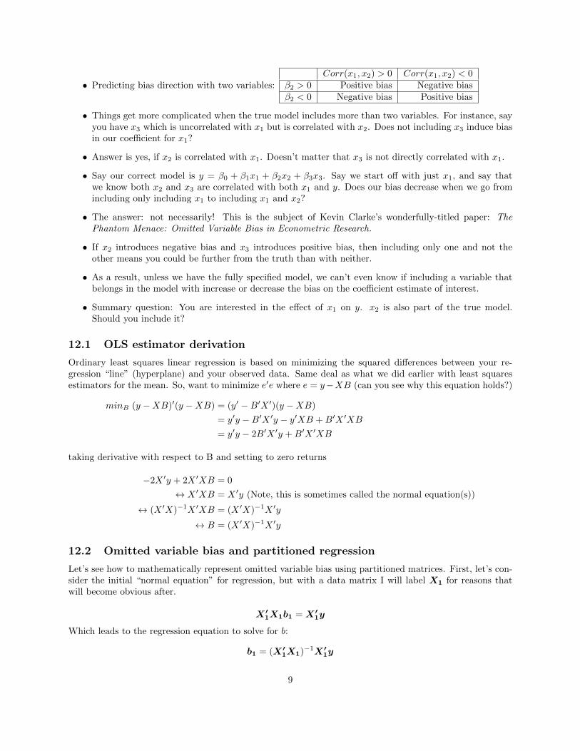
• Predicting bias direction with two variables:Corr(x1, x2) > 0 Corr(x1, x2) < 0

β2 > 0 Positive bias Negative biasβ2 < 0 Negative bias Positive bias

• Things get more complicated when the true model includes more than two variables. For instance, sayyou have x3 which is uncorrelated with x1 but is correlated with x2. Does not including x3 induce biasin our coefficient for x1?

• Answer is yes, if x2 is correlated with x1. Doesn’t matter that x3 is not directly correlated with x1.

• Say our correct model is y = β0 + β1x1 + β2x2 + β3x3. Say we start off with just x1, and say thatwe know both x2 and x3 are correlated with both x1 and y. Does our bias decrease when we go fromincluding only including x1 to including x1 and x2?

• The answer: not necessarily! This is the subject of Kevin Clarke’s wonderfully-titled paper: ThePhantom Menace: Omitted Variable Bias in Econometric Research.

• If x2 introduces negative bias and x3 introduces positive bias, then including only one and not theother means you could be further from the truth than with neither.

• As a result, unless we have the fully specified model, we can’t even know if including a variable thatbelongs in the model with increase or decrease the bias on the coefficient estimate of interest.

• Summary question: You are interested in the effect of x1 on y. x2 is also part of the true model.Should you include it?

12.1 OLS estimator derivation

Ordinary least squares linear regression is based on minimizing the squared differences between your re-gression “line” (hyperplane) and your observed data. Same deal as what we did earlier with least squaresestimators for the mean. So, want to minimize e′e where e = y−XB (can you see why this equation holds?)

minB (y −XB)′(y −XB) = (y′ −B′X ′)(y −XB)

= y′y −B′X ′y − y′XB +B′X ′XB

= y′y − 2B′X ′y +B′X ′XB

taking derivative with respect to B and setting to zero returns

−2X ′y + 2X ′XB = 0

↔ X ′XB = X ′y (Note, this is sometimes called the normal equation(s))

↔ (X ′X)−1X ′XB = (X ′X)−1X ′y

↔ B = (X ′X)−1X ′y

12.2 Omitted variable bias and partitioned regression

Let’s see how to mathematically represent omitted variable bias using partitioned matrices. First, let’s con-sider the initial “normal equation” for regression, but with a data matrix I will label X1 for reasons thatwill become obvious after.

X′1X1b1 = X′1y

Which leads to the regression equation to solve for b:

b1 = (X′1X1)−1X′1y

9

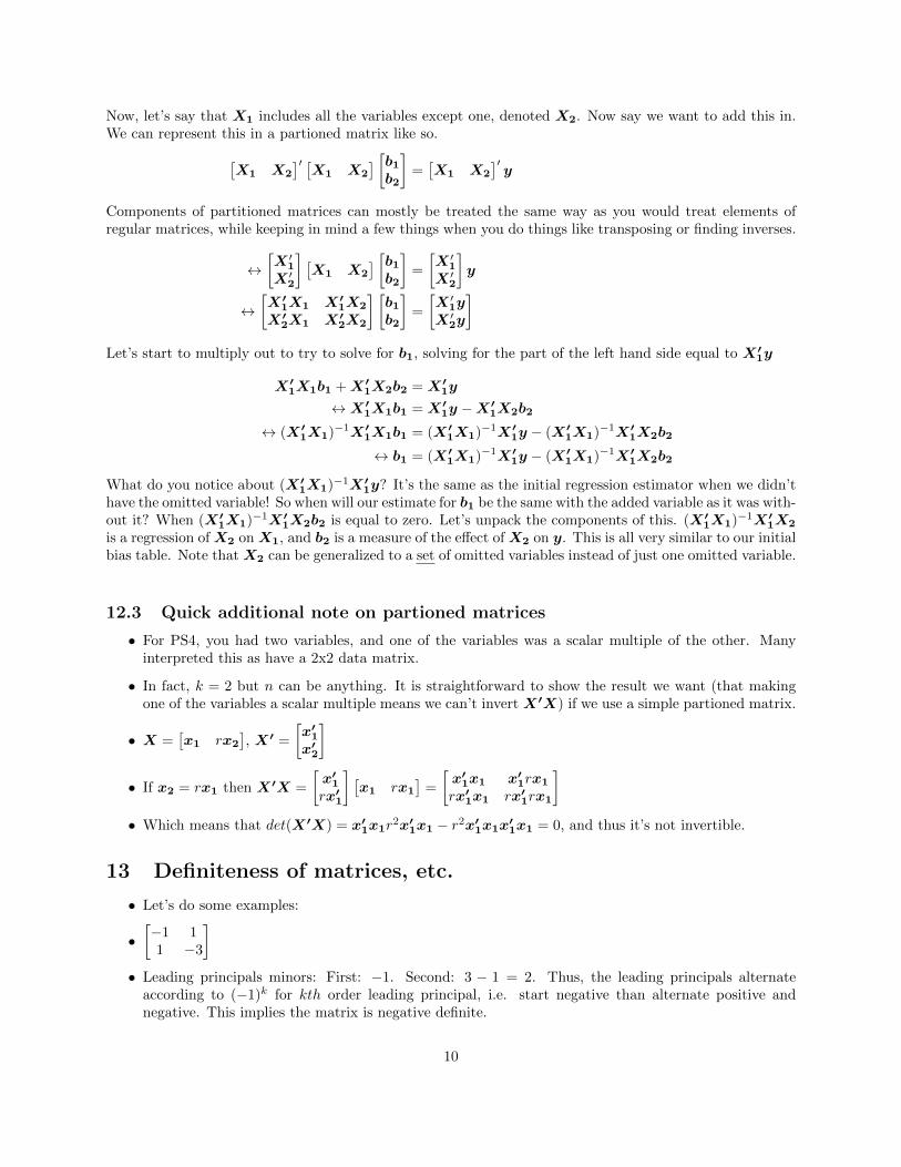
Now, let’s say that X1 includes all the variables except one, denoted X2. Now say we want to add this in.We can represent this in a partioned matrix like so.[

X1 X2

]′ [X1 X2

] [b1b2

]=[X1 X2

]′y

Components of partitioned matrices can mostly be treated the same way as you would treat elements ofregular matrices, while keeping in mind a few things when you do things like transposing or finding inverses.

↔[X ′1X ′2

] [X1 X2

] [b1b2

]=

[X ′1X ′2

]y

↔[X′1X1 X′1X2

X′2X1 X′2X2

] [b1b2

]=

[X ′1yX ′2y

]Let’s start to multiply out to try to solve for b1, solving for the part of the left hand side equal to X′1y

X′1X1b1 +X′1X2b2 = X′1y

↔X′1X1b1 = X′1y −X′1X2b2

↔ (X′1X1)−1X′1X1b1 = (X′1X1)−1X′1y − (X′1X1)−1X′1X2b2

↔ b1 = (X′1X1)−1X′1y − (X′1X1)−1X′1X2b2

What do you notice about (X′1X1)−1X′1y? It’s the same as the initial regression estimator when we didn’thave the omitted variable! So when will our estimate for b1 be the same with the added variable as it was with-out it? When (X′1X1)−1X′1X2b2 is equal to zero. Let’s unpack the components of this. (X′1X1)−1X′1X2

is a regression of X2 on X1, and b2 is a measure of the effect of X2 on y. This is all very similar to our initialbias table. Note that X2 can be generalized to a set of omitted variables instead of just one omitted variable.

12.3 Quick additional note on partioned matrices

• For PS4, you had two variables, and one of the variables was a scalar multiple of the other. Manyinterpreted this as have a 2x2 data matrix.

• In fact, k = 2 but n can be anything. It is straightforward to show the result we want (that makingone of the variables a scalar multiple means we can’t invert X′X) if we use a simple partioned matrix.

• X =[x1 rx2

], X′ =

[x′1x′2

]• If x2 = rx1 then X′X =

[x′1rx′1

] [x1 rx1

]=

[x′1x1 x′1rx1

rx′1x1 rx′1rx1

]• Which means that det(X′X) = x′1x1r

2x′1x1 − r2x′1x1x′1x1 = 0, and thus it’s not invertible.

13 Definiteness of matrices, etc.

• Let’s do some examples:

•[−1 11 −3

]• Leading principals minors: First: −1. Second: 3 − 1 = 2. Thus, the leading principals alternate

according to (−1)k for kth order leading principal, i.e. start negative than alternate positive andnegative. This implies the matrix is negative definite.

10

•[

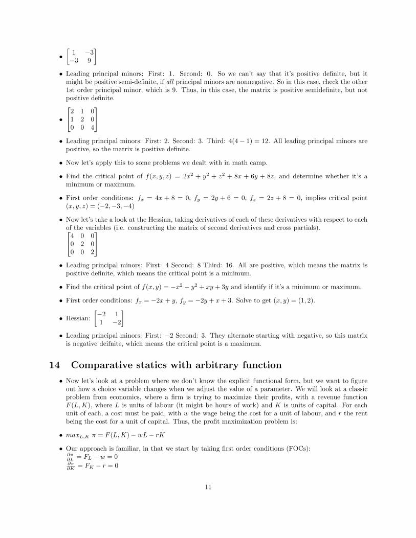
1 −3−3 9

]• Leading principal minors: First: 1. Second: 0. So we can’t say that it’s positive definite, but it

might be positive semi-definite, if all principal minors are nonnegative. So in this case, check the other1st order principal minor, which is 9. Thus, in this case, the matrix is positive semidefinite, but notpositive definite.

•

2 1 01 2 00 0 4

• Leading principal minors: First: 2. Second: 3. Third: 4(4− 1) = 12. All leading principal minors are

positive, so the matrix is positive definite.

• Now let’s apply this to some problems we dealt with in math camp.

• Find the critical point of f(x, y, z) = 2x2 + y2 + z2 + 8x + 6y + 8z, and determine whether it’s aminimum or maximum.

• First order conditions: fx = 4x + 8 = 0, fy = 2y + 6 = 0, fz = 2z + 8 = 0, implies critical point(x, y, z) = (−2,−3,−4)

• Now let’s take a look at the Hessian, taking derivatives of each of these derivatives with respect to eachof the variables (i.e. constructing the matrix of second derivatives and cross partials).4 0 0

0 2 00 0 2

• Leading principal minors: First: 4 Second: 8 Third: 16. All are positive, which means the matrix is

positive definite, which means the critical point is a minimum.

• Find the critical point of f(x, y) = −x2 − y2 + xy + 3y and identify if it’s a minimum or maximum.

• First order conditions: fx = −2x+ y, fy = −2y + x+ 3. Solve to get (x, y) = (1, 2).

• Hessian:

[−2 11 −2

]• Leading principal minors: First: −2 Second: 3. They alternate starting with negative, so this matrix

is negative deifnite, which means the critical point is a maximum.

14 Comparative statics with arbitrary function

• Now let’s look at a problem where we don’t know the explicit functional form, but we want to figureout how a choice variable changes when we adjust the value of a parameter. We will look at a classicproblem from economics, where a firm is trying to maximize their profits, with a revenue functionF (L,K), where L is units of labour (it might be hours of work) and K is units of capital. For eachunit of each, a cost must be paid, with w the wage being the cost for a unit of labour, and r the rentbeing the cost for a unit of capital. Thus, the profit maximization problem is:

• maxL,K π = F (L,K)− wL− rK

• Our approach is familiar, in that we start by taking first order conditions (FOCs):∂π∂L = FL − w = 0∂π∂K = FK − r = 0

11

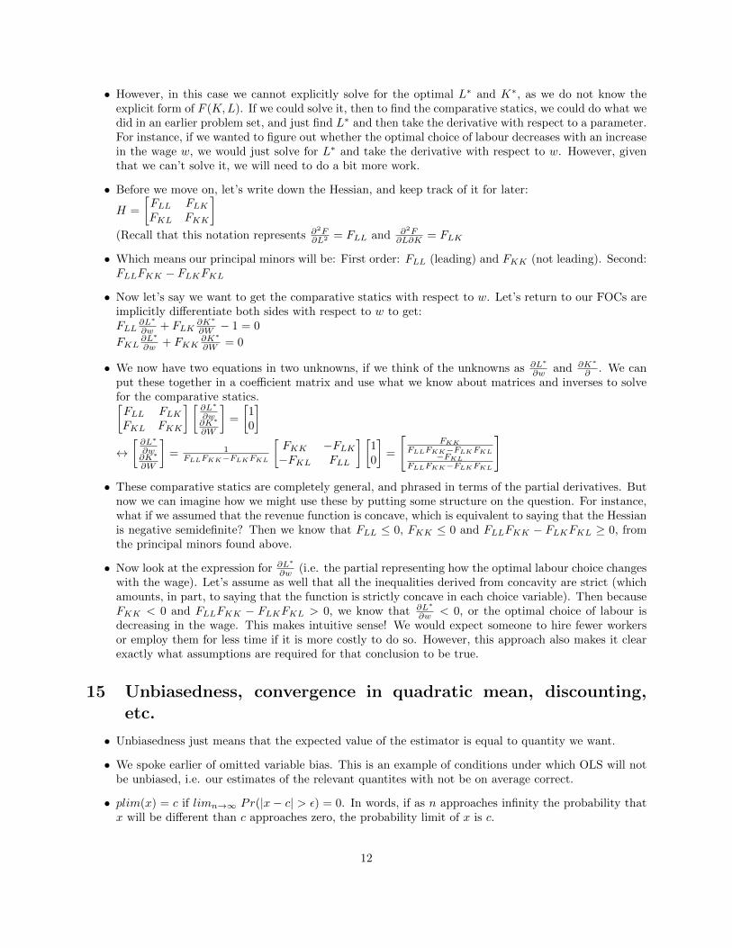
• However, in this case we cannot explicitly solve for the optimal L∗ and K∗, as we do not know theexplicit form of F (K,L). If we could solve it, then to find the comparative statics, we could do what wedid in an earlier problem set, and just find L∗ and then take the derivative with respect to a parameter.For instance, if we wanted to figure out whether the optimal choice of labour decreases with an increasein the wage w, we would just solve for L∗ and take the derivative with respect to w. However, giventhat we can’t solve it, we will need to do a bit more work.

• Before we move on, let’s write down the Hessian, and keep track of it for later:

H =

[FLL FLKFKL FKK

](Recall that this notation represents ∂2F

∂L2 = FLL and ∂2F∂L∂K = FLK

• Which means our principal minors will be: First order: FLL (leading) and FKK (not leading). Second:FLLFKK − FLKFKL

• Now let’s say we want to get the comparative statics with respect to w. Let’s return to our FOCs areimplicitly differentiate both sides with respect to w to get:FLL

∂L∗

∂w + FLK∂K∗

∂W − 1 = 0

FKL∂L∗

∂w + FKK∂K∗

∂W = 0

• We now have two equations in two unknowns, if we think of the unknowns as ∂L∗

∂w and ∂K∗

∂ . We canput these together in a coefficient matrix and use what we know about matrices and inverses to solvefor the comparative statics.[FLL FLKFKL FKK

] [∂L∗

∂w∂K∗

∂W

]=

[10

]↔[∂L∗

∂w∂K∗

∂W

]= 1

FLLFKK−FLKFKL

[FKK −FLK−FKL FLL

] [10

]=

[FKK

FLLFKK−FLKFKL−FKL

FLLFKK−FLKFKL

]• These comparative statics are completely general, and phrased in terms of the partial derivatives. But

now we can imagine how we might use these by putting some structure on the question. For instance,what if we assumed that the revenue function is concave, which is equivalent to saying that the Hessianis negative semidefinite? Then we know that FLL ≤ 0, FKK ≤ 0 and FLLFKK − FLKFKL ≥ 0, fromthe principal minors found above.

• Now look at the expression for ∂L∗

∂w (i.e. the partial representing how the optimal labour choice changeswith the wage). Let’s assume as well that all the inequalities derived from concavity are strict (whichamounts, in part, to saying that the function is strictly concave in each choice variable). Then becauseFKK < 0 and FLLFKK − FLKFKL > 0, we know that ∂L∗

∂w < 0, or the optimal choice of labour isdecreasing in the wage. This makes intuitive sense! We would expect someone to hire fewer workersor employ them for less time if it is more costly to do so. However, this approach also makes it clearexactly what assumptions are required for that conclusion to be true.

15 Unbiasedness, convergence in quadratic mean, discounting,etc.

• Unbiasedness just means that the expected value of the estimator is equal to quantity we want.

• We spoke earlier of omitted variable bias. This is an example of conditions under which OLS will notbe unbiased, i.e. our estimates of the relevant quantites with not be on average correct.

• plim(x) = c if limn→∞ Pr(|x− c| > ε) = 0. In words, if as n approaches infinity the probability thatx will be different than c approaches zero, the probability limit of x is c.

12

• Convergence in quadratic mean requires convergence in the first moment (i.e. the expected value) aswell as the second moment (i.e. the variance). If E(x) converges to c and V ar(x) converges to 0, thenplim(x) = c

• With discounted payoff y over an infinite period of time, you have an infinite geometric series, whichconverges to value y

1−δ for δ ∈ (0, 1). This can be shown using the telescoping series stuff Iain talkedabout, but you can just take it as a given for the problem set (and, most likely, generally in life).

16 Constrained Optimization

• We’ve seen in lecture that equality-constrained optimization can be handled pretty straightforwardlyby constructing the Lagrangian with the constraint added in, and then taking an extra derivative withrespect to λ and solving the new system. From forever ago (math camp) you may recall that I gave asnake fighting problem on a problem set, which is reproduced here:

Now, assume that you derive positive utility from shrinking the size of the snake by workingon your dissertation (think of this as negative negative utility), and that this positive utilityhas decreasing marginal returns in the number of hours per day x you spend working on yourdissertation (completing ANYTHING shrinks the snake a lot, but improvements afterwardshave a higher work to snake-shrinking ratio). This utility will be captured in this problemby 12

√x. Now assume that you could also spend time honing your snake-battling skills,

by practicing snake-fighting, trapping, learning the flute, etc. Denote the time spent onthis as t, and the utility gained from this as 3t (so your utility from snake-battling trainingincreases at a constant rate/does not experience decreasing marginal returns). Now assumethat you have 16 hours a day to allocate between your thesis and snake-fight training, suchthat t = 16− x. Thus, your utility function can be expressed as:

U(x, t) = 12√x+ 3t = U(x) = 12

√x+ 3(16− x)

• You could solve this by just taking a derivative and setting to zero. You might notice, howver, thatthis is essentially an equality-constrained maximization problem! I have built the constraint into theproblem, by making the number of hours spent on snake-fight training 16− x.

• The Lagrange approach intuition has some similarities. This is what Iain means when he says thateach constraint “nails down” a particular variable; in this case, one constraint nails down the y interms of x

• The answer in this case was x = 4 hours on the dissertation and 12 hours spent training to fight snakes.We can get the same answer by setting up the Lagrangian.

• L(x, t, λ) = 12√x+ 3t+ λ(16− x− t)

∂L∂x = 6x−1/2 − λ = 0∂L∂t = 3− λ = 0∂L∂λ = 16− x− t = 0

• Which we can solve, noting that the second expression gives us λ = 3. Which means that 6x−1/2 =3↔ 2 =

√x↔ x = 4. We then plug into the third expression to get t, i.e. 16− 4− t = 0↔ t = 12

• Inequality constraints, and Kuhn-Tucker (KT) conditions, are grosser looking, but are essential just away of formalizing the idea of checking whether or not each constraint is binding or not.

• Sometimes we impose assumptions on the problem to ensure that we know which constraints will bindand which won’t without having the check each case. For instance, if everyone always wants more ofevery good (monotonic preferences) then the budget constraint will bind.

13

• So let’s go back to the snake-fighting problem, make the constraint an inequality one x + t < 16 andadd in another inequality constraint that t > 1. Perhaps you live in a snake-infested area and are likelyto be attacked by snakes for an hour a day irrespective of your choices. We can set up the Lagrangian:L(x, t) = 12

√x+ 3t+ λ1(16− x− t) + λ2(t− 1)

• Where we only take derivatives with respect to variables and binding constraints.∂L∂x = 6x−1/2 − λ1 = 0∂L∂t = 3− λ1 + λ2 = 0

• This gives us 6 Kuhn-Tucker conditions in addition to the original three first order conditions:λ1 ≥ 0, 16− x− t ≥ 0, λ1(16− x− t) = 0λ2 ≥ 0, t− 1 ≥ 0, λ2(t− 1) = 0

• Any points that satisfying the first order conditions and KT conditions are fair game for minima andmaxima. As mentioned earlier, we might be able to rule out certain constraints binding or not bindingbased on how we’ve structured the problem. Failing that, we need to check each condition, which cangive us a number of “cases” that are candidates for solutions. See below:

• Assume t = 1 which implies λ2 ≥ 0. Two possible options: (1) 16− x− 1 = 15− x = 0 and λ1 ≥ 0 or(2) λ1 = 0 and 15− x ≥ 0. Looking at (2), if we then look at the first FOC, we get 6x−1/2 = 0, whichcannot hold for any x, so this is not a candidate. Option (1) gives us x = 15, which with the first FOCgives us approximately λ1 = 1.5. Plugging into the second FOC, we get 3− 1.5 +λ2 = 0↔ λ2 = −1.5,which contradicts the our initial assumption that λ2 ≥ 0. So this is also not a candidate. So we haveruled out t = 1, and can move on to evaluating the converse.

• Assume t − 1 ≥ 0 and λ2 = 0. Two possible options: (1) 16 − x − t = 0 and λ1 ≥ 0 or (2) λ1 = 0and 15 − x ≥ 0. Once again, let’s start with option 2. If λ1 = 0, we have from the second FOC that3− λ1 + λ2 = 3− 0 + 0 = 0, which cannot be true, so this cannot be a candidate. So we are left withonly the last candidate, which is where the constraint 16 − x − t holds with equality. This gives usx = 4, t = 12 as before, and we can check and see that all KT conditions are satisfied.

• Essentially, every KT condition gives us two possible options, which have to be checked against everyother option in the other KT conditions. So we get 2r cases for each r inequality constraints.

• Note, finally, that all of these conditions essentially correspond to assuming a constraint is binding ornot, and then checking the implications for contradictions with the FOCs or the other KT conditions.

17 Game theory

17.1 Nash Equilibrium

• Games consist of a set of N players, S strategies, and U payoffs over strategy profiles (a vectors ofeach player’s strategies).

• Nash equilibrium: All strategies are elements of each player’s best response correspondence, giveneveryone else’s strategies.

• Note that each strategy profile is a candidate for equilibrium, and Nash allows us to restrict ourattention to a subset of strategy profiles.

• Implies: no player has an incentive to deviate from their current strategy, given the other player’sstrategies.

• Formally: s∗ is Nash if ∀i ∈ N, ui(s∗i ) ≥ ui(si, s∗−i),∀si ∈ Si

• (With this notation, “−i” means every player outside of player i)

14

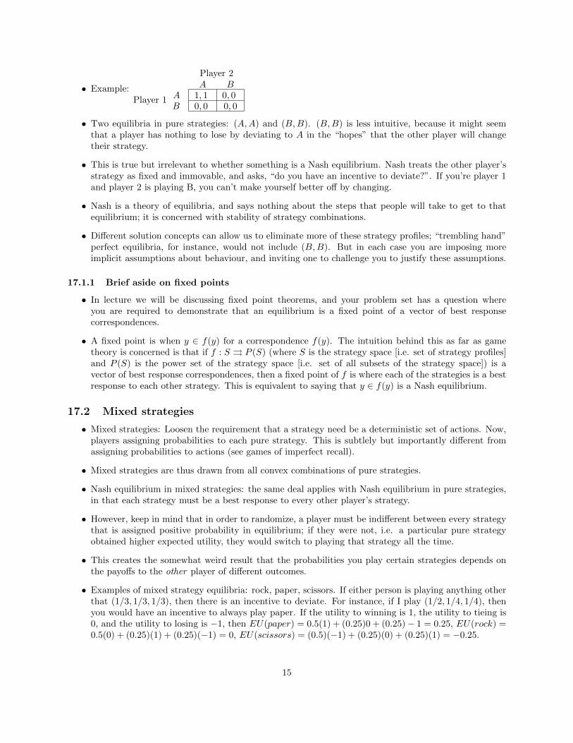
• Example:Player 1

Player 2A B

A 1, 1 0, 0B 0, 0 0, 0

• Two equilibria in pure strategies: (A,A) and (B,B). (B,B) is less intuitive, because it might seemthat a player has nothing to lose by deviating to A in the “hopes” that the other player will changetheir strategy.

• This is true but irrelevant to whether something is a Nash equilibrium. Nash treats the other player’sstrategy as fixed and immovable, and asks, “do you have an incentive to deviate?”. If you’re player 1and player 2 is playing B, you can’t make yourself better off by changing.

• Nash is a theory of equilibria, and says nothing about the steps that people will take to get to thatequilibrium; it is concerned with stability of strategy combinations.

• Different solution concepts can allow us to eliminate more of these strategy profiles; “trembling hand”perfect equilibria, for instance, would not include (B,B). But in each case you are imposing moreimplicit assumptions about behaviour, and inviting one to challenge you to justify these assumptions.

17.1.1 Brief aside on fixed points

• In lecture we will be discussing fixed point theorems, and your problem set has a question whereyou are required to demonstrate that an equilibrium is a fixed point of a vector of best responsecorrespondences.

• A fixed point is when y ∈ f(y) for a correspondence f(y). The intuition behind this as far as gametheory is concerned is that if f : S ⇒ P (S) (where S is the strategy space [i.e. set of strategy profiles]and P (S) is the power set of the strategy space [i.e. set of all subsets of the strategy space]) is avector of best response correspondences, then a fixed point of f is where each of the strategies is a bestresponse to each other strategy. This is equivalent to saying that y ∈ f(y) is a Nash equilibrium.

17.2 Mixed strategies

• Mixed strategies: Loosen the requirement that a strategy need be a deterministic set of actions. Now,players assigning probabilities to each pure strategy. This is subtlely but importantly different fromassigning probabilities to actions (see games of imperfect recall).

• Mixed strategies are thus drawn from all convex combinations of pure strategies.

• Nash equilibrium in mixed strategies: the same deal applies with Nash equilibrium in pure strategies,in that each strategy must be a best response to every other player’s strategy.

• However, keep in mind that in order to randomize, a player must be indifferent between every strategythat is assigned positive probability in equilibrium; if they were not, i.e. a particular pure strategyobtained higher expected utility, they would switch to playing that strategy all the time.

• This creates the somewhat weird result that the probabilities you play certain strategies depends onthe payoffs to the other player of different outcomes.

• Examples of mixed strategy equilibria: rock, paper, scissors. If either person is playing anything otherthat (1/3, 1/3, 1/3), then there is an incentive to deviate. For instance, if I play (1/2, 1/4, 1/4), thenyou would have an incentive to always play paper. If the utility to winning is 1, the utility to tieing is0, and the utility to losing is −1, then EU(paper) = 0.5(1) + (0.25)0 + (0.25)− 1 = 0.25, EU(rock) =0.5(0) + (0.25)(1) + (0.25)(−1) = 0, EU(scissors) = (0.5)(−1) + (0.25)(0) + (0.25)(1) = −0.25.

15

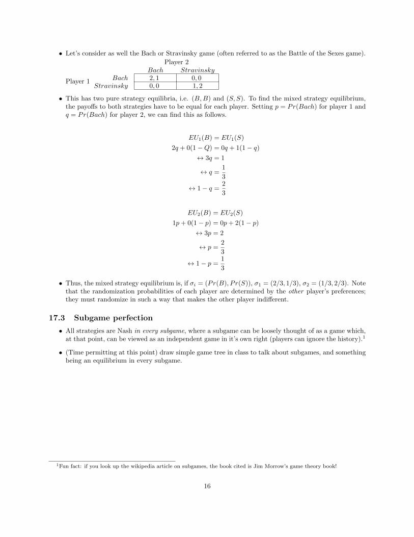
• Let’s consider as well the Bach or Stravinsky game (often referred to as the Battle of the Sexes game).

Player 1

Player 2Bach Stravinsky

Bach 2, 1 0, 0Stravinsky 0, 0 1, 2

• This has two pure strategy equilibria, i.e. (B,B) and (S, S). To find the mixed strategy equilibrium,the payoffs to both strategies have to be equal for each player. Setting p = Pr(Bach) for player 1 andq = Pr(Bach) for player 2, we can find this as follows.

EU1(B) = EU1(S)

2q + 0(1−Q) = 0q + 1(1− q)↔ 3q = 1

↔ q =1

3

↔ 1− q =2

3

EU2(B) = EU2(S)

1p+ 0(1− p) = 0p+ 2(1− p)↔ 3p = 2

↔ p =2

3

↔ 1− p =1

3

• Thus, the mixed strategy equilibrium is, if σi = (Pr(B), P r(S)), σ1 = (2/3, 1/3), σ2 = (1/3, 2/3). Notethat the randomization probabilities of each player are determined by the other player’s preferences;they must randomize in such a way that makes the other player indifferent.

17.3 Subgame perfection

• All strategies are Nash in every subgame, where a subgame can be loosely thought of as a game which,at that point, can be viewed as an independent game in it’s own right (players can ignore the history).1

• (Time permitting at this point) draw simple game tree in class to talk about subgames, and somethingbeing an equilibrium in every subgame.

1Fun fact: if you look up the wikipedia article on subgames, the book cited is Jim Morrow’s game theory book!

16