Embed Size (px)
Citation preview
Wright State University Wright State University
CORE Scholar CORE Scholar
Browse all Theses and Dissertations Theses and Dissertations
2010
Proximity and Thickness Estimation of Aluminum 3003 Alloy Proximity and Thickness Estimation of Aluminum 3003 Alloy
Metal Sheets Using Multi-Frequency Eddy Current Sensor Metal Sheets Using Multi-Frequency Eddy Current Sensor
Sunil S. Kamanalu Wright State University
Follow this and additional works at: https://corescholar.libraries.wright.edu/etd_all
Part of the Physics Commons
Repository Citation Repository Citation Kamanalu, Sunil S., "Proximity and Thickness Estimation of Aluminum 3003 Alloy Metal Sheets Using Multi-Frequency Eddy Current Sensor" (2010). Browse all Theses and Dissertations. 379. https://corescholar.libraries.wright.edu/etd_all/379
This Thesis is brought to you for free and open access by the Theses and Dissertations at CORE Scholar. It has been accepted for inclusion in Browse all Theses and Dissertations by an authorized administrator of CORE Scholar. For more information, please contact [email protected].
PROXIMITY AND THICKNESS ESTIMATION OF ALUMINUM 3003
ALLOY METAL SHEETS USING MULTI-FREQUENCY EDDY
CURRENT SENSOR
A thesis submitted in partial fulfillment of the requirements for the degree of
Master of Science
By
SUNIL SONDEKERE KAMANALU M.S., Wright State University, 2002
B.E., Bangalore University, 1999
2010 Wright State University
WRIGHT STATE UNIVERSITY
SCHOOL OF GRADUATE STUDIES
September 9, 2010
I HEREBY RECOMMEND THAT THE THESIS PREPARED UNDER MY
SUPERVISION BY SUNIL SONDEKERE KAMANALU ENTITLED PROXIMITY
AND THICKNESS ESTIMATION OF ALUMINUM 3003 ALLOY METAL SHEETS
USING MULTI-FREQUENCY EDDY CURRENT SENSOR BE ACCEPTED IN
PARTIAL FULFILLMENT OF THE REQUIREMENTS FOR THE DEGREE OF
Master of Science.
Douglas T. Petkie, Ph.D. Thesis Director
Lok C. Lew Yan Voon, Ph.D.
Department Chair Committee on Final Examination Douglas T. Petkie, Ph.D. Jerry D. Clark, Ph.D. Jason A. Deibel, Ph.D. Andrew Toming Hsu, Ph.D. Dean, School of Graduate Studies
ABSTRACT Kamanalu, Sunil Sondekere. M.S., Department of Physics, Wright State University, 2010. Proximity and Thickness Estimation of Aluminum 3003 Alloy Metal Sheets Using Multi-Frequency Eddy Current Sensor.
The research work is focused on conducting a feasibility study on a new “non-
contact” single probe dual coil inductive sensor for sensing the proximity and thickness
of Aluminum (Al) 3003 alloy metal sheets, which is a non-magnetic metal. A bulk of the
research and development (R&D) work has already been done in the area of non-
destructive testing (NDT) using eddy current technology targeted to various applications
like corrosion detection, material thickness, material conductivity, etc. The research work
presented in this thesis uses the prior R&D work completed in NDT as a platform for
conducting this study to estimate proximity and thickness of Aluminum 3003 alloy metal
sheets, which is not considered a flaw detection application. Some of the current
technologies in the area of eddy current NDT for proximity and thickness estimation,
each with its own limitations, include single probe ‘contact’ sensors for magnetic metals,
single probe ‘non-contact’ sensors with separation distance of less than 1 mm and dual
probe sensors that requires probes on both sides of the metal sheet.
A swept multi-frequency scanning technique is used together with an automated
data collection system to measure and collect output voltage and phase difference data
over a wide range of frequencies. The skin effect in conductors and its associated property
of skin depth is used to extract proximity and thickness information from the data
collected, and then correlated with reference values to validate the results. Experimental
iii
iv
results show the output voltage and phase difference of the sensor is dependent on the
metal parameters (resistivity ‘ρ’, permeability ‘μ’, thickness ‘T’) and coil parameters
(diameter ‘D’, frequency ‘F’, lift-off ‘L’). Further, proximity is estimated from output
voltage difference, and metal thickness (single/double) is estimated from phase difference
independent of lift-off, which is a novel approach for thickness detection. The test sensor
provides an accurate measure of proximity and thickness of Al 3003 alloy from a single
sided measurement with varying lift-off, overcoming the limitations of other sensor
configurations.
TABLE OF CONTENTS
ABSTRACT ...................................................................................................................... iii
LIST OF FIGURES ........................................................................................................ vii
LIST OF TABLES ............................................................................................................ x
ACKNOWLEDGEMENT ............................................................................................... xi
DEDICATION................................................................................................................. xii
1 Introduction ................................................................................................................... 1
1.1 Physical Concepts of Eddy Current Testing ....................................................... 3
1.2 Operating Variables ............................................................................................ 5
1.3 Principles of Operation ....................................................................................... 8
1.4 Previous Eddy Current NDT Research Work ..................................................... 9
1.5 Thesis Layout .................................................................................................... 11
2 Mathematical Background ......................................................................................... 12
2.1 Maxwell’s Equations ........................................................................................ 12
2.2 Electric and Magnetic Field Waves in Conductors ........................................... 13
2.3 Skin Depth ........................................................................................................ 15
3 Coil Design and Characterization ............................................................................. 20
3.1 Eddy Current Sensor Components .................................................................... 20
3.2 Coil Specifications ........................................................................................... 21
3.3 Mode of Operation ........................................................................................... 23
3.4 Core Type......................................................................................................... 23
3.5 Coil Configuration ............................................................................................ 24
3.6 Probe Shielding and Loading ........................................................................... 25
v
3.7 Coil Characterization ....................................................................................... 26
4 Experimental Setup and Data Acquisition ............................................................... 30
4.1 Block Diagram .................................................................................................. 30
4.1.1 Waveform Generator ................................................................................ 31
4.1.2 Positioning Slides...................................................................................... 31
4.1.3 Bridge Circuit............................................................................................ 32
4.1.4 Signal Conditioning .................................................................................. 34
4.1.5 Data Acquisition Card ............................................................................... 34
4.1.6 Data Acquisition Flow Chart .................................................................... 36
4.1.7 Feature Extraction & Characterization Algorithms .................................. 38
4.1.8 Data Processing, Analysis & Results ........................................................ 40
5 Results .......................................................................................................................... 42
5.1 Proximity Estimation using Output Voltage ..................................................... 42
5.2 Thickness (Single/Double) Estimation using Phase ......................................... 59
6 Conclusion ................................................................................................................... 69
6.1 Thickness (Single/Double) Estimation ............................................................. 69
6.2 Proximity Estimation ........................................................................................ 73
6.3 Future Work ....................................................................................................... 74
References ........................................................................................................................ 76
Appendix A - Al 3003 Alloy Types ................................................................................ 79
Appendix B - Visual Basic Code for Phase Difference ................................................ 81
vi
LIST OF FIGURES
Figure 1. Eddy currents in a conductive material. .............................................................. 3
Figure 2. Electromagnetic induction process in a coil. ...................................................... 4
Figure 3. Skin depth in a good conductor........................................................................... 7
Figure 4. Depth of penetration. ......................................................................................... 16
Figure 5. Exponential decay of electric and magnetic fields in a conductor. ................... 17
Figure 6. Skin Depth (in.) vs. Frequency (Hz) of Various Aluminum 3003 Alloys. ....... 19
Figure 7. Geometry and dimensions of the air-core coils used in the experiment. .......... 21
Figure 8. Front and side views of the experimental single probe dual coil test sensor. ... 24
Figure 9. Coil model ‘A’ characterization for frequency, F = 0 Hz – 10 KHz. ............... 28
Figure 10. Coil model ‘A’ characterization for frequency, F = 0 Hz – 25 KHz. ............. 28
Figure 11. Coil model ‘A’ characterization for frequency, F = 0 Hz – 50 KHz. ............. 29
Figure 12. Block diagram of experimental setup. ............................................................ 30
Figure 13. Wheatstone bridge circuit and preamplifier. ................................................... 32
Figure 14. Data acquisition flow chart. ............................................................................ 37
Figure 15. Amplitude algorithm. ...................................................................................... 38
Figure 16. Phase algorithm. .............................................................................................. 39
Figure 17. Output voltage vs. Frequency for T = 0.016”. ................................................ 44
Figure 18. Output voltage difference vs. Frequency for T = 0.016”. ............................... 44
Figure 19. Output voltage vs. Frequency for T = 0.020”. ................................................ 45
Figure 20. Output voltage difference vs. Frequency for T = 0.020”. ............................... 46
Figure 21. Output voltage vs. Frequency for T = 0.025”. ................................................ 46
Figure 22. Output voltage difference vs. Frequency for T = 0.025”. ............................... 47
vii
Figure 23. Output voltage vs. Frequency for T = 0.032”. ................................................ 48
Figure 24. Output voltage difference vs. Frequency for T = 0.032”. ............................... 48
Figure 25. Output voltage vs. Frequency for T = 0.040”. ................................................ 49
Figure 26. Output voltage difference vs. Frequency for T = 0.040”. ............................... 50
Figure 27. Output voltage vs. Frequency for T = 0.050”. ............................................... 51
Figure 28. Output voltage difference vs. Frequency for T = 0.050”. ............................... 51
Figure 29. Output voltage vs. Frequency for T = 0.063”. ................................................ 52
Figure 30. Output voltage difference vs. Frequency for T = 0.063”. ............................... 53
Figure 31. Output voltage vs. Frequency for T = 0.080”. ................................................ 53
Figure 32. Output voltage difference vs. Frequency for T = 0.080”. ............................... 54
Figure 33. Output voltage vs. Frequency for T = 0.090”. ................................................ 55
Figure 34. Output voltage difference vs. Frequency for T = 0.090”. ............................... 55
Figure 35. Output voltage vs. Frequency for T = 0.100”. ................................................ 56
Figure 36. Output voltage difference vs. Frequency for T = 0.100”. ............................... 57
Figure 37. Phase vs. Frequency for Lift-off = 0.0”. ......................................................... 60
Figure 38. Phase difference vs. Frequency for Lift-off = 0.0”. ........................................ 61
Figure 39. Phase vs. Frequency for Lift-off = 0.1”. ......................................................... 62
Figure 40. Phase difference vs. Frequency for Lift-off = 0.1”. ........................................ 63
Figure 41. Phase vs. Frequency for Lift-off = 0.2”. ......................................................... 63
Figure 42. Phase difference vs. Frequency for Lift-off = 0.2”. ........................................ 64
Figure 43. Phase vs. Frequency for Lift-off = 0.3”. ......................................................... 64
Figure 44. Phase difference vs. Frequency for Lift-off = 0.3”. ........................................ 65
Figure 45. Phase vs. Frequency for Lift-off = 0.4”. ......................................................... 65
viii
Figure 46. Phase difference vs. Frequency for Lift-off = 0.4”. ........................................ 66
Figure 47. Phase vs. Frequency for Lift-off = 0.5”. ......................................................... 66
Figure 48. Phase difference vs. Frequency for Lift-off = 0.5”. ........................................ 67
Figure 49. Phase vs. Frequency for Lift-off = 0.6”. ......................................................... 67
Figure 50. Phase difference vs. Frequency for Lift-off = 0.6”. ........................................ 68
Figure 51. Thickness (single/double) estimation at F = 1 KHz. ....................................... 69
Figure 52. Thickness (single/double) estimation at F = 1.5 KHz. .................................... 70
Figure 53. Thickness (single/double) estimation at F = 2 KHz. ....................................... 71
Figure 54. Average theoretical skin depth for F = 1 KHz, 1.5 KHz, 2 KHz. ................... 72
Figure 55. Proximity estimation at F = 5.5 KHz. ............................................................. 73
ix

LIST OF TABLES
Table 1. Coil specifications. .............................................................................................. 22
Table 2. Coil characterization results. ............................................................................... 27
Table 3. Sampling rates..................................................................................................... 35
Table 4. Maximum output voltage difference for metal sample thicknesses. .................. 58
Table 5. Spread of phase difference between single & double ......................................... 68
Table 6. Aluminum 3003 alloy metal composition. ......................................................... 79
Table 7. Conductivity & resistivity of aluminum 3003 alloy types. ................................. 79
Table 8. Temper designation. ............................................................................................ 80
Table 9. Degree of hardness. ............................................................................................. 80
x
ACKNOWLEDGEMENT
I would like to take this opportunity to express my gratitude and appreciation to
my thesis advisor Dr. Douglas T. Petkie for his advise, encouragement and support
during my entire Master’s program. Further, the ‘Sensors Design’ course offered by Dr.
Petkie was the primary source for my interest and motivation in the field of Sensors.
Special thanks to Dr. Gust Bambakidis, Professor Emeritus, for giving me the
opportunity to pursue my Master’s program.
xi

xii
DEDICATION
I would like to dedicate this thesis in memory of my paternal grandfather Mr. S.
K. Hanumantha Reddy and my maternal grandfather Mr. C. P. Narasimhulu. I would also
like to thank my wife Shilpa, daughter Saanvi, and my family for all the encouragement
and support provided to me in completing my thesis work.

Chapter 1
Introduction
This chapter presents an overview on the theory and underlying principles of eddy
current testing, which is the technique employed in this project for sensing the proximity
and thickness of metal sheets. The objective of this thesis is to conduct a feasibility study
on a new “non-contact” single probe dual coil inductive sensor for sensing the influence
of metal proximity and thickness upon the impedance characteristics of the sensor using a
swept multi-frequency technique and the concept of skin effect in conductors. The
research work presented in this thesis aims to meet the challenges of the metal forming
industry by ensuring that only a single sheet of a specific thickness enters the forming
machine while making the measurement independent of lift-off distance, as their
applications require preserving the integrity of the metal sample and/or space constraint
(machines on which the sensors are installed).
The disadvantages of the current eddy current sensors for such an application are
as follows:
(1) The single probe contact based sensor must make contact with the metal sheet
under test. The probe is used to detect magnetic metals like steel, tinplate,
stainless steel (magnetic).
(2) The single probe non-contact based sensor has limited lift-off capability and must
be placed at a fixed distance of less than 1 mm from the metal sample.
1
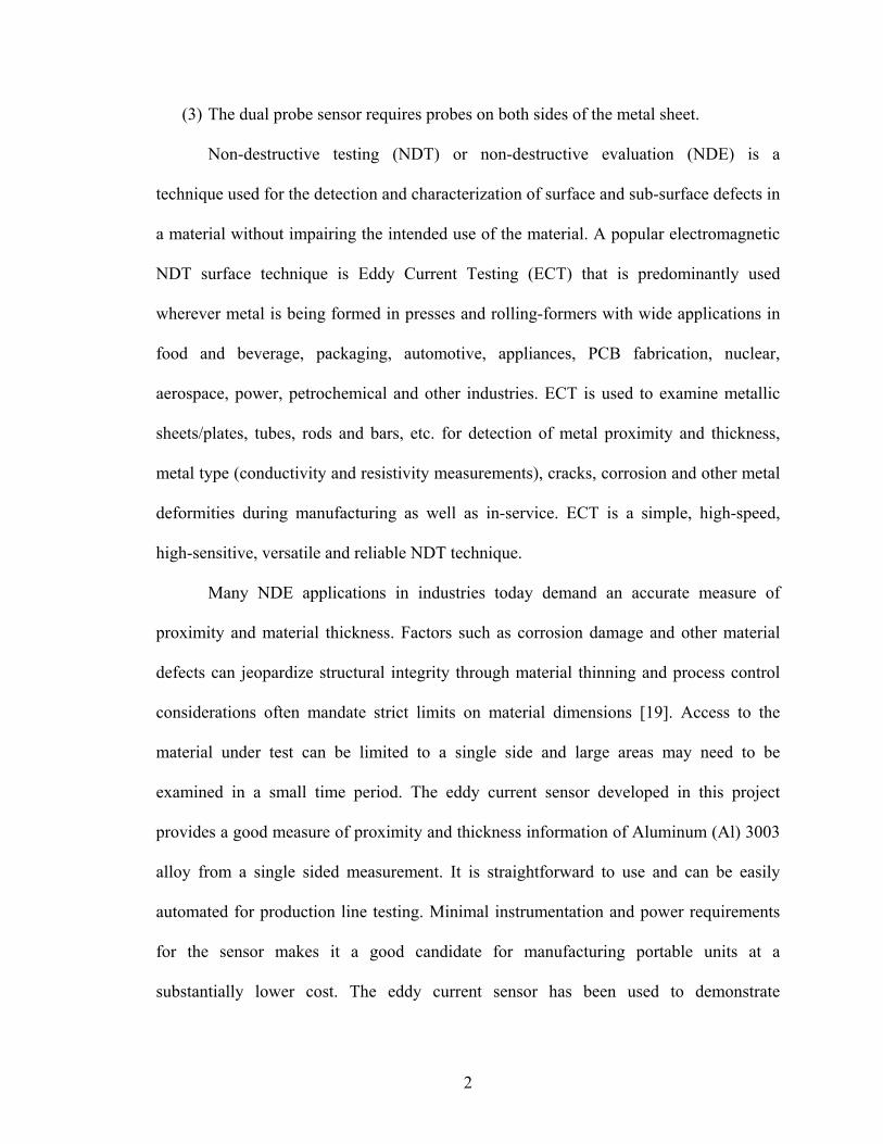
(3) The dual probe sensor requires probes on both sides of the metal sheet.
Non-destructive testing (NDT) or non-destructive evaluation (NDE) is a
technique used for the detection and characterization of surface and sub-surface defects in
a material without impairing the intended use of the material. A popular electromagnetic
NDT surface technique is Eddy Current Testing (ECT) that is predominantly used
wherever metal is being formed in presses and rolling-formers with wide applications in
food and beverage, packaging, automotive, appliances, PCB fabrication, nuclear,
aerospace, power, petrochemical and other industries. ECT is used to examine metallic
sheets/plates, tubes, rods and bars, etc. for detection of metal proximity and thickness,
metal type (conductivity and resistivity measurements), cracks, corrosion and other metal
deformities during manufacturing as well as in-service. ECT is a simple, high-speed,
high-sensitive, versatile and reliable NDT technique.
Many NDE applications in industries today demand an accurate measure of
proximity and material thickness. Factors such as corrosion damage and other material
defects can jeopardize structural integrity through material thinning and process control
considerations often mandate strict limits on material dimensions [19]. Access to the
material under test can be limited to a single side and large areas may need to be
examined in a small time period. The eddy current sensor developed in this project
provides a good measure of proximity and thickness information of Aluminum (Al) 3003
alloy from a single sided measurement. It is straightforward to use and can be easily
automated for production line testing. Minimal instrumentation and power requirements
for the sensor makes it a good candidate for manufacturing portable units at a
substantially lower cost. The eddy current sensor has been used to demonstrate
2
measurement of proximity and thickness of Aluminum 3003 alloy sheets with a
separation (lift-off) distance ranging from 0.0” (probe flush on the metal sheet) to 0.6” in
increments of 0.1”, at a frequency range of 500 Hz to 6 KHz in increments of 500 Hz,
and for the following standard metal thicknesses (single and double): 0.016”, 0.020”,
0.025”, 0.032”, 0.040”, 0.050”, 0.063”, 0.080”, 0.090”, 0.100”. This research work will
explain the output voltage dependence of the sensor as a function of proximity and phase
difference as a function of metal thickness independent of lift-off, which is a novel
approach for thickness detection, and present experimental results for proximity and
thickness gauging. Thickness is defined as a ‘single’, which defines one metal sheet of a
given thickness or a ‘double’, which defines two stacked metal sheets of identical
thickness.
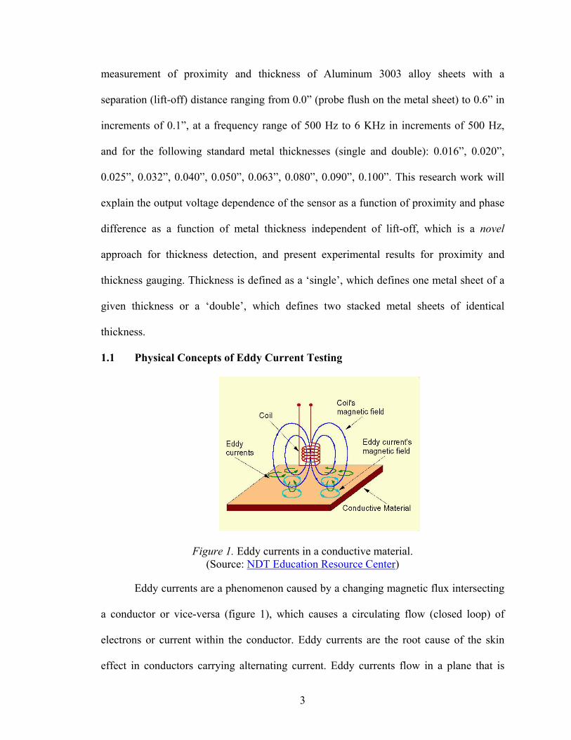
1.1 Physical Concepts of Eddy Current Testing
Figure 1. Eddy currents in a conductive material. (Source: NDT Education Resource Center)
Eddy currents are a phenomenon caused by a changing magnetic flux intersecting
a conductor or vice-versa (figure 1), which causes a circulating flow (closed loop) of
electrons or current within the conductor. Eddy currents are the root cause of the skin
effect in conductors carrying alternating current. Eddy currents flow in a plane that is
3
parallel to the coil winding or material surface and are attenuated and lag in phase with
depth. Eddy current inspection works on the principles of electromagnetic induction. In
ECT, the coil (also called sensor or probe) is excited with a sinusoidal input voltage
source to induce eddy currents in the electrically conducting material under test. Any
regions of metal discontinuities or deformities cause an impedance change in the sensing
coil, and the resultant differential impedance between the reference and sensing coils is
measured and correlated with the corresponding defect. Eddy currents are not uniformly
distributed throughout a material being inspected; rather they are densest at the surface
immediately beneath the coil and exhibit an exponential decay with increasing distance
below the surface.
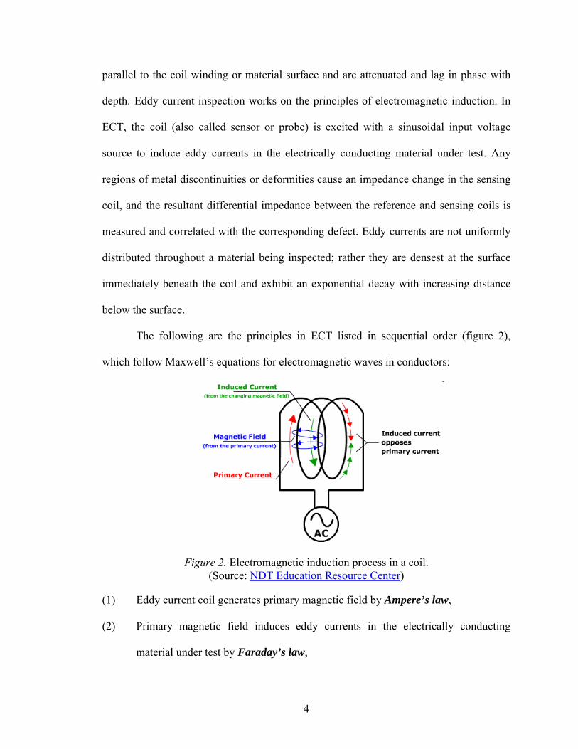
The following are the principles in ECT listed in sequential order (figure 2),
which follow Maxwell’s equations for electromagnetic waves in conductors:
Figure 2. Electromagnetic induction process in a coil. (Source: NDT Education Resource Center)
(1) Eddy current coil generates primary magnetic field by Ampere’s law,
(2) Primary magnetic field induces eddy currents in the electrically conducting
material under test by Faraday’s law,
4
(3) Eddy currents generate secondary magnetic field opposing the primary magnetic
field by Lenz’s law,
(4) Results in a coil impedance change, and
(5) Impedance change is measured, analyzed and correlated with metal proximity and
thickness.
The peak-to-peak amplitude and phase of the eddy current signal provides
information about the defect severity or proximity and defect location or depth
(thickness) respectively. Defects perpendicular to eddy current flow cause maximum coil
impedance change categorized by large signal amplitude and high sensitivity compared to
defects parallel to eddy current flow that results in minimal change in coil impedance
categorized by a small response and low sensitivity.
1.2 Operating Variables
The following operating variables play an important role in eddy current
inspection:
(1) Coil Impedance )LjX( RZ += – It depends on the AC resistance ( )R of the
copper wire and the inductive reactance ( )LX . Phase is given by: RXTan L=φ .
The instantaneous voltage across the inductor due to a change in impedance is:
( ) ( )dt
tdiLtv Δ= . The impedance change is the difference in impedance
measurement with the coil placed over the metal and the coil over free space (air)
i.e., airLL . For a input sinusoidal AC drive through the inductor,
ft
L −=Δ
(I P( )ti )π2sin= , the resultant output voltage is, ( ) ( )ftILftv P ππ 22 Δ cos= .
Therefore the phase of the current lags that of the voltage by 90°.
5
(2) Electrical Conductivity ( )σ – The measurement is based on International
Annealed Copper Standard (IACS). In this system, the conductivity of annealed,
unalloyed copper is arbitrarily rated at 100%, and the conductivities of other
metals and alloys are expressed as percentages of this standard.
(3) Magnetic Permeability ( )μ – It is defined as the ratio of magnetic field strength
( )B and the amount of magnetic flux ( )H within the material, which is a nearly a
constant for small changes in field strength. Magnetic permeability strongly
influences the eddy-current response. The relative permeability, rμ is the ratio of
the permeability ⎟⎠⎞
⎜⎝⎛ ×=, μ −
mH6 of a specific
material to the permeability of free space
umFor 102566650.1minAlu
⎟⎠⎞
⎜⎝⎛ ×= −
27
0 104ANπμ , and is equal to
unity for non-magnetic metals. For Aluminum rμ is 1.000022.
(4) Electromagnetic Coupling – The coupling of magnetic field to the material
surface is important in eddy current testing. This coupling depends on the type of
probes used, which may be surface or encircling probes.
(5) “Lift-off” Factor – Relates to surface probes, and is defined as the distance
between the probe coil and the material under test, which translates to a change in
coil impedance. Uniform and small lift-off is preferred to achieve better
sensitivity to defect detection.
(6) Edge Effect – The distortion of eddy currents due to the inspection coil
approaching the end or edge of a part being inspected. It is difficult to eliminate
6
edge effects due to practical constraints on coil sizes, as they are application
dependent. Scanning in a line parallel to the edge can minimize edge effects.
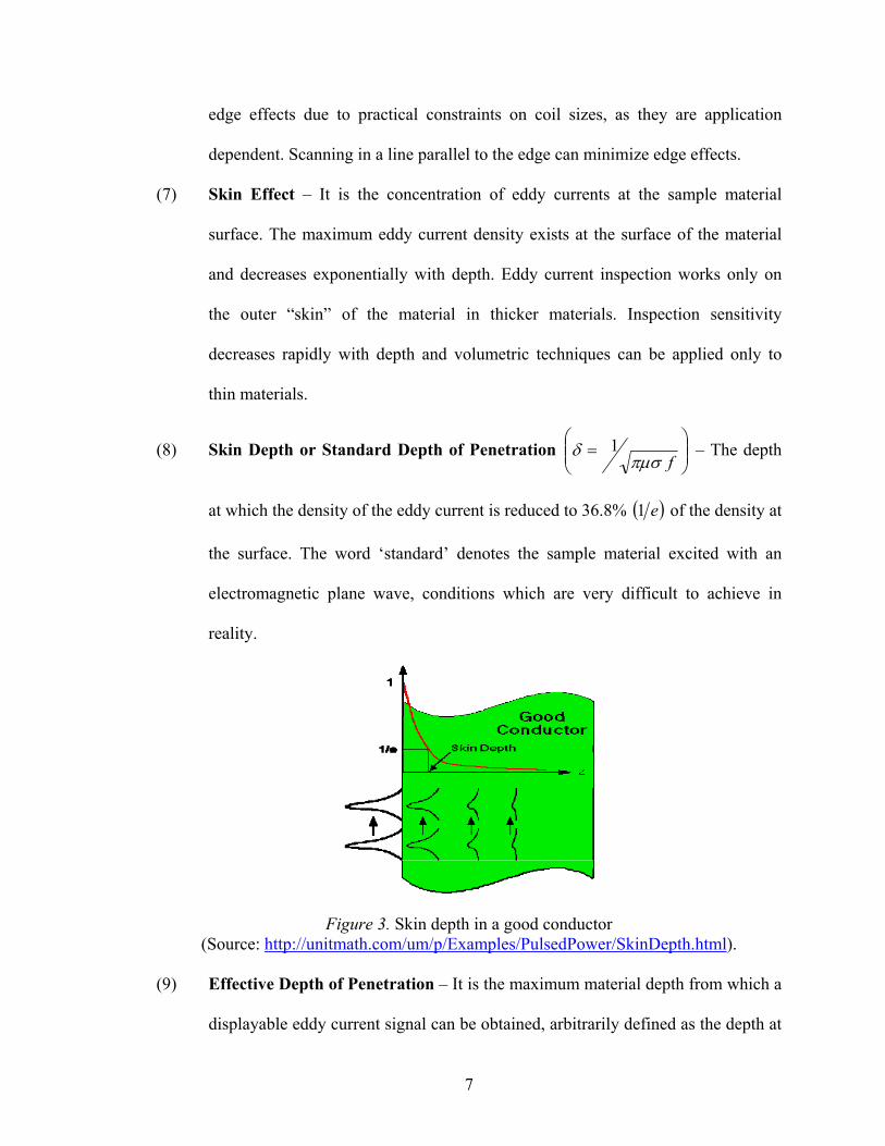
(7) Skin Effect – It is the concentration of eddy currents at the sample material
surface. The maximum eddy current density exists at the surface of the material
and decreases exponentially with depth. Eddy current inspection works only on
the outer “skin” of the material in thicker materials. Inspection sensitivity
decreases rapidly with depth and volumetric techniques can be applied only to
thin materials.
(8) Skin Depth or Standard Depth of Penetration ⎟⎟⎠
⎞⎜⎜⎝
⎛=
fπμσδ 1 – The depth
at which the density of the eddy current is reduced to 36.8% ( )e1 of the density at
the surface. The word ‘standard’ denotes the sample material excited with an
electromagnetic plane wave, conditions which are very difficult to achieve in
reality.
Figure 3. Skin depth in a good conductor (Source: http://unitmath.com/um/p/Examples/PulsedPower/SkinDepth.html).
(9) Effective Depth of Penetration – It is the maximum material depth from which a
displayable eddy current signal can be obtained, arbitrarily defined as the depth at
7
which eddy current density has decreased to 5% of the surface eddy current
density.
(10) Inspection Frequency ( )f – Typically depends on the metal being inspected and
can range from 60 Hz to 6 MHz or more. Non-magnetic metals are inspected at a
few KHz and lower frequencies are used for magnetic metals due to their low
penetration depth with higher frequencies used only to inspect surface conditions.
Factors influencing inspection frequency are material thickness, depth of
penetration, degree of sensitivity or resolution and purpose of inspection. Often a
compromise has to be achieved between these various factors for a given
application.
(11) Inspection Coils – Coils come in a variety of shapes and sizes that are normally
specific to an application. Coil shapes are mainly dependent on external or
internal inspection desired and sizes are dependent on the degree of sensitivity
desired. A more in-depth discussion on coil design and characterization is
presented in Chapter 3 - Coil Design and Characterization.
1.3 Principles of Operation
Eddy current inspection in this project is achieved by using an in-house designed
automated data acquisition system providing the following functionality:
(1) The inspection coil is excited with a range of frequencies at each lift-off distance
using a multi-frequency technique.
(2) The output signal of the inspection coil is modulated by the metal sample being
inspected.
(3) Inspection coil output signal is processed prior to amplification.
8
(4) Amplification of the inspection coil signals using a pre-amplifier.
(5) The amplified signals are digitized using a PCI digitizer followed by amplitude
and phase analysis of signals by a computer using an in-house developed data
acquisition application written in National Instruments LabVIEW 8.0.
(6) The output signals are displayed, measured and the corresponding data recorded
simultaneously into ‘Text’ files.
(7) The raw data is processed using an in-house developed 32-bit Windows dynamic
link library (DLL) software application written in Microsoft® Visual Basic 6.0.
(8) The processed data is used in 2D graphical analysis using Microsoft® Excel.
(9) Handling of the metal sample being inspected and support of inspection coil
assembly.
1.4 Previous Eddy Current NDT Research Work
According to Dodd and Deeds [15], eddy-current coil problems fall in the
intermediate frequency region. They proposed a closed-form theoretical solution of an
air-cored coil above a metallic plate using the vector potential as opposed to electric and
magnetic fields. The differential equations for the vector potential are derived from
Maxwell’s equations, assuming cylindrical symmetry. The derived result for inductance
is [16]:
( ) ( ) ( ) ( )∫∞
=Δ0
6
2
ααφαααω dAPKL
where
( ) ( )( ) ( )( )( )( ) ( )( ) c
c
ee
1
1
21111
21111
α
α
αααααααααααααααα
αφ−++−−−−+−−+
=
9
02
1 ωσμαα j+=
( ) ( )2212
21
20
rrllN
K−−
=πμ
( ) ( )∫=2
1
1
r
r
dxxJPα
α
αα
( ) ( )221 ll eeA ααα −− −=
where α is an integration variable, ω is the angular frequency of the excitation signal, μ
and σ are the permeability and conductivity of the metal sample, N is the number of turns
in the coil, r1 and r2 are inner and outer radii of the coil, l1 and l2 are the heights of the
bottom and top of the coil, c is the metal sample thickness, μ0 is the permeability of free
space, and J1(x) is a first-order Bessel function of the first kind. Dodd and Deeds have
shown that theoretical and experimental values of impedance are in agreement at higher
frequencies as measurements at lower frequencies are difficult to make with poor
accuracy.
Yin et al. [16, 17] have employed the technique of using phase signature for
thickness detection of non-magnetic metal plates, and shown that phase is independent of
lift-off if the pole distance (distance between the excitation and pickup coils) is much
larger than the radius of the coils. Their research uses two eddy-current sensors (dual
probes) with a single sided measurement. The phase technique is in contrast to using the
magnitude of the eddy-current signal which generally decreases with increasing lift-off.
Placko et al. [18] have shown a technique for simultaneous distance and thickness
measurements of zinc-aluminum coating on a steel substrate using an eddy-current sensor
with a ‘H’ shaped ferromagnetic core. For distance measurements, they consider a
10
11
metallic body placed near the sensor which modifies the path of the magnetic field and
changes the reluctance independent of the physical properties of the metal, apart from
introducing eddy current losses. The reluctance and eddy current losses are measured
separately, from the current in the coil, using a synchronous detection with quadrature or
in-phase reference signal with respect to the driving voltage. For non-contact thickness
measurements, the two quadrature and in-phase components are coupled to the distance
of the plate, and to the thickness of the coating.
Wincheski et al. [19] in an effort to enhance the effectiveness of material
thickness measurements developed a flux focusing eddy current probe at NASA Langley
Research Center. The flux focusing eddy current probe uses a ferromagnetic material
between the drive and pickup coils in order to focus the magnetic flux of the probe.
Output voltage dependency as a function of material thickness is used for thickness
estimation of conducting materials from a single sided measurement.
1.5 Thesis Layout
This thesis is structured with a theoretical explanation followed by experimental
design. Chapter 2 provides the mathematical background, and chapters 3, 4, 5 explain the
coil design and characterization, experimental setup and design, and results respectively.
Finally, chapter 6 provides a conclusion, summarizes the results of this research study
and proposes ideas for future work.
Chapter 2
Mathematical Background
In this chapter, the behavior of electromagnetic waves in conductors is discussed
along with the mathematical equations for the physical E and B fields starting from
Maxwell’s equations for a linear, homogeneous medium. An important property called
skin depth that results out of wave attenuation in conductors is also discussed. The
mathematical background presented in this chapter is primarily adopted from
“Introduction to Electrodynamics” (3rd Edition) by David J. Griffiths [4].
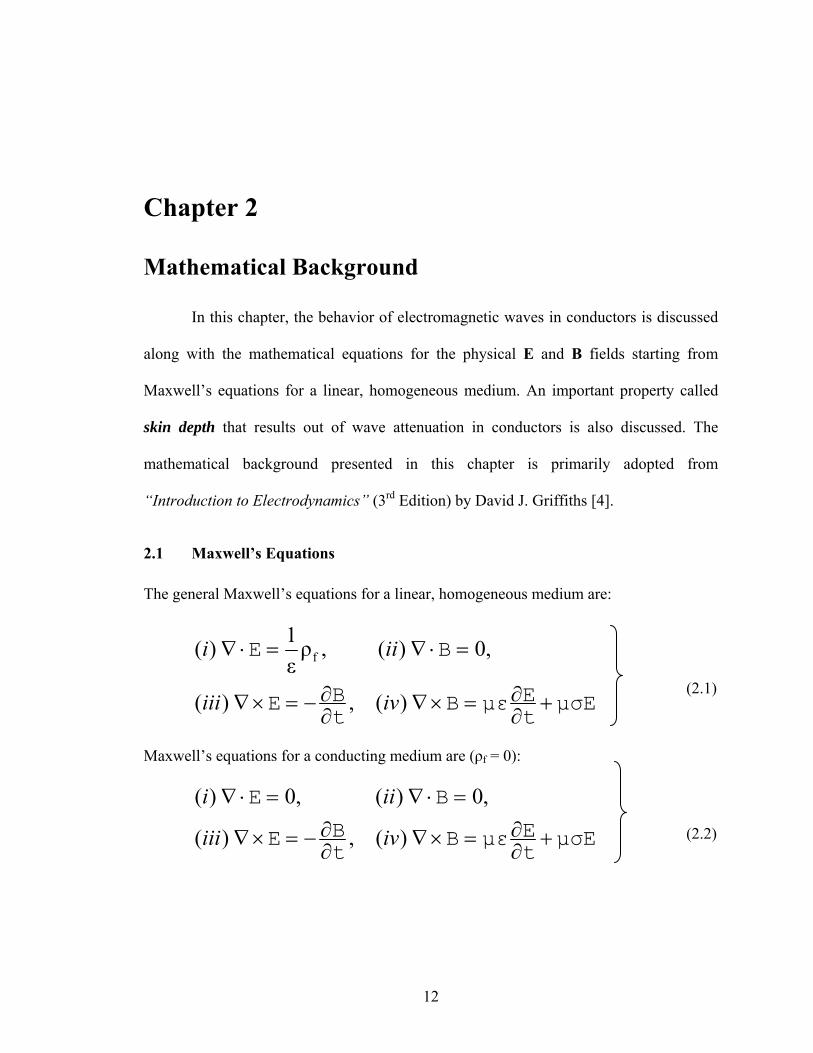
2.1 Maxwell’s Equations The general Maxwell’s equations for a linear, homogeneous medium are:
μσE
tEμεB
tBE
BE
+∂∂=×∇
∂∂−=×∇
=⋅∇=⋅∇
)(,)(
,0)(,ρε1)( f
iviii
iii
(2.1)
Maxwell’s equations for a conducting medium are (ρf = 0):
μσEtEμεB
tBE
BE
+∂∂=×∇
∂∂−=×∇
=⋅∇=⋅∇
)(,)(
,0)(,0)(
iviii
iii (2.2)
12

2.2 Electric and Magnetic Field Waves in Conductors
The second order wave equations for E and B fields are obtained by applying the curl to
Faraday’s and Ampere’s laws in equation (2.2):
tE
tE
zE xxx
∂∂
+∂∂
=∂∂
μσμε 2
2
2
2
, .2
2
2
2
tB
tB
zB yyy
∂
∂+
∂
∂=
∂
∂μσμε
These second order wave equations for E and B fields still have monochromatic plane-
wave solutions of the form,
( ) ( ) ⎟⎟⎠
⎞⎜⎜⎝
⎛⎟⎟⎠
⎞⎜⎜⎝
⎛
==)-~(~,~,
)-~(~,~00
tzkieBtzB
tzkieEtzE
ωω (2.3)
resulting in the modified wave equations:
yy
xx Bi
zB
EizE ~][
~,~][
~2
2
22
2
2
μσωμεωμσωμεω +−=∂
∂+−=
∂∂
with a complex “wave number” k~ :
]2[2~ μσωμεω ik +−= (2.4) or ,~ κikk +=
where,
k~ - complex wave number;
k - phase constant (radians per unit length); and
κ - attenuation constant (nepers per unit length).
Relative values of conduction current density ( )EJ σ= , and displacement current
density ⎟⎠⎞
⎜⎝⎛
∂∂
=∂∂
tE
tD ε determine whether a given material acts like a good conductor or a
good dielectric (Source: Third-year Electromagnetism by Robert D. Watson, School of
Mathematics and Physics, University of Tasmania).
13
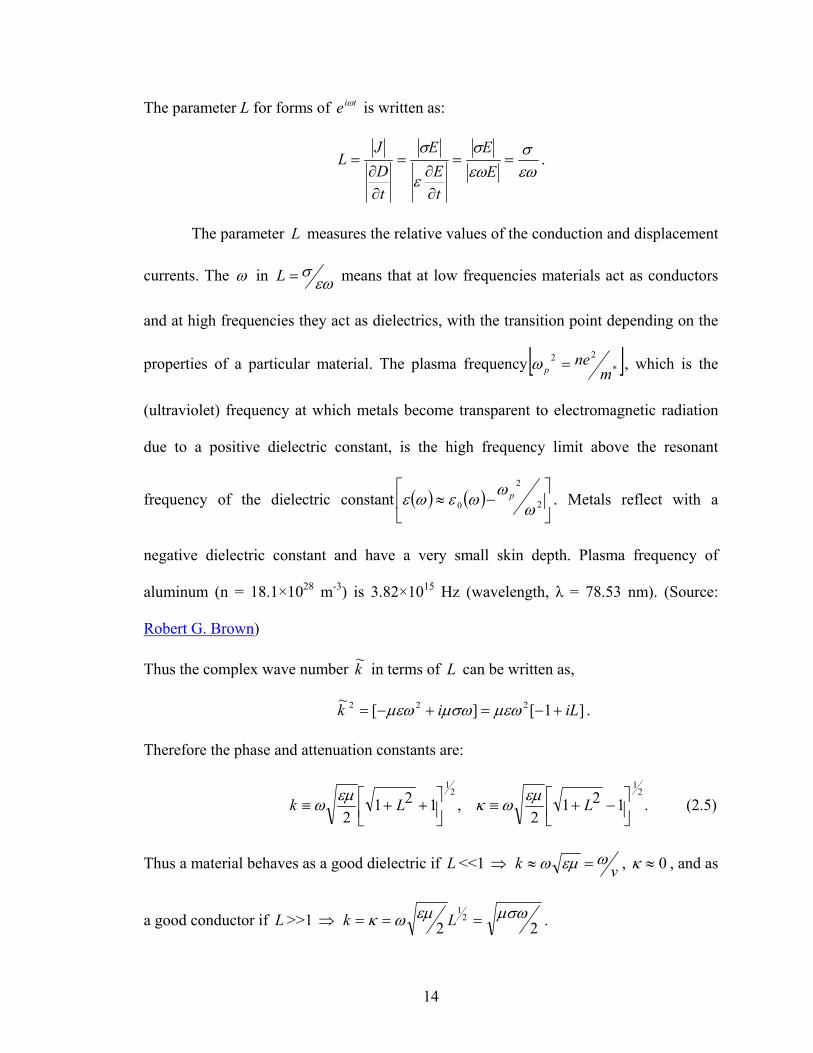
The parameter L for forms of is written as: tie ω
εωσ
εωσ
ε
σ==
∂∂
=
∂∂
=E
E
tE
E
tDJ
L .
The parameter measures the relative values of the conduction and displacement
currents. The
L
ω in εωσ=L means that at low frequencies materials act as conductors
and at high frequencies they act as dielectrics, with the transition point depending on the
properties of a particular material. The plasma frequency [ ]*22
mne
p =ω , which is the
(ultraviolet) frequency at which metals become transparent to electromagnetic radiation
due to a positive dielectric constant, is the high frequency limit above the resonant
frequency of the dielectric constant ( ) ( ) ⎥⎦
⎤⎢⎣
⎡−≈ 2
2
0 ωωωεωε p . Metals reflect with a
negative dielectric constant and have a very small skin depth. Plasma frequency of
aluminum (n = 18.1×1028 m-3) is 3.82×10¹⁵ Hz (wavelength, λ = 78.53 nm). (Source:
Robert G. Brown)
Thus the complex wave number k~ in terms of can be written as, L
]1[][~ 222 iLik +−=+−= μεωμσωμεω . Therefore the phase and attenuation constants are:
.1212
,1212
21
21
⎥⎦⎤
⎢⎣⎡ −+≡⎥⎦
⎤⎢⎣⎡ ++≡ LLk εμωκεμω (2.5)
Thus a material behaves as a good dielectric if <<1 ⇒ L vk ωεμω =≈ , 0≈κ , and as
a good conductor if >>1 ⇒ L 22 μσωεμωκ === 2
1Lk .
14
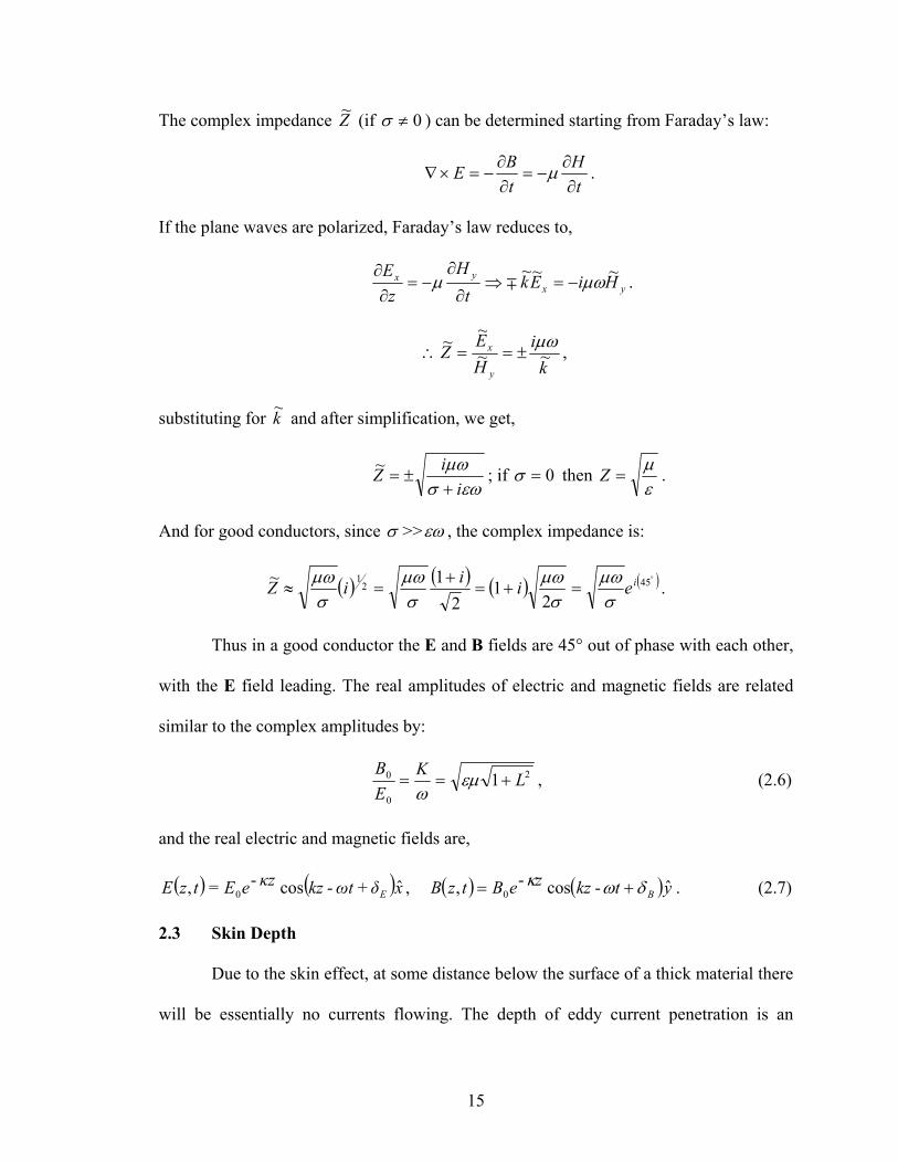
The complex impedance Z~ (if 0≠σ ) can be determined starting from Faraday’s law:
tH
tBE
∂∂
−=∂∂
−=×∇ μ .
If the plane waves are polarized, Faraday’s law reduces to,
yxyx HiEk
tH
zE ~~~ μωμ −=⇒
∂
∂−=
∂∂ ∓ .
ki
HE
Zy
x ~~~
~ μω±==∴ ,
substituting for k~ and after simplification, we get,
εωσμω
iiZ+
±=~ ; if 0=σ then εμ
=Z .
And for good conductors, since σ >>εω , the complex impedance is:
( ) ( ) ( ) ( )°=+=+
=≈ 4521
21
21~ ieiiiZ
σμω
σμω
σμω
σμω .
Thus in a good conductor the E and B fields are 45° out of phase with each other,
with the E field leading. The real amplitudes of electric and magnetic fields are related
similar to the complex amplitudes by:
2
0
0 1 LKEB
+== εμω
, (2.6)
and the real electric and magnetic fields are,
( ) ( )xδtωkzzκeEtzE E ˆ+-cos-=, 0 , ( ) ( )ytkzzeBtzB B ˆ-cos-, 0 δωκ += . (2.7)
2.3 Skin Depth
Due to the skin effect, at some distance below the surface of a thick material there
will be essentially no currents flowing. The depth of eddy current penetration is an
15
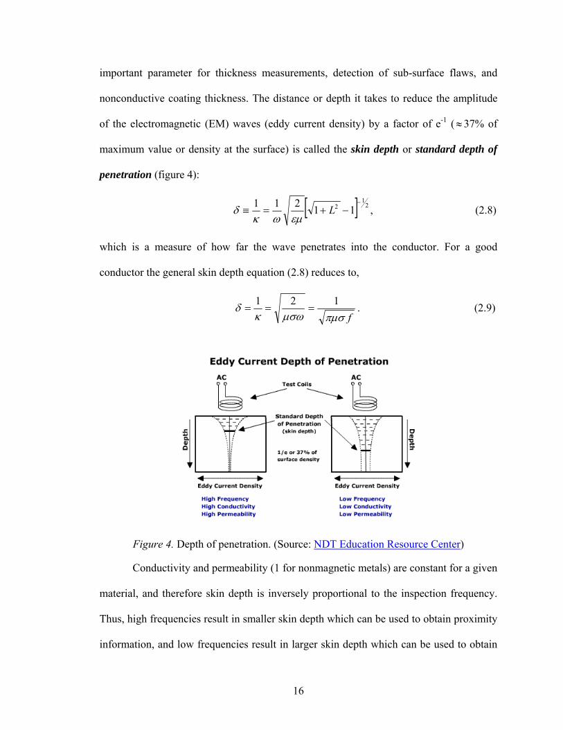
important parameter for thickness measurements, detection of sub-surface flaws, and
nonconductive coating thickness. The distance or depth it takes to reduce the amplitude
of the electromagnetic (EM) waves (eddy current density) by a factor of e-1 (≈37% of
maximum value or density at the surface) is called the skin depth or standard depth of
penetration (figure 4):
[ ] 21
2 11211 −−+=≡ L
εμωκδ , (2.8)
which is a measure of how far the wave penetrates into the conductor. For a good
conductor the general skin depth equation (2.8) reduces to,
fπμσμσωκδ 121
=== . (2.9)
Figure 4. Depth of penetration. (Source: NDT Education Resource Center)
Conductivity and permeability (1 for nonmagnetic metals) are constant for a given
material, and therefore skin depth is inversely proportional to the inspection frequency.
Thus, high frequencies result in smaller skin depth which can be used to obtain proximity
information, and low frequencies result in larger skin depth which can be used to obtain
16
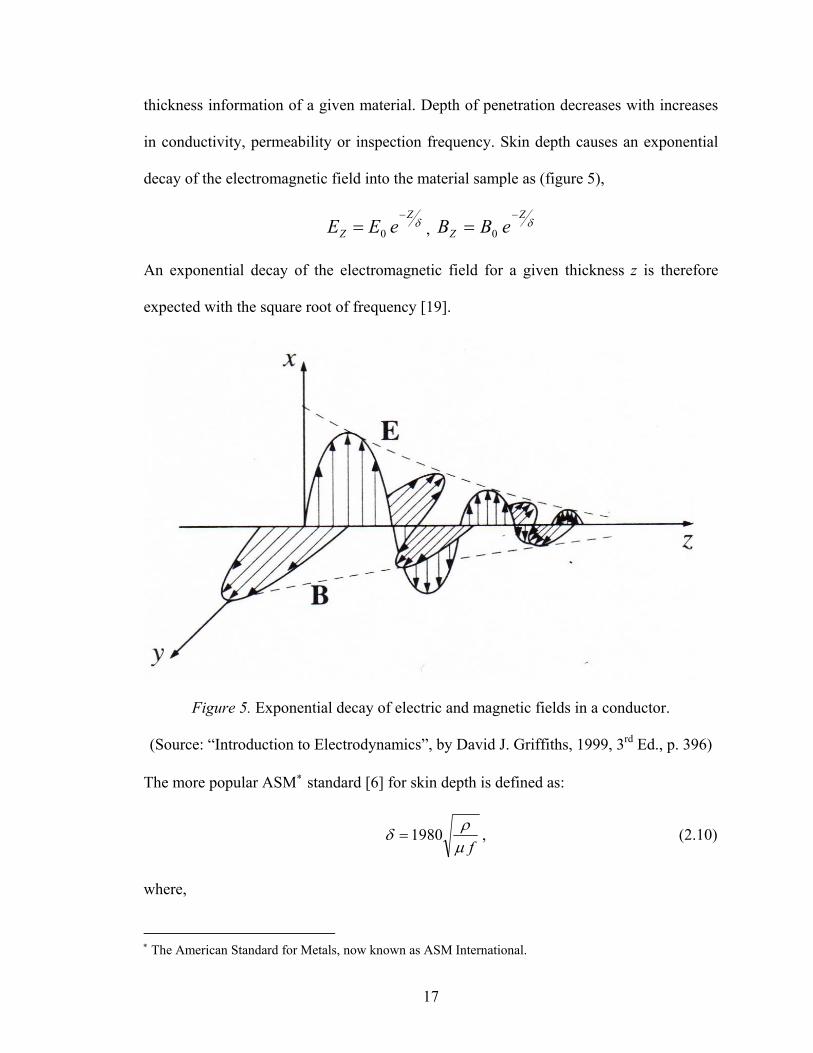
thickness information of a given material. Depth of penetration decreases with increases
in conductivity, permeability or inspection frequency. Skin depth causes an exponential
decay of the electromagnetic field into the material sample as (figure 5),
δZ
Z eEE−
= 0 , δZ
Z eBB−
= 0
An exponential decay of the electromagnetic field for a given thickness z is therefore
expected with the square root of frequency [19].
Figure 5. Exponential decay of electric and magnetic fields in a conductor.
(Source: “Introduction to Electrodynamics”, by David J. Griffiths, 1999, 3rd Ed., p. 396)
The more popular ASM∗ standard [6] for skin depth is defined as:
fμρδ 1980= , (2.10)
where,
∗ The American Standard for Metals, now known as ASM International.
17
δ - standard depth of penetration (inches);
ρ - material resistivity (ohm-centimeters);
μ - material magnetic permeability (1 for nonmagnetic materials); and
f - inspection frequency (hertz).
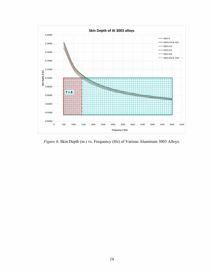
Figure 6 shows a plot of skin depth (in.) versus frequency (Hz) for various types
of Al 3003 alloys. The plot was generated using equation (2.10). As can be seen, skin
depth decreases exponentially with increase in inspection frequency. Appendix A
provides a detailed explanation of the different types of Al 3003 alloys. The shaded box
in figure 6 shows the working range for inspection frequency (500 Hz – 6 KHz) and
metal thickness (0.016” – 0.100”) used in this project. The red patterned box indicates the
potential range of frequencies that can be utilized for thickness (single/double) estimation
as long as thickness is less than skin depth at a specific frequency.
18
19
Skin Depth of Al 3003 alloys
0.00000
0.02000
0.04000
0.06000
0.08000
0.10000
0.12000
0.14000
0.16000
0.18000
0.20000
0 500 1000 1500 2000 2500 3000 3500 4000 4500 5000 5500 6000 6500
Frequency, F (Hz)
Skin Dep
th, δ
(in)
3003‐O
3003‐H14 & ‐H12
3003‐H12
3003‐H14
3003‐H18
3003‐H24 & ‐H28
T < δ
Figure 6. Skin Depth (in.) vs. Frequency (Hz) of Various Aluminum 3003 Alloys.
Chapter 3
Coil Design and Characterization
The essential part of any eddy current inspection system is the inspection coil or
probe, as it is the probe that dictates the probability of detection and the reliability of
characterization. Eddy current probes come in a variety of shapes, cross-sections, sizes
and configurations, giving the user flexibility in custom designing a probe for a specific
application or inspection. Apart from the component geometry of the eddy current probe,
factors such as impedance matching, magnetic field focusing and environmental
conditions play a crucial role in its design and development. For precise detection of
flaws in the metal under test, it is important for the eddy current flow to be as nearly
perpendicular to the flaw as possible. On the other hand, if the eddy current flow is
parallel to the flaw, there will be little or no response from the inspection coil as the
currents are hardly distorted. In this chapter, a discussion on eddy current sensor
components and coil characterization is presented.
3.1 Eddy Current Sensor Components
The eddy current sensor has the following components: physical coil (reference
and sensing) specifications, mode of operation, core type, coil configuration, shielding
and loading. For a given application, choosing the right coil design is the most important
task in any eddy current probe design process. With the target application in this project
being the measurement of proximity and thickness of metal sheets, a single probe dual
20
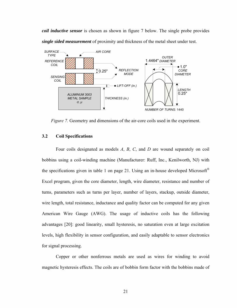
coil inductive sensor is chosen as shown in figure 7 below. The single probe provides
single sided measurement of proximity and thickness of the metal sheet under test.
REFLECTION MODE
ALUMINUM 3003 METAL SAMPLE
σ, μ
REFERENCE COIL
SENSING COIL
THICKNESS (in.)
LIFT-OFF (in.)
0.25"
AIR CORESURFACE TYPE
1.0"1.4464"
0.25"LENGTH
CORE DIAMETER
OUTER DIAMETER
NUMBER OF TURNS: 1440
Figure 7. Geometry and dimensions of the air-core coils used in the experiment.
3.2 Coil Specifications
Four coils designated as models A, B, C, and D are wound separately on coil
bobbins using a coil-winding machine (Manufacturer: Ruff, Inc., Kenilworth, NJ) with
the specifications given in table 1 on page 21. Using an in-house developed Microsoft®
Excel program, given the core diameter, length, wire diameter, resistance and number of
turns, parameters such as turns per layer, number of layers, stackup, outside diameter,
wire length, total resistance, inductance and quality factor can be computed for any given
American Wire Gauge (AWG). The usage of inductive coils has the following
advantages [20]: good linearity, small hysteresis, no saturation even at large excitation
levels, high flexibility in sensor configuration, and easily adaptable to sensor electronics
for signal processing.
Copper or other nonferrous metals are used as wires for winding to avoid
magnetic hysteresis effects. The coils are of bobbin form factor with the bobbins made of
21
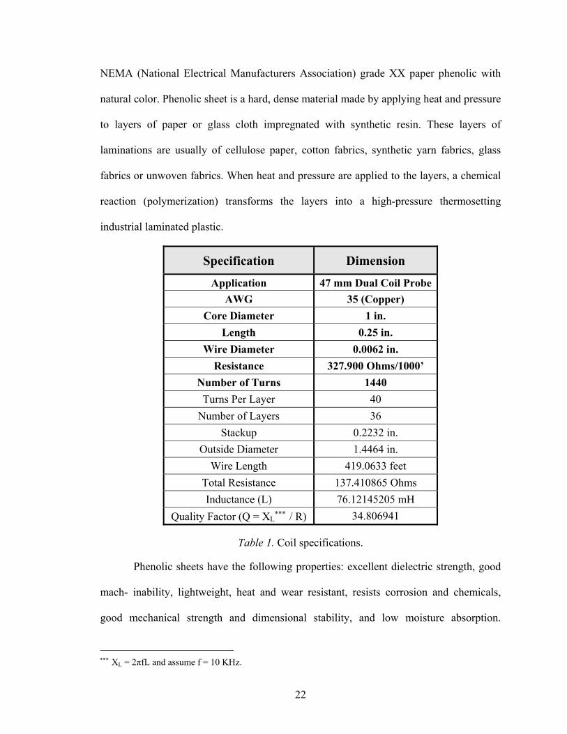
NEMA (National Electrical Manufacturers Association) grade XX paper phenolic with
natural color. Phenolic sheet is a hard, dense material made by applying heat and pressure
to layers of paper or glass cloth impregnated with synthetic resin. These layers of
laminations are usually of cellulose paper, cotton fabrics, synthetic yarn fabrics, glass
fabrics or unwoven fabrics. When heat and pressure are applied to the layers, a chemical
reaction (polymerization) transforms the layers into a high-pressure thermosetting
industrial laminated plastic.
Specification Dimension
Application 47 mm Dual Coil Probe AWG 35 (Copper)
Core Diameter 1 in. Length 0.25 in.
Wire Diameter 0.0062 in. Resistance 327.900 Ohms/1000’
Number of Turns 1440 Turns Per Layer 40
Number of Layers 36 Stackup 0.2232 in.
Outside Diameter 1.4464 in. Wire Length 419.0633 feet
Total Resistance 137.410865 Ohms Inductance (L) 76.12145205 mH
Quality Factor (Q = XL∗∗∗ / R) 34.806941
Table 1. Coil specifications.
Phenolic sheets have the following properties: excellent dielectric strength, good
mach- inability, lightweight, heat and wear resistant, resists corrosion and chemicals,
good mechanical strength and dimensional stability, and low moisture absorption.
∗∗∗ XL = 2πfL and assume f = 10 KHz.
22
Phenolic sheets find applications in terminal boards, switches, gears, bearings, wear
strips, gaskets, washers, transformers, machining components, industrial laminates, coil
bobbins, etc., to name a few.
3.3 Mode of Operation
The two coils of the eddy current test probe are set up in reflection mode (Source:
NDT Education Resource Center) i.e., the coil closest to the metal sheet is called the
sensing coil and coil farthest from the metal sheet is called the reference coil. Reflection
mode probes have a higher gain compared to their differential counterpart when tuned to
a specific frequency and are less sensitive to drift problems. They also have a wider
frequency range of operation, as the probes do not need to balance the driver and pickup
coils, with resolution compromised at certain frequencies being the only drawback.
Reflection probes are almost invariably difficult to design and manufacture thereby
making them more expensive. Coil windings of the reference and sensing coils are in
opposition as in differential mode. The spacing between the two coils is set to 0.25” and
this minimum spacing is chosen such that the reference coil is not significantly
influenced by the presence of metal at the face of the probe. On the other hand, the
maximum spacing is only limited by the desire to keep the probe a reasonable size.
3.4 Core Type
The core of the coils is essentially air-core, also called as formers. Core can also
be a solid material of hard magnetic or soft magnetic or nonmagnetic type. Both the hard
and soft versions of the magnetic material increase the coil inductance whereas the
nonmagnetic materials decrease the coil inductance. The hard magnetic materials retain
their magnetism after the magnetizing source has been removed effectively turning into
23
permanent magnets, but the soft magnetic materials lose their magnetism in the absence
of the magnetizing source. Sensitivity of eddy current testing also depends on the type of
core used in a coil and can swing either up or down depending on magnetic or
nonmagnetic respectively.
It is important to maintain the current in the coil as low as possible. As current
increases, the inductance increases as the coil expands due to a rise in temperature.
Additionally, effects of magnetic hysteresis come into play when magnetic cores are
used. Examples of ferrous cores are iron-powder, ferrite, laminated and tuning cores,
slugs and toroids where in the core of a coil is adjustable. Similarly cores of nonferrous
metals can include brass, copper and silver.
3.5 Coil Configuration
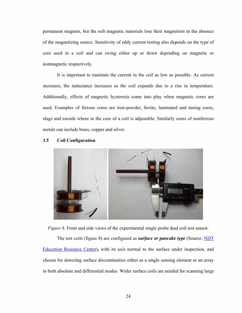
Figure 8. Front and side views of the experimental single probe dual coil test sensor.
The test coils (figure 8) are configured as surface or pancake type (Source: NDT
Education Resource Center), with its axis normal to the surface under inspection, and
chosen for detecting surface discontinuities either as a single sensing element or an array
in both absolute and differential modes. Wider surface coils are needed for scanning large
24
areas for surface defects and for greater depth of penetration. However, as coil diameter
increases, sensitivity decreases.
3.6 Probe Shielding and Loading
Shielding an eddy current probe from electromagnetic interference (EMI) is one
of the most difficult of challenges that an engineer encounters during the design phase
(Source: NDT Education Resource Center). Shielding is a technique used to minimize the
interaction of the external forces such as noise and other spurious signals, which are some
of the many sources of EMI, from the magnetic field of the eddy current probe within its
immediate surroundings. Shielding is also employed to reduce edge effect problems and
the effects of magnetic fasteners in the test region. Shielding and loading act together to
limit the spread and focus the magnetic field to a narrow area on the test material.
Eddy current probes are manufactured in both shielded and un-shielded versions
with shielded versions available in a variety of housings made of magnetic and non-
magnetic metals and plastic. Both the necessity and type of shielding are dependent on
the end application of the eddy current probe. Area of the flaw to be detected, sensitivity
and resolution are some of the main criteria that need to be considered in deciding the
necessity and appropriate type of shielding. Probes loaded with ferrite cores tend to be
more sensitive and less prone to lift-off and wobble effects compared to its air core
counterpart as ferrite cores focus the magnetic field to the center of the probe due to the
magnetic flux generated by the coil traveling through the ferrite core rather than air as in
air core coils.
25
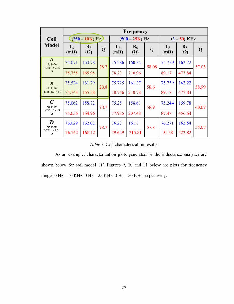
3.7 Coil Characterization
Once the design is chosen, the next step is to match and characterize the coil
impedance, which is the critical step for coil-based inductor designs. The four coil
models A, B, C, and D are characterized in free air using a QuadTech 1910 Inductance
Analyzer to verify linearity of operation over multiple frequency ranges. Table 2 on page
26 lists the characterization results for the inductance coil models ‘A’, ‘B’, ‘C’ and ‘D’.
The table specifies the number of turns (N), direct current resistance (DCR), secondary
inductance (LS), secondary (effective AC) resistance (RS), and the quality factor (Q).
Each coil is connected to the Inductance Analyzer, scanned through each frequency range
and LS, RS, Q are measured using an in- house developed Microsoft® Visual Basic GUI.
LS and RS are measured at the lower and upper bound of a given frequency range, while
Q is measured at the upper bound of the frequency range.
Coil impedances are matched for a given frequency range and if necessary,
number of turns of a coil is reduced in small whole turns in order to match the impedance
with the other coils. A set of two coils must be matched as close as possible in impedance
by maintaining an almost constant inductance value over a wide frequency range. From
the above table we can clearly observe that coil models ‘A’ and ‘B’ is most closely
matched pair in impedance over all parameters in the 250 Hz to 10 KHz frequency range
among the four coil models. This implies that coil models ‘A’ and ‘B’ are the right choice
for the dual coil probe and have a linear operating region within the above frequency
range. One of the coils (in this case model ‘B’) is used as a reference coil and the other
coil (model ‘A’) is used as a sensing coil to measure a change in impedance.
26
Coil Model
Frequency (250 – 10K) Hz (500 – 25K) Hz (3 – 50) KHz
LS (mH)
RS (Ω) Q LS
(mH) RS (Ω) Q LS
(mH) RS (Ω) Q
A N: 1450
DCR: 159.95 Ω
75.071 160.7828.7
75.286 160.34 58.08
75.759 162.2257.03
75.755 165.98 78.23 210.96 89.17 477.84
B N: 1450
DCR: 160.4 Ω
75.524 161.7928.8
75.725 161.37 58.6
75.759 162.2258.99
75.748 165.38 78.746 210.78 89.17 477.84
C N: 1450
DCR: 158.23 Ω
75.062 158.7228.7
75.25 158.61 58.9
75.244 159.7860.07
75.636 164.96 77.985 207.48 87.47 456.64
D N: 1550
DCR: 161.31 Ω
76.029 162.0228.7
76.23 161.7 57.8
76.271 162.5455.07
76.762 168.12 79.629 215.81 91.58 522.82
Table 2. Coil characterization results.
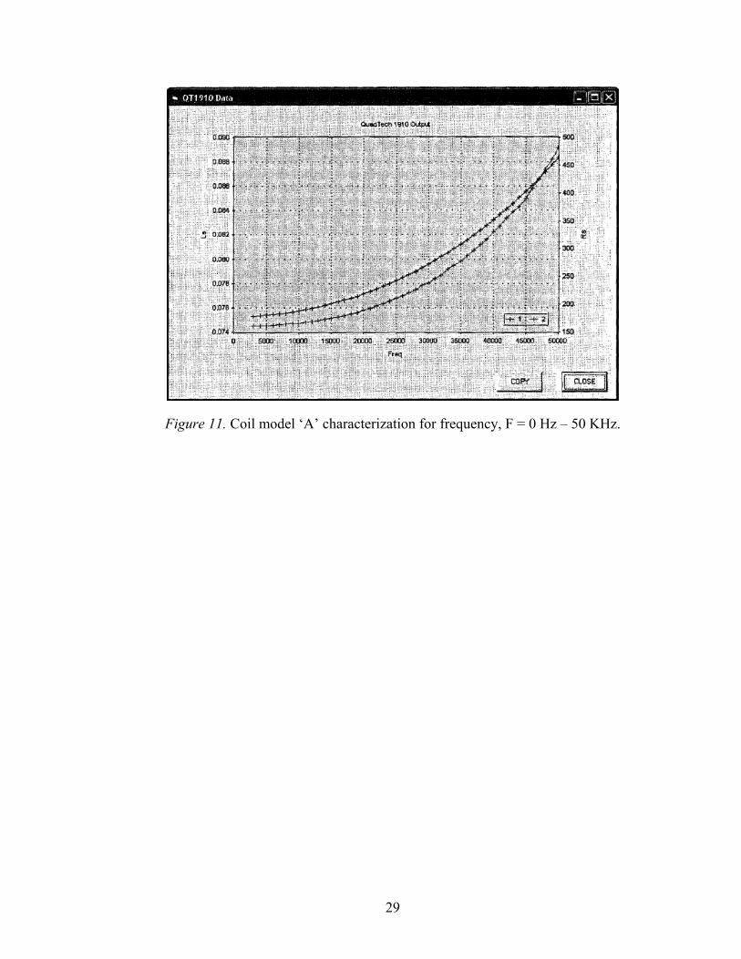
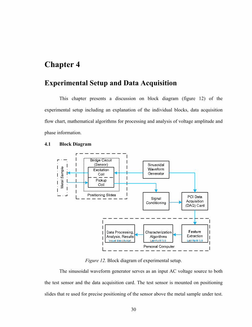
As an example, characterization plots generated by the inductance analyzer are
shown below for coil model ‘A’. Figures 9, 10 and 11 below are plots for frequency
ranges 0 Hz – 10 KHz, 0 Hz – 25 KHz, 0 Hz – 50 KHz respectively.
27
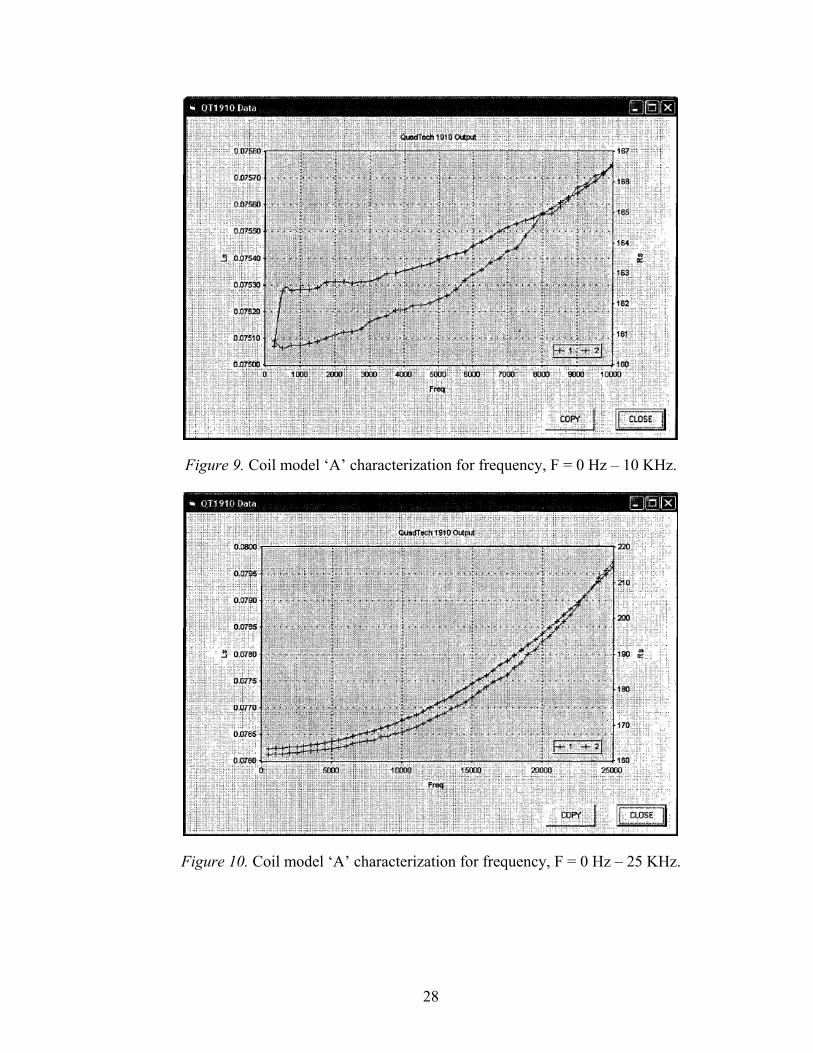
Figure 9. Coil model ‘A’ characterization for frequency, F = 0 Hz – 10 KHz.
Figure 10. Coil model ‘A’ characterization for frequency, F = 0 Hz – 25 KHz.
28
29
Figure 11. Coil model ‘A’ characterization for frequency, F = 0 Hz – 50 KHz.
Chapter 4
Experimental Setup and Data Acquisition
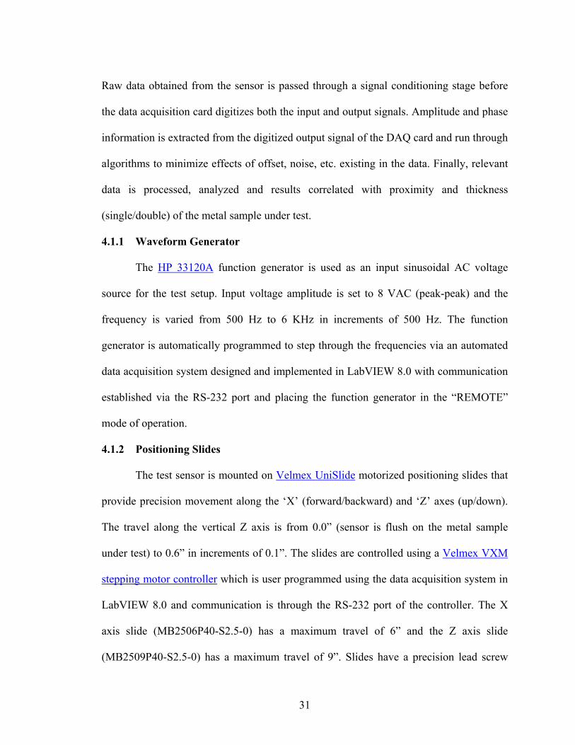
This chapter presents a discussion on block diagram (figure 12) of the
experimental setup including an explanation of the individual blocks, data acquisition
flow chart, mathematical algorithms for processing and analysis of voltage amplitude and
phase information.
4.1 Block Diagram
Figure 12. Block diagram of experimental setup.
The sinusoidal waveform generator serves as an input AC voltage source to both
the test sensor and the data acquisition card. The test sensor is mounted on positioning
slides that re used for precise positioning of the sensor above the metal sample under test.
30
Raw data obtained from the sensor is passed through a signal conditioning stage before
the data acquisition card digitizes both the input and output signals. Amplitude and phase
information is extracted from the digitized output signal of the DAQ card and run through
algorithms to minimize effects of offset, noise, etc. existing in the data. Finally, relevant
data is processed, analyzed and results correlated with proximity and thickness
(single/double) of the metal sample under test.
4.1.1 Waveform Generator
The HP 33120A function generator is used as an input sinusoidal AC voltage
source for the test setup. Input voltage amplitude is set to 8 VAC (peak-peak) and the
frequency is varied from 500 Hz to 6 KHz in increments of 500 Hz. The function
generator is automatically programmed to step through the frequencies via an automated
data acquisition system designed and implemented in LabVIEW 8.0 with communication
established via the RS-232 port and placing the function generator in the “REMOTE”
mode of operation.
4.1.2 Positioning Slides
The test sensor is mounted on Velmex UniSlide motorized positioning slides that
provide precision movement along the ‘X’ (forward/backward) and ‘Z’ axes (up/down).
The travel along the vertical Z axis is from 0.0” (sensor is flush on the metal sample
under test) to 0.6” in increments of 0.1”. The slides are controlled using a Velmex VXM
stepping motor controller which is user programmed using the data acquisition system in
LabVIEW 8.0 and communication is through the RS-232 port of the controller. The X
axis slide (MB2506P40-S2.5-0) has a maximum travel of 6” and the Z axis slide
(MB2509P40-S2.5-0) has a maximum travel of 9”. Slides have a precision lead screw
31
with an advance per turn of 0.025”, advance per step of 0.0000625”, lead screw error less
than 0.0015”/10” and 1 motor revolution is equivalent to 400 steps. UniSlide come with
standard limit switches that are internal and adjustable to set the travel limits on the lead
screw.
4.1.3 Bridge Circuit
LX LS
RX RS
ZX ZS
RB RA
R
AC
V(t)
-
+
+V
-V
RG = 5.6 kΩ
G = 9.82
-
+
+V
-V
OutputA
B
C
D
Wheatstone Bridge Circuit Preamplifier
REFERENCE COIL
SENSING COIL
Figure 13. Wheatstone bridge circuit and preamplifier.
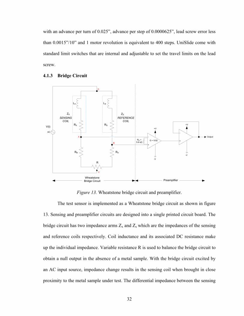
The test sensor is implemented as a Wheatstone bridge circuit as shown in figure
13. Sensing and preamplifier circuits are designed into a single printed circuit board. The
bridge circuit has two impedance arms Zx and Zs which are the impedances of the sensing
and reference coils respectively. Coil inductance and its associated DC resistance make
up the individual impedance. Variable resistance R is used to balance the bridge circuit to
obtain a null output in the absence of a metal sample. With the bridge circuit excited by
an AC input source, impedance change results in the sensing coil when brought in close
proximity to the metal sample under test. The differential impedance between the sensing
32
and reference coils results in an output voltage that serves as an input to the signal
conditioning stage. Equations below show the output voltage of the bridge circuit is a
function of the sensing coil impedance and the input voltage.
( )
( ) ( )tVLjRRR
RRVXXB
BCA ×
++++
=− ω (4.1)
( )( ) ( )tV
LjRRRRRV
SSA
ACB ×
++++
=− ω (4.2)
Equating (4.1) and (4.2),
CBCA VV −− =
( )( )
( )( ) SSA
XXB
A
B
LjRRRLjRRR
RRRR
ωω
++++++
++
= (4.3)
( )( ) ( )tV
LjRRRLjRV
XXB
XXDA ×
++++
=− ωω (4.4)
( )
( ) ( )tVLjRRR
LjRV
SSA
SSDB ×
++++
=− ωω
(4.5)
Equating (4.4) and (4.5),
DBDA VV −− =
( )( )
( )( ) SSA
XXB
SS
XX
LjRRRLjRRR
LjRLjR
ωω
ωω
++++++
=++ (4.6)
quating (4.3) and (4.6), E
( )( )
( )( )RR
RRLjRLjR
A
B
SS
XX
++
=++
ωω
( )( ) S
A
BX Z
RRRR
Z ×++
=
( )tVZV XBA ⋅=−
he component values of the passive devices used in the bridge circuit are given below: T
33
Ω=Ω≅=Ω≅=
≅=
1049916575
RRRRR
mHLL
BA
SX
SX
.1.4 Signal Conditioning
The signal conditioning stage is essentially an op-amp based preamplifier circuit
that has a differential amplifier followed by a voltage follower. Output of the bridge
circuit serves as the input for the differential amplifier that has a closed loop gain of 9.82
set by the gain resistor RG. The voltage follower is used to isolate the high input and low
output impedances and acts as a buffer amplifier to eliminate loading effects. The gain
equation for the differential amplifier is:
4
14.49+
Ω=
GRKG
.1.5 Data Acquisition Card
AlazarTech’s ATS460
4
waveform digitizer for PCI bus is used as a data
acquisition (DAQ) card. This digitizer has two 14 bit resolution analog input channels,
real-time sampling rate of 125 MS/s to 10 KS/s, 8 Million samples of onboard memory,
65 MHz analog input bandwidth, input voltage range of ±20 mV to ±10 V, half length
PCI bus card form factor, analog trigger channel with software-selectable level and slope,
software-selectable AC/DC coupling and 1MΩ/50Ω input impedance, software-selectable
bandwidth limit switch independent for each channel and pre-trigger and post-trigger
capture with multiple record capability. The digitizer is provided with LabVIEW Virtual
Instruments (VIs) that are integrated into the designed data acquisition system.
The DAQ card was setup for data acquisition with the following parameters:
34
Channel A: I/P reference voltage
Channel B: O/P measured voltage
Coupling: AC, 1 MΩ with a -3dB bandwidth of 10 Hz – 65 MHz
Record Length: 2000 points
Number of Records: 1 per channel
Pre-Trigger Depth: 256 points
Clock: Internal, positive edge triggered
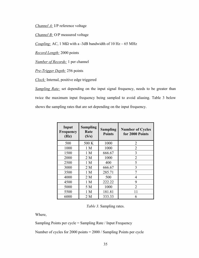
Sampling Rate: set depending on the input signal frequency, needs to be greater than
twice the maximum input frequency being sampled to avoid aliasing. Table 3 below
shows the sampling rates that are set depending on the input frequency.
Input Sampling Sampling Number of Cycles Frequency Rate (Hz) (S/s) Points for 2000 Points
500 500 K 1000 2 1000 1 M 1000 2 1500 1 M 666.67 3 2000 2 M 1000 2 2500 1 M 400 5 3000 2 M 666.67 3 3500 1 M 285.71 7 4000 2 M 500 4 4500 1 M 222.22 9 5000 5 M 1000 2 5500 1 M 181.81 11 6000 2 M 333.33 6
e 3. Sampling rates.
Where,
Points per cycle = Sampling Rate / Input Frequency
cycle
Tabl
Sampling
Number of cycles for 2000 points = 2000 / Sampling Points per
35
The sampling rates satisfy the minimum criteria of greater than two times the
maxim
ition Flow Chart
a flow chart with steps followed in the data
acquisi
um input frequency being sampled, and to minimize the jumps in phase from point
to point, as there will be a trade off with how much phase noise is introduced into the
system by sampling at a higher rate which will distort the phase. Note: The latest version
of ATS460 offered by AlazarTech at the time of this writing has a few more enhanced
features in comparison to the version used in the year 2006 at the time of conducting this
experimental study.
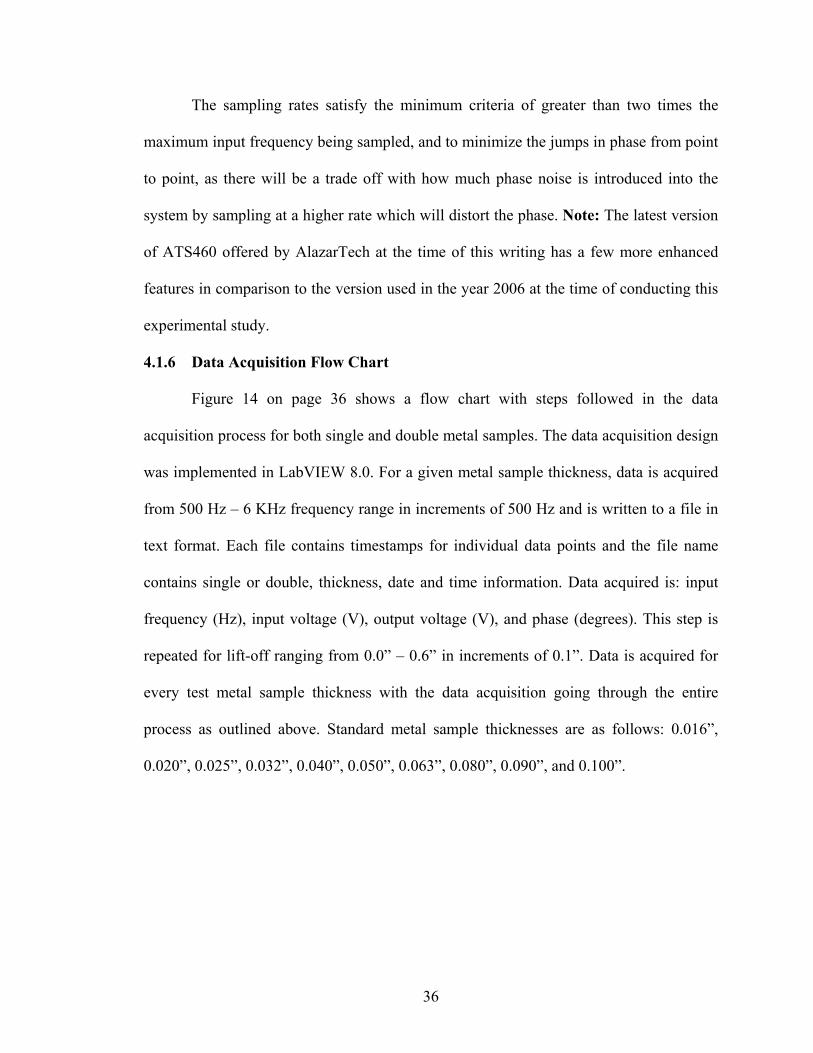
4.1.6 Data Acquis
Figure 14 on page 36 shows
tion process for both single and double metal samples. The data acquisition design
was implemented in LabVIEW 8.0. For a given metal sample thickness, data is acquired
from 500 Hz – 6 KHz frequency range in increments of 500 Hz and is written to a file in
text format. Each file contains timestamps for individual data points and the file name
contains single or double, thickness, date and time information. Data acquired is: input
frequency (Hz), input voltage (V), output voltage (V), and phase (degrees). This step is
repeated for lift-off ranging from 0.0” – 0.6” in increments of 0.1”. Data is acquired for
every test metal sample thickness with the data acquisition going through the entire
process as outlined above. Standard metal sample thicknesses are as follows: 0.016”,
0.020”, 0.025”, 0.032”, 0.040”, 0.050”, 0.063”, 0.080”, 0.090”, and 0.100”.
36
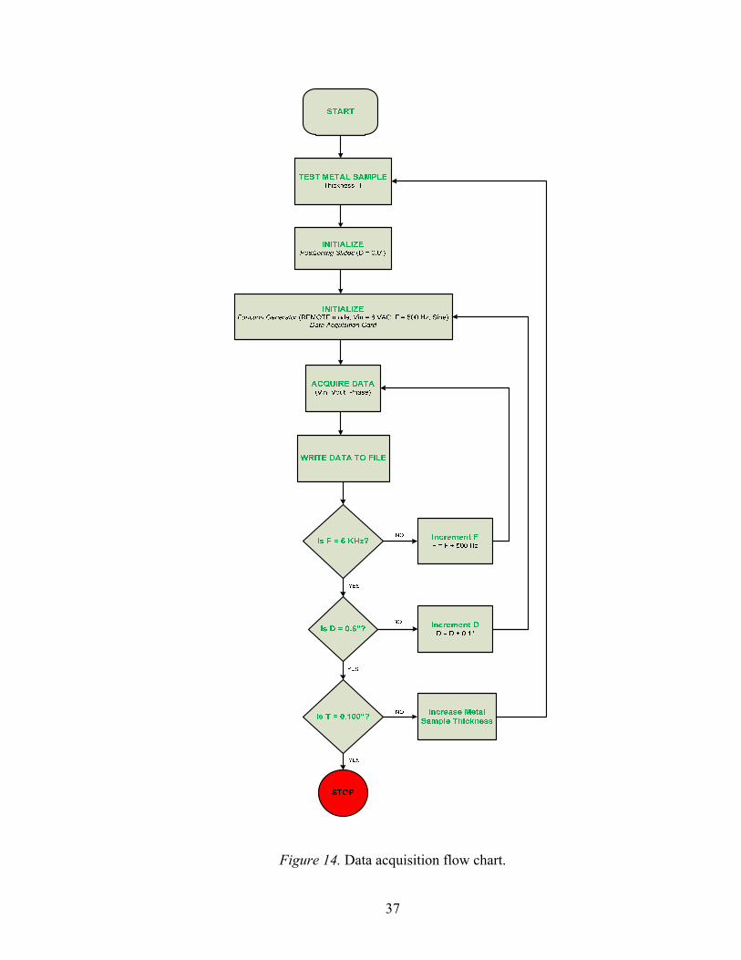
Figure 14. Data acquisition flow chart.
37
4.1.7 Feature Extraction & Characterization Algorithms
The data acquisition design implemented in LabVIEW 8.0 also includes
algorithms to extract the output voltage and phase information. Figure 15 below shows a
simple algorithm used to extract the output AC voltage minus any DC offset existing in
the measured signal. The resultant output voltage signal is thus purely AC in nature.
AC/DCEstimator
-
O/P Measured AC Signal
DC
O/P Voltage Voin volts
Figure 15. Amplitude algorithm.
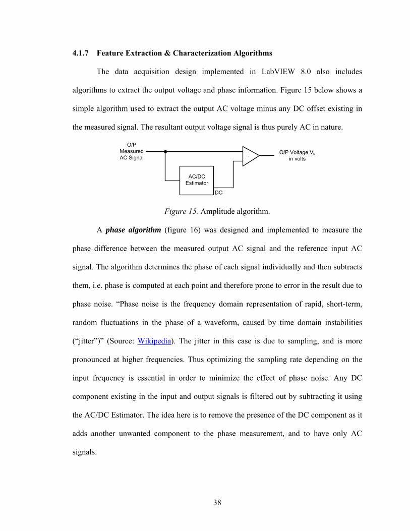
A phase algorithm (figure 16) was designed and implemented to measure the
phase difference between the measured output AC signal and the reference input AC
signal. The algorithm determines the phase of each signal individually and then subtracts
them, i.e. phase is computed at each point and therefore prone to error in the result due to
phase noise. “Phase noise is the frequency domain representation of rapid, short-term,
random fluctuations in the phase of a waveform, caused by time domain instabilities
(“jitter”)” (Source: Wikipedia). The jitter in this case is due to sampling, and is more
pronounced at higher frequencies. Thus optimizing the sampling rate depending on the
input frequency is essential in order to minimize the effect of phase noise. Any DC
component existing in the input and output signals is filtered out by subtracting it using
the AC/DC Estimator. The idea here is to remove the presence of the DC component as it
adds another unwanted component to the phase measurement, and to have only AC
signals.
38
Figure 16. Phase algorithm.
“The Hilbert transform is a linear operator which takes a function, u(t), and
produces a function, H(u)(t), with the same domain” (Source: Wikipedia). “x = hilbert(xr)
returns a complex helical sequence, sometimes called the analytic signal, from a real data
sequence. The analytic signal x = xr + j*xi has a real part, xr, which is the original data,
and an imaginary part, xi, which contains the Hilbert transform. The imaginary part is a
version of the original real sequence with a 90° phase shift. Sines are therefore
transformed to cosines and vice versa. The Hilbert transformed series has the same
amplitude and frequency content as the original real data and includes phase information
that depends on the phase of the original data” (Source: The MathWorks, Inc.).
Further, to make the DC offset zero, whole number of cycles is acquired thus
making the Hilbert transform more accurate across the whole waveform. There will be
less error at the beginning and end (variation) of the final phase difference result. Next,
the resultant complex signals are converted to polar form in order to extract the phase
information. The phase signals are then unwrapped to eliminate discontinuities whose
absolute values exceed pi radians. The unwrapped input and output signals are subtracted
to determine the phase difference between them, which in turn is fed into a polar to
complex function (r = constant 1) and then into a complex to polar function to obtain the
39
phase difference in the range of -180 (-pi) to +180 (+pi) radians. Finally, radians are
converted to degrees to compute the phase difference in degrees.
4.1.8 Data Processing, Analysis & Results
Raw data acquired during the data acquisition process is saved in “text” formatted
files. A Windows dynamic link library (DLL) is designed and implemented in Microsoft®
Visual Basic 6.0. The executable DLL reads raw data from each text file and outputs
input reference voltage in volts, output measured voltage in volts and the phase difference
in degrees that is in turn written to a text file for further analysis. Two text files are
created one each for ‘Single’ and ‘Double’. DLL implementation in Visual Basic is not
straight forward as in other programming applications, but code design and
implementation is much faster and easier in Visual Basic. In order to implement a DLL in
Visual Basic, wrapper (proxy) executables for the C2.exe and LINK.exe executables files
need to be created and then linked to the corresponding original executables. A detailed
explanation on the procedure to be followed is explained by Ron Petrusha [14].
Embedded within the DLL is Visual Basic code to compute the phase difference
between the input and output signals by matching timestamps of individual data points as
the phase algorithm computes the phase at each point and so it is much easier for error to
creep into it since phase is much more sensitive to noise. This code reads in phase data
for both input and output signals from a user specified data file that contains 2000 data
points each. Phase data is parsed and stored in arrays. Next data in the arrays is matched
as closely as possible using timestamp information and any large fluctuations is identified
and eliminated before further processing. These fluctuations are usually noise data and
the amount of acceptable deviation (tolerance) from the actual phase data is user
40
41
specified in the code. Noise corrected data is used to compute the phase difference and
averaged. The final result accounts for the correct phase polarity before being displayed
on a GUI and written to a file. Appendix B provides the Visual Basic code written for
phase computation. The final two text files with processed data for Single and Double
metal samples respectively is used to perform 2D analysis in Microsoft® Excel and
graphical results are obtained for proximity and thickness (single/double) estimation.
Chapter 5
Results
In this chapter, a discussion of the experimental results for proximity and
thickness estimation is presented. Proximity (lift-off or distance between the sensor and
metal sample under test) information is obtained from the output voltage of the sensor,
and thickness information (single or double) is obtained from the phase difference of the
sensors’ output signal with reference to its input signal. “Single” refers to one metal sheet
of a given thickness, and “Double” refers to two metal sheets of identical thickness in a
stacked configuration.
5.1 Proximity Estimation using Output Voltage
For proximity estimation, sensor output voltage is plotted versus multiple
frequencies for a given thickness (single and double) of the metal sample and lift-off
distances varying from 0.0” (sensor flush on the metal sample) to 0.6” in increments of
0.1”. Frequency range of interest is from 500 Hz to 6 KHz in increments of 500 Hz. In
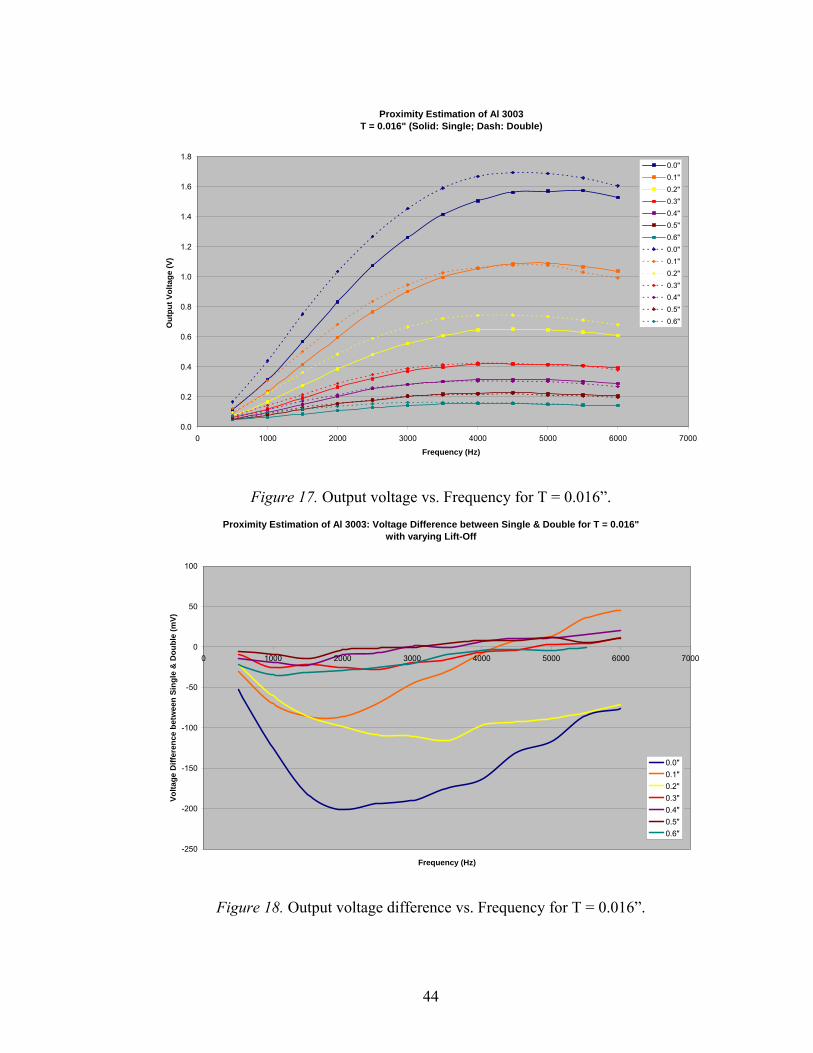
general, as can be seen in figures 17-36 below, proximity information can be obtained at
frequencies greater than 2 KHz and this minimum frequency tends higher as lift-off
distance and thickness increase. In the plots below, solid lines indicate ‘single’, and dash
lines indicate ‘double’. Each set of plots for a given thickness of Al 3003 metal sample
consists of output voltage vs. frequency, and voltage difference between single and
42
double vs. frequency. As observed in the output voltage plots, an initial increase in output
voltage amplitude is followed by a decreasing trend as frequency increases. This trend is
caused due to an increasing back EMF, as eddy currents increase with increasing metal
thickness (as long as metal thickness < skin depth). The net result is an increase in output
voltage.
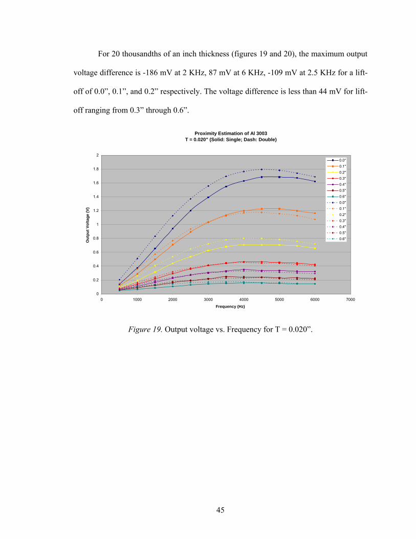
Considering an Al 3003 sample with a thickness of 16 thousandths of an inch
(figures 17 and 18), proximity can be clearly estimated at 0.0”, 0.1” and 0.2” as the
maximum output voltage difference between single and double is -201 mV at 2 KHz, -86
mV at 2 KHz, and -115 mV at 3.5 KHz respectively. Negative voltage difference
indicates the output voltage for a single sheet is less than double and positive voltage
difference indicates the output voltage for a single sheet is greater than double. The
output voltage difference is less than 35 mV from 0.3” through 0.6”. As the skin depth or
standard depth of penetration decreases at higher frequencies, it is observed that the
output voltage difference has zero crossings at higher frequencies as the lift-off increases.
Depending on the end application of the sensor, a minimum threshold for voltage
difference needs to be set (in software) for accurate proximity estimation for a given
thickness. As an example if we consider 50 mV as the minimum voltage, the threshold
condition is satisfied at a frequency range of 500 Hz to 6 KHz at 0.0”, 750 Hz to 3 KHz
at 0.1”, and 1 KHz to 6 KHz at 0.2”; thus proximity for a 0.016” thick metal sample
(single or double) can be estimated at 0.0”, 0.1” and 0.2” in the indicated frequency range
respectively. This threshold is not met for a lift-off of 0.3” through 0.6”. Similar
observations for proximity estimation are made for the other Al 3003 alloy metal sample
thicknesses.
43
Proximity Estimation of Al 3003T = 0.016" (Solid: Single; Dash: Double)
0.0
0.2
0.4
0.6
0.8
1.0
1.2
1.4
1.6
1.8
0 1000 2000 3000 4000 5000 6000 7000
Frequency (Hz)
Out
put V
olta
ge (V
)0.0"0.1"0.2"0.3"0.4"0.5"0.6"0.0"0.1"0.2"0.3"0.4"0.5"0.6"
Figure 17. Output voltage vs. Frequency for T = 0.016”. Proximity Estimation of Al 3003: Voltage Difference between Single & Double for T = 0.016"
with varying Lift-Off
-250
-200
-150
-100
-50
0
50
100
0 1000 2000 3000 4000 5000 6000 7000
Frequency (Hz)
Volta
ge D
iffer
ence
bet
wee
n Si
ngle
& D
oubl
e (m
V)
0.0"0.1"0.2"0.3"0.4"0.5"0.6"
Figure 18. Output voltage difference vs. Frequency for T = 0.016”.
44
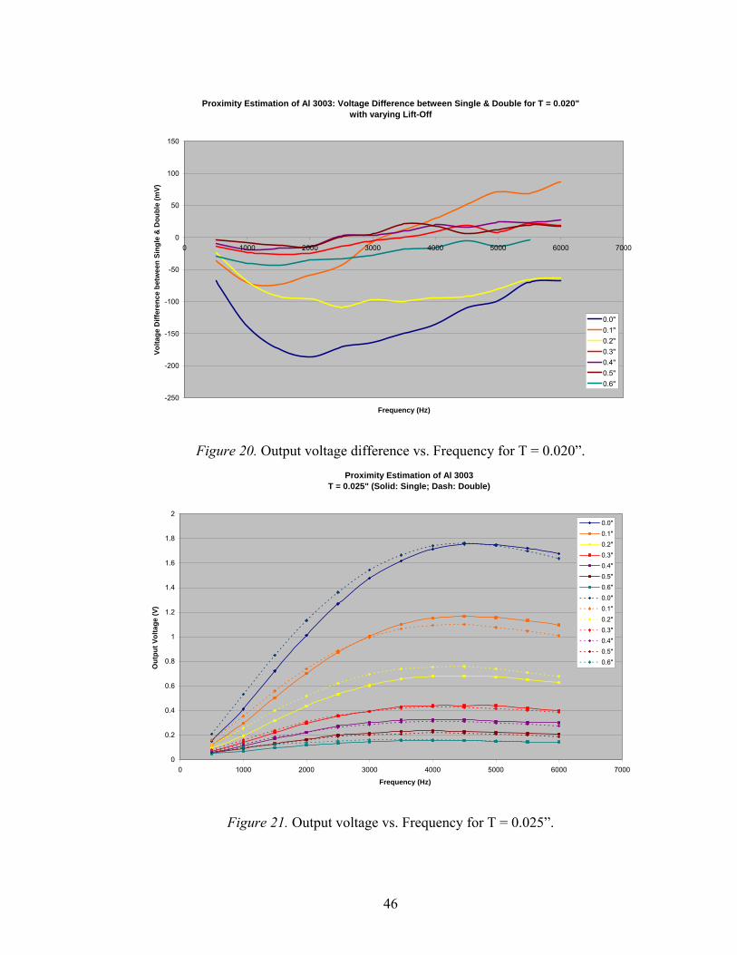
For 20 thousandths of an inch thickness (figures 19 and 20), the maximum output
voltage difference is -186 mV at 2 KHz, 87 mV at 6 KHz, -109 mV at 2.5 KHz for a lift-
off of 0.0”, 0.1”, and 0.2” respectively. The voltage difference is less than 44 mV for lift-
off ranging from 0.3” through 0.6”.
Proximity Estimation of Al 3003T = 0.020" (Solid: Single; Dash: Double)
0
0.2
0.4
0.6
0.8
1
1.2
1.4
1.6
1.8
2
0 1000 2000 3000 4000 5000 6000 7000
Frequency (Hz)
Out
put V
olta
ge (V
)
0.0"0.1"0.2"0.3"0.4"0.5"0.6"0.0"0.1"0.2"0.3"0.4"0.5"0.6"
Figure 19. Output voltage vs. Frequency for T = 0.020”.
45
Proximity Estimation of Al 3003: Voltage Difference between Single & Double for T = 0.020" with varying Lift-Off
-250
-200
-150
-100
-50
0
50
100
150
0 1000 2000 3000 4000 5000 6000 7000
Frequency (Hz)
Volta
ge D
iffer
ence
bet
wee
n Si
ngle
& D
oubl
e (m
V)
0.0"0.1"0.2"0.3"0.4"0.5"0.6"
Figure 20. Output voltage difference vs. Frequency for T = 0.020”. Proximity Estimation of Al 3003
T = 0.025" (Solid: Single; Dash: Double)
0
0.2
0.4
0.6
0.8
1
1.2
1.4
1.6
1.8
2
0 1000 2000 3000 4000 5000 6000 7000
Frequency (Hz)
Out
put V
olta
ge (V
)
0.0"0.1"0.2"0.3"0.4"0.5"0.6"0.0"0.1"0.2"0.3"0.4"0.5"0.6"
Figure 21. Output voltage vs. Frequency for T = 0.025”.
46
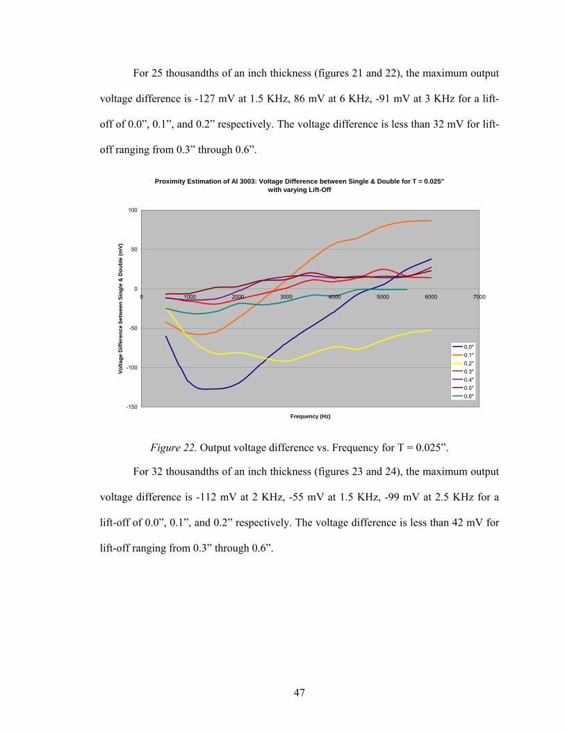
For 25 thousandths of an inch thickness (figures 21 and 22), the maximum output
voltage difference is -127 mV at 1.5 KHz, 86 mV at 6 KHz, -91 mV at 3 KHz for a lift-
off of 0.0”, 0.1”, and 0.2” respectively. The voltage difference is less than 32 mV for lift-
off ranging from 0.3” through 0.6”.
Proximity Estimation of Al 3003: Voltage Difference between Single & Double for T = 0.025" with varying Lift-Off
-150
-100
-50
0
50
100
0 1000 2000 3000 4000 5000 6000 7000
Frequency (Hz)
Volta
ge D
iffer
ence
bet
wee
n Si
ngle
& D
oubl
e (m
V)
0.0"0.1"0.2"0.3"0.4"0.5"0.6"
Figure 22. Output voltage difference vs. Frequency for T = 0.025”.
For 32 thousandths of an inch thickness (figures 23 and 24), the maximum output
voltage difference is -112 mV at 2 KHz, -55 mV at 1.5 KHz, -99 mV at 2.5 KHz for a
lift-off of 0.0”, 0.1”, and 0.2” respectively. The voltage difference is less than 42 mV for
lift-off ranging from 0.3” through 0.6”.
47
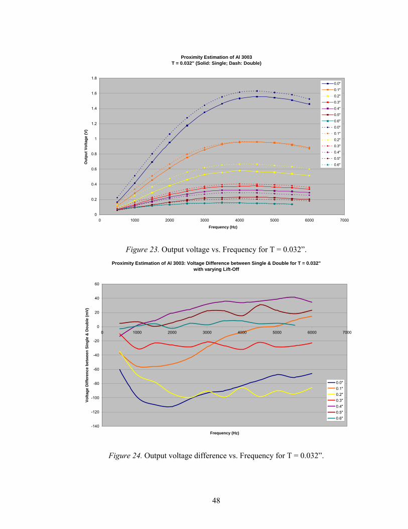
Proximity Estimation of Al 3003T = 0.032" (Solid: Single; Dash: Double)
0
0.2
0.4
0.6
0.8
1
1.2
1.4
1.6
1.8
0 1000 2000 3000 4000 5000 6000 7000
Frequency (Hz)
Out
put V
olta
ge (V
)0.0"
0.1"
0.2"
0.3"
0.4"
0.5"
0.6"
0.0"
0.1"
0.2"
0.3"
0.4"
0.5"
0.6"
Figure 23. Output voltage vs. Frequency for T = 0.032”. Proximity Estimation of Al 3003: Voltage Difference between Single & Double for T = 0.032"
with varying Lift-Off
-140
-120
-100
-80
-60
-40
-20
0
20
40
60
0 1000 2000 3000 4000 5000 6000 7
Frequency (Hz)
Volta
ge D
iffer
ence
bet
wee
n Si
ngle
& D
oubl
e (m
V)
000
0.0"0.1"0.2"0.3"0.4"0.5"0.6"
Figure 24. Output voltage difference vs. Frequency for T = 0.032”.
48

For 40 thousandths of an inch thickness (figures 25 and 26), the maximum output
voltage difference is 88 mV at 6 KHz, 75 mV at 5 KHz, -57 mV at 1.5 KHz for a lift-off
of 0.0”, 0.1”, and 0.2” respectively. The voltage difference is less than 34 mV for lift-off
ranging from 0.3” through 0.6”.
Proximity Estimation of Al 3003T = 0.040" (Solid: Single; Dash: Double)
0
0.2
0.4
0.6
0.8
1
1.2
1.4
1.6
1.8
2
0 1000 2000 3000 4000 5000 6000 7000
Frequency (Hz)
Out
put V
olta
ge (V
)
0.0"0.1"0.2"0.3"0.4"0.5"0.6"0.0"0.1"0.2"0.3"0.4"0.5"0.6"
Figure 25. Output voltage vs. Frequency for T = 0.040”.
49
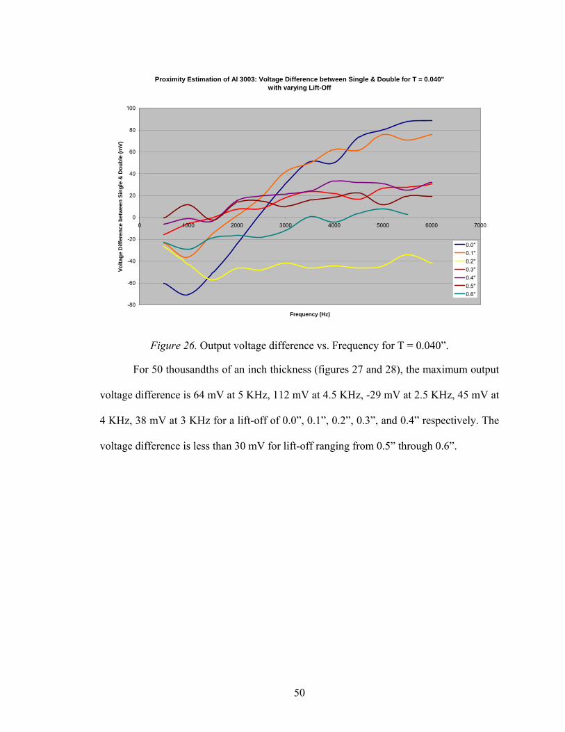
Proximity Estimation of Al 3003: Voltage Difference between Single & Double for T = 0.040" with varying Lift-Off
-80
-60
-40
-20
0
20
40
60
80
100
0 1000 2000 3000 4000 5000 6000 7000
Frequency (Hz)
Volta
ge D
iffer
ence
bet
wee
n Si
ngle
& D
oubl
e (m
V)
0.0"0.1"0.2"0.3"0.4"0.5"0.6"
Figure 26. Output voltage difference vs. Frequency for T = 0.040”.
For 50 thousandths of an inch thickness (figures 27 and 28), the maximum output
voltage difference is 64 mV at 5 KHz, 112 mV at 4.5 KHz, -29 mV at 2.5 KHz, 45 mV at
4 KHz, 38 mV at 3 KHz for a lift-off of 0.0”, 0.1”, 0.2”, 0.3”, and 0.4” respectively. The
voltage difference is less than 30 mV for lift-off ranging from 0.5” through 0.6”.
50
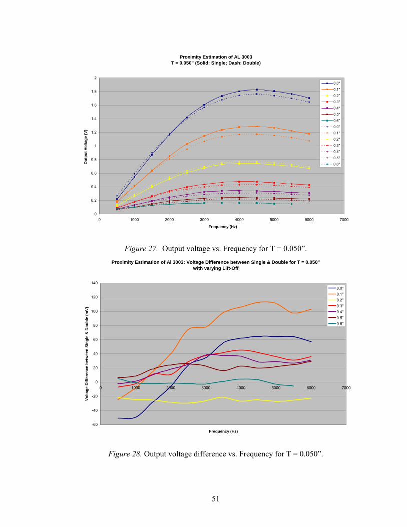
Proximity Estimation of AL 3003T = 0.050" (Solid: Single; Dash: Double)
0
0.2
0.4
0.6
0.8
1
1.2
1.4
1.6
1.8
2
0 1000 2000 3000 4000 5000 6000 7000
Frequency (Hz)
Out
put V
olta
ge (V
)0.0"
0.1"
0.2"
0.3"
0.4"
0.5"
0.6"
0.0"
0.1"
0.2"
0.3"
0.4"
0.5"
0.6"
Figure 27. Output voltage vs. Frequency for T = 0.050”. Proximity Estimation of Al 3003: Voltage Difference between Single & Double for T = 0.050"
with varying Lift-Off
-60
-40
-20
0
20
40
60
80
100
120
140
0 1000 2000 3000 4000 5000 6000 7000
Frequency (Hz)
Volta
ge D
iffer
ence
bet
wee
n Si
ngle
& D
oubl
e (m
V)
0.0"0.1"0.2"0.3"0.4"0.5"0.6"
Figure 28. Output voltage difference vs. Frequency for T = 0.050”.
51

For 63 thousandths of an inch thickness (figures 29 and 30), the maximum output
voltage difference is 214 mV at 4.5 KHz, 76 mV at 5.5 KHz, -44 mV at 4.5 KHz for a
lift-off of 0.0”, 0.1”, and 0.2” respectively. The voltage difference is less than 41 mV for
lift-off ranging from 0.3” through 0.6”.
Proximity Estimation of Al 3003T = 0.063" (Solid: Single; Dash: Double)
0
0.2
0.4
0.6
0.8
1
1.2
1.4
1.6
1.8
2
0 1000 2000 3000 4000 5000 6000 7000
Frequency (Hz)
Out
put V
olta
ge (V
)
0.0"0.1"0.2"0.3"0.4"0.5"0.6"0.0"0.1"0.2"0.3"0.4"0.5"0.6"
Figure 29. Output voltage vs. Frequency for T = 0.063”.
52
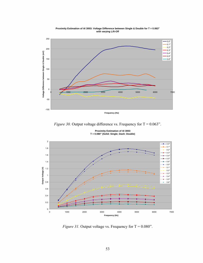
Proximity Estimation of Al 3003: Voltage Difference between Single & Double for T = 0.063" with varying Lift-Off
-100
-50
0
50
100
150
200
250
0 1000 2000 3000 4000 5000 6000 7
Frequency (Hz)
Volta
ge D
iffer
ence
bet
wee
n Si
ngle
& D
oubl
e (m
V)
000
0.0"0.1"0.2"0.3"0.4"0.5"0.6"
Figure 30. Output voltage difference vs. Frequency for T = 0.063”. Proximity Estimation of Al 3003
T = 0.080" (Solid: Single; Dash: Double)
0
0.2
0.4
0.6
0.8
1
1.2
1.4
1.6
1.8
2
0 1000 2000 3000 4000 5000 6000 7000
Frequency (Hz)
Out
put V
olta
ge (V
)
0.0"0.1"0.2"0.3"0.4"0.5"0.6"0.0"0.1"0.2"0.3"0.4"0.5"0.6"
Figure 31. Output voltage vs. Frequency for T = 0.080”.
53
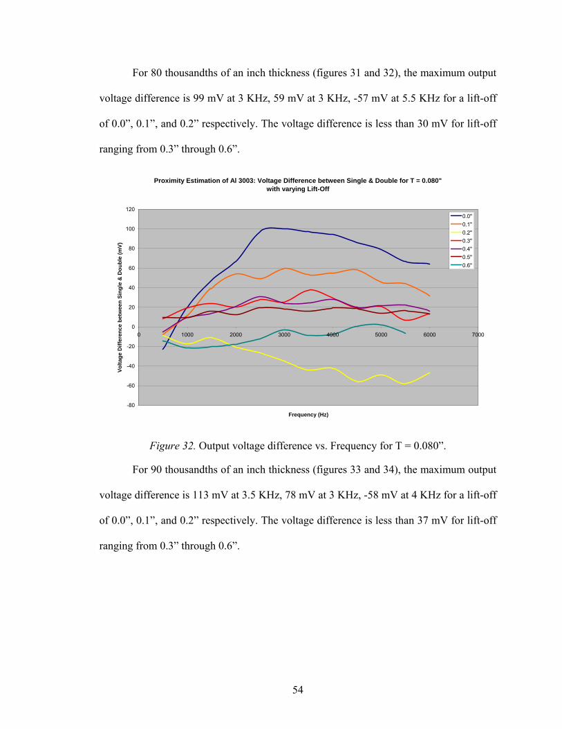
For 80 thousandths of an inch thickness (figures 31 and 32), the maximum output
voltage difference is 99 mV at 3 KHz, 59 mV at 3 KHz, -57 mV at 5.5 KHz for a lift-off
of 0.0”, 0.1”, and 0.2” respectively. The voltage difference is less than 30 mV for lift-off
ranging from 0.3” through 0.6”.
Proximity Estimation of Al 3003: Voltage Difference between Single & Double for T = 0.080" with varying Lift-Off
-80
-60
-40
-20
0
20
40
60
80
100
120
0 1000 2000 3000 4000 5000 6000 7000
Frequency (Hz)
Volta
ge D
iffer
ence
bet
wee
n Si
ngle
& D
oubl
e (m
V)
0.0"0.1"0.2"0.3"0.4"0.5"0.6"
Figure 32. Output voltage difference vs. Frequency for T = 0.080”.
For 90 thousandths of an inch thickness (figures 33 and 34), the maximum output
voltage difference is 113 mV at 3.5 KHz, 78 mV at 3 KHz, -58 mV at 4 KHz for a lift-off
of 0.0”, 0.1”, and 0.2” respectively. The voltage difference is less than 37 mV for lift-off
ranging from 0.3” through 0.6”.
54
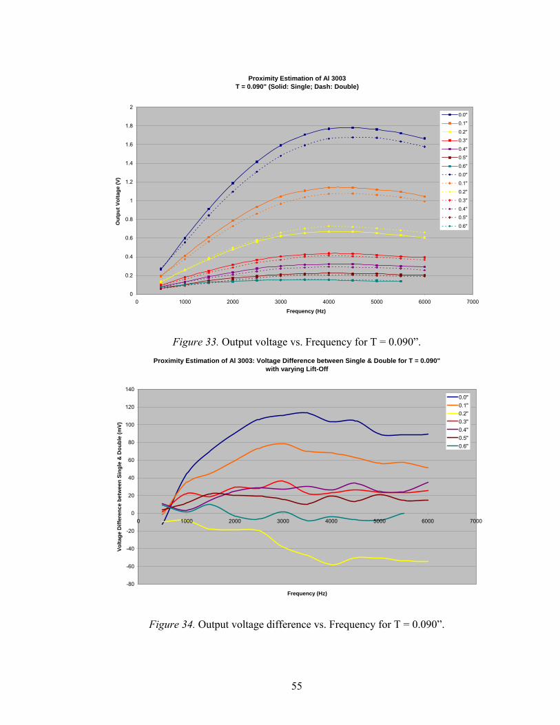
Proximity Estimation of Al 3003T = 0.090" (Solid: Single; Dash: Double)
0
0.2
0.4
0.6
0.8
1
1.2
1.4
1.6
1.8
2
0 1000 2000 3000 4000 5000 6000 7000
Frequency (Hz)
Out
put V
olta
ge (V
)0.0"
0.1"
0.2"
0.3"
0.4"
0.5"
0.6"
0.0"
0.1"
0.2"
0.3"
0.4"
0.5"
0.6"
Figure 33. Output voltage vs. Frequency for T = 0.090”. Proximity Estimation of Al 3003: Voltage Difference between Single & Double for T = 0.090"
with varying Lift-Off
-80
-60
-40
-20
0
20
40
60
80
100
120
140
0 1000 2000 3000 4000 5000 6000 7000
Frequency (Hz)
Volta
ge D
iffer
ence
bet
wee
n Si
ngle
& D
oubl
e (m
V)
0.0"0.1"0.2"0.3"0.4"0.5"0.6"
Figure 34. Output voltage difference vs. Frequency for T = 0.090”.
55
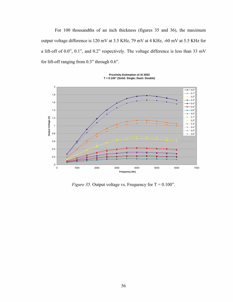
For 100 thousandths of an inch thickness (figures 35 and 36), the maximum
output voltage difference is 120 mV at 3.5 KHz, 79 mV at 4 KHz, -60 mV at 5.5 KHz for
a lift-off of 0.0”, 0.1”, and 0.2” respectively. The voltage difference is less than 33 mV
for lift-off ranging from 0.3” through 0.6”.
Proximity Estimation of Al 3003T = 0.100" (Solid: Single; Dash: Double)
0
0.2
0.4
0.6
0.8
1
1.2
1.4
1.6
1.8
2
0 1000 2000 3000 4000 5000 6000 7000
Frequency (Hz)
Out
put V
olta
ge (V
)
0.0"0.1"0.2"0.3"0.4"0.5"0.6"0.0"0.1"0.2"0.3"0.4"0.5"0.6"
Figure 35. Output voltage vs. Frequency for T = 0.100”.
56
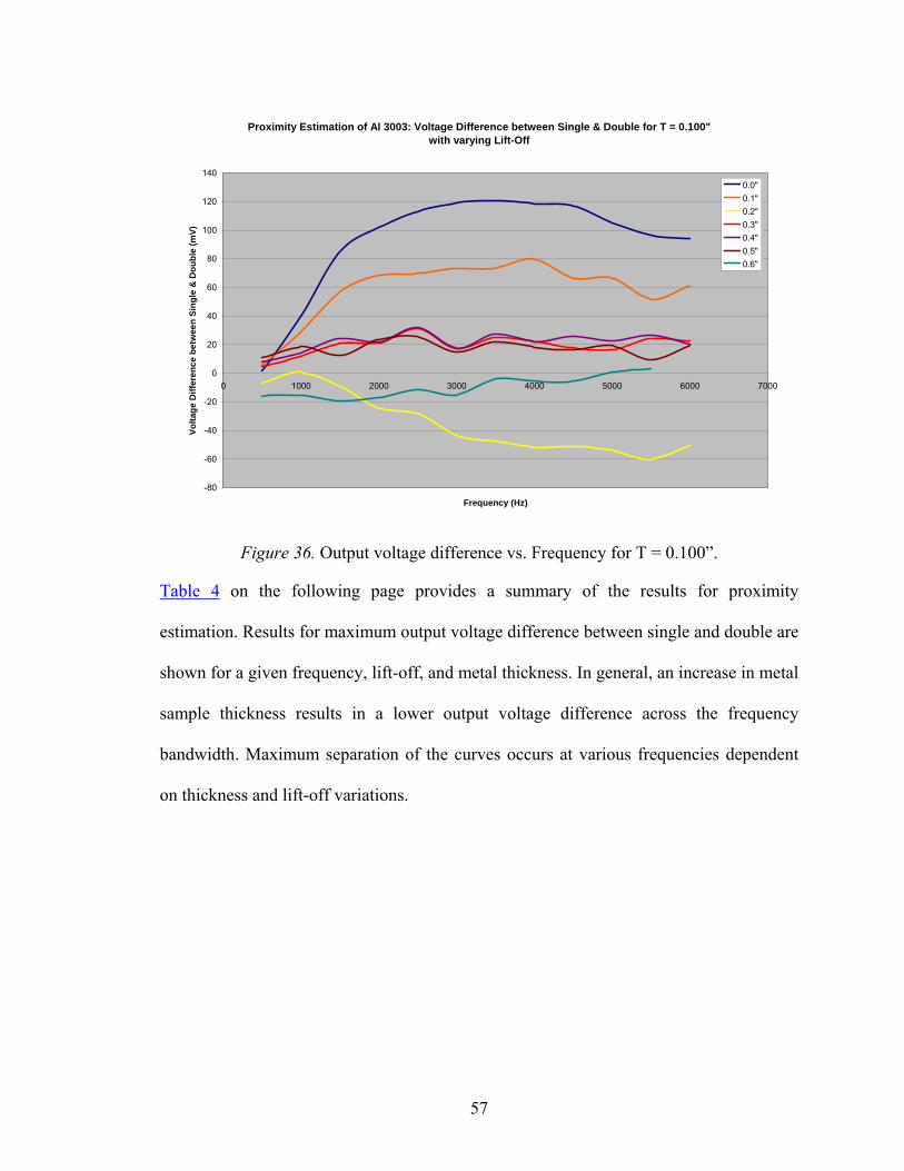
Proximity Estimation of Al 3003: Voltage Difference between Single & Double for T = 0.100" with varying Lift-Off
-80
-60
-40
-20
0
20
40
60
80
100
120
140
0 1000 2000 3000 4000 5000 6000 7000
Frequency (Hz)
Volta
ge D
iffer
ence
bet
wee
n Si
ngle
& D
oubl
e (m
V)0.0"0.1"0.2"0.3"0.4"0.5"0.6"
Figure 36. Output voltage difference vs. Frequency for T = 0.100”.
Table 4 on the following page provides a summary of the results for proximity
estimation. Results for maximum output voltage difference between single and double are
shown for a given frequency, lift-off, and metal thickness. In general, an increase in metal
sample thickness results in a lower output voltage difference across the frequency
bandwidth. Maximum separation of the curves occurs at various frequencies dependent
on thickness and lift-off variations.
57
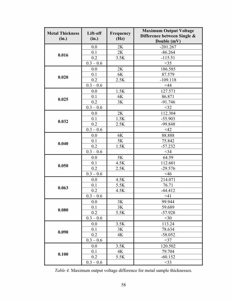
Metal Thickness (in.)
Lift-off (in.)
Frequency (Hz)
Maximum Output Voltage Difference between Single &
Double (mV)
0.016
0.0 2K -201.267 0.1 2K -86.264 0.2 3.5K -115.51
0.3 – 0.6 <35
0.020
0.0 2K 186.585 0.1 6K 87.579 0.2 2.5K -109.118
0.3 – 0.6 <44
0.025
0.0 1.5K 127.571 0.1 6K 86.871 0.2 3K -91.746
0.3 – 0.6 <32
0.032
0.0 2K 112.304 0.1 1.5K -55.903 0.2 2.5K -99.848
0.3 – 0.6 <42
0.040
0.0 6K 88.888 0.1 5K 75.842 0.2 1.5K -57.232
0.3 – 0.6 <34
0.050
0.0 5K 64.59 0.1 4.5K 112.601 0.2 2.5K -29.576
0.3 – 0.6 <46
0.063
0.0 4.5K 214.071 0.1 5.5K 76.71 0.2 4.5K -44.412
0.3 – 0.6 <41
0.080
0.0 3K 99.944 0.1 3K 59.689 0.2 5.5K -57.928
0.3 – 0.6 <30
0.090
0.0 3.5K 113.24 0.1 3K 78.634 0.2 4K -58.052
0.3 – 0.6 <37
0.100
0.0 3.5K 120.502 0.1 4K 79.704 0.2 5.5K -60.152
0.3 – 0.6 <33
Table 4. Maximum output voltage difference for metal sample thicknesses.
58
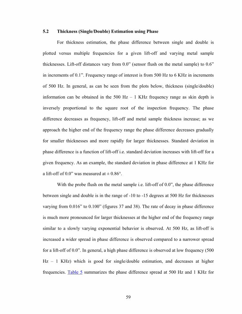
5.2 Thickness (Single/Double) Estimation using Phase
For thickness estimation, the phase difference between single and double is
plotted versus multiple frequencies for a given lift-off and varying metal sample
thicknesses. Lift-off distances vary from 0.0” (sensor flush on the metal sample) to 0.6”
in increments of 0.1”. Frequency range of interest is from 500 Hz to 6 KHz in increments
of 500 Hz. In general, as can be seen from the plots below, thickness (single/double)
information can be obtained in the 500 Hz – 1 KHz frequency range as skin depth is
inversely proportional to the square root of the inspection frequency. The phase
difference decreases as frequency, lift-off and metal sample thickness increase; as we
approach the higher end of the frequency range the phase difference decreases gradually
for smaller thicknesses and more rapidly for larger thicknesses. Standard deviation in
phase difference is a function of lift-off i.e. standard deviation increases with lift-off for a
given frequency. As an example, the standard deviation in phase difference at 1 KHz for
a lift-off of 0.0” was measured at ± 0.86°.
With the probe flush on the metal sample i.e. lift-off of 0.0”, the phase difference
between single and double is in the range of -10 to -15 degrees at 500 Hz for thicknesses
varying from 0.016” to 0.100” (figures 37 and 38). The rate of decay in phase difference
is much more pronounced for larger thicknesses at the higher end of the frequency range
similar to a slowly varying exponential behavior is observed. At 500 Hz, as lift-off is
increased a wider spread in phase difference is observed compared to a narrower spread
for a lift-off of 0.0”. In general, a high phase difference is observed at low frequency (500
Hz – 1 KHz) which is good for single/double estimation, and decreases at higher
frequencies. Table 5 summarizes the phase difference spread at 500 Hz and 1 KHz for
59
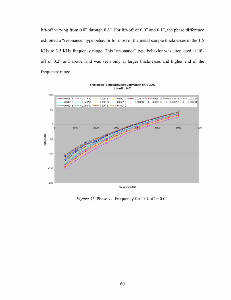
lift-off varying from 0.0” through 0.6”. For lift-off of 0.0” and 0.1”, the phase difference
exhibited a “resonance” type behavior for most of the metal sample thicknesses in the 1.5
KHz to 3.5 KHz frequency range. This “resonance” type behavior was attenuated at lift-
off of 0.2” and above, and was seen only at larger thicknesses and higher end of the
frequency range.
Thickness (Single/Double) Estimation of Al 3003 Lift-off = 0.0"
-200
-150
-100
-50
0
50
100
0 1000 2000 3000 4000 5000 6000 7000
Frequency (Hz)
Phas
e (d
eg)
0.016" S 0.016" D 0.020" S 0.020" D 0.025" S 0.025" D 0.032" S 0.032" D0.040" S 0.040" D 0.050" S 0.050" D 0.063" S 0.063" D 0.080" S 0.080" D0.090" S 0.090" D 0.100" S 0.100" D
Figure 37. Phase vs. Frequency for Lift-off = 0.0”.
60
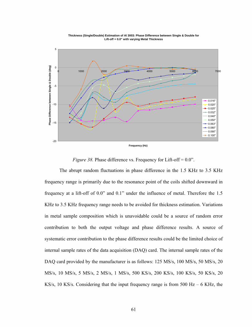
Thickness (Single/Double) Estimation of Al 3003: Phase Difference between Single & Double for Lift-off = 0.0" with varying Metal Thickness
-20
-15
-10
-5
0
5
0 1000 2000 3000 4000 5000 6000 7000
Frequency (Hz)
Phas
e D
iffer
ence
bet
wee
n Si
ngle
& D
oubl
e (d
eg)
0.016"0.020"0.025"0.032"0.040"0.050"0.063"0.080"0.090"0.100"
Figure 38. Phase difference vs. Frequency for Lift-off = 0.0”.
The abrupt random fluctuations in phase difference in the 1.5 KHz to 3.5 KHz
frequency range is primarily due to the resonance point of the coils shifted downward in
frequency at a lift-off of 0.0” and 0.1” under the influence of metal. Therefore the 1.5
KHz to 3.5 KHz frequency range needs to be avoided for thickness estimation. Variations
in metal sample composition which is unavoidable could be a source of random error
contribution to both the output voltage and phase difference results. A source of
systematic error contribution to the phase difference results could be the limited choice of
internal sample rates of the data acquisition (DAQ) card. The internal sample rates of the
DAQ card provided by the manufacturer is as follows: 125 MS/s, 100 MS/s, 50 MS/s, 20
MS/s, 10 MS/s, 5 MS/s, 2 MS/s, 1 MS/s, 500 KS/s, 200 KS/s, 100 KS/s, 50 KS/s, 20
KS/s, 10 KS/s. Considering that the input frequency range is from 500 Hz – 6 KHz, the
61
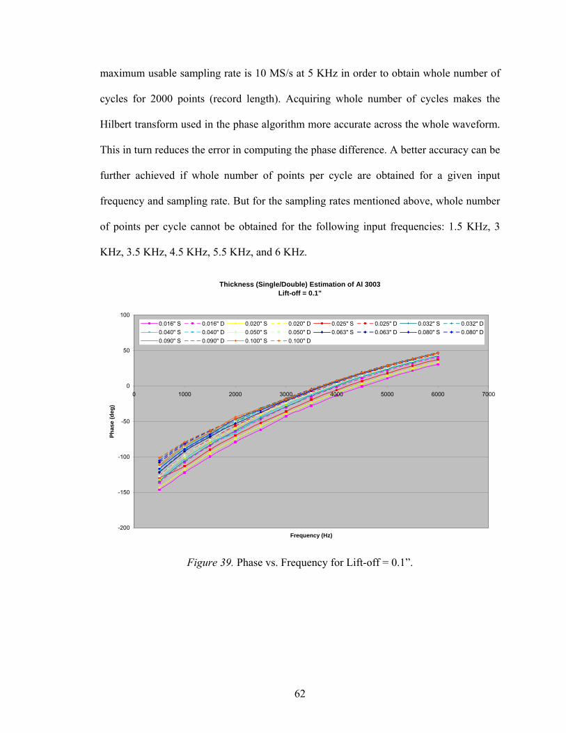
maximum usable sampling rate is 10 MS/s at 5 KHz in order to obtain whole number of
cycles for 2000 points (record length). Acquiring whole number of cycles makes the
Hilbert transform used in the phase algorithm more accurate across the whole waveform.
This in turn reduces the error in computing the phase difference. A better accuracy can be
further achieved if whole number of points per cycle are obtained for a given input
frequency and sampling rate. But for the sampling rates mentioned above, whole number
of points per cycle cannot be obtained for the following input frequencies: 1.5 KHz, 3
KHz, 3.5 KHz, 4.5 KHz, 5.5 KHz, and 6 KHz.
Thickness (Single/Double) Estimation of Al 3003Lift-off = 0.1"
-200
-150
-100
-50
0
50
100
0 1000 2000 3000 4000 5000 6000 7000
Frequency (Hz)
Phas
e (d
eg)
0.016" S 0.016" D 0.020" S 0.020" D 0.025" S 0.025" D 0.032" S 0.032" D0.040" S 0.040" D 0.050" S 0.050" D 0.063" S 0.063" D 0.080" S 0.080" D0.090" S 0.090" D 0.100" S 0.100" D
Figure 39. Phase vs. Frequency for Lift-off = 0.1”.
62
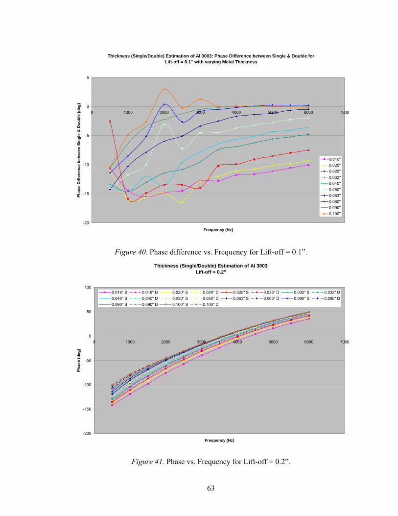
Thickness (Single/Double) Estimation of Al 3003: Phase Difference between Single & Double for Lift-off = 0.1" with varying Metal Thickness
-20
-15
-10
-5
0
5
0 1000 2000 3000 4000 5000 6000 7000
Frequency (Hz)
Phas
e D
iffer
ence
bet
wee
n Si
ngle
& D
oubl
e (d
eg)
0.016"0.020"0.025"0.032"0.040"0.050"0.063"0.080"0.090"0.100"
Figure 40. Phase difference vs. Frequency for Lift-off = 0.1”.
Thickness (Single/Double) Estimation of Al 3003Lift-off = 0.2"
-200
-150
-100
-50
0
50
100
0 1000 2000 3000 4000 5000 6000 7000
Frequency (Hz)
Phas
e (d
eg)
0.016" S 0.016" D 0.020" S 0.020" D 0.025" S 0.025" D 0.032" S 0.032" D0.040" S 0.040" D 0.050" S 0.050" D 0.063" S 0.063" D 0.080" S 0.080" D0.090" S 0.090" D 0.100" S 0.100" D
Figure 41. Phase vs. Frequency for Lift-off = 0.2”.
63
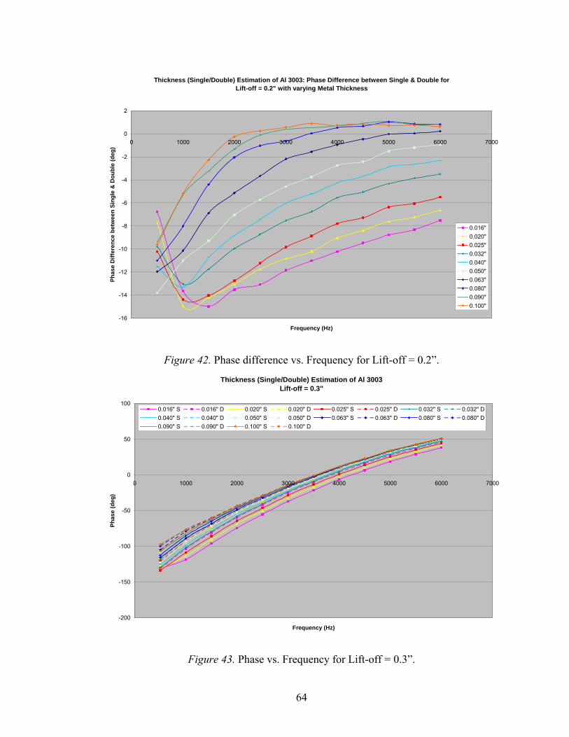
Thickness (Single/Double) Estimation of Al 3003: Phase Difference between Single & Double for Lift-off = 0.2" with varying Metal Thickness
-16
-14
-12
-10
-8
-6
-4
-2
0
2
0 1000 2000 3000 4000 5000 6000 7000
Frequency (Hz)
Phas
e D
iffer
ence
bet
wee
n Si
ngle
& D
oubl
e (d
eg)
0.016"0.020"0.025"0.032"0.040"0.050"0.063"0.080"0.090"0.100"
Figure 42. Phase difference vs. Frequency for Lift-off = 0.2”.
Thickness (Single/Double) Estimation of Al 3003Lift-off = 0.3"
-200
-150
-100
-50
0
50
100
0 1000 2000 3000 4000 5000 6000 7000
Frequency (Hz)
Phas
e (d
eg)
0.016" S 0.016" D 0.020" S 0.020" D 0.025" S 0.025" D 0.032" S 0.032" D0.040" S 0.040" D 0.050" S 0.050" D 0.063" S 0.063" D 0.080" S 0.080" D0.090" S 0.090" D 0.100" S 0.100" D
Figure 43. Phase vs. Frequency for Lift-off = 0.3”.
64
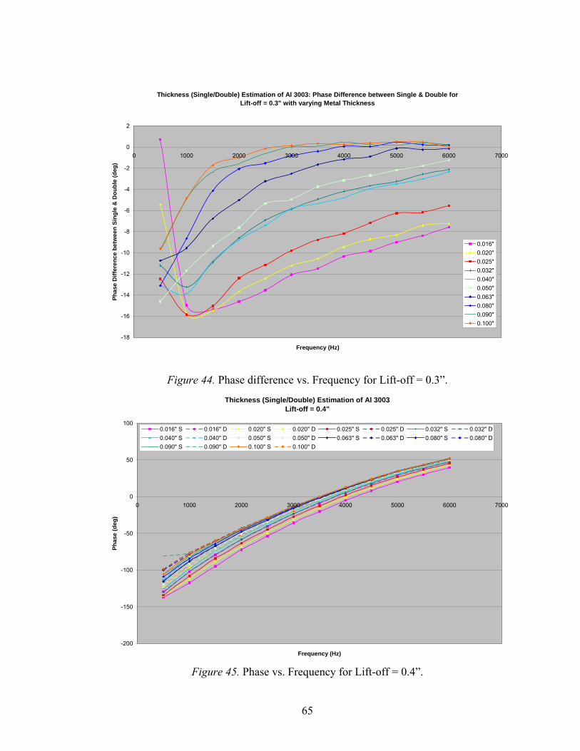
Thickness (Single/Double) Estimation of Al 3003: Phase Difference between Single & Double for
Lift-off = 0.3" with varying Metal Thickness
-18
-16
-14
-12
-10
-8
-6
-4
-2
0
2
0 1000 2000 3000 4000 5000 6000 7000
Frequency (Hz)
Phas
e D
iffer
ence
bet
wee
n Si
ngle
& D
oubl
e (d
eg)
0.016"0.020"0.025"0.032"0.040"0.050"0.063"0.080"0.090"0.100"
Figure 44. Phase difference vs. Frequency for Lift-off = 0.3”.
Thickness (Single/Double) Estimation of Al 3003Lift-off = 0.4"
-200
-150
-100
-50
0
50
100
0 1000 2000 3000 4000 5000 6000 7000
Frequency (Hz)
Phas
e (d
eg)
0.016" S 0.016" D 0.020" S 0.020" D 0.025" S 0.025" D 0.032" S 0.032" D0.040" S 0.040" D 0.050" S 0.050" D 0.063" S 0.063" D 0.080" S 0.080" D0.090" S 0.090" D 0.100" S 0.100" D
Figure 45. Phase vs. Frequency for Lift-off = 0.4”.
65
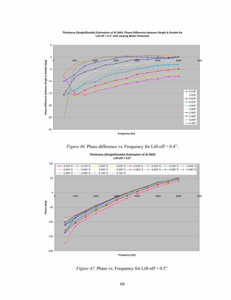
Thickness (Single/Double) Estimation of Al 3003: Phase Difference between Single & Double for Lift-off = 0.4" with varying Metal Thickness
-30
-25
-20
-15
-10
-5
0
5
0 1000 2000 3000 4000 5000 6000 7000
Frequency (Hz)
Phas
e D
iffer
ence
bet
wee
n Si
ngle
& D
oubl
e (d
eg)
0.016"0.020"0.025"0.032"0.040"0.050"0.063"0.080"0.090"0.100"
Figure 46. Phase difference vs. Frequency for Lift-off = 0.4”.
Thickness (Single/Double) Estimation of Al 3003Lift-off = 0.5"
-200
-150
-100
-50
0
50
100
0 1000 2000 3000 4000 5000 6000 7000
Frequency (Hz)
Phas
e (d
eg)
0.016" S 0.016" D 0.020" S 0.020" D 0.025" S 0.025" D 0.032" S 0.032" D0.040" S 0.040" D 0.050" S 0.050" D 0.063" S 0.063" D 0.080" S 0.080" D0.090" S 0.090" D 0.100" S 0.100" D
Figure 47. Phase vs. Frequency for Lift-off = 0.5”.
66
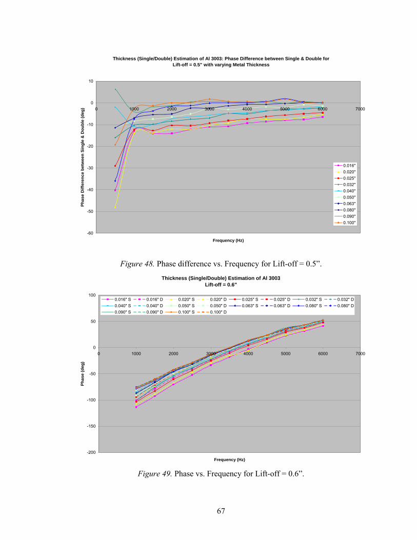
Thickness (Single/Double) Estimation of Al 3003: Phase Difference between Single & Double for Lift-off = 0.5" with varying Metal Thickness
-60
-50
-40
-30
-20
-10
0
10
0 1000 2000 3000 4000 5000 6000 7000
Frequency (Hz)
Phas
e D
iffer
ence
bet
wee
n Si
ngle
& D
oubl
e (d
eg)
0.016"0.020"0.025"0.032"0.040"0.050"0.063"0.080"0.090"0.100"
Figure 48. Phase difference vs. Frequency for Lift-off = 0.5”.
Thickness (Single/Double) Estimation of Al 3003Lift-off = 0.6"
-200
-150
-100
-50
0
50
100
0 1000 2000 3000 4000 5000 6000 7000
Frequency (Hz)
Phas
e (d
eg)
0.016" S 0.016" D 0.020" S 0.020" D 0.025" S 0.025" D 0.032" S 0.032" D0.040" S 0.040" D 0.050" S 0.050" D 0.063" S 0.063" D 0.080" S 0.080" D0.090" S 0.090" D 0.100" S 0.100" D
Figure 49. Phase vs. Frequency for Lift-off = 0.6”.
67
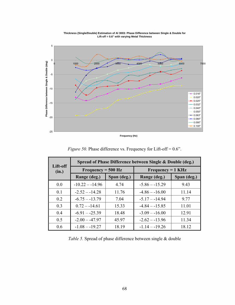
68
Thickness (Single/Double) Estimation of Al 3003: Phase Difference between Single & Double for Lift-off = 0.6" with varying Metal Thickness
-25
-20
-15
-10
-5
0
5
0 1000 2000 3000 4000 5000 6000 7000
Frequency (Hz)
Phas
e D
iffer
ence
bet
wee
n Si
ngle
& D
oubl
e (d
eg)
0.016"0.020"0.025"0.032"0.040"0.050"0.063"0.080"0.090"0.100"
Figure 50. Phase difference vs. Frequency for Lift-off = 0.6”.
Lift-off (in.)
Spread of Phase Difference between Single & Double (deg.)
Frequency = 500 Hz Frequency = 1 KHz Range (deg.) Span (deg.) Range (deg.) Span (deg.)
0.0 -10.22 – -14.96 4.74 -5.86 – -15.29 9.43 0.1 -2.52 – -14.28 11.76 -4.86 – -16.00 11.14 0.2 -6.75 – -13.79 7.04 -5.17 – -14.94 9.77 0.3 0.72 – -14.61 15.33 -4.84 – -15.85 11.01 0.4 -6.91 – -25.39 18.48 -3.09 – -16.00 12.91 0.5 -2.00 – -47.97 45.97 -2.62 – -13.96 11.34 0.6 -1.08 – -19.27 18.19 -1.14 – -19.26 18.12
Table 5. Spread of phase difference between single & double
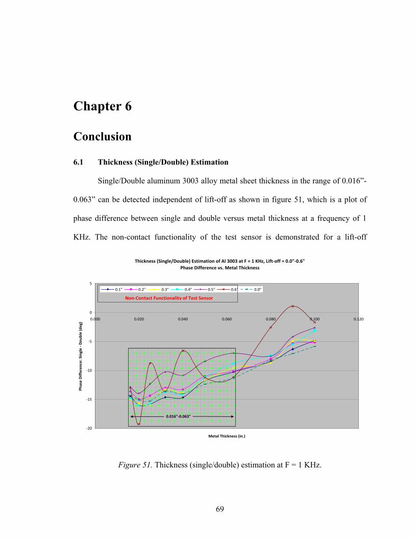
Chapter 6
Conclusion
6.1 Thickness (Single/Double) Estimation
Single/Double aluminum 3003 alloy metal sheet thickness in the range of 0.016”-
0.063” can be detected independent of lift-off as shown in figure 51, which is a plot of
phase difference between single and double versus metal thickness at a frequency of 1
KHz. The non-contact functionality of the test sensor is demonstrated for a lift-off
Thickness (Single/Double) Estimation of Al 3003 at F = 1 KHz, Lift‐off = 0.0"‐0.6"Phase Difference vs. Metal Thickness
‐20
‐15
‐10
‐5
0
5
0.000 0.020 0.040 0.060 0.080 0.100 0.120
Metal Thickness (in.)
Phase Differen
ce: Single ‐ D
ouble (deg)
0.1" 0.2" 0.3" 0.4" 0.5" 0.6" 0.0"
0.016"‐0.063"
Non‐Contact Functionality of Test Sensor
Figure 51. Thickness (single/double) estimation at F = 1 KHz.
69
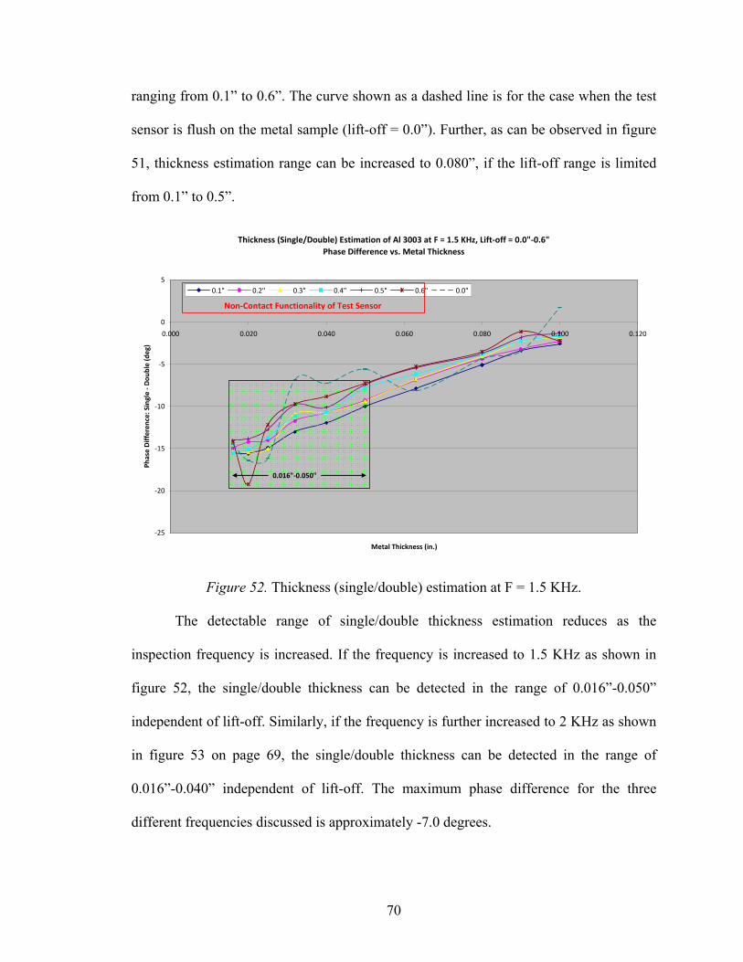
ranging from 0.1” to 0.6”. The curve shown as a dashed line is for the case when the test
sensor is flush on the metal sample (lift-off = 0.0”). Further, as can be observed in figure
51, thickness estimation range can be increased to 0.080”, if the lift-off range is limited
from 0.1” to 0.5”.
Thickness (Single/Double) Estimation of Al 3003 at F = 1.5 KHz, Lift‐off = 0.0"‐0.6"Phase Difference vs. Metal Thickness
‐25
‐20
‐15
‐10
‐5
0
5
0.000 0.020 0.040 0.060 0.080 0.100 0.120
Metal Thickness (in.)
Phase Differen
ce: Single ‐ D
ouble (deg)
0.1" 0.2" 0.3" 0.4" 0.5" 0.6" 0.0"
0.016"‐0.050"
Non‐Contact Functionality of Test Sensor
Figure 52. Thickness (single/double) estimation at F = 1.5 KHz.
The detectable range of single/double thickness estimation reduces as the
inspection frequency is increased. If the frequency is increased to 1.5 KHz as shown in
figure 52, the single/double thickness can be detected in the range of 0.016”-0.050”
independent of lift-off. Similarly, if the frequency is further increased to 2 KHz as shown
in figure 53 on page 69, the single/double thickness can be detected in the range of
0.016”-0.040” independent of lift-off. The maximum phase difference for the three
different frequencies discussed is approximately -7.0 degrees.
70
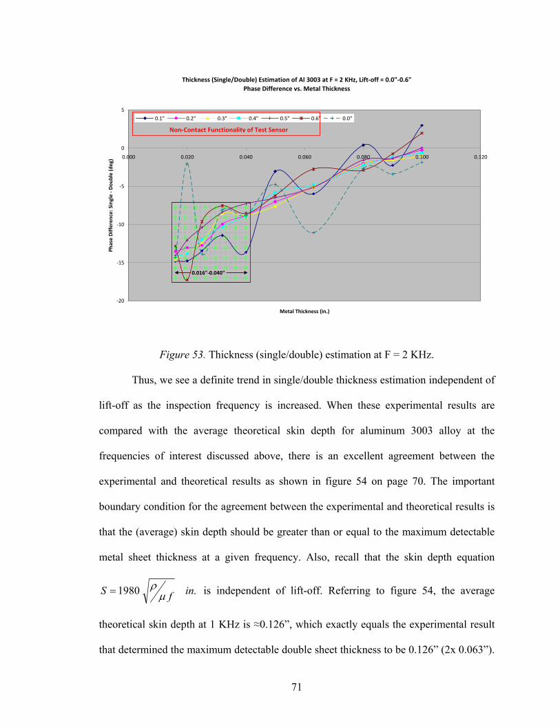
Thickness (Single/Double) Estimation of Al 3003 at F = 2 KHz, Lift‐off = 0.0"‐0.6"Phase Difference vs. Metal Thickness
‐20
‐15
‐10
‐5
0
5
0.000 0.020 0.040 0.060 0.080 0.100 0.120
Metal Thickness (in.)
Phase Differen
ce: Single ‐ D
ouble (deg)
0.1" 0.2" 0.3" 0.4" 0.5" 0.6" 0.0"
0.016"‐0.040"
Non‐Contact Functionality of Test Sensor
Figure 53. Thickness (single/double) estimation at F = 2 KHz.
Thus, we see a definite trend in single/double thickness estimation independent of
lift-off as the inspection frequency is increased. When these experimental results are
compared with the average theoretical skin depth for aluminum 3003 alloy at the
frequencies of interest discussed above, there is an excellent agreement between the
experimental and theoretical results as shown in figure 54 on page 70. The important
boundary condition for the agreement between the experimental and theoretical results is
that the (average) skin depth should be greater than or equal to the maximum detectable
metal sheet thickness at a given frequency. Also, recall that the skin depth equation
.1980 infS μρ= is independent of lift-off. Referring to figure 54, the average
theoretical skin depth at 1 KHz is ≈0.126”, which exactly equals the experimental result
that determined the maximum detectable double sheet thickness to be 0.126” (2x 0.063”).
71
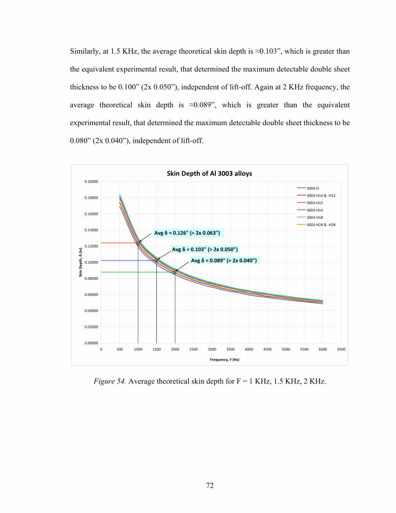
Similarly, at 1.5 KHz, the average theoretical skin depth is ≈0.103”, which is greater than
the equivalent experimental result, that determined the maximum detectable double sheet
thickness to be 0.100” (2x 0.050”), independent of lift-off. Again at 2 KHz frequency, the
average theoretical skin depth is ≈0.089”, which is greater than the equivalent
experimental result, that determined the maximum detectable double sheet thickness to be
0.080” (2x 0.040”), independent of lift-off.
Skin Depth of Al 3003 alloys
0.00000
0.02000
0.04000
0.06000
0.08000
0.10000
0.12000
0.14000
0.16000
0.18000
0.20000
0 500 1000 1500 2000 2500 3000 3500 4000 4500 5000 5500 6000 6500
Frequency, F (Hz)
Skin Dep
th, δ
(in)
3003‐O
3003‐H14 & ‐H12
3003‐H12
3003‐H14
3003‐H18
3003‐H24 & ‐H28
Avg δ ≈ 0.126" (= 2x 0.063")
Avg δ ≈ 0.103" (> 2x 0.050")
Avg δ ≈ 0.089" (> 2x 0.040")
Figure 54. Average theoretical skin depth for F = 1 KHz, 1.5 KHz, 2 KHz.
72
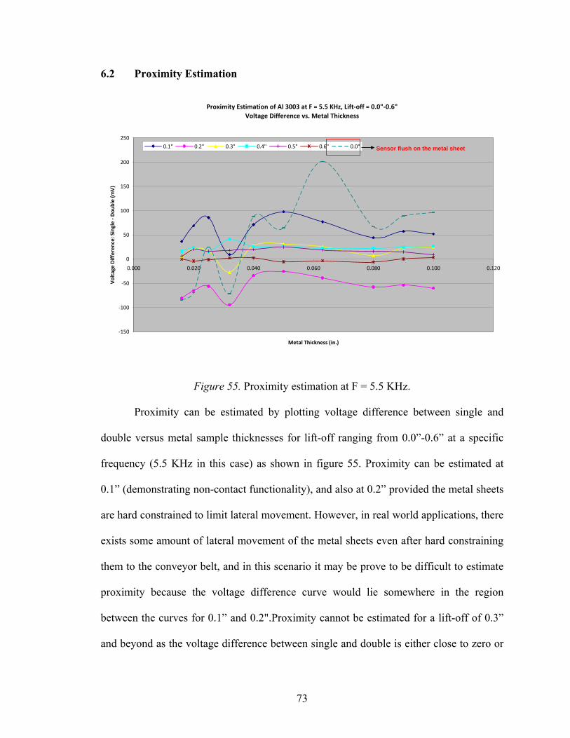
6.2 Proximity Estimation
Proximity Estimation of Al 3003 at F = 5.5 KHz, Lift‐off = 0.0"‐0.6"Voltage Difference vs. Metal Thickness
‐150
‐100
‐50
0
50
100
150
200
250
0.000 0.020 0.040 0.060 0.080 0.100 0.120
Metal Thickness (in.)
Voltage Differen
ce: Single ‐ D
ouble (m
V)
0.1" 0.2" 0.3" 0.4" 0.5" 0.6" 0.0" Sensor flush on the metal sheet
Figure 55. Proximity estimation at F = 5.5 KHz.
Proximity can be estimated by plotting voltage difference between single and
double versus metal sample thicknesses for lift-off ranging from 0.0”-0.6” at a specific
frequency (5.5 KHz in this case) as shown in figure 55. Proximity can be estimated at
0.1” (demonstrating non-contact functionality), and also at 0.2” provided the metal sheets
are hard constrained to limit lateral movement. However, in real world applications, there
exists some amount of lateral movement of the metal sheets even after hard constraining
them to the conveyor belt, and in this scenario it may be prove to be difficult to estimate
proximity because the voltage difference curve would lie somewhere in the region
between the curves for 0.1” and 0.2".Proximity cannot be estimated for a lift-off of 0.3”
and beyond as the voltage difference between single and double is either close to zero or
73
fluctuates between positive and negative regions around zero. Also, when the sensor is
flush on the metal sheet (dashed curve in figure 55), the output voltage difference is
neither completely positive nor negative for smaller thicknesses, and trends into positive
voltage difference territory for metal thicknesses of 0.040” and beyond.
Experimental results have shown feasibility for proximity and thickness
estimation of Al 3003 alloy metal sheets using a single probe dual coil non-contact sensor
based on eddy current technology. Results have shown that proximity estimation requires
sensing at higher frequencies and thickness estimation requires sensing at lower
frequencies as skin depth or standard of penetration is inversely proportional to the
inspection frequency.
6.3 Future Work
• As explained in the “Results” chapter, resonance type behavior was exhibited by
the coils. In the case of output voltage difference, the (yellow) curve for a lift-off
of 0.2” was always negative with no zero crossing or transition point, with the
only exception for a metal thickness of 0.100”. And in the case of phase
difference, abrupt, random fluctuations were seen in the frequency range of 1.5
KHz to 3.5 KHz at a lift-off of 0.0” and 0.1”. In order to better understand this
resonance type behavior, the coils need to be electrical characterized under the
influence of metal sheet thicknesses and variable lift-off to study the effect on coil
impedance and resistance.
• Systematic errors due to environmental effects (EMI, noise, temperature, etc.) can
be minimized by choosing an effective design that meets the housing and
shielding requirements of the sensor for a given application. Another potential
74
75
source of systematic error could be in instrumentation such as the positioning
slides due to incorrect initialization, programmed travel, etc.
• Sensitivity of inductive coils [20] can be increased by using larger diameter coils
(also increases the detectable thickness range), increased number of turns, thinner
copper wire, well compensated differential arrangements for optimal usage of the
dynamic range of sensor electronics, shielding from external noise (EMI) sources.
But the physical size of the coils is often limited by the end application and a
design trade-off between sensor performance and size needs to be achieved.
• Experimenting with different types of bridge circuits for differential impedance
measurement that is less sensitive to variations in lift-off.
• Experimenting with other coil modes of operation (absolute, differential, hybrid,
etc.) in order to achieve greater depth of penetration.
• Experimenting with phase algorithms for extracting a more accurate phase
signature for a given metal type. Accuracy of the phase algorithm proposed in this
thesis can be improved by normalizing the input and output signals before Hilbert
transformation if the phase of the respective signals is constant over the entire
cycle. Optimizing sampling rates to minimize phase noise.
• Proximity and thickness estimation of other nonmagnetic metals such as stainless
steel 303 and 304 series.
References
[1] Fraden, J. Handbook of Modern Sensors – Physics, Designs and Applications, 2nd
Ed.; Springer-Verlag, New York, Inc., 1996.
[2] Hellier, C. J. Handbook of Nondestructive Evaluation; McGraw-Hill, New York,
2001.
[3] Kaufman, M., Seidman, A. H. & Sheneman, P. J. Handbook for Electronics
Engineering Technicians, 2nd Ed.; McGraw-Hill, New York, 1984.
[4] Griffiths, D. J. Introduction to Electrodynamics, 3rd Ed.; Prentice-Hall, Inc.,
Upper Saddle River, NJ, 1999.
[5] Bray, D. E. & Stanley, R. K. Nondestructive Evaluation – A Tool in Design,
Manufacturing and Service, Rev. Ed.; CRC Press, Boca Raton, FL, 1997.
[6] American Society for Metals (Corporate Author) Metals Handbook Desk Edition,
2nd Ed.; CRC Press, Boca Raton, FL, 1998.
[7] Tegopoulos, J. A. & Kriezis, E. E. Eddy Currents in Linear Conducting Media –
Studies in Electrical and Electronic Engineering, Vol. 16; Elsevier Science
Publishers B. V., The Netherlands, 1985.
[8] Jackson, J. D. Classical Electrodynamics, 3rd Ed.; John Wiley & Sons, Inc.,
Hoboken, NJ, 1999.
[9] Proakis, J. G. & Manolakis, D. G. Introduction to Digital Signal Processing;
Macmillan Publishing Company, New York, NY, 1988.
76
[10] Kaiser, C. J. The Inductor Handbook, 1st Ed.; CJ Publishing, Olathe, KS, 1997.
[11] Allocca, J. A. & Stuart, A. Transducers – Theory and Applications; Reston
Publishing Company, Inc., Reston, VA, 1984.
[12] McLyman, Colonel W. T. Transformer and Inductor Design Handbook, 2nd Rev.
Ed.; Marcel Dekker, Inc., New York, NY, 1988.
[13] Balena, F. Programming Microsoft Visual Basic 6.0; Microsoft Press, Redmond,
WA, 1999.
[14] Petrusha, R. Creating a Windows DLL with Visual Basic; 2005.
http://windowsdevcenter.com/pub/a/windows/2005/04/26/create_dll.html?page=1
[15] C. V. Dodd and W. E. Deeds, “Analytical Solutions to Eddy-Current Probe-Coil
Problems” J. Appl. Phys., vol. 39, no. 6, pp. 2829–2839, May 1968.
[16] W. Yin, R. Binns, S. J. Dickinson, C. Davis and A. J. Peyton, “Analysis of the
Liftoff Effect of Phase Spectra for Eddy Current Sensors” IEEE Transactions on
Instrumentation and Measurement, vol. 56, no. 6, pp. 2775-2781, December 2007.
[17] W. Yin and A. J. Peyton, “Thickness Measurement of Metallic Plates With an
Electromagnetic Sensor Using Phase Signature Analysis” IEEE Transactions on
Instrumentation and Measurement, vol. 57, no. 8, pp. 1803-1807, August 2008.
[18] D. Placko, H. Clergeot and E. Santander “Industrial Eddy Current Sensors for
Touchless Thickness Measurement” Industry Applications Society Annual
Meeting, vol. 2, pp. 1487-1492, 1989.
[19] B. Wincheski, J. Fulton, S. Nath and M. Namkung “New Eddy Current Probe for
Thickness Gauging of Conductive Materials” NASA Langley Research Center
Technical Report, 1993.
77

78
[20] O. Hesse and S. Pankratyev, “Usage of Magnetic Field Sensors for Low
Frequency Eddy Current Testing” Measurement Science Review, vol. 5, sec. 3,
2005.
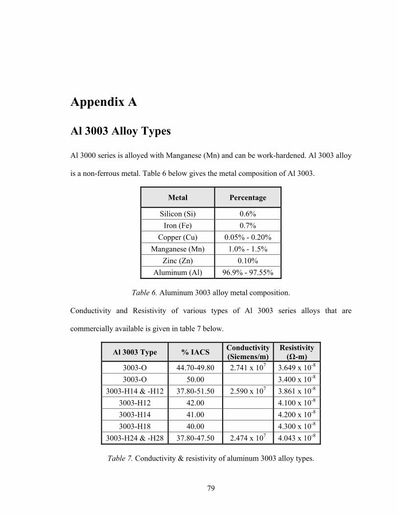
Appendix A
Al 3003 Alloy Types
Al 3000 series is alloyed with Manganese (Mn) and can be work-hardened. Al 3003 alloy
is a non-ferrous metal. Table 6 below gives the metal composition of Al 3003.
Metal Percentage
Silicon (Si) 0.6% Iron (Fe) 0.7%
Copper (Cu) 0.05% - 0.20% Manganese (Mn) 1.0% - 1.5%
Zinc (Zn) 0.10% Aluminum (Al) 96.9% - 97.55%
Table 6. Aluminum 3003 alloy metal composition.
Conductivity and Resistivity of various types of Al 3003 series alloys that are
commercially available is given in table 7 below.
Al 3003 Type % IACS Conductivity (Siemens/m)
Resistivity (Ω-m)
3003-O 44.70-49.80 2.741 x 10⁷ 3.649 x 10⁻⁸ 3003-O 50.00 3.400 x 10⁻⁸
3003-H14 & -H12 37.80-51.50 2.590 x 10⁷ 3.861 x 10⁻⁸ 3003-H12 42.00 4.100 x 10⁻⁸ 3003-H14 41.00 4.200 x 10⁻⁸ 3003-H18 40.00 4.300 x 10⁻⁸
3003-H24 & -H28 37.80-47.50 2.474 x 10⁷ 4.043 x 10⁻⁸
Table 7. Conductivity & resistivity of aluminum 3003 alloy types.
79
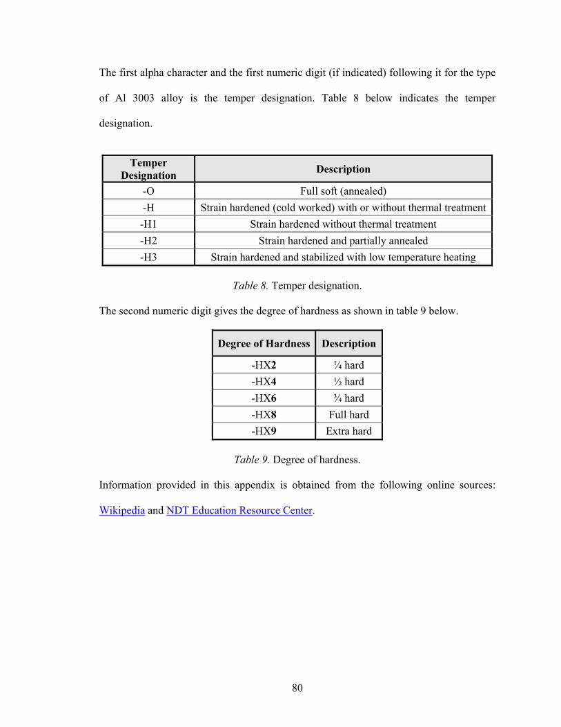
The first alpha character and the first numeric digit (if indicated) following it for the type
of Al 3003 alloy is the temper designation. Table 8 below indicates the temper
designation.
Temper
Designation Description
-O Full soft (annealed) -H Strain hardened (cold worked) with or without thermal treatment-H1 Strain hardened without thermal treatment -H2 Strain hardened and partially annealed -H3 Strain hardened and stabilized with low temperature heating
Table 8. Temper designation.
The second numeric digit gives the degree of hardness as shown in table 9 below.
Degree of Hardness Description
-HX2 ¼ hard -HX4 ½ hard -HX6 ¾ hard -HX8 Full hard -HX9 Extra hard
Table 9. Degree of hardness.
Information provided in this appendix is obtained from the following online sources:
Wikipedia and NDT Education Resource Center.
80

Appendix B Visual Basic Code for Phase Difference Option Explicit ‘ Procedure which computes the phase difference between the I/P and O/P signals Private Sub cmdGo_Click()
Dim filename As String Dim whole_file As String Dim lines() As String Dim one_line() As String Dim num_rows As Long, num_cols As Long Dim phase_data() As String Dim zero_crossing As Double, zero_crossing_in() As Double, zero_crossing_out() As Double Dim R As Long, C As Long Dim sign As Boolean Dim count_in As Integer, count_out As Integer Dim i As Integer, j As Integer, k As Integer Dim temp As Integer, max_temp As Integer Dim lambda() As Double, sum_lambda As Double, avg_lambda As Double Dim delta_size As Integer, delta() As Double, sum_delta As Double, avg_delta As Double Dim phase As Double
‘ Initialize counter variables for 'zero crossing in' and 'zero crossing out' arrays count_in = 0: count_out = 0 ‘ Initialize/Reset all output display boxes to blank txtInput.Text = "" txtOutput.Text = "" lstInputZero.Clear lstOutputZero.Clear txtLambdaSize.Text = "" lstLambda.Clear txtLambdaSum.Text = "" txtLambdaAvg.Text = "" txtDeltaSize.Text = ""
81
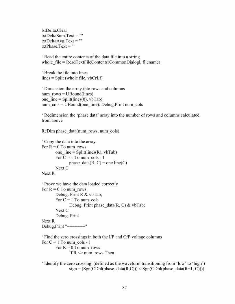
lstDelta.Clear txtDeltaSum.Text = "" txtDeltaAvg.Text = "" txtPhase.Text = "" ‘ Read the entire contents of the data file into a string whole_file = ReadTextFileContents(CommonDialogl, filename) ‘ Break the file into lines lines = Split (whole file, vbCrLf) ‘ Dimension the array into rows and columns num_rows = UBound(lines) one_line = Split(lines(0), vbTab) num_cols = UBound(one_line): Debug.Print num_cols ‘ Redimension the ‘phase data’ array into the number of rows and columns calculated from above ReDim phase_data(num_rows, num_cols) ‘ Copy the data into the array For R = 0 To num_rows
one_line = Split(lines(R), vbTab) For C = 1 To num_cols - 1
phase_data(R, C) = one line(C) Next C
Next R ‘ Prove we have the data loaded correctly For R = 0 To num_rows
Debug. Print R & vbTab; For C = 1 To num_cols
Debug. Print phase_data(R, C) & vbTab; Next C Debug. Print
Next R Debug.Print "=======" ‘ Find the zero crossings in both the I/P and O/P voltage columns For C = 1 To num_cols - 1
For R = 0 To num_rows If R <> num_rows Then
‘ Identify the zero crossing (defined as the waveform transitioning from ‘low’ to ‘high’)
sign = (Sgn(CDbl(phase_data(R,C))) < Sgn(CDbl(phase_data(R+1, C))))
82
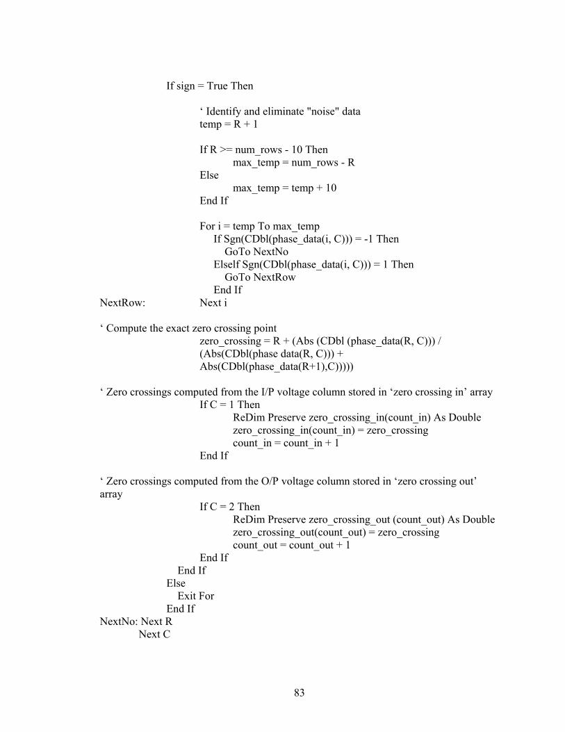
If sign = True Then
‘ Identify and eliminate "noise" data temp = R + 1
If R >= num_rows - 10 Then
max_temp = num_rows - R Else
max_temp = temp + 10 End If
For i = temp To max_temp If Sgn(CDbl(phase_data(i, C))) = -1 Then GoTo NextNo Elself Sgn(CDbl(phase_data(i, C))) = 1 Then GoTo NextRow End If
NextRow: Next i ‘ Compute the exact zero crossing point
zero_crossing = R + (Abs (CDbl (phase_data(R, C))) / (Abs(CDbl(phase data(R, C))) + Abs(CDbl(phase_data(R+1),C)))))
‘ Zero crossings computed from the I/P voltage column stored in ‘zero crossing in’ array If C = 1 Then
ReDim Preserve zero_crossing_in(count_in) As Double zero_crossing_in(count_in) = zero_crossing count_in = count_in + 1
End If ‘ Zero crossings computed from the O/P voltage column stored in ‘zero crossing out’ array
If C = 2 Then ReDim Preserve zero_crossing_out (count_out) As Double
zero_crossing_out(count_out) = zero_crossing count_out = count_out + 1
End If End If Else Exit For End If
NextNo: Next R Next C
83
‘ Output results to form txtlnput.Text = UBound(zero_crossing_in) + 1 txtOutput.Text = UBound(zero_crossing_out) + 1 For i = 0 To UBound(zero_crossing_in)
lstInputZero.AddItem zero_crossing_in(i) Next For i = 0 To UBound(zero_crossing_ out)
lstOutputZero.AddItem zero_crossing_out(i) Next ‘ Compute the wavelength (lambda) of both I/P and O/P signals and find ‘average lambda’ If UBound(zero_crossing_in) = 0 Then
j = 0 ReDim Preserve lambda(j) As Double lambda(j) = zero_crossing_in(j)
Else For j = 0 To UBound(zero_crossing_in) - 1
ReDim Preserve lambda(j) As Double lambda(j) = zero_crossing_in(j + 1) – zero_crossing_in(j)
Next j End If If UBound(zero_crossing_in) = 0 Then j = 0 Else
j = j - 1 End If If UBound(zero_crossing_out) = 0 Then
j = j + 1: k = 0 ReDim Preserve lambda(j) As Double lambda(j) = zero_crossing_out(k)
Else For k = 0 To UBound(zero_crossing_out) - 1
j = j + 1 ReDim Preserve lambda(j) As Double
lambda(j) = zero_crossing_out(k + 1) – zero_crossing_out(k) Next k
End If For i = 0 To UBound(lambda)
sum_lambda = sum_lambda + lambda (i) Next
84

avg_lambda = sum_lambda / (UBound(lambda) + 1) ‘ Output results to form txtLambdaSize.Text = UBound(lambda) + 1 For i = 0 To UBound(lambda)
lstLambda.AddItem lambda (i) Next txtLambdaSum.Text = sum_lambda txtLambdaAvg.Text = avg_lambda ‘ delta - difference between the corresponding zero crossings of the I/P and O/P signals ‘ Determine the size of the 'delta' array If UBound(zero_crossing_out) > UBound(zero_crossing_in) Then
delta_size = UBound(zero_crossing_in) Elself UBound(zero_crossing_out) < UBound(zero_crossing_in) Then
delta_size = UBound(zero_crossing_out) Elself UBound(zero_crossing_out) = UBound(zero_crossing_in) Then delta_size = UBound(zero_crossing_in) - - End If ‘ Compute 'average delta' For i = 0 To delta_size
ReDim Preserve delta (i) As Double delta(i) = zero_crossing_out(i) – zero_crossing_in (i) Next For i = 0 To UBound(delta)
sum_delta = sum_delta + delta(i) Next avg_delta = sum_delta / (UBound(delta) + 1) ‘ Output results to form txtDeltaSize.Text = UBound(delta) + 1 For i = 0 To UBound(delta)
lstDelta.AddItem delta(i) Next txtDeltaSum.Text = sum_delta txtDeltaAvg.Text = avg_delta ‘ Compute the ‘phase shift’ in degrees and account for correct polarity (+/-1) for the phase phase = (avg_delta / avg_lambda) * 360
85
If Abs(phase) > 180 Then If Sgn(phase) = -1 Then
phase = phase + 360 ElseIf Sgn (phase) = 1 Then
phase = phase - 360 End If
End If With txtPhase.Font
.Name = "Arial"
.Bold = True
.Size = 24 End With txtPhase.Text = phase ‘ Function which reads contents from a user selected (Text) file Private Function ReadTextFileContents(CD As CommonDialog, filename As String) As String
Dim fnum As Integer On Error GoTo ExitNow
With CD
.Filter = "All files (*. *) | *. * | Text files | *.txt | LabVIEW Measurement Files | *.lvm" .FilterIndex = 2 .DefaultExt = "txt" .Flags = cdlOFNReadOnly Or cdlOFNFileMustExist Or cdlOFNCreatePrompt Or cdlOFNNoReadOnlyReturn .DialogTitle = "Select a file to read" .filename = filename 'Exit if user presses Cancel. .CancelError = True .ShowOpen
End With ‘ Open file name For Input As fnum. Read the file's contents into the control. fnum = FreeFile() Open filename For Input As #fnum 'Read the entire contents in one single operation. ReadTextFileContents = Input$(LOF(fnum), fnum) Close #fnum ExitNow:
86

87
Private Sub cmdQuit_Click() Unload Me
End Sub