Protocol for in-situ measurement of underwater ... - GOV.UK

Protocol for In-Situ Underwater

Measurement of Explosive

Ordnance Disposal for UXO

Version 2 (September 2020)

Protocol for in-situ measurement of underwater explosions, version 2 1

Protocol for In-Situ Underwater Measurement of Explosive Ordnance Disposal for UXO

Summary

This document provides guidance on best practice for in-situ measurement of underwater sound

generated from underwater explosions undertaken during disposal of unexploded ordnance in the

ocean. In recent years there has been an increasing need to measure and report levels of

underwater sound generated by these explosions, partly driven by the need to conform to

regulatory requirements with regard to assessment of the environmental impact. Attempts to report

measured noise levels are sometimes difficult to compare if different methodologies and acoustic

metrics are used. This good practice guide aims to provide guidance on best practice for

measurement and for reporting the results using common methodology.

The work to prepare this document was funded in the UK by the Department for Business, Energy

and Industrial Strategy through its Offshore Strategic Environmental Assessment programme.

Version 2 September 2020

2 Protocol for in-situ measurement of underwater explosions, version 2

© NPL Management Limited, 2020

National Physical Laboratory Hampton Road, Teddington, Middlesex, TW11 0LW

This work was funded by the UK Government’s Department for Business, Energy and Industrial Strategy (BEIS) through the through its Offshore Energy Strategic

Environmental Assessment programme.


Contents

Glossary ................................................................................................................................................... 5

1. Introduction .................................................................................................................................... 6

1.1 Background ............................................................................................................................. 6

1.2 Background ............................................................................................................................. 6

2. Instrumentation .............................................................................................................................. 7

2.1 General .................................................................................................................................... 7

2.1.1 Hydrophones ................................................................................................................... 8

2.1.2 Amplifiers ........................................................................................................................ 8

2.1.3 Filters ............................................................................................................................... 8

2.1.4 Analogue to Digital Converter (ADC) .............................................................................. 9

2.1.5 Data storage .................................................................................................................... 9

2.2 Key performance of the measuring system ............................................................................ 9

2.2.1 Sensitivity ........................................................................................................................ 9

2.2.2 Sampling Frequency and range ..................................................................................... 10

2.2.3 Directivity ...................................................................................................................... 11

2.2.4 Signal to noise ratio....................................................................................................... 11

2.2.5 System self-noise .......................................................................................................... 11

2.2.6 Dynamic range .............................................................................................................. 11

2.2.7 System Calibration ........................................................................................................ 12

2.2.8 Field calibration checks ................................................................................................. 12

2.2.9 Summary of recommended performance specification ............................................... 12

3. Deployment................................................................................................................................... 14

3.1 Deployment Methodology .................................................................................................... 14

3.1.1 Static Deployment ......................................................................................................... 14

3.1.2 Vessel based deployment ............................................................................................. 14

3.2 Hydrophone Deployment ..................................................................................................... 15

3.2.1 Hydrophone depth ........................................................................................................ 15

3.2.2 Number of hydrophones ............................................................................................... 15

4. Acoustic measurement ................................................................................................................. 15

4.1 General Remarks ................................................................................................................... 15

4.2 Data Sampling ....................................................................................................................... 16

4.3 Recommended measurement locations ............................................................................... 16


4.3.1 Estimation of peak sound pressure at measurement location ..................................... 16

4.3.2 Minimum and maximum range requirement ............................................................... 16

4.3.3 Spatial configuration of measurements ........................................................................ 17

4.3.4 Multiple explosions ....................................................................................................... 18

4.3.5 Additional measurement locations ............................................................................... 19

4.4 Distance measurement ......................................................................................................... 19

4.5 Depth Profile ......................................................................................................................... 20

4.6 Functional Configuration and Testing ................................................................................... 20

4.7 Protection from damage/loss ............................................................................................... 21

5. Data Processing and Acoustic Metrics .......................................................................................... 21

5.1 Conversion to sound pressure .............................................................................................. 21

5.2 Acoustic Metrics .................................................................................................................... 22

5.2.1 Peak sound pressure and peak sound pressure level ................................................... 22

5.2.2 Single pulse sound exposure level (SELsp) ..................................................................... 23

6. Reporting....................................................................................................................................... 24

6.1 General .................................................................................................................................. 24

6.2 Reporting requirement ......................................................................................................... 24

7. References .................................................................................................................................... 25

Appendix A: Modelling of high order detonation ................................................................................. 27

Appendix B: Peak pressure signal processing considerations .............................................................. 29


Glossary

Abbreviation Terms

ADC Analogue to digital converter

BEIS Department for Business, Energy and Industrial Strategy, UK

DAC Digital to analogue converter

dB Decibel, a logarithmic unit expressing the ratio of a quantity relative to a reference value

EOD Explosive ordnance disposal

Hz Hertz, unit of frequency

JNCC Joint Nature Conservation Committee

NMFS National Marine Fisheries Service, USA

NOAA National Oceanic and Atmospheric Admiration, USA

PTS Permanent Threshold Shift

SEL Sound exposure level

SPL Sound pressure level

TTS Temporal Threshold Shift

UXO Unexploded ordnance


1. Introduction

1.1 Background

Unexploded Ordnance (hereafter UXO) in the marine environment constitutes a major

environmental and safety issue. The UXO contamination typically originates from World War I & II

bombing and shelling, defence mining, munitions dumping, coastal defences and anti-submarine

weaponry. These munitions are slowly degrading in the ocean, and there is a risk of spontaneous

detonation.

This presents significant risk to offshore development projects where developers are building

infrastructure directly on the seabed, such as offshore windfarms or oil and gas platforms. As part of

marine licensing, developers are required to identify these munitions and dispose of them. Removal

of large UXOs are often difficult and disposal is typically undertaken through the use of detonation

of the munition. This in turn generates very high amplitude underwater sound which poses

significant risk to the marine wildlife within close proximity of the exercise.

Underwater explosions can produce some of the highest sound pressures of all anthropogenic sound

sources with the potential to cause fatality and auditory damage to animals in the marine

population. The current mitigation measures are based on the JNCC guidelines [JNCC 2010], and

recently revised exposure criteria [e.g. NMFS 2018, Southall et al. 2019] are typically applied to

establish the impact distance at which detonations could cause physical injury as part of the noise

risk assessment. However, estimates of the injury zone can exceed the practical mitigation

prescribed in the mitigation protocol, which raises concern about the effectiveness of current

practice.

In general, underwater explosions create shock waves (sometimes termed “blast waves”) in the

vicinity. These are high-amplitude waves where there is a very fast initial rise time, and whose

propagation is governed by the nonlinear wave equation. However, at the distant measurement

locations where monitoring is typically undertaken, the waves are typically propagating linearly

[Cheong et al 2020].

1.2 Background

This document describes the recommended methodologies, procedures and measurement system

to be used for the measurement of the radiated underwater sound generated during detonation of

UXO. The motivation for undertaking measurement of the sound radiated by the explosion is the

requirement for assessment of impact on aquatic fauna by regulatory frameworks for offshore

development. Collection of data in a common manner also facilitates the filling of current data and

knowledge gaps on direct measurements of underwater noise generated by explosions on the

seabed.

This document aims to provide a generic approach to measurements that can be applied to

regulatory requirements, whilst providing a common approach to help offshore operators and


developers to collect underwater acoustic measurement in order to help the further understanding

of the impact of explosive sounds in the ocean.

This document is suitable for measurement of underwater sound generated during an Explosive

Ordnance Disposal (EOD) operation, commonly undertaken in construction of offshore windfarms,

oil and gas platforms, and construction of other marine renewable energy devices (MREDs). The EOD

may be undertaken by either high order detonation (where a substantial donor charge is used to

detonate and destroy the UXO), or low order detonation where a smaller charge is used to disrupt

and/or consume the UXO. An example of low-order detonation is deflagration [Robinson et al 2020].

This document covers only the measurement of the radiated sound field in shallow water (<100m).

The guidance in this document covers:

• choice of hydrophone and acquisition systems, including calibration requirements;

• deployment techniques;

• minimum requirement for measuring radiated noise from UXO;

• data handling and storage;

• reporting requirement.

The beneficiaries of this work include consultants, offshore developers of marine renewable energy;

regulators wishing to base their requirements on a common scientific foundation; and in general, all

those making in-situ acoustic measurements of underwater explosions. The guidance contained

herein facilitates comparison between measurements of radiated noise from high order detonation

as well as low order detonation from underwater explosion.

2. Instrumentation

2.1 General This section describes the requirement for the measuring instrumentation and specifies the key

performance specifications, system calibration and other data quality measures. The document

provides no recommendation of instrumentation choice to a specific manufacturer or equipment

type. It only aims to provide minimum specifications to the measuring instrumentation to militate

against any bias caused by equipment choice and measurement methods, and ensure consistent

information is collected for all future UXO detonation.

The measuring system generally consists of the following instruments:

- Hydrophone(s)

- Signal conditioning equipment (such as amplifier(s) and filters)

- Signal digitization and data acquisition equipment

- Data storage

The measuring system may consist of individual components as listed above or as an integrated

system such as an autonomous recorder that provides a self-contained recording system powered

by batteries. The amplifier can also be a separate element in the system to allow an adjustable gain,


or it can be an integral part of the hydrophone but without flexibility of a gain adjustment [BS ISO

18406: 2017].

2.1.1 Hydrophones Hydrophones are devices that detect changes in pressure in water. A hydrophone converts these

pressure changes into an electrical voltage signal, which will then be passed on to other components

of the system. Hydrophones used should be calibrated in conformance with a specification standard

describing standardised procedures such as IEC 60565-1:2020, IEC 60565-2: 2019 or ANSI/ASA

S1.20:2012. As far as possible, hydrophone sensitivity should be invariant at the frequency of

interest. The sensitivity is typically expressed in units of V/Pa, or as a sensitivity level in decibels as

dB re 1 V/μPa, at a succession of discrete frequencies, or in the form of a calibration curve [BIAS, NPL

2014].

Note that if extra cable is added to a hydrophone, this reduces the overall sensitivity for

hydrophones without an integral pre-amplifier, however this will not affect the sensitivity of

hydrophones with built in pre-amplifiers. The reduction of sensitivity of the extension cable must be

characterised to correct the data before analysis, such guidance is detailed in [IEC 60565-1:2020].

2.1.2 Amplifiers The role of an amplifier is to increase the amplitude of signals so that the signals can reach levels

appropriate for the next processing stages. The performance is typically expressed as a gain factor,

either in terms of a linear voltage amplitude gain (e.g. “times 10” or “x10”) or in decibels (e.g. 20 dB).

Note that the amplifier gain may not be invariant with frequency, particularly at the extremes of the

operating frequency band. [NPL 2014]

2.1.3 Filters A filter defines a range of frequencies of a signal which can pass through to the rest of the system,

rejecting frequencies outside of this range. Filters are typically known as low pass, high pass or

bandpass depending on their frequency response. Filters serve a number of purposes: (i) to reduce

the influence of very low frequency parasitic signals (a high pass filter designed to cut out

frequencies of less than 10 Hz which can be generated by non-acoustic mechanisms such as surface

motion and flow noise – such filters are commonly incorporated into commercial hydrophones

which have integral preamplifiers); (ii) to provide some signal equalisation across the frequency

range (usually, this involves a high pass filter with a modest slope which is designed to compensate

for the frequency roll-off observed in typical ambient noise spectra, thus avoiding saturation of the

ADC). (iii) to provide an anti-aliasing function (a low pass filter designed to restrict the frequency

content of the signal before digitization to below the Nyquist frequency of the acquisition system); If

any of the above filters are used in the system, their performance needs to be known to correct the

data before analysis [ISO 18406: 2017].

The filter performance is typically expressed as an insertion loss factor, a positive number expressed

either as a linear factor or in decibels [IEC/BS 61260-1:2014]. By definition, a filter response varies

with frequency, and must be characterised over the full operating frequency range of the system.

Note that some commercial hydrophones with integral preamplifiers are designed with a high pass

filter to remove frequencies less than about 10 Hz to minimize influence of very low frequency

parasitic signals typically generated by surface wave motion and flow noise.


2.1.4 Analogue to Digital Converter (ADC) An ADC is used to convert an analogue signal into a digital format to be processed / read by other

components of the system analysing the signal. To characterise the ADC performance, the range

setting (full-scale) and the calibration factor of the ADC must be known. This is often expressed as a

digital sensitivity, which will depend on the digital amplitude output values (counts) of the ADC for a

stated input voltage, and is typically expressed as counts per volt. Note that this is not the same as

the number of bits of the ADC. Alternatively, it can be expressed as a scaling factor, which is more

commonly done when the ADC output file is formatted into a WAV file where the data is scaled

between values of +1 and -1. In this case, the scaling factor represents the number to multiply the

data by to obtain the sound pressure in pascals (and for a scaling to between +/-1, it represents the

maximum sound pressure detectable by the system) [BIAS, NPL 2014].

2.1.5 Data storage Once data is digitized it is saved in the form of digital files for storage. These files are typically

transferred to an electronic storage media such as a computer hard drive or direct to flash memory

which can read directly for post processing.

To avoid degradation of the data quality, data should ideally be recorded in lossless format to ensure

analysis result is representative of the true sound level. If data compression is used (in order to

increase storage capacity and recording duration), the compression technique must be reported,

and compressed data should be recoverable to the uncompressed state to ensure data quality. All

analysis should be carried out on uncompressed data.

In addition, any crucial metadata such as scaling factor, amplifier gains, sampling frequency must

also be reported to aid the interpretation of results. For example, the scaling factor or range setting

of the ADC, or the gains of any amplifiers, the sampling frequency and the resolution [NPL 2014].

It is desirable that such calibration data information be included in a file header or log file so that the

information is kept with the data. Without this information, the data file may essentially appear

“uncalibrated”. Though a number of suitable data formats exist (for example, WAV file format),

there is no standardised format for storing ocean noise data [NPL 2014].

2.2 Key performance of the measuring system The following outlines the key characteristics for the measuring instrumentation and recommended

setting with regards to measurement of underwater explosion.

2.2.1 Sensitivity The sensitivity of the measuring system must be chosen to be an appropriate value for the

amplitude of the sound signal being measured. The system should be specifically chosen to avoid

nonlinearity and system saturation for high amplitude signals. Sound generated by explosion is of

high amplitude when close to the source (with typical peak sound level exceeding 200 dB re 1 μPa

within the first 500 meters), and system saturation can occur when the pressure amplitude exceeds

its dynamic range. Thus, for measurements made close to the source, a relatively low sensitivity

hydrophone and system is recommended (less than -200 re 1V/ μPa for use at a minimum range of 1

km). However, it should be noted that gain settings for many autonomous recorders and

hydrophones with built-in preamplifiers cannot be modified after deployment, thus considerations


must be given to its deployment position in order to avoid unusable data (a high-gain system may

only be suitable for measurement at substantial distance from the source).

It is good practice that the background noise be reported with the results, preferable measured at

the same location of the low sensitivity hydrophone. Note that it is not appropriate to use the low

sensitivity hydrophone and system to take these background noise measurements with good

accuracy. For background noise measurement, a low noise performance and high sensitivity is

generally required to ensure good signal to noise ratio. The recommended system sensitivity level

for background noise measurement is -185 to -165 dB re 1 V/μPa.

For digital systems, the system records the sound as a digital waveform (rather than providing an

analogue voltage output). The calibration of the digitiser (analogue to digital converter) is

incorporated into the overall sensitivity of the whole system including the digitizer. This may be

termed the digital system sensitivity, which is the number of digital counts per unit change in sound

pressure (unit Pa-1). Sometimes, the digital system sensitivity may be represented as a scaling factor

by which the digital waveform values must be multiplied by to obtain pressure values in pascals (this

is equivalent to the reciprocal of the digital system sensitivity).

Note: In general, the measuring system may introduce a phase delay into the measured signal. This may be accounted for

by representing the system sensitivity as a complex valued quantity, the modulus of which represents the magnitude-only

response (and is described by the definition above), and the phase of which describes the phase response of the system.

2.2.2 Sampling Frequency and range The frequency response of the measuring system shall be set to a frequency range sufficient to cover

all frequency components of interest within the measured signals [IEC 60500:2017]. This

requirement applies to the hydrophone or the measuring sensors, data acquisition system and

amplifiers.

For the measurement of underwater explosions, at minimum the system nominal frequency

bandwidth shall cover between 20 Hz – 20 kHz, with a minimum sampling frequency of at least 43.8

kHz (to capture upper band limit of 22.39 kHz for the 20 kHz third-octave band). However, when

selecting a suitable frequency range for the measurements, consideration of the hearing abilities of

the relevant receptors should be given on a case by case basis. Where the hearing response of

relevant marine receptors extends to higher frequencies, the highest frequency of measurement

should ideally be extended so that the sampling frequency is more than twice the value of the

frequency of interest (or higher than the upper bounds of the highest one-third octave band) [ISO

18406:2017, NMFS 2018, Southall et al, 2019]. For example, to capture the typical audible range of

harbour porpoise which extends to 150 kHz, a sample rate of the recording system should be

selected at or above 300 kHz, at twice the frequency of interest.

It is desirable that the system sensitivity be invariant with frequency over the frequency range of

interest to within a tolerance of 2 dB. The measuring system should be calibrated to a traceable

standard as this will allow correction of the variation in the sensitivity of the instrument. [IEC 60565-

1:2020, IEC 60565-2:2019, IEC 60500:2017]


2.2.3 Directivity The hydrophone used must have an omnidirectional response such that its sensitivity is invariant

with the direction of the incoming signal to within a tolerance of 2 dB over the frequency range of

interest.

Omnidirectionality is generally easily achievable below 20 kHz due the small hydrophone size

compared to the acoustic wavelength. However, if the hydrophone is placed close to a physical

structure, the scattered sound may interfere with the direct sound wave and cause enhanced

directionality at high frequency [ISO 18406 2017, Hayman et al 2017, NPL 2014].

2.2.4 Signal to noise ratio Signal to noise ratio is defined as the ratio of the mean squared signal voltage to the mean square

broadband noise voltage. A signal-to-noise ratio of at least 6 dB level difference shall be required for

all measurements (including any background noise measurement).

2.2.5 System self-noise System self-noise is considered to be the noise originating from the hydrophone and recording

system and it is generated in the absence of any signal due to external acoustic stimulus. In order to

achieve acceptable signal to noise ratio, the system self-noise shall be at least 6 dB below the lowest

signal level in the frequency band of interest.

2.2.6 Dynamic range The dynamic range refers to the measuring system’s effective amplitude range over which the

system can faithfully measure the sound pressure. This ranges from the lowest measurable signal

(system self-noise) to the highest amplitude of a signal without distortion. This can be expressed in

decibels representing the difference between the lowest and highest amplitude level of signal.

Sound generated by explosions has high amplitude and can often exceed the dynamic range of the

measuring system and render the measured signal with “truncated peak”, an effect known as

clipping. In order to avoid clipping, consideration must be given to the dynamic range of the digitizer

ADC and the analogue input of the hydrophone. The system dynamic range shall be chosen to be

sufficient to enable the highest expected sound pressure, at the measurement position, to be

recorded faithfully without distortion or saturation caused by the hydrophone, amplifier, and ADC.

The measuring system is required to be linear over the full dynamic range, requiring that the system

sensitivity is constant over the full range of measurable sound pressure. Systems with dynamic

ranges of in excess of 60 dB are preferred for measurement of sound from explosions at ranges of a

few kilometres.

As a minimum data shall be recorded in resolution no less than 16 bit in the analogue to digital

conversion stage, with a nominal given system dynamic range of 96 dB. However, a 24 bit system

with dynamic range of 144 dB is desirable for this type of measurement. The analogue dynamic

range of the hydrophone should be close to the ADC of the instrument chain. Note that the actual

dynamic range is still limited by the system self-noise and the maximum measurable undistorted

sound.


2.2.7 System Calibration The full measuring system shall be calibrated over the full frequency range of interest. [Hayman et al

2017] This includes the hydrophone, amplifier, filter, and analogue to digital converter. It is

preferred that a full laboratory calibration is performed at minimum every 2 years.

The calibration of the hydrophones must be traceable to national or international standards and

conform to IEC 60565 [IEC 60565-1:2020, IEC 60565-2:2019, IEC 60500:2017].

2.2.8 Field calibration checks In-situ field checks should be undertaken before and after each deployment. This can be performed

using two methods

- Hydrophone calibrator, consists of an air pistonphone that generates a known sound

pressure level at a defined frequency inside a coupling chamber into which the hydrophone

is inserted. Note that this method generally provides a field calibration check at only one

frequency (typically 250Hz) but it allows the integrity of the entire system to be checked. [BS

ISO 18406:2017]

- Use of electrical check calibration of the system components. If the hydrophone has an

insert voltage capability, electrical calibration can be performed through signal injection in

order to check the system electrical integrity. However it does not perform an acoustical

check on the hydrophone element. [NPL 2014]

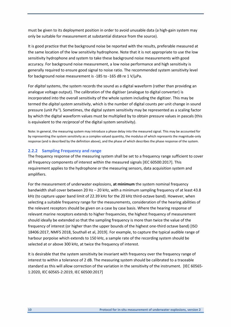
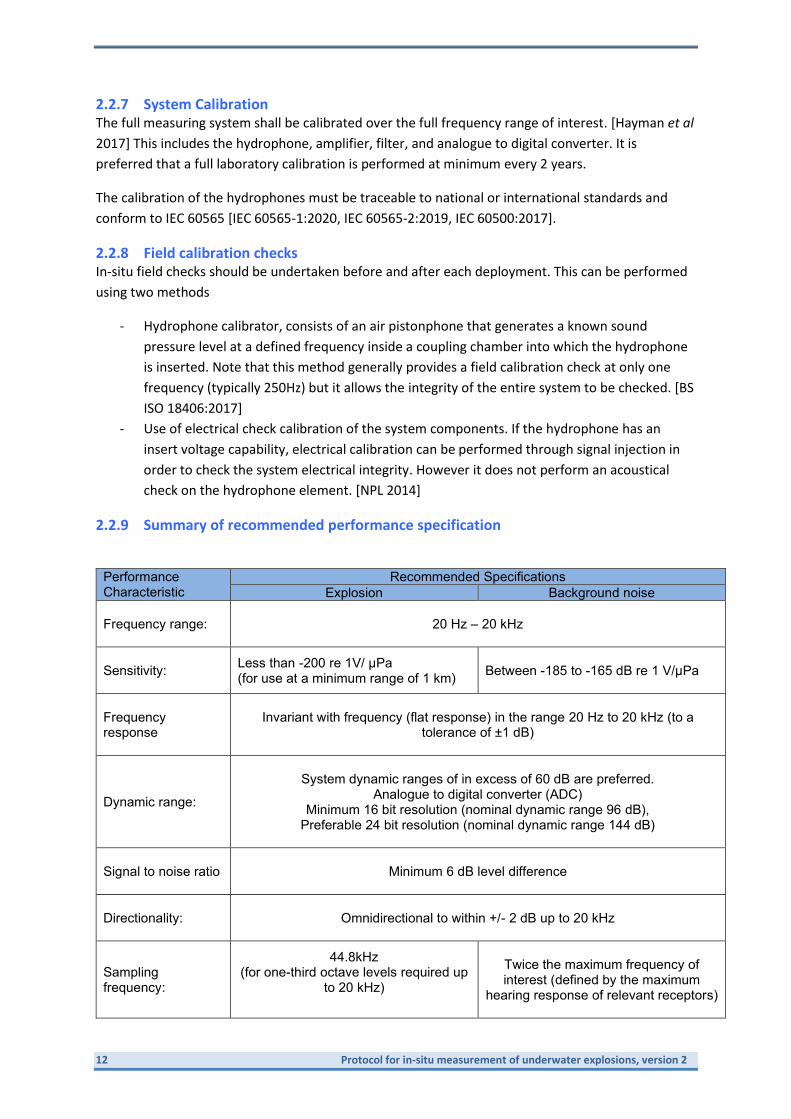
2.2.9 Summary of recommended performance specification

Performance Characteristic

Recommended Specifications

Explosion Background noise

Frequency range:

20 Hz – 20 kHz

Sensitivity:

Less than -200 re 1V/ μPa (for use at a minimum range of 1 km)

Between -185 to -165 dB re 1 V/μPa

Frequency response

Invariant with frequency (flat response) in the range 20 Hz to 20 kHz (to a tolerance of ±1 dB)

Dynamic range:

System dynamic ranges of in excess of 60 dB are preferred.

Analogue to digital converter (ADC) Minimum 16 bit resolution (nominal dynamic range 96 dB),

Preferable 24 bit resolution (nominal dynamic range 144 dB)

Signal to noise ratio

Minimum 6 dB level difference

Directionality:

Omnidirectional to within +/- 2 dB up to 20 kHz

Sampling frequency:

44.8kHz (for one-third octave levels required up

to 20 kHz)

Twice the maximum frequency of interest (defined by the maximum

hearing response of relevant receptors)


Performance Characteristic

Recommended Specifications

Explosion Background noise

Filtering:

Any filter characteristics should be known and corrections applied (low pass and high pass filtering caused by instrumentation). Any low frequency roll-off in

recorder performance due to high pass electronic filtering must be measured so that suitable corrections can be applied.

System self-noise:

Ideally 6 dB below the lowest sound level.

Calibration

Calibrated to traceable standard within the last 2 years

Data storage

Raw data ideally stored in lossless format. Any compression used must be reported, and uncompressed data must be

recoverable before analysis.

Metadata to be stored: instrument calibration and ADC scaling factor, amplifier gains, sampling frequency and resolution


3. Deployment

3.1 Deployment Methodology For measurement of underwater explosions, one or both of the following generic deployment

methods should be adopted depending on available resource and conditions.

3.1.1 Static Deployment A static deployment typically consists of hydrophone(s) connected to an autonomous recorder that

can be moored at the bottom of the seabed to allow remote acoustic measurement in the water

column. This system enables multiple units to be deployed at the same time in order to monitor the

sound propagation at several fixed ranges simultaneously. This is considered a more cost-effective

method for measuring underwater explosions if multiple ranges are required.

With regard to platform noise, a static bottom-mounted deployment is generally preferable to a

surface deployment because the hydrophone is positioned away from the air/water boundary, thus

minimising the effect of this pressure-release boundary on the sound field, and reducing parasitic

signals from the influence of surface wave action. It also has the advantage that measurements may

be safely made at range that is considered unsafe for vessels during a detonation operation.

Field deployment of a static system is typically more complex than a vessel based deployment, as it

requires a mooring to be built and prepared prior to the field trial. Recovery requires either a surface

buoy connected to a seabed anchor or an acoustic release system, which enables the recorder to be

hauled to the surface.

3.1.2 Vessel based deployment This involves deployment of hydrophone (either individually or in arrays) from a vessel, with the

analysis and recording equipment remaining on the vessel, which can be either anchored or drifting.

The method has the advantage that deployment can be quick and mobile, allowing flexibility to suit

different operational changes. The risk of losing instrumentation is low, the data can typically be

monitored as they are acquired and instrument settings can be adjusted in real time to provide the

optimal setting for the required dynamic range to avoid signal saturation.

However, vessel based deployment can suffer from certain types of platform related noise [BS ISO

18406:2017]. As hydrophone is deployed in close proximity with a survey vessel, there is potential

for parasitic signals to be produced. These possible sources of platform noise can include:

1) Flow noise

Low frequency noise caused by the turbulent flow around the hydrophone.

2) Cable strum

Noise caused by the action of current on the taut cable.

3) Surface heave

Large amplitude, low frequency noise caused by the changes of hydrophone depth due

to vertical motion of wave action.

4) Vessel noise

This can be any source of noise originated from survey vessel, it includes the engine

propeller, generator, echo sounder and other vessel machinery.

5) Mechanical noise


This includes any mechanical contacts in close proximity or direct on the hydrophone,

for example mooring anchor chain, direct contact with sediment, or biological abrasion

noise.

6) Electrical noise

This typically caused by measuring system being powered by the vessel electrical main,

causing electrical interference and noise.

Although platform noise is unlikely to mask the high amplitude signal from an explosion for

measurements made close to the source, attempt should be made to minimize its influence and help

improve the data quality for the data analysis. For guidance on how to minimize the above noise

sources, see [BS ISO 18406:2017] and [NPL 2014].

In addition, a human presence is required for a vessel-based deployment, and this may not be

possible if there is a likely encroachment within the safety exclusion zone of the EOD operation.

3.2 Hydrophone Deployment

3.2.1 Hydrophone depth The hydrophone is to be positioned in the lower half of the water depth and at least 2 m above the

seafloor. If hydrophones are to be deployed at two depths, these should be placed in the lower half

of the water column ideally between ½ and ¾ of the total depth, ideally with the separation

between hydrophones maximised.

3.2.2 Number of hydrophones Clearly, one hydrophone at each measurement station is the minimum requirement. However

where feasible, at least two hydrophones are recommended for the respective measuring

location(s). This is to allow redundancy in the measurement and also provide flexibility when

required to use multiple hydrophones of different sensitivity in order to measure high amplitude

sound and low level background noise without signal clipping and distortion. The extra data

collected at the same position also allow the spatial averaging of the acoustic data (assuming data

from all hydrophones are good quality with no clipping) and assist in assessment of measurement

uncertainty.

4. Acoustic measurement

4.1 General Remarks When a UXO is detonated as part of an EOD procedure, it is acknowledged that there is only a single

instantaneous event per detonation, thus repeated measurements as a function of time are not

possible. Spatial sampling is typically limited by health and safety considerations (i.e. measurement

must be clear of any safety exclusion zone) and other operational constraints (i.e. additional

deployment vessel, deployment/recovery time) during the EOD operation. Thus, in this document

emphasis is placed on the far-field sampling of the event to enable comparability of UXO

measurement in a similar setting.


4.2 Data Sampling In general, the measurement shall be chosen to satisfy at least one of the following requirements:

- Measurement at fixed location(s) to monitor the source output for comparison with other

underwater explosion events.

- Measurement to assess the accuracy of predictions made from numerical models.

- Measurement for validation of models of source radiation mechanisms.

- Measurement to derive a source output metric (e.g. a source level)

- Measurement that allow comparison with a normative threshold level (i.e. NMFS guideline

2018)

It is acknowledged that measurements of underwater explosion are site specific and many

parameters cannot be determined, such as the ordnance age, effective charge weight and seabed

properties, etc. The objective is to obtain datasets that are as consistent as possible in order to aid

the understanding of UXO explosion and its impact in the marine environment.

4.3 Recommended measurement locations Recommendations are given according to the different scenarios.

4.3.1 Estimation of peak sound pressure at measurement location UXO found in the open ocean can vary in type and size, and so the distance from the source of the

chosen measurement location must be chosen carefully. It is recommended that before

measurements are undertaken, an estimate is made of the peak sound pressure at the

measurement location generated by the explosion. This estimate should be used to determine the

required measurement system response (in particular, the dynamic range), an appropriate

measurement set up should be chosen that can enable measurements to be carried out without

clipping or saturation of the measured signal at the measurement range.

The peak pressure can be estimated for a given explosive type and location, according to the

following

𝑝𝑝𝑘 = 𝑘 (𝑊

13

𝑅)

𝛼

where ppk = peak sound pressure (MPa) W = charge mass (kg) R = distance from explosion (m) k, α = shock and pressure coefficient The shock and pressure coefficient are derived empirically. Details of the modelling of underwater

explosion and the equivalent coefficients of different explosive type can be found in Appendix A.

4.3.2 Minimum and maximum range requirement The minimum range for measurement is governed by two factors:

• safety considerations requiring all deployments and vessels to be outside the exclusion zone

defined during the EOD operation;


• the dynamic range of the instrumentation used (governing the maximum acoustic signal that

can be faithfully recorded).

The first consideration will determine whether vessel-based deployments are possible in the vicinity

of the EOD operation but may also influence the ability to deploy static systems such as autonomous

recorders. If there are groups of UXO located close together on the seabed, the size of the cluster

may prevent deployments close to any one individual UXO. Ideally, the second consideration should

not be an issue because the system performance may be designed to measure the estimated peak

sound pressure at the location. However, in practice, a limited range of acoustic instrumentation

may be available for use on any deployment, and the maximum recordable sound pressure for the

instrumentation available may influence minimum range achievable.

In consideration of the above issues, the minimum recommended range from the UXO for any

measurement location is 1 km. It is recommended that a measurement is made at 1 km range for all

EOD clearances wherever possible (though it is accepted that there may be some operations where

for reasons of safety or practicality, this may not be possible). In some situations, it may be possible

to deploy a high dynamic range static measuring system closer than 1 km before the EOD operation

begins (assuming there are no issues with vessel manoeuvrability or safety). However, even in such

exceptional circumstances, a measurement should also be made at 1 km.

The measurement is best achieved using a bottom mounted static deployment but a vessel-based

deployment may also be used (Figure 1). A vessel-based deployment at 1 km may be considered

unsafe during the explosive ordnance disposal operation, in which case it is advisory to use static

system deployed in advance of the EOD operation. The recommended 1 km range is based on a far

field shock wave model of a small explosive charge [Aaron 1954], which predicts peak sound

pressure for a given charge of equivalent TNT.

If the recommended range cannot be used due to excessive peak pressure or limitation of measuring

instrumentation, it is acceptable to use an alternative range to ensure the full waveform to be

captured without saturating or distorting the signal, provided requirements described in 2.2.9 can be

satisfied.

The maximum range for a measurement station is recommended to be at least 10 km, and ideally

20 km. However, it is recognised that there may be practical limitations on the maximum range (for

example, where deployments are limited to within the area of a specific offshore development).

4.3.3 Spatial configuration of measurements The minimum number of sampling locations recommended in this document is one single location.

Where operation is restricted by safety constraint and limited resources, this may be the only

option. However, while even one good quality measurement is better than none, it is recommended

that where possible, measurements are made at three or more locations. There are two options for

the spatial configuration of measurement locations.


Measurements along a transect A number of measurement stations are positioned in a straight line along a single azimuthal bearing

from the UXO position, with the closest position no closer than that defined in 4.3.2. Such a strategy

enables the propagation of the acoustic wave along a specified transect to be empirically estimated

by determining the properties of the acoustic pulse as a function of range. It is recommended that (if

possible) ranges are selected by at least an approximate tripling of distance relative to the 1 km

minimum range (for example, say 1 km, 3 km, 10 km, etc.) in order to observe significant changes in

sound pressure over long distances.

Measurements at fixed grid locations (along a variety of bearings) Here, a number of fixed measurement stations are located along a variety of different bearings and

at different ranges from the UXO. This measurement strategy is more suited to an EOD campaign

where numerous UXO are to be cleared from an area, and where re-positioning of the measurement

stations after each EOD clearance is not practical. Here the stations would be positioned on a grid in

the vicinity around the UXO grouping, with the bearings and ranges to the stations varying for each

UXO. The closest position to any UXO should still satisfy the requirements of 4.3.2.

Figure 1 Deployment schematic of hydrophone. (Left) Moored static mooring using an autonomous recorder. (Right) Vessel based deployment. Note: diagram is not to scale.

4.3.4 Multiple explosions In the case of multiple explosive sources closely located, forming an explosive cluster, it may be

possible to position the measuring stations such that the bearings are approximately the same from

the sources to the measuring stations, provided the explosives are close together. This negates the


need to reposition the static deployments in order to satisfy the transect requirement whilst

reducing potential operational errors.

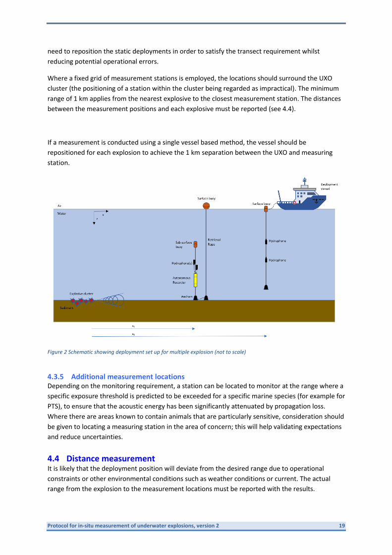
Where a fixed grid of measurement stations is employed, the locations should surround the UXO

cluster (the positioning of a station within the cluster being regarded as impractical). The minimum

range of 1 km applies from the nearest explosive to the closest measurement station. The distances

between the measurement positions and each explosive must be reported (see 4.4).

If a measurement is conducted using a single vessel based method, the vessel should be

repositioned for each explosion to achieve the 1 km separation between the UXO and measuring

station.

Figure 2 Schematic showing deployment set up for multiple explosion (not to scale)

4.3.5 Additional measurement locations Depending on the monitoring requirement, a station can be located to monitor at the range where a

specific exposure threshold is predicted to be exceeded for a specific marine species (for example for

PTS), to ensure that the acoustic energy has been significantly attenuated by propagation loss.

Where there are areas known to contain animals that are particularly sensitive, consideration should

be given to locating a measuring station in the area of concern; this will help validating expectations

and reduce uncertainties.

4.4 Distance measurement It is likely that the deployment position will deviate from the desired range due to operational

constraints or other environmental conditions such as weather conditions or current. The actual

range from the explosion to the measurement locations must be reported with the results.


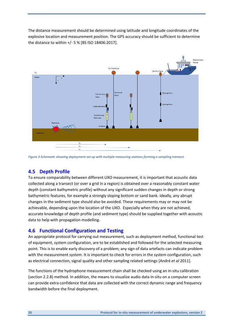
The distance measurement should be determined using latitude and longitude coordinates of the

explosive location and measurement position. The GPS accuracy should be sufficient to determine

the distance to within +/- 5 % [BS ISO 18406:2017].

Figure 3 Schematic showing deployment set up with multiple measuring stations forming a sampling transect.

4.5 Depth Profile To ensure comparability between different UXO measurement, it is important that acoustic data

collected along a transect (or over a grid in a region) is obtained over a reasonably constant water

depth (constant bathymetric profile) without any significant sudden changes in depth or strong

bathymetric features, for example a strongly sloping bottom or sand bank. Ideally, any abrupt

changes in the sediment type should also be avoided. These requirements may or may not be

achievable, depending upon the location of the UXO. Especially when they are not achieved,

accurate knowledge of depth profile (and sediment type) should be supplied together with acoustic

data to help with propagation modelling.

4.6 Functional Configuration and Testing An appropriate protocol for carrying out measurement, such as deployment method, functional test

of equipment, system configuration, are to be established and followed for the selected measuring

point. This is to enable early discovery of a problem; any sign of data artefacts can indicate problem

with the measurement system. It is important to check for errors in the system configuration, such

as electrical connection, signal quality and other sampling related settings [André et al 2011].

The functions of the hydrophone measurement chain shall be checked using an in-situ calibration

(section 2.2.8) method. In addition, the means to visualize audio data in-situ on a computer screen

can provide extra confidence that data are collected with the correct dynamic range and frequency

bandwidth before the final deployment.


It is recommended in-situ calibration checks be carried out on all measurement systems prior of

deployment, and after retrieval of the instrumentation.

4.7 Protection from damage/loss The associated risk of damage is considerable higher when measuring underwater sound from an

UXO. Loss of equipment/data can occur if the final deployment configurations are not selected

carefully [EU TSG Noise 2014b]. This is a problem for all system but autonomous system is especially

more susceptible to damages. The main dangers are potentially caused by the high-amplitude

acoustic wave and excessive vibration acting on the air-filled bodies of many autonomous acoustic

recorders. This can cause damages to the internal component of the recording system if not isolated

properly. If the recorder body is damaged, it can cause water ingress and care should be taken to

design the survey to avoid such damages. An adequate anchor should be used to militate against

movement under the action of currents and withstand the abrupt vibration caused by the blast. The

above damage is more likely for recorders placed very close to the UXO (within the first 2 km).

In addition to loss of equipment, there is also a risk of loss of data. This can result of significant cost

as there is only one opportunity to record the underwater explosion. Vessel based deployment

generally gives the advantage of instantly retrievable data and protects against data loss. However,

for autonomous recorders with archival storage, the data is only available periodically after

recovery. Thus such system must be thoroughly configured and tested (as recommended in section

3.6) before final deployment.

5. Data Processing and Acoustic Metrics

5.1 Conversion to sound pressure The output of the acquisition system of the instrument measurement chain (hydrophone,

preamplifier, ADC) is assumed to be a signal waveform consisting of a digitized time series expressed

in digital counts and representing the signal detected by the hydrophone and recorded by the

acquisition system. The data format is assumed to be a binary data file containing the digitized

signals of the hydrophone recording obtained over a discrete time series, where ti corresponds to

the ith point in the time series.

The data processing to convert the waveform data to sound pressure shall be conducted according

to the following steps.

a) Identify the event in the waveform and read the segment of the data for analysis consisting of N = T fs points where T is the analysis window duration in seconds and fs is the sampling frequency.

b) Confirm that data show no signs of “clipping” (overloading the maximum allowed amplitude of the measurement chain). This will be evident from data samples which reach the maximum or minimum value of the ADC.

c) If required, digital filters may be applied to limit the frequency content of the signal to the overall band of interest and to remove low frequency parasitic signals such as flow noise.


d) Convert the time waveform in the selected widow to a frequency spectrum expressed as frequency bands, either using Fourier analysis or via digital filtering. The frequency bands should be calculated as one-third octave bands.

e) If the system sensitivity is provided in analogue units of V/Pa or dB re 1 V/Pa, then the digitised signal must first be converted to a voltage signal before the sensitivity can be applied to the signal. In this case, convert the signal waveform to a representation of electrical voltage in volts, V(ti), by dividing by the sensitivity of the analogue to digital converter (ADC), where the digitizer sensitivity is the number of digital counts per volt (V-1).

f) If the sensitivity response of the instrument measurement chain is uniform in the frequency range of interest, then a frequency-independent sensitivity may be used (a single value may be applied across the entire frequency range). In this case, the signal voltage waveform in volts, V(ti), may be converted to a sound pressure waveform p(ti) in pascals by dividing by the system sensitivity, Ms in V/Pa (assuming the system does not introduce any phase delay):

𝑝(𝑡𝑖) = 𝑉(𝑡𝑖) / 𝑀𝑠

g) If the response characteristics of the instrument measurement chain are not uniform in the frequency range of interest, then an appropriate frequency-dependent sensitivity shall be applied. If frequency-dependent sensitivity values are available from a suitable calibration, the sound pressure frequency spectra P(fi) shall be calculated from the voltage spectra V(fi) (obtained by taking the Fourier transform of V(ti)) by dividing by sensitivity frequency response (the frequency spectral representation of the modulus (magnitude only) of the system sensitivity), M(fi)

𝑃(𝑓𝑖) = 𝑉(𝑓𝑖) / 𝑀(𝑓𝑖)

h) Determine the acoustic metrics to be calculated from the selected period of the sound pressure waveform (see section 5.2).

i) Perform further analysis of the calculated acoustic metrics for reporting of results.

5.2 Acoustic Metrics Two acoustic metrics, peak sound pressure and sound exposure level (SEL) are considered here [ISO

18405:2016, ISO 80000-8:2020]. The following describes the procedure of calculating the relevant

acoustic metrics for the acoustic pulse from the explosion event.

5.2.1 Peak sound pressure and peak sound pressure level The peak sound pressure should be calculated for the acoustic pulse from the sound pressure

waveform, this can arise from the compressional or rarefactional sound pressure and is sometimes

referred to the zero to peak sound pressure.

The peak sound pressure, ppk, is expressed in pascals (Pa) and calculated as the greatest magnitude

of the sound pressure, p(ti), for the time duration of the acoustic pulse. This is given by

𝑝𝑝𝑘 = max 𝑡0≤𝑡𝑖≤𝑡100

|𝑝(𝑡𝑖)|

Where t0 is the time at the start of the acoustic pulse, and t100 is the time at the end of the pulse.


The peak sound pressure level, Lp,pk, is expressed in decibels and it is given by

𝐿𝑝,𝑝𝑘 = 20 log10 (𝑝𝑝𝑘

𝑝0) 𝑑𝐵

Where the reference value, p0, is 1µPa.

Note: The phase information in the signal can be distorted by a severely non-uniform frequency response in a measuring

system or by filtering of the signal. For calculation of acoustic metrics which depend on the energy or power in the signal

(eg SPL and SEL), this is not a problem. However, a non-uniform phase response may have a significant effect on time-

domain metrics such as peak sound pressure. Typically, the system phase response in not known. For cases where the

phase response is known and where the response varies significantly with frequency in the frequency range of interest, a

deconvolution approach can be used to re-construct the time-waveform. Further guidance is given in [ISO 18406:2017].

5.2.2 Single pulse sound exposure level (SELsp) The single pulse sound exposure level, SELsp, should be calculated for the specific acoustic pulse as a

broadband value with frequency covering at least bandwidth between 20 Hz and 20 kHz. To

calculate the SEL corresponding to a specific acoustic event requires the SEL to be calculated over

the pulse duration. This is analogous to the single strike SEL defined in ISO 18406.

The single pulse sound energy is calculated for the entire duration of the pulse from the time series,

where fs is the sampling frequency, and t0 and t100 are the 0% and 100% sound exposure points. The

values t0 and t100 are the start and end time of the acoustic pulse [ISO 18406:2017, NPL 2014]:

𝐸100 = 1

𝑓𝑠∑ {𝑝2(𝑡𝑖)}

𝑡100𝑓𝑠

𝑖=𝑡0𝑓𝑠

The total broadband signal pulse sound exposure level, SELsp, in dB re 1 µPa2s is given in

𝑆𝐸𝐿𝑆𝑃 = 10 log10

𝐸100

𝐸𝑟𝑒𝑓 𝑑𝐵

where E100 = E(t100) is the 100% sound exposure and Eref is 1 µPa2s.

The 0 % sound exposure point (t0) is selected at the “start” of the acoustic pulse, just before the

curve begins to rise, and the 100 % sound exposure point (t100) just after the “end” of the pulse,

where it levels off. This can be difficult to determine due to the variation in background noise

preceding (and overlapping) the acoustic event, as well as the background noise following the event.

Consequently, it may be necessary to identify these points subjectively [ISO 18406:2017, NPL 2014].

Note that if the first and second bubble oscillations are prominent, the integration time for SELsp

shall overlap with these bubble pulses (see Figure A1 in Appendix A). In such cases, the SELsp may be

obtained by integrating the entire acoustic pulse sequence which included the shock wave and the

subsequent bubble pulses.

A one-third octave band analysis of the sound exposure level should be obtained by applying the

above formulae to the time series after first digital filtering with one-third octave band filters (or

using Fourier analysis). The one-third octave bands should be calculated using a base-10 is the

method [IEC 61260-1:2014, ISO 18405:2017]. Note that the base-10 representation of a one-third

octave band is also referred to as a “decidecade” [ISO 18405:2017, ISO 80000-8:2020].


Hydrophone calibration data are typically expressed at a succession of discrete frequencies, or in the

form of a calibration curve. If the recorded data are already processed into one-third octave bands

before the correction for hydrophone sensitivity is applied, the required calibration values are the

mean sensitivities for each of the frequency bands.

6. Reporting

6.1 General Whenever a measurement is undertaken, auxiliary data must accompany the acoustic measurement

in order to aid the interpretation of the results. It is beneficial to record any auxiliary data that are

relevant, as these can be correlated with the measured level during the analysis [BS ISO 18406:20].

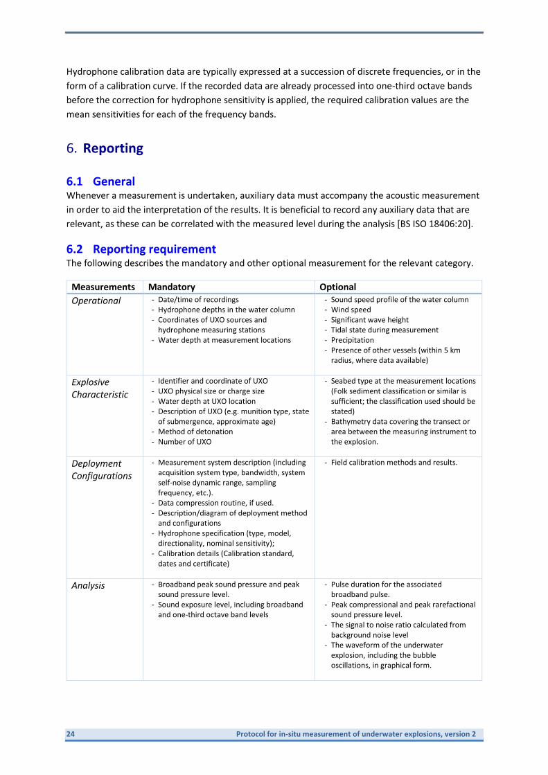
6.2 Reporting requirement The following describes the mandatory and other optional measurement for the relevant category.

Measurements Mandatory Optional

Operational - Date/time of recordings - Hydrophone depths in the water column - Coordinates of UXO sources and

hydrophone measuring stations - Water depth at measurement locations

- Sound speed profile of the water column - Wind speed - Significant wave height - Tidal state during measurement - Precipitation - Presence of other vessels (within 5 km

radius, where data available)

Explosive Characteristic

- Identifier and coordinate of UXO - UXO physical size or charge size - Water depth at UXO location - Description of UXO (e.g. munition type, state

of submergence, approximate age) - Method of detonation - Number of UXO

- Seabed type at the measurement locations (Folk sediment classification or similar is sufficient; the classification used should be stated)

- Bathymetry data covering the transect or area between the measuring instrument to the explosion.

Deployment Configurations

- Measurement system description (including acquisition system type, bandwidth, system self-noise dynamic range, sampling frequency, etc.).

- Data compression routine, if used. - Description/diagram of deployment method

and configurations - Hydrophone specification (type, model,

directionality, nominal sensitivity); - Calibration details (Calibration standard,

dates and certificate)

- Field calibration methods and results.

Analysis - Broadband peak sound pressure and peak sound pressure level.

- Sound exposure level, including broadband and one-third octave band levels

- Pulse duration for the associated broadband pulse.

- Peak compressional and peak rarefactional sound pressure level.

- The signal to noise ratio calculated from background noise level

- The waveform of the underwater explosion, including the bubble oscillations, in graphical form.


7. References

1. [Aarons, 1954] A. B. Aarons, “Underwater explosion shock wave parameters at large

distances from the charge,” J. Acoust. Soc. Am. 26, 343–346 (1954)

2. [Aarons et al 1949] A. B. Aarons, Cotter, T.P., “Long range shock propagation in underwater

explosion phenomena II” U.S. Navy Dept. Bur. Ord. NAVORD Rep 478, 1949

3. [André et al 2011] André, M., van der Schaar, M., Zaugg, S., Houégnigan, L., Sánchez, A., and

Castell, J. V., "Listening to the deep: Live monitoring of ocean noise and cetacean acoustic

signals", Marine Pollution Bulletin, vol. 63, 2011, pp. 18-26.

4. [ANSI/ASA S1.20-2012], Procedures for Calibration of Underwater Electroacoustic

Transducers, American National Standard Institute, USA, 2012

5. [BIAS, 2016]. BIAS Standard for Noise Measurements, Background information and

Guidelines https://biasproject.files.wordpress.com/2016/04/bias_standards_v5_final.pdf

6. [BS EN ISO 18406:2017], Underwater Acoustics – Measurement of Radiated Underwater

Sound from Percussive Pile Driving, ISO (the International Organization for Standardization),

Switzerland, 2017.

7. [BS EN ISO 18405:2017], Underwater Acoustics – Terminology, ISO (the International

Organization for Standardization), Switzerland, 2017.

8. [BS EN ISO 80000-8:2020], Quantities and units - Part 8: Acoustics, ISO (the International

Organization for Standardization), Switzerland, 2017.

9. [BS EN IEC 60565-1:2020] Underwater acoustics – Hydrophones – Calibration of

hydrophones – Part 1: Procedures for free-field calibration of hydrophones, International

Electrotechnical Commission, Geneva, Switzerland.

10. [BS EN IEC 60565-2:2019] Underwater acoustics – Hydrophones – Calibration of

hydrophones –Part 2: Procedures for low frequency pressure calibration, International

Electrotechnical Commission, Geneva, Switzerland.

11. [BS EN IEC 60500:2017] Underwater acoustics – Hydrophones – Properties of hydrophones

in the frequency range 1 Hz to 500 kHz, International Electrotechnical Commission, Geneva,

Switzerland, 2017.

12. [BS EN IEC 61260-1:2014], Electroacoustics — Octave-band and fractional-octave-band

filters, International Electrotechnical Commission, Geneva, Switzerland, 2014, (BS EN 61260-

1:2014).

13. [Cheong et al 2020] Cheong, S-H., Wang L., Lepper, P. and Robinson, S. “Characterisation of

Acoustic Fields Generated by UXO Removal - Phase 2 (Offshore Energy SEA Sub-Contract

OESEA-19-107), NPL Report AC 19, June 2020.

https://biasproject.files.wordpress.com/2016/04/bias_standards_v5_final.pdf


14. [EU TSG Noise 2014], “Monitoring Guidance for Underwater Noise in European Seas, Part II:

Monitoring Guidance Specifications”, Dekeling, R.P.A., Tasker, M.L., Van der Graaf, A.J.,

Ainslie, M.A, Andersson, M.H., André, M., Borsani, J.F., Brensing, K., Castellote, M., Cronin,

D., Dalen, J., Folegot, T., Leaper, R., Pajala, J., Redman, P., Robinson, S.P., Sigray, P., Sutton,

G., Thomsen, F., Werner, S., Wittekind, D., Young, J.V. JRC Scientific and Policy Report EUR

26555 EN, Publications Office of the, European Union, Luxembourg, 2014, doi:

10.2788/27158, ISBN 978-92-79-36339-9.

15. [Hayman et al 2017] "Calibration of marine autonomous acoustic recorders," Hayman G.,

Robinson S. P., Pangerc T., Ablitt J. Theobald P. D. OCEANS 2017 - Aberdeen, 2017, pp. 1-8.

DOI: 10.1109/OCEANSE.2017.8084773

16. [NPL, 2014]. Good Practice for Underwater Noise Measurement, National Measurement

Office, Marine Scotland, The Crown Estate, Robinson, S.P., Lepper, P. A. and Hazelwood,

R.A., NPL Good Practice Guide No. 133, ISSN: 1368-6550, 2014.

17. [JNCC 2010] JNCC guidelines for minimising the risk of injury to marine mammals from using

explosives, August 2010

18. [NMFS 2018] Technical Guidance for Assessing the Effects of Anthropogenic Sound on

Marine Mammal Hearing, US Dept. of Commer., NOAA. NOAA Technical Memorandum

NMFS-OPR- 59, 167p

19. [Reid 1993] “The response of surface ships to underwater explosions.” Reid, W.D. Australia

DSTO Aeronautical and Maritime Research Laboratory.

20. [Robinson et al 2020] Robinson S.P, Wang L, Cheong S-H, Lepper P.A., Marubini F, Hartley J

P. “Underwater acoustic characterisation of unexploded ordnance disposal using

deflagration”, Marine Pollution Bulletin, September 2020

21. [Snay 1956] “Hydrodynamics of underwater explosions”, Snay, H. Washington DC.:

Symposium on Naval Hydrodynamics, 1956

22. [Southall et al, 2019] “Marine Mammal Noise Exposure Criteria: Updated Scientific

Recommendations for Residual Hearing Effects”, Southall B.L., Finneran, J.J., Reichmuth, C.,

Nachtigall, P.E., Ketten, D.R., Bowles, A.E., Ellison, W.T., Nowacek, D.P., and Tyack, P.L.,

Aquatic Mammals 2019, 45(2), 125-232. DOI 10.1578/AM.45.2.2019.125

23. [Urick 1983] “Principles of underwater sound”, Urick, R.J. McGraw-Hill, New York, p. 423,

1983

[Weston 1960] “Underwater Explosions as Acoustic Sources”, Weston, D. E. Proceedings of

Physical Society vol 76(2) p233.249, 1960


Appendix A: Modelling of high order detonation

When explosive undergoes high order detonation, it creates a shock wave which the pressure can be approximated with exponential decay over time

𝑝(𝑡) = 𝑝𝑝𝑘𝑒−𝑡𝑡0

Where p(t) is the instantaneous pressure at time t after the beginning of the shock wave, ppk is the peak pressure at time = 0, and t0 is the exponential time constant. [Urick 1983] summarizes Aarons’ [Aarons et al 1949] semi-empirical work and provided a power law relationship between the peak pressure (µPa), charge weight (W) in kg and range (R), such that

𝑝𝑝𝑘 = 𝑘 (𝑊

13

𝑅)

𝛼

Where k and α are determined empirically. Based on this work, [Reid 1996] further developed the mathematical formulation based on different coefficients which depend on the type of explosive. It was observed that explosive type has a big influence on the peak pressure.

𝑝(𝑡) = 𝐾1 (𝑊

13

𝑅)

𝐴1

𝑒−

𝑡𝑡0

Similarly the time constant in microseconds, can be expressed in respect to charge weight of TNT and range.

𝑡0 = 𝐾2𝑊13 (

𝑊13

𝑅)

𝐴2

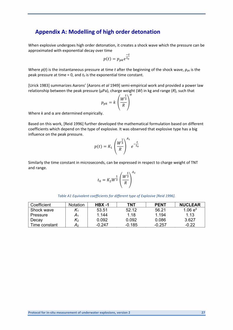
Table A1 Equivalent coefficients for different type of Explosive [Reid 1996].

Coefficient Notation HBX -1 TNT PENT NUCLEAR

Shock wave K1 53.51 52.12 56.21 1.06 e4

Pressure A1 1.144 1.18 1.194 1.13 Decay K2 0.092 0.092 0.086 3.627 Time constant A2 -0.247 -0.185 -0.257 -0.22


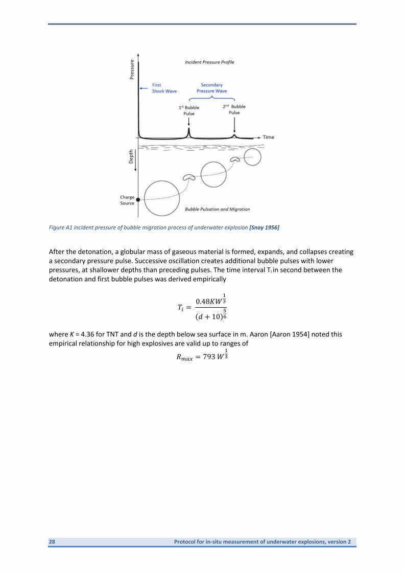
Figure A1 incident pressure of bubble migration process of underwater explosion [Snay 1956]

After the detonation, a globular mass of gaseous material is formed, expands, and collapses creating a secondary pressure pulse. Successive oscillation creates additional bubble pulses with lower pressures, at shallower depths than preceding pulses. The time interval Ti in second between the detonation and first bubble pulses was derived empirically

𝑇𝑖 = 0.48𝐾𝑊

13

(𝑑 + 10)56

where K = 4.36 for TNT and d is the depth below sea surface in m. Aaron [Aaron 1954] noted this empirical relationship for high explosives are valid up to ranges of

𝑅𝑚𝑎𝑥 = 793 𝑊13


Appendix B: Peak pressure signal processing considerations

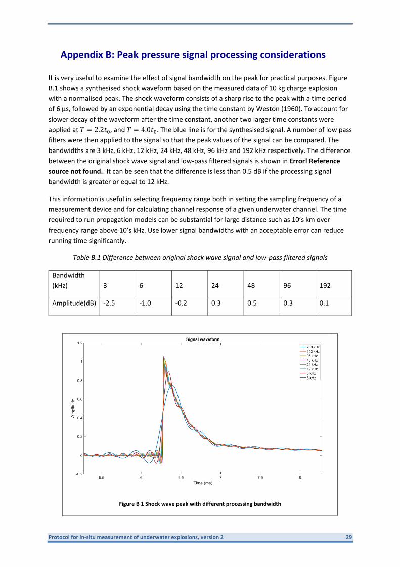
It is very useful to examine the effect of signal bandwidth on the peak for practical purposes. Figure

B.1 shows a synthesised shock waveform based on the measured data of 10 kg charge explosion

with a normalised peak. The shock waveform consists of a sharp rise to the peak with a time period

of 6 µs, followed by an exponential decay using the time constant by Weston (1960). To account for

slower decay of the waveform after the time constant, another two larger time constants were

applied at 𝑇 = 2.2𝑡0, and 𝑇 = 4.0𝑡0. The blue line is for the synthesised signal. A number of low pass

filters were then applied to the signal so that the peak values of the signal can be compared. The

bandwidths are 3 kHz, 6 kHz, 12 kHz, 24 kHz, 48 kHz, 96 kHz and 192 kHz respectively. The difference

between the original shock wave signal and low-pass filtered signals is shown in Error! Reference

source not found.. It can be seen that the difference is less than 0.5 dB if the processing signal

bandwidth is greater or equal to 12 kHz.

This information is useful in selecting frequency range both in setting the sampling frequency of a

measurement device and for calculating channel response of a given underwater channel. The time

required to run propagation models can be substantial for large distance such as 10’s km over

frequency range above 10’s kHz. Use lower signal bandwidths with an acceptable error can reduce

running time significantly.

Table B.1 Difference between original shock wave signal and low-pass filtered signals

Bandwidth

(kHz) 3 6 12 24 48 96 192

Amplitude(dB) -2.5 -1.0 -0.2 0.3 0.5 0.3 0.1

Figure B 1 Shock wave peak with different processing bandwidth


Documents

Protocol for in-situ measurement of underwater ... - GOV.UK