Protocol for estimating changes in the relative abundance of

deer in New Zealand forests using the Faecal Pellet Index (FPI)

David M. Forsyth Arthur Rylah Institute for Environmental Research 123 Brown Street, Heidelberg Victoria 3084, Australia Landcare Research Contract Report: LC0506/027 PREPARED FOR: Chief Scientist Department of Conservation P.O. Box 10-420 Wellington DATE: October 2005

Reviewed by: Bruce Warburton Scientist Landcare Research

Approved for release by: Phil Cowan Science Manager Biosecurity and Pest Management

© Department of Conservation 2005 This report has been produced by Landcare Research New Zealand Ltd for the New Zealand Department of Conservation. All copyright in this report is the property of the Crown and any unauthorised publication, reproduction, or adaptation of this report is a breach of that copyright and illegal.

Landcare Research

3

Contents

1. Introduction .......................................................................................................................5 2. Intended Use of this Protocol ............................................................................................5 3. Faecal Pellet Index (FPI) Protocol ....................................................................................6

3.1 Designing the monitoring programme .....................................................................6 3.1.1 Define the study area .................................................................................6 3.1.2 Exclude areas that cannot be sampled .......................................................6 3.1.3 Stratification of the study area ...................................................................6 3.1.4 Number of transects ...................................................................................6 3.1.5 Transect start points and bearings..............................................................6

3.2 Repeated sampling of study areas............................................................................7 3.3 Field monitoring.......................................................................................................8

3.3.1 Transects ....................................................................................................8 3.3.2 Running-line ..............................................................................................8 3.3.3 Counting pellets and pellet groups.............................................................8 3.3.4 Recording pellets and pellet groups.........................................................10

3.4 Entering and storing data .......................................................................................11 3.5 Analyses .................................................................................................................11

3.5.1 Summarising data from one survey .........................................................11 3.5.2 Estimating the change in deer density following a second survey ..........18

4. Using the same observers in repeat surveys ....................................................................21 5. How long will sampling take?.........................................................................................21 6. Training ...........................................................................................................................21 7. Acknowledgements .........................................................................................................22 8. References .......................................................................................................................22

Appendix 1 Definition of intact pellets ........................................................................23 Appendix 2. Spreadsheet used to store FPI data............................................................24

4

Landcare Research

Landcare Research

5

1. Introduction This protocol was developed for Department of Conservation staff, and contractors employed by the Department, to use to estimate changes in the abundance of deer in forests. The protocol is based on counts of faecal pellets along randomly located transects. Many elements of the design of this protocol are shared with the National Trap-Catch Protocol (National Possum Control Agencies 2004): this was intentional because many staff and contractors likely to use this protocol will be familiar with the National Trap-Catch Protocol. 2. Intended Use of this Protocol This protocol provides a method of estimating long-term changes in the relative abundance of deer in New Zealand forests. The relationship between the index calculated following this protocol (termed the Faecal Pellet Index, or ‘FPI’) and the density of deer has been estimated using 20 enclosures with known densities of deer (12 in the South Island and 8 in the North Island). For the range of deer densities in the 20 enclosures, the relationship was approximately linear. Given that linear relationship, the calculations for estimating the change in deer density from the index are straightforward (see below; D. M. Forsyth et al. unpublished manuscript1). Previous protocols (Bell 1973; Baddeley 1985; Fraser 1998) have suggested that the number of deer living in a forest can be estimated if three variables are known: (i) the amount or ‘standing crop’ of faecal pellets; (ii) the rate at which those faecal pellets were deposited by the deer; and (iii) the rate at which those faecal pellets have decayed. It is difficult and expensive to estimate the rate at which wild deer deposit faecal pellets in a forest, so previous studies have assumed a rate based on overseas work. There is also debate about the accuracy of estimates of the standing crop and about the best way to estimate decay rates. Estimates of the number of deer in a forest using faecal pellets will be prohibitively expensive if all three variables are estimated at that site, or are likely to be inaccurate if non site-specific estimates of pellet deposition and decay are used. Hence, attempting to estimate the number of deer in an area of forest is not recommended. We also emphasise that the figures in D. M. Forsyth et al. (unpublished manuscript) should not be inverted to provide estimates of deer density from FPI data because of the presence of covariate effects in those relationships. The standing crop of pellets estimated with this protocol should not be compared to estimates from previous protocols (Bell 1973; Baddeley 1985) for two main reasons. First, previous estimates were based on semi-random sampling. In particular, transects started at water-courses and ended at ridge tops (Baddeley 1985). Random sampling means that each point in the study area has the same probability of being sampled; this is not the case for semi-random sampling. Random sampling is necessary if inferences about changes in deer density are to apply to all of the study area. Second, the two methods differ in the number of intact pellets included in a ‘group’ and on the need to search outside the plot to determine whether pellets are counted or not. The FPI described here is not attempting to estimate the standing crop so that absolute deer density (number/km2) can be estimated (e.g., by using estimates of faecal deposition and decay rates, as has been done previously; Baddeley 1985): rather, it is a standardised method that produces a pellet count that has a positive and approximately linear relationship with deer density for the range of densities used in the calibration. Unlike the National Trap-Catch Protocol, this protocol should not be used to estimate the kill rate of deer achieved by control operations. Because faecal pellets may take many months to decay, the FPI is unsuitable for estimating kill rates. The best way to estimate kill rates in a control operation is to use mortality-sensing radio-collars on a random sample of animals (see Warburton et al. 2004 for the

1 The unpublished manuscript is available from the author (E-mail: dave.forsyth@dse.vic.gov.au).

6

Landcare Research

application of this technique to the estimation of possum kill rates). Capturing and placing collars on a reasonable sample of deer (i.e., >20) in a forest will be expensive (Nugent and Yockney 2004). 3. Faecal Pellet Index (FPI) Protocol 3.1 Designing the monitoring programme 3.1.1 Define the study area Draw on a map (no less detailed than 1:50,000) the boundary of the area that you are interested in. 3.1.2 Exclude areas that cannot be sampled Draw on the map the boundaries of any areas that cannot be sampled due to rugged terrain (e.g., bluffs) or the presence of waterbodies (i.e., lakes, tarns and large rivers). 3.1.3 Stratification of the study area If you expect deer densities to vary over the study area, then the study area should be sub-divided. Examples might be substantial areas of grassland and forest (which deer might use differently and in which deer may differ in their vulnerability to hunting), or areas subject to either helicopter-based or ground-based hunting. The boundaries of these ‘strata’ are drawn on the map, and changes in deer density are estimated separately for each ‘stratum’. In other words, each stratum is considered a separate study area. 3.1.4 Number of transects There must be a minimum of 30 transects per study area (or stratum). The eight study areas in the Department’s Deer Forest Study (Investigation Number 3673) will each have 50 transects (C. Veltman, Department of Conservation, personal communication). 3.1.5 Transect start points and bearings For reasons outlined above in Section 2, it is desirable that each point in the study area has the same probability of being sampled. Hence, transect start points and bearings are determined using random numbers. Some GIS packages can provide randomly located start points. For people without access to such a GIS, random start points (Eastings and Northings) can be assigned using either a table of random numbers (e.g., Table 10 in Rohlf and Sokal 1981) or a random number generator. Map squares in the NZMS 260 map series (1:50,000) are 1×1 km, and it is suggested that start points are assigned at the 1 m scale: this has the advantage that the coordinates can be downloaded into a hand-held GPS. For readers familiar with Microsoft® Excel, random numbers can be generated using the random number generator function as follows: Eastings are generated using the equation: =RANDBETWEEN(x1, x2) where x1 and x2 are the western- and eastern-most map coordinates, respectively, of the study area (e.g., 2730000 and 2736000 for the Waihaha study area; see below). Northings are generated using the equation: =RANDBETWEEN(y1, y2)

Landcare Research

7

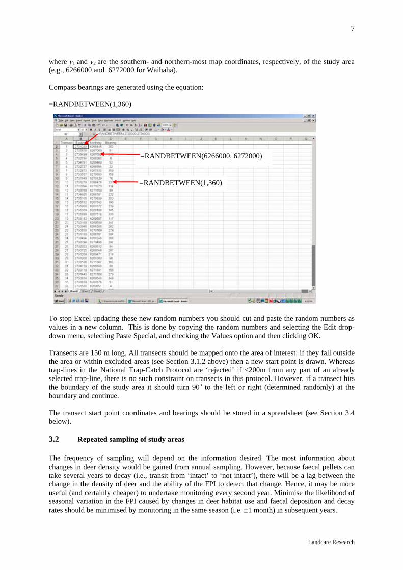
where y1 and y2 are the southern- and northern-most map coordinates, respectively, of the study area (e.g., 6266000 and 6272000 for Waihaha). Compass bearings are generated using the equation: =RANDBETWEEN(1,360) To stop Excel updating these new random numbers you should cut and paste the random numbers as values in a new column. This is done by copying the random numbers and selecting the Edit drop-down menu, selecting Paste Special, and checking the Values option and then clicking OK. Transects are 150 m long. All transects should be mapped onto the area of interest: if they fall outside the area or within excluded areas (see Section 3.1.2 above) then a new start point is drawn. Whereas trap-lines in the National Trap-Catch Protocol are ‘rejected’ if <200m from any part of an already selected trap-line, there is no such constraint on transects in this protocol. However, if a transect hits the boundary of the study area it should turn 90o to the left or right (determined randomly) at the boundary and continue. The transect start point coordinates and bearings should be stored in a spreadsheet (see Section 3.4 below). 3.2 Repeated sampling of study areas The frequency of sampling will depend on the information desired. The most information about changes in deer density would be gained from annual sampling. However, because faecal pellets can take several years to decay (i.e., transit from ‘intact’ to ‘not intact’), there will be a lag between the change in the density of deer and the ability of the FPI to detect that change. Hence, it may be more useful (and certainly cheaper) to undertake monitoring every second year. Minimise the likelihood of seasonal variation in the FPI caused by changes in deer habitat use and faecal deposition and decay rates should be minimised by monitoring in the same season (i.e. ±1 month) in subsequent years.

=RANDBETWEEN(6266000, 6272000)

=RANDBETWEEN(1,360)

8

Landcare Research

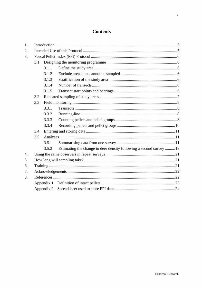
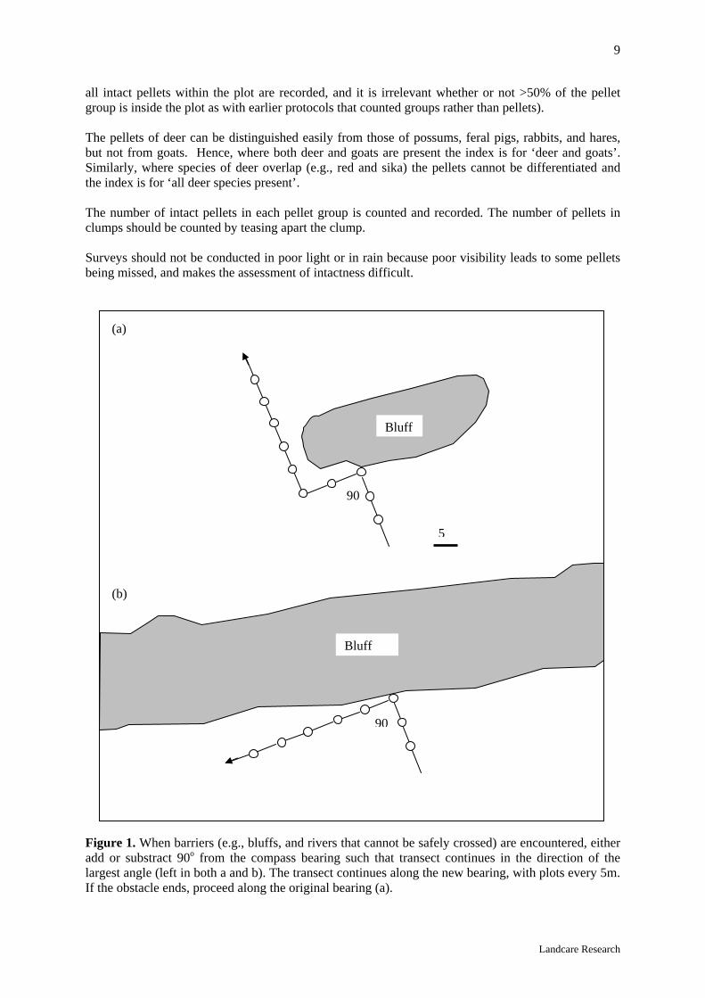
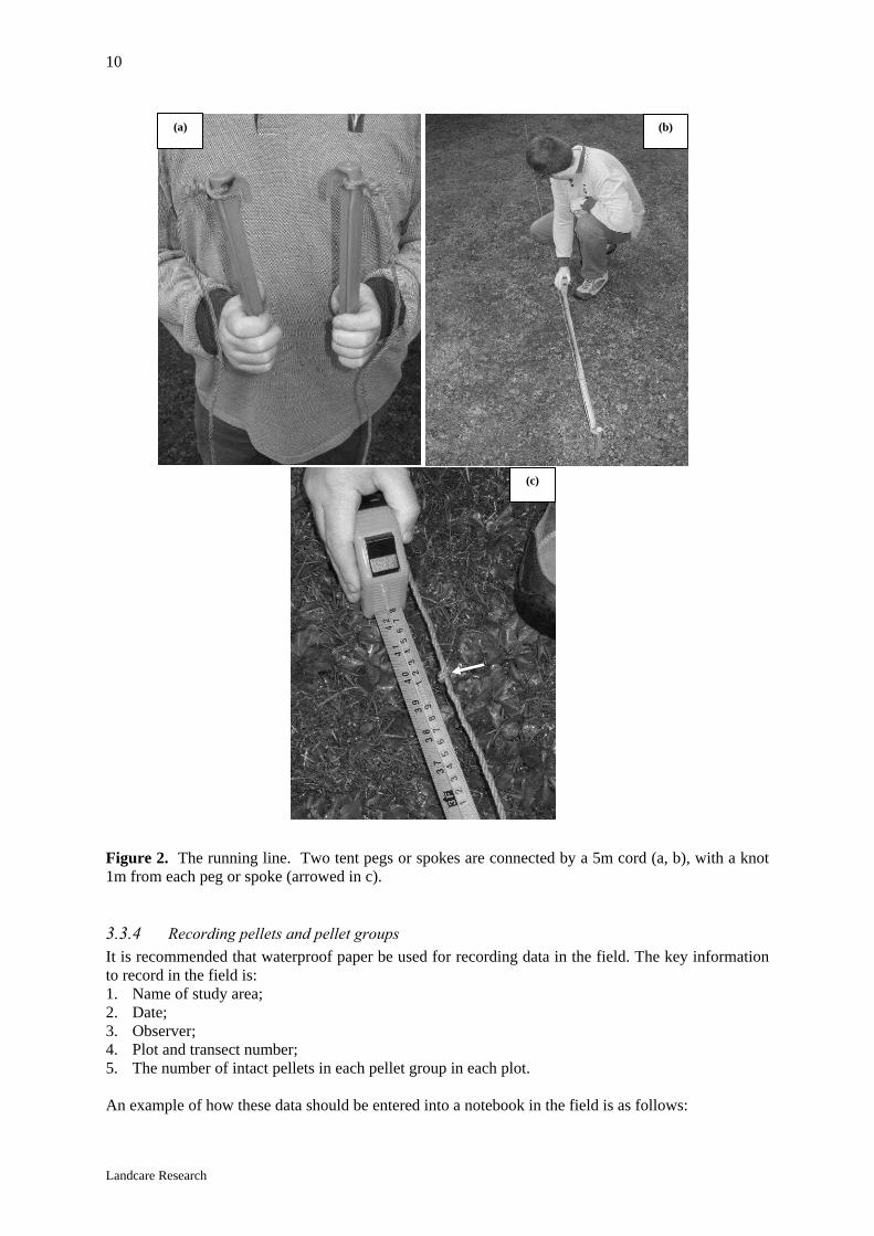
Transects are not permanently marked because there is data suggesting that deer defecate less in marked plots (Nugent et al. 1997). However, the same transect start-points and bearings are used in subsequent monitoring in the study area. If possible, the same observers should monitor the same transects over time. 3.3 Field monitoring 3.3.1 Transects Navigate to the start point of the transect using a combination of GPS, map, compass, and hip-chain. It is critical that the transect starts on the stipulated start-point and follows the designated bearing. If the start point cannot safely be reached then that start point must be discarded and that area excluded from subsequent sampling (see section 3.1.2 above): a new start point must be generated by the survey designer (i.e., randomly). Place one of the running-line’s pegs (see Section 3.3.2 below) into the ground. Set your compass to the required bearing and move in that direction. When the running-line is taut, place the second peg into the ground and gently pull on the string so that the other peg pulls out of the ground. A knot on the running line is then used to delineate a circular plot (of 1-m radius) in which intact faecal pellets are counted (see Section 3.3.3 below). When the plot has been thoroughly searched continue on the compass bearing for 5m until the running line is taut and insert the peg: this is the next plot. This procedure is repeated on the same compass bearing until 30 plots have been completed (i.e. each transect is 150 m). Note that the first plot is 5 m from the transect start point, not at the start point. When barriers (e.g., bluffs and rivers that cannot be safely crossed) are encountered, either add or substract 90o from the compass bearing such that the transect continues in the direction of the largest angle (see Figure 1). The transect continues along the new bearing, with plots every 5m. If the obstacle ends, proceed on the original bearing (Figure 1). This will, on occasions, bias the plots towards ‘edges’ and so perhaps towards favoured areas for deer, but practicality must rule over rigour in this case. 3.3.2 Running-line The running-line consists of two pegs (e.g., tent pegs or bicycle spokes, approximate length 15–25 cm) connected by a 5-m non-stretch cord (Figure 2a,b). On the 5-m cord there are two knots, each 1-m from either peg (Figure 2c): this knot defines the radius of the circular plot to be searched. The running line should be checked prior to starting the first transect on each day to ensure that the string between the pegs is 5-m long and that the plot markers are exactly 1m from the pegs. 3.3.3 Counting pellets and pellet groups Within each plot of 1-m radius, vegetation (including fern fronds/small branches) is pushed aside to ensure that the entire plot surface is searched, but the litter layer is not disturbed. The plot is searched systematically and the number of intact pellets is counted and recorded. An intact pellet is defined (following Baddeley 1985) as having no recognisable loss of material, regardless of whether the pellet is cracked, partly broken or deformed (e.g., by trampling). The presence of moss or fungus does not affect whether a pellet is considered intact or not. Photographs of pellets that are and are not intact are presented in Appendix 1, and it is recommended that a laminated colour copy of Appendix 1 is carried in the field for consultation. A pellet group is defined as ‘intact pellets voided in the same defecation’, and is determined by appearance (i.e., size, shape and colour). Note that, in contrast to previous work, (i) a pellet group may consist of one or more intact pellets (i.e., a single pellet is the minimum number of intact pellets required to constitute a pellet group within the plot, and (ii) no searching occurs outside the plot (i.e.,

Landcare Research

9

all intact pellets within the plot are recorded, and it is irrelevant whether or not >50% of the pellet group is inside the plot as with earlier protocols that counted groups rather than pellets). The pellets of deer can be distinguished easily from those of possums, feral pigs, rabbits, and hares, but not from goats. Hence, where both deer and goats are present the index is for ‘deer and goats’. Similarly, where species of deer overlap (e.g., red and sika) the pellets cannot be differentiated and the index is for ‘all deer species present’. The number of intact pellets in each pellet group is counted and recorded. The number of pellets in clumps should be counted by teasing apart the clump. Surveys should not be conducted in poor light or in rain because poor visibility leads to some pellets being missed, and makes the assessment of intactness difficult. Figure 1. When barriers (e.g., bluffs, and rivers that cannot be safely crossed) are encountered, either add or substract 90o from the compass bearing such that transect continues in the direction of the largest angle (left in both a and b). The transect continues along the new bearing, with plots every 5m. If the obstacle ends, proceed along the original bearing (a).

5

Bluff

Bluff

(b)

(a)

90

90

10

Landcare Research

Figure 2. The running line. Two tent pegs or spokes are connected by a 5m cord (a, b), with a knot 1m from each peg or spoke (arrowed in c). 3.3.4 Recording pellets and pellet groups It is recommended that waterproof paper be used for recording data in the field. The key information to record in the field is: 1. Name of study area; 2. Date; 3. Observer; 4. Plot and transect number; 5. The number of intact pellets in each pellet group in each plot. An example of how these data should be entered into a notebook in the field is as follows:

(a)

(c)

(b)

Landcare Research

11

Waihaha, 6 May 2005, Stephen Roberts Transect 11. 1 ∅, 2 ∅, 3 (9, 15), 4 ∅, 5 ∅, 6 (8, 15), 7 (31, 30), 8 ∅, 9 ∅, 10 ∅, 11 ∅, 12 (45), 13 ∅, 14 ∅, 15 ∅, 16 ∅, 17 (5, 4), 18 ∅, 19 ∅, 20 (49), 21 (18), 22 ∅, 23 ∅, 24 ∅, 25 ∅, 26 ∅, 27 ∅, 28 ∅, 29 ∅, 30 ∅. A zero count is indicated by a zero with a strike through it, plots (always 30 per transect) are separated by commas and intact pellets are recorded as the number within each pellet group in parentheses. In the above example, no intact pellets were recorded on plots 1 and 2, but on plot 3 there were two pellet groups (one with 9 intact pellets and one with 15 intact pellets). A pellet group may contain 1 or hundreds of intact pellets. 3.4 Entering and storing data The field data should be entered into a spreadsheet as soon as possible by the person who collected the data, and checked for errors. The field data (and maps defining the study area) should then be stored on file for future consultation. The spreadsheet shown in Appendix 2 should be used to store the field data. It is important that both the first name (or initial) and surname of the person(s) who collected the data are entered in the ‘Observer’ column: if one person counted the pellets and the other recorded (the recommended practice for two people working together) then the name of the person counting the pellets should be recorded. (Note that for transect 12 in Appendix 2 both observers counted pellets.) Column A (‘Study area’) is the name of the study area. Columns B–D (‘Easting’, ‘Northing’ and ‘Bearing’) refer to the start points and coordinates for each transect (not each plot!). Column E (‘Date’) is the date when the transect was monitored, and Column F (‘Observer’) is the name of the person(s) who counted the pellets. Columns G and H (‘Transect’ and ‘Plot’) refer to the transect and plot numbers; there should always be 30 plots per transect. Column I (‘Pellets by group’) is the number of intact pellets in each of the pellet groups present in that plot. Field data must be entered in the style shown here, with zeros denoted by zero (NOT a dash or empty cell) and pellet group sizes separated by commas and a space. Column J (‘Total pellets’) is the sum of the pellet group sizes in column I. A real example of recording data for a study area is provided in a worksheet (‘Data for one survey’ in the downloadable Excel file. 3.5 Analyses Information from two surveys is needed to estimate a change in deer density. However, after the first survey these steps can be followed to calculate the Faecal Pellet Index (FPI) for the study area: 3.5.1 Summarising data from one survey A mean and 95% confidence interval (CI) for the FPI can be calculated for the first survey as follows. Note that these data and outputs can be accessed in the spreadsheets ‘Data for one survey’ and ‘Statistics for one survey’ in the downloadable Excel file.

12

Landcare Research

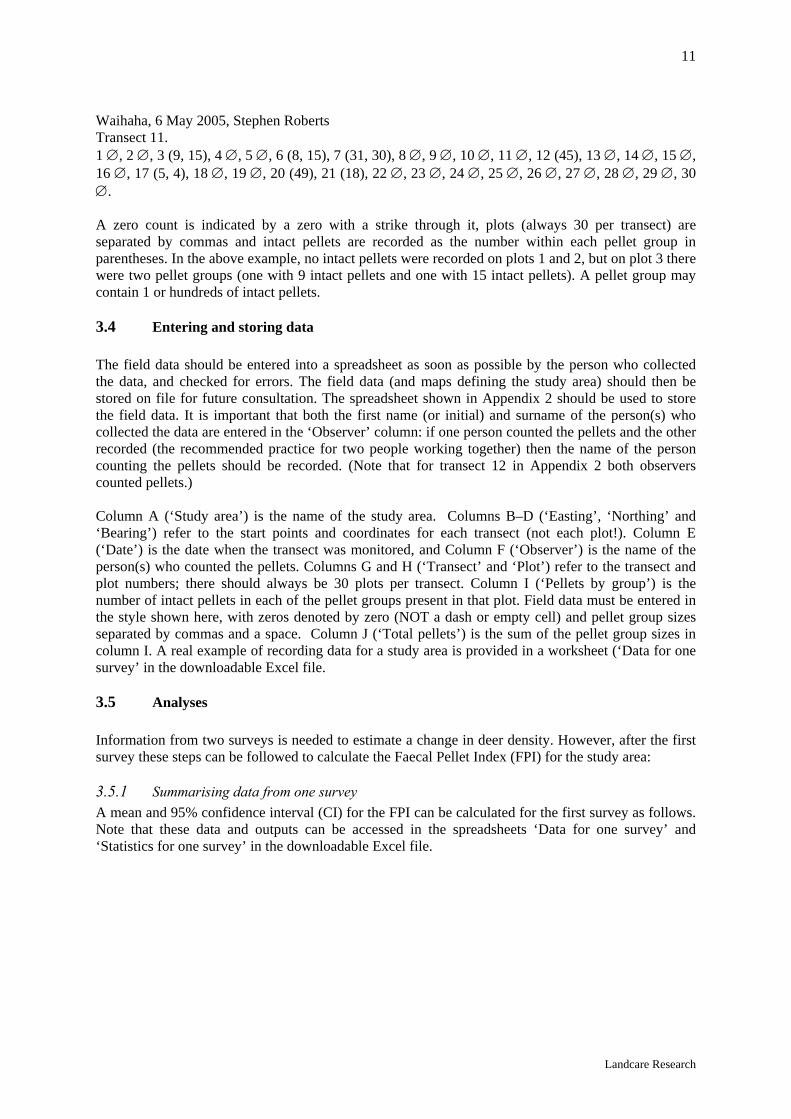
1. Calculate the total number of intact faecal pellets for each transect. These transect totals should be stored in a separate column, and can be calculated quickly in Excel using the Pivot Table function as follows. First, select the ‘Data’ tab and click on ‘Pivot Table Report’.

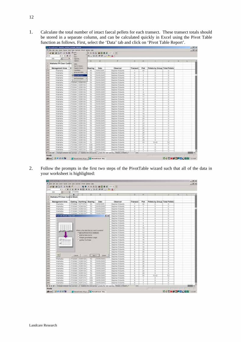
2. Follow the prompts in the first two steps of the PivotTable wizard such that all of the data in

your worksheet is highlighted:

Landcare Research

13

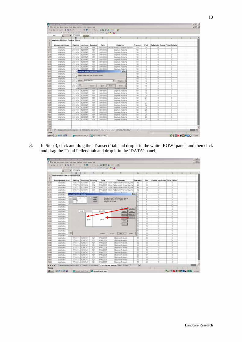
3. In Step 3, click and drag the ‘Transect’ tab and drop it in the white ‘ROW’ panel, and then click

and drag the ‘Total Pellets’ tab and drop it in the ‘DATA’ panel;

14

Landcare Research

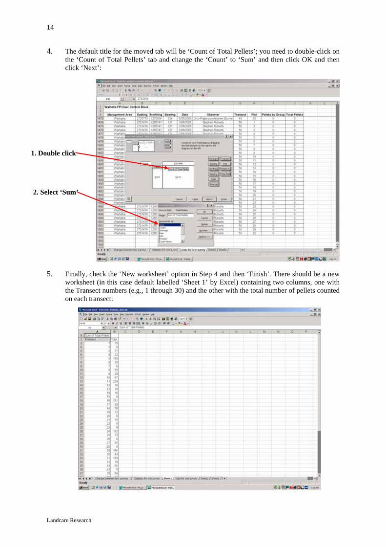
4. The default title for the moved tab will be ‘Count of Total Pellets’; you need to double-click on the ‘Count of Total Pellets’ tab and change the ‘Count’ to ‘Sum’ and then click OK and then click ‘Next’:

5. Finally, check the ‘New worksheet’ option in Step 4 and then ‘Finish’. There should be a new

worksheet (in this case default labelled ‘Sheet 1’ by Excel) containing two columns, one with the Transect numbers (e.g., 1 through 30) and the other with the total number of pellets counted on each transect:

1. Double click

2. Select ‘Sum’

Landcare Research

15

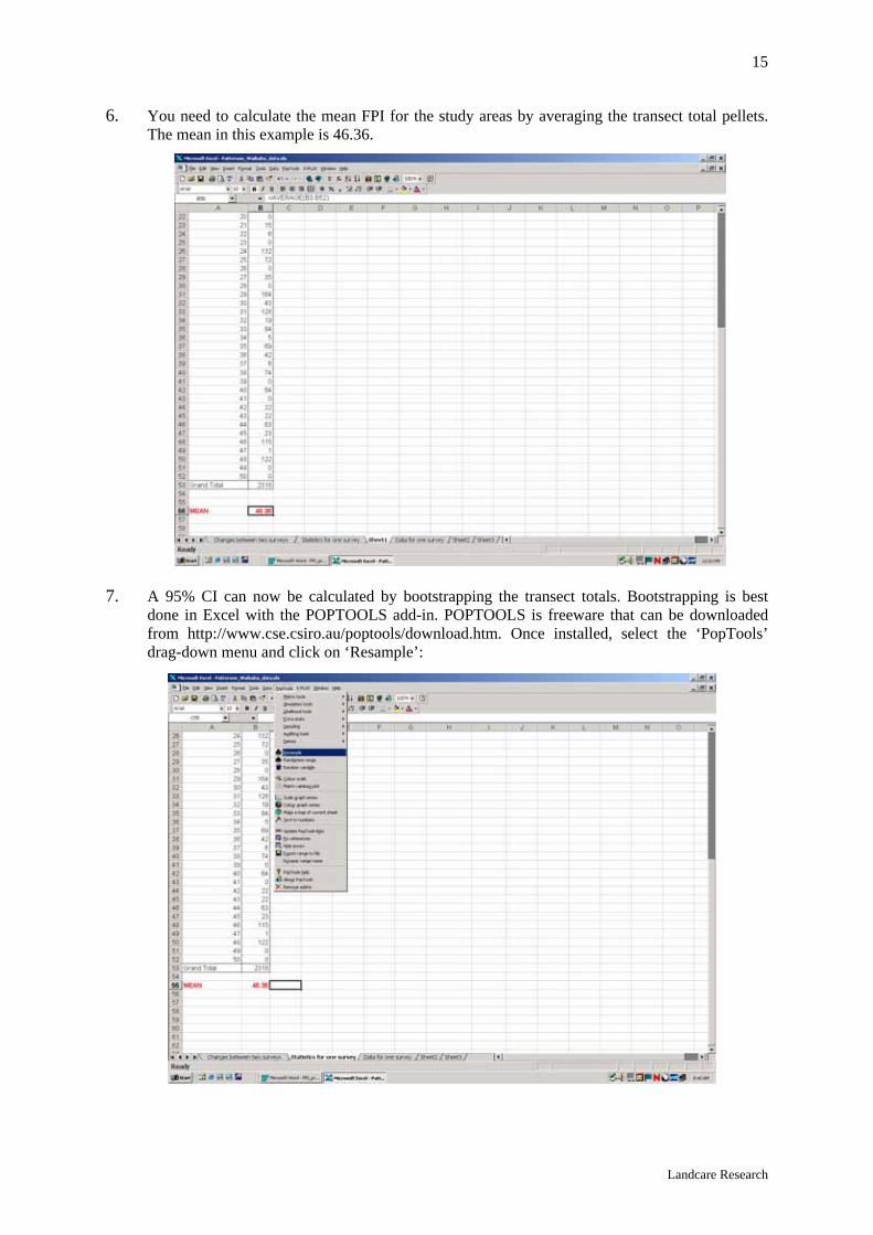
6. You need to calculate the mean FPI for the study areas by averaging the transect total pellets. The mean in this example is 46.36.

7. A 95% CI can now be calculated by bootstrapping the transect totals. Bootstrapping is best

done in Excel with the POPTOOLS add-in. POPTOOLS is freeware that can be downloaded from http://www.cse.csiro.au/poptools/download.htm. Once installed, select the ‘PopTools’ drag-down menu and click on ‘Resample’:

16

Landcare Research

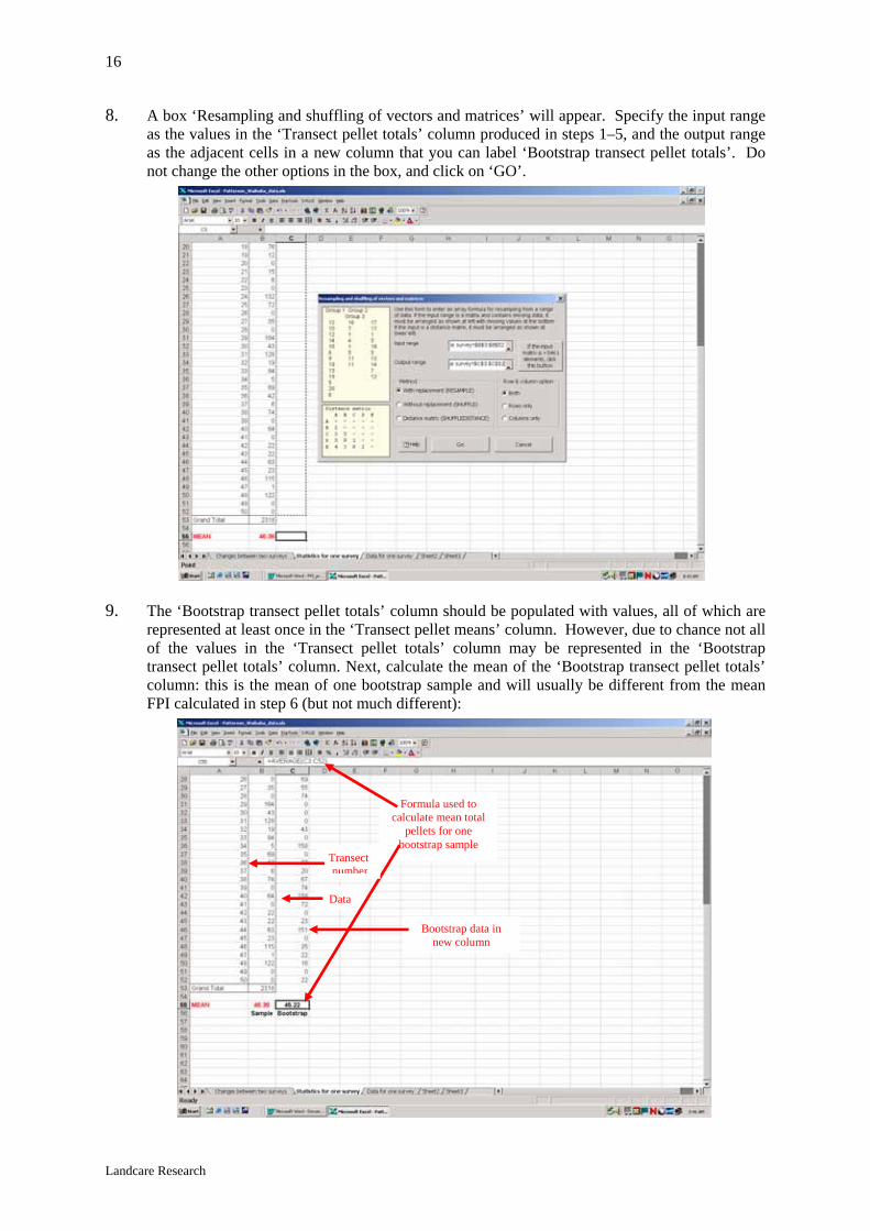
8. A box ‘Resampling and shuffling of vectors and matrices’ will appear. Specify the input range as the values in the ‘Transect pellet totals’ column produced in steps 1–5, and the output range as the adjacent cells in a new column that you can label ‘Bootstrap transect pellet totals’. Do not change the other options in the box, and click on ‘GO’.

9. The ‘Bootstrap transect pellet totals’ column should be populated with values, all of which are

represented at least once in the ‘Transect pellet means’ column. However, due to chance not all of the values in the ‘Transect pellet totals’ column may be represented in the ‘Bootstrap transect pellet totals’ column. Next, calculate the mean of the ‘Bootstrap transect pellet totals’ column: this is the mean of one bootstrap sample and will usually be different from the mean FPI calculated in step 6 (but not much different):

Formula used to calculate mean total

pellets for one bootstrap sample

Bootstrap data in new column

Data

Transectnumber

Landcare Research

17

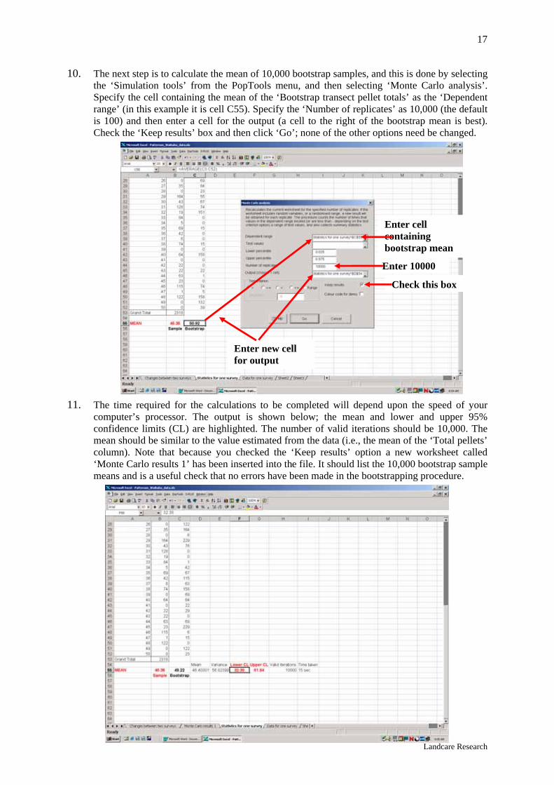
10. The next step is to calculate the mean of 10,000 bootstrap samples, and this is done by selecting the ‘Simulation tools’ from the PopTools menu, and then selecting ‘Monte Carlo analysis’. Specify the cell containing the mean of the ‘Bootstrap transect pellet totals’ as the ‘Dependent range’ (in this example it is cell C55). Specify the ‘Number of replicates’ as 10,000 (the default is 100) and then enter a cell for the output (a cell to the right of the bootstrap mean is best). Check the ‘Keep results’ box and then click ‘Go’; none of the other options need be changed.

11. The time required for the calculations to be completed will depend upon the speed of your

computer’s processor. The output is shown below; the mean and lower and upper 95% confidence limits (CL) are highlighted. The number of valid iterations should be 10,000. The mean should be similar to the value estimated from the data (i.e., the mean of the ‘Total pellets’ column). Note that because you checked the ‘Keep results’ option a new worksheet called ‘Monte Carlo results 1’ has been inserted into the file. It should list the 10,000 bootstrap sample means and is a useful check that no errors have been made in the bootstrapping procedure.

Enter cell containing bootstrap mean

Check this box

Enter 10000

Enter new cell for output

18

Landcare Research

12. The mean FPI (from the sample data rather than the bootstrap mean) and 95% CI are the statistics of interest, and are highlighted in the example above: the mean FPI is 46.4 and the 95% CI is 32.4–61.9.

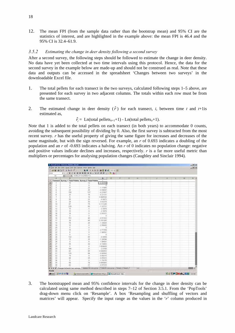
3.5.2 Estimating the change in deer density following a second survey After a second survey, the following steps should be followed to estimate the change in deer density. No data have yet been collected at two time intervals using this protocol. Hence, the data for the second survey in the example below are made-up and should not be construed as real. Note that these data and outputs can be accessed in the spreadsheet ‘Changes between two surveys’ in the downloadable Excel file. 1. The total pellets for each transect in the two surveys, calculated following steps 1–5 above, are

presented for each survey in two adjacent columns. The totals within each row must be from the same transect.

2. The estimated change in deer density ( r̂ ) for each transect, i, between time t and t+1is

estimated as, ir̂ = Ln(total pelletsit+1+1) - Ln(total pelletsit+1).

Note that 1 is added to the total pellets on each transect (in both years) to accommodate 0 counts, avoiding the subsequent possibility of dividing by 0. Also, the first survey is subtracted from the most recent survey. r has the useful property of giving the same figure for increases and decreases of the same magnitude, but with the sign reversed. For example, an r of 0.693 indicates a doubling of the population and an r of -0.693 indicates a halving. An r of 0 indicates no population change: negative and positive values indicate declines and increases, respectively. r is a far more useful metric than multipliers or percentages for analysing population changes (Caughley and Sinclair 1994).

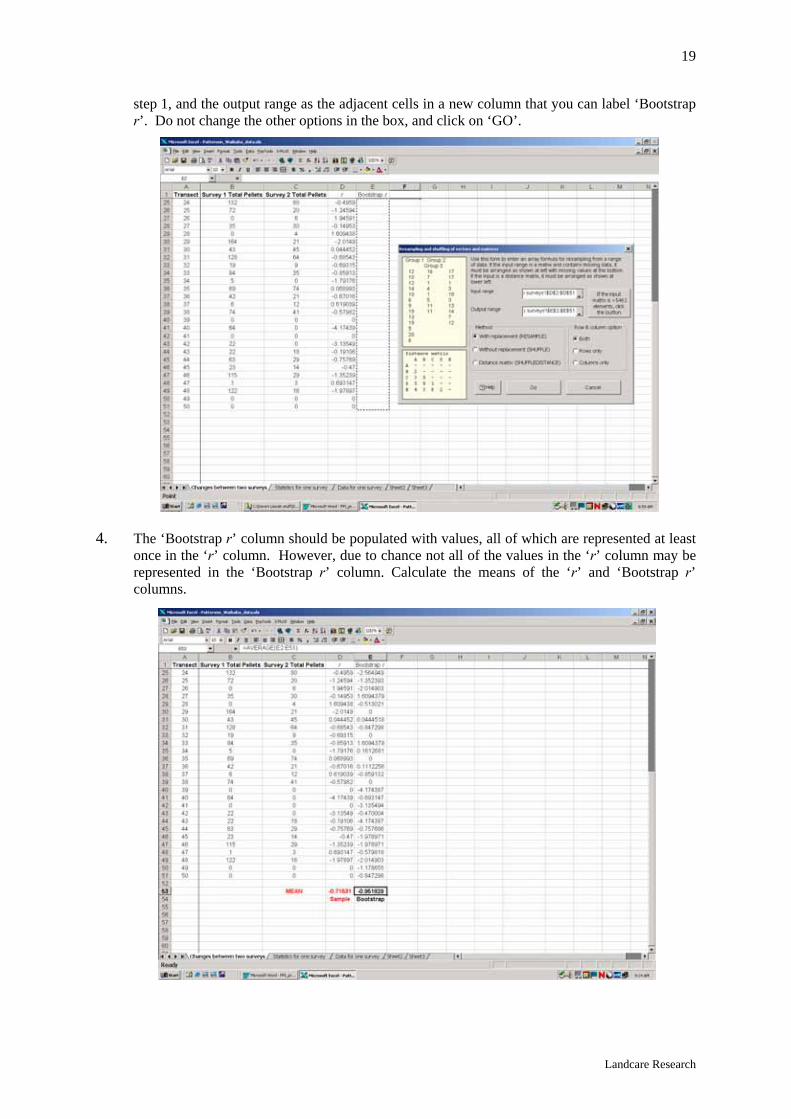
3. The bootstrapped mean and 95% confidence intervals for the change in deer density can be

calculated using same method described in steps 7–12 of Section 3.5.1. From the ‘PopTools’ drag-down menu click on ‘Resample’. A box ‘Resampling and shuffling of vectors and matrices’ will appear. Specify the input range as the values in the ‘r’ column produced in

Landcare Research

19

step 1, and the output range as the adjacent cells in a new column that you can label ‘Bootstrap r’. Do not change the other options in the box, and click on ‘GO’.

4. The ‘Bootstrap r’ column should be populated with values, all of which are represented at least

once in the ‘r’ column. However, due to chance not all of the values in the ‘r’ column may be represented in the ‘Bootstrap r’ column. Calculate the means of the ‘r’ and ‘Bootstrap r’ columns.

20

Landcare Research

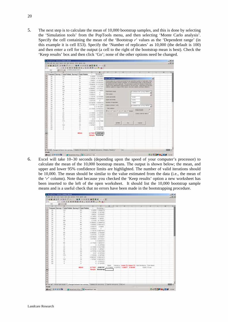
5. The next step is to calculate the mean of 10,000 bootstrap samples, and this is done by selecting the ‘Simulation tools’ from the PopTools menu, and then selecting ‘Monte Carlo analysis’. Specify the cell containing the mean of the ‘Bootstrap r’ values as the ‘Dependent range’ (in this example it is cell E53). Specify the ‘Number of replicates’ as 10,000 (the default is 100) and then enter a cell for the output (a cell to the right of the bootstrap mean is best). Check the ‘Keep results’ box and then click ‘Go’; none of the other options need be changed.

6. Excel will take 10–30 seconds (depending upon the speed of your computer’s processor) to calculate the mean of the 10,000 bootstrap means. The output is shown below; the mean, and upper and lower 95% confidence limits are highlighted. The number of valid iterations should be 10,000. The mean should be similar to the value estimated from the data (i.e., the mean of the ‘r’ column). Note that because you checked the ‘Keep results’ option a new worksheet has been inserted to the left of the open worksheet. It should list the 10,000 bootstrap sample means and is a useful check that no errors have been made in the bootstrapping procedure.

Landcare Research

21

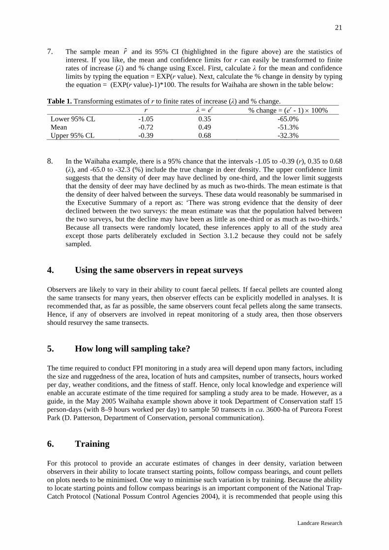
7. The sample mean r̂ and its 95% CI (highlighted in the figure above) are the statistics of interest. If you like, the mean and confidence limits for r can easily be transformed to finite rates of increase (λ) and % change using Excel. First, calculate λ for the mean and confidence limits by typing the equation = EXP(r value). Next, calculate the % change in density by typing the equation = (EXP(r value)-1)*100. The results for Waihaha are shown in the table below:

Table 1. Transforming estimates of r to finite rates of increase (λ) and % change. r λ = er % change = (er - 1) × 100% Lower 95% CL -1.05 0.35 -65.0% Mean -0.72 0.49 -51.3% Upper 95% CL -0.39 0.68 -32.3%

8. In the Waihaha example, there is a 95% chance that the intervals -1.05 to -0.39 (r), 0.35 to 0.68

(λ), and -65.0 to -32.3 (%) include the true change in deer density. The upper confidence limit suggests that the density of deer may have declined by one-third, and the lower limit suggests that the density of deer may have declined by as much as two-thirds. The mean estimate is that the density of deer halved between the surveys. These data would reasonably be summarised in the Executive Summary of a report as: ‘There was strong evidence that the density of deer declined between the two surveys: the mean estimate was that the population halved between the two surveys, but the decline may have been as little as one-third or as much as two-thirds.’ Because all transects were randomly located, these inferences apply to all of the study area except those parts deliberately excluded in Section 3.1.2 because they could not be safely sampled.

4. Using the same observers in repeat surveys Observers are likely to vary in their ability to count faecal pellets. If faecal pellets are counted along the same transects for many years, then observer effects can be explicitly modelled in analyses. It is recommended that, as far as possible, the same observers count fecal pellets along the same transects. Hence, if any of observers are involved in repeat monitoring of a study area, then those observers should resurvey the same transects. 5. How long will sampling take? The time required to conduct FPI monitoring in a study area will depend upon many factors, including the size and ruggedness of the area, location of huts and campsites, number of transects, hours worked per day, weather conditions, and the fitness of staff. Hence, only local knowledge and experience will enable an accurate estimate of the time required for sampling a study area to be made. However, as a guide, in the May 2005 Waihaha example shown above it took Department of Conservation staff 15 person-days (with 8–9 hours worked per day) to sample 50 transects in ca. 3600-ha of Pureora Forest Park (D. Patterson, Department of Conservation, personal communication). 6. Training For this protocol to provide an accurate estimates of changes in deer density, variation between observers in their ability to locate transect starting points, follow compass bearings, and count pellets on plots needs to be minimised. One way to minimise such variation is by training. Because the ability to locate starting points and follow compass bearings is an important component of the National Trap-Catch Protocol (National Possum Control Agencies 2004), it is recommended that people using this

22

Landcare Research

protocol have completed the ‘Field Operative’ training course for the National Trap-Catch Protocol (contact National Possum Control Agencies, PO Box 11-461, Wellington; Tel: (04) 499 7559; E-mail: npca@xtra.co.nz). Training requirements for the use of this protocol by DOC staff and contractors are being finalised. However, in the interim it is recommended that staff using this protocol are trained by someone who has used the protocol, ideally working alongside someone in a survey before working alone. An obvious source of variation will be the definition of intact pellets. It is recommended that a laminated colour copy of Appendix 1 is carried in the field for consultation. 7. Acknowledgements This study was conducted under contract to the Department of Conservation (Investigation Number 3589). I thank Clare Veltman (Department of Conservation) for commissioning the work. Richard Barker (University of Otago) developed the statistical models underlying this protocol; those models are reported in an unpublished manuscript available from the author. Grant Morriss, Nick Poutu, Ben Reddiex (all Landcare Research), Ryan Chick (Arthur Rylah Institute for Environmental Research), and Agnes Vozar (volunteer) helped to collect data used to develop this protocol. Dion Patterson (Department of Conservation) kindly provided recently collected field data used for the worked examples. Eve McDonald-Madden (Arthur Rylah Institute for Environmental Research) made Appendix 1. Comments by Clare Veltman (Department of Conservation), John Parkes (Landcare Research), Bruce Warburton, Peter Sweetapple (all Landcare Research), Michael Scroggie (Arthur Rylah Institute for Environmental Research), and Chris Ward (Department of Conservation) greatly improved this protocol. 8. References Baddeley, C.J. 1985: Assessments of wild animal abundance. Forest Research Institute Bulletin 106:

1–46.

Bell, D.J. 1973: The mechanics and analysis of faecal pellet counts for deer census in New Zealand. New Zealand Forest Service Protection Forestry Report 124: 1–58.

Caughley, G.; Sinclair, A.R.E. 1994: Wildlife Ecology and Management. Blackwell Science, Cambridge, USA.

Forsyth, D.M.; Scroggie, M.P.; Reddiex, B. 2003: A review of methods to estimate the density of deer. Landcare Research Contract Report LC0304/015 (unpublished). 55 p.

Fraser, K.W. 1998: Assessment of wild mammal populations. Landcare Research Contract Report LC9798/79 (unpublished). 102 p.

National Possum Control Agencies 2004: Protocol for possum population monitoring using the trap-catch method. National Possum Control Agencies, Wellington, New Zealand. 30 p.

Nugent, G.; Yockney, I. 2004: Fallow deer deaths during aerial-1080 poisoning of possums in the Blue Mountains, Otago, New Zealand. New Zealand Journal of Zoology 31: 185–192.

Nugent, G.; Fraser, W.; Sweetapple, P. 1997: Comparison of red deer and possum diets and impacts in podocarp-hardwood forest, Waihaha Catchment, Pureora Conservation Park. Science for Conservation 50. Department of Conservation, Wellington, New Zealand.

Rolhf, F.J.; Sokal, R.R. 1981: Statistical Tables. Second Edition. W.H. Freeman & Co., New York. 219 p.

Warburton, B.; Barker, R.; Coleman, M. 2004: Evaluation of two relative-abundance indices to monitor brushtail possums in New Zealand. Wildlife Research 31: 397–401.

Landcare Research

23

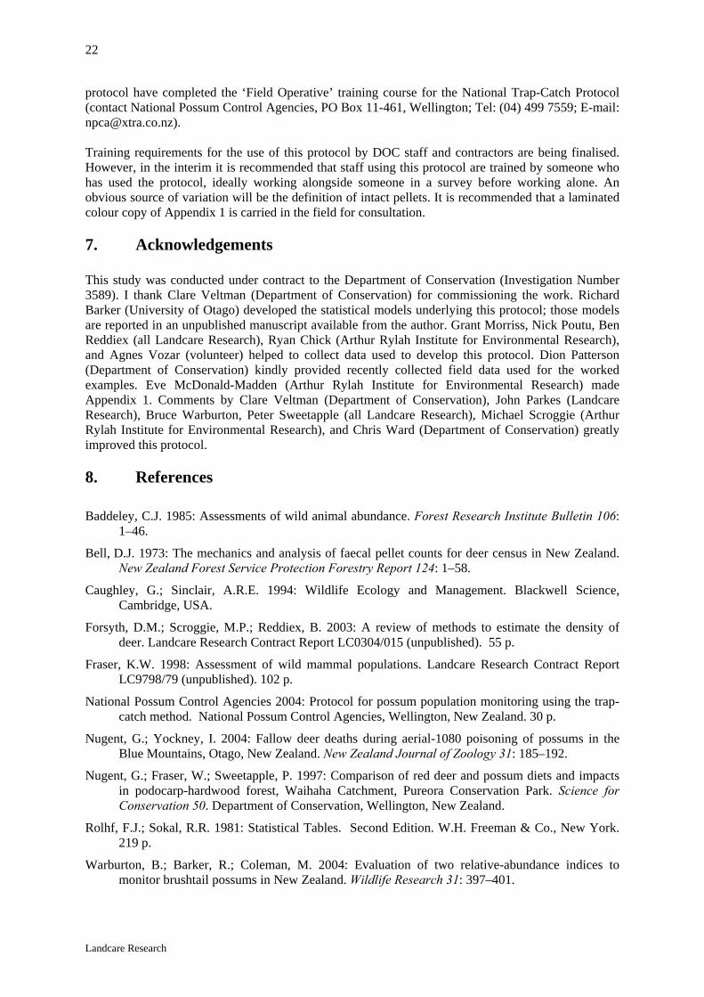
Appendix 1 Definition of intact pellets An intact pellet is defined as having no recognisable loss of material, regardless of whether the pellet is cracked, partly broken or deformed (e.g., by trampling). The presence of moss or fungus does not affect whether a pellet is considered intact or not.

Intact pellets/pellet groups: TO BE RECORDED

Decayed pellets/pellet groups: NOT RECORDED

All pellets intact

Although covered in fungus, all pellets are intact

Although cracked, there no loss of material has occurred

Although discoloured, no loss of material has occurred

There are 3 intact pellets in this clump

All pellets show substantial loss of material

All pellets show loss of material

Cracked and loss of material has occurred

All 4 pellets show loss of material

In each of these 3 masses there are no defined pellets and there has been loss of material

Landcare Research

24

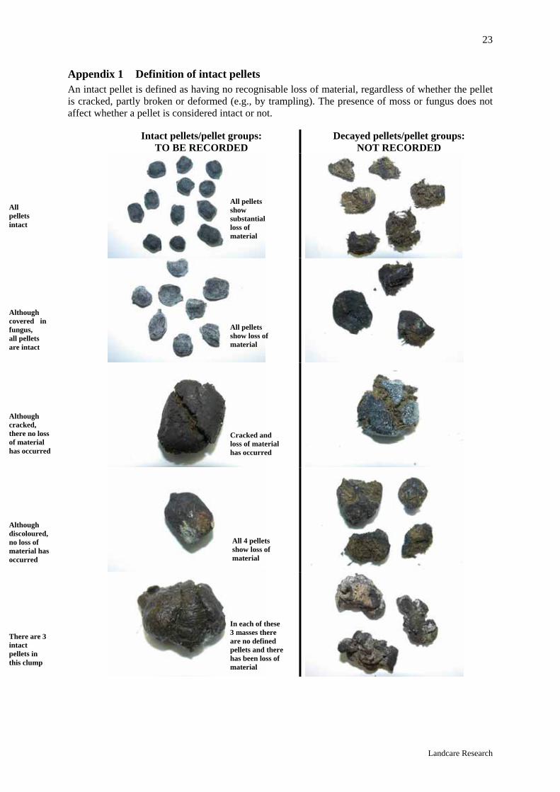
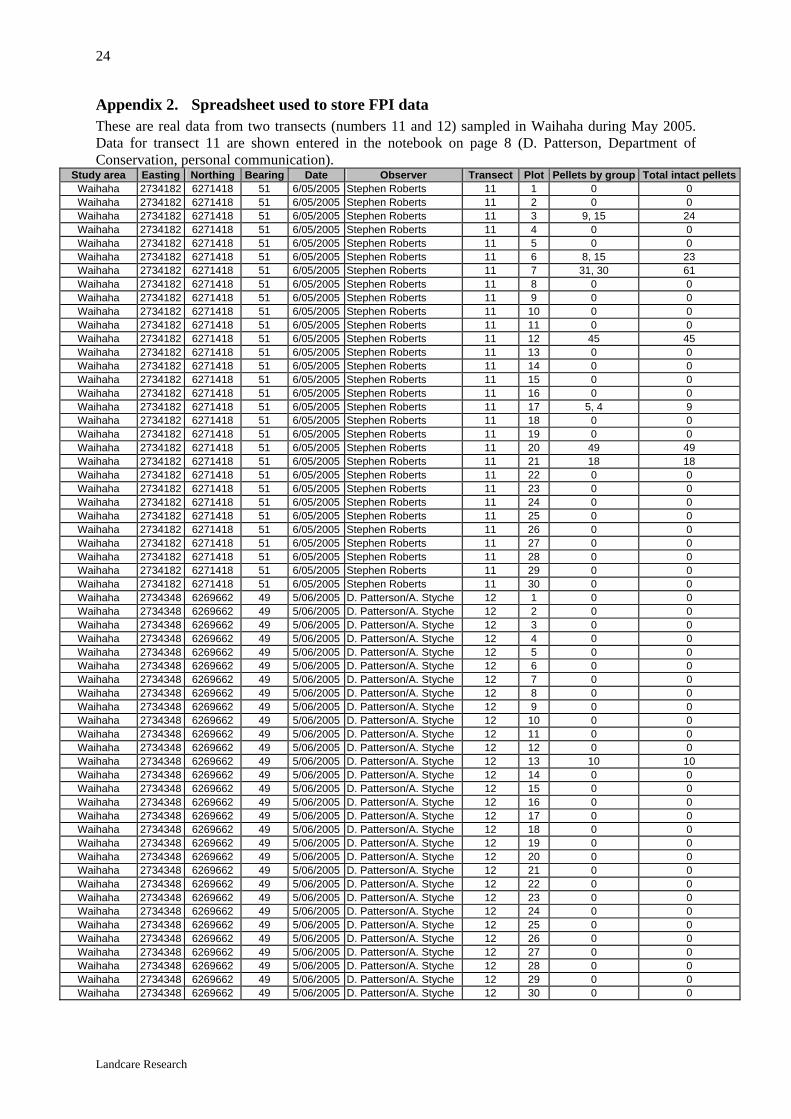
Appendix 2. Spreadsheet used to store FPI data These are real data from two transects (numbers 11 and 12) sampled in Waihaha during May 2005. Data for transect 11 are shown entered in the notebook on page 8 (D. Patterson, Department of Conservation, personal communication).

Study area Easting Northing Bearing Date Observer Transect Plot Pellets by group Total intact pelletsWaihaha 2734182 6271418 51 6/05/2005 Stephen Roberts 11 1 0 0 Waihaha 2734182 6271418 51 6/05/2005 Stephen Roberts 11 2 0 0 Waihaha 2734182 6271418 51 6/05/2005 Stephen Roberts 11 3 9, 15 24 Waihaha 2734182 6271418 51 6/05/2005 Stephen Roberts 11 4 0 0 Waihaha 2734182 6271418 51 6/05/2005 Stephen Roberts 11 5 0 0 Waihaha 2734182 6271418 51 6/05/2005 Stephen Roberts 11 6 8, 15 23 Waihaha 2734182 6271418 51 6/05/2005 Stephen Roberts 11 7 31, 30 61 Waihaha 2734182 6271418 51 6/05/2005 Stephen Roberts 11 8 0 0 Waihaha 2734182 6271418 51 6/05/2005 Stephen Roberts 11 9 0 0 Waihaha 2734182 6271418 51 6/05/2005 Stephen Roberts 11 10 0 0 Waihaha 2734182 6271418 51 6/05/2005 Stephen Roberts 11 11 0 0 Waihaha 2734182 6271418 51 6/05/2005 Stephen Roberts 11 12 45 45 Waihaha 2734182 6271418 51 6/05/2005 Stephen Roberts 11 13 0 0 Waihaha 2734182 6271418 51 6/05/2005 Stephen Roberts 11 14 0 0 Waihaha 2734182 6271418 51 6/05/2005 Stephen Roberts 11 15 0 0 Waihaha 2734182 6271418 51 6/05/2005 Stephen Roberts 11 16 0 0 Waihaha 2734182 6271418 51 6/05/2005 Stephen Roberts 11 17 5, 4 9 Waihaha 2734182 6271418 51 6/05/2005 Stephen Roberts 11 18 0 0 Waihaha 2734182 6271418 51 6/05/2005 Stephen Roberts 11 19 0 0 Waihaha 2734182 6271418 51 6/05/2005 Stephen Roberts 11 20 49 49 Waihaha 2734182 6271418 51 6/05/2005 Stephen Roberts 11 21 18 18 Waihaha 2734182 6271418 51 6/05/2005 Stephen Roberts 11 22 0 0 Waihaha 2734182 6271418 51 6/05/2005 Stephen Roberts 11 23 0 0 Waihaha 2734182 6271418 51 6/05/2005 Stephen Roberts 11 24 0 0 Waihaha 2734182 6271418 51 6/05/2005 Stephen Roberts 11 25 0 0 Waihaha 2734182 6271418 51 6/05/2005 Stephen Roberts 11 26 0 0 Waihaha 2734182 6271418 51 6/05/2005 Stephen Roberts 11 27 0 0 Waihaha 2734182 6271418 51 6/05/2005 Stephen Roberts 11 28 0 0 Waihaha 2734182 6271418 51 6/05/2005 Stephen Roberts 11 29 0 0 Waihaha 2734182 6271418 51 6/05/2005 Stephen Roberts 11 30 0 0 Waihaha 2734348 6269662 49 5/06/2005 D. Patterson/A. Styche 12 1 0 0 Waihaha 2734348 6269662 49 5/06/2005 D. Patterson/A. Styche 12 2 0 0 Waihaha 2734348 6269662 49 5/06/2005 D. Patterson/A. Styche 12 3 0 0 Waihaha 2734348 6269662 49 5/06/2005 D. Patterson/A. Styche 12 4 0 0 Waihaha 2734348 6269662 49 5/06/2005 D. Patterson/A. Styche 12 5 0 0 Waihaha 2734348 6269662 49 5/06/2005 D. Patterson/A. Styche 12 6 0 0 Waihaha 2734348 6269662 49 5/06/2005 D. Patterson/A. Styche 12 7 0 0 Waihaha 2734348 6269662 49 5/06/2005 D. Patterson/A. Styche 12 8 0 0 Waihaha 2734348 6269662 49 5/06/2005 D. Patterson/A. Styche 12 9 0 0 Waihaha 2734348 6269662 49 5/06/2005 D. Patterson/A. Styche 12 10 0 0 Waihaha 2734348 6269662 49 5/06/2005 D. Patterson/A. Styche 12 11 0 0 Waihaha 2734348 6269662 49 5/06/2005 D. Patterson/A. Styche 12 12 0 0 Waihaha 2734348 6269662 49 5/06/2005 D. Patterson/A. Styche 12 13 10 10 Waihaha 2734348 6269662 49 5/06/2005 D. Patterson/A. Styche 12 14 0 0 Waihaha 2734348 6269662 49 5/06/2005 D. Patterson/A. Styche 12 15 0 0 Waihaha 2734348 6269662 49 5/06/2005 D. Patterson/A. Styche 12 16 0 0 Waihaha 2734348 6269662 49 5/06/2005 D. Patterson/A. Styche 12 17 0 0 Waihaha 2734348 6269662 49 5/06/2005 D. Patterson/A. Styche 12 18 0 0 Waihaha 2734348 6269662 49 5/06/2005 D. Patterson/A. Styche 12 19 0 0 Waihaha 2734348 6269662 49 5/06/2005 D. Patterson/A. Styche 12 20 0 0 Waihaha 2734348 6269662 49 5/06/2005 D. Patterson/A. Styche 12 21 0 0 Waihaha 2734348 6269662 49 5/06/2005 D. Patterson/A. Styche 12 22 0 0 Waihaha 2734348 6269662 49 5/06/2005 D. Patterson/A. Styche 12 23 0 0 Waihaha 2734348 6269662 49 5/06/2005 D. Patterson/A. Styche 12 24 0 0 Waihaha 2734348 6269662 49 5/06/2005 D. Patterson/A. Styche 12 25 0 0 Waihaha 2734348 6269662 49 5/06/2005 D. Patterson/A. Styche 12 26 0 0 Waihaha 2734348 6269662 49 5/06/2005 D. Patterson/A. Styche 12 27 0 0 Waihaha 2734348 6269662 49 5/06/2005 D. Patterson/A. Styche 12 28 0 0 Waihaha 2734348 6269662 49 5/06/2005 D. Patterson/A. Styche 12 29 0 0 Waihaha 2734348 6269662 49 5/06/2005 D. Patterson/A. Styche 12 30 0 0