Neurocomputing 193 (2016) 201–212

Contents lists available at ScienceDirect

Neurocomputing

http://d0925-23

n CorrE-m

journal homepage: www.elsevier.com/locate/neucom

Protein–protein interaction sites prediction by ensembling SVMand sample-weighted random forests

Zhi-Sen Wei a, Ke Han a, Jing-Yu Yang a, Hong-Bin Shen b, Dong-Jun Yu a,n

a School of Computer Science and Engineering, Nanjing University of Science and Technology, Xiaolingwei 200, Nanjing 210094, Chinab Institute of Image Processing and Pattern Recognition, Shanghai Jiao Tong University, Dongchuan Road 800, Shanghai 200240, China

a r t i c l e i n f o

Article history:Received 1 December 2015Received in revised form28 January 2016Accepted 10 February 2016

Communicated by: L. Kurgan

(SSWRF) was proposed to deal with class imbalance. An SVM classifier was trained and applied to

Available online 22 February 2016

Keywords:Protein–protein interaction sitesSequence-based predictionImbalanced learningSupport vector machineRandom forestsClassifier ensemble

x.doi.org/10.1016/j.neucom.2016.02.02212/& 2016 Elsevier B.V. All rights reserved.

esponding author. Tel.: þ86 25 84316190; faxail address: njyudj@njust.edu.cn (D.-J. Yu).

a b s t r a c t

Predicting protein–protein interaction (PPI) sites from protein sequences is still a challenge task incomputational biology. There exists a severe class imbalance phenomenon in predicting PPI sites, whichleads to a decrease in overall performance for traditional statistical machine-learning-based classifiers,such as SVM and random forests. In this study, an ensemble of SVM and sample-weighted random forests

estimate the weights of training samples. Then, the training samples with estimated weights were uti-lized to train a sample-weighted random forests (SWRF). In addition, a lower-dimensional featurerepresentation method, which consists of evolutionary conservation, hydrophobic property, solventaccessibility features derived from a target residue and its neighbors, was developed to improve thediscriminative capability for PPI sites prediction. The analysis of feature importance shows that theproposed feature representation method is an effective representation for predicting PPI sites. Theproposed SSWRF achieved 22.4% and 35.1% in MCC and F-measure, respectively, on independent vali-dation dataset Dtestset72, and achieved 15.2% and 36.5% in MCC and F-measure, respectively, onPDBtestset164. Computational comparisons between existing PPI sites predictors on benchmark datasetsdemonstrated that the proposed SSWRF is effective for PPI sites prediction and outperforms the state-of-the-art sequence-based method (i.e., LORIS) released most recently. The benchmark datasets used in thisstudy and the source codes of the proposed method are publicly available at http://csbio.njust.edu.cn/bioinf/SSWRF for academic use.

& 2016 Elsevier B.V. All rights reserved.

1. Introduction

Protein–protein interactions are fundamental for proteins toperform their functions in the living cells, such as catalysis inbiochemical reactions, conformations of the structure of cells andtissues, and the control of cellular processes [1–3]. The interactionsites between proteins are composed of a set of amino acid resi-dues that form a chemical bond with part of another molecule. Theidentification of protein–protein interaction (PPI) sites can assistmany biology applications such as protein docking [4,5], identifi-cation of hot-spot residues [6,7], understanding of disease patho-geny [8,9], and the development of new therapeutic drugs [10–12].

Experimentally identifying protein–protein interaction sites islabor-intensive and time-consuming, and is limited in its ability toidentify interaction sites for transient complexes [13]. With therapidly accumulated sequenced proteins, it is highly desired to

: þ86 25 84315960.

develop computational methods to identify protein–proteininteraction sites from protein sequences. Machine learning tech-niques have been demonstrated to be cost-effective tools forcomputationally predicting protein–protein interaction sites and aseries of PPI sites prediction methods have been developed[14–24].

According to the features used, existing methods for predictingPPI sites can be roughly divided into three groups, i.e., structure-based methods, sequence-based methods, and hybrid methodsutilizing both structural and sequential information. Comparedwith the number of known protein sequences, the number ofproteins with known 3D structures is still considerably small. Thisrestricts the application of methods that use structural informa-tion. On account of this, many researchers have paid much moreattention to develop PPI sites predictors solely from proteinsequences.

During the past decades, several sequence-based methods havebeen developed. As early as 2001, Zhou and Shan [19] proposed aPPI sites prediction method by training a neural network from the

Z.-S. Wei et al. / Neurocomputing 193 (2016) 201–212202

sequence profiles of neighboring residues and solvent exposure;Ofran and Rost [25] have found that the interaction residues tendto be clustered in consecutive sequences. Based on this observa-tion, they trained a predictor called ISIS [20], which is a neuralnetwork based on protein evolutionary information and the pre-dicted structural features within a sub-sequence of nine residues;Porollo and Meller [21] developed a predictor SPPIDER using SVMsand neural networks based on relative solvent accessibility (RSA)and other experimentally selected features from sequences. Theyempirically found out that RSA is a better feature for predicting PPIsites than evolutionary conservation, physicochemical character-istics and structure-derived features; Chen and Jeong [26] pro-posed an integrative ensemble method with random forests basedon several features extracted from protein sequences; Deng et al.[27] trained several SVMs with interaction sites and bootstrappednon-interaction sites and combined them as a final classifier;Murakami and Mizuguchi [22] proposed a new method PSIVER,which trained a naïve Bayesian classifier with kernel densityestimation based on position-specific scoring matrix (PSSM) andpredicted accessibility (PA), for predicting PPI sites; Chen et al. [28]cleaned training data by detecting outlier residues and trained anSVM ensemble based on an encoding schema integrating hydro-phobic scale and sequence profile; More recently, Dhole et al.developed two predictors, SPRINGS [24] and LORIS [23], by train-ing artificial neural networks and L1-regularized logistic regres-sion based on PSSM, averaged cumulative hydropathy (ACH) andpredicted relative solvent accessibility (PRSA).

Although much progress has been made, there still has roomfor further improving the performance of PPI sites prediction,which motivates us to carry out the study presented in this paper.One of the most challenging issues in PPI sites prediction is thereexists a severe class imbalance phenomenon, which may lead todeterioration in the overall performance for those traditional sta-tistical machine-learning-based classifiers such as SVM and ran-dom forests (RF) [29–32].

Existing solutions for class imbalance problem can be groupedinto three categories, sampling-based methods [33–35], learning-based methods (e.g., cost-sensitive learning [36,37], active learn-ing [38], kernel learning [39], and so on) and hybrid methods[40,41] combining both sampling and learning methods. In thisstudy, we aim to address the class imbalance problem in PPI sitesprediction by proposing a new learning-based method. The pro-posed method called SSWRF ensembles an SVM and a sample-weighted random forests (SWRF) to deal with class imbalance.More specifically, we first train an SVM on a given training dataset;then, the trained SVM is used to evaluate the score of each samplein the training dataset; after that, the scores of samples are used tocalculate sample weights, which will be further utilized fortraining an SWRF; finally, the SVM and SWRF are ensembled forpredicting query inputs. In essence, the proposed method is acombination of cost-sensitive learning and ensemble learning.

We evaluated the proposed SSWRF on several PPI sitesbenchmark datasets with a low-dimensional feature set wedeveloped in this study. Computational experiments over strin-gent cross-validation tests and independent validation testsdemonstrate that the proposed SSWRF outperformed the state-of-the-art sequence-based PPI sites prediction methods.

2. Materials and methods

2.1. Benchmark datasets

To carry out evaluations on algorithms for PPI sites prediction,three publicly available benchmark datasets were utilized. Twodatasets developed by Murakami and Mizuguchi [22], denoted as

Dset186 and Dtestset72, were used as the training dataset and thecorresponding independent validation dataset, respectively. Thethird dataset developed by Dhole et al. [23], denoted as PDBtest-set164, was taken as the second independent validation dataset.

The training dataset Dset186 consists of 186 heterodimeric,non-transmembrane, transient protein chains at a resolution ofr3.0 Å extracted from protein data bank (PDB) [42]. The sequenceidentities between any two sequences within the dataset are lessthan 25% to ensure non-redundancy. More details of the con-structing process can be found in the related Ref. [22].

The two independent validation datasets are Dtestset72 andPDBtestset164. The Dtestset72 consists of 72 sequence chains from36 protein complexes in the protein–protein docking benchmarkset version 3.0 [43]. These sequences are non-homologous withany sequence in Dset186 with sequence identity o25% [44]. Basedon the degree of conformation change, the 36 proteins are dividedinto three groups, rigid body cases (27 complexes), medium cases(6 complexes) and difficult cases (3 complexes). The PDBtestset164is composed of 164 non-redundant protein sequences from PDBreleased from June 2010 to November 2013 with the same filters asthat used in constructing Dset186 and Dtestset72.

A residue was defined as an interacting residue if the lostabsolute solvent accessibility on complex formation was morethan 1.0 Å2 [45]. According to this definition, the software PSAIA[46] was utilized to identify interacting residues based on proteinstructure information. As a result, 5517 interacting residues wereidentified from 36,219 residues in Dset186, 1923 interacting resi-dues from 18,140 residues in Dtestset72 and 6096 interactingresidues from 33,681 residues in PDBtestset164. Clearly, both thetraining dataset and the validation datasets exhibit severe classimbalance phenomenon.

2.2. Performance assessment and validation procedure

2.2.1. Performance assessmentThe following six routinely used indexes were taken to perform

performance evaluation:

Recall¼ TP=ðTPþFNÞ ð1Þ

Precision¼ TP=ðTPþFPÞ ð2Þ

Specif icity¼ TN=ðTNþFPÞ ð3Þ

Accuracy¼ ðTPþTNÞ=ðTPþTNþFPþFNÞ ð4Þ

MCC ¼ ððTP � TNÞ�ðFP�FNÞÞ=

ffiffiffiffiffiffiffiffiffiffiffiffiffiffiffiffiffiffiffiffiffiffiffiffiffiffiffiffiffiffiffiffiffiffiffiffiffiffiffiffiffiffiffiffiffiffiffiffiffiffiffiffiffiffiffiffiffiffiffiffiffiffiffiffiffiffiffiffiffiffiffiffiffiffiffiffiffiffiffiffiffiffiffiffiffiffiffiffiffiffiffiffiffiffiffiffiffiðTPþFPÞ � ðTPþFNÞ � ðTNþFPÞ � ðTNþFNÞ

pð5Þ

F�measure¼ 2� ðRecall� PrecisionÞ=ðRecallþPrecisionÞ ð6Þwhere, TP means true positives that are correctly predictedinteracting residues, FP means false positives that are incorrectlypredicted non-interacting residues, TN means true negatives thatare correctly predicted non-interacting residues, FN means falsenegatives that are incorrectly predicted interacting residues.

Among the six indexes, MCC and F�measure are the mostimportant ones to assess and compare the performance of meth-ods because they measure the overall performance of a method.MCC represents the Matthews correlation coefficient [47] thatgives the correlation between prediction and observation for thebinary classification. F�measure [48] is the harmonic mean of Recall and Precision which combines Recall and Precision withbalanced weights.

Besides the above scalar indexes, the receiver operating char-acteristic (ROC) curves are also drawn for comparing differentmethods. The area under the ROC curve (AUC) gives a threshold-

Z.-S. Wei et al. / Neurocomputing 193 (2016) 201–212 203

independent evaluation on the overall performance of a methodfor binary classification.

2.2.2. Validation procedureTo rigorously compare our method with existing PPI sites

prediction methods, both leave-one-out cross-validation andindependent validation were carried out as did by the relatedwork [22–24].

Firstly, the leave-one-out cross-validation was performed onthe training dataset Dset186. More specially, one of the 186sequences was used as the validation set, while the remains wereused as the training set. This process was repeated 186 times tomake each sequence as the validation set once. The average on allvalidation sequences was calculated for each index.

Secondly, the independent validation was carried out onDtestset72 and PDBtestset164. The model trained using Dset186was tested on Dtestset72 and PDBtestset164 with the samethreshold, respectively. Each sequence was tested independentlyand average indexes on all sequences were reported.

Please be noted, we identified the threshold that maximizes thevalue of MCC over leave-one-out cross-validation on Dset186.Then the identified threshold was used to perform independentvalidation tests on both Dtestset72 and PDBtestset164.

2.3. Features extracted from protein sequences

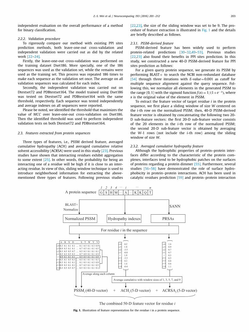
Three types of features, i.e., PSSM derived feature, averagedcumulative hydropathy (ACH) and averaged cumulative relativesolvent accessibility (ACRSA) were used in this study [23]. Previousstudies have shown that interacting residues exhibit aggregationto some extent [25]. In other words, the probability for being aninteracting one of a residue will be high if it is close to an inter-acting residue. In view of this, sliding window technique is used tointroduce neighborhood information for extracting the above-mentioned three types of features. Following previous studies

G S H M … A …1 2 3 4 … i

A protein sequence

BLAST+Normalize

Normalized PSSM Hydropathy in

For residue i in th

0.3 0.1 0.1 0.1 … 0.1 0.5 0.1 0.3 0.90.9 0.3 0.1 0.1 … 0.7 0.5 0.1 0.1 0.50.3 0.5 0.5 0.7 … 0.5 0.3 0.1 0.1 0.10.5 0.3 0.5 0.3 … 0.7 0.9 0.1 0.1 0.50.9 0.1 0.1 0.1 … 0.5 0.5 0.1 0.1 0.90.5 0.1 0.5 0.3 … 0.5 0.1 0.1 0.1 0.10.3 0.1 0.1 0.1 … 0.1 0.5 0.1 0.3 0.90.9 0.3 0.1 0.1 … 0.7 0.5 0.1 0.1 0.50.3 0.5 0.5 0.7 … 0.5 0.3 0.1 0.1 0.1

i-4i-3i-2i-1ii+1i+2i+3i+4

A R N D … S T W Y Vi-4i-3i-2i-1ii+1i+2i+3i+4

4.21.8-3.5-0.81.8-3.54.21.6-0.4

Average along each column

PSSMi (40-D vector) ACHi

Average cumu

+

The combined 50-DFig. 1. Illustration of feature representation

[22,23], the size of the sliding window was set to be 9. The pro-cedure of feature extraction is illustrated in Fig. 1 and the detailsare briefly described as follows.

2.3.1. PSSM-derived featurePSSM-derived feature has been widely used to perform

protein-related predictions [30–32,49–53]. Previous studies[22,23] also found their benefits in PPI sites prediction. In thisstudy, we constructed a new 40-D PSSM-derived feature for PPIsites prediction as follows:

For a given query protein sequence, we generate its PSSM byperforming BLASTþ to search the NCBI non-redundant database[54] through three iterations with E-value¼0.001 as cutoff formultiple sequence alignment against the query sequence. Fol-lowing this, we normalize all elements in the generated PSSM tothe range (0, 1) with the sigmoid function f ðxÞ ¼ 1=ð1þe� xÞ, wherex is the original value of the element in PSSM.

To extract the feature vector of target residue i in the proteinsequence, we first place a sliding window of size W centered onthe i-th row on the normalized PSSM; then, 40-D PSSM-derivedfeature vector is obtained by concatenating the following two 20-D sub-feature vectors: the first 20-D sub-feature vector consistsof the 20 elements in the i-th row of the normalized PSSM;the second 20-D sub-feature vector is obtained by averagingthe W-1 rows (not include the i-th row) among the slidingwindow of size W.

2.3.2. Averaged cumulative hydropathy featureAlthough the hydrophilic properties of protein–protein inter-

faces differ according to the characteristic of the protein com-plexes, interfaces tend to be hydrophobic patches on the surfacesof proteins regarding a protein dimmer [55]. Furthermore, severalstudies [56–58] have demonstrated the role of surface hydro-phobicity in protein–protein interactions. ACH has been used incatalytic residues prediction [59] and protein–protein interaction

K K Q Tn…

dexes PRSAs

SANN

e sequence

i-4i-3i-2i-1ii+1i+2i+3i+4

1.60.90.70.70.30.50.80.81.1

(5-D vector) ACRSAi (5-D vector)

lative with window sizes of 1, 3, 5, 7, and 9

+

feature vector for residue ifor the residue i in a protein sequence.

Z.-S. Wei et al. / Neurocomputing 193 (2016) 201–212204

sites prediction [23]. In light of this, the hydropathy index [60],which measures the hydrophilicity and hydrophobicity of a resi-due's side chain, was utilized for PPI sites prediction in this study.

Averaged cumulative hydropathy (ACH) is calculated withhydropathy indexes of a residue and its neighborhood within awindow. For a residue in a protein sequence, its ACH feature vectoris formed by the averaged hydropathy indexes over a window ofvarious sizes centered on the target residue. In this study, the 5-DACH feature vector consists of the five averaged hydropathyindexes over window of sizes of 1, 3, 5, 7 and 9.

2.3.3. Averaged cumulative relative solvent accessibility featureThe solvent accessibility [61] has close relevance to the spatial

arrangement of a protein, the characteristics of residues packing,and the protein–protein interactions. Porollo and Meller [21] haveexperimentally demonstrated that the solvent accessibility plays acritical role in protein–protein interaction sites prediction.

In this study, the solvent accessibility of a residue is evaluatedby the predicted relative solvent accessibility (PRSA) by the onlineserver SANN [62]. The SANN, which is available at http://lee.kias.re.kr/�newton/sann/, predicts three discrete states and a con-tinuous value of solvent accessibility of each residue in a proteinsequence. In this study, we utilized the predicted continuousvalues of residues predicted by SANN. Based on the predictedcontinuous values of residues, a target residue is described by theaveraged cumulative relative solvent accessibility (ACRSA) feature,which consists of the averaged PRSAs over a window of varioussizes centered on the target residue. Similar to ACH feature, wecalculated the 5-D ACRSA feature by varying the sizes of windowfrom 1 to 9 with a step size of 2.

The final feature of a target residue, the dimensionality ofwhich is 50, can be obtained by serially concatenating its 40-DPSSM-derived feature, a 5-D ACH feature and a 5-D ACRSA feature.

2.4. Ensemble of SVM and sample-weighted random forests

2.4.1. Support vector machineSupport vector machine (SVM) [63] is a typical classification

method in pattern recognition, and has been widely applied tobiological applications [31,64,65]. Different from minimizing theempirical risk of the traditional machine learning methods, SVMminimizes the structural risk. SVM finds a hyperplane to maximizethe margin of two classes. More specifically, SVM finds severalsamples as support vectors that lie on the margin and the optimalhyperplane lies on the center between the two class margins. Inthe case of the two classes that cannot be separated linearly, SVMmakes a tradeoff between maximizing the margin and minimizingthe classification error, which is controlled by the penalty

SVM

SWRF

Sample Weights EnQuerySamplex

Training dataset

Step 1

Step 2

Step 3

Fig. 2. The architecture of the proposed SSWRF. The dotted arrows and the solid arrorespectively. Score and Th represent the final score and the threshold, respectively. “þ”

parameter C. Another characteristic of SVM is that it introducesthe kernel function to project data from a low-dimensional spaceto a high-dimensional space. This is to deal with nonlinear clas-sification problem in the low-dimensional space. The parameterset of the kernel function is denoted as Pkernel. How to set theseSVM parameters will be further discussed in subsequent sections.

2.4.2. Random forestsRandom forests (RF) [66] is also a machine learning method

popularly utilized in computational biology fields [67–70]. It is anensemble of trees with the re-sampling method of bagging. Forclassification, RF combines multiple decision trees trained inde-pendently using subsets randomly sampled with replacementfrom the training data. When training a decision tree, each splitfinds a best feature from a small subset randomly selected fromthe feature space. In addition, the trees are generated withoutpost-pruning since each tree is not trained in the whole featurespace and all the training data and does not readily over-fit. Afterall trees are trained, RF takes an average or majority vote from allthe predictions of trees. When training a random forests, threeparameters need to be set, including the number of trees to grow(nTree), the minimum node size to split (minLeaf ) and the numberof variables to select at random for each decision split (mTry).

2.4.3. An ensemble of SVM and sample-weighted random forestsBoth SVM and RF suffer a decrease in overall performance

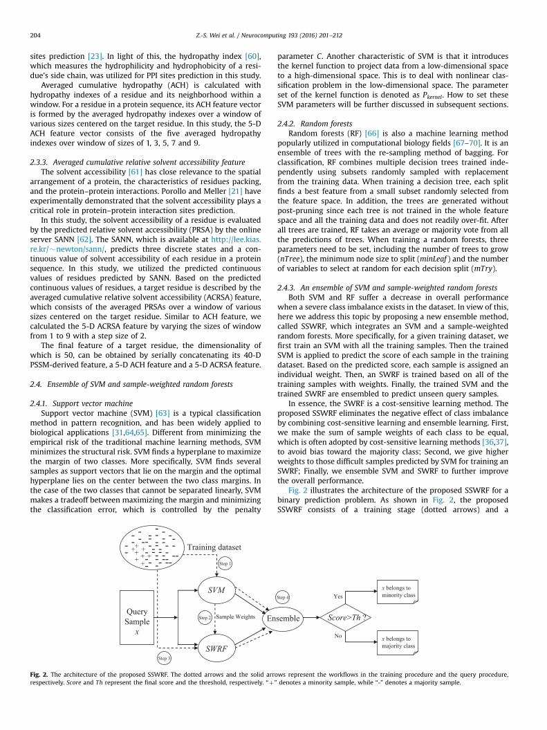
when a severe class imbalance exists in the dataset. In view of this,here we address this topic by proposing a new ensemble method,called SSWRF, which integrates an SVM and a sample-weightedrandom forests. More specifically, for a given training dataset, wefirst train an SVM with all the training samples. Then the trainedSVM is applied to predict the score of each sample in the trainingdataset. Based on the predicted score, each sample is assigned anindividual weight. Then, an SWRF is trained based on all of thetraining samples with weights. Finally, the trained SVM and thetrained SWRF are ensembled to predict unseen query samples.

In essence, the SWRF is a cost-sensitive learning method. Theproposed SSWRF eliminates the negative effect of class imbalanceby combining cost-sensitive learning and ensemble learning. First,we make the sum of sample weights of each class to be equal,which is often adopted by cost-sensitive learning methods [36,37],to avoid bias toward the majority class; Second, we give higherweights to those difficult samples predicted by SVM for training anSWRF; Finally, we ensemble SVM and SWRF to further improvethe overall performance.

Fig. 2 illustrates the architecture of the proposed SSWRF for abinary prediction problem. As shown in Fig. 2, the proposedSSWRF consists of a training stage (dotted arrows) and a

semble Score>Th ?

x belongs tominority class

x belongs tomajority class

Yes

No

Step 4

ws represent the workflows in the training procedure and the query procedure,denotes a minority sample, while “-” denotes a majority sample.

In

O

Z.-S. Wei et al. / Neurocomputing 193 (2016) 201–212 205

prediction stage (solid arrows), details of which will be describedas follows:

2.4.3.1. A. Training stage. Let Dmin and Dmaj be the minority classsample set and the majority class sample set respectively. Asshown in Fig. 2, the training stage of the proposed SSWRF can bedivided into the following 4 steps:

Step 1: Train an SVM model on all training samples

We train an SVM model on the entire training dataset, i.e.Dmin [ Dmaj, with prescribed parameters C and Pkernel. To relievethe negative impact of class imbalance, we can assign a higher costto the minority class and a lower cost to the majority class whentraining an SVM on an imbalance dataset. In this study, we assign1 and Dmaj

�� ��= Dminj j as the costs of the majority and minority clas-ses, respectively, where Uj j represents the cardinality of a set. For agiven input x, the trained SVM will output its scores for belongingto the minority and majority classes. In this study, the score forbelonging to the minority class of a sample, denoted as SVMðxÞ, istaken.

Step 2: Calculate sample weights for all samples

Once an SVM model was trained, each of training samples is re-fed to the trained SVM and a corresponding score, denoted asSVMðxÞ, ranging in [0, 1] is obtained. According to these scores, alltraining samples are assigned weights. More specifically, we definesample weight function for minority class sample as follows:

WminðxÞ ¼1

Dmin�� ���

11þescale�ðSVMðxÞ�maxnsÞ ð7Þ

The sample weight function for majority class sample is definedas follows:

WmajðxÞ ¼1

Dmaj�� ���

11þescale�ðminps�SVMðxÞÞ ð8Þ

where, x means a sample, SVMðxÞ means the score of a samplex predicted by the trained SVM, Uj j is the cardinality of a set,maxns means the maximum score of all majority samples, minps means the minimum score of all minority samples and scale is a parameter to control the distribution of sampleweights.

According to Eq. (7) and Eq. (8), a minority class sample will beassigned a large weight if its SVMðxÞ predicted by SVM is small;while a majority class sample will be assigned a large weight if itsSVMðxÞ is big. Samples assigned with large weights can be con-sidered as “hard” targets for SVM to perform classification, whilesamples assigned with small weights can be considered as “easy”targets. Assigning different weights to samples according to their“hardness” or “easiness” will facilitate the subsequent training ofsample-weighted random forests.

Step 3: Train a sample-weighted random forests

Based on the training dataset Dmin [ Dmaj and the sampleweights obtained in Step 2, we can train an SWRF model. Thetraining procedure of an SWRF is the same as that of a traditionalrandom forests except training each tree with sample weights [71].To train a random forests, three parameters need to be preset,including the number of trees to grow (nTree), the minimum nodesize to split (minLeaf ) and the number of variables to select atrandom for each decision split (mTry). For a given input x, thetrained SWRF will output its scores for belonging to the minorityand majority classes. Similar to the SVM model in Step 1, the score

for belonging to the minority class of a sample predicted by thetrained SWRF, denoted as SWRFðxÞ, is taken.

Step 4: Return the trained SSWRF

Once both SVM and SWRF are trained, the final SSWRF model isachieved by averaging the outputs of SVM and SWRF. For a givenquery sample x, the output of SSWRF, denoted as SSWRFðxÞ, can beformulated as follows:

SSWRFðxÞ ¼ ðSVMðxÞþSWRFðxÞÞ=2 ð9Þ

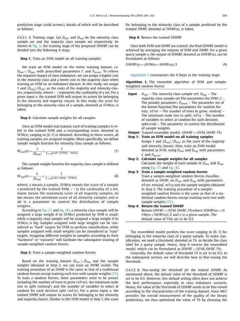
Algorithm 1 summarizes the 4 Steps in the training stage.

Algorithm 1. The ensemble algorithm of SVM and sample-weighted random forests

put

Dmin – The minority class sample set; Dmaj – Themajority class sample set;The parameters for SVM: C –

The penalty parameter; Pkernel – The parameter set ofthe kernel function;The parameters for random for-ests: nTree – The number of trees to grow; minLeaf –

The minimum node size to split; mTry – The numberof variables to select at random for each decisionsplit;scale – The parameter to control the distributionof sample weights.

utput

Trained ensemble model: SSWRF ¼ fSVM; SWRF; Thg tep 1: Train an SVM model on all training samples� � S

Assign 1 and Dmaj� �= Dminj j as the costs of the majority

and minority classes; then, train an SVM model,denoted as SVM, using Dmin and Dmaj with parametersC and Pkernel.

tep 2:

Calculate sample weights for all samples S Calculate the weight of each sample in Dmin and Dmaj

using Eq. (7) and Eq. (8).

tep 3: Train a sample-weighted random forests S

Train a sample-weighted random forests classifier,denoted as SWRF , on Dmin and Dmaj with parametersnTree,minLeaf ,mTry and the sample weights obtainedin Step 2. The training procedure of a sample-weighted random forests is the same as that of a tra-ditional random forests except training each tree withsample weights [71].

tep 4:

Return the trained SSWRF S Return SSWRF ¼ fSVM; SWRF; Thgwhere SSWRFðxÞ ¼ ðSVMðxÞþSWRFðxÞÞ=2 and x is a given sample. Thedefault value of This set to be 0.5.

The ensembled model predicts the score ranging in [0, 1] forbelonging to the minority class of a query sample. To make clas-sification, we need a threshold, denoted as Th, to decide the classlabel for a query sample. Hence, Step 4 returns the ensembledmodel, which can be formulated as SSWRF ¼ fSVM; SWRF; Thg.

Generally, the default value of threshold Th is set to be 0.5. Inthe subsequent section, we will describe how to fine-tuning thethreshold.

2.4.3.2. B. Fine-tuning the threshold for the trained SSWRF. Asmentioned above, the default value of the threshold of SSWRF isset to be 0.5. However, this default setting often does not achievethe best performance, especially in class imbalance scenario.Hence, the value of the threshold of SSWRF needs to be fine-tunedaccording to the characteristics of the training dataset. Since MCCprovides the overall measurement of the quality of the binarypredictions, we thus optimized the value of Th by choosing the

Z.-S. Wei et al. / Neurocomputing 193 (2016) 201–212206

threshold which maximizes the value of MCC of predictions ontraining dataset over leave-one-out cross-validation.

2.4.3.3. C. Prediction stage. For a given query sample x, predictioncan be performed by feeding the sample to the SVMmodel and theSWRF model, respectively, in the trained SSWRF ¼ fSVM;

SWRF; Thg. Then, the scores predicted by the two classifiers areaveraged to get the final score. Based on the final score and thethreshold Th, the class label of the query sample can be deter-mined: if the final score of a query sample is greater than the valueof Th, it will be predicted as minority class; otherwise, it will bepredicted as majority class.

3. Results and discussion

3.1. Parameters configuration

As described in Algorithm 1, there are several parameters needto be prescribed for training the proposed SSWRF. Here, weexplain how to optimize these parameters to achieve betterperformance.

(1) For training an SVM, the penalty parameter C and the kernelfunction Pkernel need to be prescribed. In this study, we train alinear SVM using LIBSVM (v3.20) [72] thus only the penaltyparameter C needs to be optimized. Considering that the AUC givesan evaluation on the overall performance of a prediction model,we thus optimize the value of C regarding the AUC index. More

specifically, we choose the CA 2i j iAΖ ; �10r ir5n o

, which

maximizes the value of AUC of predictions of SVM on trainingdataset Dset186 over leave-one-out cross-validation, where Ζ isthe integer set. After this optimization procedure, the value of C isidentified to be 0.125.

(2) For training an SWRF, the nTree, minLeaf , mTry, and scaleneed to be prescribed. We empirically set nTree¼ 400, minLeaf ¼15 and scale¼ 7 according to our local tests on Dset186 over leave-one-out cross-validation. Then, we further optimize the parametermTry (which is much sensitive to the performance of SWRFcompared with nTree and minLeaf ) regarding the AUC index. Morespecifically, we gradually vary the value of mTry from 1 to 50 witha step size of 1 and the one which maximizes the value of AUC ofthe SWRF on Dset186 over leave-one-out crossing-validation ischosen. As a result, we find mTry¼ 9 corresponds to the maximalvalue of AUC.

(3) As described in Algorithm 1, the default value of Th is set tobe 0.5. We optimize this threshold parameter regarding anotherthreshold-dependent overall performance evaluation index, i.e.,MCC. More specifically, we optimize the value of Th by varying itsvalue from 0 to 1 with a step size of 0.01 and the one, whichachieves the highest value of MCC of predictions of SSWRF onDset186 over leave-one-out crossing-validation, is chosen. In thisstudy, the identified value of Th is 0.31.

Table 1Performance comparisons between the proposed SSWRF, SVMRF, RF, and SVM on datas

Method MCC F-measure Recall (%

SSWRF 0.234 (0.001) 0.386 (0.001) 58.1 (0.1SVMRF 0.217 (0.001) 0.363 (0.001) 50.5 (0.1RF 0.221 (0.002) 0.364 (0.001) 50.6 (0.2SVM 0.201 (0.000) 0.371 (0.000) 62.8 (0.0

n For each method, experiments were performed three times, and the averaged results

3.2. Effectiveness of the proposed SSWRF for dealing with classimbalance

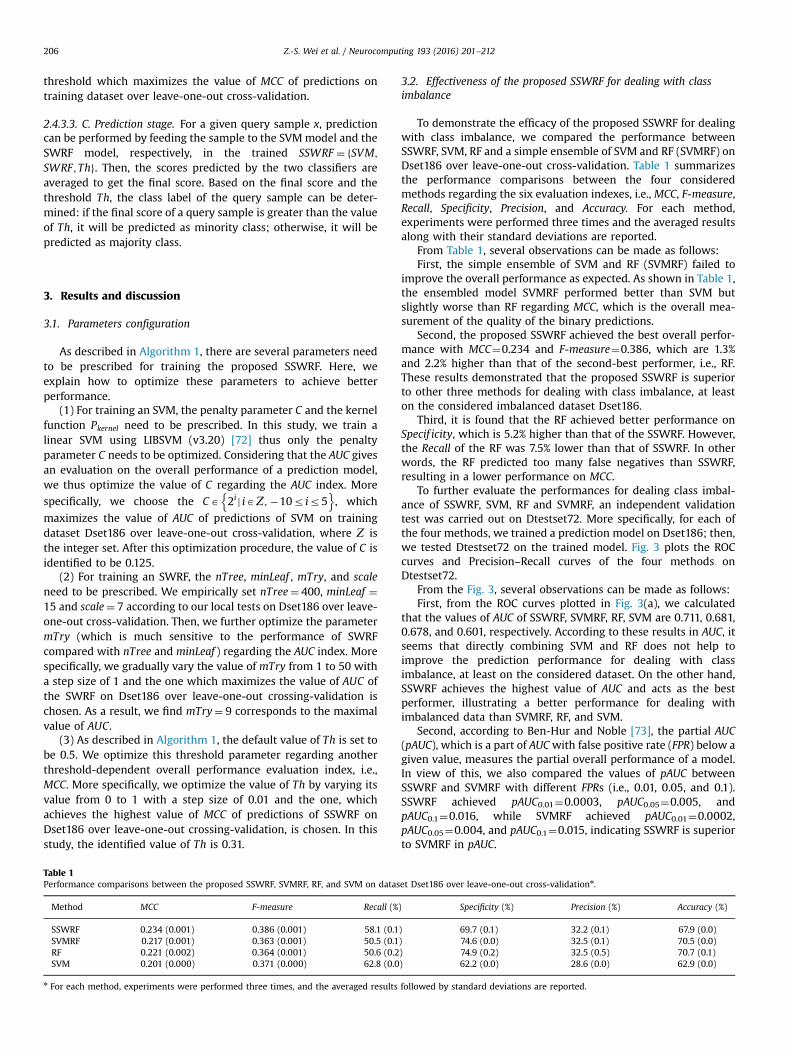
To demonstrate the efficacy of the proposed SSWRF for dealingwith class imbalance, we compared the performance betweenSSWRF, SVM, RF and a simple ensemble of SVM and RF (SVMRF) onDset186 over leave-one-out cross-validation. Table 1 summarizesthe performance comparisons between the four consideredmethods regarding the six evaluation indexes, i.e., MCC, F-measure,Recall, Specificity, Precision, and Accuracy. For each method,experiments were performed three times and the averaged resultsalong with their standard deviations are reported.

From Table 1, several observations can be made as follows:First, the simple ensemble of SVM and RF (SVMRF) failed to

improve the overall performance as expected. As shown in Table 1,the ensembled model SVMRF performed better than SVM butslightly worse than RF regarding MCC, which is the overall mea-surement of the quality of the binary predictions.

Second, the proposed SSWRF achieved the best overall perfor-mance with MCC¼0.234 and F-measure¼0.386, which are 1.3%and 2.2% higher than that of the second-best performer, i.e., RF.These results demonstrated that the proposed SSWRF is superiorto other three methods for dealing with class imbalance, at leaston the considered imbalanced dataset Dset186.

Third, it is found that the RF achieved better performance onSpecif icity, which is 5.2% higher than that of the SSWRF. However,the Recall of the RF was 7.5% lower than that of SSWRF. In otherwords, the RF predicted too many false negatives than SSWRF,resulting in a lower performance on MCC.

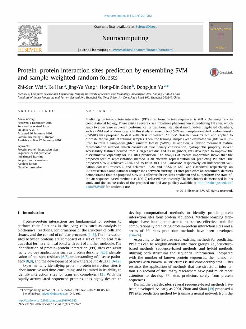
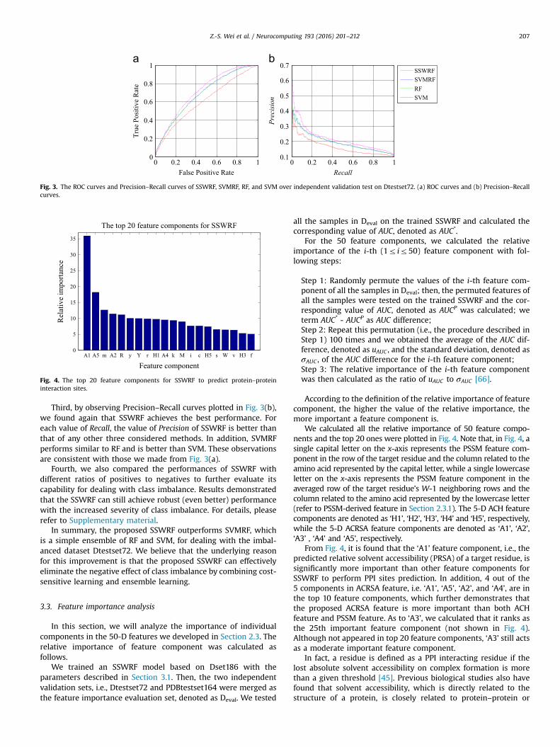
To further evaluate the performances for dealing class imbal-ance of SSWRF, SVM, RF and SVMRF, an independent validationtest was carried out on Dtestset72. More specifically, for each ofthe four methods, we trained a prediction model on Dset186; then,we tested Dtestset72 on the trained model. Fig. 3 plots the ROCcurves and Precision–Recall curves of the four methods onDtestset72.

From the Fig. 3, several observations can be made as follows:First, from the ROC curves plotted in Fig. 3(a), we calculated

that the values of AUC of SSWRF, SVMRF, RF, SVM are 0.711, 0.681,0.678, and 0.601, respectively. According to these results in AUC, itseems that directly combining SVM and RF does not help toimprove the prediction performance for dealing with classimbalance, at least on the considered dataset. On the other hand,SSWRF achieves the highest value of AUC and acts as the bestperformer, illustrating a better performance for dealing withimbalanced data than SVMRF, RF, and SVM.

Second, according to Ben-Hur and Noble [73], the partial AUC(pAUC), which is a part of AUCwith false positive rate (FPR) below agiven value, measures the partial overall performance of a model.In view of this, we also compared the values of pAUC betweenSSWRF and SVMRF with different FPRs (i.e., 0.01, 0.05, and 0.1).SSWRF achieved pAUC0.01¼0.0003, pAUC0.05¼0.005, andpAUC0.1¼0.016, while SVMRF achieved pAUC0.01¼0.0002,pAUC0.05¼0.004, and pAUC0.1¼0.015, indicating SSWRF is superiorto SVMRF in pAUC.

et Dset186 over leave-one-out cross-validationn.

) Specificity (%) Precision (%) Accuracy (%)

) 69.7 (0.1) 32.2 (0.1) 67.9 (0.0)) 74.6 (0.0) 32.5 (0.1) 70.5 (0.0)) 74.9 (0.2) 32.5 (0.5) 70.7 (0.1)) 62.2 (0.0) 28.6 (0.0) 62.9 (0.0)

followed by standard deviations are reported.

A1 A5 m A2 R y Y r H1 A4 k M i c H5 s W v H3 f0

5

10

15

20

25

30

35

Feature component

Rel

ativ

e im

porta

nce

The top 20 feature components for SSWRF

Fig. 4. The top 20 feature components for SSWRF to predict protein–proteininteraction sites.

0 0.2 0.4 0.6 0.8 10

0.2

0.4

0.6

0.8

1

False Positive Rate

True

Pos

itive

Rat

e

SSWRFSVMRFRFSVM

0 0.2 0.4 0.6 0.8 10.1

0.2

0.3

0.4

0.5

0.6

0.7

Recall

Precision

Fig. 3. The ROC curves and Precision–Recall curves of SSWRF, SVMRF, RF, and SVM over independent validation test on Dtestset72. (a) ROC curves and (b) Precision–Recallcurves.

Z.-S. Wei et al. / Neurocomputing 193 (2016) 201–212 207

Third, by observing Precision–Recall curves plotted in Fig. 3(b),we found again that SSWRF achieves the best performance. Foreach value of Recall, the value of Precision of SSWRF is better thanthat of any other three considered methods. In addition, SVMRFperforms similar to RF and is better than SVM. These observationsare consistent with those we made from Fig. 3(a).

Fourth, we also compared the performances of SSWRF withdifferent ratios of positives to negatives to further evaluate itscapability for dealing with class imbalance. Results demonstratedthat the SSWRF can still achieve robust (even better) performancewith the increased severity of class imbalance. For details, pleaserefer to Supplementary material.

In summary, the proposed SSWRF outperforms SVMRF, whichis a simple ensemble of RF and SVM, for dealing with the imbal-anced dataset Dtestset72. We believe that the underlying reasonfor this improvement is that the proposed SSWRF can effectivelyeliminate the negative effect of class imbalance by combining cost-sensitive learning and ensemble learning.

3.3. Feature importance analysis

In this section, we will analyze the importance of individualcomponents in the 50-D features we developed in Section 2.3. Therelative importance of feature component was calculated asfollows.

We trained an SSWRF model based on Dset186 with theparameters described in Section 3.1. Then, the two independentvalidation sets, i.e., Dtestset72 and PDBtestset164 were merged asthe feature importance evaluation set, denoted as Deval. We tested

all the samples in Deval on the trained SSWRF and calculated thecorresponding value of AUC, denoted as AUC*.

For the 50 feature components, we calculated the relativeimportance of the i-th (1r ir50) feature component with fol-lowing steps:

Step 1: Randomly permute the values of the i-th feature com-ponent of all the samples in Deval; then, the permuted features ofall the samples were tested on the trained SSWRF and the cor-responding value of AUC, denoted as AUCP was calculated; weterm AUC* - AUCP as AUC difference;Step 2: Repeat this permutation (i.e., the procedure described inStep 1) 100 times and we obtained the average of the AUC dif-ference, denoted as uAUC , and the standard deviation, denoted asσAUC , of the AUC difference for the i-th feature component;Step 3: The relative importance of the i-th feature componentwas then calculated as the ratio of uAUC to σAUC [66].

According to the definition of the relative importance of featurecomponent, the higher the value of the relative importance, themore important a feature component is.

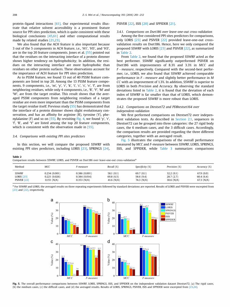
We calculated all the relative importance of 50 feature compo-nents and the top 20 ones were plotted in Fig. 4. Note that, in Fig. 4, asingle capital letter on the x-axis represents the PSSM feature com-ponent in the row of the target residue and the column related to theamino acid represented by the capital letter, while a single lowercaseletter on the x-axis represents the PSSM feature component in theaveraged row of the target residue’s W-1 neighboring rows and thecolumn related to the amino acid represented by the lowercase letter(refer to PSSM-derived feature in Section 2.3.1). The 5-D ACH featurecomponents are denoted as ‘H1’, ‘H2’, ‘H3’, ‘H4’ and ‘H5’, respectively,while the 5-D ACRSA feature components are denoted as ‘A1’, ‘A2’,‘A3’ , ‘A4’ and ‘A5’, respectively.

From Fig. 4, it is found that the ‘A1’ feature component, i.e., thepredicted relative solvent accessibility (PRSA) of a target residue, issignificantly more important than other feature components forSSWRF to perform PPI sites prediction. In addition, 4 out of the5 components in ACRSA feature, i.e. ‘A1’, ‘A5’, ‘A2’, and ‘A4’, are inthe top 10 feature components, which further demonstrates thatthe proposed ACRSA feature is more important than both ACHfeature and PSSM feature. As to ‘A3’, we calculated that it ranks asthe 25th important feature component (not shown in Fig. 4).Although not appeared in top 20 feature components, ‘A3’ still actsas a moderate important feature component.

In fact, a residue is defined as a PPI interacting residue if thelost absolute solvent accessibility on complex formation is morethan a given threshold [45]. Previous biological studies also havefound that solvent accessibility, which is directly related to thestructure of a protein, is closely related to protein–protein or

Z.-S. Wei et al. / Neurocomputing 193 (2016) 201–212208

protein–ligand interactions [61]. Our experimental results illus-trate that relative solvent accessibility is a prominent featuresource for PPI sites prediction, which is quite consistent with thesebiological conclusions [45,61] and other computational resultsmade by related studies [21,23].

We also found that the ACH feature is also important because3 out of the 5 components in ACH feature, i.e., ‘H1’, ‘H5’, and ‘H3’,are in the top 20 feature components. Jones et al. [55] pointed outthat the residues on the interacting interface of a protein dimmershows higher tendency on hydrophobicity; In addition, the resi-dues on the interacting interface are more hydrophobic thanresidues on other protein surfaces. These observations account forthe importance of ACH feature for PPI sites prediction.

As to PSSM feature, we found 13 out of 40 PSSM feature com-ponents are listed in top 20. Among the 13 PSSM feature compo-nents, 9 components, i.e., ‘m’, ‘y’, ‘r’, ‘k’, ‘i’, ‘c’, ‘s’, ‘v’, ‘f’, are fromneighboring residues, while only 4 components, i.e., ‘R’, ‘Y’, ‘M’ and‘W’, are from the target residue. This result shows that the aver-aged PSSM components from neighboring residues of a targetresidue are even more important than the PSSM components fromthe target residue itself. Previous study [55] has demonstrated thatthe interface of a protein dimmer shows slight evolutionary con-servation, and has an affinity for arginine (R), tyrosine (Y), phe-nylalanine (F) and so on [55]. By revisiting Fig. 4, we found ‘y’, ‘r’,‘f’, ‘R’, and ‘Y’ are listed among the top 20 feature components,which is consistent with the observation made in [55].

3.4. Comparisons with existing PPI sites predictors

In this section, we will compare the proposed SSWRF withexisting PPI sites predictors, including LORIS [23], SPRINGS [24],

Table 2Comparison results between SSWRF, LORIS, and PSIVER on Dset186 over leave-one-out

Method MCC F-measure Recall (

SSWRF 0.234 (0.001) 0.386 (0.001) 58.1 (0LORIS [23] 0.221 (0.026) 0.384 (0.014) 69.8 (6PSIVER [22] 0.151 (N/A) 0.353 (N/A) 41.6 (N

n For SSWRF and LORIS, the averaged results on three repeating experiments followed by[23] and [22], respectively.

0

10

20

30

40

Val

ue (%

)

21.7

34.5

17.5

32.0

16.7

31.3

12.7

27.3

11.0

25.9

8.7

24.4

0

10

20

30

40

Val

ue (%

)

0

10

20

30

40

Val

ue (%

)

22.7

38.5

17.4

35.5

14.3

32.8

13.9

33.2

0.1

23.0

7.0

32.7

0

10

20

30

40

Val

ue (%

)

MCC F-measure

F-measureMCC

Fig. 5. The overall performance comparisons between SSWRF, LORIS, SPRINGS, ISIS, an(b) the medium cases, (c) the difficult cases, and (d) the averaged results. Results of LO

PSIVER [22], ISIS [20] and SPPIDER [21].

3.4.1. Comparisons on Dset186 over leave-one-out cross-validationAmong the five considered PPI sites predictors for comparisons,

only LORIS [23] and PSIVER [22] provided leave-one-out cross-validation results on Dset186. Hence, here we only compared theproposed SSWRF with LORIS [23] and PSIVER [22], as summarizedin Table 2.

From Table 2, we found that the proposed SSWRF acted as thebest performer. SSWRF significantly outperformed PSIVER onDset186 with improvements of 8.3% and 3.3% in MCC andF�measure, respectively. Compared with the second-best perfor-mer, i.e., LORIS, we also found that SSWRF achieved comparableperformance in F�measure and slightly better performance in MCC with an improvement of 1.3%. In addition, SSWRF is superior toLORIS in both Precision and Accuracy. By observing the standarddeviations listed in Table 2, it is found that the deviation of eachindex of SSWRF is far smaller than that of LORIS, which demon-strates the proposed SSWRF is more robust than LORIS.

3.4.2. Comparisons on Dtestset72 and PDBtestset164 overindependent-validation

We first performed comparisons on Dtestset72 over indepen-dent validation tests. As described in Section 2.1, sequences inDtestset72 can be grouped into three categories: the 27 rigid bodycases, the 6 medium cases, and the 3 difficult cases. Accordingly,the comparison results are provided regarding the three differentcategories, together with an averaged result.

Fig. 5 illustrates the comparisons of the overall performancemeasured byMCC and F-measure between SSWRF, LORIS, SPRINGS,ISIS, and SPPIDER, while Table 3 summarizes comparisons

cross-validationn.

%) Specificity (%) Precision (%) Accuracy (%)

.1) 69.7 (0.1) 32.2 (0.1) 67.9 (0.0)

.5) 58.6 (9.4) 28.7 (2.7) 60.4 (6.4)/A) 74.3 (N/A) 30.6 (N/A) 67.3 (N/A)

standard deviations are reported. Results of LORIS and PSIVER were excerpted from

SSWRFLORISSPRINGSPSIVERISISSPPIDER

25.1

36.1

18.7

32.9

19.7

33.7

17.1

27.1

5.0

19.0

5.5

18.4

22.4

35.1

17.7

32.4

17.0

31.8

13.5

27.8

9.1

24.5

8.1

24.1

MCC

MCC

F-measure

F-measure

d SPPIDER on the independent validation dataset Dtestset72. (a) The rigid cases,RIS, SPRINGS, PSIVER, ISIS and SPPIDER were excerpted from [23,24].

Z.-S. Wei et al. / Neurocomputing 193 (2016) 201–212 209

between these methods regarding Recall, Specificity, Precision, andAccuracy.

As shown in Fig. 5(a), (b), and (c), the proposed SSWRF out-performed five other related popular PPI sites predictors in eachsubcategory. Compared with the most recently released LORIS,which acted as the second-best performer, SSWRF achievedimprovements of 4.2%, 6.4% and 5.3% in MCC and 2.5%, 3.2% and3.0% in F�measure for rigid body case, medium case, and difficultcase, respectively. In addition, the averaged values of MCC and F-measure of SSWRF are 22.4% and 35.1%, which are 4.7% and 2.7%better than that of LORIS (refer to Fig. 5(d)).

From the averaged performance listed in Table 3, it is foundthat ISIS and PSIVER often performed best concerning Specificityand Accuracy. By carefully analyzing the results listed in Table 3,we found that the values of Recall of these two methods are sig-nificantly lower than that of SSWRF and LORIS. To further fairlycompare the performances of the six considered predictors, wecompared the Recall values of the six predictors at the equal Spe-cificity value by changing a threshold value for each method.Considering that currently the websites of ISIS and SPPIDER do notwork, we only compared performances under given Specificityvalue between SSWRF, LORIS, SPRINGS, and PSIVER. We computed

Table 3The performance comparisons between SSWRF, LORIS, SPRINGS, ISIS, and SPPIDERon the independent validation dataset Dtestset72n.

Method Recall (%) Specificity (%) Precision (%) Accuracy (%)

Rigid body cases (27)SSWRF 66.2 63.0 25.7 63.9LORIS [23] 63.8 60.3 23.2 60.9SPRINGS [24] 59.2 62.5 23.5 62.1PSIVER [22] 46.5 68.8 23.9 65.5ISIS [20] 37.9 75.7 22.0 70.9SPPIDER [21] 44.7 65.2 20.4 62.9Medium cases (6)SSWRF 66.7 65.3 28.6 65.9LORIS [23] 60.9 63.4 25.0 63.3SPRINGS [24] 59.1 65.6 26.2 64.9PSIVER [22] 43.5 75.3 28.9 70.2ISIS [20] 23.0 82.6 18.4 75.2SPPIDER [21] 36.1 68.4 19.4 62.7Difficult cases (3)SSWRF 55.0 73.8 31.7 69.8LORIS [23] 61.1 62.7 26.5 61.8SPRINGS [24] 57.7 62.3 24.9 60.3PSIVER [22] 53.2 61.9 26.9 62.8ISIS [20] 33.5 67.7 17.8 62.4SPPIDER [21] 70.4 41.3 22.1 49.3Averaged performance (72)SSWRF 65.4 64.3 26.7 64.8LORIS [23] 63.1 61.0 23.8 61.4SPRINGS [24] 59.0 63.0 24.1 62.4PSIVER [22] 46.5 69.3 25.0 66.1ISIS [20] 35.0 76.2 21.0 70.9SPPIDER [21] 45.4 63.7 20.4 61.7

n Results of LORIS, SPRINGS, PSIVER, ISIS, and SPPIDER were excerpted from [23,24].

Table 4The comparisons between the proposed SSWRF and LORIS, SPRINGS, PSIVER, and SPPID

Method MCC F-measure Recall (%)

SSWRF 0.152 0.365 52.7LORIS [23] 0.111 0.323 53.8SPRINGS [24] 0.108 0.311 40.7PSIVER [22] 0.078 0.295 46.4SPPIDER [21] 0.015 0.129 16.2

n Results of LORIS, SPRINGS, PSIVER were excerpted from [23,24]. Results of SPPIDER we[21].

that the Recall values of SSWRF, LORIS, SPRINGS, and PSIVER are58.8%, 54.0%, 45.1%, and 46.5%, respectively, when the Specificityvalue is set to be 69.3%. The above observations demonstrate thatthe proposed SSWRF can achieve much higher true positive rateunder the same false positive rate (or true negative rate), leadingto a superior overall performance on MCC and F-measure.

The comparison results on PDBtestset164 are listed in Table 4.Again, we found that the proposed SSWRF achieved the bestperformance on PDBtestset164 with the highest values of all thesix considered evaluation indexes except for the Accuracy. Thevalues of MCC and F-measure of SSWRF are 4.1% and 4.2%,respectively, better than that of LORIS, and are significantly largerthan that of SPPIDER, PSIVER, and SPRINGS.

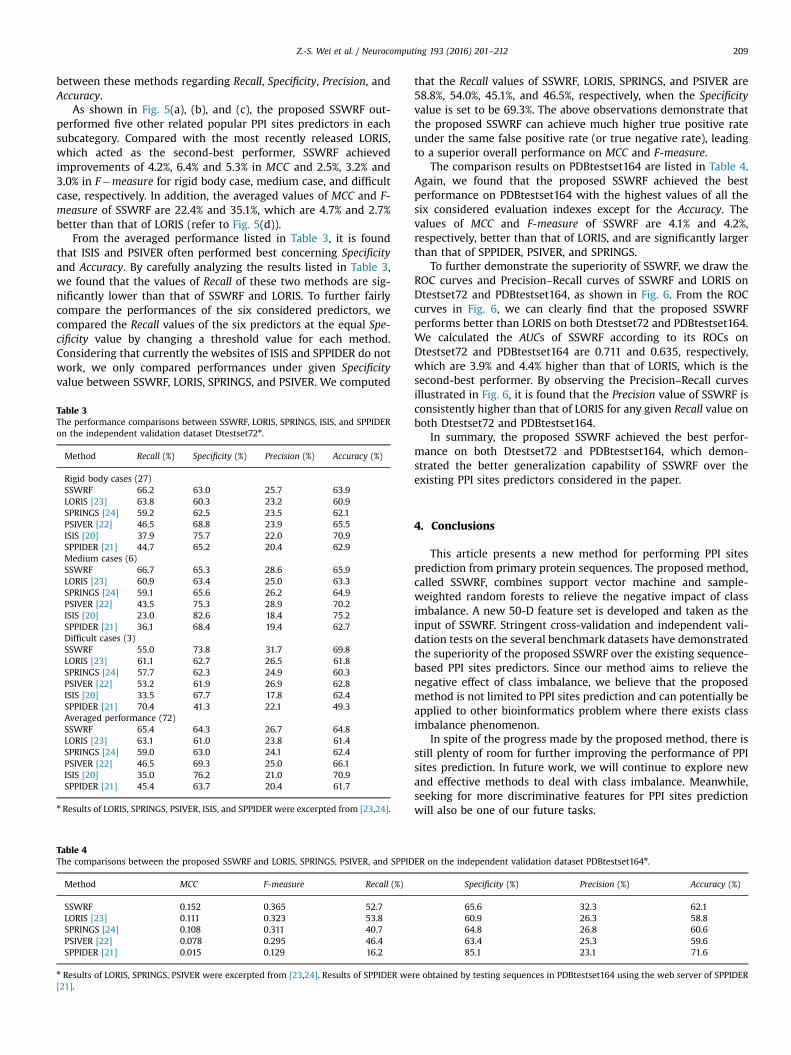
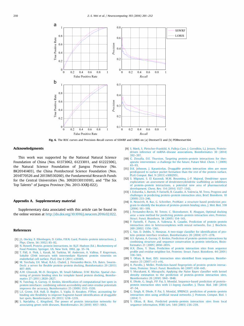
To further demonstrate the superiority of SSWRF, we draw theROC curves and Precision–Recall curves of SSWRF and LORIS onDtestset72 and PDBtestset164, as shown in Fig. 6. From the ROCcurves in Fig. 6, we can clearly find that the proposed SSWRFperforms better than LORIS on both Dtestset72 and PDBtestset164.We calculated the AUCs of SSWRF according to its ROCs onDtestset72 and PDBtestset164 are 0.711 and 0.635, respectively,which are 3.9% and 4.4% higher than that of LORIS, which is thesecond-best performer. By observing the Precision–Recall curvesillustrated in Fig. 6, it is found that the Precision value of SSWRF isconsistently higher than that of LORIS for any given Recall value onboth Dtestset72 and PDBtestset164.

In summary, the proposed SSWRF achieved the best perfor-mance on both Dtestset72 and PDBtestset164, which demon-strated the better generalization capability of SSWRF over theexisting PPI sites predictors considered in the paper.

4. Conclusions

This article presents a new method for performing PPI sitesprediction from primary protein sequences. The proposed method,called SSWRF, combines support vector machine and sample-weighted random forests to relieve the negative impact of classimbalance. A new 50-D feature set is developed and taken as theinput of SSWRF. Stringent cross-validation and independent vali-dation tests on the several benchmark datasets have demonstratedthe superiority of the proposed SSWRF over the existing sequence-based PPI sites predictors. Since our method aims to relieve thenegative effect of class imbalance, we believe that the proposedmethod is not limited to PPI sites prediction and can potentially beapplied to other bioinformatics problem where there exists classimbalance phenomenon.

In spite of the progress made by the proposed method, there isstill plenty of room for further improving the performance of PPIsites prediction. In future work, we will continue to explore newand effective methods to deal with class imbalance. Meanwhile,seeking for more discriminative features for PPI sites predictionwill also be one of our future tasks.

ER on the independent validation dataset PDBtestset164n.

Specificity (%) Precision (%) Accuracy (%)

65.6 32.3 62.160.9 26.3 58.864.8 26.8 60.663.4 25.3 59.685.1 23.1 71.6

re obtained by testing sequences in PDBtestset164 using the web server of SPPIDER

0 0.2 0.4 0.6 0.8 10

0.2

0.4

0.6

0.8

1

False Positive Rate

True

Pos

itive

Rat

e

SSWRF

LORIS

0 0.2 0.4 0.6 0.8 10

0.2

0.4

0.6

0.8

Recall

Precision

0 0.2 0.4 0.6 0.8 10

0.2

0.4

0.6

0.8

1

False Positive Rate

True

Pos

itive

Rat

e

0 0.2 0.4 0.6 0.8 10.1

0.2

0.3

0.4

0.5

Recall

Precision

Fig. 6. The ROC curves and Precision–Recall curves of SSWRF and LORIS on (a) Dtestset72 and (b) PDBtestset164.

Z.-S. Wei et al. / Neurocomputing 193 (2016) 201–212210

Acknowledgments

This work was supported by the National Natural ScienceFoundation of China (Nos. 61373062, 61233011, and 61222306),the Natural Science Foundation of Jiangsu Province (No.BK20141403), the China Postdoctoral Science Foundation (Nos.2014T70526 and 2013M530260), the Fundamental Research Fundsfor the Central Universities (No. 30920130111010), and “The SixTop Talents” of Jiangsu Province (No. 2013-XXRJ-022).

Appendix A. Supplementary material

Supplementary data associated with this article can be found inthe online version at http://dx.doi.org/10.1016/j.neucom.2016.02.022.

References

[1] J.L. Oncley, E. Ellenbogen, D. Gitlin, F.R.N. Gurd, Protein–protein interactions, J.Phys. Chem. 56 (1952) 85–92.

[2] N. Howell, Protein–protein interactions, in: B.J.F. Hudson (Ed.), Biochemistry ofFood Proteins, Springer, US, New York, 1992, pp. 35–74.

[3] T. Päll, A. Pink, L. Kasak, M. Turkina, W. Anderson, A. Valkna, P. Kogerman,Soluble CD44 interacts with intermediate filament protein vimentin onendothelial cell surface, PLoS One 6 (2011) e29305.

[4] M. Torchala, I.H. Moal, R.A.G. Chaleil, J. Fernandez-Recio, P.A. Bates, Swarm-Dock: a server for flexible protein–protein docking, Bioinformatics 29 (2013)807–809.

[5] A.W. Ghoorah, M.-D. Devignes, M. Smaïl-Tabbone, D.W. Ritchie, Spatial clus-tering of protein binding sites for template based protein docking, Bioinfor-matics 27 (2011) 2820–2827.

[6] N. Tuncbag, A. Gursoy, O. Keskin, Identification of computational hot spots inprotein interfaces: combining solvent accessibility and inter-residue potentialsimproves the accuracy, Bioinformatics 25 (2009) 1513–1520.

[7] L.E. Grove, D.R. Hall, D. Beglov, S. Vajda, D. Kozakov, FTFlex: accounting forbinding site flexibility to improve fragment-based identification of druggablehot spots, Bioinformatics 29 (2013) 1218–1219.

[8] S. Navlakha, C. Kingsford, The power of protein interaction networks forassociating genes with diseases, Bioinformatics 26 (2010) 1057–1063.

[9] S. Mørk, S. Pletscher-Frankild, A. Palleja Caro, J. Gorodkin, L.J. Jensen, Protein-driven inference of miRNA–disease associations, Bioinformatics 30 (2014)392–397.

[10] G. Zinzalla, D.E. Thurston, Targeting protein–protein interactions for ther-apeutic intervention: a challenge for the future, Future Med. Chem. 1 (2009)65–93.

[11] D.K. Johnson, J. Karanicolas, Druggable protein interaction sites are morepredisposed to surface pocket formation than the rest of the protein surface,PLoS Comput. Biol. 9 (2013) e1002951.

[12] S. Mignani, S. El Kazzouli, M.M. Bousmina, J.-P. Majoral, Dendrimer spaceexploration: an assessment of dendrimers/dendritic scaffolding as inhibitorsof protein–protein interactions, a potential new area of pharmaceuticaldevelopment, Chem. Rev. 114 (2014) 1327–1342.

[13] I. Ezkurdia, L. Bartoli, P. Fariselli, R. Casadio, A. Valencia, M. Tress, Progress andchallenges in predicting protein–protein interaction sites, Brief. Bioinform. 10(2009) 233–246.

[14] H. Neuvirth, R. Raz, G. Schreiber, ProMate: a structure based prediction pro-gram to identify the location of protein–protein binding sites, J. Mol. Biol. 338(2004) 181–199.

[15] J. Fernandez‐Recio, M. Totrov, C. Skorodumov, R. Abagyan, Optimal dockingarea: a new method for predicting protein–protein interaction sites, Proteins:Struct. Funct. Bioinform. 58 (2005) 134–143.

[16] P. Fariselli, F. Pazos, A. Valencia, R. Casadio, Prediction of protein–proteininteraction sites in heterocomplexes with neural networks, Eur. J. Biochem.269 (2002) 1356–1361.

[17] C. Yan, D. Dobbs, V. Honavar, A two-stage classifier for identification of pro-tein–protein interface residues, Bioinformatics 20 (2004) i371–i378.

[18] A.S. Aytuna, A. Gursoy, O. Keskin, Prediction of protein–protein interactions bycombining structure and sequence conservation in protein interfaces, Bioin-formatics 21 (2005) 2850–2855.

[19] H.X. Zhou, Y. Shan, Prediction of protein interaction sites from sequenceprofile and residue neighbor list, Proteins: Struct. Funct. Bioinform. 44 (2001)336–343.

[20] Y. Ofran, B. Rost, ISIS: interaction sites identified from sequence, Bioinfor-matics 23 (2007) e13–e16.

[21] A. Porollo, J. Meller, Prediction‐based fingerprints of protein–protein interac-tions, Proteins: Struct. Funct. Bioinform. 66 (2007) 630–645.

[22] Y. Murakami, K. Mizuguchi, Applying the Naïve Bayes classifier with kerneldensity estimation to the prediction of protein–protein interaction sites,Bioinformatics 26 (2010) 1841–1848.

[23] K. Dhole, G. Singh, P.P. Pai, S. Mondal, Sequence-based prediction of protein–protein interaction sites with L1-logreg classifier, J. Theor. Biol. 348 (2014)47–54.

[24] G. Singh, K. Dhole, P. Pai, S. Mondal, SPRINGS: prediction of protein–proteininteraction sites using artificial neural networks, J. Proteom. Comput. Biol. 1(2014) 7.

[25] Y. Ofran, B. Rost, Predicted protein–protein interaction sites from localsequence information, FEBS Lett. 544 (2003) 236–239.

Z.-S. Wei et al. / Neurocomputing 193 (2016) 201–212 211

[26] X.W. Chen, J.C. Jeong, Sequence-based prediction of protein interaction siteswith an integrative method, Bioinformatics 25 (2009) 585–591.

[27] L. Deng, J. Guan, Q. Dong, S. Zhou, Prediction of protein-protein interactionsites using an ensemble method, BMC Bioinform. 10 (2009) 426.

[28] P. Chen, L. Wong, J. Li, Detection of outlier residues for improving interfaceprediction in protein heterocomplexes, IEEE/ACM Trans. Comput. Biol. Bioin-form. 9 (2012) 1155–1165.

[29] H. He, E.A. Garcia, Learning from imbalanced data, IEEE Trans. Knowl. DataEng. 21 (2009) 1263–1284.

[30] D.J. Yu, J. Hu, Z.M. Tang, H.B. Shen, J. Yang, J.Y. Yang, Improving protein-ATPbinding residues prediction by boosting SVMs with random under-sampling,Neurocomputing 104 (2013) 180–190.

[31] D.J. Yu, J. Hu, H. Yan, X.B. Yang, J.Y. Yang, H.B. Shen, Enhancing protein-vitaminbinding residues prediction by multiple heterogeneous subspace SVMsensemble, BMC Bioinform. 15 (2014) 297.

[32] J. Hu, X. He, D.J. Yu, X.B. Yang, J.Y. Yang, H.B. Shen, A. New Supervised, Over-sampling algorithm with application to protein-nucleotide binding residueprediction, PLoS One 9 (2014) e107676.

[33] N.V. Chawla, K.W. Bowyer, L.O. Hall, W.P. Kegelmeyer, SMOTE: syntheticminority over-sampling technique, J. Artif. Intell. Res. 16 (2002) 321–357.

[34] G.E.A.P.A. Batista, R.C. Prati, M.C. Monard, A study of the behavior of severalmethods for balancing machine learning training data, SIGKDD ExplorationsNewsletter, vol. 6, 2004, pp. 20–29.

[35] N. Japkowicz, S. Stephen, The class imbalance problem: a systematic study,Intell. Data Anal. 6 (2002) 429–449.

[36] C. Elkan, The foundations of cost-sensitive learning, in: Proceedings of the17th International Joint Conference On Artificial Intelligence, Morgan Kauf-mann Publishers Inc., Seattle, WA, USA, 2001, pp. 973–978.

[37] K.M. Ting, An instance-weighting method to induce cost-sensitive trees, IEEETrans. Knowl. Data Eng. 14 (2002) 659–665.

[38] S. Ertekin, J. Huang, L. Bottou, L. Giles, Learning on the border: active learningin imbalanced data classification, in: Proceedings of the Sixteenth ACM Con-ference on Conference on Information and Knowledge Management, ACM,Lisbon, Portugal, 2007, pp. 127–136.

[39] H. Xia, C. Sheng, C.J. Harris, A kernel-based two-class classifier for imbalanceddata sets, IEEE Trans. Neural Netw. 18 (2007) 28–41.

[40] P. Kang, S. Cho, E.U.S. SVMs, Ensemble of under-sampled SVMs for dataimbalance problems, in: I. King, J. Wang, L.-W. Chan, D. Wang (Eds.), NeuralInformation Processing, Springer, Berlin Heidelberg, 2006, pp. 837–846.

[41] Y. Tang, Y.Q. Zhang, Granular SVM with repetitive undersampling for highlyimbalanced protein homology prediction, in: Proceedings of the IEEE Inter-national Conference On Granular Computing, 2006, pp. 457–460.

[42] H.M. Berman, J. Westbrook, Z. Feng, G. Gilliland, T. Bhat, H. Weissig, I.N. Shindyalov, P.E. Bourne, The protein data bank, Nucleic Acids Res. 28 (2000)235–242.

[43] H. Hwang, B. Pierce, J. Mintseris, J. Janin, Z. Weng, Protein–protein dockingbenchmark version 3.0, Proteins: Struct. Funct. Bioinform. 73 (2008) 705–709.

[44] S.F. Altschul, T.L. Madden, A.A. Schäffer, J. Zhang, Z. Zhang, W. Miller, D.J. Lipman, Gapped BLAST and PSI-BLAST: a new generation of protein databasesearch programs, Nucleic Acids Res. 25 (1997) 3389–3402.

[45] S. Jones, J.M. Thornton, Analysis of protein-protein interaction sites usingsurface patches, J. Mol. Biol. 272 (1997) 121–132.

[46] J. Mihel, M. Šikić, S. Tomić, B. Jeren, K. Vlahoviček, PSAIA–protein structureand interaction analyzer, BMC Struct. Biol. 8 (2008) 21.

[47] B.W. Matthews, Comparison of the predicted and observed secondary struc-ture of T4 phage lysozyme, Biochim. Biophys. Acta – Protein Struct. 405 (1975)442–451.

[48] G. Hripcsak, A.S. Rothschild, Agreement, the f-measure, and reliability ininformation retrieval, J. Am. Med. Inform. Assoc. 12 (2005) 296–298.

[49] D.J. Yu, H.B. Shen, J.Y. Yang, SOMRuler: a novel interpretable transmembranehelices predictor, IEEE Trans. NanoBiosci. 10 (2011) 121–129.

[50] D.J. Yu, X.W. Wu, H.B. Shen, J. Yang, Z.M. Tang, Y. Qi, J.Y. Yang, Enhancingmembrane protein subcellular localization prediction by parallel fusion ofmulti-view features, IEEE Trans. NanoBiosci. 11 (2012) 375–385.

[51] D.J. Yu, H.B. Shen, J.Y. Yang, SOMPNN: an efficient non-parametric model forpredicting transmembrane helices, Amino Acids 42 (2012) 2195–2205.

[52] D.J. Yu, J. Hu, Y. Jing, H.B. Shen, J.H. Tang, J.Y. Yang, Designing template-freepredictor for targeting protein-ligand binding sites with classifier ensembleand spatial clustering, IEEE/ACM Trans. Comput. Biol. Bioinform. 10 (2013) 15.

[53] D.J. Yu, J. Hu, Y. Huang, H.B. Shen, Y. Qi, Z.M. Tang, J.Y. Yang, TargetATPsite: atemplate‐free method for ATP‐binding sites prediction with residue evolutionimage sparse representation and classifier ensemble, J. Comput. Chem. 34(2013) 974–985.

[54] C. Camacho, G. Coulouris, V. Avagyan, N. Ma, J. Papadopoulos, K. Bealer, T.L. Madden, BLASTþ: architecture and applications, BMC Bioinform. 10 (2009)421.

[55] S. Jones, J.M. Thornton, Protein-protein interactions: a review of protein dimerstructures, Prog. Biophys. Mol. Biol. 63 (1995) 31–65.

[56] C. Chothia, J. Janin, Principles of protein–protein recognition, Nature 256(1975) 705–708.

[57] X. Gallet, B. Charloteaux, A. Thomas, R. Brasseur, A fast method to predictprotein interaction sites from sequences, J. Mol. Biol. 302 (2000) 917–926.

[58] L. Young, R.L. Jernigan, D.G. Covell, A role for surface hydrophobicity in pro-tein–protein recognition, Protein Sci. 3 (1994) 717–729.

[59] T. Zhang, H. Zhang, K. Chen, S. Shen, J. Ruan, L. Kurgan, Accurate sequence-based prediction of catalytic residues, Bioinformatics 24 (2008) 2329–2338.

[60] J. Kyte, R.F. Doolittle, A simple method for displaying the hydropathic char-acter of a protein, J. Mol. Biol. 157 (1982) 105–132.

[61] B. Lee, F.M. Richards, The interpretation of protein structures: estimation ofstatic accessibility, J. Mol. Biol. 55 (1971) 379-IN374.

[62] K. Joo, S.J. Lee, J. Lee, Sann: Solvent accessibility prediction of proteins bynearest neighbor method, Proteins: Struct. Funct. Bioinform. 80 (2012)1791–1797.

[63] B.E. Boser, I.M. Guyon, V.N. Vapnik, A training algorithm for optimal marginclassifiers, in: Proceedings of the fifth annual workshop on Computationallearning theory, ACM, Pittsburgh, Pennsylvania, USA, 1992, pp. 144–152.

[64] W.S. Noble, What is a support vector machine? Nat. Biotech. 24 (2006)1565–1567.

[65] D.J. Yu, J. Hu, Q.M. Li, Z.M. Tang, J.Y. Yang, H.B. Shen, Constructing query-drivendynamic machine learning model with application to protein-ligand bindingsites prediction, IEEE Trans. NanoBiosci. 14 (2015) 45–58.

[66] L. Breiman, Random forests, Mach. Learn. 45 (2001) 5–32.[67] D.J. Yu, Y. Li, J. Hu, X. Yang, J.Y. Yang, H.B. Shen, Disulfide connectivity pre-

diction based on modelled protein 3d structural information and randomforest regression, IEEE/ACM Trans. Comput. Biol. Bioinform. 12 (2015)611–621.

[68] L.Y. Wei, M.H. Liao, X. Gao, Q. Zou, An improved protein structural classesprediction method by incorporating both sequence and structure information,IEEE Trans. NanoBiosci. 14 (2015) 339–349.

[69] X.Y. Pan, H.B. Shen, Robust prediction of B-factor profile from sequence usingtwo-stage SVR based on random forest feature selection, Protein Peptide Lett.16 (2009) 1447–1454.

[70] Y. Bai, S.F. Ji, Q.H. Jiang, Y.D. Wang, Identification exon skipping events fromhigh-throughput rna sequencing data, IEEE Trans. NanoBiosci 14 (2015)562–569.

[71] L. Olshen, C.J. Stone, Classification and Regression Trees, Wadsworth Interna-tional Group, Belmont, CA, USA (1984), p. 101.

[72] C.C. Chang, C.J. Lin, LIBSVM: a library for support vector machines, ACM Trans.Intell. Syst. Technol. 2 (2011) 1–27.

[73] A. Ben-Hur, W.S. Noble, Kernel methods for predicting protein–proteininteractions, Bioinformatics 21 (2005) i38–i46.

Zhi-Sen Wei received his B.S. degree in computer sci-ence and technology from Nanjing University of Sci-ence and Technology in 2007. Currently, he is workingtowards the Ph.D. degree in the School of ComputerScience and Engineering, Nanjing University of Scienceand Technology, China. His research interests includebioinformatics, data mining, and pattern recognition.

Ke Han received her bachelor and master degrees fromNanjing University of Science and Technology, China, in2007 and 2009, respectively. She is currently workingtowards he Ph.D. degree in the School of ComputerScience and Engineering, Nanjing University of Scienceand Technology, China. Her research interests includebioinformatics, data mining, and pattern recognition.

Jing-Yu Yang received the B.S. Degree in ComputerScience from NUST, Nanjing, China. From 1982 to 1984he was a visiting scientist at the Coordinated ScienceLaboratory, University of Illinois at Urbana-Champaign.From 1993 to 1994 he was a visiting professor at theDepartment of Computer Science, Missouri University.And in 1998, he acted as a visiting professor at Con-cordia University in Canada. He is currently a professorand Chairman in the department of Computer Scienceat NUST. He is the author of over 150 scientific papersin computer vision, pattern recognition, and artificialintelligence. He has won more than 20 provincial

awards and national awards. His current research

interests are in the areas of pattern recognition, robot vision, image processing,data fusion, and artificial intelligence.

Z.-S. Wei et al. / Neurocomputing 193 (2016) 201–212212

Hong-Bin Shen received his Ph.D. degree fromShanghai Jiaotong University China in 2007. He was apostdoctoral research fellow of Harvard Medical Schoolfrom 2007 to 2008. Currently, he is a professor ofInstitute of Image Processing and Pattern Recognition,Shanghai Jiaotong University. His research interestsinclude data mining, pattern recognition, and bioin-formatics. Dr. Shen has published more than 60 papersand constructed 20 bioinformatics severs in these areasand he serves the editorial members of several inter-national journals.

Dong-Jun Yu received the B.S. degree in computerscience and the MS degree in artificial intelligence fromJiangsu University of Science and Technology in 1997and 2000, respectively, and the Ph.D. degree in patternanalysis and machine intelligence from Nanjing Uni-versity of Science and Technology in 2003. In 2008, heacted as an academic visitor at University of York in UK.He is currently a professor in the School of ComputerScience and Engineering of Nanjing University of Sci-ence and Technology. His current interests includepattern recognition, data mining and bioinformatics.