PROTEIN STRUCTURE, STABILITY AND DYNAMICS IN CELLS AND CELL-LIKE ENVIRONMENTS

Austin E. Smith

A dissertation submitted to the faculty of the University of North Carolina at Chapel Hill in partial fulfillment of the requirements for the degree of Doctor of Philosophy in

the Department of Chemistry.

Chapel Hill 2015

Approved by:

Gary J. Pielak

Nancy L. Thompson

Andrew L. Lee

Linda L. Spremulli

Max L. Berkowitz

ii

© 2015 Austin E. Smith

ALL RIGHTS RESERVED

iii

ABSTRACT

Austin E. Smith: Protein Structure, Stability and Dynamics in Cells and Cell-Like Environments

(Under the direction of Gary J. Pielak)

The intracellular milieu is filled with small molecules, nucleic acids, lipids and

proteins. Theories have attempted to explain how macromolecules react to this

environment for over 30 years. Recent experiment-based studies have shown that

protein stability and dynamics are altered in this environment. I used the loop of

chymotrypsin inhibitor 2 and two unfolded proteins (α-synuclein and FlgM) to show

that the crowded cellular matrix does not necessarily cause structuring of these

dynamic regions. Most importantly, I have shown the thermodynamic and

mechanistic basis for how protein stability is changed in the cellular environment. To

do this I use a marginally stable globular protein (an isolated SH3 domain) to

measure stability, dynamics, and folding rates in cells and cell-like environments.

Proteins are enthalpically destabilized in cells. The destabilization arises from

charge-charge interactions of the cellular environment with the unfolded ensemble of

the protein. These interactions also slow folding of the protein. This work will allow

creation of a more complete picture of protein thermodynamics inside the cell.

Furthermore, the SH3 domain is amenable to studying in vitro protein stability over a

broad range of pH values, and allows acquisition of folding and unfolding rates with

a variety of crowders. Future efforts will facilitate a better understanding of surface

iv

charge interactions and will allow elucidation of a crowder’s interaction with the

transition state.

v

“Basic research is what I’m doing when I don't know what I’m doing.”

- Wernher von Braun

vi

ACKNOWLEDGEMENTS

I would have never even started this journey if it were not for all those

afternoons growing up when my Grandmother, Helen Clapp Greene, made me sit

down and do my homework before I could go outside and play. She taught me to

work hard, to have pride in what I do, and to persevere, through any task, until the

job was done (then to clean up after myself!). That mentality defines me as a person;

I owe all that to her. The rest of my family and my friends have supported me no

matter what and I thank all of them for being there for me.

Scientifically, I want to thank both my mentors, Karen L. Buchmueller and

Gary J. Pielak for teaching me how to do science. Furman University was a

wonderful environment to learn how to think and discussions with Dr. B always

pushed me and taught me how to approach both people and problems. She gave

me a good base in NMR that allowed me to excel here at UNC. Gary has been the

best mentor anyone can hope for. I came to UNC with a good hold on how to tackle

tough problems. Gary taught me how to discuss problems, come up with ideas, and

work with other people to come up with answers. He also taught me to believe in

myself, something I am very grateful for.

I want to thank Greg B. Young for always helping me with the more technical

NMR questions. He runs a great facility and I always enjoy going over to do science

(means, talk to Greg).

vii

Finally, I want to thank members of the Pielak lab. I came into lab knowing

almost nothing about bacterial overexpression of proteins. Drs. Will Monteith,

Mohona Sarkar, Jillian Tyrell, and Yaqiang Wang taught me everything from

molecular biology to running a FPLC. Talking science with Will and Mohona helped

me come up with the ideas that are the foundation for Chapter 4; my most important

work. At the same time, spending time after lab with Will, Mohona and Rachel

Cohen kept me sane through life’s roller coaster.

Thank you all, you made this possible.

viii

TABLE OF CONTENTS

LIST OF TABLES ..................................................................................................... xiii

LIST OF FIGURES .................................................................................................. xiv

LIST OF ABBREVIATIONS .................................................................................... xvii

CHAPTER 1: NMR STUDIES OF PROTEIN FOLDING AND BINDING IN CELLS AND CELL-LIKE ENVIRONMENTS .................................. 20

Abstract ......................................................................................................... 20

Introduction ................................................................................................... 21

The birth of in-cell NMR................................................................................. 22

Quinary interactions and NMR ...................................................................... 23

Folding intermediates and crowding .............................................................. 27

Disordered proteins are different ................................................................... 28

Minimizing effects of attractive quinary interactions on spectra ..................... 29

Quinary interactions and globular protein stability ......................................... 32

NMR in eukaryotic cells ................................................................................. 35

Summary and closing thoughts ..................................................................... 39

ix

CHAPTER 2: AMIDE PROTON EXCHANGE OF A DYNAMIC LOOP IN CELL EXTRACTS .......................................................................... 40

Abstract ......................................................................................................... 40

Introduction ................................................................................................... 41

Results .......................................................................................................... 45

Discussion ..................................................................................................... 48

Methods ........................................................................................................ 50

Protein ................................................................................................ 50

Lysate ................................................................................................. 50

NMR ................................................................................................... 52

Data processing ................................................................................. 53

Supplementary Information ........................................................................... 54

CHAPTER 3: HYDROGEN EXCHANGE OF DISORDERED PROTEINS IN ESCHERICHIA COLI ..................................................................... 59

Abstract ......................................................................................................... 59

Introduction ................................................................................................... 60

Results .......................................................................................................... 62

Discussion ..................................................................................................... 67

Methods ........................................................................................................ 69

x

Protein expression for in-cell NMR ..................................................... 69

Protein purification .............................................................................. 70

LC-ESI-MS ......................................................................................... 71

pH determination ................................................................................ 71

NMR ................................................................................................... 73

Data processing ................................................................................. 74

Supplementary Information ........................................................................... 76

CHAPTER 4: IN-CELL THERMODYNAMICS ESTABILISHES NEW ROLES FOR PROTEIN SURFACES ........................................ 93

Abstract ......................................................................................................... 93

Introduction ................................................................................................... 95

Result and Discussion ................................................................................... 95

Methods ...................................................................................................... 103

Protein expression for in-cell NMR ................................................... 103

Protein expression for purification .................................................... 104

NMR ................................................................................................. 105

Data processing ............................................................................... 107

Analysis of uncertainties ................................................................... 108

xi

In-cell pH .......................................................................................... 110

Supplementary Information ......................................................................... 111

APPENDIX 1: INTERLEAVED SOLEXSY PULSE CODE WITH SIGN CODING REMOVED .................................................... 118

APPENDIX 2: MONTE CARLO FOR FITTING IN-CELL DATA TO THE INTEGRATED FORM OF THE GIBBS-HELMHOLTZ EQUATION .................................................... 126

APPENDIX 3: MONTE CARLO FOR EXTRAPOLATING DATA FROM THE GIBBS-HELMHOLTZ EQUATION TO ANY TEMPERATURE USING KIRCHOFF’S RELATIONS ...................... 128

APPENDIX 4: T2 FITTING SCRIPT ....................................................................... 129

APPENDIX 5: T1 FITTING SCRIPT ....................................................................... 132

APPENDIX 6.1: SCRIPT FOR FITTING T1 AND T2 DATA USING A MODEL FREE APPROACH TO OBTAIN TUMBLING TIMES ............................................................. 135

APPENDIX 6.2: SPECTRAL DENSITY FUNCTIONS FOR THE FOLDED STATE .............................................................. 138

APPENDIX 6.3: SPECTRAL DENSITY FUNCTIONS FOR THE UNFOLDED STATE ........................................................ 140

APPENDIX 7.1: SCRIPT FOR FITTING EXCHANGE SPECTROSCOPY DATA ................................................................. 142

APPENDIX 7.2: EVOLUTION EQUATIONS FOR EXCHANGE SPECTROSCOPY ...................................................... 146

APPENDIX 7.3: EXCHANGE SPECTROSCOPY PLOTTING SCRIPT ......................................................................... 148

xii

REFERENCES ...................................................................................................... 149

xiii

LIST OF TABLES

Supplementary Table 2.1: Exchange rates in buffer ................................................ 54

Supplementary Table 3.1: pH .................................................................................. 76

Supplementary Table 3.2: Triplicate α-synuclein in-cell data extrapolated to pH 6.7 ............................................................................................. 77

Supplementary Table 3.3: α-Synuclein exchange rates and protection Factors ............................................................................................... 78

Supplementary Table 3.4: Triplicate acetylated α-synuclein in-cell data extrapolated to pH 6.7 ........................................................................ 80

Supplementary Table 3.5: Acetylated α-synuclein exchange rates and protection factors ................................................................................ 81

Supplementary Table 3.6: Triplicate FlgM in-cell data extrapolated to pH 6.7 ......... 83

Supplementary Table 3.7: FlgM exchange rates and protection factors .................. 84

Supplementary Table 3.8: Activation energy of amide proton exchange from α-synuclein data ......................................................................... 86

Supplementary Table 4.1: Equilibrium thermodynamic parameters ....................... 111

Supplementary Table 4.2: Thermodynamic parameters and linewidths ................. 112

Supplementary Table 4.3: Change in thermodynamic parameters ........................ 113

Supplementary Table 4.4: Relaxation rates and correlation times ......................... 114

Supplementary Table 4.5: Folding rates ................................................................ 115

Supplementary Table 4.6: Chemical shift upfield from trifluoroacetic acid ............. 116

xiv

LIST OF FIGURES

Figure 1.1: Equilibrium thermodynamic effects of quinary interactions .................... 26

Figure 1.2: Kinetic effects of quinary interactions .................................................... 28

Figure 1.3: Quantifying residue-level protein stability in living cells ......................... 34

Figure 1.4: Bioreactor for protein NMR in eukaryotic cells ....................................... 37

Figure 2.1: Exposed and fast exchanging backbone amide protons in CI2 .................................................................................................. 43

Figure 2.2: Region of 15NH/D-1H correlation spectra showing an exchangeable (M40) and a non-exchangeable (K17) residue from CI2 and the corresponding exchange curves for M40 .................................................................................... 44

Figure 2.3: Reconstituted lysate (100 gdryL-1) is stable for 15 h, but is compromised in less than 59 h ................................................. 45

Figure 2.4: E. coli lysate (100 gdryL-1) and buffer alone yield similar amide backbone 1H exchange rate constants for solvent accessible residues ................................................................ 47

Figure 2.5: Comparison of 0 - 100 gdryL-1 lysate show no general and consistent trend ........................................................................... 50

Supplementary Figure 2.1: Increase in signal from removing the sign-coding portion of the SOLEXSY pulse sequence........................ 55

Supplementary Figure 2.2: Buildup and decay curves for N- and C-terminal regions of CI2 .................................................................... 56

Supplementary Figure 2.3: Buildup and decay curves for the loop region of CI2 ....................................................................................... 57

xv

Supplementary Figure 2.4: To ensure the data in Figure 2.4 of were unaffected by our use of the modified experiment for the ‘Buffer’ sample, we reacquired those data using the full sequence ................................................................................ 58

Figure 3.1: 15NH/D-SOLEXSY spectra of α-synuclein in buffer and E. coli ................ 65

Figure 3.2: α-Synuclein exhibits similar backbone amide hydrogen exchange rates in cells and in buffer .................................................. 66

Figure 3.3: 15NH/D-SOLEXSY spectra of FlgM in buffer and E. coli .......................... 67

Figure 3.4: FlgM exhibits similar backbone amide hydrogen exchange rates in cells and in buffer ................................................................... 68

Supplementary Figure 3.1: In-cell 15NH/D-1H SOLEXSY spectra showing the glycine region of α-synuclein and exchange curves for G86 ............................................................................................... 87

Supplementary Figure 3.2: Titration curves in buffer ............................................... 88

Supplementary Figure 3.3: Acidification of the cytoplasm over the ~16 h time course of the SOLEXSY experiment ........................................... 89

Supplementary Figure 3.4: Acidification of the cytoplasm during the SOLEXSY experiment .................................................................. 90

Supplementary Figure 3.5: Plot of rates versus volume ratio of buildup and decay peaks at a tmix of 0.3 s used to estimate some in-cell rates ............................................................................... 91

Supplementary Figure 3.6: Hydrogen exchange in α-synuclein in cells and in buffer with and without acetylation ........................................... 92

Figure 4.1: The intracellular environment destabilizes SH3 relative to buffer .......... 97

Figure 4.2: Effects on the unfolded ensemble are key to understanding how the cytoplasm affects folding ....................................................... 99

xvi

Figure 4.3: Synthetic polymers do not replicate the cytoplasm .............................. 101

Supplementary Figure 4.1: Chemical shift between the folded and unfolded peaks (δω) is pH dependent .............................................. 117

xvii

LIST OF ABBREVIATIONS

∆��,�∘ Standard heat capacity of unfolding

∆��° Standard, modified free energy of unfolding

Δ∆��° Change in the standard, modified free energy of unfolding

∆��∘ Standard, modified enthalpy of unfolding

∆��∘ Standard, modified entropy of unfolding

η Viscosity

ρf Population of folded state

ρu Population of unfolded state

τm Rotational correlation or tumbling time

τmix Mixing time

°C Degree Celcius

ATP Adenosine triphosphate

BSA Bovine serum albumin

CI2 Chymotrypsin inhibitor 2

CLEANEX Phase-modulated CLEAN chemical exchange

CPMG Carr-Purcell-Meiboom-Gill

Ea Activation energy

EDTA Ethylene diamine tetraacetic acid

FPLC Fast protein liquid chromatography

g Gram

GB1 B1 domain on protein G

h Hour

xviii

HEPES 4-(2-hydroxyethyl)-1-piperazineethanesulfonic acid

HSQC Heteronuclear single quantum correlation

ILVA Isoleucine, leucine, valine, alanine enrichment

IPTG Isopropyl β-D-1-thiogalactopyranoside

JNH Proton-nitrogen coupling constant

K Kelvin

kb,ref Reference rate of base catalyzed amide proton exhange

kcal/mol Kilocalories per mole

kcl Closing rate constant

kDa Kilodalton

kint Rate of amide proton exchange in absence of structure

kobs Observed rate of amide protein exchange

Kop Opening equilibrium constant

kop Opening rate constant

L Liter

LB Lennox Broth

M Molar

MIMS Mitochondrial intermembrane space

min Minute

Nat N-α-acetyltransferase

NMR Nuclear magnetic resonance

NOESY Nuclear Overhauser effect spectroscopy

PEG Polyethylene glycol

PF Protection factor

xix

pI Isoelectric point

PVP Polyvinylpyrrolidone

R Gas constant

s Second

SASA Solvent accessible surface area

SH3 N-terminal SH3 of Drosophila protein drk

SOD Superoxide dismutase

SOLEXSY Solvent exchange spectroscopy

T1 Spin-lattice relaxation time

T2 Spin-spin relaxation time

Tm Melting temperature

TMAO Trimethylamine N-oxide

TPPI Time-proportional phase incrementation

Tref Reference temperature

TROSY Transverse relaxation optimized spectroscopy

Ts Temperature of maximum stability

20

CHAPTER 1: NMR STUDIES OF PROTEIN FOLDING AND BINDING IN CELLS AND CELL-LIKE ENVIRONMENTS

Edited from: Smith AE, Zhang Z, Pielak GJ, Li C. Current Opinion in Structural

Biology. 30,7-16 (2015)

Abstract

Proteins function in cells where the concentration of macromolecules can

exceed 300g/L. The ways in which this crowded environment affect the physical

properties of proteins remain poorly understood. We summarize recent NMR-based

studies of protein folding and binding conducted in cells and in vitro under crowded

conditions. Many of the observations can be understood in terms of interactions

between proteins and the rest of the intracellular environment (i.e., quinary

interactions). Nevertheless, NMR studies of folding and binding in cells and cell-like

environments remain in their infancy. The frontier involves investigations of larger

proteins and further efforts in higher eukaryotic cells.

21

Introduction

The cytoplasm is a complex environment where macromolecules can reach

concentrations greater than 300g/L and occupy 30% of the cellular volume.1,2

Organelles can be even more crowded.3 These high concentrations of

macromolecules define the environment where proteins function. Furthermore, the

surfaces of biological macromolecules (e.g., proteins, nucleic acids) are covered

with groups capable of forming hydrogen bonds and attractive or repulsive charge-

charge interactions.4 The crowded nature of the cellular interior puts these groups in

close contact.

Multi-dimensional NMR spectroscopy provides information about protein

structure, dynamics, stability and interactions at the level of individual atoms. The

main advantage of NMR for studying crowding effects is that the introduction of

NMR-active isotopes (e.g., 15N, 13C, 19F) allows the protein of interest (the test

protein) to be examined in the presence of unenriched crowding agents, even when

the agents are present at biologically relevant concentrations. The main downside of

NMR is its insensitivity; in general, test protein concentrations must be greater than

10-5 M. This insensitivity means that NMR detection of proteins in cells relies mostly

on promoter-driven overexpression of test proteins or their delivery into cells. We

use the term in-cell NMR rather than in vivo NMR for several reasons: expression

levels are hundreds of times larger than native levels, many of test proteins are not

native to the cells in which they are studied and dense cell slurries alter intracellular

pH (Chapters 3 and 4).5

22

The birth of in-cell NMR

Three publications in between 1975-1989 gave rise to in-cell protein NMR by

utilizing NMR active-isotopes. First, to elucidate the viscosity of the intracellular

matrix in red cells, Bob London used [2-13C]-histidine to label mouse hemoglobin.6

London measured the labeled proteins T1 relaxation time to determine the rotational

correlation time in the cytoplasm. He discovered the intracellular viscosity is less

than two times that of water. Later in 1975, Llinas pioneered the use of 15N to label

peptides in Ustilago sphaerogen.7 14 years later, Brindle grew yeast with 5-

fluorotyptophan to produce fluorine labeled phosphoglycerate kinase.8 Two distinct

19F resonances were observable and dependent on the metabolic state of the cells.

These seminal papers showed how efficient labeling strategies produce in-cell NMR

spectra even when NMR methodology and hardware were far from what we have

today.

In 1976, Daniels used the different T2 relaxation properties of small molecules

and macromolecules to filter out the 1H signal of macromolecules; leaving behind

only the signal associated with the small molecule, adrenaline.9 A year later, Brown

used a similar spin-echo strategy to measure the internal pH of red cells.10 While

these two systems did not focus on protein NMR, they show an important result,

proteins tumble slowly in cells, have short transverse relaxation times and result in

broad resonances. On the contrary, small molecules tumble quickly, have long

transverse relaxation times and can readily be seen in cells.

23

In 2001, Volker Dötsch’s group brought isotopic labeling, Escherichia coli and

NMR together. Serber used 15N-enrichment and 1H-15N correlation spectroscopy to

observe the small protein, NmerA in living E. coli.11 Another paper outlined different

growth strategies and showed selective labeling could produce high quality results

for the protein calmodulin.12 These papers signified the beginning of high-resolution

multi-nuclear in-cell NMR.

Hereafter, we focus on high-resolution solution NMR studies published since

2011 conducted in cells and under crowded in vitro conditions. We have not

reviewed NMR-based studies of membrane proteins under physiological conditions

or enzyme activity in cells, but direct the reader to several recent contributions.13-17

Quinary interactions and NMR

In 1973, Anfinsen stated that weak surface contacts play a role in protein

chemistry.18 In 1983, McConkey realized that such interactions are above primary,

secondary, tertiary and quaternary structure.19 He coined the term quinary structure

to define the interactions between proteins and the rest of the intracellular

environment. These contacts organize the cytoplasm and play key roles in

metabolism20 and signal transduction. Interest in quinary interactions languished,

however, until recent in-cell NMR studies returned them to the fore.21,22

Much of the data reviewed here can be understood in terms of quinary

structure. We consider attractive quinary structure in terms of binding interactions.

This binding is neither as specific nor as strong as, for instance, the interaction

24

between a protein-based protease inhibitor and its protease, but it is binding

nonetheless.

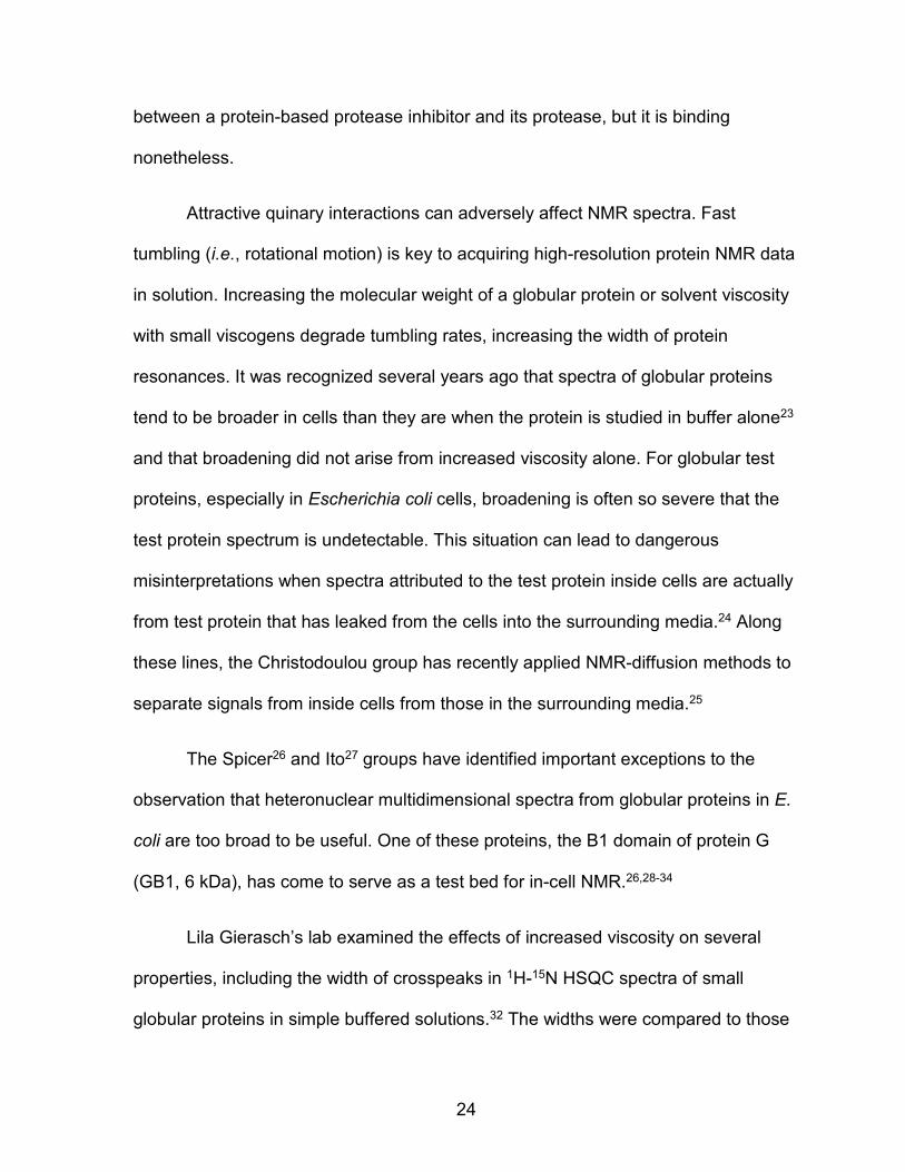
Attractive quinary interactions can adversely affect NMR spectra. Fast

tumbling (i.e., rotational motion) is key to acquiring high-resolution protein NMR data

in solution. Increasing the molecular weight of a globular protein or solvent viscosity

with small viscogens degrade tumbling rates, increasing the width of protein

resonances. It was recognized several years ago that spectra of globular proteins

tend to be broader in cells than they are when the protein is studied in buffer alone23

and that broadening did not arise from increased viscosity alone. For globular test

proteins, especially in Escherichia coli cells, broadening is often so severe that the

test protein spectrum is undetectable. This situation can lead to dangerous

misinterpretations when spectra attributed to the test protein inside cells are actually

from test protein that has leaked from the cells into the surrounding media.24 Along

these lines, the Christodoulou group has recently applied NMR-diffusion methods to

separate signals from inside cells from those in the surrounding media.25

The Spicer26 and Ito27 groups have identified important exceptions to the

observation that heteronuclear multidimensional spectra from globular proteins in E.

coli are too broad to be useful. One of these proteins, the B1 domain of protein G

(GB1, 6 kDa), has come to serve as a test bed for in-cell NMR.26,28-34

Lila Gierasch’s lab examined the effects of increased viscosity on several

properties, including the width of crosspeaks in 1H-15N HSQC spectra of small

globular proteins in simple buffered solutions.32 The widths were compared to those

25

obtained for the same proteins in E. coli cells. The data indicate that the large line

widths in cells cannot be completely explained by a higher viscosity. The authors

concluded that the extra broadening comes from weak transient interactions (i.e.,

quinary interactions) with components of the cytosol.

Peter Crowley’s group obtained direct evidence for these interactions by

examining HSQC spectra of overexpressed cytochrome c (12 kDa) in E. coli lysates

(severe broadening prevented acquisition of in-cell spectra).28 Size exclusion

chromatography as a function of salt concentration in combination with SDS-PAGE

was used to show that the broadening is due to weak interactions. Mutating

positively-charged residues to negatively-charged residues resulted in crosspeak

narrowing and smaller SDS-PAGE-measured molecular weights, indicating that the

quinary contacts involve interactions of positively-charged residues on the

cytochrome with negatively-charged moieties on macromolecules in the lysate. This

important study has placed the focus on charge-charge interactions. Other types of

polar interaction as well as hydrophobic contacts may also play key roles, but

systematic studies have yet to be performed.

Volker Dötsch’s group moved work on quinary interactions into eukaryotic

cells.35 They injected 15N-enriched protein into Xenopus laevis oocytes and again

found that quinary interactions resulted in broad HSQC spectra. Specific

phosphorylation of one of the proteins (the 19 kDa WW domain of peptidyl-prolyl

isomerase Pin1) abrogated the interactions, resulting in observation of the test

protein spectrum in oocytes.

26

Lewis Kay’s group tackled quinary interactions with the test protein

calmodulin (17 kDa) in E. coli lysates. The system provides information about

nonspecific interactions because neither calmodulin nor its specific binding partners

are found in bacteria. The interactions between components of the cytosol and

calmodulin affect protein dynamics on the ps to ns and ms timescales.36 They

measured a lower bound of ~0.2 mM for the binding constant of calmodulin with

cytosolic components (Figure 1.1 a,b).37 These results show that quinary interactions

are strong even in the absence of natural selection. The team also examined what

happens when calmodulin is immersed in yeast lysate. This system has both

biological and physiological relevance because yeast lysate harbors proteins that

specifically bind calmodulin.

The specific interactions

caused further broadening

resulting in complete loss of

the spectrum (Figure 1.1 c).

Figure 1.1. Equilibrium thermodynamic effects of quinary interactions.37 a)

Changes in calmodulin methyl chemical shifts as a function of E. coli lysate concentration indicate nonspecific interactions with lysate constituents on the fast NMR timescale. b) Methyl relaxation data showing the higher viscosity of lysate (100 g/L, orange and green) compared to buffer (red and blue) and the competition between nonspecific biding and specific peptide binding (green and orange). c) HSQC spectra showing that specific binding in Saccharomyces cerevisiae (yeast) lysate replaces nonspecific binding in E. coli lysate resulting in disappearance of the calmodulin spectrum.

As discussed above, some proteins have such strong quinary interactions

that tumbling is too slow for solution NMR. However, lack of rotational motion need

27

not be a barrier; solid state NMR with magic angle spinning is the tool of choice

under these conditions. Reckel et al. used solid-state NMR to examine two

rotationally challenged proteins in E. coli cells.38 Selective 13C- enrichment in

combination with uniform 15N enrichment provided interpretable spectra. Although

solid-state spectra are not yet as informative as solution spectra, solid state NMR of

biological macromolecules is advancing quickly.39

Folding intermediates and crowding

Latham and Kay studied the effects of biologically relevant crowders on protein

folding intermediates.40 They chose an 8 kDa four-helix bundle (the FF domain) as

the test protein and assessed its folding dynamics in E. coli and yeast lysates

(Figure 1.2 a-c). The same intermediate is found in buffer and lysates, but it is more

highly populated in lysates. Further, the exchange rate between native and

intermediate states is slowed. Thus, crowding can affect folding pathways, which

suggests we may not learn all there is to know about physiologically relevant folding

by studying proteins in buffer alone.

We close this section with a warning. A classic approach to understanding the

solvent-protein friction of folding dynamics is to quantify the conversion between

states as a function of viscosity. Using the same four-helix bundle, Sekhar et al.41

showed that a small molecule viscogen (glycerol) and a macromolecular viscogen

(bovine serum albumin) give different results. The discrepancy arises from the sizes

of the viscogens compared to the folding species; only small viscogens yield correct

28

values because, for molecules much smaller than the test protein, the macroscopic

viscosity equals the microscopic viscosity.42

Figure 1.2. Kinetic effects of quinary interactions.40 a) Free energy diagram of the equilibrium between the native state and the intermediate of the FF domain. b) Percent population versus rate plot showing that the intermediate is more highly populated in E. coli lysate and yeast lysate than it is in buffer. c) Plots of shift changes in lysate (upper, E. coli; lower, yeast) showing

that lysates do not affect the structure of the intermediate.

Disordered proteins are different

The interior of a globular protein is similar to that of a billiard ball in that both

are rigid. That is, the parts that comprise the interior of these objects move as a

group. On the other hand, disordered proteins2 are similar to spaghetti in that they

have local, internal motions that are independent of global motion. In cells, the

internal motions are not affected to the same extent as the global motion of globular

proteins. Thus, disordered proteins tend to give higher quality HSQC spectra in cells.

Barnes et al.2 showed this differential effect in a simple experiment by fusing the

disordered protein, α-synuclein (14 kDa), to the small globular protein, ubiquitin (9

kDa). An in-cell HSQC spectrum of the fusion showed only crosspeaks from the

disordered protein. When the cells were lysed and the lysate diluted, loosening

ubiquitin’s quinary interactions, the spectra of both proteins were visible. By

29

examining secondary shifts, Waudby et al. showed that α-synuclein appears to

remain unfolded even in E. coli.5 By monitoring the shift of the protein’s histidine

resonance, these authors also showed that the internal pH of E. coli in dense

slurries acidified to pH 6.2 instead of 7.6. (For further information see Chapter 3.)

Majumber et al. exploited the differential dynamic effect on globular and

disordered proteins to probe binding.43 First, they induced expression of a

disordered protein in 15N-containing media and obtained the expected in-cell

spectrum. Next, they induced expression of its unenriched globular partner. Binding

of the two proteins hindered the local motion of the previously disordered protein,

broadening its resonances into the background. Application of principle component

analysis even allowed the authors to define the binding site on the disordered

partner.

Minimizing effects of attractive quinary interactions on spectra

Methods for obtaining high-resolution spectra of globular proteins in cells are

desirable because attractive quinary interactions broaden resonances. We discuss

two approaches: 19F incorporation and optimization of conventional multidimensional

experiments.

19F is a wonderful in-cell NMR nucleus for eight reasons. First, fluorine is rare

in biological systems,44 which eliminates background. Second, it is 100% abundant.

Third, the NMR sensitivity of 19F is 83% that of 1H, making it one of the most

sensitive nuclei. Fourth, its chemical shift range is large. Fifth, as a spin-1/2 nucleus,

its relaxation properties are similar to those of the proton. Sixth, cells can be coaxed

30

into incorporating aromatic fluorine-labeled amino acids.29 Seventh, replacing a few

hydrogen atoms with fluorine atoms has a minimal effect on structure and stability.45

The eighth advantage is subtle. It might be considered a disadvantage that

only a few fluorine-labeled amino acids are incorporated. However, this situation is

advantageous for studying globular proteins in cells. Simply put, it is easier to

observe a few broad resonances in a one-dimensional spectrum of an 19F-labeled

proteins than it is to observe tens to hundreds of closely packed broad crosspeaks in

a typical multidimensional spectrum of protein uniformly enriched with 15N or 13C.31

Not only can ‘less mean more’ with 19F, the Crowley lab has shown how to make 19F

labeling of tryptophan residues in E. coli an inexpensive endeavor.29 They showed 5-

fluorindole and 6–fluoroindole are incorporated into GB1. The method represents a

15-fold savings compared to the usual scheme for labeling aromatic residues, which

involves, for tryptophan labeling, growth of cells in minimal media containing labeled

tryptophan, an inhibitor of aromatic amino acid synthesis (glyphosate, i.e.,

Roundup™) and unlabeled phenylalanine and tyrosine.46

In one of the first studies to demonstrate the effect of attractive interactions in

cells, Schlesinger et al.47 exploited 19F labeling to show that crowding is not always

stabilizing, because, as explained in the next section, attractive quinary interactions

can overcome crowding-induced short-range repulsions. Ye et al. went on to use 19F

to show that the viscosity in cells is only two-to-three times that in buffer alone, but

quinary interactions make the protein appear much larger than it is. Their work also

emphasizes the fact that care is required in interpreting NMR-relaxation derived in-

cell viscosity measurements, because both quinary interactions and viscosity affect

31

relaxation.

Despite the favorable aspects of 19F labeling, enrichment with 15N and 13C

can yield more detailed information about structure and dynamics. One way to

overcome the broadening-induced overlap is to use selective enrichment.36,37

Latham and Kay showed that incorporating 13C and 2H methyl-enriched Ile, Leu, Val,

or Met gave interpretable 13C–1H correlation spectra in E. coli and yeast lysates.36,37

There are, however, many combinations of enrichment schemes and NMR

experiments. To define a strategy for optimizing in-cell NMR in E. coli, Xu et al.

explored the in-cell NMR of four highly-expressed small (i.e., <20 kDa) globular

proteins in combination with several enrichment methods, including uniform 15N

enrichment with and without deuteration, selective 15N-leucine enrichment, 13C

methyl enrichment of isoleucine, leucine, valine, and alanine (ILVA), fractional 13C

enrichment, and 19F labeling.33 19F labeling gave acceptable results in all instances,

as did 13C ILVA labeling with one-dimensional 13C direct detection in a cryogenic

probe. ILVA enrichment, however, is expensive and such simple spectra might yield

little insight relative to their cost. Xu et al. suggest that uniform 15N enrichment and

19F labeling, both of which are low cost, be tried first. If enrichment yields high quality

HSQC spectra, other approaches will probably work. If an HSQC spectrum of the

protein in cells is not observed, but reasonable 19F spectra are, ILVA enrichment is

worth trying. If both experiments fail, one might try weakening protein-cytoplasm

interactions by exploring charge-change variants.28

32

Quinary interactions and globular protein stability

The effects of crowding on protein stability arise from two phenomena: short

range (steric) repulsions and longer-range interactions. Repulsions stabilize globular

proteins for the simple reason that the crowders take up space, favoring the compact

native state over the expanded denatured state. Longer-range interactions (also

called soft- or chemical- interactions) include hydrogen bonding and charge-charge

interactions. Charge-charge interactions can be stabilizing or destabilizing. Charge-

charge repulsions are stabilizing because they require the crowders to stand off from

the test protein making them occupy even more space. Attractive interactions

between the test protein surface and the crowders, on the other hand, are

destabilizing because unfolding of the test protein exposes more interacting surface.

NMR-detected amide proton exchange is a tool for quantifying the free energy

required to expose backbone amide protons to solvent.48 The largest opening free

energies reflect global protein stability, i.e., the free energy of denaturation. Although

the method provides opening free energies at the residue level, we focus on the

global free energy of opening because interpretation of smaller opening free

energies remains controversial.49,50 Importantly, exchange experiments provide this

information without the addition of heat or denaturing co-solutes, which is important

for systems containing protein crowders because it means crowder stability is

unaffected by the experiment. Several controls are required to ensure that the rate

data yield equilibrium thermodynamic data.51

33

Work in the Pielak lab has been conducted with the small globular proteins,

chymotrypsin inhibitor 2 (CI2, 6 kDa) and GB1. One of the control experiments

mentioned above is to demonstrate that the crowding agent does not affect the

intrinsic rate of exchange in a disordered peptide. This assumption is true for a

number of crowders, including the E. coli cytoplasm (See Chapters 2 and 3).52-54

Synthetic crowders such as Ficoll and polyvinylpyrrolidone have minimal

attractive interactions with CI2. Thus, these crowders stabilize CI2 and other test

proteins.42,53,55,56 CI2, however, is destabilized by protein crowders and the

constituents of E. coli lysate.57 The destabilization suggests the presence of

attractive crowder-test protein interactions, which is consistent with other NMR

experiments on CI2.42 Inomata et al.58 have observed an increase in amide-proton

exchange rates for the test protein ubiquitin in human cells, a result that is also

consistent with the presence of attractive quinary interactions.

Sarkar et al. hypothesized that the interactions involve charge-charge

contacts.59 To test this idea, they refined the lysate by removing the anionic nucleic

acids and negatively charged proteins; CI2 was still destabilized. The result indicates

there remains much to be learned about longer-range interactions and crowding.

Sarkar and Pielak have also shown that the osmolyte glycine betaine can mitigate

the lysate’s destabilizing effect on CI2.60

Monteith et al.61 used amide proton exchange to measure the stability of GB1

in living E. coli cells (Figure 1.3). There are two reasons one might think this would

be an easy experiment. First, GB1 is one of the few globular proteins whose 1H-15N

34

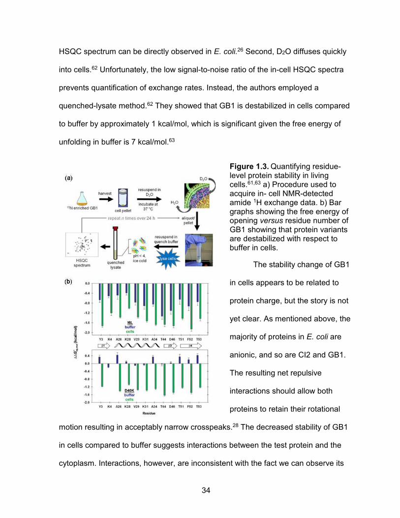
HSQC spectrum can be directly observed in E. coli.26 Second, D2O diffuses quickly

into cells.62 Unfortunately, the low signal-to-noise ratio of the in-cell HSQC spectra

prevents quantification of exchange rates. Instead, the authors employed a

quenched-lysate method.62 They showed that GB1 is destabilized in cells compared

to buffer by approximately 1 kcal/mol, which is significant given the free energy of

unfolding in buffer is 7 kcal/mol.63

Figure 1.3. Quantifying residue-level protein stability in living cells.61,63 a) Procedure used to acquire in- cell NMR-detected amide 1H exchange data. b) Bar graphs showing the free energy of opening versus residue number of GB1 showing that protein variants are destabilized with respect to buffer in cells.

The stability change of GB1

in cells appears to be related to

protein charge, but the story is not

yet clear. As mentioned above, the

majority of proteins in E. coli are

anionic, and so are CI2 and GB1.

The resulting net repulsive

interactions should allow both

proteins to retain their rotational

motion resulting in acceptably narrow crosspeaks.28 The decreased stability of GB1

in cells compared to buffer suggests interactions between the test protein and the

cytoplasm. Interactions, however, are inconsistent with the fact we can observe its

35

HSQC spectrum in cells.28,31-33 CI2 and GB1, show similar responses to the cytosol.

CI2 is negatively charged, its 15H-1H HSQC spectrum cannot be observed in E. coli24

and the protein is destabilized by reconstituted cytosol.57,59 This response of similarly

charged proteins to the cytosol, in addition to the research presented in Chapter 4,

show that anionic proteins are destabilized in cells. However, we still have a great

deal to learn about the nature of these quinary interactions.

NMR in eukaryotic cells

Eukaryotic cells are at the cutting edge of in-cell NMR. Although E. coli is a

good test bed because it is easy to grow and can be coaxed into expressing the

large amounts of test protein required for NMR, the more complex features of

eukaryotic cells make them an important subject for in-cell NMR.

Insect cells and the yeast Pichia pastoris are commonly used to express large

quantities of eukaryotic proteins. Bertrand et al. tested this yeast as a subject for in-

cell NMR using ubiquitin as the test protein.64 Their results are especially informative

about what can happen when proteins are highly expressed. The authors compared

1H-15N HSQC spectra after expression from a methanol inducible promoter under

two conditions. Methanol as the carbon source gave high expression and usable

spectra. A combination of methanol and glucose gave even higher expression, but

the ubiquitin was trapped in expression vesicles, making it essentially a solid. The

resulting diminution of rotational motion broadened its resonances into the

background. Hamatsu et al. have shown that insect cells are also amenable to in-cell

protein NMR with a baculovirus expression system, reporting both15N-1H HSQC

36

spectra and three dimensional spectra of four small globular proteins, including GB1

and calmodulin.30 Thus, these eukaryotes should prove useful for in-cell NMR,

especially for studies of eukaryotic-specific post-translational modifications.

Higher eukaryotic cells are fussier than E. coli. For instance, E. coli can be

examined under anaerobic conditions, but most higher-eukaryotic cells are sensitive

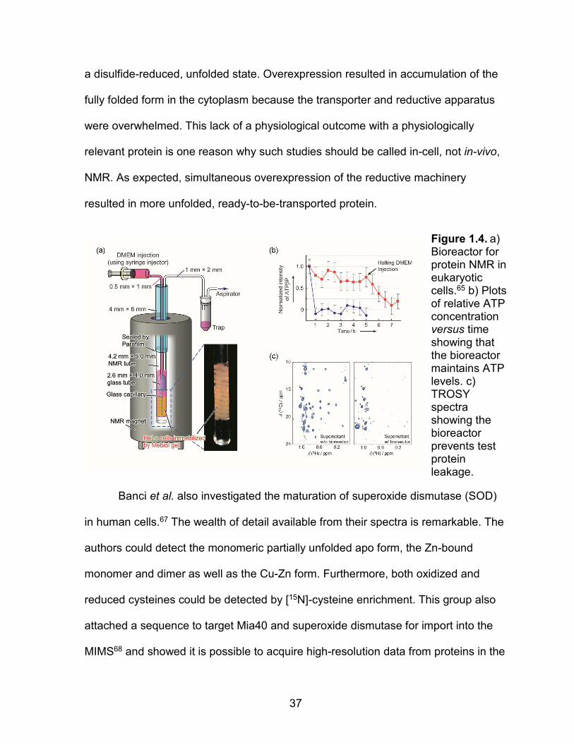
to nutrient depletion and require oxygenation. Kubo et al. developed a clever

bioreactor that solves these problems.65 Cells are fixed in a gel in the sensitive part

of the probe where they can be easily perfused with fresh oxygenated media (Figure

1.4). The authors tested the bioreactor by using 31P NMR to examine ATP levels.

Without the bioreactor, ATP depletion was complete in 30 min. With the bioreactor,

cells maintained their ATP levels for the duration of the experiment (5 h). They also

investigated the in-cell 1H-13C HMQC spectra of a 9- kDa methyl ILV 13C-enriched

microtubule binding protein. The protein was introduced into the cells via a pore-

forming toxin. Transferred cross saturation experiments and competition

experiments with unenriched protein helped define the binding site and showed

specific microtubule binding. Importantly, the binding site in cells is similar to that

discovered in vitro. These experiments also illuminate an important point about

protein leakage. In the absence of the bioreactor only 10-20% of the protein leaked,

but almost all the signal arose from the leaked protein because the quinary

interactions in cells led to severe broadening.

The Banci group has characterized the maturation of the mitochondrial

intermembrane space (MIMS) protein, Mia40 (16 kDa) in human cells.66 To reach

their destination, MIMS proteins must be transported through the outer membrane in

37

a disulfide-reduced, unfolded state. Overexpression resulted in accumulation of the

fully folded form in the cytoplasm because the transporter and reductive apparatus

were overwhelmed. This lack of a physiological outcome with a physiologically

relevant protein is one reason why such studies should be called in-cell, not in-vivo,

NMR. As expected, simultaneous overexpression of the reductive machinery

resulted in more unfolded, ready-to-be-transported protein.

Figure 1.4. a) Bioreactor for protein NMR in eukaryotic cells.65 b) Plots of relative ATP concentration versus time showing that the bioreactor maintains ATP levels. c) TROSY spectra showing the bioreactor prevents test protein leakage.

Banci et al. also investigated the maturation of superoxide dismutase (SOD)

in human cells.67 The wealth of detail available from their spectra is remarkable. The

authors could detect the monomeric partially unfolded apo form, the Zn-bound

monomer and dimer as well as the Cu-Zn form. Furthermore, both oxidized and

reduced cysteines could be detected by [15N]-cysteine enrichment. This group also

attached a sequence to target Mia40 and superoxide dismutase for import into the

MIMS68 and showed it is possible to acquire high-resolution data from proteins in the

38

inter-membrane space of intact mitochondria.

Continuing with SOD, Danielsson et al. took a different approach.69 Instead of

expressing the protein in human cells, they expressed and purified the isotopically-

enriched protein from E. coli and covalently attached a cell penetrating peptide to an

engineered cysteine on SOD. Initial attempts to introduce sufficient amounts into

HeLa cells were unsuccessful. Success came after increasing the positive charge on

SOD. The success of the charge changes makes sense considering our knowledge

of cell penetrating proteins: they must overcome the negative charge on the test

protein to which they are attached. Another key point involving a pre-enriched

protein65 is that the NMR-active nuclei are less likely to find their way into

metabolites and other proteins that obscure the test-protein spectrum.

We close this section by comparing the quality of in-cell spectra from bacterial

and eukaryotic cells. With rare exceptions,26,27 multidimensional spectra from

globular protein are difficult to observe in E. coli. As discussed above, the situation is

better in eukaryotic cells. It is not entirely clear why this should be the case, but one

clue may be the lower concentration of protein plus nucleic acid in eukaryotic cells

(100-300 g/L) compared to E. coli cells (300-500 g/L).2 It is important to bear in

mind, however, that eukaryotic cells are far from a panacea because not all proteins

that should be observable by in-cell NMR in eukaryotes are observed.66 The

difference between what should happen and what does happen extends to methods

for getting isotopically enriched proteins into higher eukaryotic cells. Besides

injection, which is only reasonable for oocytes, the most common methods are

attachment of a cell-penetrating peptide, use of a toxin to open pores in the

39

membrane and electroporation.70 It is unclear, however, which method will work best

in any particular combination of test protein and cell.

Summary and closing thoughts

NMR has taken the lead in adding to our understanding of how quinary

structure affects protein stability, folding pathways, ligand binding and side chain

dynamics. Selective labeling strategies have been shown to be useful when these

interactions broaden protein resonances into the baseline. In addition, sophisticated

NMR strategies are being applied to not only E. coli proteins, but also to several

types of eukaryotic cells. Nevertheless, the field remains in its infancy. We are

picking the low hanging fruit: typical test proteins have molecular weights of

approximately 10 kDa, but the average molecular weight an E. coli protein is 30 kDa.

The average eukaryotic protein is even larger.71 In addition, we need models to

explain how proteins of similar size, shape and surface properties interact differently

with the cytosol. Therefore, the most important and challenging frontier is the study

of larger test proteins, because crowding effects are predicted to scale with

molecular weight.72

40

CHAPTER 2: AMIDE PROTON EXCHANGE OF A DYNAMIC LOOP IN CELL EXTRACTS

Edited from: Smith AE, Sarkar M, Young GB, Pielak GJ. Protein Science. 22,1313-

1319 (2013)

Abstract

Intrinsic rates of exchange are essential parameters for obtaining protein

stabilities from amide 1H exchange data. To understand the influence of the

intracellular environment on stability, one must know the effect of the cytoplasm on

these rates. We probed exchange rates in buffer and in Escherichia coli lysates for

the dynamic loop in the small globular protein chymotrypsin inhibitor 2 using a

modified form of the solvent exchange NMR experiment, SOLEXSY. No significant

changes were observed, even in 100 g dry weight L-1 lysate. Our results suggest

that intrinsic rates from studies conducted in buffers are applicable to studies

conducted under cellular conditions.

41

Introduction

The cytoplasm of Escherichia coli is a milieu of macromolecules whose total

concentration can exceed 300 gL-1.1,73 This crowded environment is expected to

affect biophysical properties, such as protein stability.74 Quantifying these changes is

key to understanding protein chemistry in cells.75

1H/2H exchange has been used to assess protein stability since Linderstrøm-

Lang and colleagues laid the theoretical framework in the 1950s.76-78 Native globular

proteins exist in equilibrium with a large ensemble of less structured states.48 When

a protein in H2O is transferred to 2H2O, solvent-exposed amide protons in the native

state can, in most cases,79 exchange freely with deuterons. Hydrogen-bonded and

other protected protons, however, exchange only upon exposure to solvent during a

transient opening (equation 1),

where Kop=kop/kcl is the opening equilibrium constant, kop and kcl are the opening

and closing rate constants, respectively, and kint is the intrinsic rate of amide 1H

exchange in an unstructured peptide. When intrinsic exchange is rate limiting (kcl >

kint), the observed exchange rate of a protonated amide (kobs) can be used to

determine the modified standard free energy of opening (i.e., the stability), because

kobs = Kopkint (equation 2).51,78,80

ΔGop°' = -RTlnKop = -RTln

kobs

kint

(2)

42

This approach is valid for protons that are exposed on global unfolding, so called

“globally exchanging residues,” because maximum values of ΔGop°' often equal the

free energy of denaturation measured by using independent techniques.78,81,82

To validate the 1H/2H exchange results, one must know if kint changes under

crowded conditions. kint values in buffer can be calculated as a function of primary

structure, pH, and temperature83-85 using the online resource, SPHERE.86 These

values have also been used to measure protein stability in solutions crowded by

synthetic polymers and proteins, because as described below, these crowding

agents do not affect kint.53,87-89 Saturation transfer NMR was used to show that the

kint of poly-DL-alanine does not change in 300 gL-1 70 kDa of Ficoll or its monomer,

sucrose.53,90 Information about crowding induced changes in intrinsic rates can also

be gleaned from dynamic loops of globular proteins.

Chymotrypsin inhibitor 2 (CI2; Figure 2.1A) is a globular protein91 (Figure

2.1A) that has been extensively studied by amide 1H/2H exchange.82,87,92,93 Residues

in its reactive loop are potential models for assessing kint, because they possess few

hydrogen bonds, lower than average order parameters,94 high B-factors,91 and large

solvent accessible surface areas (SASAs; Figure 2.1B). Phase-modulated CLEAN

chemical exchange (CLEANEX) experiments95 conducted in buffer and under

crowded conditions show that exchange rates in the loop do not change in solutions

containing 300 gL-1 40-kDa poly-vinyl-pyrrolidone (PVP),87 100 gL-1 lysozyme and

100 gL-1 bovine serum albumin.88 These observations suggest that kint values in

buffer can be applied to experiments conducted with these crowding agents.

43

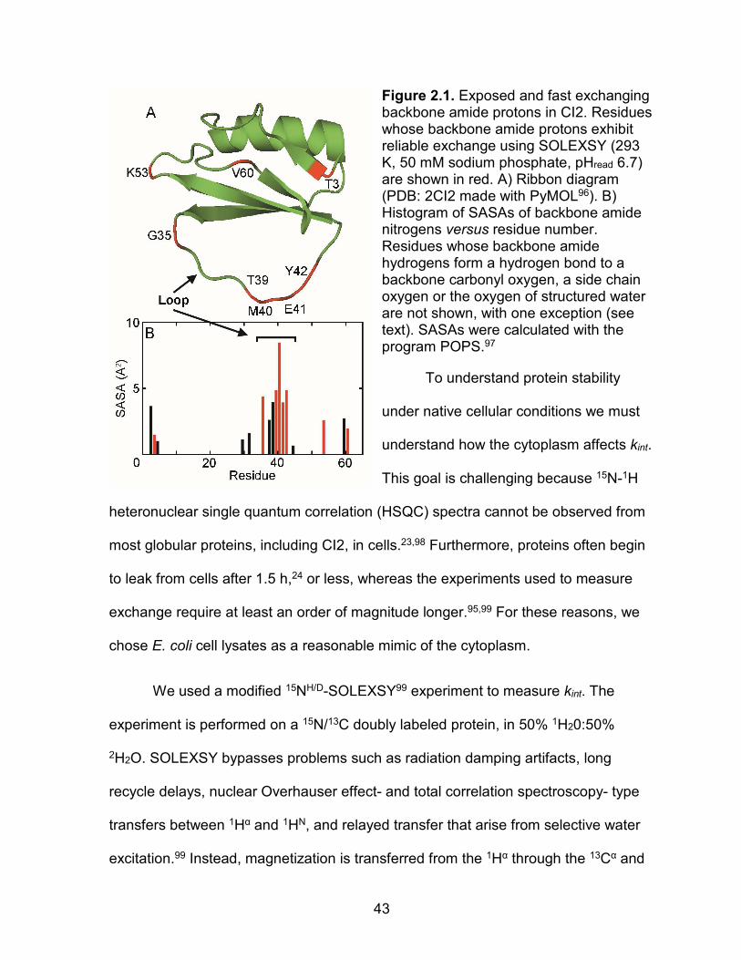
Figure 2.1. Exposed and fast exchanging backbone amide protons in CI2. Residues whose backbone amide protons exhibit reliable exchange using SOLEXSY (293 K, 50 mM sodium phosphate, pHread 6.7) are shown in red. A) Ribbon diagram (PDB: 2CI2 made with PyMOL96). B) Histogram of SASAs of backbone amide nitrogens versus residue number. Residues whose backbone amide hydrogens form a hydrogen bond to a backbone carbonyl oxygen, a side chain oxygen or the oxygen of structured water are not shown, with one exception (see text). SASAs were calculated with the program POPS.97

To understand protein stability

under native cellular conditions we must

understand how the cytoplasm affects kint.

This goal is challenging because 15N-1H

heteronuclear single quantum correlation (HSQC) spectra cannot be observed from

most globular proteins, including CI2, in cells.23,98 Furthermore, proteins often begin

to leak from cells after 1.5 h,24 or less, whereas the experiments used to measure

exchange require at least an order of magnitude longer.95,99 For these reasons, we

chose E. coli cell lysates as a reasonable mimic of the cytoplasm.

We used a modified 15NH/D-SOLEXSY99 experiment to measure kint. The

experiment is performed on a 15N/13C doubly labeled protein, in 50% 1H20:50%

2H2O. SOLEXSY bypasses problems such as radiation damping artifacts, long

recycle delays, nuclear Overhauser effect- and total correlation spectroscopy- type

transfers between 1Hα and 1HN, and relayed transfer that arise from selective water

excitation.99 Instead, magnetization is transferred from the 1Hα through the 13Cα and

44

carbonyl carbon to the amide 15N. The 15N chemical shift is then encoded to produce

two signals, 15ND and 15NH.

After encoding, a variable mixing time monitors the exchange of 15ND and

15NH for each hydrogen isotope, and magnetization is transferred to 1H for detection.

At short mixing times, only protonated species are observed, because only

protonated amide nitrogens are detected at the 1H frequency (Figure 2.2). The

chemical shift of 15ND is also recorded, but at short mixing times no signal is

detected because little 1H has exchanged onto the deuterated amide. At longer

times, exchange of 1H onto the initially deuterated (15ND) site causes an increase in

the volume of the 15ND/1H crosspeak, producing a buildup curve (Figure 2.2B). The

exchange of deuterons onto the initially protonated site causes a decrease in

volume, and a corresponding decay with time (Figure 2.2B). Plots of peak volume

versus time can be fitted to yield kint. High quality data can be obtained for rates of

between 0.3 and 5.0 s-1.99

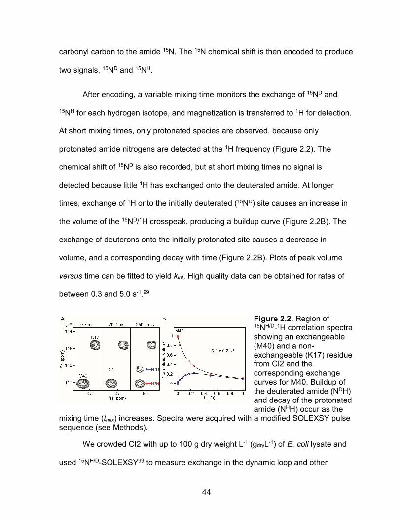
Figure 2.2. Region of 15NH/D-1H correlation spectra showing an exchangeable (M40) and a non-exchangeable (K17) residue from CI2 and the corresponding exchange curves for M40. Buildup of the deuterated amide (NDH) and decay of the protonated amide (NHH) occur as the

mixing time (tmix) increases. Spectra were acquired with a modified SOLEXSY pulse sequence (see Methods).

We crowded CI2 with up to 100 g dry weight L-1 (gdryL-1) of E. coli lysate and

used 15NH/D-SOLEXSY99 to measure exchange in the dynamic loop and other

45

exposed regions. Exchange rates are largely unchanged in lysates compared to

buffer alone. Our results suggest that kint values from buffer based experiments (i.e.,

from SPHERE) are valid for quantifying protein stability under cellular conditions.

Results

Lysate solutions are problematic for two reasons. First, at high concentrations

they are not stable enough to allow acquisition of a full 60-h SOLEXSY experiment

(Figure 2.3). Second, weak interactions between constituents of the lysate and the

protein being studied result in a shorter transverse relaxation time (T2), leading to

broad resonances that degrade the quality of the spectra used to create buildup and

decay curves.42,98,100

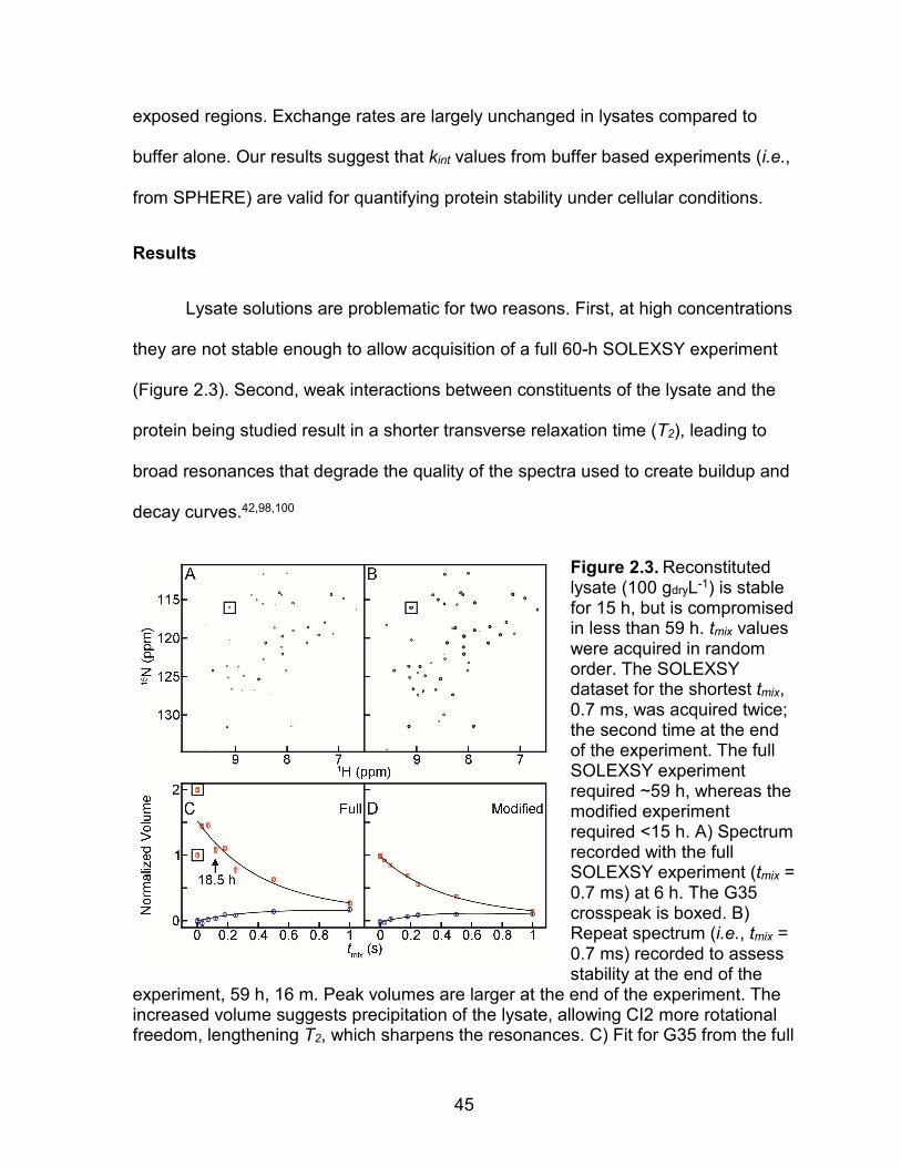
Figure 2.3. Reconstituted lysate (100 gdryL-1) is stable for 15 h, but is compromised in less than 59 h. tmix values were acquired in random order. The SOLEXSY dataset for the shortest tmix, 0.7 ms, was acquired twice; the second time at the end of the experiment. The full SOLEXSY experiment required ~59 h, whereas the modified experiment required <15 h. A) Spectrum recorded with the full SOLEXSY experiment (tmix = 0.7 ms) at 6 h. The G35 crosspeak is boxed. B) Repeat spectrum (i.e., tmix = 0.7 ms) recorded to assess stability at the end of the

experiment, 59 h, 16 m. Peak volumes are larger at the end of the experiment. The increased volume suggests precipitation of the lysate, allowing CI2 more rotational freedom, lengthening T2, which sharpens the resonances. C) Fit for G35 from the full

46

SOLEXSY experiment, which required 59 h. Instead of decaying, the volume of the 120 ms point (vertical arrow, acquired at ~19 h) is greater than that for the 0.7 ms point, acquired at 6 h, indicating breakdown of the lysate. Consistent with this idea, precipitate was visible at ~60 h. D) G35 data acquired with the modified experiment, which required only ~15 h. The repeated tmix point, acquired at 14 h, is on top of the point acquired at 1 h, suggesting that the lysate was stable over the course of the modified experiment. Consistent with this idea, no precipitate was observed at the end of the experiment.

In an attempt to overcome the stability problem, we decreased the acquisition

time by reducing the number of scans, but this approach exasperated the

broadening problem. We then tried removing the sign-coding portion of the

SOLEXSY experiment. In combination with acquiring fewer t1 points, this change

enabled us to acquire a complete experiment in 15 h. Furthermore, the consequent

removal of 10.6 ms (~1

JNH) from the pulse sequence resulted in a mean increase in

signal to noise ratio of 25% in buffer (depending on the resonance, Supplementary

Figure 2.1A), which helped compensate for the decreased sensitivity arising from the

shorter T2 values in lysate (Supplementary Figure 2.1B). The original and modified

SOLEXSY experiments were validated by comparing rates acquired in buffer to

mathematical predictions and to values obtained with CLEANEX79,88 (Supplementary

Table 2.1).

Residues useful for assessing kint values should lack stable hydrogen bonds.

Backbone amide hydrogens from 15 residues of CI2 do not form hydrogen bonds to

a backbone carbonyl oxygen, a side chain oxygen or the oxygen of structured

water.91 These residues are in loops, and as expected, exhibit significant SASAs

(Figure 2.1B). We also included E41, whose backbone amide 1H is within hydrogen

47

bonding distance (2.6 Å for the heavy atoms) of the carbonyl oxygen of T39, in our

analysis because loop motion likely makes any hydrogen bond transient.

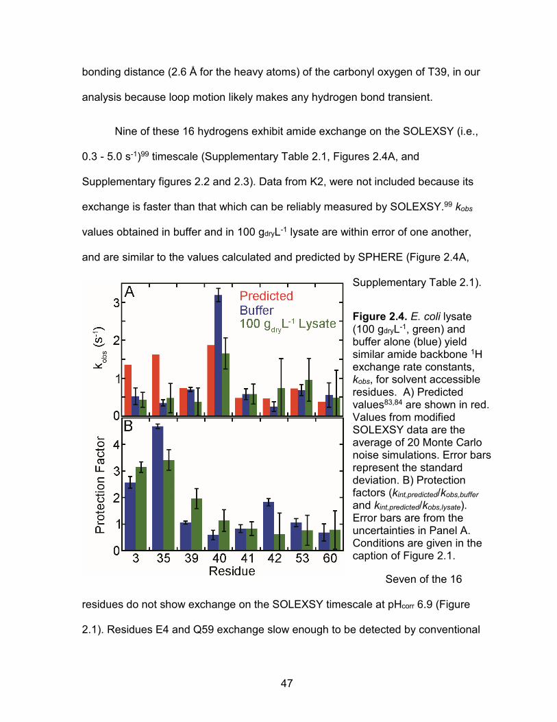
Nine of these 16 hydrogens exhibit amide exchange on the SOLEXSY (i.e.,

0.3 - 5.0 s-1)99 timescale (Supplementary Table 2.1, Figures 2.4A, and

Supplementary figures 2.2 and 2.3). Data from K2, were not included because its

exchange is faster than that which can be reliably measured by SOLEXSY.99 kobs

values obtained in buffer and in 100 gdryL-1 lysate are within error of one another,

and are similar to the values calculated and predicted by SPHERE (Figure 2.4A,

Supplementary Table 2.1).

Figure 2.4. E. coli lysate (100 gdryL-1, green) and buffer alone (blue) yield similar amide backbone 1H exchange rate constants, kobs, for solvent accessible residues. A) Predicted values83,84 are shown in red. Values from modified SOLEXSY data are the average of 20 Monte Carlo noise simulations. Error bars represent the standard deviation. B) Protection factors (kint,predicted/kobs,buffer and kint,predicted/kobs,lysate). Error bars are from the uncertainties in Panel A. Conditions are given in the caption of Figure 2.1.

Seven of the 16

residues do not show exchange on the SOLEXSY timescale at pHcorr 6.9 (Figure

2.1). Residues E4 and Q59 exchange slow enough to be detected by conventional

48

1H2O-to-2H2O transfer experiments.53,82 The other five residues (A29, V31, H37, V38,

I44) show chemical exchange using CLEANEX, but these data were acquired at

higher pH.79 Extrapolating these data to our conditions (pOH = 7.71)101 and using an

Arrhenius activation energy (Ea)83of 17 kcalmol-1, leads to kint values between 0.001

s-1 and 0.04 s-1, which are too small to be accurately assessed with SOLEXSY.

Discussion

Knowing how the cytoplasm affects 1H/2H amide exchange of exposed

residues is vital to calculating opening free energies and global stabilities.51,53,87

Although these values are normally obtained from SPHERE, the server only predicts

values in solutions made with 100% 1H2O or 2H2O. The SOLEXSY experiment,

however, is conducted in a 1:1 2H2O:1H2O mixture. To obtain a direct comparison to

our solution conditions we calculated the rates using the equations that drive

SPHERE, but with different parameters. Rates were calculated stipulating a buffer

made from 1:1 2H2O:1H2O (pHcorr 6.9, pKW 14.61), with poly-DL-alanine as the

reference molecule and kb,ref for ND exchanging in 1H2O.83-85,101 These rates were

then halved99 to make them comparable to those from experiment and SPHERE.

This manipulation accounts for the fact that exchange onto 15ND is only visible by

SOLEXSY when 1H exchanges. In other words, 2H exchange onto initially

deuterated amides is undetected, because only 1H is visible at the 1H frequency,

making the predicted rate twice that measured by SOLEXSY. These corrected

values closely match those obtained from SPHERE by using the poly-DL-alanine

rate basis, with a pHread 6.5, in 100% 2H2O (Supplementary Table 2.1).

49

The corrected rates are also similar to rates measured in buffer (Figure 2.4A)

and obtained with CLEANEX (Supplementary Table 2.1).79,88 Slight deviations from

the CLEANEX results are likely due to differences in solvent condition; the

SOLEXSY experiments used 1:1 2H2O:1H2O and a different ionic strength. Taken

together these results suggest that SOLEXSY is a useful experiment for measuring

exchange rates in disordered loops of globular proteins.

The rates are also similar to those measured in lysate (Figure 2.4), indicating

that lysate at 100 gdryL-1 has an insignificant effect on exchange. Protection factors

(kint/kobs) of less than five are an unreliable indicator of secondary structure,102

whereas residues that exchange only on complete unfolding (i.e., globally

exchanging residues) can have protection factors greater than 105.53,55,82,87,93

Protection factors based on the SOLEXSY data (kint,predicted/kobs,buffer and

kint,predicted/kobs,lysate), are no larger than five for the loop region (Figure 2.4), and even

these may reflect small errors in the parameters used to drive SPHERE. Taken

together, the data indicate that small differences in kobs values between lysate and

buffer will have small effects on protein stability studies conducted in lysates.

The concentration of macromolecules in the cytoplasm of E. coli is 300 gL-1,

or even higher.1,73 Our attempts to acquire SOLEXSY data at these concentrations

were unsuccessful for the reasons discussed above: chemical instability of the lysate

and interaction-induced resonance broadening. Nevertheless, rates obtained in 0,

25, 50 and 100 gdryL-1 lysate show no general and consistent trend (Figures 2.5 and

Supplementary Figure 2.4), suggesting our results are applicable to the dense

interior of the bacterial cell.

50

Figure 2.5. Comparison of 0 - 100 gdryL-1 lysate show no general and consistent trend. A) Values from SOLEXSY data are the average of 20 Monte Carlo noise simulations. Error bars represent the standard deviation. Data were acquired with the modified SOLEXSY experiment for buffer and 100 gdryL-1 lysate. The full experiment was used for 25 and 50 gdryL-1 lysate. B) Protection factors (kint,predicted/kobs,SOLEXSY). Predicted values were calculated as described in the footnote to Table S1. Error bars are the same as in Panel A. Protection factors of less than 5 are not a reliable predictor of structure.102

Methods

Protein. 13C glucose (2.0 gL-1) and 15NH4Cl (1.0 gL-1) were used to produce

purified CI2.42,87 Purity was assessed by SDS-PAGE.

Lysate. Lysates were obtained by modifying the method described by Wang

et al.42 Competent BL21-DE3 (Gold) E. coli were transformed with the pET28a

vector harboring the kanamycin resistance gene. The transformants were plated on

Luria-Bertani (LB) agar plates containing 60 µg/ml kanamycin. The plates were

incubated overnight at 37 oC. A single colony was added to 60 mL of LB liquid media

containing 60 µg/ml kanamycin. The culture was shaken overnight (New Brunswick

Scientific, Innova, I26) at 225 rpm and 37 oC, then equally divided into four, 2.8 L

baffled flasks, each containing 1 L of LB and 60 µg/ml kanamycin. This culture was

51

grown to saturation (9 h). The cells were pelleted at 6500 g for 30 min and the

pellets stored at -20 oC.

Each frozen cell pellet was thawed, resuspended and lysed in 25 mL of 25

mM Tris-HCl (pH 7.6) containing a cocktail of protease inhibitors [Sigma-Aldrich:

0.02 mM 4-(2-aminoethyl) benzenesulfonyl fluoride, 0.14µM E-64, 1.30 µM bestatin,

0.01 µM leupeptin, 3.0 nM aprotinin and 0.01 mM sodium EDTA, 0.01 mM, final

concentrations]. Lysis was accomplished by sonic dismembration on ice for 6 min

(Fischer Scientific, Sonic Dismembrator Model 500, 20% amplitude, 2 s on, 2 s off).

After lysis, cell debris was removed by centrifugation (14000 g at 10 oC for 40 min).

The supernatant was filtered through a 0.22 µm Durapore® PVDF membrane

(Millipore).

The filtrates were pooled (~ 37 mL per L culture) and dialyzed (Thermo

Scientific, SnakeSkin, 3K MWCO) at 4 oC against 5 L of 10 mM Tris-HCl, 0.1% NaN3

(pH 7.6) for 72 h. The buffer was changed every 24 h. The inhibitor cocktail was

added to each dialysate. After lyophilization (Labconco, Freezone Plus 2.5), the

straw-colored powder was stored at -20 oC. To ensure that the lysate contained 50%

exchangeable protons and 50% exchangeable deuterons, the powder was

resuspended in 50% D2O (Cambridge Isotopes Laboratories), incubated at room

temperature for 8 h and lyophilized. The process was performed twice and the

resultant powder (300.0 mg) was resuspended in sufficient 50% deuterated sodium

phosphate buffer (50 mM, pHread 6.7) to give 3.0 mL of solution with a final

concentration of 1.0 x 102 gdry weight L-1. The pHread was adjusted to 6.7. The solution

was centrifuged at 14000 g for 10 min. The supernatant contained 52 ± 4 gL-1 of

52

protein as determined by a modified Lowry assay sing bovine serum albumin as the

standard (Thermo Scientific). The uncertainty in the concentration is the standard

deviation of the mean from triplicate measurements.

NMR. 13C, 15N enriched CI2 was added to sodium phosphate buffer (50 mM,

50% 1H2O:50% 2H2O, pHread 6.7) with and without lysate. The final CI2

concentration was ~1 mM for samples acquired in buffer alone with the modified

SOLEXSY experiment. A concentration of 1.5 mM was used for all other

experiments. The concentrations in buffer were verified by measuring the

absorbance at 280.0 nm (ε = 7.04 x 103 M-1 cm -1).103

A modified SOLEXSY experiment99 was used to measure exchange rates

(Appendix 1). Sign coding was originally used to facilitate data acquition on

intrinsically disordered proteins by reducing the number of crosspeaks.99 The

spectra of globular proteins like CI2 are well dispersed, elimiating the need for this

feature. We removed the 10.6 ms sign coding period,

� 1

2JNH� -90x

°90±x° � H1 �,180x

° � N15 �-(1

2JNH).

Data were acquired at 293 K on a 600 MHz Bruker Avance III HD

spectrometer equipped with a HCN triple resonance cryoprobe (Bruker TCI) and

Topspin Version 3.2 software. Sweep widths were 9600 Hz in the 1H dimension and

2300 Hz in the 15N dimension. Twenty-four transients were collected using 1024

complex points in t2 with 128 TPPI points in t1 for each mixing time. Data were

collected in a pseudo-3D mode with mixing times of 0.7, 1000.7, 250.7, 120.7, 30.7,

180.7, 70.7, 500.7 ms. An additional spectrum with a 0.7 ms mixing time was

53

collected at the end of the experiment to assess lysate stability. The 120.7 ms data

point was omitted for the 100 gdryL-1 lysate. Acquisition required approximately 15 h

per sample. The full experiment used the same parameters, except that 256 points

in t1 were used for each mixing time, and required ~60 h per sample.

Data processing. Data were processed with NMRPipe.104 The t2 data were

subjected to a 60° shifted squared sine bell function (800 complex points for buffer

alone and 512 complex points for lysate) prior to zero-filling to 8096 points and

Fourier transfomation. The t1 data were linear predicted to 256 points prior to

application of a 60°-shifted squared sine bell. The t1 data were then zero-filled to

2048 points and Fourier-transformed. The spectra were peak picked and integrated

using the built in automated routines. Peak volumes were fitted as described.99

When the full experiment was used similar routines were followed without linear

prediction. Sign encoded spectra were added or subtracted to create buildup and

decay spectra, respectively.

54

Supplementary Information for Chapter 2

Supplementary Table 2.1. Exchange rates (s-1) in buffer.

SOLEXSYc CLEANEX-PM Residue SPHEREa Predictionb Full Modified M et al.d H et al.e

3 1.49 1.35 0.7 ± 0.2 0.5 ± 0.2 NRf 0.3

35 1.79 1.63 0.56 ± 0.04 0.35 ± 0.08 NR 0.5

39 0.82 0.74 0.4 ± 0.2 0.70 ± 0.06 0.5 ± 1 0.2

40 2.05 1.87 2.58 ± 0.04 3.2 ± 0.2 NR 1.8

41 0.53 0.48 0.5 ± 0.1 0.6 ± 0.1 0.5 ± 1 NR

42 0.51 0.46 0.57 ± 0.02 0.3 ± 0.1 0.4 ± 0.2 0.1

53 0.80 0.73 0.67 ± 0.03 0.7 ± 0.1 1 ± 1 0.4

60 0.42 0.38 0.35 ± 0.08 0.6 ± 0.3 NR 0.4

Footnotes

abased on CI2 sequence using the online server SPHERE, poly-DL-alanine rate basis, pH 6.5, 100% D2O83,84,86

bRates were calculated as described99 using the method introduced by Bai, et al.83,85 logkb,ref and logkw,ref are from Connelly, et al.84 pOH was calculated taking into account the 50% H2O:50% D2O solution.101 After calculation, rates were halved, as discussed in the main text.

cfitted as described.99 Averages from Monte Carlo analysis along with their uncertainties. pHcorr 6.9, 50 mM NaPO4,293 K, 50% D2O

dCLEANEX95 data from Miklos, et al.88 pH 6.5, 50 mM NaPO4, 293 K, 10% D2O. Rates halved to account for H2O concentration.

eRelaxation compensated105 CLEANEX95 data from Hernandez, et al.79 pH 7: 20 mM NaPO4, total ionic strength 150 mM, 298 K. To mimic our experimental conditions: pOH (7.71, as calculated)101 was subtracted from logkOH to obtain logkint. These values were then extrapolated to 293 K using the Arrhenius equation and an activation energy of 17 kcal/mol.83 Rates halved to account for H2O concentration.

fNot Reported

55

Supplementary Figure 2.1. Increase in signal from removing the sign-coding portion of the SOLEXSY pulse sequence. Sign-coded spectra are shown in red. Spectra without coding are shown in blue. Spectra are the first increment of the respective SOLEXSY experiments acquired with 24 scans and processed in Topspin using the first 1024 points of the FID, a cosine squared window function and zero-filling to 8192 points. Signal to noise ratios were measured using the built-in .sino module with a noise region of 3 to -1 ppm. A) A mean signal to noise increase of 24% is seen for the 250 ms plane in dilute solution. B) A mean signal to noise increase of 176% is seen in 100 gL-1 lysate for the 0 ms plane.

56

Supplementary Figure 2.2. Buildup and decay curves for N- and C-terminal regions of CI2. Crosspeak volume is plotted against time for NDH (blue circles) and NHH (red squares) resonances, creating buildup and decay curves, respectively. Data for each residue are fitted99 to yield its rate of amide proton exchange. Error bars are the standard deviation of peak volumes in 20 spectra with representative amounts of added noise. The upper value in each panel is the fitted rate along with its uncertainty. The lower value is the average rate from the Monte Carlo analysis along with its uncertainty. The modified SOLEXSY pulse sequence (see Methods) was used.

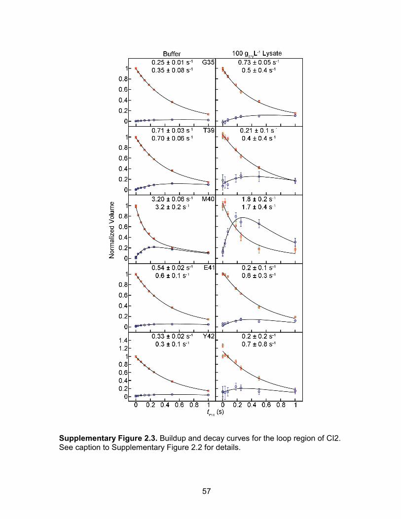
57

Supplementary Figure 2.3. Buildup and decay curves for the loop region of CI2. See caption to Supplementary Figure 2.2 for details.

58

Supplementary Figure 2.4. To ensure the data in Figure 2.4 of were unaffected by our use of the modified experiment for the ‘Buffer’ sample, we reacquired those data using the full sequence (the remainder of the data is copied from Figure 2.4). The change does not affect our conclusions. A) Values from SOLEXSY data are the average of 20 Monte Carlo noise simulations. Error bars represent the standard deviation of the mean. B) Protection factors (kint,predicted/kobs,SOLEXSY). Predicted values were calculated as described in the footnote to Supplementary Table 2.1. Error bars are the same as in Panel A. Protection factors of less than 5 are not a reliable predictor of structure.102

59

CHAPTER 3: HYDROGEN EXCHANGE OF DISORDERED PROTEINS IN ESCHERICHIA COLI

Original citation: Smith AE, Zhou Z, Pielak GJ. Protein Science. 24, 706-713 (2015)

Abstract

A truly disordered protein lacks a stable fold and its backbone amide protons

exchange with solvent at rates predicted from studies of unstructured peptides. We

have measured the exchange rates of two model disordered proteins, FlgM and α-

synuclein, in buffer and in Escherichia coli using the NMR experiment, SOLEXSY.

The rates are similar in buffer and cells and are close to the rates predicted from

data on small, unstructured peptides. This result indicates that true disorder can

persist inside the crowded cellular interior and that weak interactions between

proteins and macromolecules in cells do not necessarily affect intrinsic rates of

exchange.

60

Introduction

Cellular processes occur at macromolecule concentrations of 300-400 g/L.1,73

The resulting weak, nonspecific interactions between macromolecules in the

cytoplasm alter globular protein dynamics and stability.40,57,61,74 Disordered proteins

are fundamentally different. Unlike many model, single domain, globular proteins,

whose structures do not change until they denature,18 the properties of disordered

proteins depend on solution conditions.2 Thus, the crowded nature of the cell could

have large effects on protein disorder. Studies show that the cellular interior can

promote structure formation in proteins that are only transiently structured in

buffer.106 On the other hand, there is a growing realization from studies of globular

proteins that attractive interactions favor less structure.57,88,89,107-110

To date, knowledge of the atomic-level structure of disordered proteins inside

cells comes from a crude measure: the presence or absence of crosspeaks in 15N-

1H HSQC NMR spectra.5,106 Absence of peaks is caused by chemical exchange and

is explained in contrasting ways: 1) intramolecular exchange involving the

stabilization of particular conformations (i.e., folded species) and 2) weak, transient

chemical interactions between the test protein and cellular components.23,28,106,111

Here, we take a new approach by quantifying hydrogen exchange rates for two

proteins possessing different degrees of disorder.

Structure protects backbone amide protons from solvent exchange.48

Therefore, measuring their exchange rates inside cells and comparing the values to

those measured in buffer and calculated from unstructured peptides provides

61

information about structure. Protection is quantified as the rate in an unstructured

peptide (~0.1 - 10 s-1)83 divided by the observed rate, kint/kobs. These protection

factors range from >105 for backbone amide protons in the core of globular proteins

to <5 for denatured proteins.57,61,102 Intrinsic rates in buffer are estimated by using

the online program, SPHERE,86 which calculates kint based on data from

unstructured peptides and information about the system (i.e., primary structure, pH,

deuterium content, and temperature).83,84 These calculated rates remain valid in

buffers containing physiologically relevant concentrations of globular proteins and

cell lysates.52,88

Direct measurement of exchange in cells, however, is challenging. We

investigated the disordered proteins α-synuclein and FlgM, both of which give in-cell

NMR spectra,106,111-113 using the SOLEXSY experiment52,99 to quantify kobs in

Escherichia coli and buffer. SOLEXSY uses a variable mixing time (tmix) to monitor

hydrogen exchange (Supplementary Figure 3.1). Short times do not result in a

buildup crosspeak. Longer times allow amide deuterons to exchange for protons and

buildup of the initially deuterated amide crosspeak occurs. Likewise, a decay is

observed from the initially protonated species. Rates are obtained from fits of peak

volume versus mixing time.

α-Synuclein is a 140-residue protein found at the presynaptic terminals of

neurons.114 Its exact role is controversial, but the protein is N-terminally acetylated

and thought to play a part in dopamine trafficking.2 α-Synuclein retains the majority

of its 15N-1H correlation crosspeaks inside E. coli, suggesting that the protein

remains disordered in cells.5,112,113,115

62

FlgM is a 97-residue protein from Salmonella typhimurium that inhibits σ28, a

transcription factor responsible for regulating downstream flagellar and chemotaxis

genes.116,117 The protein shows characteristics of both a globular and a disordered

protein. The C-terminus (residues 41-97) forms transient helices in buffer (between

residues 60-73 and 83-90).118 These helices are stabilized upon binding σ28.119 The

absence of crosspeaks from the 15N-1H correlation spectrum for the C-terminal

region in E. coli has been interpreted as evidence that this region gains structure in

cells.106 The N-terminus (residues 1-40) appears to remain disordered even in

cells.106,118

Results

Amide proton exchange is base catalyzed at physiological pH.48,83 In-cell

NMR in E. coli is usually performed in dense cell slurries that are inherently low in

nutrients and O2.11,120 These anaerobic conditions cause acidification of the cellular

interior.5,121,122 Thus, the interior pH must be known to compare data obtained in

cells to data obtained in buffer. α-Synuclein has a single histidine, H50, whose 13Cε1

proton chemical shift depends on pH.123 The C14 protons of HEPES, which is not

cell permeable, were used as an external pH probe.80,124 13C-1H HSQC spectra were

acquired before and after the SOLEXSY experiment.

The proton chemical shifts were compared to those from a standard curve in

buffer (Supplementary Figures 3.2, 3.3). The cytoplasm and the extracellular

medium acidified over the ~16 h required to acquire a SOLEXSY dataset

(Supplementary Table 3.1), and the internal pH was ~0.4 units lower than the

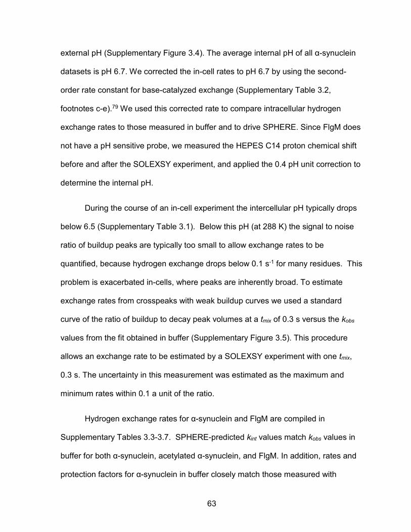
63

external pH (Supplementary Figure 3.4). The average internal pH of all α-synuclein

datasets is pH 6.7. We corrected the in-cell rates to pH 6.7 by using the second-

order rate constant for base-catalyzed exchange (Supplementary Table 3.2,

footnotes c-e).79 We used this corrected rate to compare intracellular hydrogen

exchange rates to those measured in buffer and to drive SPHERE. Since FlgM does

not have a pH sensitive probe, we measured the HEPES C14 proton chemical shift

before and after the SOLEXSY experiment, and applied the 0.4 pH unit correction to

determine the internal pH.

During the course of an in-cell experiment the intercellular pH typically drops

below 6.5 (Supplementary Table 3.1). Below this pH (at 288 K) the signal to noise

ratio of buildup peaks are typically too small to allow exchange rates to be

quantified, because hydrogen exchange drops below 0.1 s-1 for many residues. This

problem is exacerbated in-cells, where peaks are inherently broad. To estimate

exchange rates from crosspeaks with weak buildup curves we used a standard

curve of the ratio of buildup to decay peak volumes at a tmix of 0.3 s versus the kobs

values from the fit obtained in buffer (Supplementary Figure 3.5). This procedure

allows an exchange rate to be estimated by a SOLEXSY experiment with one tmix,

0.3 s. The uncertainty in this measurement was estimated as the maximum and

minimum rates within 0.1 a unit of the ratio.

Hydrogen exchange rates for α-synuclein and FlgM are compiled in

Supplementary Tables 3.3-3.7. SPHERE-predicted kint values match kobs values in

buffer for both α-synuclein, acetylated α-synuclein, and FlgM. In addition, rates and

protection factors for α-synuclein in buffer closely match those measured with

64

CLEANEX (Supplementary Table 3.3).112 The differences likely reflect differences in

buffer composition and extrapolation to pH 6.7.

In buffer, 26 α-synuclein residues give quantifiable exchange rates and seven

more rates can be estimated (Figure 3.1A, 3.2A, Supplementary Table 3.3). The

residues are distributed throughout the primary structure. Their protection factors are

all similar and less than two. The same is observed for α-synuclein in buffer

supplemented with 150 mM NaCl (Supplementary Table 3.3). Protection factors this

small indicate a lack of structure.102

In cells, nine α-synuclein residues give quantifiable rates, eight more rates

can be estimated, and an additional six qualitatively show exchange (Figures 3.1B,

3.2A, Supplementary Tables 3.2, 3.3). Rates in cells and in buffer are in reasonable

agreement with the values predicted by SPHERE. No protection factor is greater

than three (Figure 3.2B). There is no significant difference between the protection

factors, both measured and estimated, in cells and in buffer (two-tailed t-test with

unequal variance125, ρ > 0.07). The same is observed for acetylated α-synuclein.

There is no significant difference between protection factors in cells and buffer

(Supplementary Figure 3.6, Supplementary Tables 3.4, 3.5, two-tailed t-test with

unequal variance, ρ > 0.5). These observations indicate that α-synuclein, with or

without acetylation, remains disordered in the crowded bacterial cytoplasm.

65

Figure 3.1. 15NH/D-SOLEXSY spectra of α-synuclein in A) buffer and B) E. coli. Each panel is an overlay of the 0 ms (black) and 300 ms (red) mixing times. The contour levels in panels A and B are the same.

The activation energy

of amide proton exchange

was also measured

(Supplementary Table 3.8).

The means and their

standard deviations are 15 ±

3 kcal/mol in buffer and 17 ± 1 kcal/mol in cells. The activation energy used in

SPHERE is 17 kcal/mol.83,86 These observations lend further support our to

conclusion that α-synuclein has the properties of a disordered peptide in the E. coli

cytoplasm.

Turning to FlgM, 24 residues give quantifiable exchange rates in buffer

(Figure 3.3A, 3.4A, Supplementary Table 3.7). Significantly larger protection factors

(ρ < 0.002, two-tailed t-test with unequal variance) are observed for the 13 C-

terminal residues compared to the 11 N-terminal residues (means and their standard

deviations of 1.6 ± 0.3 and 0.5 ± 0.1, respectively). This observation suggests the

existence of some structure in the C-terminal region, consistent with chemical shift

data showing that the C-terminus forms transient α-helices in buffer.118,119 However,

66

Figure 3.2. α-Synuclein exhibits similar backbone amide hydrogen exchange rates in cells and in buffer (pH 6.7, 288 K). A) Rates from prediction (red),83,84,86 and from SOLEXSY data (blue, buffer; green, cells). Uncertainties in buffer are the standard deviation of 20 Monte Carlo noise simulations.99 Uncertainties for the in-cell data are the standard deviation of the mean from three or more trials (For T81 ad G93, the uncertainties are the range of two experiments.). Asymmetric error bars are shown for rates derived from the data in Supplementary Figure 3.5, as described in the text. In-cell rates without error bars are for residues that that exchange too slowly for reliable fits, or have overlapped decay peaks, and were assigned a rate of ≥ 0.2 s-1, the lower limit of SOLXESY. B) Protection factors (kint, predicted/kobs, buffer and kint,

predicted/kobs, cells). Uncertainties are from propagation of the uncertainties shown in panel A unless the rate was derived from Supplementary Figure 3.5. For those residues, the uncertainty reflects a range, as described in the text. The arrows denote residues for which only a maximum value can be assigned.

the protection factors from the C-terminal region were all <5, indicating an absence

of persistent structure.102 In summary, the agreement between the chemical shift

data and the hydrogen exchange data show that protection factors are a sensitive

measure of sparsely populated secondary structure.

67

Figure 3.3. 15NH/D-SOLEXSY spectra of FlgM in A) buffer and B) E. coli. Each panel is an overlay of the 0 ms (black) and 300 ms (red) mixing times. The contour levels in panels A and B are the same.

In cells, seven FlgM

residues give quantifiable

rates and four more

qualitatively show exchange

(Figure 3.3B, 3.4A,

Supplementary Tables 3.6,

3.7). The rates in cells are similar to those in buffer. For the N-terminus seven

residues can be quantified in cells and 11 in buffer. Protection factors for these

residues (Figure 3.4B) are the same in cells as they are in buffer (two-tailed t-test

with unequal variance, ρ > 0.1).

Discussion

Unfortunately, we cannot directly compare cell and buffer data from the C-

terminus of FlgM because C-terminal crosspeaks disappear in cells.106 However, the

smaller exchange rates in buffer and the absence of crosspeaks are both consistent

with the existence of a nascent C-terminal structure. Likewise, for both acetylated

and non-acetylated α-synuclein, crosspeaks from the first 12 residues and residues

37-41 show peak broadening inside cells (Supplementary Figure 3.7). This

broadening is likely due to conformational exchange involving a helical form that is

68

Figure 3.4. FlgM exhibits similar backbone amide hydrogen exchange rates in cells and in buffer (pH 6.7, 298 K). See the caption to Figure 3.1 for further information.

populated in buffer to ~17% for acetylated α-synuclein and slightly less for the non-

acetylated form.126,127 This conformational exchange is likely slowed in cells causing

broadening. A similar observation has been made for a folding intermediate of the

FF domain in cell lysates.40

Our data for α-synuclein and the N-terminal region of FlgM indicate that

disorder can persist in E. coli irrespective of the existence of hard-core repulsions,

i.e. macromolecular crowding.74,128 We have shown that measured exchange rates

in E. coli agree with both those obtained in buffer and those calculated based on

exchange rates of small, unstructured peptides. Data for the C-terminal region of

FlgM in buffer show that even small protection factors can be useful indicators of

sparsely populated structured states in disordered proteins. This work also has

69

implications for determining the stability of globular proteins in living cells.

Specifically, the data indicate that predicted rates from model peptides can be

applied to hydrogen exchange studies of globular proteins inside E. coli.61 Most

importantly, we have shown that protein disorder can persist under physiological

conditions and that the crowded cellular interior need not affect the structure of

disordered proteins.

Methods

Protein expression for in-cell NMR

Plasmids harboring the gene encoding FlgM (PMC64, ampicillin resistance)

or α-synuclein (pT7-7, ampicillin resistance) were transformed into Agilent BL21 DE3

Gold cells by heat-shock. For acetylated α-synuclein, plasmids harboring pNatB

(chloramphenicol resistance) and α-synuclein were co-transformed into Agilent BL21

DE3 Gold cells by electroporation. A single colony was used to inoculate a 5 mL

culture of Luria-Bertani media supplemented with 100 μg/mL ampicillin (FlgM or α-

synuclein) or 100 μg/mL ampicillin and 25 μg/mL chloramphenicol (pNatB/α-

synuclein). The culture was grown 37 °C. After 8 h, 50 μL of the saturated culture

was used to inoculate 50 mL of supplemented M9 media as described next.

For uniform labeling, M9 media (50 mM Na2HPO4, 20 mM KH2PO4, 9 mM

NaCl) was supplemented with 2 mg/mL 13C-glucose, 1 mg/mL 15NH4Cl, 100 μM

CaCl2, 2 mM MgSO4, 10 μg/mL thiamine and 10 μg/mL biotin, and 150 μg/mL

ampicillin (100 μg/mL ampicillin and 25 μg/mL chloramphenicol for pNatB/α-

synuclein). For glycine or threonine “unlabeling,” the media described above was

70

also supplemented with 1 mg/mL natural abundance glycine or 1.5 mg/mL natural

abundance threonine.129,130

For selective lysine/threonine enrichment, natural abundance glucose and

NH4Cl were used in the M9 media, which was also supplemented with 0.1 mg/mL

uniformly enriched 13C/15N threonine, 0.2 mg/mL uniformly 13C/15N enriched lysine

and 0.2 mg/mL natural abundance glycine were added.131,132

The 50 mL cultures were shaken (New Brunswick Scientific Innova I26, 225

rpm) at 37 °C overnight. The culture was diluted to 100 mL with supplemented M9

media and shaken until the optical density at 600 nm was at least 0.8. Isopropyl β-D-

1-thiogalactopyranoside (1 mM) was used to induce expression. After 4 h cells were

pelleted at 1000g and washed 3 times with 30 mL NMR buffer (100 mM HEPES, 35

mM bis-tris propane,133 50 μg/mL chloramphenicol, 100 μg/mL ampicillin, 50% D2O).

For pNatB/α-synuclein the buffer contained half the amount of chloramphenicol and

15 μg/mL rifampin. Chloramphenicol or rifampin is required to halt protein

expression prior to NMR. (Rifampin is required because the pNatB plasmid harbors

a gene for chloramphenicol resistance.) Cell pellets were resuspended in 100-200

μL of NMR buffer and loaded into a standard 5 mm NMR tube. Typical cell slurries

were 70% wet cells by volume.

Protein purification

Cell pellets were frozen after in-cell NMR experiments. For α-synuclein (with

or without acetylation) cells were lysed by boiling. Cell debris was removed by

centrifugation at 16000g. Using a GE AKTA FPLC, anion exchange (GE Q column,

71

50 mM Tris-HCl wash buffer, 50 mM Tris-HCl/1 M NaCl elute buffer, pH 7.5, 10-90%

gradient) and subsequent size exclusion chromatography (GE Superdex 75 column

eluted with non-supplemented M9, 0.5 ml/min flow rate) were used. SDS-PAGE was

used to assess purity. Purified protein was dialyzed against 17 MΩ cm-1 H2O for 4 h

at room temperature or overnight at 5 °C. After dialysis, the sample was flash frozen

in a dry-ice/ethanol bath and lyophilized.

FlgM was purified in a similar fashion except the cells were sonicated (Fisher

Scientific Sonic Dismembrator Model 500, 15% amplitude, 20 s, 67% duty cycle).

FlgM does not bind to anion exchange media.

LC-ESI-MS

Purified samples of α-synuclein were resuspended in 17 MΩ cm-1 H2O and

subjected to LC-ESI-MS using a Restek Viva C4 column (linear gradient from 0.1%

aqueous formic acid, 5% acetonitrile to 0.1% aqueous formic acid, 95% acetonitrile

over 15 m, followed by 5 m in the 95% eluant) coupled to an Agilent 6520 Accurate-

Mass Q-TOF running in positive ion mode. Deconvoluted masses of 15240 Da and

15280 Da were found for 13C/15N α-synuclein and 13C/15N acetylated α-synuclein,

respectively. This mass difference corresponds to the addition of an acetyl group

(~40 Da). No unmodified α-synuclein was observed when the protein was co-

expressed with pNatB, indicating 100% acetylation, consistent with previous work.134

pH determination

Purified α-synuclein (0.5 mM) was suspended in 50 mM citrate, 50 mM bis-tris

propane, 50 mM HEPES, 50 mM borate, 5% D2O, containing 0.1% DSS at various

72

pH values (adjusted by addition NaOH or HCl). Data were acquired at 288 K (pH:

3.0, 4.2, 5.3, 5.7, 6.0, 6.4, 6.6, 6.8, 7.0, 7.5, 7.8, 8.9) and 298 K (pH: 5.3, 6.1, 6.6,

7.0, 7.4, 7.9, 8.9) on either a 600 or 700 MHz Bruker Avance III HD spectrometer

equipped with a Bruker TCI cryoprobe. 13C-HSQC spectra were acquired using

sweep widths of 12 ppm in the 1H dimension and 200 ppm in the 13C dimension.

Four transients were collected using 512 complex points in t2 and 64 complex

increments in t1. Spectra were referenced to DSS at 0 ppm. Data were processed

with Topspin 3.2. The 1H chemical shifts of H50 13Cε1-1H and 13Cδ2-1H of α-synuclein

and HEPES were followed as a function of pH. The data were fit to a modified

Henderson-Hasselbach equation, � = ���� − ���������� ! "#$%&'(%)*, where δlow is the low pH

chemical-shift plateau and δhigh is the high plateau, n is the number of protons, and

pKa is the negative logarithm of the dissociation constant.135-137 Our pKa values (6.7

for H50 and 7.5 for HEPES) are similar to literature values (6.8 and 7.6,

respectively).123,124

Using a glass electrode (AgCl reference), buffers containing 5% and 50%

D2O and α-synuclein (0.5 mM) were adjusted to a pH reading of 6.9. The solutions

gave nearly identical proton chemical shifts for ε1 (7.984 ppm and 7.983 ppm) and

δ2 (7.074 ppm and 7.073 ppm), for 5 and 50% D2O. Thus, the H50 13Cε1 and 13Cδ1

protons are insensitive to the H/D isotope effect and 0.2 pH units were added to the

value obtained from the standard curve in solutions containing a 1:1 H2O:D2O

mixture to account for the H/D isotope effect on the electrode for a 50% D2O

solution.138,139 The C14 protons of HEPES, however, exhibit an isotope effect. In 5%

D2O the proton chemical shift is 3.117 ppm while in 50% D2O the chemical shift is

73

3.134 ppm. For this reason, a correction of -0.017 ppm was applied to values

obtained in 50% D2O to account for the deviation from the conditions used to acquire

the standard curve, then the 0.2 pH unit correction was added to the value obtained

from the standard curve.

NMR

In-cell samples were prepared as described above. For the buffer

experiments purified 13C-, 15N-enriched protein (final protein concentration of ~500

μM as judged by a Lowry assay using bovine serum albumin as the standard) was

added to NMR buffer (pH 6.7, minus antibiotics). One buffer experiment with α-

synuclein used NMR buffer plus 150 mM NaCl, to ensure minimal salt dependence

of exchange. In-cell data were acquired at 288 K (α-synuclein, acetylated α-

synuclein), and 298 K (FlgM, α-synuclein) with a 700 MHz Bruker Avance III HD

spectrometer running Topspin Version 3.2 and equipped with a Bruker TCI

cryoprobe. Buffer data were acquired at 288 K (α-synuclein, acetylated α-synuclein),

293 K (α-synuclein) and 298 K (FlgM, α-synuclein). An interleaved, modified52

SOLEXSY99 (Appendix 1) experiment with mixing times (tmix) of 0, 70, 140, 210, 300,

500, and 800 ms was used to measure hydrogen exchange rates. One in-cell

exchange experiment with α-synuclein used tmix of 0, 70, 150, 300, 700 ms in an

attempt to shorten the acquisition time and minimize pH changes. Sweep widths

were 7000 Hz and 2500 Hz in the 1H and 15N dimensions, respectively. 512 complex

points were collected in t2 with 128 TPPI points in t1 at each tmix. In buffer, 32

transients were acquired per increment. Forty transients were acquired for the in-cell

NMR experiments. Data acquisition required ~16 h per sample.

74

15N-1H and 13C-1H HSQC spectra were acquired before and after the

SOLEXSY experiment to assess sample integrity and pH. Four or eight transients

were collected using 512 complex points in t2 with 64 complex points in t1 for each

experiment. The sweep widths were 8500 Hz in 1H and either 2500 Hz or 34500 Hz

in the 15N or 13C dimension, respectively. For the in-cell samples, the cell slurry was

removed after the experiment and gently pelleted. The supernatant was removed,

diluted two- to three-fold, and placed in the spectrometer. A 15N-1H HSQC was

acquired to assess protein leakage.24 No leakage was observed (~μM detection

limit).

To ensure the pH associated with an in-cell SOLEXSY experiment was the

average of the values obtained from the bracketed 13C-1H HSQC spectra, an

experiment using α-synuclein was performed where 13C-1H HSQC spectra were

acquired as a function of time. These HSQC spectra bracketed a short SOLEXSY

(only tmix 0.3 s) experiment and an 15N-1H TROSY-HSQC experiment. This regimen

not only allowed us to determine that the pH drop was linear but also allowed

collection of single-plane SOLEXSY experiments where the pH drop was only

averaged over ~2.5 h instead of the ~16 h required for a complete SOLEXSY

experiment. This protocol allowed us to assess hydrogen exchange at discreet pH

values, instead of exchange averaged over a ~0.5 pH unit range.

Data processing

Data were processed with NMRPipe.104 t2 data were subjected to a cosine

squared bell function (512 complex points for buffer solutions and 256 complex

75

points for in-cell experiments) before zero-filling to 2048 points and Fourier

transformation. t1 data were linear predicted to 256 points before application of a

cosine squared bell function. Subsequent zero-filling to 1024 points and Fourier

transform yielded the final spectra. Spectra were peak picked and integrated using

the built-in nlinLS routine. Peak volumes were fitted as described.99 Published

assignments were used.118,119,140,141

76

Supplementary Information for Chapter 3

Supplementary Table 3.1. pH.

pH range Interior Exterior

Protein Enrichmenta Temperature (K) Time (h)b H50 ε1c H50 δ2c HEPESc α-synuclein 13C/15N 288 11 7.1 – 6.8 7.0 – 6.9 7.6 – 7.1

13C/15N 288 16 7.1 – 6.3 7.0 – 6.2 7.6 – 6.7

13C/15N 288 16 6.9 – 6.2 6.8 – 6.1 7.3 – 6.6 13C/15N 298 16 6.5 – 5.3 6.5 – ND 6.5 – 6.2 13C/15N, -G 288 16 ND 6.7 – 5.7 6.9 – 6.3 13C/15N, -T 288 16 6.8 – 6.1 6.7 – 5.9 6.9 – 6.4 +T/K 288 16 7.0 – 6.5 ND 7.6 – 6.9

Acetylated 13C/15N 288 16 6.8 – 6.3 6.7 – 6.1 7.2 – 6.6 α-synuclein 13C/15N 288 17 7.1 – 6.7 7.0 – 6.5 7.6 – 7.2

13C/15N 288 17 7.0 – 6.6 7.0 – 6.6 7.6 – 7.2 FlgM 13C/15N 298 16 NA NA 6.9 – 6.3

13C/15N 298 16 NA NA 6.9 – 6.3

13C/15N 298 16 NA NA 6.8 – 6.3

Footnotes

a Media 13C/15N: 13C-glucose and 15NH4Cl. 13C/15N, -G: 13C-glucose and 15NH4Cl plus natural abundance glycine. 13C/15N, -T: 13C-glucose and 15NH4Cl plus natural abundance threonine. +T/K: natural abundance glucose and NH4Cl plus 13C/15N enriched threonine and lysine.

b Duration of SOLEXSY experiment.

c pH before SOLEXSY experiment and pH after SOLEXSY experiment. pH values were obtained from 13C-1H HSQC spectra and the standard curves shown in Supplementary Figure 3.2. ND; not determined. NA; not applicable.

77

Supplementary Table 3.2. Triplicate α-synuclein in-cell data extrapolated to pH 6.7.

Residue kobs (s-1)a In-cell pHb logkobs pOH-c logkOH-

d kobs at pH 6.7 (s-1)e

G31 1.2 6.6 0.1 8.2 8.3 1.7 2.7 6.7 0.4 8.1 8.5 2.7

2.0 7.0 0.3 7.8 8.1 1.1 G67 1.5 6.6 0.2 8.2 8.4 2.1

2.8 6.7 0.4 8.1 8.5 2.8

2.2 7.0 0.3 7.8 8.2 1.2 G68 1.2 6.6 0.1 8.2 8.3 1.6

1.4 6.7 0.2 8.1 8.2 1.4 1.4 7.0 0.1 7.8 8.0 0.8

T81 1.5 6.8 0.2 8.0 8.2 1.3 0.3 6.2 -0.5 8.6 8.1 1.0

E83 0.3 6.6 -0.5 8.2 7.8 0.5 0.1 6.7 -0.9 8.1 7.2 0.1 0.7 7.0 -0.2 7.8 7.7 0.4

G86 1.7 6.6 0.2 8.2 8.5 2.4 3.0 6.7 0.5 8.1 8.6 3.0 3.6 7.0 0.6 7.8 8.4 2.0

T92 0.9 6.6 -0.04 8.2 8.2 1.3 1.6 6.7 0.2 8.1 8.3 1.6 3.3 7.0 0.5 7.8 8.4 1.9 0.7 6.2 -0.2 8.6 8.4 2.1

G93 1.6 6.6 0.2 8.2 8.4 2.2 3.0 7.0 0.5 7.8 8.3 1.7

N103 1.4 6.6 0.1 8.2 8.4 1.9 1.9 6.7 0.3 8.1 8.4 1.9 2.9 7.0 0.5 7.8 8.3 1.6 1.0 6.2 -0.02 8.6 8.6 3.0 0.9 6.6 -0.04 8.2 8.2 1.3

Footnotes

a From fitting SOLEXSY exchange curves. Cells were resuspended in 100 mM HEPES, 35 mM bis-tris propane, 50 μg/mL chloramphenicol, 100 μg/mL ampicillin, 288 K, 50% D2O.

b Average pH from the chemical shift of H50 ε1 or δ2 proton before and after the SOLEXSY experiment (Supplementary Figures 3.2 and 3.3).

c pOH- = pKW - pH; pKW = 14.79 (to account for 50% D2O, 288 K).

d Logarithm of the second-order rate constant for base-catalyzed exchange (kOH- = kobs/[OH-

]).

e kobs extrapolated to pH 6.7: 10(logkOH-pOH) = 10(logkOH-pKW+pH) = 10(logkOH-14.79+6.7) = 10(logkOH-8.09).

78

Supplementary Table 3.3. α-Synuclein exchange rates (s-1) and protection factors (PF).

Residue SPHEREa Bufferb Crokec Cellsd Buff PFe Cell PFe

G7 1.2 2.2 (1.4 - 3.8)f NR NDg 0.5 (0.3 - 0.9) ND L8 0.2 0.8 (0.1 - 1.6) 0.7 ± 0.1 ND 0.3 (0.1 - 2.0) ND S9 0.7 2.0 [2.2] ± 0.2 1.4 ± 0.4 ND 0.4 [0.3] ± 0.1 ND

T22 0.6 0.7 [1.1] ± 0.3 0.9 ± 0.1 1.6 (0.4 - 3.3)f 0.9 [0.5] ± 0.4 0.4 (0.2 - 1.5) K23 0.7 1.7 (0.4 - 2.8) NR 1.7 (0.4 - 3.3) 0.4 (0.3 - 1.8) 0.4 (0.2 - 1.8)

G31 0.9 1.2 [2.3] ± 0.2 NR 1.8 ± 0.4 0.8 [0.4] ± 0.1 0.5 ± 0.1 T33 0.6 1.6 (0.4 - 3.3) NR ≥ 0.2 0.4 (0.2 - 1.5) ≤ 3.0 K34 0.7 1.7 (0.4 - 3.3) NR 2.1 (1.4 - 4.0)h 0.4 (0.2 - 1.8) 0.3 (0.2 - 0.5) V40 0.1 0.4 [0.2] ± 0.2 0.3 ± 0.1 ND 0.3 [0.5] ± 0.2 ND G41 0.7 0.7 [0.6] ± 0.6 1.2 ± 0.2 ND 1.0 [1.2] ± 0.8 ND T44 0.6 0.5 [1.2] ± 0.1 1.1 ± 0.3 ≥ 0.2 1.1 [0.5] ± 0.2 ≤ 3.0 K45 0.7 1.2 ± 0.2i NR 2.1 (1.4 - 4.0) 0.6 ± 0.1 0.3 (0.2 - 0.5) V52 0.2 0.6 ± 0.2j NR ND 0.3 ± 0.1 ND A53 0.4 0.7 [0.7] ± 0.2 0.5 ± 0.1 ≥ 0.2 0.6 [0.6] ± 0.2 ≤ 1.8 T54 0.4 0.7 (0.1 - 1.0) 0.6 ± 0.1 ≥ 0.2 0.6 (0.4 - 4.0) ≤ 2.0 K60 0.7 1.4 (0.4 - 2.7) 0.7 ± 0.1 2.1 (1.4 - 4.0) 0.5 (0.3 - 1.8) 0.3 (0.2 - 0.5)

N65 2.4 1.6 [1.4] ± 0.1 NR ND 1.5 [1.7] ± 0.1 ND V66 0.2 0.9 ± 0.1 NR ≥ 0.2 0.2 ± 0.1 ≤ 1.0 G67 0.7 0.4 [1.8] ± 0.1 0.8 ± 0.2 2.0 ± 0.4 1.8 [0.4] ± 0.5 0.4 ± 0.1 G68 1.4 1.4 ± 0.2 0.8 ± 0.2 1.3 ± 0.3 1.0 ± 0.1 1.1 ± 0.2

V70 0.1 0.4 ± 0.2 NR ≥ 0.2 0.3 ± 0.2 ≤ 0.5 V74 0.2 0.6 ± 0.2 0.7 ± 0.1 ND 0.3 ± 0.1 ND A76 0.8 1.7 ± 0.6 0.9 ± 0.2 ND 0.5 ± 0.2 ND T81 0.6 1.0 [1.2] ± 0.3 1.1 ± 0.2 1.2 ± 0.3 0.6 [0.5] ± 0.2 0.5 ± 0.1 E83 0.1 0.5 [0.7] ± 0.1 NR 0.3 ± 0.1 0.2 [0.1] ± 0.1 0.3 ± 0.1 G84 0.7 1.4 ± 0.3 0.8 ± 0.2 ND 0.5 ± 0.1 ND G86 0.9 1.8 [2.1] ± 0.6 0.7 ± 0.2 2.5 ± 0.3 0.5 [0.4] ± 0.2 0.4 ± 0.1 T92 0.4 1.6 [1.1] ± 0.5 0.7 ± 0.2 1.7 ± 0.2 0.3 [0.4] ± 0.1 0.2 ± 0.1 G93 1.5 1.9 ± 0.1 1.2 ± 0.4 2.0 ± 0.5 0.8 ± 0.1 0.8 ± 0.1

K97 0.6 1.2 ± 0.2 NR 2.1 (1.4 - 4.0) 0.5 ± 0.1 0.3 (0.2 - 0.4) N103 2.0 1.1 [2.4] ± 0.1 0.8 ± 0.3 2.0 ± 0.3 1.8 [0.8] ± 0.2 1.0 ± 0.2 Q109 0.3 0.6 ± 0.2 0.5 ± 0.1 0.6 (0.1 - 1.0) 0.5 ± 0.2 0.5 (0.3 - 3.0) S129 0.7 0.6 ± 0.2 0.4 ± 0.1 1.4 (0.2 - 2.7) 1.2 ± 0.4 0.5 (0.3 - 3.5)

Footnotes

a Calculated with the online server SPHERE86 using the PDLA rate basis, pHmeter 6.3, 100% D2O and the amino acid sequence of α-synuclein.83,84,86 Rates from SPHERE match hand-calculated rates for 1:1 H2O:D2O buffer.52

79

b From fitting SOLEXSY exchange curves (pH 6.7, 100 mM HEPES, 35 mM bis-tris propane, 288 K, 50% D2O). Uncertainties are from Monte Carlo noise estimation. Values in brackets are from the same buffer plus 0.15 M NaCl (uncertainties ≤0.6 s-

1).

c CLEANEX data from Croke, et al. (pH 7.4, 20 mM phosphate, 288 K).112 Converted to base-catalyzed rates using pKW of 14.44 (pOH 7.04, to account for 10% D2O) followed by extrapolation to pH 6.7 using a pKW of 14.79 (pOH 8.09, to account for 50% D2O).101 Uncertainties <0.1 were set to 0.1. NR; not reported.

d From fitting SOLEXSY exchange curves and subsequent extrapolation to pH 6.7 using a pKW of 14.79 (pOH 8.09, to account for 50% D2O).101 Uncertainties are the standard deviations of the mean. Uncertainty for T81 and G93 are the range from two experiments. Cells were resuspended in 100 mM HEPES, 35 mM bis-tris propane, 50 μg/mL chloramphenicol, 100 μg/mL ampicillin, 50% D2O, 288 K. Rates of ≥0.2 s-1 were assumed for residues that exhibit a buildup peak at tmix 0.3 s whose decay peak overlapped another crosspeak.

e Calculated by dividing the rates from SPHERE by the rates in buffer or in cells. Uncertainties are from error propagation. Uncertainties <0.1 were set to 0.1. Protection factors in brackets are from the same buffer plus 0.15 M NaCl.

f Values estimated from the linear fit shown in Supplementary Figure 3.5 using the ratio of the volumes of buildup to decay peaks at a tmix of 0.3 s. Uncertainty (in parentheses) are the maximum and minimum rates within 0.1 units of this ratio as shown in the figure.

g ND: not determined due to crosspeak overlap or broadening.

h K34 overlaps with K45 and K97 in cells, yielding one exchange rate.

i In buffer K45 and K97 overlap, yielding one exchange rate.

j In buffer V52 and V74 overlap, yielding one exchange rate.

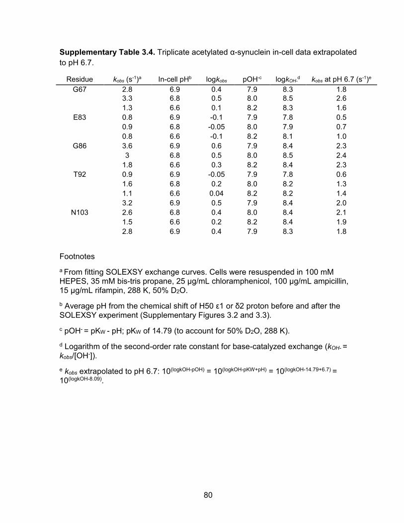
80

Supplementary Table 3.4. Triplicate acetylated α-synuclein in-cell data extrapolated to pH 6.7.

Residue kobs (s-1)a In-cell pHb logkobs pOH-c logkOH-

d kobs at pH 6.7 (s-1)e

G67 2.8 6.9 0.4 7.9 8.3 1.8 3.3 6.8 0.5 8.0 8.5 2.6

1.3 6.6 0.1 8.2 8.3 1.6 E83 0.8 6.9 -0.1 7.9 7.8 0.5

0.9 6.8 -0.05 8.0 7.9 0.7 0.8 6.6 -0.1 8.2 8.1 1.0

G86 3.6 6.9 0.6 7.9 8.4 2.3 3 6.8 0.5 8.0 8.5 2.4 1.8 6.6 0.3 8.2 8.4 2.3

T92 0.9 6.9 -0.05 7.9 7.8 0.6 1.6 6.8 0.2 8.0 8.2 1.3 1.1 6.6 0.04 8.2 8.2 1.4 3.2 6.9 0.5 7.9 8.4 2.0

N103 2.6 6.8 0.4 8.0 8.4 2.1 1.5 6.6 0.2 8.2 8.4 1.9 2.8 6.9 0.4 7.9 8.3 1.8

Footnotes

a From fitting SOLEXSY exchange curves. Cells were resuspended in 100 mM HEPES, 35 mM bis-tris propane, 25 μg/mL chloramphenicol, 100 μg/mL ampicillin, 15 μg/mL rifampin, 288 K, 50% D2O.

b Average pH from the chemical shift of H50 ε1 or δ2 proton before and after the SOLEXSY experiment (Supplementary Figures 3.2 and 3.3).

c pOH- = pKW - pH; pKW of 14.79 (to account for 50% D2O, 288 K).

d Logarithm of the second-order rate constant for base-catalyzed exchange (kOH- = kobs/[OH-]).

e kobs extrapolated to pH 6.7: 10(logkOH-pOH) = 10(logkOH-pKW+pH) = 10(logkOH-14.79+6.7) = 10(logkOH-8.09).

81

Supplementary Table 3.5. Acetylated α-synuclein exchange rates (s-1) and protection factors (PF).

Residue SPHEREa Bufferb Cellsc Buffer PFd Cell PFd

D2 0.3 0.8 ± 0.2 NDe 0.4 ± 0.1 ND G7 1.2 1.9 ± 0.4 ND 0.6 ± 0.1 ND

S9 0.7 2.4 ± 0.1 ND 0.3 ± 0.1 ND T22 0.6 1.5 ± 0.3 ND 0.4 ± 0.1 ND G31 0.9 1.1 ± 0.1 1.1 (0.3 - 2.7)f 0.8 ± 0.1 0.8 (0.3 - 3.0)

T33 0.6 2.4 (0.5 - 5.0) ND 0.3 (0.1 - 1.2) ND K34g 0.7 1.2 ± 0.3 ≥ 0.2 0.6 ± 0.2 ≤ 3.5 V40 0.1 0.6 ± 0.3 ND 0.2 ± 0.1 ND G41 0.7 0.9 ± 0.1 ND 0.8 ± 0.1 ND T44 0.6 1.1 ± 0.3 ND 0.5 ± 0.1 ND K45 0.7 1.2 ± 0.3 ≥ 0.2 0.6 ± 0.2 ≤ 3.5 A53 0.4 0.9 ± 0.2 ND 0.4 ± 0.1 ND T54 0.4 0.9 (0.1 - 1.8) ND 0.4 (0.2 - 4.0) ND V66 0.2 0.8 ± 0.1 ND 0.3 ± 0.1 ND G67 0.7 0.3 ± 0.1 2.0 ± 0.3 0.4 ± 0.1 0.4 ± 0.1 T81 0.6 1.2 (0.3 - 2.7) 0.7 (0.1 - 1.6) 0.5 (0.2 - 2.0) 0.9 (0.4 - 6.0) E83 0.1 0.1 ± 0.1 0.7 ± 0.2 1.0 ± 1.0 0.1 ± 0.1 G84 0.7 1.3 ± 0.3 ND 0.5 ± 0.1 ND G86 0.9 1.7 ± 0.1 2.3 ± 0.1 0.5 ± 0.1 0.4 ± 0.1 T92 0.4 0.3 ± 0.1 1.1 ± 0.3 1.3 ± 0.4 0.4 ± 0.1 G93 1.5 2.7 ± 0.3 3.2 (3.0 - 4.0)h 0.6 ± 0.1 0.5 (0.4 - 0.5)

K97 0.6 1.2 ± 0.3 ≥ 0.2 0.5 ± 0.1 ≤ 3.0 N103 2.0 0.7 ± 0.1 2.0 ± 0.1 2.9 ± 0.4 1.0 ± 0.1 Q109 0.3 0.6 ± 0.3 0.7 (0.1 - 1.0) 0.5 ± 0.3 0.4 (0.3 - 3.0) S129 0.7 0.2 ± 0.2 0.5 (0.1 - 1.0) 3.5 ± 3.5 1.4 (0.7 - 7.0)

Footnotes

a Calculated with the online server SPHERE86 using the PDLA rate basis, pHmeter 6.3, 100% D2O, a blocked N-terminus and the amino acid sequence of α-synuclein.83,84,86

b From fitting SOLEXSY exchange curves (pH 6.7, 100 mM HEPES, 35 mM bis-tris propane, 288 K, 50% D2O). Uncertainties are from Monte Carlo noise estimation.

c From fitting SOLEXSY exchange curves and subsequent extrapolation to pH 6.7 using a pKW of 14.79 (pOH 8.09, to account for 50% D2O).101 Uncertainties are the standard deviations of the mean. Cells were resuspended in 100 mM HEPES, 35 mM bis-tris propane, 25 μg/mL chloramphenicol, 100 μg/mL ampicillin, 15 μg/mL rifampin, 50% D2O, 288 K. A rate of ≥0.2 s-1 were assumed for residues that exhibit a buildup peak at tmix 0.3 s whose decay peak overlapped another crosspeak.

82

d Calculated by dividing the rates from SPHERE by the rates in buffer or in cells. Uncertainties are from error propagation. Uncertainties <0.1 were set to 0.1.

e ND: not determined due to crosspeak overlap or broadening.

f Values estimated from the linear fit shown in Supplementary Figure 3.5 using the ratio of the volumes of buildup to decay peaks at a tmix of 0.3 s. Uncertainty (in parentheses) is the maximum and minimum rates within 0.1 units of this ratio as shown in the figure.

g K34 overlaps with K45 and K97 in cells and buffer, yielding one exchange rate.

h Values estimated from the linear fit shown in Supplementary Figure 3.5 using the ratio of the volumes of buildup to decay peaks at a tmix of 0.3 s. Uncertainty (in parentheses) is the closest rates to ratio.

83

Supplementary Table 3.6. Triplicate FlgM in-cell data extrapolated to pH 6.7.

Residue kobs (s-1)a In-cell pHb logkobs pOH-c logkOH-

d kobs at pH 6.7 (s-1)e

E19 0.2 6.2 -0.7 8.2 7.5 0.7 0.9 6.2 -0.1

8.2 8.2 2.8

0.9 6.2 -0.1 8.2 8.2 2.7 S21 1.6 6.2 0.2 8.2 8.4 5.1

0.6 6.2 -0.2 8.2 8.0 1.9 0.5 6.2 -0.3 8.2 7.9 1.5

T23 0.4 6.2 -0.4 8.2 7.8 1.3 1.0 6.2 0.0 8.2 8.2 3.1 0.8 6.2 -0.1 8.2 8.1 2.5

A36 1.1 6.2 0.03 8.2 8.3 3.4 1.1 6.2 0.04 8.2 8.3 3.4 0.9 6.2 -0.05 8.2 8.2 2.8

T37 1.6 6.2 0.2 8.2 8.4 5.1 1.1 6.2 0.05 8.2 8.3 3.5 0.9 6.2 -0.1 8.2 8.2 2.8

T6/T20/S40f 0.5 6.2 -0.3 8.2 8.0 1.7 0.6 6.2 -0.2 8.2 8.0 1.8 0.5 6.2 -0.3 8.2 7.9 1.6

Footnotes

a From fitting SOLEXSY exchange curves. Cells were resuspended in 100 mM HEPES, 35 mM bis-tris propane, 50 μg/mL chloramphenicol, 100 μg/mL ampicillin, 298 K, 50% D2O.

b Average pH from chemical shift of HEPES C14 protons (minus 0.4 pH units, see Supplementary figures 3.2 and 3.4) from 13C-1H HSQCs before and after the SOLEXSY experiment.

c pOH- = pKW - pH; pKW of 14.43 (to account for 50% D2O, 298 K).

d Logarithm of the second-order rate constant for base-catalyzed exchange (kOH- = kobs/[OH-]).

e kobs extrapolated to pH 6.7: 10(logkOH-pOH-) = 10(logkOH-pKW+pH) = 10(logkOH-14.43+6.7) = 10(logkOH-7.73).

f T6, T20 and S40 crosspeaks are overlapped.

84

Supplementary Table 3.7. FlgM exchange rates (s-1) and protection factors (PF).

Residue SPHEREa Bufferb Cellsc Buffer PFd Cell PFd

T6 1.9 3.9 ± 0.1 1.7 ± 0.1e 0.5 ± 0.1 1.1 ± 0.1 V12 0.2 0.6 ± 0.2 NDf 0.3 ± 0.1 ND

V15 0.4 1.2 ± 0.4 ≥ 0.2 0.3 ± 0.1 ≤ 2.0 Q16 1.1 2.1 ± 0.1 ≥ 0.2 0.5 ± 0.1 ≤ 5.5 E19 0.7 1.7 ± 0.1 2.0 ± 0.7 0.4 ± 0.1 0.4 ± 0.1 T20 0.8 3.0 ± 0.1g 1.7 ± 0.1 0.3 ± 0.1 0.5 ± 0.1 S21 5.1 ND 2.8 ± 1.2 ND 1.8 ± 0.8 T23 0.8 1.0 ± 0.1 ≥ 0.2 0.8 ± 0.1 ≤ 4.0

E31 0.7 2.9 ± 0.1 ≥ 0.2 0.2 ± 0.1 ≤ 3.5 A36 1.4 1.5 ± 0.1 3.2 ± 0.2 0.9 ± 0.1 0.4 ± 0.1 T37 1.2 3.0 ± 0.1 3.8 ± 0.7 0.4 ± 0.1 0.3 ± 0.1 S40 3.2 3.0 ± 0.1 1.7 ± 0.1 1.1 ± 0.1 1.9 ± 0.1

S44 2.0 0.6 ± 0.4 ND 3.3 ± 2.2 ND Q47 1.6 1.0 ± 0.2 ND 1.6 ± 0.3 ND A48 2.2 1.1 ± 0.1 ND 2.0 ± 0.2 ND K49 1.3 0.4 ± 0.1 ND 3.3 ± 0.8 ND G54 1.5 1.3 ± 0.1 ND 1.2 ± 0.1 ND A65 1.0 1.6 ± 0.1 ND 0.6 ± 0.1 ND T68 1.5 1.7 ± 0.2 ND 0.9 ± 0.1 ND G73 5.3 3.0 ± 0.4 ND 1.8 ± 0.2 ND G80 4.0 2.4 ± 0.2 ND 1.7 ± 0.1 ND A83 0.8 1.4 ± 0.4 ND 0.6 ± 0.2 ND S92 5.1 3.5 ± 0.5 ND 1.5 ± 0.2 ND L94 0.4 0.8 ± 0.2 ND 0.5 ± 0.1 ND S96 5.1 4.1 ± 0.2 ND 1.2 ± 0.1 ND

Footnotes

a Calculated with the online server SPHERE86 using the poly-DL-alanine rate basis (PDLA) at pHmeter 6.3 in 100% D2O and the amino acid sequence of FlgM.83,84,86

b From fitting SOLEXSY exchange curves (pH 6.7, 100 mM HEPES, 35 mM bis-tris propane, 298 K, 50% D2O). Uncertainties are from Monte Carlo noise estimation. The exchange rate for S21 cannot be measured in buffer because its buildup crosspeak overlaps the decay crosspeak of S44.

c From fitting SOLEXSY exchange curves and subsequent extrapolation to pH 6.7 using a pKW of 14.43 (pOH 7.73, to account for 50% D2O).101. Uncertainties are the standard deviations of the mean from three trials. Cells were resuspended in 100 mM HEPES, 35 mM bis-tris propane, 50 μg/mL chloramphenicol, 100 μg/mL ampicillin, 50% D2O, 298 K. Rates of ≥0.2 s-1 were assumed for residues that exhibit a buildup peak whose decay peak overlapped another crosspeak.

85

d Calculated by dividing the rates from SPHERE by the rates in buffer or in cells. Uncertainties are from error propagation. Uncertainties <0.1 were set to 0.1.

e T6, T20 and S40 overlap in cells and yield one exchange rate.

f ND: not determined due to crosspeak overlap or broadening.

g T20 and S40 overlap in buffer and yield one exchange rate.

86

Supplementary Table 3.8. Activation energy of amide proton exchange from α-synuclein data.

In buffer In cells

Residue

kobs (s-1) 288 Ka

kobs (s-1) 293 Kb

kobs (s-1) 298 Kc

Ea (kcal/mol)

kobs (s-1) 288 Ka

kobs (s-1) 298 Kd

Ea (kcal/mol)

G31 1.2 ± 0.2 1.8 ± 0.4 2.1 ± 0.1 10 1.8 ± 0.4 5.7 ± 0.6 20 G67 0.4 ± 0.1 0.5 ± 0.2 1.9 ± 0.1 26 2.0 ± 0.4 5.0 ± 0.6 16 G68 1.4 ± 0.2 1.4 ± 0.3 2.6 ± 0.2 11 1.3 ± 0.3 4.4 ± 1.9 21 G86 1.8 ± 0.6 2.6 ± 0.1 3.4 ± 0.1 11 2.5 ± 0.3 5.0 ± 0.6 12 N103 1.1 ± 0.1 1.3 ± 0.1 2.6 ± 0.1 15 2.0 ± 0.5 5.0 ± 1.3 16

Average 15 ± 3e 17 ± 1e

Footnotes

a From Supplementary Table 3.3.

b From fitting SOLEXSY exchange curves (pH 6.7, 100 mM HEPES, 35 mM bis-tris propane, 293 K, 50% D2O). Uncertainties are from Monte Carlo noise estimation.

c From fitting SOLEXSY exchange curves (pH 6.7, 100 mM HEPES, 35 mM bis-tris propane, 293 K, 50% D2O). Uncertainties are from Monte Carlo noise estimation.

d From fitting SOLEXSY exchange curves and subsequent extrapolation to pH 6.7 using a pKW of 14.43 (pOH 7.73, to account for 50% D2O).101 Uncertainties are from Monte Carlo noise estimation. Cells were resuspended in 100 mM HEPES, 35 mM bis-tris propane, 50 μg/mL chloramphenicol, 100 μg/mL ampicillin, 50% D2O, 298 K.

e Uncertainty is the standard deviation of the mean.

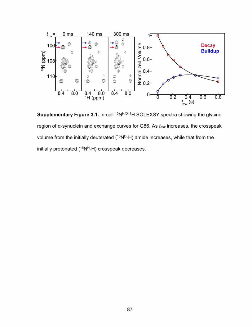
87

Supplementary Figure 3.1. In-cell 15NH/D-1H SOLEXSY spectra showing the glycine

region of α-synuclein and exchange curves for G86. As tmix increases, the crosspeak

volume from the initially deuterated (15ND-H) amide increases, while that from the

initially protonated (15NH-H) crosspeak decreases.

88

Supplementary Figure 3.2. Titration curves in buffer. The chemical shift of the 13Cε1

(○) and 13Cδ2 (○) protons from H50 of α-synuclein and the C14 protons of HEPES80

(○) are plotted versus pH. The fitted pKa values are shown next to the curves.

89

Supplementary Figure 3.3. Acidification of the cytoplasm over the ~16 h time

course of the SOLEXSY experiment. Titration curve is based on the proton

chemical shift from α-synuclein H50 13Cε1 (○) at 288 K (Supplementary Figure 3.2).

The chemical shift in cells was measured before (□) and after (x) each in-cell

experiment. The inset shows the 13Cε1 proton crosspeaks from 13C-1H HSQC spectra

before (black) and after (red) the SOLEXSY experiment.

90

Supplementary Figure 3.4. Acidification of the cytoplasm during the SOLEXSY

experiment (pHexternal - pHinternal = ~0.4 units). The chemical shifts from HEPES and

H50 of α-synuclein were measured as a function of time. The C14 protons of

HEPES (○) assess external pH,124 while the ε1 (○) and δ2 (○) protons of H50 assess

internal pH.

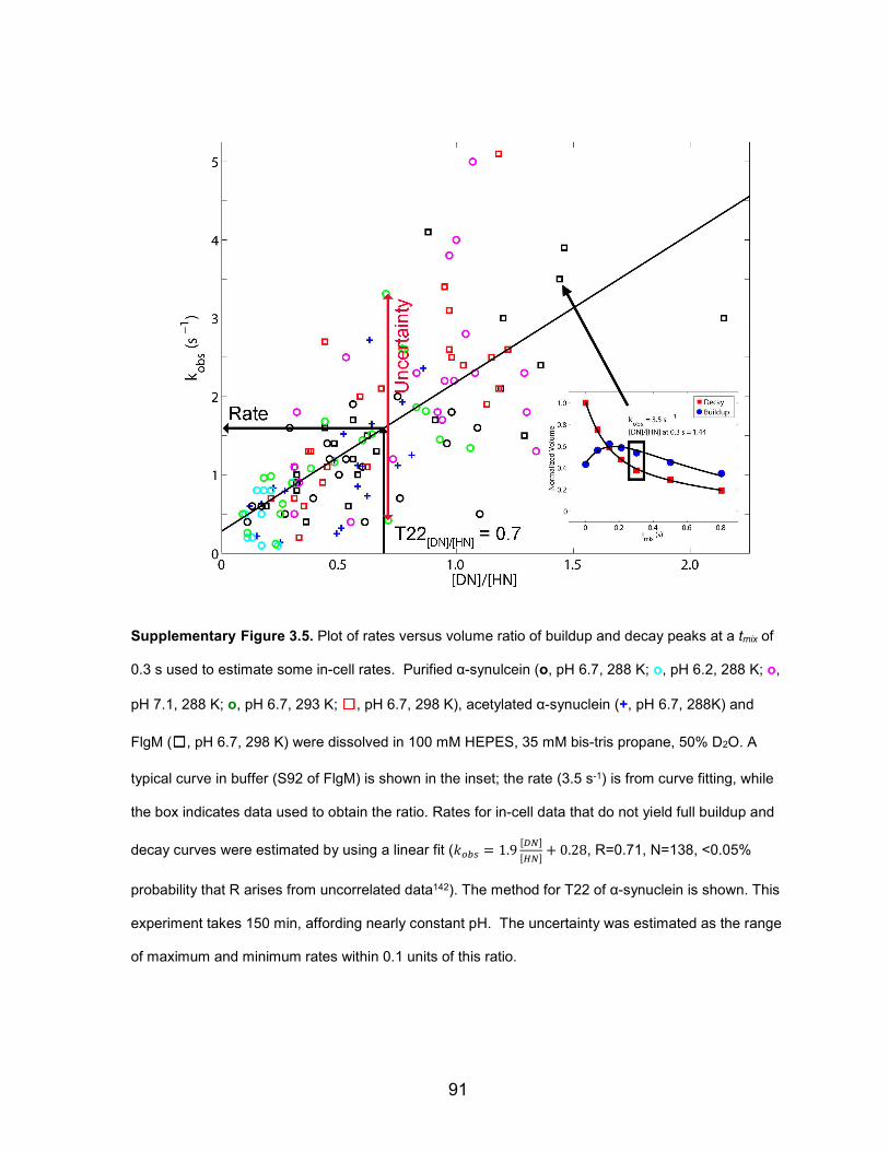
91

Supplementary Figure 3.5. Plot of rates versus volume ratio of buildup and decay peaks at a tmix of

0.3 s used to estimate some in-cell rates. Purified α-synulcein (o, pH 6.7, 288 K; o, pH 6.2, 288 K; o,

pH 7.1, 288 K; o, pH 6.7, 293 K; ☐☐☐☐, pH 6.7, 298 K), acetylated α-synuclein (+, pH 6.7, 288K) and

FlgM (☐☐☐☐, pH 6.7, 298 K) were dissolved in 100 mM HEPES, 35 mM bis-tris propane, 50% D2O. A

typical curve in buffer (S92 of FlgM) is shown in the inset; the rate (3.5 s-1) is from curve fitting, while

the box indicates data used to obtain the ratio. Rates for in-cell data that do not yield full buildup and

decay curves were estimated by using a linear fit (+�,- = 1.9 12341534 + 0.28, R=0.71, N=138, <0.05%

probability that R arises from uncorrelated data142). The method for T22 of α-synuclein is shown. This

experiment takes 150 min, affording nearly constant pH. The uncertainty was estimated as the range

of maximum and minimum rates within 0.1 units of this ratio.

92

N-terminus (pI 9.5) B -Ac 1MDVFMKGLSKAKEGVVAAAEKTKQGVAEAA30 C -Ac MDVFMKGLSKAKEGVVAAAEKTKQGVAEAA B +Ac MDVFMKGLSKAKEGVVAAAEKTKQGVAEAA C +Ac MDVFMKGLSKAKEGVVAAAEKTKQGVAEAA B -Ac 31GKTKEGVLYVGSKTKEGVVHGVATVAEKTK60 C -Ac GKTKEGVLYVGSKTKEGVVHGVATVAEKTK B +Ac GKTKEGVLYVGSKTKEGVVHGVATVAEKTK C +Ac GKTKEGVLYVGSKTKEGVVHGVATVAEKTK

NAC (pI 4.5) B -Ac 61EQVTNVGGAVVTGVTAVAQKTVEGAGSIAAATGFV95 C -Ac EQVTNVGGAVVTGVTAVAQKTVEGAGSIAAATGFV B +Ac EQVTNVGGAVVTGVTAVAQKTVEGAGSIAAATGFV C +Ac EQVTNVGGAVVTGVTAVAQKTVEGAGSIAAATGFV

C-terminus (pI 3.8) B -Ac 96KKDQLGKNEEGAPQEGILEDMPVDPDNEAYEMPSEEGYQDYEPEA140 C -Ac KKDQLGKNEEGAPQEGILEDMPVDPDNEAYEMPSEEGYQDYEPEA B +Ac KKDQLGKNEEGAPQEGILEDMPVDPDNEAYEMPSEEGYQDYEPEA C +Ac KKDQLGKNEEGAPQEGILEDMPVDPDNEAYEMPSEEGYQDYEPEA

Supplementary Figure 3.6. Hydrogen exchange in α-synuclein (pI 4.7) in cells (C)

and in buffer (B) with (+) and without (-) acetylation. Residues whose crosspeaks

show hydrogen exchange are in red. Underlined residues are quantifiable (i.e., give

complete SOLEXSY buildup and decay curves). Residues whose crosspeaks are

broadened (likely due to chemical exchange) are in blue. Residues that show

hydrogen exchange at high pH, and probable chemical exchange as the cellular pH

decreases are shown in green. Residues that are overlapped or broadened such

that exchange cannot be observed are in black.

93

CHAPTER 4: IN-CELL THERMODYNAMICS ESTABILISHES NEW ROLES FOR PROTEIN SURFACES

Original citation: Smith AE, Zhou LZ, Gorensek AH, Senske M, Pielak GJ. submitted

Abstract

There is abundant, physiologically-relevant knowledge about protein cores;

they are hydrophobic,143 exquisitely well packed,144 and nearly all hydrogen bonds

are satisfied.145 With rare exceptions,19,21,63 however, physiological understanding of

protein surfaces, which expose charged and polar groups to the environment,

remains elusive because proteins are almost exclusively studied in vitro in the

simple conditions of water and buffer. Here, we establish the essential physiological

roles played by protein surfaces by measuring the equilibrium thermodynamics and

kinetics of protein folding in the complex environment of living cells, where the

concentration of macromolecules exceeds 200 g/L.1 19F NMR data on the globular 7-

kDa N-terminal SH3 domain of Drosophila signal transduction protein drk (SH3)

acquired inside E. coli show that charge-charge interactions are fundamental to

protein stability and folding kinetics. Our results contradict predictions from accepted

theories of macromolecular crowding146,147 and show that cosolutes commonly used

94

to mimic the cellular interior do not yield physiologically relevant information. As

such, we provide the foundation for a complete picture of protein chemistry in cells.

95

Introduction

Classic theories about the effects of complex environments consider only

hard-core repulsions and so predict purely entropically-driven protein

stabilization.128,146 Here, we test this idea in living cells. SH3 exists in a dynamic

equilibrium between the folded state and the unfolded ensemble.148 This two-

state behavior is ideal for NMR-based studies of folding.18 5-Fluorotryptophan

labeled29 SH3 exhibits only two 19F resonances: one from the folded state, the

other from the unfolded ensemble (Figure 4.1a).149 The area under each

resonance is proportional to its population, pf and pu, respectively. These

populations are used to quantify protein stability via the modified standard state

free energy of unfolding, ∆��° = −:;<= �>�?, where R is the gas constant and T is

the absolute temperature. Furthermore, the width at half height of each

resonance is proportional to the transverse relaxation rate, which is an

approximate measure of intermolecular interactions.98,100,150 Thus, this simple

system yields both quantitative thermodynamic knowledge and information about

interactions involving surfaces of the folded state and the unfolded ensemble.

Results and Discussion

To assess the enthalpic (∆��∘) and entropic (∆��∘) components of stability

we measured the temperature dependence of ∆��°. The data were fitted to the

integrated Gibbs-Helmholtz equation,151 assuming a constant heat capacity of

unfolding, ∆��,�∘ :

96

∆��° = ∆��,@AB° − ;∆��,@AB° + ∆��,�° C; − ;@AB − ; ln ;;@ABF,

where, ;@AB, is the melting temperature, ;G (where pf = pu), or the temperature of

maximum stability, ;- (where ∆��∘ = 0).151 In buffer at pH 7.2 and 298 K, ∆��° is

0.52 ± 0.03 kcal/mol, ∆��∘ is 10 ± 1 kcal/mol and a ;∆��∘ is 10 ± 1 kcal/mol

(Figure 4.1c, Supplementary Tables 4.1 and 4.2).

Spectra were then acquired in E. coli (Figure 4.1b). Both ;G and ∆��°

decreased relative to buffer (Figure 4.1c, Supplementary Tables 4.1 and 4.2),

consistent with other studies,58,63,152,153 but inconsistent with theory.146,147

Furthermore, the stability decrease (0.50 ± 0.06 kcal/mol at 298 K) arises from a

2 ± 1 kcal/mol decrease to ∆��∘ (Supplementary Table 4.3), which is also

inconsistent with theory.

The source of the inconsistency can be seen from the width of the

resonances. The resonance from both the folded state and the unfolded

ensemble are broader in cells than in buffer (Figure 4.1a, b, Supplementary

Table 4.2), suggesting the presence of weak, attractive intermolecular

interactions of SH3 with other cytoplasmic components.150 This finding is

consistent with the existence of nonspecific, attractive surface interactions, which

are absent from simple theory.128 The key observation is that the resonance from

the unfolded ensemble is twelve-fold broader compared to buffer, while the

folded state resonance is broadened only four-fold. The unfolded ensemble is

more affected because it exposes more surface than the folded state,154

97

suggesting that the enthalpic destabilization arises from attractive interactions

between the unfolded ensemble and the cytoplasm.

Figure 4.1. The intracellular environment destabilizes SH3 relative to buffer. 19F spectra acquired at 298 K, in buffer (a) and in cells (b). The blue trace is from the post-experiment supernatant and shows that the red spectrum arises from protein inside cells. c) Stability curves in buffer (black), in cells (red) and in 100 g/L urea (magenta). Error bars in buffer are smaller than the labels and represent the standard deviation of three independent trials. Error bars for the in-cell data at 273 K, 298 K and 313 K represent the standard deviation of three independent trials. d-f) Stability in buffer (black) and solutions of 100 g/L BSA (blue) and

98

lysozyme (red). The curve for buffer from panel c is reproduced in d. The net charges on SH3, BSA and lysozyme (based on sequence) are shown. Error bars for the in vitro crowded 298 K data represent the standard deviation from three trials. Analysis of uncertainties are discussed in Methods. Appearance of new resonances in the pH 3 BSA sample prevented extraction of thermodynamic parameters.

To explore the enthalpic component, we performed in vitro experiments at

pH 7.2, 5.4 and 3.0 in 100 g/L solutions of protein cosolutes with different net

charges (Figure 4.1d-f). SH3 (pIcalc 5) and bovine serum albumin (BSA, 66 kDa,

pIcalc 6) change from polyanions to polycations over this pH range, but lysozyme

(14 kDa, pIcalc 9) remains a polycation.

At pH 7.2, lysozyme destabilized SH3 (ΔΔ��,HIJ K° = -0.92 ± 0.03; Figure

4.1d) and broadened its resonances (Figure 4.2a, Supplementary Table 4.2). We

attribute both effects primarily to attractive charge-charge interactions between

the protein surfaces. Consistent with this idea, adding 0.15 M NaCl to screen the

charge-charge interaction, diminished both the destabilization (ΔΔ��,HIJ K° = -0.70

± 0.03) and line width (Supplementary Table 4.2). BSA, which has the same net

charge as SH3 at this pH, was slightly stabilizing (ΔΔ��,HIJ K° = 0.09 ± 0.06) and

accompanied by weak broadening, as expected for proteins having the same net

charge.128 An explanation for the modest stabilization is that BSA exposes a

distribution of positive and negative charges, partially offsetting the net charge-

charge repulsion.

At pH 5.4 (Figure 4.1e), SH3 is a polyanion, but both BSA and lysozyme

are polycations. Under these conditions, both BSA (ΔΔ��,HIJ K° = -0.02 ± 0.11) and

lysozyme (ΔΔ��,HIJ K° = -0.76 ± 0.09) are destabilizing, and BSA-induced

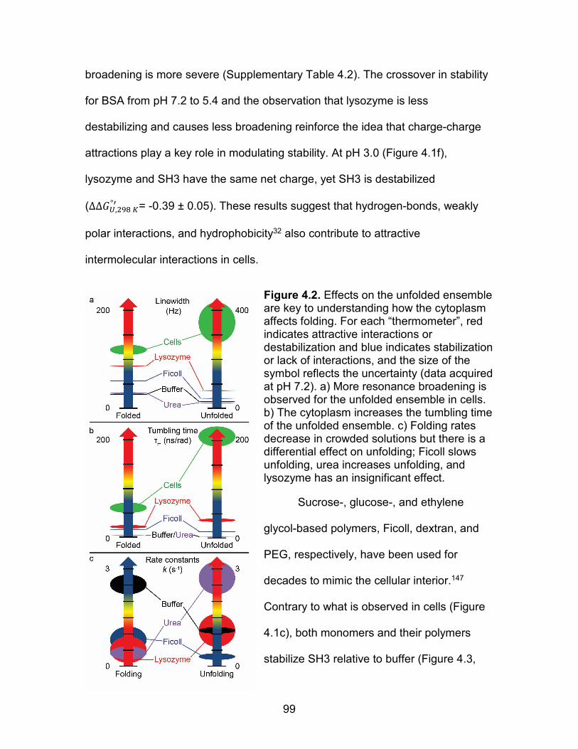
99

broadening is more severe (Supplementary Table 4.2). The crossover in stability

for BSA from pH 7.2 to 5.4 and the observation that lysozyme is less

destabilizing and causes less broadening reinforce the idea that charge-charge

attractions play a key role in modulating stability. At pH 3.0 (Figure 4.1f),

lysozyme and SH3 have the same net charge, yet SH3 is destabilized

(ΔΔ��,HIJ K° = -0.39 ± 0.05). These results suggest that hydrogen-bonds, weakly

polar interactions, and hydrophobicity32 also contribute to attractive

intermolecular interactions in cells.

Figure 4.2. Effects on the unfolded ensemble are key to understanding how the cytoplasm affects folding. For each “thermometer”, red indicates attractive interactions or destabilization and blue indicates stabilization or lack of interactions, and the size of the symbol reflects the uncertainty (data acquired at pH 7.2). a) More resonance broadening is observed for the unfolded ensemble in cells. b) The cytoplasm increases the tumbling time of the unfolded ensemble. c) Folding rates decrease in crowded solutions but there is a differential effect on unfolding; Ficoll slows unfolding, urea increases unfolding, and lysozyme has an insignificant effect.

Sucrose-, glucose-, and ethylene

glycol-based polymers, Ficoll, dextran, and

PEG, respectively, have been used for

decades to mimic the cellular interior.147

Contrary to what is observed in cells (Figure

4.1c), both monomers and their polymers

stabilize SH3 relative to buffer (Figure 4.3,

100

Supplementary Tables 4.1-4.3). Furthermore, the monomers are more stabilizing

than the polymers; the opposite of what is usually implied by the term

macromolecular crowding. In addition, theory predicts the stabilization arises

from entropic effects, yet ethylene glycol and PEG stabilize SH3 enthalpically,

while the sugar-induced stabilization is entropic. Clearly, synthetic polymers are

poor mimics of the cellular interior.

Surprisingly, urea is the most accurate mimic of the thermodynamics

observed in cells (Figure 4.1c). This cosolute destabilizes proteins by interacting

favorably with the backbone,155 which is more exposed in the unfolded

ensemble.154 Urea shows a strong enthalpic destabilization that overcomes a

stabilizing entropic term at 298 K (ΔΔ��°= -1.32 ± 0.07, ΔΔ��°= -3 ± 1, TΔΔ��°= -2

± 1 kcal/mol at 100 g/L). This is the same pattern seen in cells. These data

strengthen our conclusion that the destabilization arises by attractive interactions

with the unfolded ensemble.

Resonance broadening (Figure 4.2a) is only an approximate measure of

attractive intermolecular interactions. Attractive interactions with larger proteins

slow tumbling. Therefore, to obtain more detailed knowledge, we used 19F

relaxation to estimate tumbling times (τm) of SH3.150 In buffer, τm is 4 ns for the

folded state and 3 ns for the unfolded ensemble (Figure 4.3b, Supplementary

Table 4.4), similar to published values.156 In cells, the τm increases to 60 ns for

the folded state and 210 ns for the unfolded ensemble, 15- and 70-fold

increases, respectively. Increases may arise from higher viscosity (η), but the

viscosity in cells is only about twice that in water.150 The larger effect on the

101

unfolded ensemble bolsters our conclusion that the interior of the cell interacts

more strongly with the unfolded ensemble, which explains the observed

destabilization.

Figure 4.3. Synthetic polymers do not replicate the cytoplasm. Buffer (black) and in-cell (red) curves are reproduced from Figure 4.1c. Error bars for the 298 K data are the standard deviation of three independent trials at 298 K. a) Glucose and 20 kDa dextran, b) sucrose and 70 kDa Ficoll (all at 300 g/L), c) ethylene glycol, 8 kDa PEG and 35 kDa PEG (all at 200 g/L) stabilize the SH3 domain.

To lend further support to our conclusion,

we examined the effects of Ficoll and lysozyme on

τm. Ficoll increased τm to 15 ns and 13 ns for the

folded state and unfolded ensemble, respectively.

These increases likely arise from the large

increase in viscosity.42 The viscosity of the 100 g/L

lysozyme solution is only 1.3 times that of water,42

yet the apparent τm increased to 21 ns for the

folded state and 37 ns for the unfolded ensemble.

These data strongly support the idea that effects

on the unfolded ensemble are the cause of the stability decrease in cells.

We also quantified the effects of cosolutes on folding and unfolding rates.

We were unable to asses the rates in cells because, although SH3 is stable for

one hour in cells, it is degraded during the >12 h needed for these experiments

(all other in-cell experiments require a few minutes). Rate data were acquired in

102

lysozyme, urea and Ficoll (Figure 4.3c, Supplementary Table 4.5). Ficoll (70 kDa,

300 g/L) decreased the folding rate 2.5-fold, but decreased the unfolding rate

2.8-fold. The slower folding is consistent with the viscosity increase and slower

unfolding consistent with both viscosity and the idea of an entropic pressure for

the protein to adopt a compact form.157,158 In contrast, lysozyme (100 g/L) slowed

folding 5-fold, but had no effect on unfolding. Like lysozyme, urea (100 g/L)

slowed folding 5-fold, but increased unfolding only 2.5 fold. We speculate that

urea’s small size allows it to penetrate the folded state to speed unfolding and its

interaction with the backbone in the unfolded ensemble slowed folding, whereas

lysozyme is too large to affect unfolding, but slows folding via interactions with

the unfolded ensemble. These observations reinforce the idea that biologically

relevant conditions can destabilize proteins by facilitating favorably interactions

with the unfolded ensemble.

In summary, physiologically relevant information about proteins exteriors

have been hidden because proteins are most often studied in buffer instead of in

cells. This limitation does not matter for protein cores; they yield relevant

information even in buffer because interior atoms experience the same

environment in cells as they do in buffer -- they are surrounded by other protein

atoms. Exteriors, however, are fundamentally different. In buffer, the surface is

exposed to mostly water, but the cytoplasm is dramatically complex and

crowded. Our data indicate that the cellular matrix interacts strongly with protein

surfaces, and these interactions affect both the equilibrium thermodynamics and

kinetics of folding. Although synthetic polymers are important in industrial

103

applications, these cosolutes are poor models of the cellular interior. These data

also show that theories to explain protein behavior in cells must consider both the

folded state and unfolded ensemble and must include terms for both hard-core

repulsions and charge-charge interactions, but also hydrogen bonds, weakly

polar interactions and hydrophobics. Recent modifications to theory,159 as well as

simulations of intracellular dynamics are pointing the way.73 Most importantly, our

data show that studying protein folding in living cells is key to gaining information

needed to understand the role of proteins in biology.

Methods

Protein expression for in-cell NMR

Plasmids harboring the gene encoding the N-terminal SH3 domain of drk

(SH3) were transformed into Agilent BL21 DE3 Gold cells by heat-shock. A

single colony was used to inoculate a 5 mL culture of Lennox broth (LB, 10 g/L

tryptone, 5 g/L yeast extract, 5 g/L NaCl) supplemented with 100 μg/mL

ampicillin. The culture was incubated with shaking at 37 °C (New Brunswick

Scientific Innova I26, 225 rpm). After 8 h, 50 μL of the saturated culture was used

to inoculate 50 mL of supplemented M9 media (50 mM Na2HPO4, 20 mM

KH2PO4, 9 mM NaCl, 4 g/L glucose, 1 g/L NH4Cl, 0.1 mM CaCl2, 2 mM MgSO4,

10 mg/L thiamine, 10 mg/L biotin, and 150 mg/L ampicillin, pH 7.4).

The 50 mL culture was shaken at 37 °C overnight. The culture was then

diluted to 100 mL with supplemented M9 media. 5-Fluoroindole (in

dimethylsulfoxide) was added to a final concentration of 0.1 g/L, and the culture

104

was shaken for 30 min. Isopropyl β-D-1-thiogalactopyranoside (IPTG, 1 mM final

concentration) was used to induce expression. After 45 min, cells were pelleted

at 1000g and resuspended in M9 media without 5-fluoroindole, and expression

was again induced to ensure efficient incorporation of the label. After 45 min, the

cells were pelleted at 1000g and washed three times with in-cell NMR buffer (200

mM HEPES, 100 mM bis-tris propane, 50 μg/mL chloramphenicol, 150 μg/mL

ampicillin, pH ~7.6. Chloramphenicol was used to halt protein expression prior to

NMR. Cell pellets were resuspended in 300 μL of in-cell NMR buffer and loaded

into a standard 5 mm NMR tube. Typical cell slurries were 50% wet cells by

volume.

Protein expression for purification

Transformation and growth were performed as described in the first

paragraph of the previous section.

The 50 mL cultures were shaken at 37 °C overnight, diluted to 1 L with

supplemented M9 media and shaken until the optical density at 600 nm reached

0.6. 5-Fluoroindole was added (0.1 g/L final concentration) and the culture

shaken for an additional 30 min. IPTG (1 mM final concentration) was used to

induce expression. After 1 h, cells were pelleted at 1000g at 10 oC for 30 min,

resuspended in 50 mM Tris-HCl (pH 7.5) and frozen at -80 °C.

Protease inhibitors (Sigma-Aldrich P-2714, containing AEBSF, aprotinin,

bestatin, E-64, EDTA and leupeptin, refer to Methods Chapter 2 for

concentrations) were added before lysis. Cells were lysed by sonication (Fisher

105

Scientific Sonic Dismembrator Model 500, 15% amplitude, 15 min, 67% duty

cycle) on ice. Cell debris was removed by centrifugation at 16000g at 10 oC for

30 min, and the sample was passed through a 0.45 μm filter. Purification involved

two chromatography steps using a GE AKTA FPLC. The first step was anion

exchange (20 mL GE Q column, 5-45% gradient over 4 column volumes, 50 mM

Tris-HCl wash buffer, 50 mM Tris-HCl/1 M NaCl eluant buffer, pH 7.5). SH3 binds

weakly to anion exchange media. Protease inhibitors were added to the SH3-

containing fractions, and the sample was passed through a 0.22 μm filter. The

second step was size exclusion chromatography (GE Superdex 75 column eluted

with 50 mM K2HPO4, 150 mM NaCl, 1 mM EDTA, pH 7.2, 0.5 ml/min flow rate).

Purified protein was dialyzed against 4 L, 17 MΩ cm-1 H2O for 4 h at room

temperature and/or overnight at 5 °C. Buffer was changed every 1.5 to 2 h. After

dialysis and filtration through a 0.22 μm filter, the sample was flash frozen in a

dry-ice/ethanol bath and lyophilized for 12 h (Labconco FreeZone). Purity was

asses via SDS-PAGE.

NMR

In-cell samples were prepared as described above. For in vitro

experiments, purified 19F-labeled protein was added to NMR buffer (50 mM acetic

acid/sodium acetate, HEPES, bis-tris propane, pH 7.2). One experiment used

NMR buffer plus 150 mM NaCl, to assess salt dependence. 19F-spectra were

acquired at 4 °C (5 °C for in-cell experiments), 10 °C, 15 °C, 20 °C, 25 °C, 30 °C,

35 °C, 40 °C, and 45 °C with a Bruker Avance III HD spectrometer operating at a

19F Larmor frequency of 470 MHz running Topspin Version 3.2 and equipped

106

with a Bruker QCI cryoprobe. The temperature was calibrated with a two point

standard curve using deuterated methanol. The total relaxation delay for one-

dimensional experiments was 5 s. The sweep width was 70 ppm. The number of

scans depended on cosolute and ranged from 32 to 256.

Carr-Purcell-Meiboom-Gill (CPMG)-based spin-spin relaxation time (T2)

measurements used mixing times (tmix) of 1.0, 2.1,4.2, 6.3, 8.4, 16.8, 33.5, and

67.0 ms. A 955 Hz effective field was used to negate effects of chemical

exchange. The transmitter was placed on-resonance to prevent ineffective

refocusing. Spin-lattice relaxation times (T1) were measured using an inversion

recovery sequence (tmix: 0, 0.05, 0.10, 0.25, 0.50, 0.80, 1.00 and 1.50 s). A

Bruker library NOESY experiment (tmix: 1.5, 50, 90, 150, 225, 300, 600 and 1000

ms for buffer and 1.5, 70, 140, 210, 300, 500, and 800 ms for crowded samples)

with a 2 s relaxation delay was used to measure folding/unfolding rates. Sweep

widths were 70 ppm in both dimensions. 1024 complex points were collected

during t2 with 64 complex points in t1 at each tmix. Sixteen transients were

acquired per increment.

The SH3 domain is degraded in cells in a few hours, but T1 and T2

measurements require ~5 h. Therefore, T2 measured in cells used a 0.002 s

constant time period and a 1000 Hz effective field.

19F-spectra were acquired before and after the relaxation and exchange

experiments to assess sample integrity and reversibility. Populations of the

folded and unfolded states remained constant, or the dataset was discarded. For

107

the in-cell samples, the cell slurry was removed after the experiment and gently

pelleted. The supernatant was diluted two-fold. The cells were resuspended in

0.4 mL of in-cell NMR buffer plus protease inhibitors, lysed by sonication and

clarified at 16000g. 19F spectra were acquired on the supernatant to assess

protein leakage and on the lysates to assess the effect of lysates on stability. No

leakage was observed. A labeled metabolite that leaks from the cells overlaps

with the peak corresponding to the unfolded ensemble. Integrals from the 19F

spectrum of the supernatant were subtracted from the in-cell integrals.

Resonances were referenced to trifluoroacetic acid (0.1%) in D2O placed

in a coaxial insert inside the NMR tube. The D2O also served to lock the

spectrometer.

Data processing

Data were processed with Topspin 3.2. For temperature variation

experiments, free induction decays (fids, 50k points each) were subjected to a 10

to 15 Hz broadening function before zero filling (to 131,000 points) and Fourier

transformation. For T1 and T2 experiments, fids (50k points) were subjected to a

10- to 15-Hz broadening function before zero-filling to 131k points. For exchange

spectroscopy, t2 data (1024 complex points) were subjected to a cosine squared

bell function before zero filling to 4096 points. t1 data were linear predicted to 256

points before application of a cosine squared bell function. Subsequent zero

filling to 512 points and Fourier transform yielded the final spectra.

108

Resonance intensities were extracted for relaxation experiments. For

temperature variation experiments, peaks were integrated. Peak volumes were

fitted as described. Published assignments were used.149

19F T1 (1/R1) and T2 (1/R2) data were fit using Model Free formalism to

calculate rotational correlation times (τm).160,161 The internal correlation time (τe)

and the order parameter (S2) were set to 20 ps and 0.82 for the folded state and

1200 ps and 0.34 for the unfolded state.156 Chemical shift anisotropy and

asymmetry terms were set to -93.5 ppm and 0.24.162 No μs-ms motion was

observed in buffer, and a 950 Hz effective field was used for the R2

measurements. Therefore, chemical exchange was not included in fitting. The

average 19F-1H distances (r) and τm were then minimized based on fitting the R1

and R2 data.

Analysis of uncertainties

Triplicate datasets, using three different batches of purified protein, were

acquired for the pH 7.2 buffer dataset. The sample standard deviations

depended on temperature (±52 cal/mol, ±45 cal/mol, ±59 cal/mol, ±31 cal/mol,

±31 cal/mol, ±66 cal/mol, ±61 cal/mol, ±14 cal/mol, ±35 cal/mol at 4 °C, 10 °C, 15

°C, 20 °C, 25 °C, 30 °C, 35 °C, 40 °C, and 45 °C, respectively). For buffer, we

used these standard deviations to drive Monte Carlo error analysis. One-

thousand randomly-generated datasets were fitted to the integrated Gibbs-

Helmholtz equation at Tref (Appendix 2). To extrapolate ∆��,MNOP° and ∆��,MNOP

° , and

their uncertainties, to 298 K, the average and sample standard deviations of

109

∆��,MNOP° , Tref and ∆��,�° from this analysis were used to drive another Monte Carlo

analysis (N=106) using Kirchoff’s relations (Appendix 3). The uncertainties in

∆��,HIJ K° and ∆��,HIJ K° are larger than the uncertainty in ∆��,HIJ K° because the

enthalpy and entropy changes are derived from for three variables (∆��,MNOP° , Tref

and ∆��,�° ) and their uncertainties.

For the in-cell data, a similar method was used. Triplicate data were

obtained for the 10 °C, 25 °C and 40 °C datasets. For the other datasets

uncertainties from the nearest-neighbor triplicate dataset were used to drive the

analysis. For example, the 5 °C and 15 °C used the uncertainty associated with

the 10 °C dataset.

For in-vitro experiments in the presence of crowders, triplicate 25 °C data

were acquired on the same sample. This uncertainty was scaled as described in

the first paragraph of this section and used to drive the Monte Carlo analysis.

For in vitro relaxation-rates, one mixing time was acquired three times.

The sample standard deviation was used to drive Monte Carlo analysis (N=1000)

to obtain R1 and R2 (Appendix 4, 5). The mean and standard deviations from this

analysis were used to drive another Monte Carlo (N=1000) using the Model Free

approach to obtain r, τm and their uncertainties (Appendix 6). Fitted r values

varied from 1.8 to 2.1 Å for the folded state and 2.0 to 2.4 Å for the unfolded

state. For fitting in-cell R2, r was varied between these ranges, and τm was then

fitted using only R2. The uncertainty in τm is the range of values from these fits.

110

Folding rate data in buffer were acquired in triplicate and fitted as

described (Appendix 7).163 The uncertainty is the sample standard deviation. For

in vitro folding-rates, one mixing time was acquired three times. The sample

standard deviation was used to drive Monte Carlo analysis (N=100). For folding

rates, R1 was fixed to the value acquired from inversion recovery experiments for

in vitro crowded conditions.

In-cell pH

Purified protein was resuspended in 50 mM citrate, 50 mM bis-tris

propane, 50 mM HEPES, 50 mM borate, 5% D2O, 0.1% DSS (pH values: 5.0,

5.8, 6.5, 6.9, and 7.5). Data were acquired from 10 to 40 °C in 5 °C increments.

The difference in the 19F chemical shifts between the two states is sensitive to pH

(Supplementary Figure 4.1). These experiments were combined with two NMR

buffer experiments [50 mM acetate, 50 mM HEPES, 50 mM bis-tris at pH 7.2

(with and without 0.15 M NaCl)] to assess salt effects, which were minimal. Shift

change as a function pH was fitted to a second order polynomial to produce a

standard curve. Shift differences from in-cell data sets were then compared to

this standard curve to obtain the pH in cells. The values in cells, pH 7.2, compare

favorably to the external meter reading minus 0.4 pH units, as previously

described by us and others.5,54

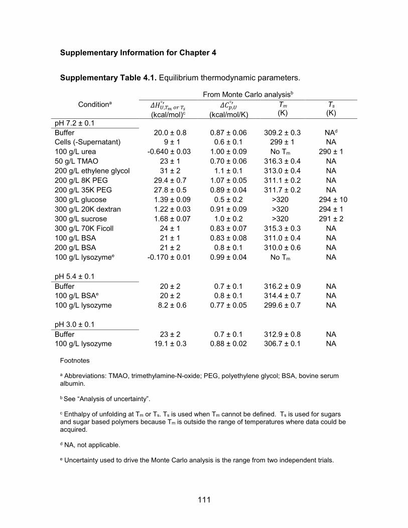
111

Supplementary Information for Chapter 4

Supplementary Table 4.1. Equilibrium thermodynamic parameters.

From Monte Carlo analysisb Conditiona Q��,MR �@ MS

° (kcal/mol)c

Q��,�° (kcal/mol/K)

Tm (K)

Ts (K)

pH 7.2 ± 0.1 Buffer 20.0 ± 0.8 0.87 ± 0.06 309.2 ± 0.3 NAd Cells (-Supernatant) 9 ± 1 0.6 ± 0.1 299 ± 1 NA 100 g/L urea -0.640 ± 0.03 1.00 ± 0.09 No Tm 290 ± 1 50 g/L TMAO 23 ± 1 0.70 ± 0.06 316.3 ± 0.4 NA 200 g/L ethylene glycol 31 ± 2 1.1 ± 0.1 313.0 ± 0.4 NA 200 g/L 8K PEG 29.4 ± 0.7 1.07 ± 0.05 311.1 ± 0.2 NA 200 g/L 35K PEG 27.8 ± 0.5 0.89 ± 0.04 311.7 ± 0.2 NA 300 g/L glucose 1.39 ± 0.09 0.5 ± 0.2 >320 294 ± 10 300 g/L 20K dextran 1.22 ± 0.03 0.91 ± 0.09 >320 294 ± 1 300 g/L sucrose 1.68 ± 0.07 1.0 ± 0.2 >320 291 ± 2 300 g/L 70K Ficoll 24 ± 1 0.83 ± 0.07 315.3 ± 0.3 NA 100 g/L BSA 21 ± 1 0.83 ± 0.08 311.0 ± 0.4 NA 200 g/L BSA 21 ± 2 0.8 ± 0.1 310.0 ± 0.6 NA 100 g/L lysozymee -0.170 ± 0.01 0.99 ± 0.04 No Tm NA pH 5.4 ± 0.1 Buffer 20 ± 2 0.7 ± 0.1 316.2 ± 0.9 NA 100 g/L BSAe 20 ± 2 0.8 ± 0.1 314.4 ± 0.7 NA 100 g/L lysozyme 8.2 ± 0.6 0.77 ± 0.05 299.6 ± 0.7 NA pH 3.0 ± 0.1 Buffer 23 ± 2 0.7 ± 0.1 312.9 ± 0.8 NA 100 g/L lysozyme 19.1 ± 0.3 0.88 ± 0.02 306.7 ± 0.1 NA

Footnotes a Abbreviations: TMAO, trimethylamine-N-oxide; PEG, polyethylene glycol; BSA, bovine serum albumin. b See “Analysis of uncertainty”. c Enthalpy of unfolding at Tm or Ts. Ts is used when Tm cannot be defined. Ts is used for sugars and sugar based polymers because Tm is outside the range of temperatures where data could be acquired. d NA, not applicable. e Uncertainty used to drive the Monte Carlo analysis is the range from two independent trials.

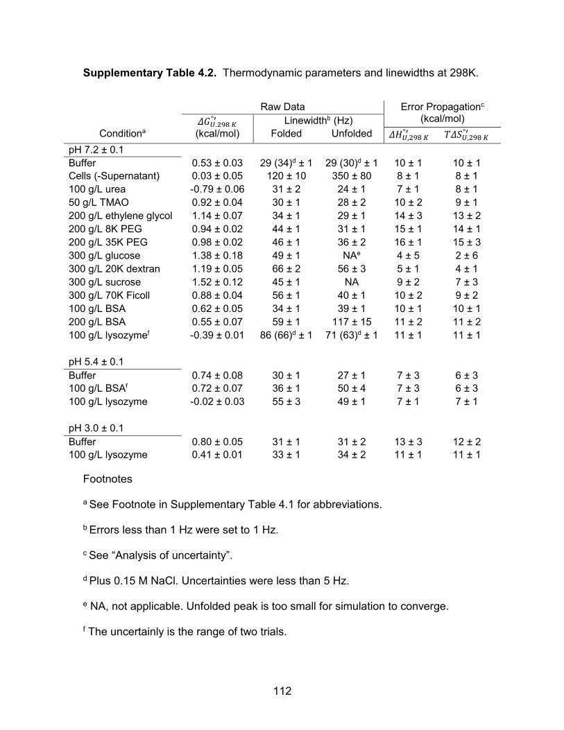
112

Supplementary Table 4.2. Thermodynamic parameters and linewidths at 298K.

Raw Data Error Propagationc (kcal/mol) Q��,HIJ K° Linewidthb (Hz)

Conditiona (kcal/mol) Folded Unfolded Q��,HIJ K° ;Q��,HIJ K°

pH 7.2 ± 0.1 Buffer 0.53 ± 0.03 29 (34)d ± 1 29 (30)d ± 1 10 ± 1 10 ± 1 Cells (-Supernatant) 0.03 ± 0.05 120 ± 10 350 ± 80 8 ± 1 8 ± 1 100 g/L urea -0.79 ± 0.06 31 ± 2 24 ± 1 7 ± 1 8 ± 1 50 g/L TMAO 0.92 ± 0.04 30 ± 1 28 ± 2 10 ± 2 9 ± 1 200 g/L ethylene glycol 1.14 ± 0.07 34 ± 1 29 ± 1 14 ± 3 13 ± 2 200 g/L 8K PEG 0.94 ± 0.02 44 ± 1 31 ± 1 15 ± 1 14 ± 1 200 g/L 35K PEG 0.98 ± 0.02 46 ± 1 36 ± 2 16 ± 1 15 ± 3 300 g/L glucose 1.38 ± 0.18 49 ± 1 NAe 4 ± 5 2 ± 6 300 g/L 20K dextran 1.19 ± 0.05 66 ± 2 56 ± 3 5 ± 1 4 ± 1 300 g/L sucrose 1.52 ± 0.12 45 ± 1 NA 9 ± 2 7 ± 3 300 g/L 70K Ficoll 0.88 ± 0.04 56 ± 1 40 ± 1 10 ± 2 9 ± 2 100 g/L BSA 0.62 ± 0.05 34 ± 1 39 ± 1 10 ± 1 10 ± 1 200 g/L BSA 0.55 ± 0.07 59 ± 1 117 ± 15 11 ± 2 11 ± 2 100 g/L lysozymef -0.39 ± 0.01 86 (66)d ± 1 71 (63)d ± 1 11 ± 1 11 ± 1

pH 5.4 ± 0.1 Buffer 0.74 ± 0.08 30 ± 1 27 ± 1 7 ± 3 6 ± 3 100 g/L BSAf 0.72 ± 0.07 36 ± 1 50 ± 4 7 ± 3 6 ± 3

100 g/L lysozyme -0.02 ± 0.03 55 ± 3 49 ± 1 7 ± 1 7 ± 1

pH 3.0 ± 0.1 Buffer 0.80 ± 0.05 31 ± 1 31 ± 2 13 ± 3 12 ± 2 100 g/L lysozyme 0.41 ± 0.01 33 ± 1 34 ± 2 11 ± 1 11 ± 1

Footnotes a See Footnote in Supplementary Table 4.1 for abbreviations. b Errors less than 1 Hz were set to 1 Hz. c See “Analysis of uncertainty”. d Plus 0.15 M NaCl. Uncertainties were less than 5 Hz. e NA, not applicable. Unfolded peak is too small for simulation to converge. f The uncertainly is the range of two trials.

113

Supplementary Table 4.3. Change in thermodynamic parameters at 298 K.

Green shading indicates significant stabilization (i.e., >0 uncertainty). Red

shading indicates significant destabilization. For other entries, the uncertainties

are too large to permit classification.

Conditiona

QQ��,HIJ K° (kcal/mol)

QQ��,HIJ K° (kcal/mol)

;QQ��,HIJ K° (kcal/mol)

pH 7.2 ± 0.1 Cells (- Supernatant) -0.50 ± 0.06 -2 ± 1 -2 ± 1 100 g/L urea -1.32 ± 0.07 -3 ± 1 -2 ± 1 50 g/L TMAO 0.39 ± 0.05 0 ± 2 -1 ± 1 200 g/L ethylene glycol 0.61 ± 0.08 4 ± 3 3 ± 2 200 g/L 8K PEG 0.41 ± 0.04 5 ± 1 4 ± 1 200 g/L 35K PEG 0.45 ± 0.04 6 ± 1 5 ± 3 300 g/L glucose 0.85 ± 0.18 -6 ± 5 -8 ± 6 300 g/L 20K dextran 0.66 ± 0.06 -5 ± 1 -6 ± 1 300 g/L sucrose 0.99 ± 0.12 -1 ± 2 -3 ± 3 300 g/L 70K Ficoll 0.35 ± 0.05 0 ± 2 -1 ± 2 100 g/L BSA 0.09 ± 0.06 0 ± 1 0 ± 1 100 g/L lysozymeb -0.92 ± 0.03 1 ± 1 1 ± 1

pH 5.4 ± 0.1 100 g/L BSAb -0.02 ± 0.11 0 ± 3 0 ± 4 100 g/L lysozyme -0.76 ± 0.09 0 ± 3 1 ± 3

pH 3.0 ± 0.1 100 g/L lysozyme -0.39 ± 0.05 -2 ± 3 -1 ± 2

Footnotes a See Footnote in Supplementary Table 4.1 for abbreviations. b The uncertainly is the range of two trials.

Supplementary Table 4.4. Relaxation rates and correlation times (298 K, pH 7.2 ± 0.1).

Folded Unfolded Conditiona R1 (s-1) R2 (s-1) r (Å) τm (ns) R1 (s-1) R2 (s-1) r (Å) τm (ns)

Buffer 2.5 ± 0.1 30 ± 2 1.93 ± 0.02 3.9 ± 0.2 2.0 ± 0.2 13.6 ± 0.3 2.09 ± 0.07 2.9 ± 0.2 Cells NAb 440 set 60 ± 10 NA 560 set 210 ± 20 300 g/L 70K Ficoll 1.53 ± 0.09 113 ± 4 1.93 ± 0.02 15.3 ± 0.5 1.4 ± 0.2 42 ± 2 2.2 ± 0.1 13.4 ± 0.8 100 g/L urea 1.8 ± 0.2 28 ± 2 2.06 ± 0.05 4.0 ± 0.3 1.49 ± 0.06 11.3 ± 0.1 2.34 ± 0.04 2.5 ± 0.1 100 g/L lysozyme 1.46 ± 0.08 165 ± 27 1.86 ± 0.04 21 ± 3 1.37 ± 0.05 110 ± 8 2.10 ± 0.02 37 ± 3

Footnotes a See “Analysis of uncertainty”. The cellular viscosity is thought to be 2-4 times that of water.150 300 g/L Ficoll is ~24 times water and 100 g/L lysozyme is ~1.3 times water.42 b NA, not applicable. R1 could not be obtained in cells due to degradation.

11

4

115

Supplementary Table 4.5. Folding rates (s-1) at 298 K, pH 7.2 ± 0.1.

Conditiona kf ku

Buffer 2.5 ± 0.3 1.1 ± 0.1 300 g/L 70K 0.8 ± 0.4 0.3 ± 0.1 100 g/L urea 0.4 ± 0.2 2.7 ± 0.5 100 g/L 0.5 ± 0.4 1.1 ± 0.5

Footnotes

aSee “Analysis of uncertainty”.

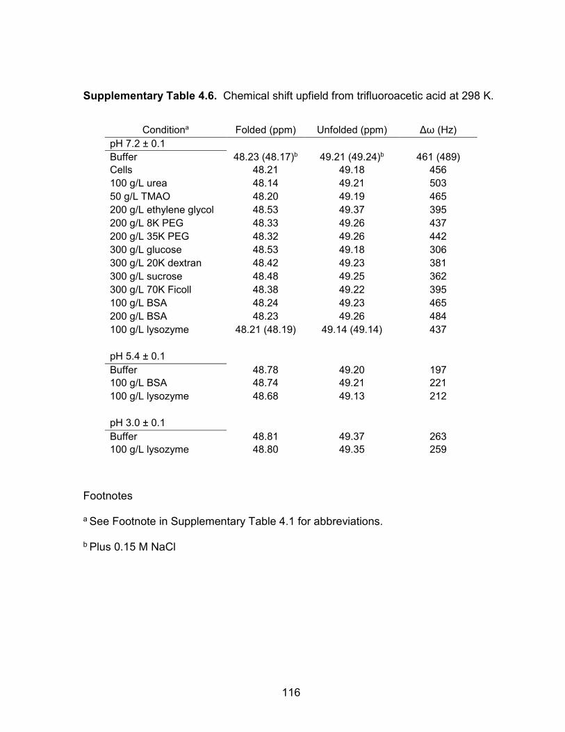
116

Supplementary Table 4.6. Chemical shift upfield from trifluoroacetic acid at 298 K.

Conditiona Folded (ppm) Unfolded (ppm) Δω (Hz) pH 7.2 ± 0.1 Buffer 48.23 (48.17)b 49.21 (49.24)b 461 (489) Cells 48.21 49.18 456 100 g/L urea 48.14 49.21 503 50 g/L TMAO 48.20 49.19 465 200 g/L ethylene glycol 48.53 49.37 395 200 g/L 8K PEG 48.33 49.26 437 200 g/L 35K PEG 48.32 49.26 442 300 g/L glucose 48.53 49.18 306 300 g/L 20K dextran 48.42 49.23 381 300 g/L sucrose 48.48 49.25 362 300 g/L 70K Ficoll 48.38 49.22 395 100 g/L BSA 48.24 49.23 465 200 g/L BSA 48.23 49.26 484 100 g/L lysozyme 48.21 (48.19) 49.14 (49.14) 437 pH 5.4 ± 0.1 Buffer 48.78 49.20 197 100 g/L BSA 48.74 49.21 221 100 g/L lysozyme 48.68 49.13 212 pH 3.0 ± 0.1 Buffer 48.81 49.37 263 100 g/L lysozyme 48.80 49.35 259

Footnotes a See Footnote in Supplementary Table 4.1 for abbreviations. b Plus 0.15 M NaCl

117

Supplementary Figure 4.1. Chemical shift between the folded and unfolded peaks

(δω) is pH dependent. Black circles, δω in buffer at various pH values (see

Methods). Squares, δω in NMR buffer with (red) and without (blue) 150 mM NaCl.

Data were fitted to a second-order polynomial (δω=-24.77×pH2+449.9×pH-1474).

The 95% confidence interval is shown by the dotted curve. The inset shows 19F

spectra at pH 7.5, 6.5 and 5.8 at 298 K. The spectra were normalized to the position

and intensity of the unfolded ensemble at pH 7.5.

118

APPENDIX 1. INTERLEAVED SOLEXSY PULSE CODE WITH SIGN CODING REMOVED.

;SOLEXSY ;Bruker pp to measure 1H/2H exchange as described in ;Chevelkov, et. al., JBNMR, 2010 ;based on H(CACO)NH ;F1(H) -> F2(Ca) -> F2(C=O) -> F3(N,t1) -> F1(H,t2) ;on/off resonance Ca and C=O pulses using shaped pulse ;phase sensitive (t1) ;phase sensitive using TPPI (t2) ;$CLASS=HighRes ;$DIM=3D ;edits made by Austin E. Smith, UNC Chapel Hill ;Avance-III HD, Topspin 3.2, prosol compliant ;Removed sign coding for proteins with good peak dispersion or short T2 ;INTERLEAVED, set td1 = # in VDLIST prosol relations=<triple> #include <Avance.incl> #include <Grad.incl> #include <Delay.incl> ;; AES Pulse Linkages, just set p21 and p1 ;; unlink if necessary "p22=p21*2" ;;15N 180 links to 90 "p2=p1*2" ;;1H 180 links to 90 "p27=p1" ;;watergate pulses "p0=p1" ;;watergate final pulse "p19=800u" ;;purge grad in mix ;;AES linkages for 15N incrementation "in0=(inf2/4)/(1+cnst0)" "in29=(in0*cnst0)" "in30=(in0*cnst0)" "cnst5=d30/in30" ;; Max number of increments "cnst6=d30-(td2*in30)" ;;Time remaining in constant time period ;;Delays "d0=4u" "d4=1/(4*cnst1)" ;;1/(4*JCaH) ~1.8 ms "d11=30m" "d12=20u"

119

"d16=183u" "d21=d4*2" ;; CA-H 2*inept time exact "d22=1/(4*cnst2)" ;;1/(4*JCaCO) ~4.5 ms "d23=1/(4*cnst3)" ;;1/(4*JCON) ~16.7 ms "d24=1/(4*cnst4)" ;;1/(4*JNH) ~2.5ms "d25=d22*2" ;; CA-CO 2*inept time exact "d27=d23-d25" "d29=4u" "d30=d23" "DELTA1=d22-d21-p14-4u" "DELTA2=d22-p14-4u" "DELTA6=d24-p16-d16-p27*3-d19*5" "DELTA7=d19-p22/2" "DELTA8=d24-p16-d16-p27*2-p0-d19*5-4u" define list<delay> exchange=<$VDLIST> ;;Offsets "spoff2=0" ;; p90 on CA to XY "spoff3=0" "spoff5=bf2*((cnst21-cnst22)/1000000)" ;; to move bf2 from CA to CO "spoff8=0" "spoff9=0" "spoff13=bf2*((cnst26-cnst21)/1000000)" ;; move bf2 to midle when on CO "spoff7=-bf2*((cnst21-cnst22)/1000000)" ;; bf2 on CA from CO aqseq 312 1 d11 ze d11 LOCKDEC_ON d11 LOCKH_ON d11 H2_PULSE d11 pl17:f4 d11 pl16:f3 2 d11 do:f3 5u pl3:f3 2u pl2:f2 "DELTA=exchange" 3 d11 H2_LOCK 10m LOCKH_OFF d1 pl1:f1 fq=cnst22(bf ppm):f2 50u LOCKH_ON

120

d12 H2_PULSE d11 UNBLKGRAMP d11 (p3 ph11):f2 p19:gp2 d16 ;; Ha to Ca (p1 ph11) d4 (center (p2 ph2) (p14:sp3 ph1):f2 ) d4 (p1 ph2) p16:gp3 d16 ;; transfer from Ca to 15N (p13:sp2 ph12):f2 ;; CA p90 to Y d21 pl19:f1 DELTA1 cpds1:f1 ph2 (p14:sp5 ph1):f2 ;; CO p180 of res. 4u (p24:sp9 ph4):f2 ;; CA p180 on res. DELTA2 (p14:sp5 ph1):f2 ;; CO p180 of res. refocuss 4u (p13:sp8 ph1):f2 ;; CA p90 15u fq=cnst21(bf ppm):f2 ;; CO chemshift 15u (p13:sp2 ph13):f2 ;; CO p90 4u (p14:sp7 ph1):f2 ;; CA p180 refocus d25 ;; CA-CO transfer d27 ;; CA-CO transfer (center (p14:sp3 ph1):f2 (p22 ph1):f3 ) d27 d22 (p14:sp7 ph1):f2 ;; CA p180 of res. d22 (p13:sp8 ph3):f2 ;; CO p90 to Z 4u do:f1 ;; t1 encode using semiconstant time evolution

121

4u cpds4:f4 (p21 ph5):f3 ;; N p90 to Y: COzNy 4u d30 pl1:f1 ;; td - kappa*t1/2 (center (p14:sp3 ph1):f2 (p22 ph1):f3 ) 4u d23 ;; td (center (p14:sp7 ph1):f2 (p2 ph10):f1 ) ;; CA p180 refocus d29 ;; kappa*t1/2 d0 ;; t1/2 (center (p8:sp13 ph4):f2 (p2 ph1):f1 ) d0 ;; t1/2 (p22 ph1):f3 4u (center (p8:sp13 ph4):f2 (p2 ph1):f1 ) 4u (center (p14:sp7 ph1):f2 (p2 ph10):f1 ) 4u (p21 ph18):f3 ;; 15N to Z from Nx 4u do:f4 ;; EXCHANGE (tmix) DELTA (p1 ph1):f1 ;; H2O saturation/purge 4u p19:gp3 d16 ;; Rev INEPT (p21 ph15):f3 ;; 15N to Y for Inept d24 (center (p2 ph1) (p22 ph1):f3 ) d24 (p21 ph2):f3 ;; 15N along Z 4u p16:gp3 d16 ;; WATERGATE (p1 ph2) DELTA6 ;;;; d24-p16-d16-p27*3-d19*5

122

p16:gp4 d16 pl18:f1 p27*0.231 ph16 d19*2 p27*0.692 ph16 d19*2 p27*1.462 ph16 DELTA7 ;;d19-p22 (p22 ph1):f3 DELTA7 p27*1.462 ph17 d19*2 p27*0.692 ph17 d19*2 p0*0.231 ph17 4u p16:gp4 d16 DELTA8 ;; d24-p16-d16-p27*2-p0-d19*5-4u 4u pl16:f3 BLKGRAMP go=2 ph31 cpd3:f3 20u do:f3 10m wr #0 if #0 zd 20u exchange.inc lo to 2 times td1 20u exchange.res 20u ip18 20u dd30 20u id29 20u id0 lo to 2 times td2 d11 d11 H2_LOCK d11 LOCKH_OFF d11 LOCKDEC_OFF exit ph1=0 ph2=1 ph3=0 ph4=0

123

ph5=0 ph10=2 ph15=0 2 ;; 15N to Y for t1 and HN inept ph11=0 0 2 2 ;; 1H excite ph12=0 0 0 0 2 2 2 2 ;; CA to Y before d21 - HzCAy refocusing ph13=0 0 0 0 0 0 0 0 2 2 2 2 2 2 2 2 ;; CO to Y before d25 - CAzCOy refocusing ph16=2 ;; in wg 1st cycle ph17=0 ;; in wg 2nd cycle ph18=1 ;; for tppi p90 on 15N after t1 ph31=0 2 2 0 2 0 0 2 2 0 0 2 0 2 2 0 ;pl1 : 1H, f1 hard pulse (default) ;pl2 : 13C, f2 hard pulse (default) ;pl3 : 15N, f3 hard pulse (default) ;pl16: 15N, CPD/BB decoupling ;pl17: 2H, CPD/BB decoupling ;pl19: 1H, f1 DIPSI for CPD/BB decoupling ;sp2 : 13C, f2 sel. p90=p13, on resonance ;sp3 : 13C, f2 sel. p180=p14, on resonance ;sp7 : 13C, f2 sel. p180=p14, for CA when its off resonance. ;sp5 : 13C, f2 sel. p180=p14, for C=O when its off resonance. ;sp8 : 13C, f2 sel. p90=p13, on resonance, time reversed CA ; sp8 for time reversed Calpha pulses ;sp9 : 13C, f2 sel. p180=p24, on CA, CO and CB off resonance, ; sp9 requires higher selectivity than sp3 (Ca only) ;sp13: 13C, f2 sel. p180, on Ca and C=O, adiabatic ;p0 : last p90 in Watergate ;p1 : 1H p90 degree high power ;p2 : 1H p180 degree high power ;p3 : 13C hard p90 for refocusing in beginning ;p8 : 13C sp180 Ca & CO, adiabatic for N Jdecoupling ;p13: f2 channel - 90 degree shaped pulse ;p14: f2 channel - 180 degree shaped pulse ;p16: homospoil/gradient pulse [1 msec] ;p19: short gradient ;p21: 15N p90 degree high power pulse ;p22: 15N p180 degree high power pulse ;p24: f2 channel - 180 degree shaped pulse (sp9) ;p27: Watergate 1H p90 pulse ;p28: weak H2O saturation pulse

124

;d0 : incremented delay (F1 in 2D) [3 usec] ;d1 : relaxation delay; 1-5 * T1 ;d11: delay for disk I/O [30 msec] ;d12: delay for power switching ;d16: delay for homospoil/gradient recovery ;d19: delay for binomial water suppression d19 = (1/(2*d)), d = distance of next null (in Hz) ;DELTA : 1H exchange delay ;d4 : CA-H inept time ;d21: CA-H 2*inept time exact ;d22: CA-CO inept time ;d23: CO-N inept ;d24: N-H inept ;d25: CA-CO 2*inept time exact ;cnst0: kappa in Chevelkov, et al. (0.235) ;cnst1: JCaH (~140 Hz) OPT ;cnst2: JCaCO (~55 Hz) OPT ;cnst3: JCON (~15 Hz) OPT ;cnst4: JNH (~95 Hz) OPT ;cnst5: Max Increments!! ;cnst6: Time remaining for last increment of d30 ;cnst21: CO chemical shift (offset, in ppm) (~180 ppm) ;cnst22: Calpha chemical shift (offset, in ppm) (~55 ppm) ;cnst26: Call chemical shift (offset, in ppm) (~100 ppm) ;o2p: Calpha chemical shift (cnst22) ;NS: 8 * n ;DS: >32 ;td1: number of delays ;td2: number of 15N increments ;FnMODE: TPPI in F2 ;FnMODE: echo-antiecho in F3 (DQD) ;cpds1: decoupling according to sequence defined by cpdprg1 ;cpd2: decoupling according to sequence defined by cpdprg2 ;pcpd1: f1 channel - 90 degree pulse for decoupling sequence ;pcpd2: f2 channel - 90 degree pulse for decoupling sequence ;for z-only gradients: ;gpz2: 60.1% 13C def. in beginning ;gpz3: 40% ;gpz4: 60% ;use gradient files: ;gpnam2: SINE.100 ;gpnam3: SINE.100

125

;gpnam4: SINE.100 ;$Id: hcacongp3d,v 1.4 2007/04/11 13:34:29 ber Exp $

126

APPENDIX 2. MONTE CARLO FOR FITTING IN-CELL DATA TO THE INTEGRATED FORM OF THE GIBBS-HELMHOLTZ EQUATION.

clear all close all tempfull = [277.15;283.15;288.15;293.15;298.15;303.15;308.15;313.15;318.15]; tempIC =[278.15;283.15;288.15;293.15;298.15;303.15;308.15;313.15]; nsamples = 1000; %number of simulations fileID = fopen('CellDataTg.dat','w'); %naming the data file formatSpec = '%d %d %d\n'; %this defines the format of the data file %DATA %Buffer:50 mM acetate, bis-tris propane, HEPES DILUTE = [568;713;690;668;532;340;78;-265;-705]; %Average of all 5-45 DILERR = [30;26;34;18;18;38;35;8;20]; % These are the standard deviation of the mean Raw = [175;359;103;192;29;-151;-276;-604]; % Insert Raw data here Err = [NaN;84;NaN;NaN;52;NaN;NaN;74]; %STD Covar = [84^2 84^2 84^2 52^2 52^2 52^2 74^2 74^2]; %if NaN, used the closest triplicate data. Covar is STD^2 MC = mvnrnd(Raw,Covar,nsamples); % Uses covariance... square the STD std(MC) % You can use this as a check to make sure the sigma generated by the MC is correct %FIT DATA Ts = fittype('dH+dCp*((x-Ts)-(x*log(x/Ts)))','independent',{'x'},'coefficients',{'dH','dCp','Ts'}); % Declaring the fit: a is dH (1000), b is dCp (900), t is Ts (290) TsCp = fittype('dH+920*((x-Ts)-(x*log(x/Ts)))','independent',{'x'},'coefficients',{'dH','Ts'}); % Holding dCp constant Tg = fittype('dH-(T*(dH/Tg))+dCp*(T-(Tg)-(T*log(T/(Tg))))','independent',{'T'},'coefficients',{'dH','dCp','Tg'}); % Declaring the fit: a is dH (20000), b is dCp (900), t is Ts (50) [fit1,gof1] = fit(tempfull,DILUTE,Tg,'startpoint',[20000,900,300],'algorithm','Trust-Region','Robust','on'); % This does the fitting [fit2,gof2] = fit(tempIC,Raw,Tg,'startpoint',[20000,900,300],'algorithm','Trust-Region','Robust','on'); for i=[1:nsamples] % This will fit the data for however many simulations you choose DataMC = MC(i,:)'; % This reads the matrix row-by-row [fitx]=fit(tempIC,DataMC,Tg,'startpoint',[fit2.dH,fit2.dCp,fit2.Tg],'algorithm','Trust-

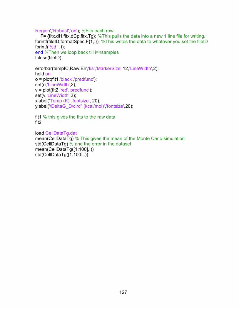
127

Region','Robust','on'); %Fits each row F= {fitx.dH,fitx.dCp,fitx.Tg}; %This pulls the data into a new 1 line file for writing. fprintf(fileID,formatSpec,F{1,:}); %This writes the data to whatever you set the fileID fprintf('%d ', i); end %Then we loop back till i=nsamples fclose(fileID); errorbar(tempIC,Raw,Err,'ks','MarkerSize',12,'LineWidth',2); hold on o = plot(fit1,'black','predfunc'); set(o,'LineWidth',2); v = plot(fit2,'red','predfunc'); set(v,'LineWidth',2); xlabel('Temp (K)','fontsize', 20); ylabel('\DeltaG_D\circ'' (kcal/mol)','fontsize',20); fit1 % this gives the fits to the raw data fit2 load CellDataTg.dat mean(CellDataTg) % This gives the mean of the Monte Carlo simulation std(CellDataTg) % and the error in the dataset mean(CellDataTg([1:100],:)) std(CellDataTg([1:100],:))

128

APPENDIX 3. MONTE CARLO FOR EXTRAPOLATING DATA FROM THE GIBBS-HELMHOLTZ EQUATION TO ANY TEMPERATURE USING KIRCHOFF’S

RELATIONS.

clear all close all temp = 298 nsamples=1e6 %random following gaussian, DILUTE dH=normrnd(19.1,0.3,nsamples,1); dCp=normrnd(0.88,0.02,nsamples,1); T=normrnd(306.7,0.1,nsamples,1); %generate data H=dH+dCp.*(temp-T); TdS= temp.*((dH./T)+dCp.*log(temp./T)); Ts1=exp(log(T)-((dH./T)./dCp)); %mean and STD of data Enthalpy = mean(H) STD = std(H) Entropy = mean(TdS) STD = std(TdS) Ts = mean(Ts1) STD = std(Ts1)

129

APPENDIX 4. T2 FITTING SCRIPT. clear all close all %Script to Measure 19F T2 Rates %Uses a Monte Carlo for error if you take one plane 3 times % AES, 2015 %-----ENTER INFORMATION----- d20 = 0.00025; %Insert echo time p1 = 0.00001275; %Insert pulse length cycles = [2;8;128;4;64;32;16;12]; % # of cycles %Folded State A=[89934,91251,90215]; %Insert 3 repeated delays B=mean(A); Folded = [102385;B;16083;96622;38777;61369;80235;85086]; sigmaF=std(A); covarF=sigmaF^2; %MC uses covariance, which is standard deviation squared CovarF = [covarF covarF covarF covarF covarF covarF covarF covarF]; % Make sure this is the same size as cycles %Unfolded State C=[89841,89795,89109]; D=mean(C); Unfolded = [94371;D;42550;94781;64204;78122;84680;89287]; sigmaU=std(C); covarU=sigmaU^2; CovarU = [covarU covarU covarU covarU covarU covarU covarU covarU]; %MC stuff, can name files whatever, but need to change below if you do nsamples = 10; fileIDF = fopen('Folded.dat','w'); fileIDU = fopen('Unfolded.dat','w'); formatSpec = '%d %d\n'; %Finds Field and Relaxation times tCP = (d20*2) + (p1*2); vCPMG = 1 / (2 * tCP) time = tCP * cycles %-----STARTS DATA ANALYSIS----- T2fit = fittype('(A*exp(-x/T))','independent',{'x'},'coefficients',{'A','T'}); % Declaring the fit: a is overall height, b is T1 T2cfit = fittype('(A*exp(-x/T)+C)','independent',{'x'},'coefficients',{'A','T','C'}); %

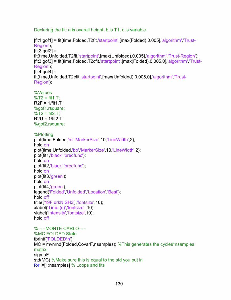
130

Declaring the fit: a is overall height, b is T1, c is variable [fit1,gof1] = fit(time,Folded,T2fit,'startpoint',[max(Folded),0.005],'algorithm','Trust-Region'); [fit2,gof2] = fit(time,Unfolded,T2fit,'startpoint',[max(Unfolded),0.005],'algorithm','Trust-Region'); [fit3,gof3] = fit(time,Folded,T2cfit,'startpoint',[max(Folded),0.005,0],'algorithm','Trust-Region'); [fit4,gof4] = fit(time,Unfolded,T2cfit,'startpoint',[max(Unfolded),0.005,0],'algorithm','Trust-Region'); %Values %T2 = fit1.T; R2F = 1/fit1.T %gof1.rsquare; %T2 = fit2.T; R2U = 1/fit2.T %gof2.rsquare; %Plotting plot(time,Folded,'rs','MarkerSize',10,'LineWidth',2); hold on plot(time,Unfolded,'bo','MarkerSize',10,'LineWidth',2); plot(fit1,'black','predfunc'); hold on plot(fit2,'black','predfunc'); hold on plot(fit3,'green'); hold on plot(fit4,'green'); legend('Folded','Unfolded','Location','Best'); hold off title(['19F drkN SH3'],'fontsize',10); xlabel('Time (s)','fontsize', 10); ylabel('Intensity','fontsize',10); hold off %-----MONTE CARLO----- %MC FOLDED State fprintf('FOLDED\n'); MC = mvnrnd(Folded,CovarF,nsamples); %This generates the cycles*nsamples matrix sigmaF std(MC) %Make sure this is equal to the std you put in for i=[1:nsamples] % Loops and fits

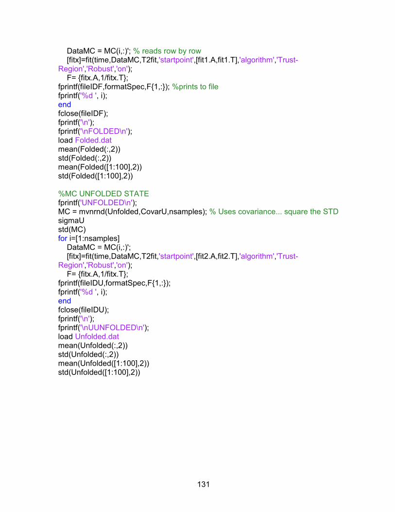
131

DataMC = MC(i,:)'; % reads row by row [fitx]=fit(time,DataMC,T2fit,'startpoint',[fit1.A,fit1.T],'algorithm','Trust-Region','Robust','on'); F= {fitx.A,1/fitx.T}; fprintf(fileIDF,formatSpec,F{1,:}); %prints to file fprintf('%d ', i); end fclose(fileIDF); fprintf('\n'); fprintf('\nFOLDED\n'); load Folded.dat mean(Folded(:,2)) std(Folded(:,2)) mean(Folded([1:100],2)) std(Folded([1:100],2)) %MC UNFOLDED STATE fprintf('UNFOLDED\n'); MC = mvnrnd(Unfolded,CovarU,nsamples); % Uses covariance... square the STD sigmaU std(MC) for i=[1:nsamples] DataMC = MC(i,:)'; [fitx]=fit(time,DataMC,T2fit,'startpoint',[fit2.A,fit2.T],'algorithm','Trust-Region','Robust','on'); F= {fitx.A,1/fitx.T}; fprintf(fileIDU,formatSpec,F{1,:}); fprintf('%d ', i); end fclose(fileIDU); fprintf('\n'); fprintf('\nUUNFOLDED\n'); load Unfolded.dat mean(Unfolded(:,2)) std(Unfolded(:,2)) mean(Unfolded([1:100],2)) std(Unfolded([1:100],2))

132

APPENDIX 5. T1 FITTING SCRIPT. clear all close all time = [0 0.8 0.05 0.1 1.5 0.5 0.25]; %Input mixing time T1 %Folded State A=[22416,19935,22194]; %Insert 3 repeated delays B=mean(A); Folded = [-43866;B;-35112;-27787;37217;3135;-15520]; sigmaF=std(A); covarF=sigmaF^2; %MC uses covariance, which is standard deviation squared CovarF = [covarF covarF covarF covarF covarF covarF covarF]; % Make sure this is the same size as cycles %Unfolded State C=[33151,38388,34403]; D=mean(C); Unfolded = [-83758;D;-75811;-60023;71491;4188;-33815]; sigmaU=std(C); covarU=sigmaU^2; CovarU = [covarU covarU covarU covarU covarU covarU covarU]; %MC stuff, can name files whatever, but need to change below if you do nsamples = 1000; fileIDF = fopen('Folded.dat','w'); fileIDU = fopen('Unfolded.dat','w'); formatSpec = '%d %d %d\n'; %-----STARTS DATA ANALYSIS----- T1fit =fittype('M*(1-V*exp(-x/T))','independent',{'x'},'coefficients',{'M','T','V'}); % Declaring the fit: M is Sz, T is T1, V is fudge factor [fit1,gof1] = fit(time,Folded,T1fit,'startpoint',[max(Folded),0.05,1],'algorithm','Trust-Region'); [fit2,gof2] = fit(time,Unfolded,T1fit,'startpoint',[max(Unfolded),0.05,1],'algorithm','Trust-Region'); %Values

133

%T1 = fit1.T R1F = 1/fit1.T %gof1.rsquare; %T1 = fit2.T R1U = 1/fit2.T %gof2.rsquare; plot(time,Folded,'rs','MarkerSize',10,'LineWidth',2); hold on plot(time,Unfolded,'bo','MarkerSize',10,'LineWidth',2); plot(fit1,'black'); hold on plot(fit2,'black'); legend('Folded','Unfolded','Location','Best'); hold off title(['19F drkN SH3'],'fontsize',10); xlabel('Time (s)','fontsize', 10); ylabel('Volume','fontsize',10); %axis([0 1.6 -50000 50000]); % x- axis, y-axis hold off %-----MONTE CARLO----- %MC FOLDED State fprintf('FOLDED\n'); MC = mvnrnd(Folded,CovarF,nsamples); % Uses covariance... square the STD std(MC); for i=[1:nsamples] DataMC = MC(i,:)'; [fitx]=fit(time,DataMC,T1fit,'startpoint',[fit1.M,fit1.T,fit1.V],'algorithm','Trust-Region','Robust','on'); F= {fitx.M,1/fitx.T,fitx.V}; fprintf(fileIDF,formatSpec,F{1,:}); fprintf('%d ', i); end fclose(fileIDF); fprintf('\n'); fprintf('\nFOLDED\n'); load Folded.dat mean(Folded(:,2)) std(Folded(:,2)) mean(Folded([1:100],2)) std(Folded([1:100],2)) %MC UNFOLDED STATE fprintf('UNFOLDED\n'); MC = mvnrnd(Unfolded,CovarU,nsamples); % Uses covariance... square the STD

134

std(MC); for i=[1:nsamples] DataMC = MC(i,:)'; [fitx]=fit(time,DataMC,T1fit,'startpoint',[fit2.M,fit2.T,fit2.V],'algorithm','Trust-Region','Robust','on'); F= {fitx.M,1/fitx.T,fitx.V}; fprintf(fileIDU,formatSpec,F{1,:}); fprintf('%d ', i); end fclose(fileIDU); fprintf('\n'); fprintf('\nUUNFOLDED\n'); load Unfolded.dat mean(Unfolded(:,2)) std(Unfolded(:,2)) mean(Unfolded([1:100],2)) std(Unfolded([1:100],2))

135

APPENDIX 6.1. SCRIPT FOR FITTING T1 AND T2 DATA USING A MODEL FREE APPROACH TO OBTAIN TUMBLING TIMES.

Calls on Appendix 6.2 and 6.3, ensure they are in the same folder as 6.1. clear all; close all; global R1F R2F R1U R2U % experimental R1 global calc_R1F calc_R2F calc_R1U calc_R2U % obtained by simulations of R1 global err2 err3 % error global r tm te S global MCR1F MCR1U MCR2F MCR2U nsamples = 1000; fileIDF = fopen('Foldedtm.dat','w'); fileIDU = fopen('Unfoldedtm.dat','w'); formatSpec = '%d %d %d\n'; % R1F=normrnd(1.46,0.08,nsamples,1); % R1 Folded R2F=normrnd(165,27,nsamples,1); % R2 Folded R1U=normrnd(1.37,0.05,nsamples,1); % R1 unfolded R2U=normrnd(110,8,nsamples,1); % R2 unfolded % ---------------- END OF INPUT ----------------- % --- FIT --- fprintf('\nFOLDED:\n') for i=[1:nsamples] MCR1F = R1F(i,:); MCR2F = R2F(i,:); r = 2.0; tm = 5e-9; te = 50e-12; S = 0.9; x0 = [r,tm]; minopt = optimset('TolX',1e-14,'TolFun',1e-14,'MaxFunEvals',1e10,'MaxIter',1e10); x=fminsearch('F19_Folded_tc_equation_MC',x0,minopt); Ans= {x(1),x(2),err2}; fprintf(fileIDF,formatSpec,Ans{1,:}); % prints to file %fprintf('%d ', i); end

136

load Foldedtm.dat; fprintf('\nF-H distance (A) = '); mean(Foldedtm(:,1)) std(Foldedtm(:,1)) fprintf('\nCorrelation time (ns) = '); mean(Foldedtm(:,2)) std(Foldedtm(:,2)) fprintf('\nInternal motion (ps) = '); fprintf('%d\n',20); fprintf('Order parameter = '); fprintf('%d\n',0.82); fprintf('Error = '); fprintf('%d\n', err2); fprintf('\n') fprintf('\nUNFOLDED:\n') for i=[1:nsamples] MCR1U = R1U(i,:); MCR2U = R2U(i,:); r = 2.0; tm = 5e-9; te = 50e-12; S = 0.9; x0 = [r,tm]; minopt = optimset('TolX',1e-14,'TolFun',1e-14,'MaxFunEvals',1e10,'MaxIter',1e10); x=fminsearch('F19_Unfolded_tc_equation_MC',x0,minopt); Ans= {x(1),x(2),err3}; fprintf(fileIDU,formatSpec,Ans{1,:}); % prints to file %fprintf('%d ', i); end load Unfoldedtm.dat; fprintf('\nF-H distance (A) = '); mean(Unfoldedtm(:,1)) std(Unfoldedtm(:,1)) fprintf('\nCorrelation time (ns) = '); mean(Unfoldedtm(:,2)) std(Unfoldedtm(:,2))

137

fprintf('\nInternal motion (ps) = '); fprintf('%d\n',1200); fprintf('Order parameter = '); fprintf('%d\n',0.32); fprintf('Error = '); fprintf('%d\n', err3); fprintf('\n')

138

APPENDIX 6.2. SPECTRAL DENSITY FUNCTIONS FOR THE FOLDED STATE. % Equations were modified from Li, Chemistry. 2013,19(38):12705-10. doi: 10.1002/chem.201301657. % CSA (-93.5) and n (0.24) were taken from London, JBNMR 1996, 7, 261 % CSA (42.2) and n (0.27) were taken from Durr, JMR 2008, 191, 7-15 % te and S were taken from Farrow, Biochemistry 1995, 34, 868 function chi2=chi2_simple(xarg); global MCR1F MCR2F global calc_R1F calc_R2F global err2 global r tm te S r = xarg(1); %in Angstrom tm = xarg(2); te = 20e-12; S = 0.82; wF= 470530000 * 2*pi; %rad/s wH= 500120000 * 2*pi; %rad/s dO= -93.5; % CSA ppm n= 0.24; % asymmetry, 0.2-0.4 gH= 42576000; % /s/T gF= 40052000; % /s/T yF= 251790000; %rad/s/T yH= 267530000; %rad/s/T uo= 4*pi*10^-7; % T2 * m3 * J-1 hbar = 1.054571726 * 10^-34; % J * s C = (((uo/(4*pi))*hbar*yF*yH)/(r*10^-10)^3); % F-H dipolar coupling constant CSA = wF^2*(dO/1000000)^2*(1+((n^2)/3)); % CSA t=1/((1/tm)+(1/te)); %Spectral density functions JwF = (((S*tm)/(1+((wF*tm)^2)))+((((1-S)*t)/(1+((wF*t)^2))))); JwH = (((S*tm)/(1+((wH*tm)^2)))+((((1-S)*t)/(1+((wH*t)^2))))); JwFmwH = (((S*tm)/(1+(((wF-wH)*tm)^2)))+((((1-S)*t)/(1+(((wF-wH)*t)^2))))); JwFpwH = (((S*tm)/(1+(((wF+wH)*tm)^2)))+((((1-S)*t)/(1+(((wF+wH)*t)^2))))); J0 = ((S*tm)+((1-S)*t));

139

%Calculate relaxation rates calc_R1F = ((C^2/10)*[(3*JwF)+JwFmwH+(6*JwFpwH)])+((2/15)*JwF*CSA); calc_R2F = ((C^2/20)*[(4*J0)+(3*JwF)+JwFmwH+(6*JwH)+(6*JwFpwH)])+((1/45)*CSA*[(3*JwF)+(4*J0)]); %This had a CSA multiplier of 2/15 %Error ChiR1=(calc_R1F-MCR1F).^2; ChiR2=(calc_R2F-MCR2F).^2; chi2=ChiR1+ChiR2; err2=sqrt(chi2);

140

APPENDIX 6.3. SPECTRAL DENSITY FUNCTIONS FOR THE UNFOLDED STATE.

% Equations were modified from Li, Chemistry. 2013,19(38):12705-10. doi: 10.1002/chem.201301657. % CSA (-93.5) and n (0.24) were taken from London, JBNMR 1996, 7, 261 % CSA (42.2) and n (0.27) were taken from Durr, JMR 2008, 191, 7-15 % te and S were taken from Farrow, Biochemistry 1995, 34, 868 function chi2=chi2_simple(xarg); global MCR1U MCR2U global calc_R1U calc_R2U global err3 global r tm te S r = xarg(1); %in Angstrom tm = xarg(2); te = 1200-12; S = 0.32; wF= 470530000 * 2*pi; %rad/s wH= 500120000 * 2*pi; %rad/s dO= -93.5; % CSA ppm n= 0.24; % asymmetry, 0.2-0.4 gH= 42576000; % /s/T gF= 40052000; % /s/T yF= 251790000; %rad/s/T yH= 267530000; %rad/s/T uo= 4*pi*10^-7; % T2 * m3 * J-1 hbar = 1.054571726 * 10^-34; % J * s C = (((uo/(4*pi))*hbar*yF*yH)/(r*10^-10)^3); % F-H dipolar coupling constant CSA = wF^2*(dO/1000000)^2*(1+((n^2)/3)); % CSA t=1/((1/tm)+(1/te)); %Spectral density functions JwF = (((S*tm)/(1+((wF*tm)^2)))+((((1-S)*t)/(1+((wF*t)^2))))); JwH = (((S*tm)/(1+((wH*tm)^2)))+((((1-S)*t)/(1+((wH*t)^2))))); JwFmwH = (((S*tm)/(1+(((wF-wH)*tm)^2)))+((((1-S)*t)/(1+(((wF-wH)*t)^2))))); JwFpwH = (((S*tm)/(1+(((wF+wH)*tm)^2)))+((((1-S)*t)/(1+(((wF+wH)*t)^2))))); J0 = ((S*tm)+((1-S)*t));

141

%Calculate relaxation rates calc_R1U = ((C^2/10)*[(3*JwF)+JwFmwH+(6*JwFpwH)])+((2/15)*JwF*CSA); calc_R2U = ((C^2/20)*[(4*J0)+(3*JwF)+JwFmwH+(6*JwH)+(6*JwFpwH)])+((1/45)*CSA*[(3*JwF)+(4*J0)]); %This had a CSA multiplier of 2/15 %Error ChiR1=(calc_R1U-MCR1U).^2; ChiR2=(calc_R2U-MCR2U).^2; chi2=ChiR1+ChiR2; err3=sqrt(chi2);

142

APPENDIX 7.1. SCRIPT FOR FITTING EXCHANGE SPECTROSCOPY DATA. Calls on Appendix 7.2 and 7.3, ensure they are in the same folder as 7.1. % Fit for Slow exchange % drkN SH3, F19 % by AES % Can set R1 to value attained from inversion recovery sequence if desired. clear all close all global tmix % exchange time, in seconds global expt_FF_pk expt_UU_pk % experimental self peaks global expt_FU_pk expt_UF_pk % experimental cross peaks global calc_FF_pk calc_UU_pk % obtained by simulations of self peaks global calc_FU_pk calc_UF_pk % obtained by simulations of cross peaks global tmix_plot % array of exchange times used for plotting global err2 % error global calc_FF_pk_plot calc_UU_pk_plot calc_FU_pk_plot calc_UF_pk_plot % plots fits global DataFF DataUU % MC self peaks global DataFU DataUF % MC cross peaks tmix=[0.300 0.140 0.800 0.0015 0.210 0.070 0.500]; % exchange times, in seconds FF=[146271,144431,103987]; % insert triplicate delays UU=[915785,928604,847891]; FU=[53659,51912,51386]; UF=[15430,14034,13400]; A=mean(FF); % calculates the average of the triplicates B=mean(UU); C=mean(FU); D=mean(UF); expt_FF_pk=[72815 A 15682 271150 109976 195355 34026]; % extracting experimental FF points expt_UU_pk=[698989 B 320137 1220349 831850 1052992 519585]; % extracting experimental UU points expt_FU_pk=[68907 C 44151 3555 60381 28220 60108]; % extracting cross peaks expt_UF_pk=[93498 D 50937 19080 71081 58115 69447]; % extracting cross peaks sigmaFF=std(FF); % calculates the standard deviation of the triplicates

143

sigmaUU=std(UU); sigmaFU=std(FU); sigmaUF=std(UF); covarFF=sigmaFF^2; %MC uses covariance, which is standard deviation squared covarUU=sigmaUU^2; covarFU=sigmaFU^2; covarUF=sigmaUF^2; CovarFF = [covarFF covarFF covarFF covarFF covarFF covarFF covarFF]; % Make sure this is the same size as tmix CovarUU = [covarUU covarUU covarUU covarUU covarUU covarUU covarUU]; CovarFU = [covarFU covarFU covarFU covarFU covarFU covarFU covarFU]; CovarUF = [covarUF covarUF covarUF covarUF covarUF covarUF covarUF]; %MC stuff, can name files whatever, but need to change below if you do nsamples = 100; fileIDF = fopen('Exchange.dat','w'); formatSpec = '%d %d %d %d %d %d %d %d %d\n'; % This will depend on if you allow R1 to vary or if you set it %formatSpec = '%d %d %d %d %d %d %d\n'; % This will depend on if you allow R1 to vary or if you set it % ---------------- END OF INPUT ----------------- % --- FIT --- MCFF = mvnrnd(expt_FF_pk,CovarFF,nsamples); % This generates the MC matrix sigmaFF % Actual sample standard deviation std(MCFF) % MC standard deviation, make sure it matches the actual standard deviation MCUU = mvnrnd(expt_UU_pk,CovarUU,nsamples); MCFU = mvnrnd(expt_FU_pk,CovarFU,nsamples); MCUF = mvnrnd(expt_UF_pk,CovarUF,nsamples); for i=[1:nsamples] % Loops and fits DataFF = MCFF(i,:); % reads row by row DataUU = MCUU(i,:); DataFU = MCFU(i,:); DataUF = MCUF(i,:); Izf = max(DataFF); % Folded decay curve initial amplitude Izu = max(DataUU); % Unfolded decay curve initial amplitude kfu = 3; % unfolding rate kuf = 0.5; % folding rate R1f = 1.8; % R1 guess for folded R1u = 1.5; % R1 guess for unfolded

144

Efu = min(DataFU); % Leakage, if the 0ms point gives a buildup peak Euf = min(DataUF); % Leakage, if the 0ms point gives a buildup peak x0 = [kfu, kuf, Izf, Izu, Efu, Euf, R1f,R1u]; % declaring variables to minimize %x0 = [kfu, kuf, Izf, Izu, Efu, Euf]; % declaring variables to minimize with R1 set minopt = optimset('TolX',1e-6,'TolFun',1e-6,'MaxFunEvals',1e6,'MaxIter',1e6); x=fminsearch('chi2_simple35_F19_MC',x0,minopt); Ans= {x(1),x(2),x(3),x(4),x(5),x(6),x(7),x(8),err2}; % vary R1 %Ans= {x(1),x(2),x(3),x(4),x(5),x(6),err2}; % dont vary R1 fprintf(fileIDF,formatSpec,Ans{1,:}); %prints to file fprintf('%d ', i); end load Exchange.dat; fprintf('\nkunfold\n'); mean(Exchange(:,1)) std(Exchange(:,1)) fprintf('\nkfold\n'); mean(Exchange(:,2)) std(Exchange(:,2)) fprintf('\nR1F\n'); % comment and uncomment depending on if you vary R1 mean(Exchange(:,7)) std(Exchange(:,7)) fprintf('\nR1U\n'); % comment and uncomment depending on if you vary R1 mean(Exchange(:,8)) std(Exchange(:,8)) % Plotting figure(1); plot(tmix,expt_FF_pk,'rs', 'MarkerSize',14,'Linewidth',4); hold on plot(tmix,expt_UU_pk,'bo','MarkerSize',14,'Linewidth',4); hold on plot(tmix,expt_FU_pk,'rs', 'MarkerSize',14,'Linewidth',4); hold on plot(tmix,expt_UF_pk,'bo','MarkerSize',14,'Linewidth',4); tmix_plot=linspace(min(tmix),max(tmix),200); Izf = mean(Exchange(:,3)); % Decay curve initial amplitude Izu = mean(Exchange(:,4)); % Buildup curve initial amplitude kfu = mean(Exchange(:,1)); % kfu

145

kuf = mean(Exchange(:,2)); % kuf %R1f = 1.8; % R1 guess for folded %R1u = 1.5; % R1 guess for unfolded R1f = mean(Exchange(:,7)); % R1 guess for folded R1u = mean(Exchange(:,8)); % R1 guess for unfolded Efu = mean(Exchange(:,5)); % Leakage, if the 0ms point gives a buildup peak Euf = mean(Exchange(:,6)); % Leakage, if the 0ms point gives a buildup peak chi2_simple_plot35_F19(x); plot(tmix_plot,calc_FF_pk_plot,'k-','Linewidth', 2); plot(tmix_plot,calc_UU_pk_plot,'k-','Linewidth',2); plot(tmix_plot,calc_FU_pk_plot,'k-','Linewidth', 2); plot(tmix_plot,calc_UF_pk_plot,'k-','Linewidth',2); fig_leg=legend('FF','UU','FU','UF','Location','Best'); set(fig_leg,'FontSize',18,'fontweight','bold','Box','off'); hold off tit=[' 19F drkN SH3 ', ' error = ', num2str(err2)]; title(tit,'fontsize',20); xlabel('Time (s)','fontsize', 20); ylabel('Intensity','fontsize',20); set(gca,'fontsize',18); %fn0 = ['Dilute_EXSY_022315.eps']; %print( gcf, '-depsc2', fn0 ) hold off

146

APPENDIX 7.2. EVOLUTION EQUATIONS FOR EXCHANGE SPECTROSCOPY. % Equations were taken from Farrow, J. Bio. NMR, 4 (1994) 727-734 function chi2=chi2_simple(xarg); global tmix global DataFF DataUU % MC self peaks global DataFU DataUF % MC cross peaks global calc_FF_pk calc_UU_pk calc_FU_pk calc_UF_pk global err2 kfu=xarg(1); kuf=xarg(2); Izf=xarg(3); Izu=xarg(4); Efu=xarg(5); Euf=xarg(6); %R1f=1.8; % Set to value if desired, ie R1f=[2.4]; %R1u=1.5; % Set to value if desired. R1f=xarg(7); % Set to value if desired, ie R1f=[2.4]; R1u=xarg(8); a11 = R1f + kfu; a22 = R1u + kuf; a12 = -kuf; a21 = -kfu; L1 = [(1/2)*((a11+a22)+((a11-a22)^2+4*kfu*kuf).^(1/2))]; L2 = [(1/2)*((a11+a22)-((a11-a22)^2+4*kfu*kuf).^(1/2))]; for i=1:length(tmix) FF=(Izf*(-(L2-a11)*exp(-L1*tmix(i))+(L1-a11)*exp(-L2*tmix(i)))/(L1-L2)); UU=(Izu*(-(L2-a22)*exp(-L1*tmix(i))+(L1-a22)*exp(-L2*tmix(i)))/(L1-L2)); FU=(Efu+Izf*((a21*exp(-L1*tmix(i)))-(a21*exp(-L2*tmix(i))))/(L1-L2)); UF=(Euf+Izu*((a12*exp(-L1*tmix(i)))-(a12*exp(-L2*tmix(i))))/(L1-L2)); calc_FF_pk(i)=FF(1); calc_UU_pk(i)=UU(1); calc_FU_pk(i)=FU(1); calc_UF_pk(i)=UF(1); end;

147

ChiFF=sum((calc_FF_pk-DataFF).^2); ChiUU=sum((calc_UU_pk-DataUU).^2); ChiFU=sum((calc_FU_pk-DataFU).^2); ChiUF=sum((calc_UF_pk-DataUF).^2); chi2=ChiFF+ChiUU+ChiFU+ChiUF; err2=sqrt(chi2);

148

APPENDIX 7.3. EXCHANGE SPECTROSCOPY PLOTTING SCRIPT. function dummy=chi2_simple_plot(xarg); global tmix_plot global calc_FF_pk_plot calc_UU_pk_plot calc_FU_pk_plot calc_UF_pk_plot kfu=xarg(1); kuf=xarg(2); Izf=xarg(3); Izu=xarg(4); Efu=xarg(5); Euf=xarg(6); %R1f=1.8; % Set to value if desired, ie R1f=[2.4]; %R1u=1.5; % Set to value if desired. R1f=xarg(7); % Set to value if desired, ie R1f=[2.4]; R1u=xarg(8); a11 = R1f + kfu; a22 = R1u + kuf; a12 = -kuf; a21 = -kfu; L1 = [(1/2)*((a11+a22)+((a11-a22)^2+4*kfu*kuf).^(1/2))]; L2 = [(1/2)*((a11+a22)-((a11-a22)^2+4*kfu*kuf).^(1/2))]; for i=1:length(tmix_plot) FF=(Izf*(-(L2-a11)*exp(-L1*tmix_plot(i))+(L1-a11)*exp(-L2*tmix_plot(i)))/(L1-L2)); UU=(Izu*(-(L2-a22)*exp(-L1*tmix_plot(i))+(L1-a22)*exp(-L2*tmix_plot(i)))/(L1-L2)); FU=(Efu+Izf*((a21*exp(-L1*tmix_plot(i)))-(a21*exp(-L2*tmix_plot(i))))/(L1-L2)); UF=(Euf+Izu*((a12*exp(-L1*tmix_plot(i)))-(a12*exp(-L2*tmix_plot(i))))/(L1-L2)); calc_FF_pk_plot(i)=FF(1); calc_UU_pk_plot(i)=UU(1); calc_FU_pk_plot(i)=FU(1); calc_UF_pk_plot(i)=UF(1); end;

149

REFERENCES

1 Zimmerman, S. B. & Trach, S. O. Estimation of macromolecule concentrations and excluded volume effects for the cytoplasm of Escherichia coli. Journal of Molecular Biology 222, 599-620 (1991).

2 Theillet, F.-X., Binolfi, A., Frembgen-Kesner, T., Hingorani, K., Sarkar, M., Kyne, C., Li, C., Crowley, P., Gierasch, L. M., Pielak, G. J., Elcock, A. H., Gershenson, A. & Selenko, P. Physicochemical properties of cells and thier effects on intrinsically disordered proteins (IDPs). Chemical Reviews 114, 6661-6714 (2014).

3 Srere, P. A. The infrastructure of the mitochondrial matrix. Trends in Biochemical Sciences 5, 120-121 (1980).

4 Spitzer, J. & Poolman, B. The role of biomacromolecular crowding, ionic strength, and physicochemical gradients in the complexities of life's emergence. Microbiology and Molecular Biology Reviews 73, 371-388 (2009).

5 Waudby, C. A., Camilloni, C., Fitzpatrick, A. W. P., Cabrita, L. D., Dobson, C. M., Vendruscolo, M. & Christodoulou, J. In-cell NMR characterization of the secondary structure populations of a disordered conformation of α-synuclein within E. coli cells. PLoS ONE 8, e72286 (2013).

6 London, R. E., Gregg, C. T. & Matwiyoff, N. A. Nuclear magnetic resonance of rotational mobility of mouse hemoglobin labeled with [2-13C] histidine. Science 188, 266-268 (1975).

7 Llinas, M., Wüthrich, K., Schwotzer, W. & Von Philipsborn, W. 15N nuclear magnetic resonance of living cells. Nature 257, 817-818 (1975).

8 Brindle, K. M., Williams, S.-P. & Boulton, M. 19F NMR detection of a fluorine-labelled enzyme in vivo. FEBS Letters 255, 121-124 (1989).

9 Daniels, A., Williams, R. J. & Wright, P. E. Nuclear magnetic resonance studies of the adrenal gland and some other organs. Nature 261, 321-323 (1976).

150

10 Brown, F. F., Campbell, I. D., Kuchel, P. W. & Rabenstein, D. C. Human erythrocyte metabolism studies by 1H spin echo NMR. FEBS Letters 82, 12-16 (1977).

11 Serber, Z. & Dötsch, V. In-cell NMR spectroscopy. Biochemistry 40, 14317-14323 (2001).

12 Serber, Z., Ledwidge, R., Miller, S. M. & Dötsch, V. Evaluation of Parameters Critical to Observing Proteins Inside Living Escherichia coli by In-Cell NMR Spectroscopy. Journal of the American Chemical Society 123, 8895-8901 (2001).

13 Freedberg, D. & Selenko, P. Live cell NMR. Annual Review of Biophysics 43, 171-192 (2014).

14 Hänsel, R., Luh, L. M., Corbeski, I., Trantirek, L. & Dötsch, V. In-cell NMR and EPR spectroscopy of biomacromolecules. Angewandte Chemie International Edition (2014).

15 Tochio, H. Watching protein structure at work in living cells using NMR spectroscopy. Current Opinion in Chemical Biology 16, 609-613 (2012).

16 Pielak, G. J. & Tian, F. Membrane proteins, magic-angle spinning, and in-cell NMR. Proceedings of the National Academy of Sciences USA 109, 4715-4716 (2012).

17 Ma, J., McLeod, S., MacCormack, K., Sriram, S., Gao, N., Breeze, A. L. & Hu, J. Real-time monitoring of New Delhi metallo-β-Lactamase activity in living cacterial cells by 1H NMR spectroscopy. Angewandte Chemie International Edition 53, 2130-2133 (2014).

18 Anfinsen, C. B. Principles that govern the folding of protein chains. Science 181, 223-230 (1973).

19 McConkey, E. Molecular evolution, intracellular organization, and the quinary structure of proteins. Proceedings of the National Academy of Sciences USA 79, 3236-3240 (1982).

151

20 Srere, P. A. The metabolon. Trends in Biochemical Sciences 10, 109-110 (1985).

21 Wirth, A. J. & Gruebele, M. Quinary protein structure and the consequences of crowding in living cells: Leaving the test-tube behind. BioEssays 35, 984-993 (2013).

22 Gershenson, A. Deciphering protein stability in cells. Journal of Molecular Biology 426, 4-6 (2014).

23 Li, C., Charlton, L. M., Lakkavaram, A., Seagle, C., Wang, G., Young, G. B., Macdonald, J. M. & Pielak, G. J. Differential dynamical effects of macromolecular crowding on an intrinsically disordered protein and a globular protein: Implications for in-cell NMR spectroscopy. Journal of the American Chemical Society 130, 6310-6311 (2008).

24 Barnes, C. O. & Pielak, G. J. In-cell protein NMR and protein leakage. Proteins: Structure, Function, and Bioinformatics 79, 347-351 (2011).

25 Waudby, C. A., Mantle, M. D., Cabrita, L. D., Gladden, L. F., Dobson, C. M. & Christodoulou, J. Rapid distinction of intracellular and extracellular proteins using NMR diffusion measurements. Journal of the American Chemical Society 134, 11312-11315 (2012).

26 Reardon, P. N. & Spicer, L. D. Multidimensional NMR spectroscopy for protein characterization and assignment inside cells. Journal of the American Chemical Society 127, 10848-10849 (2005).

27 Sakakibara, D., Sasaki, A., Ikeya, T., Hamatsu, J., Hanashima, T., Mishima, M., Yoshimasu, M., Hayashi, N., Mikawa, T. & Wälchli, M. Protein structure determination in living cells by in-cell NMR spectroscopy. Nature 458, 102-105 (2009).

28 Crowley, P. B., Chow, E. & Papkovskaia, T. Protein interactions in the Escherichia coli cytosol: an impediment to in-cell NMR spectroscopy. ChemBioChem 12, 1043-1048 (2011).

29 Crowley, P. B., Kyne, C. & Monteith, W. B. Simple and inexpensive incorporation of 19F-Tryptophan for protein NMR spectroscopy. Chemical Communications 48, 10681-10683 (2012).

152

30 Hamatsu, J., O’Donovan, D., Tanaka, T., Shirai, T., Hourai, Y., Mikawa, T., Ikeya, T., Mishima, M., Boucher, W., Smith, B. O., Laue, E. D., Shirakawa, M. & Ito, Y. High-resolution heteronuclear multidimensional NMR of proteins in living insect cells using a baculovirus protein expression system. Journal of the American Chemical Society 135, 1688-1691 (2013).

31 Li, C., Wang, G.-F., Wang, Y., Creager-Allen, R., Lutz, E. A., Scronce, H., Slade, K. M., Ruf, R. A. S., Mehl, R. A. & Pielak, G. J. Protein 19F NMR in Escherichia coli. Journal of the American Chemical Society 132, 321-327 (2010).

32 Wang, Q., Zhuravleva, A. & Gierasch, L. M. Exploring weak, transient protein-protein interactions in crowded in vivo environments by in-cell nuclear magnetic resonance spectroscopy. Biochemistry 50, 9225-9236 (2011).

33 Xu, G., Ye, Y., Liu, X., Cao, S., Wu, Q., Cheng, K., Liu, M., Pielak, G. J. & Li, C. Strategies for Protein NMR in Escherichia coli. Biochemistry 53, 1971-1981 (2014).

34 Kosol, S., Contreras-Martos, S., Cedeño, C. & Tompa, P. Structural characterization of intrinsically disordered proteins by NMR spectroscopy. Molecules 18, 10802-10828 (2013).

35 Luh, L. M., Haensel, R., Loehr, F., Kirchner, D. K., Krauskopf, K., Pitzius, S., Schaefer, B., Tufar, P., Corbeski, I., Guentert, P. & Dötsch, V. Molecular crowding drives active Pin1 into nonspecific complexes with endogenous proteins prior to substrate recognition. Journal of the American Chemical Society 135, 13796-13803 (2013).

36 Latham, M. P. & Kay, L. E. Is buffer a good proxy for a crowded cell-like environment? A comparative NMR study of calmodulin side-chain dynamics in buffer and E. coli Lysate. PLoS ONE 7, e48226 (2012).

37 Latham, M. P. & Kay, L. E. Probing non-specific interactions of Ca2+-calmodulin in E. coli lysate. Journal of Biomolecular NMR 55, 239-247 (2013).

38 Reckel, S., Lopez, J. J., Löhr, F., Glaubitz, C. & Dötsch, V. In-cell solid-state NMR as a tool to study proteins in large complexes. ChemBioChem 13, 534-537 (2012).

153

39 Zhao, X. Protein structure determination by solid-state NMR. Topics in Current Chemistry 326, 187–214 (2012).

40 Latham, M. P. & Kay, L. E. A similar in vitro and in cell-lysate folding intermediate for the FF domain. Journal of Molecular Biology (2014).

41 Sekhar, A., Latham, M. P., Vallurupalli, P. & Kay, L. E. Viscosity-dependent kinetics of protein conformational exchange: microviscosity effects and the need for a small viscogen. Journal of Physical Chemistry B 118, 4546-4551 (2014).

42 Wang, Y., Li, C. & Pielak, G. J. Effects of proteins on protein diffusion. Journal of the American Chemical Society 132, 9392-9397 (2010).

43 Majumder, S., DeMott, C. M., Burz, D. S. & Shekhtman, A. Using singular value decomposition to characterize protein–protein interactions by in-cell NMR spectroscopy. ChemBioChem 15, 929-933 (2014).

44 O'Hagan, D. & Harper, D. B. Fluorine-containing natural products. Journal of Fluorine Chemistry 100, 127-133 (1999).

45 Gerig, J. T. Fluorine NMR of proteins. Progress in Nuclear Magnetic Resonance Spectroscopy 26, Part 4, 293-370 (1994).

46 Khan, F., Kuprov, I., Craggs, T. D., Hore, P. J. & Jackson, S. E. 19F NMR studies of the native and denatured states of green fluorescent protein. Journal of the American Chemical Society 128, 10729-10737 (2006).

47 Schlesinger, A. P., Wang, Y., Tadeo, X., Millet, O. & Pielak, G. J. Macromolecular crowding fails to fold a globular protein in cells. Journal of the American Chemical Society 133, 8082-8085 (2011).

48 Englander, S. W. & Kallenbach, N. R. Hydrogen exchange and structural dynamics of proteins and nucleic acids. Quarterly Reviews of Biophysics 16, 521-655 (1983).

49 Hernandez, G. & LeMaster, D. M. NMR analysis of native-state protein conformational flexibility by hydrogen exchange. Methods in Molecular Biology 490, 285-310 (2009).

154

50 Skinner, J. J., Lim, W. K., Bédard, S., Black, B. E. & Englander, S. W. Protein hydrogen exchange: Testing current models. Protein Science 21, 987-995 (2012).

51 Miklos, A. C., Li, C. & Pielak, G. J. Using NMR-detected backbone amide 1H exchange to assess macromolecular crowding effects on globular-protein stability. Methods in Enzymology 466, 1-18 (2009).

52 Smith, A. E., Sarkar, M., Young, G. B. & Pielak, G. J. Amide proton exchange of a dynamic loop in cell extracts. Protein Science 22, 1313-1319 (2013).

53 Benton, L. A., Smith, A. E., Young, G. B. & Pielak, G. J. Unexpected effects of macromolecular crowding on protein stability. Biochemistry 51, 9773-9775 (2012).

54 Smith, A. E., Zhou, L. Z. & Pielak, G. J. Hydrogen exchange of disordered proteins in Escherichia coli. Protein Science 24, 706-713 (2015).

55 Miklos, A. C., Li, C., Sharaf, N. G. & Pielak, G. J. Volume exclusion and soft interaction effects on protein stability under crowded conditions. Biochemistry 49, 6984-6991 (2010).

56 Sanfelice, D., Politou, A., Martin, S. R., Rios, P. D. L., Temussi, P. & Pastore, A. The effect of crowding and confinement: a comparison of Yfh1 stability in different environments. Physical Biology 10, 045002 (2013).

57 Sarkar, M., Smith, A. E. & Pielak, G. J. Impact of reconstituted cytosol on protein stability. Proceedings of the National Academy of Sciences USA 110, 19342-19347 (2013).

58 Inomata, K., Ohno, A., Tochio, H., Isogai, S., Tenno, T., Nakase, I., Takeuchi, T., Futaki, S., Ito, Y., Hiroaki, H. & Shirakawa, M. High-resolution multi-dimensional NMR spectroscopy of proteins in human cells. Nature 458, 106-109 (2009).

59 Sarkar, M., Lu, J. & Pielak, G. J. Protein crowder charge and protein stability. Biochemistry 53, 1601-1606 (2014).

155

60 Sarkar, M. & Pielak, G. J. An osmolyte mitigates the destabilizing effect of protein crowding. Protein Science 23, 1161-1164 (2014).

61 Monteith, W. B. & Pielak, G. J. Residue level quantification of protein stability in living cells. Proceedings of the National Academy of Sciences USA 111, 11335-11340 (2014).

62 Ghaemmaghami, S. & Oas, T. G. Quantitative protein stability measurement in vivo. Nature Structural Biology 8, 879-882 (2001).

63 Monteith, W. B., Cohen, R. D., Smith, A. E., Guzman-Cisneros, E. & Pielak, G. J. Quinary structure modulates protein stability in cells. Proceedings of the National Academy of Sciences USA 112, 1739-1742 (2015).

64 Bertrand, K., Reverdatto, S., Burz, D. S., Zitomer, R. & Shekhtman, A. Structure of proteins in eukaryotic compartments. Journal of the American Chemical Society 134, 12798-12806 (2012).

65 Kubo, S., Nishida, N., Udagawa, Y., Takarada, O., Ogino, S. & Shimada, I. A gel-encapsulated bioreactor system for NMR studies of protein–protein interactions in living mammalian cells. Angewandte Chemie International Edition 52, 1208-1211 (2013).

66 Banci, L., Barbieri, L., Luchinat, E. & Secci, E. Visualization of redox-controlled protein fold in living cells. Chemistry and Biology 20, 747-752 (2013).

67 Banci, L., Barbieri, L., Bertini, I., Luchinat, E., Secci, E., Zhao, Y. & Aricescu, A. R. Atomic-resolution monitoring of protein maturation in live human cells by NMR. Nature Chemical Biology 9, 297-299 (2013).

68 Barbieri, L., Luchinat, E. & Banci, L. Structural insights of proteins in sub-cellular compartments: in-mitochondria NMR. Biochimica et Biophysica Acta 1843, 2492-2496 (2014).

69 Danielsson, J., Inomata, K., Murayama, S., Tochio, H., Lang, L., Shirakawa, M. & Oliveberg, M. Pruning the ALS-associated protein SOD1 for in-cell NMR. Journal of the American Chemical Society 135, 10266-10269 (2013).

156

70 Bekei, B. In-cell NMR spectroscopy in mammalian cells Doctor rerum naturalium thesis, Freie Universität Berlin, (2013).

71 Kiehn, E. D. & Holland, J. J. Size distribution of polypeptide chains in cells. Nature 226, 544-545 (1970).

72 Minton, A. P. Models for excluded volume interaction between an unfolded protein and rigid macromolecular cosolutes: Macromolecular crowding and protein stability revisited. Biophysical Journal 88, 971-985 (2005).

73 McGuffee, S. R. & Elcock, A. H. Diffusion, crowding & protein stability in a dynamic molecular model of the bacterial cytoplasm. PLoS Computational Biology 6, e1000694 (2010).

74 Zhou, H. X., Rivas, G. & Minton, A. P. Macromolecular crowding and confinement: biochemical, biophysical, and potential physiological consequences. Annual Review of Biophysics 37, 375-397 (2008).

75 Elcock, A. H. Models of macromolecular crowding effects and the need for quantitative comparisons with experiment. Current Opinion in Structural Biology 20, 196-206 (2010).

76 Hvidt, A. & Linderstrøm-Lang, K. Exchange of hydrogen atoms in insulin with deuterium atoms in aqueous solutions. Biochimica et Biophysica Acta 14, 574-575 (1954).

77 Berger, A. & Linderstrøm-Lang, K. Deuterium exchange of poly-DL-alanine in aqueous solution. Archives of Biochemistry and Biophysics 69, 106-118 (1957).

78 Englander, S. W., Mayne, L., Bai, Y. & Sosnick, T. R. Hydrogen exchange: the modern legacy of Linderstrøm-Lang. Protein Science 6, 1101-1109 (1997).

79 Hernández, G., Anderson, J. S. & LeMaster, D. M. Polarization and polarizability assessed by protein amide acidity. Biochemistry 48, 6482-6494 (2009).

157

80 Hvidt, A. & Nielsen, S. O. Hydrogen exchange in proteins. Advances in Protein Chemistry 21, 287-386 (1966).

81 Bai, Y., Milne, J. S., Mayne, L. & Englander, S. W. Protein stability parameters measured by hydrogen exchange. Proteins: Structure, Function, and Genetics 20, 4-14 (1994).

82 Neira, J. L., Itzhaki, L. S., Otzen, D. E., Davis, B. & Fersht, A. R. Hydrogen exchange in chymotrypsin inhibitor 2 probed by mutagenesis. Journal of Molecular Biology 270, 99-110 (1997).

83 Bai, Y., Milne, J. S., Mayne, L. & Englander, S. W. Primary structure effects on peptide group hydrogen exchange. Proteins 17, 75-86 (1993).

84 Connelly, G. P., Bai, Y., Jeng, M. F. & Englander, S. W. Isotope effects in peptide group hydrogen exchange. Proteins 17, 87-92 (1993).

85 Molday, R. S., Englander, S. W. & Kallen, R. G. Primary structure effects on peptide group hydrogen exchange. Biochemistry 11, 150-158 (1972).

86 Zhang, Y.-Z. Protein and peptide structure and interactions studied by hydrogen exchange and NMR Ph.D. thesis, University of Pennsylvania.

87 Charlton, L. M., Barnes, C. O., Li, C., Orans, J., Young, G. B. & Pielak, G. J. Residue-level interrogation of macromolecular crowding effects on protein stability. Journal of the American Chemical Society 130, 6826-6830 (2008).

88 Miklos, A. C., Sarkar, M., Wang, Y. & Pielak, G. J. Protein crowding tunes protein stability. Journal of the American Chemical Society 133, 7116-7120 (2011).

89 Wang, Y., Sarkar, M., Smith, A. E., Krois, A. S. & Pielak, G. J. Macromolecular crowding and protein stability. Journal of the American Chemical Society 134, 16614-16618 (2012).

90 Wang, A., Robertson, A. D. & Bolen, D. W. Effects of a naturally occurring compatible osmolyte on the internal dynamics of ribonuclease A. Biochemistry 34, 15096-15104 (1995).

158

91 McPhalen, C. A. & James, M. N. Crystal and molecular structure of the serine proteinase inhibitor CI-2 from barley seeds. Biochemistry 26, 261-269 (1987).

92 De Prat Gay, G., Ruiz-Sanz, J., Neira, J. L., Itzhaki, L. S. & Fersht, A. R. Folding of a nascent polypeptide chain in vitro: cooperative formation of structure in a protein module. Proceedings of the National Academy of Sciences USA 92, 3683-3686 (1995).

93 Itzhaki, L. S., Neira, J. L. & Fersht, A. R. Hydrogen exchange in chymotrypsin inhibitor 2 probed by denaturants and temperature. Journal of Molecular Biology 270, 89-98 (1997).

94 Shaw, G. L., Davis, B., Keeler, J. & Fersht, A. R. Backbone dynamics of chymotrypsin inhibitor 2: Effect of breaking the active site bond and its implications for the mechanism of inhibition of serine proteases. Biochemistry 34, 2225-2233 (1995).

95 Hwang, T. L., van Zijl, P. C. & Mori, S. Accurate quantitation of water-amide proton exchange rates using the phase-modulated CLEAN chemical exchange (CLEANEX-PM) approach with a fast-HSQC (FHSQC) detection scheme. Journal of Biomolecular NMR 11, 221-226 (1998).

96 The PyMOL Molecular Graphics System v. Version 1.3 (Schrodinger, LLC, 2010).

97 Cavallo, L., Kleinjung, J. & Fraternali, F. POPS: A fast algorithm for solvent accessible surface areas at atomic and residue level. Nucleic Acids Research 31, 3364-3366 (2003).

98 Li, C., Wang, Y. & Pielak, G. J. Translational and rotational diffusion of a small globular protein under crowded conditions. Journal of Physical Chemistry B 113, 13390-13392 (2009).

99 Chevelkov, V., Xue, Y., Rao, D. K., Forman-Kay, J. D. & Skrynnikov, N. R. 15NH/D-SOLEXSY experiment for accurate measurement of amide solvent exchange rates: application to denatured drkN SH3. Journal of Biomolecular NMR 46, 227-244 (2010).

159

100 Li, C. & Pielak, G. J. Using NMR to distinguish viscosity effects from nonspecific protein binding under crowded conditions Journal of the American Chemical Society 131, 1368–1369 (2009).

101 Covington, A. K., Robinson, R. A. & Bates, R. G. The ionization constant of deuterium oxide from 5 to 50°. The Journal of Physical Chemistry 70, 3820-3824 (1966).

102 Mori, S., van Zijl, P. C. M. & Shortle, D. Measurement of water–amide proton exchange rates in the denatured state of staphylococcal nuclease by a magnetization transfer technique. Proteins: Structure, Function, and Bioinformatics 28, 325-332 (1997).

103 Roesler, K. R. & Rao, A. G. Conformation and stability of barley chymotrypsin inhibitor-2 (CI-2) mutants containing multiple lysine substitutions. Protein Engineering 12, 967-973 (1999).

104 Delaglio, F., Grzesiek, S., Vuister, G. W., Zhu, G., Pfeifer, J. & Bax, A. NMRPipe: a multidimensional spectral processing system based on UNIX pipes. Journal of Biomolecular NMR 6, 277-293 (1995).

105 Hernández, G. & LeMaster, D. M. Relaxation compensation in chemical exchange measurements for the quantitation of amide hydrogen exchange in larger proteins. Magnetic Resonance in Chemistry 41, 699-702 (2003).

106 Dedmon, M. M., Patel, C. N., Young, G. B. & Pielak, G. J. FlgM gains structure in living cells. Proceedings of the National Academy of Sciences USA 99, 12681-12684 (2002).

107 Minton, A. P. Quantitative assessment of the relative contributions of steric repulsion and chemical interactions to macromolecular crowding. Biopolymers 99, 239-244 (2013).

108 Zhou, H.-X. Influence of crowded cellular environments on protein folding, binding, and oligomerization: Biological consequences and potentials of atomistic modeling. FEBS letters 587, 1053-1061 (2013).

109 Luh, L. M., Hänsel, R., Löhr, F., Kirchner, D. K., Krauskopf, K., Pitzius, S., Schäfer, B., Tufar, P., Corbeski, I., Güntert, P. & Dötsch, V. Molecular crowding drives active Pin1 into nonspecific complexes with endogenous

160

proteins prior to substrate recognition. Journal of the American Chemical Society 135, 13796-13803 (2013).

110 Phillip, Y. & Schreiber, G. Formation of protein complexes in crowded environments - From in vitro to in vivo. FEBS Letters 587, 1046-1052 (2013).

111 McNulty, B. C., Young, G. B. & Pielak, G. J. Macromolecular crowding in the Escherichia coli periplasm maintains α-synuclein disorder. Journal of Molecular Biology 355, 893-897 (2006).

112 Croke, R. L., Sallum, C. O., Watson, E., Watt, E. D. & Alexandrescu, A. T. Hydrogen exchange of monomeric α-synuclein shows unfolded structure persists at physiological temperature and is independent of molecular crowding in Escherichia coli. Protein Science 17, 1434-1445 (2008).

113 Barnes, C. O., Monteith, W. B. & Pielak, G. J. Internal and global protein motion assessed with a fusion construct and in-cell NMR spectroscopy. ChemBioChem 12, 390-391 (2011).

114 Maroteaux, L., Campanelli, J. T. & Scheller, R. H. Synuclein: a neuron-specific protein localized to the nucleus and presynaptic nerve terminal. The Journal of Neuroscience 8, 2804-2815 (1988).

115 McNulty, B. C., Tripathy, A., Young, G. B., Charlton, L. M., Orans, J. & Pielak, G. J. Temperature-induced reversible conformational change in the first 100 residues of alpha-synuclein. Protein Science 15, 602-608 (2006).

116 Kutsukake, K. & Iino, T. Role of the FliA-FlgM regulatory system on the transcriptional control of the flagellar regulon and flagellar formation in Salmonella typhimurium. Journal of Bacteriology 176, 3598-3605 (1994).

117 Hughes, K. T., Gillen, K. L., Semon, M. J. & Karlinsey, J. E. Sensing structural intermediates in bacterial flagellar assembly by export of a negative regulator. Science 262, 1277-1280 (1993).

118 Daughdrill, G. W., Hanely, L. J. & Dahlquist, F. W. The C-terminal half of the anti-sigma factor FlgM contains a dynamic equilibrium solution structure favoring helical conformations. Biochemistry 37, 1076-1082 (1998).

161

119 Daughdrill, G. W., Chadsey, M. S., Karlinsey, J. E., Hughes, K. T. & Dahlquist, F. W. The C-terminal half of the anti-sigma factor, FlgM, becomes structured when bound to its target, sigma 28. Nature Structural Biology 4, 285-291 (1997).

120 Serber, Z., Corsini, L., Durst, F. & Dötsch, V. In-cell NMR spectroscopy. Methods in Enzymology 394, 17-41 (2005).

121 Booth, I. R. Regulation of cytoplasmic pH in bacteria. Microbiological Reviews 49, 359-378 (1985).

122 Shimba, N., Serber, Z., Ledwidge, R., Miller, S. M., Craik, C. S. & Dötsch, V. Quantitative Identification of the Protonation State of Histidines in Vitro and in Vivo. Biochemistry 42, 9227-9234 (2003).

123 Croke, R. L., Patil, S. M., Quevreaux, J., Kendall, D. A. & Alexandrescu, A. T. NMR determination of pKa values in α-synuclein. Protein Science 20, 256-269 (2011).

124 Good, N. E., Winget, G. D., Winter, W., Connolly, T. N., Izawa, S. & Singh, R. M. M. Hydrogen ion buffers for biological research. Biochemistry 5, 467-477 (1966).

125 Harris, D. C. Quantitative Chemical Analysis. Seventh edn, (W. H. Freeman and Company, 2007).

126 Maltsev, A. S., Ying, J. & Bax, A. Impact of N-terminal acetylation of α-synuclein on its random coil and lipid binding properties. Biochemistry 51, 5004-5013 (2012).

127 Marsh, J. A., Singh, V. K., Jia, Z. & Forman-Kay, J. D. Sensitivity of secondary structure propensities to sequence differences between α- and γ-synuclein: Implications for fibrillation. Protein Science 15, 2795-2804 (2006).

128 Sarkar, M., Li, C. & Pielak, G. J. Soft interactions and crowding. Biophysical Reviews 5, 187-194 (2013).

162

129 Shortle, D. Assignment of amino acid type in 1H-15N correlation spectra by labeling with 14N-amino acids. Journal of Magnetic Resonance 105, 88-90 (1994).

130 Krishnarjuna, B., Jaipuria, G., Thakur, A., D’Silva, P. & Atreya, H. Amino acid selective unlabeling for sequence specific resonance assignments in proteins. Journal of Biomolecular NMR 49, 39-51 (2011).

131 Muchmore, D. C., McIntosh, L. P., Russell, C. B., Anderson, D. E. & Dahlquist, F. W. Expression and 15N labeling of proteins for proton and 15N nuclear magnetic resonance. Methods in Enzymology 177, 44-73 (1989).

132 Ohki, S.-y. & Kainosho, M. Stable isotope labeling methods for protein NMR spectroscopy. Progress in Nuclear Magnetic Resonance Spectroscopy 53, 208-226 (2008).

133 Kelly, A. E., Ou, H. D., Withers, R. & Dötsch, V. Low-conductivity buffers for high-sensitivity NMR measurements. Journal of the American Chemical Society 124, 12013-12019 (2002).

134 Kang, L., Moriarty, G. M., Woods, L. A., Ashcroft, A. E., Radford, S. E. & Baum, J. N-terminal acetylation of α-synuclein induces increased transient helical propensity and decreased aggregation rates in the intrinsically disordered monomer. Protein Science 21, 911-917 (2012).

135 Dyson, H. J., Tennant, L. L. & Holmgren, A. Proton-transfer effects in the active-site region of Escherichia coli thioredoxin using two-dimensional proton NMR. Biochemistry 30, 4262-4268 (1991).

136 Jeng, M.-F. & Dyson, H. J. Direct measurement of the aspartic acid 26 pKa for reduced Escherichia coli thioredoxin by 13C NMR Biochemistry 35, 1-6 (1996).

137 Markley, J. L. Observation of histidine residues in proteins by nuclear magnetic resonance spectroscopy. Accounts of Chemical Research 8, 70-80 (1975).

138 Bundi, A. & Wüthrich, K. 1H-NMR parameters of the common amino acid residues measured in aqueous solutions of the linear tetrapeptides H-Gly-Gly-X-L-Ala-OH. Biopolymers 18, 285-297 (1979).

163

139 Glasoe, P. K. & Long, F. A. Use of glass electrodes to measure acidities in deuterium oxide. The Journal of Physical Chemistry 64, 188-190 (1960).

140 Wu, K. P. & Baum, J. Backbone assignment and dynamics of human α-synuclein in viscous 2 M glucose solution. Biomolecular NMR Assignments 5, 43-46 (2011).

141 Eliezer, D., Kutluay, E., Bussell, R. & Browne, G. Conformational properties of α-synuclein in its free and lipid associated states. Journal of Molecular Biology 307, 1061 (2001).

142 Taylor, J. R. An Introduction to Error Analysis. Second edn, (University Science Books, 1997).

143 Kauzmann, W. Some factors in the interpretation of protein denaturation. Advances in Protein Chemistry 14, 1-63 (1959).

144 Richards, F. M. Areas, volumes, packing, and protein structure. Annual Review of Biophysics and Bioengineering 6, 151-176 (1977).

145 Fleming, P. J. & Rose, G. D. Do all backbone polar groups in proteins form hydrogen bonds? Protein Science 14, 1911-1917 (2005).

146 Minton, A. P. Excluded volume as a determinant of macromolecular structure and reactivity. Biopolymers 20, 2093-2120 (1981).

147 Ellis, R. J. Macromolecular crowding: obvious but underappreciated. Trends in Biochemical Sciences 26, 597-604 (2001).

148 Zhang, O. & Forman-Kay, J. D. Structural characterization of folded and unfolded states of an SH3 domain in equilibrium in aqueous buffer. Biochemistry 34, 6784-6794 (1995).

149 Evanics, F., Bezsonova, I., Marsh, J., Kitevski, J. L., Forman-Kay, J. D. & Prosser, R. S. Tryptophan solvent exposure in folded and unfolded states of an SH3 domain by 19F and 1H NMR. Biochemistry 45, 14120-14128 (2006).

164

150 Ye, Y., Liu, X., Zhang, Z., Wu, Q., Jiang, B., Jiang, L., Zhang, X., Liu, M., Pielak, G. J. & Li, C. 19F NMR spectroscopy as a probe of cytoplasmic viscosity and weak protein interactions in living cells. Chemistry-A European Journal 19, 12705-12710 (2013).

151 Becktel, W. J. & Schellman, J. A. Protein stability curves. Biopolymers 26, 1859-1877 (1987).

152 Ebbinghaus, S., Dhar, A., McDonald, J. D. & Gruebele, M. Protein folding stability and dynamics imaged in a living cell. Nat Meth 7, 319-323 (2010).

153 Ignatova, Z., Krishnan, B., Bombardier, J. P., Marcelino, A. M. C., Hong, J. & Gierasch, L. M. From the test tube to the cell: Exploring the folding and aggregation of a β-clam protein. Peptide Science 88, 157-163 (2007).

154 Myers, J. K., Pace, C. N. & Scholtz, J. M. Denaturant m values and heat capacity changes: relation to changes in accessible surface areas of protein folding. Protein Science 4, 2138-2145 (1995).

155 Lim, W. K., Rösgen, J. & Englander, S. W. Urea, but not guanidinium, destabilizes proteins by forming hydrogen bonds to the peptide group. Proceedings of the National Academy of Sciences USA 106, 2595-2600 (2009).

156 Farrow, N. A., Zhang, O., Forman-Kay, J. D. & Kay, L. E. Comparison of the backbone dynamics of a folded and an unfolded SH3 domain existing in equilibrium in aqueous buffer. Biochemistry 34, 868-878 (1995).

157 Hong, J. & Gierasch, L. M. Macromolecular crowding remodels the energy landscape of a protein by favoring a more compact unfolded state. Journal of the American Chemical Society 132, 10445-10452 (2010).

158 Ai, X., Zhou, Z., Bai, Y. & Choy, W.-Y. 15N NMR spin relaxation dispersion study of the molecular crowding effects on protein folding under native conditions. Journal of the American Chemical Society 128, 3916-3917 (2006).

159 Sapir, L. & Harries, D. Is the depletion force entropic? Molecular crowding beyond steric interactions. Current Opinion in Colloid & Interface Science (2014).

165

160 Lipari, G. & Szabo, A. Model-free approach to the interpretation of nuclear magnetic resonance relaxation in macromolecules. 1. Theory and range of validity. Journal of the American Chemical Society 104, 4546-4559 (1982).

161 Lipari, G. & Szabo, A. Model-free approach to the interpretation of nuclear magnetic resonance relaxation in macromolecules. 2. Analysis of experimental results. Journal of the American Chemical Society 104, 4559-4570 (1982).

162 Luck, L. A., Vance, J. E., O'Connell, T. M. & London, R. E. 19F NMR relaxation studies on 5-fluorotryptophan- and tetradeutero-5-fluorotryptophan-labeled E. coli glucose/galactose receptor. Journal of Biomolecular NMR 7, 261-272 (1996).

163 Farrow, N. A., Zhang, O., Forman-Kay, J. D. & Kay, L. E. A heteronuclear correlation experiment for simultaneous determination of 15N longitudinal decay and chemical exchange rates of systems in slow equilibrium. Journal of Biomolecular NMR 4, 727-734 (1994).