Embed Size (px)
Citation preview
1
Protein secondary structure description with acoarse-grained model
Gerald R. Knellera* and Konrad Hinsenb
aCentre de Biophys. Moleculaire, CNRS; Rue Charles Sadron, 45071 Orleans,
France , bSynchrotron Soleil, L’Orme de Merisiers, B.P.48, 91192 Gif-sur-Yvette,
France, and cUniversite d’Orleans; Chateau de la Source-Av. du Parc Floral, 45067
Orleans, France. E-mail: [email protected]
Abstract
The paper presents a coarse-grained geometrical model for protein secondary structure descrip-tion and analysis which uses only the positions of the Cα-atoms. We construct a space curveconnecting these positions by piecewise polynomial interpolation and describe the folding ofthe protein backbone by a succession of screw motions linking the Frenet frames at consecu-tive Cα-positions. Using the ASTRAL subset of the SCOPe data base of protein structures,we derive thresholds for the screw parameters of secondary structure elements and demon-strate that the latter can be reliably assigned on the basis of a Cα-model. For this purpose weperform a comparative study with the widely used DSSP (Define Secondary Structure of Pro-teins) algorithm and we show that the parameter distribution corresponding to the ensembleof all pure Cα-structures in the RSCB Protein Data Bank matches the one of the ASTRALdatabase. We expect our approach to be useful in the development of structure refinementtechniques for low-resolution data.
To appear in Acta Crystallographica D
1. Introduction
Protein secondary structure elements (PSSE) are the basic building blocks of proteins
and their form and arrangement is of fundamental importance for protein folding
and function. They have been first predicted by Pauling and Corey on the basis of
PREPRINT: Acta Crystallographica Section D A Journal of the International Union of Crystallography
2
hydrogen bonding (Pauling & Corey, 1951; Pauling et al., 1951) and were later con-
firmed by X-ray diffraction experiments. The localization of PSSEs in protein struc-
ture databases is one of the most basic tasks in bioinformatics and various methods
have been developed for this purpose. We mention here DSSP (Define Secondary
Structure of Proteins)(Kabsch & Sander, 1983) and STRIDE (STRuctural IDEntifi-
cation) (Frishman & Argos, 1995), which assign PSSEs on the basis of geometrical,
energetic and statistical criteria and which are the most widely used approaches. The
result are contiguous domains along the amino acid sequence of the protein, which
are labeled as “α-helix”, “β-strand”, etc. There is no precise and universally accepted
definition for PSSEs, and therefore each method produces slightly different results.
The geometrical variability of these PSSEs, which depends on the global protein fold,
is not explicitly considered by these approaches. In order to account for structural
variability due to protein flexibility, an extension of the DSSP method has been pro-
posed, which uses a continuous assignment of PSSEs on the basis of DSSP analyses
with different thresholds for the hydrogen bond geometry (Andersen et al., 2002).
The more recently published ScrewFit method (Kneller & Calligari, 2006; Calligari &
Kneller, 2012) allows by construction for both assignment and geometrical description
of PSSEs. It describes the geometry of the whole protein backbone by a succession
of screw motions linking successive C −O −N groups in the peptide bonds, from
which PSSEs can be assigned on the basis of statistically established thresholds for
the local helix parameters. The latter have been derived by screening the ASTRAL
database (Chandonia et al., 2004), which provides representative protein structure
sets containing essentially one secondary structure motif. The ScrewFit description
is intuitive and bears some ressemblances with the P-Curve approach proposed by
Sklenar, Etchebest and Lavery(Sklenar et al., 1989), in the sense that both methods
lead to a sequence of local helix axes, the ensemble of which defines an overall axis of
IUCr macros version 2.1.6: 2014/01/16
3
the protein under consideration. ScrewFit uses, however, a minimal set of parameters
and was originally developed to pinpoint changes in protein structure due to external
stress.
The experimental basis for the automated assignment of PSSEs in proteins is X-ray
crystallography, which yields information about the positions of the heavy atoms in
a protein. Although the number of resolved protein structures increased almost expo-
nentially during the last two decades, the fraction of proteins for which the atomic
structure is known is still very small. Among the approximately 100000 protein struc-
tures in the RSCB Protein Data Bank (Kirchmair et al., 2008), there are also about 600
structures for which only the Cα-positions on on the protein backbone are given. Such
structures cannot be analyzed with the widely-used DSSP method and the description
of the global protein fold as well as the assignment of PSSEs require methods which
use only the Cα-positions. To our knowledge, Levitt et al. were the first to publish
a method of secondary structure assignment on the basis of the Cα-positions (Levitt
& Greer, 1977), and different approaches for that purpose have been published since
then (Dupuis et al., 2004; Labesse et al., 1997; Park et al., 2011). Like DSSP and
STRIDE, these methods aim at assigning PSSEs on a true/false basis and the under-
lying models for this decision are not exploited or not exploitable for a more detailed
description of protein folds.
A recent tendency in structural biology is the exploitation of low-resolution images,
often from electron microscopy (Grimes et al., 1999; Marabini et al., 2013). Such data
sets do not permit structure refinement with all-atom models, but require coarse-
grained models for interpretation. Since the vast majority of coarse-grained mod-
els for proteins that have been proposed use the Cα-positions among their vari-
ables (Tozzini, 2005), a description of secondary structure based on these positions
is likely to become more important in the future. Moreover, such descriptions can be
IUCr macros version 2.1.6: 2014/01/16
4
integrated into the structure refinement method itself, using the regularity of PSSEs
as model constraints in much the same way as known constraints on the chemical
bond structure are exploited in structure refinements with all-atom models.
The motivation of this paper was to develop an extension of the ScrewFit method
which works only with the Cα-positions, maintaining the capability of ScrewFit (1) to
describe the global fold of a protein by a minimalistic model (2) to assign PSSEs and
(3) to characterize variations in PSSEs. In the context of low-resolution modeling, we
expect this approach to be most useful as part of a structure refinement procedure,
rather than as an a posteriori analysis of a structure refined by other means. Our
method is described in Section 2 and illustrations are presented and discussed in
Section 3. These illustrations have the main goal of showing that our description of
protein secondary structure is reasonable. A short resume with an outlook concludes
the paper.
2. A coarse-grained model for the fold of a protein
2.1. Cα space curve and Frenet frames
We consider the ensemble of the Cα-positions, {R1, . . . ,RN}, as a discrete represen-
tation of a space curve, r(λ) =∑3k=1 rk(λ)e(k), where λ ∈ [λa, λb] and e(k) (k = x, y, z)
are the basis vectors of a space-fixed Euclidean coordinate system. Imposing that
r(λj) = Rj , j = 1 . . . N, (1)
at equidistantly sampled values of λ,
λj = λa + (j − 1)∆λ, ∆λ = (λb − λa)/N, (2)
we define a continuous space curve by a piecewise polynomial interpolation of the
Cα-positions. The values for λa and λb are arbitrary and one may in particular choose
IUCr macros version 2.1.6: 2014/01/16

5
λa = 0 and λb = N , such that ∆λ = 1. At each Cα-position, we construct the local
Frenet basis from the interpolated space curve,
t(λ) =r(λ)
|r(λ)|, (3)
n(λ) =t(λ)
|t(λ)|, (4)
b(λ) = t(λ) ∧ n(λ), (5)
where {t,n,b} are, respectively, the tangent vector, the normal vector, and the bi-
normal vector to the curve. The dot denotes a derivative with respect to λ. Interpolat-
ing the space curve around each Cα-position with a second order polynomial involving
the respective left and right neighbors, we obtain
r(λj) =Rj+1 −Rj−1
2∆λ, (6)
r(λj) =Rj+1 − 2Rj + Rj−1
∆λ2, (7)
for j = 2, . . . , N − 1. At the end points of the chain one can only use forward and
backward differences, respectively, and a second-order interpolation of the Cα-space
would lead to identical {t,n}-planes at the first and last two Cα-positions, which is not
compatible with a helicoidal curve. In this case we resort to third-order interpolation,
such that
r(λ1) =−11R1 + 18R2 − 9R3 + 2R4
6∆λ, (8)
r(λ1) =2R1 − 5R2 + 4R3 −R4
∆λ2, (9)
r(λN ) =−2RN−3 + 9RN−2 − 18RN−1 + 11RN
6∆λ, (10)
r(λN ) =−RN−3 + 4RN−2 − 5RN−1 + 2RN
∆λ2. (11)
We note here that the Frenet frames constructed at the Cα-positions 2–N are identical
with the so-called “discrete Frenet Frames” introduced in Ref. (Hu et al., 2011).
IUCr macros version 2.1.6: 2014/01/16
6
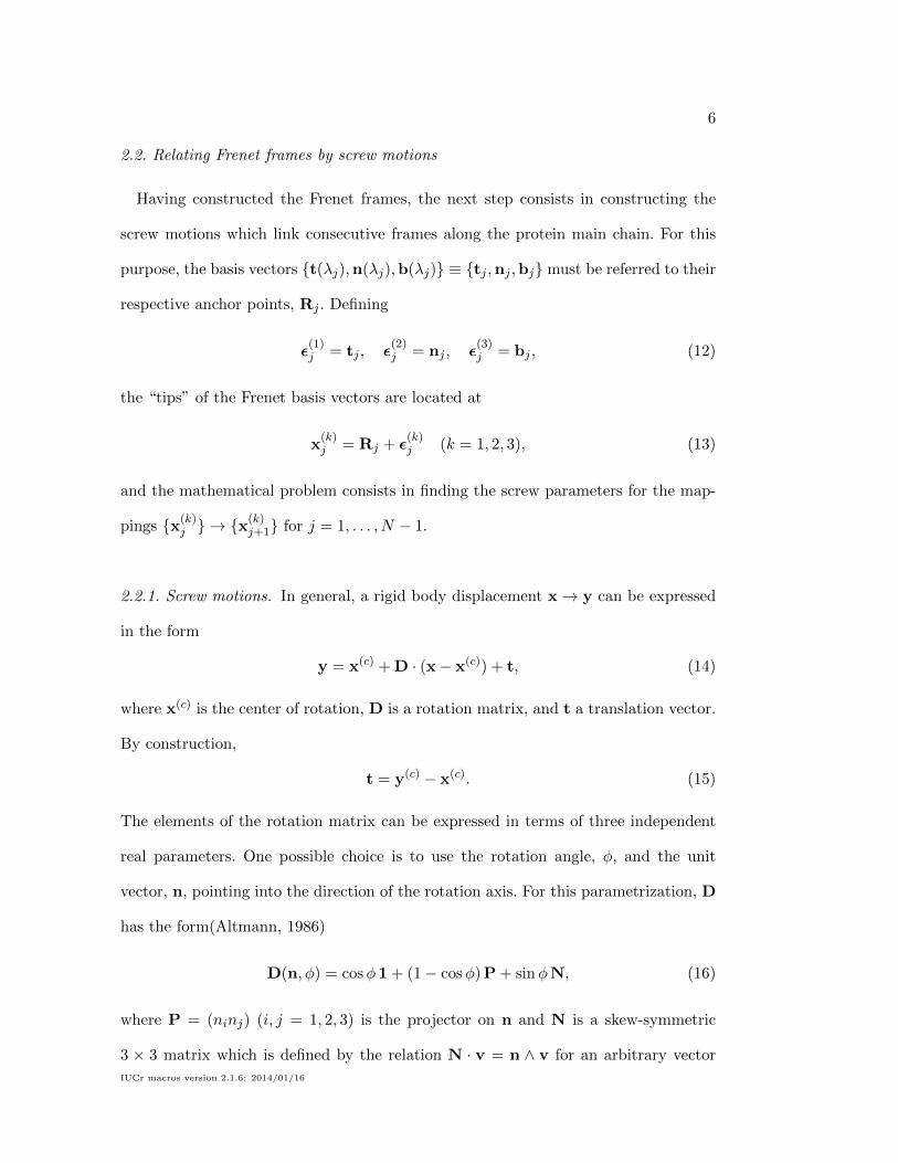
2.2. Relating Frenet frames by screw motions
Having constructed the Frenet frames, the next step consists in constructing the
screw motions which link consecutive frames along the protein main chain. For this
purpose, the basis vectors {t(λj),n(λj),b(λj)} ≡ {tj ,nj ,bj} must be referred to their
respective anchor points, Rj . Defining
ε(1)j = tj , ε
(2)j = nj , ε
(3)j = bj , (12)
the “tips” of the Frenet basis vectors are located at
x(k)j = Rj + ε
(k)j (k = 1, 2, 3), (13)
and the mathematical problem consists in finding the screw parameters for the map-
pings {x(k)j } → {x
(k)j+1} for j = 1, . . . , N − 1.
2.2.1. Screw motions. In general, a rigid body displacement x→ y can be expressed
in the form
y = x(c) + D · (x− x(c)) + t, (14)
where x(c) is the center of rotation, D is a rotation matrix, and t a translation vector.
By construction,
t = y(c) − x(c). (15)
The elements of the rotation matrix can be expressed in terms of three independent
real parameters. One possible choice is to use the rotation angle, φ, and the unit
vector, n, pointing into the direction of the rotation axis. For this parametrization, D
has the form(Altmann, 1986)
D(n, φ) = cosφ1 + (1− cosφ) P + sinφN, (16)
where P = (ninj) (i, j = 1, 2, 3) is the projector on n and N is a skew-symmetric
3 × 3 matrix which is defined by the relation N · v = n ∧ v for an arbitrary vector
IUCr macros version 2.1.6: 2014/01/16
7
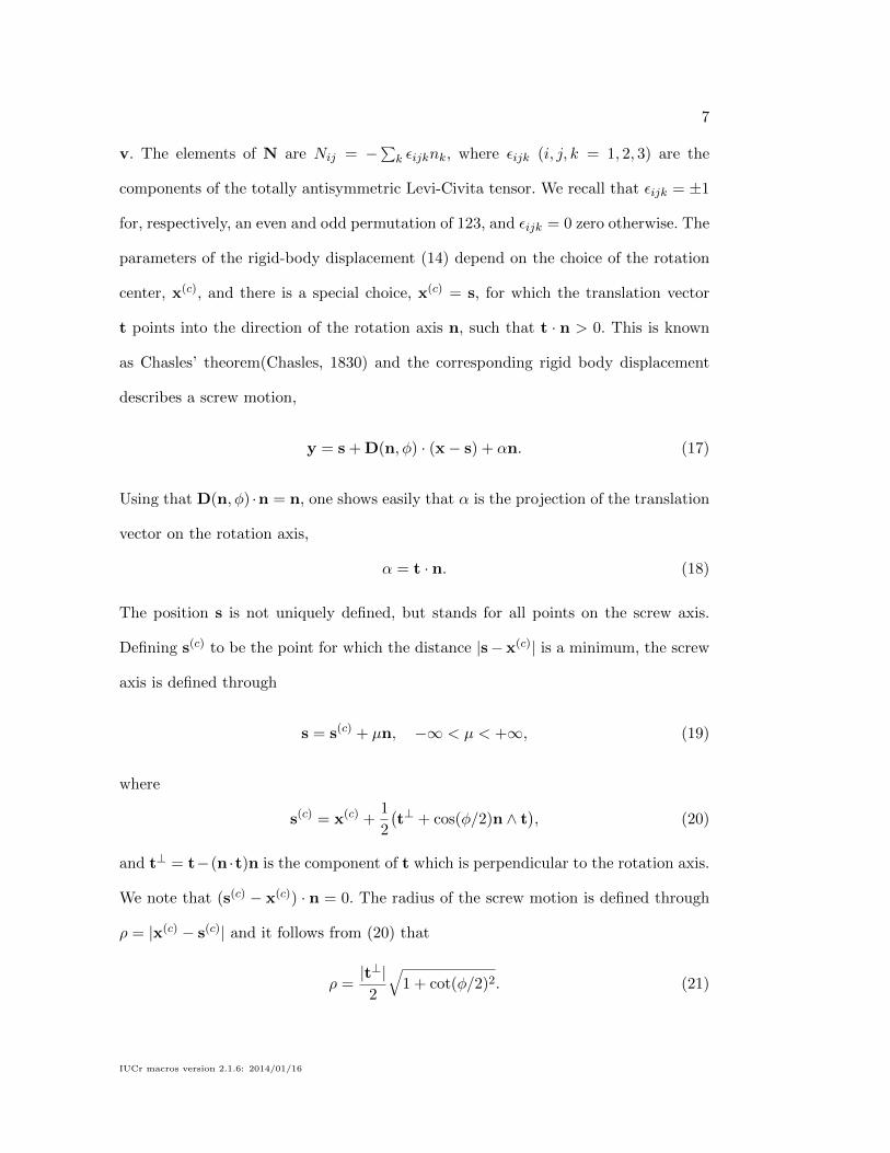
v. The elements of N are Nij = −∑k εijknk, where εijk (i, j, k = 1, 2, 3) are the
components of the totally antisymmetric Levi-Civita tensor. We recall that εijk = ±1
for, respectively, an even and odd permutation of 123, and εijk = 0 zero otherwise. The
parameters of the rigid-body displacement (14) depend on the choice of the rotation
center, x(c), and there is a special choice, x(c) = s, for which the translation vector
t points into the direction of the rotation axis n, such that t · n > 0. This is known
as Chasles’ theorem(Chasles, 1830) and the corresponding rigid body displacement
describes a screw motion,
y = s + D(n, φ) · (x− s) + αn. (17)
Using that D(n, φ) ·n = n, one shows easily that α is the projection of the translation
vector on the rotation axis,
α = t · n. (18)
The position s is not uniquely defined, but stands for all points on the screw axis.
Defining s(c) to be the point for which the distance |s−x(c)| is a minimum, the screw
axis is defined through
s = s(c) + µn, −∞ < µ < +∞, (19)
where
s(c) = x(c) +1
2
(t⊥ + cos(φ/2)n ∧ t
), (20)
and t⊥ = t−(n ·t)n is the component of t which is perpendicular to the rotation axis.
We note that (s(c) − x(c)) · n = 0. The radius of the screw motion is defined through
ρ = |x(c) − s(c)| and it follows from (20) that
ρ =|t⊥|
2
√1 + cot(φ/2)2. (21)
IUCr macros version 2.1.6: 2014/01/16
8
2.2.2. Determining the screw parameters. Assuming that the Frenet frames at the
Cα-positions have been constructed, the fold of a protein is defined by the sequence
of screw motions x(k)j → x
(k)j+1, where
x(k)j+1 = s
(c)j + D(nj , φj) · (x(k)
j − s(c)j ) + αjnj , (22)
for j = 1, . . . , n − 1 and k = 1, 2, 3. The corresponding parameters are computed as
follows:
1. Determine the translation vectors
tj = Rj+1 −Rj . (23)
2. Perform a rotational least squares fit(Kneller, 1991) {ε(k)j } → {ε(k)j+1} by mini-
mizing the target function
m(Qj) =3∑
k=1
∣∣∣ε(k)j+1 −D(Qj) · ε(k)j∣∣∣2 (24)
with respect to four quaternion parameters, Q = {q0, q1, q2, q3}, which
parametrize the rotation matrix according to
D(Q) =
q20 + q21 − q22 − q23 2 (q1q2 − q0q3) 2 (q0q2 + q1q3)2 (q1q2 + q0q3) q20 − q21 + q22 − q23 −2 (q0q1 − q2q3)−2 (q0q2 − q1q3) 2 (q0q1 + q2q3) q20 − q21 − q22 + q23
. (25)
The quaternion parameters are normalized such that q20 +q21 +q22 +q23 = 1, which
leaves three free parameters describing the rotation. We note here only that the
minimization of (24) leads to an eigenvector problem for the optimal quaternion,
which can be efficiently solved by standard linear algebra routines, and that
the corresponding eigenvalue is the squared superposition error (Kneller, 1991).
The latter is zero for superposition of Frenet frames, since two orthonormal and
equally oriented vector sets can be perfectly superposed. It is also worthwhile
noting that the upper limit in the sum in (24) can be changed from 3 to 2, since
IUCr macros version 2.1.6: 2014/01/16
9
two linearly independent vectors with the same origin, here tj and nj , suffice to
define a rigid body.
3. Extract nj and φj from the quaternion parameters Qj . This can be easily
achieved by expoiting the relations
q0 = cos(φ/2)q1 = sin(φ/2)nxq2 = sin(φ/2)nyq3 = sin(φ/2)nz
(26)
Here and in the following the index j is dropped. Several cases have to be
considered. If√q21 + q22 + q23 > ε, where ε depends on the machine precision of
the computer being used, we compute a “tentative rotation axis”
nt =1√
q21 + q22 + q23
q1q2q3
. (27)
Then we check if t · nt ≥ 0. If this is the case we set
n = nt, (28)
φ = 2 arccos(q0). (29)
In case that t · nt < 0 we set
n = −nt, (30)
φ = 2 arccos(−q0). (31)
This corresponds to replacing Q→ −Q before evaluating n and φ according to
(28) and (29). Such a replacement is possible since the elements of D(Q) are
homogeneous functions of order two in the quaternion parameters, such that
D(Q) = D(−Q).
For the sake of completeness, we finally mention the case that√q21 + q22 + q23 ≤ ε,
which corresponds to a pure translation and cannot occur in our application to
protein backbones. In this case one would set φ = 0 and n = t/|t|.IUCr macros version 2.1.6: 2014/01/16

10
4. Using the parameters {nj , φj} and defining the positions Rj to be the rotation
centers, x(c) = Rj , compute for j = 1, . . . , N − 1
(a) the positions s(c)j on the local screw axes according to relation (20),
(b) the local helix radii according to relation (21).
2.2.3. Regularity of PSSEs. To quantify the regularity of PSSEs, we introduce the
distance measure
δ(j) =∣∣∣s(c)j + t
‖j − s
(c)j+1
∣∣∣ , j = 1, . . . , N − 2, (32)
where t‖j = n·tj . For an ideal PSSE, where all consecutive Frenet frames are related by
the same screw motion, δ(j) is strictly zero. This measure of non-ideality deviates from
the “straightness” parameter in the ScrewFit algorithm (Kneller & Calligari, 2006),
which is defined as σj = µj+1 ·µj with µj = s(c)j+1 − s
(c)j , and which defines ideality of
PSSEs through the cosine of the angle between subsequent local screw axes.
2.3. Numerical test
To test the numerical construction of Frenet frames, we consider a perfect heli-
coidal curve and compare the exact Frenet frames with the corresponding numerical
approximations. The parametric representation of the curve is
r(λ) = ρ cos(λ) e(x) + ρ sin(λ) e(y) + hλ e(z), (33)
where ρ > 0 is the radius of the helix and its pitch is p = h/2π. Fig. 4 shows the
form of the curve (33) for one complete turn (red line), setting R = 1 and h = 0.3 in
arbitrary length units. Defining the matrix F(λ) = (t(λ),n(λ),b(λ)), it follows from
(33) that
F(λ) =
− R sin(λ)√
h2+R2− cos(λ) h sin(λ)√
h2+R2
R cos(λ)√h2+R2
− sin(λ) − h cos(λ)√h2+R2
h√h2+R2
0 R√h2+R2
. (34)
IUCr macros version 2.1.6: 2014/01/16
11
Using the method described in Section 2.1, we construct numerical approximations
F(λj) of the Frenet bases (34) at N = 11 equidistant sampling points, Rj , which are
shown as red dots in Fig. 4. From these Frenet bases we construct the axis points s(c)j
(blue dots), which are shown together with the exact screw axis (blue line). For the
first and the last axis point one notices a visible offset from the latter. We quantify
the error of the numerically computed Frenet bases, F(λj), as
ε(j) =√
tr {∆(j)T ·∆(j)}, (35)
where
∆(j) = F(λj)T · F(λj)− 1. (36)
For a perfect overlap of F(λj) and F(λj) one should have F(λj)T · F(λj) = 1, such
that ε(j) = 0. We note that ε(j) is the Frobenius norm (Golub & van Loan, 1996)
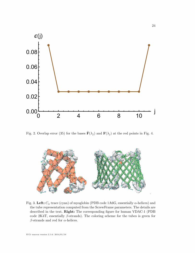
of ∆(j). Fig. 2 shows ε(j) corresponding to the Frenet basis in Fig. 4 and confirms
the slight offset of the first and last axis point from the ideal screw axis.
3. Applications
We will now consider four applications of the coarse-grained protein model described
above, which will be referred to as ScrewFrame in the following.
1. The first application concerns the construction of a tube model for two proteins
whose secondary structure elements are, respectively, essentially α-helices and
β-strands.
2. In the second application, we explore the stability of the most important
ScrewFrame parameters, ρ and δ, under perturbations of the protein structure.
3. The third application is a comparative study of ScrewFrame and DSSP for sec-
ondary structure assignment. We provide the comparison with the de facto stan-
dard DSSP as a proof of validity of our approach.
IUCr macros version 2.1.6: 2014/01/16
12
4. The fourth application is devoted to a secondary structure analysis of all protein
structures in the RSCB Protein Data Bank for which only the positions of the
Cα-atoms are known.
3.1. Tube representation of a protein
As a first application we present a ScrewFrame analysis for myoglobin, an oxygen-
binding globular protein in muscular tissues which contains essentially α-helices (PDB
code 1A6G), and for the integral human membrane protein VDAC-1, whose predomi-
nant PSSEs are β-strands (PDB code 2K4T). The upper and lower panels of Figure (3)
show tube models for the respective proteins which have been constructed from the
ScrewFrame parameters. The tube is a succession of cylinders whose radii are defined
by the ScrewFrame parameter ρ (see Eq. (21)), which describes the radius of the screw
motion linking consecutive Frenet frames. The axis of each cylinder is the local screw
axis and its height is the distance between two consecutive screw motion centers s(c)j
and s(c)j+1 (see Eq. (20)) on that axis. By definition, the Cα-atoms are on the surface
of the tube. As in the original ScrewFit algorithm, the screw radius allows for a dis-
crimination of different types of PSSEs (see Table 1) and the tube is colored red to
indicate α-helices and green for β-strands. The protein main axis is the concatenation
of all local screw axes and it plays the same role as the “overall protein axis” in the
P-Curve algorithm (Sklenar et al., 1989), although its construction is different. We
provide the tube models for these two proteins as supplementary material in the form
of BILD files for the molecular visualization program Chimera.(Pettersen et al., 2004)
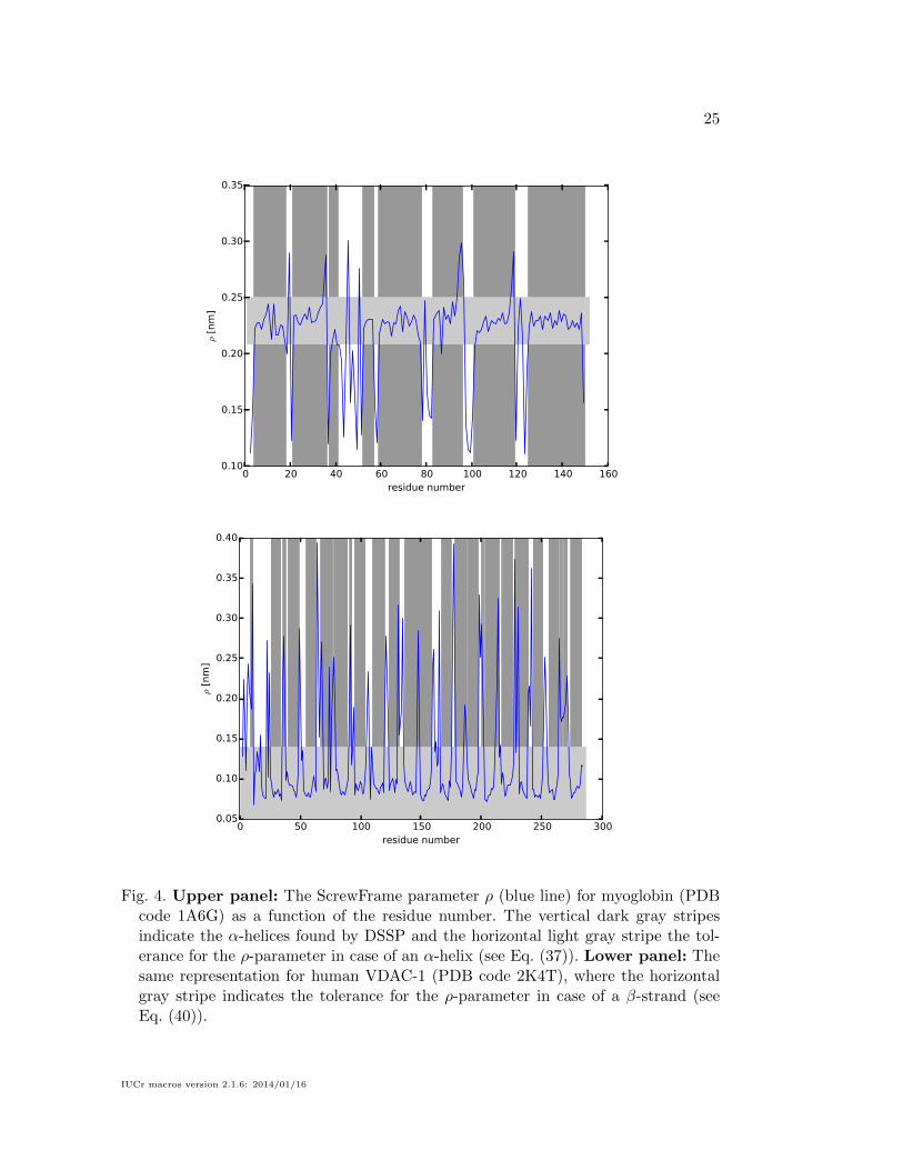
The upper and lower panels of Fig. 4 display, respectively, the parameter ρ for
myoglobin and VDAC-1 as a function of the residue index (blue line). For comparison
we also show the α-helices found by DSSP, which are indicated by the vertical stripes
in dark gray. The horizontal stripes in light gray indicate the tolerance interval for
IUCr macros version 2.1.6: 2014/01/16

13
the ρ-parameter for α-helices and β-strands, respectively, whose definition will be
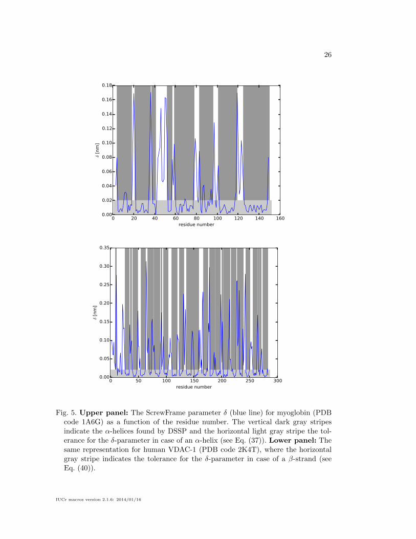
described in the following section. Fig. 5 shows the corresponding regularity measure
δ (see Eq. (32)) for myoglobin and VDAC-1 (upper and lower panel, respectively)
which plays an important role in the attribution of secondary structure elements that
will be discussed in the following section.
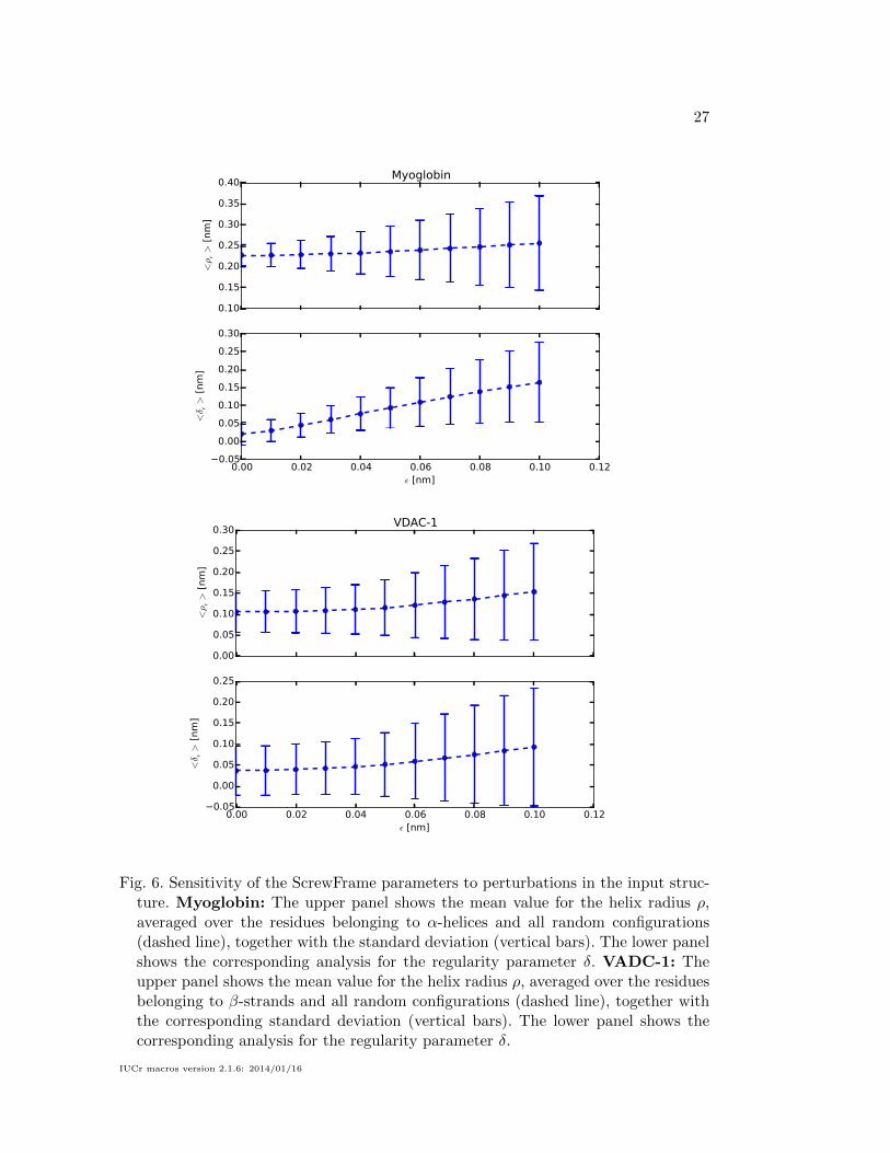
3.2. Perturbation analysis
In view of the application of our approach to low-resolution data, it is interesting to
explore the influence of perturbations in the Cα-positions on the resulting ScrewFrame
parameters. We limit ourselves to the parameters ρ and δ, which are the most impor-
tant ones for characterizing the secondary structure of a protein. As examples we
consider the PDB structures 1A6G for myoglobin and 2K4T for the VDAC-1 protein,
which were treated in the previous section. The Cartesian coordinates of all Cα-atoms
are shifted by random numbers which are drawn from a normal distribution with zero
mean and a prescribed width ε. For the latter we chose 10 values, increasing from
0.01 to 0.1 nm in steps of 0.01 nm, and for each value of ε we generate 1000 random
configurations. Figure 6 displays the results of the perturbation analysis for myoglobin
(upper two panels) and VDAC-1 (lower two panels). In both cases we show
1. the mean value for the helix radius ρ, averaged over all residues belonging to
the respective dominant motive (α-helices in case of myoglobin and β-strands
in case of VDAC-1) and all random configurations (dashed line), together with
the corresponding standard deviation (vertical bars).
2. the corresponding analysis for he regularity parameter δ.
The results show that ρ is a robust parameter, which increases slowly with increas-
ing noise, whereas δ reacts much stronger. It is indeed important for ρ to be robust,
because we use it to distinguish between different types of secondary structure ele-
IUCr macros version 2.1.6: 2014/01/16
14
ments. The role of δ is quite different: it is a quality parameter that measures the reg-
ularity of the protein fold, and it is used to distinguish “good” from “bad” secondary-
structure elements. It is thus to be expected that δ should increase for less well-defined
input structures. We expect this dependence to become useful in structure refinement
applications, where a restraint on δ can be used to enforcee well-defined secondary
structure elements.
3.3. Analysis of the ASTRAL database
In order to compare our Cα based helicoidal analysis with the original ScrewFit
method based on peptide planes (Kneller & Calligari, 2006; Calligari & Kneller, 2012),
we applied both methods to the “all α and “all β” categories of the ASTRAL subset
of the SCOPe database (Fox et al., 2013), using the ASTRAL SCOPe 2.04 subset
with less than 40% sequence identity. In order to be able to work efficiently with
such a large collection of protein structures, we constructed an ActivePaper (Hinsen,
2014a) containing the structures of the ASTRAL entries in MOSAIC format (Hinsen,
2014c). This file is available for download (Hinsen, 2014b). In addition to the ASTRAL
database of real protein structures, we use ideal secondary-structure elements (α-helix,
π-helix, 3− 10-helix, parallel and anti-parallel β-strands) for polyalanine, which were
constructed using the program Chimera (Pettersen et al., 2004).
We also compare to DSSP secondary structure assignments for this database, using
our own implementation of the DSSP algorithm which follows the description in the
original publication (Kabsch & Sander, 1983) but, like the current version 2 of the
DSSP software (Hekkelman, 2013), computes an ideal position for the backbone hydro-
gen positions instead of using experimental values, even if the latter are available.
As a first step, we compute ScrewFit and ScrewFrame parameters for all structures
in the all-α and all-β subsets of the ASTRAL database. In order to avoid inaccu-
IUCr macros version 2.1.6: 2014/01/16
15
racies introduced by the third-order approximations given by Eqs. (8)–(11), we do
not compute Frenet frames for the first and last residue of each chain. For structures
with missing residues, we compute the parameters for each continuous chain seg-
ment separately. Since the input structures are dominated by α-helices and β-strands,
respectively, we expect the distribution of our parameters to show clear peaks that
correspond to these secondary structure elements.
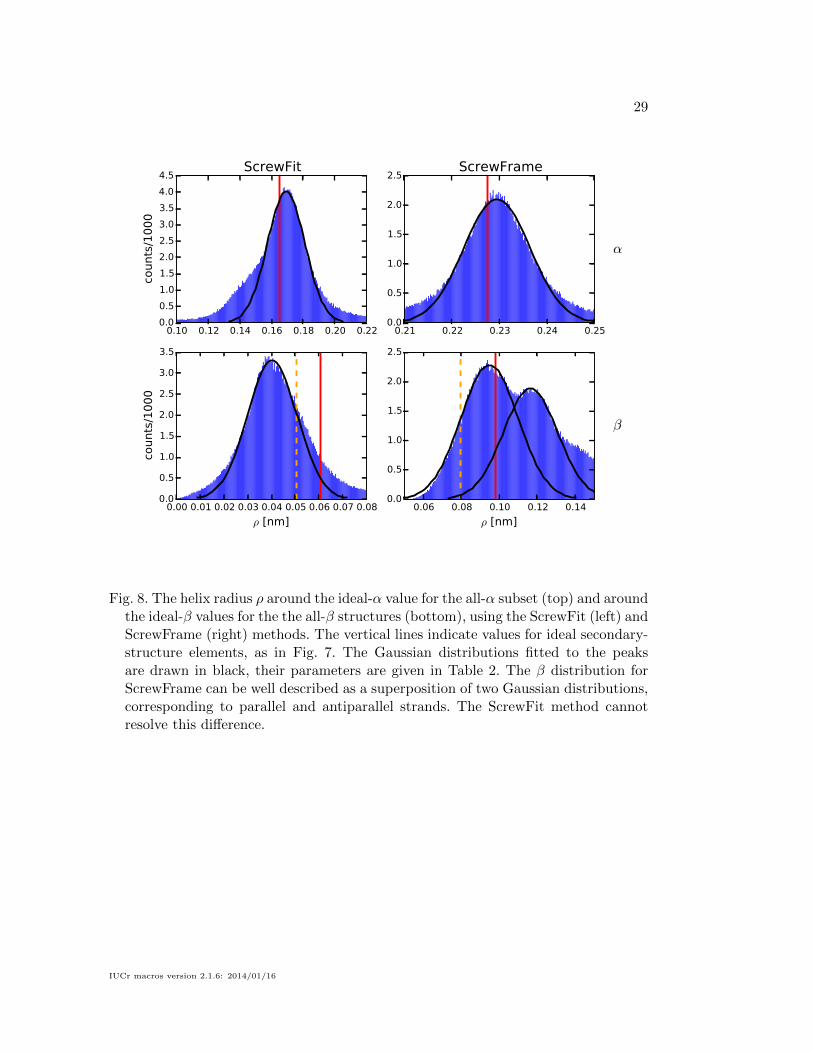
The most important helix parameter for secondary structure description is the helix
radius ρ, whose distribution in the ASTRAL database is shown in Fig. 7. The ver-
tical lines show for comparison the values for ideal α-helices and β-strands. For the
β-strands, the red drawn-out lines stand for parallel and the orange dashed lines for
antiparallel strands. A more detailed view is given in Fig. 8, which shows only the
region around the dominant peak for each histogram, together with Gaussian distri-
butions fitted to the peaks. The peaks are rather well described by a Gaussian, and
the ScrewFrame method even allows to resolve the difference between parallel and
antiparallel β-strands.
Whereas the average ρ value for α-helices is close to the value for an ideal helix,
this is not the case at all for β-strands. This can be understood by looking at the
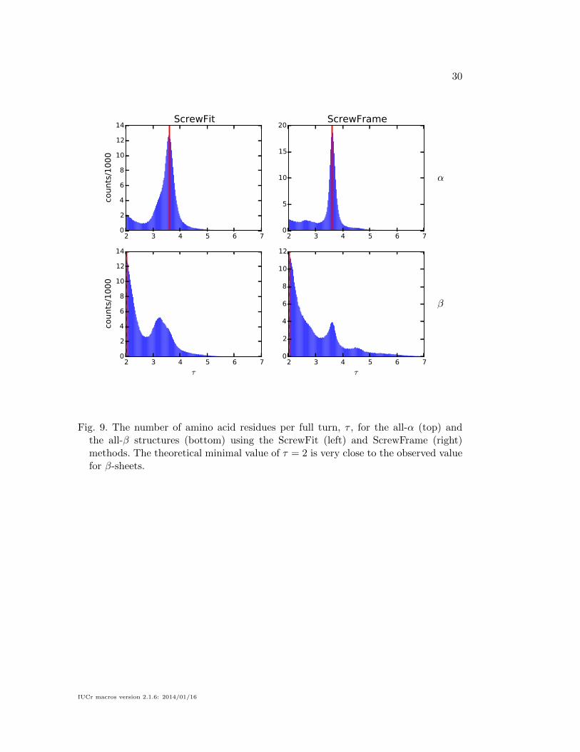
distribution of the number of amino acids per full turn, τ , shown in Fig. 9. Since
the rotation angle is by definition in the interval [−π . . . π], the minimal value of τ
is 2. This is also the value that describes an ideal β-strand, which is a flat structure.
Any deviation from the ideal β-strand has a larger τ , and because ρ and τ are not
independent (the length of the curve arc linking two neighboring Cα atoms is nearly
constant), the deviation in ρ from the ideal value is asymmetric as well.
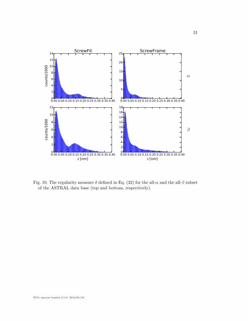
The regularity measure δ, defined in Eq. (32), is shown in Fig. 10. It shows that
the ScrewFrame secondary structure elements are more regular than those identified
by ScrewFit, in particular for structures dominated by α-helices. We do not show
IUCr macros version 2.1.6: 2014/01/16
16
here the distributions of the other parameters defined in the initial ScrewFit publica-
tion (Kneller & Calligari, 2006), but they are included in the electronic supplementary
material. We note that the parameter distributions are in general narrower and thus
better defined for ScrewFrame than for ScrewFit. We attribute this fact to fluctuations
in the orientations of the peptide plans that have no impact on the Cα geometry.
We use the Gaussian distributions shown in Fig. 8 as the basis for defining
secondary-structure elements. We define an α-helix as a sequence of at least four
consecutive Cα atoms whose screw transformations satisfy
|ρ− µρ|σρ
< 3 (37)
δ < 0.02 nm (38)
where µρ and σρ are the mean value and standard deviation of the Gaussian distri-
bution for the α peak in Fig. 8. The numerical values of these parameters are shown
in Table 2. We define a β-strand as a segment of consecutive Cα atoms whose screw
transformations satisfy
min
(|ρ− µ(1)ρ |σ(1)ρ
,|ρ− µ(2)ρ |σ(2)ρ
)< 1 (39)
δ < 0.08 nm (40)
where µ(1/2)ρ and σ
(1/2)ρ are the mean values and standard deviations of the Gaussian
distributions for the parallel and antiparallel β peaks in Fig. 8. The numerical param-
eters in these definitions were chosen to make our definitions match the secondary
structure assignments made by the DSSP method.
There is a fundamental difference between our approach and the DSSP method
for defining β-strands. The ScrewFrame approach looks for a regular structure along
the peptide chain, whereas the DSSP method identifies hydrogen bonds between the
strands that make up a β-sheet. ScrewFrame thus finds individual strands, which can
be paired up to identify sheets in a separate step. A strand must consist of at least three
IUCr macros version 2.1.6: 2014/01/16

17
consecutive residues in order to be considered regular; in fact, the regularity measure
δ is defined in terms of the difference of two consecutive screw transformations, each
of which connects two residues. DSSP needs to look at two strands simultaneously in
order to identify β structures, but has no minimal length condition and in fact admits
β-sheets as mall as a single h-bonded residue pair. For practically relevant β-sheets in
real protein structures, these differences are, however, not important, but they must
be understood for interpreting the following comparison between the two methods.
A one-to-one comparison of secondary structure elements from two different assign-
ment methods is not of particular interest, because an exact match is the exception
rather than the rule. The inherent fuziness of secondary structure definitions leads to
arbitrary choices and thus inevitable differences. The most frequent deviation between
two assignments is the end points of secondary structure elements, where a difference
of one or two residues is common and acceptable. Another frequent deviation concerns
deformed secondary structure elements, which one method may identify as a single
element whereas another one recognizes it as multiple distinct elements.
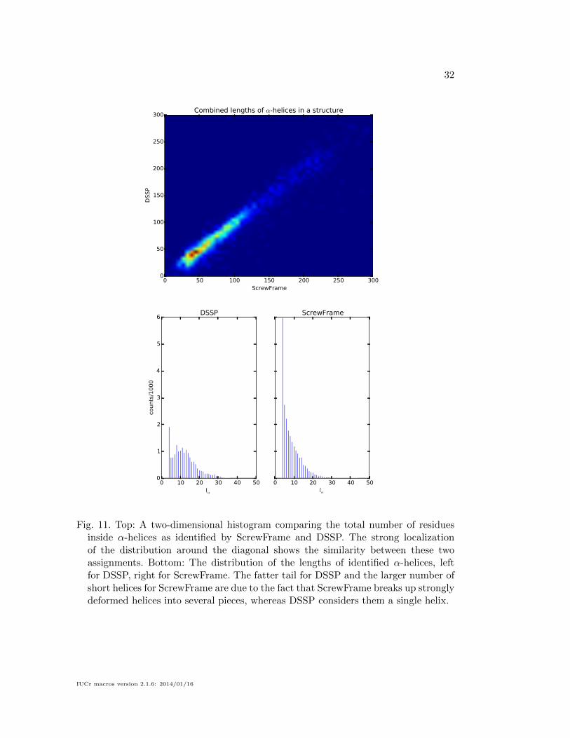
We therefore chose a statistical comparison to compare the ScrewFrame results
to those of DSSP, which is shown in Figs. 11 for α-helices and 12 for β-strands. We
consider two quantities: (1) the total number of residues of a given structure which are
inside a recognized secondary-structure element, and (2) the length of each individual
secondary-structure element. We compute the first quantity for both methods and
show their joint distribution (upper plot in the two figures). For the vast majority of
structures, the two residue counts are close to equal, which means that neither method
yields systematically more or longer secondary-structure elements than the other. The
lower plots show the distributions of the lengths of individual secondary-structure
elements. For α-helices, DSSP has a fatter tail (helices of length 20 or more), whereas
ScrewFrame identifies a larger number of short helices. The reason for these differences
IUCr macros version 2.1.6: 2014/01/16

18
is that ScrewFrame tends to split up kinked helices which DSSP identifies as single
units. For β-strands, we notice that DSSP identifies many more very short elements.
This is due to the different definitions: a single β-type hydrogen bond is sufficient to
define a β-sheet in DSSP, but ScrewFrame requires at least three consecutive residues
to identify any regular structure.
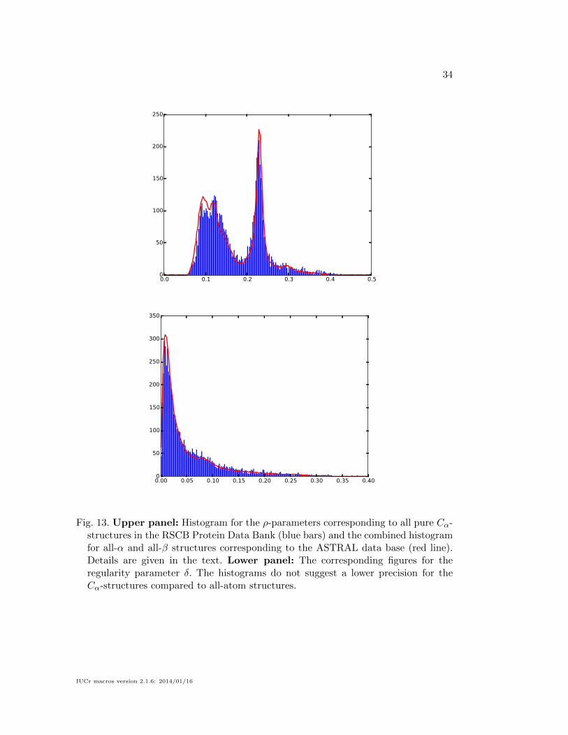
3.4. Analysis of Cα-structures in the PDB
The Protein Data Bank contains at this time 595 entries marked as “CA
ATOMS ONLY”, which correspond to low-resolution X-ray crystallography or electron
microscopy data. Secondary-structure assignment methods such as DSSP, which are
based on an analysis of hydrogen bond networks, cannot be applied to these entries.
The low resolution of the experimental data underlying these structures raises the
question whether our approach can still identify secondary structures reliably. The Cα
positions could be less precise, leading to an increased uncertainty in the ScrewFrame
parameters which we compute from them.
To investigate this question, we have computed histograms for the ScrewFrame
parameters for this set of structures, in the same way as we have described above
for the ASTRAL database. These histograms are shown in Fig 13. The red lines
show the distributions for the ASTRAL database for comparison. Since the latter are
for predominantly α- or β-containing structures, whereas the Cα-only PDB entries
contain a mixture of all kinds of structures, we must compare to a weighted sum
of the histograms of the two ASTRAL categories. The relative weights have been
determined empirically: the red lines in the figure correspond to the sum of 0.0067
times the α histogram (upper-right plots in Figs. 7 and 10) and 0.01 times the β
histogram (lower-right plots in Figs. 7 and 10).
The excellent agreement of the histograms suggests that there is no difference in
IUCr macros version 2.1.6: 2014/01/16

19
the uncertainty of the ScrewFrame parameters between PDB entries for low-resolution
data and PDB entries in general. A possible explanation is that there is already no
increased uncertainty in the Cα positions. Many of the Cα-only structures in the
PDB have at least partly been obtained by rigid fitting of all-atom protein structures
obtained from higher-resolution experiments. The relative positions of the Cα atoms
are therefore no less precise than in an all-atom structure. Unfortunately the infor-
mation provided in the PDB entries (and even in the accompanying articles) is not
sufficient to identify those parts of any given structure that were constructed with less
precise methods, making a more detailed investigation of this question impossible.
4. Conclusion and Outlook
We have presented a generalization of the ScrewFit method for protein structure
assignment and description, which uses only the positions of the Cα-atoms along the
protein backbone. As in the ScrewFit approach, the global protein fold is described as
a succession of screw motions relating consecutive recurrent motifs along the protein
backbone, but the “motifs” are here the tripods (planes) formed by the three (two)
orthonormal vectors of the local Frenet bases to the Cα space curve. Despite the fact
that ScrewFrame uses less information than ScrewFit, all standard PSSEs are recog-
nized on the basis of thresholds for the local screw radii and a suitably defined regular-
ity measure. ScrewFrame even permits to distinguish between parallel and antiparallel
β-strands, which the classical ScrewFit method fails to do. A thorough comparison
with the commonly used DSSP method on the assignment of PSSEs in the ASTRAL
database shows that both methods yield very similar results for the total amount of
PSSEs. ScrewFrame tends, however, to break long helices into smaller pieces, such that
the length distribution of PSSEs is different. Due to the minimalistic character of the
geometrical model for protein folds, the evaluation of the ScrewFrame model parame-
IUCr macros version 2.1.6: 2014/01/16
20
ters is very efficient. This allows for working with protein structure databases and for
analyzing simulated molecular dynamics trajectories of proteins. We have also shown
that ScrewFrame is robust with respect to perturbations of the input structures. The
local helix radius varies only little, whereas the regularity parameter δ increases visi-
bly. This is exactly what is needed in structure refinement of low resolution data where
thresholds on δ may be used to enforce more or less ideal PSSEs. ScrewFrame may
also be used a starting point for the development of minimalistic models for protein
structure and dynamics, similar to the wormlike chain model (Doi & Edwards, 1986),
which has been successfully applied to DNA (Marko & Siggia, 1995). Our method
may also be used to analyze dynamical processes, such as the folding and unfolding
of peptides (Spampinato & Maccari, 2014) and it can describe the fold of intrinsically
disordered proteins.
An ActivePaper (Hinsen, 2014a) containing all the software, input datasets, and
results from this study is available as supplementary material. The datasets can be
inspected with any HDF5-compatible software, e.g. the free HDFView.(The HDF
Group, 2013) Running the programs on different input data requires the ActivePaper
software (Hinsen, 2014a).
References
Altmann, S. (1986). Rotations, Quaternions, and Double Groups. Oxford: Clarendon Press.
Andersen, C. A. F., Palmer, A. G., Brunak, S. & Rost, B. (2002). Structure, 10(2), 175–184.
Calligari, P. A. & Kneller, G. R. (2012). Acta Crystallogr D, 68(12), 1690–1693.
Chandonia, J.-M., Hon, G., Walker, N. S., Lo Conte, L., Koehl, P., Levitt, M. & Brenner,S. E. (2004). Nucleic Acids Research, 32(Database issue), D189–92.
Chasles, M. (1830). Bulletin des Sciences Mathematiques, Astronomiques, Physiques et Chim-iques, 14, 321–326.
Doi, M. & Edwards, S. (1986). The theory of Polymer Dynamics. New York: Oxford UniversityPress.
Dupuis, F., Sadoc, J.-F. & Mornon, J.-P. (2004). Proteins, 55(3), 519–528.
Fox, N. K., Brenner, S. E. & Chandonia, J. M. (2013). Nucleic Acids Research, 42(D1),D304–D309.
Frishman, D. & Argos, P. (1995). Proteins, 23(4), 566–579.
Golub, G. & van Loan, C. (1996). Matrix Computations. The John Hopkins University Press.
IUCr macros version 2.1.6: 2014/01/16
21
Grimes, J. M., Fuller, S. D. & Stuart, D. I. (1999). Acta Crystallogr D, 55(10), 1742–1749.
Hekkelman, M., (2013). DSSP 2.2.1. http://swift.cmbi.ru.nl/gv/dssp/.
Hinsen, K., (2014a). ActivePapers. http://www.activepapers.org/.
Hinsen, K., (2014b). ASTRAL-SCOPe subset 2.04 in ActivePapers format.URL: http://dx.doi.org/10.5281/zenodo.11086
Hinsen, K. (2014c). Journal of chemical information and modeling, 54(1), 131–137.
Hu, S., Lundgren, M. & Niemi, A. J. (2011). Phys Rev E, 83(6), 061908.
Kabsch, W. & Sander, C. (1983). Biopolymers, 22(12), 2577–2637.
Kirchmair, J., Markt, P., Distinto, S., Schuster, D., Spitzer, G., Liedl, K., Langer, T. & Wolber,G. (2008). J. Med. Chem, 51(22), 7021–7040.
Kneller, G. R. (1991). Mol Simulat, 7(1), 113–119.
Kneller, G. R. & Calligari, P. (2006). Acta Crystallogr D, 62(3), 302–311.
Labesse, G., Colloc’h, N., Pothier, J. & Mornon, J.-P. (1997). Computer applications in thebiosciences: CABIOS, 13(3), 291–295.
Levitt, M. & Greer, J. (1977). J Mol Biol, 114(2), 181–239.
Marabini, R., Macias, J. R., Vargas, J., Quintana, A., Sorzano, C. O. S. & Carazo, J. M.(2013). Acta Crystallogr D, 69(5), 695–700.
Marko, J. F. & Siggia, E. D. (1995). Macromolecules, 28(26), 8759–8770.
Park, S.-Y., Yoo, M.-J., Shin, J.-M. & Cho, K.-H. (2011). BMB Reports, 44(2), 118–122.
Pauling, L. & Corey, R. B. (1951). P Natl Acad Sci Usa, 37(11), 729.
Pauling, L., Corey, R. B. & Branson, H. R. (1951). P Natl Acad Sci Usa, 37(4), 205–211.
Pettersen, E. F., Goddard, T. D., Huang, C. C., Couch, G. S., Greenblatt, D. M., Meng, E. C.& Ferrin, T. E. (2004). J Comput Chem, 25(13), 1605–1612.
Sklenar, H., Etchebest, C. & Lavery, R. (1989). Proteins, 6(1), 46–60.
Spampinato, G. & Maccari, G. (2014). J. Chem. Theory Comput, 10, 38853895.
The HDF Group, (2013). HDFView. http://www.hdfgroup.org/hdf-java-html/hdfview/.
Tozzini, V. (2005). Curr. Opin. Struct. Biol. 15(2), 144–150.
Wolfram Research Inc. (2014). Mathematica. Version 10.0. Champaign, Illinois, USA: WolframResearch Inc.
IUCr macros version 2.1.6: 2014/01/16
22
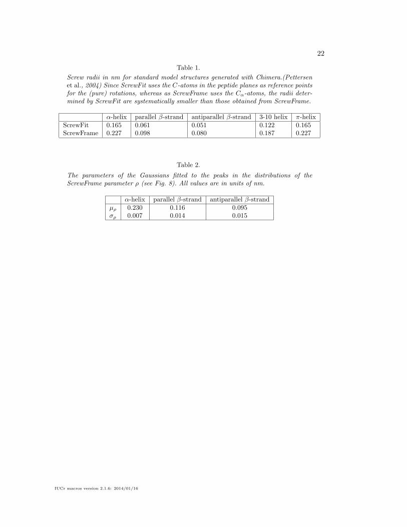
Table 1.
Screw radii in nm for standard model structures generated with Chimera.(Pettersenet al., 2004) Since ScrewFit uses the C-atoms in the peptide planes as reference pointsfor the (pure) rotations, whereas as ScrewFrame uses the Cα-atoms, the radii deter-mined by ScrewFit are systematically smaller than those obtained from ScrewFrame.
α-helix parallel β-strand antiparallel β-strand 3-10 helix π-helixScrewFit 0.165 0.061 0.051 0.122 0.165ScrewFrame 0.227 0.098 0.080 0.187 0.227
Table 2.
The parameters of the Gaussians fitted to the peaks in the distributions of theScrewFrame parameter ρ (see Fig. 8). All values are in units of nm.
α-helix parallel β-strand antiparallel β-strandµρ 0.230 0.116 0.095σρ 0.007 0.014 0.015
IUCr macros version 2.1.6: 2014/01/16

23
t
n
b
Fig. 1. Frenet frame {t,n,b} at one point of the helicoidal curve defined in Eq. (33)(red solid line). Setting R = 1 and h = 0.3, the latter is shown for one turn,together with N = 11 equidistantly spaced sampling points (red points). Theblue line is the helix axis and the blue points correspond to the rotation cen-
ters s(c)j (j = 1, . . . N − 1). The figure has been produced with the Mathematica
software (Wolfram Research Inc., 2014).
IUCr macros version 2.1.6: 2014/01/16
24
0 2 4 6 8 10j0.00
0.02
0.04
0.06
0.08
ϵ(j)
Fig. 2. Overlap error (35) for the bases F(λj) and F(λj) at the red points in Fig. 4.
.
Fig. 3. Left: Cα trace (cyan) of myoglobin (PDB code 1A6G, essentially α-helices) andthe tube representation computed from the ScrewFrame parameters. The details aredescribed in the text. Right: The corresponding figure for human VDAC-1 (PDBcode 2K4T, essentially β-strands). The coloring scheme for the tubes is green forβ-strands and red for α-helices.
IUCr macros version 2.1.6: 2014/01/16
25
0 20 40 60 80 100 120 140 160residue number
0.10
0.15
0.20
0.25
0.30
0.35
ρ [
nm
]
0 50 100 150 200 250 300residue number
0.05
0.10
0.15
0.20
0.25
0.30
0.35
0.40
ρ [
nm
]
Fig. 4. Upper panel: The ScrewFrame parameter ρ (blue line) for myoglobin (PDBcode 1A6G) as a function of the residue number. The vertical dark gray stripesindicate the α-helices found by DSSP and the horizontal light gray stripe the tol-erance for the ρ-parameter in case of an α-helix (see Eq. (37)). Lower panel: Thesame representation for human VDAC-1 (PDB code 2K4T), where the horizontalgray stripe indicates the tolerance for the ρ-parameter in case of a β-strand (seeEq. (40)).
IUCr macros version 2.1.6: 2014/01/16
26
0 20 40 60 80 100 120 140 160residue number
0.00
0.02
0.04
0.06
0.08
0.10
0.12
0.14
0.16
0.18
δ [n
m]
0 50 100 150 200 250 300residue number
0.00
0.05
0.10
0.15
0.20
0.25
0.30
0.35
δ [n
m]
Fig. 5. Upper panel: The ScrewFrame parameter δ (blue line) for myoglobin (PDBcode 1A6G) as a function of the residue number. The vertical dark gray stripesindicate the α-helices found by DSSP and the horizontal light gray stripe the tol-erance for the δ-parameter in case of an α-helix (see Eq. (37)). Lower panel: Thesame representation for human VDAC-1 (PDB code 2K4T), where the horizontalgray stripe indicates the tolerance for the δ-parameter in case of a β-strand (seeEq. (40)).
IUCr macros version 2.1.6: 2014/01/16
27
0.10
0.15
0.20
0.25
0.30
0.35
0.40
<ρε>
[nm
]
Myoglobin
0.00 0.02 0.04 0.06 0.08 0.10 0.12ε [nm]
0.05
0.00
0.05
0.10
0.15
0.20
0.25
0.30
<δ ε>
[nm
]
0.00
0.05
0.10
0.15
0.20
0.25
0.30
<ρε>
[nm
]
VDAC-1
0.00 0.02 0.04 0.06 0.08 0.10 0.12ε [nm]
0.05
0.00
0.05
0.10
0.15
0.20
0.25
<δ ε>
[nm
]
Fig. 6. Sensitivity of the ScrewFrame parameters to perturbations in the input struc-ture. Myoglobin: The upper panel shows the mean value for the helix radius ρ,averaged over the residues belonging to α-helices and all random configurations(dashed line), together with the standard deviation (vertical bars). The lower panelshows the corresponding analysis for the regularity parameter δ. VADC-1: Theupper panel shows the mean value for the helix radius ρ, averaged over the residuesbelonging to β-strands and all random configurations (dashed line), together withthe corresponding standard deviation (vertical bars). The lower panel shows thecorresponding analysis for the regularity parameter δ.
IUCr macros version 2.1.6: 2014/01/16

28
0.0 0.1 0.2 0.3 0.4 0.50
2
4
6
8
10
12
14
16
18
counts
/1000
ScrewFit
0.0 0.1 0.2 0.3 0.4 0.50
5
10
15
20
25
30
α
ScrewFrame
0.0 0.1 0.2 0.3 0.4 0.5
ρ [nm]
0
5
10
15
20
25
counts
/1000
0.0 0.1 0.2 0.3 0.4 0.5
ρ [nm]
0
2
4
6
8
10
12
β
Fig. 7. The helix radius ρ for the all-α (top) and the all-β structures (bottom), usingthe ScrewFit (left) and ScrewFrame (right) methods. Note that the ScrewFit radiusis based on the C-atoms, whereas the ScrewFrame radius corresponds to the Cα-atoms, which explains the different values. The vertical lines indicate the values forideal secondary-structure elements. For β-strands, there are two ideal values, onefor parallel (red, drawn-out) and one for antiparallel (orange, dashed) strands.
IUCr macros version 2.1.6: 2014/01/16
29
0.10 0.12 0.14 0.16 0.18 0.20 0.220.0
0.5
1.0
1.5
2.0
2.5
3.0
3.5
4.0
4.5
counts
/1000
ScrewFit
0.21 0.22 0.23 0.24 0.250.0
0.5
1.0
1.5
2.0
2.5
α
ScrewFrame
0.00 0.01 0.02 0.03 0.04 0.05 0.06 0.07 0.08
ρ [nm]
0.0
0.5
1.0
1.5
2.0
2.5
3.0
3.5
counts
/1000
0.06 0.08 0.10 0.12 0.14
ρ [nm]
0.0
0.5
1.0
1.5
2.0
2.5
β
Fig. 8. The helix radius ρ around the ideal-α value for the all-α subset (top) and aroundthe ideal-β values for the the all-β structures (bottom), using the ScrewFit (left) andScrewFrame (right) methods. The vertical lines indicate values for ideal secondary-structure elements, as in Fig. 7. The Gaussian distributions fitted to the peaksare drawn in black, their parameters are given in Table 2. The β distribution forScrewFrame can be well described as a superposition of two Gaussian distributions,corresponding to parallel and antiparallel strands. The ScrewFit method cannotresolve this difference.
IUCr macros version 2.1.6: 2014/01/16
30
2 3 4 5 6 70
2
4
6
8
10
12
14
counts
/1000
ScrewFit
2 3 4 5 6 70
5
10
15
20
α
ScrewFrame
2 3 4 5 6 7
τ
0
2
4
6
8
10
12
14
counts
/1000
2 3 4 5 6 7
τ
0
2
4
6
8
10
12
β
Fig. 9. The number of amino acid residues per full turn, τ , for the all-α (top) andthe all-β structures (bottom) using the ScrewFit (left) and ScrewFrame (right)methods. The theoretical minimal value of τ = 2 is very close to the observed valuefor β-sheets.
IUCr macros version 2.1.6: 2014/01/16
31
0.00 0.05 0.10 0.15 0.20 0.25 0.30 0.35 0.400
2
4
6
8
10
12
14
counts
/1000
ScrewFit
0.00 0.05 0.10 0.15 0.20 0.25 0.30 0.35 0.400
5
10
15
20
25
α
ScrewFrame
0.00 0.05 0.10 0.15 0.20 0.25 0.30 0.35 0.40
δ [nm]
0
2
4
6
8
10
12
counts
/1000
0.00 0.05 0.10 0.15 0.20 0.25 0.30 0.35 0.40
δ [nm]
0
2
4
6
8
10
12
14
16
18
β
Fig. 10. The regularity measure δ defined in Eq. (32) for the all-α and the all-β subsetof the ASTRAL data base (top and bottom, respectively).
IUCr macros version 2.1.6: 2014/01/16
32
0 50 100 150 200 250 300ScrewFrame
0
50
100
150
200
250
300
DSSP
Combined lengths of α-helices in a structure
0 10 20 30 40 50lα
0
1
2
3
4
5
6
counts
/10
00
DSSP
0 10 20 30 40 50lα
ScrewFrame
Fig. 11. Top: A two-dimensional histogram comparing the total number of residuesinside α-helices as identified by ScrewFrame and DSSP. The strong localizationof the distribution around the diagonal shows the similarity between these twoassignments. Bottom: The distribution of the lengths of identified α-helices, leftfor DSSP, right for ScrewFrame. The fatter tail for DSSP and the larger number ofshort helices for ScrewFrame are due to the fact that ScrewFrame breaks up stronglydeformed helices into several pieces, whereas DSSP considers them a single helix.
IUCr macros version 2.1.6: 2014/01/16

33
0 50 100 150 200 250 300ScrewFrame
0
50
100
150
200
250
300
DSSP
Combined lengths of β-strands in a structure
0 10 20 30 40 50lβ
0
5
10
15
20
25
30
35
40
counts
/10
00
DSSP
0 10 20 30 40 50lβ
ScrewFrame
Fig. 12. Top: A two-dimensional histogram comparing the total number of residuesinside β-strands as identified by ScrewFrame and DSSP. The strong localizationof the distribution around the diagonal shows the similarity between these twoassignments. Bottom: The distribution of the lengths of identified β-helices, left forDSSP, right for ScrewFrame. The peak at very short strands in the DSSP distri-bution is absent from the ScrewFrame results because ScrewFrame needs at leastthree consecutive residues to recognize a regular structure.
IUCr macros version 2.1.6: 2014/01/16
34
0.0 0.1 0.2 0.3 0.4 0.50
50
100
150
200
250
0.00 0.05 0.10 0.15 0.20 0.25 0.30 0.35 0.400
50
100
150
200
250
300
350
Fig. 13. Upper panel: Histogram for the ρ-parameters corresponding to all pure Cα-structures in the RSCB Protein Data Bank (blue bars) and the combined histogramfor all-α and all-β structures corresponding to the ASTRAL data base (red line).Details are given in the text. Lower panel: The corresponding figures for theregularity parameter δ. The histograms do not suggest a lower precision for theCα-structures compared to all-atom structures.
IUCr macros version 2.1.6: 2014/01/16
35
Synopsis
The paper presents a generalization of the ScrewFit method for protein secondary structuredescription and analysis (Acta Cryst. D 62, 302 (2006), Acta Cryst. D68, 1690–1693 (2012))which uses only the positions of the Cα-atoms and describes the winding of the protein mainchain as a succession of screw motions which link consecutive residue-based Frenet frames onthe discrete Cα-space curve.
IUCr macros version 2.1.6: 2014/01/16