Embed Size (px)
Citation preview

Protection for Free? The Political Economy of U.S. Tariff
Suspensions∗
Rodney D. Ludema, Georgetown University†
Anna Maria Mayda, Georgetown University and CEPR‡
Prachi Mishra, International Monetary Fund§
December 2013
Abstract
This paper studies the political influence of individual firms on Congressional decisions to suspend
tariffs on U.S. imports of intermediate goods. We develop a model of legislative bargaining in which firms
influence legislators by transmitting information about the value of protection, using verbal messages
and lobbying expenditures. We estimate our model using firm-level data on tariff suspension bills and
lobbying expenditures from 1999-2006. We find that, controlling for lobbying expenditures, an increase
in the number of import-competing firms expressing opposition to a suspension significantly reduces the
probability of that suspension being granted, suggesting that firm messages do indeed contain policy-
relevant information. We further find that lobbying expenditures by proponent and opponent firms sway
this probability in opposite directions. The effect of the number of opponents is significantly larger than
that of both opponent and proponent spending. We infer that greater information content of verbal
opposition fully accounts for its greater effectiveness relative to opponent spending and accounts for
about three quarters of its greater effectiveness relative to proponent spending, with the remaining one
quarter explained by legislative bargaining costs.
1 Introduction
With the success of the WTO in binding and reducing tariffs over the recent decades, it is tempting to
believe that the tariff schedules of WTO members are largely static between negotiating rounds. In fact,
tariff schedules are constantly being modified. In the United States, Congress regularly passes Miscellaneous
Tariff Bills (MTBs), each containing hundreds of modifications to the harmonized tariff schedule. The
∗We are grateful for the excellent research assistance of Anastasiya Denisova, Manzoor Gill, Melina Papadopoulos, JoseRomero, Natalie Tiernan, and especially Kendall Dollive. We thank Andy Berg, Mitali Das, Luca Flabbi, Gene Grossman,Giovanni Maggi, David Romer, Francesco Trebbi, and Frank Vella for invaluable advice and seminar participants at theEuropean University Institute, EIIT, the Midwest International Economics meetings, IFPRI, IMF, OECD, USITC, WorldBank, Georgetown, LSE, Paris School of Economics, Rutgers, Stanford, University of Chicago, University of Virginia, Williamand Mary and Yale for many insightful comments.
†Department of Economics and School of Foreign Service, Georgetown University, Washington, DC, 20057, USA. Email:[email protected].
‡Department of Economics and School of Foreign Service, Georgetown University, Washington, DC, 20057, USA. Email:[email protected].
§Monetary and Capital Markets Department, International Monetary Fund, Washington DC, 20431, USA. Email:[email protected].
1

European Union modifies its tariff schedule in a similar fashion every six months.1 The modifications made
under such schemes are primarily in the form of tariff “suspensions,” which eliminate MFN tariffs on specific
products for a renewable period of two to three years. Over 1400 individual suspension bills were introduced
in the U.S. Congress between 1999 and 2006, covering about 600 unique tariff lines and worth an estimated
$1.6 billion in tariff revenue, making tariff suspensions one of the nation’s largest unilateral trade policy
programs, comparable in size to the U.S. antidumping program.2 Furthermore, the process by which these
individual bills get collected into an MTB and thus become law – a formalized contest between firms seeking
to avoid paying duties on imported intermediates and firms competing against such imports – is a unique
laboratory for exploring some basic questions about the political economy of trade policy.
Several features of tariff suspensions make them ideal for studying how firms influence trade policy.
First, they are completely discretionary. Unlike practically all other trade policies, there are no international
constraints on tariff suspensions. While WTO rules tightly regulate the ability of countries to raise tariffs
above their bound rates, they do not deter countries from reducing them. This means we can reasonably
expect domestic political considerations to dominate.3 Second, they are precisely measured. Unlike coverage
ratios of non-tariff barriers, suspensions involve no measurement error. Third, we directly observe the firms
involved. Each individual bill is requested by a single importing firm (called the “proponent”) and covers
a product narrowly defined to benefit that firm. Usually, no more than a few firms produce a product
similar to the one being imported and thus might oppose the suspension. This enables us to investigate the
political economy of protection at the firm level, free from aggregation issues.4 Finally, we observe different
instruments that firms use to influence the government, specifically firm-level political spending (i.e., lobbying
expenditures and campaign contributions) and verbal messages that firms send to the government concerning
each tariff suspension. This enables us to determine which of these instruments is decisive in trade policy,
and in particular, whether information supplied by firms, independent of their political spending, has an
effect.
One of the foremost questions in the broader political economy literature is whether special interest
groups influence policy by offering money to politicians as quid pro quo5 or by strategically informing
politicians about policy consequences. Grossman and Helpman (2001) discuss both of these strategies in
depth, offering evidence for both; however, the literature remains divided. The trade literature has focused
almost exclusively on the quid pro quo channel, following Grossman and Helpman (1994), while outside of
trade, especially in the political science literature, the information channel has gained acceptance (see inter
alia Wright, 1996). The approach in the trade literature is surprising given that virtually all trade policy
1See European Union (1998).2For example, U.S. antidumping petitions from 1999 to 2006 covered only 457 separate tariff lines (authors’ calculations using
Bown (2007)). In 2007, revenue from antidumping duties was $284 million compared to $328 million lost to tariff suspensions.Gallway, Blonigen and Flynn (1999), however, argue that administrative reviews tend to suppress antidumping revenue, andafter correcting for this, put the domestic welfare impact of US antidumping duties in the range of $2-4 billion annually.Szamosszegi (2009) estimates the domestic welfare impact of tariff suspensions passed in 2009 at $3.5 billion.
3Previous work on the domestic political determinants of trade policy (e.g., Trefler, 1993; Goldberg and Maggi, 1999;Gawande and Bandyopadhyay, 2000) has used nontariff barrier (NTB) coverage ratios to measure import protection on thegrounds that NTBs are more likely to be determined unilaterally than tariffs. Gawande, Krishna and Robbins (2006) disputethis rationale, arguing, “there is no convincing evidence that all or even most NTBs are determined in a purely unilateralfashion.”
4Most previous studies, ibid, have used data at the sector level on campaign contributions by political action committees(PACs). At this level of aggregation, all sectors appear to be politically organized, in the sense of making positive politicalcontributions. This has been a major source of criticism of this line of research (see, Ederington and Minier, 2008, and Imai,Katayama and Krishna, 2013). At the firm level, this problem does not arise, and as will become evident, our empirical strategyrelies on this fact.
5We reserve the term quid pro quo for an exchange of money for policy, as discussed in Grossman and Helpman (1994, 2001).Politicians may also be disciplined by non-monetary responses to policies, such as votes, but we do not call this quid pro quo.
2
decisions involve some kind of stakeholder outreach by the government, whereby affected parties can voice
their concerns.6
The common approach in the literature to disentangling quid pro quo from information tranmission is
to distinguish between the two main types of political spending: contributions and lobbying expenditures.
Many papers find evidence of an effect of campaign contributions by political action committees (PACs) on
government policy and interpret this as evidence of a quid pro quo effect (see Snyder, 1990, Goldberg and
Maggi, 1999, Gawande and Bandyopadhyay, 2000, to name a few). Others find a similar effect of lobbying
expenditures on policy-related outcomes and interpret this as evidence of information transmission (e.g., de
Figueiredo and Silverman, 2008, Gawande, Maloney and Montes-Rojas, 2009). Survey studies documenting
the various advocacy activities of lobbyists and legal restrictions on the use of lobbying expenditures for
campaign purposes are also cited as evidence of lobbying’s informational role (see Grossman and Helpman,
2001, and de Figueiredo and Cameron, 2008). However, these distinctions ignore that PAC contributions
may also convey policy-relevant information (as in Lohmann, 1995) and that lobbying expenditures may be
fungible – there are numerous ways in which lobbyists indirectly pay off politicians, such as by promising
future employment (the “revolving door”) or facilitating fundraising.7 Thus different types of political spend-
ing do not cleanly distinguish quid pro quo from information tranmission,8 though information transmission
can take place without money. The novelty of our paper is the examination of a setting in which information
transmission – in the form of verbal messages – can be isolated from politcal spending. If messages are
effective in influencing policy, even in the absence of, or controlling for, political spending, then we have solid
evidence for an information effect.
Our dataset covers all tariff suspensions introduced in the 106th through 109th Congresses (1999-2006).
Members of Congress sponsor individual suspension bills at the request of proponent firms. These bills
are then referred to either the House Ways and Means Subcommittee on Trade or the Senate Finance
Committee, depending on where the bill was introduced, and also sent to the United States International
Trade Commission (USITC). The role of the Committees is to decide which of the suspension bills to include
in the final MTB, whereupon the MTB is passed by the full Congress by unanimous consent. Our dependent
variable is thus an indicator of whether or not the tariff suspension was included in an MTB and thus
implemented.9 The role of the USITC is to report technical information to Congress on each bill, including
the applicable tariff rate, dutiable imports, and estimated tariff revenue loss, and to conduct a survey of
domestic producers of similar products to gauge opposition to the measure. About one out of six bills in our
sample drew opposition via this mechanism.
We link the data from the USITC bill reports to a novel firm-level lobbying dataset we compiled using
information from the Center for Responsive Politics and the Senate Office of Public Records (SOPR), which
allows us to identify lobbying expenditures at the firm level by targeted policy area. We are thus able to use
lobbying expenditures that are specifically channeled towards shaping policies related to the tariff suspension
bill. This represents a significant improvement in the quality of the data relative to PAC contributions, which
6Congress regularly conducts hearings on trade policies of all kinds, most notably trade agreements up for ratification. USTRmaintains standing advisory committees and holds periodic “stakeholder” meetings that include firms, consumer groups, NGOs,etc. The USITC hears testimony from litigants in AD and CVD cases and also from downstream users of named products.
7Gawande, Krishna and Robbins (2006) discuss the fungibility of lobbying expenditures and rely on it to estimate the effectof foreign lobbying on trade policy in a quid pro quo model. Bombardini and Trebbi (2009) assume that lobbying conveysservices to politicians in a manner equivalent to contributions.
8Facchini, Mayda and Mishra (2009), Igan, Mishra and Tressel (2010), and Chin, Parsley, and Wang (2010) all reach the sameconclusion and thus examine the impact of lobbying expenditure on outcomes in reduced form, without explicitly addressingthe channels by which the impact occurs.
9More accurately, it is whether or not the item appears in Chapter 99 of the Harmonized Tariff Schedule in the year followingthe passage of the MTB. Chapter 99 contains the official list of all tariff suspensions applied by U.S. Customs.
3

are only a small fraction (10%) of total political spending and cannot be disaggregated by issue or linked to
any particular policy.
The most striking stylized fact to emerge from these data is that opposition from import-competing firms
that engage in no political spending is associated with a substantial reduction in the likelihood that a tariff
suspension succeeds (Figure 1). About two thirds of all bills facing opposition involve no political spending
by opponents. Moreover, among such bills, those facing two or more opponents have a significantly lower
likelihood of success than bills facing only one opponent, suggesting that the scale of opposition matters, not
just its existence.10
That the number of opponents appears to reduce the probability of a successful tariff suspension without
political spending is difficult to reconcile with textbook models of trade policy. In the simple baseline model
of a welfare-maximizing government, the optimal tariff depends only on the export supply elasticity, not on
the number of domestic firms opposed to trade liberalization. In the “protection for sale” (PFS) model of
Grossman and Helpman (1994), opponents of liberalization have influence only if they make contributions
to politicians. An import-competing industry that makes no contributions receives low (or even negative)
protection, which actually declines with industry size. Thus, it is difficult to see why more opposition to a
tariff suspension, which presumably signals greater import-competing production, would be associated with
a lower likelihood of suspension (i.e., greater protection) absent political spending.
An obvious alternative to these textbook models is one in which legislators care about the votes or
welfare of their constituents, and they interpret opposition by import-competing firms within their districts
10The House Ways and Means Committee’s stated policy is to include only suspensions that “(1) raise no ob-jection, (2) cost under $500,000 per year [in lost tariff revenue], and (3) be administrable [by U.S. Customs]”(http://waysandmeans.house.gov/media/pdf/110/mtb/MTB Process.pdf). It is clear that the no-objection criterion appliesto members of Congress, due to the requirement of unanimous consent. However, it does not appear to extend to firms, since20 percent of bills succeed despite firm opposition and the number of opponent firms, not just the existence of opposition,affects the success rate. The rationale for the revenue criterion appears to be that $500,000 is the threshold above which theCongressional Budget Office makes public the revenue implications of an individual tax provision; yet, about 65 percent ofthe bills exceeding this revenue threshold succeed anyways. About 10% of bills unopposed by firms and satisfying the revenuecriterion fail. Thus, the stated policy gives us few clues about the actual decision mechanism beyond confirming that unanimousconsent in the legislature is necessary.
4
as a signal of the votes or welfare at stake if they support the bill. But if this is the case, why doesn’t
every opposed bill fail, given that suspensions require unanimous consent in the legislature? Evidently,
the legislator’s decision problem involves trade-offs. To understand these trade-offs, we develop a model
of legislative bargaining, in which firms strategically transmit information about the value of protection
and legislators use this information to gauge the interest of their constituents. Building on Grossman and
Helpman (2001), we assume that firms have two instruments for transmitting information: messages and
lobbying expenditures. That is, an import-competing firm can respond to the USITC survey, signaling
its opposition to a suspension; it can also spend money to actively lobby against it. We find that both
instruments are employed and are effective in equilibrium. Messages are effective because they tell legislators
that a firm is harmed by the suspension sufficiently to justify voicing opposition, but not so harmed as to
justify lobbying, whereas lobbying expenditure, being more costly, enables a firm to signal its degree of harm
(or benefit, in the case of proponent lobbying).11 Thus, verbal opposition separates the least-harmed from
the more-harmed opponents, while firms facing the greatest harm (or benefit) lobby.
Based on this information, legislators form beliefs about the gains or losses the suspension would cause
to firms in their districts and bargain over whether or not to support it. We assume that bargaining between
legislators is facilitated by side-payments (e.g., vote trading) but that such payments are costly. This idea
is not novel to the trade policy literature. Grossman and Helpman (2005), in particular, emphasize the
importance of limited side-payments between legislators for producing a protectionist bias in a majoritarian
system. In the context of tariff suspensions these considerations are likely to be quite important, because
MTBs are passed by unanimous consent in Congress. Thus, the sponsoring legislator must secure the
acquiescence of all other legislators – some of which may represent firms that express opposition – to get
the suspension included in the MTB. If side-payments are costly, consensus may be difficult to secure, and
thus suspension decisions may display sensitivity to firm opposition. Using this model, we show that the
probability of a successful suspension decreases with the number of firms that voice opposition, decreases with
the lobbying expenditure of opponent firms and increases with the lobbying expenditure of the proponent
firm. In the appendix, we extend the model to allow politicians to also value political expenditures per se,
as in the PFS model, and obtain similar results.
Note that both distortions in our model – asymmetric information and legislative bargaining costs – are
critical to reconciling the facts. A model with full-information, in which the legislators already possess full
knowledge of the gains and losses without any input from the firms, cannot explain why the legislature solicits
the input, why firms bother to provide it and why this input has any impact on the suspension decision.
A model of frictionless legislative bargaining would produce the welfare-maximizing outcome (or the PFS
outcome, if legislatures value political spending per se), in which case information about firms would be
irrelevant, as noted before. On the other hand, in a legislature with no (or infinitely costly) side-payments,
a single objection from any firm would cause the legislator representing that firm to oppose the suspension
and thus deny unanimous consent. In that case, the number of firms expressing opposition (beyond the first
one) would not matter, contrary to what we find. There would also be no reason for opponent firms to spend
money, since verbal opposition would be decisive.
We derive an estimating equation from our model, find robust evidence for the model predictions regarding
the number of opponents and lobbying expenditures, and obtain estimates of the structural parameters. The
results are robust to a host of controls suggested by the model and indeed are strengthened by the introduction
11Messages may also contain statements about the degree of harm; however, in equilibrium, these will not be persuasive,unless accompanied by lobbying expenditures.
5

of instrumental variables designed to tackle the potential endogeneity of lobbying expenditures and verbal
opposition. They are also robust to broader measures of political spending (e.g., including PAC contributions,
as well as past the future lobbying). The structural parameter estimates are quite plausible, though there
are a few surprises. For instance, we find that the effect of verbal opposition alone is large compared to
the additional effect of opponent lobbying, which implies that the former has much greater informational
content. We also find that the effect of verbal opposition is substantially larger than that of proponent
lobbying, which could imply that verbal opposition conveys more information or that legislative bargaining
costs do in fact prevent sponsors from overcoming opposition in the legislature with some frequency. Under
reasonable assumptions on legislators’ prior beliefs and proponent selection, we find that about one quarter
of the difference is accounted for by legislative bargaining costs.
Although our data are specific to tariff suspensions, we believe our model is applicable to many other
settings in which legislative decisions draw on firm information, and to our knowledge, this paper is the first
to establish empirically that information supplied by firms has a significant impact on policy. Thus, it is
of general interest. Within the trade literature, it is the first to develop an informational lobbying theory
of import protection, the first to empirically investigate how political competition between individual firms,
for and against protection, shapes trade policy outcomes, and the first to consider the policy impact of
multiple political instruments, including messages and targeted lobbying expenditures in addition to PAC
contributions.
The outline of the remainder of this paper is as follows. Section 2 contains a short review of the literature.
Section 3 describes the data construction and descriptive statistics. Section 4 presents our model and derives
the theoretical determinants of the probability of a successful suspension. Section 5 presents the estimation
of the model, robustness checks, and quantification. Section 6 concludes.
2 Literature Review
Beginning with Goldberg and Maggi (1999) and Gawande and Bandyopadhyay (2000), numerous empirical
studies have established that, other things equal, “politically organized” sectors receive greater import pro-
tection than unorganized ones, but what exactly the firms within a sector do to obtain protection remains
an open question. The theoretical basis for these studies is the PFS model, which posits that firms in or-
ganized sectors offer contributions to politicians as a quid pro quo for tariffs. Accordingly, most studies,
drawing on U.S. data from the 1980s, define a politically organized sector to be one that makes campaign
contributions (e.g., Goldberg and Maggi, 1999, Gawande and Bandyopadhyay, 2000, Eicher and Osang, 2002,
Gawande, Krishna and Robbins, 2006, Bombardini, 2008). One problem is that all sectors make positive
PAC contributions in the data, which has led to the use of much-criticized ad hoc rules to classify sectors
(Imai, Katayama and Krishna, 2013). A second is that given the resulting classification, unorganized sectors
are found to receive positive protection, contrary to the prediction of the model (Ederington and Minier,
2008). Further complicating the picture are several empirical studies that have used alternative measures
of political organization and found similar results. For example, Mitra, Thomakos, and Ulubasoglu (2002)
use trade association membership in the case of Turkey, while McCallman (2004) and Beloc (2007), use
communications with government agencies in Australia and the EU, respectively. These papers interpret
these measures as proxies for contributions data, which are generally not available outside the U.S., but do
not consider that such activities might have an effect independent of contributions.
Outside of international trade, there is a well-developed theoretical literature on the role of strategic
6

information transmission in special interest politics, beginning with Austen-Smith (1992) and Potters and
Van Winden (1992). Grossman and Helpman (2001) summarize and extend this literature, distinguishing
between three types of models: cheap-talk models, in which informed but biased special interest groups
(SIGs) transmit information costlessly to an uninformed government; exogenous cost lobbying, in which a
SIG must pay a fixed fee to transmit or acquire information; and endogenous cost lobbying, in which a SIG
chooses a variable expenditure level to convey its private information. In practice, all three of these elements
may be present. In the case of tariff suspensions, individual firms can respond to the USITC survey as a
low-cost means of conveying information, or they can hire a lobbyist to convey more precise information,
which likely involves both fixed (e.g., minimum access cost) and variable costs. The model we present in the
next section combines these elements.
The empirical literature on strategic information transmission is fairly small. Austen-Smith and Wright
(1994) test some implications of a cheap-talk model using data on messages conveyed for and against the 1987
Supreme Court nomination of Robert Bork. To our knowledge, it is the only other paper to use messages
to examine informational lobbying. De Figueiredo and Cameron (2008) test an endogenous-cost lobbying
model using data on lobbying expenditures at the state-level. While both of these papers produce findings
supportive of information theory, their scope is limited to explaining interest group behavior itself. They do
not address whether the information conveyed by interest groups is effective in influencing policy.
In our model, information supplied by firms affects trade policy through legislative bargaining. Previous
papers on role of democratic institutions in trade policy include Mayer (1984), Dutt and Mitra (2002),
Grossman and Helpman (2004), and Bowen (2011), though they do not consider information transmission.
Our paper also uses firm-level political spending data, as do Bombardini (2008) and Bombardini and Trebbi
(2009). The difference is that they use a quid pro quo framework, allowing for the degree of organization of
a sector (or mode of organization, in the latter paper) to depend on firm-level decisions. They use firm-level
data (PAC contributions in Bombardini, 2008; targeted lobbying expenditures in Bombardini and Trebbi,
2009) to determine the degree (mode) of organization, and then collapse the data at the sector level to
examine the effect of organization on trade policy. Some of their results are similar to our findings. For
example Bombardini (2008) finds that the larger the share of firms in an organized sector that contribute, the
more protection the sector receives. We too find that the more firms that lobby against a tariff suspension,
the lower the probability the suspension will succeed. There are significant differences, however. For one,
tariff suspensions are sufficiently disaggregated that there is no need to collapse the data at the sector level.
For another, our model emphasizes informational lobbying, which among other things allows us to estimate
the effect of the level of lobbying expenditures, not just the number of firms that lobby. Above all, we use
messages to distinguish the opposed from the unopposed among the unorganized firms, and our findings
concerning these messages cannot be explained with a pure quid pro quo model.12
Finally, two other papers share our focus on U.S. tariff suspensions. Pinsky and Tower (1995) provide
a detailed account of the legislative process, arguing that the program is biased in favor of large firms and
encourages rent-seeking by proponents. They also propose that the U.S. adopt a regime similar to New
Zealand’s, which grants suspensions automatically if there is no opposition. Gokcekus and Barth (2007)
empirically examine the effect of campaign contributions by suspension proponents on the duration and
revenue loss of the suspensions they request. They find that more contributions lead to more aggressive
suspension requests. They do not consider whether the suspensions are granted or the effectiveness of
12Bombardini and Trebbi (2009) recognize that lobbying conveys information to politicians but acknowledge that they lackthe data to test such a model. This is why they limit themselves to "a reduced form that links the amount of lobbying activityto the utility of politicians" (p. 14), i.e., a quid pro quo model.
7

opponent actions.
3 Data
In this section we first provide some background tariff suspensions. Next, we describe the dataset on lobbying
expenditures and compare it with PAC contributions. Finally, we present descriptive statistics for the main
variables used in the empirical analysis.
3.1 Tariff suspensions
The data on tariff suspensions is collected from two sources: the USITC bill reports on each proposed
tariff suspension and the U.S. Harmonized Tariff Schedule maintained by the USITC. In each Congress,
representatives and senators propose tariff suspension bills on behalf of various proponent firms. Proponents
are firms operating in the U.S. that import products (typically intermediate inputs) subject to tariffs. The
bills address very specific products. For example, in the 109th Congress, Senator DeMint sponsored a bill
on behalf of proponent firm Michelin to eliminate the tariff on “sector mold press machines to be used in
production of radial tires designed for off-the-highway use with a rim measuring 63.5 cm or more in diameter”
(S. 2219). Once the tariff bills are referred by formal memorandum to the House Ways and Means Committee
or the Senate Finance Committee, the USITC compiles a report on the bill. This study focuses on the 106th
(1999-2000), 107th (2001-2002), 108th (2003-2004), and 109th (2005-2006) Congresses.
USITC produces a separate report for every suspension bill introduced in each Congress.13 The reports
include information about the proponent firm, estimates of expected tariff revenue loss, dutiable imports,
and current tariff rates.14 To gain information about firm opposition, the USITC conducts a survey of
possible producers and purchasers of the good in question. The results of these surveys are reported in two
different formats during our sample period. For the 106th and 107th Congresses, the reports include whether
or not respondents claimed to produce the good domestically or had plans to do so in the future. For the
108th and 109th Congresses (which account for 75% of our total sample), the reports also include whether
or not the firms opposed the tariff suspension. Consistent with economic intuition, firms surveyed in 108th
and 109th Congresses that claimed to produce the product domestically almost invariably also opposed the
bill, though in a handful of cases, firms that opposed did not claim production (these appear to have been
competitors of the proponent in the downstream market that source domestically). Therefore, for the 106th
and 107th Congresses, we assume that all firms indicating current/future domestic production oppose the
suspension, whereas for the 108th and the 109th Congress, we use the direct information on whether firms
noted opposition to the measure. Finally, the information in the reports about domestic production of the
good or domestic opposition to the bill is dependent upon the responses provided by surveyed firms, many
of which do not respond. Non-response suggests that the firms are not sufficiently opposed to the legislation
to expend the resources necessary to reply to the USITC. Thus we classify non-response as equivalent to a
response of no opposition.15
To ascertain whether the tariff suspension bills have been enacted into law, we use the U.S. Harmonized
Tariff Schedule (HTS). Each product on which a suspension is granted is removed from its normal eight-digit
HTS product category and assigned a temporary eight-digit number, beginning with 99, and listed in Chapter
13The bill reports are posted on the ITC website http://www.usitc.gov/tariff_affairs/congress_reports/.14See Figure B1 for an example of a USITC bill report prepared for the 109th Congress.15Note that our results are the same when we restrict our sample to bills in the 108-109th Congresses, where firms explicitly
note opposition.
8

99 (“Temporary Legislation”) of the HTS. This chapter is updated annually. We therefore search Chapter 99
in the years following the passage of a Miscellaneous Tariff Bill (MTB) to determine which suspension bills
were successful. If the product specified in a suspension bill is not found, we assume the bill failed.
Congress generally passes the trade bills in the form of a single MTB for each congress. The 106th
Congress enacted two bills into law, the Miscellaneous Trade and Technical Corrections Act of 1999 (H.R.
435) and the Trade Suspensions Act of 2000 (H.R. 4868). Therefore, we use the HTS for 2001 and 2002 to
check which bills passed. The 107th Congress did not successfully pass an MTB. Instead, the bills from that
Congress were rolled into the Miscellaneous Trade and Technical Correction Act of 2004 (H.R. 1047) and
passed by the 108th Congress. All of the bills in the 107th Congress addressed different products from the
ones introduced in the 108th Congress. Therefore, we did not have to worry about duplicative bills spanning
the two Congresses. We use the HTS of 2006 for these two Congresses. Finally, we use the HTS of 2008 for
the 109th Congress. Although the Miscellaneous Trade and Technical Act of 2006 never became law, most
of the duty suspensions can be found at the end of the Tax Relief and Health Care Act of 2006 (H.R. 6111),
which did become law.
3.2 Lobbying expenditures
We use a novel dataset on lobbying expenditures at the firm level in order to construct a measure of the
payments firms make to influence tariff suspensions. We compile the dataset using the websites of the Center
for Responsive Politics (CRP) and the Senate’s Office of Public Records (SOPR), which provide information
on semi-annual lobbying disclosure reports. We use data from the reports covering lobbying activity that
took place from 1999 through 2006.
With the introduction of the Lobbying Disclosure Act of 1995, individuals and organizations have been
required to provide a substantial amount of information on their lobbying activities at the Federal level.16
Starting from 1996, all lobbyists have to file semi-annual reports to the Secretary of the SOPR, listing the
name of each client (firm) and the total income they have received from each of them. At the same time,
all firms with in-house lobbying departments are required to file similar reports stating the total dollar
amount (i.e., both for in-house and outside lobbying) they have spent. Importantly, legislation requires
the disclosure not only of the total dollar amounts actually received/spent, but also of the issues for which
lobbying is carried out. Table B1 shows a list of 76 general issues at least one of which has to be entered
by the filer. The report filed by a firm producing chemicals, 3M Company, for the period January-June
2006, is shown in Figure B2. The firm spent $985,000 over the specified period in lobbying activities. The
federal agencies contacted by the firm include the Department of Commerce and the Office of the US Trade
Representative. It lists “trade” as an issue it lobbies for. Importantly, it also lists “duty suspension” as a
specific issue with which the lobbying activities are associated.17
We calculate the lobbying expenditures of a firm associated with issues relevant to the tariff suspension
bills, using a two-step procedure. First, we consider those firms that list trade or any other issue pertaining to
the bills in their lobbying report.18 In particular, the list of 76 general issues specified by the SOPR, which a
firm has to choose from when it files its lobbying report (see Table B1), includes some of the industries affected
16According to the Lobbying Disclosure Act of 1995, the term lobbying activities refers to lobbying contacts and efforts insupport of such contacts, including preparation and planning activities, research and other background work that is intended,at the time it is performed, for use in contacts, and coordination with the lobbying activities of others.
17Unfortunately the reports do not give information on how the total dollar amount spent by a firm (or received by a lobbyingcompany) is split across different general issues. Therefore, we will assume that issues receive equal weight.
18The lobbying dataset from 1999-2006 comprises an unbalanced panel of a total of 15,310 firms/associations of firms, out ofwhich close to 30% list trade or any other issue pertaining to the bills.
9

by the tariff suspensions (for example, chemical and textiles).19 Therefore, a firm lobbying policymakers
in favor or against the tariff suspension might write down “trade” in its lobbying report or, alternatively,
“chemical”, “textile”, etc. Second, we split the total expenditure of each firm equally between the issues they
lobbied for and consider the fraction accounted for by trade or any other issue pertaining to the bills. So for
example, if the firm lobbies on six issues, which include, among others, trade and chemical – then we use
one third of the firm’s total lobbying expenditure. 20
Finally, we merge information on each tariff suspension bill’s proponent and opponent firms with the
firm-level dataset on lobbying expenditures. We sum each firm-level lobbying expenditure over the two years
that Congress was in session. We assume that, if a (proponent or opponent) firm is not in the lobbying
dataset, then the firm did not make any lobbying expenditures. Thus, merging the tariff suspension and
lobbying datasets allows us to clearly distinguish firms that spend money to lobby on issues related to
tariff suspensions from those that do not. Henceforth, we shall refer to a firm that makes positive lobbying
expenditures specifically on trade or other issues related to the bill as politically "organized", while those
that do not are “unorganized.”21
3.3 Comparison between lobbying expenditures and PAC contributions
In addition to carrying out lobbying activities, special interest groups in the United States can legally
influence the policy formation process by offering campaign contributions. However, PAC contributions are
limited in size.22 Perhaps for this reason, they are nowhere near the largest form of political spending. Milyo,
Primo, and Groseclose (2000) point out that lobbying expenditures are of “... an order of magnitude greater
than total PAC expenditure.” Between 1999 and 2006, interest groups spent on average about 4.2 billion
U.S. dollars per political cycle on targeted political activity, which includes lobbying expenditures and PAC
campaign contributions.23 Close to ninety percent of these expenditures were on lobbying. Furthermore,
unlike lobbying expenditures, PAC contributions cannot be disaggregated by issue.
Figure 2 shows the relationship between lobbying expenditures for trade and related issues and PAC
contributions by firm. It is based on averages over the four election cycles. We see that while some firms
that make PAC contributions do not lobby, it is far more common that lobbying firms do not make PAC
contributions. For those firms doing both, we find a very high and positive correlation between levels of the
two modes of political spending.24
19The majority of the bills (close to 70%) address chemical products. Beyond chemicals, bills address a wide spectrum ofintermediate goods, including but not limited to fabrics and fibers, shoes, airplane parts, bicycle parts, camcorders, foodstuff,and sports equipment. The list of lobbying issues other than trade which we classify as pertaining to the bills are (i) chemicals(ii) mining (iii) food (iv) manufacturing (v) textiles and (vi) transport.
20Our results are very similar when we use lobbying expenditures on trade only, excluding any other issues pertaining to thebill.
21In the Grossman-Helpman model, the term “organized” refers to a sector represented by a lobby that makes contributionson behalf of all firms in the sector, thus implying collective action among firms. Our definition of organized differs in that itrefers to an individual firm that spends money on lobbying, with no presumption of collective action. As an empirical matter,organization is always measured on the basis of spending. Thus, our definition is operationally equivalent to that of previoussector-level studies; only the unit of observation is different.
22PACs can give $5,000 to a candidate committee per election (primary, general or special). They can alsogive up to $15,000 annually to any national party committee, and $5,000 annually to any other PAC (source:http://www.opensecrets.org/pacs/pacfaq.php).
23We follow the literature that excludes from targeted political activity all soft money contributions, which went to partiesfor general party-building activities not directly related to federal campaigns; in addition, soft money contributions cannot beassociated with any particular interest or issue (see Milyo, Primo, and Groseclose 2000 and Tripathi, Ansolabehere, and Snyder2002). Soft money contributions were banned by the 2002 Bipartisan Campaign Reform Act.
24This is in contrast to Facchini, Mayda and Mishra (2008) who find zero correlation between PAC contributions and lobbyingexpenditures on immigration at the sector level.
10
Although our empirical work relies mainly on lobbying expenditures, for robustness, we also create a
broader measure of each firm’s political organization, which includes both lobbying expenditures (on trade
and other issues related to the bill) and PAC campaign contributions. Each PAC is sponsored by a firm (or
a group of firms) so we can identify campaign contributions for each firm. Data on PAC contributions at the
firm level comes from the website of the Center of Responsive Politics (http://www.opensecrets.org/pacs/list.php).
3.4 Descriptive statistics
Summary statistics of other variables used in the empirical analysis are presented in Table 1. We mention
just a few highlights. The fraction of bills with at least one opponent firm is 16%. However, among bills with
opponents, multiple opponents are fairly common. Roughly half of the opposed bills have more than one
opponent.25 Most of the bills, 68%, have organized proponents, while only 6% of the bills have organized
opponent firms. In addition, 23% of the bills seek to extend previously passed tariff suspensions, and 14% of
the bills are submitted more than once during a given Congress, i.e. the same proponent firm submits the bill
to both the House and the Senate. Finally, the average tariff rate applied to products for which suspension
is requested is 7%, which is near the average applied MFN tariff rate for all dutiable U.S. imports.26
Table 2a shows the success rates of bills depending on the actions of the firms. If a bill is unopposed
the success rate is 90% on average. The success rate drops to 26% if the bill is opposed by an unorganized
domestic firm, under either definition of organization. Turning to organized opponents, we see that political
spending by opponents is associated with the lowest success rate: 10% for lobbying, 13% if PAC is included.
While the presence of a political organization effect is in line with expectations, this effect appears to be
much smaller than the effect of verbal opposition. On proponent side, the story is similar. Unorganized
proponents enjoy a 75% success rate on average (72% using the PAC definition) while organized opponents
raise the success rate to 80% (81% with PAC).
Table 2b shows simple bivariate correlations between the probability of suspension and indicators for
whether the bill has an opponent, an organized opponent and an organized proponent. The regression
coefficients suggest that (i) bills with an opponent (whether organized or unorganized) have significantly
lower probability of the suspension being granted relative to bills with no opposition, (ii) two or more
opponents has a significantly larger effect on the probability of suspension than just one opponent,27 (iii)
opponents that lobby are more effective in defeating suspensions than non-lobbying opponents, and (iv)
proponent lobbying increases the chances of the suspension being granted. The rest of the paper will develop
a theoretical model and examine these correlations more rigorously.
4 The Model
Our model features upstream and downstream firms attempting to influence a legislative decision over the
tariff on an imported product.28 We consider an intermediate good, which is produced both at home and
25By contrast, only 3% of the bills have more than one proponent. Therefore, in the theoretical model, we assume a singleproponent and multiple opponents at the bill level.
26In 2006, the final year of our data, the simple average applied MFN tariff rate on all items (using tariff-line averaging withHS 2002 base) was 4.5%, while on dutiable imports it was 7.6%. The difference is caused by the fact that over a third of U.S.tariff lines were duty free. Source: WTO Integrated Data Base.
27The difference between the coefficient on one opponent and the coefficient on two or more opponents is statistically significantat the 5% level.
28In this respect, it is similar to the quid pro quo model of Gawande, Krishna and Olarreaga (2005). However, besides theobvious difference that we focus on information transmission, our model involves firms rather than sectors.
11
abroad and used as an input into a domestically-produced final good. Imports of the intermediate are subject
to an ad valorem tariff t > 0; however, the legislature has the power to suspend this tariff through a process
initiated by the final good producer.
There are N + 1 domestic firms involved in the tariff suspension process. The proponent firm (P)
produces the final good. This firm benefits from the tariff suspension, as the suspension lowers the cost of its
intermediate input. Let π ∈ [π, π] denote the proponent’s gain from the suspension. The other N firms are
the potential opponents. While these firms operate in the intermediate sector, they vary in their exposure
to competition from imports and thus their opposition to the tariff suspension. Let λi ∈[
0, λ]
denote the
(possibly zero) loss from the tariff suspension for potential opponent i, for i = 1, 2, . . . N.
A key feature of the model is that legislators are uninformed about the gains and losses the firms face from
the tariff suspension. We assume that legislators have common prior beliefs about π, given by the distribution
Fπ, while the realization of π is the private information of the proponent. Likewise, priors concerning each
λi are given by the distribution Fλ, where the realization of λi is known only to firm i. In the context of
suspension bills, because of the specificity of the products in question, it is quite reasonable to assume that
legislators lack information about π and λi. Moreover, the fact that, in practice, the government conducts
a survey of potential opponents to reveal their opposition suggests that our assumption is reasonable.29
4.1 Firm Actions
In reality, the proponent firm has two decisions to make. It must decide whether or not to request a
suspension and how much to lobby for its passage. As we have no information in our data concerning bills
not requested, we cannot investigate the determinants of this first decision, and thus our model shall treat π
as exogenous. Nevertheless, it is reasonable to assume there are costs associated with submitting a request,
which would imply π > 0. We discuss ways of estimating this parameter in Section 6. For the lobbying
decision, let lP denote the level of proponent lobbying. Following Grossman and Helpman (2001), we assume
there exists a minimum fixed cost to lobbying lPf > 0. The proponent can spend more than this, but cannot
spend less, if it wishes to lobby.
Each potential opponent also faces two decisions. It must decide whether or not to voice opposition to
the suspension and how much to lobby against it. If firm i chooses to voice opposition, it sends the message
mi = 1 to the government and incurs a cost ω ≥ 0. Otherwise, it chooses mi = 0. This restriction to binary
messages is without loss of generality, so long as the content of messages is unverifiable, which we assume
it is. We discuss this point further below. The cost of opposition ω may take a variety of forms, including
an administrative cost of responding to the government survey or the cost of breaching a tacit agreement
with the proponent,30but it does not involve political spending. Note that if ω = 0, then the message is
pure cheap talk. For the lobbying decision, let li denote the lobbying expenditure of opponent i, and let lOf
denote the fixed lobbying cost, which is common for all opponents. In lobbying against the suspension, the
opponent incurs both the lobbying cost and ω.
29Note that we also assume that the firms are uninformed about each other’s types. While it may seem that firms shouldknow more about each other than the legislature does, the level of confidentiality with which the government treats firm-leveldata suggests otherwise. In any case, none of our results hinge critically on this assumption.
30For example, consider an infinitely repeated game, in which the roles of proponent and opponent get reversed from bill tobill. In this case ω would be the expected value of an implicit agreement to not oppose each other’s bills. Alternatively, onemight suppose the proponent has the ability to secretly offer a side payment to each potential opponent in exchange for itssilence. We could interpret ω as the value of such an offer. Alternatively, there could be dealings between the proponent andopponent that are outside of the model entirely. We do not to take a stand as to the exact source of ω. We include it so as tohave a flexible model that allows for the possibility of agreements but includes cheap talk as a special case.
12

4.2 The Legislature
Each firm is assumed reside in a separate legislative district, represented by an incumbent legislator. Pas-
sage of the suspension requires the unanimous consent of all legislators. To secure consent, the legislator
representing the proponent (the sponsor) makes a take-it-or-leave-it offer to the other legislators, which may
include side-payments. These side payments are meant to capture vote trading within the legislature ex-
tending to non-suspension issues. While do not observe them in our data, side payments are standard in the
legislative bargaining literature and are often justified by the frequency and breath of interaction between
the legislators. We assume that side payments are subject to a transaction cost κ > 1, which measures cost
to the sponsor per unit of side payment made to an opponent legislator. The larger this parameter is the
more difficult it is for the legislature to achieve unanimity in the face of opposition.31
The sponsor is assumed to gain from the tariff suspension according to,
GP = γP + απ − κN
∑
i=1
si − εP (1)
where α > 0 is the weight it attaches to profits relative to other considerations and si is the side payment
to the legislator representing potential opponent i. The constant γP captures various political and economic
factors that may influence the sponsor’s gain, such as the district’s share of the tariff revenue or the legislator’s
party affiliation, all of which are observed by the firms. The variable εP is a mean-zero random political
shock that is unobserved by the firms at the time they make their decisions. Hence, the firms are ex ante
uncertain about the sponsor’s exact gain. We regard as a realistic feature of the model; moreover, it has the
advantage that the model predictions will be in the form of conditional probabilities of suspension, which
are testable.32
The legislator representing potential opponent i is assumed to gain from the tariff suspension according
to,
Gi = γi − αλi + si − εi (2)
where γi and εi the analogs of γP and εP , respectively.
There are three aspects of the legislators’ objective functions worth clarifying. First, if politicians value
office above all, as is commonly assumed in the literature on voting, then we should interpret G as the
change in a legislator’s probability of re-election if the suspension passes. Alternatively, we could assume
benevolent politicians and interpret G as the change in district welfare. The latter interpretation would rule
out non-economic factors in γ and ε but would not affect the results. Second, we assume that opponent
legislators attach the same weight to profits as does the sponsor. In a model with benevolent politicians
and no distortions, this is correct. However, different weights could occur in a voting model: for example, if
reelection probabilities are driven by employment and the final and intermediate goods have different labor
31The transaction cost implies that a suspension could be rejected even when it would be welfare-maximizing for the countryas a whole. Alternatively, one could assume frictionless bargaining and allow terms of trade considerations or domestic marketdistortions to provide the motive for rejecting a suspension. While terms of trade considerations do not generally depend oninformation possessed by domestic firms, domestic market distortions could. For example, firms may signal information aboutemployment, which could affect trade policy through labor market rigidities, as emphasized by Bradford (2003) and Costinot(2009). A previous version of this paper included a model with labor market rigidities that produced predictions similar tomodel presented here, but, to explain the data, it required strong assumptions about the relative labor intensities of proponentand opponent firms. Another reason to prefer costly legislative bargaining model that legislative consensus is critical for tariffsuspensions, and unlike market distortions, it is feature that is consistent over time and across sectors.
32In effect we incorporate political randomness directly in the model rather than treating it as part of the regression errorterm to be tacked after the model has been solved.
13

intensities, then α could differ between districts. This would require no change in the model, but it could
affect how we interpret model parameters. Finally, note that we have not included political contributions
as an argument in the legislator objective functions, and thus we are leaving out the quid pro quo element
of political spending. We do this to focus on the informational aspect of lobbying; however, we show in the
appendix that all of our theoretical results are robust to including political contributions.
4.3 Equilibrium
The timing of the game is as follows. First, each firm learns its type, i.e., the level of its gain or loss.
Second, firms choose their messages and lobbying expenditures. Third, after observing the firms’ actions,
the political shocks are realized and the sponsor makes an offer. Finally, if the offer accepted by all legislators,
the suspension is included in the MTB, and thus the tariff is suspended; otherwise, it is dropped from the
MTB, and the tariff remains in effect.
In stage 3, the sponsor will make an offer that is minimally acceptable to all other legislators, if and only
if its expected payoff net of side payments is positive. Thus, it sets Eλ(Gi | ωi, li) = 0 for all i = 1, . . . , N if
and only if Eπ(GP | lP )+κ∑N
i=1 Eλ(Gi | ωi, li) > 0. Using (1) and (2), the condition a successful suspension
is therefore,
ε < γ + απ − βN
∑
i=1
λi (3)
where π and λi measure the legislators’ posterior expectations of π and λi, respectively, conditional on
observing the messages and lobbying expenditures, and where ε ≡ εP + κ∑N
i=1εi, γ ≡ γP + κ∑N
i=1γi and
β ≡ κα. We assume that ε is uniformly distributed on the interval [−δ, δ]. Thus, prior to the realization of
ε, the probability of suspension is
Pr[suspension] =1
2+
γ
2δ+
α
2δπ −
β
2δ
N∑
i=1
λi (4)
Working backwards, we can calculate the expected payoffs of the firms at the second stage. The propo-
nent’s expected gain from the suspension net of lobbying expenses is,
uP (π, π, lP ) =π
2δ
[
δ + γ + απ − βNE(λ)]
− lP (5)
while potential opponent i ’s expected gain net of lobbying expenses is,
ui(λi, λi,ωmi + li) = −λi
2δ
[
δ + γ − βλi + αE(π) − β(N − 1)E(λ)]
− ωmi − li (6)
That is, each firm’s expected gain depends on its type, its message and/or lobbying expenditure, the leg-
islators’ beliefs about its type conditional on its actions, and the unconditional expectation E (.) of the
legislators’ beliefs about the other firms’ types.33 Note that since all potential opponents are ex ante iden-
tical, we replace the sum in (4) with the number of potential opponents in (5) and (6).
The Perfect Bayesian Equilibrium (PBE) we consider has the following properties:
33Since each firm is informed only about its own type, its actions determine the government’s posterior belief about its typebut not the other firms’ types. This explains why each firm knows the belief about its own type but must form expectationsabout the government’s belief about the other types. If we were to assume that the firms could observe each other’s types, wewould drop the expectations operator in these equations.
14

(a) Each potential opponent voices opposition if and only if its loss exceeds a certain threshold λO > 0.
Thus:
mi(λi) =
1 if λi ≥ λO
0 if λi < λO
(b) Each firm chooses a lobbying expenditure function of the form:
lP (π) =
rP (π) if π ≥ πL
0 if π < πL
li(λi) =
ri(λi) if λi ≥ λL
0 if λi < λL
where all r are strictly increasing, rP (πL) = lPf , ri(λL) = lOf , πL > π, and λL > λO.
(c) The legislators’ conditional expectations are:
π =
π if lP = rP (π)
Π if lP = 0
λi =
λi if li = ri(λi)
Λ if mi = 1, li = 0
Ω if mi = 0, li = 0
where Π ≡∫ πL
πzfπ(z)/[Fπ(πL)−Fπ(π)]dz, Λ ≡
∫ λL
λO zfλ(z)/[Fλ(λL)−Fλ(λO)]dz and Ω ≡∫ λO
0 zfλ(z)/Fλ(λO)dz.
The equilibrium described above is semi-separating, in that some types can be uniquely identified by their
actions, while other types cannot. In particular, each firm chooses a level of lobbying expenditure, which
if strictly positive, uniquely reveals its type. Positive lobbying expenditure, however, only occurs when a
firm’s stake in the suspension outcome is sufficiently large. Otherwise, the firm prefers not to incur the fixed
cost, and the legislature must rely on information implicit in the proponent’s decision to request and the
opponents’ messages. Without spending, the actions of the firms cannot be fully revealing. Absent proponent
lobbying expenditure, the legislators know only that the proponent’s type lies in the interval[
π,πL)
. Thus,
the legislators set π = Π, which is the expected value of π over this interval. Absent opponent lobbying
expenditure, the only information an opponent’s message conveys is whether or not λi ≥ λO.34 If an
opponent signals mi = 0, the legislators set λi = Ω, which is the expected value of λ over the interval [0,λO).
If opponent i signals mi = 1, the legislators infer that λi ∈[
λO,λL)
and sets λi = Λ, which is the expected
value of λi over this interval.
The above equilibrium is not unique among PBEs. It is possible, for example, to construct equilibria in
which the legislature ignores the actions of the firms, and as a result, the firms do not bother incurring the
costs of taking actions. Such equilibria can normally be ruled out with suitable refinements (see, Fudenberg
and Tirole, 1991); however, this is beyond our scope. We focus on this equilibrium for two main reasons.
34This statement would be true even if we were to allow arbitrarily complex messages, rather than just binary ones. To seethis, note that once the firm has paid the cost of sending a message, the exact content of the message it sends cannot affect thelegislature’s beliefs. If it did, the firm would always choose a message that produces lowest probability of suspension, so long isthe type is positive (which it must be or it wouldn’t pay the cost), and thus, the legislature could draw no inference about thefirm’s type from the message. This same logic might explain why the legislature does not solicit a message from the proponent.The legislature already knows that the proponent’s type is positive, as this is implied by the suspension request. Thus, theproponent can convey no further information via a costless message.
15

First, it is the most revealing (i.e., results in the greatest information transmission) of any PBE, and second,
it gives rise to behavior broadly consistent with what we observe.
What remains to show is that the message and lobbying expenditure functions above constitute equilib-
rium behavior of the firms. In the process, we shall solve for lobbying expenditure levels and the critical
values, πL, λL, and λO. There are three equilibrium conditions. The first determines the threshold for
opposition:
ui(λO, Ω, 0) = ui(λ
O, Λ,ω) (7)
for all i = 1, 2, . . ., N. This condition states that an opponent of type λO should be indifferent between
voicing opposition and not. The second equilibrium condition is that the critical values for lobbying satisfy:
uP (πL, Π, 0) = uP (πL,πL, lPf ) , ui(λL, Λ,ω) = ui(λ
L,λL,ω + lOf ) (8)
for all i = 1, 2, . . ., N. These conditions state that a proponent of type πL and opponent of type λL should
be indifferent between lobbying at the minimum spending level and not lobbying (and in the case of the
opponent, relying solely on messages). Simplifying, (7) and (8) can be written as,
α
2δ
(
πL − Π)
πL = lPf ,β
2δ
(
λL − Λ)
λL = lOf ,β
2δ(Λ − Ω) λO = ω (9)
The third condition is that any firm that spends at least the minimum must prefer its chosen spending
level to any alternative amount. Locally, this condition can be expressed as,
∂uP
∂π
dπ
dlP+
∂uP
∂lP= 0 ,
∂ui
∂λi
dλi
dli+
∂ui
∂li= 0 (10)
That is, the marginal benefit from increasing the legislators’ beliefs about a firm’s type (and thus influencing
the probability of suspension in the firm’s favor) is equal to the marginal increase in lobbying cost necessary
to affect this change of belief. Using equations (4) and (5), along with equilibrium properties (b) and (c),
(10) implies,απ
2δ=
drP
dπ,
βλi
2δ=
dri
dλi(11)
Thus, the lobbying functions are strictly increasing in π and λi, respectively. Taking integrals of (11) and
using the boundary conditions rP (πL) = lPf and ri(λL) = lOf , we find the equilibrium lobbying functions,
for spending above the minimum,
rP (π) =(
π2 −(
πL)2
) α
4δ+ lPf , ri(λi) =
(
λ2i −
(
λL)2
) β
4δ+ lOf (12)
By inverting equilibrium lobbying functions and substituting the results into equation (4), it is possible
to obtain a closed form, albeit nonlinear, expression for the probability of suspension. We obtain a more
workable form by inverting (12) and taking a log-linear approximation, which for the proponent gives,
π =
√
(πL)2 + (rP − lPf )4δ
α≈ πL +
(
πL − Π)
[ln(rP ) − ln(lPf )]
This and the analogous approximation for the opponents are used to obtain an approximation for the
16

probability of suspension, conditional on a suspension request, suitable for estimation,
Pr(suspension) ≈ Γ −β (Λ − Ω)
2δ
N∑
i=1
I[λi>λO ] −β
(
λL − Λ)
2δ
N∑
i=1
Li +α
(
πL − Π)
2δLP (13)
where Γ = 12 + γ
2δ + αΠ2δ − βNΩ
2δ , Li ≡ [1 + ln(li) − ln(lOf )] I[λi>λL] and LP ≡ [1 + ln(lP ) − ln(lPf )] I[π>πL].
Equation (13) shows the determinants of the equilibrium suspension probability. The first term captures
the baseline suspension probability, independent of the firms’ lobbying and messages. It is increasing in
the legislature’s bias in favor of trade liberalization γ, decreasing in the variance of the legislature’s political
shock δ, and increasing in the legislature’s relative valuation of non-lobbying, non-opposing firms αΠ−βNΩ.
Note that while N enters negatively into Γ, we cannot rule out that it enters positively through γ, and thus
the effect of N on Γ is ambiguous. The second term in (13) captures the effect of verbal opposition, which
enters negatively and depends linearly on the number of firms that express opposition. This includes all firms
expressing opposition, whether they lobby or not. The third term captures the effect of opponent lobbying.
We refer to Li as an opponent’s effective lobbying expenditure and note that the suspension probability is
decreasing in its sum. The last term measures the impact of the proponent’s effective lobbying LP . Note
that effective lobbying expenditure is homogeneous of degree zero.
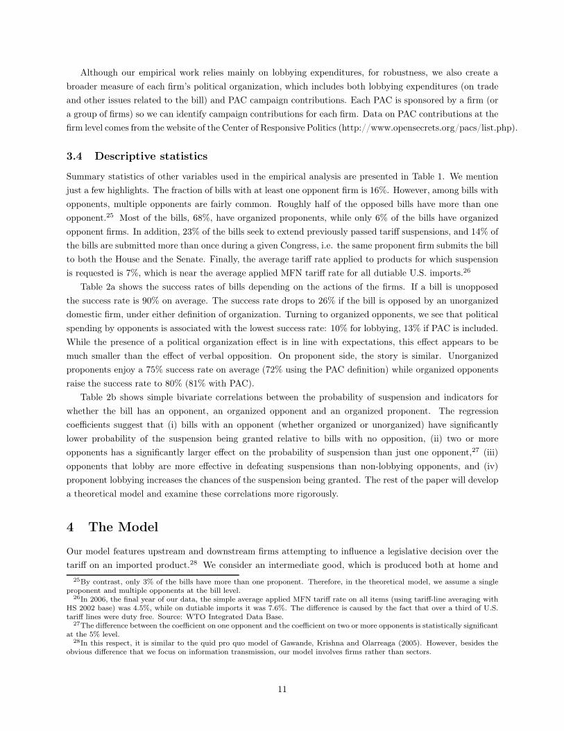
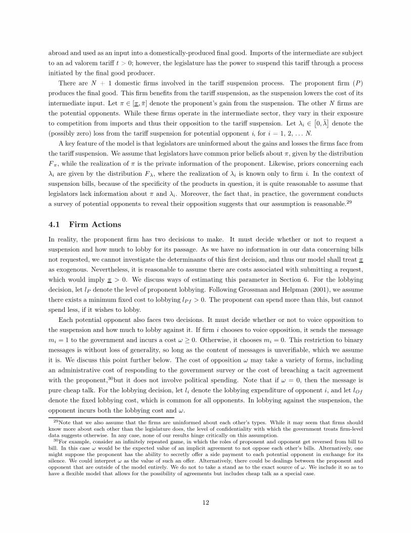
Equations (12) and (13) are illustrated in Figures 3 and 4, which show the lobbying functions and
corresponding suspension probabilities as functions of the firms’ payoffs. In Figure 3, we show (in grey)
proponent lobbying, which equals zero for π < πL, jumps to lPf at π = πL, and increases quadratically
thereafter. The black line shows the probability of suspension, which jumps at π = πL as the legislature
revises upwards its expectation of π based on the jump in lobbying, and increases linearly in π thereafter.
Figure 4 shows similar patterns for each opponent. The difference is that at λi < λO the opponent does not
verbally oppose the suspension, while for λi ≥ λO it does. This causes a downward jump in the probability
of suspension at λi = λO, followed by a second downward jump at λi = λL as the opponent starts to lobby.
5 Empirical Analysis
In this section, we investigate the implications of our model and estimate empirical specifications derived
from the model. The model has three sharp predictions. The first is that, all else equal, effective lobbying
expenditure by the proponent raises the probability of securing a tariff suspension. Second, verbal opposition
itself, without opponent lobbying expenditures, reduces the probability of a suspension; the higher the
number of opponents, the larger is the reduction in the probability of suspension. Third, effective lobbying
expenditures by the opponents decrease the probability of the suspension.
5.1 Empirical strategy
Our estimation is based on equation (13). To begin, we abstract from the lobbying expenditure levels and
consider only the effects of political organization. This simplification allows for comparison with the quid
pro quo literature, which takes this approach. The regression equation is specified as follows:
Pr(suspension)i,t = a + β0Noppi,t + β1N
org,oppi,t + β2D
org,propi,t + β3Zi,t + ηs + νt + εi,t (14)
17

where i and t denote the bill and Congress, respectively, and s denotes the HTS section.35 Pr(suspension)
is the probability that the suspension requested in the bill is granted; Noppi,t is the number firms that voice
opposition; Norg,oppi,t is the number of politically organized opponents, i.e. the number of opponent firms
which lobby on trade or any other issue pertaining to the bill; Dorg,propi,t is a dummy which is equal to 1 if
the proponent firm of the bill is politically organized, i.e. it lobbies on trade or any other issue pertaining to
the bill. Zi,t denotes the vector of additional controls at the bill-congress level. The control variables include
the pre-suspension tariff rate, the (logs of the) number of contacted firms, the number of bills sponsored by
the same member of Congress, and estimated tariff revenue loss; a dummy which is equal to 1 if the bill is an
extension of a previous bill, and a dummy which is equal to 1 if the bill is presented both in the House and
Senate. In addition, we also include political variables: a dummy which is equal to 1 if the sponsor belongs
to the House Ways and Means or Senate Finance Committees in the current or past three Congresses and a
dummy equal to 1 if the sponsor belongs to the Democratic Party. All regressions include HTS section and
Congress fixed effects (denoted, respectively, by ηs and νt). Finally, we also include interactions between
party of the sponsor and Congress fixed effects to control for additional political variables, e.g. whether
the sponsor belongs to the same party as the chairman of Senate Finance and House Ways and Means
committees, whether the sponsor belongs to the majority party in the Congress. Consistent with theoretical
model, equation (14) is estimated using a linear probability model.36
The parameters of interest are β0, β1 and β2. In terms of equation (13), we can interpret these parameters
as β0 = −β (Λ − Ω) /2δ < 0, β1 =−β(λL − Λ)LO/2δ < 0 and β2 = α(πL − Π)LP /2δ > 0, where LO is the
average effective lobbying expenditure of organized opponents. In this specification, we treat the level
of effective lobbying expenditures of opponents and proponent as part of the parameter to be estimated.
Variation in effective lobbying expenditures, both across observations and across individual opponents for
the same observation, is ignored.
In our second specification, we estimate equation (13), explicitly accounting for variation in the levels of
lobbying expenditures of the proponents and opponents. The regression equation is specified as follows:
Pr(suspension)i,t = a + θ0Noppi,t + θ1SLopp
i,t + θ2Lpropi,t + θ3Zi,t + ηs + νt + εi,t (15)
where Lpropi,t denotes the effective lobbying expenditures by the proponent for trade or other issues related to
the bill, and SLoppi,t denotes the sum of effective lobbying expenditures for organized opponents. Recall from
equation (13) that the effective lobbying expenditures depend on (logs of) the minimum feasible lobbying
expenditures lPf and lOf . Note that these values are assumed to be constant across bills and firms of
the same type. Thus, as proxies for lPf and lOf , we choose the minimum lobbying expenditures in the
data, over all firms and bills, for the proponents and opponents, respectively. In this specification, the
coefficients correspond to the theory according to: θ0 = −β (Λ − Ω) /2δ < 0, θ1 =−β(λL − Λ)/2δ < 0 and
θ2 = α(πL − Π)/2δ > 0.
5.2 OLS benchmark results
We first estimate the model using ordinary least squares. Table 3 presents our main results. We find a
strong, negative and significant (at the 1% level) impact of opposition on the probability of passage of the
35There are 22 different HTS sections, which group products into broad categories such as mineral products, chemical orallied industries, textiles, base metals, machinery and mechanical appliances, etc. See: http://hts.usitc.gov/
36Our results are robust to estimation by probit. However, there is a danger with fixed-effects estimation of a probit modelthat it may lead to inconsistent estimates, due to the incidental parameter problem (Chamberlain, 1984).
18

tariff suspension bill. This result is robust across specifications; in particular it is not affected by whether we
measure political organization using a discrete or a continuous variable (compare columns (1)-(2) to columns
(3)-(4)).
Note that the estimate of the coefficient of Noppi,t (i.e., β0) captures the impact of firms that oppose
suspension but do not lobby, since the regression equation controls for Norg,oppi,t . More precisely, all else
equal, each unorganized opponent firm decreases the probability of suspension by −β0. The fact that β0 is
negative and significant is not consistent with the model of Grossman and Helpman (1994). That model
predicts that a product with unorganized domestic producers should actually receive less protection than
products with no domestic producers at all. In fact they should receive a negative tariff, or an import subsidy.
In the case of tariff suspension bills, a zero tariff is the lower bound. So, if we interpret firms that express
opposition without spending to be unorganized producers and those that do not express opposition to be
nonproducers, Grossman and Helpman (1994) would predict that the effect of opposition without spending
increases the likelihood of a suspension being granted. In contrast, according to our estimates in columns (1)
and (2), each unorganized opponent reduces the probability of suspension by 19 percentage points. Therefore,
tariff suspensions do not fit well into a pure quid pro quo model. Rather, they are consistent with our model
of informational lobbying. The coefficient of Noppi,t can be interpreted as a measure of the impact of the
message alone. The fact that it is negative and significant tells us that simply noting opposition does impact
the passage of a bill.
Our results also show that Norg,oppi,t , the political organization of the opponent firm(s), is effective at
reducing the likelihood that the tariff suspension passes. This estimates in columns (1) and (2) are significant
at the 1% level. The coefficient β1 on organized opposition (-24.4 percentage points in column (1)) captures
the additional effect (beyond the impact of unorganized opposition) of opponent lobbying on the probability of
the legislation’s passage. Therefore, a bill with one firm noting opposition, that also lobbies, is 42 percentage
points less likely to pass. The coefficient of Norg,oppi,t can be interpreted as a measure of the impact of lobbying.
The finding that it is negative and statistically significant suggests that lobbying by opponents is effective in
reducing the bill’s passage. The findings are similar if we use effective lobbying expenditures by opponents
instead of the discrete variable (columns (3) and (4)). As predicted by the theoretical model, higher effective
lobbying expenditure by opponents reduces the probability of the suspension being passed. The estimated
effect is statistically significant at the 5 percent level.37 As argued above, it is difficult to disentangle the
motives for lobbying based on political spending. Hence either (both) the information channel, which is the
focus of this paper, or (and) the quid pro quo channel could be driving this result.
On the proponent side, columns (1) and (2) show no significant impact of political organization by the
proponent firm. However, when we use the continuous lobbying variable (which is more consistent with
the estimating equation derived from the theory), we do find that higher proponent lobbying increases the
chances of the suspension being passed (statistically significant at least at the 10% level, columns (3) and
(4)).
Finally, note that the indicator variable of whether the bill is an extension is positive and significant.
Surprisingly, none of the other economic and political controls, except Congress dummies, have a significant
effect on the probability of suspension.
37Note that the effective lobbying expenditures=constant+[Log (lobbying expenditures)]. Therefore, the estimates in column(3) and (4) suggest that a one percent rise in actual lobbying expenditures by opponents reduces the chances of passage of billby about 3.7 percentage points.
19

5.3 IV results
Endogeneity is an issue for both regressions (14) and (15). All three of our main variables, Noppi,t , Norg,opp
i,t ,
Dorg,propi,t in regression (15) and Nopp
i,t , SLoppi,t , Lprop
i,t in regression (15), could be endogenous due to reverse
causality. For example, if the ex-ante expected probability of suspension is high – for some reason we do
not account for in the right-hand-side of the equation – potential opponent firms may decide not to come
forward and oppose the bill, expecting a small impact of their opposition and, at the same time, not wanting
to incur the cost of opposition (for instance, a potential opponent might wish to avoid provoking retaliation
from the proponent, in the event that their roles are reversed on another bill). Similarly, if the probability
of success of a bill is high, opponent firms may decide it is not worthwhile to invest in lobbying expenditures
to try to block it. These reverse-causality effects would imply a negative correlation between the unobserved
component of the probability of suspension and Noppi,t , SLopp
i,t ; hence, they would exaggerate the magnitude
of the (negative) estimated effects.38 Finally, the decision of a proponent firm to invest (and how much) in
lobbying expenditures could also be related to expectations regarding its probability of suspension, and bias
the estimated coefficients on Dorg,propi,t and Lprop
i,t .
To address the endogeneity problems described above, we use an instrumental variables strategy. We use
three different instruments for the number of opponents Noppi,t . First, we construct a variable intended to
capture the possibility that potential opponents are proponents themselves on other bills. Specifically, we
measure the number of potential opponent firms contacted for the bill in question that are also currently
proponents on other bills. The idea underlying the instrument is that these opponents are not likely to voice
opposition if they fear retaliation. Hence, when the value of this instrument is higher, we expect a smaller
number of opponents (first stage). The second instrument is the number of potential opponent firms that
have expressed opposition in past (or current) Congresses. We expect that, the higher is this number, the
higher should be the number of opponents (first stage). In other words, we assume that certain firms have
expertise or are more accustomed to expressing opposition; thus, if a bill has a larger number of potential
opponents that have expressed opposition in the past, it is likely to have a larger number of opponents in the
current period. Finally, the third instrument is the number of potential opponents contacted in the past.39
The higher is this number, the lower the number of actual opponents is likely to be, because after controlling
for the firms that have voiced opposition in the past, this number captures the effect those contacted in the
past that did not oppose.
The three instruments we use for the number of opponents are variables related to the exogenous cost
of opposition and are therefore correlated with the number of opponents, as confirmed in the first stage
regressions (Table 5). In addition, they capture information that is not (readily) available to legislators.
Thus, the three instruments are not likely to affect the probability that legislators grant the tariff suspension
unless they have an impact on the number of opponents. The reason is that the USITC reports include only
the names of contacted firms of the bill in question but do not include details about whether the contacted
firms are themselves proponents on other current bills, whether they have been contacted in the past or
whether they have expressed opposition in past (current) Congresses (the latter three variables being the
38However, the same type of argument may work in the opposite direction, i.e. upstream firms may be more inclined to comeforward and oppose the bill and invest in lobbying expenditures when they fear that the suspension is more likely to be granted.This case is not problematic for us since our estimates of opponent effects would be biased towards zero, i.e. they would be alower bound of the true negative effects.
39Note that the lists of contacted firms are compiled by ITC staff who are not close to the top of the hierarchy, hence are notlikely to be related to decisions made by the Congress regarding the passage of the bills. In discussing how potential opponentsare selected, Pinsky and Tower (1995, p. 20) note, “the ITC generally relies on the expertise of an industry analyst for theseassessments (interview).”
20

instruments we use). There are as many as 69 contacted firms for a single bill and the three variables are
based on details related to both the Current and past Congresses; thus extensive research is required to
acquire this type of information. Most importantly, the fact that Congress does not request this information
from the USITC – given that USITC is the agency with the capacity and institutional responsibility to
gather information needed by policymakers to make the decision on the tariff suspension – indicates it is not
important to the decision. On the other hand, there is evidence that the format of the USITC reports have
changed in the past to accommodate the information needs of the decisionmakers. In particular only starting
with the 106th Congress were the results of the questionnaire sent to contacted firms included in the reports.
To conclude, based on the institutional set-up of the program, we believe that the three instruments for the
number of opponents affect the probability of suspension only indirectly through the endogenous regressor.
To construct instruments for the number of politically organized opponent firms Norg,oppi,t and whether the
proponent firm is politically organized Dorg,propi,t , we use firm-level data on lobbying activity. In particular, for
each firm which spends lobbying money on trade or other issues related to the bill, we consider whether or not
it lobbies for other issues, i.e., issues unrelated to the bill, like, defense.40 We use as instruments the number
of opponents who lobby on unrelated issues and a dummy equal to 1 if the proponent lobbies on unrelated
issues. A firm which lobbies for unrelated issues is likely to have overcome many of the fixed costs associated
with lobbying, and thus it would be easier for the firm to channel lobbying money to influence decisions
regarding the tariff suspension bill. Thus, we expect to find strong first-stage relationships. At the same
time, there is no reason why the lobbying activity of the firm on unrelated issues should have a direct impact
on the probability of passage of the tariff suspension (exclusion restriction). Thus, the number (indicator) of
opponent (proponent) firm lobbying on unrelated issues plausibly allows us to address endogeneity. Finally,
for the measure of effective lobbying expenditures (Lpropi,t , SLopp
i,t ) , we use as instruments the number of
unrelated issues the opponent firms and the proponent firm lobby for, respectively.41
Table 4 presents the results of the IV estimation. Table 5 shows the first-stage estimates, which suggests
that the instruments are very strong. According to regression (1a), Table 5, the number of opponents is
strongly correlated with the three instruments (at the 1% level) with the expected signs. First, the number
of opponents is decreasing in the exposure of opponents to retaliation, increasing in the number of potential
opponents that have expressed opposition in current or past Congresses, and decreasing in the number of
potential opponents contacted in the past. Similarly, column (1b) shows that the number of organized
opponent firms is positively and significantly correlated (at the 1% level) with the number of opponent
firms that lobby on unrelated issues. Regression (1c) shows a similar result for the instrument of political
organization of the proponent firm, which is positively and significantly correlated (at the 1% level) with
whether the proponent firm lobbies on other issues. All these results are unchanged (in terms of sign and
significance level) when we add the control variables in regressions (2a)-(2c). According to regressions (3b)
and (4b), the number of unrelated issues for which the opponent firm lobbies is a positive and significant
determinant (at the 1% level) of (log) lobbying expenditures by the opponent firm on trade and other issues.
A similar relationship holds for the proponent firm (see regressions (3c) and (4c)). To conclude, the first-
stage results are very strong, as also confirmed by the first-stage F statistics for the excluded instruments
reported at the end of Table 4. The high values of the Kleibergen-Paap rk Wald F statistic (between 15.6 and
16.9, 5% Stock-Yogo critical value of 9.53) also suggest that we reject the null of weak correlation between
40To be precise, “issues unrelated to the bill” include all issues in Table B1, except trade, chemicals, mining, food, manufac-turing, textiles and transport.
41Recall that the lobbying reports do not provide the split of total lobbying expenditures among various issues and we derivelobbying expenditures on unrelated issues also from the total expenditures. In order to avoid a mechanical correlation betweenthe instrument and the regressor, we do not use the expenditures on unrelated issues as instrument.
21

the excluded instruments and the endogenous regressors.42
The second-stage results confirm most of the OLS results. The test of overidentifying restrictions passes
by a large margin (the p-value for the Hansen’s J-statistic ranges between 0.92 and 0.97).43 Both unorganized
and organized opposition have a negative and significant impact on the likelihood of passage of the tariff
suspension bill. In addition, proponent firm’s political organization now has a positive and significant impact,
as predicted by the theoretical model. All these findings are confirmed when we use the level of effective
lobbying expenditures to measure the extent of political organization of opponent and proponent firms.
The magnitude of the estimated coefficients on organized proponents is much higher in the IV regressions
compared to the OLS. For example, in regression (1) of Table 4, a bill with an organized proponent is more
than twice as likely to pass (compared to Table 3). The direction of the bias suggests a negative correlation
between the unexplained probability of suspension and proponent lobbying in the OLS regressions. In other
words, bills with a higher ex-ante expected probability of suspension are likely to be associated with a lower
degree of proponent political organization. Finally, note that the pre-suspension tariff rate has a positive
impact on the likelihood of suspension, which suggests that the higher the initial level of distortion and the
loss to the proponents, the less likely the legislature is to yield to pressure from opponents.44
In Table 6, we instrument for the existing tariff rate. One reason to be concerned about the endogeneity
of the existing tariff is that perhaps the parties involved in negotiating the existing MFN tariff during the
Uruguay Round (1986-94) anticipated the likelihood of a tariff suspension in the future, which could create a
reverse causality problem. Another is that omitted variables affecting the existing tariff could also affect the
likelihood of a tariff suspension. We actually regard reverse causality as unlikely because the existing tariff
rate and the tariff suspension are determined at different levels of aggregation: the tariff rate is negotiated
at the “tariff line” (8-digit HS) level, while the tariff suspension affects very specific products that need not
correspond to a single tariff line and typically accounts for only a small fraction of one. Moreover, suspensions
are temporary. Thus, it is unlikely that the possibility of getting a suspension on a very specific product in
a single bill affects the determination of the tariff rate for an entire tariff line. Nevertheless, we might be
concerned that, for example, domestic producers that are “well-connected” enough to obtain high existing
tariff protection might also be more influential in preventing tariff suspensions. This is not a concern when it
comes to foreign determinants of U.S. tariffs, because foreign actors play no rule in the suspensions process.
For this reason, we instrument for the existing tariff rate using international variables shown by Ludema
and Mayda (2009, 2013) to influence MFN tariffs, namely, the share of imports from U.S. FTA partners in
total imports and the Herfindahl index defined over shares of imports from all WTO countries in total MFN
imports, excluding U.S. FTA parters, both at the six-digit HS level. These instruments turn out to be fairly
weak, which argues for the use of limited information maximum likelihood estimation. The results (Table
6) are essentially the same is in Table 4, though effect of the tariff rate itself is now positive but statistically
insignificant.
Besides endogeneity, another possible source of concern is that we observe only suspension bills that
are introduced into Congress. We cannot speak to the determinants of introduction, because it is not
possible to observe bills not introduced. Economic intuition, however, would suggest that proponents refrain
from introducing bills that are doomed to failure, and thus the 79% raw success rate in our sample is not
42Note that both first and second stage IV results are robust to dropping one instrument (for the number of opponents) at atime. The Hansen’s test of overidentifying restrictions is satisfied when we use any two of the three instruments.
43In addition, all the instruments are statistically insignificant when we introduce them in the OLS specification togetherwith the endogenous regressors.
44This is consistent with the finding from trade reforms in many countries, where industries with higher initial tariff rateshad larger reductions in tariffs (see Goldberg and Pavcnik, 2007, for a survey).
22

representative of all conceivable bills. How problematic this is depends in large measure on the scope of
the question being addressed. Both our theory and empirical strategy are designed to capture the effect of
lobbying and verbal opposition on the success rate of bills that have been, and, under the current regime, are
likely to be, introduced into Congress. We believe this to be the most relevant question, and our estimates
are valid in this context.45
To summarize the results, both the OLS and the instrumental variable regressions confirm the key
predictions of the theoretical model: (i) verbal opposition itself, without lobbying, reduces the probability of
suspension, (ii) greater political organization or higher lobbying expenditures by the proponent is associated
with a higher probability of suspension and (iii) greater political organization or higher lobbying expenditures
by the opponent, though relatively rare, is effective at defeating the suspension.
5.4 Robustness checks: Is it really information?
We consistently find that a greater number of opponents reduces the probability of suspension, but how do
we know that this capturing the impact of information conveyed by the contacted firms to legislators? One
of the most obvious concerns is that a simple regression of the probability of suspension on opposition (as in
column (1), Table 2b) is likely to be biased due to the correlation between voicing opposition and spending
by opponent firms. In other words, in those simple regressions, the coefficient on opposition might simply
capture the effect of quid pro quo. By controlling for opponent firms’ lobbying expenditures (on trade and
other issues related to the bill), the theory-based specifications we estimated in Tables 3 and 4 specifically
address this point.
Nevertheless, an additional concern might be that voicing opposition is correlated with other types
of political spending, besides lobbying expenditures. As mentioned in Section 4.1, lobbying expenditures
represent the bulk of total targeted political activity (accounting for up to 90% of it) with the remaining
portion (only approximately 10%) being made up by PAC campaign contributions. In addition, as shown
in Figure 2, at the firm level, lobbying expenditures (on trade and other issues related to the bill) and PAC
contributions are positively and significantly correlated. Thus, we believe that by using lobbying expenditures
data we are accounting for most of the variation in lobbying activity. However, to check the robustness of
our results, we also use firm-level data on PAC campaign contributions, which allows us to fully control for
the impact of lobbying activity. We create a broader measure of political organization where a bill is defined
to have a politically organized opponent (proponent) if the opponent (proponent) makes either lobbying
expenditures on trade or related issues or PAC contributions, or both.46 In addition, in the specifications
in levels, we construct the effective expenditures variables using the sum of lobbying expenditures and PAC
campaign contributions. In other words, the key difference between this table and Tables 3 and 4 is that
the coefficient of the number of opponents represents more strictly the impact of the opponents voicing
opposition without spending on lobbying expenditures or PAC campaign contributions. The estimates are
shown in Table 7. The main result – that verbal opposition reduces the probability of suspension – continues
45If we were interested in the wider population of all potential bills (i.e., those introduced and those not introduced), additionalcomplications could arise. If the proponent’s decision to introduce a bill is a function of exogenous observables, such as the tariffrate or the number of potential opponents, selection does not give rise to a bias in the estimates of the coefficients (Wooldridge,2002). If the introduction of bills is systematically correlated with unobservables that affect the probability of the suspensionbeing granted, then selection bias could occur. As we do not have any information on the bills that are not introduced, itis impossible to implement any of the usual corrections for sample selection. Therefore, we focus our attention only to thesubpopulation of bills that are introduced and will refrain from drawing any conclusions for the wider population.
46According to the broader definition of political organization, 106 and 21 additional bills have politically organized proponentsand opponents, respectively.
23

to hold strongly in most specifications. As in Tables 3 and 4, political organization of opponents (proponents)
reduces (increases) significantly the probability of suspension.
Another concern is that voicing opposition might have a significant effect simply because it may signal to
policymakers that spending by firms in their favor might not take place in the future, if these policymakers
pass the suspension. In that case, the coefficient on voicing opposition would simply capture the impact of
future expected quid pro quo. In general, although firms note opposition without spending money in the
current period, they could be making promises about spending money in future periods; alternatively, they
could have already made the expenditures in previous Congresses. Hence verbal opposition without spending
in the current period may not allow us to accurately measure the impact of information transmission. In
order to address this concern, we define political organization more broadly to include lobbying expenditure
in past, current and future Congresses. The results are reported in Table 8. Again, the number of opponents
controlling for spending money in the past, current or future, significantly reduces the probability of suspen-
sion. Political organization of the opponent is effective in reducing the probability of suspension, whereas
political organization of the proponent increases the probability of suspension.
Yet another concern is that voicing opposition may not actually be conveying any information to legis-
lators that they do not already know. Perhaps legislators are already fully informed about the harm firms
experience from a suspension but merely go through the motions of collecting the information in the interest
of transparency. In this case, the estimated coefficient on the number of opponents could be due to a corre-
lation between voicing opposition and actual harm, where actual harm is what matters to politicians but is
an omitted variable in our regression. This concern is addressed by our instrumental variables strategy. The
instruments we use are variables affecting the incentive for a firm to voice opposition. They are not vari-
ables affecting actual harm. Thus, the significant negative effect of voicing opposition in our IV regressions
suggests that it is voicing opposition rather than actual harm that has influence.
A final concern is that perhaps the only actionable information being conveyed by the number of oppo-
nents is the existence of opposition, not its scale. This might be true if the legislature were operating under
a rule that tariff suspensions must be Pareto improving for firms. However, as explained in the introduction,
we find evidence in the data of numerous violations of the Pareto rule. In particular, 20 percent of bills op-
posed by firms are still successful and 10 percent of unopposed bills are not. More importantly, we find that
the scale of opposition makes a difference, both at the extensive and at the intensive margins. Regression (1)
in Table 9 replicates our main OLS specification (Table 3, column 4) but replaces the number of opponent
firms with two variables: the first is a dummy for bills with exactly one opponent, while the second one is a
dummy for bills with two opponents or more (note that these are the same dummy variables we used in the
correlations of Table 2b). Note the table shows only the estimates of the relevant regressors, suppressing con-
trol variables which are same as in the earlier regression. We find that both dummy variables have a negative
and significant effect on the probability that the tariff suspension is passed and, more importantly, that the
two estimates are significantly different at the 10 percent level. Thus, the scale of opposition at the extensive
margin matters. To investigate scale at the intensive margin, we focus on opponent firm employment. To do
this, we must drop from our sample bills that are opposed by only privately-held firms, since our employment
data comes from Compustat, which contains only publicly-traded firms. Regression (2) replicates our main
OLS specification for this restricted sample and finds the results quite similar to those of the full sample.
Regression (3) replaces the number of opponent firms with the following two variables: a dummy variable
indicating whether there is any opposition at all to the tariff suspension bill and its interaction with the size
of the firms (measured with the number of employees of all firms opposing). We find that size matters, i.e.
24

the interaction variable is negative and significant at the 5% level.
To conclude, our robustness checks provide additional evidence that the relevant channel through which
the number of opponents affects the suspension probability is indeed information transmission. The main
results in the paper continue to hold strongly if we include broader measures of political organization, which
account for (i) PAC contributions and (ii) lobbying expenditures in past and future Congresses. In addition,
scale matters, which is not consistent with the Pareto rule.47,48
5.5 Backing out the structural parameters
Having established that firms influence the tariff suspensions with both money and messages, we now return
to the theoretical model to clarify how exactly this influence works. While the coefficient estimates quantify
the effects of the firms’ actions on the probability of suspension, the model enables us to link these effects
to the costs of opposing and lobbying, the distributions of gains and losses, and the legislative bargaining
cost. Our purpose is to quantify the contribution of each factor and to see if the implied parameters are
reasonable.
We begin by examining the relative magnitudes of the point estimates from our preferred specification
(Table 4, Column 4). Using the definitions θ0 = −β (Λ − Ω) /2δ, θ1 =−β(λL−Λ)/2δ and θ2 = α(πL−Π)/2δ,
we find,Λ − Ω
λL − Λ=
θ0
θ1= 5.68 (16)
β (Λ − Ω)
α(πL − Π)=
−θ0
θ2= 9.39 (17)
According to (16), there is nearly a sixfold difference between the effect of voicing opposition (θ0) and the
effect of opponent lobbying (θ1), which is due to the difference in the information content of these two
actions. That is, the legislature’s belief concerning the expected loss to a contacted firm increases by a factor
of six upon that firm voicing opposition as compared to the increase in belief that occurs when that firm
begins to lobby. From (17), there is a ninefold difference between the effect of voicing opposition and the
effect of proponent lobbying. This ratio depends on both the relative amount of information conveyed and
the legislative bargaining cost β/α (= κ).
In what follows, we attempt to decompose the information component from the bargaining-cost com-
ponent in (17). To do this, we start by making use of equilibrium conditions (9) to solve for the implied
lobbying thresholds. These depend on the minimum lobbying expenditures of proponents and opponents,
which we find in the data to be $10, 000 and $6, 700, respectively. Proponents often propose more the one
bill in a given Congress and thus they spread their lobbying expenditures over multiple bills. Therefore, we
set lPf = $1, 667, reflecting the fact that within each Congress the average proponent proposes about six
bills. As the average opponent opposes only one bill, we set lOf = $6, 700. This implies lobbying thresholds
47We also check the robustness of our results to dropping bills that are extensions to previous bills. The results are unaffected.48Another possible concern is that firms that oppose without spending money might be able to convince policymakers to do
what is best for them because these firms receive the support of a large number of voters (and not because these firms crediblyconvey information about what is good for the policymakers). In other words, policymakers do not want to penalize firms that,for example, employ many workers or are very visible in the local economy. In order to address this concern, we control for thenumber of employees in each opponent firm by merging our dataset with data from Compustat. Since Compustat includes onlypublicly listed firms, our sample size reduces drastically by half. Controlling for the number of employees of the opponent firm,we still find that conveying information without spending money continues to reduce significantly the probability of suspension(in the OLS specifications). In order to avoid losing observations, we also estimate a regression including instead of the numberof employees, a dummy for whether the firm is in Compustat, to denote an indicator variable for large firms. The results arequalitatively similar.
25

of,
πL =lPf
θ2= $72, 500 (18)
λL =lOf
−θ1= $175, 500 (19)
Thus, the gain from a individual bill that is required to induce a proponent to lobby far less than the loss
required to induce an opponent to lobby. This perhaps explains why lobbying by proponents is much more
common in the data than lobbying by opponents. About two thirds of proponents lobby, while only 23% of
opponent firms lobby.
To go further, we need to add assumptions regarding legislators’ priors. Since our equilibrium is fully
revealing for π ≥ πL and λ ≥ λL, we need only specify distributions on the intervals[
π,πL)
,[
0,λO)
, and[
λO,λL)
, and only up to the first moments. To keep matters simple we assume uniform priors over these
intervals.49 Using (9) again we obtain,
λO =
(
1 −θ1
θ0
)
λL = $144, 600 (20)
ω = −θOλO = $31, 200 (21)
Λ =λO + λL
2= $160, 000 (22)
Ω =λO
2= $72, 290 (23)
These calculations allow us to assign dollar values on the legislators’ beliefs concerning opponent loss, condi-
tional on the actions of the contacted firms. The jump in expected opponent loss when opposition is voiced
is about ninety thousand dollars ($160,000 - $72,290), compared to the more modest jump of about fifteen
thousand dollars, ($175,500 - $160,000), when lobbying commences. Furthermore, we see that the cost of
opposition that rationalizes these beliefs is about thirty thousand dollars. This cost is enough to prevent
contacted firms from voicing opposition unless their loss exceeds λO.
To complete the quantification of the model, we need to make an assumption about one last parameter:
π, the minimum proponent gain. Simple tariff theory implies that, if the proponent is the sole consumer of
the product, its gain from a tariff suspension should be at least as large as the total loss to import-competing
firms plus the loss of tariff revenue. Drawing on this intuition, we construct a hypothetical lower bound for
each bill by taking the legislature’s belief about the loss to the average unopposed firm Ω multiplied by the
number of contacted firms plus the estimated tariff revenue loss over the three years of the suspension bill.50
We then take the lowest value of this variable in our sample and arrive at an admittedly rough estimate of
$36,000. Using this estimate, we get,
Π =π + πL
2= $54, 230 (24)
49Note that the legislature’s priors need not match the actual distributions of types. Moreover, even if we were to allowpriors to be updated over time based on past play, Bayes’ rule would at most lead to changes in the probabilities assigned toeach interval, not the relative probabilities assigned to points within a given interval. Thus, a legislature that begins with naivepriors would maintain uniform priors over these intervals without violating Bayes’ rule.
50We use average unopposed firm losses, because we are interested in a lower bound. The average unopposed firm’s loss isless than average potential opponent loss. Nonetheless, our lower bound could still be too high, because tariff revenue plusopponent loss could exceed proponent gain. This could occur, for example, if the proponent is not the sole consumer or if thetariff has terms of trade effects. By inflating our estimate of π, these factors would make it harder to find evidence of costlyside-payments, as the amount of information conveyed by proponent lobbying would be underestimated.
26

Thus the jump in the legislature’s belief about the proponent’s gain when the proponent begins lobbying,
($72,500 - $54,230), is roughly on par with the jump in expected opponent loss when an opponent begins
lobbying. Since we know from (16) that the information content of verbal opposition is 5.7 times that of
opponent lobbying, this implies that the disproportionate influence verbal opposition over proponent lobbying
is also due mostly to greater information conveyed by verbal opposition. However, part of the difference is
due to bargaining costs. Using (18), (22), (23) and (24) in (17) yields,
κ =β
α=
−θ0
θ2
(
πL − π)
λL= 1.95 (25)
In other words, bargaining costs add about 95 cents to every dollar transferred between legislators. This
figure somewhat sensitive to our choice of π. Increasing or decreasing π by 50 percent from our assumed
value produces a range of κ ∈ [1, 2.9]. Moreover, it becomes larger if we include a quid pro quo motive for
lobbying, as explained in the appendix. Intuitively, quid pro quo would tend to enhance the effectiveness of
proponent lobbying relative to voicing opposition (since voicing opposition alone involves no transfers to the
legislature). Thus, to account for our empirical finding that voicing opposition is nine times more effective
proponent organization, the bargaining cost would have to be larger in the presence of quid pro quo.
The bargaining cost κ is a measure of the difficulty sponsors face in overcoming opposition in the legisla-
ture. While the data allow us quantify it, they do not explain its source. One possibility might be differences
in firm characteristics between proponents and opponents. Previous studies on trade at the firm level find
that, similar to exporting firms, firms that source from abroad tend to be larger, more productive, more
capital intensive (Bernard, Jensen, Redding and Schott, 2007) and more likely to be foreign owned (Girma
and Görg, 2004) than their non-outsourcing counterparts. While the majority of the firms in our dataset
are privately held (and thus do not disclose financial data), among the publically held, proponent sales are
indeed twice as large as opponent sales on average. News media coverage has depicted tariff suspensions
as unwarranted “earmarks” that enable large, multinational firms to offshore U.S. jobs and harm small U.S.
businesses (Stephens, 2006). Congressional defenders of suspensions frequently point out that suspensions
are carefully chosen to avoid harm to domestic firms, suggesting sensitivity to this public perception.
One final puzzling aspect of the model is our finding of a non-negligible cost of opposition ω. While
there may be administrative costs involved in responding to the USITC survey, it seems unlikely that these
costs would approach thirty thousand dollars. One possible resolution to the puzzle is that the proponents
and opponents talk about suspensions and arrive at tacit agreements to not oppose each other’s bills. The
opposition cost would then be the cost of breaching such an agreement. This cost should depend on the
likelihood that a given contacted firm will be proponent in the future as well as the likelihood that the bill
it proposes will fail should the firm breach the agreement. In our data, 6.5% of all contacted firms became
proponents at some point during the sample period, and the average proponent requests about six bills in
any given Congress. We also know that the probability than an opposed suspension is successful is about
70% lower on average than unopposed suspension. If we assume that firms take the pessimistic view that
any bill they propose following breach will surely be opposed, then cost of breach would be about 28% of the
expected value of a proposed bill. Using our estimates above, the expected proponent gain from the average
proposed bill about $106,200, and 28% of this is $29,740. This suggests that tacit agreements provide a
quantitatively plausible explanation for the cost of opposition.
27

6 Conclusions
We have developed a model that incorporates information as a driver of trade policy and empirically tested its
predictions using data on US tariff suspensions and firm-level information on trade lobbying expenditures.
Our results are consistent with theory and are robust to addressing endogeneity concerns using an IV
estimation strategy. We found that verbal opposition itself, controlling for opponent spending, reduces the
probability of a suspension. Given that they do not lobby (or make contributions), unorganized opponents
should not matter to politicians, except through the welfare (profits, employment, etc.) and, ultimately, votes
that they generate. We interpret the voicing of opposition as informing the government of the welfare/votes
that are at risk should the suspension pass. The big drop in success rates associated with unorganized
opposition is suggestive of the influence of this information.
The probability of a suspension also declines with the trade policy lobbying expenditures of organized
opponents and increases with the expenditures of organized proponents. The finding that messages are
influential implies that the government relies on information possessed by firms; if this is so, it follows from
the model that political spending must also convey information. That said, we cannot rule out the possibility
that lobbying expenditures are also a form of quid pro quo, as quid pro quo spending is observationally
equivalent to signaling in our model. Thus, while the exact mixture of signaling and quid pro quo cannot
be distinguished, we do find that information matters and so does spending. Moreover, we have achieved a
substantial improvement in accuracy over previous work in the estimation of the spending effect by clearly
linking targeted lobbying expenditures to discretionary tariff changes and by using firm level data.
References
[1] Austen-Smith, David, 1992. “Strategic Models of Talk in Political Decision Making.” International Po-
litical Science Review, 13(1): 45-58.
[2] Austen-Smith, David and John Wright, 1994. “Counteractive Lobbying.” American Journal of Political
Science, 38(1): 25-44.
[3] Belloc, M., 2007. “Protection for sale in the EU.” Mimeo, Sapienza University of Rome.
[4] Benard, Andrew B., J. Bradford Jensen, Stephen J. Redding and Peter K. Schott, 2007. “Firms in
International Trade,” Journal of Economic Perspectives, 21(3):105-130.
[5] Bombardini, Matilde, 2008. “Firm Heterogeneity and Lobby Participation.” Journal of International
Economics, 75(2): 329-348.
[6] Bombardini, Matilde and Francesco Trebbi, 2009. “Competition and Political Organization: Together
or Alone in Lobbying for Trade Policy” NBER working paper No. 14771.
[7] Bowen, T. Renee, 2012. “Legislated Protection and the WTO,” Stanford Graduate School of Business,
Research Paper No. 2116.
[8] Bown, Chad P., 2007, “Global Antidumping Database Version 3.0” mimeo, Brandeis University.
[9] Bradford, Scott, 1991. “Protection and jobs: explaining the structure of trade barriers across industries.”
Journal of International Economics, 61(1): 19-39.
28

[10] Chamberlain, G., 1984. Panel data. In: Griliches, Z., Intriligator, M.D. (Eds.), Handbook of Economet-
rics, Vol. 2. North-Holland, Amsterdam.
[11] Chen, Hui, Parsley, David C. and Yang, Ya-wen, 2010. “Corporate Lobbying and Financial Performance.”
Available at SSRN: http://ssrn.com/abstract=1014264
[12] Costinot, Arnaud, 2009. “Jobs, Jobs, Jobs: A ’New’ Perspective on Protectionism.” Journal of the
European Economic Association, 7(5): 1-31.
[13] de Figueiredo, John M. and Cameron, Charles M., 2009. “Endogenous Cost Lobbying: Theory and
Evidence.” CELS 2009 4th Annual Conference on Empirical Legal Studies Paper. Available at SSRN:
http://ssrn.com/abstract=1443559.
[14] de Figueiredo, J. M. and B. S. Silverman 2006. “The returns to lobbying: University lobbying efforts
and the allocation of earmarked academic grants.” Journal of Law and Economics, 49: 597-626.
[15] Dutt, Pushan and Devashish Mitra, 2002. “Endogenous trade policy through majority voting: an em-
pirical investigation,” Journal of International Economics, 58(1),:107-133.
[16] Ederington, Josh and Jenny Minier, 2008, “Reconsidering the Empirical Evidence on the Grossman-
Helpman Model of Endogenous Protection.” Canadian Journal of Economics, 41(3): 501-516.
[17] Eicher, Theo and Thomas Osang, 2002. “Protection for Sale: An Empirical Investigation: A Comment.”
American Economic Review, 92(5): 1702-11.
[18] European Union, 1998, “Commission communication concerning autonomous tariff suspensions and
quotas,” Official Journal of the European Communities (98/C 128/02).
[19] Facchini, Giovanni, Anna Maria Mayda and Prachi Mishra, 2008. “Do Interest Groups Affect US Immi-
gration Policy?” Centre for Economic Policy Research. Discussion Paper.
[20] Fudenberg, Drew and Jean Tirole, 1991. Game Theory. Boston: MIT Press.
[21] Gawande, Kishore and Usree Bandyopadhyay, 2000. “Is Protection for Sale? Evidence on the Grossman-
Helpman Theory of Endogenous Protection.” Review of Economics and Statistics, 82(1): 139-152.
[22] Gawande, Kishore, Pravin Krishna, Marcelo Olarreaga, 2005. “Lobbying Competition Over Trade Pol-
icy” NBER Working Paper No. 11371
[23] Gawande, Kishore, Pravin Krishna and Michael J Robbins, 2006. “Foreign Lobbies and U.S. Trade
Policy.” Review of Economics and Statistics, 88(3): 563-571.
[24] Gawande, Kishore, William Maloney, and Gabriel Montes-Rojas, 2009. “Foreign informational lobbying
can enhance tourism: Evidence from the Caribbean.” Journal of Development Economics, 90(2): 267-
275.
[25] Girma, S. and H. Görg (2004), “Outsourcing, Foreign Ownership and Productivity: Evidence from UK
Establishment-level Data,” Review of International Economics, 12, 5, 817?32.
[26] Goldberg, Pinelopi Koujianou and Giovanni Maggi, 1999. “Protection for Sale: An Empirical Investiga-
tion.” American Economic Review, 89(5): 1135-1155.
29

[27] Goldberg, Pinelopi Koujianou and Nina Pavcnik, 2007. “Distributional Effects of Globalization in De-
veloping Countries.” Journal of Economic Literature, 45(1): 39-82.
[28] Grossman, Gene M. and Elhanan Helpman, 1994. “Protection for Sale.” American Economic Review,
84(4): 833-850.
[29] Grossman, Gene M. and Elhanan Helpman, 2001. Special Interest Politics, Boston: MIT Press.
[30] Grossman, Gene M. and Elhanan Helpman, 2005. “A Protectionist Bias in Majoritarian Politics.” Quar-
terly Journal of Economics, 120(4): 1239-1282
[31] Gokcekus, Omer and Amber Barth, 2007, “Political economy of the U.S. temporary duty suspension
program: An empirical note.” Public Choice, 131:345-350.
[32] Igan, Deniz, Prachi Mishra and Thierry Tressel, “A Fist Full of Dollars: Lobbying and the Financial
Crisis,” NBER Macroeconomics Annual, forthcoming.
[33] Imai, Susumu, Hijime Katayama and Kala Krishnam, 2013, “A Quantile-Based Test of Protection for
Sale,” Journal of International Economics 91 (1), September 2013, 40–52.
[34] Lohmann, Susanne, 1995. “Information, Access and Contributions: A Signaling Model of Lobby-
ing.”Public Choice, 85: 267-284.
[35] Ludema, Rodney D. and Anna Maria Mayda, 2009. “Do Countries Free Ride on MFN?” Journal of
International Economics, 77(2):137-150.
[36] Ludema, Rodney D. and Anna Maria Mayda, 2013. “Do Terms of Trade Effects Matter for Trade
Agreements? Theory and Evidence from WTO Countries.” Quarterly Journal of Economics 128 (4),
1837-1893.
[37] Mayer, Wolfgang, 1984. “Endogenous Tariff Formation.” American Economic Review, 74(5): 970-985.
[38] McCalman, P., 2004. “Protection for sale and trade liberalization: an empirical investigation.” Review
of International Economics, 12: 81-94.
[39] Mitra, D., Thomakos, D., & Ulubasoglu, M., 2002. “Protection for sale in a developing country: democ-
racy versus dictatorship.” Review of Economics and Statistics, 84: 497-508.
[40] Milyo, Jeffrey, David Primo and Timothy Groseclose, 2000. “Corporate PAC Campaign Contributions
in Perspective.” Business and Politics, 2(1): 75-88.
[41] Potters, J. and F. van Winden, 1992. “Lobbying and asymmetric information.” Public Choice, 74: 269-
292.
[42] Pinsky, L., & Tower, E., 1995. “Temporary duty suspension in the United States.” North American
Journal of Economics and Finance, 6(1): 17-36.
[43] Snyder, J. M. 1990. “Campaign contributions as investments: The US House of Representatives 1908-
1986.” Journal of Political Economy, 61: 195-206.
[44] Stephens, J., 2006, “A Quiet Break for Corporations,” The Washington Post, September, 20, 2006.
30

[45] Trefler, D., 1993. “Trade liberalization and the theory of endogenous protection: an econometric study
of U.S. import policy.” Journal of Political Economy, 101: 138-160.
[46] Tripathi, M., S. Ansolabehere, and J. Snyder 2002. “Are PAC contributions and lobbying linked? New
evidence from the 1995 Lobby Disclosure Act.” Business and Politics, 4: 131-155.
[47] Wooldridge, J. M. 2002. Econometric analysis of cross section and panel data, The MIT Press, Cam-
bridge, Massachusetts.
[48] Wright, John R., 1996. Interest Groups and Congress: Lobbying, Contributions, and Influence. Allyn &
Bacon, Boston.
Appendix: The Lobbying Model with Contributions
Our model in the main text treated lobbying expenditures as pure signals of information, whereas Gross-
man and Helpman (1994) assume political spending, in the form of contributions, enters directly into the
politician’s objective function and can be made contingent on the policy choice. Here we adapt our model to
incorporate this assumption. Suppose that at the information stage of the model, each firm decides whether
or not to hire a lobbyist, and, if so, pays the lobbyist a (variable) fee: lP in the case of the proponent, and li in
the case of each opponent. The lobbyist in turn offers a contributions to legislators equal to a fraction ψ of the
fee received from the firm, which is contingent upon passage of the firm’s desired policy. Assume that lobbyist
transfers to opponent legislators bear the same transaction cost κ > 1 as do side-payments from the sponsor.
Thus, without loss of generality we can assume that all lobbyist transfers go to the sponsor. If the suspension
passes, therefore, the sponsor receives ψlP from the proponent lobbyist, while if it fails, it receives ψli from
the opponent lobbyists. Equations (1) and (2) become GP = γP + απ − κ∑N
i=1 si + ψlP − ψ∑N
i=1 li − εP
and Gi = γi + αλi + si − εi.
We assume that any unspent fees are profit for the lobbyists. This ensures that the legislator’s receipt
of contributions is contingent on the policy choice, but the fees paid by the firms are not. The former
assumption is the key component of the quid pro quo model, while the latter is made solely for tractability.51
Given these objective functions, the probability of suspension becomes,
Pr[suspension] =1
2+
γ + απ − βN
∑
i=1
λi + ψ(
lP −∑N
i=1 li)
2δ(26)
The proponent’s expected gain from the suspension net of lobbying expenses becomes,
uP (π, π, lP ) =π
2δ
[
δ + γ + απ + ψlP − NE(βλ + ψli(λ))]
− lP (27)
while potential opponent i’s expected gain net of lobbying expenses is
ui(λ, λi,ωmi + li) = −λ
2δ
[
δ + γ − βλi − ψli + αE(π + lP (π)) − (N − 1)E(βλ + ψli(λ))]
− ωmi − li (28)
51Otherwise, the lobbying cost to the firm depends on the probability of suspension. This makes the mathematics much morecomplicated. The equilibrium lobbying functions can only be determined by solving a system of nonlinear differential equations.Numerical simulations show qualitatively similar results to what is shown here.
31

Because political spending has a direct effect on the probability of spension, it effectively reduces the
marginal cost to a firm of using spending as a signal. To capture this effect, we define the function s(x) =
1−(xψ/2δ), which is the marginal cost of political spending for a firm of type x, holding beliefs constant. We
restrict parameters such that s(x) ∈ [0, 1] for all firm types. Using s(x) in (26) and (27), it straightforward
to solve for the equilibrium threshold values,
α
2δ
(
πL − Π)
πL = s(πL)lPf ,β
2δ
(
λL − Λ)
λL = s(λL)lOf ,β
2δ(Λ − Ω)λO = ω (29)
Comparing (28) to (7), we see that the threshold condition for λO is unchanged. This is because it involves
no spending and thus is unaffected by the introduction of quid pro quo. The spending thresholds are affected
however. The introduction of quid pro quo is equivalent to reducing the fixed costs of lobbying.
The first order conditions for the lobbying expenditures are now given by,
απ
2δ= s(π)
drP
dπ,
βλi
2δ= s(λi)
dri
dλi(30)
These conditions result in more complicated lobbying functions than the quadratic ones in the main text.
However, their log-linear approximation is largely unaffected, resuting in a final estimating equation of,
Pr(suspension) ≈ Γ −β (Λ − Ω)
2δ
N∑
i=1
I[λi>λO ] −β
(
λL − Λ)
2δs(λL)
N∑
i=1
Li +α
(
πL − Π)
2δs(πL)LP (31)
From an empirical standpoint, therefore, the only effect of introducing quid pro quo is on the interpretation
of the coefficients on effective lobbying. In particular, these coefficients now capture the combined effects of
information, quid pro quo, and government preference on the probability of suspension. Note, however, that
this reinterpretation does not help to resolve the puzzle as to why voicing opposition is seven times more
influential proponent organization. In fact, it makes the finding even more striking. To see this, note that
with quid pro quo (17) becomes:β (Λ − Ω)
α(πL − Π)s(πL) =
−θ0
θ2= 9.4 (32)
Since s(πL) < 1, this means that the combined effect of bargaining cost β/α and the information differential
(Λ − Ω) /(πL − Π) must be even greater to account for the ninefold difference in effectiveness. Intuitively,
the presence of quid pro quo should enhance the effectiveness of lobbying relative to voicing oppostion. The
finding voicing opposition is more effective thus cannot be explained by quid pro quo.
32

Figure 2. Scatter Plots between Lobbying Expenditures and Campaign Contributions from Political Action Committees (PACs) at the Firm Level
Campaign contributions from PACs and lobbying expenditures on trade and other issues related to tariff suspension bills
(in millions of US$)
Notes. The scatter plots are based on data on campaign contributions and lobbying expenditures over four election cycles -- 1999-2000, 2001-02, 2003-04 and 2005-06. The correlation between (log) contributions from PACs and (log) lobbying expenditures for trade is 0.504 (robust standard error=0.041; p-value=0.000). Logarithms of zero values of PAC and lobbying expenditures are assumed equal to zero.
05
1015
20
PAC
contr
ibutio
ns b
y firm
s (in
logs
)
0 5 10 15 20Lobbying expend itures on trade and related issues by firms (in logs)
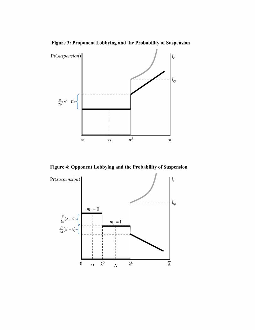
!
€
β2δ
Λ −Ω( ) !
€
Λ
€
λL
€
λ !
€
lOf !€
Pr(suspension) !
€
li !
€
mi = 0 !
Figure 4: Opponent Lobbying and the Probability of Suspension
€
β2δ
λL − Λ( ) !
€
mi =1!
€
Ω
€
λO
€
Π
€
π L
€
π !
€
lPf !
€
α2δ
π L −Π( ) !
Figure 3: Proponent Lobbying and the Probability of Suspension
€
Pr(suspension) !
€
lP !
€
π !
0!
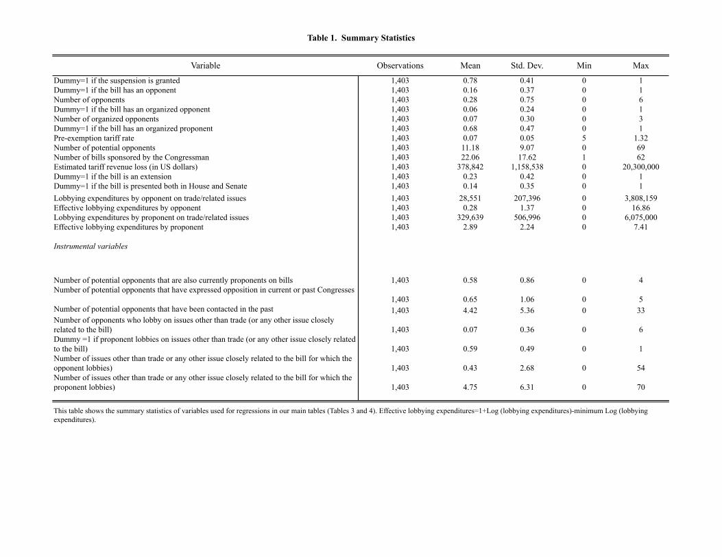
Variable Observations Mean Std. Dev. Min Max
Dummy=1 if the suspension is granted 1,403 0.78 0.41 0 1Dummy=1 if the bill has an opponent 1,403 0.16 0.37 0 1Number of opponents 1,403 0.28 0.75 0 6Dummy=1 if the bill has an organized opponent 1,403 0.06 0.24 0 1Number of organized opponents 1,403 0.07 0.30 0 3Dummy=1 if the bill has an organized proponent 1,403 0.68 0.47 0 1Pre-exemption tariff rate 1,403 0.07 0.05 5 1.32Number of potential opponents 1,403 11.18 9.07 0 69Number of bills sponsored by the Congressman 1,403 22.06 17.62 1 62Estimated tariff revenue loss (in US dollars) 1,403 378,842 1,158,538 0 20,300,000Dummy=1 if the bill is an extension 1,403 0.23 0.42 0 1Dummy=1 if the bill is presented both in House and Senate 1,403 0.14 0.35 0 1Lobbying expenditures by opponent on trade/related issues 1,403 28,551 207,396 0 3,808,159Effective lobbying expenditures by opponent 1,403 0.28 1.37 0 16.86Lobbying expenditures by proponent on trade/related issues 1,403 329,639 506,996 0 6,075,000Effective lobbying expenditures by proponent 1,403 2.89 2.24 0 7.41
Instrumental variables
Number of potential opponents that are also currently proponents on bills 1,403 0.58 0.86 0 4Number of potential opponents that have expressed opposition in current or past Congresses
1,403 0.65 1.06 0 5Number of potential opponents that have been contacted in the past 1,403 4.42 5.36 0 33Number of opponents who lobby on issues other than trade (or any other issue closely related to the bill) 1,403 0.07 0.36 0 6Dummy =1 if proponent lobbies on issues other than trade (or any other issue closely related to the bill) 1,403 0.59 0.49 0 1Number of issues other than trade or any other issue closely related to the bill for which the opponent lobbies) 1,403 0.43 2.68 0 54Number of issues other than trade or any other issue closely related to the bill for which the proponent lobbies) 1,403 4.75 6.31 0 70
Table 1. Summary Statistics
This table shows the summary statistics of variables used for regressions in our main tables (Tables 3 and 4). Effective lobbying expenditures=1+Log (lobbying expenditures)-minimum Log (lobbying expenditures).

Number of Bills Success Rate
Total number of bills 1,403 78%
Bills with Opponents 231 20%Organized 83 10%Unorganized 148 26%
Organized (including PAC) 101 13%Unorganized (including PAC) 130 26%
Bills without Opponents 1,172 90%
Total number of bills 1,403 78%
Organized 949 80%Unorganized 454 75%
Organized (including PAC) 1,055 81%Unorganized (including PAC) 358 72%
Table 2a. Success Rates of Suspension Bills
Notes. Success rate of a bill in each cell is measured by the number of bills passed as a proportion of the total number of bills in that cell. Organized refers to bills with a proponent or opponent firm that makes positive lobbying expenditures on trade or related issues. Organized (including PAC) refers to bills with a proponent or opponent firm that makes positive lobbying expenditures on trade or related issues or makes PAC contributions.
Opponents
Proponents

[1] [2] [3] [4]
Dummy=1 if the bill has an opponent -0.695***[0.028]
Dummy=1 if the bill has only one opponent -0.639***[0.040]
Dummy=1 if the bill has two or more opponents -0.764***[0.035]
Dummy=1 if the bill has an organized opponent -0.731***[0.034]
Dummy=1 if the bill has an organized proponent 0.052**[0.024]
Number of observations 1,403 1,403 1,403 1,403R-squared 0.39 0.40 0.18 0.00
Table 2b. Determinants of Suspensions -- Simple Correlations
Standard errors denoted in parentheses are robust to heteroskedasticity. ***, ** and * represent statistical significance at 1, 5 and 10 percent respectively.
Dependent variable: Dummy=1 if the suspension is granted

[1] [2] [3] [4]
Number of opponents -0.244*** -0.244*** -0.254*** -0.254***[0.027] [0.027] [0.025] [0.026]
Number of organized opponents -0.186*** -0.188***[0.071] [0.073]
Dummy=1 if the bill has an organized proponent 0.027 0.012[0.020] [0.021]
Effective lobbying expenditures by opponent -0.036** -0.036**[0.015] [0.016]
Effective lobbying expenditures by proponent 0.011** 0.009*[0.004] [0.004]
Number of contacted firms (in logs) 0.021 0.025 0.023 0.026[0.018] [0.018] [0.018] [0.018]
Pre-exemption tariff rate 0.16 0.182 0.161 0.183[0.134] [0.140] [0.130] [0.136]
Number of bills sponsored by the Congressman (in logs) -0.005 -0.005 -0.005 -0.005[0.010] [0.010] [0.010] [0.010]
Estimated tariff revenue loss (in logs) 0.001 0.000[0.005] [0.005]
Dummy=1 if the bill is an extension 0.075*** 0.073***[0.018] [0.019]
Dummy=1 if the bill is presented both in House and Senate 0.04 0.038[0.028] [0.028]
Dummy=1 if sponsor belongs to the House Ways and Means or Senate Finance Committees in the current or past three Congresses 0.024 0.015
[0.024] [0.024]
Dummy=1 if sponsor belongs to the Democratic Party 0.016 0.023[0.059] [0.060]
Dummy=1 if bill was proposed by a leader of majority party 0.303 0.31 0.306 0.319[0.269] [0.268] [0.283] [0.283]
Dummy=1 if Congress=107 0.146*** 0.149*** 0.151*** 0.155***[0.039] [0.040] [0.039] [0.040]
Dummy=1 if Congress=108 -0.02 0.031 -0.009 0.038[0.057] [0.068] [0.057] [0.068]
Dummy=1 if Congress=109 0.099*** 0.097*** 0.101*** 0.098***[0.028] [0.033] [0.028] [0.033]
Number of observations 1,403 1,403 1,403 1,403R-squared 0.35 0.36 0.36 0.36
Table 3. Determinants of Suspensions -- Ordinary Least Squares
Standard errors denoted in parentheses are robust to heteroskedasticity. ***, ** and * represent statistical significance at 1, 5 and 10 percent respectively. Effective lobbying expenditures=1+Log (lobbying expenditures)-minimum Log (lobbying expenditures). All regressions include industry and Congress fixed effects. Columns [2] and [4] also include the interactions between Congress fixed effects and party of the sponsor.
Dependent variable: Dummy=1 if the suspension is granted

[1] [2] [3] [4]
Number of opponents -0.219*** -0.226*** -0.211*** -0.216***[0.056] [0.057] [0.049] [0.049]
Number of organized opponents -0.179* -0.168*[0.102] [0.100]
Dummy=1 if the bill has an organized proponent 0.077*** 0.070**[0.028] [0.030]
Effective lobbying expenditures by opponent -0.040** -0.038**[0.018] [0.018]
Effective lobbying expenditures by proponent 0.024*** 0.023***[0.006] [0.006]
Number of contacted firms (in logs) 0.016 0.021 0.014 0.018[0.020] [0.020] [0.020] [0.019]
Pre-exemption tariff rate 0.187 0.197 0.206 0.211[0.140] [0.140] [0.135] [0.136]
Number of bills sponsored by the Congressman (in logs) -0.007 -0.006 -0.007 -0.007[0.010] [0.010] [0.010] [0.010]
Estimated tariff revenue loss (in logs) -0.001 -0.003[0.005] [0.005]
Dummy=1 if the bill is an extension 0.073*** 0.071***[0.019] [0.019]
Dummy=1 if the bill is presented both in House and Senate 0.032 0.034[0.029] [0.029]
Dummy=1 if sponsor belongs to the House Ways and Means or Senate Finance Committees in the current or past three Congresses 0.014 0.003
[0.024] [0.024]
Dummy=1 if sponsor belongs to the Democratic Party 0.023 0.037[0.060] [0.061]
Dummy=1 if bill was proposed by a leader of majority party 0.255 0.271 0.246 0.271[0.264] [0.267] [0.264] [0.265]
Dummy=1 if Congress=107 0.158*** 0.163*** 0.168*** 0.179***[0.040] [0.041] [0.040] [0.041]
Dummy=1 if Congress=108 -0.017 0.019 0.009 0.044[0.056] [0.066] [0.056] [0.066]
Dummy=1 if Congress=109 0.109*** 0.101*** 0.117*** 0.108***[0.030] [0.035] [0.030] [0.034]
Number of observations 1,403 1,403 1,403 1,403R-squared 0.27 0.28 0.27 0.28
Instrumental variables
First-stage F (number of opponents) 25.34 25.27 42.24 41.4First-stage F (number of organized opponents) 17.58 17.78First-stage F (D=1 if bill has an organized proponent) 255.60 245.58First-stage F (effective lobbying expenditures by opponent) 40.84 39.93First-stage F (effective lobbying expenditures by proponent) 71.33 71.32Hansen's J statistic (p value) 0.97 0.95 0.97 0.92
Standard errors denoted in parentheses are robust to heteroskedasticity. ***, ** and * represent statistical significance at 1, 5 and 10 percent respectively. The first-stage regressions are shown in Table 5. The number of opponents; number of organized opponents; dummy for organized proponent; and the effective lobbying expendituresof opponents and proponents, are treated as endogenous. Effective lobbying expenditures=1+Log (lobbying expenditures)-minimum Log (lobbying expenditures). All regressions include industry and Congress fixed effects. Columns [2] and [4] also include the interactions between the Congress fixed effects and party of the sponsor.
Number of opponents who lobby on issues other than trade (or any other issue closely related to the bill)
Number of issues other than trade or any other issue closely related to the bill for which the opponent lobbies
Number of potential opponents that have expressed opposition in current or past Congresses
Number of issues other than trade or any other issue closely related to the bill for which the proponent lobbies
Dummy =1 if proponent lobbies on issues other than trade (or any other issue closely related to the bill)
Number of potential opponents that have expressed opposition in current or past Congresses
Table 4. Determinants of Suspensions --Instrumental Variables Regressions
Dependent variable: Dummy=1 if the suspension is granted
Number of potential opponents that have been contacted in the past
Number of potential opponents that have been contacted in the past
Number of potential opponents that are also currently proponents
Number of potential opponents that are also currently proponents

[1a] [1b] [1c] [2a] [2b] [2c] [3a] [3b] [3c] [4a] [4b] [4c]
Dependent variable: Number of opponents
Number of organized opponents
Dummy=1 if the bill has an
organized proponent
Number of opponents
Number of organized opponents
Dummy=1 if the bill has an
organized proponent
Number of opponents
Effective lobbying
expenditures by opponent
Effective lobbying
expenditures by proponent
Number of opponents
Effective lobbying
expenditures by opponent
Effective lobbying
expenditures by proponent
Number of contacted firms that are also currently proponents -0.221*** 0.009 -0.007 -0.223*** 0.007 -0.008 -0.235*** 0.017 0.198** -0.239*** 0.006 0.163*[0.033] [0.008] [0.017] [0.032] [0.008] [0.017] [0.035] [0.037] [0.093] [0.034] [0.037] [0.091]
Number of potential opponents that have been contacted in the past -0.030*** -0.002 0.003 -0.029*** -0.001 0.004 -0.029*** 0 0.046*** -0.028*** 0.003 0.053***[0.005] [0.002] [0.003] [0.005] [0.002] [0.003] [0.005] [0.006] [0.015] [0.005] [0.007] [0.016]
Number of contacted firms that have expressed opposition in current or past Congresses 0.211*** 0.009 -0.012 0.204*** 0.009 -0.018 0.233*** 0.060* -0.384*** 0.231*** 0.060* -0.397***[0.028] [0.008] [0.013] [0.028] [0.008] [0.013] [0.028] [0.034] [0.061] [0.028] [0.034] [0.059]
Number of opponents which lobby on other issues 0.849*** 0.669*** -0.016 0.834*** 0.668*** -0.019[0.172] [0.109] [0.037] [0.171] [0.110] [0.037]
Dummy=1 if the bill has a proponent which lobbies on other issues 0.007 0.035*** 0.707*** -0.017 0.032*** 0.697***[0.030] [0.009] [0.020] [0.032] [0.010] [0.021]
Number of other issues for which the opponent lobbies 0.118*** 0.513*** -0.120*** 0.116*** 0.511*** -0.121***[0.011] [0.047] [0.026] [0.011] [0.047] [0.027]
Number of other issues for which the proponent lobbies 0.013*** 0.013** 0.247*** 0.012** 0.012** 0.240***[0.005] [0.006] [0.017] [0.005] [0.006] [0.017]
Number of contacted firms (in logs) 0.372*** 0.009 0.028* 0.377*** 0.009 0.037** 0.357*** -0.065 -0.167* 0.362*** -0.062 -0.112[0.048] [0.010] [0.016] [0.047] [0.010] [0.017] [0.047] [0.042] [0.093] [0.047] [0.043] [0.095]
Pre-exemption tariff rate -0.395 0.312 -1.088*** -0.304 0.316 -1.008*** -0.367 1.909* -0.534 -0.312 1.963* 0.014[0.272] [0.201] [0.157] [0.284] [0.207] [0.158] [0.285] [1.117] [0.595] [0.300] [1.150] [0.713]
Number of bills sponsored by the Congressman (in logs) 0.007 0.008* 0.020** 0.007 0.010** 0.011 0.001 0.014 0.094** -0.001 0.017 0.064[0.016] [0.005] [0.009] [0.017] [0.005] [0.010] [0.016] [0.020] [0.048] [0.016] [0.021] [0.051]
Estimated tariff revenue loss (in logs) 0.015* -0.002 -0.006 0.015 0.01 0.063**[0.009] [0.002] [0.005] [0.009] [0.011] [0.025]
Dummy=1 if the bill is an extension -0.053* -0.011 0.067*** -0.053* -0.019 0.283***[0.028] [0.008] [0.022] [0.028] [0.034] [0.100]
Dummy=1 if the bill is presented both in House and Senate -0.045 0.026* 0.090*** -0.027 0.158** 0.172[0.039] [0.014] [0.027] [0.040] [0.066] [0.130]
Dummy=1 if sponsor belongs to the House Ways and Means or Senate Finance Committees in the current or past three Congresses 0.045 0.028* 0 0.02 0.072 0.168
[0.041] [0.014] [0.020] [0.043] [0.046] [0.111]Dummy=1 if sponsor belongs to the Democratic Party 0.002 0.038 -0.048 -0.013 0.06 -0.448*
[0.078] [0.024] [0.050] [0.062] [0.121] [0.249]Dummy=1 if bill was proposed by a leader of majority party 1.087 0.334* -0.013 1.013 0.316 -0.017 1.091 1.604* 1.526*** 1.031 1.533* 1.230**
[0.754] [0.200] [0.054] [0.762] [0.202] [0.061] [0.754] [0.928] [0.589] [0.764] [0.926] [0.570]Dummy=1 if Congress=107 -0.006 0.006 -0.127*** -0.044 0.016 -0.139*** -0.063 -0.121* -1.563*** -0.092 -0.096 -1.828***
[0.054] [0.014] [0.034] [0.055] [0.017] [0.040] [0.058] [0.070] [0.178] [0.058] [0.070] [0.189]Dummy=1 if Congress=108 -0.128* 0.026 -0.095*** -0.016 0.045 -0.022 -0.113 0.190* -0.762*** -0.049 0.21 -0.871***
[0.076] [0.022] [0.034] [0.110] [0.032] [0.029] [0.076] [0.098] [0.210] [0.108] [0.128] [0.268]Dummy=1 if Congress=109 -0.046 0.008 -0.04 -0.005 0.022 -0.017 -0.026 0.026 -0.086 0.01 0.098 0.035
[0.053] [0.018] [0.029] [0.062] [0.022] [0.033] [0.049] [0.060] [0.141] [0.056] [0.068] [0.157]
Number of observations 1,403 1,403 1,403 1,403 1,403 1,403 1,403 1,403 1,403 1,403 1,403 1,403R-squared 0.48 0.69 0.56 0.49 0.70 0.58 0.46 0.75 0.52 0.47 0.75 0.55
Table 5. Determinants of Suspensions --First Stage Instrumental Variables Regressions
Standard errors denoted in parentheses are robust to heteroskedasticity. ***, ** and * represent statistical significance at 1, 5 and 10 percent respectively. All regressions include industry and Congress fixed effects. Columns [2a]-[2c] and [4a]-[4c] also include interactions between the Congress fixed effects and party of the sponsor.

[1] [2] [3] [4]
Number of opponents -0.216*** -0.223*** -0.218*** -0.220***[0.058] [0.060] [0.051] [0.052]
Number of organized opponents -0.190* -0.176[0.109] [0.108]
Dummy=1 if the bill has an organized proponent 0.113** 0.102**[0.045] [0.047]
Effective lobbying expenditures by opponent -0.042** -0.041**[0.020] [0.020]
Effective lobbying expenditures by proponent 0.024*** 0.024***[0.007] [0.007]
Number of contacted firms (in logs) 0.03 0.029 0.033 0.032[0.027] [0.024] [0.027] [0.025]
Pre-exemption tariff rate -1.841 -1.25 -2.179 -1.713[2.032] [1.841] [2.187] [2.096]
Number of bills sponsored by the Congressman (in logs) -0.007 -0.007 -0.007 -0.006[0.011] [0.011] [0.011] [0.012]
Estimated tariff revenue loss (in logs) 0.001 0.000[0.006] [0.006]
Dummy=1 if the bill is an extension 0.065*** 0.066***[0.021] [0.021]
Dummy=1 if the bill is presented both in House and Senate 0.029 0.035[0.030] [0.031]
Dummy=1 if sponsor belongs to the House Ways and Means or Senate Finance Committees in the current or past three Congresses -0.009 -0.013
[0.027] [0.028]
Dummy=1 if sponsor belongs to the Democratic Party 0.021 0.027[0.065] [0.067]
Dummy=1 if bill was proposed by a leader of majority party 0.236 0.273 0.242 0.282[0.273] [0.273] [0.279] [0.277]
Dummy=1 if Congress=107 0.178*** 0.180*** 0.187*** 0.196***[0.051] [0.051] [0.052] [0.050]
Dummy=1 if Congress=108 -0.051 -0.035 -0.033 -0.013[0.068] [0.080] [0.069] [0.080]
Dummy=1 if Congress=109 0.074 0.07 0.071 0.064[0.047] [0.055] [0.050] [0.060]
Number of observations 1230 1230 1230 1230R-squared 0.20 0.24 0.18 0.22
Instrumental variables
First-stage F (number of opponents) 16.2 16.3 27.2 26.38First-stage F (number of organized opponents) 21.2 20.7First-stage F (D=1 if bill has an organized proponent) 186.4 182.9First-stage F (effective lobbying expenditures by opponent) 26.68 25.53First-stage F (effective lobbying expenditures by proponent) 43.18 44.30
First-stage F (tariff rate) 4.4 4.3 3.4 3.0Hansen's J statistic (p value) 0.8 0.7 0.9 0.7
Herfindahl index defined over shares of imports from WTO members in total imports, excluding FTA partners.
Table 6. Determinants of Suspensions--Instrument for Tariff (Limited Information Maximum Likelihood)
Dependent variable: Dummy=1 if the suspension is granted
Number of potential opponents that are also currently proponents
Number of potential opponents that are also currently proponents
Number of potential opponents that have expressed opposition in current or past Congresses
Number of potential opponents that have expressed opposition in current or past Congresses
Herfindahl index defined over shares of imports from WTO members in total imports, excluding FTA partners.
Standard errors denoted in parentheses are robust to heteroskedasticity. ***, ** and * represent statistical significance at 1, 5 and 10 percent respectively. The first-stage regressions are not shown. The number of opponents; number of organized opponents; dummy for organized proponent; and the effective lobbying expendituresof opponents and proponents, and the tariff rate are treated as endogenous. Effective lobbying expenditures=1+Log (lobbying expenditures)-minimum Log (lobbying expenditures). All regressions include industry and Congress fixed effects. Columns [2] and [4] also include the interactions between the Congress fixed effects and party of the sponsor.
Number of potential opponents that have been contacted in the past
Number of potential opponents that have been contacted in the past
Number of opponents who lobby on issues other than trade (or any other issue closely related to the bill)
Number of issues other than trade or any other issue closely related to the bill for which the opponent lobbies
Dummy =1 if proponent lobbies on issues other than trade (or any other issue closely related to the bill)
Number of issues other than trade or any other issue closely related to the bill for which the proponent lobbies
Share of imports from FTA partners in a total imports. Share of imports from FTA partners in a total imports.

[1] [2] [3] [4] [5] [6] [7] [8]Number of opponents -0.240*** -0.240*** -0.252*** -0.251*** -0.192*** -0.199*** -0.192*** -0.193***
[0.029] [0.030] [0.029] [0.029] [0.067] [0.068] [0.056] [0.056]
Number of organized opponents (makes lobbying expenditures or PAC contributions) -0.142** -0.146** -0.196* -0.185*
[0.058] [0.060] [0.108] [0.107]Dummy=1 if the bill has an organized proponent (makes lobbying expenditures or PAC contributions) 0.024 0.005 0.101*** 0.095**
[0.023] [0.024] [0.037] [0.040]Effective lobbying expenditures and PAC contributions by opponent -0.022** -0.022** -0.033** -0.032**
[0.011] [0.011] [0.015] [0.015]Effective lobbying expenditures and PAC contributions by proponent 0.009** 0.006 0.026*** 0.027***
[0.004] [0.004] [0.007] [0.007]Number of contacted firms (in logs) 0.023 0.028 0.024 0.028 0.014 0.018 0.012 0.014
[0.018] [0.018] [0.018] [0.018] [0.021] [0.021] [0.020] [0.020]Pre-exemption tariff rate 0.193 0.212 0.193 0.215 0.288* 0.288* 0.298** 0.301**
[0.140] [0.149] [0.135] [0.142] [0.162] [0.161] [0.147] [0.145]Number of bills sponsored by the Congressman (in logs) -0.003 -0.003 -0.005 -0.006 -0.005 -0.005 -0.009 -0.008
[0.010] [0.010] [0.010] [0.010] [0.010] [0.010] [0.010] [0.010]Estimated tariff revenue loss (in logs) 0.000 0.000 -0.002 -0.004
[0.005] [0.005] [0.005] [0.005]Additional controls No Yes No Yes No Yes No YesNumber of observations 1,403 1,403 1,400 1,400 1,403 1,403 1,400 1,400R-squared 0.35 0.36 0.35 0.36 0.26 0.27 0.26 0.26First-stage F (opponent) 25.34 25.27 42.35 41.48First-stage F (organized opponent) 20.88 20.38First-stage F (organized proponent) 138.06 136.01First-stage F (opponent lobbying expenditures) 37.95 35.68First-stage F (proponent lobbying expenditures) 64.93 65.17Hansen's J statistic (p value) 0.96 0.93 0.98 0.88
Dependent variable: Dummy=1 if the suspension is granted
OLS IV
Standard errors denoted in parentheses are robust to heteroskedasticity. ***, ** and * represent statistical significance at 1, 5 and 10 percent respectively. Effective lobbying expenditures=1+Log (lobbying expenditures)-minimum Log (lobbying expenditures). The number of opponents; number of organized opponents; dummy for organized proponent; and the effective lobbying expendituresof opponents and proponents, are treated as endogenous. All regressions include industry and Congress fixed effects. Columns [2], [4], [6] and [8] also include interactions between the Congress fixed effects and party of the sponsor. The additional controls are the same as Table 4. All instruments are identical to Table 4.
Table 7. Determinants of Suspensions --Broad Measure of Organization I (including campaign contributions by Political Action Committees)

[1] [2] [3] [4] [5] [6] [7] [8]Number of opponents -0.239*** -0.238*** -0.263*** -0.262*** -0.231*** -0.243*** -0.204*** -0.208***
[0.027] [0.027] [0.026] [0.027] [0.057] [0.057] [0.050] [0.051]Number of organized opponent in current, past or future Congresses -0.187*** -0.194*** -0.174* -0.163*
[0.066] [0.067] [0.097] [0.096]Dummy=1 if the bill has an organized proponent in current, past or future Congresses 0.011 -0.006 0.02 0.003
[0.021] [0.022] [0.026] [0.027]Effective lobbying expenditures by opponent in current, past and future Congresses -0.027* -0.028* -0.036* -0.034*
[0.015] [0.015] [0.020] [0.020]Effective lobbying expenditures by proponent in current, past and future Congresses 0.011** 0.008* 0.028*** 0.028***
[0.004] [0.005] [0.007] [0.007]Number of contacted firms (in logs) 0.021 0.025 0.025 0.029 0.019 0.026 0.013 0.017
[0.018] [0.018] [0.018] [0.018] [0.020] [0.020] [0.020] [0.020]Pre-exemption tariff rate 0.175 0.196 0.157 0.178 0.18 0.187 0.243* 0.251*
[0.135] [0.144] [0.129] [0.133] [0.143] [0.147] [0.137] [0.137]Number of bills sponsored by the Congressman (in logs) -0.002 -0.002 -0.006 -0.006 -0.003 -0.003 -0.01 -0.01
[0.010] [0.010] [0.010] [0.010] [0.010] [0.010] [0.010] [0.010]Estimated tariff revenue loss (in logs) 0.001 0.000 0.000 -0.004
[0.005] [0.005] [0.005] [0.005]Additional controls No Yes No Yes No Yes No YesNumber of observations 1,403 1,403 1,403 1,403 1,403 1,403 1,403 1,403R-squared 0.36 0.37 0.35 0.36 0.28 0.29 0.26 0.27First-stage F (opponent) 29.25 29.1 23.02 23.07First-stage F (organized opponent) 22.45 22.92First-stage F (organized proponent) 794.04 718.60First-stage F (opponent lobbying expenditures) 52.15 51.24First-stage F (proponent lobbying expenditures) 85.77 84.48Hansen's J statistic (p value) 0.99 0.95 0.96 0.94
Standard errors denoted in parentheses are robust to heteroskedasticity. ***, ** and * represent statistical significance at 1, 5 and 10 percent respectively. Effective lobbying expenditures=1+Log (lobbying expenditures)-minimum Log (lobbying expenditures). The number of opponents; number of organized opponents; dummy for organized proponent; and the effective lobbying expendituresof opponents and proponents, are treated as endogenous. All regressions include industry and Congress fixed effects. aColumns [2], [4], [6] and [8] also include interactions between the Congress fixed effects and party of the sponsor. The additional controls are the same as Table 4. The instruments are the same as in Tables 4 and 6, except those for organization and effective lobbying expenditures, which are redefined to include past, current and future Congresses.
Table 8. Determinants of Suspensions --Broad Measure of Organization II (inlcuding lobbying in past and future Congresses)Dependent variable: Dummy=1 if the suspension is granted
OLS IV

[1] [2] [3]
Dummy=1 if the bill has only one opponent -0.596***[0.045]
Dummy=1 if the bill has two or more opponents -0.687***[0.049]
Number of opponents -0.189***[0.045]
Dummy=1 if the bill has an opponent -0.539***[0.107]
Dummy=1 if the bill has an opponent*Size of opponents -0.077**
[0.036]
Number of observations 1,403 1267 1,248R-squared 0.43 0.25 0.31
Standard errors denoted in parentheses are robust to heteroskedasticity. *** and ** represent statistical significance at 1 and 5 percent respectively. The controls in regression [1] correspond to those in column [4] in Table 3 (OLS). Regression [2] repeats Table 3 for sub-samples of bills with either no opponents or publicly listed opponents from Compustat. Regression [3], is for the sub-sample of bills in Column [2] where the number of employees are reported in Compustat.
Table 9. Determinants of Suspensions --Effect of Number and Size of OpponentsDependent variable: Dummy=1 if the suspension is granted

Code Issue ACC Accounting ADV Advertising AER Aerospace AGR Agriculture ALC Alcohol & Drug Abuse ANI Animals APP Apparel/Clothing Industry/Textiles ART Arts/Entertainment AUT Automotive Industry AVI Aviation/Aircraft/ Airlines BAN Banking BNK Bankruptcy BEV Beverage Industry BUD Budget/Appropriations CHM Chemicals/Chemical Industry CIV Civil Rights/Civil Liberties CAW Clean Air & Water (Quality) CDT Commodities (Big Ticket) COM Communications/ Broadcasting/ Radio/TV CPI Computer Industry CSP Consumer Issues/Safety/ Protection CON Constitution CPT Copyright/Patent/ Trademark DEF Defense DOC District of Columbia DIS Disaster Planning/Emergencies ECN Economics/Economic Development EDU Education ENG Energy/Nuclear ENV Environmental/Superfund FAM Family Issues/Abortion/ Adoption FIR Firearms/Guns/ Ammunition FIN Financial Institutions/Investments/ Securities FOO Food Industry (Safety, Labeling, etc.) FOR Foreign Relations FUE Fuel/Gas/Oil GAM Gaming/Gambling/ Casino GOV Government Issues HCR Health Issues HOU Housing IMM Immigration IND Indian/Native American Affairs INS Insurance LBR Labor Issues/Antitrust/ Workplace LAW Law Enforcement/Crime/ Criminal Justice MAN Manufacturing MAR Marine/Maritime/ Boating/Fisheries MIA Media (Information/ Publishing) MED Medical/Disease Research/ Clinical Labs MMM Medicare/Medicaid MON Minting/Money/ Gold Standard NAT Natural Resources PHA Pharmacy POS Postal RRR Railroads RES Real Estate/Land Use/Conservation REL Religion RET Retirement ROD Roads/Highway SCI Science/Technology SMB Small Business SPO Sports/Athletics TAX Taxation/Internal Revenue Code TEC Telecommunications TOB Tobacco TOR Torts TRD Trade TRA Transportation TOU Travel/Tourism TRU Trucking/Shipping URB Urban Development/ Municipalities UNM Unemployment UTI Utilities VET Veterans WAS Waste (hazardous/ solid/ interstate/ nuclear) WEL Welfare Source: Senate’s Office of Public Records (SOPR)
Table B1. List of Issues
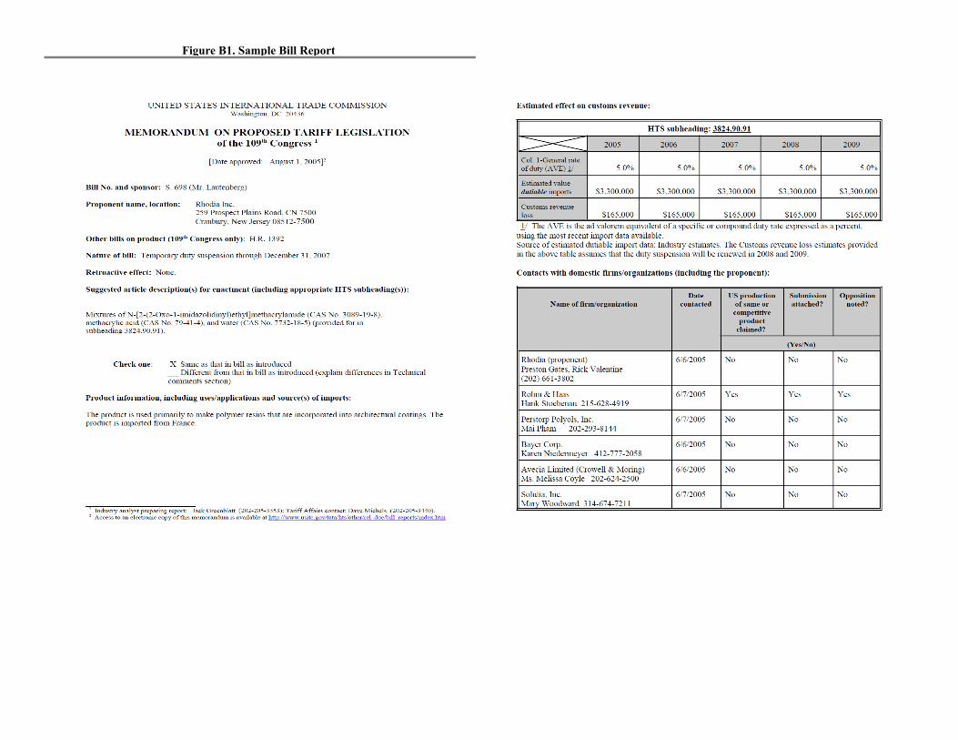
Figure B1. Sample Bill Report

Figure B2. Sample Lobbying Report - 3M Company