Embed Size (px)
Citation preview

Project ID: NTC2016-SU-R-07
PROTECTING GLOBAL MARITIME-BASED
INTERMODAL FREIGHT DISTRIBUTION SYSTEMS
FROM THE IMPACTS OF CLIMATE CHANGE
Final Report
by
Elise Miller-Hooks
George Mason University
Ali Asadabadi
Graduate Research Assistant
George Mason University
for
National Transportation Center at Maryland (NTC@Maryland)
1124 Glenn Martin Hall
University of Maryland
College Park, MD 20742
March 15, 2018


iii
ACKNOWLEDGEMENTS
This project was funded by the National Transportation Center @ Maryland (NTC@Maryland),
one of the five National Centers that were selected in this nationwide competition, by the Office
of the Assistant Secretary for Research and Technology (OST-R), U.S. Department of
Transportation (US DOT).
DISCLAIMER
The contents of this report reflect the views of the authors, who are solely responsible for the
facts and the accuracy of the material and information presented herein. This document is
disseminated under the sponsorship of the U.S. Department of Transportation University
Transportation Centers Program in the interest of information exchange. The U.S. Government
assumes no liability for the contents or use thereof. The contents do not necessarily reflect the
official views of the U.S. Government is report does not constitute a standard, specification, or
regulation.

v
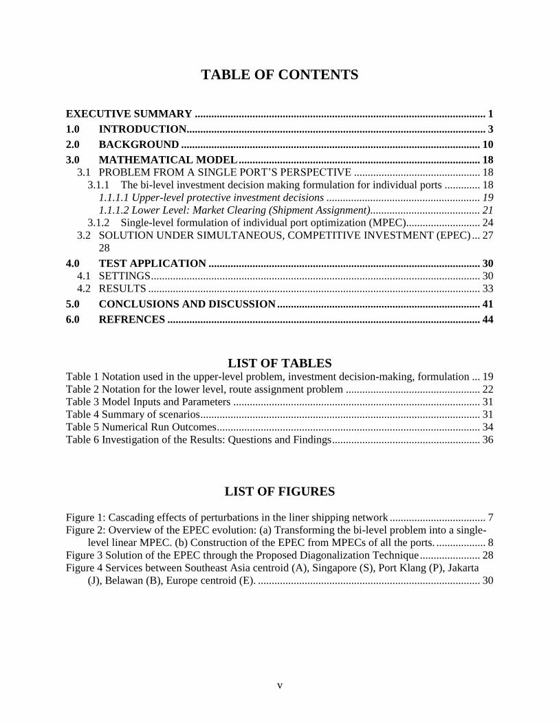
TABLE OF CONTENTS
EXECUTIVE SUMMARY .......................................................................................................... 1
1.0 INTRODUCTION............................................................................................................. 3
2.0 BACKGROUND ............................................................................................................. 10
3.0 MATHEMATICAL MODEL ........................................................................................ 18 3.1 PROBLEM FROM A SINGLE PORT’S PERSPECTIVE .............................................. 18
3.1.1 The bi-level investment decision making formulation for individual ports ............. 18 1.1.1.1 Upper-level protective investment decisions ........................................................ 19
1.1.1.2 Lower Level: Market Clearing (Shipment Assignment)........................................ 21 3.1.2 Single-level formulation of individual port optimization (MPEC)........................... 24
3.2 SOLUTION UNDER SIMULTANEOUS, COMPETITIVE INVESTMENT (EPEC) ... 27
28
4.0 TEST APPLICATION ................................................................................................... 30 4.1 SETTINGS ........................................................................................................................ 30 4.2 RESULTS ......................................................................................................................... 33
5.0 CONCLUSIONS AND DISCUSSION .......................................................................... 41
6.0 REFRENCES .................................................................................................................. 44
LIST OF TABLES Table 1 Notation used in the upper-level problem, investment decision-making, formulation ... 19
Table 2 Notation for the lower level, route assignment problem ................................................. 22
Table 3 Model Inputs and Parameters .......................................................................................... 31
Table 4 Summary of scenarios ...................................................................................................... 31
Table 5 Numerical Run Outcomes ................................................................................................ 34
Table 6 Investigation of the Results: Questions and Findings ...................................................... 36
LIST OF FIGURES
Figure 1: Cascading effects of perturbations in the liner shipping network ................................... 7 Figure 2: Overview of the EPEC evolution: (a) Transforming the bi-level problem into a single-
level linear MPEC. (b) Construction of the EPEC from MPECs of all the ports. .................. 8
Figure 3 Solution of the EPEC through the Proposed Diagonalization Technique ...................... 28 Figure 4 Services between Southeast Asia centroid (A), Singapore (S), Port Klang (P), Jakarta
(J), Belawan (B), Europe centroid (E). ................................................................................. 30

1
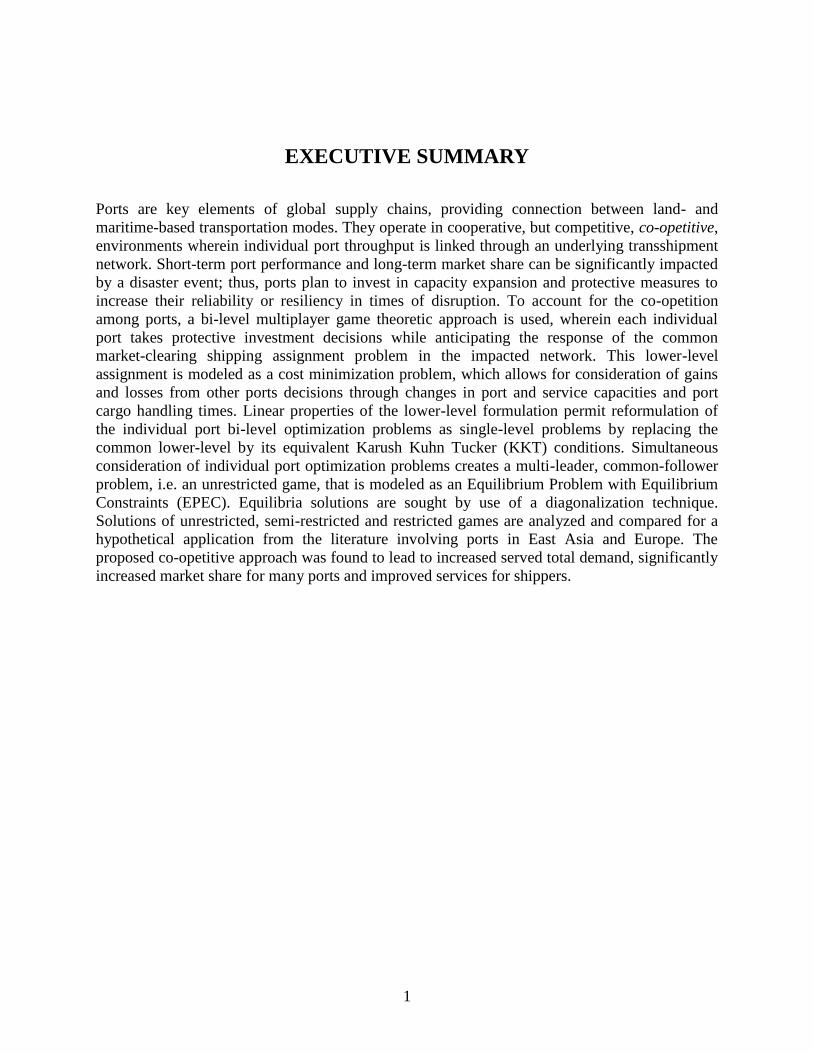
EXECUTIVE SUMMARY
Ports are key elements of global supply chains, providing connection between land- and
maritime-based transportation modes. They operate in cooperative, but competitive, co-opetitive,
environments wherein individual port throughput is linked through an underlying transshipment
network. Short-term port performance and long-term market share can be significantly impacted
by a disaster event; thus, ports plan to invest in capacity expansion and protective measures to
increase their reliability or resiliency in times of disruption. To account for the co-opetition
among ports, a bi-level multiplayer game theoretic approach is used, wherein each individual
port takes protective investment decisions while anticipating the response of the common
market-clearing shipping assignment problem in the impacted network. This lower-level
assignment is modeled as a cost minimization problem, which allows for consideration of gains
and losses from other ports decisions through changes in port and service capacities and port
cargo handling times. Linear properties of the lower-level formulation permit reformulation of
the individual port bi-level optimization problems as single-level problems by replacing the
common lower-level by its equivalent Karush Kuhn Tucker (KKT) conditions. Simultaneous
consideration of individual port optimization problems creates a multi-leader, common-follower
problem, i.e. an unrestricted game, that is modeled as an Equilibrium Problem with Equilibrium
Constraints (EPEC). Equilibria solutions are sought by use of a diagonalization technique.
Solutions of unrestricted, semi-restricted and restricted games are analyzed and compared for a
hypothetical application from the literature involving ports in East Asia and Europe. The
proposed co-opetitive approach was found to lead to increased served total demand, significantly
increased market share for many ports and improved services for shippers.

2

3
1.0 INTRODUCTION
Maritime transport operating within Intermodal (IM) freight distribution systems remain the
dominant mode for international trade (International Maritime Organization,
https://business.un.org/en/entities/13). It plays a significant role in the U.S. and world economies,
serving as the backbone to global trade and supply chain networks. Ports are critical components
of these systems, providing key land-water connections. However, they are vulnerable to
disruptive impacts from a range of anthropogenic and natural hazard causes, including tsunamis,
earthquakes, meteorological events, terrorism, worker strikes and operational accidents.
Moreover, damage, disruptions, backups, or physical, administrative or operational changes that
arise in a single port can affect the performance of other ports, along with the overall system.
Consider for example an event arising at a single port that impacts its throughput capacity. In
addition to a shortage in berth space for incoming vessels, vessels will be delayed from moving
to the next location, in turn creating queues and additional upstream backups and downstream
delays. An initial disruption, thus, causes delays that ripple through the network, impacting other
ports’ operations and system-level productivity. This ripple effect in the maritime network is
depicted in Error! Reference source not found. where a disruption in one port leads to delays
at other ports along the shipping routes.
In this competitive environment, disruptions can lead to significant immediate losses in revenue
and ultimate market share, as alternative competing ports can serve diverted traffic. This is
especially problematic in transshipment operations, where interchange locations are replaceable,
and traffic diversion can lead to a rebalancing of revenues across the port network. The
4
disruptions, thus, affect the long-term competitive position of affected ports, potentially
preventing them from regaining their pre-disaster market share even after capacity is completely
restored (Chang 2000). If such disruptions occur frequently enough, whether or not due directly
to events at a specific port, the delays will impact the ports’ reliability and thus its reputation.
Many shipping companies directly or indirectly account for potential delays and resulting losses
in choosing their IM routes. Ports are, therefore, incentivized to make pre-disaster mitigative and
preventative investments to reduce vulnerabilities for the purpose of maintaining and increasing
their market share (Song & Panayides 2012). This is also important to manufacturers and
suppliers that rely on the IM network to ship or receive their goods and materials. Companies
relying on raw materials or parts will direct shippers to consider multiple alternative routes in
case of port disruptions to avoid delays in manufacturing (Tang 2006).
An individual port authority can invest in its own facilities to protect its business from the threats
of disruptions and more major disaster events. These investments may involve pre-event
enhancements (e.g. reinforcing or raising a wharf or pier, raising roadway and railway elements,
redesigning drainage systems, building coastal defenses, soil strengthening, seismic design,
facility retrofit, installation of security systems,…), post-event repair, or improvements in
equipment, insurance coverage, and personnel training. Pre-event preparedness is especially
important where post-disaster actions may be inadequate for the disaster event category (Chang
2000). While such investments are important, they do not guarantee performance, because a
port’s fate is a function of its place within the larger shipping network. A disruption in one port
node of this maritime network can affect the continuation/disruption or gains/losses at other
network elements. Thus, protective investments must aim to guard against or enable adaptive
action for both on-site events and events at interconnected facilities within the maritime network,

5
and benefits may be derived from investing in others’ facilities. The protective investment
problem exists, thus, in a cooperative and simultaneously competitive, co-opetitive, environment
wherein each port can anticipate its competitors’ investment decisions and consider potential
gains from collaboration. The term co-opetition was introduced by Nalebuff et al. (1996) in the
context of business management.
The global maritime-port network involves a range of stakeholders from national, state and
private sectors. Ports may be publically or privately owned, and may be operated by the same or
different public or private parties (Brooks 2004). In this co-opetitive IM environment, each
stakeholder is interested in not only the well-being of its own facilities, but also in other facilities
within its maritime network. This complicates the process of analyzing and optimizing
preventative or response-related investments to disruption events. A co-opetitive optimization
scheme not previously considered in the literature in this context is proposed herein for this
purpose. This scheme supports the development of decentralized, yet cooperative investment
strategies.
This multi-stakeholder, protective investment problem for ports operating within a competitive
but connected IM network is conceptualized as a multi-player, bi-level investment problem.
Decisions by a player to invest in its own or other’s facilities are taken individually at the upper
level of the bi-level formulation while anticipating solution of a common liner shipping
assignment at the lower level. The ports’ objectives are to maximize their own throughput (i.e.
profit) by protecting from impacts of disruption events across the port network. Given post-event
route capacities and traversal times, the liner shipping problem assigns container shipping
demand to the functioning routes; that is, it recalibrates market response to disrupted transport
options.

6
1
2
3
Ports
Initial Disruption First-tier disrupted ports Second-tier disrupted ports
Links, disrupted links
7
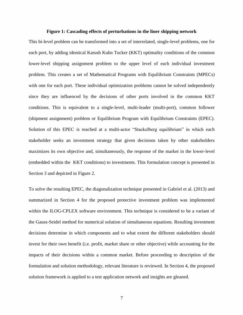
Figure 1: Cascading effects of perturbations in the liner shipping network
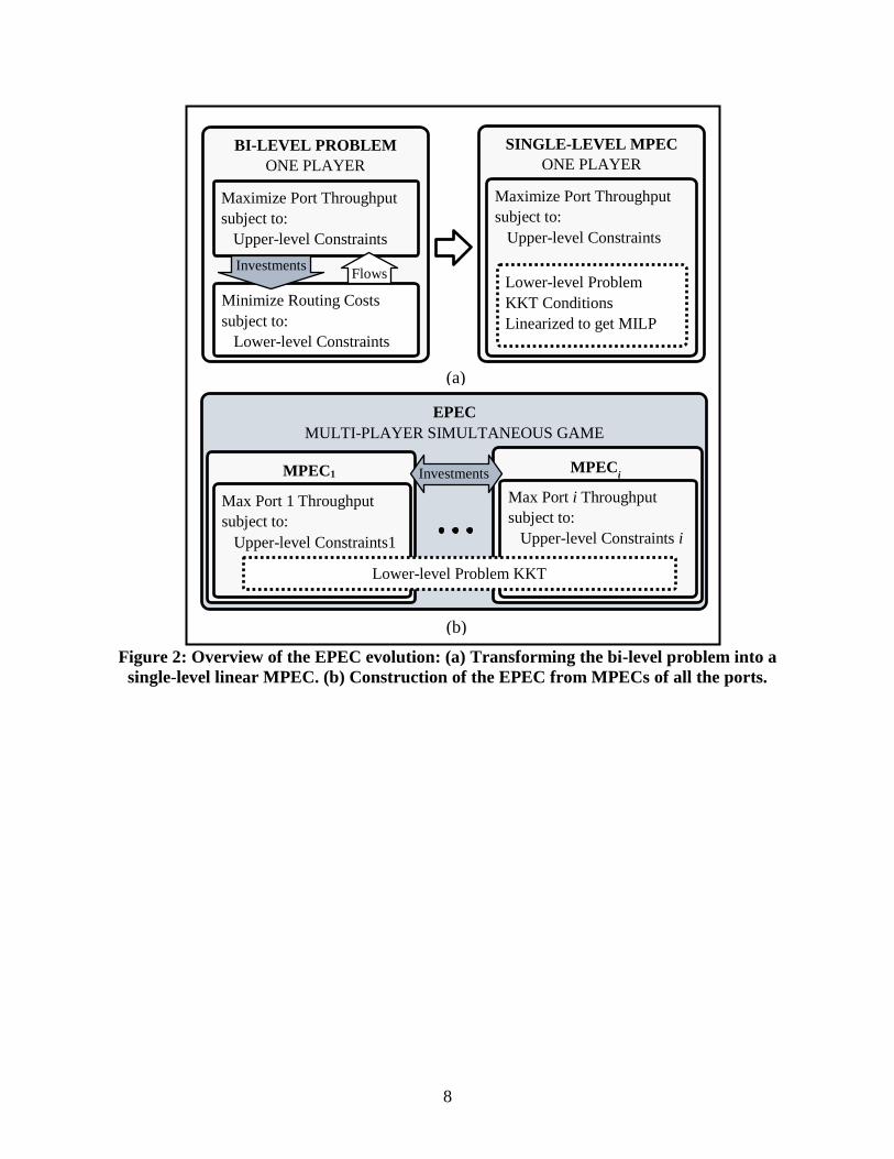
This bi-level problem can be transformed into a set of interrelated, single-level problems, one for
each port, by adding identical Karush Kuhn Tucker (KKT) optimality conditions of the common
lower-level shipping assignment problem to the upper level of each individual investment
problem. This creates a set of Mathematical Programs with Equilibrium Constraints (MPECs)
with one for each port. These individual optimization problems cannot be solved independently
since they are influenced by the decisions of other ports involved in the common KKT
conditions. This is equivalent to a single-level, multi-leader (multi-port), common follower
(shipment assignment) problem or Equilibrium Program with Equilibrium Constraints (EPEC).
Solution of this EPEC is reached at a multi-actor “Stackelberg equilibrium” in which each
stakeholder seeks an investment strategy that given decisions taken by other stakeholders
maximizes its own objective and, simultaneously, the response of the market in the lower-level
(embedded within the KKT conditions) to investments. This formulation concept is presented in
Section 3 and depicted in Figure 2.
To solve the resulting EPEC, the diagonalization technique presented in Gabriel et al. (2013) and
summarized in Section 4 for the proposed protective investment problem was implemented
within the ILOG-CPLEX software environment. This technique is considered to be a variant of
the Gauss-Seidel method for numerical solution of simultaneous equations. Resulting investment
decisions determine in which components and to what extent the different stakeholders should
invest for their own benefit (i.e. profit, market share or other objective) while accounting for the
impacts of their decisions within a common market. Before proceeding to description of the
formulation and solution methodology, relevant literature is reviewed. In Section 4, the proposed
solution framework is applied to a test application network and insights are gleaned.
8
Figure 2: Overview of the EPEC evolution: (a) Transforming the bi-level problem into a
single-level linear MPEC. (b) Construction of the EPEC from MPECs of all the ports.
EPEC
MULTI-PLAYER SIMULTANEOUS GAME
BI-LEVEL PROBLEM
ONE PLAYER
(a)
(b)
Minimize Routing Costs
subject to:
Lower-level Constraints
SINGLE-LEVEL MPEC
ONE PLAYER
Maximize Port Throughput
subject to:
Upper-level Constraints
Lower-level Problem
KKT Conditions
Linearized to get MILP
Maximize Port Throughput
subject to:
Upper-level Constraints
MPEC1
Max Port 1 Throughput
subject to:
Upper-level Constraints1
MPECi
Max Port i Throughput
subject to:
Upper-level Constraints i
Lower-level Problem KKT
Investments Flows
Investments

9

10
2.0 BACKGROUND
Supply chain risk management has been extensively studied. In this context, risk is typically
defined with respect to reoccurring (e.g. operational) or rarer catastrophic disruptions that impact
some aspect of the supply chain. Only a few such works explicitly consider the role of
transportation in supply chain risk. Ho et al. (2015), in their comprehensive review on supply
chain risk management, list only one work (Hishamuddin et al., 2013) that accounts for
transportation risks in supply chains. Hishamuddin et al. focus on recovery scheduling related to
ordering and production; they do not investigate potential protective investments to reduce this
transportation risk. Rienkhemaniyom and Ravindran (2014) mathematically modeled a multi-
objective supply chain network design problem involving risks associated with disruptions at
facilities and transportation links. Their model seeks decisions on the design of the supply chain,
including decisions related to the selection of suppliers, manufacturing plants, and distribution
centers, as well as plans for production and distribution. They propose the use of goal
programming to seek optimal or satisficing design solutions in terms of network performance
and risk attributes. Loh and Van Thai (2014) discuss the increasingly important role of ports in
the global supply chain network. They note that very few works have focused on the
management of port disruptions as part of the supply chain. Thus, this remains an open area.
Effective investment decision making for improved resiliency requires a deep understanding of
the system-level impacts of port disruptions. Some works have sought to describe how
disruptions cascade through the supply chain network. Wu et al. (2007) studied the propagation
of disruptions in supply chains and their impacts on the network. They used a technique they
11
termed Disruption Analysis Network for this purpose. This technique models the supply-chain
interconnections using an underlying directed bipartite graph. Using this graph-based
representation, the impact of simulated disruption events can be estimated with respect to
important network attributes. Sokolov et al. (2016) proposed a two-model, multi-criteria
approach for use in supply chain design that captures the ripple effects of disruptions. The model
accounts for static structural properties of the supply chain through the use of graph theory
concepts. The static model is extended to include time-dependent characteristics needed to
understand the dynamic effects of disruptions. These effects are interpreted as an indicator of
design robustness.
The use of “Systemigrams” is suggested in Mansouri et al. (2009) for studying the effects of
disruptions in a multi-agent maritime transportation system of ships, ports, intermodal
connections, waterways and users. This tool enables the various stakeholders of the supply chain,
from the manufacturers to the retail stores, to create qualitative understanding of the
perspectives, organizational requirements and strategies of other stakeholders. This tool is aimed
at supporting a participatory environment by elucidating interdependencies. Rose and Wei
(2013) studied direct and indirect effects of port disruptions on regional and national economies
using an input-output (I-O) (demand-supply) macroscopic approach. Resiliency of the economy
as a function of inventories, re-routing, overtime and extra shifts is incorporated.
The literature is replete with qualitative works and reviews that consider threats to ports,
their resiliency, decision-making practices and their impacts on the global supply chain network.
Becker et al. (2012) conducted a comprehensive survey of port authorities around the world.
They investigated the current knowledge, perceptions and planning efforts among seaport
administrators to address the impacts of climate change. The authors found that by and large the

12
respondents did not plan for climate change. Moreover, they planned for a period of less than 10
years, despite that their infrastructure decisions may have century-long impacts. They noted that
the respondents were in agreement about the importance of addressing the potential
consequences of climate change, but felt uninformed. Shaw et al. (2016) explored the multi-level
structure of port resilience planning, including government departments, port operators,
importers, agents and logistic firms. They suggest that this complex system requires information
sharing between stakeholders for preparation for disasters. Python and Wakeman (2016) review
some of the lessons learned from post-super storm Sandy at the ports of New York and New
Jersey. They concluded that ports must address the risks of climate change impacts. They argue
that if ports are willing to overcome the competitiveness and share information during
disruptions, they can increase their own resiliency, as well as ensure the resiliency of the supply
chain.
Some works focus on resiliency modeling, quantification and optimization for an individual port.
These works model detailed port operations. The output of their models can be used to create
performance curves for scenario generation in this study. Nair et al. (2010) applied a resilience
quantification and enhancement framework proposed in (Chen & Miller-Hooks 2012) to ports.
They built a detailed network model of port operations for a port in Poland and used a
throughput ratio based on satisfied demand as their resiliency measure. They considered five
categories of hazard events for generating thousands of potential disruption scenarios and
suggested a host of recovery actions for recapturing lost operational capacity under a multi-
hazard stochastic framework. They measure resiliency in terms of both the inherent coping
capacity and adaptability as a function of recovery action. Shafieezadeh and Ivey Burden (2014)
introduced a framework for quantification of seismic resiliency of a seaport. They used the
13
integral of post-disruption performance over time to measure network resiliency. Yang et al.
(2015) used a fuzzy risk analysis approach to evaluate the economic impact of adaptation
policies for port resiliency. Using fuzzy set theory, they combine linguistic data on climate
change risk parameters (timeframe, likelihood, severity of consequences) to produce fuzzy safety
score. They estimate the potential risk reduction and cost-effectiveness of considered adaptation
strategies.
A few studies assessed the resiliency of a networked system of ports. Omer et al. (2012) studied
the resiliency of maritime transportation systems using a proposed Networked Infrastructure
Resiliency Assessment (NIRA) framework. They suggest three resiliency metrics: tonnage, time
and cost resiliency. They quantified the impact of disruptions on two connected ports using a
system dynamics model to account for the impact of a reduction in capacity of the receiving port
on shipping times. They evaluated the benefits of alternative in-land connections on the
resiliency metrics for the two ports. Achurra-Gonzalez et al. (2016) used a cost-based container
flow assignment method (presented in Bell et al., 2013) to investigate the role of capacity
reduction in ports in redistribution of cargo flows due to changing route costs. Angeloudis et al.
(2007) examined the properties of the liner-container shipping network using concepts of graph
theory. They found the network to be scale-free, wherein some nodes have exceptionally high
degree compared to the majority of nodes, and detected the busiest nodes in the network. They
examined the responsiveness of the network to events that impair network elements (nodes)
through rerouting the container ships. They concluded that the critical nodes of the network are
not necessarily the busiest ones, and the impacts on processing of shipments at other ports is
highly variable. Peng et al. (2016) formulate a centralized version of the protective investment
decision problem for the liner shipping network as a two-stage stochastic program given
14
randomly arising disruption events. While related to this work, Peng et al.’s work presumes that
a single authority can invest across the network using a common budget. Such a system-optimal,
centralized investment strategy can provide a bound on network-wide performance under a
social, shipping cost minimizing, objective.
Although a number of works have studied the reliability or resiliency of port networks, either
from a graph theory viewpoint (Angeloudis et al. 2007) or by examining throughput before and
after disruptions (Achurra-Gonzalez et al., 2016; Angeloudis et al., 2007; Peng et al., 2016;
Omer et al., 2012), all considered protective investment decisions to be made centrally under a
single, common budget. In reality, the ports are not managed centrally, and in fact are competing
and cooperating to increase their own market shares.
A number of studies have modeled competition between two ports through setting of handling
costs (port charges) for shippers, expansion and service-choice strategies, and sometimes by
seeking to impact port-of-call decisions. Ishii et al. (2013) constructed a non-cooperative, two-
player game for setting port charges given port capacity expansion plans and demand
uncertainty. Asgari et al. (2013) model a game among two competing hub ports for setting port
charges. Shipping companies, acting as the leader, choose the lowest cost option. They use a
utility function to model the attractiveness of each hub port to the shipping companies and
embed the utility function within an objective through which the ports respond to shipper
decisions at the lower level. Song et al. (2016a) model a two-level game among two liner
shipping companies. Similar to Asgari et al., Song et al. model port-call decisions by two
competing shipping companies (the leaders) at the upper level and port charge settings by two
ports (followers) in the lower level. Song et al. (2016b) for a similar problem propose a two-
player (two-ports) game in which payoffs of the game are assessed through the benefits to a
15
single ocean carrier choosing a port-of-call. They mathematically derived the equilibrium
solution to this simplified game. Chen and Liu (2016) use a two-player game to model expansion
investment decisions of two ports considering congestion and uncertain market demand. Zhuang
et al. (2014) also present a two-player game for two ports considering service-choice decisions
and derive the equilibrium solution mathematically for their specialized problem. Other works
have multiplayer, bi- or tri-level structures also related to port charge decision (Lee et al., 2014;
Lee et al., 2014a; Lee and Choo, 2016; Zhang et al., 2009). These works anticipate shipper
routing decisions in the lower level response.
Other relevant works arise in the broader field of infrastructure investment that also apply a two-
or more-player (game theoretic) approach. Reilly et al. (2015) model investment decision making
for interdependent infrastructure networks as a game. They provide a general formulation that
associates investments and payoffs for two players and compare solutions under a simultaneous
game, sequential game, and social optimum. They discuss the application of the two-player game
theory approach for flood protection investment planning. Of greater relevance to supply chains
is work by Bakshi and Kleindorfer (2009). They used a Harsanyi-Selten-Nash bargaining
framework to model mitigative investments of two participants in a supply chain. They study
tradeoffs between pre-event mitigative investment sharing and post-event loss-sharing net of
insurance payouts. Bakshi and Mohan (2015) studied mitigation of cascading disruptions in
supply networks. They found that investments and payoffs of a firm are dependent on at most its
tier-2 suppliers. Finally, Do et al. (2015) used a game theoretic approach to investigate
competition between two ports in investing for expansion given uncertain demand. They
estimated that profits enabled through expansion and ensuing increase in market share were
highly dependent on the actions of other ports in the maritime network. These works are relevant
16
here in their game-theoretic approaches, and their recognition of the importance of understanding
the ramifications of a port’s decisions given its place within an interconnected port network.
The few works that consider a multi-player scheme in the context of infrastructure resiliency and
reliability (Bakshi and Kleindorfer, 2009; Reilly et al., 2015; Bakshi and Mohan, 2015; Do et al.,
2015) are generic, using Nash games of only two investors under simplified investment strategies
and payoff schemes.
The work herein offers a multi-leader, common-follower structure, i.e. an EPEC formulation,
that enables a realistic representation of the co-opetitive environment in which multiple ports
operating within a maritime network involving shippers must make their investment decisions.

17
18
3.0 MATHEMATICAL MODEL
The multi-stakeholder, protective port investment problem is formulated in this section. First,
though, the single-player version, an MPEC, which takes the perspective of an individual port
investing in isolation, is presented.
3.1 PROBLEM FROM A SINGLE PORT’S PERSPECTIVE
A single port can make pre-disaster investments with the aim of maintaining or quickly
reclaiming capacity during or after a disruption event. In addition to retaining its current market
share, the port, through its investments, may be poised to capture a larger portion of the shipping
market. In this subsection, the protective investment problem is formulated taking this single-
port perspective.
3.1.1 The bi-level investment decision making formulation for individual
ports
The single-player protective investment problem is formulated as a bi-level problem in which a
port (leader) makes protective investment decisions at the upper-level while anticipating the
response of a lower-level problem. The lower-level problem corresponds to the market clearing
shipping assignment problem. Throughput maximization is sought in the upper level, while
shippers (the followers) seek lowest cost routes in the lower level. Solution is obtained at a
Stackelberg equilibrium wherein investments are optimal for the given market response. This
structure is presented in Figure 2(a).

19
1.1.1.1 Upper-level protective investment decisions
In the upper-level, investment decisions are made from the perspective of a port authority with
the goal of mitigating the impacts of a disruption event and preventing the loss of business to
competing, unaffected or better prepared ports. Notation used in formulating the upper level
along with the upper-level formulation for two perspectives are given next. The response at the
lower level is presented in the next subsection.
Table 1 Notation used in the upper-level problem, investment decision-making,
formulation
Sets Subsets Indices
Legs Legs entering port Legs
Origin ports Legs leaving port Ports
Destination ports Origin ports
All ports Destination ports
Parameters
Budget of port
Decision variables
Investments of port in port (parameters to the lower-level problem),
Flow of containers on leg en route to destination , where a leg is a specific transit task
between two ports Flow of containers from origin to destination
Optimization from Port ’s perspective:
(1)
Subject to:
(2)
(3)
The objective as given by (1) seeks to maximize total container traffic, including inbound,
outbound and transshipment traffic. To avoid double-counting, only inbound movements of the
transshipments are counted. Added revenue generated through sea-to-land container handling
can be included through an additional term if desired. The penalty term, , is added to

20
the objective to ensure that port i only invests when the investment leads to additional
throughput. must be smaller than the marginal value of processing one additional container.
Budget limitations are given in Constraint (2). Investments by port i must be nonnegative
(Constraints (3)). Flows along the legs ( for and ) are set in conjunction with
solution of the lower-level problem described in the next subsection.
An alternative objective function that captures the trade-offs between protective investments and
loss of shipping business might be considered:
(4)
where converts port throughput to a monetary value. With such a profit-based objective, both
the budget constraint (4) and the term in (4) can be eliminated.
System perspective (maximize welfare)
Taking a centralized decision-making approach, the objective is given in terms of maximizing
total port throughput in the maritime network wherein port investments, , across the network
are allocated from a common, pooled budget for the benefit of social welfare. A centralized
approach is commonly taken in the literature. While it may benefit the shippers, this may not be
the case for the individual ports.
(5)
Subject to:
(6)
(7)

21
1.1.1.2 Lower Level: Market Clearing (Shipment Assignment)
The decisions of port authorities to invest in mitigative actions are based on the anticipated
response from the underlying shipping network reflected in the lower-level assignment problem.
The impacts of a disaster scenario given protective, port-level investments determine the
port/route capacities and processing/traversal times in the network. For the lower-level problem,
a cost-based routing assignment formulation is adopted from Achurra-Gonzalez et al. (2016) (for
a review on liner shipping and container routing optimization the reader is referred to Tran and
Haasis, 2015). Where possible, notation follows that given in this earlier work.
A pre-defined set of services with associated links and legs model the liner-shipping network.
Containers are assigned to legs such that costs of handling, renting and depreciation due to cargo
transfer or dwell times are minimized. Note that each unit of shipment involves handling at the
two ends of its trip; thus, Achurra-Gonzalez et al. assign higher handling costs to leg ends that
occur at shipment origins and destinations. Legs representing movements between transshipment
nodes are assumed to require modest handling costs at their end points. Any handling cost above
this is considered extra. If the sum of extra handling costs for legs connecting origin-destination
(o-d) pairs is equal to the sum of extra costs of handling for legs between origins and
transshipment nodes and between transshipment nodes and destinations, as is the case in
Achurra-Gonzalez et al. (2016), the total handling cost for each container would only depend on
the number of legs used in its shipment, and the extra handling costs will be equal in any feasible
combination of legs. Thus, leg types as used in their formulation are unnecessary and their
formulation can be simplified without loss. This previous work considered only a single o-d pair;
however, the proposed simplification is required in applications with multiple o-d pairs. This is

22
because the leg type is defined for only one o-d pair, while containers in the same ship may have
different origins and destinations.
Table 2 Notation for the lower level, route assignment problem
Sets Subsets Indices
Legs Legs entering port Legs
Origin ports Legs leaving port Origin ports
Destination ports Legs on route Destination ports
All ports Links on route Ports
All routes Ports on route Routes
All links Links
Parameters
Sailing time on leg , including port loading and unloading times, without improvements from
pre-disaster investments
Investments of port in port for
Capacity loss reduction due to disaster event per unit investment in port
Capacity loss reduction due to disaster event per unit investment in any port on route r
Reduction in traversal time increase due to disaster event per unit investment in any port on
leg
Ratio of effectiveness of internal to external investment
Container handling cost per container for a leg on route
Per container rental and depreciation cost (inventory cost) per unit time
Containers to be transported from origin to destination
1 if leg uses link on route , 0 otherwise
Frequency of sailing on leg
Post-disaster capacity of route
Post-disaster maximum throughput capacity at port
Penalty cost for containers not transported
Decision variables
Flow of containers from origin to destination
Flow of containers on leg en route to destination
Dual variables
(8)
Subject to:
23
(9)
(10)
(11)
(12)
(13)
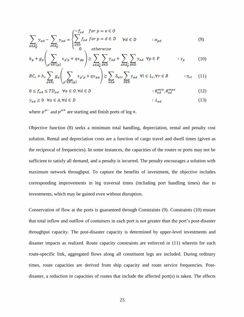
where and are starting and finish ports of leg .
Objective function (8) seeks a minimum total handling, depreciation, rental and penalty cost
solution. Rental and depreciation costs are a function of cargo travel and dwell times (given as
the reciprocal of frequencies). In some instances, the capacities of the routes or ports may not be
sufficient to satisfy all demand, and a penalty is incurred. The penalty encourages a solution with
maximum network throughput. To capture the benefits of investment, the objective includes
corresponding improvements in leg traversal times (including port handling times) due to
investments, which may be gained even without disruption.
Conservation of flow at the ports is guaranteed through Constraints (9). Constraints (10) ensure
that total inflow and outflow of containers in each port is not greater than the port’s post-disaster
throughput capacity. The post-disaster capacity is determined by upper-level investments and
disaster impacts as realized. Route capacity constraints are enforced in (11) wherein for each
route-specific link, aggregated flows along all constituent legs are included. During ordinary
times, route capacities are derived from ship capacity and route service frequencies. Post-
disaster, a reduction in capacities of routes that include the affected port(s) is taken. The effects

24
of investments aimed at countering disaster impacts are also included. Together, Objective (8)
and Constraints (10) and (11) model the reductions in port and route-level capacities and
increased traversal/handling costs due to the disaster event, as well as the effectiveness of pre-
event investment actions. Objective (8) and Constraints (10) and (11) can be revised to model
investment benefits in traversal time and port and route capacities that are attained only in the
event of disruption. Constraints (12) enforce the OD flows to be between 0 and a total fixed
demand.
3.1.2 Single-level formulation of individual port optimization (MPEC)
The upper- and lower-level problems together create the bi-level investment optimization
problem for a single port decision-maker operating within a larger maritime network. This can be
summarized as the following mathematical problem:
Max (1)
subject to:
(2) and (3)
Min (8)
subject to:
(9)-(13)
To facilitate the reformulation of port ’s investment problem in a single level, the lower-level
problem, (8)-(13), can be replaced by its KKT conditions. Since the lower-level problem is
linear, the KKT conditions are necessary and sufficient for optimality, and the problem reduces
to a MPEC (Figure 2(a)) as given next.

25
MPEC for port
(1)
Subject to:
(2)
(3)
(14)
(15)
(9)
(16)
(17)
(18)
(19)
(20)
where is service route of leg .
Constraints (2) and (3) are upper-level constraints while (9) and (14)-(20) are lower-level KKT
conditions including the equality, inequality, complementary slackness and non-negativity
constraints. By way of example, the function with respect to constraint (19) operates as:
, a lower-level inequality , non-negativity of the dual variable

26
, complementarity slackness
A disjunctive constraints approach (Fortuny-Amat & McCarl 1981) is applied in creating
equivalent linear constraints for complementarity equations (16)-(20), resulting in reformulation
of the MPEC as a Mixed Integer Program (MIP). As an example, for constraints (19):
,
where and are large values that place no restrictions on and when K is
1 or 0, respectively. On the other hand, if the s are set unnecessarily large, they will expand the
feasibility region and significantly increase MIP solution time. For primal variables, the selection
of these values can relate to the application. The setting of these values for the dual variables,
however, is less intuitive and may require trial-and-error. In the context of this model, can be
set within a small increment above the associated maximum o-d flow or port or route capacity. In
some cases, the setting of can be guided by insights gleaned from the shadow prices of the
lower-level problem. In all cases, they must be larger than (roughly equal to or slightly more than
double) the value of the penalty cost, PC, applied within the KKT constraints associated with the
lower-level objective function.
By employing this linear equivalent model, optimality of the individual MPECs is guaranteed.
Moreover, this approach increases the speed of convergence of the proposed diagonalization
method described in the next section.
27
3.2 SOLUTION UNDER SIMULTANEOUS, COMPETITIVE
INVESTMENT (EPEC)
Simultaneous consideration of the MPECs associated with each of the ports creates a single
EPEC which produces an equilibrium solution on the investment decisions (Figure 2(b)). To
solve this EPEC, the well-known diagonalization technique (see Gabriel et al., 2013 for
additional background) is employed here (Error! Reference source not found.Figure 3). This
technique can be described in terms of the following main steps.
1- Initial investment decisions are selected. A multi-start technique is commonly
implemented and will potentially produce multiple equilibria.
2- The individual port protective investment problem is solved assuming fixed
investment decisions for all other ports, and investment decisions are updated before
proceeding to solve the individual problem for the next port. This is repeated until all
individual port problems are solved once.
3- Step 2 is repeated until the investment decisions converge. Convergence is achieved
when the difference between the results of two consecutive iterations are less than a
defined threshold.
For a network with ports, service routes, legs, links, OD pairs and destinations, the
MPEC for one port is a MIP with continuous variables,
binary variables (for disjunctive constraints) and
constraints. Solution times also depend on the big
settings. Note that the problem size does not depend on the characteristics of the considered
disaster scenario. While convergence of the diagonalization technique for solving the larger

28
EPEC is not guaranteed, it was found to work well (generally achieved within three to six
iterations of the whole process and 20 iterations in the worst case) in this application (Section 4).
Figure 3 Solution of the EPEC through the Proposed Diagonalization Technique
One might solve this problem by constructing the EPEC through simultaneous consideration of
the KKT conditions of all the individual MPECs in one grand problem. To achieve this, an
equivalent single-level MPEC can be derived for each player by moving constraints of the lower
level to the upper level and adding corresponding dual constraints and strong duality conditions
to ensure that solutions meet primal-dual optimality. To solve the combined set of single-level
MPECs, the KKT conditions of each MPEC can be incorporated within a single program.
Solution of this grand problem is obtained at a multi-player equilibrium. This approach,
Initialize
investment
decisions for all
ports:
Have all port-level investments
converged?
yes
If convergence achieved,
set equilibrium investment
decisions:
No
Solve MPEC1
assuming fixed
for all
Solve MPEC2
assuming fixed
for all
Solve MPECj
assuming fixed
for all

29
however, requires convexity of each MPEC for KKT condition sufficiency, which was not
present.

30
4.0 TEST APPLICATION
4.1 SETTINGS
The framework was tested on 6-node maritime network representation of ports presented in
(Achurra-Gonzalez et al., 2016). Network nodes correspond to four East Asian ports and two
clusters of ports at the centroids of Europe and Asia. As depicted in Figure 4, network nodes are
connected through five service routes. Port and route capacities, route frequencies, port budgets,
o-d demand and handling, rental, depreciation and penalty costs are all listed in Table 3.
Figure 4 Services between Southeast Asia centroid (A), Singapore (S), Port Klang (P),
Jakarta (J), Belawan (B), Europe centroid (E).
31
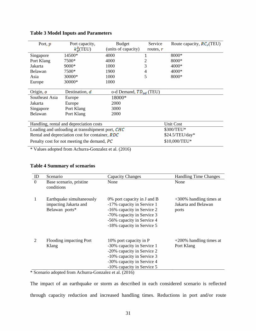
Table 3 Model Inputs and Parameters
Port, Port capacity,
(TEU)
Budget
(units of capacity)
Service
routes,
Route capacity, (TEU)
Singapore 14500* 4000 1 8000*
Port Klang 7500* 4000 2 8000*
Jakarta 9000* 1000 3 4000*
Belawan 7500* 1900 4 4000*
Asia 30000* 1000 5 8000*
Europe 30000* 1000
Origin, Destination, o-d Demand, (TEU)
Southeast Asia Europe 18000* Jakarta Europe 2000
Singapore Port Klang 3000
Belawan Port Klang 2000
Handling, rental and depreciation costs Unit Cost
Loading and unloading at transshipment port, $300/TEU*
Rental and depreciation cost for container, $24.5/TEU/day*
Penalty cost for not meeting the demand, $10,000/TEU*
* Values adopted from Achurra-Gonzalez et al. (2016)
Table 4 Summary of scenarios
ID Scenario Capacity Changes Handling Time Changes
0 Base scenario, pristine
conditions
None None
1 Earthquake simultaneously
impacting Jakarta and
Belawan ports*
0% port capacity in J and B
-17% capacity in Service 1
-16% capacity in Service 2
-70% capacity in Service 3
-56% capacity in Service 4
-18% capacity in Service 5
+300% handling times at
Jakarta and Belawan
ports
2 Flooding impacting Port
Klang
10% port capacity in P
-30% capacity in Service 1
-20% capacity in Service 2
-10% capacity in Service 3
-30% capacity in Service 4
-10% capacity in Service 5
+200% handling times at
Port Klang
* Scenario adopted from Achurra-Gonzalez et al. (2016)
The impact of an earthquake or storm as described in each considered scenario is reflected
through capacity reduction and increased handling times. Reductions in port and/or route
32
capacities affect the number of TEUs that can enter and leave a port in a period of time.
Increases in handling times between ports are captured within traversal time increases. These
scenarios and their impacts are listed in Table 4.
To fully explore the multi-stakeholder, protective port investment problem, four investment
strategies are considered:
4- No investment: With no investment, the problem reduces to a route assignment
problem as found in the lower level. This will produce similar results to that obtained
by solving the liner-shipping problem in Achurra-Gonzalez et al. (2016) and can
provide a check of consistency.
5- Restricted game: Ports are only permitted to make investments in their own facilities.
This is achieved by fixing all external investment variables to zero.
6- Unrestricted game: Investments in any or all ports are permitted. Improved reliability
in terms of continuance of operations in the face of disruption can be observed when
such freedom in investment is granted.
7- Semi-restricted game: Only a portion of the ports in the network are willing to invest
in another port. Benefits and disadvantages of investing in others when is it not
reciprocated are investigated.
8- System perspective: Optimal investments are sought under a single, centralized
budget with the aim of maximizing welfare. Investments are made in the port network
such that a maximum demand is met (an extension could address demand elasticity to
changes in network or route reliability). Findings from this strategy provide an upper

33
bound on system performance. They also give insights into the differences between
centralized (selfless) and more realistic, decentralized (selfish), decision-making.
Port investment decisions with consequent market share, total throughput and shipping costs
under each investment strategy and scenario are suggested from model runs. All three types of
games (unrestricted, semi-restricted, and restricted) are simultaneous and ultimately produce
equilibrium solutions. Such solutions have the property that no port can unilaterally change its
investment strategy and improve its market share. It is possible that multiple such equilibria will
exist, in which case identifying more than one equilibrium may be useful. Thus, for runs of these
three strategies, multiple starting points and a reordering of an investor list used within the code
were used in starting the diagonalization technique to increase the likelihood of finding
additional equilibria.
4.2 RESULTS
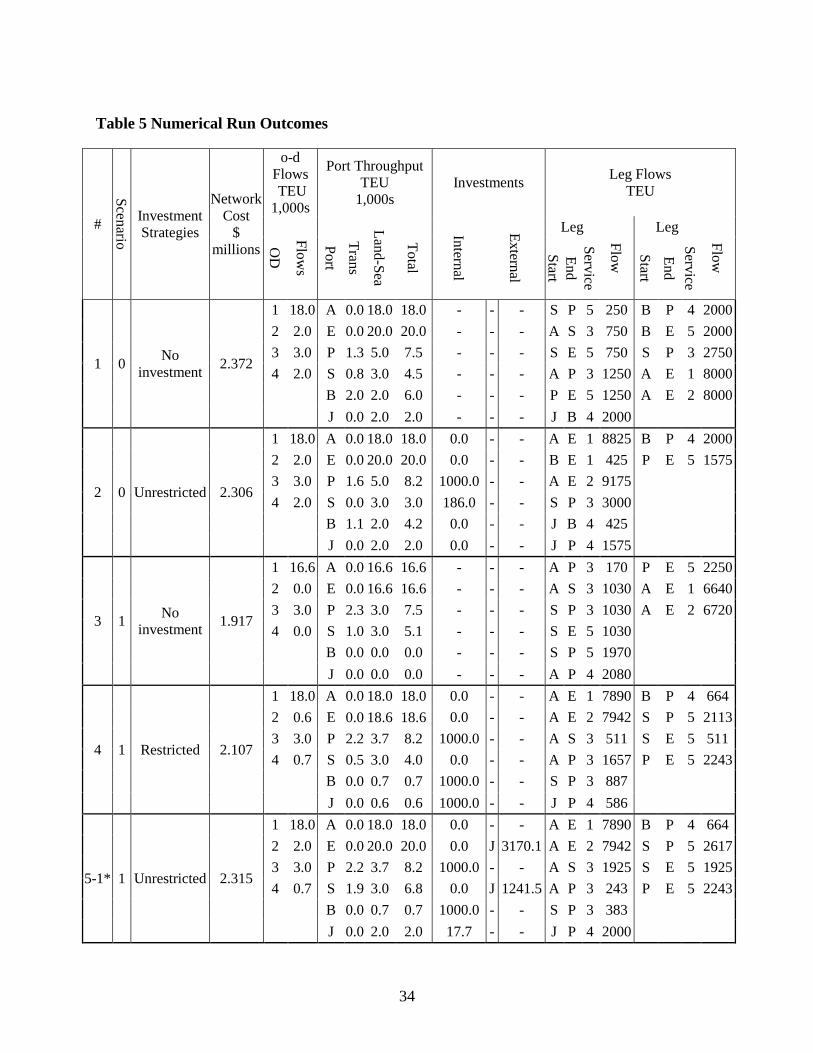
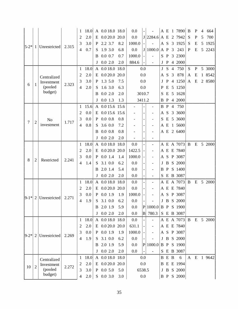
The outcomes of the numerical runs are provided in Table 5. For this example problem, the
MPEC has 389 continuous variables, 191 binary variables and 585 constraints. With appropriate
settings, the solution time for each MPEC ranged from a couple of seconds to one minute. The
scenario’s characteristics do not impact solution times. Thus, solutions were obtained for the
ports over iterations required to achieve convergence in a few minutes. The number of binary
variables will have greatest impact for large problem instances, as for large networks
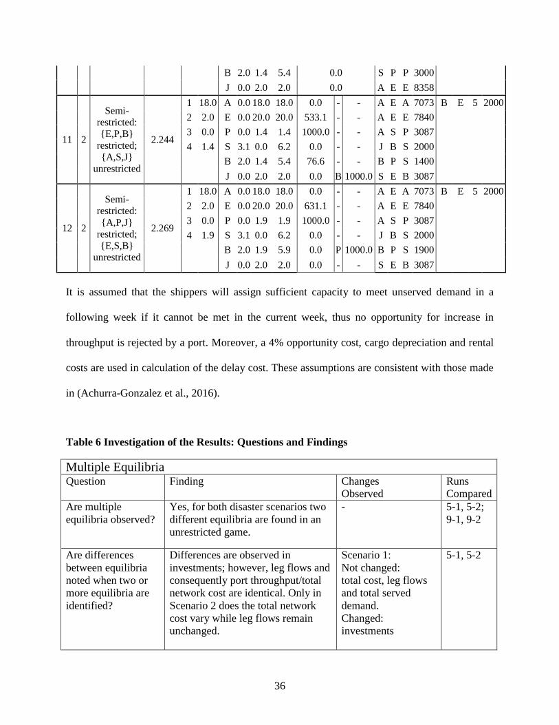
. These results were studied to investigate answers to a
number of questions. These questions and findings or observations and the runs from which the
findings are obtained are given in Table 6.
34
Table 5 Numerical Run Outcomes
#
Scen
ario
Investment
Strategies
Network
Cost
$
millions
o-d
Flows
TEU
1,000s
Port Throughput
TEU
1,000s
Investments Leg Flows
TEU
OD
Flo
ws
Po
rt
Tran
s
Lan
d-S
ea
To
tal
Intern
al
Ex
ternal
Leg
Flo
w
Leg
Flo
w
Start
En
d
Serv
ice
Start
En
d
Serv
ice
1 0 No
investment 2.372
1 18.0 A 0.0 18.0 18.0 - - - S P 5 250 B P 4 2000
2 2.0 E 0.0 20.0 20.0 - - - A S 3 750 B E 5 2000
3 3.0 P 1.3 5.0 7.5 - - - S E 5 750 S P 3 2750
4 2.0 S 0.8 3.0 4.5 - - - A P 3 1250 A E 1 8000
B 2.0 2.0 6.0 - - - P E 5 1250 A E 2 8000
J 0.0 2.0 2.0 - - - J B 4 2000
2 0 Unrestricted 2.306
1 18.0 A 0.0 18.0 18.0 0.0 - - A E 1 8825 B P 4 2000
2 2.0 E 0.0 20.0 20.0 0.0 - - B E 1 425 P E 5 1575
3 3.0 P 1.6 5.0 8.2 1000.0 - - A E 2 9175
4 2.0 S 0.0 3.0 3.0 186.0 - - S P 3 3000
B 1.1 2.0 4.2 0.0 - - J B 4 425
J 0.0 2.0 2.0 0.0 - - J P 4 1575
3 1 No
investment 1.917
1 16.6 A 0.0 16.6 16.6 - - - A P 3 170 P E 5 2250
2 0.0 E 0.0 16.6 16.6 - - - A S 3 1030 A E 1 6640
3 3.0 P 2.3 3.0 7.5 - - - S P 3 1030 A E 2 6720
4 0.0 S 1.0 3.0 5.1 - - - S E 5 1030
B 0.0 0.0 0.0 - - - S P 5 1970
J 0.0 0.0 0.0 - - - A P 4 2080
4 1 Restricted 2.107
1 18.0 A 0.0 18.0 18.0 0.0 - - A E 1 7890 B P 4 664
2 0.6 E 0.0 18.6 18.6 0.0 - - A E 2 7942 S P 5 2113
3 3.0 P 2.2 3.7 8.2 1000.0 - - A S 3 511 S E 5 511
4 0.7 S 0.5 3.0 4.0 0.0 - - A P 3 1657 P E 5 2243
B 0.0 0.7 0.7 1000.0 - - S P 3 887
J 0.0 0.6 0.6 1000.0 - - J P 4 586
5-1* 1 Unrestricted 2.315
1 18.0 A 0.0 18.0 18.0 0.0 - - A E 1 7890 B P 4 664
2 2.0 E 0.0 20.0 20.0 0.0 J 3170.1 A E 2 7942 S P 5 2617
3 3.0 P 2.2 3.7 8.2 1000.0 - - A S 3 1925 S E 5 1925
4 0.7 S 1.9 3.0 6.8 0.0 J 1241.5 A P 3 243 P E 5 2243
B 0.0 0.7 0.7 1000.0 - - S P 3 383
J 0.0 2.0 2.0 17.7 - - J P 4 2000
35
5-2* 1 Unrestricted 2.315
1 18.0 A 0.0 18.0 18.0 0.0 - - A E 1 7890 B P 4 664
2 2.0 E 0.0 20.0 20.0 0.0 J 2284.6 A E 2 7942 S P 5 700
3 3.0 P 2.2 3.7 8.2 1000.0 - - A S 3 1925 S E 5 1925
4 0.7 S 1.9 3.0 6.8 0.0 J 1000.0 A P 3 243 P E 5 2243
B 0.0 0.7 0.7 1000.0 - - S P 3 2300
J 0.0 2.0 2.0 884.6 - - J P 4 2000
6 1
Centralized
Investment
(pooled
budget)
2.323
1 18.0 A 0.0 18.0 18.0 0.0 J S 4 750 S P 5 3000
2 2.0 E 0.0 20.0 20.0 0.0 A S 3 878 A E 1 8542
3 3.0 P 1.3 5.0 7.5 0.0 J P 4 1250 A E 2 8580
4 2.0 S 1.6 3.0 6.3 0.0 P E 5 1250
B 0.0 2.0 2.0 3010.7 S E 5 1628
J 0.0 1.3 1.3 3411.2 B P 4 2000
7 2 No
investment 1.717
1 15.6 A 0.0 15.6 15.6 - - - B P 4 750
2 0.0 E 0.0 15.6 15.6 - - - A S 3 3600
3 0.0 P 0.0 0.8 0.8 - - - S E 5 3600
4 0.8 S 3.6 0.0 7.2 - - - A E 1 5600
B 0.0 0.8 0.8 - - - A E 2 6400
J 0.0 2.0 2.0 - - -
8 2 Restricted 2.241
1 18.0 A 0.0 18.0 18.0 0.0 - - A E A 7073 B E 5 2000
2 2.0 E 0.0 20.0 20.0 1422.5 - - A E E 7840
3 0.0 P 0.0 1.4 1.4 1000.0 - - A S P 3087
4 1.4 S 3.1 0.0 6.2 0.0 - - J B S 2000
B 2.0 1.4 5.4 0.0 - - B P S 1400
J 0.0 2.0 2.0 0.0 - - S E B 3087
9-1* 2 Unrestricted 2.271
1 18.0 A 0.0 18.0 18.0 0.0 - - A E A 7073 B E 5 2000
2 2.0 E 0.0 20.0 20.0 0.0 - - A E E 7840
3 0.0 P 0.0 1.9 1.9 1000.0 - - A S P 3087
4 1.9 S 3.1 0.0 6.2 0.0 - - J B S 2000
B 2.0 1.9 5.9 0.0 P 1000.0 B P S 1900
J 0.0 2.0 2.0 0.0 B 780.3 S E B 3087
9-2* 2 Unrestricted 2.269
1 18.0 A 0.0 18.0 18.0 0.0 - - A E A 7073 B E 5 2000
2 2.0 E 0.0 20.0 20.0 631.1 - - A E E 7840
3 0.0 P 0.0 1.9 1.9 1000.0 - - A S P 3087
4 1.9 S 3.1 0.0 6.2 0.0 - - J B S 2000
B 2.0 1.9 5.9 0.0 P 1000.0 B P S 1900
J 0.0 2.0 2.0 0.0 - - S E B 3087
10 2
Centralized
Investment
(pooled
budget)
2.272
1 18.0 A 0.0 18.0 18.0 0.0 B E B 6 A E 1 9642
2 2.0 E 0.0 20.0 20.0 0.0 B E E 1994
3 3.0 P 0.0 5.0 5.0 6538.5 J B S 2000
4 2.0 S 0.0 3.0 3.0 0.0 B P S 2000
36
B 2.0 1.4 5.4 0.0 S P P 3000
J 0.0 2.0 2.0 0.0 A E E 8358
11 2
Semi-
restricted:
{E,P,B}
restricted;
{A,S,J}
unrestricted
2.244
1 18.0 A 0.0 18.0 18.0 0.0 - - A E A 7073 B E 5 2000
2 2.0 E 0.0 20.0 20.0 533.1 - - A E E 7840
3 0.0 P 0.0 1.4 1.4 1000.0 - - A S P 3087
4 1.4 S 3.1 0.0 6.2 0.0 - - J B S 2000
B 2.0 1.4 5.4 76.6 - - B P S 1400
J 0.0 2.0 2.0 0.0 B 1000.0 S E B 3087
12 2
Semi-
restricted:
{A,P,J}
restricted;
{E,S,B}
unrestricted
2.269
1 18.0 A 0.0 18.0 18.0 0.0 - - A E A 7073 B E 5 2000
2 2.0 E 0.0 20.0 20.0 631.1 - - A E E 7840
3 0.0 P 0.0 1.9 1.9 1000.0 - - A S P 3087
4 1.9 S 3.1 0.0 6.2 0.0 - - J B S 2000
B 2.0 1.9 5.9 0.0 P 1000.0 B P S 1900
J 0.0 2.0 2.0 0.0 - - S E B 3087
It is assumed that the shippers will assign sufficient capacity to meet unserved demand in a
following week if it cannot be met in the current week, thus no opportunity for increase in
throughput is rejected by a port. Moreover, a 4% opportunity cost, cargo depreciation and rental
costs are used in calculation of the delay cost. These assumptions are consistent with those made
in (Achurra-Gonzalez et al., 2016).
Table 6 Investigation of the Results: Questions and Findings
Multiple Equilibria Question Finding Changes
Observed
Runs
Compared
Are multiple
equilibria observed?
Yes, for both disaster scenarios two
different equilibria are found in an
unrestricted game.
- 5-1, 5-2;
9-1, 9-2
Are differences
between equilibria
noted when two or
more equilibria are
identified?
Differences are observed in
investments; however, leg flows and
consequently port throughput/total
network cost are identical. Only in
Scenario 2 does the total network
cost vary while leg flows remain
unchanged.
Scenario 1:
Not changed:
total cost, leg flows
and total served
demand.
Changed:
investments
5-1, 5-2
37
Scenario 2:
Not changed:
leg flows and total
served demand.
Changed:
investments, total
shipping costs
9-1, 9-2
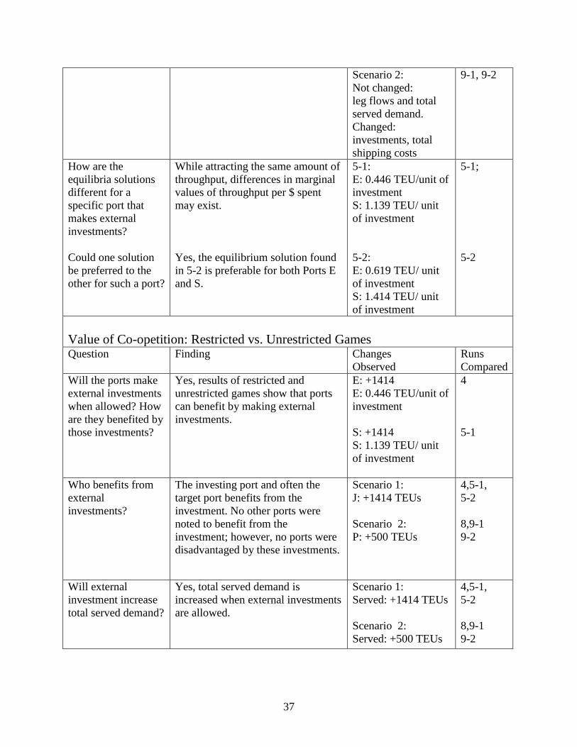
How are the
equilibria solutions
different for a
specific port that
makes external
investments?
Could one solution
be preferred to the
other for such a port?
While attracting the same amount of
throughput, differences in marginal
values of throughput per $ spent
may exist.
Yes, the equilibrium solution found
in 5-2 is preferable for both Ports E
and S.
5-1:
E: 0.446 TEU/unit of
investment
S: 1.139 TEU/ unit
of investment
5-2:
E: 0.619 TEU/ unit
of investment
S: 1.414 TEU/ unit
of investment
5-1;
5-2
Value of Co-opetition: Restricted vs. Unrestricted Games
Question Finding Changes
Observed
Runs
Compared
Will the ports make
external investments
when allowed? How
are they benefited by
those investments?
Yes, results of restricted and
unrestricted games show that ports
can benefit by making external
investments.
E: +1414
E: 0.446 TEU/unit of
investment
S: +1414
S: 1.139 TEU/ unit
of investment
4
5-1
Who benefits from
external
investments?
The investing port and often the
target port benefits from the
investment. No other ports were
noted to benefit from the
investment; however, no ports were
disadvantaged by these investments.
Scenario 1:
J: +1414 TEUs
Scenario 2:
P: +500 TEUs
4,5-1,
5-2
8,9-1
9-2
Will external
investment increase
total served demand?
Yes, total served demand is
increased when external investments
are allowed.
Scenario 1:
Served: +1414 TEUs
Scenario 2:
Served: +500 TEUs
4,5-1,
5-2
8,9-1
9-2

38
Does the unrestricted
investment strategy
decrease total
network shipping
cost compared to
costs incurred with a
restricted strategy?*
Yes, for both scenarios the network
costs decrease when ports are
allowed to make external
investments.
Scenario 1:
5-1/5-2 vs. 4: -3.0%
Scenario 2:
9-1 vs. 8: -2.4%
9-2 vs. 8: -2.5%
4,5
9-1,8
9-2,8
Gains and Losses in Market Share in Disaster
Question Finding Changes
Observed
Runs
Compared
Does any port
benefit from a
disaster scenario
(without further
investment)?
Yes, Port S takes greater market
share in the aftermath of Scenario 1.
However, it is worth noting that this
port loses under Scenario 2.
Scenario 1:
S: +280 TEUs
Scenario 2:
S: -150 TEUs
1,3
1,7
Can internal-only
investments harm
any port in terms of
throughput?
Yes, Port S serves fewer units when
under the restricted investment
strategy, showing that the other
ports, through self-investment, can
outcompete Port S for market share.
Scenario 1:
S: -519 TEUs
Scenario 2:
S: -513 TEUs
3,4
7,8
Centralized Decision Making
Question Finding Changes
Observed
Runs
Compared
Does centralizing
investments increase
total throughput for
the port network?
Yes, a centralized approach leads to
greater total throughput under either
disaster scenarios. The results
indicate a reduction in total
transshipments, but an increase in
land-sea throughput.
Scenario 1:
Trans.:-1290 TEUs
Land-Sea:+1921
TEUs
Total:+632 TEUs
Scenario 2:
Trans.:-3087 TEUs
Land-Sea:+5600
TEUs
Total:+2513 TEUs
5-1,
5-2,6
9-1,
9-2,10
Who wins or loses
under a centralized
investment scheme?
Ports S and J lose under Scenario 1,
while Ports S and B lose under
Scenario 2. Port B wins under
Scenario 1, and Port P wins under
both scenarios.
Scenario 1:
S :-297 TEUs
J: -750 TEUs
P: +343 TEUs
B: +1336 TEUs
Scenario 2:
S: -87 TEUs
5,6
9,10

39
B: -500 TEUs
P: +3100 TEUs
How significant is
the gain to the
system of a
centralized
investment scheme
in helping the system
to recover from a
disaster event?
Considering scenario 1, an increase
in total served demand of 12.36%
and 5.64% compared with restricted
and unrestricted investment
approaches, respectively, and
27.29% compared with no
investment is noted.
Served:
6 vs. 3: +2749 TEUs
6 vs. 4: +1336 TEUs
6 vs. 5-1,5-2: +5360
TEUs
5,6
9,10
Does a centralized
investment scheme
reduce total network
shipping cost?*
Yes. Scenario 1:
6 vs. 1: -2.1%
6 vs 5-1,5-2: -10.2%
Scenario 2:
10 vs. 1: -4.2%
10 vs. 2: -1.5%
10 vs. 9-1: -21.6%
10 vs. 9-2: -21.6%
6,1
6,5
10,1
10,2
10,9-1
10,9-2
Benefits of Unreciprocated Investments
Finding Changes
Observed
Runs Compared
If some ports do not
consider external
investment, will
other ports still
invest in them?
Yes, Port B invests in Port P even
when Ports A, P and J do not
consider making external
investments. However, when Port B
restricts itself to an internal
investment strategy, Port J stops
making external investments in Port
B.
No change in Port B
external investments
J: -780.33 TEUs
12,9-1
11-2, 9-1
Do ports that invest
only internally gain
or lose?
They can lose, but did not gain.
When E, P and B only invest
internally, Ports B and P lose market
share. When A, P and J only invest
internally, no port experiences a
change in market share.
P: -400 TEUs
B: -400 TEUs
E: No change
P: No change
B: No change
E: No change
9,11
9,12

40
These experiments helped to gain insights into the potential benefits of a co-opetitive approach to
global port. The results indicate that while a port may gain throughput when no investments are
made under a particular scenario, they are not likely to gain under all scenarios. Moreover, the
total market served may be reduced in which case gains may exist in market share, but not
necessarily in throughput or revenue. Ports can themselves gain by helping to protect other ports
in the global supply chain. Gains can be achieved even when investments are not reciprocated.
Facilitating a co-opetitive environment supports greater overall throughput and reduces overall
network shipping costs as compared to using similar funds for only internal investments.
Benefits are obtained for both ports and shippers alike.
41
5.0 CONCLUSIONS AND DISCUSSION
This paper develops a formulation and solution technique for a co-opetitive, protective
investment problem arising in a maritime port network that serves a common liner shipping
market. This work adds to the rich body of literature in port and maritime resiliency by
conceptualizing multi-port investments and liner-shipping network response as a multi-leader,
common-follower game. As compared to non-cooperative approaches, in the presence of a
disaster event, the proposed co-opetitive approach was found to lead to increased served total
demand, significantly increased market share for many ports and improved services for shippers,
thus creating greater system-wide resiliency. As in any competitive environment, there are
winners and losers. This work shows that it is often beneficial to an individual port in terms of
market share to invest in another part of the maritime port network. This modeling framework
allows for: the simultaneous consideration of market interactions; disaster and investment
impacts; inter-port, service-level dependencies; cooperation; and competition. This structure
helps in providing a more realistic assessment compared to traditional centralized or independent
formulation schemes, and enables quantification of benefits of varying co-opetitive approaches
and effectiveness of chosen investments. It quantifies the losses due to myopic intra-port (as
opposed to inter-port) investments. A stochastic extension of the proposed EPEC aimed at
identifying investment strategies that simultaneously hedge against multiple potential hazard
scenarios is the subject of ongoing work by the authors.
As is common in equilibria modeling, more than one equilibrium may exist. These solutions may
not be equivalent or may better serve one stake-holder over another. An objective function can
42
be added to the EPEC formulation to guide the formulation toward a solution that best serves that
objective. Alternatively, multiple equilibria can be sought through multi-start techniques as
implemented herein to produce a set of equilibria solutions if more than one equilibrium exists
and a best compromise solution much like in multi-objective decision-making can be chosen.
The ports serve not only the liner shipping market, but local, regional and national businesses
and manufacturers who depend on both the raw or processed materials they supply as well as the
transport of finished goods to retailers across the world. Port reliability also concerns end-
customers who are affected by increases in the price of goods.
Solution of the EPEC formulation involved several computational challenges. Inconsistencies
between solutions of the equivalent KKT conditions of the common liner shipping problem were
sometimes noted. Use of very small integrality gaps in solution of the MPEC MIPs was required
to ensure numerical stability and consistency across players. The solution technique was found to
be sensitive to the setting of M. This setting affected both the ability to obtain a solution and the
speed at which a solution was found. M is introduced through linearization of the
complementarity constraints associated with the KKT conditions of the lower-level problem
through a disjunctive constraints approach. An alternative method might be to apply Schur’s
decomposition (Horn & Johnson 1985) using Special Ordered Sets of Type 1 (SOS1) variables
(Siddiqui & Gabriel 2013).

43

44
6.0 REFERENCES
Achurra-Gonzalez, P.E. et al., 2016. Modelling the impact of liner shipping network
perturbations on container cargo routing: Southeast Asia to Europe application. Accident
Analysis & Prevention.
Angeloudis, P. et al., 2007. Security and reliability of the liner container-shipping network:
analysis of robustness using a complex network framework. Bichou, K, Bell, MGH and
Evans, A.
Asgari, N., Farahani, R.Z. & Goh, M., 2013. Network design approach for hub ports-shipping
companies competition and cooperation. Transportation Research Part A: Policy and
Practice, 48, pp.1–18.
Bakshi, N. & Kleindorfer, P., 2009. Co‐opetition and investment for supply‐chain resilience.
Production and Operations Management, 18(6), pp.583–603.
Becker, A. et al., 2012. Climate change impacts on international seaports: knowledge,
perceptions, and planning efforts among port administrators. Climatic Change, 110(1–2),
pp.5–29. Available at: http://link.springer.com/10.1007/s10584-011-0043-7 [Accessed
December 7, 2016].
Bell, M.G.H. et al., 2013. A cost-based maritime container assignment model. Transportation
Research Part B: Methodological, 58, pp.58–70.
Brooks, M.R., 2004. The governance structure of ports. Review of Network Economics, 3(2).
Chang, S.E., 2000. Disasters and transport systems: loss, recovery and competition at the Port of
Kobe after the 1995 earthquake. Journal of Transport Geography, 8(1), pp.53–65.
Available at: http://www.sciencedirect.com/science/article/pii/S096669239900023X
[Accessed May 15, 2017].
Chen, H.-C. & Liu, S.-M., 2016. Should ports expand their facilities under congestion and
uncertainty? Transportation Research Part B: Methodological, 85, pp.109–131. Available
at: http://www.sciencedirect.com/science/article/pii/S0191261516000035 [Accessed
October 11, 2017].
Chen, L. & Miller-Hooks, E., 2012. Resilience: an indicator of recovery capability in intermodal
freight transport. Transportation Science, 46(1), pp.109–123.
Do, T.M.H. et al., 2015. Application of Game Theory and Uncertainty Theory in Port
Competition between Hong Kong Port and Shenzhen Port. International Journal of e-
Navigation and Maritime Economy, 2, pp.12–23.
Fortuny-Amat, J. & McCarl, B., 1981. A representation and economic interpretation of a two-
level programming problem. Journal of the operational Research Society, pp.783–792.
Gabriel, S.A. et al., 2013. Complementarity Modeling in Energy Markets, New York, NY:
Springer New York. Available at: http://link.springer.com/10.1007/978-1-4419-6123-5
[Accessed January 27, 2017].
Hishamuddin, H., Sarker, R.A. & Essam, D., 2013. A recovery model for a two-echelon serial
supply chain with consideration of transportation disruption. Computers & Industrial
Engineering, 64(2), pp.552–561.
Ho, W. et al., 2015. Supply chain risk management: a literature review. International Journal of
45
Production Research, 53(16), pp.5031–5069.
Horn, R.A. & Johnson, C.R., 1985. Matrix Analysis Cambridge University Press. New York.
Ishii, M. et al., 2013. A game theoretical analysis of port competition. Transportation Research
Part E: Logistics and Transportation Review, 49(1), pp.92–106.
Lee, H., Boile, M., et al., 2014. A freight network planning model in oligopolistic shipping
markets. Cluster Computing, 17(3), pp.835–847. Available at:
http://link.springer.com/10.1007/s10586-013-0314-3 [Accessed October 22, 2017].
Lee, H., Song, Y., et al., 2014. Bi-level optimization programming for the shipper-carrier
network problem. Cluster Computing, 17(3), pp.805–816. Available at:
http://link.springer.com/10.1007/s10586-013-0311-6 [Accessed October 22, 2017].
Lee, H. & Choo, S., 2016. Optimal decision making process of transportation service providers
in maritime freight networks. KSCE Journal of Civil Engineering, 20(2), pp.922–932.
Available at: http://link.springer.com/10.1007/s12205-015-0116-7 [Accessed October 22,
2017].
Loh, H.S. & Van Thai, V., 2014. Managing Port-Related Supply Chain Disruptions: A
Conceptual Paper. The Asian Journal of Shipping and Logistics, 30(1), pp.97–116.
Mansouri, M., Sauser, B. & Boardman, J., 2009. Applications of systems thinking for resilience
study in Maritime Transportation System of Systems. In 2009 3rd Annual IEEE Systems
Conference. IEEE, pp. 211–217. Available at: http://ieeexplore.ieee.org/document/4815800/
[Accessed December 9, 2016].
Nair, R., Avetisyan, H. & Miller-Hooks, E., 2010. Resilience Framework for Ports and Other
Intermodal Components. Transportation Research Record: Journal of the Transportation
Research Board, 2166, pp.54–65. Available at:
http://trrjournalonline.trb.org/doi/10.3141/2166-07 [Accessed January 5, 2017].
Nalebuff, B., Brandenburger, A. & Maulana, A., 1996. Co-opetition, HarperCollinsBusiness
London.
Omer, M. et al., 2012. A framework for assessing resiliency of maritime transportation systems.
Maritime Policy & Management, 39(7), pp.685–703. Available at:
http://www.tandfonline.com/doi/abs/10.1080/03088839.2012.689878 [Accessed December
8, 2016].
Peng, Y. et al., 2016. A stochastic seaport network retrofit management problem considering
shipping routing design. Ocean & Coastal Management, 119, pp.169–176.
Python, G.C. & Wakeman, T.H., 2016. Collaboration of Port Members for Supply Chain
Resilience. In Ports 2016. Reston, VA: American Society of Civil Engineers, pp. 371–380.
Available at: http://ascelibrary.org/doi/10.1061/9780784479902.038 [Accessed December
7, 2016].
Reilly, A.C., Samuel, A. & Guikema, S.D., 2015. “Gaming the System”: Decision Making by
Interdependent Critical Infrastructure. Decision Analysis, 12(4), pp.155–172. Available at:
http://pubsonline.informs.org/doi/10.1287/deca.2015.0318 [Accessed December 13, 2016].
Rienkhemaniyom, K. & Ravindran, A.R., 2014. Global Supply Chain Network Design
Incorporating Disruption Risk. International Journal of Business Analytics (IJBAN), 1(3),
pp.37–62.
Rose, A. & Wei, D., 2013. ESTIMATING THE ECONOMIC CONSEQUENCES OF A PORT
SHUTDOWN: THE SPECIAL ROLE OF RESILIENCE. Economic Systems Research,
25(2), pp.212–232. Available at:
http://www.tandfonline.com/doi/abs/10.1080/09535314.2012.731379 [Accessed December
46
7, 2016].
Shafieezadeh, A. & Ivey Burden, L., 2014. Scenario-based resilience assessment framework for
critical infrastructure systems: Case study for seismic resilience of seaports. Reliability
Engineering & System Safety, 132, pp.207–219.
Shaw, D.R., Grainger, A. & Achuthan, K., 2016. Multi-level port resilience planning in the UK:
How can information sharing be made easier? Technological Forecasting and Social
Change.
Siddiqui, S. & Gabriel, S.A., 2013. An SOS1-based approach for solving MPECs with a natural
gas market application. Networks and Spatial Economics, 13(2), pp.205–227.
Sokolov, B. et al., 2016. Structural quantification of the ripple effect in the supply chain.
International Journal of Production Research, 54(1), pp.152–169. Available at:
http://www.tandfonline.com/doi/full/10.1080/00207543.2015.1055347 [Accessed January
18, 2017].
Song, D.-P. et al., 2016. Modeling port competition from a transport chain perspective.
Transportation Research Part E: Logistics and Transportation Review, 87, pp.75–96.
Available at: http://linkinghub.elsevier.com/retrieve/pii/S1366554515300478 [Accessed
October 11, 2017].
Song, D.-W. & Panayides, P.M., 2012. Maritime logistics: contemporary issues, Emerald Group
Publishing.
Song, L. et al., 2016. A game-theoretical approach for modeling competitions in a maritime
supply chain. Maritime Policy & Management, 43(8), pp.976–991. Available at:
https://www.tandfonline.com/doi/full/10.1080/03088839.2016.1231427 [Accessed October
11, 2017].
Tang, C., 2006. Robust strategies for mitigating supply chain disruptions. International Journal
of Logistics, 9(1), pp.33–45. Available at:
http://www.tandfonline.com/doi/abs/10.1080/13675560500405584 [Accessed May 15,
2017].
Tran, N.K. & Haasis, H.-D., 2015. Literature survey of network optimization in container liner
shipping. Flexible Services and Manufacturing Journal, 27(2–3), pp.139–179. Available at:
http://link.springer.com/10.1007/s10696-013-9179-2 [Accessed February 2, 2017].
Wu, T., Blackhurst, J. & O’grady, P., 2007. Methodology for supply chain disruption analysis.
International Journal of Production Research, 45(7), pp.1665–1682. Available at:
http://www.tandfonline.com/doi/abs/10.1080/00207540500362138 [Accessed January 18,
2017].
Yang, Z. et al., Modelling risk based cost analysis of port adaptation measures to climate change.
Zhang, T., Zhao, Q. & Wu, W., 2009. Bi-level programming model of container port game in the
container transport supernetwork. Journal of Applied Mathematics and Computing, 31(1–2),
pp.13–32. Available at: http://link.springer.com/10.1007/s12190-008-0188-3 [Accessed
October 22, 2017].
Zhuang, W., Luo, M. & Fu, X., 2014. A game theory analysis of port specialization—
implications to the Chinese port industry. Maritime Policy & Management, 41(3), pp.268–
287. Available at: http://www.tandfonline.com/doi/abs/10.1080/03088839.2013.839517
[Accessed October 11, 2017].