Embed Size (px)
Citation preview
W O R K S H O P
Prospectivity mapping in GIS: integrate geochemistry data with
geophysics and geology

Prospectivity mapping in GIS: integrate geochemistry data with geophysics
and geology
Workshop, 21 August 2011
25th International Applied Geochemistry Symposium 201122-26 August 2011 Rovaniemi, Finland
Vesa Nykänen
Publisher: Vuorimiesyhdistys - Finnish Association of Mining and Metallurgical
Engineers, Serie B, Nro B92-5, Rovaniemi 2011

Nykänen, V. 2011. Prospectivity mapping in GIS: integrate geochemistry data with geophysics and geology. Workshop in the 25th International Applied Geochemistry Symposium 2011 22-26 August 2011 Rovani-emi, Finland. Vuorimiesyhdistys, B92-5, 88 pages.
Layout:Cover – Irma Varrio
ISBN 978-952-9618-72-9 (Printed) ISBN 978-952-9618-73-6 (Pdf)ISSN 0783-1331
© Vuorimiesyhdistys
This volume is available from:Vuorimiesyhdistys ry.Kaskilaaksontie 3 D 10802360 ESPOO
Electronic version:http://www.iags2011.fi or http://www.vuorimiesyhdistys.fi/julkaisut.php
Printed in:Painatuskeskus Finland Oy, Rovaniemi

Prospectivity mapping in GIS: integrate geochemistry data with geophysics and geology
Vesa NykänenGeological Survey of FinlandP.O. Box 77, FIN-96101 Rovaniemi, FinlandEmail: [email protected]
Abstract
Prospectivity mapping is used to define areas favourable for mineral exploration. It can be applied in various scales from global to local scale exploration targeting. Geographical information systems (GIS) provide a flexible and powerful platform to apply spatial data analysis techniques as a tool for prospectivity mapping by in-tegrating geochemical, geophyscical and geological data. These techniques include e.g. weights of evidence, logistic regression, fuzzy logic and neural networks. Definition of the exploration model can be based on a genetic ore deposit model or a mineral system model. This gives the framework for the data used for creating a predictive prospectivity analysis for mineral exploration targeting. Es-sential part of the procedure is the pre-processing of the raw data into meaningful map patterns for the given task. These pre-processing techniques include data in-terpolation, classification, clustering, rescaling, filtering, image processing, raster calculation etc. A common expression for describing these methods in GIS platform is geoprocessing. After creating the map patterns indicating the vectors towards a mineral deposit type we can apply various data integration techniques in GIS to create a single prospectivity map delineating positive areas for mineral exploration. Application of these techniques using ArcGIS software and add-on applications will be discussed and demonstrated during this one day workshop. The examples pre-sented in this workshop give insights into the use of the techniques for exploration of orogenic gold, IOCG and magmatic Ni-Cu deposits.

6
Workshop Program Sunday, 21 August 2011, Hotel Santa Claus, Rovaniemi
8.30-9.00 Registration
9.00-10.15 Introduction and case histories • Aim of the workshop • Orogenic Au prospectivity • IOCG prospectivity • Ni prospectivity
10.15-10.30 Coffee/tea
10.30-12 Lab 1-3: Geoprosessing tools: ArcToolbox ja SDM Toolbox • Introduction to GIS • Demo 1 • Spatial analysis (buffers, proximity, density, interpolation…) • Demo 2 • Demo 3 12-13 Lunch
13-14 Lab 4-6: Weights of evidence • Training sites, calculating weights, creating a prospectivity map • Demo 4 • Demo 5 • Demo 6
14-15 Lab 7: Fuzzy logic • Fuzzy set theory • Fuzzification functions • Fuzzy membership • Demo 7
15-15.15 Coffee/tea
15.15-16 Lab 8: Neural networks • The Principles of Neural Networks in Prospectivity Mapping • Demo 8


1
Prospectivity mapping in GIS:
integrate geochemistry data with geophysics and geology
Presentation includes slides modified from
Warick Brown Graham Bonham-Carter
Gary RainesStephen Gardoll
David Groves
Juhani Ojala
Vesa NykänenVesa Nykänen
Outline9-10.15 Introduction and case histories
• Aim of the workshop• Orogenic Au prospectivity
• IOCG prospectivity
• Ni prospectivity
10.15-10.30 Coffee/tea
10.30-12 Lab 1-3: Geoprosessing tools: ArcToolbox ja SDM Toolbox
• Introduction to GIS• Demo 1
• Spatial analysis (buffers, proximity, density, interpolation…)
• Demo 2• Demo 3
12-13 Lunch
Outline
13-14 Lab 4-6: Weights of evidence• Training sites, calculating weights, creating a prospectivity map
• Demo 4
• Demo 5• Demo 6
14-15 Lab 7: Fuzzy logic• Fuzzy set theory
• Fuzzification functions
• Fuzzy membership• Demo 7
15-15.15 Coffee/tea
15.15-16 Lab 8: Neural networks
• The Principles of Neural Networks in Prospectivity Mapping
• Demo 8
2
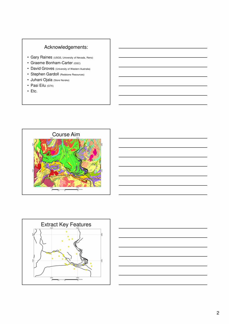
Acknowledgements:
• Gary Raines (USGS, University of Nevada, Reno)
• Graeme Bonham-Carter (GSC)
• David Groves (University of Western Australia)
• Stephen Gardoll (Redstone Resources)
• Juhani Ojala (Store Norske)
• Pasi Eilu (GTK)
• Etc.
Course Aim
Extract Key Features
3
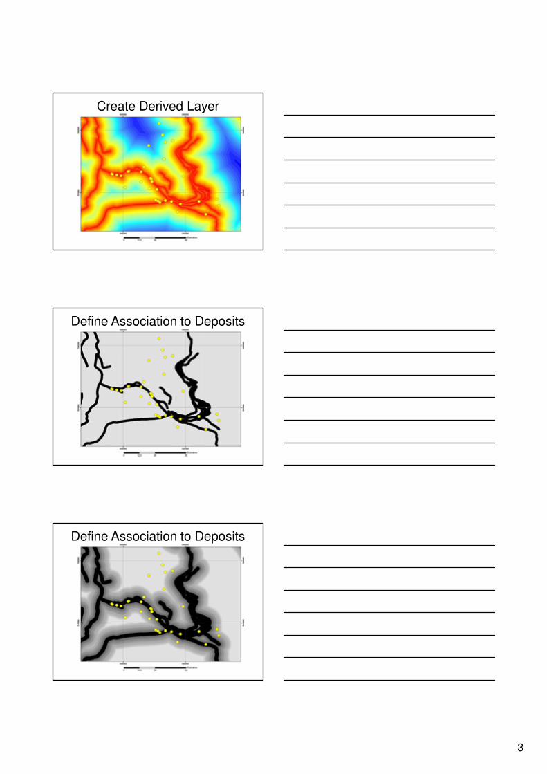
Create Derived Layer
Define Association to Deposits
Define Association to Deposits

4
Define Association to Deposits for Several Layers
Combine all Association into Prospectivity Map
Spatial modelling
• Spatial model is a generalization of real world
• Geologic map is a model
• Spatial model:
– Classifies geographic areas based on certain criteria (attributes)
– Makes predictions of phenomena
– Can be used in decicion making process to help undestanding real world systems
5
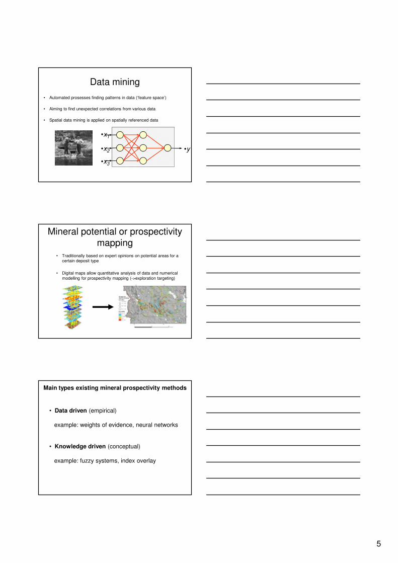
Data mining
• Automated prosesses finding patterns in data (‘feature space’)
• Aiming to find unexpected correlations from various data
• Spatial data mining is applied on spatially referenced data
•y
•x1
•x3
•x2
Mineral potential or prospectivity
mapping• Traditionally based on expert opinions on potential areas for a
certain deposit type
• Digital maps allow quantitative analysis of data and numerical
modelling for prospectivity mapping (->exploration targeting)
Main types existing mineral prospectivity methods
• Data driven (empirical)
example: weights of evidence, neural networks
• Knowledge driven (conceptual)
example: fuzzy systems, index overlay
6
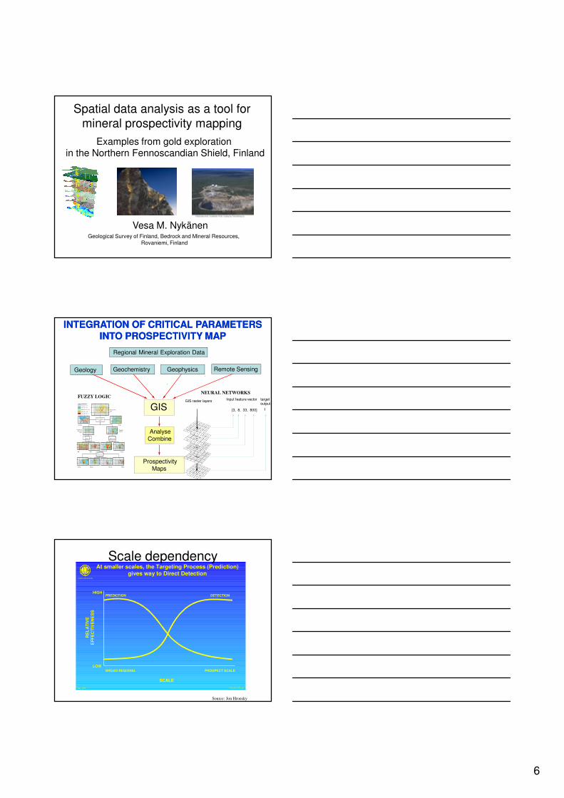
Spatial data analysis as a tool for
mineral prospectivity mapping
Vesa M. Nykänen
Examples from gold exploration in the Northern Fennoscandian Shield, Finland
Geological Survey of Finland, Bedrock and Mineral Resources,
Rovaniemi, Finland
ground acquisition target selectionProspectivity
Maps
INTEGRATION OF CRITICAL PARAMETERS INTEGRATION OF CRITICAL PARAMETERS INTO PROSPECTIVITY MAPINTO PROSPECTIVITY MAP
Regional Mineral Exploration Data
GIS
??Analyse
Combine
Remote SensingGeophysicsGeochemistryGeology
GIS raster layers target output
1
Input feature vector
[3, 8, 33, 800]
FUZZY LOGICNEURAL NETWORKS
((
(
((
(
((((
(
((
(
((
((
(
(
((
(
(
(
(((((((((
(((
(
(
(
(
(
(
((
(
((((
(
(
(
(
((
((
(
(
( (
(
(
(
(((((((((
(((
(
(
(
(
(
(
((
(
((((
(
(
(
(
((
((
(
(
( (
(
(
(
(((((((((
(((
(
(
(
(
(
(
((
(
((((
(
(
(
(
((
(
((
(
( (
(
(
(
(((((((((
(((
(
(
(
Till Fe
(
(
(
((
(
((((
(
(
(
(
((
((
(
(
((
(
(
(
(((((((((
(((
(
(
(
Till As
((
(
((
(
((((
(
(
(
(
((
(
((
(
((
(
(
(
(((((((((
(((
(
(
(
Till Te
(
(
(
((
(
((((
(
(
(
(
((
(
((
(
((
(
(
(
(((((((((
(((
(
(
(
Till Ni
(
(
(
((
(
((((
(
(
(
(
((
(
((
(
( (
(
(
(
(((((((((
(((
(
(
(
AM
(
(
(
((
(
((((
(
(
(
(
((
((
(
(
((
(
(
(
(((((((((
(((
(
(
(
EM
(
(
(
((
(
((((
(
(
(
(
((
(
((
(
( (
(
(
(
(((((((((
(((
(
(
(
Till Cu
(
(
(
((
(
((((
(
(
(
(
((
(((
(
( (
(
(
(
(((((((((
(((
(
(
(
Gravity
(
(
(
((
(
((((
(
(
(
(
((
((
(
(
((
(
(
(
(((((((((
(((
(
(
(
Till Au
(
(
(
((
(
((((
(
(
(
(
((
((
(
(
((
(
(
(
(((((((((
(((
(
(
(
Fuzzy Gammaγ=0.90
Fuzzy AndFuzzy And
Fuzzy Or
Fuzzy membership
Very low ( 0 - 0.2)
Low (0.21 - 0.4)
Moderate (0.41 - 0.6)
High (0.61 - 0.8)
Very high (0.81 - 1)
Conductive
alteration
zones
Sulphide
sources
Prospectivity
map
LOWBROAD REGIONAL
PREDICTION
At smaller scales, the Targeting Process (Prediction)gives way to Direct Detection
EXPLORATION
May 1999 From Bel-574.cdr
HIGH
PROSPECT SCALE
SCALE
RE
LA
TIV
EE
FF
EC
TIV
EN
ES
S
DETECTION
Source: Jon Hronsky
Scale dependency
7
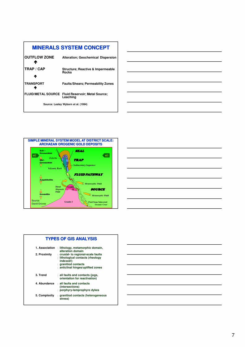
MINERALS SYSTEM CONCEPTMINERALS SYSTEM CONCEPT
OUTFLOW ZONE Alteration; Geochemical Dispersion
����
TRAP / CAP Structure; Reactive & Impermeable Rocks
����
TRANSPORT Faults/Shears; Permeability Zones����
FLUID/METAL SOURCE Fluid Reservoir; Metal Source; Leaching
Source: Lesley Wyborn et al. (1994)
SIMPLE MINERAL SYSTEM MODEL AT DISTRICT SCALE: SIMPLE MINERAL SYSTEM MODEL AT DISTRICT SCALE: ARCHAEAN OROGENIC GOLD DEPOSITSARCHAEAN OROGENIC GOLD DEPOSITS
Distal
Magmatic
Fluid
Fluid from Subcreted
Oceanic Crust
Metamorphic Fluid
Metamorphic Fluid
SOURCESOURCESOURCESOURCE
FLUID PATHWAYFLUID PATHWAYFLUID PATHWAYFLUID PATHWAY
TRAPTRAPTRAPTRAP
SEALSEALSEALSEAL
Granulite
Amphibolite
Mid -
Greenschist
Sub –
Greenschist
σ1σ1
Volcanic Rock
Dolerite
Sedimentary Sequence
Granite I
Granite
II
Source:
David Groves
TYPES OF GIS ANALYSISTYPES OF GIS ANALYSIS
1. Association
: lithology, metamorphic domain, alteration domain
2. Proximity
: crustal- to regional-scale faults : lithological contacts (rheology
indexed!) : granitiod contacts : anticlinal hinges/uplifted zones
3. Trend : all faults and contacts (jogs, orientation for reactivation)
4. Abundance : all faults and contacts (intersections)
: porphyry-lamprophyre dykes
5. Complexity : granitiod contacts (heterogeneous stress)

8
•I Empirical (data driven) approach
•Suitable for mature ’brown fields’ exploration terrains with abundant data available
•II Conceptual (knowledge driven) approach
•Suitable for ’green fields’ exploration terrains with limited number of deposits available for statistical assessment
Methods of spatial data analysis used for prospectivity mapping
•I Empirical (data driven) approach
•Known mineral occurrences as ‘training points’ are used for examining spatial relationships between known occurrences and particular geological, geochemical and geophysical key features
•Identified relationships are quantified and integrated into a single prospectivity map
•II Conceptual (knowledge driven) approach
•Re-formulation of knowledge about deposit formation into mappable criteria (i.e. threshold values in geochemistry and geophysics etc., certain structures or formations in the geological maps…)
•Areas that fulfill the majority of these criteria are highlighted as being the most prospective
•Methods of spatial data analysis used for prospectivity mapping
•I Empirical (data driven) approach
•Neural networks (RBFLN, PNN etc.)
•Weights of evidence, logistic regression
•II Conceptual (knowledge driven) approach
•Boolean logic
•Index overlay (binary or multi-class maps)
•Evidential belief function
•Dempster-Shafer model
•Decision tree approach
•Fuzzy logic
•Expert Weights of Evidence
•Methods of spatial data analysis used for prospectivity mapping
9
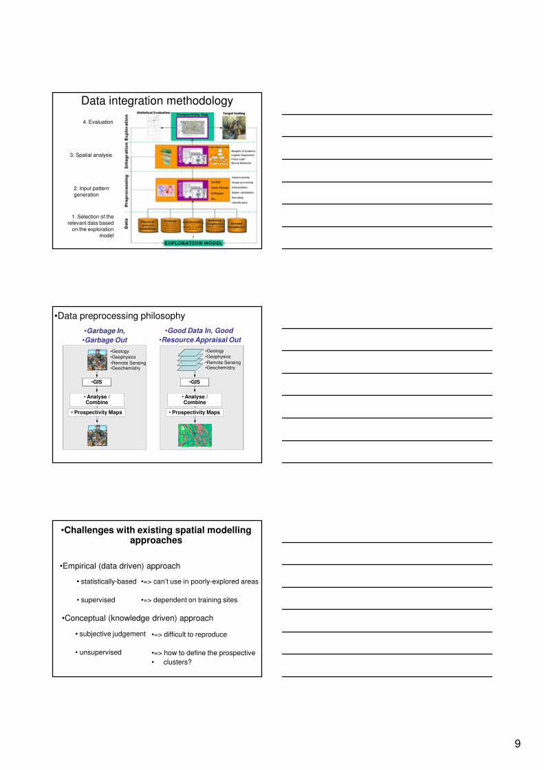
1. Selection of the
relevant data basedon the exploration
model
2. Input pattern
generation
3. Spatial analysis
4. Evaluation
Data integration methodology
•Data preprocessing philosophy
•Remote Sensing
•Geophysics
•Geochemistry
•Geology
•Garbage In,
•Garbage Out
• Prospectivity Maps
•GIS
• Analyse / Combine
• Prospectivity Maps
•GIS
• Analyse / Combine
•Good Data In, Good
•Resource Appraisal Out
•Remote Sensing
•Geophysics
•Geochemistry
•Geology
•Challenges with existing spatial modelling approaches
•Empirical (data driven) approach
•Conceptual (knowledge driven) approach
•=> can’t use in poorly-explored areas
•=> dependent on training sites
•=> difficult to reproduce
•=> how to define the prospective
• clusters?
•• subjective judgement
• unsupervised
•• statistically-based
• supervised

10
Orogenic vs. other gold deposit stylesOrogenic vs. other gold deposit styles
Tectonic setting of orogenic goldTectonic setting of orogenic gold
Gravity Airborne geophysics•magnetics•electro-magnetics•gamma radiationBedrock geologyGeochemistry SoilSatellite imagesModellingDigital elevationmodel and basemapsDigital map data

11
Study area
•Study Area: ~20 000 km2
•Northern FennoscandianShield•Located 100 km north from Arctic Circle•Excellent infrastructure•Green field exploration•35 orogenic Au occurrences•prior probability 0.0009
Study Area:Study Area:Central LaplandCentral LaplandGreenstoneGreenstoneBeltBelt
Suurikuusikko24.3 Mt @ 4.6 ppm Aures. 120t Au (3.7 MOz)
Pahtavaara2 Mt @ 2.5 ppm Aures. 10t Auproduction 1996-2000: 4.6t Au
Saattopora0.68 Mt @ 3.6 ppm Auproduction 1988-1995: 6.3t Au
Exploration Model
• Early Proterozoic greenstone hosted orogenic Au deposits
• Symptoms:
– Alteration zones with low magnetic and low resistivity signature,
– large scale crustal structures represented by horizontal gradient highs of regional gravity
– Anomalies in till indicating presence of sulphides and Au
12
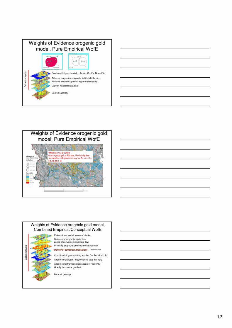
Weights of Evidence orogenic gold
model, Pure Empirical WofE
Bedrock geology
Gravity: horizontal gradient
Airborne electromagnetics: apparent resistivity
Airborne magnetics: magnetic field total intensity
Combined till geochemistry: As, Au, Cu, Fe, Ni and Te
Evid
en
ce
laye
rs
Weights of Evidence orogenic gold
model, Pure Empirical WofE
•High gravity gradient
•Aero-geophysics: AM low, Resistivity low•Anomalous till geochemistry for As, Au, Cu, Fe, Ni and Te
Weights of Evidence orogenic gold model, Combined Empirical/Conceptual WofE
Bedrock geology
Gravity: horizontal gradient
Airborne electromagnetics: apparent resistivity
Airborne magnetics: magnetic field total intensity
Combined till geochemistry: As, Au, Cu, Fe, Ni and Te
Density of contacts: Lithodiversity
Proximity to greenstone/sedimentary contact
Distance from granite midpoints:
zones of convergent/divergent flow
Palaeostress model: zones of dilation
Evid
en
ce
laye
rs
Poor correlation

13
Weights of Evidence orogenic gold model, Combined Empirical/Conceptual WofE
•High gravity gradient
•Aero-geophysics: AM low, Resistivity low•Anomalous till geochemistry for As, Au, Cu, Fe, Ni and Te
•Density of lithological contacts•Proximity to Sirkka Shear zone or divergent/convergent stress regimes
•Proximity to greenstone/sedimentary contacts•Paleostress modelling
Evidence Method Score W+ W- Contrast* Confidence
Gravity gradient CD 33 0.7757 -2.9342 3.7099 3.6544
Sirkka shear or zones of convergernt/divergent flow CD 30 0.7912 -1.6293 2.4205 4.5447
Apparent resistivity CA 19 1.5889 -0.6972 2.2860 6.5973
Proximity to sediment greenstone contacts CA 32 0.2710 -1.5683 1.8394 2.5227
Anomalous till geochemistry CD 27 0.5920 -1.0019 1.5939 3.7547
Aeromagnetic lows CA 9 1.3483 -0.2363 1.5846 4.0601
Paleosterss modeling CD 3 1.4148 -0.0462 1.4610 1.9942
Density of lithological contacts CD 28 0.1455 -0.4898 0.6353 1.4109
Total no of training sites = 34
Total area = 18642 km2
Prior probability = 0.0018
CD = weights calculated by cumulative descending method (i.e. from highest to lowest class)
CA = weights calculated by cumulative ascending method (i.e. from lowest to highest class)
Score = number of training sites within the 'inside' pattern
Contrast = W+ - W-
Confidence = Contrast/Std(Contrast)
Weights of Evidence
Positive evidence
Negative evidence
Summary of the weights calculation. The evidence is sorted by contrast values in descending order, the ’best’ layer on the top.
Artificial neural networks
y
x1
x3
x2
Supervised:
RBFLN, PNN, Fuzzy NN
Unsupervised:
SOM
14
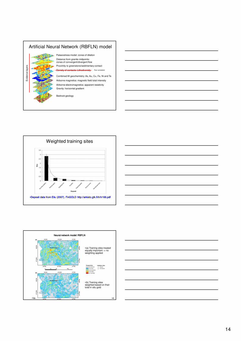
Artificial Neural Network (RBFLN) model
Bedrock geology
Gravity: horizontal gradient
Airborne electromagnetics: apparent resistivity
Airborne magnetics: magnetic field total intensity
Combined till geochemistry: As, Au, Cu, Fe, Ni and Te
Density of contacts: Lithodiversity
Proximity to greenstone/sedimentary contact
Distance from granite midpoints:
zones of convergent/divergent flow
Palaeostress model: zones of dilation
Evid
en
ce
laye
rs
Poor correlation
Weighted training sites
••Deposit data from Eilu (2007). FinGOLD http://arkisto.gtk.fi/tr/tr166.pdfDeposit data from Eilu (2007). FinGOLD http://arkisto.gtk.fi/tr/tr166.pdf
•42
•Vesa Nykänen, 23.3.2011
Neural network model: RBFLNNeural network model: RBFLN
•(a) Training sites treated equally important -> no weighting applied
•(b) Training sites weighted based on their total in situ gold

15
II Conceptual approach
• Step 1: Select data sets based on the exploration model
• Step 2: Assign fuzzy membership alues i.e. rescale all data into a common scale from 0 -> 1
(e.g. not favorable -> favorable)
• Step 3: Combine all the evidence data by using various fuzzy operators (like Fuzzy OR, Fuzzy AND, Fuzzy Sum, Fuzzy Product, Fuzzy Gamma etc.)
• Step 4: Validate your model
• Step 5: Refine your model if needed and repeat!
Step 1 Step 2 Step 3 Step 4
Step 5
Fuzzy membership: Favorable for Au?
0.0
0.1
0.2
0.3
0.4
0.5
0.6
0.7
0.8
0.9
1.0
0 50 100 150 200 250 300 350 400
Pathfinder element (concentration)
Fu
zzy M
em
bers
hip
No
Yes
Missing Data or Uncertain
Probably
No
Probably
Yes
Fuzzy membership: Favorable for Au?
0.0
0.1
0.2
0.3
0.4
0.5
0.6
0.7
0.8
0.9
1.0
0 50 100 150 200 250 300 350 400
Pathfinder element (concentration)
Fu
zzy M
em
bers
hip
No
Yes
Missing Data or Uncertain
Probably
No
Probably
Yes

16
Fuzzy Logic
gold prospectivity model
Fuzzy Logic
gold prospectivity model
27°E
27°E
26°E
26°E
25°E
25°E
24°E
24°E
68
°N
68°N
67°3
0'N
67°3
0'N
25
Km
Gold deposits and occurrences
Orogenic Gold Prospectivity Model
Favorability
Very Low (0 - 0.2)
Low (0.2 - 0.4)
Moderate (0.4 - 0.6)
High (0.6 - 0.8)
Very high (0.8 - 1)
´
Suurikuusikko
Validation of the modeling1. Statistical validation
– ’leave one out’– ROC curves
2. Validation sites– seven previously known gold prospects which
were not used as training sites
3. Field testing– sampling of high prospectivity targets
4. Resampling of existing drill core– over 100 drill holes without Au assays
intersecting high prospectivity areas

17
Statistical validation: ’LEAVE ONE OUT’
The validity of the modeling was tested by calculating 23 successive
models and leaving out each of thedeposit respectively.
The posterior probabilityvalue of each of the model
was associated with the depositpoint left out from the model.
WofE finds 25 of 35 training sites(posterior probability > prior
probability)
Validation: ROC (Receiver Operator Curve)
Brismar, 1991, American Roentgen Ray Society: v 157, p. 1119-1121.
Sites
“Not”
Sites
ANN models Wofe, LR, Fuzzy models
Field validation

18
Field validation: Sampling outcrop
0.10.1--0.3 ppm Au0.3 ppm Au
Field validation: Re-sampling drill core
0.1 ppm Au
2.1 ppm Te
Field validation: Sites not used for training
Trench Length vs Au g/t
M10/2001 6.0 m @ 4.8 g/t
M11/2001 2.0 m @ 1.4 g/t
M2/2004 7.0 m @ 13.7 g/t
M3/2004 3.0 m @ 3.1 g/t
Drill hole Intersection
R310 2.0 m @ 3.3 g/t
R311 1.0 m @ 4.8 g/t
R256 1.5 m @ 2.8 g/t
R258 1.5 m @3.8 g/t
R259 1.0 m @ 4.8 g/t
19
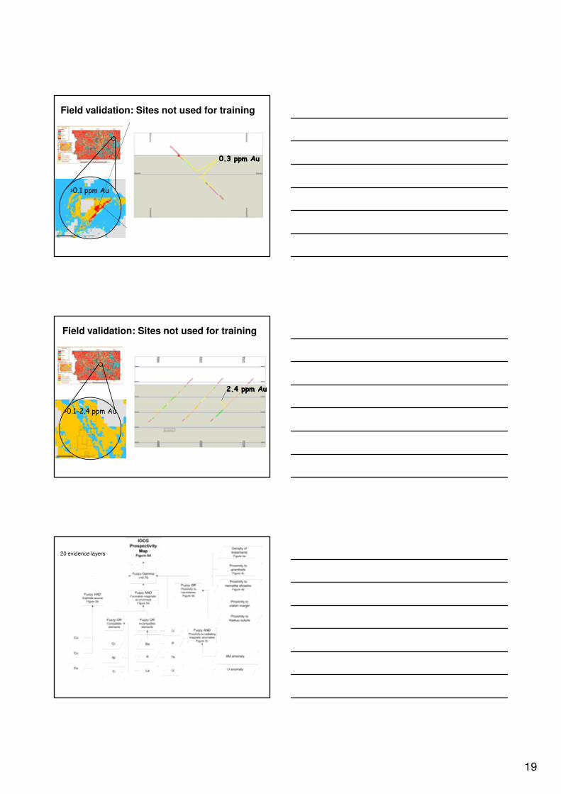
Field validation: Sites not used for training
0.3 ppm Au0.3 ppm Au
>0.1 ppm Au
Field validation: Sites not used for training
>0.1-2.4 ppm Au
2.4 ppm Au2.4 ppm Au
IOCG FUZZY MODEL20 evidence layers
20
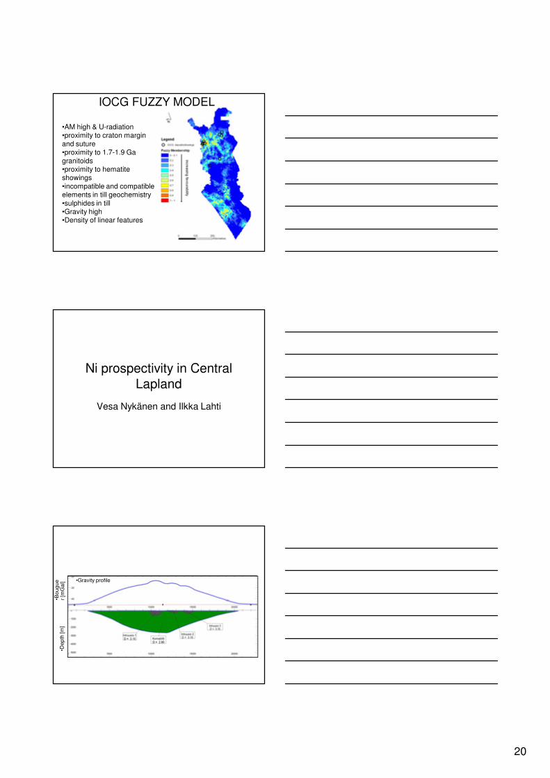
•AM high & U-radiation•proximity to craton margin
and suture•proximity to 1.7-1.9 Ga
granitoids•proximity to hematite showings
•incompatible and compatible elements in till geochemistry
•sulphides in till•Gravity high•Density of linear features
IOCG FUZZY MODEL
Ni prospectivity in Central
Lapland
Vesa Nykänen and Ilkka Lahti
•De
pth
[m
]•B
ou
gu
er
[mG
al] •Gravity profile

21
•High pass filter (cut off wavelength 5km)
•Gravity profile
•[m
Ga
l]•D
ep
th [m
]•B
ou
gu
er
[mG
al]
27°E
27°E
26°E
26°E
25°E
25°E
68°N
68°
N
67°5
0'N
67°5
0'N
67°4
0'N
67°40
'N
67°3
0'N
67°3
0'N
0 105Km
30°E
30°E
25°E
25°E
20°E
20°E
69°N
69
°N
66°N
66°N
63°N
63
°N
60°N
60°N
Mining concession
Claim (Ni-Cu)
Claim application
Reservation
Magnetic field total intensity
High : 17280
Low : -3014
•Magnetic field total intensity
•Lithologicalboundaries
27°E
27°E
26°E
26°E
25°E
25°E
68°N
68°
N
67°5
0'N
67°5
0'N
67°4
0'N
67°40
'N
67°3
0'N
67°3
0'N
0 105Km
30°E
30°E
25°E
25°E
20°E
20°E
69°N
69
°N
66°N
66°N
63°N
63
°N
60°N
60°N
Mining concession
Claim (Ni-Cu)
Claim application
Reservation
High pass AM
High : 17365.5
Low : -2847.5
•Magnetic field totalintensity
•High pass filterusing median value over 2 km radius neighborhood
22
27°E
27°E
26°E
26°E
25°E
25°E
68°N
68°
N
67°5
0'N
67°5
0'N
67°4
0'N
67°40
'N
67°3
0'N
67°3
0'N
0 105Km
30°E
30°E
25°E
25°E
20°E
20°E
69°N
69
°N
66°N
66°N
63°N
63
°N
60°N
60°N
Mining concession
Claim (Ni-Cu)
Claim application
Reservation
Gravity
Bouguer anomaly
High
Low
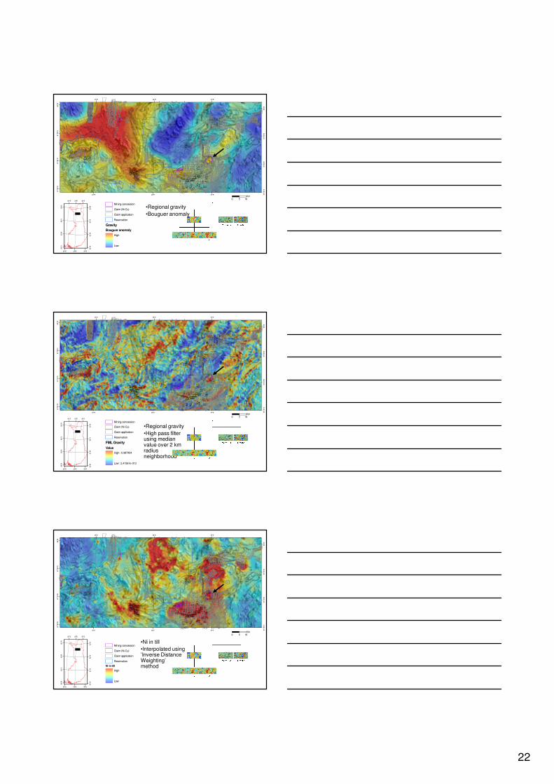
•Regional gravity
•Bouguer anomaly
27°E
27°E
26°E
26°E
25°E
25°E
68°N
68°
N
67°5
0'N
67°5
0'N
67°4
0'N
67°40
'N
67°3
0'N
67°3
0'N
0 105Km
30°E
30°E
25°E
25°E
20°E
20°E
69°N
69
°N
66°N
66°N
63°N
63
°N
60°N
60°N
Mining concession
Claim (Ni-Cu)
Claim application
Reservation
FML Gravity
Value
High : 0.997404
Low : 2.41361e-013
•Regional gravity
•High pass filter using median value over 2 km radiusneighborhood
27°E
27°E
26°E
26°E
25°E
25°E
68°N
68°
N
67°5
0'N
67°5
0'N
67°4
0'N
67°40
'N
67°3
0'N
67°3
0'N
0 105Km
30°E
30°E
25°E
25°E
20°E
20°E
69°N
69
°N
66°N
66°N
63°N
63
°N
60°N
60°N
Mining concession
Claim (Ni-Cu)
Claim application
Reservation
Ni in till
High
Low
•Ni in till
•Interpolated using ’Inverse DistanceWeighting’ method

23
27°E
27°E
26°E
26°E
25°E
25°E
68°N
68°
N
67°5
0'N
67°5
0'N
67°4
0'N
67°40
'N
67°3
0'N
67°3
0'N
0 105Km
30°E
30°E
25°E
25°E
20°E
20°E
69°N
69
°N
66°N
66°N
63°N
63
°N
60°N
60°N
Mining concession
Claim (Ni-Cu)
Claim application
Reservation
Ni in till (resid 6k)
High
Low
•Ni in till
•High pass filter using median value over 6 km radius neighborhood
27°E
27°E
26°E
26°E
25°E
25°E
68°N
68°
N
67°5
0'N
67°5
0'N
67°4
0'N
67°40
'N
67°3
0'N
67°3
0'N
0 105Km
30°E
30°E
25°E
25°E
20°E
20°E
69°N
69
°N
66°N
66°N
63°N
63
°N
60°N
60°N
Mining concession
Claim (Ni-Cu)
Claim application
Reservation
And till (Ni, Cu, Co)
High
Low
•Combined till geochemistry(Ni+Cu+Co)
27°E
27°E
26°E
26°E
25°E
25°E
68°N
68°
N
67°5
0'N
67°5
0'N
67°4
0'N
67°40
'N
67°3
0'N
67°3
0'N
0 105Km
30°E
30°E
25°E
25°E
20°E
20°E
69°N
69
°N
66°N
66°N
63°N
63
°N
60°N
60°N
Mining concession
Claim (Ni-Cu)
Claim application
Reservation
Ni prospectivity
Very low
Low
Moderate
High
Very high
•69•Vesa Nykänen, 27.4.2011
•Prospectivity map combining AM,gravity and till geochemistry

24
Summary
• This prospectivity model combined till geochemistry (Ni, Cu and Co) with airborne magnetics and regional
gravity
• The data was filtered using a high-pass filtering
technique, where long wave length signal is removed from the data resulting local anomalies
• Resulting prospectivity map identifies more than 40 targets areas favorable for Ni-Cu deposits
• Most of these areas are under active exploration
Coffee/Tea break
LAB 1
Navigating in ArcGISDisplaying data in a GIS

25
geology(1-of-n coded) magnetic anomalygamma-ray
channelsto tal countdistance to nearest faultK
ThU
input layerhiddenlayer
internal biases =
Map
1 9 sandstone Cambrian
2 6 rhyodacite E. Triassic
3 7 granite E. Triassic
4 4 leucogranite L. Triassic
Polygon Class Rock Type AgeAttributes
GIS software links the location
(map) data and the attribute data
N
WHAT IS GIS
Query
Analyze
Store Display
Capture
Output
What a GIS Does
Introducing ArcMAP
• Starting a ArcGIS Map Document
– From the start menu Programs->ArcGIS->ArcMAP
– Then select the document to open from the File Menu
26
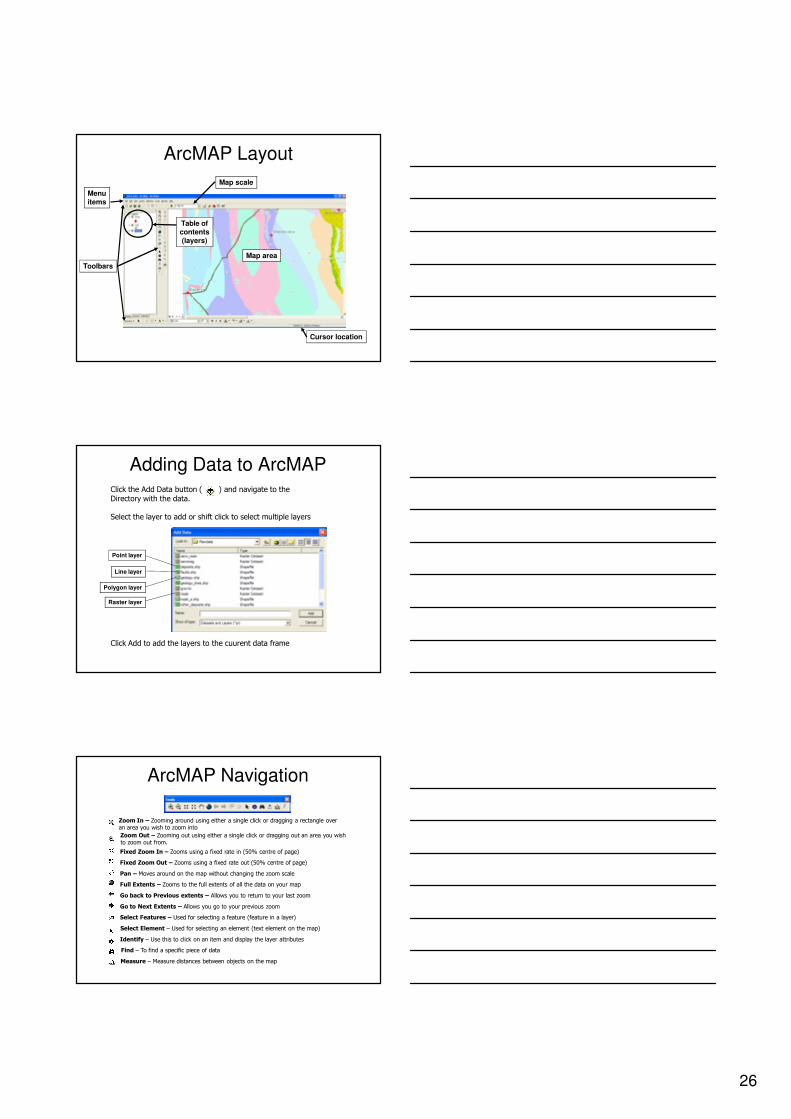
ArcMAP Layout
Table ofcontents(layers)
Map area
Cursor location
Toolbars
Menuitems
Map scale
Click the Add Data button ( ) and navigate to the Directory with the data.
Select the layer to add or shift click to select multiple layers
Adding Data to ArcMAP
Click Add to add the layers to the cuurent data frame
Point layer
Line layer
Polygon layer
Raster layer
Zoom In – Zooming around using either a single click or dragging a rectangle over an area you wish to zoom into
Zoom Out – Zooming out using either a single click or dragging out an area you wishto zoom out from.
Fixed Zoom In – Zooms using a fixed rate in (50% centre of page)
Fixed Zoom Out – Zooms using a fixed rate out (50% centre of page)
Pan – Moves around on the map without changing the zoom scale
Full Extents – Zooms to the full extents of all the data on your map
Go back to Previous extents – Allows you to return to your last zoom
Go to Next Extents – Allows you go to your previous zoom
Select Features – Used for selecting a feature (feature in a layer)
Select Element – Used for selecting an element (text element on the map)
Identify – Use this to click on an item and display the layer attributes
Find – To find a specific piece of data
Measure – Measure distances between objects on the map
ArcMAP Navigation
27
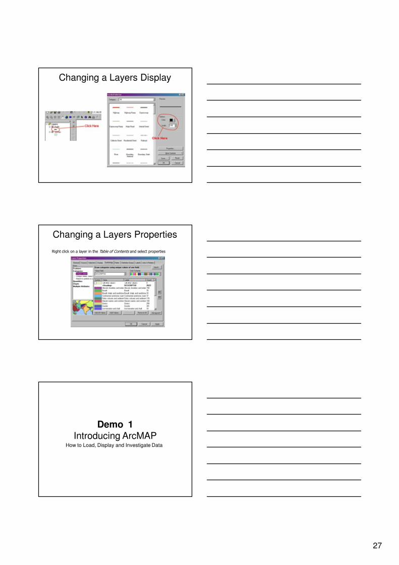
Changing a Layers Display
Changing a Layers Properties
Right click on a layer in the Table of Contents and select properties
Demo 1
Introducing ArcMAPHow to Load, Display and Investigate Data
28
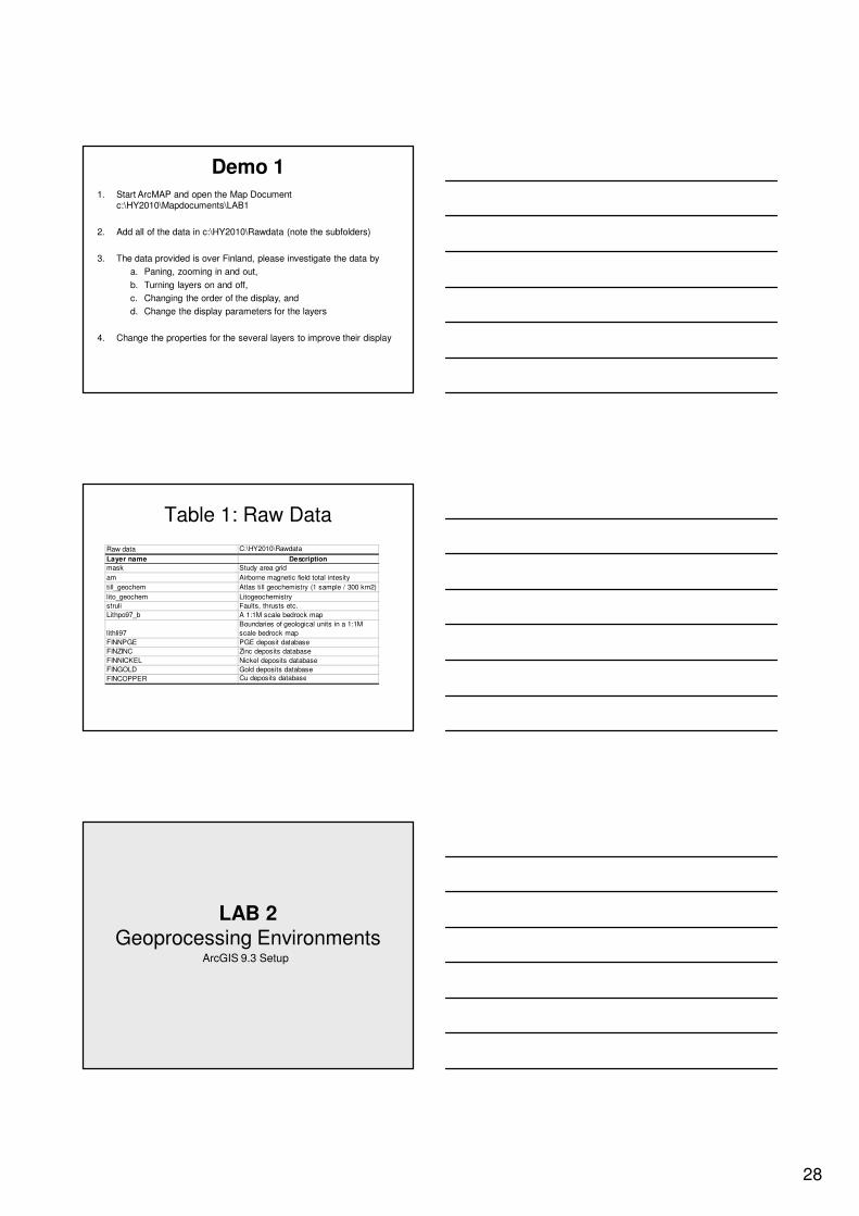
Demo 11. Start ArcMAP and open the Map Document
c:\HY2010\Mapdocuments\LAB1
2. Add all of the data in c:\HY2010\Rawdata (note the subfolders)
3. The data provided is over Finland, please investigate the data by
a. Paning, zooming in and out,
b. Turning layers on and off,
c. Changing the order of the display, and
d. Change the display parameters for the layers
4. Change the properties for the several layers to improve their display
Table 1: Raw Data
Raw data C:\HY2010\Rawdata
Layer name Description
mask Study area grid
am Airborne magnetic field total intesity
till_geochem Atlas till geochemistry (1 sample / 300 km2)
lito_geochem Litogeochemistry
struli Faults, thrusts etc.
Lithpo97_b A 1:1M scale bedrock map
lithli97
Boundaries of geological units in a 1:1M
scale bedrock map
FINNPGE PGE deposit database
FINZINC Zinc deposits database
FINNICKEL Nickel deposits database
FINGOLD Gold deposits database
FINCOPPER Cu deposits database
LAB 2
Geoprocessing EnvironmentsArcGIS 9.3 Setup

29
Introduction to ArcToolbox
• Environment
– Tools/Options
• ArcToolbox
• Model Building
Introduction
• Environment
– Tools/Options
• ArcToolbox
• Model Building
Tools/Options: Raster tab
• Raster Attribute Table
– Number of unique
conditions or records in the raster attribute table
limited to 65,536
– For Neural Network and
Logistic Regression tools, may need a larger value.
30
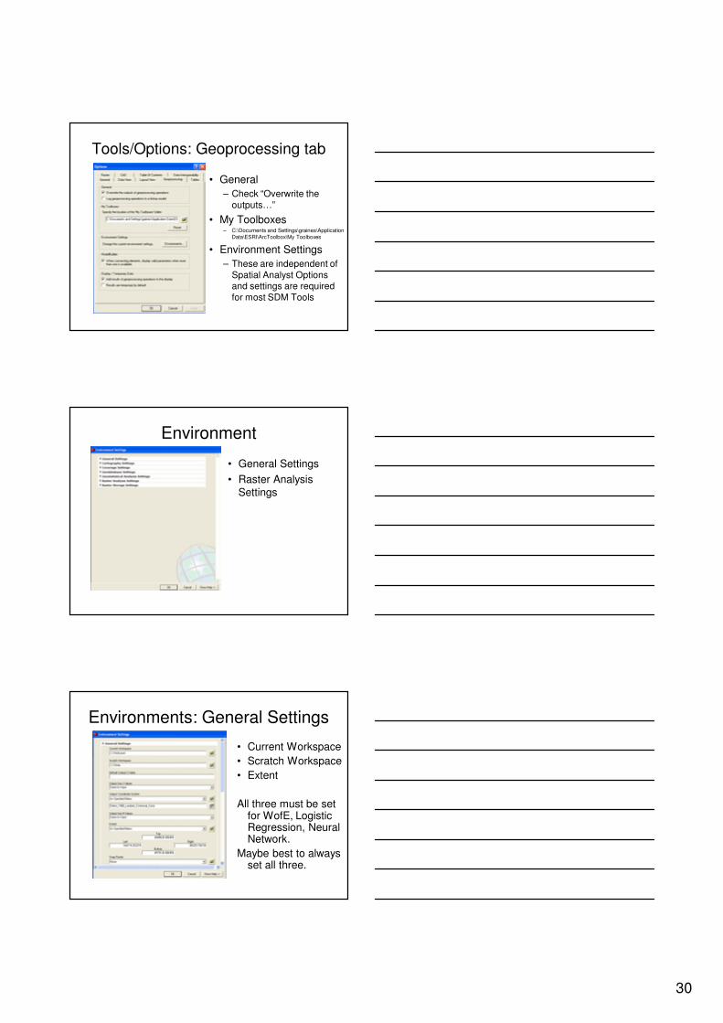
Tools/Options: Geoprocessing tab
• General
– Check “Overwrite the
outputs…”
• My Toolboxes– C:\Documents and Settings\graines\Application
Data\ESRI\ArcToolbox\My Toolboxes
• Environment Settings
– These are independent of
Spatial Analyst Options and settings are required
for most SDM Tools
Environment
• General Settings
• Raster Analysis
Settings
Environments: General Settings
• Current Workspace
• Scratch Workspace
• Extent
All three must be set for WofE, Logistic Regression, Neural Network.
Maybe best to always set all three.
31
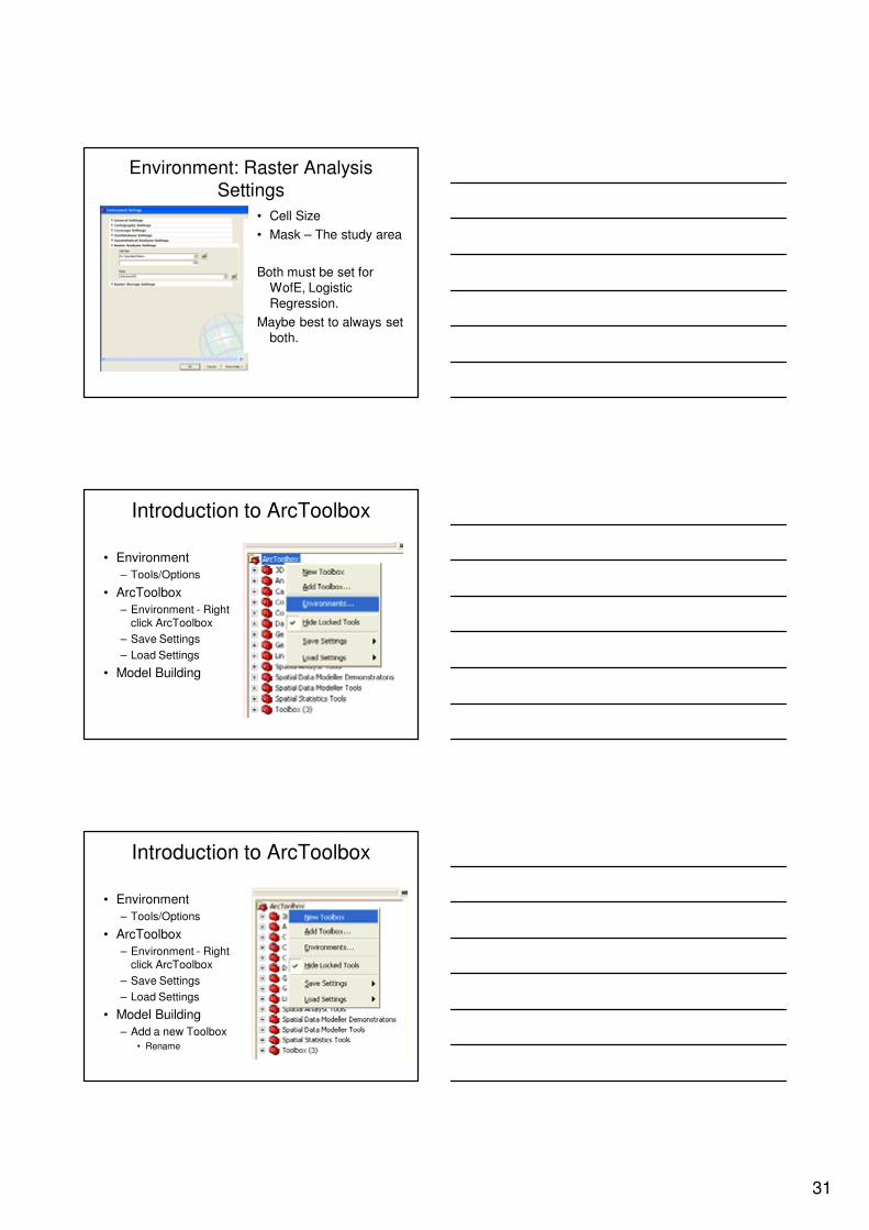
Environment: Raster Analysis
Settings
• Cell Size
• Mask – The study area
Both must be set for
WofE, Logistic
Regression.
Maybe best to always set
both.
Introduction to ArcToolbox
• Environment
– Tools/Options
• ArcToolbox
– Environment - Right click ArcToolbox
– Save Settings
– Load Settings
• Model Building
Introduction to ArcToolbox
• Environment
– Tools/Options
• ArcToolbox
– Environment - Right click ArcToolbox
– Save Settings
– Load Settings
• Model Building
– Add a new Toolbox
• Rename
32
Demo 2Geoprocessing Evironments
Setting the Parameters for all Subsequent GIS Processing
Demo 2• Start arcmap and open the Map Document
c:\HY2010\MapDocuments\Lab2
• Set the enviroment parameters
– The current workspace to c:\HY2010\Workspace
– The scratch workspace to c:\HY2010\Workspace\Temp
– Set the extent to c:\HY2010\RawData\mask
• What is the Mask data set?
• Define the following properties of the mask layer:
– Cell size?
– Total cells?
– Total area?
– Define the extent
• Min Easting?
• Max Easting?
• Min Northing?
• Max Northing?
LAB 3
Geoprocessing ToolsCreating Derived GIS Layers

33
Derived Layer Philosophy
Remote Sensing
Geophysics
Geochemistry
Geology
Garbage In,Garbage Out
Prospectivity Maps
GIS
Analyse / Combine
Prospectivity Maps
GIS
Analyse / Combine
Good Data In, Good Resource Appraisal Out
Remote Sensing
Geophysics
Geochemistry
Geology
Discrete and continuous data
• Discrete features– Distinct boundaries
– Stored as integer values
– Land use, zoning, vegetation,
– lakes, roads, rivers
• Continuous phenomena– Continuously changing values
– Stored as floating point values
– Elevation, noise pollution, rainfall,
– Slope and temperature
GRIDS
Cells, rows, and columns
0 1 2 3
3
2
1
0
Row
Column
Cell (2,3)
• Grid themes are an organized matrix of cells
• Cells are organized into rows and columns
• Rows and columns have an index position number
• Top left cell is at the 0,0 position
GRIDS

34
Value Attribute Table
Value attribute Table
Is a table associated with
Integer grids that contains
related information
GRIDS
Grid Layer Properties
• Cell size: Dimension,
Units
• Extent Rows, Columns
• Type: Boolean, Integer,
Floating
• Mask: No data
GRIDSArithmetic Operators

35
GRIDSEuclidean Feature
Spatial processing of grid cells, allow for distance, direction and
allocation of proximity
Euclidean FeatureGRIDS
Euclidean_distanceReturns distance to nearest feature
Euclidean_directionReturns direction to nearest feature
Euclidean_allocationReturns value of nearest feature
Inverse Distance Weighting
• Determines cell values using a weighted
combination of a set of sample points,
with the weight a function of inverse
distance.
• The further an input point is from the
output cell location, the less importance it
has in the calculation of the output value.
GRIDS
36
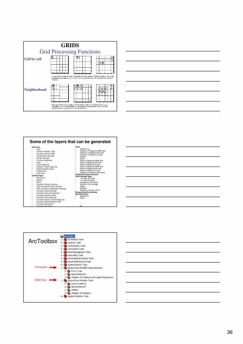
GRIDSGrid Processing Functions
Cell by cell
Neighborhood
Some of the layers that can be generatedHost rock
• Type• Young's modulus, CRC
• Young's modulus, AMC• Compressive Strength
• Tensile Strength
• Fracture toughness• Type
• Fe/(Fe+Mg+Ca)• Fe(wt%)* Fe/(Fe+Mg+Ca)
• Fe2O3/(Fe2O3+FeO)• Fe2O3/FeO
• Fe2+/Fe3+
Contact Type• distance to
• density• Strike
• Contrast Young's modulus, • CRC Contrast Young's modulus,
• AMC Contrast Compressive Strength
• Contrast Tensile Strength• Contrast Fracture toughness
• Contrast Chemical ratios• Contrast Fe/(Fe+Mg+Ca)
• Contrast Fe(wt%)* Fe/(Fe+Mg+Ca)• Contrast Fe2O3/(Fe2O3+FeO)
• Contrast Fe2O3/FeO
• Contrast Fe2+/Fe3+
Fault• Distance to• Distance of Regional NNW fault• Distance of Regional NE fault• Distance of Regional E fault• density• Strike• Strike of Regional NNW fault• Strike of Regional NE fault- Strike of Regional E fault• Strike of Regional NNW fault• Strike of Regional NE fault• Strike of Regional E fault• Distance to nearest intersectionPorphyritic felsic intrusionField strength data• +ve mag. Anomaly• -ve mag. Anomaly- average by Host Rock- Variation from average- Slope- Variation- Magnetic intensity (RTP)Bouguer gravity anomalySynclinal axes • distance to• Strike
…
etc
ArcToolbox
Training Aid
SDM Tools

37
Spatial Data
Modeller (SDM) toolbox
Geoprocessing tools for integration of spatial data to predict the location to any features
(i.e. mineral deposits, animal habitat,
disease outbreaks … etc).
SDM is available at the ESRI ArcScripts site :
http://arcscripts.esri.com/details.asp?dbid=15341
or at the University of Campinas site:
http://www.ige.unicamp.br/sdm/default_e.htm
Creating a New Toolbox
• Right click on Toolbox and select from the drop down menu New Toolbox
• A new toolset called ToolBox will be added
• To rename right click and select rename
• Use toolsets to store your processing models
Creating Models• Create a model in your tools right
click and add New Model
• Right click on your new model to:
– Rename
– Edit
– Properties
– Edit Documentation
• Help
– Open

38
Creating a Simple Model
• Drag Reclassify to your model
• Right click the Reclassify tool and select Open.
• Blue – Input data
• Orange – Process
• Green – Output data
Reclassify Tool
Right click open
or double click
Model Button Commands
Save
Cut
Copy
Paste
Add L
aye
r
Auto
Layo
ut
Full
Exte
nt
Zoom
in
Zoom
Out
Mag
nify
Tool
Pan
Continuo
us Z
oom
Navig
ate
Tool (?
??)
Sele
ct
Add C
onnectio
n
Run

39
Sharing Models
• User Toolboxes
– C:\Documents and Settings\graines\Application
Data\ESRI\ArcToolbox\My Toolboxes
– Location defined in Tools->Options
• Relative versus absolute paths
– In ArcMap
– In Models
• %Workspace%
• %ScratchWorkspace%
• Iteration for example Large%i%
Documentation of Models
• Documentation is useful to remind you about the model or to tell an associate
how to use your model.
– Right click the model and select Edit
Documentation
• Model Reports
Demo 3Creating Distance to Thrust Faults
Generate a distance grid to thrust fault and reclassify into ten classes

40
Demo 31. Start arcmap and open the Map Document
c:\HY2010\MapDocuments\Lab3
2. Create a new toolbox called MyTools
3. Generate a distance to Faults Layer, by follow these steps:
– Add a new model to MyTools and rename it to Dist_to_Faults
– Edit the new model and add the layer Struli97 (drag and drop)
– Add the Euclidean Distance tool (drag and drop) which is located in the Spatial Analyst toolbox and the Distance toolset
– Use the Add Connection tool to link the Struli97 to the Euclidean Distance in the model window
– Double click on either the Euclidean Distance or Output Distance to definethe Output Distance Raster, set the new name to beC:\HY2010\Workspace\Temp\Dist_faults
– Right click the Output Distance model and select Add to Display
– Save the model
– Run the Model
– Set the properties for the new layer to be red close to the faults and blueaway from the faults
Demo 34. Create a new model called Distance_to_GeologyLines (using the
same approach as question 3) that will generate a distance grid calledDist_geolines.
5. Create a new model call Density_of_Geolines that will be used to examine the association of gold minerisation to density of geologycontacts. In this model you need to load the Geology Lines layer and use Line Density tool in the Density Toolset located in the SpatialAnalyst Toolbox. Set the search radius to 2000m.
6. Create a new model call Density_of_Faults that will be used to examine the association of gold minerisation to areas of high faultintersections. In this model you need to load the Faults layer and useLine Density tool in the Density Toolset located in the Spatial AnalystToolbox. Set the search radius to 2000m.
7. Use the Till geochemisty, and the IDW tool in the Interpolation toolsetlocated in the Spatial Analyst Toolbox to generate a continuoussurface of the Cu chemistry _(set the Z value to Cu_312P). Use the default values for IDW
Table 1: Raw Data
Raw data C:\HY2010\Rawdata
Layer name Description
mask Study area grid
am Airborne magnetic field total intesity
till_geochem Atlas till geochemistry (1 sample / 300 km2)
lito_geochem Litogeochemistry
struli Faults, thrusts etc.
Lithpo97_b A 1:1M scale bedrock map
lithli97
Boundaries of geological units in a 1:1M
scale bedrock map
FINNPGE PGE deposit database
FINZINC Zinc deposits database
FINNICKEL Nickel deposits database
FINGOLD Gold deposits database
FINCOPPER Cu deposits database

41
Lunch
LAB 4
Weights of Evidence: trainingDefining sites to measure spatial associations
Weights-of-Evidence Method
• Originally developed as a medical diagnosis system
– relationships between symptoms and disease
evaluated from a large patient database
– each symptom either present/absent
– weight for present/weight for absent (W+/W-)
• Apply weighting scheme to new patient
– add the weights together to get result

42
Weights of Evidence - WofE
• Data driven technique
– Requires training sites
• Statistical calculations are used to derive
the weights based upon training sites.
• Evidence (maps) are generally reclassified
into binary patterns.
• Deposit location (binary grid)
• Deposit location > 1000 kg
Au (binary grid)
• Gold production (historic)
• Total contained gold (TCG)
Types of Deposit Layers
PAHTAVAARA
Central Lapland
Train Set Layer
• If Cell size is too small then
deposits resource layer has to be
subdivided.
• Cell size is too large deposit
associations have to be merged
Cell Size Problem
43
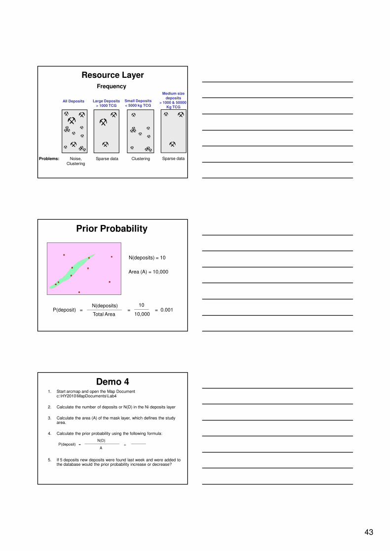
Resource Layer
Frequency
All Deposits Large Deposits
> 1000 TCG
Small Deposits
< 5000 kg TCG
Problems: Sparse data ClusteringNoise,Clustering
Medium size
deposits> 1000 & 50000
Kg TCG
Sparse data
Prior Probability
Area (A) = 10,000
N(deposits) = 10
= 10
10,000= 0.001
N(deposits)
Total AreaP(deposit) =
Demo 41. Start arcmap and open the Map Document
c:\HY2010\MapDocuments\Lab4
2. Calculate the number of deposits or N(D) in the Ni deposits layer
3. Calculate the area (A) of the mask layer, which defines the studyarea.
4. Calculate the prior probability using the following formula:
5. If 5 deposits new deposits were found last week and were added to the database would the prior probability increase or decrease?
= N(D)
AP(deposit) =

44
N(D) = 5
Conditional Probability
N(A) = 1,000
P(D | A) =
A
A ∩ D
A ∩ D
D N(total) = n = 10,000
A ∩ D
greenstone deposits
Definition of conditional probability
P(D ∩∩∩∩ A)
P(A)
greenstone
A ∩ D
A ∩ D
N(D ∩∩∩∩ A) / n
N(A) / n= =
N(D ∩∩∩∩ A) = 5
5
1000= 0.005
(in greenstone)A ∩ D
Deposit cells = 5
Posterior Probability
Greenstone cells = 1,000
P(deposit | greenstone present) = P(deposit) x F+, where A+ > 1
P(deposit | greenstone absent) = P(deposit) x F-, where A+ < 1
prior
Posterior
Conditional Probability and Bayes’ Rule
Bayes’ Rule
P(D | A) = P(D ∩∩∩∩ A)
P(A)
P(A | D )
P(A)P(D | A) = P(D)
priorposterior (conditional)
probability
update factor
P(A | D )
P(A)P(D | A) = P(D) Case where favourable
pattern is absent

45
Weights-of-Evidence Terms
• Weights for patterns
W+ - weight for inside the pattern
W- - Weight for outside the pattern
0 - Weights for areas of no data
• Contrast - a measure of the spatial
association of pattern with sites
• Studentized Contrast - a measure of the
significance of the contrast
Weights of Evidence
• Binary maps to define favorable areas
–Can use multi-layer patterns
• Measurements
–Area of study
–Area of Pattern
–Number of training sites
–Number of training sites inside the pattern
Application to Binary Evidence
1 2
1 50 8 0.8/0.5=1.6 ln(1.6)= +0.47
2 50 2 0.2/0.5=0.4 ln(0.4)= -0.92
Total 100 10
Class Area #sites Relative density Weight
46
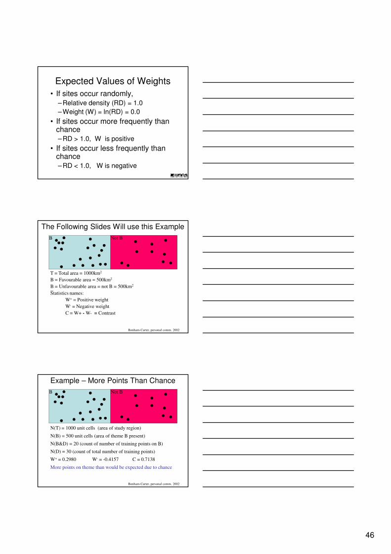
Expected Values of Weights
• If sites occur randomly,
–Relative density (RD) = 1.0
–Weight (W) = ln(RD) = 0.0
• If sites occur more frequently than chance
–RD > 1.0, W is positive
• If sites occur less frequently than chance
–RD < 1.0, W is negative
The Following Slides Will use this Example
T = Total area = 1000km2
B = Favourable area = 500km2
B = Unfavourable area = not B = 500km2
Statistics names:
W+ = Positive weight
W- = Negative weight
C = W+ - W- = Contrast
B Not B
Bonham-Carter, personal comm. 2002
Example – More Points Than Chance
N(T) = 1000 unit cells (area of study region)
N(B) = 500 unit cells (area of theme B present)
N(B&D) = 20 (count of number of training points on B)
N(D) = 30 (count of total number of training points)
W+ = 0.2980 W- = -0.4157 C = 0.7138
More points on theme than would be expected due to chance
B Not B
Bonham-Carter, personal comm. 2002
47
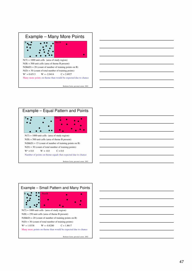
Example – Many More Points
N(T) = 1000 unit cells (area of study region)
N(B) = 500 unit cells (area of theme B present)
N(B&D) = 28 (count of number of training points on B)
N(D) = 30 (count of total number of training points)
W+ = 0.6513 W- = -2.0414 C = 2.6927
Many more points on theme than would be expected due to chance
B Not B
Bonham-Carter, personal comm. 2002
Example – Equal Pattern and Points
N(T) = 1000 unit cells (area of study region)
N(B) = 500 unit cells (area of theme B present)
N(B&D) = 15 (count of number of training points on B)
N(D) = 30 (count of total number of training points)
W+ = 0.0 W- = -0.0 C = 0.0
Number of points on theme equals that expected due to chance
B Not B
Bonham-Carter, personal comm. 2002
Example – Small Pattern and Many Points
N(T) = 1000 unit cells (area of study region)
N(B) = 250 unit cells (area of theme B present)
N(B&D) = 20 (count of number of training points on B)
N(D) = 30 (count of total number of training points)
W+ = 1.0338 W- = -0.8280 C = 1.8617
Many more points on theme than would be expected due to chance
B Not B
Bonham-Carter, personal comm. 2002

48
Example - Weights Undefined
N(T) = 1000 unit cells (area of study region)
N(B) = 250 unit cells (area of theme B present)
N(B&D) = 30 (count of number of training points on B)
N(D) = 30 (count of total number of training points)
W+ = inf W- = -inf C = inf
Undefined: practical solution--assign fraction of point to (not B)
B Not B
Bonham-Carter, personal comm. 2002
Multi-class Themes
• Maps (themes) with unordered classes
(categorical) e.g. geological map. Calculate
weights for each class and then group classes
(reclassify) as needed.
• Maps (themes) with ordered classes (contour
maps e.g. geochemical or geophysical field
variables). Usually calculate weights based on
successive contour levels, cumulatively. Then
reclassify.
Bonham-Carter, personal comm. 2002
Multi-class – Categorical Classes
N(T) = 1000 unit cells (area of study region)
N(A) = 250 , N(B) = 500, N(C) = 250,
N(A&D) = 23, N(B&D) = 4, N(C&D) = 3,
N(D) = 30 (count of total number of training points)
W1 = 1.1866 W2 = -1.3442 W3 =-0.9347 Cmax =2.5308
Three classes, e.g. rock types (categorical scale of measurement)
A B C
Bonham-Carter, personal comm. 2002
Inside
Pattern
Outside
Pattern
49
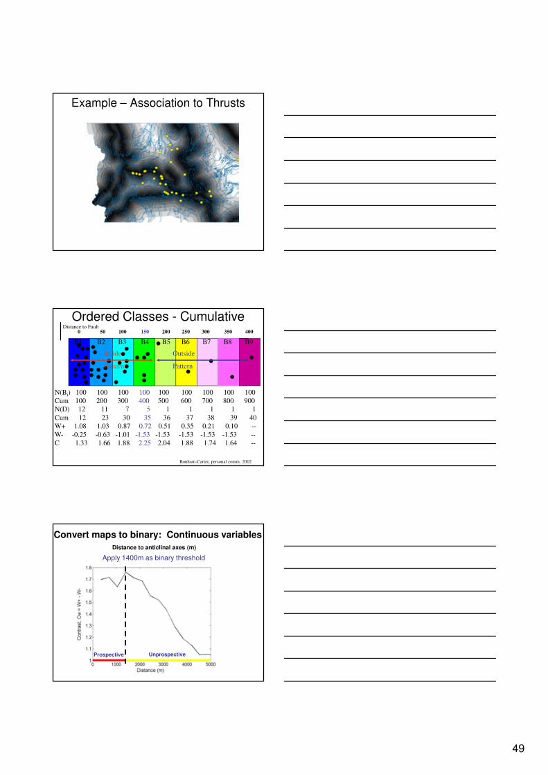
Example – Association to Thrusts
Ordered Classes - Cumulative
B1 B
2B3
B2 B3 B4 B5 B6 B7 B8 B9
0 50 100 150 200 250 300 350 400
Bonham-Carter, personal comm. 2002
Inside
Pattern
Outside
Pattern
N(Bi) 100 100 100 100 100 100 100 100 100
Cum 100 200 300 400 500 600 700 800 900
N(D) 12 11 7 5 1 1 1 1 1
Cum 12 23 30 35 36 37 38 39 40
W+ 1.08 1.03 0.87 0.72 0.51 0.35 0.21 0.10 --
W- -0.25 -0.63 -1.01 -1.53 -1.53 -1.53 -1.53 -1.53 --
C 1.33 1.66 1.88 2.25 2.04 1.88 1.74 1.64 --
Distance to Fault
Convert maps to binary: Continuous variables
Apply 1400m as binary threshold
Distance to anticlinal axes (m)
Prospective Unprospective

50
Thrusts Association to Deposits
1. Create new weights model
2. Add (drag and drop)
Calculate Weights tool into
new model
3. Add distance to thrusts
layer
Example – Create Model
1. Set Type
• Cumulative Ascending weights
(from lowest to highest value),
• Cumulative Descending
weights (from highest to lowest
value), or
• Categorical (unique for each
class)
2. Set Output Weights Table
(generates a dbf file of weights)
3. Set Confidence Level of
Studentized Contrast. The default
value is 2 (>98% confidence)
Example – Create Model
51
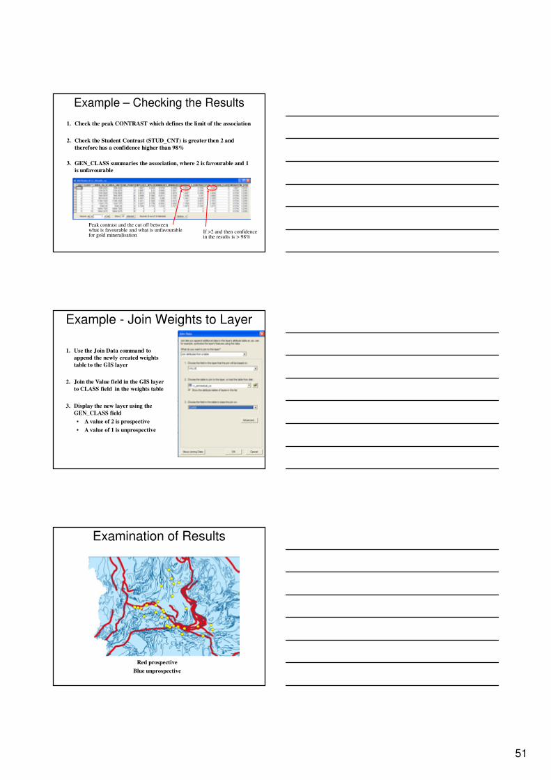
Example – Checking the Results
1. Check the peak CONTRAST which defines the limit of the association
2. Check the Student Contrast (STUD_CNT) is greater then 2 and
therefore has a confidence higher than 98%
3. GEN_CLASS summaries the association, where 2 is favourable and 1
is unfavourable
Peak contrast and the cut off between what is favourable and what is unfavourable for gold mineralisation
If >2 and then confidence in the results is > 98%
Example - Join Weights to Layer
1. Use the Join Data command to
append the newly created weights
table to the GIS layer
2. Join the Value field in the GIS layer
to CLASS field in the weights table
3. Display the new layer using the
GEN_CLASS field
• A value of 2 is prospective
• A value of 1 is unprospective
Examination of Results
Red prospective
Blue unprospective

52
Demo 5Calculating Weights
Calculate the Weights from the Distance to Thrust Layer
Demo 51. Start arcmap and open the Map Document
c:\HY2010\MapDocuments\Lab5
2. Create a new toolbox called MyTools
3. Create a new tool Struct_Weights, and
a. Add (drag and drop) the Calculate Weights tool in the Weights of Evidence toolset located in the SDM toolbox,
b. Add density of structures layer (rcdnsstruli) to the model and link to the Calculate Weights tool using the add connection
c. Double click the calculate weights tool in the model to set the training points field to Au deposits (orogenic_gold)
d. Set the association type to be descending (as the deposits occur in areas with high density of faults)
e. Set the output weights table to be rcdnsstruli_CD.dbf
f. Leave the other input fields to the default settings
g. Click apply and OK
h. Run the model
Demo 54. Load the rcdst2struli_CD.dbf which is located in the
HY2010\workspace and open the table and answer the following questions (Note: the table may already be loaded if you have set the tools properties to add to display) :
a. Which class has the highest Contrast (see the CONTRAST field)?
b. What is the significance of the highest contrast value?
c. How many deposits occur in the favourable region (see the NO_POINTS field).
d. What is the total area in the favourable region?
e. If the student contrast (STUD_CNT) is a measure of the statistical confidence of a result, Using Table 1, provided on the next slide, to calculate the statistical confidence of the highest contrast?
f. Add the table c:\HY2010\Derived\ rcdnsstruli to load the distance values assigned with each class. Exam this table and comment on what is the critical distance away from a thrust that controls the location of the deposits. Note the CLASS field in rcdnsstruli_CD.dbf matches the ROWID in rcdnsstruli table

53
Table 1: Student T Values
Confidence T Value
99.5% 2.576
99% 2.326
97.5% 1.96
95% 1.645
90% 1.282
80% 0.842
70% 0.542
60% 0.253
Demo 54. Create a new model, as document in question 3, to investigate
the domain boundary layer (rcdst2domli) and determine the following:
a. Which class has the highest Contrast (see the CONTRAST field)?
b. What is the significance of the highest contrast value?
c. How many deposits occur in the favourable region (see the NO_POINTS field).
d. What is the total area in the favourable region?
e. What is the statistical confidence of the highest contrast?
f. Add the associated weights table (see table 2) and detereminewhat is the critical distance away from a fault?
g. Which is the better layer for controlling the distribution of the deposits, the ’Struli’ layer or the ’domli’ layer?
LAB 6
Generate Prospectivity MapCombine the Weights of Evidence Layers into a
Prospectivity Map
54
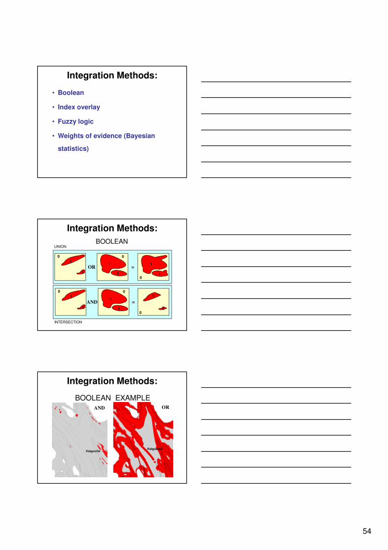
• Boolean
• Index overlay
• Fuzzy logic
• Weights of evidence (Bayesian
statistics)
Integration Methods:
BOOLEAN
0
1
1
02
1
1
0
1
1
OR =
01
1
AND
0
1
1
0
1
1
=
Integration Methods:
UNION
INTERSECTION
BOOLEAN EXAMPLE
AND OR
Integration Methods:
55
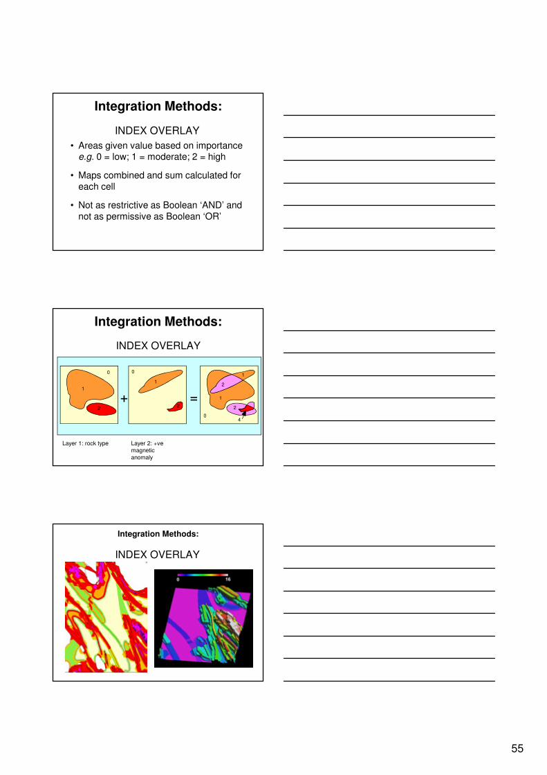
INDEX OVERLAY
• Areas given value based on importance e.g. 0 = low; 1 = moderate; 2 = high
• Maps combined and sum calculated for
each cell
• Not as restrictive as Boolean ‘AND’ and
not as permissive as Boolean ‘OR’
Integration Methods:
INDEX OVERLAY
0
1
1
2
2
4
0
1
2
0
1
2+ =
Integration Methods:
Layer 1: rock type Layer 2: +ve magnetic
anomaly
INDEX OVERLAY
Integration Methods:

56
Generate Weights Prospectivity
• Add the weights tables to the Table of Contents
• Create a new model
• Load the input layers into the
model (click and drag)
• Add the Calculate Response
tool located on the SDM
toolbox and the Weights of Evidence toolset
Calculate Response Tool
• Add the evidence Raster layers, either loading them from
the Calculate Response menu
or using the Add Connection Tool
• Load the weights tables, ensure
that the order is the same as the evidence layers.
• Set the Input Training Sites
Feature Class to be the
trainings sites.
• Output_Post_Prob_Raster: The posterior probabilty response raster created from the sum of the weights.
• Output_Prob_Std_Dev_Raster: Standard deviation due to the weights. If there is no missing data, this will also be the total standard deviation for the response raster.
• Output_MD_Variance_Raster: Variance due to missing data. This raster will only be calculated when missing data are expllicitly defined in at least one evidence layer.
• Output_Total_Std_Dev_Raster: Total standard deviation due to the weights and missing data. This raster will only be provided when there is explicitly defined missing data in at least one evidence layer.
• Output_Confidence_Raster: A raster showing the confidence that the reported posterior probability is not zero. This is the posterior probability divided by the total standard deviation, an approximite Student T test.
Calculate Response Tool
57
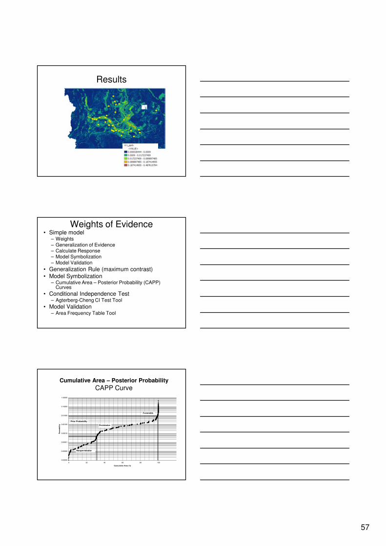
Results
Weights of Evidence• Simple model
– Weights
– Generalization of Evidence– Calculate Response– Model Symbolization
– Model Validation
• Generalization Rule (maximum contrast)
• Model Symbolization– Cumulative Area – Posterior Probability (CAPP)
Curves
• Conditional Independence Test– Agterberg-Cheng CI Test Tool
• Model Validation– Area Frequency Table Tool
Cumulative Area – Posterior Probability
CAPP Curve
0.00000
0.00000
0.00001
0.00010
0.00100
0.01000
0.10000
1.00000
0 20 40 60 80 100
Cumulative Area (%)
Favo
rab
ilit
y
Nonpermissive
Permissive
Favorable
Prior Probability

58
Demo 6Calculate Prospectivity Map
Calculate the Posterior Probabilty Using the Calulate Response Tool
Demo 61. Start arcmap and open the Map Document
c:\HY2010\MapDocuments\Lab6
2. Located in the Labtools toolbox are several tools, in thisexercise you will create several prospectivity maps using the Weights of evidence model
Open the Weights of evidence model tool, examine the modeland answer the following question
– How may evidence layers (or input layers) are used in the model?
– The thrust/fault layer (rcdnsstrulist) is an ascending or descendingassociation type in the calculate weights tool and why?
– Why is the till geochemisty (rc_till_cu) the opposite association typeto the thrust layer?
– What is the name of the prospectivity map generated?
– What is confidence value (the default value) used in the calculations of the weights?
– What is the name of the confidence map generated?
– Values above 2 in the confidence map are reliable or unreliable?
Demo 63. Delete two of the layers, which you regard as poor layers, from the
Weights of evidence model. You will also have to delete the associated calculate weights tools that were connected to the input layers you have deleted. When you have finnished editting the model then run. Running the model will take 5-10 minutes.
This will take between 5-10 minutes please use the time to have a coffee break
4. After the weights prospectivity map has been generated use the properties tool to recolour and better present your results.
5. Load the area frequency table, and investigate the data. This table documents how effect you prospective map is. How many deposits were captaured in the top 5% of the map?
6. Re-run the model with different input layers and investigate the results, which group of layers produce the best results.
59
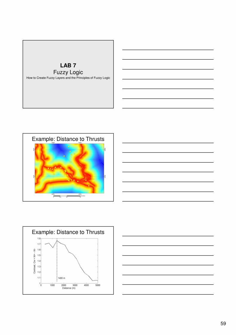
LAB 7
Fuzzy LogicHow to Create Fuzzy Layers and the Principles of Fuzzy Logic
Example: Distance to Thrusts
Example: Distance to Thrusts

60
Example: Distance to ThrustsBinary LayerBinary Layer
Define Association to Deposits
Objective Fuzzy Membership Layer
1.0
0.1
0 0.467P(deposit)

61
• “stream sediment gold concentration is anomalous”
variable µ fuzzy set
• fuzzy membership function, µ [0, 1]
• value membership degree
< 2 ppb 0.0
2 - 5 ppb 0.5
> 5 ppb 1.0
• m/ship values assigned subjectively
Fuzzy Logic
Fuzzy membership: Favorable for Au?
0.0
0.1
0.2
0.3
0.4
0.5
0.6
0.7
0.8
0.9
1.0
0 50 100 150 200 250 300 350 400
Pathfinder element (concentration)
Fu
zzy M
em
bers
hip
No
Yes
Missing Data or Uncertain
Probably
No
Probably
Yes
Fuzzy membership: Favorable for Au?
0.0
0.1
0.2
0.3
0.4
0.5
0.6
0.7
0.8
0.9
1.0
0 50 100 150 200 250 300 350 400
Pathfinder element (concentration)
Fu
zzy M
em
bers
hip
No
Yes
Missing Data or Uncertain
Probably
No
Probably
Yes

62
FUZZY INDEX OVERLAY
• Areas given value in range [0,1]
• based on degree of membership of fuzzy set:
importance
– 0 => definitely NOT favourable
– intermediate values => degrees of favourability
– 1 => definitely favourable
• Maps combined by using the Raster Calculator
Integration Methods:
FUZZY INDEX OVERLAY
+ =
Integration Methods:
0.5
0
1
0 0
1 1 1
0.5 0.5 1 1 1
1 1 1
1 1 2 2 2
1.5 1.5 1.5
1 1 1
Fuzzy membership values in range [0,1] ; added
Weighted fuzzy index overlay
(Map1 x weight 1) + (Map2 x weight 2) = Output map
0.5
0
1
0 0
1 1 1
0.5 0.5 1 1 1
1 1 1
1 1
x 4 x 1
+ =2
0
4
0 0
1 1 1
1 1 1
1 1 1
4 4 5 5 5
3 3 3
1 1 1
2 2
63
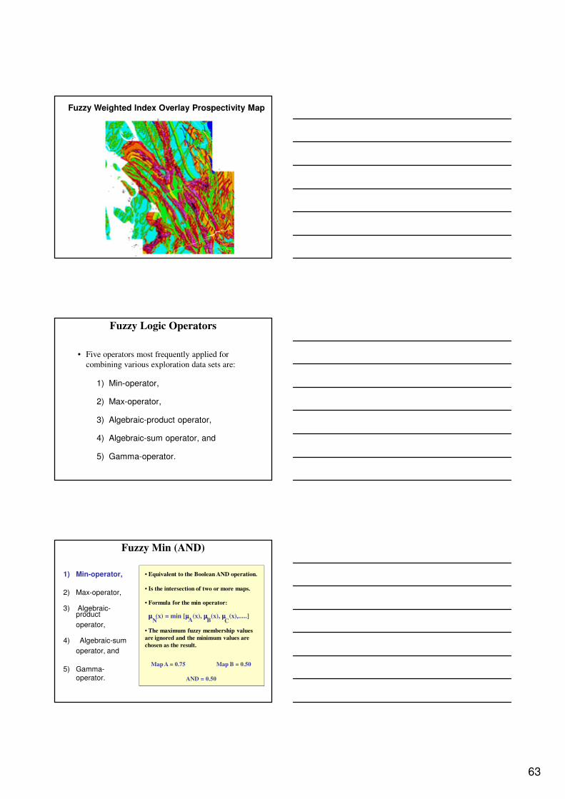
Fuzzy Weighted Index Overlay Prospectivity Map
1) Min-operator,
2) Max-operator,
3) Algebraic-product operator,
4) Algebraic-sum operator, and
5) Gamma-operator.
• Five operators most frequently applied for
combining various exploration data sets are:
Fuzzy Logic Operators
1) Min-operator,
2) Max-operator,
3) Algebraic-product
operator,
4) Algebraic-sum
operator, and
5) Gamma-operator.
• Equivalent to the Boolean AND operation.
• Is the intersection of two or more maps.
• Formula for the min operator:
• The maximum fuzzy membership values
are ignored and the minimum values are
chosen as the result.
Map A = 0.75 Map B = 0.50
AND = 0.50
µµµµ (x) = min [µµµµ (x), µµµµ (x), µµµµ (x),.....]N B CA
Fuzzy Min (AND)

64
EXAMPLE: Fuzzy Min (AND)
• Equivalent to the Boolean OR operation.
• Is the union of two or more maps.
• Formula for the max operator:
• The maximum fuzzy membership
values control the output map
occurring at each location and the
minimum values are ignored.
Map A = 0.75 Map B = 0.50
OR = 0.75
µ (x) = max [µ (x), µ (x), µ (x),.....]N B CA
Fuzzy Max (OR)
1) Min-operator,
2) Max-operator,
3) Algebraic-product
operator,
4) Algebraic-sum
operator, and
5) Gamma-operator.
EXAMPLE: Fuzzy Max (OR)
65
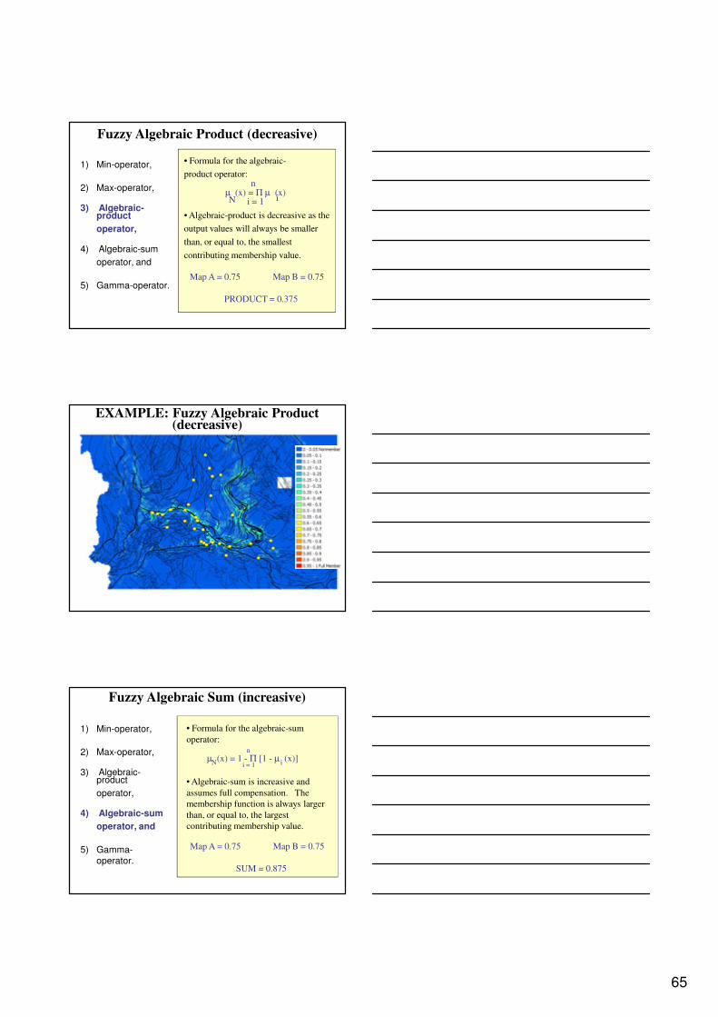
• Formula for the algebraic-
product operator:
• Algebraic-product is decreasive as the
output values will always be smaller
than, or equal to, the smallest
contributing membership value.
Map A = 0.75 Map B = 0.75
PRODUCT = 0.375
µ (x) = Π µ (x)N i = 1
n
i
Fuzzy Algebraic Product (decreasive)
1) Min-operator,
2) Max-operator,
3) Algebraic-product
operator,
4) Algebraic-sum
operator, and
5) Gamma-operator.
EXAMPLE: Fuzzy Algebraic Product (decreasive)
• Algebraic-sum is increasive and
assumes full compensation. The
membership function is always larger
than, or equal to, the largest
contributing membership value.
Map A = 0.75 Map B = 0.75
SUM = 0.875
µ (x) = 1 - Π [1 - µ (x)]N i = 1
n
i
• Formula for the algebraic-sum
operator:
Fuzzy Algebraic Sum (increasive)
1) Min-operator,
2) Max-operator,
3) Algebraic-product
operator,
4) Algebraic-sum
operator, and
5) Gamma-operator.
66
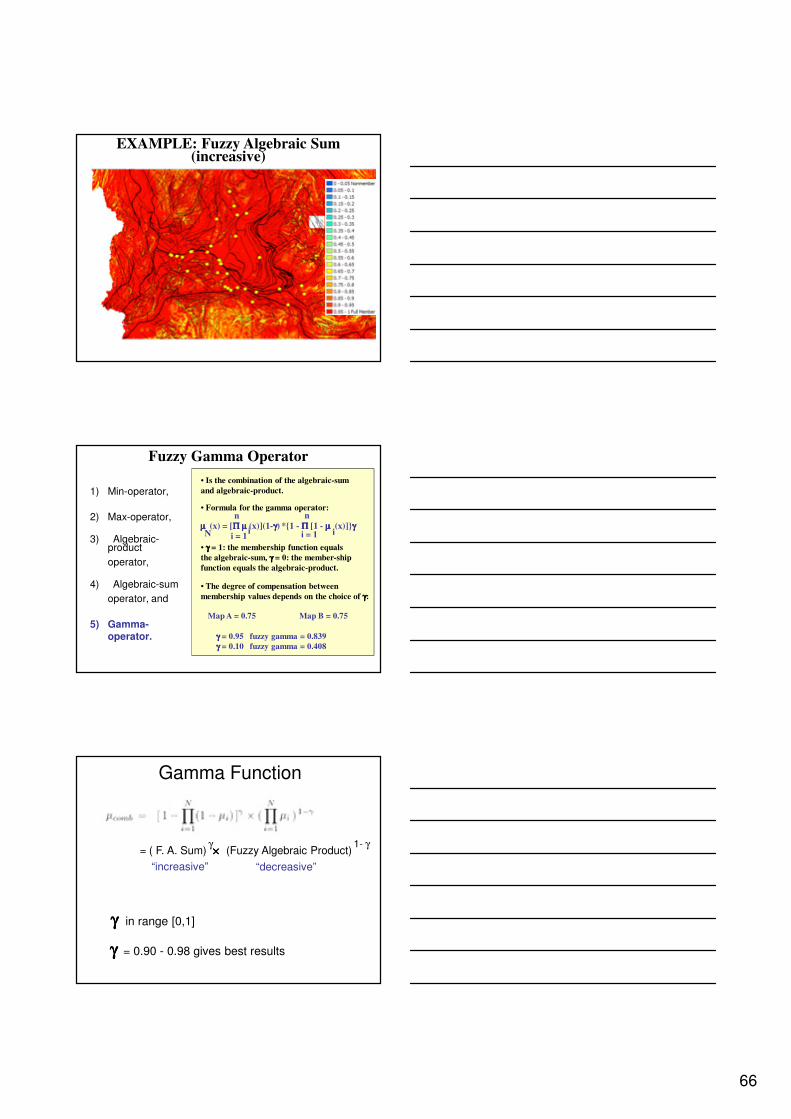
EXAMPLE: Fuzzy Algebraic Sum (increasive)
• γγγγ = 1: the membership function equals
the algebraic-sum, γγγγ = 0: the member-ship
function equals the algebraic-product.
Map A = 0.75 Map B = 0.75
γγγγ = 0.95 fuzzy gamma = 0.839
γγγγ = 0.10 fuzzy gamma = 0.408
• Formula for the gamma operator:
• Is the combination of the algebraic-sum
and algebraic-product.
µµµµ (x) = [ΠΠΠΠ µµµµ (x)](1-γγγγ) *{1 - ΠΠΠΠ [1 - µµµµ (x)]}γγγγN i = 1
n
ii = 1
n
i
• The degree of compensation between
membership values depends on the choice of γγγγ:
Fuzzy Gamma Operator
1) Min-operator,
2) Max-operator,
3) Algebraic-product
operator,
4) Algebraic-sum
operator, and
5) Gamma-operator.
Gamma Function
= ( F. A. Sum) ×××× (Fuzzy Algebraic Product)
“increasive”
γγγγ in range [0,1]
γ 1- γ
“decreasive”
γγγγ = 0.90 - 0.98 gives best results
67
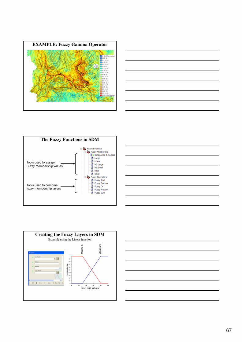
EXAMPLE: Fuzzy Gamma Operator
The Fuzzy Functions in SDM
Tools used to assignFuzzy membership values
Tools used to combine fuzzy membership layers
Creating the Fuzzy Layers in SDM
Min
imu
m
Ma
xim
um
Input Grid Values
Example using the Linear function

68
Using Fuzzy Operators in SDM
Layers to combine usingthe gamma functions
The gamma value used
Tools used to combine fuzzy membership layers
Example using the Gamma function
Demo 7Fuzzy Logic
Calculate Fuzzy Layer and Generate Fuzzy Prospectivity Maps
Demo 71. Start arcmap and open the Map Document c:\HY2010\MapDocuments\Lab7
2. Experiment with the fuzzy membership to generate fuzzy layers for the faultdensity and contact density layers.
3. Table 1, on the next slide, lists all of the fuzzy layers available, use the RasterCalculate to add several layers together (i.e. ”FM_tillcu + FM_tillas + … + FM_amres2”). The Raster calculator is located on the drop down menu of the Spatial Analyst tool bar. The resulting layer will be an index overlay map. Examine the result and comment on 1. how effective the result is? 2. What is the highest value in the map generated?
4. Run the Fuzzification 1 tool in the LabTools Toolbox and examine the results. What are the pros and cons of each of the fuzzy layers generated (you will haveto investigate the model to know what files are being generated)?
5. Create your own Gamma Funtion model and experiment with changing the gamma value. What happens when you increase or decrease the gamma value?

69
Table 1: Layers used in this Exercise
Layer name Description
FM_tillcu Interpolated (IDW) surface of Cu
FM_tillas Interpolated (IDW) surface of As
FM_dnsstruli Density of faults
FM_lithodiv Lithodiversity
FM_amres2
Residual grid after subtracting median value
over 4 km radius neighborhood of airborne
magnetics
Layers are located in C:\HY2010\Derived\Fuzzy
Coffee/tea
LAB 8
Neural NetworkThe Principles of Neural Networks in Prospectivity Mapping

70
What are artificial neural networks?
• adaptive computer systems
• can learn from data
• can generalise to new data
NN applications: industrial and commercial
Commercial
• credit card applications and detection of fraud• prediction of stock prices
• real estate valuation
Industrial
• automated face-detection• speech recognition
• automated recognition of hand-written post-codes
• industrial process control - e.g. sheet metal mill• control of unmanned aircraft - helicopters
• reconfigurable flight control systems - compensate for unknown damage
• recognition of features in MRI images of heart valves• EEG-based diagnosis of neurological and psychiatric disorders
• signal processing - filters to recover clean tone bursts from time signals
NN applications: exploration
• porosity and permiability prediction from wire-line logs
• lithology classifiaction from wire-line logs
• seismic facies classification
• prediction of oil and gas recovery
Petroleum exploration
• interpretation of three component downhole TEM data
• identification of anomalies - SOM, Neural Mining Solutions
• clustering stream sediment geochemical data
• classification of deposits (deposit models - ore mineralogy)
Mineral exploration
71
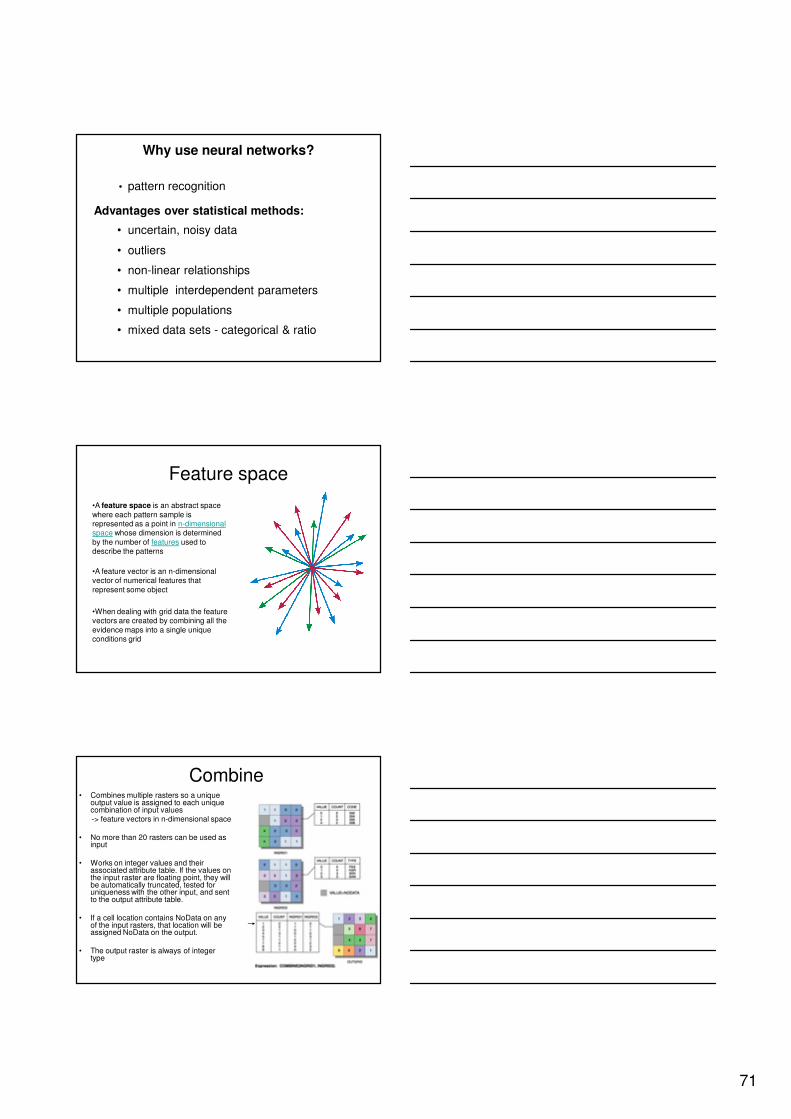
Why use neural networks?
• uncertain, noisy data
• outliers
• non-linear relationships
• multiple interdependent parameters
• multiple populations
• mixed data sets - categorical & ratio
• pattern recognition
Advantages over statistical methods:
Feature space
•A feature space is an abstract space
where each pattern sample is represented as a point in n-dimensional space whose dimension is determined
by the number of features used to describe the patterns
•A feature vector is an n-dimensional vector of numerical features that
represent some object
•When dealing with grid data the feature vectors are created by combining all the
evidence maps into a single unique conditions grid
Combine• Combines multiple rasters so a unique
output value is assigned to each unique combination of input values -> feature vectors in n-dimensional space
• No more than 20 rasters can be used as input
• Works on integer values and their associated attribute table. If the values on the input raster are floating point, they will be automatically truncated, tested for uniqueness with the other input, and sent to the output attribute table.
• If a cell location contains NoData on any of the input rasters, that location will be assigned NoData on the output.
• The output raster is always of integer type

72
Limitations in using GeoXplorer
• Max number of unique conditions (i.e. feature vectors) is ~200 000– Workarounds:
• Decrease the size of your study area -> tedious if resulting into lots of sub-areas to be combined
• Increase the cell size of your evidence -> loss of information
• Generalize your evidence data by classifying into a limited number of classes -> disturbs the original clustering in the data
-> all solutions have some sort of disturbance
Limitations in using GeoXplorer
• Max number of random sampling size in fuzzy clustering is 1000 (500 + 500)
– Workarounds:
• No real workaround except decrease the size of your study area -> tedious if resulting into lots of
sub-areas to be combined
– When less than 1000 unique conditions use
the same number of random sampling sites
as the number of unique conditons
Architecture of an MLP neural network
Input layer
hidden layer
output layer
y
x1
x3
x2
weight
73
geology(1-of-n coded) magnetic anomalygamma-ray
channelsto tal countdistance to nearest faultK
ThU
input layerhiddenlayer
internal biases =
0
0
0
0
0
0
0
0
0
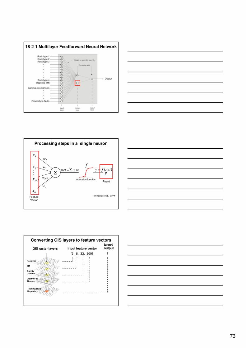
18-2-1 Multilayer Feedforward Neural Network
Processing steps in a single neuron
from Hassoun, 1995
geology(1-of-n coded) magnetic anomalygamma-ray
channelsto tal countdistance to nearest faultK
ThU
input layerhiddenlayer
internal biases =
x1
x2
xn-1
xn
w1
w2
wn-1
wn
y0
1
net =Σ x w y = f (net)f
Activation function
Feature Vector
Result
Converting GIS layers to feature vectorstargetoutput
1
Input feature vector
[3, 8, 33, 800]
GIS raster layers
Rocktype
EM
Gravity
Gradient
Distance to
Thrusts
Training sites
Deposits
74
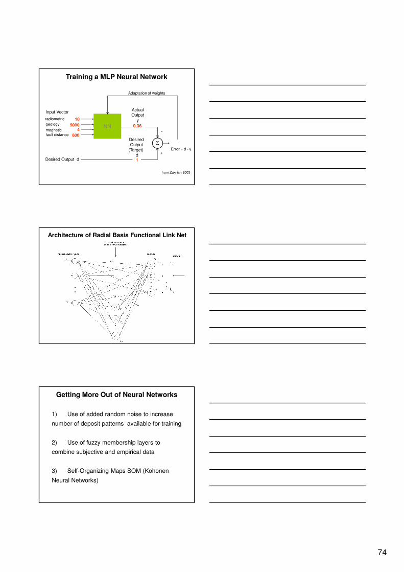
Desired Output d
Input Vector
geology
magneticfault distance
10
50004
600
ActualOutput
y
Training a MLP Neural Network
NN
Desired Output
(Target)
d1
0.36
Adaptation of weights
from Zaknich 2003
Error = d - y
Σ
-
+
radiometric
Architecture of Radial Basis Functional Link Net
1) Use of added random noise to increase
number of deposit patterns available for training
2) Use of fuzzy membership layers to
combine subjective and empirical data
3) Self-Organizing Maps SOM (Kohonen
Neural Networks)
Getting More Out of Neural Networks
75
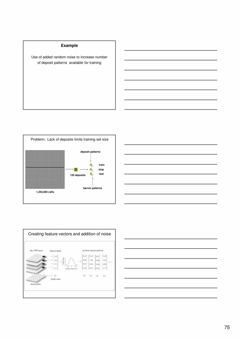
Use of added random noise to increase number
of deposit patterns available for training
Example
Problem: Lack of deposits limits training set size
1,254,000 cells
120 deposits
barren patterns
train
stop
test
deposit patterns
Creating feature vectors and addition of noise

76
Use of fuzzy membership layers to combine
subjective and empirical data
Example
Fuzzy-Neural Network Processing
Self-Organizing Maps SOM
(Kohonen Neural Networks)
Getting More Out of Neural Networks
77
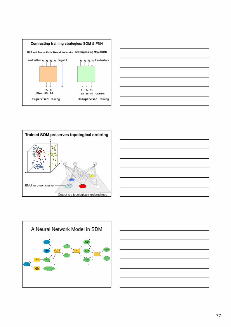
Contrasting training strategies: SOM & PNN
Self-Organizing Map (SOM)MLP and Probabilistic Neural Networks
Supervised Training Unsupervised Training
target, t
y1
x1 x2 x3 x4
y2
x1 x2 x3 x4
y1 y2 y3
Class 0.3 0.7 Clusterson off off
Input pattern Input pattern
Trained SOM preserves topological ordering
Output is a topologically ordered map
BMU for green cluster
y
x
z
yx Z
A Neural Network Model in SDM

78
Considerations for Neural Networks in SDM
• Training sites are point shapefiles used to train the neural network.
• There must be two training site shapefiles, Deposits and “Not” Deposits.
• For RBFLN and PNN, the training points are examples of
what is desired and not desired.
– Can assign fuzzy memberships to these sites.
– RBFLN sensitive to “Nots”
– PNN insensitive to “Nots”.
WHY USE NEURAL NETWORKS?WHY USE NEURAL NETWORKS?
uncertain, noisy data
outliers
non-linear relationships
multiple interdependent parameters
multiple populations
mixed data sets
� ratio, interval, ordinal nominal scales of data
measurements
Neural network techniques can deal with:
TYPES OF NEURAL NETWORKTYPES OF NEURAL NETWORK
•• SupervisedSupervisedRequires known deposit and nonRequires known deposit and non--deposit deposit
sites for trainingsites for training
Probabilistic Neural Networks (PNN)Probabilistic Neural Networks (PNN)
Radial Basis Functional Link Net (RBFLN)Radial Basis Functional Link Net (RBFLN)
•• UnsupervisedUnsupervisedAlgorithms that can find the natural Algorithms that can find the natural clustering within the dataclustering within the data
Self Organising Maps (SOM)Self Organising Maps (SOM)•• Trains on complete dataTrains on complete data
Fuzzy Neural Nets (FNN)Fuzzy Neural Nets (FNN)•• Trains on a random sample of dataTrains on a random sample of data

79
Demo 8Neural Network
How to Setup and Run a Neural Network using SDM in ArcGIS
Demo 81. Start Arcmap and open the Map Document c:\HY2010\MapDocuments\Lab8
2. Edit NN Tool 1 in the LabTools Toolbox and examine the inputs.
3. Run Neural Network Input Files tool. Notice that Model Builder will first runCombine and Band Collection Statistics tools.
4. Run GeoExplorer
5. Run RBFLN in GeoExplorer and follow the instructions given
6. When RBFLN has been completed EXIT GeoExplorer
7. Edit NN Tool 1 output files in the LabTool Toolbox. Run the entire model. The resulting grid should appear on map. Examine the results.
Demo 88. Edit NN Tool 2 in the LabTools Toolbox and examine the inputs. The difference
with the previous NN Tool 1 is that here we use two set of random points as ”training” and ”not training” sites and we will perfor a Fuzzy Clustering NN.
9. Run Neural Network Input Files tool. Notice that Model Builder will first runCombine and Band Collection Statistics tools.
10. Run GeoExplorer
11. Run Fuzzy Clustering in GeoExplorer and follow the instructions given
12. When Fuzzy Clustering has been completed EXIT GeoExplorer
13. Edit NN Tool 2 output files in the LabTool Toolbox. Run the entire model. The resulting grid should appear on map. Examine the results.
14. Compare visually the two NN models.

80
Table 1: Layers used in this Exercise
Layers are located in C:\HY2010\Derived\Fuzzy
Layer name Description
rc_till_cu Interpolated (IDW) surface of Cu
rc_till_as Interpolated (IDW) surface of As
rc_dnsstruli Density of faults
rc_lithodiv Lithodiversity
rc_amres2
Residual grid after subtracting median value
over 4 km radius neighborhood of airborne
magnetics
Comparison and Validation
Model Testing
Measures to compare, describe, and validate models
Simple Carlin Model Example
Measures of Models
• Correlation measures to compare models– Kappa for ranked models
– Pearson’s for raw models
• Fragstats: Measure the texture or appearance of the model. Does the model look geologic?
• Efficiency of Classification– Training sites
– Not-Training sites: What should “Nots” be?
• Efficiency of Prediction (Validation)– Sites not used for training
• ROC curves
• Jack-knife
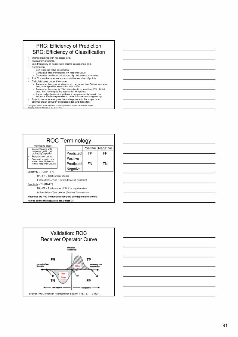
81
PRC: Efficiency of Prediction
SRC: Efficiency of Classification• Intersect points with response grid.
• Frequency of points.• Join frequency of points with counts in response grid.
• Summation– Sort response value descending
– Cumulative area from high to low response value.– Cumulative number of points from high to low response value.
• Plot Cumulative area versus cumulative number of points
• Calculate area under the curve.– Area under the curve for sites should be greater than 50% of total area,
then have a positive association with points.
– Area under the curve for “Not” sites should be less than 50% of total area, then have a positive association with points
– If area under the curve, then have a random association with the evidence. Evidence provides no better information than guessing.
• Point in curve where goes from steep slope to flat slope is an optimal break between predicted sites and not sites.
Chung and Fabbri, 2003, Validation of spatial prediction models for landslide hazard
mapping: Natural Hazards, v. 20, p.451-472
ROC Terminology
• Intersect points with response grid to get probability at points.
• Frequency of points.
• Summations with data sorted from highest to lowest response values.
Positive Negative
Predicted
Positive
TP FP
Predicted
Negative
FN TN
Sensitivity = TP/(TP + FN)
TP + FN = Total number of sites
1- Sensitivity = Type II errors (Errors of Omission)
Specificity = TN/(TN+FP)
TN + FP = Total number of “Not” or negative sites
1- Specificity = Type I errors (Errors of Commission)
Measures are free from prevalence (rare events) and thresholds.
How to define the negative sites (“Nots”)?
Processing Steps
Validation: ROC
Receiver Operator Curve
Brismar, 1991, American Roentgen Ray Society: v 157, p. 1119-1121.
Sites
“Not”
Sites
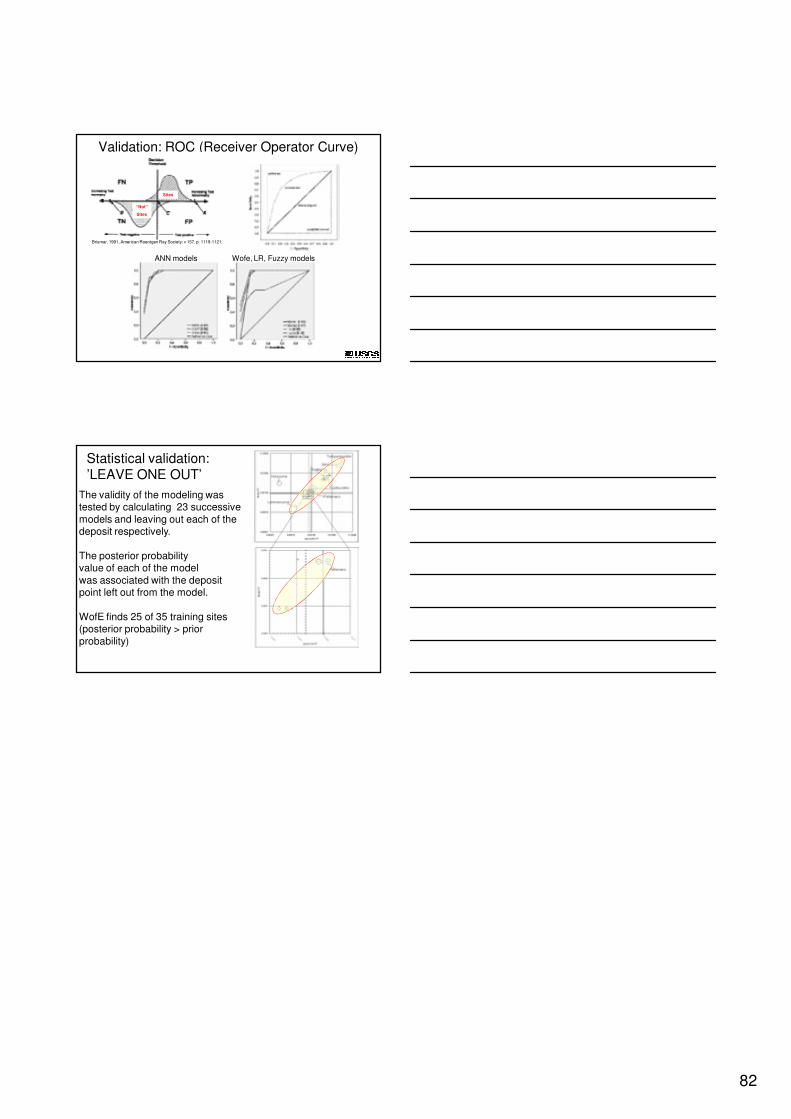
82
Validation: ROC (Receiver Operator Curve)
Brismar, 1991, American Roentgen Ray Society: v 157, p. 1119-1121.
Sites
“Not”
Sites
ANN models Wofe, LR, Fuzzy models
Statistical validation: ’LEAVE ONE OUT’
The validity of the modeling was tested by calculating 23 successive
models and leaving out each of thedeposit respectively.
The posterior probabilityvalue of each of the model
was associated with the depositpoint left out from the model.
WofE finds 25 of 35 training sites(posterior probability > prior
probability)


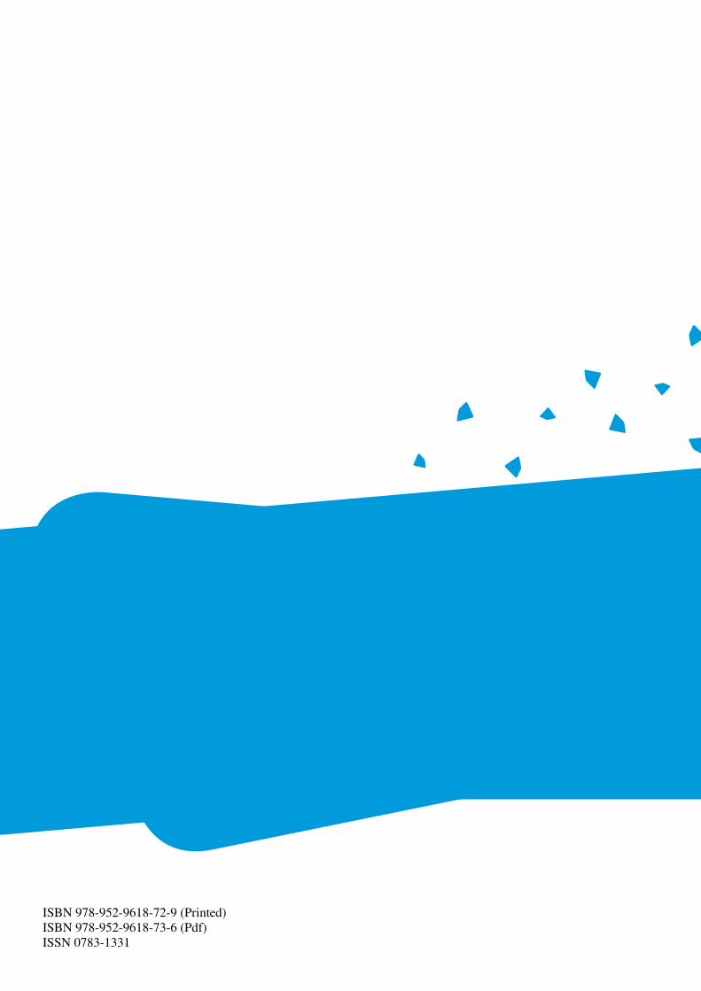
ISBN 978-952-9618-72-9 (Printed) ISBN 978-952-9618-73-6 (Pdf)ISSN 0783-1331


![Reactive transport of trace elements and isotopes in …webhome.auburn.edu/~leeming/lee-pub5.pdf[1] We integrate groundwater geochemistry, mineralogy, and numerical modeling techniques](https://img.pdfslide.us/doc/110x75/5fab3e56a69c6e545b4947f4/reactive-transport-of-trace-elements-and-isotopes-in-leeminglee-pub5pdf-1-we.jpg)