Embed Size (px)
Citation preview
PROSPECT THEORY AND ASSET PRICES
Nicholas Barberis
Ming Huang
Tano Santos
Course: Financial Economics, Ales Marsal, Presentation of the paper:
Outline
Game The story Assumptions What makes the paper different Model Intuition Numerical Results
Game
You were granted by 50 mil. Ales dollars (50 forints)
Ales mutual fund, probability 0.5 -> 20% growth; 0.5-> -20%
50% tax on holding cash, you invest = exempt of tax
YOU CAN WIN UP TO 125 mil A. dollars!!!
The Story
In consumption based models C=D, not in the data, investors have non-dividend income
Investors derives direct utility from consumption and financial wealth (concern about financial wealth fluctuation
The point of the game was: 1) to show that investors may or may not? be more sensitive to reductions in financial wealth than to increase, 2) after prior gains less loss averse
Introduction of changing risk aversion
The story
After a fall in stock prices, investor becomes more wary of further losses->more risk averse
Idea comes from prospect theory from psychology (i.e. evidence: subjects are offered a sequence of gambles, after gain people appear to be more risk seeking than usual, taking bets normally not accepted, ‘house money’ effect; TV show Card Sharks)
one explanation is that gains cushion the subsequent loss and losses are more painful than usual following prior losses vs. break even effect
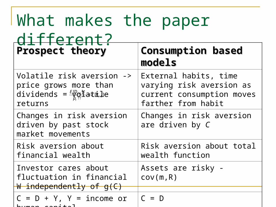
What makes the paper different?Prospect theoryProspect theory Consumption based Consumption based
modelsmodelsVolatile risk aversion -> price grows more than dividends = volatile returns
External habits, time varying risk aversion as current consumption moves farther from habit
Changes in risk aversion driven by past stock market movements
Changes in risk aversion are driven by C
Risk aversion about financial wealth
Risk aversion about total wealth function
Investor cares about fluctuation in financial W independently of g(C)
Assets are risky - cov(m,R)
C = D + Y, Y = income or human capital…
C = D
][][
11
t
t
t REp
DE
Assumptions
Continuum of identical infinitely lived agents One risky asset and one risk free asset
paying Rf,t+1, Rt+1
Risky asset is claim to a stream of perishable output represented by dividend sequence
Agents choose C and allocation to the risky asset
No large selling out
Model
]2......[)log(
]1......[)],,(1
(
11
11
1
0
tDDt
t
tttt
t
t
t
t
gD
D
zSXbC
E
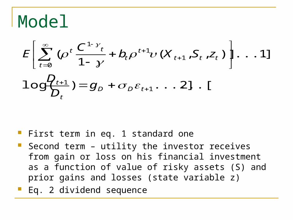
First term in eq. 1 standard one Second term – utility the investor receives from gain or loss
on his financial investment as a function of value of risky assets (S) and prior gains and losses (state variable z)
Eq. 2 dividend sequence
Model
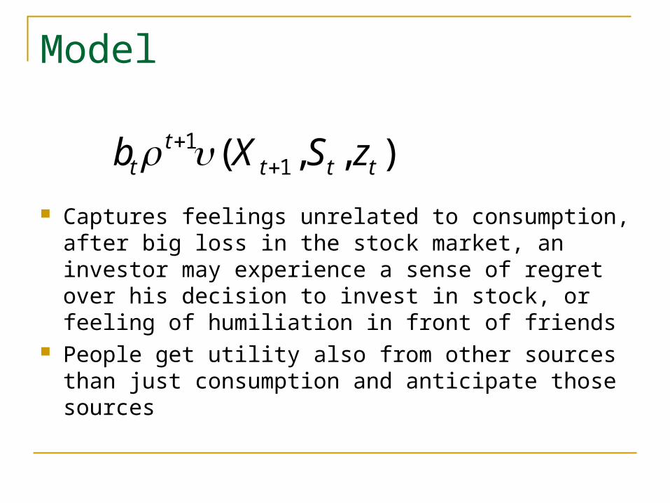
Captures feelings unrelated to consumption, after big loss in the stock market, an investor may experience a sense of regret over his decision to invest in stock, or feeling of humiliation in front of friends
People get utility also from other sources than just consumption and anticipate those sources
),,( 11
tttt
t zSXb
Model - gains and losses
Model – gains and losses
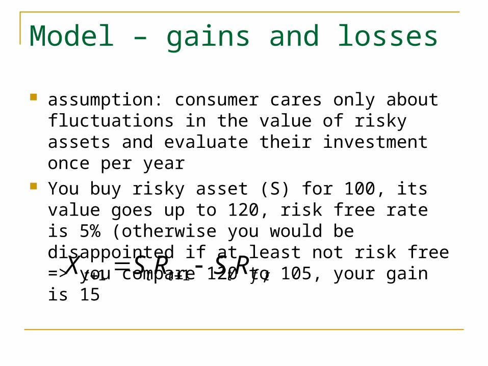
assumption: consumer cares only about fluctuations in the value of risky assets and evaluate their investment once per year
You buy risky asset (S) for 100, its value goes up to 120, risk free rate is 5% (otherwise you would be disappointed if at least not risk free => you compare 120 to 105, your gain is 15
tftttt RSRSX ,11
The model – prior outcomes
The model – prior outcomes
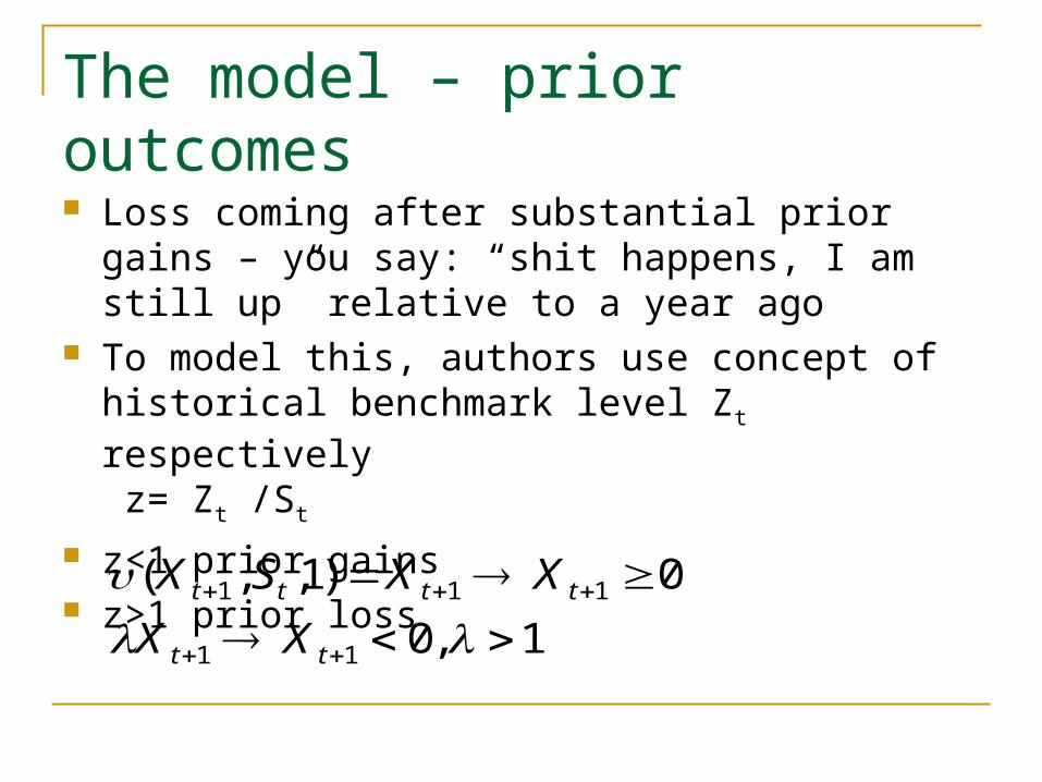
Loss coming after substantial prior gains – you say: “shit happens, I am still up” relative to a year ago
To model this, authors use concept of historical benchmark level Zt respectively z= Zt /St
z<1 prior gains z>1 prior loss
1,0
0)1,,(
11
111
tt
tttt
XX
XXSX
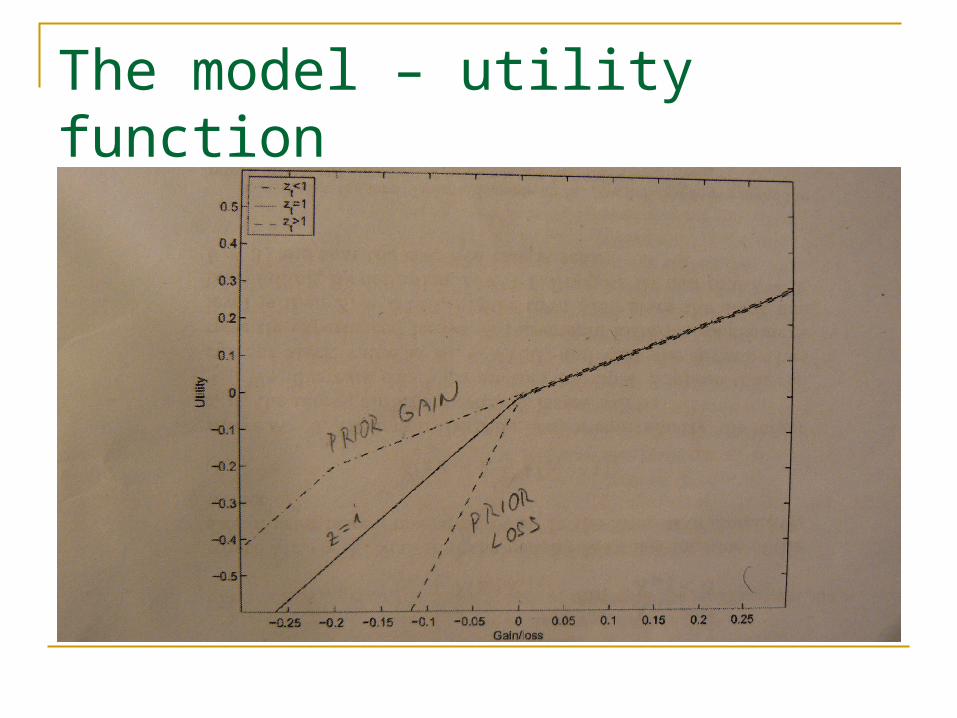
The model – utility function
The model – utility function
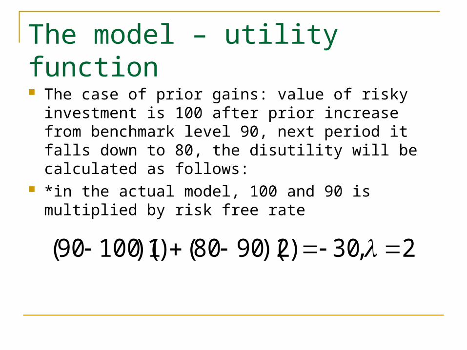
The case of prior gains: value of risky investment is 100 after prior increase from benchmark level 90, next period it falls down to 80, the disutility will be calculated as follows:
*in the actual model, 100 and 90 is multiplied by risk free rate
2,30)2)(9080()1)(10090(
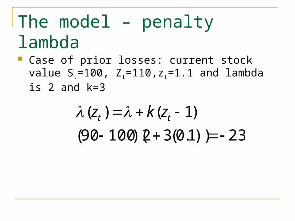
The model – penalty lambda
Case of prior losses: current stock value St=100, Zt=110,zt=1.1 and lambda is 2 and k=3
23))1.0(32)(10090(
)1()(
tt zkz
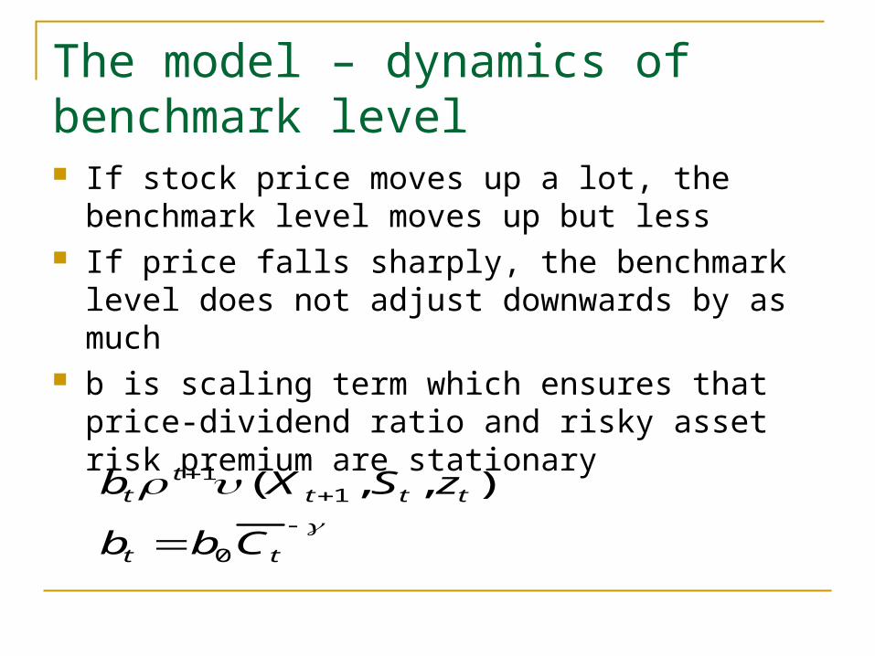
The model – dynamics of benchmark level If stock price moves up a lot, the benchmark level
moves up but less If price falls sharply, the benchmark level does
not adjust downwards by as much b is scaling term which ensures that price-
dividend ratio and risky asset risk premium are stationary
tt
tttt
t
Cbb
zSXb
0
11 ),,(
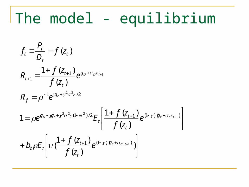
The model - equilibrium
))(
)(1(
)(
)(11
)(
)(1
)(
))(1(10
))(1(12/)1(
2/1
11
1
1222
22
1
tcc
tccccD
cc
tDD
g
t
tt
g
t
tt
gg
gf
g
t
tt
tt
tt
ezf
zfEb
ezf
zfEe
eR
ezf
zfR
zfD
Pf
How the model works
Ability of model to generate returns that are more volatile than dividends: high positive dividend innovation in the period->generate a high stock return->less risk averse investor ->he discounts the future dividend stream at a lower rate=>more volatile prices
This fact also generate predictability in long horizon: growing prices->growing price-dividend ration->lower returns, inverse relationship between future returns and price-dividend = Fama and French (1988)
Volatile stocks = substantial equity premium (investor is loss averse and fears frequent drop)
Low correlation of dividends and consumption
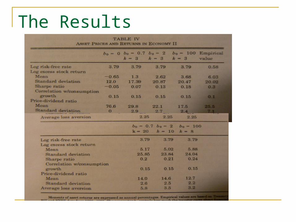
The Results
The Results
K determines how much more painful losses are when they come on the heels of other losses, k=3 makes the investor average loss aversion close to 2.25 which is based on micro data
b determines the relative importance of the prospect utility, no data->range
Increase in dividend volatility makes stocks more volatile, scaring the investor, although stocks are less correlated with consumption than in consumption based model, it does not matter since the investor cares about fluctuations in stock market per se