Embed Size (px)
Citation preview

Prosody Modeling in Concept-to-Speech
Generation
Shimei Pan
Submitted in partial fulfillment of the
requirements for the degree
of Doctor of Philosophy
in the Graduate School of Arts and Sciences
COLUMBIA UNIVERSITY
2002

c©2002
Shimei Pan
All Rights Reserved

Abstract
Prosody Modeling in Concept-to-Speech
Generation
Shimei Pan
With the development of speech recognition and synthesis technology, speech in-
terfaces for practical applications are in high demand. For applications like spoken
dialogues systems, where not only the waveform but also the content of a system’s
query/response have to be generated automatically, a Concept-to-Speech system
is needed. One key module in a Concept-to-Speech system is prosody modeling.
It determines how prosody (intonation), the suprasegmental aspect of speech that
communicates the structure and meaning of utterances, should be represented and
generated automatically. Since prosody directly affected by the meaning and struc-
ture of the sentences automatically produced by a natural language generator; at
the same time, it also has significant influence on the naturalness and effectiveness
of the speech synthesized, its performance is critical to the success of a Concept-
to-Speech system where both natural language generation and speech synthesis are
used together to generate the final spoken output.

In this thesis, I focus on two aspects of the prosody modeling process. First,
I explore novel features that are available during natural language generation, such
as the meaning, structure, and context of sentences, and demonstrate how these
features are related to prosody, based on empirical evidences derived from anno-
tated speech corpora. Second, I propose a new prosody modeling approach that
automatically combines different natural language features for prosody prediction.
More specifically, I designed an augmented instance-based learning algorithm that
makes use of the natural prosody in human speech to produce natural and vivid
synthesized speech. Our subjective evaluation demonstrates the effectiveness of
this approach. I implement the prosody modeling system for a medical application
called MAGIC.
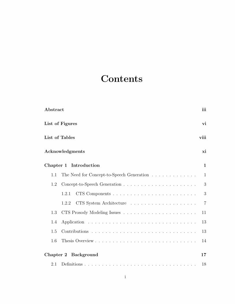
Contents
Abstract iii
List of Figures vi
List of Tables viii
Acknowledgments xi
Chapter 1 Introduction 1
1.1 The Need for Concept-to-Speech Generation . . . . . . . . . . . . . 1
1.2 Concept-to-Speech Generation . . . . . . . . . . . . . . . . . . . . . 3
1.2.1 CTS Components . . . . . . . . . . . . . . . . . . . . . . . . 3
1.2.2 CTS System Architecture . . . . . . . . . . . . . . . . . . . 7
1.3 CTS Prosody Modeling Issues . . . . . . . . . . . . . . . . . . . . . 11
1.4 Application . . . . . . . . . . . . . . . . . . . . . . . . . . . . . . . 13
1.5 Contributions . . . . . . . . . . . . . . . . . . . . . . . . . . . . . . 13
1.6 Thesis Overview . . . . . . . . . . . . . . . . . . . . . . . . . . . . . 14
Chapter 2 Background 17
2.1 Definitions . . . . . . . . . . . . . . . . . . . . . . . . . . . . . . . . 18
i

2.2 Prosody Theories and ToBI . . . . . . . . . . . . . . . . . . . . . . 20
2.3 Prosody and its Correlated Language Features . . . . . . . . . . . . 25
2.4 Natural Language Generation and Prosody . . . . . . . . . . . . . . 35
2.5 CTS Prosody Modeling . . . . . . . . . . . . . . . . . . . . . . . . . 39
2.6 Summary . . . . . . . . . . . . . . . . . . . . . . . . . . . . . . . . 42
Chapter 3 Prosody Modeling: Overview 43
3.1 Introduction . . . . . . . . . . . . . . . . . . . . . . . . . . . . . . . 43
3.2 Main Prosody Modeling Issues . . . . . . . . . . . . . . . . . . . . . 44
3.2.1 Prosody Predicting Features . . . . . . . . . . . . . . . . . . 44
3.2.2 Prosody Prediction Approaches . . . . . . . . . . . . . . . . 47
3.2.3 Prosody Evaluation . . . . . . . . . . . . . . . . . . . . . . . 50
3.3 CTS Prosody Modeling Architecture . . . . . . . . . . . . . . . . . 53
3.4 Corpora . . . . . . . . . . . . . . . . . . . . . . . . . . . . . . . . . 55
3.5 Summary . . . . . . . . . . . . . . . . . . . . . . . . . . . . . . . . 59
Chapter 4 Modeling SURGE Features for Prosody Modeling 60
4.1 Feature Description . . . . . . . . . . . . . . . . . . . . . . . . . . . 63
4.1.1 Word Class . . . . . . . . . . . . . . . . . . . . . . . . . . . 63
4.1.2 Syntactic/Semantic Constituent Boundary and Length . . . 64
4.1.3 Syntactic Function . . . . . . . . . . . . . . . . . . . . . . . 70
4.1.4 Semantic Role . . . . . . . . . . . . . . . . . . . . . . . . . . 72
4.1.5 Word and Surface Position . . . . . . . . . . . . . . . . . . . 74
4.2 The Analysis . . . . . . . . . . . . . . . . . . . . . . . . . . . . . . 74
4.2.1 Correlation Analysis . . . . . . . . . . . . . . . . . . . . . . 76
ii

4.2.2 Learning Prosody Prediction Rules . . . . . . . . . . . . . . 78
4.2.3 Patterns learned by RIPPER . . . . . . . . . . . . . . . . . 80
4.3 Summary . . . . . . . . . . . . . . . . . . . . . . . . . . . . . . . . 82
Chapter 5 Deep Semantic and Discourse Features 84
5.1 Feature Description . . . . . . . . . . . . . . . . . . . . . . . . . . . 84
5.1.1 Semantic Type . . . . . . . . . . . . . . . . . . . . . . . . . 84
5.1.2 Given/New . . . . . . . . . . . . . . . . . . . . . . . . . . . 86
5.1.3 Semantic Abnormality . . . . . . . . . . . . . . . . . . . . . 87
5.2 Analysis . . . . . . . . . . . . . . . . . . . . . . . . . . . . . . . . . 87
5.2.1 Correlation Analysis for Given/new . . . . . . . . . . . . . . 88
5.2.2 RIPPER Analysis for Semantic Type and Given/New . . . . 88
5.2.3 Semantic Abnormality and Prosody . . . . . . . . . . . . . . 89
5.2.3.1 Prosodic Features . . . . . . . . . . . . . . . . . . . 90
5.3 Summary . . . . . . . . . . . . . . . . . . . . . . . . . . . . . . . . 94
Chapter 6 Modeling Features Statistically for Prosody Prediction 95
6.1 Word Informativeness . . . . . . . . . . . . . . . . . . . . . . . . . . 96
6.1.1 Definitions of IC and TF*IDF . . . . . . . . . . . . . . . . . 98
6.1.2 Experiments . . . . . . . . . . . . . . . . . . . . . . . . . . . 100
6.1.2.1 Ranking Word Informativeness in the Corpus . . . 100
6.1.2.2 Testing the Correlation of Informativeness and Ac-
cent Prediction . . . . . . . . . . . . . . . . . . . . 102
6.1.2.3 Learning IC and TF*IDF Accent Models . . . . . . 102
6.1.2.4 Incorporating IC in Reference Accent Models . . . 104
iii

6.1.3 Summary and Discussion . . . . . . . . . . . . . . . . . . . . 107
6.2 Word Predictability . . . . . . . . . . . . . . . . . . . . . . . . . . . 109
6.2.1 Motivation . . . . . . . . . . . . . . . . . . . . . . . . . . . . 109
6.2.2 Word predictability Measures . . . . . . . . . . . . . . . . . 111
6.2.2.1 N-gram Predictability . . . . . . . . . . . . . . . . 112
6.2.2.2 Mutual Information . . . . . . . . . . . . . . . . . 113
6.2.2.3 The Dice Coefficient . . . . . . . . . . . . . . . . . 114
6.2.3 Statistical Analyses . . . . . . . . . . . . . . . . . . . . . . . 116
6.2.4 Word Bigram Predictability and Accent . . . . . . . . . . . 118
6.2.5 Learning Accent Prediction Models . . . . . . . . . . . . . . 119
6.2.6 Relative Predictability . . . . . . . . . . . . . . . . . . . . . 121
6.2.7 Summary . . . . . . . . . . . . . . . . . . . . . . . . . . . . 122
6.3 Word Informativeness and Word Predictability . . . . . . . . . . . . 123
Chapter 7 Combining Language Features in Prosody Prediction 124
7.1 A Comparison of Rule-based and Instance-based Approach . . . . . 126
7.1.1 Generalized Rule Induction . . . . . . . . . . . . . . . . . . 126
7.1.2 Instance-based Prosody Modeling . . . . . . . . . . . . . . . 127
7.2 RIPPER-based Prosody Modeling . . . . . . . . . . . . . . . . . . . 129
7.3 Instance-based Prosody Prediction . . . . . . . . . . . . . . . . . . 133
7.3.1 Introduction . . . . . . . . . . . . . . . . . . . . . . . . . . . 133
7.3.2 Instance-based learning: an Extension . . . . . . . . . . . . 135
7.3.2.1 Parameters in Viterbi-based Beam Search . . . . . 136
7.3.2.2 The Viterbi Algorithm . . . . . . . . . . . . . . . . 138
7.3.3 Prosody Modeling Using Instance-based Learning . . . . . . 139
iv

7.3.3.1 Signature Feature Vector: a Training Instance . . . 140
7.3.3.2 Target Cost and Transition Cost . . . . . . . . . . 142
7.3.3.3 The Viterbi Algorithm . . . . . . . . . . . . . . . . 146
7.4 Evaluating Instance-based Prosody Modeling . . . . . . . . . . . . . 148
7.5 TTS versus CTS . . . . . . . . . . . . . . . . . . . . . . . . . . . . 153
7.6 Summary . . . . . . . . . . . . . . . . . . . . . . . . . . . . . . . . 157
Chapter 8 Conclusions and Future Work 158
8.1 Summary of Approach . . . . . . . . . . . . . . . . . . . . . . . . . 158
8.2 Summary of Contributions . . . . . . . . . . . . . . . . . . . . . . . 161
8.3 Summary of Limitations and Future Work . . . . . . . . . . . . . . 164
Appendix A 167
v

List of Figures
1.1 Main CTS Modules . . . . . . . . . . . . . . . . . . . . . . . . . . . 4
1.2 Traditional CTS Architecture . . . . . . . . . . . . . . . . . . . . . 7
1.3 The New CTS Architecture . . . . . . . . . . . . . . . . . . . . . . 11
2.1 Pierrehumbert’s Intonation Grammar . . . . . . . . . . . . . . . . . 21
2.2 A RST Representation of a Discourse Segment . . . . . . . . . . . . 36
2.3 A Systemic Representation Used in SURGE . . . . . . . . . . . . . 38
2.4 The Input Representation of RealPro . . . . . . . . . . . . . . . . . 38
3.1 Prosody Modeling Architecture . . . . . . . . . . . . . . . . . . . . 53
3.2 A Segment of the Spontaneous Speech Corpus . . . . . . . . . . . . 56
3.3 A Segment of the Read Speech Corpus . . . . . . . . . . . . . . . . 56
3.4 A Segment of the Text Corpus . . . . . . . . . . . . . . . . . . . . . 58
4.1 A Simplified Final FD . . . . . . . . . . . . . . . . . . . . . . . . . 62
4.2 The Category Information in an FD . . . . . . . . . . . . . . . . . . 64
4.3 The Syntactic/Semantic Constituent Boundaries . . . . . . . . . . . 65
4.4 Syntactic Functions in an FD . . . . . . . . . . . . . . . . . . . . . 70
4.5 A Hierarchical Representation of Syntactic Function . . . . . . . . . 71
vi

4.6 The Semantic Roles in an FD . . . . . . . . . . . . . . . . . . . . . 72
4.7 The Semantic Role information in an FD . . . . . . . . . . . . . . . 73
5.1 A Segment of the MAGIC Ontology . . . . . . . . . . . . . . . . . . 85
7.1 The Viterbi Algorithm . . . . . . . . . . . . . . . . . . . . . . . . . 139
7.2 An Example of a Viterbi Search Result . . . . . . . . . . . . . . . . 147
vii

List of Tables
3.1 A Segment of the Annotated Read Speech Corpus . . . . . . . . . . 57
3.2 A Segment of the Annotated Spontaneous Speech Corpus . . . . . . 58
4.1 Definitions for Different Syntactic/Semantic Constituent Boundaries 67
4.2 Precedence Among Syntactic/Semantic Constituent Boundaries . . 69
4.3 An Example of the Syntactic/Semantic Constituent Boundary and
Length Assignment . . . . . . . . . . . . . . . . . . . . . . . . . . . 70
4.4 Semantic Roles Extracted from an FD . . . . . . . . . . . . . . . . 74
4.5 Summary: The Correlations Between SURGE Features and Prosody 76
4.6 Summary: The Different Prediction Models Learned by RIPPER . 79
5.1 The Correlations between Given/new and Prosody . . . . . . . . . 88
5.2 Summary: The Different Prediction Models Learned by RIPPER . 89
5.3 Abnormality and Prosodic Features. . . . . . . . . . . . . . . . . . . 91
5.4 Abnormality and Index Difference. . . . . . . . . . . . . . . . . . . 94
6.1 IC Most and Least Informative Words . . . . . . . . . . . . . . . . 101
6.2 TF*IDF Most and Least Informative Words . . . . . . . . . . . . . 101
6.3 The Correlation of Informativeness and Accentuation . . . . . . . . 102
viii

6.4 Comparison of the IC, TF*IDF Models with the Baseline Model . . 103
6.5 Comparison of the POS+IC Model with the POS Model . . . . . . 105
6.6 Comparison of the TTS+IC Model with the TTS Model . . . . . . 105
6.7 Top Ten Most Collocated Words for Each Measure . . . . . . . . . 114
6.8 Correlation of Different Predictability Measures with Accent Decision 117
6.9 Bigram Predictability and Accent for cell Collocations . . . . . . . . 118
6.10 Ripper Results for Accent Status Prediction . . . . . . . . . . . . . 120
6.11 RIPPER Rules for the Combined Model . . . . . . . . . . . . . . . 121
6.12 Relative Predictability and Accent Status . . . . . . . . . . . . . . . 122
7.1 Ripper Results for the Combined Model . . . . . . . . . . . . . . . 130
7.2 The Combined Pitch Accent Prediction Model . . . . . . . . . . . . 131
7.3 The Combined Break Index (1) Prediction Model . . . . . . . . . . 131
7.4 The Combined Break Index (2) Prediction Model . . . . . . . . . . 132
7.5 The Feature Vector in the Speech Training Corpus . . . . . . . . . . 140
7.6 The Distance Vector for Weight Training . . . . . . . . . . . . . . . 144
7.7 Instance-based Prosody Modeling Performance . . . . . . . . . . . 148
7.8 Subjective Pair Evaluation . . . . . . . . . . . . . . . . . . . . . . . 152
7.9 TTS versus CTS . . . . . . . . . . . . . . . . . . . . . . . . . . . . 155
7.10 TTS versus CTS POS in Pitch Accent Prediction . . . . . . . . . . 155
7.11 TTS versus CTS in Break Index Prediction . . . . . . . . . . . . . . 156
A.1 Acronym Index . . . . . . . . . . . . . . . . . . . . . . . . . . . . . 168
ix

Dedication
This thesis is dedidated with gratitude and love to
Xuejun Bian
x

Acknowledgments
I would like to thank first my thesis advisors, Kathleen McKeown and Julia Hirschberg,
who provided invaluable direction and support throughout my thesis work. In par-
ticular, I want to thank Kathy for bringing me into the field of language and speech
generation; for her encouragement on even the smallest progress I made, for giving
me the freedom to explore prosody and speech research. I also want to thank Julia
for her insight, constructive criticism, and setting high standard for my work.
I want to thank the members of my thesis committee: Steven Feiner, Julia
Hirschberg, Judith Klavans, Kathleen McKeown, and Mari Ostendorf for their en-
couragements, insights, and feedbacks. I also want to thank Diane Litman from
whom I learned the basic knowledge on conducting empirical analysis.
I own many thanks to my colleagues and friends from Columbia. I was very
lucky to have three wonderful officemates and friends: Regina Barzilay, Noemie
Elhadad, and James Shaw. Among them, James is the kindest, Regina is the
warmest, and Noemie is the sweatest. I also want to thank two of my closest
friends, Hongyan Jing and Michelle Zhou. Their friendships help make my years in
Columbia enjoyable and memorable.
I thank my other colleagues in the natural language processing group, es-
xi

pecially Kris Concepcion, Liz Chen, and Min-Yen Kan who helped me record
some speech corpora; Regina Barzilay, David Evans, Melissa Holcombe, Min-Yen
Kan, Carl Sable, and Barry Schiffman who volunteered to be the subjects in my
study; Pablo Duboue, Pascale Fung, Vasileios Hatzivassiloglou, Becky Passonneau,
Dragomir Radev, and Jacques Robin for valuable discussions. I also want to thank
Desmond Jordan and Shabina Ahmad from the Columbia Presbyterian Medical
Center (CPMC) for their help in collecting and annotating medical corpora.
I want to thank my family for their unconditional love and support, especially
my parents Meijuan and Yaohua, my brother Nan, and my sister Yiqing. Without
their encouragements, I never could have begun, much less completed this thesis.
Finally, I would like to thank those institutions that supplied funding for this
research:DARPA Contract DAAL01-94-K-0119, and NSF grant IRI 9528998, Na-
tional Library of Medicine grants R01-LM06593-01 and LM06593-02, and Columbia
University Center for Advanced Technology in High Performance Computing and
Communications in Healthcare (funded by the New York State Science and Tech-
nology Foundation).
xii

1
Chapter 1
Introduction
1.1 The Need for Concept-to-Speech Generation
People have envisioned using speech to enable human-machine communication for
several decades. Recently, with the development of speech understanding and pro-
duction technology, speech interfaces for practical applications are commonplace.
For example, computer systems use voice interfaces for information services, includ-
ing providing airline ticket information, stock market information, and personal
banking or credit information. Some of these applications have brought financial
benefits for the businesses involved. At the same time, they also stimulate new
demands for better speech understanding and production technology. There is still
considerable room for further improvement for both speech understanding and pro-
duction. For example, the error rate for speech recognition in unrestricted domains
is frequently too high for spoken language systems to be used effectively, while the
intelligibility and naturalness of synthesized speech is not good enough to be widely
accepted by users. In this thesis, I will address several research issues in automatic

2
speech production.
Typical speech production systems can be divided into two types: Text-
to-Speech (TTS) systems and Concept-to-Speech (CTS) systems. For the past
decades, TTS has been the main research focus in speech production. In a TTS
system, spoken utterances are automatically produced from online text. For exam-
ple, a TTS system can be used to read email or news stories. However, for appli-
cations, such as spoken dialogue systems, where not only the sound but also the
content of a sentence has to be generated automatically, a CTS system is needed. A
CTS system takes concepts or semantic representations, such as database entities,
templates or logical forms, as input, and transforms them first into grammatical
sentences, and subsequently, into natural and coherent spoken utterances.
In recent years, CTS research has grown rapidly. More and more CTS appli-
cations have been developed for different applications and some of them have been
put into practical use, such as the Philips train timetable information system for
intercity trains in both Germany and Switzerland, Nuance’s Better Banking sys-
tem as well as its travel planning system, and Speechwork’s United Airline ticket
reservation system. CTS systems potentially may also be used to customize and
summarize sports, financial or weather information for drivers in moving vehicles.
More generally, CTS systems provide a natural communication channel for infor-
mation systems, allowing a hands-free and eyes-free environment.

3
1.2 Concept-to-Speech Generation
1.2.1 CTS Components
The task of transforming concepts into speech is difficult even for human beings.
For example, in public speaking, given a topic and raw materials, determining how
to communicate them clearly and smoothly is not a trivial task. In general, the
speaker has to decide what to include, find out the relations between different
materials, and decide how to organize them in a logical way. Once the content and
high level structuring are decided, she has to make more fine-grained decisions, such
as how to choose wording to make the presentation clear. She may also need to
rehearse several times to make sure that the main points are highlighted, the pace is
appropriate, and the rhythm is pleasant. Speaking in a conversational environment
may require less preparation. However, a speaker still has to decide what to say,
and how to say it in a natural, coherent, and clear fashion.
Systematically developing a Concept-to-Speech system to automatically trans-
form concepts into speech is a complicated process. As in human spoken language
production, a CTS system also has to make decisions on the content, the structur-
ing of the content, the wording, the pronunciation, and the rhythm of speech. In
order to facilitate CTS development, a full-fledged CTS system can be partitioned
into five main modules: a content planner, a sentence planner, a surface realizer, a
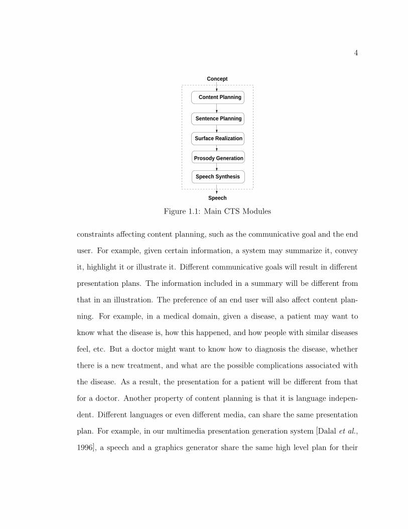
prosody generator, and a speech synthesizer. Figure 1.1 shown these CTS modules
in a pipeline.
A content planner decides what information needs to be communicated as
well as the high level structuring of the conveyed information. There are many
4
Speech
Prosody Generation
Speech Synthesis
Content Planning
Sentence Planning
Surface Realization
Concept
Figure 1.1: Main CTS Modules
constraints affecting content planning, such as the communicative goal and the end
user. For example, given certain information, a system may summarize it, convey
it, highlight it or illustrate it. Different communicative goals will result in different
presentation plans. The information included in a summary will be different from
that in an illustration. The preference of an end user will also affect content plan-
ning. For example, in a medical domain, given a disease, a patient may want to
know what the disease is, how this happened, and how people with similar diseases
feel, etc. But a doctor might want to know how to diagnosis the disease, whether
there is a new treatment, and what are the possible complications associated with
the disease. As a result, the presentation for a patient will be different from that
for a doctor. Another property of content planning is that it is language indepen-
dent. Different languages or even different media, can share the same presentation
plan. For example, in our multimedia presentation generation system [Dalal et al.,
1996], a speech and a graphics generator share the same high level plan for their

5
presentation. After content planning, the intermediate representation may include
discourse structure and discourse relations.
Unlike content planning, which is mostly language independent, a sentence
planner decides how to use appropriate semantic structure and wording to com-
municate input concepts. Therefore, it relies mostly on linguistic knowledge, such
as grammatical and lexical knowledge. Since a sentence planner primarily uses
linguistic knowledge, it can be done in a more domain independent fashion.
In sentence planning, based on the meanings of, and the relations between,
input concepts, a system may first assign appropriate semantic roles for each input
concept, and then the semantic structure of a sentence can be constructed. Once the
semantic structure is chosen, the system may consult a concept-indexed lexicon, and
decide which words, or phrases can best communicate the input concepts. Lexical
selection is primarily influenced by the input concepts, the discourse context, as
well as the end user. For example, if the end user is a doctor, the presentation may
include many abbreviations so that communication is concise. However, medical
terms and abbreviations can be difficult for a patient to understand if she does
not have medical knowledge. Therefore, if possible, the system should avoid using
abbreviations if the same information is presented to a patient.
Sentence planning is less domain-dependent than content planning. Never-
theless, due to its requirement for extensive linguistic knowledge as well as real
world knowledge, so far, no reusable sentence planner is currently available in the
public domain. After sentence planning, the intermediate representation may in-
clude semantic roles and semantic constituent structures.
A surface realizer uses an English grammar, transforming a lexicalized se-

6
mantic structure into a syntactic structure, linearizing the structure, and handling
morphology and function word generation. The features available after surface re-
alization may include syntactic constituent structure, syntactic function (subject,
object, complements etc.), and part-of-speech. Other information, such as the lex-
ical word, word position and distance, can be easily computed from a string of
words.
There are several surface realizers available in the public domain, such as
FUF/SURGE [Elhadad, 1993; Robin, 1994], KPML [Matthiessen and Bateman,
1991] and RealPro [Lavoie and Rambow, 1997]. Because of the availability of
these systems, a generation system developer can focus more on the application-
dependent part of the system for new applications.
In general, the same text can be spoken in many different ways: the speaking
rate can be higher or lower, words can be emphasized or de-emphasized, and extra
pauses can be inserted at different locations. These variations affect the meaning
of utterances and the ways in which listeners interpret them. These variations
are generated in a CTS system by the prosody modeling component. A prosody
modeling system makes decisions on the variations of a collection of speech features
relating to how sentences are spoken, such as pitch, loudness, tempo, and rhythm.
It is one of the major CTS components that affect the naturalness and intelligibility
of synthesized speech. In general, proper prosodic variations make speech sound
clear, easy to understand, and vivid. In contrast, inappropriate prosodic variations
make the speech unnatural, hard to understand, and sometimes even misleading.
Finally, a speech synthesizer takes the words in a sentence as well as their
prosodic assignments as input, and produces the synthesized speech signal. A

7
Text
Text Generation
Speech
Text−to−Speech
Sentence Planning
Surface Realization
Content Planning
Concept Speech Synthesis
Prosody Generation
Figure 1.2: Traditional CTS Architecture
speech synthesizer makes decisions on how to pronounce words in a given con-
text, how to generate a sequence of acoustic-phonetic units given its pronunciation,
how to realize the fundamental frequency contour, duration, and pauses given the
prosody assignments, and how to synthesize the final waveform. Right now, most
general-purpose speech synthesizers have been developed for TTS systems.
1.2.2 CTS System Architecture
Traditionally, CTS generation was done in two separate stages: text generation
or natural language generation (NLG), which includes the first three components,
and Text-to-Speech, which includes the last two components. In such a system, the
text generator first produces grammatical sentences from concepts, then a Text-to-
Speech synthesizer produces speech from the text. Most spoken dialogue systems,
such as TOOT [Litman et al., 1998; Litman and Pan, 1999], Elvis [Walker, 2000],
and the CMU communicator [Rudnicky et al., 1999], employ this architecture for
spoken language generation. As shown in Figure 1.2, the interface between the
text generator and the TTS system contains only text. This architecture has its

8
advantages. Both text generation and TTS have been studied for decades and there
are reusable components in both areas. Thus, in such a CTS system, in addition to
text generation and Text-to-Speech, no extra effort is required for NLG and TTS
integration. Although this architecture is simple and convenient, it suffers major
drawbacks, as described by Zue [Zue, 1997]:
“Currently, the language generation and text-to-speech components on the
output side of conversational systems are not closely coupled; the same text is gen-
erated whether it is to be read or spoken. Furthermore, current systems typically
expect the language generation component to produce a textual surface form of a sen-
tence (throwing away valuable linguistic and prosodic knowledge) and then require
the text-to-speech component to produce linguistic analysis anew. Clearly, these two
components would benefit from a shared knowledge base.”
In general, sentences need to be understood before they can be spoken prop-
erly. The TTS component needs to know the meaning and the structure of the text
before it can decide how to communicate them in speech. For example, discourse
context influences the accentual patterns of speech.
(1) Q: Who went to Columbia University?
A: MARY went to Columbia University.
(2) Q: Which University did Mary go to?
A: Mary went to COLUMBIA University.
In this example, depending on the question, the same answer may have different
accentual patterns. In the first example, since Mary is the focus, it gets emphasized.
In the second example, Columbia is the focus and it is emphasized instead. In order
to identify the focus of an utterance, the TTS component employed by such a CTS

9
system has to conduct text analysis, such as discourse, semantic, and syntactic
analysis. With existing text understanding technology, however, these tasks are
extremely difficult, if not impossible. As a result, some information that is critical
for speech synthesis is missing in such an uncoupled CTS system. The inability to
recover useful information in TTS is one of the main problems this type of CTS
system suffers.
In a CTS system, sentences are automatically generated from deep discourse,
semantic, and syntactic representations, and thus, theoretically, a CTS system is
able to accurately realize the underlying intention and meaning of a generated
sentence. Thus, no text analysis is necessary if the integration is done properly. In
order to make this information available for speech synthesis, the interface between
text generation and speech synthesis should include not only the text but also the
associated discourse, semantic, and syntactic information. This requires a richer
and more structured representation for the integration interface.
Overall, there are two major concerns in CTS integration: usability and
reusability. On the one hand, the structured linguistic data has to be represented
in the interfaces so that it is usable during speech synthesis. On the other hand,
in both language generation and speech synthesis, there are some reusable compo-
nents. The main concern for reusability is to leverage existing technology so that
new CTS systems do not need to be designed from scratch.
In terms of reusability, the text-based uncoupled CTS architecture is the
highest because of its ability to effectively reuse existing natural language generation
and TTS components. It, however, scores the lowest in the usability measure
because much useful structural information is missing in speech synthesis, which

10
leads to low synthesis quality.
In this thesis, I propose a CTS architecture, shown in Figure 1.3 which has
both high usability and reusability. On the one hand, it can effectively reuse existing
natural language generation and speech synthesis technology. On the other hand,
the structural information produced by the natural language generator is kept in
the interface and therefore, is available for speech synthesis. In [Pan and McKeown,
1997], we proposed a Speech Integration Markup Language (SIML) to represent the
interface between text generation and speech synthesis. This markup language can
represent not only the text, but also discourse, semantic, and syntactic structures.
Further more, since the definition of the markup language follows the Standard
Generalized Markup Language (SGML) specifications, it makes the integration of
different CTS components easier.
In addition, for CTS systems, the production of natural, intelligible speech
depends in part on the production of proper prosody, variations in pitch, tempo, and
rhythm. Prosody modeling depends on associating variations of prosodic features
with changes in structure, meaning, intent, and context of the language spoken.
For CTS systems employing the proposed architecture, such information is readily
available when language is produced from concepts and a prosody modeling com-
ponent needs to be designed specifically to take advantage of the availability of this
information. Since prosody modeling is one of the main research foci in the thesis,
in the following, I briefly describe some of the research issues in designing a prosody
modeling component for CTS generation.

11
Prosody
Text
Text Generation
SpeechSynthesis
ProsodyModeling
Speech
Learning
Text
Prosody GenerationStructures
Training MachineCorpora
Content Planning
Concept
Surface Realization
Sentence Planning
Figure 1.3: The New CTS Architecture
1.3 CTS Prosody Modeling Issues
Prosody modeling decides what and how features produced by a natural language
generator affect prosodic variations. Since the performance of prosody modeling
is critical to speech synthesis quality, whether a prosody modeling component can
effectively make use of information produced during language generation is vital
for the performance of a Concept-to-Speech system.
Prosody modeling is a complex process. For example, prosody is inextricably
linked to many discourse, semantic, and syntactic features. At the same time, not
all discourse, semantic, and syntactic features affect prosody. As a result, how to
identify useful natural language features for prosody prediction is one of the main
foci in prosody modeling.
Unlike the features generated by a natural language generator, which are
well-defined given a natural language generator, there are also features, such as the
semantic weight of a word, that are not directly represented in typical text gener-
ation systems. However, their usefulness in prosody modeling has been suggested
in the literature. In order to investigate their influence on prosody modeling, one

12
of the research foci in this research is to first systematically model these features,
and then empirically verify their usefulness in prosody prediction.
Prosody itself is a very complicated phenomenon. It correlates with many
acoustic features, such as pitch, intensity, duration, speaking rate, and pause. How
to represent these features in a systematic and meaningful way is also a main
research issue in prosody modeling. In the thesis, a standard prosody annotation
framework for American English, the ToBI prosody labeling convention, is used as
the representation scheme of prosodic features. A detailed description of the ToBI
convention is given in Chapter 2.
In addition to the issues in identifying and representing natural language and
prosodic features, how to build a computational model to predict prosodic features
based on natural language features is another important research issue. Predicting
prosodic variations is hard due to the interactions among language features as well
as the interactions among prosodic features. In natural speech, several prosodic
decisions may be made simultaneously and the decision on one prosodic feature
may affect the decision on another. For example, where to put the main stress of a
sentence may be affected by prosodic phrasing as well as the accentual patterns of
adjacent words. Thus, how to take care of the interactions among different language
and prosodic features in prosody modeling is another important research issue to
be addressed in prosody modeling.
Once a prosody modeling system is built, it is also important to know
whether one system is better than another so that the improvement of a new sys-
tem can be measured. Therefore, system evaluation is a critical topic in prosody
modeling.
13
In summary, when building a prosody modeling system, four basic issues
need to be resolved: natural language feature identification and modeling, prosodic
feature representation, prosodic feature prediction, and system evaluation. Because
ToBI is adopted for prosodic feature representation, the main foci of this study are
the remaining three topics.
1.4 Application
The CTS system developed in this study was tested as part of MAGIC, a multi-
media presentation generation system for cardiac intensive care [Dalal et al., 1996].
MAGIC is able to produce a coordinated speech and graphics presentation on a pa-
tient’s post-operative status, using the patient’s record in a large medical database.
The patient’s record includes critical events that occur during a bypass operation,
vital signs, medical history, related lab results, and treatment received. Typically,
the semantics of and the relationships between database entities are unambiguously
defined when the database is created. Given this information as input, the CTS
generator of MAGIC automatically produces briefings on a patient’s post-bypass
status in spoken language.
1.5 Contributions
The main contribution of this thesis is on automatic prosody modeling for Concept-
to-Speech generation. More specifically,
1. I systematically identify and model a wide range of natural language features
available in CTS for prosody prediction. Through this investigation, I iden-

14
tify a few new features, such as word informativeness, word predictability,
and syntactic function, that are useful for prosody modeling. Some of these
features have not been empirically verified before and have not been incorpo-
rated in existing prosody modeling systems.
2. I design an instance-based prosody modeling algorithm that has better perfor-
mance than existing generalization-based prosody modeling approaches. Based
on a set of pre-annotated training instances, this new approach can be used to
systematically combine language features from a stream of words and predicts
all the prosodic features associated with all the words simultaneously.
3. The CTS prosody modeling system proposed has been implemented and tested
for MAGIC, a multimedia presentation generation system for intensive care.
MAGIC provides not only a context for this investigation but also a platform
for testing and verifying the adequacy and significance of the proposed CTS
prosody modeling system when it is applied in a real world application.
Overall, the work presented in this thesis addresses several main issues in
Concept-to-Speech prosody modeling. This will impact both CTS system design
as well as CTS prosody modeling.
1.6 Thesis Overview
Chapter 2 provides essential background information of this work. It defines main
concepts used in the dissertation. It also reviews the most relevant theoretical
and empirical work in this area. The related work is documented in four parts:

15
intonation theories and the ToBI annotation standard, the relationship between
prosody and various linguistic features, typical text generation systems and existing
Concept-to-Speech systems.
Chapter 3 provides an overview of the prosody modeling architecture as
well as main research issues in prosody modeling. For each of the main issues, it
discusses its importance, possible solutions, the approach employed in the study,
and justifications for choosing this approach. A brief description of the speech and
text corpora used for this study is also included in this chapter.
Since prosody modeling is the main topic of the thesis, in addition to Chap-
ter 3, four more chapters are used to describe this process. Three of the four
chapters describe how to identify and model different features available in NLG
for prosody modeling. Chapter 4 focuses on the sentential features represented in
the SURGE surface realizer. Main features covered in this chapter include part-
of-speech, syntactic/semantic constituent boundary, syntactic/semantic constituent
length, syntactic functions, semantic roles, word, and surface position. Chapter 5 fo-
cuses on deep semantic and discourse features. Main features covered in the chapter
include semantic type, semantic abnormality, and discourse given/new. Chapter 6
focuses on the features that are not typically represented in a text-based natural
language generation system and therefore, must be statistically modeled using a
text corpus. Main features covered in this chapter include word informativeness
and word predictability.
In addition, Chapter 7 discusses an instance-based prosody modeling ap-
proach as well as experiments conducted for system evaluation.
Finally, Chapter 8 summarizes the thesis work and points out limitations as

16
well as future directions of this work.

17
Chapter 2
Background
In this chapter, I provide an overview of the theories and systems closely related
to the main research issues discussed in the dissertation. To facilitate the explana-
tion, in section 2.1, I first define terms used throughout the dissertation. Once the
meaning of each term is clarified, in section 2.2, I give an overview of the theoretical
background of prosody. Basically, the described intonation theories form the foun-
dation of the syntax and semantics of English intonation and ToBI is a practical
prosody labeling guideline that grew out of these theories. In addition, since identi-
fying and modeling language features produced by a natural language generator and
then predicting prosodic variations using these features are the main research foci
of the dissertation, the remainder of the related work section is organized around
these two topics. Section 2.3 describes typical language features that were previ-
ously found useful for prosody prediction. Section 2.4 describes the availability of
typical language features in natural language generation. Finally, since most au-
tomatic prosody modeling work described in the literature concentrates on TTS,
in section 2.5, I focus on prosody modeling in the context of Concept-to-Speech

18
generation.
2.1 Definitions
Since the dissertation is about Concept-to-Speech and prosody modeling, the first
two concepts to be introduced are Concept-to-Speech and prosody. A Concept-to-
Speech generator, also called Data-to-Speech, Message-to-Speech, and Meaning-to-
Speech generator, is a computational system that automatically produces spoken
language (including the content and the associated speech signals) from a semantic
representation. In Chapter 1, I explained that typical input to a Concept-to-Speech
system may include database entities, templates, and first-order predicates. The
main functions of a Concept-to-Speech system include selecting and organizing con-
tent, selecting words and sentence structures, generating grammatical sentences,
predicting prosodic variations, and synthesizing speech signals. Since prosody pre-
diction is one of the main tasks in CTS generation, in the following, I will concen-
trate on prosody and main prosodic features. Prosody is unique to spoken language.
It concerns the way in which spoken utterances are acoustically realized to express a
variety of linguistic or paralinguistic features. Prosody is physically realized as vari-
ations of a set of parameters: pitch, duration, intensity, pause, and speaking rate.
In synthesized speech, prosody has to be automatically generated. The process of
constructing computational models to automatically produce appropriate prosodic
variations for synthesized speech is called prosody modeling. The prosody modeling
component in a Text-to-Speech system predicts prosody from text. In contrast, the
prosody modeling component in a Concept-to-Speech system infers prosody from
natural language features. Sometimes, people distinguish prosody from intonation.

19
For the purpose of this study, I use them interchangeably.
Prosody performs several functions in speech communication, such as sig-
naling meaningful units, communicating emphases, and expressing speaking style.
One of the primary acoustic correlates of prosody is the fundamental frequency con-
tour or F0 contour. Basically, F0, an abbreviation for fundamental frequency, is a
function of the vibration of the vocal cords. It is the lowest frequency component
in a complex sound wave.
In addition, various discrete intonational features can be abstracted from
the F0 contour. For example, according to [Pierrehumbert, 1980], Pitch accent is
associated with a significant excursion of the F0 contour. It may mark the lexical
item with which it is associated as prominent. It often aligns with a stressed syllable
in a word.
In addition to accenting, prosody also can be used to group words into
meaningful units. Prosodic phrasing refers to the process that divides a com-
plex spoken utterance into smaller prosodic units. In addition to pitch varia-
tions, other prosodic features, such as pauses and phrase-final syllable lengthen-
ing, may also signal the boundary of a prosodic unit [Streeter, 1978; Lea, 1980;
Wightman, 1991].
Moreover, in this dissertation, the term, natural language features or lan-
guage features, refers to general linguistic features, such as discourse, semantic, and
syntactic features, that are shared by both spoken and written language. Features
that are specific to speech, such as prosodic features, are called speech features. In
contrast, features that are specific to the written language, such as font size, are
called textual features.

20
So far, I have defined Concept-to-Speech, prosody, and some related terms. In
the following, I will introduce the main theories of prosody in which a compositional
explanation of the semantics and syntax of English intonation is proposed.
2.2 Prosody Theories and ToBI
In general, prosody consists of both a phonological and a phonetic aspect. The
phonological aspect is characterized by discrete, abstract units and the phonetic
aspect is characterized by continuously varying acoustic correlates. For example,
intonation is primarily associated with the fundamental frequency contour, thus,
it can be represented quantitatively or phonetically, as a continuously varying F0.
However, directly mapping this quantification onto the meaning or structure of
spoken utterances can be difficult. In contrast, a phonological representation of
prosody allows infinite variability in the F0 contour to be mapped onto a finite
set of discrete intonational features. Since it is a general characterization of the
phonetic representation of prosody and at the same time it is more closely related
to the semantics or pragmatics of speech, a phonological representation provides
a meaningful intermediate layer between acoustic signals and the structure and
meaning of speech. Since the phonological model proposed by Pierrehumbert [1980]
is one of the most influential and commonly accepted models for English, it is the
main focus in the following discussion.
According to [Pierrehumbert, 1980], there are two levels of prosodic phrasing
in English: intonational phrases and intermediate phrases. In general, a spoken
utterance may consist of one or more intonational phrases. An intonational phrase
in turn consists of one of more intermediate phrases, plus a high (H%) or low(L%)

21
H*
L*
H+L*
H*+L L%
L+H*
L*+H
H-
L-
H%
Intonational Phrase
Intermediate Phrase
Figure 2.1: Pierrehumbert’s Intonation Grammar
boundary tone. An intermediate phrase itself consists of one or more pitch accents
plus a high (H-) or low (L-) phrase accent. Figure 2.1 illustrates the composition
of a well-formed intonational phrase in Pierrehumbert’s system. By identifying the
ways in which pitch accents, phrase accents, and boundary tones can be combined
to compose well-formed intonation contours, Pierrehumbert has essentially defined
the syntax of English intonation.
To facilitate the formulation of a prosody labeling standard so that different
research sites may share prosodically transcribed databases, a group of researchers
from various disciplines, such as linguistics and computer science, designed the
ToBI annotation convention [Silverman et al., 1992; Pitrelli et al., 1994] based in
part on Pierrehumbert’s model, for transcribing an agreed-upon set of prosodic
elements. A full ToBI transcription includes four tiers: tones, breaks, orthography,
and miscellaneous. The tonal and break tier represent the core prosodic analysis.
The tonal tier depicts the type and location of pitch accents. Five types of pitch

22
accent are represented in the ToBI for standard American English: H*, L*, L*+H,
L+H*, and H+!H*. According to ToBI [Beckman and Hirschberg, 1993; Beckman
and Elam, 1994]:
1. H* is a clear tone target on the accented syllable that is in the upper part of
a speaker’s pitch range for the phrase. This includes tones in the middle of
the pitch range, but precludes very low F0 targets. It corresponds to H* and
H*+L in Pierrehumbert’s six-accent inventory.
2. L* is a clear tone target on the accented syllable that is in the lowest part of
the speaker’s pitch range. Phonetically, it is realized as a local F0 minimum.
3. L*+H is a low tone target on the accented syllable which is immediately
preceded by relatively sharp rise to a peak in the upper part of the speaker’s
pitch range.
4. L+H* is a high pitch target on the accented syllable which is immediately
preceded by relatively sharp rise from a valley in the lowest part of the
speaker’s pitch range.
5. H+!H* is a clear step down onto the accented syllable from a high pitch
which itself cannot be accounted for by an H phrasal tone ending the preced-
ing phrase or by a preceding H pitch accent in the same phrase; only used
when the preceding material is clearly high-pitched and unaccented.
Phrase accents and boundary tones are the other prosodic features repre-
sented in the tonal tier. In ToBI, a phrase accent controls the pitch contour be-
tween the last pitch accent, the nuclear accent, and the end of an intermediate

23
phrase. It can be either high (H-) or low (L-). Boundary tones appear at the end
of intonational phrases and may also be either high (H%) or low (L%).
The break index tier describes the relative levels of disjuncture between
orthographic words, acoustically signaled by a combination of F0, duration, and
optional pauses. Break indices are defined based in part on the work of [Price et
al., 1991]. Five levels of disjunctures are defined in ToBI:
• 0 indicates a (lack of) juncture before or after a cliticized word, often a
function word that forms a single accentual unit with a neighboring content
word (e.g. gonna).
• 1 indicates a typical word boundary.
• 2 indicates a boundary between a perceived grouping of words between a word
boundary and an intermediate phrase boundary in perception of juncture.
• 3 indicates an intermediate phrase boundary.
• 4 indicates an intonational phrase boundary.
In addition to the intonation grammar, Pierrehumbert and Hirschberg [1990]
also proposed a compositional theory for the meaning of intonational contours.
They claim that intonation is used by speakers to specify a particular relation-
ship between the propositional content realized in an intonational phrase and the
mutual beliefs of participants in the current discourse. The major support of this
compositional approach to intonational meaning comes from an examination of
how the different pitch accents are interpreted. According to [Pierrehumbert and
Hirschberg, 1990],

24
• An H* accent in general conveys that items made salient by the H* are to be
treated as new in the discourse. More generally, it suggests that the speaker
intends to instantiate the open proposition in the hearer’s mutual belief space.
• An L* accent suggests that the speaker intends to mark the accented items
salient but these items are not to be instantiated in the open proposition that
is to be added to the hearer’s mutual belief.
• Both L*+H and L+H* are employed by the speaker to convey the salience
of some scale linking the accented item to other items salient in the hearer’s
mutual beliefs.
• Both H*+L and H+L* are employed by the speaker to indicate that support
for the open proposition’s instantiation with the accented items should be
inferred by the hearer, from the hearer’s representation of the mutual beliefs.
To explain the meaning of phrase accents, Pierrehumbert and Hirschberg
also proposed that:
• An H- phrase accent signals that the current phrase should be taken as part
of a larger composite interpretive unit with the subsequent phrase.
• An L- phrasal tone emphasizes the separation of the current phrase from a
subsequent phrase.
For boundary tones, they also suggested that:
• An H% boundary tone indicates that the speaker wishes the hearer to inter-
pret an utterance with particular attention to subsequent utterances.

25
• An L% conveys no such deictic meaning and indicates that the current ut-
terance may be interpreted without respect to subsequent utterances.
In terms of combinations of phrase accent and boundary tone, they suggested
that:
• the L-H% contour typifies continuation rises, which speakers use to indicate
that they intend to continue speaking.
• the H-H% contour is a typical contour of yes-no questions in English.
• the H-L% contour typically ends statements which add supporting details to
previous statements.
• the L-L% contour fails to make forward reference. It is usually found at the
end of a declarative sentence or a discourse segment.
Since the features defined in ToBI are the target prosodic features to be
predicted from a set of natural language features in our system, in the following, I
will describe some previous work that investigates the relationship between natural
language features and prosodic features.
2.3 Prosody and its Correlated Language Fea-
tures
Functionally, prosody can be used to indicate segmentation and saliency. For ex-
ample, prosody can structure a discourse into topics and segment [Silverman, 1987;
Hirschberg and Grosz, 1992]; disambiguate syntax [Price et al., 1991; Wightman et

26
al., 1991; Hunt, 1994]; draw attention to salient information [Bolinger, 1958; Ladd,
1996]; communicate information status [Chafe, 1976; Prince, 1981; Brown, 1983;
Prince, 1992], and distinguish statements from questions [Liberman and Sag, 1974;
Menn and Boyce, 1982; Eady and Cooper, 1986]. Acoustically, each prosody func-
tion is realized through one or several acoustic cues. For example, the acoustic cor-
relates of prosodic phrasing may include pitch range, tone, segmental lengthening
in phrase-final syllables, and pause. Similarly, emphasis is typically communicated
by accenting, increasing volume, lengthening vowels, and inserting extra pauses.
The relationship between prosody and various natural language features has
been one of the research topics in phonology, psycholinguistics, speech analysis,
and speech synthesis. Studies conducted in these areas have suggested many useful
correlations that are the main candidate prosody predicting features in the study.
In the following, I will introduce some previous work on prosody modeling, focusing
on pitch accent and prosodic phrase boundary prediction. I will first briefly describe
some natural language features that were previously considered useful for prosody
prediction. Then I will concentrate on several representative prosody predicting
systems that employ these features.
Pitch accent placement is one of the most widely studied prosodic phenom-
ena. It was found to be affected by many natural language features such as syn-
tactic, semantic, and discourse factors. For example, word class was found to be
strongly correlated with accenting [Hirschberg, 1993; Altenberg, 1987]. Content
words, such as nouns and adjectives, are more likely to be accented than function
words, such as articles and prepositions. Since it is relatively easy to infer word
class from a text, it has been used in almost all the existing TTS pitch accent

27
prediction systems [Klatt, 1987; Hirschberg, 1993; Black, 1995; Sproat, 1997].
In addition, syntactic structures are also thought to be one of the factors in-
fluencing accent placement [Chomsky and Halle, 1968; Liberman and Prince, 1977;
Liberman, 1975]. For example, Liberman and Prince [1977] proposed a “metrical
grid”theory to account for the relative prominence of words and syllables in an
utterance. A metrical grid describes a binary phonological tree whose branches are
assigned either strong or weak. The assignments of strong and weak are primarily
based on the syntactic constituent structure of an utterance.
In addition to syntactic features such as part-of-speech and syntactic struc-
ture, pitch accent is also found to be affected by discourse features, such as the
communication of contrastiveness [Bolinger, 1961], focus [Jackendoff, 1972; Rooth,
1985], and given/new [Chafe, 1976; Halliday and Hassan, 1976; Clark and Clark,
1977; Prince, 1981; Brown, 1983; Prince, 1992]. For example, Terken and Hirschberg [1994]
found that if a given expression keeps the same grammatical role and surface po-
sition as its antecedent expression in its immediate context, it is unlikely to be
accented. However, if there is a change in both grammatical function and sur-
face position, it is more likely to be accented. Contrastive accent is another well-
known phenomenon which links pitch accent to discourse relations [Bolinger, 1961;
Schmerling, 1976; Prevost, 1995]. For example, if an entity is in contrast with an-
other entity in the prior discourse, even though it is given, it still can be accented,
as in the following example:
• Q: Do you know whether this word should be accented or de-accented?
• A: It should be accented.
In the answer, although accented is old information, since it is in contrast with

28
another discourse entity de-accented, it is still accented.
Moreover, the placement of a pitch accent was also found to be affected by
discourse structure and discourse relations. [Nakatani, 1998] proposed an empir-
ically motivated theory based on the “discourse focusing nature of pitch accent”.
According to [Nakatani, 1998], accenting a referring expression is considered an in-
ference cue to shift attention or to mark the global introduction of a referent; lack
of accent serves as an inference cue to maintain attentional focus or global referent.
As a result, both global discourse structures and local focus changes can all be used
to predict accent placement.
So far, I have given a brief description on typical natural language features
that may be useful for accent prediction. In the following, I will describe how they
were used in typical accent prediction systems.
To compare the difference among these systems, I describe each system along
six dimensions: the predicted variables (the target prosodic features to be predicted
by a system), predicting variables (the language features employed to predict the
target prosodic features), the corpora (the training/testing data for constructing
and evaluating a prosody prediction model), source of the predicting variable (the
means for obtaining the predicting variables), prosody modeling methods (the ap-
proaches for mapping predicting variables to predicted variables), and the system
performance. In general, the reported evaluation results do not directly reflect
the relative performance of different systems because they are affected by various
factors, such as the corpus used (whether it consists of prepared or spontaneous
speech), the predicted variables (whether the classification of the target feature is
coarse-grained or fine-grained), the evaluation standard (whether one or more gold

29
standards are used), and the performance metrics (whether they are accuracy-based
or precision-based).
In one of the early investigations that used corpus data to derive accent
prediction models, Altenberg [1987] relied primarily on word class information.
His analysis was conducted on a portion of the London-Lund speech corpus which
consists of prepared and partly scripted monologue. The corpus was manually
annotated with fine-grained part-of-speech information. Based on the distribution
of stressed words across different word classes, Altenberg constructed several stress
assignment rules which achieved 62% coverage and 92% success rate on the data
set. Even though this work was intended to be used for TTS, since it assumed
perfect word class information that is only possible in CTS systems, it applies more
to CTS than TTS systems.
In addition to part-of-speech, a more comprehensive accent prediction model
for TTS systems was proposed in [Hirschberg, 1993]. In this study, the accent status
of a word is classified into three categories: accented, deaccented but not cliticized,
and cliticized. In order to do this, Hirschberg relied on a set of surface features
such as part-of-speech and word position, as well as discourse information, such as
given/new, local and global focus, and contrast. Among these features, part-of-
speech was obtained from a POS tagger [Church, 1988], discourse information was
derived based on a discourse analysis algorithm. In addition, since the assignment of
pitch accent can be affected by prosodic phrasing, she also incorporated the location
and type of the prior and next prosodic phrase boundary. Overall, two prosody
modeling approaches were tested: a rule-based and a decision-tree based approach.
The rule-based system employed manually constructed accent prediction rules while

30
the decision-tree based system employed a machine learning tool, Classification
and Regression Tree (CART) [Breiman et al., 1984], to automatically build accent
prediction models from training data. Moreover, the accent assignment for complex
noun phrases was based on [Sproat, 1990]. The experiments were conducted on four
different data sets: a citation-form speech corpus (utterances without context), two
broadcast news speech corpora, and a spontaneous speech corpus. The performance
of the prediction models was fairly good. The rule-based system achieved 79%-85%
on the read speech corpora and 98.3% on the citation sentences. The automatically
trained decision tree model achieved 76.5%-85% on various read and spontaneous
speech corpora.
Unlike [Altenberg, 1987; Hirschberg, 1993] where accent assignment was con-
ducted for each word, [Ross and Ostendorf, 1996] predicted accent locations for each
syllable to capture early and double accent. Similar to the predicting features used
in [Hirschberg, 1993], they also incorporated features like part-of-speech, number
of syllables since the last accent, and given/new. Since accent assignment was
done at the syllable level, they also added features like the lexical stress defined
in a dictionary. To take the interactions between accent placement and prosodic
phrase boundary into consideration, they also incorporated manually-annotated
prosodic phrase boundaries. Thus, the real TTS performance should be lower than
that reported because perfect prosodic phrase boundary prediction currently is
impossible. A different machine learning approach which combines decision tree
and Markov modeling was used to automatically derive prediction models from a
broadcast news corpus. During system evaluation, if only a target gold standard
was given, the best prediction model achieved 87.7% accuracy. However, if multiple

31
gold standards were given and the system output was compared with the closest
gold standard, its performance was 89.3%. Interestingly, the performance of a sim-
ple content/function word-based model was also fairly good. It achieved 85.2% and
87.1% accuracy respectively.
In addition to pitch accenting, prosodic phrasing is another widely studied
prosodic phenomenon [Liberman and Prince, 1977; Beckman and Pierrehumbert,
1986; Ladd, 1986]. Although prosodic phrasing was shown to be related to and
therefore can be partially predicted by, syntactic structure, it is widely accepted
that traditional syntactic phrase boundaries do not directly correspond to prosodic
phrase boundaries [Steedman, 1991; Bachenko and Fitzpatrick, 1990]. For example,
1. (This is the man) (who has three daughters).
2. (I prefer) (strawberry ice-cream).
In the first example, “the man” is more likely to be in the same prosodic unit with
the previous verb. This pattern is different from its syntactic structure in which
“the man” is combined with the following relative clause to form an NP. Similarly,
in the second example, the verb “prefer” is more likely be in the same prosodic
unit with the previous pronoun “I”. This is different from its syntactic grouping in
which the verb “prefer” is combined with the following NP “strawberry ice-cream”
to form a “VP”.
Since syntactic structure can not account for all the variations in prosodic
phrasing, other factors have also been suggested. For example, constituent length,
surface position [Bachenko and Fitzpatrick, 1990] and part-of-speech [Wang and
Hirschberg, 1992; Ostendorf and Veilleux, 1994; Taylor and Black, 1998] have all

32
been used in prosodic phrase boundary prediction. In the following, I will focus on
a few representative prosodic phrase boundary prediction systems for TTS.
In early work by [Altenberg, 1987], grammatical structure, POS, and word
position were used to predict the boundaries of prosodic units. These features were
hand labelled; thus they are accurate. In contrast, the predicting variables in some
other systems were derived from practical text analysis tools. Thus, the reported
results can be realistically expected in a TTS setting. For example, in [Bachenko
and Fitzpatrick, 1990], syntactic structure, adjacency to verb, left-to-right word or-
der, and syntactic constituent length, were all used to determine prosodic phrasing
for citation form sentences. All these features were either obtained directly from
the text or inferable using a standard syntactic parser [Hindle, 1983]. Later, all
the features were combined in several carefully constructed rules. For example,
part-of-speech and syntactic structure were first used to group words into phono-
logical words and subsequently, into phonological phrases. Phonological phrases
are the smallest phonological units in this analysis. Then, the salience rules were
applied to merge phonological phrases to create larger prosodic phrases. During
evaluation, the rules were tested on two corpora. They correctly predicted 16 out
31 primary phrase boundaries and 11 out of 26 secondary phrase boundaries in one
of the corpora. They also correctly predicted 12 out of 14 primary boundaries in
another corpus.
Recently, people have tried various machine learning techniques to automat-
ically construct prosodic phrase boundary prediction models based on annotated
training corpus. For example, [Wang and Hirschberg, 1992] used CART trees to
automatically predict intonational phrase boundaries from a set of surface features,

33
such as POS, utterance length, distance to start and end of an utterance, and syn-
tactic constituent structure (smallest, largest constituent that dominate a word).
Since accent placement may interact with prosodic phrase boundary decisions, they
also incorporated the output of an accent prediction system [Hirschberg, 1990a].
The evaluation was conducted on 298 sentences from a spontaneous corpus. The
result was encouraging. The system achieved over 90% accuracy on the corpus.
In addition, a different machine learning approach was proposed in [Osten-
dorf and Veilleux, 1994]. In this study, a hierarchical stochastic model was used to
predict the placement of major and minor breaks in a read speech corpus. Basi-
cally, each level of the hierarchy was modeled as a sequence of subunits at the next
level. The lowest level of the hierarchy represents factors such as syntactic branch-
ing and prosodic constituent length. The syntactic information was obtained from
a skeletal parser and the POS assignment was based on table look-up from lists of
function words. Finally, different performance measures were used for evaluation.
For example, given multiple human verbalizations of the same utterances, if the
closest human assignment was used as the gold standard, the system achieved 81%
correct and 4% false prediction. If the system output was compared with each of
the human assignments separately, the average performance was 70% correct and
5% false detection.
Sometimes, even with a few simple features, a system still can achieve rea-
sonable performance. For example, POS was the only feature used in [Taylor and
Black, 1998] in break location prediction. In this study, given a read speech cor-
pus, a HMM-based prediction model with the best test setting was able to correctly
identify 79% of the breaks in a test corpus. The overall system accuracy was 86.6%.

34
In addition to accenting and prosodic phrasing, other prosodic features, such
as pitch range, and speaking rate, were also found to be correlated with different
language features. For example, increasing pitch range indicates the start of a
new topic [Silverman, 1987]. [Hirschberg and Grosz, 1992; Hirschberg et al., 1995;
Nakatani, 1997] also found that several prosodic features were associated with the
discourse structures modeled based on [Grosz and Sidner, 1986].
The approach I adopted in this thesis shares some commonalities with the
above systems. Similar to [Wang and Hirschberg, 1992; Hirschberg, 1993; Ross and
Ostendorf, 1996; Ostendorf and Veilleux, 1994], I use machine learning to auto-
matically construct prosody prediction models based on annotated speech corpus.
Corpus-based machine learning approach is flexible because t can adapt to a differ-
ent corpus with a different speech style more easily. Moreover, since some prosodic
phenomena are not well-understood, through machine learning, we may be able to
gain new insights into new prosody patterns. I also employ some existing features
proposed in these studies, such as part-of-speech, given/new, and surface position.
However, there are main differences too. Unlike [Wang and Hirschberg, 1992;
Hirschberg, 1993; Ross and Ostendorf, 1996; Ostendorf and Veilleux, 1994] where,
a general prosody prediction model is first extracted from the training instances
and then during prediction, each individual instance is ignored and only the gener-
alized prediction model is used for prediction, the instance-based prosody modeling
approach I proposed relies heavily on individual instances during prediction. In
addition, most of the features investigated in this thesis are motivated by a real
CTS system. Due to their unavailability, many of these features have not been
investigated empirically in previous systems

35
In order to demonstrate typical discourse, semantic, and syntactic features
available for CTS prosody modeling, I briefly describe how these features are repre-
sented and generated in NLG systems. I will focus on domain-independent natural
language features.
2.4 Natural Language Generation and Prosody
Many preliminary natural language generation systems use either canned text or
templates in text generation. They do not systematically produce intermediate
representations, such as the semantic and syntactic structure of a sentence. Since
the main purpose of this section is to demonstrate typical discourse, semantic, and
syntactic features produced during different stages of natural language generation,
I will concentrate on systems that conduct deep natural language generation (i.e.
plan content of speech).
As I mentioned in Chapter 1, there are three major function modules in a
natural language generator: a content planner, a sentence planner and a surface
realizer. The Content planner makes decisions on what content is relevant to a
communication goal. It also makes tactical decisions, such as how to organize the
content so that the high level communicative goal can be achieved in a coherent
way. Two typical content planning approaches are used in prior natural language
generation systems. One is the schema-based approach [McKeown, 1985; Rambow
and Korelsky, 1992; Paris, 1993] and the other is based on Rhetorical Structure
Theory (RST) [Mann and Thompson, 1987].
Schemas represent common patterns of discourse strategies which can be
nested and filled to produce coherent paragraphs. In the TEXT system developed

36
as a biologist
2. He tends to years on the Beaglehis main work wasgeology
3. But in his five himself as ageologist
4. and he sawHis work contributed5.
be viewed now
significantly to the
evidence
field
Geologist1. Darwin as a
concession
evidence
evidence
Figure 2.2: A RST Representation of a Discourse Segment
by McKeown [1985], during content planning, the language generator can produce
coherent, well-organized text based on schemas as well as discourse focuses.
The second approach, the Rhetorical Structure Theory (RST)-based ap-
proach [Hovy, 1988; 1993; Moore and Paris, 1993], is also commonly used in con-
tent planning. Rhetorical structure is a recursive structure representing relations
between various levels of information units. Each rhetorical relation contains a
nucleus, which is the primary material and zero or more satellites which are the
auxiliary material supporting the nucleus. Typical rhetorical relations include elab-
oration, concession and cause/result. During content planning, a system may em-
ploy a top-down goal-oriented hierarchical planner with the rhetorical relation def-
initions as its plan operators. Figure 2.4 shows a discourse segment used by Mann
to illustrate a RST-based discourse representation.
In addition to discourse structures and discourse relations, which are essential
during content planning, other discourse features, such as whether an entity is
discourse-old or new or whether it is in contrast with another entity in the prior
discourse stretch, also can be modeled specifically during content planning [Prevost,

37
1995].
The next two modules, the sentence planner and the surface realizer, con-
struct and realize grammatical sentences. Basically, a sentence planner selects
words and semantic structures to fit information into sentence-sized units. It
performs functions such as clause aggregation and lexical choice [Elhadad, 1993;
Shaw, 1998; Mellish, 1988; Robin, 1994; Dalianis, 1999]. After sentence planning,
a generation system produces a lexicalized semantic/syntactic representation of a
sentence which is later transformed into grammatical sentences by a surface realizer.
Since surface realization relies primarily on linguistical knowledge, several general-
purpose surface realizers, such as SURGE [Elhadad, 1993], KPML [Matthiessen
and Bateman, 1991] and RealPro [Lavoie and Rambow, 1997] are available in the
general domain.
So far, different semantic and syntactic formalisms were employed in different
surface realization systems. For example, SURGE [Elhadad, 1993; Robin, 1994] is
based in part on Systemic Functional Grammar (SFG) [Halliday, 1985]. In addition,
NIGEL [Bateman, 1988], an English generation grammar used in KPML, also em-
ploys systemic functional formalism. Figure 2.3 shows the systemic grammar-based
representation of a sentence “The car is expensive”in SURGE.
Unlike SURGE and KPML, which primarily employ systemic functional rep-
resentations as their input, the other general-purpose surface realizer, RealPro, em-
ploys syntactic specifications that are based on the deep syntactic structures used
in the Meaning-Text Theory [Lavoie and Rambow, 1997]. This representation has
several salient features: it is an ordered lexicalized tree with labeled nodes and
arcs; it is encoded as a dependency structure; therefore, there are no non-terminal

38
Cat ap
Lex "expensive"
Lex "car"Cat common
Type ascriptive
Mode attributive
Lex "be"
Attribute
Carrier
Cat clause
Process
Participants
Figure 2.3: A Systemic Representation Used in SURGE
SEE [question: +]
(I boy [number:pl]
(ATTR THIS1)
II Mary [class:proper_noun])
Figure 2.4: The Input Representation of RealPro
nodes and all nodes are labeled with lexemes; the arcs in the tree are syntactic rela-
tions, rather than conceptual or semantic relations; only meaning-bearing lexemes
are represented and not function words. When RealPro receives such a represen-
tation, it performs syntactic realization, such as transforming abstract syntactic
specifications of natural language sentences into their corresponding surface forms.
Figure 2.4 shows an input representation for RealPro which corresponds to the sen-
tence “Does these boys see Mary”. In this representation, “( )” is used to specify the
scope of dependency while “[ ]” is used to specify features associated with a lexeme.
I, II and ATTR are abbreviations for “subject”,“object”, and “modification”.
Although different generation systems employ different semantic/syntactic
formalisms in representing sentence structures, they do produce many similar fea-

39
tures. For example, part-of-speech information is generally available in these sys-
tems. In addition, most of them also construct the syntactic structure of a sentence.
The syntactic function (subject, object etc.) of a syntactic constituent is also com-
monly available in language generation and all of them can be useful for prosody
prediction.
2.5 CTS Prosody Modeling
The field of Concept-to-Speech generation is still in its infancy with very few peo-
ple working on systems that deal with all aspects of producing spoken language
utterances. In terms of natural language generation, many CTS systems rely on
canned text/speech, or pre-defined templates [Glass et al., 1994; Litman et al.,
1998]. Template-based systems support fast implementation. They are most effec-
tive when sentences are fairly regular in structure. Most of the time, templates are
used only for text generation; however, there are a few systems that use templates
for speech generation. For example, the message templates used in WHEELS [Yi,
1998] have slots pointing to descriptions of speech segments with pre-selected into-
nation. During generation, the speech segments are concatenated to produce not
only the content of a sentence, but also the speech.
Unlike template-based systems, more sophisticated Concept-to-Speech sys-
tems employ a generation grammar to systematically produce structures, text and
speech [Fawcett, 1990; Teich et al., 1997; Prevost, 1995]. For example, [Teich et al.,
1997] augmented the systemic functional representations used in the original KPML
generation environment with intonation specifications so that both text and into-
nation can be processed systematically using the same underlying representation.

40
Similarly, Prevost [1995] employed a generation architecture based on Combinato-
rial Categorical Grammar (CCG) [Steedman, 1985] to provide a uniform platform
to represent information structure (e.g. theme/rheme), syntactic structure, as well
as phonological structure.
To date, only a few CTS systems address the problem of prosody modeling.
Moreover, almost all the existing systems use manually crafted rules [Monaghan,
1991; Prevost, 1995; Danlos et al., 1986; Davis and Hirschberg, 1988; Young and
Fallside, 1979]. For example, syntactic information was the main predictor for
accent and prosodic phrase boundary assignment in early CTS systems [Young and
Fallside, 1979; Danlos et al., 1986]. In [Young and Fallside, 1979], words with certain
grammatical classifications (principally nouns and verbs) were stressed. Similarly,
the placement of a word group boundary depends on the syntactic structure of the
utterance as well as the length of the word group.
Later, other CTS systems incorporated semantic and discourse features.
In [Davis and Hirschberg, 1988], accent assignment was based on the given/new
status and the pre-defined domain-specific salience for certain object or modifier
types. In terms of prosodic phrase boundary prediction, the pre-determined into-
national phrasing and the associated phrase accent and boundary tone were repre-
sented in a description schema, a template-like structure which consists of constant
parts and slots that hold variables. Since some of the features, such as the salience
of an object and description schema, are domain-specific, these prosodic rules can
be hard to reuse in a new application.
The effects of various semantic, discourse, and pragmatic features on prosody
prediction were tested in another CTS system called Bridge [Monaghan, 1994].

41
The input for Bridge’s intonation model included features generated by a dialogue-
generating system called Jam [Carletta, 1990]. During prosody generation, the
accentability of a word was determined by four factors: linear order, part-of-speech,
semantic weight of a word, and givenness. Among these features, semantic weight
is defined to account for some common deaccented content words. The system
introduced a special semantic empty class in which content words like man, person,
thing, matter, place, do, and go are clustered. The overall accentability of a word
was computed as the product of the effects of each individual factor on a word’s
accentability.
Since Concept-to-Speech systems in general have access to all the contex-
tual, semantic, pragmatic, and discourse knowledge, it seems that CTS prosody
prediction can be done easily. In practice, however, things are more complicated.
For example, the effects of various syntactic, semantic, discourse, and pragmatic
information on prosody are still not well understood. Things become more compli-
cated when the interactions between different language and prosodic features are
taken into consideration. So far there are dew agreed-upon rules that map syntax,
semantics, and discourse to prosody. Even there are such rules, it is unclear how
well they can cover natural prosodic phenomena. Thus, unlike most of the CTS
prosody systems described above, I do not use manually crafted rules. Instead, I use
machine learning to empirically investigate the relationship between each candidate
feature and prosody. I also propose a new instance-based framework to dynami-
cally construct prosody prediction models based on pre-annotated speech corpus.
In addition, I also introduce a few new features that have not been explored in
previous CTS systems.

42
2.6 Summary
In this chapter, I have described the related terms and background research that are
closely related to the research foci of the dissertation. I defined the main terms used
throughout the dissertation. I also gave detailed descriptions of Pierrehumbert’s
intonation theory as well as the ToBI prosody annotation conventions. In addi-
tion, I provided an overview on the useful language features for prosody prediction.
Many of them were represented either directly or indirectly in generation systems
and therefore are available for CTS prosody modeling. Overall, CTS systems pro-
vide a test environment where rich discourse, semantic, and syntactic features can
be produced at different stages of language generation, and in which their impact
on prosody modeling can be explored. In addition, when the interactions between
different language features are taken into consideration, the task of building a com-
prehensive prosody model for CTS prosody generation is not trivial. Thus, simple
manually-crafted rules may not be sufficient. This motivated us to investigate new
CTS prosody modeling approaches. All of these issues will be discussed in the rest
of the dissertation.

43
Chapter 3
Prosody Modeling: Overview
3.1 Introduction
The performance of CTS prosody modeling is primarily determined by two factors:
the availability of various language features, and the prediction algorithms that use
those features for prosody prediction. In this chapter, I address some important
prosody modeling issues around these two aspects. At the same time, I also explain
how those issues are handled in the thesis.
The rest of the chapter is organized into three sections. Section 3.2 addresses
the main prosody modeling issues in the dissertation. In this section, I explain why
certain natural language features are investigated in the thesis (Section 3.2.1). I also
discusses the pros and cons of different prosody modeling approaches (Section 3.2.2).
In addition, I explain the difference between several typical prosody evaluation
methods (Section 3.2.3). In the next two sections, I describe the CTS prosody
modeling architecture designed for MAGIC (Section 3.3) as well as the text and
speech corpora used in the study (Section 3.4).

44
3.2 Main Prosody Modeling Issues
3.2.1 Prosody Predicting Features
Why Natural Language Features? In principle, a prosody modeling system should
have access to all the features that affect prosody. Missing features may prevent
the system from modeling prosody accurately. For example, a speaker’s emotional
status, the processing capability of the speaker and listener, as well as regularities
of a language may all affect prosody [Cahn, 1998]. However, incorporating all the
features in a prosody modeling system requires all of them to be modeled specifically
in a natural language generator. So far, none of the existing NLG systems can model
all these features in a domain independent way. Since most general-purpose NL
generators primarily model language features, in this study, I focus on the influence
of general linguistic features, such as discourse, semantic, and syntactic constraints.
Why SURGE features? When investigating typical syntactic and semantic
features, I focus on features produced by SURGE, a widely used, general-purpose
natural language surface generation system. There are several reasons for choos-
ing SURGE features. First, the features represented in SURGE are general and
domain-independent. Therefore, unlike CTS systems using domain-specific fea-
tures, it is possible to reuse a SURGE-based prosody prediction model from one
application to another. Second, SURGE is a practical natural language generation
tool. Unlike prosody prediction systems that rely on hand-annotated features, the
performance of a SURGE-based prosody prediction system is realistic and can be
expected by most CTS systems employing general-purpose natural language gen-
eration. Finally, SURGE features were originally designed for and motivated by

45
the text generation task. The representations of SURGE features are pre-defined
and not specifically tuned for speech or prosody generation. Thus, it provides an
unbiased practical environment for exploring the influence of various natural lan-
guage features on prosody modeling. Since SURGE encodes a set of comprehensive
domain independent syntactic and semantic features, the performance of a prosody
modeling system using existing SURGE features can serve as a baseline for most
CTS systems that use general-purpose natural language generation tools.
Why Deep Semantic and Discourse Features? In addition to the SURGE
features that are mostly at the sentence level, I also incorporate features at the
discourse and deep semantic level. Since these features are fairly hard to infer from
a text, I call them deep semantic and discourse features. The most important reason
to incorporate these features is that certain deep language features, such as whether
a condition is abnormal or not, are almost impossible to infer from a text and
therefore are only available in CTS systems. Since they are CTS specific features,
their usefulness in prosody modeling has not been empirically verified before in TTS
systems. Overall, the effects of deep semantic and discourse features on prosody
prediction may represent the most significant difference between CTS and TTS
prosody modeling. In addition, even though some of the features such as discourse
given/new, are well-known prosody predictors and have been incorporated in TTS
systems, since TTS systems use approximated information while CTS systems use
accurate information, this may still have impact on their final performance. Thus,
the other reason to incorporate these features is to investigate whether accurate
CTS features make any difference in the final prediction performance.
Why Statistical Features? In addition to features typically represented in

46
a text generation system, I also incorporate several new features which are not
explicitly modeled in existing NLG systems, but have potential influence on prosody
modeling. These features, such as the semantic weight and the predictability of a
word, are originally motivated by linguistic literatures. But so far there is no
empirical work that verifies their usefulness in prosody prediction.
The General Feature Analysis Procedure In order to study the influence of
various language features on prosody, I follow a generic feature identification and
modeling procedure. First, a set of candidate features is chosen. The selection
of candidate features is based on linguistic observation, intuition, and previous
research. If a candidate feature is available in the SURGE generator, a program
is devised to automatically extract the feature from the language generator. If a
candidate feature is not available in SURGE, a computational model is designed to
compute it statistically from a text corpus.
Once all the language features are either extracted or specifically modeled,
the next step is to find out whether all of them are useful for prosody modeling.
Since prosody is a complicated phenomenon, it is unclear which language features
affect prosody and how. Therefore, identifying useful features for prosody model-
ing not only helps us understand prosody better, but also facilitates the creation
of an effective practical prosody prediction model. In this study, the usefulness of
a feature is investigated empirically using pre-annotated speech corpora. For each
investigated feature, a proper statistical test is chosen to analyze the correlation
between each individual language feature and prosodic feature. Based on the test
result, if a language feature is significantly correlated with a prosodic feature, then
there is a better chance for the language feature to be a useful prosody predictor.

47
If the association is not significant, then the chance is slim. Even when a statistical
test shows significant correlation, it is still possible that the correlation is mainly
due to sample size. In general, an association is stronger if it tested significant with
a smaller data set. Therefore, even positively identified associations may still be
too weak to be useful in prosody prediction. To further verify the usefulness of a
language feature in prosody prediction, I also used machine learning to automat-
ically build prediction models to discover how each language feature can be used
to predict different prosodic features. Since at this stage, I am more interested in
understanding the correlation between a language and a prosodic feature, I used a
classification-based rule induction system to build the prediction model automati-
cally. Since the resulting prediction model includes a set of ordered if-then rules,
these automatically learned rules can be inspected directly and interesting patterns
can be discovered.
3.2.2 Prosody Prediction Approaches
During feature identification and modeling, the primary focus is on the influence
of each individual feature in prosody modeling. Because the predictive power of
different language features can overlap, features tested useful individually may be
ineffective when tested collectively. Therefore, systematically combining different
language features for prosody modeling is an important issue to be addressed. In
this study, two machine learning approaches are used to combine various language
features for prosody prediction.
Similar to most of the work described in Chapter 2, I use a generalization
based machine learning system for prosody modeling. At the same time, I also

48
propose an instance-based prosody modeling approach. In instance-based learning,
prediction is based on the similarity between an input and pre-stored training in-
stances. If an input can match an annotated training instance closely, the prosody
assignment for the matching instance will be used for the input. Generalization is
delayed until no good match can be found for an input. Instance-based approaches
are different from generalization-based approaches. For generalization-based learn-
ing, during training, the system creates a general prediction model, which may only
include a few rules in a rule-based system, or a few parameters in a statistical-based
system. During prediction, the system only uses the general model and totally
ignores each individual training example. An advantage of employing an instance-
based approach is that it does not require as much data as the generalization-based
approaches, as long as unseen data is sufficiently close to the examples in the train-
ing corpora. For example, in a restricted domain, a training corpus might only
contain 20 different examples and these 20 sentences do not share any common
patterns. With this amount of data and this level of inconsistency, a traditional
generalization-based system may not be able to learn meaningful prosodic pat-
terns. However, if we know in advance that in this domain, the unseen data will
be very close to those 20 examples, the instance-based approach can still have rel-
atively good performance. Of cause, if sufficiently large amount of data exists, the
instance-based approach can also perform better due to higher hit rate and better
generalization performance.
Because of the interactions between different prosodic features as well as in-
fluences from neighboring words, I chose to model all the prosodic features of all the
words in a sentence simultaneously. I employed a prosody modeling approach where

49
all the words in an input sentence will be used to match against pre-annotated sen-
tences in the training corpus. If a good match is found, all the prosodic features
of all the words in the input sentence will be assigned simultaneously. In this way,
the interaction among different prosodic features of one word as well as the interac-
tions of the prosodic features of different words are captured naturally. If no good
match can be found, a generalization will be performed. The system automatically
matches an input sentence against combinations of different sentence segments. A
sentence segment may be a word, a phrase or a sequence of words. The matching
sentence found by the system may consist of several sentence segments from several
places in the speech corpora. This approach has many advantages over traditional
rule-based or decision tree-based approaches. For example, traditionally, a prosody
modeling system predicts one prosodic feature at a time. As a result, separate rule
sets or decision trees are used to predict different prosodic features, such as pitch
accent and prosodic phrase boundary. The interaction between pitch accent and
prosodic phrase boundary was handled indirectly. For example, pre-determined
pitch accent assignment can be used as a separate predictor for prosodic phrase
boundary prediction [Wang and Hirschberg, 1992]. Using an instance-based ap-
proach, once a matching instance is found from the training corpus, both pitch
accent and prosodic phrase boundary are modeled simultaneously and the consis-
tency between them is guaranteed. As a result, the interaction between pitch accent
and boundary tone is captured naturally. In addition, traditionally, prosodic as-
signments for different words were done one at a time in rule-based or decision tree
based systems. For example, the pitch accent assignment of one word is done sep-
arately from the accent assignment of its neighboring words. The influence of the

50
accent assignments of context words was captured indirectly, such as incorporating
context words as additional predictors in prosody prediction. Using the proposed
approach, searching is done globally and matching is conducted for a string of words
simultaneously; therefore, the influence of context is captured naturally. Overall,
with such a prosody modeling approach, a system tends to produce more vivid and
fluent speech output.
A similar instance-matching based approach was used in [Taylor, 2000]. How-
ever, Taylor did not predict prosodic structure in this study. The prosodic structure
of a sentence was assigned by the NLG component based on the rules proposed
in [Liberman, 1975]. Once an utterance’s prosodic as well as other phonological
information were decided, the instance-matching algorithm used them as input to
locate and concatenate similar speech segments in the corpus to generate the speech
wave.
3.2.3 Prosody Evaluation
There are two main approaches for prosody evaluation: objective and subjective
evaluation. In a typical objective evaluation, the existence of a single gold standard
is assumed [Wang and Hirschberg, 1992; Hirschberg, 1993; Nakatani, 1998]. Most
of the time, the prosody of human-produced speech is used as the gold standard
and a system’s output is compared with such a standard. If the system output
is consistent with the gold standard, the system wins a point. Otherwise, it loses
a point. The main drawback of this approach is that it is questionable whether
there exists a gold standard for prosody assignment or not. For example, given the
same sentence, different speakers, or even the same speaker in different occasions

51
may produce different prosodic variations. Therefore, several gold standards may
co-exist. Without taking intra- and inter-speaker variations into consideration,
objective evaluation is inaccurate [Ross and Ostendorf, 1996].
New evaluation approaches have been proposed to alleviate the problem
in objective evaluation. For example, in [Ross and Ostendorf, 1996; Ostendorf
and Veilleux, 1994], in order to take allowable variability into consideration, they
propose using multiple gold standards, which are different verbalizations of the
same sentence, for evaluation. Given multiple gold standards, they score the system
output based on the closest matching standard. This approach, however, requires
more annotated data than the first one. Since prosody labeling, such as ToBI
labeling, is very time consuming, in practice, this may prevent us from conducting
this type of evaluation on a large scale. Another drawback of this approach is
that it is difficult to conduct such evaluation for spontaneous speech because of the
difficulties in instructing different speakers to give exactly the same speech (with
exact wording), especially when the speech consists of long discourse segments. If
the speech is well prepared and rehearsed to ensure that different speakers will
say exactly the same text, then it won’t be spontaneous speech. In general, for
spontaneous speech, there is no guarantee that two people will say exactly the
same content over a period of time.
Subjective evaluation is another widely used prosody evaluation method. It
does not require a gold standard. It primarily relies on a subject’s intuition about
different types of speech. In subjective evaluation, subjects, usually native speakers
of a language, are asked to listen to speech synthesized with different prosodic
assignments and then rate them. The prosody of speech with a higher rating is

52
consider better than that with a lower rating. The main problem with subjective
prosody evaluation is the difficulty in isolating prosodic effects from other factors to
ensure that a subject ranks the voice based on its prosody, not other uncontrolled
factors. For example, bad pronunciation, bad acoustic realization, as well as bad
prosody may all affect a subject’s perception of synthesis quality. If one speech
sample is rated as poor, it is unclear whether it is due to bad prosody or other
factors. In addition, since in the thesis, I want to focus on a system’s performance
in predicting abstract prosody labels, the acoustic realization model in a speech
synthesizer may not be able to realize discrete prosodic specifications (like the ToBI
annotations) accurately. Even with perfect discrete prosody assignment, the output
speech may still sound bad. Another drawback of subjective evaluation is that
unlike quantitative evaluation, subjective evaluation may not be sensitive to small
improvements. For example, if a pitch accent prediction system is able to improve
its performance by five percent, this improvement can be quantitatively significant.
However, a human subject may not be able to detect such an improvement based
on overall synthesis quality unless hundreds or thousands of test utterances are
presented to the subjects.
Although not ideal, both subjective and objective evaluation were widely
adopted in previous prosody evaluations. In [Hirschberg, 1993; Nakatani, 1998;
Taylor and Black, 1998], the gold standard-based objective evaluation were used.
Subjective evaluation was also used in [Ross and Ostendorf, 1996]. In my the-
sis, both subjective and objective evaluation are employed to serve different pur-
poses. When investigating the influence of each individual feature, I primarily rely
on objective evaluation because of the difficulties in subjectively detecting subtle

53
prosodic changes resulting from the change of a single linguistic feature. After
all the input features are combined to predict all the prosodic features, I primar-
ily use subjective evaluation to measure the overall system performance. Multiple
gold standard-based objective evaluation was not used because of the difficulties in
obtaining enough annotated materials.
3.3 CTS Prosody Modeling Architecture
Natural
Generator
Language
Prosody
PredictionSynthesis
Speech
Feature
Text
ToBI Features
FD
Text
Prosody Predictors
Prosody Predictors
Identification
Feature
Modeling
AnnotatedSpeechCorpora
TextCorpus
Figure 3.1: Prosody Modeling Architecture
Figure 3.1 shows a prosody modeling architecture which is designed to handle
the CTS prosody modeling issues described in Section 3.2. There are three major
components in such a system: feature identification, feature modeling, and prosody
prediction. The input to the feature identification module is the language structure
produced by an NLG system. For the MAGIC CTS system, all the language fea-
tures investigated are represented in a Functional Description(FD) [Elhadad, 1993;
Robin, 1994]. Based on the FD, the system decides which language features to
extract and how to represent them. In addition to features produced by the NLG
component, the feature modeling module computes new features which are not di-

54
rectly represented in a typical NLG system, such as word informativeness and word
predictability. The feature modeling component takes text in the text corpus as
input and infers a set of language features statistically. The third component, the
prosody prediction module, takes the features identified by both the feature iden-
tification and feature modeling components and systematically derives a prediction
model which makes use of the correlations between identified language features and
prosody.
In this CTS prosody modeling architecture, two language resource are used:
a text corpus and two annotated speech corpora. The text corpus is primarily
used by the feature modeling component to statistically compute new language
features. The speech corpora are used by all the three main components. For
example, the feature identification and feature modeling components use this corpus
to assess whether a language feature is correlated with a prosodic feature. In
addition, the speech corpora contain the training instances that are used by the
prosody prediction component to conduct instance-based learning. The output of
the prosody prediction component is an abstract prosodic annotation defined by
the ToBI convention [Silverman et al., 1992; Pitrelli et al., 1994]. Finally, the text
produced by the NLG system, as well as the ToBI labels generated by the prosody
prediction component are sent to a speech synthesis component to generate the
final speech. The speech synthesis component used in MAGIC is Bell Labs’ TTS
system [Sproat, 1997] because it accepts an intonation specification similar to ToBI.
In MAGIC, the TTS’s internal prosody decisions are bypassed and replaced with
MAGIC’s own prosody decisions. But the TTS’s remaining components, such as
pronunciation, and acoustic realization, are reused.

55
3.4 Corpora
Two speech corpora and one text corpus, both from the medical domain of MAGIC,
were collected. The speech corpora consist of one multi-speaker spontaneous cor-
pus, containing twenty segments and totaling fifty minutes, and one read corpus of
five segments, read by a single speaker and totaling eleven minutes. The sponta-
neous corpus was collected in the cardiac Intensive Care Unit (ICU) of New York
Presbyterian Hospital. Right after bypass surgery, an Operation Room (OR) doc-
tor accompanies a bypass patient to the cardiac ICU. After arriving in the ICU, the
doctor gives a briefing on the patient’s pre-, during- and post- operative status to
the nurses and residents in the ICU so that the patient can be properly taken care
of during those critical post-operation hours. When giving the briefing, the doctor
uses the patient’s record printed from the hospital’s online database, displayed in
tabular forms. The spontaneous speech is mostly monologue. Figure 3.2 shows an
excerpt from the spontaneous corpus 1:
The spontaneous corpus features filled pauses, which are breaks expressed
by un, um and uh, hesitation pauses, which are breaks occurring within a syntactic
unit, such as the uh between “a fifty year old male with” and “adenocarcinoma ...”
shown in Figure 3.2, and repairs, such as “... uh no nodes. no positive nodes ...”
shown in Figure 3.2. However, since the spontaneous speech reflects the common
practice that happens almost everyday in the cardiac ICU, the speech is natural
and the intention of the speech as well as the emotion of the speaker are preserved
in spontaneous speech.
1Since it is a speech transcript, the punctuations were added subjectively by the transcriber.In addition, all the excerpts shown here have been sanitized to protect a patient’s identity andprivacy.

56
“... Un Mr. Johnson is a fifty year old male with uh adenocarcinoma of the esophagus. He hadan upper endoscopy on the eleventh of May which showed a nodule at the uh eg junction, un withuh severe dysplasia, but without invasion, and uh no nodes, no positive nodes. Uh the patient ispresenting a plate with some very very slight dysphagia with solids. And this was discovered on aroutine check up by his physician. Un now the patient’s status post ...”.
Figure 3.2: A Segment of the Spontaneous Speech Corpus
The read speech corpus was collected in an office environment. First, the
MAGIC NLG component automatically produced several patient’s reports using
real patients’ medical records in the hospital’s on-line database. The output text
was first sanitized, replacing patient identity, such as name, with generic informa-
tion. Then a domain expert was asked to read the text. Each text segment may
be read several times if disfluency happens. Figure 3.3 shows an excerpt from the
read corpus.
“John Herman is a fifty one year old male patient of Dr. Smith undergoing CABG. His medicalhistory includes allergy to penicillin and congestive heart failure. He is seventy seven kilogramsand one hundred seventy three centimeters. The patient is thirty minutes post bypass and will bearriving in the unit shortly. His infusion lines include an arterial line in his left arm and an IVin each arm. Drips in protocol concentrations include Levophed, Nitroglycerine, Cisatracurium,Midazolam and Fentanyl. He received three units of cell savers ...” .
Figure 3.3: A Segment of the Read Speech Corpus
In contrast to the spontaneous corpus, the read speech corpus is more struc-
tured, fluent, and has fewer filled pauses, repairs etc.. However, the read speech
corpus is less natural because the reading material was artificially created and the
environment setting was unreal. Thus, the intention and the emotion of the writer,
which is the MAGIC system in this case, may or may not be accurately communi-
cated by the speaker during reading.
The speech corpora were first transcribed orthographically and then into-
nationally, using the ToBI convention for prosodic labeling of standard American

57
English [Silverman et al., 1992]. After ToBI labeling, each word in the corpora was
also annotated with language features, such as part-of-speech and word informa-
tiveness.
Table 3.1 shows a segment of the annotated read speech corpus. All the
language features were either automatically extracted from the MAGIC natural
language generator, or computed automatically from a text corpus. All the prosodic
features were manually annotated by a ToBI expert2. The definition of each feature
will be given in detail in Chapter 4, 5, and 6.
1 care noun subject classifier c-care-plan wb 1 7.111648 h* 1 npa nbt2 plan noun subject classifier c-care-plan aclb 2 6.2643504 h* 1 npa nbt3 b noun subject head c-care-plan aparb 3 8.21026 h* 4 l- l%4 is verb predicate c-need wb 1 3.8158112 na 1 npa nbt5 needed verb predicate c-need sb 5 6.6008224 h* 4 l- l%
Table 3.1: A Segment of the Annotated Read Speech Corpus
Since the spontaneous speech corpus was not generated by an automatic
natural language generator, except for surface information, such as words and their
positions, all the deep semantic and syntactic information are missing. Thus, for the
spontaneous corpus, except for the part-of-speech information, which is manually
tagged3, all the other features, such as word informativeness, and word predictabil-
ity, are statistically computed from a text corpus. Table 3.2 shows a segment of the
final annotated spontaneous speech corpus. All the prosodic features were manually
annotated by the same ToBI expert.
2“na” means “no accent”, “npa” means “no phrase accent” and “nbt” means “no boundarytone”.
3I didn’t use a part of speech tagger because the tags used by a POS tagger are different fromthe ones used by the SURGE generator. To be consistent with the POS tags used in the readspeech corpus, I manually tagged the corpus.

58
he pronoun 3.630408 -1.154500 na 0 npa nbtis verb 3.8158112 -1.301100 na 0 npa nbta article 3.8158112 -0.507300 na 0 npa nbtsixty cardinal 6.130819 -3.432800 h* 0 npa nbtsix cardinal 5.2924895 -1.145000 h* 0 npa nbtyear adj 5.60757 -2.528600 na 0 npa nbtold adj 5.7679133 -0.095300 na 3 l- nbtpatient noun 5.214528 -3.226400 h* 4 h- l%
Table 3.2: A Segment of the Annotated Spontaneous Speech Corpus
As I mentioned before, a text corpus is used to compute the new features that
are not directly represented in a typical text generation system. Since the system
is built in the medical domain, a general text corpus, such as the news corpus, may
not be appropriate to model domain specific information accurately. For example,
a news corpus is unlikely to have special medical terms. So I chose a text corpus
which is available in the hospital. The text corpus consists of 3.5 million words from
7375 discharge summaries of patients who had undergone surgery. Although the
speech corpora only cover cardiac patients, the text corpus covers a larger group of
patients and the majority of them have also undergone cardiac surgery. Since this
is the closest text corpus available for this study, our feature modeling is primarily
based on the text corpus. Figure 3.4 shows an excerpt from the text corpus.
“... He was in his usual state of health until several months ago, when he developed increasingshortness of breath and chest pain, radiating down his left arm. After a 2D echocardiogramrevealed inferolateral hypokinesis and an exercise stress test was positive, he was referred forcardiac catheterization. The cardiac catheterization was performed one week prior to admissionand revealed severe proximal coronary artery disease in the right coronary artery, left circumflex,left anterior descending coronary artery, D1 and OM with an ejection fraction of 55% ...”
Figure 3.4: A Segment of the Text Corpus
Since the text corpus is only used to statistically model language features,
no corresponding prosodic annotation is available for this corpus.

59
3.5 Summary
To take full advantage of a CTS system, a CTS prosody modeling component should
be able to make good use of the language features produced during natural language
generation. In particular, it should be able to identify useful language features
represented in a natural language generator and model new features which have not
been directly incorporated in a typical language generation system. In addition,
given a set of useful language features, the system also needs to systematically
combine them in prosody prediction. In the following, I will explain in detail how
these issues are handled in MAGIC’s prosody modeling component. In particular,
I will discuss how existing natural language generation features, such as deep and
surface syntactic, semantic and discourse features, are investigated for their roles
in CTS prosody modeling; how new features, such as semantic informativeness and
word predictability are discovered and modeled for prosody prediction; and how
a new instance-based prosody modeling approach can help improve the prosody
modeling performance.

60
Chapter 4
Modeling SURGE Features for
Prosody Modeling
As I discussed in Chapter 2, different language features are produced by different
components of a natural language generator. For example, discourse structures and
rhetorical relations are created during content planning, while sentence structures
and syntactic information are constructed during sentence planning and surface
realization. In this chapter, I focus on the sentential syntactic/semantic features
represented in a general-purpose natural language surface generator, SURGE, and
I will demonstrate how surface syntactic/semantic features represented in SURGE
are related to prosodic variations.
SURGE (Systemic Unification Realization Grammar of English) [Elhadad,
1993; Robin, 1994] is a syntactic realization grammar which provides a unification-
based computational framework that integrates complementary aspects of several
linguistic theories. The overall organization of the grammar and the core of the
clausal and nominal sub-grammars are based on [Halliday, 1994] and [Winograd,

61
1983]. SURGE’s treatment for the semantic aspects of the clause, long distance
dependency, and many linguistic phenomena are mainly based on [Fawcett, 1987;
Pollard and Sag, 1994; Quirk et al., 1985]. Today, SURGE is one of the most
comprehensive grammars of English available for language generation.
The input to SURGE is a partially lexicalized thematic tree that specifies the
semantic roles, open-class lexical items and top-level syntactic categories. Given
such input, the SURGE system constructs corresponding syntactic structures, con-
trols syntactic paraphrasing and alternations, provides ordering constraints, propa-
gates agreements, selects closed-class words, and performs syntactic inference. The
SURGE output, given as a Functional Description (FD), encodes rich syntactic,
semantic, and lexical knowledge in recursive sets of attribute value pairs. The
FD is then linearized into a string of words in the final stage of natural language
generation.
Since SURGE is an independently motivated grammatical realization front-
end for text generation, it provides a set of theoretically motivated syntactic and
semantic constraints that are available in a practical text generation system. Since
it is not specifically tailored for spoken language generation or prosody modeling,
SURGE provides a sample of representative features which can be realistically ex-
pected by a CTS system that employs domain-independent, general-purpose surface
generators. In addition, due to their inaccessibility, some SURGE features, such
as semantic roles and syntactic/semantic constituent structures, have not been ex-
tensively investigated for the purpose of prosody modeling. Thus, investigating the
usefulness of SURGE features in CTS prosody modeling represents an important
step toward building a general CTS prosody modeling system.

62
((cat simple−clause)
(synt−funct subj−comp)
(head ((cat noun) (synt−funct head)(generic−cat np)
(generic−cat det)
(attribute ((lex "expensive") (cat simple−ap) (generic−cat ap)
(mood declarative) (insistence no) (polarity positive) (tense present)) (generic−cat clause)
(event
(aspect event) (simple yes) (verb−aspect root) (particle none)))
(subject−clause infinitive) (object−clause none) (cat simple−verb−group)
(partic ((carrier ((lex "car") (cat common) (synt−funct subject)
(np−type common) (person third) (countable yes) (number singular) (definite yes)))
(lex "be") (proc ((type ascriptive) (mode attributive) (voice active)
((cat verb) (tense present) (lex "be")))
(generic−cat noun) (lex "car")))
(det ((cat article) (lex "this")))))
(head ((cat adj) (lex "expensive")))))))
(determiner ((cat demonstrative−det)
Figure 4.1: A Simplified Final FD
Figure 4.1 shows a simplified SURGE FD. Most SURGE features to be in-
vestigated are automatically extracted from such an FD. Since only sentences in
the read speech corpus have FDs because they were produced by the MAGIC lan-
guage generator which employs SURGE, in this investigation, only the read speech
corpus is used. Seven SURGE features are investigated in total: word class, syntac-
tic/semantic constituent boundary, the length of the syntactic/semantic constituent,
syntactic function, semantic role, the lexical form of a word, and the surface posi-
tion of a word. Among all the features, word class (or part-of-speech), a word itself
and its position in a sentence are among the most widely used language features in
existing prosody modeling systems (mostly in TTS) because they are easily acces-
sible from a text. By incorporating these typical TTS features, I want to ensure
that the resulting CTS prosody model has reasonably wide coverage and therefore,
reasonably high performance. In addition to features which are easily accessible
from a text, the remaining four features, the syntactic/semantic constituent bound-
ary and its associated constituent length, the syntactic function and the semantic
role information, are rarely studied in a TTS setting because so far they can not
be reliably derived from a text automatically.

63
However, not all SURGE features are investigated here. For example, at the
clause level, a sentence is associated with features like “mood”, and “insistence”.
The feature “mood” decides whether a clause is declarative, interrogative, or imper-
ative etc. The feature “insistence” decides whether the main verb of a clause should
be emphasized, such as whether to use the auxiliary verb “do” in “I do love her”.
In principle, all these features can be useful for prosody modeling. For example,
it is generally known that the contour of a declarative utterance is different from
that of an interrogative. Since in the read speech corpus, all these features have the
default value in all sentences (e.g. only declarative sentences are involved and no
sentences with emphasized verbs), their usefulness in predicting prosodic features
can not be verified using the current data. As a result, these features are excluded
from this investigation.
By investigating various SURGE features, I will demonstrate how they are
related to CTS prosody prediction. I start with a description of each feature.
4.1 Feature Description
4.1.1 Word Class
Word class information (or Part-of-Speech) is one of the most widely used predictors
in prosody modeling [Hirschberg, 1993; Taylor and Black, 1998; Altenberg, 1987;
Bachenko and Fitzpatrick, 1990]. In a SURGE FD, word class is encoded in the
CAT feature. As shown in Figure 4.2, each constituent in an FD is characterized by
a feature of the form (CAT category-name). In this example, the CAT for the entire
sentence is simple-clause. Each clause consists of a process, which corresponds to

64
the main verb, and several participants, the bounded arguments of the verb. In this
example, the CAT for the process is simple-verb-group. In addition, it is common
for the first participant, and simple-ap for the second participant. In all examples
so far, all the CATs categorize high level constituents. For lexicalized constituents,
their CAT features are equivalent to their part-of-speech.
((cat simple−clause)
(synt−funct subj−comp)
(head ((cat noun) (synt−funct head)(generic−cat np)
(generic−cat det)
(attribute ((lex "expensive") (cat simple−ap) (generic−cat ap)
(mood declarative) (insistence no) (polarity positive) (tense present)) (generic−cat clause)
(event
(aspect event) (simple yes) (verb−aspect root) (particle none)))
(subject−clause infinitive) (object−clause none) (cat simple−verb−group)
(partic ((carrier ((lex "car") (cat common) (synt−funct subject)
(np−type common) (person third) (countable yes) (number singular) (definite yes)))
(lex "be") (proc ((type ascriptive) (mode attributive) (voice active)
((cat verb) (tense present) (lex "be")))
(generic−cat noun) (lex "car")))
(det ((cat article) (lex "this"))))) (determiner ((cat demonstrative−det)
(head ((cat adj) (lex "expensive")))))))
Figure 4.2: The Category Information in an FD
In the FD shown in Figure 4.2, the part-of-speech of this is article, it is noun
for car, verb for is, and adjective for expensive. Overall, there are nine different
types of part-of-speech in the read speech corpora: noun, verb, adjective, adverb,
article, conjunction, pronoun, cardinal, and preposition1.
4.1.2 Syntactic/Semantic Constituent Boundary and Length
The next two SURGE features investigated are the syntactic/semantic constituent
boundary (SSCB) and the associated semantic/syntactic constituent length (SSCL).
For each sentence generated, SURGE defines a hierarchical constituent structure.
As shown in Figure 4.3, at the highest level, a clause can have a process, cor-
1The CAT feature SURGE assigned for words like “Dr.” in “Dr. Smith” is phrase. Sincephrase is an uncommon part-of-speech, to avoid confusing, it is tagged as a noun in the corpus.This only affects a few instances in the corpus.

65
Describer2
Participant1 Process Participant2
Qualifier1 Qualifier2
Clause
Process
John Herman is a fifty one year old male patient of Dr. Smith undergoing CABG.
Participant2( )
Classifier Head
Sentence (Clause)
Det List Head List
Describer1
Figure 4.3: The Syntactic/Semantic Constituent Boundaries
responding to the main event or relation, which is eventually realized as a verb.
Each process is associated with its bounded arguments called participants, as well
as several unbounded arguments, called circumstantials, which are versatile and
can attach to processes of virtually any type. In general, participants cannot be
moved around in the clause without affecting the other elements and they cannot
be omitted from the clause while preserving its grammaticality, while circumstan-
tials can. In addition, circumstantials are usually sentence modifiers, modifiers of
sentences. In contrast, the modifier of a process itself is called predicate modifier.
Thus, semantically, a predicate modifier modifies only the verb of a clause whereas
a sentence modifier (or circumstantial) modifies the whole clause. For example,
(1) John kissed her on the cheek.
(2) John kissed her on the platform.
In the first example, semantically, kissed and on the cheek are closely related and
on the cheek is a modifier of the verb itself, so it is a predicate modifier. However,
in the second sentence, kissed and on the platform semantically are not directly
related and on the platform is a modifier of the whole clause, so it is a sentence

66
modifier.
In addition, each constituent may have one or more embedded lower level
constituents. For example, a participant may consist of noun phrases. A noun
phrase, in general, may have a head, a determiner-sequence, zero or more pre-
modifiers, and zero or more post-modifiers. In SURGE, the pre-modifiers are further
categorized as describers or classifiers. The difference between a describer and a
classifier is mostly semantic and it can be tested using the following criteria: a
classifier cannot be used as the complement of an ascriptive clause while a describer
can. In the following example:
(1) a New York cop
(2) a beautiful girl
New York in the first example is a classifier because “A cop is New York” does not
make sense. In contrast, beautiful in the second example is a describer because it
is reasonable to say “A girl is beautiful”.
In addition, the post modifier of a noun phrase is called a qualifier. A qualifier
can be a prepositional phrase, or a relative clause. The determiner-sequence of a
noun phrase may include possessors, cardinals, and ordinals.
In order to represent such a hierarchical constituent structure and explore
its effects on prosody prediction, I modeled two new features: syntactic/semantic
constituent boundary, and the length of such a constituent. I call them syntac-
tic/semantic constituents because in general, they are similar to syntactic con-
stituents. For example, a participant usually can be mapped to a syntactic con-
stituent like subject or object. Similarly, a circumstantial can be mapped to another
syntactic constituent adverbial. However, the distinctions between some of the con-

67
stituents are mostly semantic. For example, both a classifier and describer can
map to the same syntactic constituent. The difference between them, as I ex-
plained before, is semantic. Similarly, the difference between a predicate modifier
and a sentence modifier is also primarily semantically-based.
Overall, 20 syntactic/semantic boundary types were defined, corresponding
to the constituents types that were just identified. These are shown in Table 4.1.
Labels Definition Examples
sb sentence boundary (John Herman is a patient).bcb, acb before or after a clause John Herman is a patient (undergoing CABG).blib, alib before or after a list item John Herman is a (80 year old) (male) patient.bcirb, acirb before or after a circumstantial (Before induction), the patient had hypertension.bpmb, apmb before or after a predicate modifier John kissed her (on the cheek).bqub, aqub before or after a qualifier John Herman is a patient (of Dr. Smith).bparb, aparb before or after a participant (John Herman) is (an old patient).bclb, aclb before or after a classifier John is a (New York) cop.bdeb, adeb before or after a describer John is a (handsome) guy.bpob, apob before or after a possessor John likes (his) new shirt.wb word boundary (John) (is) (a) (handsome) (guy).
Table 4.1: Definitions for Different Syntactic/Semantic Constituent Boundaries
One complication in assigning syntactic/semantic constituent boundaries is
that each location may represent multiple constituent boundaries. For example, all
the boundaries in a sentence are word boundaries. In most cases, each boundary can
be both the end of a previous constituent and the start of the following constituent.
To further complicate the situation, one constituent may be embedded in another.
If a boundary marks the end of a higher level constituent, it is very likely that it also
marks the end of an embedded constituent. In the sentence shown in Figure 4.3, the
boundary between Smith and undergoing can be a bqub because undergoing CABG
is a qualifier. It also can be a blib and alib because Dr. Smith and undergoing
CABG form a qualifier list. It also can be a bcb because undergoing CABG is an

68
embedded clause. In addition, it is also an aparb because patient in the main clause
is the logical subject (participant) of the embedded sentence. Finally, it is also a
wb.
In order to assign a unique value for each position, I define an order of
precedence for all the boundaries; the most significant boundary will be used as
the final and unique assignment for each location. The precedence was heuristi-
cally defined based on the hierarchical structure of a non-recursive clause (a clause
without any embedded clauses). In such a hierarchy, a clause is the highest level
constituent: therefore, a boundary marking the beginning or end of a clause, the bcb
or acb, is the most significant boundary in a clause. Within a clause, circumstan-
tials are the least bounded constituents; therefore, the circumstantial boundary is
considered more significant than others, such as participant and predicate-modifier
boundaries. Since participants are the most bounded arguments which form part of
the core sentence structure, while predicate modifiers are optional, the predicate-
modifier boundaries are considered more significant than participant boundaries.
In addition, many high-level semantic constituents, such as participants or circum-
stantials, may consist of syntactic constituents, such as noun phrases. Within each
noun phrase, post-modifier boundaries, such as bqub or aqub, are considered more
significant than pre-modifier boundaries, such as classifier boundaries, or describer
boundaries. Both classifier and describer boundaries are considered more promi-
nent than determiner boundaries, such as possessor boundaries. The placement of
list boundary in the precedence list is tricky. A clause may consist of a circumstan-
tial list, participant list, classifier list, describer list, and qualifier list. So, it can
be as significant as a circumstantial boundary, a participant boundary, a classifier

69
boundary, a describer boundary, or a qualifier boundary. Currently, I rank it af-
ter a clause boundary and before a circumstantial boundary, because commas are
commonly placed after list items and make the boundary more significant than any
other clause-internal boundaries. Finally, a sentence is the largest unit in this anal-
ysis and may consist of one or more clauses. Thus, the boundary that marks the
end of a sentence is consider the most significant in the precedence list. If nothing
else applies, a word boundary is assumed. Table 4.2 summarizes the precedence
defined for all the syntactic/semantic constituent boundaries in the read speech
corpus. Based on this ordering, the boundary between Smith and undergoing in
Figure 4.3 should be a bcb. If several boundaries with the same precedence are
assigned to the same location, the first one encountered during a left to right scan
is kept. For example, in the same sentence, the boundary between old and male
should be a alib because it occurs earlier than blib during a left to right scan.
Rank Names Level
9 sb sentence8 bcb, acb clause7 alib, blib list6 acirb, bcirb circumstantial5 apmb, bpmb predicate modifier4 aparb, bparb participant3 aqub, bqub qualifier2 aclb, bclb, adeb, bdeb pre-modifier1 apob, bpob possessor0 wb word
Table 4.2: Precedence Among Syntactic/Semantic Constituent Boundaries
The next feature, syntactic/semantic constituent length is the number of
words associated with a syntactic/semantic constituent. For example, since the
final syntactic/semantic constituent boundary between Smith and undergoing is a
bcb, the corresponding constituent length should be the number of words associated

70
with the clause, which is two. The syntactic/semantic constituent boundary and
its associated constituent length after each word in the sentence “John Herman is
a fifty one year old male patient of Dr. Smith undergoing CABG.”are shown in
Table 4.3.
Word Boundary Length
John wb 1Herman aparb 2is bparb 12a blib 4fifty wb 1one aclb 2year wb 1old alib 4male alib 1patient blib 3of wb 1Dr. wb 1Smith alib 3undergoing bcb 2CABG sb 15
Table 4.3: An Example of the Syntactic/Semantic Constituent Boundary andLength Assignment
4.1.3 Syntactic Function
(generic-cat ap) (head ((cat adj) (lex "expensive")))))))
(insistence no) (generic-cat clause) (tense present)) (polarity positive)
(generic-cat noun) (lex "car"))) (head ((cat noun) (synt-funct head)
((cat simple-clause)
(det ((cat article) (lex "this")))))
(proc ((type ascriptive) (mode attributive) (voice active)
(mood declarative)
(lex "be")
(synt-funct subj-comp)
(subject-clause infinitive) (object-clause none) (cat simple-verb-group) (event
(aspect event) (simple yes) (verb-aspect root) (particle none))) (partic ((carrier ((lex "car") (cat common) (synt-funct subject)
(determiner ((cat demonstrative-det) (np-type common) (person third) (countable yes) (number singular) (definite yes)))
(attribute ((lex "expensive") (cat simple-ap)
(generic-cat np)
(generic-cat det)
((cat verb) (tense present) (lex "be")))
Figure 4.4: Syntactic Functions in an FD
Syntactic function is another feature directly encoded in the SURGE gener-

71
ation grammar. In a SURGE FD, the syntactic function of a constituent is encoded
in the Synt-Funct feature. As shown in Figure 4.4, the constituents of an FD may
contain a feature of the form (Synt-Funct synt-funct-type). In the read speech
corpus, there are a total of seven syntactic functions: subject, object, subj-comp,
classifier, head, pred-adjunct, and sent-adjunct. In addition to subject, object and
subj-comp, which are common syntactic function types, classifier is one of the syn-
tactic functions defined in SURGE for pre-modifiers in a noun phrase. Head is the
syntactic function of the center word which encodes the most critical information
of a constituent; for example, it usually corresponds to the head noun in a noun
phrase or the head adjective in an adjective clause. Pred-adjunct is the syntactic
function for predicate-modifiers while sent-adjunct is the syntactic function for sen-
tence modifiers. In addition, SURGE defines additional syntactic function types,
such as iobject, dative, by-object, which do not appear in the read speech corpus.
In addition, since in SURGE, processes, which encode information about the verbs,
do not have a corresponding Synt-Funct feature, a new syntactic function, predicate
was introduced to characterize the syntactic function of verbs in a process.
Herman had two CABG operations in 1998.
Subject Predicate Object Sentence-adjunct
HeadHeadClassifier
John
Sentence
Figure 4.5: A Hierarchical Representation of Syntactic Function
In addition, as shown in Figure 4.5, a SURGE FD encodes a hierarchical
syntactic constituent structure. In the example shown in Figure 4.5, “CABG”

72
is a “classifier” of the noun phrase “CABG operations” while at the same time,
“CABG operation” is the “object” of the sentence. Therefore, the syntactic function
of “CABG” is a combination of two elements: “object” and “classifier”. More
precisely, “CABG” is the “classifier” of the “object” of the sentence.
To encode this information in my experiments, the syntactic function of a
word is represented as a path from the root to the word, including the syntactic
functions of all the intermediate constituents. For example, the syntactic function
of “CABG” in the example should be “Object Classifier”.
4.1.4 Semantic Role
(synt−funct subj−comp)
(head ((cat noun) (synt−funct head)
((cat simple−clause)
(det ((cat article) (lex "this")))))
(mood declarative) (insistence no) (polarity positive) (tense present)) (generic−cat clause) (attribute ((lex "expensive") (cat simple−ap) (generic−cat ap)
(determiner ((cat demonstrative−det) (np−type common) (person third) (countable yes) (number singular) (definite yes)))
(partic ((carrier ((lex "car") (cat common) (synt−funct subject)
(event (subject−clause infinitive) (object−clause none) (cat simple−verb−group)
(aspect event) (simple yes) (verb−aspect root) (particle none)))
(proc ((type ascriptive) (mode attributive) (voice active) (lex "be")
(generic−cat np)
(generic−cat det)
((cat verb) (tense present) (lex "be")))
(generic−cat noun) (lex "car")))
(head ((cat adj) (lex "expensive")))))))
Figure 4.6: The Semantic Roles in an FD
When I described the syntactic/semantic constituent structure that SURGE
employs to represent its sentence structure, I explained that a clause may con-
sist of a process, zero or more participants, zero or more circumstantials, and zero
or more predicate modifiers. In addition, SURGE also assigns a semantic role to
each constituent. For example, the process, which corresponds to the main verb
of a sentence, can be further categorized into different types. The basic process
type in SURGE include a material process, a mental process, a verbal process, an

73
ascriptive process, a possessive process, or a locative process. Similarly, a partic-
ipant can be further categorized as an agent, an affected, a created, a processor,
a phenomenon, a sayer, an addressed, a verbalization, a carrier, an attribute, an
identified, an identifier, a possessor, a located, or a location. Similarly, circumstan-
tials may also have different semantic roles such as location, origin, distance, time,
duration, frequence, purpose, behalf, reason, accompaniment, manner, means, etc.
In addition, the semantic roles played by a predicate modifier may include location,
direction, destination, duration, manner, means, instrument etc.
�������������������� ������ �� ������
��������
������������
��������
����
Around induction, he was anesthetized with five milligrams of midazolam.
Sentence (Clause)
Circumstantial−time Affected Material PredModifier−Instrument
Figure 4.7: The Semantic Role information in an FD
In this study, semantic roles were first extracted from an FD. Since SURGE
FD encodes a hierarchical syntactic/semantic constituent structure, similar to a
word’s syntactic function, for each word in an utterance, its semantic role assign-
ment also corresponds to a sequence of semantic roles associated with the con-
stituents on the path from the root to the word. For example, if a word belongs to
a constituent that is an “affected” of an “identifier”, the semantic role of the word
is “identifier affected”. Given the sentence in Figure 4.7, the semantic roles of all
the words in the sentence are shown in Figure 4.4. The prefix c- in the table stands
for circumstantials and p- stands for “predicate-modifier”.

74
Word Semantic Role
around c-timeinduction c-timehe affectedwas materialanesthetized materialwith p-instrumentfive p-instrumentmilligrams p-instrumentof p-instrumentmidazolam p-instrument
Table 4.4: Semantic Roles Extracted from an FD
4.1.5 Word and Surface Position
Words and their surface positions are the most easily accessible features for both
CTS and TTS prosody modeling. For example, according to [Sproat, 1994], the
word pie usually is a good candidate for receiving a pitch accent. If it appears,
it almost always receives a pitch accent. Because of this, the lexical property of
a word can be useful in prosody prediction. A word’s position in a sentence is
also widely used for prosody prediction. For example, different measures of word
location in a sentence have been incorporated in [Wang and Hirschberg, 1992] for
prosodic phrase boundary prediction.
4.2 The Analysis
Since the corpus is too small to learn fine-grained prosodic classification, a binary
classification is conducted for each prosodic feature. For pitch accent prediction,
each word is classified as either accented or not; all accent types are collapsed into
the value ‘accented’. For phrasal prediction, each word boundary is classified as
either a significant or an insignificant prosodic phrase boundary, according to two

75
different generalizations of break index information: Break index (1) considers all
the break indices that are equal to or greater than 3 as significant (intermediate
and intonational phrase boundaries). Break index (2) classifies only level 4 break
indices (intonational phrase boundaries) as significant. In phrase accent prediction,
I predict whether a phrase accent is H- or L-. Similarly, boundary tone prediction
predicts whether a boundary tone is H% or L%.
To discover whether a language feature is correlated with a prosodic feature,
I employed formal statistical correlation tests. If the results showed a statistically
significant correlation, I employed a classification-based rule induction system to au-
tomatically derive rules which characterize these association patterns. These rules
not only can be inspected to gain more insight into different prosodic phenomena,
but also can be used to predict prosodic assignment. Finally, each prediction model
was compared with a majority class baseline model. For pitch accent prediction, the
baseline model predicts that each word is accented. For the break index model, the
baseline predicts ‘no significant boundary’ at each potential boundary location. For
the phrase accent and boundary tone models, the baseline models always predict
L- and L%, the most frequent classes in the corpus. If any of the learned prediction
models achieve significant improvement over the baseline model, the tested SURGE
feature is considered a promising candidate for CTS prosody modeling.
In the following, first I describe how statistical correlation analyses were
conducted to test the correlation between each SURGE and each prosodic feature.
For all the statistical analyses conducted in the study, I use a significance threshold
of 0.05.

76
4.2.1 Correlation Analysis
In this study, the Chi-square test [Conover, 1999] was applied to test the corre-
lation between each prosodic and categorical SURGE feature while Spearman’s
test [Conover, 1999] was applied to each prosodic and ordinal SURGE feature2.
For categorical features like semantic/syntactic constituent boundary(SSCB), since
I also defined an order among them, in addition to the Chi-square test, I also ap-
plied Spearman’s test to determine its correlation with different prosodic features.
However, I did not apply the Chi-square test to semantic role and phrase accent
type, semantic role and boundary tone type or word and different prosodic features
because the resulting contingency tables are too sparse to support an accurate test.
The final test results are shown in Table 4.5.
Features Test Pitch Accent Break Index1 Break Index2 Phrase Accent Boundary toneρ p-val ρ p-val ρ p-val ρ p-val ρ p-val
POS χ2 na < 0.01 na < 0.01 na < 0.01 na < 0.01 na < 0.01SSCB Spearman 0.08 < 0.01 0.58 < 0.01 0.58 < 0.01 -0.24 < 0.01 -0.12 < 0.01SSCL Spearman -0.05 < 0.11 0.48 < 0.01 0.47 < 0.01 -0.18 < 0.01 -0.38 < 0.01SynFunc χ2 na < 0.01 na < 0.01 na < 0.01 na < 0.05 na < 0.01SemRole χ2 na < 0.01 na < 0.01 na < 0.01 na na na naPosition Spearman 0.06 < 0.05 0.19 < 0.01 0.20 < 0.01 -0.07 < 0.13 -0.04 < 0.41
Table 4.5: Summary: The Correlations Between SURGE Features and Prosody
The test results shown in Table 4.5 indicate that word class, semantic/syntactic
constituent boundary(SSCB), syntactic function, and semantic role are significantly
correlated with all the tested prosodic features. Except for pitch accent, seman-
tic/syntactic constituent length(SSCL) is also significantly correlated with all the
2In the Spearman’s test, all the prosodic features were assigned a binary value. For example,1 was assigned to all the accented words and 0 was assigned to words without an accent. Inaddition, 1 was assigned to significant prosodic phrase boundaries and 0 was assigned to the otherboundaries. For phrase accent and boundary tone, 1 was assigned to both H- and H% and 0 wasassigned to both L- and H%.

77
other tested prosodic features. In addition, word position is significantly correlated
with pitch accent placement as well as break index assignment. In addition to sta-
tistical significance, the Spearman’s test also reports the correlation coefficient ρ,
which gives us more information about the polarity and strength of this correla-
tion. Among all the correlations tested significant using the Spearman’s test, some
of them are positive, such as SSCB and pitch accent, SSCB and break index, SSCL
and break index, word position and pitch accent, and word position and break in-
dex. Positive correlations indicate that the values of two tested variables increase
or decrease together. For example, a positive correlation between SSCB and break
index suggests that significant semantic/syntactic constituent boundaries are more
likely to associate with significant prosodic phrase boundaries. Similarly, a positive
correlation between SSCB and pitch accent indicates that pitch accents are more
likely to associate with words before a significant semantic/syntactic constituent
boundary. In addition, the correlation tests also reveal significant negative corre-
lations, such as SSCB and phrase accent, SSCB and boundary tone, SSCL and
phrase accent and SSCL and boundary tone. Negative correlations indicate that
the values of one tested variable increase as the values of the other decrease. For
example, the negative correlation between SSCB and boundary tone indicates that
a L% boundary tone is more likely to appear at a significant SSCB while a H%
boundary tone is less likely to appear at a significant SSCB. In addition, since the
absolute value of ρ is an indication of the strength of the association, it seems the
correlations between SSCB and break index, SSCL and break index, SSCL and
boundary tone are among the strongest.
78
4.2.2 Learning Prosody Prediction Rules
Based on the preliminary correlation analyses using the Chi-square and Spearman’s
test, all the SURGE features investigated are significantly correlated with one or
more prosodic features. In addition, based on the results drawn from Spearman’s
test, some of these associations are stronger, some of them are weaker. Stronger
correlations are more likely to be useful in prosody prediction. However, in the Chi-
square tests, a small p-value may sometimes result from large sample size. Thus,
in addition to the statistical association tests, new experiments were conducted
to verify the usefulness of different SURGE features in prosody prediction. In
these experiments, a machine learning tool, RIPPER [Cohen, 1995], was used to
automatically derive individual prosody prediction models from the speech corpus.
RIPPER is a classification-based rule induction system. From annotated examples,
it derives a set of ordered if-then rules, describing how one or several input features
can be used to predict an output feature.
In the following, I will first report on the performance of each RIPPER
learned prediction model. In each model, except for the SSCB+SSCL model, one
individual SURGE feature is used to predict each prosodic feature separately. The
reason for combining SSCB and SSCL is that SSCL is the length of the constituent
indicated by an SSCB. Thus, only after SSCL is combined with SSCB does its
semantics become well-defined. The results presented were obtained through 5-
fold cross validation. Table 4.6 shows the performance of each prosody prediction
model. For each prediction model, I list the average accuracy of the model based
on 5-fold cross validation, the relative error reduction over the baseline, the con-
fidence interval reported by RIPPER, as well as the statistical significance of the
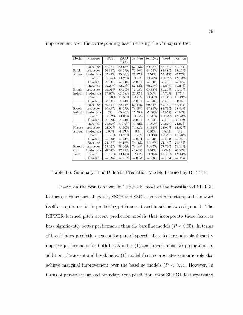
79
improvement over the corresponding baseline using the Chi-square test.
Model Measure POS SSCB SynFun SemRole Word PositionSSCL
Baseline 62.15% 62.15% 62.15% 62.15% 62.15% 62.15%Pitch Accuracy 76.31% 66.27% 72.36% 65.75% 82.58% 61.12%Accent Reduction 37.41% 10.88% 26.97% 9.51% 53.97% -2.75%
Conf. ±0.24% ±1.29% ±0.99% ±1.42% ±0.87% ±2.53%P-value < 0.01 = 0.04 < 0.01 = 0.08 < 0.01 = 0.64Baseline 62.23% 62.23% 62.23% 62.23% 62.23% 62.23%
Break Accuracy 69.01% 85.49% 70.13% 65.84% 80.26% 65.15%Index1 Reduction 17.95% 61.58% 20.92% 9.56% 47.74% 7.73%
Conf. ±1.96% ±0.51% ±0.78% ±1.67% ±1.30% ±1.13%P-value < 0.01 < 0.01 < 0.01 = 0.08 < 0.01 0.16Baseline 69.44% 69.44% 69.44% 69.44% 69.44% 69.44%
Break Accuracy 69.44% 88.07% 74.85% 67.81% 82.75% 68.84%Index2 Reduction 0% 60.96% 17.70% -5.30% 43.55% -1.96%
Conf. ±2.02% ±1.09% ±0.62% ±0.87% ±0.73% ±2.23%P-value < 0.96 < 0.01 < 0.01 < 0.43 < 0.01 < 0.79Baseline 71.82% 71.82% 71.82% 71.82% 71.82% 71.82%
Phrase Accuracy 72.05% 71.36% 71.82% 71.83% 72.05% 71.82%Accent Reduction 0.82% -1.63% 0% 0.04% 0.82% 0%
Conf. ±1.91% ±1.77% ±1.98% ±1.30% ±2.27% ±1.98%P-value = 0.99 = 0.94 = 0.94 = 0.94 = 0.99 = 0.94Baseline 74.16% 74.16% 74.16% 74.16% 74.16% 74.16%
Bound Accuracy 74.15% 78.66% 74.14% 74.42% 74.70% 74.14%ary Reduction -0.04% 17.41% -0.08% 1.01% 2.09% -0.08%Tone Conf. ±1.91% ±1.65% ±2.14% ±1.94% ±1.71% ±2.14%
P-value = 0.93 = 0.18 = 0.93 = 0.99 = 0.93 = 0.93
Table 4.6: Summary: The Different Prediction Models Learned by RIPPER
Based on the results shown in Table 4.6, most of the investigated SURGE
features, such as part-of-speech, SSCB and SSCL, syntactic function, and the word
itself are quite useful in predicting pitch accent and break index assignment. The
RIPPER learned pitch accent prediction models that incorporate these features
have significantly better performance than the baseline models (P < 0.05). In terms
of break index prediction, except for part-of-speech, these features also significantly
improve performance for both break index (1) and break index (2) prediction. In
addition, the accent and break index (1) model that incorporates semantic role also
achieve marginal improvement over the baseline models (P < 0.1). However, in
terms of phrase accent and boundary tone prediction, most SURGE features tested

80
do not show much predictive power. The only model which shows some promise is
the SSCB+SSCL boundary tone prediction model. It achieves 17.41% relative error
reduction, even though the improvement is not statistically significant (P = 0.18).
With a larger database (currently, there are only 356 intonational phrase boundaries
in the corpus), I expect that this performance may improve. In terms of error
reduction, the SSCB+SSCL break index (1) and (2) prediction models are the
best (61.58% and 60.96%). Other models which also achieved significant error
reduction include the word-accent model (53.97%), the word-break index (1) and
(2) model (47.74% and 43.55%), the POS-accent model (37.41%), and the syntactic
function-accent model (26.97%). From the data, I also found that the effectiveness
of these features in break index (1) prediction is consistently better than that in
break index (2) prediction. It may be due to the fact that detailed syntactic and
semantic information is more helpful in predicting fine-grained prosodic phrasing
(intermediate phrase v.s. intonational phrase). In the following, I inspect some of
the patterns learned by RIPPER.
4.2.3 Patterns learned by RIPPER
Most patterns learned in the POS-accent prediction model are consistent with pre-
vious findings. For example, the model accents content words like nouns, adjec-
tives, adverbs, cardinals while deaccenting function words like articles, conjunc-
tions, prepositions and pronouns. Thus, in general, it follows the content/function
word distinction. However, there is one exception to this. Verbs, which are content
words, are not accented, according to the POS pitch accent model.
In addition, the only meaningful rule (other than the default) learned by the

81
POS-break index (1) model predicts a significant prosodic phrase boundary after
a noun, which is an interesting finding. The POS-break index (2) model failed to
learn any useful rule. It is essentially the same as the baseline model.
In addition, the main rules learned by the SSCB+SSCL break index (1) pre-
diction model include “placing a significant prosodic phrase boundary at a sentence
boundary”, or “placing a significant boundary after a list item”. The rules also pre-
dict a significant boundary before or after a circumstantial, a predicate modifier,
a participant, a qualifier, a classifier, a describer and a possessor whose length is
greater than or equal to two. In terms of the rules learned for break index (2), the
rules place an intonational phrase boundary at the end of a sentence whose length
is greater than two words, or at the end of a list item whose length is equal to one,
or at the end of a qualifier whose length is greater than one, or at the end of a
circumstantial whose length is greater than one, or at the end of a list item whose
length is greater than two, or at the end of a participant whose length is greater
than three.
Syntactic function also proves to be a good predictor for both pitch accent
and break index prediction. In pitch accent prediction, the model deaccents words
whose syntactic function is neither the head nor the classifier of an object or subject.
It also deaccents words whose syntactic function is either a predicate or a clause-
conj. In break index prediction, the rules learned for break index (1) and (2) are
the same. The main rules assign a significant prosodic phrase boundary after both
an object head and subj-comp head. It is interesting to notice that both object and
subject-compliment usually are the second argument of a sentence; therefore, they
commonly occur later than subject in a sentence. Subject head does not have the

82
same property.
The word itself also proves to be a good predictor for both accent and break
index prediction. Typical words that are deaccented in the model include “the”,
“of”, “and”, “in” as well as “units”, “level”, “incision”, “savers”. Since the perfor-
mance of this model is the best among all the accent prediction models investigated,
it seems to suggest that for a CTS application like MAGIC, since it is only created
for a limited domain, specific features like word can be quite effective in prosody
prediction.
4.3 Summary
In this chapter, I primarily investigated the sentential semantic, syntactic and sur-
face features and their effects on prosody prediction. The modeling of semantic
and syntactic features are based on a general-purpose natural language generator
SURGE. I investigated how typical information represented in such a system helps
CTS prosody modeling.
Overall, based on the analysis results summarized in Table 4.5, most seman-
tic, syntactic and surface features tested show significant correlation with pitch
accent placement, break index, phrase accent and boundary tone assignment. More-
over, based on Table 4.6, by incorporating different semantic, syntactic and surface
futures, different prosody prediction models were able to improve the performance
of pitch accent and break index prediction significantly over the baseline models. On
the other hand, even some features show significant correlation with phrase accent
and boundary tone assignment, most of the prediction models were unable to learn
useful patterns. None, but one of the learned prediction models, the SSCB+SSCL

83
boundary tone prediction model, achieved some improvement over the majority-
based baseline (17.4%). This prediction model suggested placing a H% tone after a
single-word list item. Overall, it seems that more features are needed to account for
the variations in the phrase accent and boundary tone assignment. For example,
sentence type may be a good predictor of phrase accent and boundary tone. In
addition, in our corpus, some variations in phrase accent and boundary tone may
be due to intra speaker variation or factors that are not modeled.
Although the representation of these features may not be ideal for prosody
prediction because more fine-grained word class information may be more helpful
in prosody prediction, since SURGE is an independently motivated language gen-
eration system, it nonetheless provides valuable information on the typical features
a practical CTS system which employs general-purpose NL generators could expect
for its prosody modeling.

84
Chapter 5
Deep Semantic and Discourse
Features
In addition to the SURGE features, which are mostly at the sentence level, an
NLG system also produces deep semantic and discourse features. These features
are much harder to extract from a text, and therefore, primarily available to CTS
systems and not to TTS systems. In this section, I explore three such features:
semantic type, given/new, and semantic abnormality.
5.1 Feature Description
5.1.1 Semantic Type
One knowledge resource used by the MAGIC NL generator is its domain ontology.
This encodes the semantic types of different concepts in the domain. When a pa-
tient’s medical record is received, the system first instantiates the domain ontology

85
...
...
c-animatedc-status ...c-receive
c-humanc-med-status
c-patientc-postcabg-status ...
...
c-has-attribute c-human-activity ... c-abstract c-physical
c-thing
c-state c-event c-entity
...
...
...
Figure 5.1: A Segment of the MAGIC Ontology
with a patient’s data. As a result, the instantiated ontology contains not only the
data in the medical record but also their associated semantic types as well as their
relations with the other concepts in the domain. Figure 5.1 shows a segment of the
MAGIC domain ontology.
To explore the usefulness of semantic types in prosody modeling, a script
was designed to automatically extract the most specific semantic type of a concept
from a MAGIC output FD. For example, in the following sentence “John Herman
is a fifty one year old male patient of Dr. Smith undergoing CABG”, “John Her-
man” has a semantic type of “c-name”1 The semantic type of “is” is “c-is-a”. In
addition, “c-age”, “c-gender”, “c-patient”, “c-name” and “c-operation” are the se-
mantic types for “fifty one year old”, “male”, “patient”, “Dr. Smith”, and “CABG”
respectively. In general, all the words realizing an input entity have the semantic
type of that entity. If a word does not belong to any of the input data, it is assigned
a special semantic type.
Since the same semantic type may be shared by different surface words (for
1The prefix c- is used to distinguish the concept “name” with the word “name”.

86
example, the semantic type for both male and female is c-gender), the semantic
type provides a level of generalization over surface realization and it may be useful
for prosody modeling. Intuitively, we may expect that words sharing the same
semantic type may also share similar prosodic properties. For example, “male”
and “female” are more likely to have similar accentual patterns as “male” and
“hypertensive”, which do not share the same semantic type.
5.1.2 Given/New
The second feature I explored is a word’s given/new status. As [Prince, 1981; 1992;
Brown, 1983] have pointed out, there are various methods of ascertaining what
should be regarded as given or new. Based on Prince, an entity can be discourse-
old (new) if it has (not) been activated in the prior discourse stretch; or it can
be hearer-old (new) if a speaker presumes that a hearer knows (does not know)
the information; or inferable, if it is recoverable from a hearer’s background or
conversational environment. Because the current MAGIC NL generator does not
model hearer old/new, or inferable status, in the following analysis, I focus on the
discourse given/new distinction. Since discourse given/new is not easy to parse from
a text, only a few TTS systems to date incorporate such a feature [Hirschberg, 1993].
Moreover, TTS given/new status is mostly inferred based on lexical repetition while
in MAGIC, since each concept has an unique concept id, its given/new status is
automatically produced based on concept repetition.
Since the given/new distinction primarily involves content words, in the
given/new analysis, only the content words were examined. For example, if a con-
cept is given, then all the content words realizing that concept are given. Similarly,

87
all the content words realizing a new concept are new.
5.1.3 Semantic Abnormality
Another type of deep semantic information is semantic abnormality. In MAGIC,
semantic abnormality was defined as the unexpectedness of medical events or condi-
tions. Compared with other features investigated in this study, semantic abnormal-
ity defined in this way is clearly domain-dependent. For example, for the general
population, blood pressure of 170/100 is considered high and therefore, abnormal.
However, patients who need cardiac surgery usually have severe heart problems,
so for them such a value may be considered relatively normal. Furthermore, if a
patient’s condition is unexpectedly good or bad, both are categorized as abnormal.
Identifying abnormality in general is non-trivial. In MAGIC, this task is performed
by domain experts.
5.2 Analysis
In this section, I investigate the usefulness of semantic type, given/new, and se-
mantic abnormality in prosody prediction. Similar to the previous chapter, I use
both statististical correlation tests as well as RIPPER to analyze the relationship
between prosody and these deep semantic and discourse features. Since the anal-
ysis of semantic abnormality in prosody modeling is quite new and, thus far, this
feature is not modeled in the MAGIC NL generator, only manually annotated ab-
normality information is used for the current study. Since the investigation led us
to study a new set of prosodic features, I will discuss the prosodic correlates of

88
Variables Chi-squared df p-value
Given/New and Pitch Accent 54.32 1 p < 0.01Given/New and Break Index(1) 41.20 1 p < 0.01Given/New and Break Index(2) 33.66 1 p < 0.01Given/New and Phrase Accent 1.12 1 p < 0.30Given/New and Boundary Tone 1.96 1 p < 0.17
Table 5.1: The Correlations between Given/new and Prosody
semantic abnormality separately from semantic type and given/new. Also, when
exploring semantic type, since there are a total of 62 different semantic types in the
read speech corpus, the contingency tables for semantic type and different prosodic
features are too sparse to apply the Chi-square test properly. Thus, only RIPPER
is used for this analysis. Both the correlation test and RIPPER are used for the
given/new analysis.
5.2.1 Correlation Analysis for Given/new
To test the correlation between discourse given/new and pitch accent, I used the
Chi-square test. Table 5.1 shows that discourse given/new is significantly correlate
with pitch accent and break index with p < 0.01. However, since given/new does
not significantly correlated with phrase accent and boundary tone prediction, in
the following analyses, I will only focus on pitch accent and break index prediction.
5.2.2 RIPPER Analysis for Semantic Type and Given/New
The machine learning experiments whose results are shown in Table 5.2 indicate
that semantic type is a useful predictor for pitch accent and break index predic-
tion. Models with semantic type information achieved significant improvement over

89
the baseline models in accent and break index prediction. However, even though
the correlation results seem to suggest that discourse given/new is significantly as-
sociated with pitch accent and break index prediction, the RIPPER experiments
did not confirm this. It may be that the current data set is too small to draw a
conclusion.
Model Measures Semantic Type Given/New
Baseline 62.15% 79.03%Pitch Accuracy 70.21% 79.03%Accent Err. Reduction 21.29% 0%
Conf. Int. ±1.46% ±0.66%P-value P < 0.01 P = 0.95Baseline 62.23% 53.20%
Break Accuracy 70.99% 56.62%Index(1) Err. Reduction 23.19% 7.1%
Conf. Int. ±1.86% ±0.69%P-value P < 0.01 P = 0.19Baseline 69.44% 59.08%
Break Accuracy 75.28% 59.08%Index(2) Err. Reduction 19.11% 0%
Conf. Int. ±0.72% ±2.10%P-value P < 0.01 P = 0.96
Table 5.2: Summary: The Different Prediction Models Learned by RIPPER
5.2.3 Semantic Abnormality and Prosody
To empirically investigate how semantic abnormality is related to prosody, a por-
tion of the spontaneous speech corpus was used. Based on ToBI break indices,
utterances in the corpus were first separated into intermediate (minor) phrases.
As a result, the basic units in this study are intermediate phrases. Then a doc-
tor was asked to categorize whether the information conveyed in each intermediate
phrase was abnormal (1) or not (0). Sometimes, the doctor assigned a single tag to
several adjacent intermediate phrases because each phrase by itself did not contain
enough information to make a judgment. The final corpus includes 784 intermediate

90
phrases, 114 of which are categorized as abnormal, and all of which are annotated
with both semantic abnormality and ToBI prosodic features.
5.2.3.1 Prosodic Features
Based on informal observations, semantic abnormality may be associated with a
combination of prosodic features that appear to be intended to draw the listener’s
attention to the information being conveyed. For example, in addition to ToBI
features, speaking rate, pitch range, and F0 changes can all be used to highlight
unusual information in speech. A speaker may increase or decrease her speaking
rate. In addition, expanded pitch range, increase in loudness, and increase in the
number of accented items, and more frequent pauses often appeared to be associated
with information the speaker wished to make more prominent. So, these features
were the candidates for our investigation.
Of all the features I investigated, some of them, such as HiF0, the break
index before, the break index after, and accent probability, are derived from ToBI
annotations. The HiF0 of an intermediate phrase is defined as the maximum F0
within the most prominent pitch accent in an intermediate phrase which contains
a high (H) tone. It is a more robust measure of a speaker’s pitch range than
the highest F0 value of an intermediate phrase. The next two features, the break
index before and after an intermediate phrase, measure the strength of the prosodic
phrase boundary preceding or ending an intermediate phrase. By definition, their
values can only be 3 or 4. The next feature, the accent probability, is defined as
the percentage of words that are accented in an intermediate phrase. In addition
to these ToBI-based features, 3 additional acoustic features, average speaking rate,

91
Prosodic Features ρ P-value
Speaking Rate 0.02 0.60HiF0 0.13 < 0.01
RMS total 0.0022 0.96F0 total 0.12 < 0.01
Break Index Before -0.08 0.05Break Index After 0.086 0.04Accent Probability -0.04 0.32
Table 5.3: Abnormality and Prosodic Features.
RMS total, and F0 total, were also investigated. The average speaking rate is
measured as the number of syllables per second of an intermediate phrase. Both
the RMS total and F0 total are automatically computed from wave files for each
intermediate phrase. Intuitively, we may expect that low speaking rate, high HiF0,
high RMS and F0 total, larger break index before and after a phrase, and high
accent probability may signal abnormality. Finally, to reduce the influence of inter-
speaker variations, I normalized those speaker-dependent features such as speaking
rate, HiF0, RMS total and F0 total, before conducting the empirical analysis. I use
a quite crude method for normalization. First, I compute the average value for each
feature in each speech file. For example, in terms of pitch range, I compute the
average HiF0 as the speaker-specific reference value. Then, the normalized value is
the ratio between the real value and the average value.
To understand how prosodic features are associated with abnormality, I per-
formed a set of correlation analyses based on Spearman’s rank-based correlation
test. The test results shown in Table 5.3 present the correlation coefficient ρ and
its associated statistical significance p-value for each feature.
The test results demonstrate that HiF0, F0 total, Break Index Before, and
Break Index After are significantly correlated with abnormality with p− value <=

92
0.05. Since their correlation coefficients are positive, higher HiF0, higher F0 total
and more significant break index afterwards are more likely to co-occur with ab-
normal information (ρ > 0). However, for break index before, although it shows a
certain degree of correlation, the association is negative (ρ < 0), which means the
break index is less significant before phrases containing abnormal information. This
result is not what I expected because intuitively we might think that significant
prosodic phrase boundaries should be associated with important information.
To explain the negative correlation between break index before and abnor-
mality, I re-examine the data. After analyzing the corpus, it seems that the negative
correlation is a result of using break index in simultaneously conveying several kinds
of information, such as information structure, semantic/syntactic structure, as well
as information importance. In the corpus, many sentences follow the following pat-
tern: theme + rheme. Theme is the current topic as well as the connector to the
context. In contrast, rheme communicates new information about a theme. Thus,
based on the definition of abnormality, rhemes should be considered more impor-
tant. Here is an utterance from our corpus: “(He is uh) (a heavy alcohol drinker)”.
“He is uh” is the theme, and “a heavy alcohol drinker” is the rheme. Prosodically,
the utterance consists of two intermediate phrases: “He is uh” and “a heavy al-
cohol drinker”. Since the boundary before “He is uh” is a sentence boundary, its
break index is almost always “4”. While the break index before “a heavy alcohol
drinker” usually is less significant (can be either “3” or “4”). In term of semantic
abnormality, however, the first phrase was labeled as normal and the second one
was abnormal. Thus, there exists a mild negative correlation between abnormality
and the break index.

93
Moreover, the strength of a break index is also affected in part by an ut-
terance’s semantic and syntactic structure. Based on our corpus, a significant
prosodic phrase boundary is often associated with a significant syntactic and se-
mantic constituent boundary. For example, a sentence boundary is often signaled
by a significant prosodic phrase boundary (100% in the break index1 model). Cir-
cumstantial boundaries are also frequently communicated by a significant prosodic
phrase boundary (100% in the break index1 model). In contrast, the prosodic
phrase boundary associated with a word boundary usually is insignificant (only has
6.43% chance to be significant in the break index1 model). After analyzing the
corpus, it seems that significant prosodic phrase boundaries that are not licensed
by the utterance’s syntactic/semantic structure may signal abnormality.
To verify that not only the absolute break index but also the break index
difference are important in conveying abnormality, I conducted a set of experi-
ments. Before proceeding with the statistical analysis, I manually cleaned all the
utterances in the corpus. All the disfluencies and repairs were removed and the
clean corpus contained only grammatical sentences or sentence segments. Then
I assigned a semantic/syntactic constituent boundary (SSCB) to all locations be-
tween two adjacent words. The index of SSCB was decided based on the rank of
each SSCB. Finally the difference between the break index used by the speaker and
its semantic/syntactic boundary index was computed. Based on this information, I
tested two new variables: the boundary difference before and after an intermediate
phrase. Table 5.2.3.1 shows the results of the correlation tests.
Based on the results, the boundary difference before a phrase is significantly
associated with abnormality. The larger the difference is, the more likely it will be

94
Prosodic Features ρ P-value
Boundary Difference Before 0.125 P < 0.01Boundary Difference After -0.04 P = 0.29
Table 5.4: Abnormality and Index Difference.
followed by a piece of abnormal information. The other new feature, the boundary
difference after a phrase, however, does not seem to signal abnormality. I speculate
that the above association patterns may be due to the nature of the speech corpus.
Usually, the doctors do not intentionally draw attention before abnormal informa-
tion. However, the doctors may unintentionally pause before abnormal information
to think about the content, even though it may occur at an “inappropriate” place
for a pause, such as after an article. This may explain why significant break index
difference before is a good predictor of abnormality.
5.3 Summary
In this chapter, I investigated three additional features: semantic type, discourse
given/new and semantic abnormality. Even with only limited data, the results
suggest that semantic types are useful for both pitch accent and break index pre-
diction. In addition, semantic abnormality is also significantly associated with a
set of prosodic features, such as break index difference, HiF0 and total F0. Finally,
the results did not confirm the usefulness of discourse given/new. This may also
be due to the sparse data problem.

95
Chapter 6
Modeling Features Statistically
for Prosody Prediction
In the previous chapters, I described empirical results on the effects of features
from a natural language generator on prosody prediction. In this section, I expand
the discussion to cover a few new features. As I stated before, the main reason for
modeling features not covered by existing NLG systems is to improve a language
generator’s capability in producing spoken language. Since many existing language
generation tools are designed for text generation, they do not specifically model
features that affect mainly speech features, such as pronunciation and prosody.
In this chapter, I focus on two such features which have the potential to
affect prosody prediction: the semantic informativeness and the predictability of
a word. Since the usefulness of these features in prosody modeling, pitch accent
in particular, has been previously suggested [Bolinger, 1958; 1972b; 1972a; Ladd,
1996], in this chapter, I focus on empirically investigating the usefulness of these
features in pitch accent prediction.

96
The procedure used to define or compute these features is quite different
from what I used in the previous chapters. Otherwise, I adopted a similar routine
to examine their usefulness in pitch accent prediction. I use both statistical tests as
well as RIPPER to analyze the influence of these features in pitch accent prediction.
Overall, three corpora are used in the study: the text corpus, which is used to
statistically define, or compute the new features; the read and spontaneous corpora,
which are used to empirically verify their usefulness in pitch accent prediction.
Again, the focus of this investigation is on pitch accent placement.
6.1 Word Informativeness
Linguists have speculated that relative informativeness, or semantic weight of a
word can influence accent placement. Ladd [1996] claims that “the speakers as-
sess the relative semantic weight or informativeness of potentially accentable words
and put the accent on the most informative point or points” (ibid, pg. 175).
He also claims that “if we understand relative semantic weight, we will auto-
matically understand accent placement” (ibid, pg. 186). Bolinger [1958; 1972b;
1972a] also stated “My position was–and is– that the location of sentence accents
is not explainable by syntax or morphology .... I have held, with Hultzen 1956,
that what item has relatively stronger accent in the larger intonational pattern is
a matter of information, not of structure....” He also uses the following examples
to illustrate the phenomenon:
1. He was arrested because he KILLED a man.
2. He was arrested because he killed a POLICEMAN.

97
The capitalized words in the examples are accented. In the first example, man is
semantically empty relative to kill; therefore, the verb kill gets accented. However,
in the second example, policeman is semantically rich and is accented instead.
However, different theories, not based on informativeness, were proposed to
explain the above phenomenon. For example, Bresnan’s [1971] explanation is based
on syntactic function. She suggests that man in the above sentence does not get
accented because man and other words like guy or person or thing form a category
of “semi-pronouns”. Similarly, in [Monaghan, 1994], a special class was created for
semantically empty content words for pitch accent prediction.
While researchers have discussed the possible influence of semantic informa-
tiveness, there has been no known empirical study of the claim nor has this type of
information been incorporated into computational models of prosody. In this work,
I employ two measurements of informativeness. First, I adopt an information-based
framework [Shannon, 1948], quantifying the “Information Content (IC)” of a word
as the negative log likelihood of a word in a corpus. The second measurement
is TF*IDF (Term Frequency times Inverse Document Frequency) [Salton, 1989;
1991], which has been widely used to quantify word importance in information
retrieval tasks. Both IC and TF*IDF are well established measurements of infor-
mativeness and therefore, good candidates to investigate. The results of this study
show that word informativeness not only is closely related to word accentuation,
but also provides new power in pitch accent prediction. The experimental results
suggest that information content is a valuable feature to be incorporated in speech
synthesis systems.

98
In the following sections, I first define IC and TF*IDF. I then describe a set
of experiments conducted to study the relation between informativeness and pitch
accent. I explain how machine learning techniques are used in the pitch accent
modeling process. The results show that:
• Both IC and TF*IDF scores are strongly correlated with pitch accent assign-
ment.
• IC is a more powerful predictor than TF*IDF.
• IC provides better prediction power in pitch accent prediction than previous
techniques.
The investigated pitch accent models can be easily adopted by both CTS and TTS
systems.
6.1.1 Definitions of IC and TF*IDF
Following the standard definition in information theory [Shannon, 1948; Fano, 1961;
Cover and Thomas, 1991] the IC of a word is
IC(w) = −log(P (w))
where P (w) is the probability of the word w appearing in a domain and P (w) is
estimated as: F (w)N
where F (w) is the frequency of w in the corpus and N is the
accumulative occurrence of all the words in the corpus. Intuitively, if the probability
of a word increases, its informativeness decreases and therefore it is less likely to be
an information focus. Similarly, it is therefore less likely to be communicated with
pitch prominence.

99
TF*IDF is defined by two components multiplied together. TF (Term Fre-
quency) is the word frequency within a document; IDF (Inverse Document Fre-
quency) is the logarithm of the ratio of the total number of documents to the
number of documents containing the word. The product of TF*IDF is higher if a
word has a high frequency within the document, which signifies high importance
for the current document, and low dispersion in the corpus, which signifies high
specificity. In this research, I employed a variant of TF*IDF score used in SMART
[Buckley, 1985], a popular information retrieval package:
(TF*IDF)wi,dj=
(1.0 + log Fwi,dj) log
N
Nwi√√√√ M∑k=1
((1.0 + log Fwk,dj) log
N
Nwk
)2
where Fwi,djis the the frequency of word wi in document dj, N is the total number
of documents, Nwiis the number of documents containing word wi and M is the
number of distinct stemmed words in document dj.
IC and TF*IDF capture different kinds of informativeness. IC is a metric
global in the domain of a corpus and each word in a corpus has a unique IC score.
TF*IDF captures the balance of a metric local to a given document (TF) and a
metric global in a corpus (IDF). Therefore, the TF*IDF score of a word changes
from one document to another (different TF). However, some global features are
also captured by TF*IDF. For example, a common word in the domain tends to
get a low TF*IDF score in all the documents in the corpus.
In order to empirically study the relations between word informativeness
and pitch accent, both the read and spontaneous speech corpora as well as the

100
text corpus are used1. The orthographic transcripts of the speech corpora as well
as the text corpus are used to calculate the IC and TF*IDF scores. First, all
the words in the text corpus as well as the speech transcripts are processed by a
stemming model so that words like receive and receives are treated as one word.
I employ a revised version of Lovins’ stemming algorithm [Lovins, 1968] which
is implemented in SMART. Although the usefulness of stemming is arguable, I
choose to use stemming because I think, for example, receive and receives may be
equally likely to be accented. Then, IC and TF*IDF are calculated. After this,
the effectiveness of informativeness in accent placement is verified using the speech
corpora. Each word in the speech corpora has an IC score, a TF*IDF score, a part-
of-speech (POS) tag and a pitch accent label. Both IC and TF*IDF are used to test
the correlation between informativeness and accentuation. POS is also investigated
by RIPPER in automatic pitch accent modeling.
6.1.2 Experiments
I conducted a series of experiments to determine whether there is a correlation
between informativeness and pitch accent and whether informativeness provides an
improvement over other known indicators on pitch accent, such as part-of-speech.
6.1.2.1 Ranking Word Informativeness in the Corpus
Table 6.1 and 6.2 show the most and least informative words in the corpus. The
IC order indicates the rank among all the words in the corpus, while TF*IDF
order in the table indicates the rank among the words within a document. The
1In this study, only a subset of the spontaneous speech corpus as well as a subset of the textcorpus were used due to the availability of the data at the time the experiments were conducted

101
Rank IC Most Informative IC Least Informative
1 zophrin with2 name1 on3 xyphoid patient4 wytensin in5 pyonephritis she6 orobuccal he7 tzanck for8 synthetic no9 Rx day10 quote had
Table 6.1: IC Most and Least Informative Words
Rank TF*IDF Most Informative TF*IDF Least Informative
1 your and2 vol a3 tank the4 sonometer to5 papillary was6 pancuronium of7 name2 with8 name3 in9 incomplete old10 yes year
Table 6.2: TF*IDF Most and Least Informative Words
document was picked randomly from the corpus. In general, most of the least
informative words are function words, such as with or and. However, some content
words are selected, such as patient, year, old. These content words are very common
in this domain and are mentioned in almost all the documents in the corpus. In
contrast, the majority of the most informative words are content words. Some of
the selections are less expected. For example your ranks as the most informative
word in a document using TF*IDF. This indicates that listeners or readers are
rarely addressed in the corpus. This word appears only once in the entire corpus.

102
6.1.2.2 Testing the Correlation of Informativeness and Accent Predic-
tion
Feature Correlation Coefficient Significance Level
TF*IDF ρ = 0.29 p < 0.01IC ρ = 0.34 p < 0.01
Table 6.3: The Correlation of Informativeness and Accentuation
In order to verify whether word informativeness is correlated with pitch
accent, I employ Spearman’s rank correlation coefficient ρ and associated test
[Conover, 1999] to estimate the correlations between IC and pitch prominence as
well as TF*IDF and pitch prominence. As shown in Table 6.3, both IC and TF*IDF
are closely correlated to pitch accent with a significance level p < 0.01. Because
the correlation coefficient ρ is positive, this indicates that the higher the IC and
TF*IDF are, the more likely a word is to be accented.
6.1.2.3 Learning IC and TF*IDF Accent Models
The correlation test suggests that there is a statistically significant correlation be-
tween informativeness and pitch accent. In addition, I also want to show how
much performance gain can be achieved by adding this information to pitch accent
models. To study the effect of TF*IDF and IC on pitch accent, I use RIPPER
to learn models that predict the effect of these indicators on pitch accent. The
results were reported based on cross-validation. In this experiment, the predictors
are IC or TF*IDF, and the response variable is the pitch accent assignment. Once
a set of RIPPER rules are acquired, it can be used to predict which word should
be accented in a new corpus.

103
Models RIPPER Performance
Baseline 52.02%TF*IDF Model 65.66%
IC Model 70.06%function/content model 69.42
Table 6.4: Comparison of the IC, TF*IDF Models with the Baseline Model
I also use a majority-based baseline model where all words are assigned a
default accent status (accented). 52% of the words in the corpus are actually
accented and thus, the baseline has a performance of 52%. The results in Table 6.4
show that when TF*IDF is used to predict pitch accent, performance is increased
over the baseline of 52% to 65.66 % . In the IC model, the performance is further
increased to 70.06%. Two conclusions can be drawn from the results. First, both
IC and TF*IDF are effective in pitch accent prediction. All the improvements over
the baseline model are statistically significant with p < 0.01. Second, the IC model
is more powerful than the TF*IDF model. It out performs the TF*IDF model
with p < 0.01 for the RIPPER model. The low p-values show the improvements
achieved by the IC models are significant. Since IC performs better than TF*IDF in
pitch accent prediction, I choose IC to measure informativeness in all the following
experiments.
I also compared the IC and TF*IDF model with the Function/Content
model. In the Function/Content model, all the content words are accented while
function words are not. The Function/Content model is a simple yet effective model
and has been employed in speech synthesis systems before. The comparison shows
that the performance of the IC model is better than that of the Function/Content
models. However the significance of the difference needs to be tested in a larger

104
corpus. The performance of the TF*IDF model is significantly lower than that of
the Function/Content models with P¡0.01. I can conclude from this comparison
that the IC model is as effective as the function/content model in pitch accent pre-
diction. However, the TF*IDF model is slightly worse than the Function/Content
model.
6.1.2.4 Incorporating IC in Reference Accent Models
In order to show that IC provides additional power in predicting pitch accent than
current models, I directly compare the influence of IC with that of other reference
models. In this section, I describe experiments that compare IC alone against a
part-of-speech (POS) model for pitch accent prediction and then compare a model
that integrates IC with POS against the POS model. Finally, anticipating the pos-
sibility that other features within a traditional TTS in combination with POS may
provide equal or better performance than the addition of IC, I carried out experi-
ments that directly compare the performance of Text-to-Speech (TTS) synthesizer
alone with a model that integrates TTS with IC.
In most speech synthesis systems, part-of-speech (POS) is the most effective
feature in pitch accent prediction. Therefore, showing that IC provides additional
power over POS is important. In addition to the importance of POS within TTS
for predicting pitch accent, there is a clear overlap between POS and IC. I have
shown that the words with highest IC usually are content words and the words with
lowest IC are frequently function words. This is an added incentive for comparing
IC with POS models. Thus, I want to explore whether the new information added
by IC can provide any improvement when both of them are used to predict accent

105
assignment.
Models RIPPER Performance
IC Model 70.06%POS Model 70.52%
POS+IC Model 73.71%
Table 6.5: Comparison of the POS+IC Model with the POS Model
Models RIPPER Performance
TTS Model 71.75%TTS+IC Model 72.75%POS+IC Model 73.71%
Table 6.6: Comparison of the TTS+IC Model with the TTS Model
As shown in table 6.5, the performance of the POS model is 70.52% , which is
comparable with that of the IC model. This comparison further shows the strength
of IC because it has similar power to POS in pitch accent prediction and it is easy
to compute. When the POS models are augmented with IC, the POS+IC model
performance is increased to 73.71%. The improvement is statistically significant
with p = 0.01 which means the new information captured by IC provides additional
predicting power for the POS+IC models. These experiments produce new evidence
confirming that IC is a valuable feature in pitch accent modeling.
I also tried another reference model, Text-to-Speech (TTS) synthesizer out-
put, to evaluate the results. The TTS pitch accent model is more comprehensive
than the POS model. It has taken many features into consideration, such as dis-
course and semantic information. It is well established and has been evaluated
in various situations. In this research, I adopted Bell Laboratories’ TTS system
[Sproat, 1997; Olive and Liberman, 1985; Hirschberg, 1990b]. I ran it on the speech

106
transcript to get the TTS pitch accent assignments. Comparing the TTS accent as-
signment with the expert accent assignment, the TTS performance is 71.75% which
is lower than the POS+IC model. I also tried to incorporate IC in the TTS model.
A simple way of doing this is to use the TTS output and IC as predictors and train
them with the data. The obtained TTS+IC model achieves marginal improvement.
The performance of TTS+IC model increases to 72.75%, which is lower than that
of the POS+IC models. I speculate that this may be due to the corpus I used. The
Bell Laboratories’ TTS pitch accent model is trained in a totally different domain,
and the medical corpus seems to negatively affect the TTS performance (71.75%
compared to 80% to 85%, its normal performance [Hirschberg, 1993]). Since the
TTS+IC models involve two totally different domains, the effectiveness of IC may
be compromised. If this assumption holds, I think that the TTS+IC model will
perform better when IC is trained together with the TTS internal features on the
corpus directly. But since this requires retraining a TTS system for a new domain
and it is hard to conduct such an experiment, no further comparison was conducted
to verify this assumption.
Although TF*IDF is less powerful than IC in pitch accent prediction, since
they measure two different kinds of informativeness, it is possible that a TF*IDF+IC
model can perform better than the IC model. Similarly, if TF*IDF is incorporated
in the POS+IC model, the overall performance may increase for the combined
POS+IC+TF*IDF model.
The performance of TF*IDF+IC and POS+IC+TF*IDF model is 70.42%
and 74.20% respectively, which are not almost the same as the original models.
This result seems to suggest that IC is the dominant predictor when both IC and

107
TF*IDF are presented. It is further confirmed when the RIPPER learned rules were
inspected. For the TF*IDF+IC model, of all the 76 rules produced by RIPPER
during cross-validation, only 3.9% rules use TF*IDF and only 1.8% of the conditions
include TF*IDF score. However 100% rules use IC and 98.2% conditions include
IC. Similarly for the POS+IC+TF*IDF model, of all the 72 rules learned during
cross-validation, TF*IDF is only used in one rule in one condition, IC is used in
86.1% of the rules and 67.9% of the conditions and POS is used in 72.2% of the
rules and 31.3% of the conditions. This result shows that TF*IDF is not very useful
when IC is presented in pitch accent prediction.
6.1.3 Summary and Discussion
In this section, I have provided empirical evidence for the usefulness of informative-
ness for accent assignment. Overall, there is a positive correlation between indica-
tors of informativeness, such as IC and TF*IDF, and pitch accent. The more infor-
mative a word is, the more likely that a pitch accent is assigned to the word. Both
of the two measurements of informativeness improve over the baseline performance
significantly. I also show that IC is a more powerful measure of informativeness
than TF*IDF for pitch accent prediction. Later, when comparing IC-empowered
POS models with POS models, I found that IC enables additional, statistically
significant improvements for pitch accent assignment. This performance also out-
performs the TTS pitch accent model. Overall, IC is not only effective, as shown
in the results, but also relatively inexpensive to compute for a new domain.
IC does not directly measure the informativeness of a word. It measures
the rarity of a word in a corpus. That a word is rare doesn’t necessarily mean

108
that it is informative. Semantically empty words can be ranked high using IC as
well. For example, CABG is a common operation in this domain. CABG is almost
always used whenever the operation is mentioned. However, in a few instances,
it is referred to as a CABG operation. As a result, the semantically empty word
(in this context) operation gets a high IC score and it is very hard to distinguish
high IC scores resulting from this situation from those that accurately measure
informativeness and this causes problems in precisely measuring the IC of a word.
Similarly, misspelled words also can have high IC score due to their rarity.
A second issue concerns the use of the TF*IDF score for this application.
TF*IDF should rank topic related words higher. Topic words identified in this
way have a high frequency in the current document (high TF) and low occurrence
in other documents (high IDF score). However, topic words are not necessarily
communicated by pitch prominence. On the contrary, each time a word is repeated
in a document (increased TF), the information gain becomes less and less. As a
result, it is less likely associated with pitch accent. If this assumption is true, I
speculate that IDF alone can be used instead and it might out-perform TF*IDF in
predicting accent.
Another issue concerns the reduction of noise in calculating IC or TF*IDF.
For example, if took and take are treated as two different words, the IC score will be
over-stated and TF*IDF score can be either over-stated or under-stated. Therefore,
a better morphology module can help reduce this type of noise.
IC may not be perfect for quantifying word informativeness. However, even
with a perfect measurement of informativeness, there are still many cases where
this information by itself would not be enough. For example, each word only
109
gets a unique IC score regardless of its context; yet it is well known that context
information plays a role in accentuation. As a result, it is also interesting to find
out how IC interacts with other features in accent prediction.
6.2 Word Predictability
In this section, I investigate how another feature, word predictability, influences
whether it should be accented or not. Modeling word predictability can be very
complicated. For example, discourse context, conversation environment, sentence
structure, as well as the background shared between a speaker and listener may all
affect the predictability of a word. In this study, I focus on the influence of a word’s
local context on accent prediction. More specifically, I focus on the influence of the
neighboring words. Results of experiments on two transcribed speech corpora in a
medical domain show that such predictability information is a useful predictor of
pitch accent placement.
6.2.1 Motivation
Previous researchers have speculated that word predictability affects accent assign-
ment. For example, Bolinger argued that the relatively more unpredictable items
in an utterance are more likely to be accented [Bolinger, 1972b; 1972a]. Some
examples which can support this claim are listed in the following:
1. a POINT to make
2. a point to ELUCIDATE

110
In the first example, the verb make is relatively predictable from POINT; therefore,
POINT receives the primary accent. In contrast, the verb ELUCIDATE is relatively
hard to predict from point, it receives the primary stress instead.
James Marchand [Marchand, 1993] also notes how word predictability, mea-
sured by word collocations, affect accent placement. He states familiar collocations
change their stress, witness the American pronunciation of ‘Little House’ [in the
television series Little House on the Prairie], where stress used to be on HOUSE,
but now, since the series is so familiar, is placed on the LITTLE. That is, for col-
located words, stress shifts to the left element of the compound. In other words,
since “LITTLE” and “house” have co-occurred many times, house becomes rela-
tively predictable, therefore does not receive primary accent any more. However,
there are numerous counter-examples: consider apple PIE, which retains a right
stress pattern, despite the collocation. Similarly in the following examples:
1. FIFTH street
2. fifth AVENUE
both Fifth Street and Fifth Avenue are two roads in New York City. Fifth Avenue
is more famous and thus frequently mentioned. In these two examples, the more
predictable word, such as AVENUE retain the primary accent while the less pre-
dictable word street does not receive a primary accent. So, the extent to which
word predictability affects accent patterns is still unclear.
Despite some preliminary investigation [Liberman and Sproat, 1992], word
predictability, or word collocation information has not, to my knowledge, been suc-
cessfully used to model pitch accent assignment; nor has it been incorporated into

111
any existing speech synthesis systems for accent prediction. In this paper, I empir-
ically verify the usefulness of word predictability for accent prediction. In Section
6.2.2, I present a short description of the predictability measures investigated. Sec-
tion 6.2.3 to 6.2.6 describe the analyses and machine learning experiments in which
I attempt to predict pitch accent placement. In Section 6.2.7 I sum up the results.
In the following, I focus on empirically investigating whether word pre-
dictability, based on a word’s local context, affects its accent patterns. More specif-
ically, in the following, I focus on how word predictability influences whether nouns
are accented or not.
Determining which nouns are accented and which are not is challenging,
since part-of-speech information cannot help here. So, other accent predictors must
be found. There are some advantages in looking only at one word class. The
interaction between part-of-speech and word predictability is eliminated, so that
the influence of word predictability is easier to identify. It also seems likely that
word predictability may have a greater impact on content words, like nouns, than
on function words, like prepositions. Thus, focusing on nouns seems a reasonable
starting point. Again, in this study, I used only binary accent/deaccent decisions.
6.2.2 Word predictability Measures
I used three measures of word predictability to examine the relationship between
word predictability and accent placement: word N-gram predictability, mutual in-
formation, and the Dice coefficient. Both mutual information [Fano, 1961] and the
Dice coefficient [Dice, 1945] are two standard measures of collocation. In general,
mutual information measures uncertainty reduction or departure from indepen-

112
dence. The Dice coefficient is a collocation measure widely used in information
retrieval [Salton and McGill, 1983]. In general there is some correlation between
word collocation and word predictability. For example, if two words are collocated,
then it will be easy to predict the second word from the first. Similarly, if one word
is highly predictable given another word, then there is a higher possibility that
these two words are collocated. Therefore, collocation measures, such as mutual
information and Dice coefficient, can be used as measures of word predictability.
N-gram word predictability has been widely used in language modeling for speech
recognition. In the following, I will give detailed definitions of each.
6.2.2.1 N-gram Predictability
Statistically, Ngram word predictability is defined as the log conditional probability
of word wi, given the previous words wi−1, wi−2...:
Pred(wi) = log(Prob(wi|wi−1wi−2...wi−n)
Depending on the number of context words involved, N-gram predictability be-
comes unigram predictability if n=0, or bigram predictability if n=1 or trigram
predictability if n=2. N-gram predictability directly measures the likelihood of
seeing one word, given the occurrence of zero or several previous words. N-gram
predictability has two forms: absolute and relative. Absolute predictability is the
value directly computed from the formula. For example, given four adjacent words
wi−1, wi, wi+1 and wi+2, if I assume bigram predictability Prob(wi|wi−1) = 0.0001,
Prob(wi+1|wi) = 0.001, and Prob(wi+2|wi+1) = 0.01, the absolute bigram pre-
dictability will be -4, -3 and -2 for wi, wi+1 and wi+2. The relative predictability
is defined as the rank of absolute predictability among words in a constituent. In

113
the same example, the relative bigram predictability will be 1, 2 and 3 for wi, wi+1
and wi+2, where 1 is associated with the word with the lowest absolute predictabil-
ity. In general, the higher the rank, the higher the absolute predictability. Except
in Section 6.2.6, all the predictability measures mentioned in this paper use the
absolute form.
I used the text corpus to compute N-gram word predictability for our med-
ical domain. Three N-gram predictability measures were computed: unigram pre-
dictability, bigram predictability, and trigram predictability. In the following anal-
ysis, I focus on bigram predictability because both mutual information and Dice
coefficient only use one context word. When calculating the word bigram pre-
dictability, I first filtered uncommon words (words occurring 5 times or fewer in
the corpus) then used the Good-Turing discount strategy to smooth the bigram.
Finally I calculated the log conditional probability of each word as the measure of
its bigram predictability.
6.2.2.2 Mutual Information
Two different measures of mutual information were used for word collocation: point-
wise mutual information, which is defined as :
I1(wi−1; wi) = logPr(wi−1, wi)
Pr(wi−1)Pr(wi)
and average mutual information or expected mutual information, which is defined
as:
I2(wi−1; wi) =
Pr(wi−1, wi) logPr(wi−1, wi)
Pr(wi−1)Pr(wi)

114
+Pr(wi−1, wi) logPr(wi−1, wi)
Pr(wi−1)Pr(wi)
+Pr(wi−1, wi) logPr(wi−1, wi)
Pr(wi−1)Pr(wi)
+Pr(wi−1, wi) logPr(wi−1, wi)
Pr(wi−1)Pr(wi)
The same text corpus was used to compute both mutual information measures.
Only word pairs with bigram frequency greater than five were retained.
6.2.2.3 The Dice Coefficient
The Dice coefficient is defined as:
Dice(wi−1, wi) =2 × Pr(wi−1, wi)
Pr(wi−1) + Pr(wi)
Here, I also use a cutoff threshold of five to filter uncommon bigrams.
Although all these measures are correlated, one measure can score word pairs
quite differently from another. Table 6.7 shows the top ten most predictable words
for each metric.
bigram-Pred I1 I2 Dice
chief complaint polymyalgia rheumatica The patient greenfield filtercerebrospinal fluid hemiside stepper present illness Guillain Barre
folic acid Pepto Bismol hospital course Viet Namperiprocedural complications Glen Cove p o Neo Synephrine
normoactive bowel hydrogen peroxide physical exam polymyalgia rheumaticauric acid Viet Nam i d hemiside stepper
postpericardiotomy syndrome Neo Synephrine coronary artery Pepto BismolStaten Island otitis media postoperative day Glen Covescarlet fever Lo Gerfo saphenous vein present illness
pericardiotomy syndrome Chlor Trimeton medical history chief complaint
Table 6.7: Top Ten Most Collocated Words for Each Measure
In the bigram predictability top ten list, I have pairs like scarlet fever where
fever is very predictable from scarlet (in the corpus, scarlet is always followed by

115
fever), thus, it ranks highest in the predictability list. Since scarlet can be difficult
to predict from fever, these types of pairs will not receive as high score using mutual
information (in the top 5% in I1 sorted list and in the top 20% in I2 list) and Dice
coefficient (top 22%). From this table, it is also quite clear that I1 tends to rank
uncommon words high. All the words in the top ten I1 list have a frequency less
than or equal to seven (remember, I filter all the pairs occurring fewer than six
times).
Of the different metrics listed in table 6.7, only bigram predictability is a
unidirectional measure. It captures how the appearance of one word affects the
appearance of the following word. In contrast, the other measures are all bidirec-
tional measures, making no distinction between the relative position of elements of
a pair of collocated items. Among the bidirectional measures, point-wise mutual
information is sensitive to marginal probabilities Pr(wordi−1) and Pr(wordi). It
tends to give higher values as these probabilities decrease, independently of the
distribution of their co-occurrence. The Dice coefficient, however, is not sensitive
to marginal probability. It computes conditional probabilities which are equally
weighted in both directions [Smadja et al., 1996].
This can be shown by applying a simple transformation:
Dice(wordi−1, wordi) =
21
Pr(wordi−1|wordi)+ 1
Pr(wordi|wordi−1)
Average mutual information measures the reduction in the uncertainty, or en-
tropy, of one word, given another, and is totally symmetric. Since I2(wordi−1;
wordi)=I2(wordi;wordi−1), the uncertainty reduction of the first word, given the
second word, is equal to the uncertainty reduction of the second word, given the

116
first word. Furthermore, because I2(wordi; wordi−1) = I2(wordi;wordi−1), the un-
certainty reduction of one word, given another, is also equal to the uncertainty
reduction of failing to see one word, having failed to see the other.
Since there is considerable evidence that prior discourse context, such as pre-
vious mention of a word, affects pitch accent decisions, it is possible that symmetric
measures, such as mutual information and the Dice coefficient, may not model ac-
cent placement as well as asymmetric measures, such as bigram predictability. Also,
the bias of point-wise mutual information toward uncommon words can affect its
ability to model accent assignment, since, in general, uncommon words are more
likely to be accented [Pan and McKeown, 1999; Cahn, 1998]. Since this metric dis-
proportionately raises the mutual information for uncommon words, making them
more predictable than their appearance in the corpus warrants, it may predict that
uncommon words are more likely to be deaccented than they really are. As a result,
I speculate that ngram-based predictability model may have an edge over the other
measures. In the following, I am going to empirically investigate the usefulness of
these predictability measures on accent prediction.
6.2.3 Statistical Analyses
In order to determine whether word predictability is useful for pitch accent predic-
tion, I first employed Spearman’s rank correlation test [Conover, 1999].
In this experiment, I employed a unigram predictability-based baseline model.
The reason for choosing this as the baseline model is not only because it is context
independent, but also because it is effective. In the previous study on word infor-
mativeness, I showed that when word informativeness is used individually, it is as

117
powerful a predictor as part-of-speech. When jointly used with part-of-speech infor-
mation, the combined model can perform significantly better than each individual
model. Since unigram predictability is essentially the same as the information-
based metrics of word informativeness, unigram predictability model shares the
same property. Since unigram predictability is context independent. By comparing
other predictors to this baseline model, I can demonstrate the impact of context,
measured by word predictability, on pitch accent assignment.
Table 6.8 shows that for the read speech corpus, unigram predictability, bi-
gram predictability and mutual information are all significantly correlated (p <
0.01) with pitch accent decision.2 However, the Dice coefficient shows only a trend
Corpus Read Spontaneousr p-value r p-value
Baseline (unigram) r = −0.166 p < 0.01 r = −0.02 p = 0.39bigram Predictability r = −0.236 p < 0.01 r = −0.36 p < 0.01
Pointwise Mutual Information r = −0.185 p < 0.01 r = −0.177 p < 0.01Dice Coefficient r = −0.079 p < 0.07 r = −0.094 p < 0.01
Table 6.8: Correlation of Different Predictability Measures with Accent Decision
toward correlation (p < 0.07). In addition, both bigram predictability and (point-
wise) mutual information show a slightly stronger correlation with pitch accent
than the baseline. When I conducted a similar test on the spontaneous corpus, I
found that all but the baseline model are significantly correlated with pitch accent
placement. Since all three models incorporate a context word while the baseline
model does not, these results suggest the usefulness of context in accent prediction.
Overall, for all the different measures of word predictability, bigram predictability
explains the largest amount of variation in accent status for both corpora. I con-
ducted a similar test using trigram predictability, where two context words, instead2Since pointwise mutual information performed consistently better than average mutual infor-
mation in the experiment, I present results only for the former.

118
of one, were used to predict the current word. The results are slightly worse than
bigram predictability (for the read corpus r = −0.167, p < 0.01; for the sponta-
neous r = −0.355, p < 0.01). The failure of the trigram model to improve over
the bigram model may be due to sparse data. Thus, in the following analysis, I
focus on bigram predictability. In order to further verify the effectiveness of word
predictability in accent prediction, I will show some examples in the speech corpora
first. Then I will describe how machine learning helps to derive pitch accent pre-
diction models using this feature. Finally, I show that both absolute predictability
and relative predictability are useful for pitch accent prediction.
6.2.4 Word Bigram Predictability and Accent
In general, nouns, especially head nouns, are very likely to be accented. However,
certain nouns consistently do not get accented. For example, Table 6.9 shows some
collocations containing the word cell in the speech corpus. For each context, I list
the collocated pair, its most frequent accent pattern in the corpus (upper case indi-
cates that the word was accented and lower case indicates that it was deaccented),
its bigram predictability (the larger the number is, the more predictable the word
is), and the frequency of this accent pattern, as well as the total occurrence of the
bigram in the corpus. In the first example, cell in [of ] CELL is very unpredictable
Word Pair Pred(cell) Freq
[of] CELL -3.11 7/7[RED] CELL -1.119 2/2[PACKED] cell -0.5759 4/6[BLOOD] cell -0.067 2/2
Table 6.9: Bigram Predictability and Accent for cell Collocations
from the occurrence of of and always receives a pitch accent. In [RED] CELL,

119
[PACKED] cell, and [BLOOD] cell, cell has the same semantic meaning, but differ-
ent accent patterns: cell in [PACKED] cell and [BLOOD] cell is more predictable
and deaccented, while in [RED] CELL it is less predictable and is accented. These
examples show the influence of context and its usefulness for bigram predictability.
Other predictable nouns, such as saver in CELL saver usually are not accented
even when they function as head nouns. Saver is deaccented in ten of the eleven
instances in the speech corpus. Its bigram score is -1.5517, which is much higher
than that of CELL (-4.6394 to -3.1083 depending upon context). Without pre-
dictability information, a typical accent prediction system is likely to accent saver,
which would be inappropriate in this domain.
6.2.5 Learning Accent Prediction Models
Both the correlation test results and direct observations provide some evidence on
the usefulness of word predictability. But I still need to demonstrate that this
feature can be successfully used in automatic accent prediction. In order to achieve
this, I used machine learning to automatically build accent prediction models using
bigram word predictability scores.
I used RIPPER to explore the relations between predictability and accent
placement. The training data includes all the nouns in the speech corpora. The
independent variables used to predict accent status are the unigram and bigram
predictability measures, and the dependent variable is pitch accent status. I used
a majority-based predictability model as the baseline (i.e. predict accented).
In the combined model, both unigram and bigram predictability are used
together for accent prediction. From the results in Table 6.10, the bigram model

120
Corpus Predictability Model Performance Conf. P-value
baseline model 81.98% na naunigram model 82.86% ± 0.93 0.74
Read bigram model 84.41% ± 1.10 0.32unigram+bigram 85.03% ± 1.04 0.31baseline model 70.03% na naunigram model 72.22% ± 0.62 0.19
Spontaneous bigram 74.46% ± 0.3 < 0.01unigram+bigram 77.43% ± 0.51 < 0.01
Table 6.10: Ripper Results for Accent Status Prediction
consistently outperforms the unigram model, and the combined model achieves the
best performance. In addition, for the spontaneous corpus, both the bigram and the
combined model achieve significant improvement over the baseline. The combined
model also achieves significant improvement over the unigram model.
The improvement of the combined model over both unigram and bigram
models may be due to the fact that some accent patterns that are not captured
by one are indeed captured by the other. In the street name example, street in
phrases like (e.g. FIFTH street) is typically deaccented while avenue or lane (e.g.
Fifth AVENUE) is accented. While it seems likely that the conditional probabil-
ity of Pr(Street|Fifth) is no higher than that of Pr(Avenue|Fifth), the unigram
probability of Pr(street) is probably higher than that of avenue Pr(avenue)3. So,
incorporating both predictability measures may tease apart these and similar cases.
In Table 6.11, I present all the rules in the combined model which are auto-
matically learned by RIPPER for the spontaneous corpus.
The first rule, for example, says that if the bigram predictability score is
3For example, in a 7.5M word general news corpus (from CNN and Reuters), street occurs2115 times and avenue just 194. Therefore, the unigram predictability of street is higher thanthat of avenue. The most common bigram with street is Wall Street which occurs 116 times andthe most common bigram with avenue is Pennsylvania Avenue which occurs 97. In this domain,the bigram predictability for street in Fifth Street is extremely low because this combination neveroccurred, while that for avenue in Fifth Avenue is -3.0995 which is the third most predictablebigrams with avenue as the second word.

121
no-accent → bi − pred >= −2.5309 and uni − pred <= −4.6832no-accent → bi − pred >= −2.3666 and uni − pred <= −3.6605no-accent → bi − pred >= −1.524 and bi − pred <= −1.0512no-accent → bi − pred >= −0.5759 and bi − pred <= −0.1673default accent
Table 6.11: RIPPER Rules for the Combined Model
greater than or equal to -2.5309 and the unigram predictability is less than or equal
to -4.6832, then predict that this word is deaccented. Since these rules are ordered,
the next rule only applies to words which are not covered by all the previous rules.
If a word is not covered by any of the rules, the word will be accented, according
to the default rule.
6.2.6 Relative Predictability
In the previous analysis, I showed the effectiveness of absolute word predictability. I
now consider whether relative predictability is correlated with a larger constituent’s
accent pattern. The following analysis focuses on accent patterns of non-trivial base
NPs.4 For this study I labeled base NPs by hand. For each base NP, I calculate
which word is the most predictable and which is the least. I want to see, when
comparing with its neighboring words, whether the most predictable word is more
likely to be deaccented. As shown in Table 6.12, the “total” column represents the
total number of most (or least) predictable words in all baseNPs5. The next two
columns indicate how many of them are accented and deaccented. The last column
is the percentage of words that are accented. Table 6.12 shows that the probability
4Non-recursive noun phrases containing at least two elements.5The total number of most predictable words is not equal to that of least predictable words
due to ties.

122
Model Predictability Total Accented Word Not Accented Accentability
unigram Least Predictable 1206 877 329 72.72%Most Predictable 1198 485 713 40.48%
bigram Least Predictable 1205 965 240 80.08%Most Predictable 1194 488 706 40.87%
Table 6.12: Relative Predictability and Accent Status
of accenting a most predictable word is between 40.48% and 45.96% and that of a
least predictable word is between 72.72% and 80.08%. This result indicates that
relative predictability is also a useful predictor for a word’s accentability.
6.2.7 Summary
In this section, I have investigated several word predictability measures for pitch
accent prediction. The initial hypothesis was that word predictability affects pitch
accent placement, and that the more predictable a word is in terms of its local
lexical context, the more likely it is to be deaccented. In order to verify this claim, I
estimated three predictability measures: N-gram predictability, mutual information
and the Dice coefficient. I then used statistical techniques to analyze the correlation
between different word predictability metrics and pitch accent assignment for nouns.
The results show that, of all the predictability measures I investigated, bigram word
predictability has the strongest correlation with pitch accent assignment. Based
on this finding, I built several pitch accent models, assessing the usefulness of
unigram and bigram word predictability — as well as a combined model — in accent
predication. The results show that the bigram model performs consistently better
than the unigram model, which does not incorporate local context information.
However, the combined model performs best of all, suggesting that both contextual
and non-contextual features of a word are important in determining whether or not

123
it should be accented.
6.3 Word Informativeness and Word Predictabil-
ity
In the word informativeness study, I focussed on the fact that words with high
frequency are semantically less informative than low frequency words, and thus
possibly less likely to be accented. In the predictability experiments, I also found
that words, such as nouns, that are highly predictable from context are less likely
to be accented. As I mentioned before, using the word frequency model as a metric
of word informativeness (although this is independently motivated by information
theory) is essentially the same as using the unigram model, a model proposed sep-
arately as a special metric of word predictability. Basically, more frequent words,
or less informative words, are more predictable in a domain. Thus, both word fre-
quency and word predictability actually are variants of the same basic account: a
measure of the predictability of a word within a particular context. In the word
predictability study, I also show that a combined model with both word unigram
predictability and bigram predictability have the best performance in accent pre-
diction. This may be due to the fact that a model combining both unigram and
bigram word predictability is a more accurate metric of word predictability, there-
fore, a better predictor of accent placement. One consequence of the generalization
may lead us to pursue a more comprehensive word predictability-based accent pre-
diction model, which may include additional information, such as the property of
the word itself, as well as the influence of both local and global context.

124
Chapter 7
Combining Language Features in
Prosody Prediction
Once a set of discourse, syntactic, semantic and lexical features are derived, they
can be used in prosody prediction. Traditionally, there are two types of prosody
prediction approaches: one employs manually-crafted rules; the other uses automat-
ically derived prediction models. Manually-crafted rules were used in early speech
synthesis systems. They were constructed by linguists based on informal observa-
tions. For example, early TTS systems employed simply rules, such as accenting
content words, de-accenting function words, and using punctuation as a guide to
phrase final prosody [Allen et al., 1987]. However, constructing, maintaining, and
evaluating manually crafted rules are difficult and time-consuming. Later on, ma-
chine learning-based approaches gained popularity and they usually performed bet-
ter than manually-crafted models. For example, various learning techniques were
explored to automatically construct prosody models from pre-annotated speech
corpus. In [Hirschberg, 1993; Wang and Hirschberg, 1992], Classification and Re-

125
gression Trees (CART) [Breiman et al., 1984] were automatically constructed from
training corpora to predict pitch accent and intonational phrase boundaries. In
addition, [Nakatani, 1998; Pan and McKeown, 1999] used classification-based rule
induction for pitch accent prediction. Hidden Markov Modeling (HMM) was also
employed by [Pan and McKeown, 1999; Taylor and Black, 1998] for pitch accent and
prosodic phrase boundary prediction. Despite the difference in these approaches,
they share a common property: the final prediction is based on a general model
which only includes a set of rules, or parameters abstracted from individual exam-
ples. Each individual observation is ignored in prediction. Unlike these approaches,
instance-based approaches concentrate on individual examples. The generalizations
are conducted on the fly during prediction. In this chapter, I focus on two machine
learning approaches that combine various language features in prosody modeling.
One represents the traditional generalization-based approach. I use RIPPER to
automatically derive prosody prediction rules from a set of training examples. The
main reason to incorporate RIPPER results is to illustrate and analyze the prosodic
patterns discovered by RIPPER. On the other hand, I also propose a new instance-
based prosody modeling approach. Unlike RIPPER, in instance-based learning,
there is no prediction model to inspect. Therefore, it is hard to gain linguistic
insight from doing this. However, it has better prediction performance, which is
the ultimate goal for most CTS systems.
In the following, I will compare these two approaches in more detail and
illustrate why the instance-based approach is effective in CTS systems.

126
7.1 A Comparison of Rule-based and Instance-
based Approach
7.1.1 Generalized Rule Induction
Generalized rule induction allows us to test and identify the influence of specific
features on prosody. It learns rules that quantify the correlation between one or
more linguistic and prosodic features, where the rules generalize across many exam-
ples. Because we have consistently seen examples of the influence multiple times,
reliability is higher. However, because the rule generalizes over many examples,
some of the variations may be lost when instances are grouped together if there are
too many variations or the training data are not sufficient. Therefore, only when
the training data are relatively large, or the examples are quite consistent, will
rule induction-based approaches be used effectively. However, since labeling data
is very time consuming, to have a sufficient amount of data to train a fine-grained
prosody model is always difficult. But rule-based approaches also have its advan-
tages. Since the resulting rules are understandable, researchers can inspect the
results to either confirm or contradict linguistic judgments. Thus, the results not
only provide a computational model which can be used to improve speech quality
in actual systems, they also provide insight into our understanding of how prosody
is determined.

127
7.1.2 Instance-based Prosody Modeling
In contrast to generalized rule induction, prosody prediction in instance-based
prosody modeling is based on similar pre-stored instances in the speech corpus
instead of rules that generalize across many instances. Given a sentence for synthe-
sizing, the system will find the best matches from the prosodically tagged corpus,
and the prosodic features of the given sentence are assigned based on the matching
sentence or sentence segments. With limited amount of training data, usually we
can do more with instance-based approach than with rule-based approaches.
The proposed instance-based prosody modeling approach also introduces
some augmentations over the traditional instance-based framework. First, it cap-
tures the co-occurrence of the prosodic features of many words at a time. Once
a match is found, all prosodic features associated with all the words are selected.
Thus, in this approach, many features, both input and output, are modeled simulta-
neously. Moreover, most existing prosody modeling approaches use a fixed window
to model context influence. It is hard to capture long-distance dependencies with a
fixed window unless the window size is very large. In the proposed instance-based
approach, the number of words which can be modeled at a time can vary signif-
icantly, from a single word to sentences with many words. Another advantage of
instance-based prosody modeling is its ability to keep specificity. Generally, a sen-
tence can be verbalized in several equally appropriate ways. Speech with variation
sounds more vivid and less repetitive.
Despite the advantages, an instance-based approach works well only when
new sentences are relatively similar to the sentences stored in the training corpus.
If the system cannot find good matches from the training corpus most of the time,

128
the strength of this approach diminishes. For most existing CTS systems, this
approach can work quite well. Most generation systems are designed for a specific
application and the language generator usually produces sentences with a limited
vocabulary. Even with a small training corpus, the system still can have many
good matches, which makes the instance-based approach effective and attractive.
For example, MAGIC employs a flexible advanced sentence generator that produces
different sentence structures using opportunistic clause aggregation [Shaw, 1998].
Even in MAGIC, given two randomly selected system-generated patient reports,
about 20% of the sentences and 80% of the vocabulary overlap.
Second, most existing systems predict one prosodic feature at a time. For
example, in most existing systems [Taylor and Black, 1998; Black, 1995], different
models were constructed to predict pitch accent and prosodic phrase boundary
separately. Employing separate prediction models may cause problems because of
the interactions among the prosodic assignments of one word. For example, if a
word has a boundary tone assignment H%, usually it implies that the break index
after it should be 4. With separate prediction models, it will be harder to ensure the
consistency between different prosodic assignments of the same word. To alleviate
this problem, people have proposed to use prosodic features as predicting variables
in predicting other prosodic features. For example, [Wang and Hirschberg, 1992]
uses pitch accent assigned by an accent prediction system [Hirschberg, 1990a] for
prosodic phrase boundary prediction. Similarly, [Hirschberg, 1993] uses prosodic
phrase boundary predicted by a prosodic phrasing system [Wang and Hirschberg,
1992] for pitch accent prediction. In order to use these approaches, a preliminary
version of the accent or prosodic phrase boundary prediction system is needed to

129
start the process. In addition, to get the best possible results, several iterations of
the same process may be needed. Moreover, since none of the prosody prediction
system is perfect, due to prediction errors, it is still possible that some interactions
between pitch accent and prosodic phrase boundary are not captured, and thus
the consistency between them is not guaranteed. Therefore, incorporating prosodic
features as predicting variables will not solve the problem entirely.
So far, there is not much effort in predicting multiple prosodic features simul-
taneously. Since the proposed approach tries to adopt all the prosodic assignments
of a word simultaneously, this type of interaction is captured naturally.
7.2 RIPPER-based Prosody Modeling
In this section, I describe the use of RIPPER to build a comprehensive model in
which different discourse, semantic, syntactic and lexical features are combined to
predict different prosodic features. Since most of the features investigated before
were produced by the MAGIC NL generator, and only the read speech corpus
contains them, this investigation concentrates on the read speech corpus. Thus,
features such as semantic abnormality, which are tagged only for the spontaneous
corpus, are not included in this study. In addition, based on our previous investiga-
tion, most features I investigated do not have significant influence on phrase accent
and boundary tone prediction; thus, in this section, I only focus on pitch accent and
break index prediction. For both features, only a binary classification is conducted.
Overall, except for semantic abnormality, all the other features are included in
this study: word class, SSCB, SSCL, syntactic function, semantic role, word, word
position, semantic type, given/new, word informativeness and word predictability.

130
Table 7.1 shows the performance of each prediction model measured as the average
accuracy after 5-fold cross validation. In addition, I also list the performance of
the baseline model as well as a reference model for each prosodic feature. The
reference model represents the best individual model applied to the same data set.
Finally, I also conducted Chi-square test to verify whether the difference between
the reference and the combined model is statistically significant.
Model Baseline Ref. Model Comb. Model Conf. Int. P-value
Pitch Accent 62.15% 82.58%(Word) 84.64% ±0.62% P=0.20Break Index(1) 62.23% 85.49%(SSCB/SSCL) 89.44% ±1.31% p < 0.01Break Index(2) 69.44% 88.07%(SSCB/SSCL) 90.39% ±0.42% p=0.08
Table 7.1: Ripper Results for the Combined Model
The results shown in Table 7.1 indicate that the combined model achieves
some improvement over the reference model for both accent and break index pre-
diction. In addition, the improvement for break index (1) prediction is statisti-
cally significant with p < 0.01. For break index (2), the improvement is marginal
(p = 0.08)
In the following I show the rule-sets learned by RIPPER for pitch accent
and break index prediction. Table 7.2 shows the RIPPER learned accent predic-
tion model. In this figure, “na” means “no pitch accent” and “ac” means “accent”.
In addition, “IC” measures the informativeness of a word, “”SSCB” is the syntac-
tic/semantic constituent boundary following the word, “SSCL” is the constituent
length associated with the SSCB following the word and “lex” is the word itself.
Of all eleven features investigated, seven features appear in the final accent
prediction model: IC is in five of the eight rules, bigram in four of the eight rules,
Given/new in two of the eight rules, SSCL, SSCB and Lex, all in one of the eight
rules. One surprise is that POS, one of the most frequently used features for accent

131
na → IC <= 4.84296, Givennew = NA (236/29).na → IC <= 3.87297(36/13).na → bigram >= −0.3163, IC <= 5.60757 (14/4).na → bigram >= −1.6556, bigram <= −0.9253, SSCL >= 2 (40/21).na → bigram >= −2.2713, IC <= 5.43767, Position >= 10 (23/10).na → bigram >= −2.5537, IC <= 6.26435,Givennew = NA, SSCB = wb (12/0).na → Lex = level (10/4).default ac (643/70).
Table 7.2: The Combined Pitch Accent Prediction Model
mb → SSCL >= 2, IC >= 5.76791, Position >= 4 (210/16).mb → SSCB = alib, POS = noun, Position <= 18 (80/1).mb → SSCL >= 2, SyntFun = sent − adjunct head (31/0).mb → SSCL >= 3, bigram <= −1.3011 (30/17).mb → Lex = bypass (12/9).mb → SSCB = aparb, IC >= 6.26435 (21/3).mb → SemType = c − before (4/1).mb → Lex = included (3/1).default nmb (677/49).
Table 7.3: The Combined Break Index (1) Prediction Model
prediction, appears in none of the rules; however, Givennew encodes some general
word class information because Givennew=NA implies that the corresponding word
is not a content word. This seems to suggest that the prediction power of POS in-
teracts with other features, such as IC, bigram etc. When all of them are combined,
POS becomes less important.
Table 7.3 shows the break index (1) prediction model learned by RIPPER. In
this model, “mb” means a significant prosodic phrase boundary (break index >= 3)
and “imb”, an insignificant boundary (break index < 3). In addition, “SyntFun”
is the syntactic function of a word and “SemType” is the semantic type of a word.
Of the 11 features investigated, nine features appear in the final break index
(1) prediction model. Among them, SSCL seems to be the most effective feature
tested (appears in three of the nine rules learned), SSCB, position, lex and IC are

132
mb → IC >= 5.76791, SSCL >= 2 (216/63).mb → Pos = noun, SSCB = alib (75/8).mb → SSCL >= 3, SyntFun = sent − adjunct head (19/0).mb → SyntFun = subj − comp head, SSCL >= 4 (6/1).mb → SSCB = aparb, Givennew = new (14/3).mb → SemRole = p time, Lex = bypass (4/1).default nmb (733/22).
Table 7.4: The Combined Break Index (2) Prediction Model
also quite useful (appears in two of the nine rules). Part-of-speech appears in one
of the nine rules.
Table 7.4 shows the break index (2) prediction model learned by RIPPER.
Similarly, “mb” in the model means significant prosodic phrase boundary (break
index =4) and “nmb” means insignificant boundary (break index < 4). In addition,
“SemRole” means the semantic role of a word. Eight of the 11 features appear in
the final break index (2) model. Among them, SSCL, SSCB and syntactic function
appear in two of the seven rules. The other five features appear in only one rule
each. Since in general, RIPPER tries to incorporate the most effective feature in
its prediction rules, frequently used features are usually the most useful features.
Overall, it seems IC and bigram predictability, two of the newly incorporated
statistical features, are the most effective predictors for pitch accent modeling. In
addition, SSCL and SSCB, two of the SURGE features, are the most effective fea-
tures for break index prediction. In contrast, some of the detailed surface semantic
information, such as semantic roles, does not significantly affect pitch accent and
break index prediction.

133
7.3 Instance-based Prosody Prediction
7.3.1 Introduction
Also known as memory-based learning, lazy-learning, or case-based reasoning, instance-
based learning is simple but appealing, both intuitively and statistically. When
you want to predict what is going to happen in the future, you simply reach into a
database of all your previous experiences, grab one or several similar experiences,
combine them and use the combination to make a prediction.
In order to illustrate how instance-based learning can be effectively used in
prosody prediction, I will first describe the main ideas in instance-based learning.
Then I will introduce an augmentation of the classic approach which is particu-
larly useful for natural language applications. I will also explain how to apply the
augmented instance-based learning in prosody modeling.
An instance in instance-based learning is often represented as a vector (f1, f2...fn)
where fi is a symbolic or numerical feature and is used to describe a particular as-
pect of the instance. Instances also can be represented in other forms, such as a
graph or a hierarchical tree structure [Taylor, 2000]. In [Taylor, 2000], the training
instance was represented as a phonological tree which includes both an utterance’s
prosodic as well as its sub-syllabic phonological structure. The following discussion
focuses on vector-based representation because it is the one used in the thesis. The
main ideas discussed here should also apply to non-vector based systems.
A training example in such a system is a feature vector labeled with the cor-
rect category. For example, in prosody modeling, a training instance includes not
only a few predicting features, such as part-of-speech and word informativeness, but

134
also predicted features, such as pitch accent and break index. Since instance-based
approaches do not construct an abstract hypothesis but instead base classification
of test instances on similarity to specific training cases, training is typically very
simple: just store the training instances. Generalization is postponed until a new
instance must be classified. During prediction, a new instance’s relation to the
stored examples is examined. In the worst case, this requires comparing a test
instance to every training instance. As a result, depending on the number of train-
ing examples required in an application, instance-based methods can be slow and
therefore, performance can be a major issue in instance-based learning.
In the core of an instance-based approach is a function for calculating the
similarity (or distance) between two instances. Euclidean distance is a typical met-
ric for measuring the distance between continuous feature vectors. For discrete
features, Hamming distance can be used. In many applications, such as natural
language processing, a more specialized similarity (distance) metric may be nec-
essary to account for specific relationships among a feature’s different values. For
example, when comparing part-of-speech, a proper noun and a common noun are
probably more similar than a proper noun and a verb.
In addition, in instance-based approaches, prediction can be made based
on either the most similar example or several similar instances. In the first case,
only one instance is selected, and the system always search for the best match. If
several similar examples are selected, the final results are usually determined by K-
nearest neighbor (KNN)-based approaches. In this case, K closest training examples
are picked and the final result is assigned based on the most common category
among these nearest neighbors. When applying KNN, all K training examples

135
may contribute to the final classification by casting a vote that is weighted by the
inverse square of its distance from the test example. KNN also can be used when
the predicted feature takes continuous values. In this case, the final prediction is
the average of the K nearest neighbors. Voting based on multiple neighbors helps
increase resistance to noise.
The standard distance metrics, such as Euclidean and Hamming distance,
weight each feature equally. This will cause problems if only a few of the features are
relevant to the classification task, since the method could be misled by similarity
along many irrelevant dimensions. Therefore, it would be more appropriate to
weight different features differently according to their importance in classification.
To solve this problem, several feature selection or weighting approaches have been
proposed. For example, a wrapping-based feature selection process may start with
a set of candidate features. It then applies an induction algorithm with these
features. Finally, it uses the accuracy of the results to evaluate the feature set and
decide which features are most relevant.
7.3.2 Instance-based learning: an Extension
Classic instance-based learning works well if all the instances do not have temporal
or spatial dependence. For example, the prosodic assignment of a new word can
be obtained from a similar pre-annotated word in the training corpus. In many
applications, such as in language processing, however, contextual information is
very important. Words are surrounded and influenced by context. So are sentences
and paragraphs. Thus, when a word needs to be classified, we might also want
to take its surrounding words into consideration. In the following, I describe an

136
approach, a Viterbi-based beam search algorithm, which naturally incorporates the
surrounding instances during instance matching.
7.3.2.1 Parameters in Viterbi-based Beam Search
Instead of matching only one instance at a time, the following algorithm will try to
match a sequence of instances so that the best match is determined not only by the
features of the instance itself but also the features of surrounding instances within
that sequence.
Before a Viterbi-based beam search can be conducted, three parameters need
to be specified: the target cost, the transition cost, and the beam size.
The target cost (TaC) is a measure of the distance (or difference) between
two instances. If the new instance is exactly the same as a training instance, the
target cost between them will be the smallest. In general, the larger the number
is, the less similar two instances are. This concept is essentially the same as the
similarity (difference) metrics used in the classic instance-based learning. Thus,
typical distance metrics, such as Euclidean distance for continuous features, Ham-
ming distance for discrete features, as well as typical feature selection and weighting
approaches, such as wrapping, can all be applied here.
In addition, a second cost function, the transition cost (TrC), is also defined
to determine the goodness of a match in terms of a sequence of instances. Given
a sequence of instances to be classified i1, i2...in, assume jk is the best match for
instance ik. If only the target cost TaC is considered, j1, j2, ....jn should be the best
match for the entire sequence. However, in many applications, the selection of one
instance will affect the selection of another if they are dependent. Therefore, when

137
context influence is taken into consideration, j1, j2..jn may not be the best choice
because other constraints may prevent placing one instance adjacent to another.
For example, to find a word sequence that matches the POS sequence “Pronoun
Verb”, both “I am” and “I is” should be equally good because they have exactly
the same POS sequence. That is, they have the same target cost. However, “I am”
is a much better choice than “I is” because of grammatical constraints in natural
language.
Transition cost can be defined either statistically or grammatically for natu-
ral language applications. In statistical-based approaches, if a transition has been
observed many times in the training data, its associated cost should be lower than
that of a transition which has never appeared in the training corpus. Thus, both
trigram or bigram-based probability may be used to define the transition cost. If a
grammar-based approach is used, non-grammatical transitions should have a high
transition cost while grammatical ones should have a low cost. In my previous
example, the transition cost between “I” and “is” should be very high to prevent
this type of ungrammatical sequence from generating.
The third parameter, the beam size, is used mainly for practical purposes.
In general, searching for the best sequence from a training corpus can be slow and
inefficient. If the number of instances in an input sequence is M, and the number
of training instances in the entire corpus is N (ignore the cost for computing target
and transition cost), the complexity of searching for an optimal solution is about
O(MN2). Since the number of instances in a training corpus can be huge, to speed
up the search, only the top K matching candidates for each input instance are
considered. Here, K is the beam size.

138
Once the target cost, transition cost and beam size are determined, the
Viterbi-based beam search can find a solution in O(MK2) using dynamic program-
ming (ignoring the cost associated with sorting target cost).
7.3.2.2 The Viterbi Algorithm
The Viterbi algorithm [Forney, 1973] was initially designed for decoding prob-
lems [Viterbi, 1967]. Later, it was widely used in Hidden Markov-based approaches [Ra-
biner and Juang, 1986]. Basically, it is an inductive algorithm in which at each step
you keep the best (i.e. the one giving minimum combined cost) possible sequence
for each of the N training instances in the corpus. In this way through dynamic
programming, you finally have the best path for each of the N training instance as
the last matching instance for the desired input sequence. Out of these, the one
which has lowest cost is selected. The following algorithm describes how dynamic
programming can be used to find an optimal matching sequence in Viterbi search.
As shown in Figure 7.1, assuming there are L instances in the input sequence,
I1, I2, ....IL, and Q potential matches for each instance in the corpus, C1, C2, ...CQ.
I also denotes Vk(i) as the total cost of the best path for the prefix (X1...Xi) that
ends with the training instance Ck(k ∈ Q) for the input instance Ii (1 ≤ i ≤ L).
1. Assign an initial value for each Vk(i): Vk(1)= TaCk,1 and Vk(i, i <> 1) =0;
where TaCk,1 is the target cost between the input instance I1 and the training
instance Ck.
2. Iteration: For each i = 1...L − 1 and for each n ∈ Q recursively calculate:
Vk(i + 1) = TaCk,i+1 + Minn∈Q(Vn(i) + TrCn,k)

139
...
..........
.....
..........
......
C
C
C
C
.
C
3
I
C
C
C
C
C
I I I
C C C C
C C C C
C C C C
C
C
C
C
C
C
C
C
I1 2 3 4 5
1 1 1 1 1 1
2 2 2 2 2 2
3 3 3 3 3 3
4 4 4 4 4 4
Q Q Q Q Q Q
LI......
......
......
......
......
......
X
X
X X
X
X
1
2
3 4
5
L
V(4)
V(4)
V(4)
V(4)
V(4)
1
4
Q
2
Figure 7.1: The Viterbi Algorithm
Where TrCn,k is the transition cost from training instance Cn to training
instance Ck.
3. Finally, the value of total cost is Mink∈Q(Vk(L) + TaCk,L)
The best path itself can be constructed by keeping back pointers during
the recursive stage and tracing them. Because the values of O(Q.L) cells of the
matrix V is calculated with O(Q) operations per cell, the overall time complexity
is therefore O(L.Q2) and the space complexity is O(L.Q).
7.3.3 Prosody Modeling Using Instance-based Learning
So far, I have discussed the basic issues in instance-based learning. I also intro-
duced how to optimize over a sequence of instances. In the following, in order to
demonstrate how instance-based learning can be used for prosody modeling, I first

140
4-3-1 he pronoun subject c-patient aparb 1 3.630408 h* 1 npa nbt4-3-2 is verb predicate c-has-attribute bparb 8 3.8158112 na 4 h- l%4-3-3 fifty cardinal subj-comp head c-measurement wb 1 5.571203 l+h* 1 npa nbt4-3-4 eight cardinal subj-comp head c-measurement wb 1 5.645311 h* 1 npa nbt4-3-5 kilograms noun subj-comp head c-measurement alib 3 7.2939696 h* 4 h- l%
Table 7.5: The Feature Vector in the Speech Training Corpus
discuss the representation of an instance in prosody modeling. Then I demonstrate
how to define the target cost, transition cost, and various distance functions to
facilitate prosody-based match. In addition, I also illustrate the process of feature
weighing and Viterbi search.
7.3.3.1 Signature Feature Vector: a Training Instance
The training instance used in prosody modeling is a word’s feature vector. It
contains a set of predicting features, describing various semantic, syntactic and
lexical aspects of a word and several predicted (response) features. In this case, the
predicted variables are the four ToBI features: pitch accent, break index, phrase
accent, and boundary tone. In contrast, the feature vector for a test instance only
contains predicting variables. Its response variables will be automatically generated
using instance-based modeling.
In this investigation, only a subset of the features explored in Chapter 4,
5, and 6 were included because at the time of this experiment, only a subset of
the features was available for the read speech corpus. In total, I employed eight
features in this investigation: word position, the word itself, part-of-speech, syntactic
function, semantic type, SSCB,SSCL, and IC. Table 7.5 shows the feature vectors
associated with the words in the sentence “He is fifty eight kilograms”. In Chapter 4,

141
5, and 6, I described how these features were identified and represented. The first
eight features are predicting features. Among all these features, semantic type,
syntactic function, SSCB, and SSCL are primarily available in CTS systems. Other
features, such as word position and part-of-speech have been tried in both CTS and
TTS systems. In addition, word informativeness, even though it can be available
for both CTS and TTS systems, has not been incorporated in existing TTS or CTS
systems. As a result, the final prediction model contains rich semantic, syntactic,
and surface features.
The last four features in the feature vector are the predicted ToBI features.
Each feature can take any of the original values proposed in ToBI, thus yielding a
fine-grained model of prosody variation (six types of pitch accent, 5 types of break
index, 3 type of phrase accent and 3 types of boundary tone assignment in total).
Since the training and testing instances in the application are sequences of
words, they were represented as sequences of word feature vectors. The first feature
in each vector has the form of mm-nn-ll where mm is the document id, nn is the
sentence id, and ll is the word id. Based on this information, the system can
compute whether two words are originally adjacent to each other in the training
corpus. In general, if two words have the same document id, sentence id, and
consecutive word id, they are adjacent words. In the following analysis, I use a
sentence as the input and the prosody predicting model will return the prosodic
assignments for all the words in the sentence simultaneously.
To illustrate the process, I first describe how to define the target and transi-
tion cost between two feature vectors. Instead of heuristically assigning weights for
each feature in the target cost, I employed an automatic approach to systematically

142
assign weights based on training data.
7.3.3.2 Target Cost and Transition Cost
Based on the eight predicting features, two cost functions were defined for instance
matching: target cost (TaC) and transition cost (TrC). Since the target cost is
defined as the weighted combination of each feature distance functions, in the fol-
lowing, I first define each distance function, then focus on how to assign weight for
each distance function.
Distance Functions: A distance function measures the difference between
values of a feature. Except for document id, sentence id, and word id, seven dis-
tance functions were defined for the seven predicting features: DisWord, DisPOS,
DisSynt, DisConcept, DisSSCB, DisSSCL, DisIC . Of all the distance functions, if the
feature involved is symbolic, the distance function takes binary outputs. It is 0 if
two features are the same. Otherwise, it is 1. Similarly, if the feature involved is nu-
meric, the output of the distance function are positive real numbers. It is computed
as the absolute value of their difference. For example, POS is a symbolic feature,
thus, DisPOS(noun, noun) should be 0 and DisPOS(noun, verb) should be 1. Since
IC is real, DisIC(0.15, 0.25) should be 0.1. Ideally, more sophisticated definitions of
the distance functions are needed. However, I will start with the simple case first.
Assigning Weight for Each Distance Function: To decide the relative
importance of each feature in prosody modeling, I employed an empirical-based
approach to assign a weight for each distance function. The desirable weights should
be assigned in a way so that the predicted target cost, which is a weighted sum of all
the feature distances, can closely reflect the similarity between two words’ prosodic

143
properties. Since the prosodic similarity can be measured by prosodic features, I
use a metric of two words’ prosodic similarity to guide the weighting process.
In order to use two word’s prosodic similarity, a prosodic similarity met-
ric, the prosodic target cost (PTC) function was defined. PTC is the weighted
sum of the four prosodic distance functions :DisAccent, DisIndex, DisPhraseAccent,
DisBoundaryTone. Since all the prosodic features were considered as symbolic1, sim-
ilar to the distance functions defined for the target cost, each prosodic feature
distance also takes binary values. It is 0 if two features are the same and 1 if they
are different. For example, DisAccent = 0 if two accent assignments are the same.
Otherwise it will be 1.
Since the final prediction model was designed to predict all four ToBI features
simultaneously, right now, the weights in PTC are all equal to one. However, if
there is any particular reason for us to believe that one prosodic feature is more
important than another, the weigh can be adjusted accordingly. For example, it is
possible to build separate prediction models for each prosodic feature by modifying
the PTC definition to incorporate one prosodic feature at a time. As a result, the
final PTC is the sum of four distance functions. The value of PTC ranges from 0,
if all four prosodic features are the same, to 4, if none of them are the same.
I used linear regression to assign a weight for each distance function in the
target cost based on PTC. For any two instances in the training corpus, all the
distance functions in TaC as well as PTC were computed. If there are N train-
ing instances in the corpus, the number of resulting distance vectors will be N2.
Table 7.6 shows the derived distance vectors. They were automatically generated
1Break index can also be treated as a numerical variable and the same approach still applies

144
0 0 0 0 0 0 0 01 1 1 1 1 7 0.1854032 41 1 1 1 1 0 1.940795 11 1 1 1 1 0 2.014903 01 1 1 1 1 2 3.6635616 30 0 0 0 0 0 0 01 1 1 1 1 7 1.7553918 41 1 1 1 1 7 1.8294998 41 1 1 1 1 5 3.4781584 10 0 0 0 0 0 0 01 0 0 0 0 0 0.074108 11 1 0 0 1 2 1.7227666 40 0 0 0 0 0 0 01 1 0 0 1 2 1.6486586 30 0 0 0 0 0 0 0
Table 7.6: The Distance Vector for Weight Training
from the instances in Table 7.5. Based on these distance vectors, the linear regres-
sion algorithm can find a set of weights which minimize the sum of square errors
between the estimated TaC and PTC. That is, if the response and predicting vari-
ables corresponding to the ith observation are Yi, Xi1, Xi2...Xip, the fitting criterion
helps to choose a set of wj to minimize:
n∑i=1
(Yi − (w0 +p∑
j=1
wjXij))2
Based on the results of linear regression, the weights for each predicting feature
after normalization are shown below:
PTC ' 0.3215 ∗ Disword − 0.2535 ∗ DisPOS − 0.0238 ∗ DisSynf
+0.2328 ∗ DisConcept + 1.1547 ∗ DisSSCB + 0.49 ∗ DisSSCL
+1.4787 ∗ DisIC + 0.6883.
The derived weights reflect the relative importance of each feature in prosody
matching. Basically, the larger the weight is, the more important it is for the

145
corresponding feature to match. Features with negative weights usually are unde-
sirable because it implies that the overall cost will be lower if this feature does not
match. Based on this formula, IC and SSCB are the two most important features to
match (Their weights are 1.4787 and 1.1547 respectively). This is consistent with
the findings in Section 7.2. In addition, the weights of DisPOS and DisSynf are
negative which implies that POS or Syntactic function matching is not important,
which is also consistent with the findings in Section 7.2. After I remove both POS
and Syntactic function, here is the new regression model with only the rest of the
five features:
PTC ' 0.2163 ∗ Disword + 0.2605 ∗ DisConcept + 1.2811 ∗ DisSSCB
+0.58 ∗ DisSSCL + 1.3392 ∗ DisIC.
Similar to the original model, this new model also weight IC and SSCB as the most
important features to match.
Transition Cost: Transition cost measures the smoothness of the transi-
tion from the prosodic assignment of one word to that of another. In Section 7.3.1,
I mentioned that two typical approaches could be used to define transition cost:
one is Ngram-based, the other is grammar-based. In prosody modeling, if a bigram-
based approach is used, the transition cost can be defined as the log likelihood of
seeing the prosodic assignment of one word followed by the prosodic assignment of
another. For example if (na, 1, npa, nbt) and (H*, 3, L-, nbt) are often seen in se-
quence together, then the transition cost between a word with the first assignment
and another with the second assignment will be low. However, if, for example,
(NoAccent, 4, H-, L%) and (NoAccent, 4, L-, H%) are rarely seen together, the
146
transition cost between them will be high. A bigram-based model should be rela-
tively easy to compute. But it requires a large amount of data for training, which
is difficult to obtain (our read speech corpus is fairly small).
Instead of using bigram-based transition cost, I defined the transition cost
function based on the word position feature in the feature vector. The intuition
is to keep the flow of the original human speech as much as possible. Basically,
the word sequence with the least disruptions is the best in terms of transition cost.
Based on this intuition, if two words are together in the corpus, the transition
between their prosodic assignments should be good. This definition facilitates the
matching of longer segments. For example, given an input sentence, if there is a
complete sentence to reuse, it will match the whole sentence. If not, it will reward
those sequences which reuse large segments because they have less disruptions, and
thus, a smaller transition cost. In order to calculate the transition cost, the first
feature in the feature vector is used. If two words have the same document id and
sentence id, and in addition, if their word ids are only different by one, they should
be adjacent words, and the transition cost between them should be 0. Otherwise,
the transition cost is 1.
7.3.3.3 The Viterbi Algorithm
For each new sentence produced by the language generator, a sequence of feature
vectors was produced. Each feature vector contains a set of features which describes
different aspects of a word. The Viterbi algorithm produces a matching sentence
by piecing together matching words from the training corpus. The resulting word

147
Corpus1:After coming off bypass, he had hypotension.
Input: He’s seventy seven kilograms and one seventy three centimeters.
Corpus3:He is fifty eight kilograms and one sixty five centimeters.
Corpus2:He is sixty seven kilograms and one hundred eighty four centimeters.
Figure 7.2: An Example of a Viterbi Search Result
sequence should minimize the sum of the combined cost (SoCC):
SoCC = Wta × TaC + Wtr × TrC
where Wta and Wtr are the weights for target cost and transition cost. Right now,
both Wta and Wtr are heuristically defined. Wta is 9 and Wtr is 1. This will guide
the algorithm towards matching words with low target cost. That is, words that
are prosodically similar to the original speech. In addition, the transition cost is
used to favor the match towards larger segments.
In order to speed up the search, the beam size is set to 20. Basically, for
each word in the input sentence, the top 20 most similar words, measured by the
target cost, were kept. Therefore, for each input word, the number of potential
matching instances is 20. The complexity of the search is O(N ∗202) which is quite
efficient. Once a matching sequence of words whose overall cost is minimum is
found, the prosodic assignments of words in the input are directly inherited from
the corresponding words in the training corpus.
Figure 7.2 shows an example of the Viterbi search results. Given an input
He’s seventy seven kilograms and one seventy three centimeters, the Viterbi algo-
rithm is able to combine three segments from three different sentences in the corpus:

148
Approach pitch accent break index phrase accent boundary tone
baseline1 38.77% 54.59% 62.24% 69.39%new test case (rule) 62.76% 77.55% 79.08% 81.12%
new test case (instance) 60.41% 78.69% 81.73% 83.76%new test case (instance w/o exact match) 56.44% 76.24% 80.20% 86.14%
perfect match 66.67% 81.77% 84.91% 82.39%
Table 7.7: Instance-based Prosody Modeling Performance
he from sentence 1 is used to match he’s in the input; sixty seven kilograms from
sentence 2 is used to match seventy seven kilograms; and and one sixty five centime-
ters from sentence 3 is used to match and one seventy three centimeters in the input.
The prosodic assignments of the input sentence directly comes from the prosodic
assignments of the three speech segments in the corpus. That is, given an input
sentence Wi1, Wi2, Wi3...Win, if the matching word sequences from the train corpus
is Wc1, Wc2...Wcn, and its prosodic assignment is P (Wc1), P (Wc2), ... P (Wcn), then
the prosodic assignment for the input sentence is also P (Wc1), P (Wc2) ... P (Wcn),
where i represents “input”, c represents “corpus” and P (Wci) is the prosodic as-
signments of word Wci in the training corpus. Each P (Wci) is a quadruple of the
form (Accent(Wci), BreakIndex(Wci), PhraseAccent(Wci), BoundaryTone(Wci)).
7.4 Evaluating Instance-based Prosody Modeling
I evaluated the instance-based prosody modeling by randomly picking a new pa-
tient’s report produced by the MAGIC text generator. I asked the same speaker
to read it, recorded the speech, and the same ToBI expert transcribed the prosodic
features. I measured how well the new prosody assignment algorithm performs,
given the sentences in the new report as input and using the new report’s prosodic

149
assignment as the gold standard. For pitch accent, six different assignments are
possible: No accent, H*, L*, L*+H, L+H*, H!+H*. For break index, 5 possible as-
signments: 0,1,2,3,4. For phrase accent, 3 possible assignments: No phrase accent,
H-, L- and for boundary tone, three possible assignments: No boundary tone, L%
and H%. For comparison purposes, I also included the rule-based prediction results
using the same fine-grained classification.
Table 7.7 shows the accuracy of the instance-based algorithm, where the
baseline is computed by assigning a majority class to all the words in the test
sentences. In pitch accent prediction, the majority class is no accent, in break
index assignment, it is “1”, in phrase accent assignment, it is “no phrase accent”
and in boundary tone assignment, it is “no boundary tone”. Overall, the instance-
based model achieves statistically significant improvement over the baseline models
for all four prosodic features using χ2 test with p < 0.01. In addition, the difference
between instance-based and rule-based learning is not statistically significant using
quantitative analysis.
Another property of the read speech corpus is that there are quite a few
repetitive instances in the corpus. For example, on average, 20.88% of the training
instances have an exact matching sentence somewhere else in the corpus. Moreover,
the system found an exact match for 55.56% of the sentences in the new patient’s
report. To investigate how this property affects the prediction results, I conducted
another experiment in which I only use sentences that do not have an exact match
in the training corpus. The final results shown in Table 7.7 do not demonstrate
any statistically significant performance changes.
The quantitative analyses shown in Table 7.7 is problematic because it does

150
not take the acceptable variability of prosody in natural speech into consideration.
To give an idea about how severe the problem is, I conducted the following analysis
using a subset of the corpus. In our corpus, 20.88% of the sentences have an exact
match elsewhere in the training corpus (i.e., there were two instances of the same
sentence in the training corpus). In general, the prosodic pattern of the matching
sentences are interchangeable because it is produced by the same speaker and used
in very similar discourse contexts. However, the speaker varied his prosody from
time to time resulting in two identical sentences with different prosody. This effect
is especially significant because a fine-grained prosodic assignment is used. For
example, this system distinguishes six different pitch accent predictions. Because
H* and L+H* are different, if the system predicts H* while the speaker uses L+H*,
the system is penalized in such a case. Table 7.7 shows the agreement for sentences
with a perfect match in the training corpus, illustrating that a significant effect
was introduced by the current evaluation approach; we should have a near perfect
performance for these cases because both verbalizations are perfectly acceptable and
they were used in very similar discourse context. Based on the fixed gold standard-
based evaluation approach, however, their performance is far from perfect. For
example, only 66.67% of the accent assignments were considered correct.
In order to avoid the bias in the quantitative analyses, I used a subjective
evaluation in place of a quantitative one. In this experiment, I compared the results
of instance-based approaches with rule induction. I used RIPPER over the same set
of features used by instance based learning. In addition, in rule induction, different
rule sets were learned for each prosodic feature. In total, four prediction rule sets
were learned from the data. Since all the features used by these two approaches are

151
the same, the main factor that differs is the form of learning. This also allows us to
make comparisons with a specific TTS model although experimental variables across
the TTS system and this system are not consistent. Overall, I tested three prosody
models (instance based, rule induction, and the Bell Labs’ TTS model), using the
same synthesizer (Bell Labs’ TTS version nov92) (Sproat, 1997) augmented with
different prosody models to synthesize speech.
One problem with subjective evaluation is that subjects may not be sensitive
to small prosodic changes. If different systems are rated independently, subjects
may be unaware of prosodic differences unless they are dramatic, which may lead
to inconclusive results. As a result, I decided to use a pairwise comparison between
sentences produced by the different methods. In pairwise comparison, everything
except the prosody was kept the same.
I randomly selected eight sentences from the output of MAGIC’s language
generator and for each sentence, constructed three pairs: instance-based output
versus TTS, instance-based versus rule-based output, and rule-based versus TTS
output. The resulting 24 pairs were presented in random order, with order within
pairs also randomly determined, to six native English speakers, yielding a total
of 144 pair comparisons. Subjects were asked to rank the pairs stating whether
system A is much better than B, slightly better, the same, slightly worse, or much
worse, which results in scores ranging from 5 to 1. 5 means A is much better than
B, 4 means A is slightly better than B, 3 means A and B are indistinguishable, 2
means A is slightly worse than B, and 1 means A is much worse than B. Therefore,
a score of 3 means there is no difference between A and B and any score greater
than 3 means system A is better than B.

152
Experiments Instance v.s. Rule Instance v.s. TTS Rule v.s. TTS
Average score µ 3.375 3.417 3.333Significance p=0.015 p=0.005 p=0.018
Table 7.8: Subjective Pair Evaluation
Since all the numbers in Table 7.8 are greater than three, this indicates
that in general the instance-based system performs better than both the rule-based
system and TTS while the rule-based system performs better than TTS. In order
to test whether one system is significantly better than another, I used the sign
test [Siegel and Castellan, 1988]. In the sign test, only the direction of the differ-
ence between two measures matters. For example, if a system is rated slightly or
much better than another, in both cases, they are marked as “+”. Similarly, if a
system is rated slightly or much worse than another, both are marked as “-”. Ties
are discarded in the final analysis. As shown in Table 7.8, all the differences are
statistically significant based on the sign test.
I also conducted an ANOVA (analysis of variance) test on the experiment
data, testing two additional variables: the subject and the sentence. The ANOVA
results indicate that “subject” is indeed another significant factor which affects the
rating (with p < 0.005). Based on subject feedback, it appears that some subjects
prefer the instance-based output because it is more vivid and has many prosody
variations. Others find the realization of different types of pitch accent unnatural
and therefore, prefer the more neutral ones. The ANOVA results do not show
any significant difference among different sentences. This is expected because the
sentences for the experiment were randomly selected.

153
7.5 TTS versus CTS
Before I conclude the section, I want to address some issues related to whether CTS
has any advantage over TTS in prosody modeling. Our previous analyses seem to
suggest that some CTS features, such as semantic type and syntactic function,
are useful for prosody modeling. In this section, I present the results of a direct
comparison between CTS and TTS. I First define which features are considered
TTS features and which are considered CTS features.
A feature is considered a TTS feature if it is directly available in the text
or there exist matured text analysis tools that can reliably derive this feature from
the text. Another way to verify this is to check whether this feature is commonly
used in existing TTS systems. Features rarely used in existing TTS systems are
not considered typical TTS features. Based on this definition, word and its surface
position are TTS features because they are directly available in the text. Moreover,
part-of-speech and syntactic constituent structure are also TTS features because
both a POS tagger and a syntactic parser can be used to derived these features
automatically from the text.
In contrast, features such as syntactic function, semantic role, and semantic
type, even though they have been tried in TTS systems, since there is no matured
tools that can automatically derive them from the text, they are not considered
typical TTS features. In addition, these features are not commonly used in existing
TTS systems.
Based on this definition, of all the features I have investigated, I include the
word, its surface position, and POS in the TTS prediction model. Since a syntactic
parser can be used to obtain syntactic constituent structure and its length, I add two

154
TTS features, syntactic constituent boundary (STCB) and its associated syntactic
constituent length (STCL) in the TTS model.
In terms of the CTS prediction model, all the features I investigated in the
thesis can be considered CTS features. However, since both word predictability and
word informativeness are not commonly used in existing TTS and CTS systems,
they are considered neither typical TTS nor typical CTS features. As a result, they
are excluded from the comparison.
In the following analyses, all the features in the TTS model are automat-
ically derived from the transcript of the read speech corpus. Both the POS and
the syntactic constituent structure are obtained using a Maximum Entropy-based
POS tagger and parser [Ratnaparkhi, 1996; 1997] (both with the state-of-the-art
performance). Two of the TTS features, STCB and STCL, are computed based on
the derived parse tree. STCB is defined as the outermost label in a bracketed lin-
earization of the syntactic constituent tree and STCL is the associated constituent
length. Overall, 16 STCB types are found in the read speech corpus: BADJP,
AADJP (before or after an adjective phrase), AADVP (after an adverbial phrase),
BNP, ANP (before or after a noun phrase), BPP, APP (before or after a proposi-
tional phrase), BPRT, APRT (before or after a particle), AQP (after a number),
BS, AS (before or after a sentence), BVP, AVP (before or after a verb phrase),
BSBAR (before an SBAR), and WB (after a word).
Since all these features are most relevant to pitch accent and break index
prediction, in the following analyses, I focus on predicting these two features. RIP-
PER is used to construct the predicting models and the results shown in Table 7.9
are based on 5-fold cross validation.

155
Model Pitch Accent Break Index 1 Break Index 2
Baseline 62.15% 62.23% 69.44%TTS 81.89 ± 1.02 % 83.78 ± 0.82% 86.61 ± 1.30%CTS 81.27 ± 0.91% 89.01 ± 1.46% 89.79 ± 1.06%
Table 7.9: TTS versus CTS
The results in Table 7.9 indicate that for pitch accent prediction, the dif-
ference between the CTS and TTS accent models is not statistically significant.
However, for both break index 1 and break index 2 prediction, the CTS system
achieves statistically significant improvement with p < 0.01 for break index 1 and
p=0.02 for break index 2 prediction.
I speculate that the reason why CTS features do not significantly improve
pitch accent prediction is because POS, one of the most useful pitch accent pre-
dictors (when word informativeness and word predictability are not used), is more
fine-grained in TTS than in the MAGIC CTS. Since fine-grained POS may be
more effectively in accent prediction, this has some negative influence on CTS per-
formance. To verify this, I use RIPPER to build a new pitch accent prediction
model using the TTS and CTS POS respectively. Overall, there are 20 different
TTS POS and 10 different CTS POS in the read speech corpus. The comparison
results, based on 5-fold cross validation, are shown in table 7.10.
Model Baseline TTS POS CTS POS p-value
results 62.15% 70.99 ± 0.93% 66.27 ± 1.29 p=0.016
Table 7.10: TTS versus CTS POS in Pitch Accent Prediction
Based on the results, the TTS POS performs significantly better than CTS
POS (with p=0.016 using the Chi square test). However, this does not mean that
in general, TTS POS is better than CTS POS for accent prediction because in
principle, CTS can also produce accurate fine-grained POS. In the worst case, a

156
CTS system always can use the parsed TTS POS information if this is desired.
The improvement of CTS over TTS on break index prediction may be due
to the confidence a system has on the accuracy of large syntactic constituents. For
TTS, since the constituent boundaries are obtained through syntactic parsing, the
larger the constituent, the lower the confidence. In contrast, a CTS system always
has accurate constituent boundary information. To verify that accurate constituent
boundary information has influence on system performance, I conducted another
experiment in which I use RIPPER to build break index prediction models using the
TTS and CTS constituent boundary and length information respectively. Table 7.11
shows the results.
Model Baseline TTS STCB+STCL CTS SSCB+SSCL p-value
break index 1 62.23% 82.32 ± 1.02% 85.49 ± 0.51 p=0.04break index 2 69.44% 86.27 ± 0.84% 88.07 ± 1.09 p=0.21
Table 7.11: TTS versus CTS in Break Index Prediction
The results shown in Table 7.11 indicate that the difference between accurate
CTS and parsed TTS syntactic constituent information does have impact on the
performance. Moreover, the difference on break index 1 prediction is statistically
significant with p=0.04 using the Chi square test. The improvement for break index
2 prediction is marginal with p=0.21.
Since SSCB and SSCL did not account for all the improvement achieved
by CTS, other CTS features may also contribute to the overall improvement. For
example, additional CTS features chosen by RIPPER for break index prediction
include syntactic function, semantic role, given/new, and semantic type.

157
7.6 Summary
In this chapter, I have explored two methods to combine linguistic features for
prosody prediction. Both results suggest that features such as IC, SSCL and
SSCB, are good prosody predictors. The final evaluation also demonstrates that the
instance-based approach is simple and effective even with very simple and straight
forward definitions of distance functions, target cost function and transition cost
function. I also expect that better performance can be achieved by refining the
definitions of cost functions and incorporating new features.
While the subjective evaluation found instance based learning to be superior
for CTS, each learning methodology has its strengths. Generalized rule induction
provides a mean to test and model linguistic intuition and the resulting set of rules
can be augmented by human expert knowledge where appropriate. When sufficient
amount of training data is available, it can perform as well as the instance-based
approach. Instance-based learning, on the other hand, retains variation since it
uses the prosody associated with specific instances and can yield better results
with a small amount of data as long as the target speech of the system is similar
to corpus examples. Furthermore, while the instance-based approaches may yield
better system performance, they do not provide linguistic insight. As a future
direction, I am also interested in investigating combining instance-based and rule-
based approaches to take the advantages of both.
I also conduct direct comparison on whether CTS can do better than TTS
in predicting prosody. Our results confirmed that the tested CTS features perform
significantly better in break index prediction than TTS features. Further analysis
is needed to verify the advantages of CTS features in pitch accent prediction.

158
Chapter 8
Conclusions and Future Work
In this chapter, I conclude this work by summarizing the approaches I have taken to
automated prosody prediction. I also briefly highlight the contributions this work
brings to the area of CTS prosody modeling. Finally, I also address some of the
limitations in current approaches and discuss several future research directions.
8.1 Summary of Approach
The development of a CTS system is very demanding. Successful work within
the framework of CTS relies on the ability to integrate efforts from a number
of different areas. This work focuses on finding comprehensive and systematic
methodologies for investigating and predicting prosodic variations for CTS systems.
Compared to previous research in the area of CTS prosody generation, this work
focuses on empirically identifying and modeling different semantic, syntactic and
discourse features as well as systematically predicting prosodic features based on
pre-annotated utterances.

159
This investigation is tied closely to FUF/SURGE, a widely used natural
language surface generation package. Since FUF/SURGE is an independently mo-
tivated surface generation tool, the features modeled in SURGE are linguistic-based
and can be applied to other applications. In addition, having a real CTS system
in mind when conducting the investigation, I was able to provide a realistic view
of general CTS prosody modeling performance. The features investigated in this
dissertation are mostly from SURGE, and thus are well grounded. It is reason-
able to expect that other general-purpose NLG tools may provide similar types of
information. For example, POS is usually available in most general-purpose sur-
face generation systems. Other features, such as semantic role, are also available
in other generation systems like KPML. In addition, most general-purpose surface
realizers also produce a hierarchical constituent structure. Although this might not
be exactly the same as the hierarchical constituent structure used in SURGE, it is
still possible to derive features similar to SSCB and SSCL from such a representa-
tion. Our application, MAGIC, further demonstrated the property and complexity
of a realistic CTS application. Compared with most existing CTS systems, the
generation capability of MAGIC is relatively high1. Since most features modeled in
MAGIC are domain independent, they can be applied to new applications. Over-
all, SURGE and MAGIC serve as a general and realistic environment for CTS
investigation.
Another property of this work is that I conducted empirical analysis be-
fore generation. Typical CTS systems primarily employ manually-crafted rules for
1Due to their availability, medical history and care plan information are canned in the MAGICoutput. Everything else is fully automatically generated based on sentence planning, lexicalselction and surface realization.

160
prosody prediction. For example, [Prevost, 1995] used rules like “Assigning a L+H*
accent to the theme focus and H* to rheme focus”. The biggest problem with these
approaches is that they assume that the features involved and the rules used for
prosody prediction are known and their effectiveness have been verified. However,
this is not the case in reality. Prosody is a very complex phenomenon. It is influ-
enced by a large number of factors, ranging from semantic, syntactic and discourse
influence to emotion, human cognitive models, and social influence. In addition, if
the interactions among different factors are taken into consideration, there are still
many unidentified features, unverified assumptions and unresolved issues. Instead
of simply applying existing rules, I started with identifying prosody-related features
and establishing their relations to different prosody variations. As a result, I was
able to identify new features and interactions which have not been incorporated
before. Because of this, the influence of this work goes beyond CTS prosody gen-
eration itself and can be extended to speech analysis and Text-To-Speech systems.
I also employed a different CTS modeling approach which concentrates on
individual examples. Current speech synthesis systems suffer from unnatural and
monotonous voices. One reason is that their prosody prediction components rely on
a few rules or parameters generalized from a corpus. Since natural prosody is full of
rich variations and can be affected by many factors, to characterize all the variations
requires a large amount of training data, which is generally not available. As a
result, it is unavoidable that prosody produced from a few general parameters does
not have sufficient variations. In contrast, the proposed instance-based approach
focuses on reusing the prosody of natural speech. It derives prosody patterns from
similar pre-stored speech segments and then piecing them together. Thus, although

161
I did not explicitly model all possible features, some of the influence may still be
implicitly captured when a large natural speech segment is reused. Subjective
evaluation also verified that prosody modeled in this way is more preferable than
that produced by a rule-based system.
In terms of CTS architecture, unlike traditional systems that adopted either
an application-dependent approach; therefore, lack of flexibility and reusability,
or a totally uncoupled architecture, which suffers from information loss; thus low
usability, I used a semi-integrated architecture that has both high usability and
reusability.
8.2 Summary of Contributions
In terms of prosody modeling, one of my main contributions is on input feature
identification and modeling.
• I systematically identified how the sentential semantic, syntactic and lexical
constraints produced by a general-purpose surface text realization system (as
exemplified by FUF/SURGE) affect prosody. Some of these features, such as
semantic/syntactic constituent boundaries and semantic roles, have not been
empirically investigated before and their effects on CTS prosody modeling
have not been confirmed empirically. Based on this study, I demonstrated
that SURGE features, such as semantic/syntactic constituent boundary and
its associated constituent length are very effective for both accent and break
index prediction. Word also proves to be a good feature to use in CTS prosody
modeling. In contrast, semantic role information does not seem to have sig-
162
nificant impact on prosody prediction.
• I identified how derived new statistical surface features, such as word infor-
mativeness, and word predictability, affect prosody. I statistically modeled
these features using a larger text corpus from the same domain. I empiri-
cally verified the effectiveness of these features on prosody modeling, using
pre-annotated speech corpora. Since these are untested features, their effects
on prosody modeling have not been empirically verified in a large corpus.
Based on this investigation, I demonstrated that word informativeness and
word predictability are two of the most effective features in prosody prediction.
This finding not only can be applied in CTS systems but also is available for
general Text-to-Speech synthesis.
• I identified the influence of deep semantic and discourse features, such as se-
mantic type and semantic abnormality in prosody modeling. Some of them,
such as semantic abnormality, are also untested features and their effects
on prosody modeling have not been empirically verified on a speech corpus.
Based on this investigation, I demonstrated that semantic type is a useful
feature for prosody prediction. In addition, semantic abnormality is signifi-
cantly associated with a set of prosodic features such as break index difference
and HIF0. However, discourse given/new does not seem to have a significant
impact on the words in the corpus. This is counterintuitive given previous
results and it may have had something to do with the size of the corpus. More
analyses are needed to draw a conclusion.

163
Another contribution of this work is to systematically combine input features
to predict output prosodic features.
• I designed an instance-based prosody modeling approach which combines sev-
eral input features of each word and predicts all the prosodic features asso-
ciated with all the words in an utterance simultaneously. It also conducts
generalization on the fly. If there is no sentence like the input sentence, the
system can automatically piece together different smaller segments from the
speech corpus so that the newly composed sentence not only is prosodically
similar to the input sentence, but also maintains the prosodic flow of nat-
ural speech as much as possible. This prosody modeling approach is novel,
and is different from traditional prosody modeling approaches, such as de-
cision tree-based or rule-based approaches. Based on subjective evaluation,
this instance-based model also produces better results than traditional ap-
proaches.
In addition, the CTS system proposed was designed in the context of MAGIC,
a multimedia presentation generation system for intensive care. In the MAGIC CTS
system,
• I proposed a semi-integrated flexible CTS architecture in which the autonomy
of CTS components is kept to allow easy integration so that existing language
generation and speech synthesis technology can be reused in such a system.
On the other hand, it still keeps useful semantic, syntactic and discourse
features for speech synthesis.

164
Overall, the work presented in this dissertation addresses several main issues
in Concept-to-Speech generation: system architecture and prosody modeling. This
should have influence on CTS system design as well as prosody modeling in general.
8.3 Summary of Limitations and Future Work
Although I have explored many avenues from different standpoints and devised
solutions for creating better automated CTS prosody prediction systems, I believe
this work is just a small step towards further research in this area. Here, I address
several limitations of the current work and discuss some of the possible future
research directions that could eliminate these limitations.
• This approach relies heavily on manually-annotated speech corpora which
is a major limitation. Since creating sufficient prosodically labeled corpora
is always time consuming, the power of this approach is restricted by the
amount of data available. During these analyses, it was obvious that one of
the main reasons that some analysis can not be conducted fully or the effects
of certain features can not be confirmed is because of the corpus size. One
way to overcome this is to develop an automatic process which can easily
create a sufficient amount of training corpus. So far, automated prosody
labeling has only achieved limited success [Wightman and Ostendorf, 1992].
In the future, I want to focus on approaches which do not demand as much
data as the traditional approaches. Using instance-based learning is one step
further towards this direction. In addition, I want to explore the possibility
of applying unsupervised learning in prosody prediction.

165
• As I have pointed out, the language features investigated so far are only a
subset of all the potentially useful prosody prediction features. In addition,
the prosodic features explored so far are the main ToBI features and they
are only a subset of all the prosodic features. Therefore, modeling and incor-
porating new language and prosodic features is also a possible direction to
pursue to improve the final synthesis quality.
• So far, the proposed CTS system contains three relatively independent compo-
nents: natural language generation, prosody modeling, and speech synthesis.
Like most pipeline-based models, the decisions made in later components will
not have any affect on the decisions made in previous ones. However, in hu-
man speech, syntax, words, pronunciation and prosody decisions are made
simultaneously and it is possible that some speech or prosodic decisions may
affect word and syntactic decisions. For example, if a person does not know
how to pronounce hypertension, he might prefer to use high blood pressure in-
stead. This is a typical example in which pronunciation decisions affect lexical
choice. In another example, the decision to use prosody to emphasize that
a certain drug is really expensive, such as in It is EXPENSIVE! may make
the lexical emphasis really in It is really expensive. redundant. Thus, in the
future, another interesting direction to pursue is the design of a non-pipeline-
based architecture in which natural language generation, prosody generation
and speech synthesis decisions may interact with each other.
• I investigated how prosody should be generated in monologue. Another typi-
cal CTS application which has gained attention recently is for conversational
systems. Basically, CTS systems are used to produce response automatically.

166
Conversation speech is quite different from presentation style speech. It would
be interesting to know how prosody produced in that environment is different
from that produced in presentation style speech.
In summary, Concept-to-Speech generation offers a challenging and relatively
new field of research in intelligent user interfaces. The development of a CTS system
is very demanding. Through this study, I want to create a CTS system with the
ability to produce natural and effective speech. This could put us one step closer
to our goal which is to create a natural and effective spoken language interace
that provides users with an easier, more effective and more pleasant way to obtain
information from and communicate with computer.

167
Appendix A

168
ANOVA ANalysis Of VarianceCABG Coronary Artery Bypass GraftCART Classification And Regression TreeCCG Combinatorial Categorical GrammarCTS Concept-To-SpeechFD Functional DescriptionFUF Functional Unification FormalismHMM Hidden Markov ModelIC Information ContentICU Intensive Care UnitKNN K Nearest NeighborMAGIC Multimedia Abstract Generation for Intensive CareNL Natural LanguageNLG Natural Language GenerationOR Operation RoomPOS Part-Of-SpeechPTC Prosodic Target CostRST Rhetorical Structure TheorySIML Speech Integration Markup LanguageSSCB Semantic Syntactic Constituent BoundarySSCL Semantic Syntactic Constituent LengthSTCB SynTactic Constituent BoundarySTCL SynTactic Constituent LengthSURGE Systemic Unification Realization Grammar of EnglishTF*IDF Term Frequency times Inverse Document FrequencyToBI Tone and Break IndexTTS Text-To-Speech
Table A.1: Acronym Index

169
Bibliography
[Allen et al., 1987] J. Allen, S. Hunnicutt, and D. Klatt. From text to speech: the
MITalk system. Cambridge University Press, Cambridge, 1987.
[Altenberg, 1987] B. Altenberg. Prosodic patterns in spoken English: Studies in
the correlation between prosody and grammar for Text-to-Speech conversion.
Lund Studies in English, 76, 1987.
[Bachenko and Fitzpatrick, 1990] J. Bachenko and E. Fitzpatrick. A computa-
tional grammar of discourse-neutral prosodic phrasing in English. Computational
Linguistics, 16(3):155–170, 1990.
[Bateman, 1988] John A. Bateman. From systemic-functional grammar to
systemic-functional text generation: Escalating the exchange. In Proceedings
of the AAAI Workshop on Text Planning and Realization, pages 123–132, St.
Paul, Minnesota, 1988.
[Beckman and Elam, 1994] Mary Beckman and Gayle Elam. Guildlines for ToBI la-
belling. www.ling.ohio-state.edu/phonetics/E ToBI/etobi homepage.html, 1994.

170
[Beckman and Hirschberg, 1993] Mary Beckman and Julia Hirschberg. The ToBI
annotation conventions. www.ling.ohio-state.edu/phonetics/ToBI/ToBI.6.html,
1993.
[Beckman and Pierrehumbert, 1986] M. Beckman and J. Pierrehumbert. Intona-
tional structure in Japanese and English. Phonology Yearbook, 3:255–309, 1986.
[Black, 1995] A. Black. Comparison of algorithms for predicting accent placement
in English speech synthesis. Spring meeting of the Acoustical Society of Japan,
1995.
[Bolinger, 1958] Dwight Bolinger. A theory of pitch accent in English. Word,
14:109–149, 1958.
[Bolinger, 1961] Dwight Bolinger. Contrastive accent and contrastive stress. lan-
guage, 37:83–96, 1961.
[Bolinger, 1972a] Dwight Bolinger. Accent is predictable (if you’re a mind-reader).
Language, 48:633–644, 1972.
[Bolinger, 1972b] Dwight Bolinger. Intonation. Penguin, Harmondsworth, 1972.
[Breiman et al., 1984] Leo Breiman, Jerome Friedman, Richard Olshen, and
Charles Stone. Classification and Regression Trees. Wadsworth & Brooks, Pacific
Grove, CA, 1984.
[Bresnan, 1971] Joan Bresnan. Sentence stress and syntactic transformations. Lan-
guage, 47:257–281, 1971.

171
[Brown, 1983] G. Brown. Prosodic structure and the given/new distinction. In
A. Cutler and D.R. Ladd, editors, Prosody: Models and Measurements, pages
67–78. Springer-Verlag, Berlin, 1983.
[Buckley, 1985] Chris Buckley. Implementation of the SMART information retrieval
system. Technical Report 85-686, Cornell University, 1985.
[Cahn, 1998] Janet E. Cahn. A Computational Memory and Processing Model for
Prosody. PhD thesis, Massachusetts Institute of Technology, 1998.
[Carletta, 1990] J. Carletta. Modelling variations in goal-directed dialogue. In
Proceedings of the Thirteenth International Conference on Computational Lin-
guistics, pages 324–326, 1990.
[Chafe, 1976] W. Chafe. Giveness, contrastiveness, definiteness, subject, topics,
and point of view. In C. Li, editor, Subject and Topic, pages 25–55. Academic
Press, New York, 1976.
[Chomsky and Halle, 1968] Noam Chomsky and Morris Halle. The sound pattern
of English. Harper and Row, New York, 1968.
[Church, 1988] K. Church. A stochastic parts program and noun phrase parser for
unrestricted text. In Proceedings of the Second Conference on Applied Natural
Language Processing, pages 136–143, Morristown, New Jersey, 1988.
[Clark and Clark, 1977] H. Clark and E. Clark. Psychology and Language. Har-
court, Brace, Jovanovich, Inc., 1977.
[Cohen, 1995] William Cohen. Fast effective rule induction. In Proceedings of the
12th International Conference on Machine Learning, 1995.
172
[Conover, 1999] W. J. Conover. Practical Nonparametric Statistics. Wiley, New
York, 3nd edition, 1999.
[Cover and Thomas, 1991] Thomas M. Cover and Joy A. Thomas. Elements of
Information Theory. Wiley, New York, 1991.
[Dalal et al., 1996] Mukesh Dalal, Steve Feiner, Kathy McKeown, Shimei Pan,
Michelle Zhou, Tobias Hoellerer, James Shaw, Yong Feng, and Jeanne Fromer.
Negotiation for automated generation of temporal multimedia presentations. In
Proceedings of ACM Multimedia 1996, pages 55–64, 1996.
[Dalianis, 1999] Hercules Dalianis. Aggregation in natural language generation.
Computational Intelligence, 15(4):384–414, 1999.
[Danlos et al., 1986] L. Danlos, E. LaPort, and F. Emerard. Synthesis of spoken
messages from semantic representations. In Proceedings of the 11th International
Conference on Computational Linguistics, pages 599–604, 1986.
[Davis and Hirschberg, 1988] J. Davis and J. Hirschberg. Assigning intonational
features in synthesized spoken discourse. In Proceedings of the 26th Annual
Meeting of the Association for Computational Linguistics, pages 187–193, Buf-
falo, New York, 1988.
[Dice, 1945] Lee R. Dice. Measures of the amount of ecologic association between
species. Journal of Ecology, 26:297–302, 1945.
[Eady and Cooper, 1986] Stephen Eady and William Cooper. Speech intonation
and focus location in matched statements and questions. Journal of the Acoustic
Society of America, 80(2), 1986.

173
[Elhadad, 1993] M. Elhadad. Using Argumentation to Control Lexical Choice: A
Functional Unification Implementation. PhD thesis, Columbia University, 1993.
[Fano, 1961] Robert M. Fano. Transmission of Information: A Statistical Theory
of Communications. MIT Press, Cambridge, Massachusetts, 1961.
[Fawcett, 1987] R.P. Fawcett. The semantics of clause and verb for relational pro-
cesses in English. In M.A.K. Halliday and R.P. Fawcett, editors, New develop-
ments in systemic linguistics. Frances Pinter, London and New York, 1987.
[Fawcett, 1990] Robin Fawcett. The computer generation of speech with semanti-
cally and discoursally motivated intonation. In Proceedings of the 5th Interna-
tional Workshop on Natural Language Generation, pages 164–173, Pittsburgh,
1990.
[Forney, 1973] G. David Forney. The Viterbi algorithm. Proceedings of IEEE, 61(3),
1973.
[Glass et al., 1994] J. Glass, J. Polifroni, and S. Seneff. Multilingual language
generation across multiple domains. In Proc. of ICSLP, pages 983–986, Yoko-
hama,Japan, 1994.
[Grosz and Sidner, 1986] Barbara J. Grosz and Candace L. Sidner. Attention, in-
tentions, and the structure of discourse. Computational Linguistics, 12(3):175–
204, July-September 1986.
[Halliday and Hassan, 1976] Michael A. K. Halliday and Ruquaiya Hassan. Cohe-
sion in English. Longman, 1976.

174
[Halliday, 1985] Michael A. K. Halliday. An Introduction to Functional Grammar.
Edward Arnold, London, 1985.
[Halliday, 1994] Michael A. K. Halliday. An Introduction to Functional Grammar.
Edward Arnold, London, 2nd edition, 1994.
[Hindle, 1983] D. Hindle. User manual for Fidditch, a deterministic parser. Tech-
nical Memorandum 7590-142, NRL, 1983.
[Hirschberg and Grosz, 1992] Julia Hirschberg and Barbara Grosz. Intonational
features of local and global discourse structure. In Proceedings of the Speech and
Natural Language Workshop, pages 441–446, Harriman, New York, 1992.
[Hirschberg et al., 1995] Julia Hirschberg, Christine Nakatani, and Barbara Grosz.
Conveying discourse structure through intonation variation. In Proceedings of
ECSA Workshop on Spoken Dialogue System, Visgo, Denmark, 1995.
[Hirschberg, 1990a] Julia Hirschberg. Accent and discourse context: Assigning
pitch accent in synthetic speech. In Proceedings of AAAI, pages 952–957, Boston,
1990.
[Hirschberg, 1990b] Julia Hirschberg. Assigning pitch accent in synthetic speech:
The given/new distinction and deaccentability. In Proceedings of the Seventh
National Conference of American Association of Artificial Intelligence, pages
952–957, Boston, 1990.
[Hirschberg, 1993] Julia Hirschberg. Pitch accent in context: predicting intona-
tional prominence from text. Artificial Intelligence, 63:305–340, 1993.

175
[Hovy, 1988] E. Hovy. Planning coherent multisentential text. In Proceedings of
the 26th Meeting of the ACL, Buffalo, New York, 1988.
[Hovy, 1993] Eduard Hovy. Automated discourse generation using discourse rela-
tions. Artificial Intelligence, 63:341–385, 1993.
[Hunt, 1994] A. Hunt. A generalised model for utilising prosodic information in
continuous speech recognition. In Proceedings of ICASSP, pages 169–172, Ade-
laide, Australia, 1994.
[Jackendoff, 1972] Ray Jackendoff. Semantic Interpretation in Generative Gram-
mar. MIT Press, Cambridge, MA, 1972.
[Klatt, 1987] Dennis Klatt. Review of text-to-speech conversion for English. Jour-
nal of the Acoustic Society of America, 82:737–783, 1987.
[Ladd, 1986] D. R. Ladd. Intonational phrasing: the case for recursive prosodic
structure. Phonology Yearbook, 3:311–340, 1986.
[Ladd, 1996] D. Robert Ladd. Intonational Phonology. Cambridge University
Press, Cambridge, 1996.
[Lavoie and Rambow, 1997] Benoit Lavoie and Owen Rambow. A fast and portable
realizer for text generation systems. In Proceedings of the Fifth Conference on
Applied Natural Language Processing, Washington, DC, 1997.
[Lea, 1980] W. Lea. Trends in Speech Recognition. Prentice-Hall, New Jersey, 1980.
[Liberman and Prince, 1977] Mark Liberman and Alan Prince. On stress and lin-
guistic rhythm. Linguistic Inquiry, 8:249–336, 1977.

176
[Liberman and Sag, 1974] Mark Liberman and Ivan Sag. Prosodic form and dis-
course function. In Proceedings of the 10th Reginal Meeting of the Chicago Lin-
guistic Society, pages 416–427, 1974.
[Liberman and Sproat, 1992] M. Liberman and R. Sproat. The stress and structure
of modified noun phrases in English. In I. Sag, editor, Lexical Matters, pages 131–
182. University of Chicago Press, 1992.
[Liberman, 1975] Mark Liberman. The Intonation System of English. PhD thesis,
Massachusetts Institute of Technology, 1975.
[Litman and Pan, 1999] Diane Litman and Shimei Pan. Empirically evaluating an
adaptable spoken dialogue system. In Proceedings of International Conference
on User Modeling, 1999.
[Litman et al., 1998] Diane Litman, Shimei Pan, and Marilyn Walker. Evaluating
response strategies in a web-based spoken dialogue agent. In Proceedings of
COLING/ACL’98, Montreal, Canada, 1998.
[Lovins, 1968] Julie Beth Lovins. Development of a stemming algorithm. In Me-
chanical Translation and Computational Linguistics, volume 11, 1968.
[Mann and Thompson, 1987] William C. Mann and Sandra A. Thompson. Rhetor-
ical structure theory: Description and construction of text structures. In Gerard
Kempen, editor, Natural Language Generation: New Results in Artificial Intel-
ligence, Psychology and Linguistics, pages 85–96. Martinus Nijhoff Publishers,
Boston, 1987.

177
[Marchand, 1993] James Marchand. Message posted on HUMANIST mailing list,
April 1993.
[Matthiessen and Bateman, 1991] Christian Matthiessen and John Bateman. Text
Generation and Systemic-Functional Linguistics: experiences from English and
Japanese. Frances Pinter and St. Martin’s Press, London and New York, 1991.
[McKeown, 1985] K. McKeown. Text Generation: Using Discourse Strategies and
Focus Constraints to Generate Natural Language Text. Cambridge University
Press, Cambridge, England, 1985.
[Mellish, 1988] Chris Mellish. Implementing systemic classification by unification.
Computational Linguistics, 14(1):40–51, Winter 1988.
[Menn and Boyce, 1982] Lisa Menn and Suzanne Boyce. Fundamental frequency
and discourse structure. Language and Speech, 24(4):341–381, 1982.
[Monaghan, 1991] Alex Monaghan. Intonation in a Text-To-Speech conversion sys-
tem. PhD thesis, University of Edinburgh, 1991.
[Monaghan, 1994] Alex Monaghan. Intonation accent placement in a concept-to-
dialogue system. In Proceedings of AAAI/ESCA/IEEE Conference on Speech
Synthesis, pages 171–174, New York, 1994.
[Moore and Paris, 1993] Johanna Moore and Cicile Paris. Planning texts for advi-
sory dialogues:capturing intentional and rhetorical information. Computational
Linguistics, 19(4):651–694, 1993.

178
[Nakatani, 1997] Christine Nakatani. The Computational Processing of Intona-
tional Prominence: A Functional Prosody Perspective. PhD thesis, Harvard
University, 1997.
[Nakatani, 1998] Christine Nakatani. Constituent-based accent prediction. In Pro-
ceedings of COLING/ACL’98, pages 939–945, Montreal, Canada, 1998.
[Olive and Liberman, 1985] Joseph. P. Olive and Mark Y. Liberman. Text to
Speech—An overview. Journal of the Acoustic Society of America, 78(Fall):s6,
1985.
[Ostendorf and Veilleux, 1994] M. Ostendorf and N. Veilleux. A hierarchical
stochastic model for automatic prediction of prosodic boundary location. Com-
putational Linguistics, 20(1):27–54, 1994.
[Pan and McKeown, 1997] Shimei Pan and Kathleen McKeown. Integrating lan-
guage generation with speech synthesis in a Concept-to-Speech system. In Pro-
ceedings of ACL/EACL’97 Concept to Speech Workshop, Madrid, Spain, 1997.
[Pan and McKeown, 1999] Shimei Pan and Kathleen McKeown. Word informative-
ness and automatic pitch accent modeling. In Proc. of the Joint SIGDAT Con-
ference on Empirical Methods in Natural Language Processing and Very Large
Corpora, pages 148–157, 1999.
[Paris, 1993] C. Paris. User modelling in text generation. Francis Pinter, London,
1993.
[Pierrehumbert and Hirschberg, 1990] Janet Pierrehumbert and Julia Hirschberg.
The meaning of intonation contours in the interpretation of discourse. In P. Co-

179
hen, J. Morgan, and M. Pollack, editors, Intentions in Communication, pages
271–311. MIT Press, 1990.
[Pierrehumbert, 1980] Janet Pierrehumbert. The Phonology and Phonetics of En-
glish Intonation. PhD thesis, Massachusetts Institute of Technology, 1980.
[Pitrelli et al., 1994] John Pitrelli, Mary Beckman, and Julia Hirschberg. Evalu-
ation of prosodic transcription labeling reliability in the ToBI framework. In
Proceedings of the Third International Conference on Spoken Language Process-
ing, pages 123–126, Yokohama, September 1994.
[Pollard and Sag, 1994] Carl Pollard and Ivan Sag. Head-Driven Phrase Structure
Grammar. University of Chicago Press, Chicago, 1994.
[Prevost, 1995] S. Prevost. A Semantics of Contrast and Information Structure for
Specifying Intonation in Spoken Language Generation. PhD thesis, University of
Pennsylvania, 1995.
[Price et al., 1991] P. Price, M. Ostendorf, S. Shattuck-Hufnagel, and C. Fong. The
use of prosody in syntactic disambiguation. Journal of the Acoustical Society of
America, 90:2956–2970, 1991.
[Prince, 1981] Ellen Prince. Towards a taxonomy of given-new information. In
Peter Cole, editor, Radical Pragmatics, pages 223–256. Academic Press, New
York, 1981.
[Prince, 1992] E. F. Prince. The ZPG letter: Subjects, definiteness, and
information-status. In S. Thompson and W. Mann, editors, Discourse Descrip-

180
tion: Diverse Analyses of a Fund Raising Text, pages 295–325. John Benjamins,
Philadelphia, 1992.
[Quirk et al., 1985] R. Quirk, S. Greenbaum, G. Leech, and J. Svartvik. A com-
prehensive grammar of the English language. Longman, 1985.
[Rabiner and Juang, 1986] Lawrence R. Rabiner and B. H. Juang. An introduction
to hidden Markov models. IEEE ASSP Magazine, pages 4–15, January 1986.
[Rambow and Korelsky, 1992] Owen Rambow and Tanya Korelsky. Applied text
generation. In Proceedings of the Third Conference on Applied Natural Language
Processing, Trento, Italy, 1992.
[Ratnaparkhi, 1996] Adwait Ratnaparkhi. A maximum entropy part-of-speech tag-
ger. In Eric Brill and Kenneth Church, editors, Conference on Empirical Natural
Language Processing. Univ. of Pennsylvania, 1996.
[Ratnaparkhi, 1997] Adwait Ratnaparkhi. A linear observed time statistical parser
based on maximum entropy models. In Proc. of the Conference on Empirical
Methods in Natural Language Processing, Providence, Rhode Island, 1997.
[Robin, 1994] Jacques Robin. Revision-Based Generation of Natural Language
Summaries Providing Historical Background. PhD thesis, Columbia University,
1994.
[Rooth, 1985] Mats Rooth. Association with Focus. PhD thesis, University of
Massachusetts, Amherst, 1985.

181
[Ross and Ostendorf, 1996] K. Ross and M. Ostendorf. Prediction of abstract
prosodic labels for speech synthesis. Computer Speech and Language, 10:155–
185, 1996.
[Rudnicky et al., 1999] A. Rudnicky, E. Thayer, P. Constantinides, C. Tchou,
R. Shern, K. Lenzo, W. Xu, and A. Oh. Creating natural dialogs in the Carnegie
Mellon Communicator system. In Proceedings of Eurospeech, pages 1531–1534,
1999.
[Salton and McGill, 1983] Gerard Salton and Michael J. McGill. Introduction to
Modern Information Retrieval. McGraw-Hill, New York, 1983.
[Salton, 1989] Gerard Salton. Automatic Text Processing: The Transformation,
Analysis, and Retrieval of Information by Computer. Addison-Wesley, Mas-
sachusetts, 1989.
[Salton, 1991] Gerard Salton. Developments in automatic text retrieval. Science,
253:974–980, August 1991.
[Schmerling, 1976] S. F. Schmerling. Aspects of English Sentence Stress. University
of Texas Press, Austin, 1976.
[Shannon, 1948] Claude E. Shannon. A mathematical theory of communication.
Bell System Technical Journal, 27:379–423 and 623–656, July and October 1948.
[Shaw, 1998] James Shaw. Clause aggregation using linguistic knowledge. In Pro-
ceedings of the 9th International Workshop on Natural Language Generation,
Niagara-on-the-Lake, Ontario, Canada, 1998.

182
[Siegel and Castellan, 1988] Sidney Siegel and N. J. Castellan. Nonparametric
Statistics for the Behavioral Sciences. McGraw-Hill, 2nd edition, 1988.
[Silverman et al., 1992] Kim Silverman, Mary Beckman, John Pitrelli, Mari Osten-
dorf, Colin Wightman, Patti Price, Janet Pierrehumbert, and Julia Hirschberg.
ToBI: a standard for labelling English prosody. In Proceedings of ICSLP92, vol-
ume 2, 1992.
[Silverman, 1987] Kim Silverman. The structure and processing of fundamental
frequency contours. PhD thesis, Cambridge University, 1987.
[Smadja et al., 1996] Frank Smadja, Kathleen McKeown, and Vasileios Hatzivas-
siloglou. Translating collocations for bilingual lexicons: A statistical approach.
Computational Linguistics, 22(1):1–38, March 1996.
[Sproat, 1990] Richard W. Sproat. Stress assignment in complex nominals for En-
glish text-to-speech. In Proceedings of the Tutorial and Research Workshop on
Speech Synthesis, pages 129–132, Autrans, France, 1990. European Speech Com-
munication Association.
[Sproat, 1994] Richard Sproat. English noun-phrase accent prediction for Text-to-
Speech. Computer Speech and Language, 8:79–94, 1994.
[Sproat, 1997] Richard Sproat. Multilingual Text-to-Speech Synthesis: The Bell
Labs Approach. Kluwer, Boston, 1997.
[Steedman, 1985] Mark Steedman. Dependency and coordination in the grammar
of Dutch and English. Language, 61:523–568, 1985.
183
[Steedman, 1991] Mark Steedman. Surface structure, intonation and ’focus’. In
Ewan Klein and Frank Veltman, editors, Natural Language and Speech: Pro-
ceedings of the Symposium, ESPRIT Conference, pages 21–38. Springer Verlag,
1991.
[Streeter, 1978] L. Streeter. Acoustic determinants of phrase boundary perception.
Journal of the Acoustical Society of America, 64:1582–1592, 1978.
[Taylor and Black, 1998] Paul Taylor and Alan Black. Assigning phrase breaks
from part of speech sequences. Computer Speech and Language, 12:99–117, 1998.
[Taylor, 2000] Paul Taylor. Concept-to-speech synthesis by phonological structure
matching. In Philosophical Transactions of the Royal Society, pages 1403–1417,
2000.
[Teich et al., 1997] E. Teich, E. Hagen, B. Grote, and J. Bateman. From commu-
nicative context to speech: integrating dialogue processing, speech production
and natural language generation. Speech Communication, 21:73–99, 1997.
[Terken and Hirschberg, 1994] J. Terken and J. Hirschberg. Deaccentuation of
words representing ”Given” information: Effects of persistence of grammatical
role and surface position. Language and Speech, 37:125–145, 1994.
[Viterbi, 1967] Andrew J. Viterbi. Error bound for convolutional codes and an
asymptotically optimum decoding algorithm. IEEE Transactions in Information
Theory, 13(2), 1967.

184
[Walker, 2000] Marilyn Walker. An application of reinforcement learning to dia-
logue strategy selection in a spoken dialogue system for email. Journal of Arti-
ficial Intelligence Research, 12:387–416, 2000.
[Wang and Hirschberg, 1992] Michelle Wang and Julia Hirschberg. Automatic clas-
sification of intonational phrase boundaries. Computer Speech and Language,
6:175–196, 1992.
[Wightman and Ostendorf, 1992] C. Wightman and M. Ostendorf. Automatic
recognition of intonational features. In Proceedings of the ICASSP, San Fran-
cisco, May 1992.
[Wightman et al., 1991] C. Wightman, N. Veilleux, and M. Ostendorf. Using
prosodic phrasing in syntactic disambiguation: an analysis-by-synthesis ap-
proach. In Proceedings of the DARPA Speech and Natural Language Workshop,
1991.
[Wightman, 1991] Colin Wightman. Automatic Detection of Prosodic Constituents
for Parsing. PhD thesis, Boston University, 1991.
[Winograd, 1983] T. Winograd. Language as a cognitive process. Addison-Wesley,
1983.
[Yi, 1998] Jon Yi. Natural-sounding speech synthesis using variable-lenght units.
Master’s thesis, MIT, 1998.
[Young and Fallside, 1979] S. Young and F. Fallside. Speech synthesis from con-
cept: a method for speech output from information systems. Journal of the
Acoustical Society of America, 66:685–695, 1979.

185
[Zue, 1997] Victor Zue. Conversational interfaces: Advances and challenges. In
Proc. of Eurospeech, Rhodes,Greece, 1997.