RICE UNIVERSITY

Segmentation and Visualization of Volume Maps

by

Powei Feng

A THESIS SUBMITTED

IN PARTIAL FULFILLMENT OF THE

REQUIREMENTS FOR THE D E G R E E

Master of Science

APPROVED, THESIS COMMITTEE:

\^L Joe Warren, Professor, Chair Computer Science

<J^ VC*^-~*-. Ron Goldman, Professor Computer Science

Luay Nakhleh, Assistant Professor Computer Science

Houston, Texas

April, 2010

UMI Number: 1486013

All rights reserved

INFORMATION TO ALL USERS The quality of this reproduction is dependent upon the quality of the copy submitted.

In the unlikely event that the author did not send a complete manuscript and there are missing pages, these will be noted. Also, if material had to be removed,

a note will indicate the deletion.

UMT Dissertation Publishing

UMI 1486013 Copyright 2010 by ProQuest LLC.

All rights reserved. This edition of the work is protected against unauthorized copying under Title 17, United States Code.

ProQuest LLC 789 East Eisenhower Parkway

P.O. Box 1346 Ann Arbor, Ml 48106-1346

Segmentation and Visualization of Volume Maps

Powei Feng

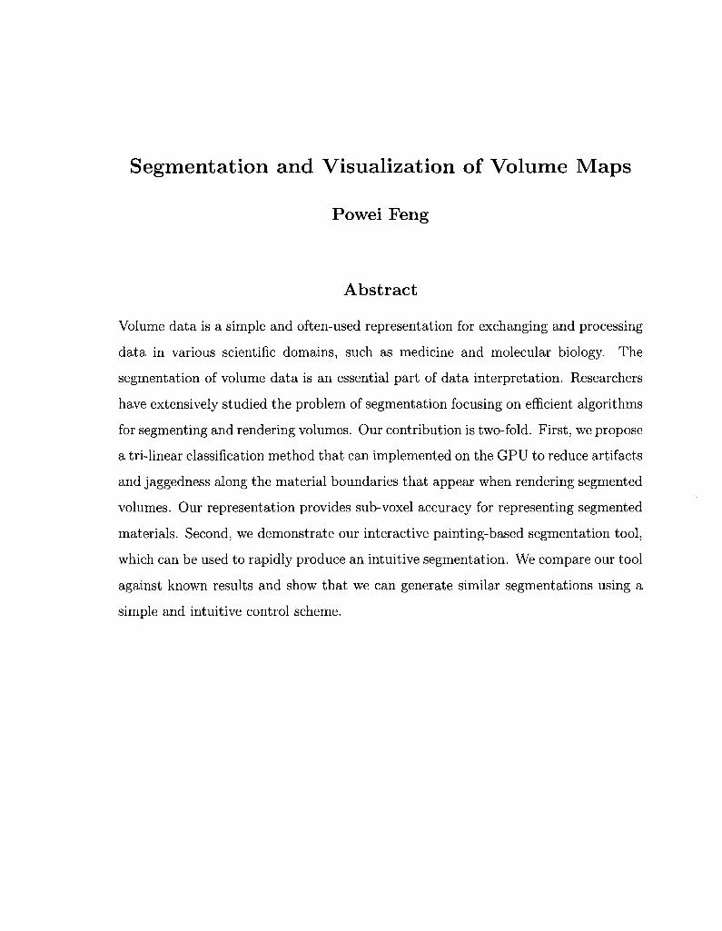
Abstract

Volume data is a simple and often-used representation for exchanging and processing

data in various scientific domains, such as medicine and molecular biology. The

segmentation of volume data is an essential part of data interpretation. Researchers

have extensively studied the problem of segmentation focusing on efficient algorithms

for segmenting and rendering volumes. Our contribution is two-fold. First, we propose

a tri-linear classification method that can implemented on the GPU to reduce artifacts

and jaggedness along the material boundaries that appear when rendering segmented

volumes. Our representation provides sub-voxel accuracy for representing segmented

materials. Second, we demonstrate our interactive painting-based segmentation tool,

which can be used to rapidly produce an intuitive segmentation. We compare our tool

against known results and show that we can generate similar segmentations using a

simple and intuitive control scheme.

11

Acknowledgements

I would like to thank Joe Warren, my advisor, not only for introducing the problem

to me but also for providing careful guidance throughout this research. I would also

like to thank Ron Goldman for detailed comments on how to improve this thesis. I

also thank Luay Nakhleh for serving as part of my committee and imparting helpful

suggestions during the defense.

Contents

Abstract i

List of Illustrations v

1 Introduction 1

1.1 Visualizing Volume Data 2

1.2 Volume Segmentation 6

2 Tri-linear Representation of Segmented Volumes 10

2.1 Multi-material Contouring 10

2.1.1 Classification method 10

2.1.2 Characterization of the Contours 13

2.2 Set Operations on Multi-material Contours 15

2.2.1 Operations on Two Materials 15

2.2.2 Operations for Three or More Materials 17

2.3 Results 18

3 Applications using Tri-linear Contours 20

3.1 Building Scalars from Existing Segmentation 20

3.2 Importing Iso-surfaces 21

3.3 Tri-linear contours with Interactive Segmentation 23

3.4 GPU-implementation 24

4 Painting-based Segmentation 26

4.1 Segmentation with Graph-cut 27

IV

4.2 Results 28

4.2.1 Heterogenous Examples 29

4.2.2 Protein Data Bank Examples 30

5 Conclusion 32

Bibliography 33

Illustrations

1.1 2D example of segmented volume visualization. 1.1(a) shows the

input segmented volume, and 1.1(b) renders a piecewise bi-linear

function over the segmented domain. Note that the bi-linear

classification produces smoother boundary but also maintains the

correct partition. 1.1(c) and 1.1(d) are the three material variants. . 3

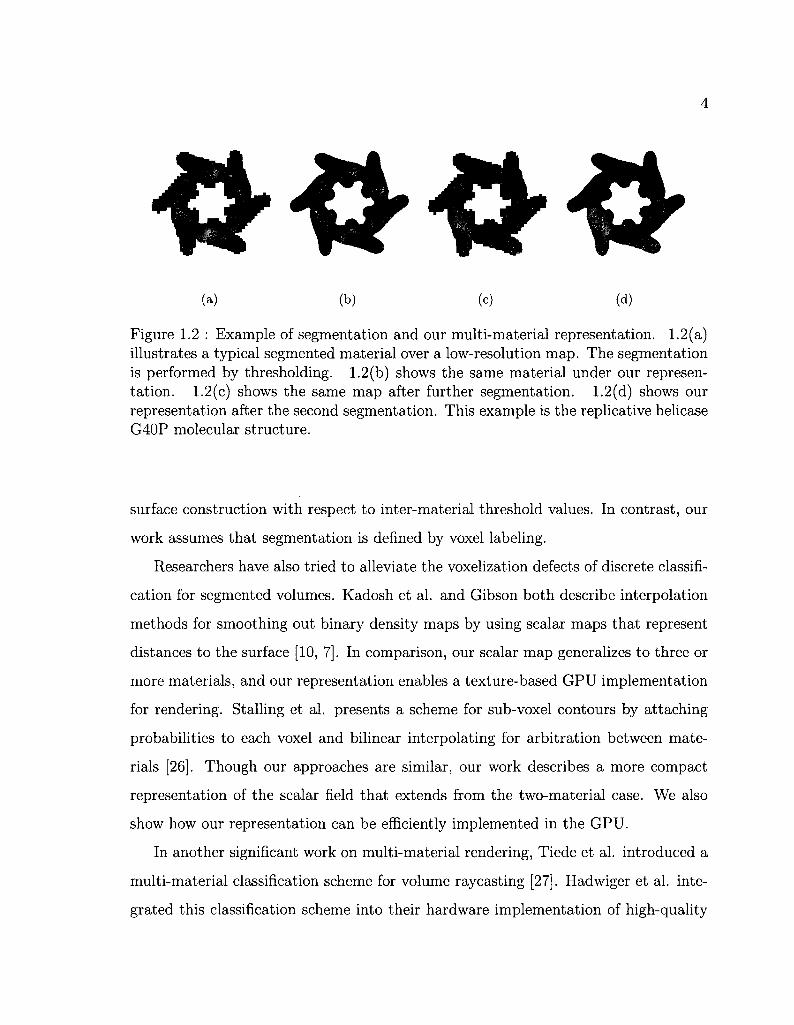
1.2 Example of segmentation and our multi-material representation.

1.2(a) illustrates a typical segmented material over a low-resolution

map. The segmentation is performed by thresholding. 1.2(b) shows

the same material under our representation. 1.2(c) shows the same

map after further segmentation. 1.2(d) shows our representation

after the second segmentation. This example is the replicative

helicase G40P molecular structure 4

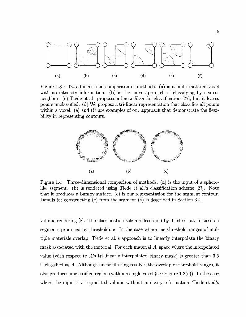
1.3 Two-dimensional comparison of methods, (a) is a multi-material

voxel with no intensity information, (b) is the naive approach of

classifying by nearest neighbor, (c) Tiede et al. proposes a linear

filter for classification [27], but it leaves points unclassified, (d) We

propose a tri-linear representation that classifies all points within a

voxel, (e) and (f) are examples of our approach that demonstrate the

flexibility in representing contours 5

VI

1.4 Three-dimensional comparison of methods, (a) is the input of a

sphere-like segment, (b) is rendered using Tiede et al.'s classification

scheme [27]. Note that it produces a bumpy surface, (c) is our

representation for the segment contour. Details for constructing (c)

from the segment (a) is described in Section 3.4 5

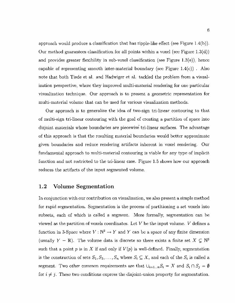
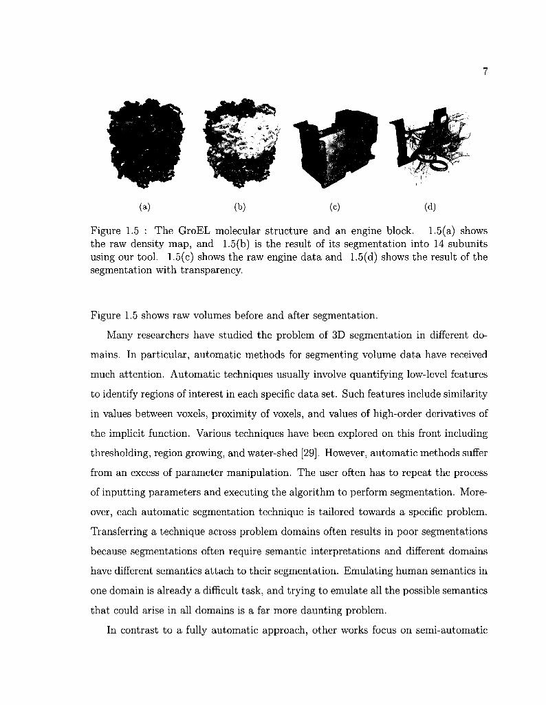
1.5 The GroEL molecular structure and an engine block. 1.5(a) shows

the raw density map, and 1.5(b) is the result of its segmentation into

14 subunits using our tool. 1.5(c) shows the raw engine data and

1.5(d) shows the result of the segmentation with transparency. . . . 7

2.1 Two material example. 2.1(a) shows the bilinear function of a single

cell. Red represents the parts of the cell that has positive values in

the bilinear evaluation, and green represents the negative values. The

arrows indicate the direction of the gradient. 2.1(b) is the plot of the

bilinear function in 3D with the same color representation 11

2.2 2 material example continued. 2.2(a) is the plot of the function in

2.1 by replacing the negative voxels (coefficients of the bilinear) with

O's. 2.2(b) is the plot of the same function by replacing the positive

voxels with O's and taking the absolute value of the coefficients.

2.2(c) is the maximum of the functions in 2.2(a) and 2.2(b) 12

2.3 3 material example. 2.3(a) is the classification of the bi-linear

function under our scheme. The arrows denote the gradient. 2.3(b)

is the plot of 3 functions that are created under our evaluation

scheme. 2.3(c) is the maximum plot of the three functions 12

2.4 The perspective view of a multi-material volume of size 333 rendered

using GPU tri-linear contouring (a) and as polygonal contours

generated by Dual Contouring (b), showing the grid structure (c). (d)

depicts the mesh generated from Dual Contouring without the letters. 15

Vll

2.5 A close up example of rendering using our piecewise tri-linear

representation 19

2.6 A close up example of rendering using our piecewise tri-linear

representation 19

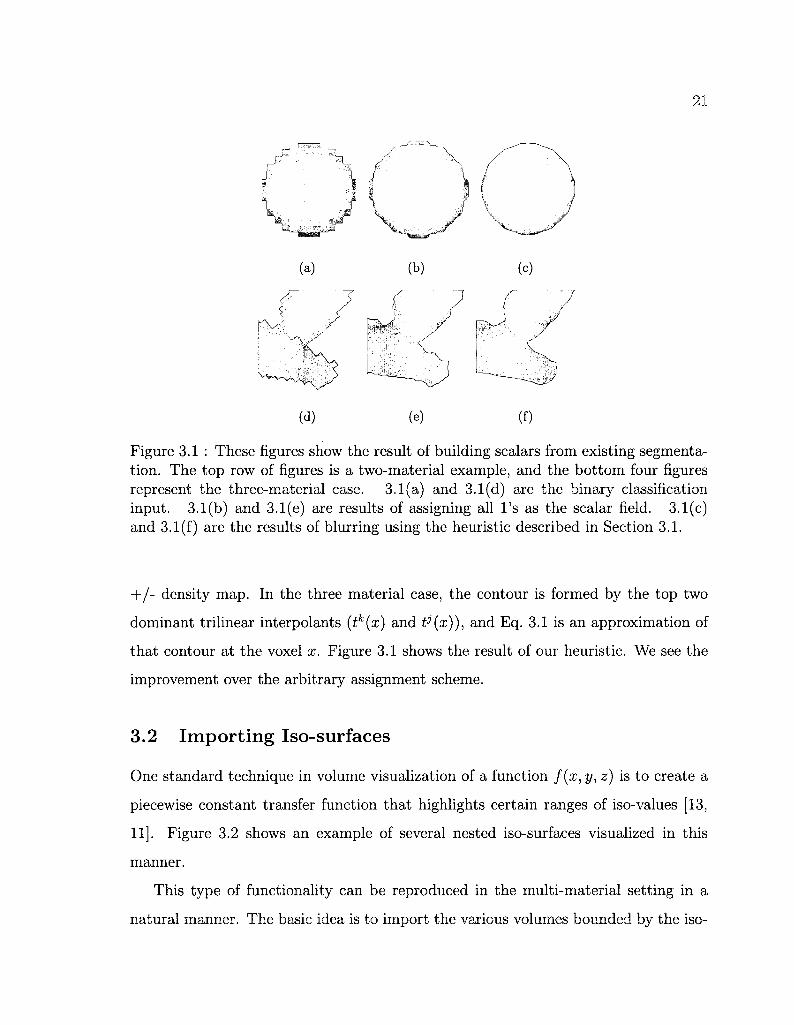
3.1 These figures show the result of building scalars from existing

segmentation. The top row of figures is a two-material example, and

the bottom four figures represent the three-material case. 3.1(a)

and 3.1(d) are the binary classification input. 3.1(b) and 3.1(e) are

results of assigning all l's as the scalar field. 3.1(c) and 3.1(f) are the

results of blurring using the heuristic described in Section 3.1 21

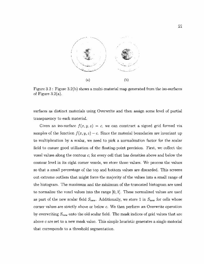
3.2 Figure 3.2(b) shows a multi-material map generated from the

iso-surfaces of Figure 3.2(a) 22

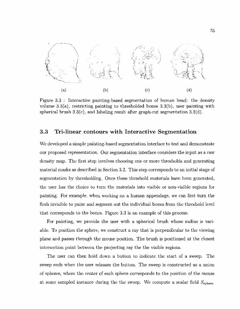
3.3 Interactive painting-based segmentation of human head: the density

volume 3.3(a), restricting painting to thresholded bones 3.3(b), user

painting with spherical brush 3.3(c), and labeling result after

graph-cut segmentation 3.3(d) 23

4.1 PDB examples segmented using our painting interface. In order of

left-to-right, the images of first row are of datasets 1E08 and 1R8J.

The second row images are of 1XTC and 2P1P 31

2 Gallery of examples segmented using our painting interface. In the

order of left-to-right, the figures of the first row are: myosin V

(EMDB 1201), and Hsp 26 (EMDB 1226), glutamate synthase

1.2-MDa hexamer (EMDB 1440), and engine block (General Electric

and volvis.org). The figures of the second row are: Stanford bunny

(The Volume Library), foot (Philips Research and The Volume

Library), Ambystoma Tigrinum (Digital Morphology Library), and

piggy bank (Michael Bauer and The Volume Library)

1

Chapter 1

Introduction

Volume data is defined by a three-dimensional grid of scalar values or tuples. Each

point on the grid is called a voxel. (The two-dimensional version of volume data

is a grey-scale or colored image). Volume data can be generated for simulations

or generated through imaging technology such as computed tomography (CT) in

medicine and electron microscopy (EM) in bio-molecular imaging. The most intuitive

analysis of a 3D volume map is through visualizing the data. For example, given a CT

scan of a hand, we can reconstruct a 3D model of the hand that allows for interactive

visual manipulation such as rotation, translation, and magnification. In addition to

visualizing the entire volume, sometimes it is useful to visualize the components that

reside within a volume map. (In the case of the hand CT, it would be useful if we can

separate out the bones from the flesh). To visualize components within a volume, the

first step is to separate out regions of interest within the data set. This separation

is called segmentation. Besides bone/flesh separation in medicine, segmentation also

corresponds to other high-level semantics such as locating symmetric subunits from a

reconstructed image of a protein (see Figure 1.5(b)) and identifying individual parts

of a mechanical object like an engine (see Figure 1.5(d)).

Our work addresses the specific problem of visualizing segmented volumes. We

focus on reducing the jagged boundary associated with binary classification of seg­

mented volumes. In addition to visualization, we also develop a semi-automatic seg­

mentation interface and demonstrate that this interface is an intuitive and efficient

method for segmentation.

In the rest of this chapter, we will discuss the background and motivation of our

2

work on volume visualization and segmentation. We will also briefly describe our

approach, which is elaborated in the following chapters.

1.1 Visualizing Volume Data

Visualizing volume data requires interpreting the discretely-sampled volume as a con­

tinuous function. One approach is to interpret the space between samples as a tri-

linear interpolation function by treating the discrete samples as the interpolant at the

corners of the function domain. The entire domain of the volume is then covered by

piece-wise tri-linear functions. To display the function defined on the volume, we can

choose a threshold value and extract a level-set from the combined function. This

approach is a form of implicit modeling, which is a standard technique for modeling

shapes in computer graphics [1]. Given a function f(x,y,z) (our previously defined

volume function), the set of all points such that f(x,y, z) < 0 defines the one region

and the set of all points such that f(x,y,z,) > 0 defines a second, complementary

region (excluding the surface where the function is zero). For a multiple material

viewpoint, the implicit function f(x,y,z) partitions space into two materials; one

material where the function f(x, y, z) is positive and another where f(x, y, z) is nega­

tive. Numerous contouring method such as Marching Cubes [15], Dual Contouring [9]

and others [5, 12, 20] can then generate a polygonal surface that separates the positive

space from negative space.

Alternatively, the two spaces can be visualized using various volumetric approaches

implemented on the GPU [28, 4, 22]. The key ideas behind these approaches are that

the signed grid can be stored as a 3D texture and that a single texture load can be

used to evaluate f(x,y,z) via tri-linear interpolation at an arbitrary point. In prac­

tice, this tri-linear boundary surface provides better normals for shading and better

silhouettes than the discrete voxelized approach.

While the use of two signs to distinguish between two materials is simple and

elegant, the idea of using three or more signs to represent a partition of space into

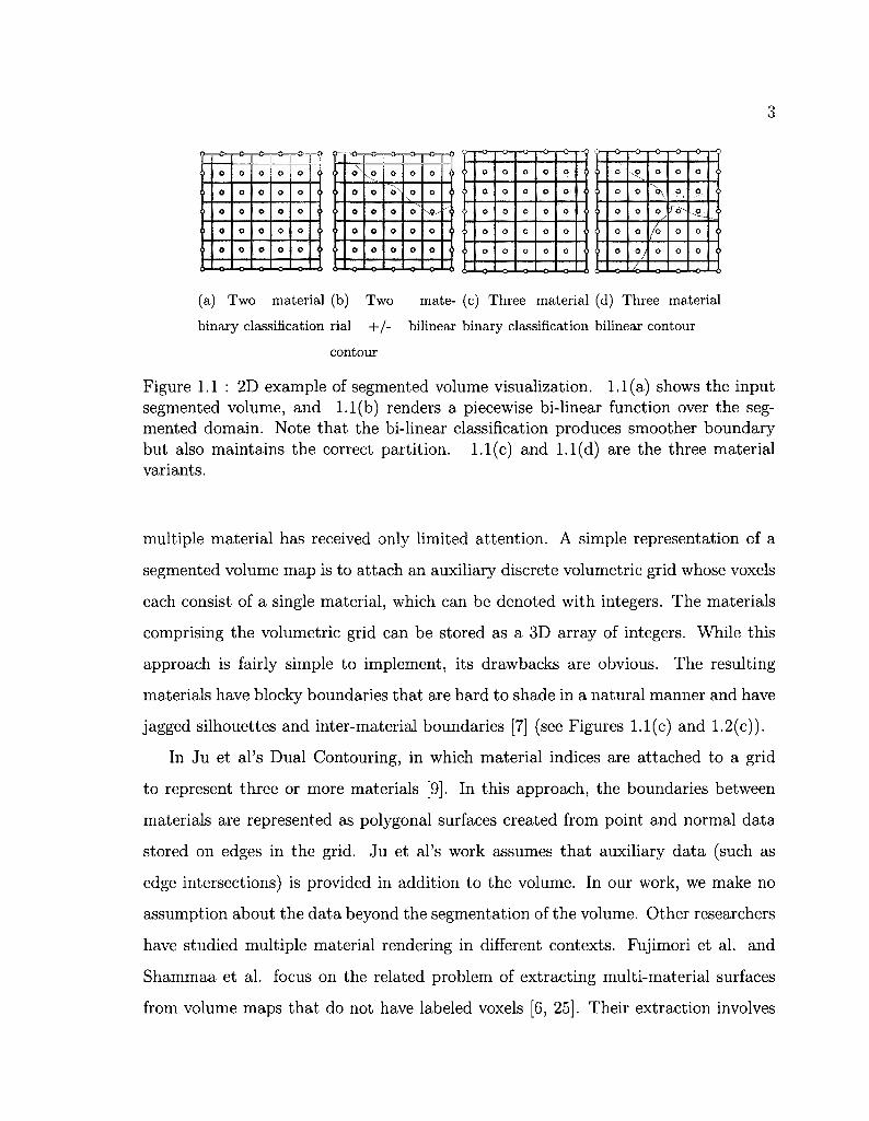
(a) Two material (b) Two mate- (c) Three material (d) Three material

binary classification rial + / - bilinear binary classification bilinear contour

contour

Figure 1.1 : 2D example of segmented volume visualization. 1.1(a) shows the input segmented volume, and 1.1(b) renders a piecewise bi-linear function over the seg­mented domain. Note that the bi-linear classification produces smoother boundary but also maintains the correct partition, 1.1(c) and 1.1(d) are the three material variants.

multiple material has received only limited attention. A simple representation of a

segmented volume map is to attach an auxiliary discrete volumetric grid whose voxels

each consist of a single material, which can be denoted with integers. The materials

comprising the volumetric grid can be stored as a 3D array of integers. While this

approach is fairly simple to implement, its drawbacks are obvious. The resulting

materials have blocky boundaries that are hard to shade in a natural manner and have

jagged silhouettes and inter-material boundaries [7] (see Figures 1.1(c) and 1.2(c)).

In Ju et al's Dual Contouring, in which material indices are attached to a grid

to represent three or more materials [9]. In this approach, the boundaries between

materials are represented as polygonal surfaces created from point and normal data

stored on edges in the grid. Ju et al's work assumes that auxiliary data (such as

edge intersections) is provided in addition to the volume. In our work, we make no

assumption about the data beyond the segmentation of the volume. Other researchers

have studied multiple material rendering in different contexts. Fujimori et al. and

Shammaa et al. focus on the related problem of extracting multi-material surfaces

from volume maps that do not have labeled voxels [6, 25]. Their extraction involves

4

(a) (b) (c) (d)

Figure 1.2 : Example of segmentation and our multi-material representation. 1.2(a) illustrates a typical segmented material over a low-resolution map. The segmentation is performed by thresholding. 1.2(b) shows the same material under our represen­tation. 1.2(c) shows the same map after further segmentation. 1.2(d) shows our representation after the second segmentation. This example is the replicative helicase G40P molecular structure.

surface construction with respect to inter-material threshold values. In contrast, our

work assumes that segmentation is defined by voxel labeling.

Researchers have also tried to alleviate the voxelization defects of discrete classifi­

cation for segmented volumes. Kadosh et al. and Gibson both describe interpolation

methods for smoothing out binary density maps by using scalar maps that represent

distances to the surface [10, 7]. In comparison, our scalar map generalizes to three or

more materials, and our representation enables a texture-based GPU implementation

for rendering. Stalling et al. presents a scheme for sub-voxel contours by attaching

probabilities to each voxel and bilinear interpolating for arbitration between mate­

rials [26]. Though our approaches are similar, our work describes a more compact

representation of the scalar field that extends from the two-material case. We also

show how our representation can be efficiently implemented in the GPU.

In another significant work on multi-material rendering, Tiede et al. introduced a

multi-material classification scheme for volume raycasting [27]. Hadwiger et al. inte­

grated this classification scheme into their hardware implementation of high-quality

9

oo

QQ

00

9 9~r^? 9^r^? 9 = ^

00 oo CO 0) (a) (b) (c) (d) (e) (f)

Figure 1.3 : Two-dimensional comparison of methods, (a) is a multi-material voxel with no intensity information, (b) is the naive approach of classifying by nearest neighbor, (c) Tiede et al. proposes a linear filter for classification [27], but it leaves points unclassified, (d) We propose a tri-linear representation that classifies all points within a voxel, (e) and (f) are examples of our approach that demonstrate the flexi­bility in representing contours.

(a) (b) (c)

Figure 1.4 : Three-dimensional comparison of methods, (a) is the input of a sphere­like segment, (b) is rendered using Tiede et al.'s classification scheme [27]. Note that it produces a bumpy surface, (c) is our representation for the segment contour. Details for constructing (c) from the segment (a) is described in Section 3.4.

volume rendering [8]. The classification scheme described by Tiede et al. focuses on

segments produced by thresholding. In the case where the threshold ranges of mul­

tiple materials overlap, Tiede et al.'s approach is to linearly interpolate the binary

mask associated with the material. For each material A, space where the interpolated

value (with respect to A's tri-linearly interpolated binary mask) is greater than 0.5

is classified as A. Although linear filtering resolves the overlap of threshold ranges, it

also produces unclassified regions within a single voxel (see Figure 1.3(c)). In the case

where the input is a segmented volume without intensity information, Tiede et al's

6

approach would produce a classification that has ripple-like effect (see Figure 1.4(b)).

Our method guarantees classification for all points within a voxel (see Figure 1.3(d))

and provides greater flexibility in sub-voxel classification (see Figure 1.3(e)), hence

capable of representing smooth inter-material boundary (see Figure 1.4(c)) . Also

note that both Tiede et al. and Hadwiger et al. tackled the problem from a visual­

ization perspective, where they improved multi-material rendering for one particular

visualization technique. Our approach is to present a geometric representation for

multi-material volume that can be used for various visualization methods.

Our approach is to generalize the idea of two-sign tri-linear contouring to that

of multi-sign tri-linear contouring with the goal of creating a partition of space into

disjoint materials whose boundaries are piecewise tri-linear surfaces. The advantage

of this approach is that the resulting material boundaries would better approximate

given boundaries and reduce rendering artifacts inherent in voxel rendering. Our

fundamental approach to multi-material contouring is viable for any type of implicit

function and not restricted to the tri-linear case. Figure 1.5 shows how our approach

reduces the artifacts of the input segmented volume.

1.2 Volume Segmentation

In conjunction with our contribution on visualization, we also present a simple method

for rapid segmentation. Segmentation is the process of partitioning a set voxels into

subsets, each of which is called a segment. More formally, segmentation can be

viewed as the partition of voxels coordinates. Let V be the input volume. V defines a

function in 3-Space where V : N3 —> Y and Y can be a space of any finite dimension

(usually Y = R). The volume data is discrete so there exists a finite set X C N3

such that a point p is in X if and only if V{p) is well-defined. Finally, segmentation

is the construction of sets S\, S2, • • •, Sn where Si C X, and each of the Si is called a

segment. Two other common requirements are that l)i=i...nSi = X and Si fl Sj = 0

for i ^ j . These two conditions express the disjoint-union property for segmentation.

7

(a) (b) (c) (d)

Figure 1.5 : The GroEL molecular structure and an engine block. 1.5(a) shows the raw density map, and 1.5(b) is the result of its segmentation into 14 subunits using our tool. 1.5(c) shows the raw engine data and 1.5(d) shows the result of the segmentation with transparency.

Figure 1.5 shows raw volumes before and after segmentation.

Many researchers have studied the problem of 3D segmentation in different do­

mains. In particular, automatic methods for segmenting volume data have received

much attention. Automatic techniques usually involve quantifying low-level features

to identify regions of interest in each specific data set. Such features include similarity

in values between voxels, proximity of voxels, and values of high-order derivatives of

the implicit function. Various techniques have been explored on this front including

thresholding, region growing, and water-shed [29]. However, automatic methods suffer

from an excess of parameter manipulation. The user often has to repeat the process

of inputting parameters and executing the algorithm to perform segmentation. More­

over, each automatic segmentation technique is tailored towards a specific problem.

Transferring a technique across problem domains often results in poor segmentations

because segmentations often require semantic interpretations and different domains

have different semantics attach to their segmentation. Emulating human semantics in

one domain is already a difficult task, and trying to emulate all the possible semantics

that could arise in all domains is a far more daunting problem.

In contrast to a fully automatic approach, other works focus on semi-automatic

8

methods that require some level of user input. These methods provide more accuracy

and more control over automatic methods. Work in this area involves using an input

device (i.e. the mouse) and marking the segments manually. Given enough user

input, automatic techniques can then be applied to the volume with greater accuracy.

The additional input from the user helps guide the automatic process, and using

automation prevents the user from manually marking the entire volume, which can

be an error-prone and time consuming process.

Previous works on semi-automatic methods include Owada et al.'s Volume Catcher

and Yuan et al.'s Volume Cutout [19, 29]. Volume Catcher allows the user to draw

2D free-form strokes on volume; the strokes are then extended using region growing

and set as constraints for graph-based segmentation. Volume Cutout uses two kinds

of strokes to denote the foreground and the background on a two-dimensional view

of the 3D volume. The strokes are then used in a graph-based approach to automate

the segmentation for the rest of the volume. These two approaches both focus on

the problem of two-material segmentation. We are interested in generalized, multi-

material segmentation.

Another difficulty in semi-automatic segmentation is in manipulating 3D objects

using a 2D interface. Many of the existing methods involve extending 2D segmen­

tation techniques by applying segmentation to 2D slices and re-constructing the 3D

segmentation. However, it is hard to identify 3D spatial correlation and features using

this approach. We choose an approach that operates directly on the 3D volume with

semi-automated segmentation using graph-cut. Graph-cut methods have proven to

be useful for segmenting 2D images. Typically, 2D graph-cuts involve denoting the

foreground and background of the graph/image through user input and performing

a min-cut/max-flow variant to identify two sets of nodes/pixels. The min-cut in­

duces a natural component partition across the image that satisfies the criterion of

segmentation. The 3D complement of this approach has been used by Liu et al. for

bone segmentation [14]. Their work takes the rectilinear grid as the graph for the

9

cut. Seeds are placed by the user on 2D slices to perform segmentation. We build

upon their method, using a 3D interface and complementing the process with hard­

ware rendering that allows for interactive visualization and editing of volume data

sets. Our tool lets the user partially paint the desired segmentation and fill in the

unpainted portions by applying the graph-cut optimization.

The following chapters will be organized as the following: Chapter 2 will present

the details of our visualization representation for segmented volumes; Chapter 3 will

cover how our representation can be applied in practical settings; Chapter 4 will

discuss our painting-based segmentation interface and present the results.

10

Chapter 2

Tri-linear Representation of Segmented Volumes

2.1 Multi-material Contouring

2.1.1 Classification method

Our approach for multi-material contouring is to replace a signed grid of scalars with

a grid whose vertices have an associated scalar and material. In the two material

case, our method should reproduce the standard +/— interpretation using normal

contouring. In the case of three or more materials, the contouring method should

generate piecewise tri-linear contours that join continuously along the faces of the

grid.

Given a grid cell whose corners have associated non-negative scalars Sj and ma­

terial indices m,, the following method can be used to determine the material index

of a point x inside the cell. The index i ranges from 0 to 7, representing the eight

corners of a cell.

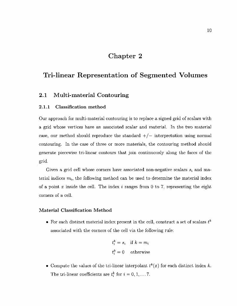
Material Classification Method

• For each distinct material index present in the cell, construct a set of scalars tk

associated with the corners of the cell via the following rule:

tk — Si if k = rrii

tk = 0 otherwise

• Compute the values of the tri-linear interpolant tk{x) for each distinct index k.

The tri-linear coefficients are tk for i = 0 , 1 , . . . 7.

11

(a) (b)

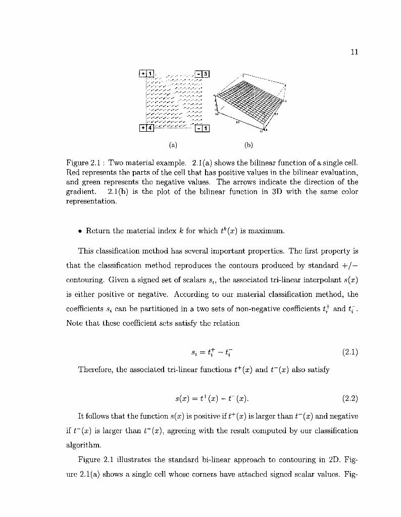
Figure 2.1 : Two material example. 2.1(a) shows the bilinear function of a single cell. Red represents the parts of the cell that has positive values in the bilinear evaluation, and green represents the negative values. The arrows indicate the direction of the gradient. 2.1(b) is the plot of the bilinear function in 3D with the same color representation.

• Return the material index k for which tk(x) is maximum.

This classification method has several important properties. The first property is

that the classification method reproduces the contours produced by standard +/—

contouring. Given a signed set of scalars S;, the associated tri-linear interpolant s(x)

is either positive or negative. According to our material classification method, the

coefficients Sj can be partitioned in a two sets of non-negative coefficients tf and t~.

Note that these coefficient sets satisfy the relation

sl = tt-t~ (2.1)

Therefore, the associated tri-linear functions t+(x) and t~(x) also satisfy

s(x) =t+{x)-r(x). (2.2)

It follows that the function s(x) is positive if t+(x) is larger than t~(x) and negative

if t~(x) is larger than t+(x), agreeing with the result computed by our classification

algorithm.

Figure 2.1 illustrates the standard bi-linear approach to contouring in 2D. Fig­

ure 2.1(a) shows a single cell whose corners have attached signed scalar values. Fig-

12

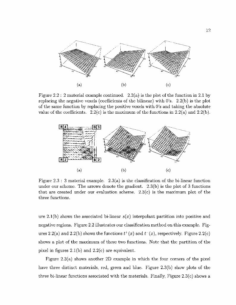
(a) (b) (c)

Figure 2.2 : 2 material example continued. 2.2(a) is the plot of the function in 2.1 by replacing the negative voxels (coefficients of the bilinear) with O's. 2.2(b) is the plot of the same function by replacing the positive voxels with O's and taking the absolute value of the coefficients. 2.2(c) is the maximum of the functions in 2.2(a) and 2.2(b).

(a) (b) (c)

Figure 2.3 : 3 material example. 2.3(a) is the classification of the bi-linear function under our scheme. The arrows denote the gradient. 2.3(b) is the plot of 3 functions that are created under our evaluation scheme. 2.3(c) is the maximum plot of the three functions.

ure 2.1(b) shows the associated bi-linear s(x) interpolant partition into positive and

negative regions. Figure 2.2 illustrates our classification method on this example. Fig­

ures 2.2(a) and 2.2(b) shows the functions t+(x) and t~(x), respectively. Figure 2.2(c)

shows a plot of the maximum of these two functions. Note that the partition of the

pixel in figures 2.1(b) and 2.2(c) are equivalent.

Figure 2.3(a) shows another 2D example in which the four corners of the pixel

have three distinct materials, red, green and blue. Figure 2.3(b) show plots of the

three bi-linear functions associated with the materials. Finally, Figure 2.3(c) shows a

13

plot of the maximum of these functions and the associated partition of the pixels into

three distinct materials via three bi-linear contours that meet at a common point.

2.1.2 Characterization of the Contours

The multi-material contours produced by this method have several important prop­

erties. First, the contours are continuous across cells sharing a common face. This

fact follows from the observation that two cells sharing a common face have the same

scalars and material indices on that face. Since the restriction of the tri-linear func­

tions used in defining the multi-material contour on this face depend only on the

scalar and material indices on that face, the multi-material contours must agree.

Piecewise Tri-linear Surfaces

Inside a single cell, the resulting contours are simply piecewise contours of various

tri-linear functions. To understand why, note that the contours bounding the region

associated with a material with index k are simply surfaces where the tri-linear func­

tion th(x) and another tri-linear function tj(x) both reach the maximum. Therefore,

this contour is an iso-surface of the form

tk(x)=tj(x)

We have used a GPU-based, volume rendering approach to find the contour in

our implementation. However, it is possible to solve this classification problem using

polygonal methods such as Dual Contouring. Under Dual Contouring, we find a

point within the cell that best describes the intersection of all the pairwise tri-linear

surfaces. More formally, let M be the set of materials within a cell and let x be a

point inside the cell. Consider the function

E(x)= £ {tk{x)-V{x)Y (2.3) j,k€M,jjtk

14

The minimum of this function describes a point that is closest to the intersection of all

the surfaces that satisfy tk(x) = tj(x). This is a non-linear optimization problem that

can be costly to compute. We approximate the solution using an QEF-based approach

that is described by Schaefer et al [24], This method locates the intersections, p^, of

the surfaces along the cell edges. These intersections and the normals, r^, at these

points describe a set of planes per cell. We then find a point that minimizes

E'{x) = Y,{n%-{x-Pl)f (2.4) i

This minimization gives an approximation of Eq. 2.3 that is reasonable for our pur­

pose. Note that this is an outline for computing the contour point. Please refer to

the work of Schaefer et al. for more implementation details [24].

Since we are replacing the tri-linear function in each cell with linear approxima­

tions, the contour may not retain enough details of the original function. We can

retrieve these details by subdividing the grid space into finer cells. The new mask in­

dices are determined by the classification method described previously; the new scalar

for the refined map must be computed per each material. In effect, this approach will

expand the storage size for the scalar by a factor of n, where n is the number of ma­

terials. This can be done adaptively to subdivide cells only along material border to

reduce the computation and storage size. In our experiments, we perform a uniform

subdivision over the entire volume, but we also notice that refinement is not necessary

in most cases. Figure 2.4 shows the results of meshing using Dual Contouring.

Gradient

One useful property from standard implicit modeling is that the gradient of the

implicit function is normal to the contours of that function. In the multi-material case,

a similar property holds. Given a contour formed by the iso-surface tk(x) = P(x), the

gradient of the function tk(x) — P(x) is simply the normal to this surface. The key

observation here is that the pair of material indices j and k change as the point x varies

15

(a) (b) (c) (d)

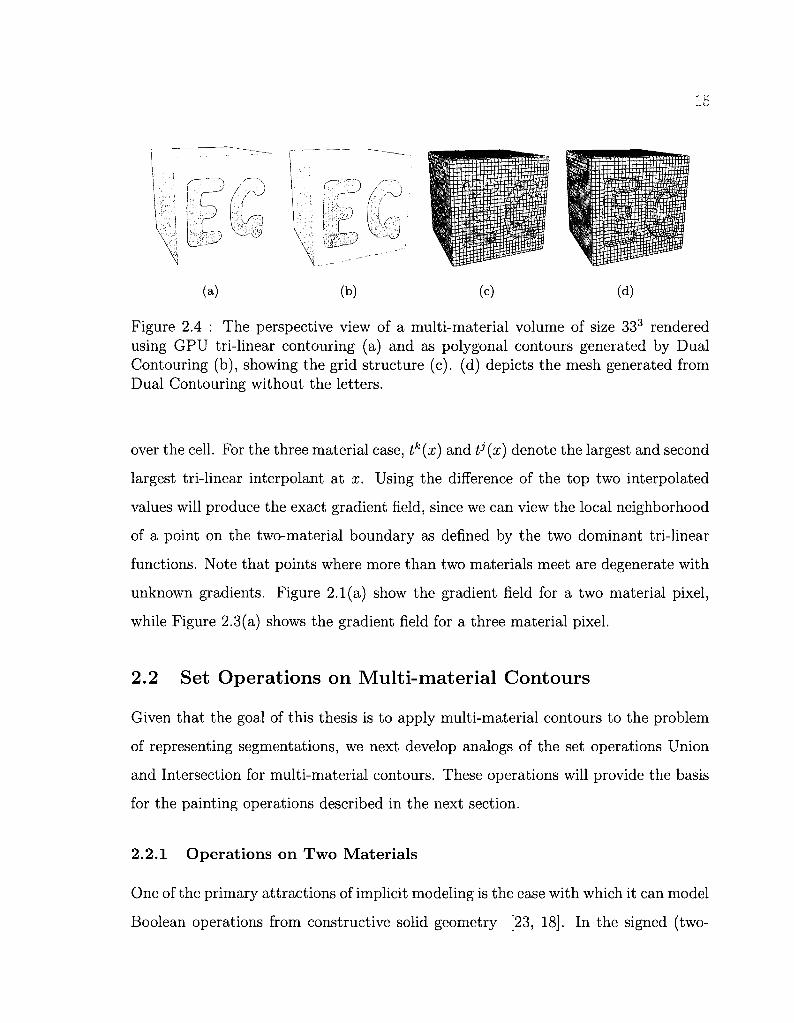
Figure 2.4 : The perspective view of a multi-material volume of size 333 rendered using GPU tri-linear contouring (a) and as polygonal contours generated by Dual Contouring (b), showing the grid structure (c). (d) depicts the mesh generated from Dual Contouring without the letters.

over the cell. For the three material case, tk(x) and P(x) denote the largest and second

largest tri-linear interpolant at x. Using the difference of the top two interpolated

values will produce the exact gradient field, since we can view the local neighborhood

of a point on the two-material boundary as defined by the two dominant tri-linear

functions. Note that points where more than two materials meet are degenerate with

unknown gradients. Figure 2.1(a) show the gradient field for a two material pixel,

while Figure 2.3(a) shows the gradient field for a three material pixel.

2.2 Set Operations on Multi-material Contours

Given that the goal of this thesis is to apply multi-material contours to the problem

of representing segmentations, we next develop analogs of the set operations Union

and Intersection for multi-material contours. These operations will provide the basis

for the painting operations described in the next section.

2.2.1 Operations on Two Materials

One of the primary attractions of implicit modeling is the ease with which it can model

Boolean operations from constructive solid geometry [23, 18]. In the signed (two-

16

material) case, the typical convention is to represent a solid as the set of solutions to

the inequality f(x, y, z) < 0. Now, given two solids f(x, y, z) < 0 and g(x, y, z) < 0,

the union of these two solids is simply the set min(/(x, y, z),g(x, y, z)) < 0 while the

intersection of two solids is the set max(/(x, y, z),g(x, y, z)) < 0.

If the functions / and g are represented by signed grids, a standard technique

for approximating their union or intersection is to take the min or max of their

associated sign grids. Our goal is to develop equivalent rules for the two-material

case that generalize to the multi-material case in a natural manner.

Our approach is as follows; consider two materials A and ->A (not A). A can be

interpreted as being the inside of a solid (i.e; negative in the implicit model) and ->A

can be interpreted as being the outside of a solid (i.e; positive in the implicit model.).

Given a multi-material map consist of only these two materials, we can attempt to

construct rules for computing new non-negative scalars and material indices on the

grid that reproduce the operations Union and Intersection.

In particular, give a grid point with two associated pairs (s\, kx) and (s2, k2) (where

both the Si are non-negative), our goal is to compute a scalar/index pair (s,k) for

the union of the material S. This new pair can be computed using the following case

look-up given in Table 2.1.

Note that the rule for computing k is straightforward. For Union, the new material

index is A if and only if at least one of the material indices is A. For Intersection, the

new material index is A if and only if both of the material indices are A. The rule for

computing the new scalar s is only slightly more involved. The key is converted back

to the signed case and then return the result of taking the min of the converted scalars.

For example, if both material indices are A, we take the negative of both scalars S\

and s2, compute their min and then negate the result. These three operations are

simply the equivalent of taking the max of the original scalars. In particular, if both

Si and s2 are non-negative,

max(si, s2) = — min(—Si, —s2) (2.5)

17

Union

fci

A

A

-^A

-^A

k2

A

-^A

A

^A

k

A

A

A

-^A

s

max(si,s2)

S\

s2

min(si,s2)

Intersection

fci

A

A

-u4

^A

k2

A

-^A

A

-IA

k

A

^A

-IA

^A

s

min(si,s2)

«2

S\

max(si,s2)

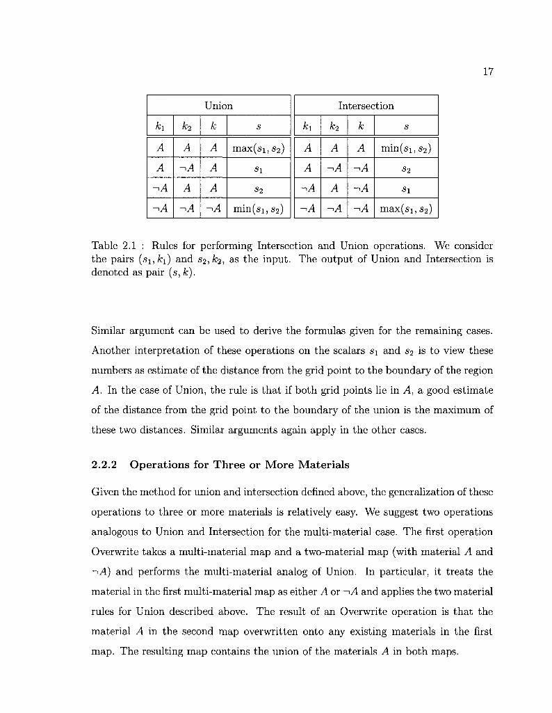
Table 2.1 : Rules for performing Intersection and Union operations. We consider the pairs (si,fci) and s2,&2, as the input. The output of Union and Intersection is denoted as pair (s, k).

Similar argument can be used to derive the formulas given for the remaining cases.

Another interpretation of these operations on the scalars si and s2 is to view these

numbers as estimate of the distance from the grid point to the boundary of the region

A. In the case of Union, the rule is that if both grid points lie in A, a good estimate

of the distance from the grid point to the boundary of the union is the maximum of

these two distances. Similar arguments again apply in the other cases.

2.2.2 Operations for Three or More Materials

Given the method for union and intersection defined above, the generalization of these

operations to three or more materials is relatively easy. We suggest two operations

analogous to Union and Intersection for the multi-material case. The first operation

Overwrite takes a multi-material map and a two-material map (with material A and

-iA) and performs the multi-material analog of Union. In particular, it treats the

material in the first multi-material map as either A or -<A and applies the two material

rules for Union described above. The result of an Overwrite operation is that the

material A in the second map overwritten onto any existing materials in the first

map. The resulting map contains the union of the materials A in both maps.

18

model

engine

foot

head

GroEL

size

256 x 256 x 256

256 x 256 x 256

128 x 256 x 256

240 x 240 x 240

basic (fps)

34

37

40

38

classify (fps)

14

10

13

16

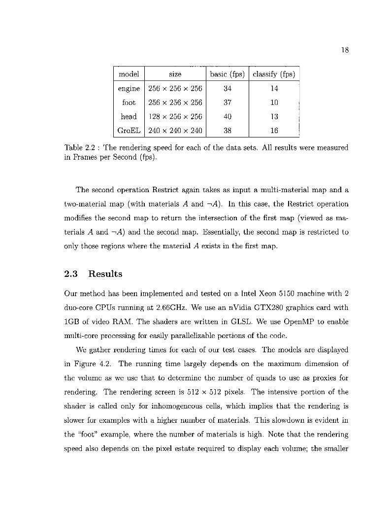
Table 2.2 : The rendering speed for each of the data sets. All results were measured in Frames per Second (fps).

The second operation Restrict again takes as input a multi-material map and a

two-material map (with materials A and ->A). In this case, the Restrict operation

modifies the second map to return the intersection of the first map (viewed as ma­

terials A and ->A) and the second map. Essentially, the second map is restricted to

only those regions where the material A exists in the first map.

2.3 Results

Our method has been implemented and tested on a Intel Xeon 5150 machine with 2

duo-core CPUs running at 2.66GHz. We use an nVidia GTX280 graphics card with

1GB of video RAM. The shaders are written in GLSL. We use OpenMP to enable

multi-core processing for easily parallelizable portions of the code.

We gather rendering times for each of our test cases. The models are displayed

in Figure 4.2. The running time largely depends on the maximum dimension of

the volume as we use that to determine the number of quads to use as proxies for

rendering. The rendering screen is 512 x 512 pixels. The intensive portion of the

shader is called only for inhomogeneous cells, which implies that the rendering is

slower for examples with a higher number of materials. This slowdown is evident in

the "foot" example, where the number of materials is high. Note that the rendering

speed also depends on the pixel estate required to display each volume; the smaller

19

the volume appears on the screen, regardless of Input size, the faster the rendering

will be, which is as expected. Our results are taken from the slowest rendering time

for each of the test sets. Our method maintains a reasonable frame-rate even under

classification.

(a) (b) (c)

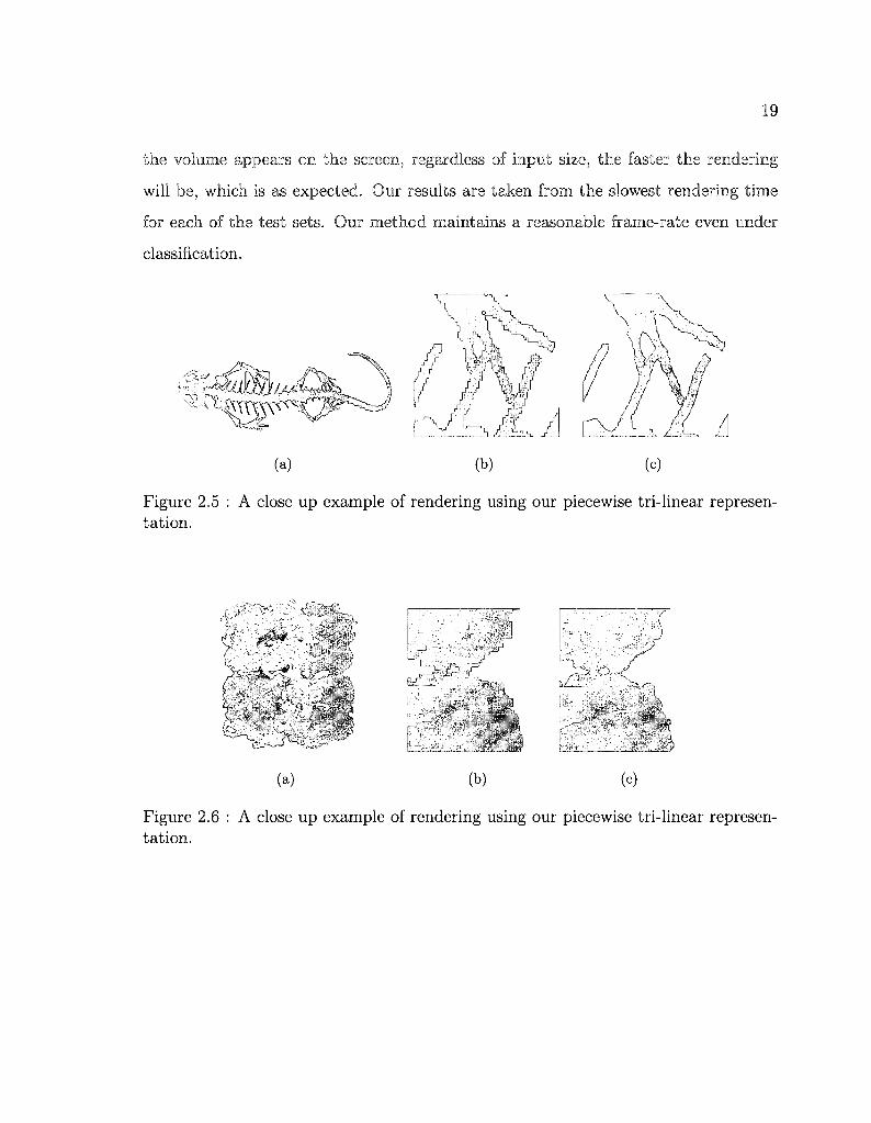
Figure 2.5 : A close up example of rendering using our piecewise tri-linear represen­tation.

(a) (b) (c)

Figure 2.6 : A close up example of rendering using our piecewise tri-linear represen­tation.

20

Chapter 3

Applications using Tri-linear Contours

3.1 Building Scalars from Existing Segmentation

In the case where segmented data are given as input, we present a simple heuristic to

produce scalars off of the binary classification of a typical segmentation. Segmentation

inputs are typically defined by associating an integer value at each voxel or by creating

multiple 0-1 mask volumes, where each one represents a segment. Either of the two

representation can be easily converted to the other. Without loss of generality, we

assume the input is n 0-1 (binary) masks, where each masks represents one of n total

segments.

Under our contour representation, we can an assign arbitrary scalar to each voxel,

and the resulting surface should be a smoother surface than a binary classification.

Unfortunately, this type of assignment does not produce desirable rendering of the

segmented map (see Figures 3.1(b) and 3.1(e)). Instead, we blur each of the binary

masks using a truncated 3 x 3 x 3 gaussian function as our kernel [7]. We can view

the output of the blurring as n scalars defined for each voxel, but the final output we

want is a single scalar defined for each voxel. Using the convention defined previously,

we write the following as the final output scalar, tnew(x), at the voxel x.

tnew(x)=tk(x)-tj{x) (3.1)

where tk(x) and P(x) are the largest and second largest of the n values computed

from the blurring step.

This heuristic is guided by the same intuition given in the gradient discussion of

Section 2.1.2. In the two-material case, the contour will correspond the blurring of a

21

(b) (c)

(d) (e) (f)

Figure 3.1 : These figures show the result of building scalars from existing segmenta­tion. The top row of figures is a two-material example, and the bottom four figures represent the three-material case. 3.1(a) and 3.1(d) are the binary classification input. 3.1(b) and 3.1(e) are results of assigning all l's as the scalar field. 3.1(c) and 3.1(f) are the results of blurring using the heuristic described in Section 3.1.

+ / - density map. In the three material case, the contour is formed by the top two

dominant trilinear interpolants (tk(x) and V(x)), and Eq. 3.1 is an approximation of

that contour at the voxel x. Figure 3.1 shows the result of our heuristic. We see the

improvement over the arbitrary assignment scheme.

3.2 Importing Iso-surfaces

One standard technique in volume visualization of a function f(x, y, z) is to create a

piecewise constant transfer function that highlights certain ranges of iso-values [13,

11], Figure 3.2 shows an example of several nested iso-surfaces visualized in this

manner.

This type of functionality can be reproduced in the multi-material setting in a

natural manner. The basic idea is to import the various volumes bounded by the iso-

22

> * j * i \

(a) (b)

Figure 3.2 : Figure 3.2(b) shows a multi-material map generated from the iso-surfaces of Figure 3.2(a).

surfaces as distinct materials using Overwrite and then assign some level of partial

transparency to each material.

Given an iso-surf ace f(x,y,z) = c, we can construct a signed grid formed via

samples of the function f(x, y, z) — c. Since the material boundaries are invariant up

to multiplication by a scalar, we need to pick a normalization factor for the scalar

field to ensure good utilization of the floating-point precision. First, we collect the

voxel values along the contour c; for every cell that has densities above and below the

contour level in its eight corner voxels, we store those values. We process the values

so that a small percentage of the top and bottom values are discarded. This screens

out extreme outliers that might force the majority of the values into a small range of

the histogram. The maximum and the minimum of the truncated histogram are used

to normalize the voxel values into the range [0,1]. These normalized values are used

as part of the new scalar field Snew. Additionally, we store 1 in Snew for cells whose

corner values are strictly above or below c. We then perform an Overwrite operation

by overwriting Snew onto the old scalar field. The mask indices of grid values that are

above c are set to a new mask value. This simple heuristic generates a single material

that corresponds to a threshold segmentation.

23

(a) (b) (c) (d)

Figure 3.3 : Interactive painting-based segmentation of human head: the density volume 3.3(a), restricting painting to thresholded bones 3.3(b), user painting with spherical brush 3.3(c), and labeling result after graph-cut segmentation 3.3(d).

3.3 Tri-linear contours with Interactive Segmentation

We developed a simple painting-based segmentation interface to test and demonstrate

our proposed representation. Our segmentation interface considers the input as a raw

density map. The first step involves choosing one or more thresholds and generating

material masks as described in Section 3.2. This step corresponds to an initial stage of

segmentation by thresholding. Once these threshold materials have been generated,

the user has the choice to turn the materials into visible or non-visible regions for

painting. For example, when working on a human appendage, we can first turn the

flesh invisible to paint and segment out the individual bones from the threshold level

that corresponds to the bones. Figure 3.3 is an example of this process.

For painting, we provide the user with a spherical brush whose radius is vari­

able. To position the sphere, we construct a ray that is perpendicular to the viewing

plane and passes through the mouse position. The brush is positioned at the closest

intersection point between the projecting ray the the visible regions.

The user can then hold down a button to indicate the start of a sweep. The

sweep ends when the user releases the button. The sweep is constructed as a union

of spheres, where the center of each sphere corresponds to the position of the mouse

at some sampled instance during the the sweep. We compute a scalar field Sphere,

24

using the union of spheres and the computation detailed in Section 3.4. The Sphere

is then restricted to the visible region using the Restrict operation to build a new

field S'new The restriction will enable users to paint only on regions that are visible.

After the restriction, we perform an Overwrite of the old scalar field with the new

field S'new All grid points that lie inside the union of spheres are assigned the mask

index associated with the current brush.

Manual painting can be time-consuming. It is also prone to human error in con­

trolling the painting device. Therefore, we decided to use automatic segmentation to

aid our process. In particular, we find the graph-cut approach of segmentation to be

very effective. We follow the method described by Liu et al. and extend it to a 3D

interface [14]. We will briefly describe this method in the next chapter; please refer

to Liu et al.'s work for more information. The scalars along the new inter-material

boundaries can be computed using our method from Section 3.1 or the distance map

method described by Gibson [7].

3.4 GPU-implementation

We use texture-based volume rendering as our algorithm for visualizing density maps.

All volume maps (i.e. density map, auxiliary scalars, mask, etc.) are stored as 3D

textures [28, 2]. Coloring a single screen fragment involves a number of texture loads

to determine the density, color, and shade of the fragment in texture space. For our

classification algorithm, we need to load an additional 8 scalar values and 8 integers as

part of the fragment shader program. Texture loads are typically expensive operations

in shader programming. However, these 16 loads can be reduced to 4 loads by packing

the values into the RGBA channels for a single texel.

We store both the distance scalars and material masks as 8-bit textures, which

allows up to 256 materials. With only 8-bits of precision for the distance scalars,

we need to ensure that the precision is not wasted on non-essential portions of the

representation. Note that the scalars are used for arbitration only on the border

25

between different materials. This property implies that the scalars need to be accurate

only for cells that intersect the inter-material boundary. We call a cell homogenous if

its eight corners are marked as the same material; otherwise, a cell is inhomogeneous.

For the spherical brush, we use the following distance metric for the new scalar field

g(x, y, z) = \r — \Jx2 + y2 + z2\

if (x, y, z) is part of an inhomogeneous cell (3-2)

g(x,y,z) = l otherwise

Here r is the radius of the brush, and x £ { 0 , 1 , . . . ,nx — 1} denote the grid space

coordinates where nx is the number of grid points in the x direction, and similar

definitions holds for the variables y and z.

From Eq. 3.2 for any grid point (x, y, z) on a inhomogeneous cell, the associated

scalar is bounded by 0 < g(x,y,z) < y/3. Because the Euclidean distance function

ensures that the distance between any two points in a cell cannot exceed y/3. In

contrast, the squared distance function g~(x, y, z) = \r2 — (x2 + y2 + z2)\ does not have

this property; that is, the absolute difference \~g{pi) — ~g{V2)\ for any two points P\,P2

within a single cell is unbounded.

The bounded property of the Euclidean distance enables us to easily convert to an

8-bit representation, and it concentrates the precision only to inhomogeneous cells.

This boundedness means that we can minimize the amount of texture memory and

retain sufficient accuracy for our representation.

26

Chapter 4

Painting-based Segmentation

Painting assigns voxels into segments. Using our data representation, internally every

voxel is associated with an integer, which we call the mask index or index. Visually, we

use color to distinguish between two mask indices; that is, each mask index is assigned

a color, and two different segments can be identified visually by their difference in

colors.

Painting is performed in 3D using a spherical brush whose radius is adjustable.

We determine the position of the brush by shooting a ray from the viewer eye position

to the volume, where the direction of the ray is dictated by the mouse position. An

intersection between the ray and the volume is computed by restricting the intersec­

tion to the first point on the ray with the visible volume. The point of intersection is

used to place the center of the sphere. The user can then paint the volume by press­

ing a key, which indicates that all visible voxels within the sphere will be assigned

a certain mask index. The visibility of a voxel is determined through the transfer

function; a voxel v is visible if T(f(v)) > e where T is the transfer function, / is the

volume function, and e is a small tolerance.

The mask indices are stored in a mask volume, which is updated per painting

operation. We choose an index as the base index to represent the unpainted portion

of the volume. Painting writes over the indices of the voxels contained within the

sphere with the brush denoted index. To allow operations such as drilling through

the volume, we also set the condition that the sphere will not intersect with a voxel

that has the same index as the brush. This condition has the effect that the user can

drill through the volume by repeatedly painting a region or gradually peel away the

27

surface of a volume by painting only the outer surface. We also provide the option

to hide or display a particluar segment. Hiding a segment can help the user to paint

segments that might be occluded by other segments.

4.1 Segmentation with Graph-cut

The segmentation problem involves assigning each voxel a designation. Consider the

graph induced by the inherent connectivity in the volume data. We let each voxel

in the volume represent a node in the graph, and two nodes are connected if the

manhattan distance between their corresponding voxels is 1. The problem is then

viewed as a graph-cut problem: we want to find a minimum cut (a set of edges) that

separates the graph into k connected components where two nodes are in different

components if there does not exist a path that connects them with respect to the

cut. This construction is a fc-way min-cut/max-flow problem, which is known to be

NP-Hard. However, the classical 2-way max-flow/min-cut problem is known to be

solvable in polynomial time. Dahlhaus et al. proposes a simple approximation to the

k-way min-cut problem by performing repeated 2-way cuts, taking the union of the

cuts, and removing the cut with the largest sum of weights [3]. This method has a

worst-case approximation ratio of 2.

Li et al uses the graph-cut approach in their segmentation, which is done through

a 2D interface and seeding points. The users would select points on a 2D slice of

the volume; each point denotes a point in the different segments. We build on their

basic algorithm and extend it to a 3D interface. In our method, we let the user paint

rough regions for each component of the segmentation; the user can then issue a

command to grow each rough region automatically so that each region contains one

approximate geometric component. Given n painted segments, we run n iterations

of 2-way min-cut, where each iteration i is trying to grow segment Si. We add the

segmented voxels into the graph thus: for each iteration i, we consider the voxels

marked as segment i as nodes that are connected to the source with infinite weight.

28

This iterative marking ensures that voxels chosen as part of Si will not be re-colored

as part of another segment. Furthermore, for all voxels v such that v G Sj where j ^ i,

v is connected to the sink node with infinite weight. These edge connections ensure

that segments that are already painted will not be over-written. All other visible

voxels are considered to be free nodes in the graph. After a min-cut is performed, we

classify all nodes in the graph as part of either the source or sink component of the

graph. Voxels that correspond to nodes that are part of the source component will

be re-grouped as part of 1%. This process is repeated for all Si for i = 1 , . . . , n.

To reduce the size of the graph, we do not include colored voxels whose neighbors

are all painted. These inner voxels do not affect the outcome of the cut as the edges

that connect them cannot be removed under our construction of the graph. This

constraint also implies that as the user paints more regions, the number of nodes in

the graph-cut will reduce, and the min-cut will perform faster.

Note that our algorithm is not explicity finding an approximate minimum cut,

but rather, heuristically separating the volume into components. Therefore, our cut

does not maintain an approximation ratio of 2; furthermore, it is often the case that

there will be un-colored voxels (or voxels that do not belong to a segment) at the end

of the process. These regions will require further input from the user to be further

segmented. Leaving voxels un-colored is an acceptable approach as the unpainted

regions are often regions that require further input from the user.

4.2 Results

Our method has been implemented and tested on a Intel Xeon 5150 machine with 2

CPUs running at 2.66GHz. We use an nVidia GTX280 graphics card with 1GB of

video RAM. The shaders are written in GLSL. We use OpenMP to enable multi-core

processing for easily parallelizable portions of the code. We use the Boykov et al's

implementation of min-cut, which has good practical running time.

29

model

engine

foot

head

GroEL

Hsp26

Pig

bunny

volume size

256 x 256 x 256

256 x 256 x 256

128 x 256 x 256

240 x 240 x 240

128 x 128 x 128

512 x 512 x 134

512 x 512 x 361

nodes

54485

337546

368512

589863

110875

5109185

1825425

segs

7

19

7

14

13

6

7

m in-cut

8.89

27.22

7.535

23.83

3.05

69.93

73.37

total

123

157

234

200

95

888

971

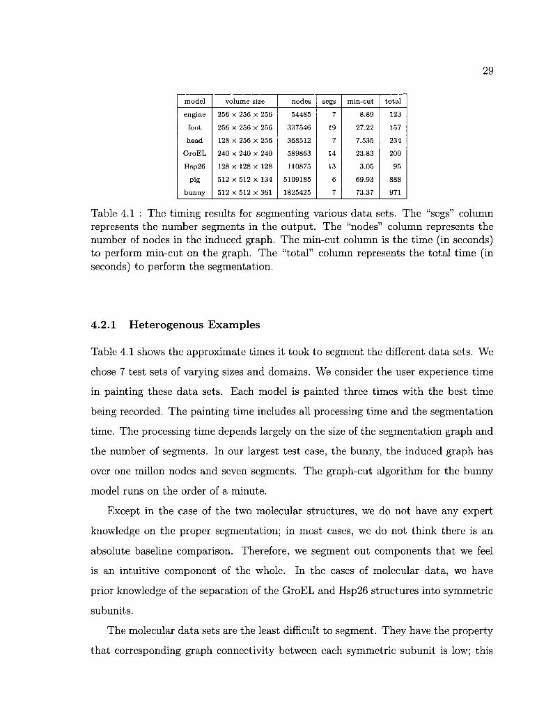
Table 4.1 : The timing results for segmenting various data sets. The "segs" column represents the number segments in the output. The "nodes" column represents the number of nodes in the induced graph. The min-cut column is the time (in seconds) to perform min-cut on the graph. The "total" column represents the total time (in seconds) to perform the segmentation.

4.2.1 Heterogenous Examples

Table 4.1 shows the approximate times it took to segment the different data sets. We

chose 7 test sets of varying sizes and domains. We consider the user experience time

in painting these data sets. Each model is painted three times with the best time

being recorded. The painting time includes all processing time and the segmentation

time. The processing time depends largely on the size of the segmentation graph and

the number of segments. In our largest test case, the bunny, the induced graph has

over one millon nodes and seven segments. The graph-cut algorithm for the bunny

model runs on the order of a minute.

Except in the case of the two molecular structures, we do not have any expert

knowledge on the proper segmentation; in most cases, we do not think there is an

absolute baseline comparison. Therefore, we segment out components that we feel

is an intuitive component of the whole. In the cases of molecular data, we have

prior knowledge of the separation of the GroEL and Hsp26 structures into symmetric

subunits.

The molecular data sets are the least difficult to segment. They have the property

that corresponding graph connectivity between each symmetric subunit is low; this

30

is exactly the optimal condition for the graph-cut to perform well. The two bone

data share this characteristics as the connectivity between bone fragments is low. As

indicated from Table 4.1, the time to segmenting each of the four data sets is less than

five minutes. The piggy bank and bunny data sets presented the most difficulty in our

tests. In all our tests, they were the largest in size. The time it took to perform single

min-cut segmentation was on the order of a minute, and this hindered interactivity

greatly. Furthermore, the piggy bank example was difficult due to the lack of distinct

separation between the coins the the inner surface of the pig. Also problematic was

the fact that the components were defined less by graph-connectivity and more by

curvature. Both of these factors componded to slow the segmentation. The bunny

example shared the connectivity/curvature problem, which contributed as well to its

slower times. However, the two data sets were segmented in around fifteen minutes

even with the aforementioned difficulties.

4.2.2 Protein Data Bank Examples

We have segmented datasets from the Protein Data Bank (PDB) entries. The PDB

models are specified as a set of atomic coordinates, where each atom can have se­

mantics attached to them. From the atomic coordinates, we build a volume over the

dataset by convolving the atoms with a radial function, such as a gaussian [17]. For

our purpose, we simply invoked the EMAN function pdb2mrc [16] to construct a vol­

ume over the input PDB. For comparison, we use a molecular visualization program

called UCSF Chimera [21]. Chimera colors protein entries by chains. By examin­

ing the models visually, we reproduced the chain segmentation using our painting

interface. Figure 4.1 illustrates that we were able to reproduce the segmentation

closely.

32

Chapter 5

Conclusion

We present a technique for multi-material classification in the context of segmenta­

tion of density maps. Our classification method provides a smoother boundary than

found in typical segmentation. Furthermore, it enables sub-voxel flexibility in shape-

representation. This alleviates artifacts and jaggedness that can occur in visualization

of segmented volumes.

We have also developed an intuitive segmentation interface that uses a graph-cut

approach to combine user-knowledge and simplicity in segmentation. We have shown

that our tool can be effectively used to rapidly create segmentation.

For our future work, we will experiment with using higher level interpolants such as

B-splines for classification. This will give us greater flexibility and accuracy in defining

the boundary between materials. Additionally, we will examine segmentation in the

context of large cryo-electron tomography, which current techniques cannot address

due to size and fidelity of the volume.

33

Bibliography

[1] BLOOMENTHAL, J. Implicit surfaces. Computer Aided Geometric Design 5

(1997), 341-355.

[2] CULLIP, T. J., AND NEUMANN, U. Accelerating volume reconstruction with

3d texture hardware. Tech. rep., Chapel Hill, NC, USA, 1994.

[3] DAHLHAUS, E., JOHNSON, D. S., PAPADIMITRIOU, C. H., SEYMOUR, P. D.,

AND YANNAKAKIS, M. The complexity of multiway cuts (extended abstract). In

STOC '92: Proceedings of the twenty-fourth annual ACM symposium on Theory

of computing (New York, NY, USA, 1992), ACM, pp. 241-251.

[4] ENGEL, K., KRAUS, M., AND ERTL, T. High-quality pre-integrated volume

rendering using hardware-accelerated pixel shading. In HWWS '01: Proceedings

of the ACM SIGGRAPH/EUROGRAPHICS workshop on Graphics hardware

(New York, NY, USA, 2001), ACM, pp. 9-16.

[5] FRISKEN, S. F. , PERRY, R. N., ROCKWOOD, A. P. , AND JONES, T. R.

Adaptively sampled distance fields: a general representation of shape for com­

puter graphics. In SIGGRAPH '00: Proceedings of the 27th annual conference

on Computer graphics and interactive techniques (New York, NY, USA, 2000),

ACM Press/Addison-Wesley Publishing Co., pp. 249-254.

[6] FUJIMORI, T., AND SUZUKI, H. Surface extraction from multi-material ct data.

In Computer Aided Design and Computer Graphics, 2005. Ninth International

Conference on (Dec. 2005), pp. 6 pp.-.

34

[7] GIBSON, S. F. F. Using distance maps for accurate surface representation in

sampled volumes. Volume Visualization and Graphics, IEEE Symposium on 0

(1998), 23-30.

[8] HADWIGER, M., BERGER, C , AND HAUSER, H. High-quality two-level volume

rendering of segmented data sets on consumer graphics hardware. In VIS '03:

Proceedings of the 14th IEEE Visualization 2003 (VIS'03) (Washington, DC,

USA, 2003), IEEE Computer Society, p. 40.

[9] Ju, T., LOSASSO, F. , SCHAEFER, S., AND WARREN, J. Dual contouring of

hermite data. In SIGGRAPH '02: Proceedings of the 29th annual conference

on Computer graphics and interactive techniques (New York, NY, USA, 2002),

ACM, pp. 339-346.

[10] KADOSH, A., COHEN-OR, D., AND YAGEL, R. Tricubic interpolation of dis­

crete surfaces for binary volumes. IEEE Transactions on Visualization and Com­

puter Graphics 9, 4 (2003), 580-586.

[11] KINDLMANN, G., AND DURKIN, J. W. Semi-automatic generation of transfer

functions for direct volume rendering. In VVS '98: Proceedings of the 1998

IEEE symposium on Volume visualization (New York, NY, USA, 1998), ACM,

pp. 79-86.

[12] KOBBELT, L. P. , BOTSCH, M., SCHWANECKE, U., AND SEIDEL, H.-P. Fea­

ture sensitive surface extraction from volume data. In SIGGRAPH '01: Pro­

ceedings of the 28th annual conference on Computer graphics and interactive

techniques (New York, NY, USA, 2001), ACM, pp. 57-66.

[13] LICHTENBELT, B., CRANE, R., AND NAQVI, S. Introduction to volume ren­

dering. Prentice-Hall, Inc., Upper Saddle River, NJ, USA, 1998.

[14] Liu, L., RABER, D., NOPACHAI, D., COMMEAN, P. , SINACORE, D., PRIOR,

F., PLESS, R., AND J U , T. Interactive separation of segmented bones in ct

35

volumes using graph cut. In MICCAI '08: Proceedings of the 11th international

conference on Medical Image Computing and Computer-Assisted Intervention -

Part I (Berlin, Heidelberg, 2008), Springer-Verlag, pp. 296-304.

[15] LORENSEN, W. E., AND CLINE, H. E. Marching cubes: A high resolution

3d surface construction algorithm. In SIGGRAPH '87: Proceedings of the 14th

annual conference on Computer graphics and interactive techniques (New York,

NY, USA, 1987), ACM, pp. 163-169.

[16] LUDTKE, S. J., BALDWIN, P . R., AND CHIU, W. Eman: Semiautomated

software for high-resolution single-particle reconstructions. Journal of Structural

Biology 128, 1 (1999), 82 - 97.

[17] MURAKI, S. Volumetric shape description of range data using "blobby model".

SIGGRAPH Comput. Graph. 25, 4 (1991), 227-235.

[18] OHTAKE, Y., BELYAEV, A., ALEXA, M., TURK, G., AND SEIDEL, H.-P.

Multi-level partition of unity implicits. In SIGGRAPH '05: ACM SIGGRAPH

2005 Courses (New York, NY, USA, 2005), ACM, p. 173.

[19] OWADA, S., NIELSEN, F., AND IGARASHI, T. Volume catcher. In I3D '05:

Proceedings of the 2005 symposium on Interactive 3D graphics and games (New

York, NY, USA, 2005), ACM, pp. 111-116.

[20] PAIVA, A., LOPES, H., LEWINER, T., AND DE FIGUEIREDO, L. Robust adap­

tive meshes for implicit surfaces. In Computer Graphics and Image Processing,

2006. SIBGRAPI '06. 19th Brazilian Symposium on (Oct. 2006), pp. 205-212.

[21] PETTERSEN, E. Ucsf chimera-a visualization system for exploratory research

and analysis. J. Comput. Chem. 25 (2004), 1605-1612.

[22] REZK-SALAMA, C , ENGEL, K., BAUER, M., GREINER, G., AND ERTL,

T. Interactive volume on standard pc graphics hardware using multi-textures

36

and multi-stage rasterization. In HWWS '00: Proceedings of the ACM SIG-

GRAPH/EUROGRAPHICS workshop on Graphics hardware (New York, NY,

USA, 2000), ACM, pp. 109-118.

[23] RlCCl, A. A Constructive Geometry for Computer Graphics. The Computer

Journal 16, 2 (may 1973), 157-160.

[24] SCHAEFER, S., AND WARREN, J. Dual contouring: "the secret sauce". Rice

University, Department of Computer Science Technical Report, 2003.

[25] SHAMMAA, M. H., SUZUKI, H., AND OHTAKE, Y. Extraction of isosurfaces

from multi-material ct volumetric data of mechanical parts. In SPM '08: Pro­

ceedings of the 2008 ACM symposium on Solid and physical modeling (New York,

NY, USA, 2008), ACM, pp. 213-220.

[26] STALLING, D., ZCKLER, M., AND HEGE, H. C. Interactive segmentation of

3d medical images with subvoxel accuracy. In Proc. CAR98 Computer Assisted

Radiology and Surgery (1998), pp. 137-142.

[27] T IEDE, U., SCHIEMANN, T., AND HOHNE, K. H. High quality rendering of at­

tributed volume data. In VIS '98: Proceedings of the conference on Visualization

'98 (Los Alamitos, CA, USA, 1998), IEEE Computer Society Press, pp. 255-262.

[28] WILSON, O., VANGELDER, A., AND WILHELMS, J. Direct volume rendering

via 3d textures. Tech. rep., Santa Cruz, CA, USA, 1994.

[29] YUAN, X., ZHANG, N., NGUYEN, M. X., AND CHEN, B. Volume cutout.

The Visual Computer (Special Issue of Pacific Graphics 2005) 21, 8-10 (2005),

745-754.