Propositional systems, Hilbert lattices

and generalized Hilbert spaces

Isar Stubbe∗ and Bart Van Steirteghem†

February 21, 2006‡

Abstract. With this chapter we provide a compact yet complete survey of two mostremarkable “representation theorems”: every arguesian projective geometry is repre-sented by an essentially unique vector space, and every arguesian Hilbert geometryis represented by an essentially unique generalized Hilbert space. C. Piron’s originalrepresentation theorem for propositional systems is then a corollary: it says that ev-ery irreducible, complete, atomistic, orthomodular lattice satisfying the covering lawand of rank at least 4 is isomorphic to the lattice of closed subspaces of an essen-tially unique generalized Hilbert space. Piron’s theorem combines abstract projectivegeometry with lattice theory. In fact, throughout this chapter we present the basiclattice theoretic aspects of abstract projective geometry: we prove the categoricalequivalence of projective geometries and projective lattices, and the triple categoricalequivalence of Hilbert geometries, Hilbert lattices and propositional systems.

Keywords: Projective geometry, projective lattice, Hilbert geometry, Hilbert lat-tice, propositional system, equivalence of categories, coproduct decomposition in irre-ducible components, Fundamental Theorems of projective geometry, RepresentationTheorem for propositional systems.

MSC 2000 Classification: 06Cxx (modular lattices, complemented lattices), 51A05(projective geometries), 51A50 (orthogonal spaces), 81P10 (quantum logic).

1. Introduction

Description of the problem. The definition of a Hilbert space H is all about a perfect marriagebetween linear algebra and topology: H is a vector space together with an inner product suchthat the norm associated to the inner product turns H into a complete metric space. As iswell-known for any vector space, the one-dimensional linear subspaces of H are the points of aprojective geometry, the collinearity relation being coplanarity. In other words, the set L(H) oflinear subspaces, ordered by inclusion, forms a so-called projective lattice.

∗Postdoctoral Fellow of the Research Foundation Flanders (FWO), Departement Wiskunde en Informatica,

Universiteit Antwerpen. E-mail: isar.stubbe@ua.ac.be†Partially supported by FCT/POCTI/FEDER, Departamento de Matematica, Instituto Superior Tecnico, Lis-

boa. E-mail: bvans@math.ist.utl.pt‡Final version published as: [I. Stubbe and B. Van Steirteghem, 2007] “Propositional systems, Hilbert lattices

and generalized Hilbert spaces”, Handbook of Quantum Logic and Quantum Structures: Quantum Structures (Eds.

K. Engesser, D. M. Gabbay and D. Lehmann), Elsevier, pp. 477–524.

1

GenHilb //

��

HilbGeom

��

oo ∼ // HilbLat oo ∼ //

��

PropSys

Vec // ProjGeom oo ∼ // ProjLat

Figure 1: A diagrammatic summary

Using the metric topology on H we can distinguish, amongst all linear subspaces, the closedones: we will note the set of these as C(H). In fact, the inner product on H induces an orthogo-nality operator on L(H) making it a Hilbert lattice, and the map

( )⊥⊥:L(H) //L(H):A 7→ A⊥⊥

is a closure operator on L(H) whose fixpoints are precisely the elements of C(H). For manyreasons, explained in detail elsewhere in this volume, it is the substructure C(H) ⊆ L(H) – andnot L(H) itself – which plays an important role in quantum logic; it is called a propositionalsystem.

In this survey paper we wish to explain the lattice theoretic axiomatization of such a prop-ositional system: we study necessary and sufficient conditions for an ordered set (C,≤) to beisomorphic to (C(H),⊆) for some (real, complex, quaternionic or generalized) Hilbert space H.As the above presentation suggests, this matter is intertwined with some deep results on projec-tive geometry.

Overview of contents. Section 2 of this paper presents the relevant definitions of, and somebasic results on, abstract (also called ‘modern’ or ‘synthetic’) projective geometry. Following Cl.-A. Faure and A. Frolicher’s [2000] reference on the subject, we define a ‘projective geometry’ as aset together with a ternary collinearity relation (satisfying suitable axioms). The one-dimensionalsubspaces of a vector space are an example of such a projective geometry, with coplanarity as theternary relation. After discovering some particular properties of the ordered set of ‘subspaces’ ofsuch a projective geometry, we make an abstraction of this ordered set and call it a ‘projectivelattice’. We then speak of ‘morphisms’ between projective geometries, resp. projective lattices,and show that the category ProjGeom of projective geometries and the category ProjLat of projec-tive lattices are equivalent. Vector spaces and ‘semilinear maps’ form a third important categoryVec, and there is a functor Vec // ProjGeom. The bottom row in figure 1 summarizes this.

A projective geometry for which every line contains at least three points, is said to be ‘irre-ducible’. We deal with these in section 3, for this geometric fact has an important categorical sig-nificance [Faure and Frolicher, 2000]: a projective geometry is irreducible precisely when it is nota non-trivial coproduct in ProjGeom, and every projective geometry is the coproduct of irreducibleones. By the categorical equivalence between ProjGeom and ProjLat, the “same” result holds forprojective lattices. The projective geometries in the image of the functor Vec // ProjGeom arealways irreducible.

Having set the scene, we deal in section 4 with the linear representation of projective geome-tries (of dimension at least 2) and their morphisms, i.e. those objects and morphisms that lie inthe image of the functor Vec // ProjGeom. The First Fundamental Theorem, which is by nowpart of mathematical folklore, says that precisely the ‘arguesian’ geometries (which include allgeometries of dimension at least 3) are “linearizable”. The Second Fundamental Theorem charac-

2

terizes the “linearizable” morphisms. [Holland, 1995, §3] and [Faure, 2002] have some commentson the history of these results. We outline the proof of the First Fundamental Theorem as givenin [Beutelspacher and Rosenbaum, 1998]; for a short proof of the Second Fundamental Theoremwe refer to [Faure, 2002].

Again following [Faure and Frolicher, 2000], we turn in section 5 to projective geometriesthat come with a binary orthogonality relation which satisfies certain axioms: so-called ‘Hilbertgeometries’. The key example is given by the projective geometry of one-dimensional subspacesof a ‘generalized Hilbert space’ (a notion due to C. Piron [1976]), with the orthogonality inducedby the inner product. The projective lattice of subspaces of such a Hilbert geometry inherits anorthogonality operator which satisfies some specific conditions, and this leads to the notion of‘Hilbert lattice’. The elements of a Hilbert lattice that equal their biorthogonal are said to be‘(biorthogonally) closed’; they form a ‘propositional system’ [Piron, 1976]: a complete, atomistic,orthomodular lattice satisfying the covering law. Considering Hilbert geometries, Hilbert latticesand propositional systems together with suitable (‘continuous’) morphisms, we obtain a tripleequivalence of the categories HilbGeom, HilbLat and PropSys. And there is a category GenHilb ofgeneralized Hilbert spaces and continuous semilinear maps, with a functor GenHilb // HilbGeom.Since a Hilbert geometry is a projective geometry with extra structure, and a continuous morph-ism between Hilbert geometries is a particular morphism between (underlying) projective ge-ometries, there is a faithful functor HilbGeom // ProjGeom. Similarly there are faithful functorsHilbLat // ProjLat and GenHilb // Vec too, and the resulting (commutative) diagram of categoriesand functors is sketched in figure 1.

Then we show in section 6 that a Hilbert geometry is irreducible (as a projective geometry, i.e.each line contains at least three points) if and only if it is not a non-trivial coproduct in HilbGeom;and each Hilbert geometry is the coproduct of irreducible ones. By categorical equivalence, the“same” is true for Hilbert lattices and propositional systems.

In section 7 we present the Representation Theorem for propositional systems or, equivalently,Hilbert geometries (of dimension at least 2): the arguesian Hilbert geometries constitute the imageof the functor GenHilb // HilbGeom. For finite dimensional geometries this result is due to G.Birkhoff and J. von Neumann [1936] while the more general (infinite-dimensional) version goesback to C. Piron’s [1964, 1976] representation theorem: every irreducible propositional system ofrank at least 4 is isomorphic to the lattice of closed subspaces of an essentially unique generalizedHilbert space. We provide an outline of the proof given in [Holland, 1995, §3].

The final section 8 contains some comments and remarks on various interesting points thatwe did not address or develop in the text.

Required lattice and category theory. Throughout this chapter we use quite a few notionsand (mostly straightforward) facts from lattice theory. For completeness’ sake we have addeda short appendix in which we explain the words marked with a “†” in our text. The standardreferences on lattice theory are [Birkhoff, 1967; Gratzer, 1998], but [Maeda and Maeda, 1970;Kalmbach, 1983] have everything we need too. Finally, we also use some very basic categorytheory: we speak of an ‘equivalence of categories’, compute some ‘coproducts’, and talk about‘full’ and ‘faithful’ functors. Other categorical notions that we need, are explained in the text.The classic [Mac Lane, 1971] or the first volume of [Borceux, 1994] contain all this (and muchmore).

Acknowledgements. As students of the ’98 generation in mathematics in Brussels, both authorsprepared a diploma dissertation on topics related to operational quantum logic, supervised and

3

��

��

��

��

�

���������

• •

•

•

•

•

a c q

b

p

d

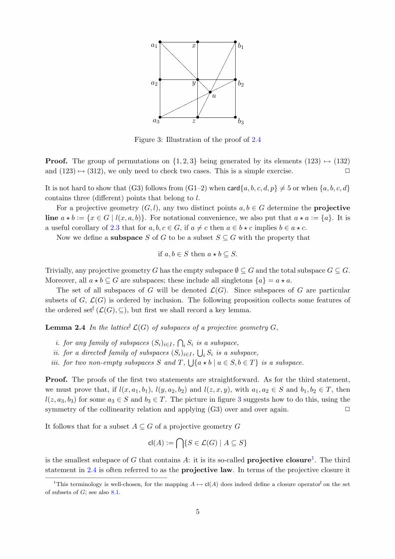
Figure 2: Illustration of (G3)

surrounded by some of the field’s most outstanding researchers—Dirk Aerts, Bob Coecke, FrankValckenborgh. Moreover, the quantum physics group in Brussels being next of kin to ConstantinPiron’s group in Geneva, we also had the chance to interact with the members of the latter—Claude-Alain Faure, Constantin Piron, David Moore. It is with great pleasure that we dedicatethis chapter to all those who made that period unforgettable. We thank Mathieu Dupont, Claude-Alain Faure, Chris Heunen and Frank Valckenborgh for their comments and suggestions.

2. Projective geometries, projective lattices

It is a well-known slogan in mathematics that “the lines of a vector space are the points of aprojective geometry”. To make this statement precise, we must introduce the abstract notion ofa ‘projective geometry’.

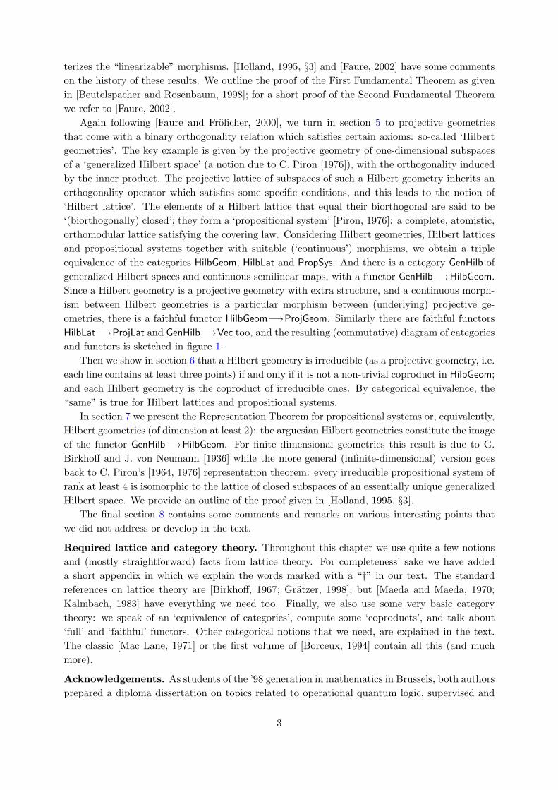
Definition 2.1 A projective geometry (G, l) is a set G of points together with a ternarycollinearity relation l ⊆ G×G×G such that

(G1) for all a, b ∈ G, l(a, b, a),(G2) for all a, b, p, q ∈ G, if l(a, p, q), l(b, p, q) and p 6= q, then l(a, b, p),(G3) for all a, b, c, d, p ∈ G, if l(p, a, b) and l(p, c, d) then there exists a q ∈ G such that l(q, a, c)

and l(q, b, d).

Often, since no confusion will arise, we shall speak of “a projective geometryG”, without explicitlymentioning its collinearity relation l. The axioms for the collinearity relation – as well as manyof the calculations further on – are best understood by means of a simple picture, in which onedraws “dots” for the points of G, and a “line” through any three points a, b, c such that l(a, b, c).With this intuition (which will be made exact further on), (G1) and (G2) say that two distinctpoints determine one and only one line, and (G3) is depicted in figure 2.

Example 2.2 Let V be a (left) vector space over a (not necessarily commutative) field K. Theset of lines of V endowed with the coplanarity relation forms a projective geometry; it will bedenoted further on as P(V ). Note that the collinearity relation is trivial when dim(V ) ≤ 2.

The example P(V ) is very helpful for sharpening the intuition on abstract projective geometry.For example, it is clear that the collinearity relation in P(V ) is symmetric; but in fact thisproperty holds also in the general case.

Lemma 2.3 A ternary relation l on a set G satisfying (G1–2) is symmetric, meaning that fora1, a2, a3 ∈ G, if l(a1, a2, a3) then also l(aσ(1), aσ(2), aσ(3)) for any permutation σ on {1, 2, 3}.

4

������������

������������

@@

@@

@@

@@

a1

a2

a3

x

y

z

b1

b2

b3

u

•

•

•

• •

•

•

•

•

•

•

Figure 3: Illustration of the proof of 2.4

Proof. The group of permutations on {1, 2, 3} being generated by its elements (123) 7→ (132)and (123) 7→ (312), we only need to check two cases. This is a simple exercise. 2

It is not hard to show that (G3) follows from (G1–2) when card{a, b, c, d, p} 6= 5 or when {a, b, c, d}contains three (different) points that belong to l.

For a projective geometry (G, l), any two distinct points a, b ∈ G determine the projectiveline a ? b := {x ∈ G | l(x, a, b)}. For notational convenience, we also put that a ? a := {a}. It isa useful corollary of 2.3 that for a, b, c ∈ G, if a 6= c then a ∈ b ? c implies b ∈ a ? c.

Now we define a subspace S of G to be a subset S ⊆ G with the property that

if a, b ∈ S then a ? b ⊆ S.

Trivially, any projective geometry G has the empty subspace ∅ ⊆ G and the total subspace G ⊆ G.Moreover, all a ? b ⊆ G are subspaces; these include all singletons {a} = a ? a.

The set of all subspaces of G will be denoted L(G). Since subspaces of G are particularsubsets of G, L(G) is ordered by inclusion. The following proposition collects some features ofthe ordered set† (L(G),⊆), but first we shall record a key lemma.

Lemma 2.4 In the lattice† L(G) of subspaces of a projective geometry G,

i. for any family of subspaces (Si)i∈I ,⋂

i Si is a subspace,ii. for a directed† family of subspaces (Si)i∈I ,

⋃i Si is a subspace,

iii. for two non-empty subspaces S and T ,⋃{a ? b | a ∈ S, b ∈ T} is a subspace.

Proof. The proofs of the first two statements are straightforward. As for the third statement,we must prove that, if l(x, a1, b1), l(y, a2, b2) and l(z, x, y), with a1, a2 ∈ S and b1, b2 ∈ T , thenl(z, a3, b3) for some a3 ∈ S and b3 ∈ T . The picture in figure 3 suggests how to do this, using thesymmetry of the collinearity relation and applying (G3) over and over again. 2

It follows that for a subset A ⊆ G of a projective geometry G

cl(A) :=⋂{S ∈ L(G) | A ⊆ S}

is the smallest subspace of G that contains A: it is its so-called projective closure1. The thirdstatement in 2.4 is often referred to as the projective law. In terms of the projective closure it

1This terminology is well-chosen, for the mapping A 7→ cl(A) does indeed define a closure operator† on the set

of subsets of G; see also 8.1.

5

may be stated as: for non-empty subspaces S and T of G,

cl(S ∪ T ) =⋃{a ? b | a ∈ S, b ∈ T}.

Proposition 2.5 For any projective geometry G, (L(G),⊆) is a complete†, atomistic†, continuous†

, modular† lattice.

Proof. The order on L(G) is complete, because the intersection of subspaces is their infimum†;thus the supremum† of a family (Si)i∈I ∈ L(G) is

∨i Si = cl(

⋃i Si). This makes it at once clear

that any subspace S ∈ L(G) is the supremum of its points: S = cl(S) =∨

a∈S{a}; and singletonsubspaces being exactly the atoms†of L(G) this also shows that L(G) is atomistic. The continuityof L(G) follows trivially from the fact that directed suprema in L(G) are simply unions. Finally,to show that L(G) is modular, it suffices to verify that for non-empty subspaces S, T, U ⊆ G, ifS ⊆ T then (S ∨U)∩ T ⊆ S ∨ (U ∩ T ). We are going to use the projective law a couple of times.Suppose that x ∈ (S ∨ U) ∩ T ; so x ∈ T , but also x ∈ S ∨ U , which means that x ∈ a ? b forsome a ∈ S and b ∈ U . If x = a then x ∈ S ⊆ S ∨ (U ∩ T ); if x 6= a then x ∈ a ? b implies thatb ∈ a ? x ⊆ S ∨ T = T (using that S ⊆ T ) so that x ∈ a ? b ⊆ S ∨ (U ∩ T ) in this case too. 2

Definition 2.6 An ordered set (L,≤) is a projective lattice if it is a complete, atomistic,continuous, modular lattice.

There are equivalent formulations for the definition of ‘projective lattice’; we shall encounter somefurther on in this section. Here we shall already give one alternative for the continuity condition,which is sometimes easier to handle and will be used in the proofs of 2.16 and 3.8.

Lemma 2.7 A complete atomistic lattice L is continuous if and only if its atoms are compact,i.e. if a is an atom and (xi)i∈I is a directed family in L, then a ≤

∨i xi implies a ≤ xk for some

k ∈ I.

Proof. If L is continuous and (with notations as in the statement of the lemma) a ≤∨

i xi, thena = a ∧ (

∨i xi) =

∨i(a ∧ xi), so there must be a k ∈ I for which a ∧ xk 6= 0, whence a ≤ xk (for

a is an atom). Conversely,∨

i(y ∧ xi) ≤ y ∧ (∨

i xi) holds for any element y ∈ L. Suppose thatthis inequality is strict. By atomisticity of L there must exist an atom a such that a 6≤

∨i(y∧xi)

and a ≤ y ∧ (∨

i xi). This implies in particular that a ≤ y and a ≤∨

i xi, and by hypothesis ais compact so that a ≤ xk for some k ∈ I. But then a ≤ y ∧ xk ≤

∨i(y ∧ xi) is a contradiction.

Thus necessarily∨

i(y ∧ xi) = y ∧ (∨

i xi) for every y ∈ L. 2

Example 2.8 For a K-vector space V , the set L(V ) of linear subspaces, ordered by set-inclusion,is isomorphic to the projective lattice L(P(V )) of subspaces of the projective geometry P(V ) of2.2: the mappings

L(V ) //L(P(V )):W 7→ P(W )

L(P(V )) //L(V ):S 7→ {x ∈ V | Kx ∈ S} ∪ {0}

are well-defined, preserve order† and are each other’s inverse. With slight abuse of notation weshall write L(V ) even when we actually mean L(P(V )).

6

So 2.5 states that a projective geometry G determines a projective lattice L(G); but theconverse is also true. First we prove a lattice theoretical lemma that exhibits the strength of themodularity condition.

Lemma 2.9 Let L be a complete atomistic lattice, and G(L) its set of atoms.

i. If L is modular, then it is both upper semimodular† and lower semimodular†.ii. L is upper semimodular if and only if it satisfies the covering law†.iii. If L is lower semimodular and satisfies the covering law then it has the intersection prop-

erty: for any x ∈ L and p, q ∈ G(L) with p 6= q, if p ≤ q ∨ x then (p ∨ q) ∧ x 6= 0.iv. If L has the intersection property, then for a, b, c ∈ G(L) with a 6= b, if a ≤ b ∨ c then also

c ≤ a ∨ b.v. If L has the intersection property, then G(L) forms a projective geometry for the ternary

relationl(a, b, c) if and only if a ≤ b ∨ c or b = c. (1)

Proof. (i) For any lattice L, the maps

ϕ: [u ∧ v, v] // [u, u ∨ v]:x 7→ x ∨ u and ψ: [u, u ∨ v] // [u ∧ v, v]: y 7→ y ∧ v

are well-defined and preserve order. If L is modular then moreover ψ(ϕ(x)) = (x ∨ u) ∧ v =x∨ (u∧ x) = x; similarly ϕ(ψ(y)) = y. So the two segments are isomorphic lattices. Now clearlyu ∧ v l v ⇔ card[u ∧ v, v] = 2 ⇔ card[u, u ∨ v] = 2 ⇔ u l u ∨ v, which proves both upper andlower semimodularity of L (resp. ⇒ and ⇐ in this equivalence).

(ii) The covering law is a special case of upper semimodularity. Conversely, in an atomisticlattice satisfying the covering law it is the case that

xl y if and only if there exists a ∈ G(L) : a 6≤ x, x ∨ a = y. (2)

(Indeed, the “only if” follows from atomisticity, and the “if” is the covering law.) So if nowu ∧ v l v then there is an atom a ∈ G(L) such that a 6≤ u ∧ v and (u ∧ v) ∨ a = v. But thenu ∨ v = u ∨ [(u ∧ v) ∨ a)] = [u ∨ (u ∧ v)] ∨ a = u ∨ a; and a 6≤ u (for a ≤ v but a 6≤ u ∧ v) so by(2) we conclude that ul u ∨ v.

(iii) Let p 6= q ∈ G(L) and x ∈ L be such that p ≤ q∨x. If q ≤ x then trivially q ≤ (p∨ q)∧x;if q 6≤ x then x l q ∨ x = (p ∨ q) ∨ x by the covering law and the hypothesis p ≤ q ∨ x. This inturn implies x∧ (p∨ q) l p∨ q by lower semimodularity. Now x∧ (p∨ q) 6= 0 because it is coveredby p ∨ q which is not an atom.

(iv) From the assumptions and the intersection property it follows that (a∨ b)∧ c 6= 0, so thatnecessarily c ≤ a ∨ b, for c is an atom.

(v) We shall check the axioms in 2.1, using the notations introduced there and keeping in mindthat the collinearity relation is as in (1). Axiom (G1) is trivial. For (G2) we may suppose thatb 6= p. Then, by (iv), b ≤ p∨q implies q ≤ b∨p and hence a ≤ p∨q ≤ p∨(b∨p) = p∨b, as wanted.As for (G3), we may suppose that a, b, c, d, and p are different points; then p ≤ a ∨ b impliesa ≤ p ∨ b, hence a ≤ b ∨ c ∨ d, and therefore, by the intersection property, (b ∨ d) ∧ (a ∨ c) 6= 0,which means (by atomisticity) that q ≤ (b ∨ d) ∧ (a ∨ c) for some q ∈ G(L), as wanted. 2

The lemma above is not stated as “sharply” as possible. In fact, the ‘intersection property’ in(iii) can be rephrased for an arbitrary lattice L with 0 as

if p ≤ q ∨ x then there exists an atom r such that r ≤ (p ∨ q) ∧ x

7

for atoms p 6= q and an arbitrary x; this is how it first appeared in [Faure and Frolicher, 1995].Then statement (i), sufficiency in (ii), and statement (iii) are true for any lattice with 0 (notnecessarily complete nor atomistic), while the converse of (iii) holds for an atomistic L. We shallonly need these results for a complete atomistic lattice L (in 2.10 below and also in 5.11 furtheron).

We may now state the following as a simple corollary of 2.9.

Proposition 2.10 The set G(L) of atoms of a projective lattice L forms a projective geometryfor the ternary relation in (1).

If L is a lattice with 0 for which G(L) is a projective geometry for the collinearity in (1),then L(G(L)) is a projective lattice, according to 2.5. Would L be isomorphic to L(G(L)) thennecessarily L must be a projective lattice too: completeness, atomisticity, continuity and mod-ularity are transported by isomorphism. From the work in the rest of this section it will followthat L being projective is also sufficient for it to be naturally isomorphic to L(G(L)). Similarlyit is also true that a projective geometry G may be identified with G(L(G)). More precisely, weshall show that projective geometries and projective lattices are categorically equivalent notions.So we better start building categories!

Recall first that a partial map f between sets A and B is a map from a subset Df ⊆ A toB. The set Df is the domain of f , and the set-complement Kf = (Df )c is its kernel. Most ofthe time we write such a partial map as f :A //__ B instead of f :A \Kf

//B or f :Df ⊆ A //B.Partial maps compose: for f :A //__ B with kernel Kf and g:B //__ C with kernel Kg, g ◦f :A //__ C

has kernel Kf ∪ f−1(Kg) and maps an element a of its domain to g(f(a)). This compositionlaw is associative, and the identity map on a set (viewed as partial map with empty kernel) is atwo-sided identity for this composition. That is to say, there is a perfectly good category ParSet

of sets and partial maps.

Definition 2.11 Given two projective geometries G1 and G2, a partial map g:G1//__ G2 is a

morphism of projective geometries if, for any subspace T of G2,

g∗(T ) := Kg ∪ g−1(T )

is a subspace of G1.

Since ∅ ⊆ G2 is a subspace, the kernel Kg of g:G1//__ G2 must be a subspace of G1. In the proof

of 3.7 we shall show that a morphism g:G1//__ G2 maps any line a?b in G1, with a, b 6∈ Kg, either

to a single point of G2 (in case g(a) = g(b)) or injectively to the line g(a) ? g(b) of G2 (in caseg(a) 6= g(b)). This provides a geometric interpretation, in terms of points and lines, of the notionof ‘morphism between projective geometries’. (As a matter of fact, these latter conditions arealso sufficient for g to be a morphism, provided that Kg = ∅.)

With composition of two morphisms of projective geometries defined as the composition ofthe underlying partial maps, we obtain a category ProjGeom. An isomorphism in ProjGeom is, asin any category, a morphism g:G1

//__ G2 with a two-sided inverse g′:G2//__ G1. But it can easily

be seen that such is the same as a bijection (with empty kernel) g:G1//G2 which preserves and

reflects the collinearity relation: l1(a, b, c) if and only if l2(g(a), g(b), g(c)) for all a, b, c ∈ G1.

Example 2.12 By definition, a semilinear map between a K1-vector space V1 and a K2-vector space V2 is an additive map f :V1

// V2 for which there exists a homomorphism of fields

8

σ:K1//K2 such that f(αx) = σ(α)f(x) for every α ∈ K1 and x ∈ V1. Sometimes we call this a

σ-linear map f :V1// V2 too. The σ is uniquely determined by f whenever f is non-zero; and

the zero-map is semilinear if and only if there exists a homomorphism σ:K1//K2. There is a

category Vec of vector spaces and semilinear maps. A semilinear map f :V1// V2 determines a

morphism of projective geometries

P(f):P(V1) //__ P(V2):K1x 7→ K2f(x) with kernel P(ker(f)).

This, in fact, defines a functor

P:Vec // ProjGeom:(f :V1

// V2

)7→

(P(f):P(V1) //__ P(V2)

).

The following example [Faure and Frolicher, 2000, 6.3.9–11] shows that semilinear maps canbehave surprisingly when the associated field homomorphism is not an isomorphism.

Example 2.13 Let F be a commutative field, let K := F (x) be the field of rational functions andlet n be a positive integer. Consider the field homomorphism σ:K //K: q(x) 7→ q(xn). One canshow that σ(K) ⊆ K is an extension of fields of degree n: putting αi := xi−1, the set {α1, . . . , αn}forms a basis of K over σ(K). It follows that ϕ:Kn //K: (a1, . . . , an) 7→ σ(a1)α1 + . . .+σ(an)αn

is a σ-linear form with zero kernel. Moreover, picking any nonzero b ∈ Kn we obtain a σ-linearmap f :Kn //Kn:x 7→ ϕ(x)b for which P(f) is constant and which has empty kernel.

We now turn to projective lattices.

Definition 2.14 Given projective lattices L1 and L2, a map f :L1//L2 is a morphism of

projective lattices if it preserves arbitrary suprema and sends atoms in L1 to atoms or to thebottom element in L2.

We thus get a category ProjLat. Note that an isomorphism in ProjLat is indeed the same thing asan order-preserving and reflecting bijection, so that in 2.8 there is no doubt about the meaningof the word.

We know from 2.5 that any projective geometry G determines a projective lattice L(G); andany projective lattice L determines a projective geometry G(L) according to 2.10. For morphismswe can play a similar game.

Proposition 2.15 If g:G1//__ G2 is a morphism of projective geometries, then

L(g):L(G1) //L(G2):S 7→⋂{T ∈ L(G2) | S ⊆ g∗(T )}

is a morphism of projective lattices. And if f :L1//L2 is a morphism of projective lattices, then

G(f):G(L1) //__ G(L2): a 7→ f(a) with kernel {a ∈ G(L1) | f(a) = 0}

is a morphism of projective geometries.

Proof. First note that g:G1//__ G2 defines the “inverse image” map

g∗:L(G2) //L(G1):T 7→ Kg ∪ g−1(T ),

which preserves arbitrary intersections. Intersections of subspaces being their infima, g∗ musthave a left adjoint†. This left adjoint is precisely L(g), which proves that L(g) preserves arbitrary

9

suprema. The atoms of L(G1) and L(G2) corresponding to their respective singleton subspaces,L(g) sends atoms to atoms or to the bottom element.

Because f :L1//L2 sends atoms of L1 to atoms or the bottom element of L2, G(f) is a

well-defined partial map. Now let T ⊆ G(L2) be a subspace of the projective geometry G(L2); ifa, b ∈ G(f)∗(T ) and c ≤ a∨ b then f(c) ≤ f(a∨ b) = f(a)∨ f(b), showing that either f(c) = 0 orf(c) ∈ T (by T being a subspace). That is to say, G(f)∗(T ) is a subspace of G1. 2

The above proposition explains the requirement in 2.14 that a morphism of projective latticespreserve arbitrary suprema: such a morphism must be thought of as the left adjoint to an inverseimage.

Now we are ready to state and prove the result promised a while ago.

Theorem 2.16 The categories ProjGeom and ProjLat are equivalent. To wit, the assignments

L:ProjGeom // ProjLat:(g:G1

//__ G2

)7→

(L(g):L(G1) //L(G2)

)G:ProjLat // ProjGeom:

(f :L1

//L2

)7→

(G(f):G(L1) //__ G(L2)

)are functorial, and for a projective geometry G and a projective lattice L there are natural iso-morphisms

αG:G ∼ // G(L(G)): a 7→ {a},βL:L ∼ //L(G(L)):x 7→ {a ∈ G(L) | a ≤ x}.

Proof. It is a matter of straightforward calculations to see that L and G are functorial. Weshall prove that αG and βL are isomorphisms, and leave the verification of their naturality to thereader.

First, the map αG is obviously a well-defined bijection (with empty kernel): the atoms ofL(G) are precisely the singleton subsets of G, i.e. the points of G. We need to show that a, b, care collinear in G if and only if {a}, {b}, {c} are collinear in G(L(G)); but this comes down toshowing that a ∈ b ? c in G if and only if {a} ⊆ {b} ∨ {c} in L(G), which is an instance of theprojective law.

Next, it is easy to see that βL is a well-defined map, i.e. that any βL(x) ⊆ G(L) is indeed asubspace (for the collinearity relation on G(L) as in 2.10). We claim now that the map

γL:L(G(L)) 7→ L:S 7→∨S

is the inverse of βL in ProjLat. In fact, it is clear that both βL and γL preserve order; thus it sufficesto show that they are mutually inverse maps to prove that they constitute an isomorphism inProjLat. That γL◦βL is the identity, is the atomisticity of L. Conversely, for a subspace S ⊆ G(L)we have that (βL ◦ γL)(S) = {a ∈ G(L) | a ≤

∨S}; so it suffices to prove that a ≤

∨S ⇔ a ∈ S

to find that βL ◦ γL is the identity on L(G(L)). But∨S =

∨{∨S′ | S′ ⊆f S} – where we

write S′ ⊆f S for a finite subset – which expresses∨S as a directed join of finite joins. Because

the atoms of L are compact (by continuity and 2.7), a ≤∨S if and only if a ≤

∨S′ for some

S′ ⊆f S. Using the intersection property of L (cf. 2.9 and 2.10) and using the subspace propertyof S for the collinearity relation on G(L), we shall prove by induction on the number of elementsof S′ = {s1, ..., sn} that a ∈ S. The case n = 1 is trivial, so let the case n−1 be true by inductionhypothesis, and let a ≤ s1∨ ...∨ sn−1∨ sn with sn 6≤ s1∨ ...∨ sn−1. If a ≤ sn then a = sn ∈ S and

10

"!#

TT

TT

TT�

��

��

�""

""

"

bb

bb

b •

•

•• •

••

Figure 4: The smallest non-trivial irreducible geometry

we are done. If a 6≤ sn then a 6= sn and by the intersection property (s1∨ ...∨sn−1)∧ (sn∨a) 6= 0,so (by atomisticity) there is an atom r ∈ G(L) such that r ≤ (s1 ∨ ... ∨ sn−1) ∧ (sn ∨ a). Butthen r ≤ s1 ∨ ... ∨ sn−1 thus r ∈ S by the induction hypothesis. And since r 6= sn (for otherwisesn ≤ s1 ∨ ... ∨ sn−1), r ≤ sn ∨ a implies a ≤ r ∨ sn by (iv) of 2.9, so that a ∈ S by S being asubspace. 2

In the proof for βL:L //L(G(L)) being an isomorphism, modularity of L was not explicitly used,except for the fact that it implies the intersection property as in 2.9. Therefore, since L ∼= L(G(L))and the latter is a projective lattice, it follows that a complete, atomistic, continuous lattice ismodular if and only if it has the intersection property.

Until now we have considered the following diagram of categories and functors:

Vec // ProjGeom oo ∼ // ProjLat.

In section 4 we shall discuss a converse to the functor P:Vec // ProjGeom, but thereto we needto deal with another issue first.

3. Irreducible components

However trivial it may seem that every plane in a vector space V contains at least three lines,this is actually not automatic for abstract projective geometries.

Definition 3.1 A projective geometry (G, l) is irreducible if for every a, b ∈ G, card(a ? b) 6= 2;otherwise it is reducible.

Since we defined that a?a = {a}, this definition says that G is an irreducible projective geometryprecisely when every line contains at least three points. This definition is clearly invariant underisomorphism.

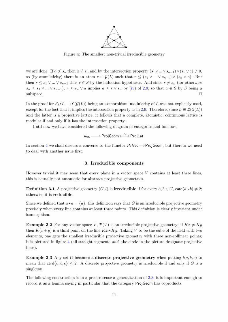
Example 3.2 For any vector space V , P(V ) is an irreducible projective geometry: if Kx 6= Ky

then K(x+y) is a third point on the line Kx?Ky. Taking V to be the cube of the field with twoelements, one gets the smallest irreducible projective geometry with three non-collinear points;it is pictured in figure 4 (all straight segments and the circle in the picture designate projectivelines).

Example 3.3 Any set G becomes a discrete projective geometry when putting l(a, b, c) tomean that card{a, b, c} ≤ 2. A discrete projective geometry is irreducible if and only if G is asingleton.

The following construction is in a precise sense a generalization of 3.3; it is important enough torecord it as a lemma saying in particular that the category ProjGeom has coproducts.

11

Lemma 3.4 Given a family (Gi, li)i∈I of projective geometries, the disjoint union⊎

iGi equippedwith the relation

l(a, b, c) if either card{a, b, c} ≤ 2 or lk(a, b, c) in Gk for some k ∈ I,

together with the inclusionssk:Gk

//⊎i

Gi: a 7→ a (3)

is a coproduct in ProjGeom.

Proof. First we check that⊎

iGi forms a projective geometry for the indicated collinearityrelation; we shall verify axioms (G1–3) in 2.1, keeping the notations used there. For (G1) there isnothing to prove. Axiom (G2) is trivial when we have card{a, b, p} 6= 3; from now on we assumethe contrary. If a = q then l(b, p, q) means that b, p, a ∈ Gk and lk(b, p, a) for some k ∈ I becauseof the previous assumption, but then lk(a, b, p) by symmetry of lk and hence l(a, b, p) as wanted;so suppose a 6= q. The hypothesis l(a, p, q) now implies that a, p, q ∈ Gk and lk(a, p, q) for somek ∈ I; but then also b ∈ Gk and lk(b, p, q) by l(b, p, q); so (G2) for (

⊎iGi, l) follows from (G2)

for (Gk, lk). Finally, it suffices to check (G3) in the case where card{a, b, c, d, p} = 5; but bythe hypotheses l(p, a, b) and l(p, c, d) these points must then all lie in the same Gk and satisfylk(p, a, b) and lk(p, c, d); so applying (G3) to (Gk, lk) proves (G3) for (

⊎iGi, l).

From the definition of the projective geometry (⊎

iGi, l) it follows directly that, for a, b ∈⊎iGi, a ? b = a ?k b if a, b ∈ Gk and a ? b = {a, b} otherwise. From this it follows in turn that a

subset S ⊆⊎

iGi is a subspace if and only if, for every k ∈ I, S ∩ Gk is a subspace of Gk. Butthen, referring to the maps in (3), since s∗k(S) = S ∩Gk these maps are morphisms (with emptykernels) of projective geometries, forming a cocone in ProjGeom.

Suppose finally that (gk:Gk//__ G)k∈I is another cocone in ProjGeom; we claim that

g:⊎i

Gi//__ G: a 7→ gk(a) if a ∈ Gk \Kgk

, with kernel⊎i

Kgi

is the unique morphism of projective geometries satisfying g ◦ sk = gk for all k ∈ I. To see this,note first that g∗(S) =

⊎i g

∗i (S) for a subspace S ⊆ G; so g∗(S)∩Gk = g∗k(S) for k ∈ I, and since

these are subspaces of the respective Gk’s, it follows that g∗(S) is a subspace of⊎

iGi. Hence gis a morphism of projective geometries; and obviously g ◦ sk = gk for all k ∈ I. If g:

⊎iGi

//__ G

is another such morphism, then necessarily Kg = g∗(∅) =⊎

iKgi = Kg; and for a ∈ Gk \ Kgk,

g(a) = g(sk(a)) = gk(a) = g(sk(a)) = g(a). That is to say, g = g, and we thus verified theuniversal property of the cocone in (3). 2

Clearly, any coproduct of two or more (non-empty) projective geometries is reducible. In fact, adiscrete projective geometry G as in 3.3 is nothing but the coproduct of the singleton projectivegeometries ({a})a∈G.

As the terminology suggests, every projective geometry G can be “reduced” to a coproduct ofirreducible ones. Note first that a subspace S ⊆ G of a projective geometry (G, l) is a projectivegeometry for the inherited collinearity relation; and the inclusion S ↪→ G is then a morphism (withempty kernel) of projective geometries. We say that S ⊆ G is an irreducible subspace when it isirreducible as projective geometry in its own right; and S is a maximal irreducible subspaceif moreover it is not strictly contained in any other irreducible subspace. This terminology isconsistent: a projective geometry G is irreducible if and only if G ⊆ G is a (trivially maximal)irreducible subspace.

12

��

��

��

��

�

•

•• ••

•

ac

zx

b

y

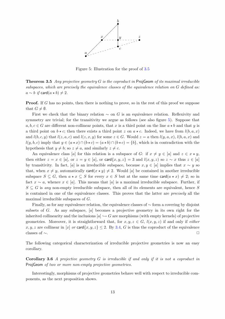
Figure 5: Illustration for the proof of 3.5

Theorem 3.5 Any projective geometry G is the coproduct in ProjGeom of its maximal irreduciblesubspaces, which are precisely the equivalence classes of the equivalence relation on G defined as:a ∼ b if card(a ? b) 6= 2.

Proof. If G has no points, then there is nothing to prove, so in the rest of this proof we supposethat G 6= ∅.

First we check that the binary relation ∼ on G is an equivalence relation. Reflexivity andsymmetry are trivial; for the transitivity we argue as follows (see also figure 5). Suppose thata, b, c ∈ G are different non-collinear points, that x is a third point on the line a ? b and that y isa third point on b ? c; then there exists a third point z on a ? c. Indeed, we have from l(b, a, x)and l(b, c, y) that l(z, a, c) and l(z, x, y) for some z ∈ G. Would z = a then l(y, a, x), l(b, a, x) andl(y, b, c) imply that y ∈ (a ? x)∩ (b ? c) = (a ? b)∩ (b ? c) = {b}, which is in contradiction with thehypothesis that y 6= b; so z 6= a, and similarly z 6= c.

An equivalence class [a] for this relation is a subspace of G: if x 6= y ∈ [a] and z ∈ x ? y,then either z = x ∈ [a], or z = y ∈ [a], or card{x, y, z} = 3 and l(x, y, z) so z ∼ x thus z ∈ [a]by transitivity. In fact, [a] is an irreducible subspace, because x, y ∈ [a] implies that x ∼ y sothat, when x 6= y, automatically card(x ? y) 6= 2. Would [a] be contained in another irreduciblesubspace S ⊆ G, then a ? x ⊆ S for every x ∈ S but at the same time card(a ? x) 6= 2; so infact x ∼ a, whence x ∈ [a]. This means that [a] is a maximal irreducible subspace. Further, ifS ⊆ G is any non-empty irreducible subspace, then all of its elements are equivalent, hence Sis contained in one of the equivalence classes. This proves that the latter are precisely all themaximal irreducible subspaces of G.

Finally, as for any equivalence relation, the equivalence classes of ∼ form a covering by disjointsubsets of G. As any subspace, [a] becomes a projective geometry in its own right for theinherited collinearity and the inclusions [a] ↪→ G are morphisms (with empty kernels) of projectivegeometries. Moreover, it is straightforward that, for x, y, z ∈ G, l(x, y, z) if and only if eitherx, y, z are collinear in [x] or card{x, y, z} ≤ 2. By 3.4, G is thus the coproduct of the equivalenceclasses of ∼. 2

The following categorical characterization of irreducible projective geometries is now an easycorollary.

Corollary 3.6 A projective geometry G is irreducible if and only if it is not a coproduct inProjGeom of two or more non-empty projective geometries.

Interestingly, morphisms of projective geometries behave well with respect to irreducible com-ponents, as the next proposition shows.

13

Proposition 3.7 If a morphism of projective geometries g:G1//__ G2 has an irreducible domain,

then its image lies in a maximal irreducible subspace of G2.

Proof. If g(a) 6= g(b) for a, b ∈ G1 \Kg, then a 6= b so there exists a c ∈ G1, different from a

and b, such that c ∈ a ? b. We shall show that g(c) is different from g(a) and g(b) and lies ong(a) ? g(b), so that g(a) and g(b) indeed lie in the same maximal irreducible subspace of G2.

Suppose first that c ∈ Kg; then b, c ∈ g∗({g(b)}) thus a ∈ b ? c ⊆ g∗({g(b)}): this is incontradiction with a 6∈ Kg and g(a) 6= g(b). Hence we know that c 6∈ Kg, and therefore c ∈ a?b ⊆g∗(g(a) ? g(b)) implies that g(c) ∈ g(a) ? g(b). Would now g(c) = g(a), then a, c ∈ g∗({g(a)}) andthis implies a contradiction in the same way as before; so g(c) 6= g(a). Similarly one shows thatg(c) 6= g(b). 2

A morphism g:G1//__ G2 of projective geometries is, by the universal property of the coproduct,

the same thing as a family (gi:Gi1

//__ G2)i∈I of morphisms, where (Gi1)i∈I denotes the family of

maximal irreducible subspaces of G1. Writing (Gj2)j∈J for the family of maximal irreducible sub-

spaces of G2, we know by 3.7 that each image gi(Gi1) lies in some Gji

2 . Hence g can be “reduced”to a family (gi:Gi

1//__ Gji

2 )i∈I of morphisms between irreducible projective geometries. This goesto show that, when studying projective geometry, we can limit our attention to irreducible geome-tries and morphisms between them; after all, the reducible ones can be “regenerated by takingcoproducts”.

Since the categories ProjGeom and ProjLat are equivalent, the previous results on projectivegeometries have twin siblings for projective lattices. We shall go through the translation fromgeometries to lattices. First a word on the construction of coproducts of projective lattices.

Lemma 3.8 For a family of projective lattices (Li)i∈I , the cartesian product of sets ×iLi equippedwith componentwise order, together with the inclusion maps

sk:Lk// ×i Li:x 7→ (xi)i∈I (4)

where xk = x and xi = 0 for i 6= k, is a coproduct in ProjLat.

Proof. By the categorical equivalence ProjGeom ' ProjLat and 3.4, we already know thatcoproducts exist in ProjLat; we shall quickly verify their explicit construction as given in thestatement of the lemma.

First we check that the cartesian product ×iLi is a projective lattice whenever the Li’s are2.Since ×iLi has the componentwise structure, it is clear that it is complete and modular; inparticular is the zero tuple 0 = (0i)i its least element. An atom in ×iLi is precisely an elementa = (ai)i with all components zero except for one ak which is an atom in Lk; thus it followseasily that ×iLi is atomistic too. As for the continuity of ×iLi, it now suffices by 2.7 to showthat its atoms are compact: but if a ≤

∨α x

α for some atom a and a directed family (xα)α∈A in×iLi, then (supposing that the non-zero component of a = (ai)i is the atom ak ∈ Lk) necessarilyak ≤

∨α x

αk in Lk. Since ak is compact in Lk, we have ak ≤ xβ

k for some β ∈ A, and thus alsoa ≤ xβ because the components of a other than ak are zero.

It is a consequence of these observations that the maps in (4) preserve suprema and sendatoms onto atoms; thus they indeed constitute a cocone in ProjLat. This cocone is universal, for

2The converse is also true; see 8.8.

14

if (fk:Lk//L)k∈I is another cocone in ProjLat, then the map

f :×iLi//L: (xi)i 7→

∨i

fi(xi)

is clearly the unique morphism of projective lattices satisfying f ◦ sk = fk for all k ∈ I. 2

Since 3.6 tells us “in categorical terms” what the irreducibility of a projective geometry is allabout, the following is entirely natural (given that under a categorical equivalence coproducts inone category correspond to coproducts in the other).

Definition 3.9 A projective lattice L is irreducible if it is not a coproduct in ProjLat of two(or more) non-trivial projective lattices.

Proposition 3.10 Let G be a projective geometry and L a projective lattice that correspond toeach other under the categorical equivalence ProjGeom ' ProjLat. Then G is irreducible if andonly if L is irreducible.

One can now deduce, again from the equivalence of projective geometries and projective lattices,the following statement.

Theorem 3.11 Each projective lattice L can be written as a coproduct in ProjLat of irreducibleprojective lattices.

We could have given a much more precise statement of the previous theorem: it would speakof “maximal irreducible segments” of a projective lattice as analogs for the maximal irreduciblesubspaces of a projective geometry, and so forth. But we do not really need this precision anddetail further on, so we shall leave it to the interested reader to figure out the exact analog of 3.5.

On the other hand, in references on lattice theory such as G. Birkhoff’s [1967] or F. Maedaand S. Maeda’s [1970], the previous theorem is often given for a vastly larger class of lattices.Thereto one typically makes use of the very general notion of ‘central element’ of a (bounded)lattice. This highly interesting subject falls outside the scope of this chapter (but see also 8.8).

4. The Fundamental Theorems of projective geometry

In this section we will explain to what extent the functor P:Vec // ProjGeom can be “inverted”:we will describe linear representations of projective geometries and the morphisms between them.It is a very nice result that the objects and morphisms in the image of P can indeed be charac-terized geometrically; this is the content of the age-old First Fundamental Theorem of projectivegeometry (for the objects) and the more recent3 Second Fundamental Theorem (for the mor-phisms). Moreover, it turns out that P is “injective up to scalar” on so-called ‘non-degenerate’semilinear maps (as stated explicitly in 4.19) and “injective up to isomorphism” on vector spacesof dimension at least 3 (as in 4.21).

We will only provide a brief sketch of the proof of the First Fundamental Theorem: weessentially outline the proof of R. Baer [1952, chapter VII] following the pleasant [Beutelspacher

3Calling the Second Fundamental Theorem “recent” for the case of isomorphisms would be quite a stretch: it

can be found in [Baer, 1952, chapter III, §1] or [Artin, 1957, chapter II, §10] for example. However, the more

general case we present here is due to due to Cl.-A. Faure and A. Frolicher [1994].

15

and Rosenbaum, 1998, chapter 3] (see also [Maeda and Maeda, 1970, §33–34]). For the morphismswe refer to the very short [Faure, 2002], which is inspired by and generalizes [Baer, 1952, §III.1].All the details can be found in these references or in [Faure and Frolicher, 2000, chapters 8, 9 and10].

In order to state the Fundamental Theorems of projective geometry properly, we need tointroduce the ‘dimension’ of a projective geometry. We refer to [Baer, 1952, VII.2] and [Faureand Frolicher, 2000, chapter 4] for more on this.

Definition 4.1 A projective lattice L is of finite rank if its top element 1 ∈ L is a supremum ofa finite number of atoms; the rank of L is then the minimum number of atoms required to write1 as their supremum, written as rk(L). Otherwise L is of infinite rank, written rk(L) = ∞. Thedimension of a projective geometry G is dim(G) := rk(L(G))− 1 (which can be ∞).

Example 4.2 If V is a vector space of dimension n, then dim(P(V )) = n− 1. If V is of infinitedimension, then so is P(V ).

Viewing a subspace of G as a projective geometry in its own right we may also speak of “thedimension of a subspace”, which – as to be expected – is at most the dimension of G.

Example 4.3 The subspaces of dimension−1, 0 and 1 of a projective geometryG are respectivelythe empty subspace, the points and the projective lines. A projective geometry (or a subspace) ofdimension 2 is called a projective plane. With this terminology we may say that the geometryin figure 4 (cf. 3.2) is the smallest irreducible projective plane: it is the so-called Fano plane.

Next we introduce some standard terminology for the projective geometries which are in theimage of the functor P:Vec // ProjGeom.

Definition 4.4 A projective geometry G admits homogeneous coordinates if there exists avector space V such that G ∼= P(V ) in ProjGeom.

For the rest of this section, we will assume all projective geometries to be irreducible and tohave dimension at least 2. The first condition is obviously necessary if we are to constructhomogeneous coordinates for a given projective geometry, cf. 3.2; and the latter excludes thetrivial empty geometry, singletons and projective lines (“freak cases”, as E. Artin [1957] callsthem).

The following notion characterizes, as we will see, the “linearizable” projective geometries.

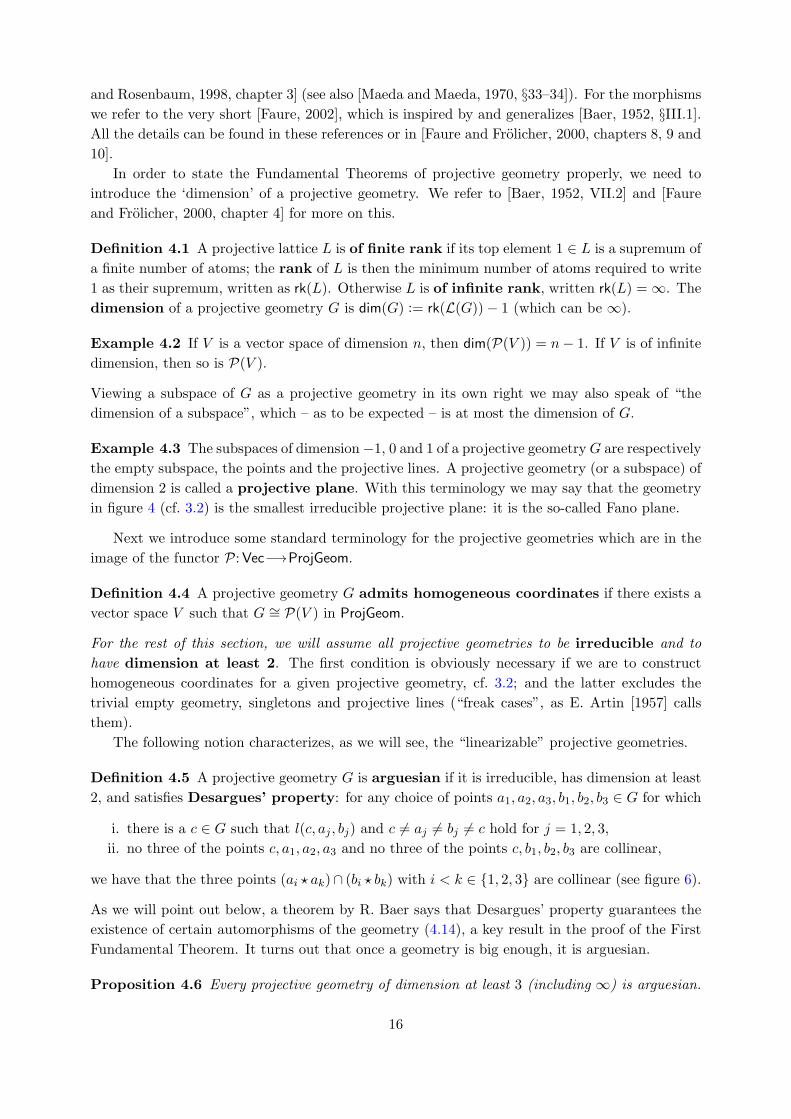
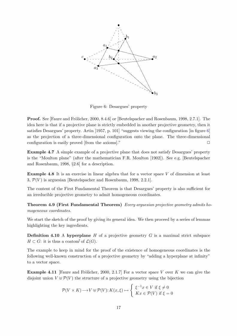
Definition 4.5 A projective geometry G is arguesian if it is irreducible, has dimension at least2, and satisfies Desargues’ property: for any choice of points a1, a2, a3, b1, b2, b3 ∈ G for which

i. there is a c ∈ G such that l(c, aj , bj) and c 6= aj 6= bj 6= c hold for j = 1, 2, 3,ii. no three of the points c, a1, a2, a3 and no three of the points c, b1, b2, b3 are collinear,

we have that the three points (ai ? ak)∩ (bi ? bk) with i < k ∈ {1, 2, 3} are collinear (see figure 6).

As we will point out below, a theorem by R. Baer says that Desargues’ property guarantees theexistence of certain automorphisms of the geometry (4.14), a key result in the proof of the FirstFundamental Theorem. It turns out that once a geometry is big enough, it is arguesian.

Proposition 4.6 Every projective geometry of dimension at least 3 (including ∞) is arguesian.

16

��

��

�

AAAAAAAAAAAAAA

XXXXXXXXXXXX

��

��

��l

ll

ll

ll

ll

ll

((((((((((((((• •

•

•

•

••

•

•

•c

a3

b3

a2

a1

b1

b2

Figure 6: Desargues’ property

Proof. See [Faure and Frolicher, 2000, 8.4.6] or [Beutelspacher and Rosenbaum, 1998, 2.7.1]. Theidea here is that if a projective plane is strictly embedded in another projective geometry, then itsatisfies Desargues’ property. Artin [1957, p. 101] “suggests viewing the configuration [in figure 6]as the projection of a three-dimensional configuration onto the plane. The three-dimensionalconfiguration is easily proved [from the axioms].” 2

Example 4.7 A simple example of a projective plane that does not satisfy Desargues’ propertyis the “Moulton plane” (after the mathematician F.R. Moulton [1902]). See e.g. [Beutelspacherand Rosenbaum, 1998, §2.6] for a description.

Example 4.8 It is an exercise in linear algebra that for a vector space V of dimension at least3, P(V ) is arguesian [Beutelspacher and Rosenbaum, 1998, 2.2.1].

The content of the First Fundamental Theorem is that Desargues’ property is also sufficient foran irreducible projective geometry to admit homogeneous coordinates.

Theorem 4.9 (First Fundamental Theorem) Every arguesian projective geometry admits ho-mogeneous coordinates.

We start the sketch of the proof by giving its general idea. We then proceed by a series of lemmashighlighting the key ingredients.

Definition 4.10 A hyperplane H of a projective geometry G is a maximal strict subspaceH ⊂ G: it is thus a coatom† of L(G).

The example to keep in mind for the proof of the existence of homogeneous coordinates is thefollowing well-known construction of a projective geometry by “adding a hyperplane at infinity”to a vector space.

Example 4.11 [Faure and Frolicher, 2000, 2.1.7] For a vector space V over K we can give thedisjoint union V ] P(V ) the structure of a projective geometry using the bijection

P(V ×K) // V ] P(V ):K(x, ξ) 7→

{ξ−1x ∈ V if ξ 6= 0Kx ∈ P(V ) if ξ = 0

17

Given an arguesian geometry G, we construct homogeneous coordinates G ∼= P(V ×K) ∼= V ]P(V ) by “recovering” the group of translations of the desired vector space V and its group ofhomotheties as certain collineations of G (i.e. isomorphisms from G to itself in ProjGeom) thatfix a chosen hyperplane (which will be P(V )).

Definition 4.12 A collineation α of G is called a central collineation if there is a hyperplaneH of G (the axis of α) and a point c ∈ G (the center of α) such that α fixes every point of Hand every line through c.

Central collineations are very rigid, as the following lemma shows.

Lemma 4.13 Let α be a central collineation of G with axis H and center c. Let p be a point inG \ ({c} ∪H). Then α is uniquely determined by α(p). In particular, for every x ∈ G not on H

nor on c ? p, we haveα(x) = (c ? x) ∩ (f ? α(p)) (5)

where f := (p ? x) ∩H.

Proof. See [Beutelspacher and Rosenbaum, 1998, 3.1.3] Note that α(x) ∈ c ? x because α hascenter c and α(x) ∈ f ? α(p) because x ∈ p ? x and α has axis H. These two lines intersect in apoint because they are distinct (as x 6∈ c ? p = c ? α(p)) and they lie in the plane spanned by p, xand c. 2

Here is the announced theorem where Desargues’ property comes into play.

Lemma 4.14 (Baer’s existence theorem of central collineations) Let G be arguesian. IfH is a hyperplane and c, p, p′ are distinct collinear points of G with p, p′ 6∈ H, then there is exactlyone collineation of G with center c and axis H mapping p to p′.

Proof. See [Beutelspacher and Rosenbaum, 1998, 3.1.8] or [Faure and Frolicher, 2000, 8.4.11].The basic idea is to use (5) to define the map. Desargues’ property is then used to show that itis well-defined and a collineation, through rather lengthy geometric verifications. 2

We now fix a hyperplane H of G and a point o ∈ G\H. Let T be the set of collineations withaxis H and center on H. We call an element of T a translation.

Lemma 4.15 T is an abelian group (under composition) which acts simply transitively on G\H.Translating this action of T into an addition on V := G \H, the latter also becomes an abeliangroup.

Proof. [Beutelspacher and Rosenbaum, 1998, 3.2.2] Simple transitivity of the action means thatif p 6= q in G\H then there is a unique collineation of G with axis H and center (p?q)∩H sendingp to q; it is a consequence of 4.14. The fact that T is a subgroup of the group of collineationsuses the fact that if a collineation has an axis, it has a center, and the rigidity of lemma 4.13.The commutativity of the group requires a little more work.

The simple transitivity allows us to transport the group structure from T to V . Indeed, forp ∈ V , denote τp the unique element in T such that τp(o) = p. For p, q ∈ V , we then put

p+ q := τp(q) = τp(τq(o)).

2

18

Next, let K× be the group (under composition) of all collineations of G with center o and axisH. We call an element of K× a homothety. It is an immediate consequence of 4.14 that K×

acts simply transitively on L \ {o} for every line L through o. Let αo be the constant morphismG //G: p 7→ o.

Lemma 4.16 If on the set K := K× ∪ {αo}, we define addition by

(σ1 + σ2)(x) := σ1(x) + σ2(x) for every x ∈ V

and multiplication by composition, then K becomes a field.

Proof. [Beutelspacher and Rosenbaum, 1998, 3.3.4] The main difficulty here is showing that Kis closed under this addition. 2

This multiplication is not commutative in general. Pappus’ Theorem geometrically characterizesthose arguesian geometries for which it is (see [Artin, 1957, chapter II, §7] for example).

Lemma 4.17 The action of K on V by

K × V // V : (σ, x) 7→ σ · x := σ(x)

is a “scalar multiplication” making V a (left) vector space over K.

Proof. [Beutelspacher and Rosenbaum, 1998, 3.3.5] Showing that σ(−x) = −σ(x) is whatrequires the most (but not that much) work. 2

The next lemma then finishes the proof of 4.9.

Lemma 4.18 G is isomorphic as a projective geometry to P(V ×K).

Proof. [Beutelspacher and Rosenbaum, 1998, 3.4.2] Remember that V = G\H. The isomorphismϕ:G //P(V ×K) is defined by

ϕ(x) :=

{K(x, 1) if x ∈ G\HK(y, 0) if x ∈ H, where y 6= x is any point of o ? x

which identifies H with P(V ) as expected. 2

Having dealt with objects, we move on to the linear representation of (some of) the morphismsof ProjGeom. Cl.-A. Faure [2002] has provided a short and elementary proof of the next theorem,which originally appeared in [Faure and Frolicher, 1994].

Theorem 4.19 (Second Fundamental Theorem) Let V1 and V2 be vector spaces. Everynon-degenerate morphism g:P(V1) //__ P(V2), meaning that its image contains three non-collinear points, is of the form P(f) for some semilinear map f :V1

// V2. Moreover f is uniqueup to scalar multiplication.

The uniqueness is an immediate consequence of the following fact (see e.g. [Faure, 2002, 2.4]),which we record here for future reference. Its proof is an exercise in linear algebra.

19

Proposition 4.20 Let f1, f2:V1// V2 be two additive maps between vector spaces (K1, V1) and

(K2, V2). Assume that f2(x) ∈ K2f1(x) for every x ∈ V1 and that f1(V1) contains two linearlyindependent vectors. Then there exists a µ ∈ K2 such that f2 = µf1.

The Second Fundamental Theorem implies that the vector space whose existence was guaranteedby the First Fundamental Theorem is essentially unique.

Corollary 4.21 If ϕ:P(V1) //P(V2) is an isomorphism in ProjGeom where V1 is a K1-vectorspace of dimension at least 3 and V2 is a K2-vector space (with K1,K2 fields), then there existsa field isomorphism σ:K1

//K2 and a bijective σ-linear map f :V1// V2 such that ϕ = P(f).

Remark that the uniqueness of homogeneous coordinates holds for projective dimension at least2 while existence needs dimension at least 3 (or Desargues’ property).

A composition of two non-degenerate morphisms need not be non-degenerate (think of thecomposition f ◦ g of two linear maps with img ⊆ kerf). A morphism of projective geometriesis called arguesian when it is the composite of finitely many non-degenerate morphisms. Thefollowing proposition [Faure and Frolicher, 2000, 10.3.1] says that these are exactly the morphismsinduced by semilinear maps.

Proposition 4.22 For a partial map g : P(V1) //__ P(V2) between arguesian geometries, the fol-lowing conditions are equivalent:

i. g is induced by a semilinear map f :V1// V2,

ii. g is the composite of two non-degenerate morphisms between arguesian geometries,iii. g is the composite of finitely many non-degenerate morphisms between arguesian geometries.

Proof. The only nontrivial implication is (i⇒ ii). Let σ be the field homomorphism associated tof . By hypothesis dim(V2) ≥ 3 and we can pick three linearly independent vectors y1, y2, y3 ∈ V2.Put W : = V1 ×K3

1 . Now define the maps

f1:V1//W :x 7→ (x, 0, 0, 0)

f2:W // V2 : (x, k1, k2, k3) 7→ f(x) + σ(k1)y1 + σ(k2)y2 + σ(k3)y3

Then f = f2 ◦ f1 and thus g = P(f) = P(f2) ◦ P(f1), where P(f1) and P(f2) are clearlynon-degenerate. 2

We define the category Arg of arguesian projective geometries and arguesian morphisms. TheFundamental Theorems may then be summarized in the following statement, which is as powerfulas one could hope.

Theorem 4.23 The functor P:Vecdim≥3// Arg is essentially surjective and essentially injective

on objects, full, and only identifies semilinear maps when they are a nonzero scalar multiple ofeach other.

5. Hilbert geometries, Hilbert lattices, propositional systems

A (real, complex, quaternionic or generalized) Hilbert spaceH is in particular a vector space, so by2.8 its one-dimensional linear subspaces form a projective geometry P(H). But the orthogonalityrelation on the elements of H, defined as x ⊥ y if and only if the inner product of x and y is

20

zero, obviously induces an orthogonality relation on P(H): A ⊥ B in P(H) when a ⊥ b for somea ∈ A \ {0} and b ∈ B \ {0}. We make an abstraction of this.

Definition 5.1 Given a binary relation ⊥ ⊆ G × G on a projective geometry G and a subsetA ⊆ G, we put A⊥ := {b ∈ G | ∀a ∈ A : b ⊥ a}. A Hilbert geometry G is a projective geometrytogether with an orthogonality relation ⊥ ⊆ G×G such that, for all a, b, c, p ∈ G,

(O1) if a ⊥ b then a 6= b,(O2) if a ⊥ b then b ⊥ a,(O3) if a 6= b, a ⊥ p, b ⊥ p and l(a, b, c) then c ⊥ p,(O4) if a 6= b then there is a q ∈ G such that l(q, a, b) and q ⊥ a,(O5) if S ⊆ G is a subspace such that S⊥⊥ = S, then S ∨ S⊥ = G.

Very often we shall simply speak of a “Hilbert geometry G”, leaving both the collinearity l andthe orthogonality ⊥ understood. A subspace S ⊆ G is said to be (biorthogonally) closed ifS⊥⊥ = S.

Axioms (O1–4) in the above definition say in particular that a Hilbert geometry is a ‘statespace’ in the sense of [Moore, 1995] as we explain in 8.2. The fifth axiom could have been writtenas: S = S⊥⊥ if and only if S ∨ S⊥ = G, because (as we shall show in 5.6 (iv) in a more abstractsetting) the necessity is always true. We make some more comments on these axioms in section8.

The term ‘Hilbert geometry’ is well-chosen, as C. Piron’s now famous example [1964, 1976]shows.

Definition 5.2 A generalized Hilbert space (also called orthomodular space) (H,K, ∗, 〈 , 〉)is a vector space H over a field K together with an involutive anti-automorphism K //K:α 7→ α∗

and an orthomodular Hermitian form H ×H //K: (x, y) 7→ 〈x, y〉, that is, a form satisfying

(S1) 〈λx1 + x2, y〉 = λ〈x1, y〉+ 〈x2, y〉 for all x1, x2, y ∈ H,λ ∈ K,(S2) 〈y, x〉 = 〈x, y〉∗ for all x, y ∈ H,

and such that, when putting S⊥ := {x ∈ H | ∀y ∈ S : 〈x, y〉 = 0} for a linear subspace S ⊆ H,

(S3) S = S⊥⊥ implies S ⊕ S⊥ = H.

Note that an orthomodular Hermitian form is automatically anisotropic,

(S4) 〈x, x〉 6= 0 for all x ∈ H \ {0},

and that in the finite dimensional case the converse is true too. I. Amemiya and H. Araki [1966]proved that when K is one of the “classical” fields equipped with its “classical” involution (Rwith identity, C and H with their respective conjugations), the definition of ‘generalized Hilbertspace’ is equivalent to the “classical” definition of a Hilbert space as inner-product space whichis complete for the metric induced by the norm. While H. Keller [1980] was the first to constructa “nonclassical” generalized Hilbert space, M. Soler [1995] proved that an infinite dimensionalgeneralized Hilbert space H is “classical” precisely when H contains an orthonormal sequence.We refer to [Holland, 1995] for a nice survey, and to A. Prestel’s [2006] contribution to thishandbook for a complete and historically annotated proof of Soler’s theorem. For a comment onthe lattice-theoretic meaning of Soler’s theorem, see 8.10.

21

Example 5.3 For a generalized Hilbert space H, the projective geometry P(H) together withthe obvious orthogonality relation forms a Hilbert geometry: axioms (O1–3) are immediate, (O4)follows from a standard Gram-Schmidt trick and (O5) is also immediate since S ∨ S⊥ = S ⊕ S⊥

for any linear subspace S of H.

From our work in section 2 we know that, since a Hilbert geometry is in particular a projectivegeometry, the lattice of subspaces L(H) is a projective lattice. Because of the orthogonalityrelation on G, there is some extra structure on L(G); the following proposition identifies it.

Proposition 5.4 If G is a Hilbert geometry with orthogonality relation ⊥, then the operator⊥:L(G) //L(G):S 7→ S⊥ satisfies, for all S, T ∈ L(G),

i. S ⊆ S⊥⊥,ii. if S ⊆ T then T⊥ ⊆ S⊥,iii. S ∩ S⊥ = ∅,iv. if S = S⊥⊥ and a ∈ G then {a} ∨ S = ({a} ∨ S)⊥⊥.v. if S = S⊥⊥ then S ∨ S⊥ = G.

Proof. All is straightforward, except for (iv). We need to prove that ({a} ∨ S)⊥⊥ ⊆ {a} ∨ S forS = S⊥⊥. If a ∈ S then this is trivial so we suppose from now on that a 6∈ S = S⊥⊥, i.e. thereexists p ∈ S⊥ such that a 6⊥ p. Let b ∈ ({a} ∨ S)⊥⊥; if b = a or b ∈ S then obviously b ∈ {a} ∨ S.If b 6= a and b 6∈ S then we claim that (a ? b) ∩ {p}⊥ is a singleton and moreover that its singleelement, call it q, belongs to S. This then proves the assertion, for q ⊥ p implies q 6= a, whichmakes q ∈ a ? b imply that b ∈ a ? q ⊆ {a} ∨ S.

Now (a ? b)∩{p}⊥ is non-empty4, because in case that a 6⊥ p 6⊥ b we can always pick x ∈ p ? aand y ∈ p ? b such that x, y ∈ {p}⊥ by (O4); then x 6= a and y 6= b so p ∈ (a ? x) ∩ (b ? y) and(G3) thus gives a q ∈ (a ? b) ∩ (x ? y) ⊆ (a ? b) ∩ {p}⊥ (for {p}⊥ is a subspace by (O3)). Wouldq1 6= q2 ∈ (a? b)∩{p}⊥, then l(q1, q2, a) by (G2) hence a ∈ {p}⊥, a contradiction. So we concludethat (a ? b) ∩ {p}⊥ = {q}.

We shall show that q ∈ S = S⊥⊥, i.e. for any r ∈ S⊥ we have q ⊥ r. For r = p this is true byconstruction; for r 6= p we may determine, by the “same” argument as above, a (unique) points ∈ {a}⊥ ∩ (p ? r) ⊆ ({a}⊥ ∩ S⊥) = ({a} ∨ S)⊥. The latter equality can be shown with a simplecalculation, but we also give a more abstract proof in 5.6 (iii). Because a, b ∈ ({a} ∨ S)⊥⊥ itfollows that a ⊥ s and b ⊥ s; hence we get q ⊥ s from q ∈ a ? b and (O3). But also s 6= p follows,thus s ∈ p ? r implies r ∈ p ? s, and because we know that q ⊥ p too, we finally obtain q ⊥ r,again from (O3). 2

This proposition calls for a new definition.

Definition 5.5 A projective lattice L is a Hilbert lattice if it comes with an orthogonalityoperator ⊥:L //L:x 7→ x⊥ satisfying, for all x, y ∈ L,

(H1) x ≤ x⊥⊥,(H2) if x ≤ y then y⊥ ≤ x⊥,(H3) x ∧ x⊥ = 0,

4What we really prove here is that for a, b, p with a 6= b in a Hilbert geometry G there always exists some q ∈ a?b

such that q ⊥ p. This statement, which is obviously stronger than (O4), is often used instead of (O4). See 8.3 for

a relevant comment.

22

(H4) if x = x⊥⊥ and a is an atom of L then a ∨ x = (a ∨ x)⊥⊥,(H5) if x = x⊥⊥ then x ∨ x⊥ = 1.

Usually we shall simply speak of “a Hilbert lattice L”, and leave the orthogonality operatorunderstood.

The crux of 5.4 is thus that the projective lattice of subspaces of a Hilbert geometry is aHilbert lattice. Having 2.10 in mind, it should not come as a surprise that there is a converseto this. However, we shall not give a direct proof of such a statement, for we wish to involveyet another mathematical structure. Again the source of inspiration is the concrete example ofHilbert spaces: the subspaces S ⊆ H for which S = S⊥⊥ are particularly important, for they areprecisely the subspaces which are closed for the norm topology on H (see [Schwartz, 1970, p. 392]for example). Also in the abstract case they are worth a closer look.

By a (biorthogonally) closed element of a Hilbert lattice (L, ⊥) we shall of course meanan x ∈ L for which x = x⊥⊥. We write C(L) ⊆ L for the ordered set of closed elements, withorder inherited from L. We shall now discuss some features of this ordered set that – as it willturn out – describe it completely. First we prove a technical lemma.

Lemma 5.6 For a Hilbert lattice L,

i. if x ∈ L then x⊥ ∈ C(L),ii. 0⊥⊥ = 0, 0⊥ = 1 and 1⊥ = 0,iii. (

∨i xi)⊥ =

∧i x

⊥i for (xi)i∈I ∈ L,

iv. if x ∨ x⊥ = 1 then x = x⊥⊥,v. the map ⊥⊥:L //L:x 7→ x⊥⊥ is a closure operator with fixpoints C(L).

Proof. Statements (i) and (ii) are almost trivial. For (iii) one uses (H1–2) over and again toverify ≥ and ≤ as follows:

∀k ∈ I :∧

i x⊥i ≤ x⊥k ∀k ∈ I : xk ≤

∨i xi

⇒ ∀k ∈ I : xk ≤ x⊥⊥k ≤ (∧

i x⊥i )⊥ ⇒ ∀k ∈ I : (

∨i xi)⊥ ≤ x⊥k

⇒∨

i xi ≤ (∧

i x⊥i )⊥ ⇒ (

∨i xi)⊥ ≤

∧i x

⊥i

⇒∧

i x⊥i ≤ (

∧i x

⊥i )⊥⊥ ≤ (

∨i xi)⊥

As for (iv), the assumption together with (H3) and modularity in L (for x ≤ x⊥⊥) give x =x ∨ 0 = x ∨ (x⊥ ∧ x⊥⊥) = (x ∨ x⊥) ∧ x⊥⊥ = 1 ∧ x⊥⊥ = x⊥⊥. Finally, it straightforwardly followsfrom (H2) that

ϕ:L // C(L):x 7→ x⊥⊥ and ψ: C(L) //L: y // y

are maps that preserve order, and they satisfy ϕ(x) ≤ y ⇔ x ≤ ψ(y) for any x ∈ L andy ∈ C(L). So these maps are adjoint, ϕ a ψ, and since moreover ϕ is surjective and ψ injective,the composition ψ ◦ ϕ:L //L:x 7→ x⊥⊥ is a closure operator with fixpoints C(L), as claimed in(v). 2

For closed elements (xi)i∈I ∈ L we shall write∨

ixi for (∨

i xi)⊥⊥, and in particular xOy for(x ∨ y)⊥⊥.

Proposition 5.7 For any Hilbert lattice L, the ordered set (C(L),≤) together with the restrictedoperator ⊥: C(L) // C(L):x 7→ x⊥ is a complete, atomistic, orthomodular† lattice satisfying thecovering law.

23

Proof. By (v) of 5.6, C(L) is a complete lattice inheriting infima from L, and with supremagiven by

∨. Moreover, (H2–3) assert that x 7→ x⊥ is an orthocomplementation† on C(L). It is

straightforward from (H4) and 5.6 (ii) that the atoms of L are closed; and conversely is it clearthat the atoms of C(L) are atoms of L too. So C(L) is atomistic, because L is. In the same way,since L has the covering law (cf. 2.9) and the atoms of L are precisely those of C(L), again (H4)assures that C(L) has the covering law too. Finally, if x ≤ y in C(L) then by the modular law inL and (H5)

xO(x⊥ ∧ y) = (x ∨ (x⊥ ∧ y))⊥⊥ = ((x ∨ x⊥) ∧ y)⊥⊥ = (1 ∧ y)⊥⊥ = y⊥⊥ = y;

i.e. the orthomodular law holds in C(L). 2

Example 5.8 By (H4) it follows that, if a1, ..., an are atoms of a Hilbert lattice L, then (eachone of them is closed and) a1O...Oan = a1 ∨ ... ∨ an. If L is a Hilbert lattice of finite rank, thenevery x ∈ L can be written as a finite supremum of atoms (this is true for any atomistic latticesatisfying the covering law of finite rank, see e.g. [Maeda and Maeda, 1970, section 8]), hencex = x⊥⊥; i.e. L ∼= C(L). So if G is a Hilbert geometry of finite dimension, then every subspace ofG is biorthogonally closed; in particular is this true for P(H) when H is a (generalized) Hilbertspace of finite dimension.

Inspired by the result in 5.7 we now give another definition due to C. Piron [1964, 1976].

Definition 5.9 An ordered set (C,≤) with an operator ⊥:C //C:x 7→ x⊥ is a propositionalsystem if it is a complete, atomistic, orthomodular lattice that satisfies the covering law (withx 7→ x⊥ as orthocomplementation).

We shall speak of “a propositional system C”, always using x⊥ as notation for the orthocomple-ment of x ∈ C. And we shall continue to write

∨ixi for the supremum in C, and

∧i xi for the

infimum.

Example 5.10 The closed subspaces of a generalized Hilbert space H form a propositionalsystem, that we shall write as C(H) instead of C(L(H)).

According to 5.7 and 5.9, the closed elements of a Hilbert lattice form a propositional system.Earlier we proved (cf. 5.4 and 5.5) that the subspaces of a Hilbert geometry form a Hilbert lattice.It is now time to come full circle: we want to associate a Hilbert geometry to a given propositionalsystem. The lattice-theoretical results in 2.9 will be useful here too.

Proposition 5.11 The set G(C) of atoms of a propositional system C form a Hilbert geometryfor collinearity and orthogonality given by

l(a, b, c) if a ≤ bOc or b = c, a ⊥ b if a ≤ b⊥. (6)

Proof. By definition C is complete, atomistic and satisfies the covering law; therefore it is uppersemimodular by (ii) of 2.9. But C is also orthocomplemented†, so it is isomorphic to its opposite†

(by C //Cop:x 7→ x⊥): upper semimodularity thus implies lower semimodularity. Then C musthave the intersection property by (iii) of 2.9, and so its atoms form a projective geometry for theindicated collinearity.

Now we must check the axioms for the orthogonality relation; the first three are (almost)trivial. For (O4), if a 6= b in G(C) then b ≤ aOa⊥ = 1 hence, by the intersection property,

24

(aOb) ∧ a⊥ 6= 0; the atomisticity of C gives us a q ∈ G(C) such that q ≤ aOb and q ≤ a⊥, aswanted. Finally, (O5) requires some more sophisticated calculations. First note that, for anysubspace S ⊆ G(C) and element a ∈ G(C),

a ∈ S⊥ ⇔ ∀b ∈ S : b ≤ a⊥ ⇔∨S ≤ a⊥ ⇔ a ≤ (

∨S)⊥.

Thus we always have that S⊥ = {a ∈ G(C) | a ≤ (∨S)⊥}, which by atomisticity of C means that∨

(S⊥) = (∨S)⊥; in particular is S closed, S = S⊥⊥, if and only if S = {a ∈ G(C) | a ≤

∨S}. If

S is a trivial subspace, then it is clear that S ∨S⊥ = G(C); so from now on, let S = S⊥⊥ be non-trivial. By the projective law, valid in L(G(C)) as in any other projective lattice, S ∨S⊥ = G(C)just means that for any p ∈ G(C) there exist a, b ∈ G(C) such that a ≤

∨S, b ≤ (

∨S)⊥ and

p ≤ aOb. And this is indeed true in the propositional system C; to simplify notations we shallwrite x :=

∨S in the argument that follows5. Suppose first that x ∧ (x⊥Op) 6≤ x⊥, then (by

C’s atomisticity) there must exist an a ∈ G(C) such that a ≤ x ∧ (x⊥Op) and a 6≤ x⊥. If a = p

then p ≤ x and we can pick any atom b ≤ x⊥ to show that p ≤ aOb as wanted. If a 6= p thenfrom a ≤ x⊥Op and the intersection property we get an atom b ≤ x⊥ ∧ (aOp); but certainlyis a 6= b (because a ≤ x and b ≤ x⊥) so b ≤ aOp is equivalent to p ≤ aOb by 2.9 (iv), aswanted. Next suppose that x∧ (x⊥Op) ≤ x⊥; this means that x⊥ = x⊥O(x∧ (x⊥Op)) = x⊥Op byorthomodularity in the second equality, so p ≤ x⊥. Picking any atom a ≤ x and putting b := p

we have p ≤ aOb as wanted. 2

Note that, for a given Hilbert lattice L, the atoms of C(L) are exactly those of L, and thesupremum of two atoms in C(L) is equal to their supremum in L. Thus it follows that G(C(L))(as in 5.11) is the same projective geometry as G(L) (as in 2.10).

Our aim is to build a triple categorical equivalence between Hilbert geometries, Hilbert latticesand propositional systems. We must therefore define an appropriate notion of ‘morphism betweenpropositional systems’. And then it turns out that we must restrict the morphisms betweenHilbert geometries, resp. Hilbert lattices, if we want to establish such a triple equivalence.

Definition 5.12 Let C1 and C2 be propositional systems. A map h:C1//C2 is a morphism

of propositional systems if it preserves arbitrary suprema and maps atoms of C1 to atoms orthe bottom element of C2.

It is a simple observation that propositional systems and their morphisms form a category PropSys.We shall now adapt the definition of ‘morphism’ between Hilbert geometries, resp. Hilbert

lattices: since these structures come with their respective closure operators, it is natural toconsider ‘continuous morphisms’.

Definition 5.13 Let G1 and G2 be Hilbert geometries. A morphism of projective geometriesg:G1

//__ G2 (as in 2.11) is continuous when, for every closed subspace F of G2, g∗(F ) is a closedsubspace of G1.

Let L1 and L2 be Hilbert lattices. A morphism of projective lattices f :L1//L2 (as in 2.14)

is continuous when f(x⊥⊥) ≤ f(x)⊥⊥ for every x ∈ L1.

Hilbert geometries and continuous morphisms form a category HilbGeom, and there is a faithfulfunctor HilbGeom // ProjGeom that “forgets” the orthogonality relation on a Hilbert geometry.

5This argument actually shows that for any p ∈ G(C) and any x ∈ C which is not 0 nor 1, there exist a, b ∈ G(C)

such that a ≤ x, b ≤ x⊥ and p ≤ aOb; see also [Maeda and Maeda, 1970, 30.7].

25

Similarly Hilbert lattices and continuous morphisms form a category HilbLat with a forgetfulfunctor to ProjLat.

Example 5.14 We say that a semilinear map f :H1//H2 between generalized Hilbert spaces

is continuous when it is so in the usual sense of the word with respect to biorthogonal closure.This is precisely saying that the induced morphism P(f):P(H1) //__ P(H2) is continuous in thesense of 5.13. There is then a category GenHilb of generalized Hilbert spaces and continuoussemilinear maps, and also a functor

P:GenHilb // HilbGeom:(f :H1

//H2

)7→

(P(f):P(H1) //__ P(H2)

).

The Second Fundamental Theorem 4.19 implies that every non-degenerate continuous morphismbetween Hilbert geometries P(H1) and P(H2) is induced by a continuous semilinear map.

In passing we note that the forgetful functor HilbGeom // ProjGeom is not full: there exist non-continuous linear maps between Hilbert spaces, and these induce non-continuous morphismsbetween (the underlying projective geometries of) Hilbert geometries.

The following is then the expected amendment of 2.15.

Proposition 5.15 If g:G1//__ G2 is a continuous morphism between Hilbert geometries then

L(g):L(G1) //L(G2):S 7→⋂{T ∈ L(G2) | S ⊆ g∗(T )}

is a continuous morphism between Hilbert lattices. If f :L1//L2 is a continuous morphism

between Hilbert lattices then its restriction to closed elements

C(f): C(L1) // C(L2):x 7→ f(x)⊥⊥

is a morphism of propositional systems. And if h:C1//C2 is a morphism between propositional

systems then

G(h):G(C1) //__ G(C2): a 7→ h(a) with kernel {a ∈ G(C1) | h(a) = 0}

is a continuous morphism between Hilbert geometries.

Proof. For a continuous morphism g:G1//__ G2 between Hilbert geometries and S ∈ L(G1) we

can compute, with notations as in 2.15, that

S ⊆ g∗(L(g)(S)

)⊆ g∗

((L(g)(S)

)⊥⊥)⇒ S⊥⊥ ⊆

(g∗

((L(g)(S)

)⊥⊥))⊥⊥= g∗

((L(g)(S)

)⊥⊥)⇒ L(g)(S⊥⊥) ⊆

(L(g)(S)

)⊥⊥because we know that L(g) a g∗ (used in the first and last line) and continuity of g:G1

//__ G2

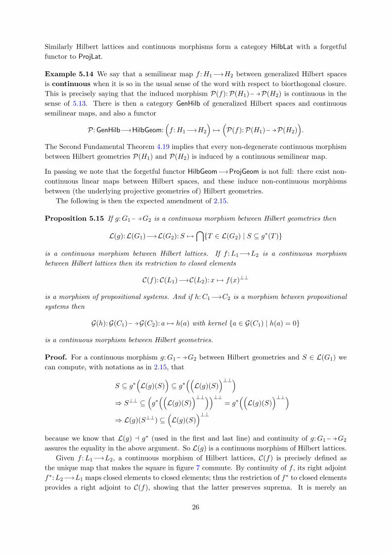
assures the equality in the above argument. So L(g) is a continuous morphism of Hilbert lattices.Given f :L1

//L2, a continuous morphism of Hilbert lattices, C(f) is precisely defined asthe unique map that makes the square in figure 7 commute. By continuity of f , its right adjointf∗:L2

//L1 maps closed elements to closed elements; thus the restriction of f∗ to closed elementsprovides a right adjoint to C(f), showing that the latter preserves suprema. It is merely an

26

L1f

//

( )⊥⊥

��

L2

( )⊥⊥

��

C(L1) C(f)// C(L2)

Figure 7: The definition of C(f)

observation that, because f sends atoms to atoms or 0, so does C(f). Thus C(f) is a morphismof propositional systems.

Finally, let h:C1//C2 be a morphism of propositional systems. From the proof of 5.11 we

know that a subspace S ⊆ G(C2) is closed if and only if S = {b ∈ G(C2) | b ≤∨S}; so in this

case

G(h)∗(S) = {a ∈ G(C1) | h(a) = 0} ∪ G(h)−1(S)

= {a ∈ G(C1) | h(a) ≤∨S}.

Writing h∗:C2//C1 for the right adjoint to h, this can be written as

G(h)∗(S) = {a ∈ G(C1) | a ≤ h∗(∨S)}

which shows that G(h)∗(S) is closed, since∨

(G(h)∗(S)) = h∗(∨S) by atomisticity. 2

Now we can conclude this section with the following result.

Theorem 5.16 The categories HilbGeom, HilbLat and PropSys are equivalent: the assignments

L:HilbGeom // HilbLat:(g:G1

//__ G2

)7→

(L(g):L(G1) //L(G2)

)C:HilbLat // PropSys:

(f :L1

//L2

)7→

(C(f): C(L1) // C(L2)

)G:PropSys // HilbGeom:

(h:C1

//C2

)7→

(G(h):G(C1) // G(C2)

)are functorial, and for a Hilbert geometry G, a Hilbert lattice L and a propositional system C

there are natural isomorphisms

κG:G ∼ // G(C(L(G))): a 7→ {a},λL:L ∼ //L(G(C(L))):x 7→ {a ∈ G(L) | a ≤ x},µC :C ∼ // C(L(G(C))):x 7→ {a ∈ G(C) | a ≤ x}.

Proof. We shall leave some verifications to the reader: the functoriality of G, L and C, and thenaturality of κ, λ and µ. But we shall prove that the latter are indeed isomorphisms.

Right after 5.11 we had already remarked that G(C(L(G))) = G(L(G)), i.e. C(L(G)) and L(G)have the same atoms and induce the same collinearity relation, so we already know by 2.16 thatκG is an isomorphism of projective geometries (it was called αG in 2.16); we only need to provethat κG and its inverse are continuous. A sufficient condition thereto is that two points a and

27

b of G are orthogonal if and only if κG(a) and κG(b) are orthogonal in G(C(L(G))). Indeed thisfact is true:

a ⊥ b⇔ a ∈ {b}⊥ ⇔ {a} ⊆ {b}⊥ ⇔ κG(a) ⊥ κG(b).

Similarly as above, we already know by 2.16 that λL is an isomorphism of projective lattices(it was called βL before). Now let a be an atom of C(L) (or of L) and x ∈ L, then

a ∈ λL(x⊥) ⇔ a ≤ x⊥∗⇔ x ≤ a⊥ ⇔ ∀b ∈ λL(x) : b ≤ a⊥ ⇔ a ∈ λL(x)⊥

(the equivalence in (∗) uses that the atom a is closed and that x ≤ x⊥⊥). This proves thatλL(x⊥) = λL(x)⊥ for all x ∈ L, from which it follows that λL and its inverse are continuousmorphisms of Hilbert lattices.

Finally, it is clear that each µC(x) ⊆ G(C) is a subspace (for the collinearity on G(C) as in5.11). Like before we have that µC(x⊥) = µC(x)⊥ for x ∈ C. It then follows easily that anysuch µC(x) is biorthogonally closed in L(G(C)), so at least is µC a well-defined, and obviouslyorder-preserving, map between ordered sets. The order-preserving map

ηC : C(L(G(C))) //C:S 7→∨S

satisfies ηC ◦ µC = idC by atomisticity of C; and in the proof of 5.11 we had already shown thata subspace S ⊆ G(C) is closed if and only if S = µC(ηC(S)), so µC ◦ ηC is the identity too. Thuswe find that µC and ηC constitute an isomorphism of lattices and hence µC is an isomorphism inPropSys, with inverse ηC . 2

The natural maps κG, λL and µC are actually more than isomorphisms in their respectivecategories: they are examples of ‘ortho-isomorphisms’. For completeness’ sake, we shall veryquickly make this precise.

Definition 5.17 A continuous morphism g:G1//__ G2 between Hilbert geometries is an ortho-

morphism if a ⊥ b implies g(a) ⊥ g(b) for every a, b in the domain of g. A continuous morphismf :L1

//L2 between Hilbert lattices is an ortho-morphism if f(x⊥) ≤ f(x)⊥ for all x ∈ L. Anda morphism h:C1

//C2 between propositional systems is an ortho-morphism if h(x⊥) ≤ h(x)⊥.

It obviously makes sense to consider the subcategories HilbGeom⊥, HilbLat⊥ and PropSys⊥ ofHilbGeom, HilbLat and PropSys with the same objects but with ortho-morphisms. An isomorphismin one of those categories is called a ortho-isomorphism. It turns out that the functors in 5.16restrict to these smaller categories, and we have actually shown in 5.16 that the maps κG, λL

and µC are ortho-isomorphisms: so the three categories HilbGeom⊥, HilbLat⊥ and PropSys⊥ areequivalent too.

It is also possible to consider ‘non-continuous ortho-morphisms’ between Hilbert geometriesG1 and G2, resp. Hilbert lattices L1 and L2: such is a morphism g:G1

//__ G2 in ProjGeom, resp.f :L1

//L2 in ProjLat, satisfying the appropriate orthogonality condition of 5.17. Two equivalentcategories are obtained, but it is not known if there is a third equivalent category of propositionalsystems, i.e. if there is a suitable notion of morphism between propositional systems to correspondwith that of ‘non-continuous ortho-morphism’ between Hilbert geometries, resp. Hilbert lattices.See [Faure and Frolicher, 2000, 14.3] for a discussion.

28

6. Irreducible components again

By “forgetting” about its orthogonality relation, we may view a Hilbert geometry G as an objectof ProjGeom and consider its decomposition in maximal irreducible subspaces, cf. 3.5. We shallshow that this coproduct actually “lives” in HilbGeom, but we must start off with a couple oflemmas. First an adaptation of 3.4: we prove that the functor HilbGeom // ProjGeom “creates”coproducts, from which it follows that HilbGeom has all coproducts and that the functor preservesthese.

Lemma 6.1 Given a family (Gi, li,⊥i)i∈I of Hilbert geometries, the coproduct of the underly-ing projective geometries (]iGi, l) in ProjGeom becomes a Hilbert geometry for the orthogonalityrelation

a ⊥ b if either a ∈ Gk, b ∈ Gl, k 6= l or a ⊥k b in some Gk,

and the inclusion morphisms (sk:Gk// ]i Gi)k∈I become continuous morphisms that form a

coproduct in HilbGeom.

Proof. First we verify axioms (O1–5) of 5.1, using the notations introduced there. Clearly (O1–2)are trivial. For (O3), if a, b both belong to some Gk, then also c ∈ Gk by the hypothesis l(a, b, c);if p 6∈ Gk then the conclusion holds trivially, and if p ∈ Gk then we may use (O3) in (Gk, lk,⊥k).If a, b belong to different components then c = a or c = b so that (O3) is trivially satisfied.The argument for (O4): if a ⊥ b then q := b does the job; if a 6⊥ b then a and b necessarilybelong to the same component Gk and we can apply (O4) to (Gk, lk,⊥k). The verification of(O5) is a bit more tricky. We already know from the proof of 3.4 that S ⊆ ]iGi is a subspaceof (]iGi, l) if and only if, for all k, S ∩ Gk is a subspace of (Gk, lk). Now an easy calculationshows that S⊥ ∩ Gk = (S ∩ Gk)⊥k , whence S⊥ = ]i(S⊥ ∩ Gi) = ]i(S ∩ Gi)⊥i and in particularS⊥⊥ = ]i(S ∩ Gi)⊥i⊥i . From this it follows that S is biorthogonally closed in G if and only if,for all k ∈ I, S ∩Gk is biorthogonally closed in Gk. In this case we can thus compute that:

S ∨ S⊥ =(]i (S ∩Gi)

)∨

(]i (S ∩Gi)⊥i

)∗= ]i

((S ∩Gi) ∨ (S ∩Gi)⊥i

)= ]iGi

= G.

The equation (∗) follows because the coproduct L(]iGi) ∼= ×iL(Gi) has the componentwise order.Since S ⊆ G is closed if and only if each S ∩Gk is closed, it is clear that each sk:Gk

// ]iGi

as in (3) is continuous: because s∗k(S) = S∩Gi. And for the same reason, the unique factorizationof a family of continuous morphisms (gk:Gk

//__ G) is easily seen to be continuous too: if S ⊆ G

is closed, then each g∗(S) ∩Gk = g∗k(S) ⊆ Gk is closed, so g∗(S) = ]ig∗i (S) ⊆ ]iGi is closed. 2

Recall that a subspace S ⊆ G of a projective geometry is always a projective geometry in itsown right (for the inherited collinearity), and that the inclusion S //G is always a morphism ofprojective geometries (with empty kernel). In the case of a Hilbert geometry G we can prove thatthe closure by biorthocomplement on G can be “relativized” to any of its closed subspaces.

Lemma 6.2 If S ⊆ G is a closed subspace of a Hilbert geometry, then S is a Hilbert geometry forthe inherited collinearity and orthogonality, and the inclusion S //G is a continuous morphismof Hilbert geometries.

29

Proof. In this proof we shall use the following notation: if T ⊆ S ⊆ G are subspaces with S

closed, we put T ′ := T⊥ ∩ S. We can prove a little trick:

T ′′ = (T⊥ ∩ S)⊥ ∩ S ∗= (T⊥⊥ ∨ S⊥) ∩ S ∗∗= T⊥⊥ ∨ (S⊥ ∩ S) = T⊥⊥. (7)

We used S = S⊥⊥ and 5.6 (iii) in (∗), and modularity of L(G) (or orthomodularity of C(L(G)),if one wishes) in (∗∗).

The verification of (O1–4) for the projective geometry S with inherited orthogonality is entirelystraightforward. As for (O5), let T ⊆ S be a subspace. Then (7) says that T ′′ = T impliesT⊥⊥ = T which implies T ∨ T⊥ = G, so that by modularity of L(G),

T ∨ T ′ = T ∨ (T⊥ ∩ S) = (T ∨ T⊥) ∩ S = S.

To verify the continuity of the morphism of projective geometries S ↪→ G, let T ⊆ G be aclosed subspace. The intersection of closed subspaces is always a closed subspace, so s∗(T ) = T∩Sis closed in G. But by (7) this is the same as being closed in S. 2

S. Holland [1995, 3.3] explains how this lemma can be seen as motivation for axiom (O5) in thedefinition of ‘Hilbert geometry’.

Finally we show a (remarkably strong) converse to 6.1.

Lemma 6.3 Given a family (Gi, li)i∈I of projective geometries, if their coproduct (]iGi, l) inProjGeom is in fact a Hilbert geometry for some orthogonality relation ⊥, then each (Gk, lk) be-comes a Hilbert geometry for the induced orthogonality, and the inclusion morphisms (sk:Gk

// ]i

Gi)k∈I become continuous morphisms that form a coproduct in HilbGeom.

Proof. By the above lemmas we only need to prove that the (Gi)i form a pairwise orthogonalfamily of closed subspaces of ]iGi. But let a ∈ Gj and b ∈ Gk for some j 6= k, then, by thecoproduct construction in ProjGeom, the line a ? b can only contain the points a and b, whichthus by (O4) of 5.1 must be orthogonal in the Hilbert geometry ]iGi. From this and (O1) it isthen easily seen that G⊥

j = ]i6=jGi, so that G⊥⊥j = Gj follows. 2

Having these technical results, we shall come to the point: we begin with a corollary of 3.5and the above lemmas.

Theorem 6.4 A Hilbert geometry G is the coproduct in HilbGeom of its maximal irreduciblesubspaces.

This now allows us to turn the elementary notion of ‘irreducibility’ for a Hilbert geometry into acategorical one by refining the result given in 3.6 for more general projective geometries.

Corollary 6.5 A Hilbert geometry G is irreducible (in the sense of 3.1 or equivalently 3.6) ifand only if it is not a coproduct in HilbGeom of two (or more) non-empty Hilbert geometries.

Proof. The coproduct-decompositions of a Hilbert geometry (G, l,⊥) in HilbGeom correspond tothose of the underlying projective geometry (G, l) in ProjGeom, by 6.1 and 6.3. 2

30

What the above really says, is that there is only one meaning for the term ‘irreducible Hilbertgeometry’ G, namely: all projective lines in G have at least three points, or equivalently: G isnot coproduct-decomposable in ProjGeom, or equivalently: G is not coproduct-decomposable inHilbGeom.

It is a matter of exploiting the categorical equivalence of Hilbert geometries and Hilbertlattices to deduce the following statements from the above and the results in section 3.

Lemma 6.6 The category HilbLat has coproducts. Explicitly, if (Li)i∈I are Hilbert lattices withrespective orthogonality operators x 7→ x⊥i, then the coproduct ×iLi in ProjLat becomes a Hilbertlattice for the orthogonality operator

(xi)i 7→ (x⊥ii )i,

and the inclusion morphisms sk:Lk// ×iLi become continuous morphisms that form a universal

cocone in HilbLat.

Proposition 6.7 A Hilbert lattice L is irreducible (in the sense of 3.9) if and only if it is not acoproduct in HilbLat of two (or more) non-trivial Hilbert lattices.

Proposition 6.8 Let G be a Hilbert geometry and L a Hilbert lattice that correspond to eachother under the equivalence HilbGeom ' HilbLat. Then L is irreducible if and only if G is.

Theorem 6.9 Every Hilbert lattice L is a coproduct in HilbLat of irreducible Hilbert lattices.

Finally we can state everything in terms of propositional systems; surely the reader is by nowfamiliar with our way of doing this, so we shall once again skip all the details.

Lemma 6.10 The category PropSys has coproducts. In fact, given a family (Ci)i∈I of proposit-ional systems with respective orthogonality operators x 7→ x⊥i, the cartesian product ×iCi withcomponentwise structure and the map

×iCi// ×i Ci: (xi)i 7→ (x⊥i

i )i

as orthocomplementation, is a propositional system; and the maps

sk:Ck// ×i Ci:x 7→ (xi)i

where xk = x and xi = 0 if i 6= k, form a universal cocone in PropSys.

Definition 6.11 A propositional system C is irreducible if it is not a coproduct in PropSys oftwo (or more) non-trivial propositional systems.

Proposition 6.12 Let G be a Hilbert geometry, L a Hilbert lattice and C a propositional systemthat correspond to each other under the triple equivalence HilbGeom ' HilbLat ' PropSys. ThenG is an irreducible Hilbert geometry if and only if L is an irreducible Hilbert lattice, if and onlyif C is an irreducible propositional system.

Theorem 6.13 Every propositional system C is the coproduct in PropSys of irreducible propo-sitional systems.

31

The remark that we have made at the end of section 3, can be repeated here: on the onehand can the statements in 6.9 and 6.13 be made more precise by saying exactly which are the“irreducible components” of a Hilbert lattice, resp. propositional system; on the other hand arethese theorems particular cases of a more general principle involving ‘central elements’ of lattices.Again we refer to 8.8 for a comment on this matter.

7. The Representation Theorem for propositional systems

This beautiful result is due to C. Piron [1964, 1976], who generalized the finite-dimensional versionof G. Birkhoff and J. von Neumann [1936].

Theorem 7.1 (Piron’s Representation Theorem) Every irreducible propositional system ofrank at least 4 is ortho-isomorphic to the lattice of (biorthogonally) closed subspaces of a gener-alized Hilbert space.

We can obviously put this theorem in geometric terms.

Theorem 7.2 For every arguesian Hilbert geometry (G,⊥) there exists a generalized Hilbertspace (H,K, ∗, 〈 , 〉) such that (G,⊥) is ortho-isomorphic to (P(H),⊥), where P(H) is given theorthogonality relation induced by 〈 , 〉.

Moreover, the Hermitian form of which this theorem speaks, is essentially unique.

Proposition 7.3 (Uniqueness of Hermitian form) Let H be a vector space over K. Letα 7→ α∗ and α 7→ α# be two involutions on K, let (x, y) 7→ 〈x, y〉 be a ∗-Hermitian form and(x, y) 7→ [x, y] a #-Hermitian form on H. If both Hermitian forms induce the same orthogonalityon P(H), then there exists 0 6= λ = λ∗ ∈ K such that ρ# = λ−1ρ∗λ for all ρ ∈ K and [x, y] =〈x, y〉λ for all x, y ∈ H.

The existence and uniqueness of a vector space with an anisotropic Hermitian form inducing theHilbert geometry (G,⊥) only require axioms (O1) through (O4) of the definition of a Hilbertgeometry (cf. 5.1). Axiom (O5) makes the Hermitian form orthomodular (see 8.4 and 8.5 forrelated comments). The field K in Theorem 7.2 cannot be finite [Eckmann and Zabey, 1969;Ivert and Sjodin, 1978]; see also [Faure and Frolicher, 2000, 14.1.12].

We shall now present S. Holland’s [1995, §3] proof of the geometric version of Piron’s theorem:it is essentially a smart application of the Second Fundamental Theorem to the isomorphisminduced by the orthogonality between G and its opposite geometry Gop. The latter is bydefinition G(Cop), where Cop is the propositional system opposite to C := C(L(G)) and it isthe isomorphism C ∼= Cop given by the orthocomplementation which induces the isomorphismG ∼= Gop. Geometrically, Gop has the closed hyperplanes {p⊥ | p ∈ G} as its points and itscollinearity satisfies, for p, q, r ∈ G,

l(p⊥, q⊥, r⊥) in Gop ⇔ l(p, q, r) in G⇔ q = r or p⊥ ⊇ q⊥ ∩ r⊥ in L(G). (8)

Given an arguesian Hilbert geometry G, we can by the First Fundamental Theorem assumethat G = P(H) for a K-vector space H. The dual

H∗ := {f :V //K | f linear}

32

is then a right K-vector space, thus a left vector space over the opposite field Kop (in which themultiplication, written with a centered dot, is reversed: ρ · λ = λρ). For every closed hyperplaneM = (Kx)⊥ of P(H) there exists a linear functional fx ∈ H∗, unique up to scalar multiple, whichhas M as its kernel. Now let F be the subspace of H∗ spanned by {fx | x ∈ H}.

Lemma 7.4 The map ϕ:P(H) //P(F ):Kx 7→ Kop · fx is an isomorphism of projective geome-tries.

Sketch of the proof. With (8) the lemma is proved by verifying that, for linear functionalsf, g, h ∈ H∗, f belongs to the Kop-span of g and h if and only if ker(f) ⊃ ker(g) ∩ ker(h); whichis an exercise in linear algebra [Faure and Frolicher, 2000, 11.1.11]. 2

Applying the Second Fundamental Theorem to the isomorphism ϕ, there exists a field isomor-phism σ:K //Kop and a bijective σ-linear map A:H //F such that ϕ(Kx) = Kop ·A(x) for allx ∈ H. Note that ker(A(y)) = (Ky)⊥.

Lemma 7.5 The map [ , ]:H×H //K: (x, y) 7→ [x, y] := A(y)(x) is sesquilinear: it is additivein both factors and satisfies for all x, y ∈ H and λ ∈ K

(Q1) [λx, y] = λ[x, y],(Q2) [x, λy] = [x, y]σ(λ).

Moreover, the orthogonality ⊥ on G = P(H) corresponds to the one induced by [ , ], that is,Kx ⊥ Ky ⇔ [x, y] = 0. Consequently, [ , ] is anisotropic (i.e. it satisfies (S4) right after 5.2).

All that is left is to find the involution on K and to rescale [ , ] to make it Hermitian. Because[ , ] is anisotropic we can choose a z ∈ H such that ε := [z, z] 6= 0. Define another sesquilinearform on H by putting 〈 , 〉 := [ , ]ε−1 and set ρ∗ := εσ(ρ)ε−1 for all ρ ∈ K. Then 〈 , 〉 inducesthe same orthogonality as [ , ] and it still satisfies (Q1) and (Q2) with σ replaced by the anti-automorphism ρ 7→ ρ∗ of K. To satisfy all requirements for (H,K, ∗, 〈 , 〉) to be a generalizedHilbert space (cf. 5.2) we now only need to prove a last result.

Lemma 7.6 For all x, y ∈ H and all ρ ∈ K, we have 〈x, y〉 = 〈y, x〉∗ and ρ∗∗ = ρ.

Proof. Apply 4.20 to the two maps H //F given by y 7→ 〈·, y〉 and y 7→ 〈y, ·〉#, where α 7→ α#

is the inverse automorphism of α 7→ α∗. Remembering that F is a Kop-vector space, we obtaina nonzero ξ ∈ K such that 〈x, y〉∗ = ξ∗〈y, x〉 for all x, y ∈ H. Then 1 = 〈z, z〉∗ = ξ∗〈z, z〉 = ξ∗

because 〈z, z〉 = 1. Moreover ρ = 〈ρz, z〉 = 〈z, ρz〉∗ = 〈ρz, z〉∗∗ = ρ∗∗〈z, z〉∗∗ = ρ∗∗, for everyρ ∈ K, proving that α 7→ α∗ is an involution on K. 2

This finishes the proof of 7.1 and 7.2. Uniqueness of the Hermitian form up to scaling (as statedin 7.3) is obtained by an application of 4.20.

In [Faure and Frolicher, 2000, §14.3] the reader can find representation theorems for morphismsbetween projective geometries preserving orthogonality, among which Wigner’s theorem whichgeometrically characterizes isometries for real, complex or hamiltonian Hilbert spaces. See also[Faure, 2002]. We state here a slightly more general but also well-known version.

Definition 7.7 LetH1 andH2 be orthomodular spaces over a fieldK. An isomorphism f :H1//H2

in Vec is called a semi-unitary if there exists a λ ∈ K such that for all x, y ∈ H1, we have〈f(x), f(y)〉 = σ(〈x, y〉)λ where σ:K //K is the automorphism associated to f . Moreover, f iscalled unitary when 〈f(x), f(y)〉 = 〈x, y〉 for all x, y ∈ H1.

33

Theorem 7.8 (Wigner) Let H1 and H2 be orthomodular spaces of dimension at least 3 overa field K. Then every ortho-isomorphism C(H1) // C(H2) is induced by a semi-unitary mapH1

//H2.

8. From here on

We shall end with some comments on the material that we presented in this chapter, and withsome hints for further study.

8.1 Projective closure. In a remark following 2.4 we have hinted at the fact that to any subsetA ⊆ G of a projective geometry we can associate the smallest subspace cl(A) ⊆ G that containsA. It is easily verified that this operation A 7→ cl(A) satisfies the following conditions:

i. it is monotone and satisfies cl(cl(A)) ⊆ cl(A) ⊇ A,ii. a ∈ cl(A) implies a ∈ cl(B) for some finite subset B ⊆ A,iii. x 6∈ cl(A) and x ∈ cl(A ∪ {b}) imply b ∈ cl(A ∪ {x}),iv. cl(∅) = ∅ and cl({a}) = {a} for all a ∈ G,v. for non-empty A,B ⊆ G, cl(A ∪B) =

⋃{cl({a, b}) | a ∈ cl(A), b ∈ cl(B)}.

A set G together with an operation cl: 2G // 2G satisfying (i) is called a closure space; if on topof that it satisfies (ii–iii) then it is a matroid. A closure space that also satisfies (iv) is a simpleclosure space; and a simple matroid is often called a geometry. If A 7→ cl(A) satisfies the wholelot (i–v) then it is a projective closure, and one can prove that any projective closure space(G, cl) is necessarily provided by a projective geometry. That is to say, there is an equivalence ofcategories ProjGeom ' ProjClos of projective geometries on the one hand and projective closurespaces on the other (with appropriate morphisms). But also the ‘weaker’ structures (matroids,geometries) are interesting in their own right; in particular can a whole deal of “dimension theory”for projective geometries (cf. 4.1) be carried out for structures as basic as matroids. This is thesubject of Cl.-A. Faure and A. Frolicher’s [1996], see also their [2000, chapters 3 and 4].

8.2 State spaces and property lattices. In the definition 5.1 of Hilbert geometry, it followsfrom (O1–4) that a Hilbert geometry is a state space in the sense of [Moore, 1995]: if a 6= b

then l(q, a, b) and q ⊥ a for some q ∈ G by (O4), but would q ⊥ b as well then q ⊥ q by (O2–3)(and the symmetry of l) which is excluded by (O1). That is to say, the relation ⊥ is irreflexive,symmetric and separating (in the sense that a 6= b implies the existence of some q such thata ⊥ q 6⊥ b). Moore [1995] proves that the biorthogonally closed subspaces of a state space form aso-called property lattice: a complete, atomistic and orthocomplemented lattice. Of course, apropositional system (cf. 5.9) is a particular example of such a ‘property lattice’. More precisely,state spaces and property lattices are the objects of equivalent categories State and Prop of whichthe equivalence of HilbGeom with PropSys is a restriction. For the relevance of State and Prop intheoretical physics see [Moore, 1999].

8.3 Fewer axioms for geometries with orthogonality. F. Buekenhout [1993] explains howA. Parmentier and he showed that, remarkably, (G3) of 2.1 is automatically true for a set G witha collinearity l satisfying just (G1–2) and an orthogonality ⊥ satisfying (cf. 5.1)

(O2) if a ⊥ b then b ⊥ a,(O3) if a 6= b, a ⊥ p, b ⊥ p and c ∈ a ? b then c ⊥ p,

34

(O6) if a, b, p ∈ G and a 6= b then there is a q ∈ a ? b with q ⊥ p,(O7) for all a ∈ G there is a b ∈ G with a 6⊥ b.

Clearly, (O1) implies (O7), and in the proof of 5.4 we have shown that (O6) too is valid in anyHilbert geometry.

8.4 Geometries “with extra structure”. A Hilbert geometry is, by 5.1, a projective geometrywith extra structure—a lot of extra structure, actually. There are many notions of ‘projectivegeometry with extra structure’ that are weaker than Hilbert geometries but still have manyinteresting properties. A large part of [Faure and Frolicher, 2000] is devoted to the study of suchthings as Mackey geometries, regular Mackey geometries, orthogeometries and pureorthogeometries: structures that lie between projective geometries and Hilbert geometries.Several of these ‘geometries with extra structure’ can be represented by appropriate ‘vector spaceswith extra structure.’ In that spirit, [Holland, 1995, 3.6] and [Faure and Frolicher, 2000, 14.1.8]are slight generalizations of Piron’s representation theorem (cf. 7.1 and 7.2) which include skew-symmetric forms.

8.5 On orthomodularity. Given a vector space V with an anisotropic Hermitian form (i.e.a form satisfying (S1, S2 and S4) in 5.2) and induced orthogonality ⊥ we have that (P(V ),⊥)satisfies (O5) if and only if L(V ) satisfies (H5) if and only if the lattice of closed subspace C(V )is orthomodular if and only if the Hermitian form satisfies (S3). In other words, and this is a keyinsight of Piron’s [1964], orthomodularity of C(V ) is what distinguishes the generalized Hilbertspaces among the (anisotropic) Hermitian spaces. This is one of the reasons why orthomodularlattices have been heavily studied; the standard reference on the subject is [Kalmbach, 1983].

8.6 Projectors. For a projective geometry G together with a binary relation ⊥ on G thatsatisfies (O1–4) in 5.1, a (necessarily closed, cf 5.6) subspace S ⊆ G satisfies S ∨ S⊥ = G if andonly if for every a ∈ G\S⊥ the subspace ({a}∨S⊥)∩S is non-empty. In this case, ({a}∨S⊥)∩Sis a singleton, and writing r(a) for its single element gives a partial map

r:G //__ S: a 7→ r(a) with kernel S⊥

which is a retract to the inclusion i:S //G.

Proof. Suppose that S ∨ S⊥ = G and that a ∈ G \ (S ∪ S⊥) (if a ∈ S then all is trivial). Bythe projective law, a ∈ x ? y for some x ∈ S and y ∈ S⊥, whence x ∈ a ? y ⊆ {a} ∨ S⊥, sox ∈ ({a}∨S⊥)∩S 6= ∅. Conversely, suppose that a ∈ G \ (S ∪S⊥). Pick any x ∈ ({a}∨S⊥)∩S:thus x ∈ S and x ∈ a ? y for some y ∈ S⊥, whence a ∈ x ? y ⊆ S ∨ S⊥ (using the projective lawtwice), which proves that S ∨ S⊥ = G.

Would x1, x2 be different elements of ({a}∨S⊥)∩S for some a 6∈ S⊥, then x1, x2 ∈ S and thereexist y1, y2 ∈ {a}∨S⊥ such that xi ∈ a ? yi for i = 1, 2. Because a 6∈ S⊥, a is necessarily differentfrom the yi’s. But a is also different from the xi’s: if a = x1 for example, then x2 ∈ x1 ? y2 fromwhich y2 ∈ x1 ? x2 ⊆ S, which is impossible since S ∩ S⊥ = ∅ by (O1). So we can equivalentlywrite that a ∈ (x1 ?y1)∩ (x2 ?y2); and by axiom (G3) of 2.1 we get a point b ∈ (x1 ?x2)∩ (y1 ?y2).But such b lies in both S and S⊥, which is impossible. Hence the non-empty set ({a} ∨ S⊥) ∩ Sis a singleton. In particular does this argument imply that {a} = ({a} ∨ S⊥)∩ S if a ∈ S: so thepartial map r:G //__ S sending a 6∈ S⊥ to the single element of ({a} ∨ S⊥) ∩ S is a retract to theinclusion i:S //G. 2

35

Now i:S //G is a morphism of projective geometries when we let S inherit the collinearity fromG, but in fact so is r:G //__ S. Therefore pr := i ◦ r:G //__ G is an idempotent morphism ofprojective geometries with kernel S⊥ and image S. It is moreover true that pr(a) ⊥ b⇔ a ⊥ pr(b)for a, b 6∈ S⊥ (the morphism is “self-adjoint”), and so we have every reason to speak of theprojector with image S and kernel S⊥. Much more on this can be found in [Faure and Frolicher,2000, section 14.4].

8.7 More on projectors. Interestingly, there is a lattice-theoretic analog of 8.6: A com-plete orthocomplemented lattice C is orthomodular if and only if for each x ∈ C the mapϕx:C //C: y 7→ x∧(x⊥∨y) has a right adjoint, which then is the map ψx:C //C: y 7→ x⊥∨(x∧y).If C is moreover atomistic and satisfies the covering law, then ϕx is a morphism of propositionalsystems.

Proof. Clearly the maps ϕx and ψx preserve order. Now let C be a complete orthocomplementedorthomodular lattice, then

ψx(ϕx(y)) = x⊥ ∨(x ∧ (x ∧ (x⊥ ∨ y))

)= x⊥ ∨

(x ∧ (x⊥ ∨ y)

)∗= x⊥ ∨ y ≥ y

where orthomodularity was used in (∗). Similarly one shows ϕx(ψx(y)) ≤ y, so we get theadjunction ϕx a ψx. Conversely, if x ≤ y in a complete orthocomplemented lattice C, then usingthis information in (∗∗) gives

ϕx⊥(y) = x⊥ ∧ (x⊥⊥ ∨ y) = x⊥ ∧ (x ∨ y) ∗∗= x⊥ ∧ y ≤ y,

ψx⊥(y) = x⊥⊥ ∨ (x⊥ ∧ y) = x ∨ (x⊥ ∧ y)∗∗≤ y ∨ y = y.

Assuming that ϕx⊥ a ψx⊥ we get y ≤ ψx⊥(y) from the first line, thus y = ψx⊥(y) if we combineit with the second line, which is the orthomodular law.

Next suppose that C is a propositional system, let a ∈ C be an atom and x ∈ C. If a ≤ x⊥

then ϕx(a) = 0. If a 6≤ x⊥ then a ∧ x⊥ = 0 so x⊥ l a ∨ x⊥. By lower semimodularity of C (see5.11 and use [Faure and Frolicher, 2000, 1.5.7]) it follows that either x ∧ x⊥ = x ∧ (a ∨ x⊥) orx ∧ x⊥ l x ∧ (a ∨ x⊥); in any case we have shown that ϕx(a) is 0 or covers 0. 2

A map like the ϕx:C //C in the statement above, is called a Sasaki projector, and its rightadjoint is a Sasaki hook. These maps were introduced by U. Sasaki [1954], and extensively usedin [Piron, 1976, 4–1] to describe lattice-theoretically the effect of an “ideal measurement of thefirst kind” on a (quantum) physical system. See also [Coecke and Smets, 2004] for a discussionof the (quantum logical) meaning of the adjunction of Sasaki projection and Sasaki hook.

8.8 Another irreducibility criterion. A bounded lattice is, by definition, a lattice witha smallest element 0 and a greatest element 1. If L1 and L2 are bounded lattices then, withcomponentwise lattice structure, the cartesian product L1 × L2 is a bounded lattice too. Anelement z ∈ L of a bounded lattice is central if there exist bounded lattices L1, L2 and anisomorphism (i.e. a bijection that preserves and reflects order) ϕ:L1 × L2

∼ //L such that z =ϕ(1, 0). The set Z(L) of central elements, called the center of L, is an ordered subset of L thatcontains at least 0 and 1. A wealth of information on this topic can be found in [Maeda andMaeda, 1970, sections 4 and 5] or any other standard reference on lattice theory.

One can easily figure out that the cartesian product L1×L2 of bounded lattices is a projectivelattice if and only if L1 and L2 are projective lattices (just view such an Li as a segment in L);

36

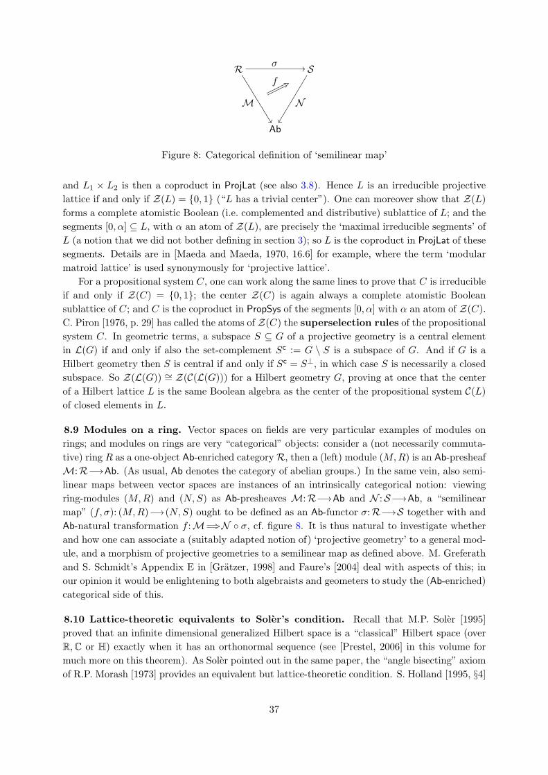
f 3;oooooooooo

R σ //

M��

3333

3333

3333

3 S

N����

����

����

��

Ab

Figure 8: Categorical definition of ‘semilinear map’

and L1 × L2 is then a coproduct in ProjLat (see also 3.8). Hence L is an irreducible projectivelattice if and only if Z(L) = {0, 1} (“L has a trivial center”). One can moreover show that Z(L)forms a complete atomistic Boolean (i.e. complemented and distributive) sublattice of L; and thesegments [0, α] ⊆ L, with α an atom of Z(L), are precisely the ‘maximal irreducible segments’ ofL (a notion that we did not bother defining in section 3); so L is the coproduct in ProjLat of thesesegments. Details are in [Maeda and Maeda, 1970, 16.6] for example, where the term ‘modularmatroid lattice’ is used synonymously for ‘projective lattice’.

For a propositional system C, one can work along the same lines to prove that C is irreducibleif and only if Z(C) = {0, 1}; the center Z(C) is again always a complete atomistic Booleansublattice of C; and C is the coproduct in PropSys of the segments [0, α] with α an atom of Z(C).C. Piron [1976, p. 29] has called the atoms of Z(C) the superselection rules of the propositionalsystem C. In geometric terms, a subspace S ⊆ G of a projective geometry is a central elementin L(G) if and only if also the set-complement Sc := G \ S is a subspace of G. And if G is aHilbert geometry then S is central if and only if Sc = S⊥, in which case S is necessarily a closedsubspace. So Z(L(G)) ∼= Z(C(L(G))) for a Hilbert geometry G, proving at once that the centerof a Hilbert lattice L is the same Boolean algebra as the center of the propositional system C(L)of closed elements in L.

8.9 Modules on a ring. Vector spaces on fields are very particular examples of modules onrings; and modules on rings are very “categorical” objects: consider a (not necessarily commuta-tive) ring R as a one-object Ab-enriched categoryR, then a (left) module (M,R) is an Ab-presheafM:R // Ab. (As usual, Ab denotes the category of abelian groups.) In the same vein, also semi-linear maps between vector spaces are instances of an intrinsically categorical notion: viewingring-modules (M,R) and (N,S) as Ab-presheaves M:R // Ab and N :S // Ab, a “semilinearmap” (f, σ): (M,R) // (N,S) ought to be defined as an Ab-functor σ:R // S together with andAb-natural transformation f :M +3N ◦ σ, cf. figure 8. It is thus natural to investigate whetherand how one can associate a (suitably adapted notion of) ‘projective geometry’ to a general mod-ule, and a morphism of projective geometries to a semilinear map as defined above. M. Greferathand S. Schmidt’s Appendix E in [Gratzer, 1998] and Faure’s [2004] deal with aspects of this; inour opinion it would be enlightening to both algebraists and geometers to study the (Ab-enriched)categorical side of this.

8.10 Lattice-theoretic equivalents to Soler’s condition. Recall that M.P. Soler [1995]proved that an infinite dimensional generalized Hilbert space is a “classical” Hilbert space (overR,C or H) exactly when it has an orthonormal sequence (see [Prestel, 2006] in this volume formuch more on this theorem). As Soler pointed out in the same paper, the “angle bisecting” axiomof R.P. Morash [1973] provides an equivalent but lattice-theoretic condition. S. Holland [1995, §4]

37

used “harmonic conjugates” to formulate another lattice-theoretic alternative. He also proposed[Holland, 1995, §5] a (non lattice-theoretic) “ample unitary group axiom”: an infinite dimensionalorthomodular space H over K is a “classical” Hilbert space if and only if for any two orthogonalnonzero vectors a, b ∈ H there exists a unitary map U : H //H (see 7.7) such that U(Ka) = Kb.R. Mayet [1998] has proved the following lattice-theoretic alternative: an orthomodular spaceH is an infinite dimensional Hilbert space over R,C or H if and only if there exist a, b ∈ C(H)where dim b ≥ 2 and an ortho-isomorphism f : C(H) // C(H) such that f |[0,b] is the identicalmap and f(a) � a. The condition on f |[0,b] guarantees that the semi-unitary map inducing f (byWigner’s theorem, see 7.8) is unitary. Similar characterizations using “symmetries” of the latticeC(H) were proposed in [Aerts and Van Steirteghem, 2000] and in [Engesser and Gabay, 2002].The question whether the transitivity of the whole group of ortho-isomorphisms of C(H) stillcharacterizes the “classical” Hilbert spaces among the infinite dimensional orthomodular spacesseems to be unanswered.

9. Appendix: notions from lattice theory

Mostly to fix terminology, we recall the notions from lattice theory we have used in this chapter;in the previous sections these are marked with a “†” when they are used for the first time.

A partially ordered set, also called simply ordered set or poset, is a set P together witha binary relation ≤ which is reflexive, antisymmetric and transitive. We also use the standardnotation x < y for x ≤ y and x 6= y. The opposite ordered set P op has the same elements as Pbut with its order relation 4 reversed: for x, y ∈ P we have x ≤ y ⇔ y 4 x.

For a subset X of P we say that p ∈ P is an upper bound of X if x ≤ p for every x ∈ X, wesay that p is a least upper bound, or a supremum, or a join, of X if for every other upperbound q we have p ≤ q. By antisymmetry a least upper bound is unique if it exists. The conceptof greatest lower bound (also called infimum or meet) is defined dually. If the supremum ofX exists and lies in X we call it the maximum of X, denoted by maxX. Dually, we can defineminX, the minimum of X.

A lattice is a poset L any two of whose elements x, y ∈ L have a meet denoted by x ∧ yand a join denoted by x ∨ y. It is complete if any subset X ⊆ L has a join, then denoted by∨X, and a meet

∧X. (In fact, if all joins exist in an ordered set L then so do all meets, and

vice versa; thus an ordered set L is a complete lattice if and only if it has all joins, if and only ifit has all meets.) Putting X = L we see that a complete lattice has a bottom element 0 and atop element 1, that is, elements satisfying 0 ≤ x ≤ 1 for every x ∈ L. For a ≤ b in a lattice L,the interval or segment [a, b] is the lattice {x ∈ L | a ≤ x ≤ b}.

A map f :P1//P2 between two ordered sets is said to preserve order, or is called mono-

tone, if for any x, y ∈ P1,x ≤ y implies f(x) ≤ f(y).

It is an isomorphism of ordered sets (or of lattices when appropriate) if it moreover has anorder-preserving inverse.

For two elements x, y of P we say that y covers x and we write xl y when x < y but neverx < p < y for p ∈ P . If P is a poset with bottom element 0, we call a ∈ P an atom if acovers 0. If P is a poset with top element 1 then c is a coatom if 1 covers c. A lattice L withbottom element 0 is called6 atomistic if every element x ∈ L is the join of the atoms it contains:

6G. Birkhoff [1967] calls these ‘atomic’ or ‘point lattices’.

38

x =∨{a ∈ L | a atom, a ≤ x}.

A nonempty subset D ⊆ P of a poset is called directed if for any x, y ∈ D, there existsz ∈ D such that x ≤ z and y ≤ z. A complete lattice L is called continuous (some say meet-continuous) if for any directed set D ⊆ L and any a ∈ L we have a∧ (

∨D) =

∨{a∧ d | d ∈ D}.

A lattice L is called modular if, for every x, y, z ∈ L,

x ≤ z implies x ∨ (y ∧ z) = (x ∨ y) ∧ z.

The following are weaker notions: L is upper semimodular if u ∧ v l v implies ul u ∨ v; andit is lower semimodular if ul u ∧ v implies u ∧ v l v.

A lattice L with 0 satisfies the covering law if for any x ∈ L and any atom a ∈ L we have

a ∧ x = 0 implies xl a ∨ x.

An orthocomplementation on a lattice L with 0 and 1 is a map L //L:x 7→ x⊥ whichsatisfies, for all x, y ∈ L,

i. x ≤ y implies y⊥ ≤ x⊥,ii. (x⊥)⊥ = x,iii. x ∨ x⊥ = 1 and x ∧ x⊥ = 0.

A lattice is called orthocomplemented if it is equipped with an orthocomplementation. Sucha lattice L is called orthomodular if moreover, for all x, y ∈ L,

x ≤ y implies x ∨ (x⊥ ∧ y) = y.

Since the orthocomplementation induces an isomorphism L //Lop

this is equivalent to

x ≤ y implies y ∧ (y⊥ ∨ x) = x.

Given two order-preserving maps f :P1//P2 and g:P2

//P1 in opposite directions, we saythat f is a left adjoint of g, and g a right adjoint of f , written f a g, if they satisfy one, andhence all, of the following equivalent conditions:

i. for all x ∈ P1 and y ∈ P2 we have f(x) ≤ y ⇔ x ≤ g(y),ii. f(x) = min{y ∈ P2 | x ≤ g(y)} for all x ∈ P1,iii. g(y) = max{x ∈ P1 | f(x) ≤ y} for all y ∈ P2,iv. x ≤ g(f(x)) and f(g(y)) ≤ y for all x ∈ P1 and all y ∈ P2.

The pair (f, g) is called a Galois connection or said to form an adjunction (between theordered sets P1 and P2.) It follows from conditions (ii) and (iii) above that adjoints determineeach other uniquely (when they exist). And one can check that f is surjective if and only if g isinjective, if and only if f(g(y)) = y for all y ∈ P2.

Still considering such an adjunction f a g, f preserves all joins that exist in P1; similarly, gpreserves all meets that exist in P2. Conversely, for an ordered set L the following conditions areequivalent:

i. L is a complete lattice,ii. every map h:L //P preserving all joins has a right adjoint,iii. every map h:L //Q preserving all meets has a left adjoint.

39

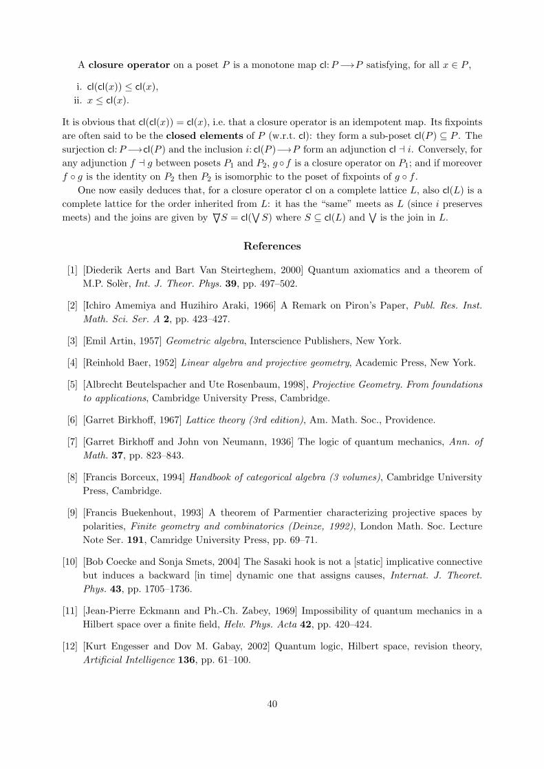
A closure operator on a poset P is a monotone map cl:P //P satisfying, for all x ∈ P ,

i. cl(cl(x)) ≤ cl(x),ii. x ≤ cl(x).

It is obvious that cl(cl(x)) = cl(x), i.e. that a closure operator is an idempotent map. Its fixpointsare often said to be the closed elements of P (w.r.t. cl): they form a sub-poset cl(P ) ⊆ P . Thesurjection cl:P // cl(P ) and the inclusion i: cl(P ) //P form an adjunction cl a i. Conversely, forany adjunction f a g between posets P1 and P2, g ◦f is a closure operator on P1; and if moreoverf ◦ g is the identity on P2 then P2 is isomorphic to the poset of fixpoints of g ◦ f .

One now easily deduces that, for a closure operator cl on a complete lattice L, also cl(L) is acomplete lattice for the order inherited from L: it has the “same” meets as L (since i preservesmeets) and the joins are given by

∨S = cl(

∨S) where S ⊆ cl(L) and

∨is the join in L.

References

[1] [Diederik Aerts and Bart Van Steirteghem, 2000] Quantum axiomatics and a theorem ofM.P. Soler, Int. J. Theor. Phys. 39, pp. 497–502.

[2] [Ichiro Amemiya and Huzihiro Araki, 1966] A Remark on Piron’s Paper, Publ. Res. Inst.Math. Sci. Ser. A 2, pp. 423–427.

[3] [Emil Artin, 1957] Geometric algebra, Interscience Publishers, New York.

[4] [Reinhold Baer, 1952] Linear algebra and projective geometry, Academic Press, New York.

[5] [Albrecht Beutelspacher and Ute Rosenbaum, 1998], Projective Geometry. From foundationsto applications, Cambridge University Press, Cambridge.

[6] [Garret Birkhoff, 1967] Lattice theory (3rd edition), Am. Math. Soc., Providence.

[7] [Garret Birkhoff and John von Neumann, 1936] The logic of quantum mechanics, Ann. ofMath. 37, pp. 823–843.

[8] [Francis Borceux, 1994] Handbook of categorical algebra (3 volumes), Cambridge UniversityPress, Cambridge.

[9] [Francis Buekenhout, 1993] A theorem of Parmentier characterizing projective spaces bypolarities, Finite geometry and combinatorics (Deinze, 1992), London Math. Soc. LectureNote Ser. 191, Camridge University Press, pp. 69–71.

[10] [Bob Coecke and Sonja Smets, 2004] The Sasaki hook is not a [static] implicative connectivebut induces a backward [in time] dynamic one that assigns causes, Internat. J. Theoret.Phys. 43, pp. 1705–1736.

[11] [Jean-Pierre Eckmann and Ph.-Ch. Zabey, 1969] Impossibility of quantum mechanics in aHilbert space over a finite field, Helv. Phys. Acta 42, pp. 420–424.

[12] [Kurt Engesser and Dov M. Gabay, 2002] Quantum logic, Hilbert space, revision theory,Artificial Intelligence 136, pp. 61–100.

40

[13] [Claude-Alain Faure, 2002] An elementary proof of the fundamental theorem of projectivegeometry, Geom. Ded. 90, pp. 145–151.

[14] [Claude-Alain Faure, 2004] Morphisms of projective spaces over rings, Adv. Geom. 4, pp. 19–31.

[15] [Claude-Alain Faure and Alfred Frolicher, 1993] Morphisms of projective geometries and ofcorresponding lattices, Geom. Ded. 47, pp. 25–40.

[16] [Claude-Alain Faure and Alfred Frolicher, 1994] Morphisms of Projective Geometries andSemilinear Maps, Geom. Ded. 53, pp. 237–262.

[17] [Claude-Alain Faure and Alfred Frolicher, 1995] Dualities for Infinite-Dimensional ProjectiveGeometries, Geom. Ded. 56, pp. 225–236.

[18] [Claude-Alain Faure and Alfred Frolicher, 1996] The dimension theorem in axiomatic geom-etry, Geom. Ded. 60, pp. 207–218.

[19] [Claude-Alain Faure and Alfred Frolicher, 2000] Modern projective geometry, Kluwer Aca-demic Publishers, Dordrecht.

[20] [George Gratzer, 1998] General lattice theory (2nd edition), Birkhauser Verlag, Basel.

[21] [Samuel S. Holland, Jr., 1995] Orthomodularity in infinite dimensions; a theorem of M. Soler,Bull. Amer. Math. Soc. 32, pp. 205–234.

[22] [Per-Anders Ivert and Torgny Sjodin, 1978] On the impossibility of a finite propositionalsystem for quantum mechanics, Helv. Phys. Acta 51, pp. 635–636.

[23] [Gudrun Kalmbach, 1983] Orthomodular lattices, London Mathematical Society Monographs18, Academic Press Inc., London.

[24] [Hans Arwed Keller, 1980] Ein nicht-klassicher Hilbertscher Raum, Math. Z. 172, pp. 41–49.

[25] [Saunders Mac Lane, 1971] Categories for the working mathematician, Springer-Verlag, NewYork.

[26] [Fumitomo Maeda and Shuichiro Maeda, 1970] Theory of Symmetric Lattices, Springer-Verlag, New York.

[27] [Rene Mayet, 1998] Some characterizations of the underlying division ring of a Hilbert latticeby automorphisms, Int. J. Theor. Phys. 37, pp. 109–114.

[28] [David J. Moore, 1995] Representations of physical systems, Helv. Phys. Acta 68, pp. 658–678.

[29] [David J. Moore, 1999] On state spaces and property lattices, Stud. Hist. Philos. Sci. B Stud.Hist. Philos. Modern Phys. 30, pp. 61–83.

[30] [Ronald P. Morash, 1973] Angle bisection and orthoautomorphisms in Hilbert lattices, Canad.J. Math. 25, pp. 261–272.

41

[31] [Forest Ray Moulton, 1902] A simple non-Desarguesian plane geometry, Trans. Amer. Math.Soc. 3, pp. 192–195

[32] [Constantin Piron, 1964] Axiomatique Quantique, Helv. Phys. Acta 37, pp. 439–468.

[33] [Constantin Piron, 1976] Foundations of Quantum Physics, W. A. Benjamin, Inc., Reading.

[34] [Alexander Prestel, 2006] Soler’s theorem and its history, this volume.

[35] [Usa Sasaki, 1954] Orthocomplemented lattices satisfying the exchange axiom, J. Sci. Hi-roshima Univ. Ser. A. 17, pp. 293–302.

[36] [Laurent Schwartz, 1970] Analyse, deuxieme partie: Topologie generale et analyse fonction-nelle, Hermann, Paris.

[37] [Maria P. Soler, 1995] Characterization of Hilbert spaces with orthomodular spaces, Comm.Algebra 23, pp. 219–243.

42