Proposal Generation for Object Detection using Cascaded Ranking SVMs

Ziming Zhang Jonathan Warrell Philip H. S. TorrOxford Brookes University

Oxford, UKhttp://cms.brookes.ac.uk/research/visiongroup

Abstract

Object recognition has made great strides recently.However, the best methods, such as those based on kernel-SVMs are highly computationally intensive. The problem ofhow to accelerate the evaluation process without decreas-ing accuracy is thus of current interest. In this paper, wedeal with this problem by using the idea of ranking. Wepropose a cascaded architecture which using the rankingSVM generates an ordered set of proposals for windowscontaining object instances. The top ranking windows maythen be fed to a more complex detector. Our experimentsdemonstrate that our approach is robust, achieving higheroverlap-recall values using fewer output proposals than thestate-of-the-art. Our use of simple gradient features andlinear convolution indicates that our method is also fasterthan the state-of-the-art.

1. IntroductionIn object detection, we are interested in localizing in-

stances of an object within an image, typically providing asoutput a set of windows containing object instances. Objectdetection can be treated directly as a regression problem,where the task is to predict the location and scale of a sin-gle object from an image (or its absence), or a classificationproblem, where the task is to classify every window in animage as either containing an object or not. Recent methodshave followed both these approaches, e.g. support vectormachines (SVMs) [5], ranking SVM [2], latent SVM [9],multiple kernel learning [17] and structural regression [1].With the help of non-linear kernels, more training data,more features etc., these methods have achieved better andbetter detection performance on the public datasets (e.g. thedetection tasks in the PASCAL VOC challenge), but unfor-tunately with longer and longer computational time.

The need to accelerate the evaluation process withouthurting detection accuracy is thus becoming more impor-tant for a successful object detection system, and recentlythis problem has attracted much attention [4, 8, 13, 14, 17].

Typically, we do not want to evaluate a complex classifierat all possible positions, scales and aspect ratios in an im-age, but only a limited number. We specifically address theproblem of generating proposals of bounding boxes ratherthan presenting a full detection system, and our method canbe used as an initial step for any more complex classifier.Using the same overlap-recall evaluation for this problemas [13], we achieve state-of-the-art results.

Various methods have been proposed to handle this prob-lem. Branch and bound techniques [13, 14] for instancelimit the number of windows that must be evaluated bypruning sets of windows at a time whose maximal responsecan be bounded above. The efficiency of such methods ishighly dependent on the strength of the bound, and the easewith which it can be evaluated, which can cause the methodto offer limited speed-up for non-linear classifiers. Alterna-tively, cascade approaches [4, 8, 17] use weaker but fasterclassifiers in the initial stages to prune out negative exam-ples, and only apply slower non-linear classifiers at the finalstages. In [17] a fast linear SVM is used as a first step, whilethe jumping window approach [4] builds an initial linearclassifier by selecting pairs of discriminative visual wordsfrom their associated rectangle regions. Felzenszwalb etal. [9] propose a part-based cascade model using a latentSVM in which part filters are only evaluated if a sufficientresponse is obtained from a global “root” filter, and [8] pro-pose a combination of cascade and branch and bound tech-niques. Such approaches have been proved to be efficient,and have generated the state-of-the-art results [9]. However,the fact that in [8] the decision scores for detections must becompared across the training data may limit the efficiencyof the early cascade stages, where we only need to comparethe scores of a classifier at any level of the cascade within asingle image. Further, such approaches learn a single modelwhich is applied at varying resolutions. Recent work [16]strongly suggests that we should explicitly learn differentdetectors for different scales.

We outline here a two-stage cascade model, onto whichfurther stages can be added for a complete detection sys-tem. Our approach copes with the problems above as fol-

1497

Figure 1. Summary of our method. An image (a) is first convolved witha set of linear classifiers at varying scales/aspect-ratios (b) producing re-sponse images (c). Local maxima are extracted from each response image,and the corresponding windows with top ranking scores are forwarded tothe second stage of the cascade. Each proposed window is associated witha feature vector (d), and a second round of ranking orders these proposals(e) so that the true positives (marked as black) are pushed towards the topduring training. Our method outputs the top ranking windows in this finalordering.

lows. First, we learn a ranking SVM at each stage in ourcascade. The ranking SVM is a normal SVM with the ad-ditional constraint that some data should be classified witha higher score than others, e.g. those windows that betteroverlap the object ground-truth bounding boxes. RankingSVMs have been used recently in object detection [2] andsegmentation [3, 11, 15]. In [2] the ranking objective is ap-plied globally so that positive windows are ranked abovenegatives across the training set, providing a principled wayof learning a one-stage detector with unbalanced trainingdata. For proposal generation, we require only that win-dows are ranked consistently within a single image, and weshow that by adding ranking constraints into the training forthe early stages in a cascade we can achieve state-of-the-art performance in terms of the overlap-recall metric intro-duced in [13, 17]. Second, our two-stage cascade enablesus to incorporate variability in scale and aspect ratio, wherethe first stage trains a set of classifiers separately for eachscale/aspect-ratio, and the second stage trains a classifier forthe windows proposed by the first to achieve a final rankinglist. Finally, the usage of simple gradient features and linearconvolution makes our method achieve the state-of-the-artperformance in terms of speed. Fig. 1 summarizes our ap-proach.

The rest of the paper is organized as follows. We de-scribe our cascade design in Section 2, where the firststage finds and ranks local maxima independently at eachscale/aspect-ratio (Section 2.1), and the second ranks themacross all the scales/aspect-ratios (Section 2.2). In Sec-tion 3, we compare our performance with that of [13] interms of detection quality and running time. Finally Sec-tion 4 concludes the paper.

2. Cascaded Ranking SVMs

For ease of explanation of our cascade approach, we listthe main notation we use below:

Figure 2. Our scale/aspect-ratio quantization scheme can be representedhierarchically. (a) superimposes the four window scales in a mini-quantization scheme with η = 0.5, and (b) unfolds the scales into a treestructure. The relative widths and heights of the windows are representedby the (w, h) pairs. Such a hierarchy can represent all windows to η-accuracy (see Section 2.1.1). This figure is best viewed in color.

• T : the set of all possible windows (i.e. bounding boxes) inan image;

• S(w, h): the set of all the windows in an image with widthw and height h;

• o(t, s): the overlap between window t ∈ T and windows ∈ S;

• η ∈ [0, 1]: overlap threshold for detection (see Sec. 2.1.1);• k: a given scale/aspect-ratio combination in our quantization

scheme;• Sk: the set of all the windows which can be represented toη-accuracy at quantized scale/aspect-ratio k (see Sec. 2.1.1);

• wk: a classifier learned for quantized scale/aspect-ratio k.

In our training data, each image is annotated with thebounding boxes of the objects of interest. Our goal is togive a higher rank to the windows with a larger overlap witha ground-truth bounding box within a single image such thatthe windows at the top of the ranking list can be taken as ourobject proposals.

2.1. Stage I: Scale/Aspect-ratio Specific Ranking

The first stage of our cascade aims to pass on a numberof object proposals based on different sliding windows ateach of a set of quantized scales and aspect ratios to thenext stage. This is done by learning a classifier for eachscale/aspect-ratio separately.

2.1.1 Scale/Aspect-ratio Quantization

We design our quantization scheme so that in each imageany window t ∈ T can be represented by at least one win-dow s ∈ S in our quantization scheme. Precisely, the over-lap between t and s is defined as their intersection area di-vided by their union area, as shown in Eqn. 1, and we saythat s is represented to η-accuracy if o(t, s) ≥ η.

o(t, s) =t⋂s

t⋃s

(1)

Given the smallest values of width and height, w0 andh0, we include in our scheme all quantization levels of the

1498

form S(w0/ηa, h0/η

b), where (a, b) ∈ (0...A, 0...B) is nat-urally limited by the image size. We can show that usingthis scheme, a window t with wt ∈ [w0/η

a, w0/ηa+1] and

ht ∈ [h0/ηb, h0/η

b+1] can be represented to η-accuracy byat least one window s ∈ S(w0/η

a, h0/ηb). The quantiza-

tion levels can be thought of as forming a tree structure, andFig. 2 gives an intuitive representation of the scheme. Inour experiments, we test η ∈ {0.5, 0.67, 0.75}, which leadrespectively to the maximum numbers of classifiers learnedat the first stage K ∈ {36, 121, 196} by limiting the sizesof windows from 10 to 500 pixels.

2.1.2 Individual Classifier Learning

Since in an image I it is usual to find multiple objects withdifferent ground-truth bounding boxes g1···mI

, here we de-fine the maximal overlap of a window t ∈ TI as:

ot = maxi∈{1,··· ,mI}

o(t, gi) (2)

Given η and a set of quantized scales/aspect-ratios, foreach scale k we wish to learn a linear classifier wk, assuggested in [16], to rank the windows at that quantizedscale/aspect-ratio across the image I such that the rank-ing score for any window si ∈ Sk

⋂TI with osi ≥ η

is always higher than that of any window sj ∈ TI withosj < η. That is, for wk we require that within theimage I all the corresponding positive training windowsI+k = {si ∈ Sk

⋂TI |osi ≥ η} should be ranked above

all the training negatives I− = {sj ∈ TI |osj < η}. Thisleads us to formulate the problem as a ranking SVM [12],which can be expressed as below:

minwk,ε

1

2‖wk‖22 + C

∑i,j,n

εnij (3)

s.t. ∀n, i ∈ I+kn, j ∈ I−n , wk · (xni − xnj ) ≥ 1− εnijεnij ≥ 0

Here, xni and xnj are the feature vectors associated with pos-itive window i and negative window j in training image Inrespectively, ε are the slack variables, C is a non-negativeconstant, and “·” denotes the dot product operator. In ourimplementation, for learning wk we simply select all theobject ground-truth bounding boxes which can be repre-sented to η-accuracy at scale k as the positive windows, andrandomly select the patches from the image as the negativewindows. xni are gradient based features using 4 differentorientation channels.

Recall that the purpose of learning the individual clas-sifier is to build the proposal pool for further usage, so theconstraints in Eqn. 3 are restricted to one quantized scale inone image. Therefore, the ranking scores from each classi-fier are incompatible across scales/aspect-ratios, necessitat-ing the second stage in the cascade.

2.1.3 Proposal Selection

To decide which proposals to forward from the first stageto the second of the cascade, we look for the local maximain the response image of classifier wk, and set a thresholdon the maximum number of windows to be passed on. Thefirst stage thus has two controlling parameters. The first,γ ∈ [0, 2] specifies the ratio between the size of the neigh-borhood over which we search for the local maxima, andthe reference window size for each classifier. The second,d1 ∈ {1 · · · 1000} specifies the maximum number of win-dows, which are the top d1 ranked local maxima, that canbe passed on from any scale. We test the effects of varyingthese parameters in Section 3.1.1.

2.2. Stage II: Ranking Score Calibration

The first stage of the cascade generates a number of pro-posal windows at each scale k for image I . The secondstage then re-ranks these globally, so that the best proposalsacross scales are forwarded. To achieve this, we introducea new feature vector for each window, v, which consists ofthe channel responses of the classifier at the first stage. Forinstance, in our implementation v is a 4-dimensional fea-ture vector since feature x is generated using 4 orientationchannels, each of which gives a response to the correspond-ing classifier. The reason for splitting x into different chan-nels is that we can make full use of information in differentchannels to improve the calibration performance.

Based on v, we can re-rank each window i by the de-cision function f(vi) = zki · vi + eki , where ki denotesthe quantized scale/aspect-ratio associated with window i,zki is a set of coefficients for scale ki that we would liketo learn, and eki is the corresponding bias term. Similar toSection 2.1.2, we solve this learning problem using a rank-ing SVM, and formulate it as an `1-norm multi-class rank-ing SVM as shown in Eqn. 4 due to its efficiency in com-putation and tolerance to noisy data [10], which requires usto learn a separate set of coefficients z for each classifier atthe first stage:

minz,e,ε

∑k

‖zk‖1 + C∑i,j,n

εnij (4)

s.t. ∀n, i ∈ I+n , j ∈ I−n ,zki · vni − zkj · vnj + eki − ekj ≥ ∆(i, j)− εnijεnij ≥ 0

Here, I+n and I−n denote the positive and negative windowsin image In forwarded from the first stage of the cascadeacross different quantized scales/aspect-ratios. We notethat, as in Eqn. 3, we only generate constraints between pos-itive and negative windows within a image: that is, we areonly concerned with generating scores that are locally con-sistent. Unlike Eqn. 3 though, we introduce a loss function

1499

Figure 3. Cascade design evaluation: γ, d1, d2. Higher area under curve (AUC) scores are represented by warmer color. The effects of varying γ(neighborhood size) and d1 (number of candidates selected from the first cascade stage) are tested under various recall regimes by varying d2 (number ofcandidates selected from the second cascade stage). See Section 3.1.1 for commentary. This figure is best viewed in color.

Figure 4. Quantization and feature evaluation: η,W,H,R. The dimensions of the features are represented asW ×R (the classifier width× the number oforientations, and we assume the classifier height H = W ). Performance is measured in terms of average area under recall-overlap curve (i.e. mean AUC),and given under 4 recall regimes, d2 ∈ {1, 10, 100, 1000}. From left to right, the maximum number of classifiers at the first stage K is increased. Ingeneral we outperform [13] significantly (also plotted). This figure is best viewed in color.

∆(i, j) which we define in terms of the maximum overlapsof windows i and j:

∆(i, j) = oi − oj , i ∈ I+n , j ∈ I−n (5)

This forces the ranking scores to more closely mirror theordering of the overlap scores with respect to the objectground-truth bounding boxes in images. In this way, all thewindows can be ranked in an image. The top d2 windowsare then considered as the final proposals generated at thesecond stage of our cascade.

2.3. Implementation Details

We use simple zero-mean gradient features to learn eachclassifier wk at the first stage. In detail, we first con-vert all the images into gray scale, and represent all theobject ground-truth bounding boxes to η-accuracy usingour scale/aspect-ratio quantization scheme to provide pos-itive windows. After randomly selecting negatives acrossscales, all windows are resized to a fixed feature windowsize (W,H), and then for each pixel, the magnitude and ori-entation of its gradient is calculated. Orientation weightsare then calculated in a fixed set of R orientation chan-nels for assigning the gradients to build sub-features xr(r ∈ {1, · · · , R}) separately. Finally, by concatenating allxr, a (W×H×R)-dimensional vector is generated consist-ing of spatial and gradient information. To handle the differ-ent illumination contrasts in images, we subtract the meanvalue to produce a feature vector xi for window i, and thelearned classifiers are thus guaranteed to be zero-mean vec-tors (avoiding the need for a bias in Eqn. 3). The featuresused at the second stage, v, are produced by concatenat-ing the classifier responses from each orientation channel

at the first stage, producing an R-dimensional vector wherevr = wk,r · xr. Besides the gradient based features andranking SVM, we tried simple pixel intensity based featuresand a normal SVM as well. Due to the page limit, we did notshow the comparison in the paper, but the major improve-ment comes from the ranking SVM rather than the features.At test time, to generate features x, we simply resize theimage for each scale k by the ratio of its reference windowto (W,H), and then apply the learned classifier wk by 2Dconvolution.

The remaining global parameters of the cascade are γ,d1 and d2, which affect the trade-off between the number ofpositive windows we retain at each stage, and the amount ofnoise we allow through. We investigate the effects of theseparameters in Section 3.1.1

2.4. Computational Complexity

Our method involves the application of simple linearclassifiers to the images, and as such is dominated by thecomplexity of 2D convolution which must be applied toeach image. The complexity can thus be approximated asO(K × R × (W × H) × (WI × HI)), where (WI , HI )is the resized image size. We note that our complexity istherefore (largely) independent of the number of potentialproposals let through at each stage (d1, d2), unlike methodswhich include non-linear classifiers [13, 17].

3. Experiments

We design a comprehensive set of experiments to as-sess the impact of various parameters and design choicesin our model. We also compare our performance against a

1500

Figure 5. Recall-overlap evaluation for VOC2006. Recall-overlap curves are plotted for individual classes using d2 ∈ {1, 10, 100, 1000} from left toright, andK ∈ {36, 121, 196} from top to bottom. All curves are plotted using (W,H,R) = (16, 16, 4). The numbers shown in the legends are the recallpercentages when the overlap threshold η is set to 0.5. This figure is best viewed in color.

(a) (b) (c)

Figure 6. Recall-proposal evaluation. (a) VOC2006 validation set, (b) VOC2006 test set, (c) VOC2010 validation set. Recall is measured against increasingnumbers of output proposals, d2. Other parameters are fixed at (W,H,R) = (16, 16, 4) and K = 36. Notice that the curves are similar for differentclasses in all cases, implying we can generalize thresholds from one case to another. This figure is best viewed in color.

state-of-the-art method [13] and show substantial improve-ment. We measure our performance in terms of recall-overlap curves [13, 17], which provides a means of as-sessing the potential information preserved for further pro-cessing, and the speed of our method. We test on PAS-CAL VOC2006 [7] and VOC2010 [6] datasets. VOC2006consists of 10 object categories, 5304 images of naturalscenes, with object labels and their corresponding ground-truth bounding boxes released for training, validation andtest sets. VOC2010 consists of 20 object categories, 21738natural images, and object labels and their correspondingground-truth bounding boxes are available for training andvalidation sets only. For training and testing, we splitVOC2006 into train/validation and (train+validation)/test,and VOC2010 into train/validation, respectively.

3.1. VOC2006

3.1.1 Cascade Design: γ, d1, d2

We first evaluate the effects of the following cascade param-eters: the neighborhood size for finding local maxima γ inthe first stage, and the number of windows to be passed on atthe first and second stages, d1 and d2. Fig. 3 shows the per-formance of various parameter settings in terms of the areaunder curve (AUC) (i.e. recall-overlap curve) for the classbicycle in VOC2006. We can see that as we move from leftto right (increasing d2) the area with highest AUC scoresshifts from bottom right to top left. This implies more can-didates selected from the first cascade stage (high d1) anda higher γ are appropriate for low-recall regimes (low d2),while the opposite is true for high-recall (high d2). For fur-

1501

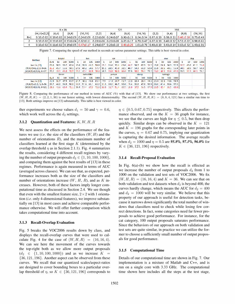
Figure 7. Comparing the speed of our method in seconds at various parameter settings. This table is best viewed in color.

Figure 8. Comparing the performance of our method in terms of AUC (%) with that of [13]. We show our performance at two settings, the first(W,H,R,K) = (2, 2, 1, 36) is our fastest setting, with lowest dimensionality. The second (W,H,R,K) = (8, 8, 4, 121) has a similar run time to[13]. Both settings improve on [13] substantially. This table is best viewed in color.

ther experiments we choose values d1 = 50 and γ = 0.6,which work well across the d2 settings.

3.1.2 Quantization and Features: K,W,H,R

We next assess the effects on the performance of the fea-tures we use (i.e. the size of the classifiers (W,H) and thenumber of orientations R), and the maximum number ofclassifiers learned at the first stage K (determined by theoverlap threshold η as in Section 2.1.1). Fig. 4 summarizesthe results, considering 4 different recall regimes by vary-ing the number of output proposals d2 ∈ {1, 10, 100, 1000},and comparing them against the best results of [13] in theseregimes. Performance is again measured in terms of AUC(averaged across classes). We can see that, as expected, per-formance increases both as the size of the classifiers andnumber of orientations increase (W , H , R), and as K in-creases. However, both of these factors imply longer com-putational time as discussed in Section 2.4. We see thoughthat even with the smallest feature size, 2×2 with 1 orienta-tion (i.e. only 4-dimensional features), we improve substan-tially on [13] in most cases and achieve comparable perfor-mance otherwise. We will offer further comparison whichtakes computational time into account.

3.1.3 Recall-Overlap Evaluation

Fig. 5 breaks the VOC2006 results down by class, anddisplays the recall-overlap curves that were used to cal-culate Fig. 4 for the case of (W,H,R) = (16, 16, 4).We can see here the movement of the curves towardsthe top-right both as we allow more output proposals(d2 ∈ {1, 10, 100, 1000}) and as we increase K ={36, 121, 196}. Another aspect can be observed from thesecurves. We recall that our quantized scales/aspect-ratiosare designed to cover bounding boxes to a particular over-lap threshold of η, so K ∈ {36, 121, 196} corresponds to

η ∈ {0.5, 0.67, 0.75} respectively. This affects the perfor-mance observed, and on the K = 36 graph for instance,we see that the curves are high for η ≤ 0.5, but then dropquickly. Similar drops can be observed in the K = 121and K = 196 graphs for the corresponding later points inthe curves, η = 0.67 and 0.75, implying our quantizationis capturing the desired information. The average recallswhen d2 = 1000 and η = 0.5 are 95.8%, 97.1%, 96.0% forK ∈ {36, 121, 196} respectively.

3.1.4 Recall-Proposal Evaluation

In Fig. 6(a)-(b) we show how the recall is effected aswe increase the number of output proposals d2 from 1 to1000 on the validation and test sets of VOC2006. We fix(W,H,R) = (16, 16, 4) and K = 36. We can see that onboth validation and test datasets when d2 is beyond 400, thecurves hardly change, which means the AUC for d2 = 400and d2 = 1000 will be very similar. We believe that thisproperty of our approach is useful for detection tasks, be-cause it narrows down significantly the total number of win-dows that classifiers need to check while losing few cor-rect detections. In fact, some categories need far fewer pro-posals to achieve good performance. For instance, for thecat category, 100 output proposals saturates performance.Since the behaviors of our approach on both validation andtest sets are quite similar, in practice we can utilize the for-mer to choose a sufficiently small number of output propos-als for good performance.

3.1.5 Computational Time

Details of our computational time are shown in Fig. 7. Ourimplementation is a mixture of Matlab and C++, and isrun on a single core with 3.33 GHz. The computationaltime shown here includes all the steps at the test stage,

1502

Figure 9. Comparing the performance of our method in terms of AUC (%) when no scale/aspect-ratio information is included during learning the classifiers(i.e. single classifier), when only aspect ratio information is included, and when both scale and aspect ratio are included. This table is best viewed in color.

Figure 10. Recall-overlap evaluation for VOC2010. Recall-overlap curves are plotted for individual classes using d2 ∈ {1, 10, 100, 1000} from left toright, andK ∈ {36, 121, 196} from top to bottom. All curves are plotted using (W,H,R) = (16, 16, 4). The numbers shown in the legends are the recallpercentages when the overlap threshold η is set to 0.5. This figure is best viewed in color.

i.e. calculating features, 2D convolution, proposal selec-tion, and ranking score calibration. As we see, with in-crease in the size of the feature windows (W,H), the num-ber of orientation channels R, and the maximum numberof classifiers learned at the first stage K, computationaltime grows roughly linearly in the log-scale. This demon-

strates that the computational complexity of our approachcan be approximated by the complexity of 2D convolution.Moreover, we can compare our time with the 0.47 ± 0.01in [13]1 (based on a 2.8 GHz PC). As mentioned, we already

1In [13], the computational time is only for training models withoutconsidering the time for feature extraction.

1503

substantially outperform this method at our fastest setting,(W,H,R) = (2, 2, 1) and K = 36. In Fig. 7 we highlightthe closest settings of our method to the speed of [13]. Wecan see on Fig. 4 that these all offer further substantial im-provements, and we make a closer comparison in Fig. 8 bycomparing AUC values of [13] with our results at (a) ourfastest setting, and (b) the best of our settings with simi-lar computational time. Averaging across the four outputsettings (d2 ∈ {1, 10, 100, 1000}), [13] achieves 39.9%,while we achieve 44.5% at (W,H,R,K) = (2, 2, 1, 36),and 50.8% at (W,H,R,K) = (8, 8, 4, 121). Our approachis thus quicker, and offers a substantial improvement in out-put quality to [13].

3.1.6 Contribution of Scale and Aspect Ratio

To verify that our two-stage ranking cascade, involving sep-arate ranking of scales and aspect ratios followed by a cali-bration, is contributing to our performance, we give furtherresults in Fig. 9 where during learning the individual clas-sifiers we compare our full system against restricted caseswhere we (a) use only one quantization level, and so do notuse scale and aspect ratio information (thus learning onlyone classifier), and (b) use only aspect ratio information(learning one classifier per aspect ratio). In each case, thefeature size is set to (W,H,R) = (16, 16, 4) and K = 36.As shown, we have an average gain in performance as scaleand aspect ratio information is added (although in certainclasses the effect is less pronounced, and aspect ratio playsa more important role than scale in some).

3.2. VOC2010

We repeat our recall-overlap and recall-proposal eval-uations on VOC2010. In Fig. 6(c) we see a similar pat-tern across classes to the VOC2006 validation and test sets,implying that thresholds can be generalized (even for in-dividual classes) across these datasets. In Fig. 10 we seea similar pattern of results to Fig. 5 (also using the set-ting (W,H,R) = (16, 16, 4)). The average recalls whend2 = 1000 and η = 0.5 are 86.2%, 92.7%, 91.0% forK ∈ {36, 121, 196} respectively, which are comparable tothose in Section 3.1.3. We therefore believe that our ap-proach is robust and efficient across datasets.

4. Conclusion

We have introduced a two-stage cascaded model using aranking SVM framework to generate object detection pro-posals, which we envisage can be used as the initial stagesof a complete object detection pipeline. Our framework nat-urally incorporates scale and aspect ratio information aboutobjects, which are treated separately in the first stage of thecascade, and we emphasize the flexibility of the framework,

where different types of features could easily be incorpo-rated at this stage. Our method is both fast and efficient,and we have shown a substantial improvement in speed andrecall over a state-of-the-art method [13], which also usesa cascade design. Remaining problems for investigation in-clude how to embed our ranking formulation into a globalcost function for a complete detection cascade.

Acknowledgements. We thank P. Sturgess, S. Senguptaand L. Ladicky for useful discussion in this paper. Thiswork was supported by the IST Programme of the Euro-pean Community, under the PASCAL2 Network of Excel-lence, IST-2007-216886. P. H. S. Torr is in receipt of RoyalSociety Wolfson Research Merit Award.

References[1] M. Blaschko and C. Lampert. Learning to localize objects with struc-

tured output regression. In ECCV’08, pages I: 2–15, 2008.[2] M. B. Blaschko, A. Vedaldi, and A. Zisserman. Simultaneous object

detection and ranking with weak supervision. In NIPS’10, 2010.[3] S. Bucak, P. Mallapragada, R. Jin, and A. Jain. Efficient multi-label

ranking for multi-class learning: Application to object recognition.In ICCV’09, pages 2098–2105, 2009.

[4] O. Chum and A. Zisserman. An exemplar model for learning objectclasses. In CVPR’07, pages 1–8, 2007.

[5] N. Dalal and B. Triggs. Histograms of oriented gradients for humandetection. In CVPR’05, pages I: 886–893, 2005.

[6] M. Everingham, L. Van Gool, C. K. I. Williams, J. Winn,and A. Zisserman. The PASCAL Visual Object ClassesChallenge 2010 (VOC2010) Results. http://www.pascal-network.org/challenges/VOC/voc2010/workshop/index.html.

[7] M. Everingham, A. Zisserman, C. K. I. Williams, andL. Van Gool. The PASCAL Visual Object ClassesChallenge 2006 (VOC2006) Results. http://www.pascal-network.org/challenges/VOC/voc2006/results.pdf.

[8] P. Felzenszwalb, R. Girshick, and D. McAllester. Cascade objectdetection with deformable part models. In CVPR’10, pages 2241–2248, 2010.

[9] P. Felzenszwalb, R. Girshick, D. McAllester, and D. Ramanan. Ob-ject detection with discriminatively trained part-based models. PAMI,32(9):1627–1645, September 2010.

[10] P. Gehler and S. Nowozin. On feature combination for multiclassobject classification. In ICCV’09, pages 221–228, 2009.

[11] J. Gonfaus, X. Boix, J. van de Weijer, A. Bagdanov, J. Serrat, andJ. Gonzalez. Harmony potentials for joint classification and segmen-tation. In CVPR’10, pages 3280–3287, 2010.

[12] R. Herbrich, T. Graepel, and K. Obermayer. Large margin rankboundaries for ordinal regression. In Advances in Large MarginClassifiers, pages 115–132, 2000.

[13] C. Lampert. An efficient divide-and-conquer cascade for nonlinearobject detection. In CVPR’10, pages 1022–1029, 2010.

[14] C. Lampert, M. Blaschko, and T. Hofmann. Efficient subwindowsearch: A branch and bound framework for object localization.PAMI, 31(12):2129–2142, December 2009.

[15] F. Li, J. Carreira, and C. Sminchisescu. Object recognition as rankingholistic figure-ground hypotheses. In CVPR’10, pages 1712–1719,2010.

[16] D. Park, D. Ramanan, and C. Fowlkes. Multiresolution models forobject detection. In ECCV’10, pages 241–254, 2010.

[17] A. Vedaldi, V. Gulshan, M. Varma, and A. Zisserman. Multiple ker-nels for object detection. In ICCV’09, 2009.

1504