Proposal Flow

Bumsub Ham1,∗ ,† Minsu Cho1,∗ ,† Cordelia Schmid1,‡ Jean Ponce2,†

1Inria 2Ecole Normale Superieure / PSL Research University

AbstractFinding image correspondences remains a challenging

problem in the presence of intra-class variations and large

changes in scene layout. Semantic flow methods are de-

signed to handle images depicting different instances of the

same object or scene category. We introduce a novel ap-

proach to semantic flow, dubbed proposal flow, that estab-

lishes reliable correspondences using object proposals. Un-

like prevailing semantic flow approaches that operate on

pixels or regularly sampled local regions, proposal flow

benefits from the characteristics of modern object propos-

als, that exhibit high repeatability at multiple scales, and

can take advantage of both local and geometric consis-

tency constraints among proposals. We also show that pro-

posal flow can effectively be transformed into a conven-

tional dense flow field. We introduce a new dataset that can

be used to evaluate both general semantic flow techniques

and region-based approaches such as proposal flow. We use

this benchmark to compare different matching algorithms,

object proposals, and region features within proposal flow,

to the state of the art in semantic flow. This comparison,

along with experiments on standard datasets, demonstrates

that proposal flow significantly outperforms existing seman-

tic flow methods in various settings.

1. IntroductionClassical approaches to finding correspondences across

images are designed to handle scenes that contain the same

objects with moderate view point variations in applications

such as stereo matching [42, 47], optical flow [23, 46, 52],

and wide-baseline matching [41, 54]. Semantic flow meth-

ods, such as SIFT Flow [35] for example, on the other

hand, are designed to handle a much higher degree of vari-

ability in appearance and scene layout, typical of images

depicting different instances of the same object or scene

category. They have proven useful for many tasks such as

scene recognition, image registration, semantic segmenta-

tion, and image editing and synthesis [20, 29, 35, 54, 57].

∗indicates equal contribution†WILLOW project-team, Departement d’Informatique de l’Ecole Nor-

male Superieure, ENS/Inria/CNRS UMR 8548.‡Thoth project-team, Inria Grenoble Rhone-Alpes, Laboratoire Jean

Kuntzmann.

0

20

40

60

80

100

120

140

160

(a) Region-based semantic flow. (b) Dense flow field.

Figure 1. Proposal flow generates a reliable semantic flow between

similar images using local and geometric consistency constraints

among object proposals, and it can be transformed into a dense

flow field. (a) Region-based semantic flow. (b) Dense flow field

and image warping using the flow field. (Best viewed in color.)

In this context, however, appearance and shape variations

may confuse similarity measures for local region matching,

and prohibit the use of strong geometric constraints (e.g.,

epipolar geometry, limited disparity range). Existing ap-

proaches to semantic flow are thus easily distracted by scene

elements specific to individual objects and image-specific

details (e.g., background, texture, occlusion, clutter). This

is the motivation for our work, where we use robust region

correspondences to focus on regions containing prominent

objects and scene elements rather than clutter and distract-

ing details.

Concretely, we introduce an approach to semantic flow

computation, called proposal flow, that establishes region

correspondences using object proposals and their geomet-

ric relations (Fig. 1). Unlike previous semantic flow al-

gorithms [4, 20, 22, 25, 29, 35, 45, 49, 50, 54, 57], that

use regular grid structures for local region generation and

matching, we leverage a large number of multi-scale object

proposals [1, 24, 40, 51, 58], as now widely used in object

detection [19, 27]. The proposed approach establishes re-

gion correspondences by exploiting their visual features and

geometric relations in an efficient manner, and generates

a region-based semantic flow composed of object proposal

matches. We also show that the proposal flow can be effec-

tively transformed into a conventional dense flow field. Fi-

nally, we introduce a new dataset that can be used to evalu-

3475

ate both general semantic flow techniques and region-based

approaches such as proposal flow. We use this benchmark

to compare different matching algorithms, object proposals,

and region features within proposal flow, to the state of the

art in semantic flow. This comparison, along with experi-

ments on standard datasets, demonstrates that proposal flow

significantly outperforms existing semantic flow methods in

various settings.

2. Related workCorrespondence problems involve a broad range of top-

ics beyond the scope of this paper. Here we briefly de-

scribe the context of our approach, and only review repre-

sentative works pertinent for ours. Classical approaches to

stereo matching and optical flow estimate pixel-level dense

correspondences between two nearby images of the same

scene [23, 41, 42]. While advances in invariant feature de-

tection and description have revolutionized object recog-

nition and reconstruction in the past 15 years, research

on image matching and alignment between images have

long been dominated by instance matching with the same

scene and objects [18]. Unlike these, several recent ap-

proaches to semantic flow focus on handling images con-

taining different scenes and objects. Graph-based match-

ing algorithms [10, 14] attempt to find category-level fea-

ture matches by leveraging a flexible graph representation

of images, but they commonly handle sparsely sampled or

detected features due to their computational complexity. In-

spired by classic optical flow algorithms, Liu et al. pio-

neered the idea of dense correspondences across different

scenes, and proposed the SIFT Flow [35] algorithm that

uses a multi-resolution image pyramid together with a hi-

erarchical optimization technique for efficiency. Kim et

al. [29] extended the approach by inducing a multi-scale

regularization with a hierarchically connected pyramid of

grid graphs. More recently, Long et al. [36] have investi-

gated the effect of pretrained ConvNet features on the SIFT

Flow algorithm, and Bristow et al. [4] have proposed an

exemplar-LDA approach that improves the performance of

semantic flow. Despite differences in graph construction,

optimization, and similarity computation, existing seman-

tic flow approaches share grid-based regular sampling and

spatial regularization: The appearance similarity is defined

at each region or pixel on (a pyramid of) regular grids, and

spatial regularization is imposed between neighboring re-

gions in the pyramid models [29, 35]. In contrast, our work

builds on generic object proposals with diverse spatial sup-

ports [1, 24, 40, 51, 58], and uses an irregular form of spatial

regularization based on co-occurrence and overlap of the

proposals. We show that the use of local regularization with

object proposals yields substantial gains in generic region

matching and semantic flow, in particular when handling

images with significant clutter and intra-class variations.

Object proposals [1, 24, 40, 51, 58] have originally been

developed for object detection, where they are used to re-

duce the search space as well as false alarms. They are now

an important component in many state-of-the-art detection

pipelines [19, 27]. Despite their success on object detection

and segmentation, they have seldom been used in matching

tasks [9, 26]. In particular, while Cho et al. [9] have shown

that object proposals are useful for region matching due to

their high repeatability on salient part regions, the use of

object proposals has never been thoroughly investigated in

semantic flow computation. The approach proposed in this

paper is a first step in this direction, and we explore how the

choice of object proposals, matching algorithms, and fea-

tures affects matching robustness and accuracy.

Contributions. The contributions of this paper are three-

fold: (i) We introduce the proposal flow approach to es-

tablishing robust region correspondences between related,

but not identical scenes using object proposals. (ii) We in-

troduce a benchmark for semantic flow that can be used to

evaluate both general semantic flow algorithms and region

matching methods. (iii) We demonstrate the advantage of

proposal flow over state-of-the-art semantic flow methods

through extensive experimental evaluations.

3. Proposal flowProposal flow can use any type of object proposals [1, 24,

40, 51, 58] as candidate regions for matching two images of

related scenes. In this section, we introduce a probabilis-

tic model for region matching, and describe three matching

strategies including two baselines and a new one using local

regularization. We then describe our approach to generating

a dense flow field from the region matches.

3.1. A Bayesian model for region matching

Let us suppose that two sets of object proposals R and

R0 have been extracted from images I and I 0 (Fig. 2(a-b)).

A proposal r in R is an image region r = (f, s) with ap-

pearance feature f and spatial support s. The appearance

feature represents a visual descriptor for the region (e.g.,

SPM [31] , HOG [11], ConvNet [30]), and the spatial sup-

port describes the set of all pixel positions in the region,

that forms a rectangular box in this work. Given the data

D = (R,R0), we wish to estimate a posterior probability

of the event r 7! r0 meaning that proposal r in R matches

proposal r0 in R0:

p(r 7! r0 | D) = p(f 7! f 0)p(s 7! s0 | D), (1)

where we decouple the probabilities of appearance and spa-

tial support matching, and assume that appearance match-

ing is independent of D. In practice, the appearance term

p(f 7! f 0) is simply computed from a similarity between

feature descriptors f and f 0, and the geometric consistency

term p(s 7! s0 | D) is evaluated by comparing the spatial

supports s and s0 in the context of the given data D, as de-

scribed in the next section. We set the posterior probability

3476

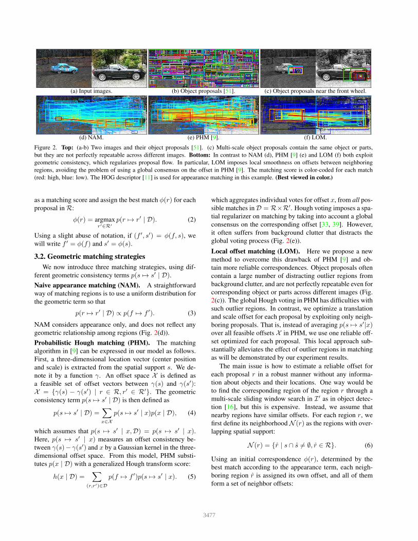
(a) Input images. (b) Object proposals [51]. (c) Object proposals near the front wheel.

(d) NAM. (e) PHM [9]. (f) LOM.

Figure 2. Top: (a-b) Two images and their object proposals [51]. (c) Multi-scale object proposals contain the same object or parts,

but they are not perfectly repeatable across different images. Bottom: In contrast to NAM (d), PHM [9] (e) and LOM (f) both exploit

geometric consistency, which regularizes proposal flow. In particular, LOM imposes local smoothness on offsets between neighboring

regions, avoiding the problem of using a global consensus on the offset in PHM [9]. The matching score is color-coded for each match

(red: high, blue: low). The HOG descriptor [11] is used for appearance matching in this example. (Best viewed in color.)

as a matching score and assign the best match φ(r) for each

proposal in R:

φ(r) = argmaxr02R0

p(r 7! r0 | D). (2)

Using a slight abuse of notation, if (f 0, s0) = φ(f, s), we

will write f 0 = φ(f) and s0 = φ(s).

3.2. Geometric matching strategies

We now introduce three matching strategies, using dif-

ferent geometric consistency terms p(s 7! s0 | D).

Naive appearance matching (NAM). A straightforward

way of matching regions is to use a uniform distribution for

the geometric term so that

p(r 7! r0 | D) / p(f 7! f 0). (3)

NAM considers appearance only, and does not reflect any

geometric relationship among regions (Fig. 2(d)).

Probabilistic Hough matching (PHM). The matching

algorithm in [9] can be expressed in our model as follows.

First, a three-dimensional location vector (center position

and scale) is extracted from the spatial support s. We de-

note it by a function γ. An offset space X is defined as

a feasible set of offset vectors between γ(s) and γ(s0):X = {γ(s) − γ(s0) | r 2 R, r0 2 R0}. The geometric

consistency term p(s 7! s0 | D) is then defined as

p(s 7! s0 | D) =X

x2X

p(s 7! s0 | x)p(x | D), (4)

which assumes that p(s 7! s0 | x,D) = p(s 7! s0 | x).Here, p(s 7! s0 | x) measures an offset consistency be-

tween γ(s)− γ(s0) and x by a Gaussian kernel in the three-

dimensional offset space. From this model, PHM substi-

tutes p(x | D) with a generalized Hough transform score:

h(x | D) =X

(r,r0)2D

p(f 7! f 0)p(s 7! s0 | x). (5)

which aggregates individual votes for offset x, from all pos-

sible matches in D = R⇥R0. Hough voting imposes a spa-

tial regularizer on matching by taking into account a global

consensus on the corresponding offset [33, 39]. However,

it often suffers from background clutter that distracts the

global voting process (Fig. 2(e)).

Local offset matching (LOM). Here we propose a new

method to overcome this drawback of PHM [9] and ob-

tain more reliable correspondences. Object proposals often

contain a large number of distracting outlier regions from

background clutter, and are not perfectly repeatable even for

corresponding object or parts across different images (Fig.

2(c)). The global Hough voting in PHM has difficulties with

such outlier regions. In contrast, we optimize a translation

and scale offset for each proposal by exploiting only neigh-

boring proposals. That is, instead of averaging p(s 7! s0|x)over all feasible offsets X in PHM, we use one reliable off-

set optimized for each proposal. This local approach sub-

stantially alleviates the effect of outlier regions in matching

as will be demonstrated by our experiment results.

The main issue is how to estimate a reliable offset for

each proposal r in a robust manner without any informa-

tion about objects and their locations. One way would be

to find the corresponding region of the region r through a

multi-scale sliding window search in I 0 as in object detec-

tion [16], but this is expensive. Instead, we assume that

nearby regions have similar offsets. For each region r, we

first define its neighborhood N (r) as the regions with over-

lapping spatial support:

N (r) = {r | s \ s 6= ;, r 2 R}. (6)

Using an initial correspondence φ(r), determined by the

best match according to the appearance term, each neigh-

boring region r is assigned its own offset, and all of them

form a set of neighbor offsets:

3477

X (r) = {γ(s)− γ(φ(s)) | r 2 N (r)}. (7)

From this set of neighbor offsets, we estimate a local offset

x⇤r for the region r by the geometric median [37]1:

x⇤r = argmin

x2R3

X

y2X (r)

kx− yk2 , (8)

which can be globally optimized by Weiszfeld’s algo-

rithm [6] using a form of iteratively re-weighted least

squares. Based on the local offset x⇤r optimized for each

region, we define the geometric consistency function:

g(s 7! s0|D) = p(s 7! s0|x⇤r)

X

r2N (r)

p(f 7! φ(f)), (9)

which means that r in R is likely to match with r0 in R0 if

their offset is close to the local offset x⇤r , and r has many

neighboring matches with a high appearance fidelity.

By using g(s 7! s0|D) as a proxy for p(s 7! s0|D),LOM imposes local smoothness on offsets between neigh-

boring regions. This geometric consistency function effec-

tively suppresses matches between clutter regions, while fa-

voring matches between regions that contain objects rather

than object parts (Fig. 2(f)). In particular, the use of lo-

cal offsets optimized for each proposal regularizes offsets

within a local neighborhood that incorporates an overlap re-

lationship between spatial supports of regions. This local

regularization avoids a common problem with PHM, where

the matching results often depend on a few strong matches.

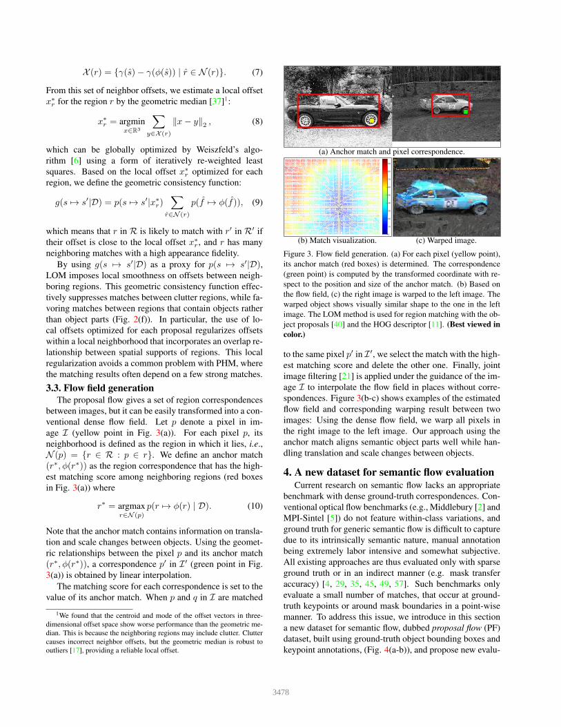
3.3. Flow field generation

The proposal flow gives a set of region correspondences

between images, but it can be easily transformed into a con-

ventional dense flow field. Let p denote a pixel in im-

age I (yellow point in Fig. 3(a)). For each pixel p, its

neighborhood is defined as the region in which it lies, i.e.,

N (p) = {r 2 R : p 2 r}. We define an anchor match

(r⇤, φ(r⇤)) as the region correspondence that has the high-

est matching score among neighboring regions (red boxes

in Fig. 3(a)) where

r⇤ = argmaxr2N (p)

p(r 7! φ(r) | D). (10)

Note that the anchor match contains information on transla-

tion and scale changes between objects. Using the geomet-

ric relationships between the pixel p and its anchor match

(r⇤, φ(r⇤)), a correspondence p0 in I 0 (green point in Fig.

3(a)) is obtained by linear interpolation.

The matching score for each correspondence is set to the

value of its anchor match. When p and q in I are matched

1We found that the centroid and mode of the offset vectors in three-

dimensional offset space show worse performance than the geometric me-

dian. This is because the neighboring regions may include clutter. Clutter

causes incorrect neighbor offsets, but the geometric median is robust to

outliers [17], providing a reliable local offset.

(a) Anchor match and pixel correspondence.

0

10

20

30

40

50

60

70

80

90

(b) Match visualization. (c) Warped image.

Figure 3. Flow field generation. (a) For each pixel (yellow point),

its anchor match (red boxes) is determined. The correspondence

(green point) is computed by the transformed coordinate with re-

spect to the position and size of the anchor match. (b) Based on

the flow field, (c) the right image is warped to the left image. The

warped object shows visually similar shape to the one in the left

image. The LOM method is used for region matching with the ob-

ject proposals [40] and the HOG descriptor [11]. (Best viewed in

color.)

to the same pixel p0 in I 0, we select the match with the high-

est matching score and delete the other one. Finally, joint

image filtering [21] is applied under the guidance of the im-

age I to interpolate the flow field in places without corre-

spondences. Figure 3(b-c) shows examples of the estimated

flow field and corresponding warping result between two

images: Using the dense flow field, we warp all pixels in

the right image to the left image. Our approach using the

anchor match aligns semantic object parts well while han-

dling translation and scale changes between objects.

4. A new dataset for semantic flow evaluationCurrent research on semantic flow lacks an appropriate

benchmark with dense ground-truth correspondences. Con-

ventional optical flow benchmarks (e.g., Middlebury [2] and

MPI-Sintel [5]) do not feature within-class variations, and

ground truth for generic semantic flow is difficult to capture

due to its intrinsically semantic nature, manual annotation

being extremely labor intensive and somewhat subjective.

All existing approaches are thus evaluated only with sparse

ground truth or in an indirect manner (e.g. mask transfer

accuracy) [4, 29, 35, 45, 49, 57]. Such benchmarks only

evaluate a small number of matches, that occur at ground-

truth keypoints or around mask boundaries in a point-wise

manner. To address this issue, we introduce in this section

a new dataset for semantic flow, dubbed proposal flow (PF)

dataset, built using ground-truth object bounding boxes and

keypoint annotations, (Fig. 4(a-b)), and propose new evalu-

3478

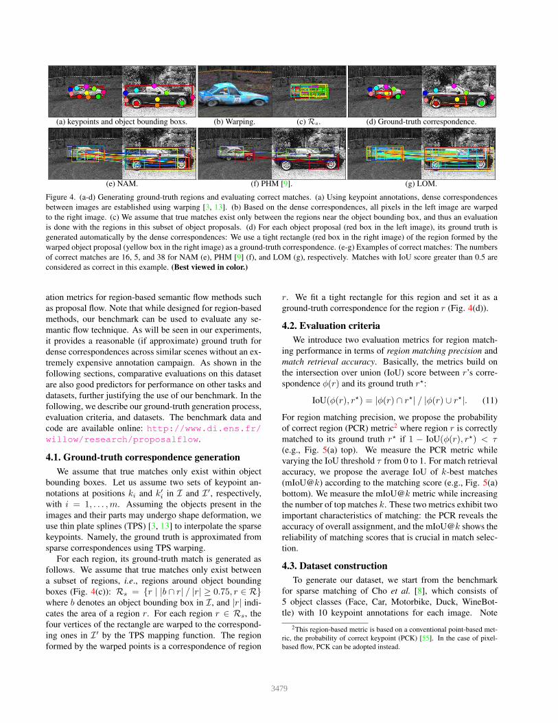
(a) keypoints and object bounding boxs. (b) Warping. (c) Rs. (d) Ground-truth correspondence.

(e) NAM. (f) PHM [9]. (g) LOM.

Figure 4. (a-d) Generating ground-truth regions and evaluating correct matches. (a) Using keypoint annotations, dense correspondences

between images are established using warping [3, 13]. (b) Based on the dense correspondences, all pixels in the left image are warped

to the right image. (c) We assume that true matches exist only between the regions near the object bounding box, and thus an evaluation

is done with the regions in this subset of object proposals. (d) For each object proposal (red box in the left image), its ground truth is

generated automatically by the dense correspondences: We use a tight rectangle (red box in the right image) of the region formed by the

warped object proposal (yellow box in the right image) as a ground-truth correspondence. (e-g) Examples of correct matches: The numbers

of correct matches are 16, 5, and 38 for NAM (e), PHM [9] (f), and LOM (g), respectively. Matches with IoU score greater than 0.5 are

considered as correct in this example. (Best viewed in color.)

ation metrics for region-based semantic flow methods such

as proposal flow. Note that while designed for region-based

methods, our benchmark can be used to evaluate any se-

mantic flow technique. As will be seen in our experiments,

it provides a reasonable (if approximate) ground truth for

dense correspondences across similar scenes without an ex-

tremely expensive annotation campaign. As shown in the

following sections, comparative evaluations on this dataset

are also good predictors for performance on other tasks and

datasets, further justifying the use of our benchmark. In the

following, we describe our ground-truth generation process,

evaluation criteria, and datasets. The benchmark data and

code are available online: http://www.di.ens.fr/

willow/research/proposalflow.

4.1. Ground-truth correspondence generation

We assume that true matches only exist within object

bounding boxes. Let us assume two sets of keypoint an-

notations at positions ki and k0i in I and I 0, respectively,

with i = 1, . . . ,m. Assuming the objects present in the

images and their parts may undergo shape deformation, we

use thin plate splines (TPS) [3, 13] to interpolate the sparse

keypoints. Namely, the ground truth is approximated from

sparse correspondences using TPS warping.

For each region, its ground-truth match is generated as

follows. We assume that true matches only exist between

a subset of regions, i.e., regions around object bounding

boxes (Fig. 4(c)): Rs = {r | |b \ r| / |r| ≥ 0.75, r 2 R}where b denotes an object bounding box in I, and |r| indi-

cates the area of a region r. For each region r 2 Rs, the

four vertices of the rectangle are warped to the correspond-

ing ones in I 0 by the TPS mapping function. The region

formed by the warped points is a correspondence of region

r. We fit a tight rectangle for this region and set it as a

ground-truth correspondence for the region r (Fig. 4(d)).

4.2. Evaluation criteria

We introduce two evaluation metrics for region match-

ing performance in terms of region matching precision and

match retrieval accuracy. Basically, the metrics build on

the intersection over union (IoU) score between r’s corre-

spondence φ(r) and its ground truth r?:

IoU(φ(r), r?) = |φ(r) \ r?| / |φ(r) [ r?|. (11)

For region matching precision, we propose the probability

of correct region (PCR) metric2 where region r is correctly

matched to its ground truth r? if 1 − IoU(φ(r), r?) < τ(e.g., Fig. 5(a) top). We measure the PCR metric while

varying the IoU threshold τ from 0 to 1. For match retrieval

accuracy, we propose the average IoU of k-best matches

(mIoU@k) according to the matching score (e.g., Fig. 5(a)

bottom). We measure the mIoU@k metric while increasing

the number of top matches k. These two metrics exhibit two

important characteristics of matching: the PCR reveals the

accuracy of overall assignment, and the mIoU@k shows the

reliability of matching scores that is crucial in match selec-

tion.

4.3. Dataset construction

To generate our dataset, we start from the benchmark

for sparse matching of Cho et al. [8], which consists of

5 object classes (Face, Car, Motorbike, Duck, WineBot-

tle) with 10 keypoint annotations for each image. Note

2This region-based metric is based on a conventional point-based met-

ric, the probability of correct keypoint (PCK) [55]. In the case of pixel-

based flow, PCK can be adopted instead.

3479

that these images contain more clutter and intra-class vari-

ation than existing datasets for semantic flow evaluation,

e.g., images with tightly cropped objects or similar back-

ground [29, 45, 57]. We exclude the Face class where the

number of generated object proposals is not sufficient to

evaluate matching accuracy. The other classes are split into

sub-classes3 according to viewpoint or background clutter.

We obtain a total of 10 sub-classes. Given these images and

regions, we generate ground-truth data between all possible

image pairs within each class.

5. Experiments

5.1. Experimental details

Object proposals. We evaluate four state-of-the-art

object proposal methods: EdgeBox (EB) [58], multi-

scale combinatorial grouping (MCG) [1], selective

search (SS) [51], and randomized prim (RP) [40]. In addi-

tion, we consider three baseline proposals [24]: Uniform

sampling (US), Gaussian sampling (GS), and sliding win-

dow (SW). See [24] for more details. For fair comparison,

we use 1,000 proposals for all the methods. To control the

number of proposals, we use the proposal score provided

by EB, MCG, and SS. For RP, we randomly select among

the proposals.

Feature descriptors and similarity. We evaluate three

popular feature descriptors: SPM [31], HOG [11], and Con-

vNet [30]. For SPM, dense SIFT features [38] are extracted

every 4 pixels and each descriptor is quantized into a 1,000

word codebook [48]. For each region, a spatial pyramid

pooling [31] is used with 1⇥1 and 3⇥3 pooling regions. We

compute the similarity between SPM descriptors by the χ2

kernel. HOG features are extracted with 8 ⇥ 8 cells and 31

orientations, then whitened. For ConvNet features, we use

each output of the 5 convolutional layers in AlexNet [30],

which is pre-trained on the ImageNet dataset [12]. For HOG

and ConvNet, the dot product is used as a similarity metric.

5.2. Proposal flow components

We use the PF benchmark in this section to compare

three variants of proposal flow using different matching al-

gorithms (NAM, PHM, LOM), combined with various ob-

ject proposals [1, 24, 40, 51, 58], and features [11, 30, 31].

Figure 4(e-g) shows a qualitative comparison between

region matching algorithms on a pair of images and depicts

correct matches found by each variant of proposal flow. In

this example, at the IoU threshold 0.5, the numbers of cor-

rect matches are 16, 5, and 38 for NAM, PHM [9], and

3They are car (S), (G), (M), duck (S), motorbike (S), (G), (M), wine

bottle (w/o C), (w/ C), (M), where (S) and (G) denote side and general

viewpoints, respectively. (C) stands for background clutter, and (M) de-

notes mixed viewpoints (side + general) for car and motorbike classes and

a combination of images in wine bottle (w/o C + w/ C) for the wine bottle

class. The dataset has 10 images for each class, thus 100 images in total.

LOM, respectively. This shows that PHM may give worse

performance than even NAM when much clutter exists in

background. In contrast, the local regularization in LOM

alleviates the effect of such clutter.

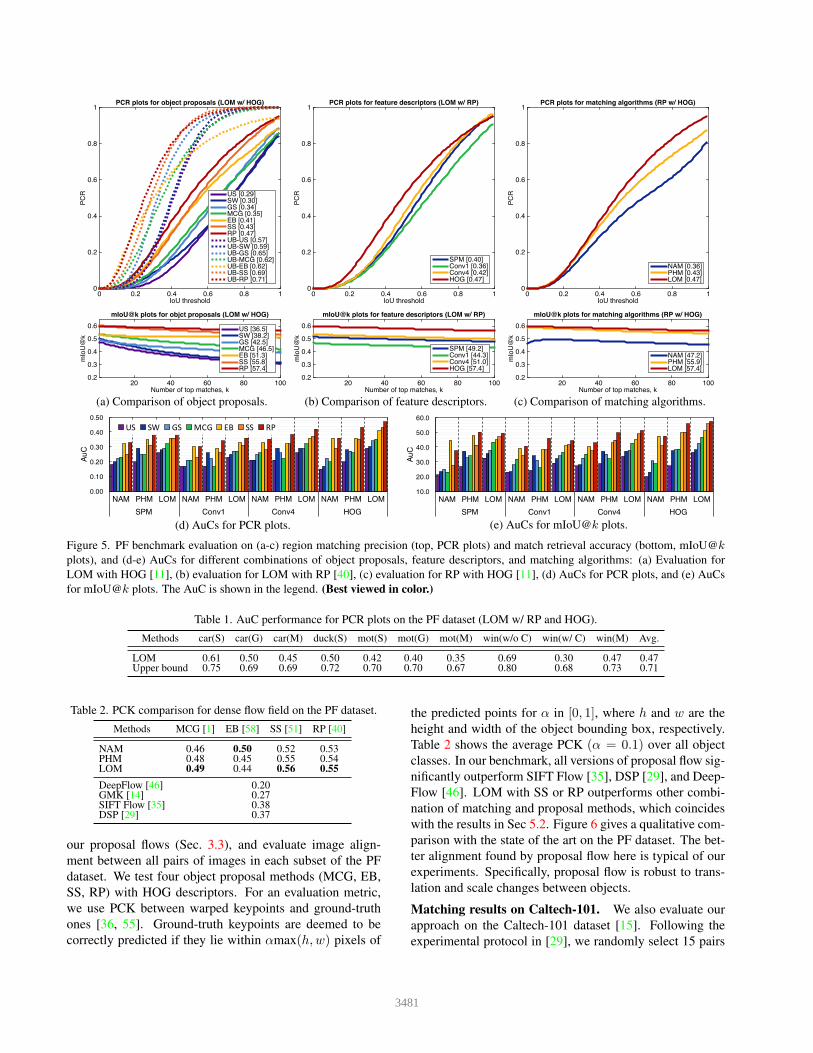
Figure 5 summarizes the matching and retrieval perfor-

mance on average for all object classes with a variety of

combination of object proposals, feature descriptors, and

matching algorithms. Figure 5(a) compares different types

of object proposals with fixed matching algorithm and fea-

ture descriptor (LOM w/ HOG). RP shows the best match-

ing precision and retrieval accuracy among the object pro-

posals. An upper bound on precision is measured for ob-

ject proposals (around a given object) in the image I us-

ing a corresponding ground truths in image I 0, that is the

best matching accuracy we can achieve with each proposal

method. The upper bound (UB) plots show that RP gen-

erates more consistent regions than other proposal meth-

ods, and is adequate for region matching. RP shows higher

matching precision than other proposals especially when

the IoU threshold is low. The evaluation results for dif-

ferent features (LOM w/ RP) are shown in Fig. 5(b). The

HOG descriptor gives the best performance in matching

and retrieval. The CNN features in our comparison come

from AlexNet [30] trained for ImageNet classification. Such

CNN features have a task-specific bias to capture discrim-

inative parts for classification, which may be less adequate

for patch correspondence or retrieval than engineered fea-

tures such as HOG. Similar conclusions are found in re-

cent papers [36, 43]. See, for example, Table 3 in [43]

where SIFT outperforms all AlexNet features (Conv1-5).

Among ConvNet features, the fourth and first convolutional

layers (Conv4 and Conv1) show the best and worst per-

formance, respectively, while other layers perform similar

to SPM. This confirms the finding in [56], which shows

that Conv4 gives the best matching performance among

ImageNet-trained ConvNet features. Figure 5(c) compares

the performance of different matching algorithms (RP w/

HOG), and shows that LOM outperforms others in match-

ing as well as retrieval. Figure 5(d and e) shows the area un-

der curve (AuC) for PCR and mIoU@k plots, respectively.

This suggests that combining LOM, RP, and HOG performs

best in both metrics.

In Table 1, we show AuCs of PCR plots for each class

(LOM w/ RP and HOG). From this table, we can see

that 1) higher matching precision is achieved with objects

having a similar pose (e.g., mot(S) vs. mot(M)), 2) per-

formance decreases for deformable object matching (e.g.,

duck(S) vs. car(S)), and 3) matching precision can in-

crease drastically by eliminating background clutters (e.g.,

win(w/o C) vs. win(w/ C)).

5.3. Flow field

To compare our method with state-of-the-art seman-

tic flow methods, we compute a dense flow field from

3480

IoU threshold0 0.2 0.4 0.6 0.8 1

PC

R

0

0.2

0.4

0.6

0.8

1PCR plots for object proposals (LOM w/ HOG)

US [0.29]SW [0.30]GS [0.34]MCG [0.35]EB [0.41]SS [0.43]RP [0.47]UB-US [0.57]UB-SW [0.59]UB-GS [0.65]UB-MCG [0.62]UB-EB [0.62]UB-SS [0.69]UB-RP [0.71]

IoU threshold0 0.2 0.4 0.6 0.8 1

PC

R

0

0.2

0.4

0.6

0.8

1PCR plots for feature descriptors (LOM w/ RP)

SPM [0.40]Conv1 [0.36]Conv4 [0.42]HOG [0.47]

IoU threshold0 0.2 0.4 0.6 0.8 1

PC

R

0

0.2

0.4

0.6

0.8

1PCR plots for matching algorithms (RP w/ HOG)

NAM [0.36]PHM [0.43]LOM [0.47]

Number of top matches, k20 40 60 80 100

mIo

U@

k

0.2

0.3

0.4

0.5

0.6

mIoU@k plots for objct proposals (LOM w/ HOG)

US [36.5]SW [38.2]GS [42.5]MCG [46.5]EB [51.3]SS [55.8]RP [57.4]

(a) Comparison of object proposals.Number of top matches, k

20 40 60 80 100

mIo

U@

k

0.2

0.3

0.4

0.5

0.6

mIoU@k plots for feature descriptors (LOM w/ RP)

SPM [49.2]Conv1 [44.3]Conv4 [51.0]HOG [57.4]

(b) Comparison of feature descriptors.Number of top matches, k

20 40 60 80 100

mIo

U@

k

0.2

0.3

0.4

0.5

0.6

mIoU@k plots for matching algorithms (RP w/ HOG)

NAM [47.2]PHM [55.9]LOM [57.4]

(c) Comparison of matching algorithms.

0.00

0.10

0.20

0.30

0.40

0.50

NAM PHM LOM NAM PHM LOM NAM PHM LOM NAM PHM LOM

SPM Conv1 Conv4 HOG

AuC

US SW GS MCG EB SS RP

(d) AuCs for PCR plots.

10.0

20.0

30.0

40.0

50.0

60.0

NAM PHM LOM NAM PHM LOM NAM PHM LOM NAM PHM LOM

SPM Conv1 Conv4 HOG

AuC

(e) AuCs for mIoU@k plots.

Figure 5. PF benchmark evaluation on (a-c) region matching precision (top, PCR plots) and match retrieval accuracy (bottom, mIoU@k

plots), and (d-e) AuCs for different combinations of object proposals, feature descriptors, and matching algorithms: (a) Evaluation for

LOM with HOG [11], (b) evaluation for LOM with RP [40], (c) evaluation for RP with HOG [11], (d) AuCs for PCR plots, and (e) AuCs

for mIoU@k plots. The AuC is shown in the legend. (Best viewed in color.)

Table 1. AuC performance for PCR plots on the PF dataset (LOM w/ RP and HOG).

Methods car(S) car(G) car(M) duck(S) mot(S) mot(G) mot(M) win(w/o C) win(w/ C) win(M) Avg.

LOM 0.61 0.50 0.45 0.50 0.42 0.40 0.35 0.69 0.30 0.47 0.47Upper bound 0.75 0.69 0.69 0.72 0.70 0.70 0.67 0.80 0.68 0.73 0.71

Table 2. PCK comparison for dense flow field on the PF dataset.

Methods MCG [1] EB [58] SS [51] RP [40]

NAM 0.46 0.50 0.52 0.53PHM 0.48 0.45 0.55 0.54LOM 0.49 0.44 0.56 0.55

DeepFlow [46] 0.20GMK [14] 0.27SIFT Flow [35] 0.38DSP [29] 0.37

our proposal flows (Sec. 3.3), and evaluate image align-

ment between all pairs of images in each subset of the PF

dataset. We test four object proposal methods (MCG, EB,

SS, RP) with HOG descriptors. For an evaluation metric,

we use PCK between warped keypoints and ground-truth

ones [36, 55]. Ground-truth keypoints are deemed to be

correctly predicted if they lie within αmax(h,w) pixels of

the predicted points for α in [0, 1], where h and w are the

height and width of the object bounding box, respectively.

Table 2 shows the average PCK (α = 0.1) over all object

classes. In our benchmark, all versions of proposal flow sig-

nificantly outperform SIFT Flow [35], DSP [29], and Deep-

Flow [46]. LOM with SS or RP outperforms other combi-

nation of matching and proposal methods, which coincides

with the results in Sec 5.2. Figure 6 gives a qualitative com-

parison with the state of the art on the PF dataset. The bet-

ter alignment found by proposal flow here is typical of our

experiments. Specifically, proposal flow is robust to trans-

lation and scale changes between objects.

Matching results on Caltech-101. We also evaluate our

approach on the Caltech-101 dataset [15]. Following the

experimental protocol in [29], we randomly select 15 pairs

3481

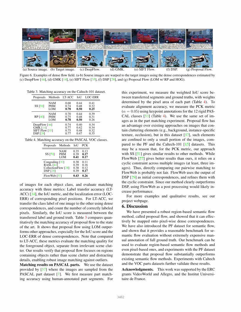
(a) Source image. (b) Target image. (c) DeepFlow. (d) GMK. (e) SIFT Flow. (f) DSP. (g) Proposal Flow.

Figure 6. Examples of dense flow field. (a-b) Sourse images are warped to the target images using the dense correspondences estimated by

(c) DeepFlow [46], (d) GMK [14], (e) SIFT Flow [35], (f) DSP [29], and (g) Proposal Flow (LOM w/ RP and HOG).

Table 3. Matching accuracy on the Caltech-101 dataset.

Proposals Methods LT-ACC IoU LOC-ERR

SS [51]NAM 0.68 0.44 0.41PHM 0.74 0.48 0.32LOM 0.78 0.50 0.25

RP [40]NAM 0.70 0.44 0.39PHM 0.75 0.48 0.31LOM 0.78 0.50 0.26

DeepFlow [46] 0.74 0.40 0.34GMK [14] 0.77 0.42 0.34SIFT Flow [35] 0.75 0.48 0.32DSP [29] 0.77 0.47 0.35

Table 4. Matching accuracy on the PASCAL VOC classes.

Proposals Methods IoU PCK

SS [51]NAM 0.35 0.13PHM 0.39 0.17LOM 0.41 0.17

Congealing [32] 0.38 0.11RASL [44] 0.39 0.16CollectionFlow [28] 0.38 0.12DSP [29] 0.39 0.17

FlowWeb [57] 0.43 0.26

of images for each object class, and evaluate matching

accuracy with three metrics: Label transfer accuracy (LT-

ACC) [34], the IoU metric, and the localization error (LOC-

ERR) of corresponding pixel positions. For LT-ACC, we

transfer the class label of one image to the other using dense

correspondences, and count the number of correctly labeled

pixels. Similarly, the IoU score is measured between the

transferred label and ground truth. Table 3 compares quan-

titatively the matching accuracy of proposal flow to the state

of the art. It shows that proposal flow using LOM outper-

forms other approaches, especially for the IoU score and the

LOC-ERR of dense correspondences. Note that compared

to LT-ACC, these metrics evaluate the matching quality for

the foreground object, separate from irrelevant scene clut-

ter. Our results verify that proposal flow focuses on regions

containing objects rather than scene clutter and distracting

details, enabling robust image matching against outliers.

Matching results on PASCAL parts. We use the dataset

provided by [57] where the images are sampled from the

PASCAL part dataset [7]. We first measure part match-

ing accuracy using human-annotated part segments. For

this experiment, we measure the weighted IoU score be-

tween transferred segments and ground truths, with weights

determined by the pixel area of each part (Table 4). To

evaluate alignment accuracy, we measure the PCK metric

(α = 0.05) using keypoint annotations for the 12 rigid PAS-

CAL classes [53] (Table 4). We use the same set of im-

ages as in the part matching experiment. Proposal flow has

an advantage over existing approaches on images that con-

tain cluttering elements (e.g., background, instance-specific

texture, occlusion), but in this dataset [57], such elements

are confined to only a small portion of the images, com-

pared to the PF and the Caltech-101 [15] datasets. This

may be a reason that, for the PCK metric, our approach

with SS [51] gives similar results to other methods. While

FlowWeb [57] gives better results than ours, it relies on a

cyclic constraint across multiple images (at least, three im-

ages). Thus, directly comparing our pairwise matching to

FlowWeb is probably not fair. FlowWeb uses the output of

DSP [29] as initial correspondences, and refines them with

the cyclic constraint. Since our method clearly outperforms

DSP, using FlowWeb as a post processing would likely in-

crease performance.

For more examples and qualitative results, see our

project webpage.

6. DiscussionWe have presented a robust region-based semantic flow

method, called proposal flow, and showed that it can effec-

tively be mapped onto pixel-wise dense correspondences.

We have also introduced the PF dataset for semantic flow,

and shown that it provides a reasonable benchmark for se-

mantic flow evaluation without extremely expensive man-

ual annotation of full ground truth. Our benchmark can be

used to evaluate region-based semantic flow methods and

even pixel-based ones, and experiments with the PF dataset

demonstrate that proposal flow substantially outperforms

existing semantic flow methods. Experiments with Caltech

and the VOC parts datasets further validate these results.

Acknowledgments. This work was supported by the ERC

grants VideoWorld and Allegro, and the Institut Universi-

taire de France.

3482

References

[1] P. Arbelaez, J. Pont-Tuset, J. Barron, F. Marques, and J. Ma-

lik. Multiscale combinatorial grouping. In CVPR, 2014. 1,

2, 6, 7

[2] S. Baker, D. Scharstein, J. Lewis, S. Roth, M. J. Black, and

R. Szeliski. A database and evaluation methodology for op-

tical flow. IJCV, 92(1):1–31, 2011. 4

[3] F. L. Bookstein. Principal warps: Thin-plate splines and the

decomposition of deformations. IEEE TPAMI, (6):567–585,

1989. 5

[4] H. Bristow, J. Valmadre, and S. Lucey. Dense semantic cor-

respondence where every pixel is a classifier. In ICCV, 2015.

1, 2, 4

[5] D. J. Butler, J. Wulff, G. B. Stanley, and M. J. Black. A

naturalistic open source movie for optical flow evaluation.

In ECCV. 2012. 4

[6] R. Chandrasekaran and A. Tamir. Open questions concerning

weiszfeld’s algorithm for the fermat-weber location problem.

Mathematical Programming, 44(1-3):293–295, 1989. 4

[7] X. Chen, R. Mottaghi, X. Liu, S. Fidler, R. Urtasun, et al.

Detect what you can: Detecting and representing objects us-

ing holistic models and body parts. In CVPR, 2014. 8

[8] M. Cho, K. Alahari, and J. Ponce. Learning graphs to match.

In ICCV, 2013. 5

[9] M. Cho, S. Kwak, C. Schmid, and J. Ponce. Unsupervised

object discovery and localization in the wild: Part-based

matching using bottom-up region proposals. In CVPR, 2015.

2, 3, 5, 6

[10] M. Cho and K. M. Lee. Progressive graph matching: Making

a move of graphs via probabilistic voting. In CVPR. 2

[11] N. Dalal and B. Triggs. Histograms of oriented gradients for

human detection. In CVPR, 2005. 2, 3, 4, 6, 7

[12] J. Deng, W. Dong, R. Socher, L.-J. Li, K. Li, and L. Fei-

Fei. Imagenet: A large-scale hierarchical image database. In

CVPR. 6

[13] G. Donato and S. Belongie. Approximate thin plate spline

mappings. In ECCV, 2002. 5

[14] O. Duchenne, A. Joulin, and J. Ponce. A graph-matching

kernel for object categorization. In ICCV, 2011. 2, 7, 8

[15] L. Fei-Fei, R. Fergus, and P. Perona. One-shot learning of

object categories. TPAMI, 28(4):594–611, 2006. 7, 8

[16] P. Felzenszwalb, D. McAllester, and D. Ramanan. A dis-

criminatively trained, multiscale, deformable part model. In

CVPR, 2008. 3

[17] P. T. Fletcher, S. Venkatasubramanian, and S. Joshi. Robust

statistics on riemannian manifolds via the geometric median.

In CVPR, 2008. 4

[18] D. A. Forsyth and J. Ponce. Computer vision: A modern ap-

proach (2nd edition). Computer Vision: A Modern Approach,

2011. 2

[19] R. Girshick. Fast R-CNN. In ICCV, 2015. 1, 2

[20] Y. HaCohen, E. Shechtman, D. B. Goldman, and D. Lischin-

ski. Non-rigid dense correspondence with applications for

image enhancement. ACM TOG, 30(4):70, 2011. 1

[21] B. Ham, M. Cho, and J. Ponce. Robust image filtering using

joint static and dynamic guidance. In CVPR, 2015. 4

[22] T. Hassner, V. Mayzels, and L. Zelnik-Manor. On SIFTs and

their scales. In CVPR, 2012. 1

[23] B. K. Horn and B. G. Schunck. Determining optical flow: A

retrospective. Artificial Intelligence, 59(1):81–87, 1993. 1, 2

[24] J. Hosang, R. Benenson, P. Dollar, and B. Schiele. What

makes for effective detection proposals? TPAMI, 2015. 1, 2,

6

[25] J. Hur, H. Lim, C. Park, and S. C. Ahn. Generalized de-

formable spatial pyramid: Geometry-preserving dense cor-

respondence estimation. 2015. 1

[26] H. Jiang. Matching bags of regions in RGBD images. In

CVPR, 2015. 2

[27] H. Kaiming, Z. Xiangyu, R. Shaoqing, and J. Sun. Spatial

pyramid pooling in deep convolutional networks for visual

recognition. In ECCV, 2014. 1, 2

[28] I. Kemelmacher-Shlizerman and S. M. Seitz. Collection

flow. In CVPR, 2012. 8

[29] J. Kim, C. Liu, F. Sha, and K. Grauman. Deformable spatial

pyramid matching for fast dense correspondences. In CVPR,

2013. 1, 2, 4, 6, 7, 8

[30] A. Krizhevsky, I. Sutskever, and G. E. Hinton. Imagenet

classification with deep convolutional neural networks. In

NIPS, 2012. 2, 6

[31] S. Lazebnik, C. Schmid, and J. Ponce. Beyond bags of

features: Spatial pyramid matching for recognizing natural

scene categories. In CVPR, 2006. 2, 6

[32] E. G. Learned-Miller. Data driven image models through

continuous joint alignment. TPAMI, 28(2):236–250, 2006. 8

[33] B. Leibe, A. Leonardis, and B. Schiele. Robust object detec-

tion with interleaved categorization and segmentation. IJCV,

77(1-3):259–289, 2008. 3

[34] C. Liu, J. Yuen, and A. Torralba. Nonparametric scene pars-

ing via label transfer. TPAMI, 33(12):2368–2382, 2011. 8

[35] C. Liu, J. Yuen, and A. Torralba. SIFT flow: Dense cor-

respondence across scenes and its applications. TPAMI,

33(5):978–994, 2011. 1, 2, 4, 7, 8

[36] J. L. Long, N. Zhang, and T. Darrell. Do convnets learn

correspondence? In NIPS, 2014. 2, 6, 7

[37] H. P. Lopuhaa and P. J. Rousseeuw. Breakdown points of

affine equivariant estimators of multivariate location and co-

variance matrices. The Annals of Statistics, pages 229–248,

1991. 4

[38] D. G. Lowe. Distinctive image features from scale-invariant

keypoints. IJCV, 60(2):91–110, 2004. 6

[39] S. Maji and J. Malik. Object detection using a max-margin

hough transform. In CVPR, 2009. 3

[40] S. Manen, M. Guillaumin, and L. Van Gool. Prime object

proposals with randomized Prim’s algorithm. In ICCV, 2013.

1, 2, 4, 6, 7, 8

[41] J. Matas, O. Chum, M. Urban, and T. Pajdla. Robust wide-

baseline stereo from maximally stable extremal regions. Im-

age and vision computing, 22(10):761–767, 2004. 1, 2

[42] M. Okutomi and T. Kanade. A multiple-baseline stereo.

TPAMI, 15(4):353–363, 1993. 1, 2

[43] M. Paulin et al. Local convolutional features with unsuper-

vised training for image retrieval. In ICCV, 2015. 6

3483

[44] Y. Peng, A. Ganesh, J. Wright, W. Xu, and Y. Ma. Rasl:

Robust alignment by sparse and low-rank decomposition

for linearly correlated images. TPAMI, 34(11):2233–2246,

2012. 8

[45] W. Qiu, X. Wang, X. Bai, Z. Tu, et al. Scale-space SIFT flow.

In WACV, 2014. 1, 4, 6

[46] J. Revaud, P. Weinzaepfel, Z. Harchaoui, and C. Schmid.

Deepmatching: Hierarchical deformable dense matching.

ArXiv e-prints, 2015. 1, 7, 8

[47] C. Rhemann, A. Hosni, M. Bleyer, C. Rother, and

M. Gelautz. Fast cost-volume filtering for visual correspon-

dence and beyond. 2011. 1

[48] K. Tang, A. Joulin, L.-J. Li, and L. Fei-Fei. Co-localization

in real-world images. In CVPR, 2014. 6

[49] M. Tau and T. Hassner. Dense correspondences across scenes

and scales. TPAMI (To appear), 2015. 1, 4

[50] E. Trulls, I. Kokkinos, A. Sanfeliu, and F. Moreno-Noguer.

Dense segmentation-aware descriptors. In CVPR, 2013. 1

[51] J. R. Uijlings, K. E. van de Sande, T. Gevers, and A. W.

Smeulders. Selective search for object recognition. IJCV,

104(2):154–171, 2013. 1, 2, 3, 6, 7, 8

[52] P. Weinzaepfel, J. Revaud, Z. Harchaoui, and C. Schmid.

Deepflow: Large displacement optical flow with deep match-

ing. In ICCV, 2013. 1

[53] Y. Xiang, R. Mottaghi, and S. Savarese. Beyond pascal: A

benchmark for 3d object detection in the wild. In WACV,

2014. 8

[54] H. Yang, W.-Y. Lin, and J. Lu. Daisy filter flow: A general-

ized discrete approach to dense correspondences. In CVPR,

2014. 1

[55] Y. Yang and D. Ramanan. Articulated human detection with

flexible mixtures of parts. IEEE TPAMI, 35(12):2878–2890,

2013. 5, 7

[56] S. Zagoruyko and N. Komodakis. Learning to compare im-

age patches via convolutional neural networks. In CVPR,

2015. 6

[57] T. Zhou, Y. Jae Lee, S. X. Yu, and A. A. Efros. FlowWeb:

Joint image set alignment by weaving consistent, pixel-wise

correspondences. In CVPR, 2015. 1, 4, 6, 8

[58] C. L. Zitnick and P. Dollar. Edge boxes: Locating object

proposals from edges. In ECCV, 2014. 1, 2, 6, 7

3484