u S. GOVERNMENTPROPERTY OF

~1if1lyTR-353-459

UC CATEGORIES: UC-62, 62a, 62b,62c, 62d, 62e

AN INVESTIGATION OF LEARNINGAND EXPERIENCE CURVES

FRANK KRAW I ECJOHN THORNTONMICHAEL EDESESS

APRIL 1980

PREPARED UNDER TASK No. 5227

SolarEnergyResearch Institute

1536 Cole BoulevardGolden. Colorado 80401

A Division of Midwest Research Institute

Prepared for theU.S. Department of EnergyContract No. EG·77·C ·Ol 4042

Printed in the United States of AmericaAvailable from:National Technical Information ServiceU.S. Department of Commerce5285 Port Royal RoadSpringfi eld, VA 22161Price:

Microfiche $3.00Printed Copy $9.00

NOTICE

This report was prepared as an account of work sponsored by the United States Govern­ment. Neither the United States nor the United States Department of Energy, nor any oftheir employees, nor any of their contractors, subcontractors, or their employees, makesany warranty, express or implied, or assumes any legal liability or responsibility for theaccuracy, completeness or usefulness of any information, apparatus, product or processdisclosed, or represents that its use would not infringe privately owned rights.

TR-4595=~1 i_II -------------------------- ,~~

PREFACE

This final report was prepared for the Division of Energy Technology of the U.S.Department of Energy (DOE). It is the final product of the Investigation of Learning andExperience Curves, Solar Energy Research Institute (SERI) Task No. 5227, initiated inNovember 1979. The literature review was published in SERI Report RR-52-173, "SolarCost Reduction through Technical Improvements: The Concepts of Learning and Experi­ence." Arthur D. Little, Inc., under subcontract to SERI, prepared the final report on"Development of Surrogate Experience Curves for Costs Associated with the Productionof Heliostats." J. H. Nourse of McDonnell Douglas Astronautics Company, under subcon­tract to SERI, prepared the final report on the "Prototype Heliostat Costing Scenario."

Primary SERI staff responsible for preparing this report were headed by Frank Krawiec,project leader and principal investigator. Michael Bdesess and John Thornton wroteSec. 6.0. Theresa Flaim was the major contributor to Report RR-52-173. Technicaladvice and support were provided by Dennis Costello, James Doane, Dennis Horgan,David Posner, Dennis Schiffel, Melvin Simmons, and John Thornton. Management assist­ance was given by Dennis Costello and Melvin Simmons.

The authors wish to express appreciation for the manuscript review and helpful sug­gestions of Gerald Bennington (MITRE Corp.h John Bigger (EPRI); Kirk Drumheller(Battelle); Steve Miller (Engineering and Public Policy, Carnegie Mellon University); andJohn Thornton (Systems Development Branch, SERI).

~,.4~__:,FrikKrawiec, Senior EconomistIndustrial Applications and Policy Branch

Approved for:

SOLAR ENERGY RESEARCH INSTITUTE

Utilities and Industry Division

iii

TR-459S=~I i~.1 -----------------------------=~~

SUMMARY

The applicability of the learning and experience curves to predict future costs of solarenergy technologies here has as its major test case the production economics of helio­stats, The literature review indicated that the methods most often employed in past em­pirical studies to estimate and predict overall cost reduction in manufacturing new prod­ucts are the "bottoms-up" engineering costs method, the engineering parametricapproach, and aggregate cost estimation techniques. There are practicallimitations tothese methods when applied to predict cost reductions separately.

The unit cost estimated by application of the engineering bottoms-up cost method doesnot reflect an overall cost reduction due to labor learning, economies of scale, and tech­nological change. Because of the dynamic nature of cost reduction in new products, gen­eralized statements about specific cost data are meaningless. A thorough manufacturingcost analysis for a new system or product becomes complex when alternative techniqueshaving their basis in the engineering bottoms-up cost approach are considered. In apply­ing the engineering parametric approach, it is difficult to select a surrogate part rele­vant to a given product component in terms of configuration similarity, material corre­spondence, and fabrication congruency. Even if the surrogate parts or subassemblies aretruly analogous, there are limitations inherent in the use of statistical inference.

In addition, cost histories on prior programs are imperfect indicators of future costs of agiven design concept. The aggregate prediction of cost reductions in manufacturing newproducts involves a number of conceptual and analytical issues associated with relation­ships between changes in the costs of a firm and changes in its output: the cost func­tion. Price theory gives most of its attention to two cost functions-the short-run andthe long-run cost functions. Since price theory is based on the neoclassical theory of thefirm, the short- and long-run cost functions can provide insights into economic and tech­nical issues that influence the behavior of costs and prices over time. However, sinceneoclassical theory of the firm is a static, or at best a relatively static, depiction of be­havior, it does not exhibit direct applicability of the short- and long-run cost functions tofuture cost reductions. The short-run cost function contains the assumption that thefixed costs, mainly those of the fixed plant and equipment, as well as the state of firm'stechnology, are constant.

ThUS, the only short-run manufacturing cost reductions are those due to increasing laborproductivity and improvement in management techniques. It is practically impossible tospecify what the sources of short-run cost reduction will be for a new product. There­fore, in predicting cost reductions in manufacturing new products in the short-run, thelearning curve based on bottoms-up engineering costs has been used as an approximationtool for future costs. The long-run cost function reflects unit cost changes due to thetechnology change and economies of scale.

Changes in scale, technology embodied in the fixed capital, and the inherent form of theproduct occur gradually over time. Consequently, the long-run cost function describesunit cost changes that are relatively smaller than those of the short-term. Although ofgreat practical importance, it is not possible to estimate the relative proportions of totaldecrease in unit cost that are caused by changes in long-run cost reduction sources, or tocharacterize the manner in which unit-cost changes occur separately from changes inspecified long-run cost reduction sources. It is not feasible to anticipate with any accu­racy how and why the costs of a specific product are going to change in the future. Inpractice, the experience curve concept is applied as an aggregate tool to summarize cost

v

TR-459S=~I'ltl'------------------~------=-~=

changes resulting from a number of different long-run sources. This concept has beenapplied because it allows approximation of future manufacturing costs.

The most widely used definition of the learning concept refers to increased productivityof a direct single input (e.g., labor). In most industries, tooling changes, redesign of pro­duction methods, and improved management techniques are more important sources ofcost reduction than direct labor learning. Broader definitions are too ambiguous to beused for cost estimation purposes. To reduce measurement problems, the learning con­cept could be applied to improvements in the production process which occur when thecapital stock is fixed. Given these qualifications, the term learning curve is consideredan aggregate tool that shows some empirical ability to summarize the sources of cost re­ductions in manufacturing new products within one particular process.

Although learning in the literal sense is restricted to improved productivity of directlabor input, the learning curve is an analytical tool applied to generalize the combinedeffects of both increased efficiency and management innovations. While the logic behindthe learning concept does not suggest a particular functional form, the exponential func­tion is the most widely used functional form. This form is intuitively appealing becauseit reflects the fact that in some industries, progress is rapid during the early stages ofproduction and continues at a decreasing rate.

The learning curve has been used as a basis for facilities and manpower scheduling,pacing assembly operations, and cost estimation. The use of learning curves for cost es­timation is of primary interest. At the center of empirical studies is the concept of sep­arating labor, materials, and overhead costs, the factors that make cost reductions andconcomitant increases in quantity possible. An aggregated cost curve for direct applica­tion to different quantities of the end product can be developed by combining factors oflabor, materials, and overhead.

The literature review indicated a greater, wider application of the learning curve modelin labor-intensive production activities. There is a need for a greater application of thelearning curve model in capital-intensive industries. Labor learning as defined here maybe only a minor source of cost reduction in these types of production activities.However, the literature does not provide empirical evidence to question the applicabilityof the learning curve concept in capital-intensive industries.

Learning curves are subject to three important limitations.

• The learning curve is a method of estimating changes in labor productivity thatoccur after production operations begin. If substantial efforts are devoted topreproduction engineering and planning, and if labor productivity is higher than itotherwise would have been, the learning curve will not reflect the progress thathas been made.

• Learning rates vary substantially among industries, products, and types of work.A fundamental law of progress such as the 80% learning curve used in the air­craft industry does not exist. Analysts must choose an appropriate model and es­timate the rate of progress for a particular product.

• The analyst must determine the range of production over which progress willoccur. Empirical data show that progress does not continue indefinitely. Theapplication of learning curves is based upon the assumption that progress in laborhours will be achieved over the range of production specified.

vi

TR-459~.;I -----------------------------=:....-:.:::..:::~~,S=~I

Unlike learning that refers to the productivity of a single input, the experience concepthas been used to describe changes in total cost as a function of cumulative production.The experience concept was developed from the observation that per-unit productioncosts declined in some industries as a direct, estimable proportion of cumulative produc­tion. Experience curves are similar to learning curves.

Unlike the concept of learning, the concept of experience is too ambiguous to be usefulfor cost estimation. There is no logical reason to believe that costs will decline purely asa function of cumulative production, and experience curves do not permit the analyst toidentify logical sources of cost reduction directly. Using an experience curve to esti­mate future costs of new products will yield only tautological results. All that one canconclude from using an 80% experience curve to estimate costs is that if the cost of newproducts declines 20% each time cumulative production doubles, then new products willbe 20% less expensive to produce each time cumulative production doubles. Clearly,better methods than experience curves should be used to estimate the future costs ofnew products. Empirical applications of learning and experience curves have been basedupon products for which historical production data are available.

Solar energy supply systems represent emerging technologies with components and pro­cesses ranging from mature to untested prototypes, fabrication, assembly, and installa­tion. Many solar technologies require significant amounts of on-site construction. Mostlearning and experience curves have been developed for manufactured products, ratherthan those assembled or constructed on-site. Since the solar industry is young, there isvery little data on production economics. Learning or experience curves must be basedon surrogate products, then, that resemble the new products or systems in configuration,mater-ials, and production methods. The selection of appropriate surrogate products withavailable cost histories permits inferences regarding the probable cost of the newproduct. It is assumed that because of similarities of design, materials, fabrication, andassembly processes, the new product will undergo the same cost reduction pattern as thesurrogate product.

The procedures for developing learning and experience curves for a given solar energysupply system or its component are:

• A conceptual breakdown of the new product or assembly into components, sub-assemblies, and processes;

• Identification of the surrogate part, SUbassembly, or assembly;

• Estimation of learning and experience curves for surrogate subassemblies; and

• Evaluation of learning and experience curves for surrogate products in order todetermine whether the same rate of progress can reasonably be expected tooccur in the new system or product.

Historical data collection for surrogates is the most difficult task, not because generalinformation does not exist, but because detailed historical data concerning labor, laborcosts, materials costs, and investment may not exist in some instances, may be ex­tremely sensitive in others, or may be so interspersed with unrelated data as to be eitherunusable or uncollectable. Most of the data involved, except for regulated industries, areunavailable to the public, In some instances, published retail or wholesale data, brokendown into approximate components, can be used. Once the data are obtained, the tech­nological factors that caused specific changes or trends have to be identified. An analysthas to determine whether this development path would apply to the new system or

vii

TR-4595=~11I.;1 ------------------------=-=.::...-=.=- ~~

product. This step utilizes past cost history by rationally projecting how it may beextended for the new product, eliminating those factors that cannot occur, or reducingthe impact of those unlikely to occur. In addition, production volume effects have to beassessed. Surrogate product volumes probably will differ widely from one another andfrom projected volumes for the new product. These volume variations can have asignificant cost impact and have to be standardized to produce realistic expectations.Based on all of the data gathered and developed, learning and aggregated cost curves canbe estimated. This approach to development of learning and composite curves predictsoverall cost reduction in manufacturing the MDAC and GE prototype heliostat designs, toproject future costs for these designs using surrogate cost history and the learning curveconceptual and analytical framework.

The heliostat field represents the largest fraction of the cost of a solar central receiversystem. The U.S. Department of Energy (DOE) has placed major emphasis on reducingheliostat cost through a variety of programs. The goal is to develop reliable cost­effective heliostat designs amenable to mass production and meet strict performancestand:yds. The CUITent cost goal, established in 1975, is to produce heliostats of $72/m 2($7/ft ) reflectivity. This goal is under review and will probably change to reflect newercost estimates resulting from recent advances in heliostat design, as well as any innova­tions by large manufacturing companies interested in heliostats, such as General Motorsor Ford Motor Company. To foster competition, DOE awarded contracts to five separatecontractors to build prototypes. All of these prototypes will be of the glass-mirrordesign, because the requisite plastic technology is not yet sufficiently advanced topromote confidence in the plastic enclosure design. These low-cost prototypes aresecond-generation heliostats. Meanwhile, research and development of suitable plasticrnaterials for use in the enclosed heliostat design will be continued.

While second-generation prototype heliostats are being built, work is proceeding toward athird-generation design. Twelve special studies are being performed on heliostat com­ponent design and maintenance. A new heliostat components solicitation was released in1978. Resulting design improvements are planned to be incorporated into a third­generation heliostat design in the early part of FY8l. Second-generation glass-steel andinflated-bubble heliostat design concepts, developed by MDAC and GE, respectively, aredescribed in some detail in this report.

Critical areas for cost reduction were identified for each generic design. For the "hard"(glass-steel) heliostat design, the highest cost elements are the drive unit, reflectiveunit, foundation, and site development. The elemental cost breakdown for the "soft"(plastic-bubble enclosed) heliostat indicated the critical areas for cost reductions to bethe foundation and site preparation and structural support and protection units.

The fundamental requirement for estimating and predicting cost reduction is establish­ment of a detailed costing scenario. In this report, the costing scenarios were deter­mined through description of the basic characteristics of market potential, the produc­tion and installation volume, and the general configuration of the manufacturing/assembly facility module. Points in cumulative production volume where the effective,steady-state production process may be established, along with the associated first-unitcost for the steady-state scenario, are provided. Three main costing scenarios were pre­sented: 25,000, 250,000, and 1,000,000 heliostats/yr production rates.

A rate of 25,000 units/yr was selected as the baseline production scenario for the IVIDACand GE heliostat designs. This rate represents significant high-volume production situa­tions, yet may be translated easily into higher or lower production rate scenarios. As a

viii

TR-459S=~II_;1 - --=-=.=.......:l~

-~ ~~,

result, this scenario supports the development of a viable business approach and a strat­egy for capturing an important share of eventual markets.

Additionally, the design/production, installation, and ~erating plans derived for the25,000 units/yr scenario support the DOE goal of $72/m reflectivity. The average unitcost is projected to be about 20% lower than that projected for the initial pilot produc­tion. The average unit cost for a 250,000/yr production rate shows a significant reduc­tion compared with its estimated value at the 25,000 heliostats/yr rate. In contrast, theaverage unit cost reduction for the 1,000,000/yr production rate is not as significant asfor the 250,000 units/yr scenario.

Changing market growth and location, competition, basic design, available productiontechnology and resources, and govemment and business policy affect the point in cumula­tive production volume where the effective, steady-state production process may be es­tablished along with the associated first-unit cost for the steady-state scenario. Themanufacturing and installation of the MDAC prototype heliostat design was used as anexample.

The MDAC prototype heliostat study implies that the 125,000th unit is the cumulativevolume where an effective, steady-etateproduction process is established for the base­line scenario. The rationale for this assumption is that certain electronic componentswill not be available until 1985, and a market will not develop which will support a rateof 25,000 units/yr until 100,000 units have been produced. An additional plant start-up of1-2 years or 25,000 units will stabilize production in the new plant. This is a conserva­tive projection. It is possible that market or fiscal incentives or production alternativescould allow the facility to be installed well before 100,000 units are reached. Also, manyelements (especially buy items procured from the industrial base) may essentially reach asteady state well before the first facility goes into operation. On the other hand, designsand production methods never fully stabilize and breakthroughs will continue long afterthe first 100,000 units are produced.

The production scenario progression was viewed in three parts: (1) test hardware to pilotplant; (2) pilot production to demonstration and early commercialization; and (3) continu­ation to Nth unit of production.

The point of steady-state production is defined as that point in cumulative productionvolume where the only design changes permitted are those that may modify a part formore effective production or performance, are for the primary purpose of cost reduction,and win maintain a stable interface with other part concepts and designs.

The prototype heliostat baseline production scenario is a steady-state scenario. As con­ceived, this scenario provides for the production and installation of 25,000 heliostats/yr,but by simply operating on a one-shift basis, reducing line speed somewhat and cuttingthe number of field crews in half, the identical facilities and equipment may be operatedwith a minimal and acceptable economic penalty at a rate of 10,000 heliostats/yr orless. It was concluded that the prototype baseline scenario, with minor modifications,also may be used to describe a steady-state production situation that could occur at afairly early stage of cumulative production. A review of demand growth projected forthe modified scenario indicated the following production requirements:

• By the end of 1982, all suppliers will have produced 10,000 heliostats.

• During 1983 and 1984, an additional 10,000 heliostats will be supplied each year.

ix

TR-459S=~I '1.;1 -------------------- ~:::.:t;>lil- ,~~

• In 1985, all suppliers must produce an additional 20-25,000 units in order to meetdemand projections.

• During 1986, 1987, and 1988, demand will approach 100,000, 150,000 and 300,000heliostats, respectively.

Accepting this market projection, an aggresive supplier designing 40-50% of the marketcould plan its new facility initial operating capability in 1985, in time to produce itslS,OOO-and-first heliostat in accordance with the modified baseline scenario. Assumingapproximately a 12-month startup during which 5,000 heliostats are produced, the actualsteady-state will be achieved when the supplier has produced a cumulative total of20,000 heliostats.

It was argued that if cost reduction efforts in preproduction, pilot, and demonstrationprograms were successful, by 1983 a manufacturer should be able to demonstrate that amove into baseline facilities will permit heliostat price quotes that are quite competitivewith alternative energy costs. As a result, an effective, steady-state production statusfor an aggressive and dominant supplier at the 20,OOOth unit is not an unreasonable pro­jection under the circumstances.

The steady-state unit cost for the modified prototype heliostat scenario was estimated.The two methods applied were a resource impact approach and cost reduction curves.

The development of learning and composite curves for the MDAC and GE prototypeheliostat designs proceeded with (1) the selection of those subassemblies, assemblies, andprocesses that have significant potential cost reductions; (2) selection of surrogate com­ponents or processes that can provide a learning slope for the component of the heliostatdesigns; (3) collection evaluation of data for the selected surrogates; (4) derivation oflearning and experience curves for surrogates; and (5) application to heliostat assembly.In selecting heliostat components that have significant potential cost reduction, emphasiswas put on the reflective and drive units of both MDAC and GE heliostat designs.

Surrogates for cost analysis were chosen for selected components (e.g., reflectors, eleva­tion actuator, drive controls, etc.) on the basis of the following criteria:

• The relative importance of the component to the contractor's design;

• The relative contribution of the component to the total cost of the design; and

• The likelihood of availability of a meaningful surrogate having a body of histor­ical data.

The choice of surrogates was based largely on similarity of the manufacturing operationsbetween the surrogate and the heliostat components and the availability of reliable costdata. All automotive-related surrogates had to be discarded because cost informationcould not be obtained. Moreover, specific components investigated for this study havevarying degrees of validity as surrogates of their heliostat component counterparts, andvarying levels of cost data quality.

For the overall product, no reliable surrogate data were available. The radio telescopeantenna assembly represents the penultimate surrogate for a heliostat. Unfortunately,none were ever mass-produced.

x

TR-4595=~1 'la~1 -----------------------------~~~~~,

Surrogate products were identified and selected under the assumption that historical(relative) cost patterns exhibited by these products could be anticipated for the corre­sponding heliostat components as well. Also, in order to be applicable to the heliostatassembly, the relative cost behavior for each surrogate must be independent of ancillaryconditions such as:

• years of production;

• annual production rates, and changes in ra tes;

• absolute unit costs of surrogate;

• economic factors;

• production volume, lot sizes, and sequence number used; and

• extraneous factors that might distort the constant rate of reduction in unit costs.

The data acquisition task proved formidable, and cost data were of limited quality. Forthe surrogate approach to be credible, it is imperative that accurate and reliable costdata be used, and that the manufacturing history of each component be well understood..

After all relevant data had been accumulated, unit costs and corresponding cumulativeproduction quantities were calculated. In most cases, the average cost of producing theNth unit was considered; however, a few cumulative cost curves were also generated,primarily for comparative purposes.. A least-squares linear fit (on log-log scale) was per­formed using the BMDP Biomedical Computer Program subroutine BMDPlR, MultipleLinear Regression.

The effect of variability in slope estimates, as well as overall precision in the estimationtechniques, was demonstrated. There were limitations in applying historical learningtrends to related but different components. The following concerns are noted:

• Learning curve slope estimates are highly dependent on the particular surrogateselected; different surrogates intended to characterize the same heliostat com­ponent can yield vastly different estimates of learning effects.

• Identical surrogates (such as plywood) lead to widely varying estimates, depend­ing on the data source, age of industry, and extraneous variables, such as geo­graphical location.

• There is evidence that learning dampens out for mature industries, and thereforemay not represent expected patterns for similar components with different sys­tem configurations and/or requirements.

• Estimated slopes appear to depend on units of measure, even in situations thatshould be invariant.

• Many of the surrogates used in this study indicated little or no measurablelearning. This condition manifested itself in two ways: 0) the data did notappear to be linearly related as measured by standard goodness-of-fit test sta­tistics, and/or (2) unit costs were constant, and apparently unrelated to quantityproduced over the range of production units considered.

• Estimates for heliostat components are highly subjective, even if the surrogatecost/quantity data were reliable in all respects.

xi

TR-459S=~I iI'l -----------------------------..:...:::"'--'~• Historical raw cost data frequently are contaminated with hidden effects that

only extraordinary and detailed investigation studies will uncover.

In view of unexpected and unavoidable difficulties encountered in acquiring reliable costdata for many surrogate products, it is recommended that the derived learning percent­ages be accepted with caution, and that absolute values and ranges be considered illus­trative rather than definitive.

The procedures for using learning and cost curves to predict cost reduction in manufac­turing solar technologies provided that learning and cost curves were to have been de­rived and aggregated over labor, material, and overhead cost elements for each heliostatpart. Since the data collected were not amenable to treatment at this level of detail,the conceptual framework was illustrated with total cost data only.

Composite cost curves were constructed for each heliostat design by aggregating at simi­lar production quantity levels over the 11 individual component parts. The developed ag­gregate cost curves for the GE and MDAC heliostat designs indicate that the conceptualestimation technique examined in this study would almost certainly yield a nonlinearcost/quality for the overall assembly since slopes are not additive over components in alog-log scale. The MDAC heliostat assembly composite unit cost curve starts out atapproximately 94%, changes to 96%, and finally reaches 97%. For the same productionscenario, the GE heliostat assembly composite unit cost curve starts out at approxi­mately 89%, changes to 92% and 94%, and finally reaches 99%.

The analytical method described in this report was intended to yield a predictive cost/quantity relationship that can be applied to the heliostat production program. In thiscontext it should be recognized at the outset that the estimation of surrogate learningand experience curves to predict cost reductions for any new product or system is a diffi­cult and complex process, particularly for a system designed to perform a unique func­tion (such as the Solar-Electric Power Tower). The literature presents underlying theo­ries, conjectures, and plausible explanations for many past programs in which estimatedproduction costs deviated dramatically from what was actually experienced.

Although it is recognized that estimating production costs is an important and necessaryelement in program planning and evaluation, it is equally important to understand the in­herent limitations and constraints of the estimation process itself. The value of the pro­cedure illustrated in this report is essentially dependent upon the following key consider­ations:

• The validity of the relationship between surrogates and the actual heliostat com­ponents;

• The quality of unit cost data available for surrogate components;

• The applicability of relative unit cost reductions observed for surrogates to theheliostat components' counterparts;

• The ability to express, accurately and precisely, unit cost-quantity relationshipsin a mathematical form; and

• The understanding of manufacturing methods and technology related to the pro­duction of surrogates and heliostat components.

The surrogate concept of cost estimation used in this study combines qualitative stepsthat are highly subjective with quantitative techniques that require thorough knowledge

xii

TR-4595=~1 'I.~I --------------------------------

- '~~I

and understanding to justify their use. As such, the results, interpretations, and in­ferences must be qualified by an understanding of the process through which they weredeveloped.

The analysis conducted for this study indicates a learning effect that varies with produc­tion unit number of the heliostat assembly. Moreover, the learning effect is different foreach of the two heliostat designs.

The method of surrogate learning curves had limitations in both the data acquisition anddata analysis phases of activity. Improvements in the validity of cost data and in thetools used for this type of study are necessary to enhance the reliability of unit cost pre­dictions resulting from this technique.

The task of analyzing solar energy systems' costs is made complex by considering alter­native cost reduction techniques which have their basis in bottom-to-top costing. Anapproach that combines a neoclassical production function with a learning-by-doing hy­pothesis is needed to yield a cost relation compatible with both the learning curve fre­quently encountered in empirical studies and the traditional cost function of economictheory. Despite the popularity of each concept, there has been a remarkable lack ofsuccess in integrating the two approaches in empirical studies. Previous attempts to in­tegrate learning with production theory have been more conceptual than analytical. Anapproach constructed from a neoclassical production function and a learning-by-doing hy­pothesis will generate better or more accurate information to address such issues as (1)establishment of research and development programs; (2) design and evaluation ofgovernment programs to accelerate the commercialization of solar energy; and (3) moreaccurate assessments of the potential market for solar energy.

xiii

TR-459S=_~I 1~.""~1~ .~~-----------------------------------

TABLE OF CONTENTS

1.0 Introduction. . .. . . . . . . . . . . . . . . . . . . . . . . . . . . . . . . . . . . . . . . . . . . . . . . . . • . .. .. 1

2.0 Methods for Predicting Cost Reductions in the Manufacture ofNew Systems 3

2.1 Overview. . . .. . . . . . .. . . . . . . . . . . . . . . . . . . . . .. . . . . . . . .. .. . . . . . . . . . . . . . . 32.2 Engineering Bottoms-Up Cost Analysis. . • • • • • . • • • • • . • . . . . • • • . • • • • • • 32.3 Engineering Para metric Approach ..••••••••••••••••••••••••••••••• 52.4 Aggregate Prediction of Cost Reduction. • . • . • . • . . • • . • • • . • • • • • • • . • • • 5

3.0 Conceptual Foundation of Learning.. • • • • • • • • • • • • • . • • . . • • . . • • • . • • • • • • • • • 7

3.1 Background, .. • • • • • • .. • • • • • • • • • • • • • • • • • • • • • • • • • • • • • • • • .. • • • • • • • • • • • 73.2 Deft nit ion of Learning •• . • . • . . • • . . . • • • • • . • • • . • • • • . . • . . . . . • • • • • • • . 73.3 The Learning Curve •.•...•.••...•••.•••••••.•••••..•.••.•..••.•• 83.4 Learning Curve Estimation ..•• • . • • • • • • . • • • • . • . . . • . . . • • • • • • • • . • . • • 123.5 Empirical Applications of Learning Curves. . . . . . . . • . . . . . . • • • • • • • • • . • 15

3.5 .1 Labor • • . . . . . . . . . . . . . . • . • . .. . . . . . .. . . . . . . • . . . • . . . . . • . . . . . . . 153.5.2 Materials... .. ..... .. .. .. ... .. . .. .. .... .. .... .. ... ... 163.5.3 Overhead. . . . . . . . . . . . .. . . . . . . . . . . . . . . . . . . . . . . . . . . . . . . . . . 163.5.4 Obtaining Total Production Costs. • • . • • . • • • • • • • • . • • • • • • • . • . . 16

3.6 Limitations of Learning Curves ••.•••••....•...••••.••••••.•.•••.• 16

4.0 The Concept of Experience. . . . • • • • • • • . • • • • . . . . . • • • • • • • • . • . • . • • • . • . • • • • 19

4.1 Experience Curves .•.•...•.•••••.•••••.....•.••••••••••.•••••••. 194.2 Applications of Experience Curves. • • . • . • . . . . • • . . • • . • • • • • • • . • . • • • . • 204.3 Experience Curves and Cost Estimation ••.•. . • . . • • • • • • • • • • • . • . • . • • • 20

5.0 Development of Learning and Experience Curves for Solar EnergyTechnologies 25

5.1 Background. . • . • . • . . . . . • . . . . . . . • . . . . . . . . . . . . • • • • • • • . • . • . • . . . . . . . 255.2 Data Limitations... . .. .. •. .•.. .•• . . . .• .• . •. •••••• ••. •• ••••• •• ••• 255.3 Estimating Learning and Experience Curves for Surrogate

Products or Systems •...•...•.•••...•••.•.••••••••••••••-. • • • • • • . • 255.4 Estimating Experience Curves for Surrogate Products

or Syste ms .•.•.•.•.........•.•.•••••.•••.•.•....•.•.•.•.•••.•.• 27

6.0 Technical Aspects of Heliostat Designs. . • . • • • • . . . • . . . . • . • . • • • • • • • . • . . • .• 29

6.1 Basic Elements of a Solar Central Receiver System.. . • • • • • • • • • • • • • • • 296.2 The DOE Heliostat Developm ent Program •••.•...•.•••••.•••.•••.•. 336.3 Descriptions of Generic Heliostat Designs... • • • . • • •• •• . ••• • • • • • • • • • 34

6.3.1 The McDonnell Douglas Prototype Heliostat Design.... .• •• .•• 346.3.2 The General Electric Prototype Heliastat Design.. • • • • • • • • • • • 43

6.4 Key Cost F actors in Heliostat Design ••••..•.••••••••••..•.....•... 48

xv

TR-459S=~I,.i,: ----------------------------..::...::=-..:::..:- ~~~/

TABLE OF CONTENTS (concluded)

7.0 Prototype Heliostat Cost Scenarios. .. . .•. •...••. .•••• .••. ..••. .•.•.•..• 51

7.1 Introduc tion • • • • • • • • • • • • • • • • • • • • • • • • • • • • • • • • • • • • • • • • • • • • • • • • • • • • 517.2 Factors Influencing Cost Scenarios................................ 51

7.2.1 Market Potentials.. . . . . . . . . . . . . . . . . . . . . . . . . . . . . . . . . . . . . . . 517.2.2 Production Volume Progression... .••.•.•..•.. .•.•. .•.•... .. 527.2.3 Design and Development Status ...••..•••.•.•..•..•.....•.. 547.2.4 Plant and Equipm ent Impact. . . . . • . . • • . . • • . . . . . . . . . • . • . . • • . 547.2.5 Management Alternatives and Concern..... •• ••. . .. .. .• .• . .. 56

7.3 Descriptions of the Baseline Production Scenario ....•.. . • . . . . . . . . . • • 567.3.1 The McDonnell Douglas Prototype Heliostat Design

Production Scenario 567.3.2 The General Electric Prototype Heliostat Design

Production Scenario .......•.............................. 807.4 Steady-State Production Volume and Cost Variation... . .•. .. . . . . . .. .. 88

7.4.1 The MDAC Prototype Heliostat Design. . . • . . . . . . . . . . . . . • . . . . 887.4.2 The Point of Steady-State Production. • . • . . • . • . . . . . . . . . . . . . . 97

8.0 Development of Learning and Composite Curves for Costs Associatedwith Heliostat Production...... . . . .. . .. . .. .. . . . .. .. .. . .. .. .. .. . . . . . . .. 105

8.1 Selection of Surrogates 1058.2 Derivation of Learning and Experience Curves for Surrogates 111

8.2.1 Data Acquisition. . . . . . . . . . . . . . . . . . . . . . . . . . . . . . . . . . . . . . . .. III8.2.2 Surrogate Learning Curve Estimation. . . . . • . . . . . . . . . . . . . . . .. 113

8.3 Application to Heliostat Assembly ..........•.•..•.••.•.•..•....•.. 1158.3.1 Unit Cost Estimates for Relevant Components.... . . ..•.• . • .. 1158.3.2 Development of Heliostat Component Cost Curves. . • . . . . . . . •. 1158.3.3 Aggregation of Costs... ..... ... . . .. . .. . . .. .... .. . . .. .. . .. 115

9.0 References 121

Appendix A. Summary of Data Acquired for Selected Surrogate Products(Tables) . . . . . . . • . • . . . . . . . . . . • . . . . . . . . . . . • . . • • . . . . . • . . . . . . . . •. 125

Appendix B. Estimations of the Surrogate Learning Curve (Figures) ..•......... 143

Appendix C. Cost Curves for the MDAC and GE Heliostat Designs(Figures) .. . . . . . . . . . . . . . . . . . . • . . . . . . . . . . . . . . . . . . . . . . . . . . . . . .. 151

xvi

TR-4595=~I I.~ i -------------------~-------:;;..;;;.;:......;;~-~~~,

LIST OF FIGURES

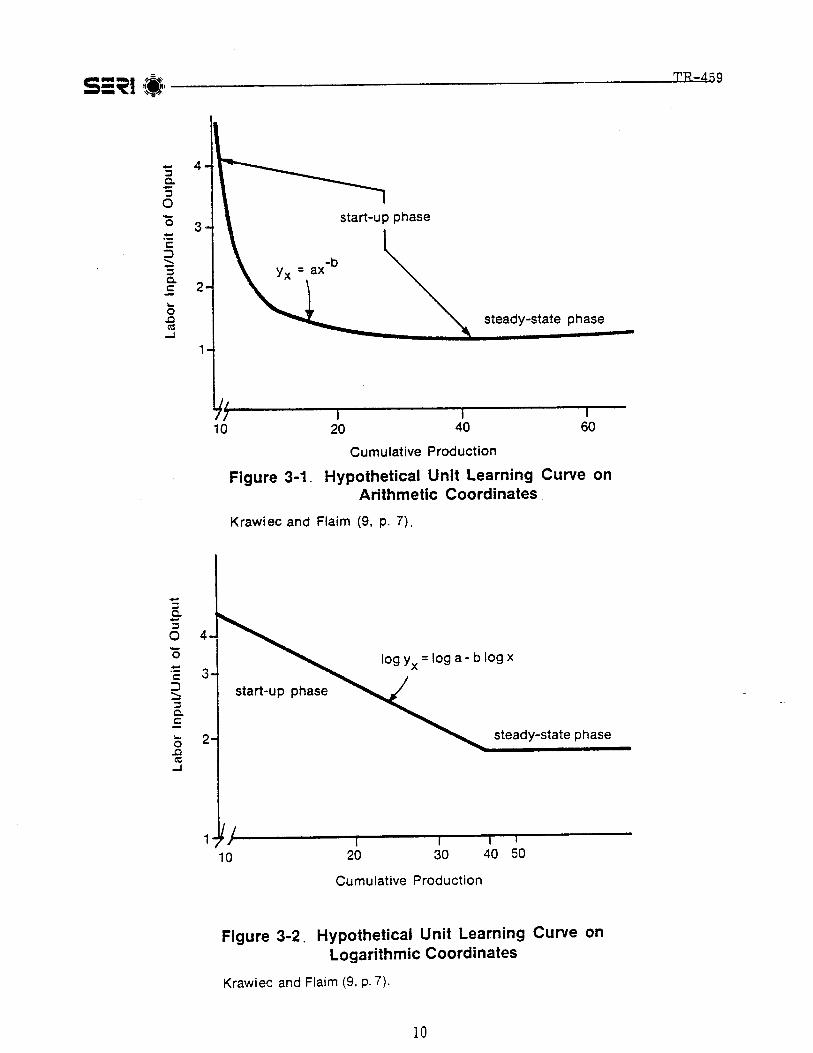
3-1 Hypothetical Unit Learning Curve on Arithmetic Coordinates...... •••.••.. 10

3-2 Hypothetical Unit Learning Curve on Logarithmic Coordinates.. . . • • • • • . . • • 10

3-3 Hypothetical Learning Curve on Logarithmic Coordinates. . • • • • • . • • • • • • • . • • 11

6-1 Schema fer a Typical Central Receiver System.. . . . • . • • . • • • • • • • • • • • • • • • • • 30

6-2 Heliostat Field and Central Power Tower. • . . • . . . • . . • . . . . • . . . . . • . . . . . .. .. • • 31

6-3 Cost Breakdown fer a Typical Central Receiver Plant. • • • • . • . .. . • • • • • • • • • . • 32

6-4 Typical Two-Axis Tracking Heliostat. • .. . • • • . • • • • .. • • • . .. • . • • . • . . • .. • .. .. .. • .. •• 32

6-5 Generic Heliostat Development 35

6-6 McDonnell Douglas Second-Generation Heliostat 36

6-7 Laminated Mirror Module Assembly. • .. . • • • . • . • • • • • • • • . • • • • • . • . • • • .. • • • • • • 40

6-8 Reflector Support Structure Assembly •...•.•.•..•.•.••••••••••••••••••• 41

6-9 General Electric Enclosed Heliostat 44

6-10 General Electric Heliostat Design 45

6-11 Stretch Frame Reflector Subassembly... • .• .•• .•.•. .•.. . .•••• •. •. •• •• •• • 46

6-12 Support and Drive Assembly •.•.•••••••••..•.•••.•.•••••••••••..•.••••• 47

7-1 Cumulative Heliostat Market Scenario. • • • • • • • • . • • • • • . • . • . • . • . • • • • • • • • • .. 53

7-2 Present Value of Capital Equipment 55

7-3 Block Flow Plant Layout... . . . .. . .. . .. . .. . .. • .. • .. . • • • .. . . • • • • • . • .. • .. • • • • • • . • . • . 65

7-4 Reflector Panel Assembly Manufacturing Flow... .• 66

7-5 Drive Assembly Manufacturing Flow. • • . • . • • • .. • • • • • • .. .. • .. • • • • . .. • • .. • .. .. . • . • 68

7-6 Final Assembly Joining Area Drive Unit to PedestaL..... . .••.. 71

7-7 Heliostat Controller Manufacturing Flow Chart 72

7-8 Data Distribution Interface (DDI) Manufacturing Flow Chart. • • . • . .. . .. • • .. • . . 72

7-9 Heliostat Control Harness Manufacturing Flow Chart 73

7-10 Installation Task Sequence. • • • . . . . . .. . . . .. • . . . • • . .. . • . • • .. • .. .. • .. .. • • • • . • .. • . .. • 75

xvii

TR-459S=~I :~I' ----------------------.....:..::.~=

LIST OF FIGURES (concluded)

7-11 Drive Unit Installation Machine ••••••••••••••••••••••.•••••••.•.••••.•• 77

7-12 Reflector Installation Equipment..... •••••••••• • ••• ••••••••• ••• ••• ••.• • 77

7-13 Cost Elements of MDAC Heliostat (25,000 Units/Yr) •••••• ••••• •• ••••• •••• 82

7-14 Cost Elements of MDAC Heliostat (250,000 Units/Yr) ••• • • •. • • • • • • • • •• • • • • 83

7-15 Cost Elements of MDAC Heliostat 0,000,000 Units/Yr) ••••••••••••••••••• 84

7-16 Cost Elements of GE Heliostat (25,000 Units/Yr) ••••••••••••••••••••••••• 90

7-17 Cost Elements of GE Heliostat (250,000 Units/Yr) •••••••••••••••••.•••.•• 91

7-18 Cost Elements of GE Heliostat 0,000,000 Units/Yr)....................... 92

7-19 Manufacturing Facility for 25,000 Heliostats/Yr) .•••••••••••••.•••••••••• 93

7-20 Manufacturing Facility for 250,000 Heliostats/Yr) ••••••••••.••.••••••.•.• 94

7-21 Typical Heliostat Installation Sequence. • . • • • • . • • • • . • • • • • . • . • • • . • • • • . • • . • 95

7-22 Unit Curve Plot. . . . . . . . . . . . . . . . . . . . . . . . . . . . . . . . . . . . . . . . . . . . . . . . . . . . .. 102

8-1 Heliostat Assembly Unit Cost Curve (GE) Design •••••••••••.•••••••.•.•.• 118

8-2 Heliostat Assembly Unit Cost Curve (MD) Design... •••• ••••• •• • •••••• •••• 119

xviii

TR-459S=~I 'IWII --------------------------­-~ ~~

LIST OF TABLES

4-1 Experience Curves Identified by the Boston Consulting Group

~

22

6-1 Technical Descriptions-Collector Subsystem ••.•.......•.••••••••••••••• 37

6-2 Drive Unit Requirem ents • • • • . • . • . • . • • • . • . • . • • • . . . . . • . • . • . • • • • • • • • • • • • • 42

6-3 General Electric Heliostat Weight Breakdown. . . • • • • • • • • • • • • • • • . • • • . • . • • • 48

6-4 Design Parameters Affecting Heliostat Elemental Cost.. . ..•.•.•.•••••• ••• 49

7-1 Prototype Heliostat Hardware Tree. • • • . . • • . • . • . • • . . . • . . • . • • . • • • . • • • • • • • 59

7-2 Installation Tasks and Crew Size ..••••..••••••.•••.••••••...•.••...•.•• 76

7-3 MDAC Prototype Heliostat Cost Breakdown •.•........•...•.•.•.•••••••• 81

7-4 GE Heliostat Cost Comparison. • • . • • • . • . . • . • • • • . • . • • . . • • • • • • • • • • • • • . • • • 87

7-5 Projected Costs for GE Heliostat Design ..••••••••••..••••••••.••••••••• 88

7-6 10,000 Heliostats/Yr Steady-State Preliminary Cost Breakdown ••...••••••. 89

7-7 Steady-State Costs.. . . . . . . . • . • . • . . . • . • . . . • . . . • . . • • • • • • • . • • • • • • • • • • • •• 100

8-1 Heliostat Design Components. • • . • • • . • • . • . . . . • . . . • . • . • • • • • • • • • • . • • • . • .• 106

8-2 Choice of Surrogates for Heliostat Components ...•..•••.•.•.••••.••••••• 107

8-3 Surrogates Used in the Study. . • . . . . . . • • • . . • • • • • • • . • • . • • • • • • • • • • . . • . • . .. 108

8-4 Cost Estimate-25,000th Unit, GE Design... •• •• •• . .•••• •••• •••• •• ••.• .•. 116

8-5 Cost Estimate-25,000th Unit, MDAC Design ••.•••.•.•••..••••••....•..• 117

8-6 Estimated Costs and Slopes fet" the MDAC Heliostat Design. • . • . • • • • • • . • • .. 120

8-7 Estimated Costs and Slopes for the GE Heliostat Design. • • • • • • • • • • • . • • • ••• 120

xix

TR-459~~11.'1, ------------------------------__~~.S=~I

SECTION 1.0

INTRODUCTION

A crucial issue in the commercial development of solar energy technologies concerns thecost of solar technologies and whether this cost can be reduced. Many solar technologiesare now too expensive to be economically feasible. Some of these technologies mayachieve substantial cost reductions with improved product design and production tech­niques.

An assessment of future solar energy costs* is necessary for several reasons. First, anassessment of solar technologies with the greatest potential for cost reductions wouldhelp establish research and development priorities. Second, such an assessment is usefulfor designing and evaluating government programs to accelerate the commercializationof solar energy. Finally, identifying possible reductions in costs leads to more accurateassessments of the potential market for solar energy.

Most of the U.S. Department of Energy (DOE) programs for estimating and predictingcost reductions in solar technology manufacturing have been through: (1) the low-costSolar Array Project at the Jet Propulsion Laboratory (JPL) and (2) the Repowering Strat­egy Analysis Supply Task of the Solar Energy Research Institute (SERI).

JPL has been investigating possible sources of cost reductions in all aspects of the pro­duction and assembly of flat-plate photovoltaic cells, including extensive SUbcontractingfor detailed design and engineering improvements in each step of the array productionprocess. This has led to refining a process to achieve the $2/Wp goal. Work remains tobe done in support of the $O.SO/Wp goal.

SERI has been analyzing the production economics of heliostats and investigating theeffects of changes in production quantity and processes on heliostat cost. Some changesin design and manufacturing processes may be necessary to attain low-cost, high qualityproduction. Also, SERI has been identifying significant cost components in heliostats andapplying these to an investigation of new heliostat concepts to determine the value ofthe new designs. A thorough bottoms-up engineering cost analysis has been performed.

The methods most often employed in past empirical studies to estimate and predict over­all cost reductions in manufacturing new products are: 0) engineering bottoms-up costanalysis; (2) engineering parametric approach; and (3) aggregate cost estimation tech­niques (short- and long-term cost functions, learning and experience curves based onbottoms-up engineering costs analysis, ete.). Cost estimates for solar energy technol­ogies typically are made assuming a fixed production process characterized by standardcapacity factors, overhead, and labor costs.

The concepts of learning and experience have been developed in the business manage­ment and industrial economics literature as ways to explain cost reductions observed insome industries; learning and experience curves were developed in order to estimate themagnitude of reduction in costs [9,10,12,13]. In the broadest sense, the concepts oflearning and experience are based on the premise that, as people gain experience withmethods of producing a particular product, improvements will be identified and imple­mented. Reductions in per-unit costs have been observed with such regularity in some

*Cost refers strictly to market cost in constant dollars, unless otherwise noted.

I

TR-4595=_~1 It.~~;,.,;;: ~~ ----------------------------_......=...:::.::-.=.::..::

industries that a number of authors believe that costs can be expected to decrease atsome constant, estimable proportion of cumulative production [26,27]. Because the solarindustry is relatively new, it could be argued that costs will decline as firms gain experi­ence with different methods of producing solar energy equipment [9]. Consequently, theobjective of this report is to assess the applicability of learning and experience curvesfor predicting the future costs of solar technologies. The major test case here is the pro­duction economics of heliostats.

A brief discussion of alternative methods for predicting cost reductions in the manufac­ture of new systems resulting from learning by doing, economies of scale, and technicalchange is summarized in Sec. 2.0. Learning concepts, including the factors affecting ini­tial production costs, procedures for estimating learning curves and their empirical appli­cations, and limitations of learning curves are presented in Sec. 3.0. Section 4.0describes the concept of experience and its applicability to cost estimation. Proceduresfor developing learning and experience curves for solar energy technologies are outlinedin Sec. 5.0. Section 6.0 summarizes the technical description of the McDonnell Douglasand General Electric heliostat designs and describes the basic elements of a solar centralreceiver system, the DOE heliostat development program, generic heliostat designs, andkey cost factors in heliostat designs. The factors influencing a costing scenario, a de­scription of the baseline production scenario, and steady-state production volume andcost variations are provided in Sec. 7.0. Section 8.0 describes the selection of surro­gates, derivation of learning and experience curves for surrogates, and application toheliostat assembly.

Appendix A contains a summary of the data acquired for the selected surrogate prod­ucts. An example of surrogate learning curve estimations is presented in Appendix B.Figures illustrating the cost curves for the MDAC and GE heliostat designs are providedin Appendix C.

2

TR-459S=~I ;.'1 --------------------------=-=~'-~ ~~,

SECTION 2.0

METHODS FOR PREDICTING COST REDUCTIONSIN THE MANUFACTURE OF NEW SYSTEMS

2.1 OVERVIEW

The rapid pace of technology development since the end of World War IT and improvedanalytical techniques are two of the reasons why analysts pay close attention to productcosts.

Alternative methods for predicting cost reductions in the manufacture of new productsinclude consideration of learning by doing; economies of scale; and technical change.The tools most often employed in past empirical studies to estimate and predict overallcost reductions in manufacturing are:

• engineering bottoms-up cost analysis;

• engineering parametric approach; and

• aggregate cost estimation techniques (short- and long-term cost functions,learning and experience curves based on bottoms-up engineering costs).

These methods, and the conceptual and analytical framework of learning and experiencecurves, are discussed in the following sections.

2.2 ENGINEERING BOTTOMS-UP COST ANALYSIS

The most widely used method to estimate cost in manufacturing a new product or systemis the engineering bottoms-up costs approach. This method has been successfully used toestimate manufacturing costs for various solar hardware systems [1-4]. Its analyticalframework is provided in detail in Ref. 1 and 2.

The hardware system design and performance specifications of the product, the produc­tion rates and schedules, and the location sites for facilities must be determined. First,equipment designs are evaluated to determine any potential manufacturing problems andto investigate the possibility of using less costly materials and processes. Make-versus­buy studies are conducted to determine availability and relative costs of outside sourcesfor components or subassemblies and the level of in-plant integration is determined.Proper equipment, tooling fixtures and auxiliaries are specified and the necessary facil­ities are laid out, and environmental impact studies and marketing and distribution anal­yses are completed.

Once this initial capital equipment and facilities cost estimate effort is completed, ini­tial engineering feasibility studies begin, followed by capital equipment and assessmentfacility cost. Capital equipment and facility costs are estimated by pricing manufac­turing and testing equipment, floor space and building needs, and unique tooling systemsoutlined in specifications. This costing process uses standard equipment manufacturingcatalogues, quotes, or estimates published in various manufacturing studies. The cost ofhighly specialized equipment and tools is usually determined from similar equipmentcosts. If necessary, escalation factors are applied to project these costs into the future.

3

TR-459S=~I.' -----------------------------~::..::.-:.:::..:

The next step is to estimate direct and indirect costs, including materials, labor, trans­portation, depreciation, and overhead.

Direct materials cost includes purchased parts, subassemblies, and all materials used tofabricate parts. The direct materials cost is stated in standard cost for parts manufac­ture. Material quantity standards are based on system/product specifications as to size,shape, appearance, desired performance characteristics, and tolerance limits. The de­tailed parts drawings and manufacturing specifications provide the required quantity forthe various materials and parts that make up the finished product. Direct materials costis based on market information. Reductions in direct material costs are estimated byanalyzing available quantity and lot discount rates for the total materials bill. Directmaterial cost is also affected by visibility, scrap and rework, and fee. The cost of pur­chased parts and subassemblies is mainly determined from vendor quotes for parts andsubassemblies and from catalog prices.

Estimates of direct labor cost begin with manufacturing specifications. They determinethe operations to be performed on the fabricated part and the time required to man thefactory equipment required to make the part. Industrial engineering methods (based onhistoric data obtained from similar products) and efficiency factors are applied to de­termine the person-hours required to complete each operation. Direct support hours forplanning, tooling, and product support are estimated by application of standard factors.Time required for materials handling and supervision is usually covered within the appliedburden rates. The direct labor cost is the product of person-hours in a given operationtimes pay rate. The sum of all the direct labor costs associated with each operationyields the total direct labor cost of producing a part. Hourly rates for labor are based onprevailing costs in similar industries for a particular region.

Indirect manufacturing costs include items such as supervision and clerical help, mate­rials handling, operating supplies, maintenance, janitorial work, process engineering,transportation, hand tools, quality assurance not included in inspection operations, andspare parts.

Transportation cost is determined from obtaining transportation costs of firms located inthe same region. Other indirect manufacturing expenses are included in the overheadrates. The amortization of the asset, return on investment, income taxes, propertytaxes, and capital repairs are included in the fixed-charge rate. The fixed-charge rateconverts capitalized cost into a series of uniform end-of-year payments to repay the in­vestment at the stated interest rate over the life of the asset.

Once this cost process is completed, the first unit cost of a given design concept, in­cluding material, labor, transportation, depreciation, and overhead, is estimated. Itspractical value is limited to providing a solid base for application of the aggregated costestimation techniques. The unit-cost estimate does not reflect an overall cost reductiondue to labor learning, economies of scale, and technological change over time. Becauseof the dynamic nature of cost reductions in manufacturing new products, generalizedstatements about specific cost data are meaningless. A thorough manufacturing costanalysis for a particular new product becomes complex when alternative cost reductiontechniques that have their basis in the engineering bottoms-up cost approach areconsidered.

4

TR-459S=~I · ·.i i -------------------------------­-~ ~~

2.3 ENGINEERING PARAMETRIC APPROACH

The engineering parametric approach combines scaling laws, direct analogy, cost factors,and cost estimating relationships (CERs) to estimate and predict cost reductions in man­ufacturing new products. Various government studies show this approach applies to com­munications equipment and advanced weapon systems. The most fundamental componentis the CERs. Based on engineering-economic theory basis and principles of statistics andeconometrics, cost estimating relationships are quantitative expressions of cause andeffect between cost, the dependent variable, and selected design and performance char­acteristics (e.g., weight, horsepower volume, material type, conversion efficiency) theindependent variables. G. H. Fisher and R. L. Petrushel present a broad description ofthe derivation of cost estimating relationships [5,6].

Detailed parametric costing relationships can be particularly useful for a new productduring its early phases of planning and development when only mission and performanceparameters are defined. These relationships can also be applied in evaluating manydesign options. During the early phases of a particular design concept, limited and un­certain physical and performance characteristics are available regarding new product de­velopment and manufacture. Therefore, relationships between aggregated components ofproduct cost and the physical or performance parameters of the product are derived fromcost histories on prior programs or from surrogate parts resembling the pieces to be man­ufactured in configuration, material, and production methods.

There are practical limitations to the engineering parametric approach. It is difficult toselect a surrogate part relevant to a given product component in terms of configurationsimilarity, material correspondence, and fabrication congruency. Even if the analogous,surrogate parts or subassemblies are truly analogous there are limitations inherent in sta­tistical inference. In addition, cost histories on prior programs are imperfect indicatorsof future costs of a given design concept.

2.4 AGGREGATE PREDICTION OF COST REDUCTIONS

The aggregate prediction of cost reductions in manufacturing new products involves anumber of conceptual and analytical issues associated with relationships between changesin a firm's costs and changes in its output; the cost function. Economic theories of theproduction function of a firm and the prices it pays for its inputs determine the firm'scost function. Since a production function may have different forms, with either one,some, or all of the input variables, cost functions may also have different forms. Pricetheory gives most of its attention, however, to two cost functions-the short-run and thelong-run. Since price theory is based on the neoclassical theory of the firm, the short­and long-run cost functions can provide insights into economic and technical issues thatinfluence the behavior of costs and prices over time. However, since neoclassical theoryof the firm is a static, or at best a relatively static depiction of behavior, it does notexhibit direct applicability of the short- and long-run cost functions to predict futurecost reductions. The cost functions have been extensively used in empirical studies ofproduction. Walters [7] provides a survey of applications of cost and productionfunctions.

The simplest short-run relation between changes in the costs of a firm and changes in itsoutput assumes that the fixed costs-those of the fixed plant and equipment, as well asthe state of technology of the firm-are constant. The firm's decision in the short run in­volves only determining the optimal quantity to produce. In the short run, fixed costs are

5

TR-459S=~II.'1i------------------------------=-=:..:.....::.:..:- ~~

relatively high, since little is done to achieve economies of scale due to expanded plantcapacity; improve economics of production technology and utilize optimum forms ofcurrent manufacturing techniques; introduce new production methods; and change the in­herent form of the product. Therefore, the only short-run manufacturing cost reductionsare those due to increasing labor productivity: (1) as workers repeat an operation, theylearn, and the number of person-hours required per unit of production declines; and (2)management techniques such as planning, purchasing, control, and supervision improve.Other variable costs may also decline as production increases. For example, direct ma­terials costs may be subject to volume discounts, more efficient purchasing, or reductionof rejects.

It is practically impossible to specify what the sources of short-run cost reduction will befor a new product. Therefore, in predicting cost reductions in manufacturing new prod­ucts in the short-run, the learning curve based on bottoms-up engineering costs has beenused as an approximation tool for future costs.

In the long run, all factors of production are assumed to be variable. The firm's pro­duction function has no fixed inputs; the firm has no fixed costs. Hence, the firm's long­run decision involves a simultaneous determination of the optimal level of output, as wellas the optimal mix of factor inputs. Greater opportunities exist in the long run for a costreduction in manufacturing of new products due to (1) technological change (Le., substi­tution of more efficient production equipment, processes, or products for less efficientones); and (2) economies of scale (i.e., expanded plant capacity, increased labor effi­ciency resulting from worker specialization, or more efficient combination of productionfactors). Changes in scale, technology embodied in the fixed capital, and the inherentform of the product occur gradually. Consequently, the long-run cost function reflectsunit cost changes that are relatively smaller than those of the short term.

To estimate cost reductions in the manufacturing of a new product, the experience curveconcept is applied as an aggregate tool to summarize cost changes resulting from a num­ber of different long-run sources. This concept has been applied because it allows ap­proximation of future manufacturing costs. Although of great practical importance, it isnot possible to estimate the relative proportions of total decrease in unit cost that arecaused by changes in long-run cost reduction sources, or to characterize the manner inwhich unit cost changes occur separately from changes in the specified long-run cost re­duction sources. It is not feasible to anticipate with any real accuracy how or why thecosts of any specific product are going to change in the future.

6

TR-459S=~I 1'.'-------------------------~-~ ,~~

SECTION 3.0

THE CONCEPTUAL FOUNDATION OF LEARNING

3.1 BACKGROUND

The learning curve is a generalization about the sources of short-run cost reductions. Aliterature survey of learning curve applications [8,9,10] indicates that different authorshave presented a wide variety of definitions of the sources of cost reduction in manufac­turing new products that are generalized in this phenomenon. There is no consensus inthe literature as to whether a given process innovation will result in a shift in thelearning curve or a movement along the curve. This distinction is of critical importancefor policy makers.

Any changes in variable inputs to the production process are defined as modifications ofa given process and hence a movement along the learning curve. Variable inputs arethose production factors whose cost varies with short-term fluctuations of output. Anychange in fixed inputs to the production process is defined as a switch in processes and,hence, a shift in the learning curve. Fixed inputs are production factors in which costdoes not vary with short-term fluctuations of output. Thus, improvements in the effi­ciency or organiaation of the work forces, management, or other variable inputs are re­garded as movements along the learning curve. Changes in scale or technology embodiedin fixed capital are considered shifts in the learning curve. This definition makes move­ments along the learning curve analogous to short-run adjustments in traditional eco­nomic theory and shifts in the learning curve analogous to long-run adjustments. Theseparation of those sources causing shifts in the learning curve from those causing move­ments along the learning curve, allows a precise distinction to be made between the ex­perience concept and the learning curve effect. Also, policy recommendations are maderegarding optimal actions to take to ensure the achievement of cost goals.

The learning curve is considered here to be an aggregate tool that empirically summar­izes the sources of cost reductions in manufacturing new products within one particularprocess.

The experience curve herein is restricted to the analytical tool that collectively general­izes the shifts in the learning curve that result from changes in scale or technology em­bodied in fixed capital.

This section extensively discusses the definition of learning, approximation function, pro­cedures for estimating learning curves, empirical applications of learning curves, andlimitations of learning curves, in addition to the conceptual foundation of learning.

3.2 DEFINITION OF LEARNING

The expression itself is borrowed from psychology, which has found through experimenta­tion that humans and many animals learn at certain rates by repeated trials.

The conceptual foundation of learning observed for manufacturing operations originatedaround 1920 in the aircraft industry and was subsequently reported by T. P. Wright in1936 [17]. Its basic concept, that the direct labor input required to produce each of aseries of airframe orders for a particular plane model diminished at a uniform rate as the

7

TR-459S=~I 'Il' --------------------------------

orders accumulated, is still accepted theory. During subsequent years, it was found that,once production on a plan commenced: the fourth plane required only 80% as muchdirect labor as the second; the sixteenth plane, only 80% as much as the eighth; thetwentieth, only 80% as much as the tenth; and so on. Based on this uniform pattern, itwas concluded that the rate of learning to assemble aircraft was approximately 80%between doubled quantities.

The learning concept, its properties and uses, has been the subject of extensive study anddiscussion [8-16] producing relevant data and theoretical knowledge of the subject. Thelearning concept, also called manufacturing progress function [8], is presently used tocharacterize an increasing labor efficiency: again, as workers repeat an operation, theylearn, and the number of person-hours required per unit of production declines; the effi­ciency improvement is regular and predictable [11, p. 410]. This definition has been usedin various empirical studies [8,9,11,14-16]. Conway and Schultz state that it "holdspromise of providing a better basis for the budgeting of engineering and other efforts incost reduction activities, for the budgeting of production vs. product engineering, andpossibly for providing some objective indication of organizational achievements" [8,p. 39].

Variations of the preceding learning phenomenon definition used by a number of authors[12, pp. 25-27; 10, p, 24] are of relatively limited value because of the conceptual andempirical uncertainty involved [9, p, 4] •

The defined concept of learning emphasizes an increased direct labor efficiency as theprinciple causal factor in short-run manufacturing cost reduction. Conway and Schultzbelieve that "operator learning in the true sense of performance of a fixed task is of neg­ligible importance in most manufacturing progress" [8, p. 42] , although it significantly in­fluences the number of subsequent opportunities for cost reduction. In most industriestooling changes, redesign of production methods, and improved management techniquessuch as planning, purchasing control, and supervision are more important sources of costreduction than direct labor learning. "Such changes are usually the result of managementand engineering effort rather than operator learning in any sense" [8, p. 42].

In this report, a learning concept is restricted to mean improved productivity of a directsingle input (e.g., labor).

3.3 THE LEARNING CURVE

A curve depicting the learning curve concept "was worked up empirically from the two orthree points which previous production experience of the same model in differing quan­tities made possible" [17, p. 122]. To represent the functional interdependencies betweenlabor hours per unit of output and cumulative production, the following approximationfunction is suggested [8,16J:

Y - xa-bx- (1)

where

Yx = labor hours required to produce the xth unit of production;

x = cumulative production, between l st and xth units;

a = estimated labor hours required to produce the 1st unit; and

8

TR-4595=~1 1.1 ------------------------------­-~ ~~

b = a measure of the rate of reduction in labor hours as cumulative produc­tion increases.

Parameter a is obtained by extrapolating the learning curve to x =1. If x =I the numer­ical value of the parameter a is given by:

y1 =a(U-b =a •

The numerical value of the parameter b describes the rate of decrease in direct laborinput only of a new product. Its past values have normally been in the range -1 < b < O.

The logarithmic transformation of Eq. I is:

log Yx = log a - b log x

which is a straight line when graphed on logarithmic coordinates. Figure 3-1 portrays ahypothetical learning curve on arithmetic coordinates; Fig. 3-2 illustrates the same curveon logarithmic coordinates [9, p. 7].

The learning curve applies only to the range of production over which learning occurs[8,15,16]. In actual experience, a given operation eventually approaches a plateau or asteady-state phase, during which direct labor input remains constant as cumulative pro­duction increases [8,16]. This is often encountered with large output volume. In prac­tice, this phase should be estimated independently U6, pp. 330-331]. The start-up andsteady-state phases are illustrated in Fig. 3-1 and 3-2.

In practice, the rate of reduction in labor hours is often replaced by the learning-curveslope, that is, "the percent of learning that occurs each time output is doubled" [16,p. 330]. The learning-curve slope is often called the progress (pI) [I6, p. 330]. Its math­ematical expression is defined as follows:

if Xl and x2 are two points in production and x2 =2xI ,

-bY2 aX2 -b

then PI = --- = --=b = 2Yl ax-

I

(3)

or b =log PI/log 2 •

The rate of reduction is usually described by giving the complement of the r~duction thatoccurs when the production quantity is doubled. This is equal to the PI = 2- Hence, inan estimated learning curve with b equal to -0.322, its PI would be 80% (2-0.~22 =0.80),indicating that each time production output doubled the direct labor input would be re­duced to 80% of its for mer value.

The learning curve defined by Eq. 1 is called a unit curve. In practice, a cumulativeaverage curve is often applied [8,16,18].

I

9

TR-459S=~I '.~I-----------------------------...::..:..:..-- \~."

It is characterized by the following approximation function [8, p. 40]:

-bx (4)

where

Yx = cumulative average labor input per unit, averaged over all units of produc­tion from the first to the Xth.

x = the production count (x =1, 2, ••• , X).

N = cumulative production between the 1st and Nth unit.

All other symbols are the same as in Eq. 1.

For values of N greater than 100, Eq, 4 can be approximated by [12, p. 40]:

-bax1 - b

where all symbols are the same as in Eq. 4.

The various empirical studies [19-22] report substantial difficulties in determining thepragmatic superiority of the preceding curves by logic and empirical evidence. Conwayand Schultz observed that "the choice in usage has been largely a matter of computa­tional convenience; when the unit curve is of primary interest and use, the first model isselected; when the cumulative average curve is primary, the alternative model is used.Since in either case the two curves are parallel for large quantities of production the dif­ference is important only during the initial stages of production and hence for manyapplications, not crucial" [8, p. 41]. Figure 3-3 illustra tes two hypothetical curves drawnon logarithmic coordinates. The upper curve shows the cumulative average curve, whilethe lower line represents the unit curve.

In applying the cumulative average curve, an analyst should keep in mind that "the aver­aging process has tremendous power to smooth the data and enhance the appearance ifnot substance of the curve" [8, p, 41] .

Although learning in the literal sense here is restricted to improved productivity ofdirect labor input, the learning curve is an analytical tool applied to generalize the com­bined effects of both increased efficiency of workers and management innovations [15,p. 89].

3.4 LEARNING CURVE ESTIMATION

The method used to estimate the learning curve structural parameters depends upon thenature and format of the data required. The use of the learning curve as a predictor re­quires some clear definition of the quantitative measures relating to the variables used inestimating its structural parameters. The variables used in estimating learning curve

12

TR-459S=~I "*, --------------------"'---------~ ~<

structural parameters (i.e.; the estimated direct labor input required to produce the firstunit and the rate of reduction in direct labor input) are: direct labor hours required toproduce the xth unit of production and cumulative production between the first and xthunit.

It is imperative that accurate, reliable, and properly aggregated "data be used for eachvariable. Conway and Schultz summarize the difficulties encountered in obtaining theproduction count.· The most important are [8, pp. 43-44]:

• Varying lot sizes, lead times, and schedules make it difficult to associate specificcosts with specific production quantities of the end product.

• Some components are produced in relatively large volume in initial lots and la terare split in production.

• Actual labor times are seldom accurately recorded; considerable doubt exists asto the validity of operator times charged to direct vs. indirect labor accounts.

• Actual product costs in terms of dollars or labor time are, in many cases, unob­tainable.

• Design and model changes make it difficult to judge if a change is significantenough to justify treatm ent of the product as a new model, and when it should betreated as normal progress with the current model.

• Definition of individual operations is not constant over time; a particular portionof the work that must be performed on each unit often shifts from one operationto another.

Some of these difficulties can be eliminated through the process of aggregation of theparts manufacture operations and subassembly and final assembly operations. Conwayand Schultz state that "considering the sum of two operations the data are unaffected bywork transferred between these two operations (assuming the times for elements areadditive). Considering the product as a whole, redefinition of operations does not affectthe data. n••• in considering groups of operations we are in effect considering the sumsof a number of chance variables. In general such sums are much better behaved than theindividual change variable" [8, p, 43-44]. However, they indicate that the aggregationprocess applies only to those operations that have basically the same cause-and-effectpa tterns [8, p. 44]. Thus, each operation, part, subassembly, and assembly that has dif­ferent cause-and-effect patterns is subject to its own learning curve.

Once the selection and aggregation process is complete, quantitative measures relatingto the cumulative production count and the direct labor input required to produce the xthunit of production should be determined. The three quantitative measures that an ana­lyst can develop, based on sufficient data, are:

• The sequential production units and corresponding actual direct labor input forany particular unit.

• Production lot sizes released and corresponding costs accumulated on a produc­tion lot basis. The mean of a lot and corresponding average direct labor input iscalculated. An average direct labor input is weighed by the amount of produc­tion it represents.

• An annual cumulative production and corresponding cumulative average directlabor input, averaged over all units of production.

13

TR-459S=~I "r.'-~, --------------------------------- '~~

After these measures are established, the learning curve can be developed either graph­ically or mathematically. In applying the former process, the log paper is used to plot adirect labor input per unit against cumulative output. The line that connects these pointsis the learning curve for the units produced. The slope of the line indicates the percent­age of direct labor input reduction achieved as the number of units produced is doubled.Alternatively, mathematical curve fitting procedures are applied to estimate whichequation best fits the data points collected. In applying this approach, the exponentialapproximation function is assumed. On the basis of the empirical data, an analyst esti­mates the function's structural parameters by application of the ordinary least squaresmethod.

Although the exponential function is the most widely used functional form, it has not yetbeen logically or mathematically rela ted to manufacturing procedures in terms of quanti­tative cause and effect. This form is intuitively appealing because it reflects the factthat, in some industries, progress is rapid during the early stages of production and con­tinues at a decreasing rate [15, p. 89]. Several authors proposed alternative approxima­tion functions such as log-quadratic. Orsini summarizes this debate, the results of whichhave been inconclusive [13, pp, 24-30]. Krawiec and Flaim state that "since the logic be­hind the learning concept does not suggest a particular functional form, analysts shouldspecify an equation which best summarizes the data" [9, p. 10].

Perhaps the most difficult problem associated with estimating learning curves is aggre­gation. The production of a given product is not a single process, but rather a summationof fabrication, processing, subassembly, final assembly, installation, and testing, subjectto its own learning curve. The aggregated learning curve for a given product is the ver­tical sum of the individual unit learning curves. The process of aggregation of the indi­vidual unit learning curves rests on a strong assumption that the exponential approxima­tion function (which is linear in logs) holds for each manufacture, subassembly, and finalassembly operation as well as for the completed product. It is difficult to justify as­suming such linearity. Conway and Schultz indicate the implications involved by consid­ering the sum of two unit learning curves for a series of two components of a given endproduct:

(5)

a plot of (YL + Y2)x against x on log coordinates is a convex curve whose shape depends onthe values tal' a2' bl, and b2). The plot will be straight if and only if b1 = b2 = b[8, p. 41]. This indicates that the rate of learning is the same for both components,which will not generally be the case. Theoretically, the exponential learning curve canat best apply to only one level [8, p. 41]. Krawiec and Flaim indicate that "from apractical point of view, aggregating learning curves for processes involves complex cal­culations. If analysts decide to use the exponential function for each suboperation andthen the sum for convenience, they should realize that doing so will result in errors incomputation" [9, p. 11].

An alternative approach is to calculate the actual cost of the first unit "as a basis forextrapolation and use of a uniform 80% characteristic to define slope" [8, p. 44]. The

14

TR-459S=~I I I.~ 1 ---------------------------~ ,~,

first unit cost, the basic parameter to loea te the function, may be defined in a number ofways depending on the perspective of the analyst. In a development firm, it may beviewed as the cost of the first test article with or without a nonrecurring engineeringallocation or as a synthetic value extended from industrial engineering standards thathave been determined at, say, the lOath unit of production. Development of the firstunit cost can be accomplished employing the engineering build-up cost method "on thebasis of rome implicit conception of stabilized production volume and conditions peculiarto the firm and its environment" [8, p, 44]. The applicability of this approach to estimatenumerical values of the structural parameters of the function is questionable. Althoughthe approach is widely used in the aircraft industry, Conway and Schultz do not recom­mend its application because "There is no such thing as a fundamental law of progresssuch as the '80% learning curve'..•. No particular slope is universal, and probably thereis not even a common model" [8, p. 53].

Despite the various difficulties and unsolved problems mentioned, the structural param­eters of the specified approximation function can be estimated either graphically ormathematically.

3.5 EMPIRICAL APPLICATIONS OF LEARNING CURVES

The learning curve was developed as a managerial planning tool. It has been used as abasis for facilities and manpower scheduling, pacing assembly operations, and cost esti­mation [8, p. 50]. Cost estimates obtained through learning curves have been used as thebasis for contract negotiations in the aircraft industry, and for a variety of pricing,buying, and financing decisions [15, pp. 91-95].

Estimated learning curves can be useful tools for predicting manufacturing costs. At thecenter of empirical studies is the concept of separating labor, materials, and overheadcosts, the factors that make possible both cost reductions and concomitant increases inquantities produced. Prediction of labor costs will be discussed first. Next, the estima­tion of the parameters of the curve for materials and overhead costs will be considered.Then, procedures for obtaining total product costs will be outlined. Finally, the limita­tions of learning curves will be addressed.

3.5.1 Labor

A learning curve indicates the relationship between labor input (measured in labor hoursper unit of output) and cumulative production. In order to determine labor costs, laborhours must be multiplied by appropriate wage ra tes. Even though some authors have usedlearning curves to predict labor costs directly [13,14], labor hours and wage rates shouldbe calculated separately for several reasons.

First, economic theory suggests that as the productivity of an input increases, its wagerate should also increase [23, pp. 293-307]. Second, for some of the industries examined,Conway and Schultz found that progress in labor hours was roughly offset by rising hourlywages and that labor costs were less predictable than hours [8, p, 491. They state:

Use of labor hour or a machine hour base has been found to be much moreilluminating than dollar costs. Where dollar costs are desired they may beused as a multipli er, but price changes serve to mask production progress interms of fundamental resource consumption. [8, p. 53]

15

TR-459S=~I.'-------------------------------Finally, labor hours can be reduced by substituting more skilled and more expensive laborfor less skilled workers. However, reducing labor hours could cause higher labor costs[15, p, 90]. For these reasons, labor hours and wage rates must be calculated separatelyto avoid errors in labor cost predictions.

3.5.2 ~aterials

Material generally decreases in cost as the quantity of output increases. Although theestimation of the parameters of the curve for materials costs has been of significantconcern, little has been written concerning reduction in the materials component ofproduct cost. Only a few authors have examined materials cost reductions due to volumediscounts, more efficient purchasing, or reduction of rejects [17,18,20,24]. Conway andSchultz believe that "there is no reason why one could not quantify past experience anduse it to predict reduction in materials cost. Lacking such information, one would prob­ably neglect progress in this area except for obvious economics associated with quantity"[8, p. 51].

3.5.3 Overhead

Some empirical studies indicate that amount of overhead varies, within limits, with quan­tity of output. Overhead is usually expressed as a percentage of direct labor costs thatresults in a log-linear relationship for overhead costs. Overhead costs fluctuate greatlyin different cases depending, for example, on structural components (i.e., taxes, depreci­ation, executive salaries) or when a particular factory is engaged in the manufacture ofone or many types of products [17,24].

3.5.4 Obtaining Total Produetion Costs

An aggregated cost curve for direct application to different quantities of the end productcan be developed by combining factors of labor, material, and overhead. Wright pointedout that the shape of a total cost curve developed by this method in the aircraft industry"will start out at 83%, then change to 87%, and finally reach 90%. This change in slopeis an indication of the relatively greater importance of material to labor as quantity in­creases" [17, p, 126]. This cost estimation procedure is distinctly different from usingexperience curves to predict total unit costs directly.

3.6 UMITATIONS OF LEARNING CURVES

Learning curves can be useful tools for estimating changes in production costs. Theyhave been applied successfully in aerospace and related defense industries [8,15-17]. Therelevance of the learning curve in labor extensive manufacture-automobile assembly,apparel manufacture, and the production of large musical instruments-was found byBaloff', The studied products, modes of manufacture, and industries differed significantlyfrom each other and from the aerospace industry to suggest a greater, wider applicationof the learning curve model in labor-intensive production activities [16, p. 339J. There isneed for a greater generalization for and application of the learning curve model incapital-intensive industries. Labor learning as defined here may only be a minor sourceof cost reduction in these types of production activities. However, the literature[8,14-17,24] does not provide empirical evidence questioning the applicability of the

16

TR-4595=~1'(·:------------------­-~ .learning curve concept in capital-intensive industries. These learning curves are subjectto three important limitations.

First, the learning curve is a method of estimating changes in labor productivity whichoccur after production operations begin. If substantial efforts are devoted to preproduc­tion engineering and planning and if labor productivity is higher than it otherwise wouldhave been, the learning curve will not capture the progress that has been made.

Second, learning rates vary substantially among industries, firms, products, and types ofwork [8,14,16]. Again, Conway and Schultz conclude:

There is no such thing as the fundamental law of progress such as the "80%learning curve"* used in the aircraft industry. No particular slope isuniversal, and probably there is not even a common model. The contentionthat such exists is most difficult to defend either logically or empirically.[8, p. 53]

Analysts must choose the appropriate model and estimate the rate of progress for thatproduct.

Third, the analyst must determine the range of production over which progress willoccur. Empirical data show that progress does not continue indefinitely [8,16,26]: Theapplication of learning curves is based on the assumption that progress in labor hours willbe achieved over the range of production specified.

*The "80% learning curve" is identical to the progress index.

17

18

TR-459S=~I11*;1 -----------------------------=...::.:...~~

SECTION 4.0

THE CONCEPT OF EXPERIENCE*

Like the learning concept, the experience concept was developed from the observationthat per-unit production costs declined in some industries as a direct, estimable propor­tion of cumulative production [26-28]. Unlike learning that refers to the productivity ofa single input, the experience concept has been used to describe changes in total cost asa function of cumulative production.

According to the Boston Consulting Group, which claims to have originated the concept,"The experience ••• effect .•• encompasses all costs (including capital, administrative,research, and marketing) and traces them through technological displacement and prod­uct evolution" [27, p. 6]. They state from their observations of various industries that"Costs appear to go down ••• 20% to 30% every time total product experience doublesfor the industry as a whole, as well as for individual producers" [27, p. 12]. The experi­ence concept appli es to long-term improvements in production processes and includescost reduction from every conceivable source, including technical improvements, inputsubstitution, economies of scale, new product design, and changing input prices.

4.1 EXPERIENCE CURVES

Experience curves are similar to learning curves and are calculated as follows:

c = axbx {6}

where

Cx = the cost of producing the xth unit of output;

x = cumulative production;

a = estimated cost of producing the 1st unit; and

b = parameter measuring the change in total cost (normally, -1 < b < 0 isassumed).

In practice, the experience curve usually refers to the percentage reduction in cost thatoccurs when cumulative production is doubled. It is calculated the same way that theprogress index is calculated for learning curves:

(7 )

-baX2 -b

-b = 2aXl

An 80% experience curve would indicate that if cumulative production doubles, per-unitproduction cost would decline to 80% of its level prior to doubling [28, p, 53].

*This section originally appears, in essence, in Krawiec and Flaim [9].

19

TR-459S=~I ,Ii, --------------------------"'-..........~

4.2 APPUCATIONS OF EXPERIENCE CURVES

The Boston Consulting Group (BCG) examined historical data for 24 products and foundthat price reductions* were strongly correlated with cumulative production [27, pp. 69­101]. Their results were summarized by Costello et ale [10] and are presented in Table4-1. Similar data were compiled by Hirschman [26] and cited by Bodde [28].

These experience curves were not estimated by the BCG to be used directly for cost esti­mation purposes. Rather, the BCG and other authors cite experience curves as evidencethat costs can decline as the result of many factors; they recommend that managers beaware of cost reduction possibilities when designing product-market strategies [26-28].

4.3 EXPERIENCE CURVES AND COST ESTIMATION

Even though cost prediction was not the goal of the Boston Consulting Group, some ana­lysts have attempted to use experience curves to predict the future costs of solar tech­nologies [24, pp, xiv-xv, 159-161]. Despite the statistical evidence that costs have de­clined in some industries, there are serious problems with using experience curves topredict cost reduction.

One problem is that there is no logical reason to believe that costs should decline as afunction of cumulative production per see In other words, there is no a priori reason tobelieve that the parameter b in the experience curve will have a negative sign. It isquite possible that costs may be increasing for a particular product. Long-run costscould increase due to rising input prices, government regulations requiring higher costproduction methods, or firms adopting new production methods that result in higher pro­duction costs.**

A second problem is that there is no way to separate cost changes due to technical prog­ress from those due to falling input prices, because the experience curve describes costchanges as a function of cumulative production. Declining input prices clearly influencedcost changes for at least 9 of the 24 products cited by the BCG: electricity and the 8 pe­troleum-based products.f Experience curves necessarily reflect the combined effects ofboth progress and declining input prices, and cannot be interpreted as measures of prog­ress alone.

*Cost data were unavailable; price data were used as proxies for costs. Price changeswere measured in constant dollars. In general, prices are inadequate measures of costbecause prices are determined by both supply and demand conditions.

**Firms might adopt higher-cost (less optimal) production methods because of imperfectinformation or uncertainty. In addition, if markets are not price competitive, firms maypursue goals other than cost minimization, which could result in higher production costs[30]. However, these factors are beyond the scope of this report.

,r Crude oil prices in constant dollars generally declined from 1950 to 1972 (see Table4-1). Crude oil is an input to petroleum products; fuels derived from crude oil are used inelectricity generation.

20

TR-459S=~I ,[II ------------------------------:..:.::...~~

Separating the influence of technical progress from that of changing input prices isfurther complicated by the fact that both affect improvements in production processes[31, p. 23]. Thus, if a change in the production process is made in order to substitute acheaper input for a more expensive input, that improvement cannot be expected to applyto a solar technology unless the solar firm faces the same relative input prices.

The third problem involves source identification and analysis. Even though the experi­ence concept as defined by BeG [27] and Bodde [28] includes cost reductions from logicalsources such as technical improvements, sources of cost reduction must be identifiedseparately and their impacts on costs must be analyzed directly. There is no other wayto evaluate whether cost reduction sources and their impact on costs can be expected toapply to the production of solar technologies. Without careful analysis of these separatesources, experience curves that are estimated from other product histories and used topredict the future costs of solar technologies will yield arbitrary and perhaps misleadingcost estimates.

Analysts using experience curves to predict future costs of solar technologies should heedthe advice of the Boston Consulting Group, who origina ted the concept:

As a practical matter experience curves should be considered only as ameans of understanding relationships, not as a measuring device. There areinherently too many difficulties in definition and factor measurement. Thisapplies particularly to the definitions of product and cost as well as meas­uring accumulated experience. [27, p. 63. Emphasis addedJ

21

TR-459S=~II_I----------------------------

Table 4.-1. EXPERIENCE CURVES IDENTIFIED BY THEBOSTON CONSULTING GROUpB-

(Cumulative Industry Production vs. Price)

Experience CurveProcess or Slope DataIndustry (Constant Dollars) Comments

Germanium Transistors 90% (1954-1960) 1954-1968Industry 70% (1960-1968) 1954-1969

Silicon Transistors Industry 90% (1954-1959) 1954-196970% (1960-1965)80% (1965-1969)

Germanium Diodes 90% (1955-1959) 1955-196870% (1960-1968)

Silicon Diodes 90% (1955-1959) 1955-196870% (1960-1968)

Integrated Circuits 70% 1964-1968 0965 &1966 monthly data)

Crude Oil Increasing prices 1946-1968(1946-1948) real prices90% (1948-1958) increased from70% (1958-1968) 1946-1948

Motor Gasoline Prices increased 1946-1968(1946-1949) (average price/90% 0949-1957) gal. excluding75% (1957-1968) California)

U.S. data only

Ethylene 100% (1953-1963) 1953-196870% (1963-1968) U.S. tariff price

vs. U.S. data only

Benzene 70% (1953-1963) 1952-196890% 0963-1968) U.S. data only

Paraxylene 90% 0957-1961) 1957-196870% (1961-1968)

Low Density Polyethylene 90% (1952-1959) 1952-196870% (1960-1968)

Polypropylene 90% (1959-1961) 1959-196880% (1961-1968)

Polystyrene (General Purpose 90% 0943-1954) 1943-1968Molding and Extrusion Resin) 70% 0954-1968)

Polyvinylchloride 90% (1946-1955) 1946-19687096 (1955-1961)80% 0961-1968)

22

TR-459S=~II.}I-----------------------------

Table 4.-1. EXPERIENCE CURVES IDENTIFIED BY THEBOSTON CONSULTING GROUpa (concluded)

(Cumulative Industry Production vs. Price)

Process orIndustry

Experience CurveSlope

(Constant Dollars)Data

Comments

Primary Aluminum

Primary Magnesium

Titanium Sponge

Monochrome TelevisionReceivers

Total FreestandingGas Ranges

Total FreestandingElectric Ranges

Facial Tissue

Japanese Beer

80% (1929-1939)70% (1939-1948)no trend (1961-1968)

80-90%

100% (1950-1954)70% (1954-1968)

90% (1947-1954)70% (1954-1968)

100% (1946-1950)70% (1951-1967)

90% (1946-1957)70% (I957-1967)

90% (1933-1945)increases (1945-1948)90% (1948-1966)

80-90%

1929-1968

1929-1968significantdeviations in trend

1950-1968strong devia tionbetween 1958-1968

1947-1968

1946-1967average wholesaleprice

1946-1967

1933-1966

1951-1968retail priceminus indirect tax

Electric Power

Re fined Cane Sugar

70% (1939-1943)80% (I943-1968)

70%

1930-1968

1935-1968very wide fluc­tuations in data

aFrom Costello et ale [l 0, pp. 32-33]. Data were compiled from Boston Consulting Group[27, pp. 69-110].

23

24

TR-459S=~I ;.~I--------------------------------~ ~'

SECTION 5.0

DEVELOPMENT OF LEARNING AND EXPERIENCE CURVESFOR SOLAR ENERGY TECHNOLOGIES

5.1 BACKGROUND

The crucial issue in the commercial development of solar energy technologies is: "Howwill the cost of solar technologies change over time?" Many current solar technologiesare too expensive to be economically feasible. Some of these technologies may achievesubstantial cost reductions from improvements in product design and production tech­niques. These cost reductions are usually estimated or predicted on the basis of roughcomparisons in dollars/lb or by comparing similar products. While such predictions mayindicate a general cost range, they are of little value in making investment decisions ateither the public or private levels in identifying specific areas needing improvement.

A brief and simple method for predicting the effect of future changes in design, mate­rials, or production methods of solar technologies is essential to optimum developmentand planning.

An analyst can estimate future normal costs of a given technology or product if heunderstands their basic relationship to learning and experience. Such a relationship canbe quantita tively expressed by the application of learning and experience curves.

5.2 DATA LIMITATIONS

Empirical applications of learning and experience curves have been based upon productsfor which production data are available [8,12-14,16,17,26,27]. However, solar energysupply systems represent emerging technologies with both mature components and proc­esses and untested prototype parts, assembly methods, and installation processes. Manysolar technologies require significant amounts of on-site construction. Most learning andexperience curves have been developed for the products that were manufactured, ratherthan constructed on-site.

Since the solar industry is young, few data are available on production economics andhardly any basis exists for estimating a partloular learning or experience curve slope. Insuch situations, learning and experience curves must be based on surrogate products orsystems resembling solar products in configuration, materials, and production methods.The selection of an appropriate surrogate product or system with an available cost his­tory allows inferences to be made regarding the cost of the new product. It is assumedthat because of these similarities, the new product will undergo the same cost reductionpa ttern as the surrogate product. Procedures for developing learning and experiencecurves for new products or systems using surrogate data follow.

5.3 ESTIMATING LEARNING AND EXPERIENCE CURVES FOR SURROGATEPRODUCTS OR SYSTEMS

The procedure begins with the conceptual disaggregation of the new product or systemassembly into components, subassemblies, and processes. This disaggregation dependsupon the analyst's concept of availability of relevant surrogate components, subassem­blies, and processes.

25

TR-459S=~I '.,------------------------ ~~

The surrogate part or subassembly should then be identified. A number of selected surro­gates might later be eliminated because of special circumstances in their commercialdevelopment, the fact that some entered the market fully developed, and the lack of re­liable historical cost data.

The third step is to collect historical data on the costs of each of the surrogate parts orsubassemblies and to break down these costs according to labor, materials, and over­head. Labor input should be measured in person-hours per unit of output, multiplied byappropriate wage rates, in order to determine labor costs. Economic theory suggeststhat as the productivity of a labor input increases, its wage rate should also increase [23,pp. 293-307]. For some of the industries examined, Conway and Schultz found thatprogress in labor hours was roughly offset by rising hourly wages and that labor costswere less predictable than labor hours [8, p. 49]. Labor hours can be reduced by substi­tuting more skilled and more expensive labor for less skilled workers; however, by re­ducing labor hours, a firm could face higher labor costs [I5, p. 90]. "For these reasons,labor hours and wage rates must be calculated separately to avoid errors in labor costpredictions" [9, p, 13]. Material inputs should be measured in both physical units anddollar-cost-per-unit. Unit overhead cost should be expressed in dollars, and individualelements of the costs generated should be corrected to eliminate the effects ofinflation. Production volume for surrogate parts and subassembly should also bedetermined.

Historical data collection for surrogates is the most difficult task, not because generalinformation does not exist, but because detailed data concerning labor, labor costs,material costs, and investment on a historical basis may not exist in some instances, maybe extremely sensitive in others, or may be so interspersed with other unrelated data asto be either unusable or uncollee table, Most of the data involved, except for regulatedindustries, are usually unavailable to the public. But it is not always necessary to usecurrent or recent proprietary data sources to establish trends. An analyst can use pub­lished retail or wholesale manufacturing data to break down information into its cost­specific components. He can then juxtapose specific technological improvements madein particular industries with new data. However, this process requires tremendousamounts of time and effort.

Once the data are obtained, an analyst has to identify the technological factors thatcaused specific manufacturing changes or trends for the selected surrogates and deter­mine how this development would or would not apply to the new product or system. Thisstep rationally projects how past cost history may be extended for the new proposedproduct or system. In addition to carefully examining technological factors that causedspecific changes in manufacturing the surrogates, an analyst should assess productionvolume effects. Surrogate product volumes probably will differ widely from one anotherand from the projected volumes for the new product. These volume variations can have asignificant cost impact and have to be standardized to produce realistic predictions.Based on the developed data, learning curves can be estimated using the procedures out­lined in Sec. 3.6 of this repoct,

Finally, learning curves for surrogate products should be evaluated in order to determinewhether the same rate of progress can reasonably be expected to occur in the newproduct or system. The surrogate learning curves can then be used to estimate labor re­quirements for each part, subassembly, assembly, and process involved in the product.Significant materials cost reductions in the surrogate product's history should be esti­mated. In order to calculate total costs for each process, labor costs must be added tomaterials, capital, and overhead costs [9, p. 25]. A composite product or system cost

26

TR-459S=~I '1.;1 ------------------------------­-~ ~~

curve can be calculated by aggregating total cost estimates for each operation in theproduction process.

5.4 ESTIMATING EXPERIENCE CURVES FOR SURROGATE PRODUCTS OR SYSTEMS

An experience curve can be estimated on the basis of production experience for relatedproducts or systems. The selected surrogate should be similar in configuration, mate­rials, and processes of manufacture and installation to those that are anticipated forthe proposed new product or system.

Once an appropriate surrogate product has been selected, historical data on costs(including capital, administrative, research, and marketing), production rate, and volumemust be collected, examined, and traced through technological displacement and productevolution. The procedure for estimating experience curves is outlined in Sec. 4.1.

If the experience curve that is developed for the surrogate product is judged applicable,it can be used to predict an overall cost reduction for the new product. It should benoted that such prediction can be used only to provide a rough estimate of long-termchanges in the cost of the proposed new product.

27

28

TR-459S=~I i.1 ----------------------------....::..::=.:::........::~- .SEC110N 6.0

TECHNICAL ASPECTS OF HELIOSTAT DESIGNS

This section summarizes technical aspects of McDonnen Douglas and General Electricheliostat designs. Included here are basic elements of a solar central receiver system, adescription of the DOE heliostat development program, some generic heliostat designs,and key cost factors in heliostat designs.

6.1 BASIC ELEMENTS OF A SOLAR CENTRAL RECEIVER SYSTEM

The point focus central receiver system, commonly known as the "power tower," is a con­cept in which reflected sunlight is concentrated on a heat absorbing receiver mounted ona tower. This absorbed energy is used to heat a fluid (such as steam, air, salt, or sodium)which in tum can be used directly as a heat source for processes, to provide heat for op­eration of a turbine, or can be stored for later use. Figure 6-1 conceptually shows a typ­ical central receiver for power generation using conventional steam technology [3].

As sunlight strikes the heliostat, it is reflected to the receiver/boiler that absorbs theenergy and turns water to steam. The steam is then directed to a conventional turbinegenerator where electrical power is produced. When excess steam is produced, the heatis extracted and stored for later use when sunlight is not available. Then, the steam iscooled and condensed so that it can be pumped back to the receiver. Either a conven­tional wet cooling tower or a drying cooling tower can be used to cool the exhaust steam.

Several options exist in the selection of the thermodynamic cycle and coolant: closed oropen-cycle air, or closed helium Brayton cycles, as well as the conventional steamRankine cycle. The central receiver designs are characterized by high temperatures andhigh pressures in comparison with other solar technologies. Turbine inlet temperatures inexcess of 800 K (980 0 F) and pressures of 7 MPa (I ,0 15 psia) are typical design values forsteam Rankine cycles. The closed-cycle helium systems reportedly will utilize inlet tem­peratures as high as 1,088 K (l,5000F); open-cycle Brayton will utilize inlet temperaturesof 1,250 K 0,8000 F) [32].

The heat to the elevated receiver is supplied by a field of tracking collectors calledheliostats. Various designs are being considered for the placement of the tower in rela­tion to the heliostat field, depending upon plant capacity. A typical field layout for aplant with a capacity greater than 10 MW is shown in Fig. 6-2 [34]. The tower is notplaced in the center of the field, but is sli~tly to the south of center to obtain the bestannual optical efficiency from the entire field.

The collector fi eld is usually the most expensive element in a central receiver system,often accounting for more than 50% of the plant cost (Fig. 6-3) [33]. The collector fieldconsists of a large group of two-axis tracking heliostats (Fig. 6-4), each of which inde­pendently tracks the sun in a manner such that the sunlight is directed onto the tower­mounted receiver [36]. The field of heliostats is generally controlled by a centralizedcomputer that sends sun position data to each heliostat. Small microprocessors locatedat each heliostat then translate those signals into azimuth and elevation angles for theparticular heliostat and direct it to the correct position. A centralized computer is alsoused to supply common commands to the entire field during emergency or maintenanceoperations.

29

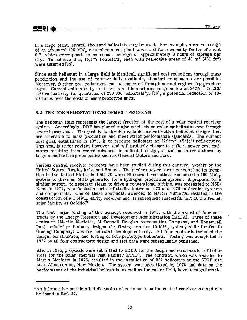
TR-459S=~I '.!: --011~~

In a large plant, several thousand heliostats may be used. For example, a recent designof an advanced lOO-MW central receiver plant was sized for a capacity factor of about0.7, which corresponds eto an annual average of approximately 8 hours of s~orage p~rday. To achieve this, 15,177 heliostats, each with reflective areas of 40 m (431 ft )were assumed [35].

Since each heliostat in a large field is identical, significant cost reductions through massproduction and the use of commercially available, standard components are possible.Moreover, further cost reductions can be expected through normal engineering ~evelop­

rnent. Current estimates by contractors and laboratories range as low as $42/rn ($3.90/ft 2) reflectivity for quantities of 250,000 heliostats/yr [36], a potential reduction of 10­20 times over the costs of early prototype units.

6.2 THE DOE HELIOSTAT DEVELOPMENT PROGRAM

The heliostat field represents the largest fraction of the cost of a solar central receiversystem. Accordingly, DOE has placed major emphasis on reducing heliostat cost throughseveral programs. The goal is to develop reliable cost-effective heliostat designs thatare amenable to mass production and meet strict performance s1fndards The currentcost goal, established in 1975, is to produce heliostats at $72/m ($7/ft~) reflectivity.This goal is under review, however, and will probably change to reflect newer cost esti­rna tes resulting from recent advances in heliostat design, as well as interest shown bylarge manufacturing companies such as General Motors and Ford.

Various central receiver concepts have been studied during this century, notably by theUnited States, Russia, Italy, and France. The modern power tower concept had its incep­tion in the United States in 1969-70 when Hildebrant and others conceived a 500-MWt hsystem to drive an MHD generator for a hydrogen production system. A proposal for asimilar system, to generate steam to drive a conventional turbine, was presented to NSF/Rand in 1972, who funded a series of studies between 1973 and 1975 to develop systemsand components. One of these contracts, awarded to Martin Marietta, resulted in theconstruction of a 1 MWtg cavity receiver and its subsequent successful test at the Frenchsolar facility at Odiello.

The first major funding of this concept occurred in 1975, with the award of four con­tracts by the Energy Research and Development Administration (ERDA). Three of thesecontracts (Martin Marietta, McDonnell Douglas Astronautics Company, and HoneywellInc.) included preliminary designs of a first-generation lO-MWe system, while the fourth(Boeing Company) was for heliostat development only. All four contracts included thedesign, construction, and testing of four prototype heliostats. Testing was completed in1977 by all four contractors; design and test data were subsequently published.

Also in 1975, proposals were submitted to ERDA for the design and construction of helio­stats for the Solar Thermal Test Facility (STTF). The contract, which was awarded toMartin Marietta in 1976, resulted in the installation of 222 heliostats at the STTF sitenear Albuquerque, New Mexico. The system was operational by 1978 and data on theperformance of the individual heliostats, as well as the entire field, have been gathered.

*An informative and detailed discussion of early work on the central receiver concept canbe found in Ref. 37.

33

TR-459S=~II.'----....--------------~~

Preliminary results also have been published [38]. Although the STTF was intended to bea research and test facility and the heliostats were designed to meet stricter perform­ance plans, considerable insight and experience into large-scale production was obtained.

The goals and approach of the heliostat development program are described in some de­tail in Ref. 39. Heliostat design has already progressed through several generations, asshown in Fig. 6-5, [41, p, 7] starting with the original National Science Foundation hello­stat and progressing to the prototype heliostat design. Additional paper/test hardwaregenerations are expected.

In 1977, a solicitation was released to design low-cost prototype heliostats. ERDAawarded contracts to McDonnell Douglas, General Electric, Boeing, and Solaramics. TheMcDonnell Douglas and Solaramics heliostat designs use glass mirrors and a steel struc­ture. The General Electric and Boeing designs involve less rigid, cheaper heliostat mir­rors encased in inflated plastic enclosures. The plastic enclosure designs result in bothlower mirror costs and lower reflectivity. One major cause of reflectivity loss is becauseof transmission losses through the plastic enclosure.

The McDonnell Douglas low-cost prototype design was selected as most promising at thebeginning of FY78. To foster competition, contracts were awarded to five separate con­tractors to build prototypes. All of these prototypes will use the glass-mirror design, be­cause the requisite plastics technology is not advanced enough to inspire confidence inthe plastic enclosure design. These low-cost prototypes are referred to as second­generation heliostats. While the glass-metal prototypes are constructed, research on de­velopment of suitable plastic materials for use in the enclosed heliostat design will becontinued.

While second-generation prototype heliostats are being built, work is proceeding on athird-generation design. Twelve special studies are being performed on heliostat com­ponent design and maintenance. A new heliostat components solicitation was released in1978. Resulting design improvements are planned to be incorporated into a third­generation heliostat design in the early part of FY81.

Two second-generation designs discussed here are those proposed by McDonnell DouglasAstronautics Company (MDAC) and General Electric (GE). They represent the two ge­neric heliostat concepts already described.

6.3 DESCRIPTIONS OF GENERIC HELIOSTAT DESIGNS

Two generic heliostat concepts are being studied by several contractors: the glass-steeland inflated plastic bubble concepts, now best represented by the designs of MDAC andGE, respectively. The following describes the design, manufacturing, and installation ofthese designs [3, 34].

6.3.1 The McDonnell Douglas Prototype Heliostat Design

The prototype heliostat design portrayed in Fig. 6-6 and Table 6-1 summarizes the tech­nical characteristics of this design. The heliostat is divided into four subassemblies.These subassemblies are the reflector panel (one-half of the reflective unit), the driveunit (including the pedestal), the foundation, and the heliostat electronics (including con­trollers and control sensors).

34

TR-459S=~I(.I-----------------------------

Table 6-1. TECHNICAL DESCRIPTION-COLLECTOR SUBSYSTEM

• Reflector-6 laminated reflector mirrors bondedto the reflector support structure.

• Reflec tive SurfaceReflective Surface AreaSecond Surface MirrorGlass Back Lite

• Mirror Backing StructureIMBD Cross Beam 14 GageOUTBD Cross Beam 18 GageDiagonal Beam 14 GageHats 16 Gage

• Drive-Consists of a rotary azimuth drive,a doublejack elevation drive, center main beam, and pedestal.

Center Main BeamTubeFlange

Elevation DriveJacks

Motor (Two)

Drag Link-Weldment

Azimuth DriveHousing-WeldmentDrive Unit (Retainer)Helicon InputHarmonic Output

Final Drive RatioMotor

Pedestal

Power Distribution Equipment and WiringStep Down Transformers

Position IndicatorsIncremental Encoder-Motor Tum Feedback

• Control/Instrumentation EquipmentData Distribution InterfaceDigital MicroprocessorCommunication Interface

Heliostat ControllerDigital MicroprocessorDrive Motor ControllerCantrol SensorsCommunication Interface

787 kg (1734 Ib)49.05 m2 (528 ft2)1.5 mm (0.060n)

4.8 mm (0.1875")

469 kg (1034 Ib)173"-27" deep173fT- l I fT deep112"-26" deep130"-6"

578 kg (1273 Ib)

122 Kg (268 lb)81 ' L 16" dia.18fT square

102 kg (225 Ib)5 ton ball screw (63kg, 139 Ib)

1/4 hp; 480 VAC (9.5kg., 21 Ib)

29.4 kg (65 Ib)

185 kg (407 Ib)108 kg (238 Ib)68 kg (150 lb)162:1242:1

39,204:11/2 hp; 480 VAC (8.6kg, 19 lb)169 kg {373 Ib

4160 VAC, 3- Phase480 VAC, 3-Phase

Hall effect sensors

1985 readiness78 per field of 25,000

1 per heliostat

37

TR-459S=~I~_I-------------------------

Table 6-1. TECHNICAL DESCRIPTION-COLLECTOR SUBSYSTEM (concluded)

Signal Distribution EquipmentFiber Optic Transmission Cable Included in power

cable

• FoundationConcreteSteel ReinforcementSteel Form

5478 kg (12076 Ib)194 kg (428 Ib)34 kg (75 Ib)

38

TR-459S=~I ;.;;-~ ~. ------------------------------.-;;~

Refleetoe, Each reflector panel is composed of six mirror modules and a support frame.The mirror modules (Fig. 6-7) [3] are 1.22 by 3.35 m (48 by 132 In.) and made of a 1.5 mm(0.060 in.) second surface mirror laminated to a 4.8 mm (0.1875 in.) glass back panel.The clean reflectivity is estimated to be from 0.92 to 0.95, depending on the thicknessand chemical state of the glass,

The mirror assembly support structure is shown in Fig. 6-8 [3]. Each of the laminated·mirror modules is stiffened with a pair of hat-section stringers which are part of the sup­port structure assembly and are bonded to the glass when the reflector is assembled.

The 12 hat-section stiffeners are attached to the two cross beams that run the long dis­tance of the reflector assembly, The deep, inboard cross beam is a 14-gage galvanizedsteel sheet, 0.476 m (18-3/4 in.) deep and 7.62 ern (3.0 In.) wide. The shallow outboardcross beam is IS-gage galvanized steel, 12.7 em (5.0 in.) deep and 5.72 em (2-1/4 In.)wide. This cross beam is attached to the main beam by diagonal frames (beams) whichtie into this cross beam at two points that are 4.62 m (167.9 in.) apart. These diagonalbeams are 6.35 em (2.5 in.) wide with 1.91 ern (3/4 in.) return flanges.

Drive Unit. The drive unit is composed of a rotary azimuth drive, a double screw jackelevation drive, and a pedestal. All drive motors are three-phase, 480-volt AC. Thefunction of the drive unit assembly is to rotate the heliostat mirror about the azimuthand elevation axes. The drive unit will be operated for solar tracking, emergencySlewing, stowage, and maintenance activities. Major performance requirements are de­scribed in Table 6-2.

The design life of the drive unit is 30 years. The drive unit is required to move the mir­ror from a stowed position to acquire the sun, track the sun during the day, and returnthe mirror to its stowed position at the end of the day. This lifetime is planned to beachieved without any scheduled maintenance activity.

The pedestal is a vertical tube 3.18 m (125 in.) high. At the top, the drive unit is weldedto the pedestal; at the bottom, the lower 1.12 m (44 in.) is expanded to give a slight taperfor slip-joint attachment to the rigid foundation.

The central torque tube main beam connects the two reflector panels (the reflectiveunit) together and ties the reflector to the elevation hinge and the elevating jacks at thetop of the drive unit assembly. The main beam carries all the airloads and dead weightloads from the reflector to the pedestal.

Heliostat Electronics. The heliostat controller is located in a housing on the top of thedrive unit. The controller receives and transmits commands from the collector con­troller and responds to requests for data. A microprocessor calculates the motor revolu­tions required to maintain tracking and activates the motor controllers. The motorcontrollers switch the motor on and off to produce the required motion. The motor revo­lution sensors detect motor revolution and direction, and the controller maintains a countof accumulated revolutions. A nonvolatile memory retains motor counts and alignmentdata in the event of a loss of power. The field wiring terminates at a junction box lo­cated on the pedestal. Data are routed to the heliostat controller, decoded, and relayedto the next heliostat in the link if not addressed to the receiving heliostat, Acknowledg­ment of receipt of a message and status are also transmitted.

39

TR-459S=~I '.1 ----------------------------

Table 6-2. DRIVE UNIT REQUmEMENTS

Requirement Azimuth Elevation

Travel + 2700 o to -1800

Maximum Travel Time Under Load 1800 in 15 minutes

Maximum Static Load 9830 N-m -32,650 N-m(87,000 in. Ib) -289,000 In.-Ib)

= 00

Maximum Starting Load 10,050 N-m + 13,890 N-m(89,00 in.-Ib) + 122,900 inv-lb)

= -50 0

Maximum Running Load 10,050 N-m + 26,790 N-m(89,000 inc-lb) + 237,100 inv-lb)

= -50 0

Maximum Overturning Moment 42,140 N-m(373,000 inv-lb)

Backlash/Hysteresis 1 mrad 1.6 mrad

Back Drive None None

Life 30 years 30 years

Minimum Stiffeners 1.13 x 196 N-m/rad 1.516 x 106 N-m/rad1.0 x 10 In.-lb/rad 1.342 x 107 in.-lb/ rad)

42

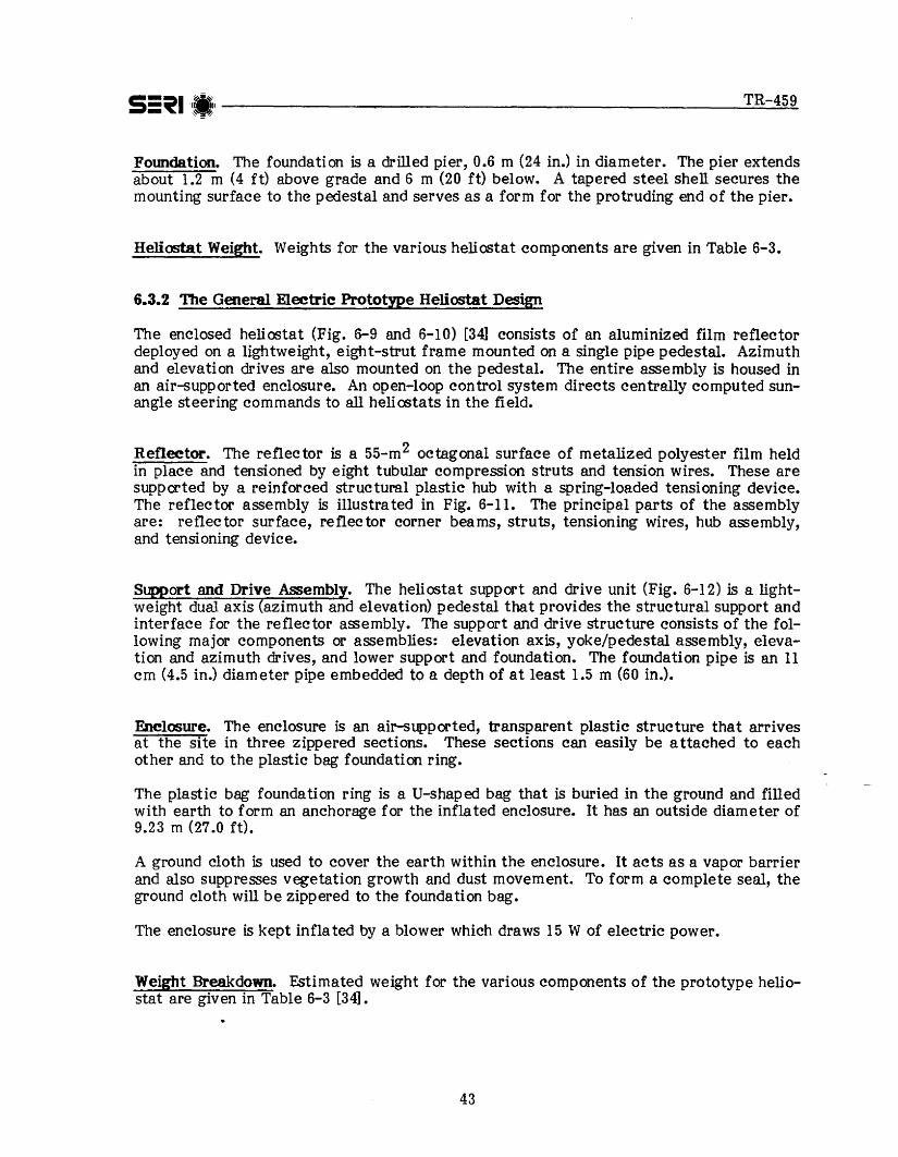
TR-459S=~I I.~ I --------.....--------------------..:::.=:~~-~ .•Foundation, The foundation is a drilled pier, 0.6 m (24 in.) in diameter. The pier extendsabout 1.2 m (4 f t) above grade and 6 m (20 f't) below. A tapered steel shell secures themounting surface to the pedestal and serves as a form for the protruding end of the pier.

Heliostat Weight. Weights for the various heliostat components are given in Table 6-3.

6.3.2 The General Electric Prototype Heliostat Design

The enclosed heliostat (Fig. 6-9 and 6-10) [34] consists of an aluminized film reflectordeployed on a lightweight, eight-strut frame mounted on a single pipe pedestal. Azimuthand elevation drives are also mounted on the pedestal. The entire assembly is housed inan air-supported enclosure. An open-loop control system directs centrally computed sun­angle steering commands to all heliostats in the field.

Reflector. The reflector is a 55-m2 octagonal surface of metalized polyester film heldin place and tensioned. by eight tubular compression struts and tension wires. These aresupported by a reinforced structural plastic hub with a spring-loaded tensioning device.The reflector assembly is illustrated in Fig. 6-11. The principal parts of the assemblyare: reflector surface, reflector corner beams, struts, tensioning wires, hub assembly,and tensioning device.

Support and Drive Assembly. The heliostat support and drive unit (Fig. 6-12) is a light­weight dual axis (azimuth and elevation) pedestal that provides the structural support andinterface for the reflector assembly. The support and drive structure consists of the fol­lowing major components or assemblies: elevation axis, yoke/pedestal assembly, eleva­tion and azimuth drives, and lower support and foundation. The foundation pipe is an 11ern (4.5 in.) diameter pipe embedded to a depth of at least 1.5 m (60 in.).

Enclosure. The enclosure is an air-supported, transparent plastic structure that arrivesat the site in three zippered sections. These sections can easily be attached to eachother and to the plastic bag foundation ring.

The plastic bag foundation ring is a V-shaped bag that is buried in the ground and filledwith earth to form an anchorage for the inflated enclosure. It has an outside diameter of9.23 m (27.0 ft),

A ground cloth is used to cover the earth within the enclosure. It acts as a vapor barrierand also suppresses vegetation growth and dust movement. To form a complete seal, theground cloth will be zippered to the foundation bag.

The enclosure is kept inflated by a blower which draws 15 W of electric power.

Weight Breakdown. Estimated weight for the various components of the prototype helio­stat are given in Table 6-3 [34].

43

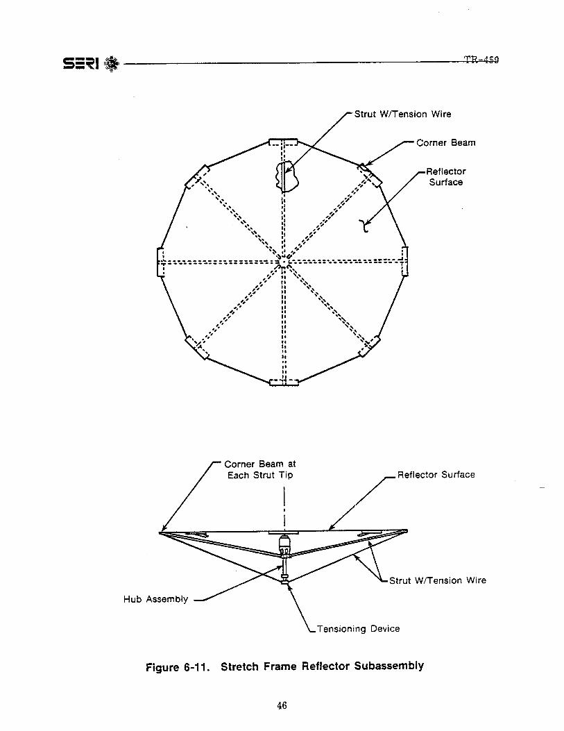
TR-459S=~I ,111------------------------"-=--:=

Table 6-3. GENERAL ELECTRIC HELIOSTAT WIDGHT BREAKDOWN

Assembly Weight, kg rn»Reflector

Support Structure and Driver

Controls

Enclosure

Foundation

Installation (Packaging)

31.3 (69)

16.3 (36)

14.5 (32)

166.0 (366)

76.2 (168)

6.8 (15)

6.4 KEY COST FACTORS IN HELIOSTAT DESIGN

A significant factor in all heliostat designs is the total allowable error allocation. Sys­tem performance is based upon a high percentage of reflected sunlight hitting the re­ceiver, and accumulated error from all sources affecting a heliostat is considered part ofthe total field efficiency. Errors occur either from wind- or gravity-induced deflectionsof the structure, mechanical failures in the various heliostat subassemblies, foundationmisalignment, thermal deformation of components such as mirror modules, and positionaluncertainties in the control and instrumentation system.

Design of the various subassemblies or components depends on compromises between costfactors and performance standards; the goal is to produce the lowest overall installedfield cost. A heliostat, therefore, has to meet requirements derived from total annualsystem performance requirements.

Certain factors affect particular elements of a heliostat. Table 6-4 identifies those de­sign parameters that significantly affect cost.

The highest costs in the "hard" (glass/steel) heliostat design involve the drive unit and thereflective unit. The drive unit must be able to withstand the full torque induced on thestructure by the highest winds encountered during operations or emergency stow condi­tions. These loads may exceed 30,000 N-m (289,000 in.-1b) at certain times; the drivemust be able to withstand these loads without permanent deformation or breakage.

In addition, the drive unit (which includes position indicators such as encoders) musttrack with great precision in order to assure that the reflected beam intercepts the re­ceiver. The allowable backlash on a typical drive mechanism is 1 mrad (3.3 arc-min) forazimuth and 1.6 mrad (5.3 arc-min) for elevation. This degree of backlash is more strin­gent than that usually encountered in commercial applications.

The glass mirror accounts for only a small fraction of the cost of the reflective unit.The majority of the cost lies in the assembly of individual mirror modules.

The third major cost element for a hard heliostat is the foundation and site preparation,which accounts for more than 20% of the total installed cost. The costs of the founda­tion are largely determined by the allowable error in heliostat alignment and deflections

48

TR-459S=~I I*,I ------------------------------­-~ ~

Table 6-4. DESIGN PARAMETERS AFFECTING HELIOSTAT ELEMENTAL COST

Component Significant Design Parameters

Structure

Drive Mechanisms

Elec tronic/Elee trical

Foundation

Installation and Assembly

Control

Reflective Surface

Reflective area, operation wind loads, error budget

Operational wind loads, slew speed, error budget

Operational modes, motor power, error budget

Site characteristics, error budget

Labor costs, adaptability to tooling

Operational and safety requirements, error budget

Spectral reflectivity, reflective area, wind loads,thermal deformation

and by soil characteristics at the site. Many desert soils contain large quantities ofmaterials like (e.g., or bentonite) that are subject to long-term shifting. Accordingly,they require more preparation and a larger foundation.

The foundation, in addition to supporting the weight of a heliostat, must be sufficientlystrong to withstand overturning by the wind without permanent deflection in either thepedestal or the soil. For the MDAC design, this overturning point may reach as high as42,140 N-m (373,000 in.-lb).

The elemental cost breakdown for the "soft" or plastic bubble enclosed heliostat isslightly different. Because of the protection afforded by the plastic enclosure, windloads are less; as a consequence, costs of the drive unit and reflective unit are less. Thefraction of cost attributed to the structure, however, increases because of the cost ofthe plastic enclosure. Foundation and site costs constitute a slightly higher proportion ofthe total cost than for a hard heliostat.

Critical areas for cost reductions can be identified for each generic design. For theglass/steel heliostats, major emphasis should be placed upon the drive units, the reflec­tive unit (including structure), foundations, and site development. The more equal distri­bution of costs in the enclosed bubble design dictate that all elements receive closer at­tention. Major emphasis should be placed upon the foundation, site preparation, and theheliostat structural support and protection.

49

50

TR-459S=~I·I.;1-------------------------~ ~.

SECTION 7.0

PROTOTYPE HELIOSTAT COST SCENARIOS*

7.1 INTRODUCTION

Establishing an adequately detailed costing scenario is the fundamental requirement forestimating and predicting cost reductions. This section presents the costing scenariosthrough description of the basic characteristics of market potential, production and in­stallation volume, and the general configuration of the manufacturing/assembly facilitymodule. This section also indicates the points in cumulative production volume where aneffective, steady-state production process may be established along with the associatedfirst-unit cost for the steady-state scenario.

The scenario presented in this section represents only one of many possible scenarios.Variations in market growth and location, competition, basic design, available productiontechnology and resources, and government and business policy may have a significant im­pact on the scenario and cost-reduction rate.

The term production here includes factory procurement, fabrication, assembly,andcheckout; transportation and handling required to ship the hardware to the installationsite; and field procurement, fabrication, assembly installation, and final checkout of thehardware.

7.2 FACTORS INFLUENCING COST SCENARIOS

In developing cost scenarios for a prototype heliostat, the following factors have beenconsidered: (1) market projections, (2) the implied growth of volume, (3) design and de­velopment status, (4) plant and equipment impacts, and (5) management alternatives andconcerns.

7.2.1 Market Potentials

The market for heliostats is tied to the cost and availability of alternate energy prod­ucts. The basic economic trade is the annual cost, including maintenance, per Btu of theincremental capital employed in collecting solar energy versus the annual cost per Btu ofalternative fuels and other energy sources. For some potential solar energy users, thisissue has been marked by considerable uncertainty about the future price of fuels and thecapital needed for solar applications. Some analysts believe that the market is generallyunfavorable for centralized solar systems, but concern about the future availability andcost of al ternative sources of energy and the intrigue of a free and renewable energysource keep interest high.

These circumstances have made it difficult to identify a broad market based on currenteconomic analysis, although the price trends of oil and gas and cost inefficiencies associ­ated with using coal or nuclear power for intermediate-sized plants certainly suggest amarket potential, especially with incentives. As a result, market forecasts have been

*This section was written with the assistance of J. H. Nourse of McDonnell DouglasAstronautics Company [41].

51

TR-459S=~I !;t.-~I ------------------------------ ~- ~

based on a penetration analysis given an absolute energy demand, expected growth in ser­vice by alternative energy sources, energy short-falls, and "target" solar energy costs.

Sandia Laboratories specified that Prototype Heliostat Study Contractors consider designand production scenarios that would be appropriate at rate production heliostat outputsof 25,000, 250,000, and 1 million units per year. In addition, a one-time pilot productionof 2,500 units was to be analyzed. Sandia also indicated that the design and productionscenario be conceived so that costs associated with the higher production rates are con­sistent with the DOE goal of $72/m 2 reflectivity. Other than stating that the marketcover eight Southwestern states in the 1990s, no other market description was indi­cated. Sandia's main purpose was to determine the costs that could be expected undercertain and steady market conditions.

It is, however, necessary only to characterize and shape the growth of the market in gen­eral for purposes of cost reduction analysis and technology readiness considerations.Figure 7-1 shows one possible market situation [3]. Although the details may be out­dated, they are representative of the general aspects of a market plan considered at thetime of the study. Both the total market and an assumed share for one producer are indi­cated, as well as a possible gap in 1985 between overall demand for energy and this parti­cular market scenario.

The illustration may be considered in phases. The first is a period of government­supported development projects requiring limited heliostat production capacity. At anygiven time, demand for an individual supplier's product may range from the total marketto none. Then, a period of transition is expected where eventual users may begin to de­ploy the concept on a limited basis provided that any economic disparities with competi­tive energy sources are balanced by incentives. This is perhaps the most critical periodto the survival of the concept, and costs must not exceed goals. Of course, the finalphase is the most unpredictable; it depends on the relative success of the intermediatephase, as well as on the cost and availability of alternative energy. It could be the periodin which both the technology and the relative cost of solar energy have received users'acceptance. If expectations about energy shortages prove true, the potential demand forand production of heliostats could be great.

7.2.2 Produetion Volume Progression

As indicated, the volume scenario established for the McDonnell Douglas PrototypeHeliostat Study [3] calls for 25,000 heliostats/yr at the lowest commercial rate. For thestudy, it was assumed that the baseline plant (25,000 units/yr) will initiate operations atthe 100,000th unit and continue production for 500,000 units over the next 20 years. Atthis period, production and installation capacity increases to 250,000 units/yr; an addi­tional 5 million units will be produced at this rate. After 15-18 years of operation inthese facilities, capacity increases to 1 million heliostats/yr and continues for another 20years.

This scenario provides three important variables-cumulative volume, annual rates ofproduction and installation, and rate of volume growth. While cumulative volume may bethe primary cost-reduction curve variable, quality and quantities of production andgrowth rates had a much more significant impact on the production and installation sce­narios devised for the Prototype Heliostat Study. The study assumes a steady productionrate where productive resources may be selected and geared in just the right balance toeconomically achieve required output over the expected production period.

52

TR-459S=~I.I ---------.,,.-----------------------The expected rate and quality of growth further influences the timing and degree of cap­ital employment. Capacity growth, although potentially rapid in the first 5-10 years, isexpected to be intermittent following the nature of demand. This could delay installa­tion of the baseline rate production facilities, or cause it to be staggered until a steady25,000-unit/yr output appears maintainable•. As indicated, growth in capacity from thispoint has been portrayed in the study as a series of 20-yr steps extending approximately50-60 years to about the year 2045. If this is true it could lead to a somewhat slackenedrate of innovation and the actual growth will probably occur in more frequent steps witha modular approach to capacity expansion.

7.2.3 Design and Development Status

The status of design, development, test, and evaluation (DDT&E) is of interest from anumber of perspectives. The issue is not just whether a design is proven, but alsowhether it is producible and cost effective, will have future technological impact, andthe extent to which the innovation may be implemented within current schedules or mustbe programmed into the future. From a cost reduction viewpoint, very little improve­ment occurs in actual hardware cost while the design is still in a state of change. How­ever, parallel design-to-cost studies may identify and project "paper" improvementsleading to rapid cost reductions as advance design-to-cost configurations and plans canbe incorporated.

The baseline 25,000/yr scenario represents plans for a well conceived, advanced design,although the production plans for early supply assume that many specific design or pro­duction innovations will not be immediately available for technological or economicreasons. Heliostat design has already progressed through several generations, as shown inFig. 6-5, starting with the original National Science Foundation heliostat and progressingas far as the prototype heliostat design. Additional paper/test hardware generations areexpected.

A considerable amount of heliostat development effort will have been expended in re­search experiments such as the Barstow plant, and in second-generation, preproductionhardware. Also, there will be some final production design involved in the first prototypepilot production purchase. However, once the design has been established, further designeffort is self-supporting; Le., only design changes that will result in net design/hardwarecost reductions will be incorporated.

7.2.4 Plant and Equipment Impact

A fourth major consideration is the impact of prudent use of plants and equipment.Figure 7-2 shows the importance of finding the right combination. The figure indicatesthe approximate break-even investment associated with a savings, using an existingmethod, of 1 person-minute on each heliostat produced, transported, and installed in a20-yr period, at various annual production rates. In the example, any investment thatcosts less than $264 thousand would result in a savings at a production rate of 30,000heliostats/yr. Given this incentive, the objective is to identify cost-saving equipment!processes and plant arrangements; influence the design to permit desirable alternatives;and balance the use of plant and equipment resources with respect to desired output andother management considerations.

54

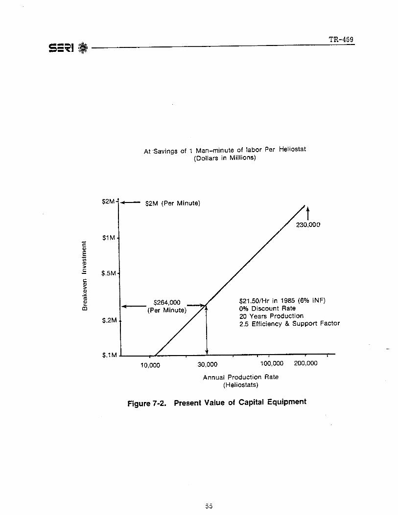
TR-459S=~I.!-----------------------7.2.5 Management Altematives and Concern

Management concerns generally relate to a specific firm's policy, traditions, practices,and fiscal constraints. They affect decisions about market approach, resource sharing,allocation and balance, make-or-buy resolutions, organizational structure, labor andother industrial relations, and choice of technology. The firm must also consider avail­ability of funds, labor, and other resources; the impact of outside influences such as gov­ernment, unions, and special interest groups; the flexibility of their business approachand the technical requirements/acceptability of their product in the face of market char­acteristics and competition; and finally, the acceptable risk exposure and return on in­vestment. The result of these considerations sets the ultimate course of the productionscenario and the overall business approach in a manner intended to assure the firm's fi­nancial success and meet market requirements.

7.3 DESCRIPTIONS OF THE BASELINE PRODUCTION SCENARIO

The baseline production scenario for the MDAC and GE heliostat design describes pro­duction at a rate of 25,000 units/yr. Thus, the 25,000 units/yr rate has been studied ingreater depth than other production rates. This rate represents significant high-volumeproduction situations, yet may be easily translated into higher or lower production-ratescenarios. As a result, this scenario effects a viable business approach that meets earlybusiness constraints and simultaneously attempts to capture an important share of futuremarkets. A summary of the baseline production scenario and changes in the scenario forhigher production rates for each of the heliostat designs follow [3,34]. More detailed dis­cussion of the production concepts is found in the cited references. Additional informa­tion on high-production heliostat manufacture can be found in Ref. 1.

7.3.1 The McDonnell DOuglas Prototype Heliostat Design Production Scenario

In developing the baseline production scenario for MDAC prototype heliostat design, theoverall approach has been to minimize hand labor and achieve quality through mechani­zation, with as much flexibility and as little risk as possible.

Equipment has been designed to reduce hand labor and to assure continuously acceptableproduction performance. Wherever practical, automatic handling equipment has beenused to keep operator handling time to a minimum, especially where operation cycles in­volve manual loading or unloading. Reflective unit equipment used for fabrication,transfer, and installation has been mechanized to address special problems in handlingglass and to minimize potential damage.

Assemblies are automatically checked out with special equipment in the factory to re­duce field problems. Pre-assembled units are installed with equipment designed to cor­relate time, crew size, and proficiency with equipment capabilities rather than humancapabilities, and final alignment and checkout is largely automated. Thus tools andequipment are designed mainly for automatic production, according to specifications andto production rates.

56

TR-459S=~I'*I:---------.--------------------­- '.

7.3.1.2 Quality Assurance

The quality assurance approach calls for verification of hardware through control of in­coming parts and materials and attention to the quality of tooling and equipment. Thequality of incoming materials and parts is controlled through careful supplier selectionand source inspections for critical items. Inspection at the Receiving phase is carriedout for identification, certification, and any damage. Tooling and equipment are de­signed within specified tolerances; an automatic "out of spec" trend warning triggers thenecessary tool adjustments. Automated end-item inspections and alignments are used forthe reflector panels and at checkout stations for the pedestal/drive/electronics unit andpower distribution modules. A special test van is used in conjunction with digital imageradiometers and master control support to automatically check and align an installedheliostat.

7.3.1.3 Transportation to Installation Site

Transportation covers the transportation of final assemblies to sites, and delivery of in­stallation equipment. In addition to the foundation and field wiring materials, only threeend-products must be delivered-reflector panels, drive/pedestal/electronics units, andpower distribution modules. Special reusable open containers are designed for ease ofaccess and handling. Placement and removal will be automatic for these containers,using robot-like controls. Equipment is transported from factory to site by a manu­facturer-owned truck fleet.

7.3.1.4 Installation Equipment Ownership

Another important provision in the overall approach is that the heliostat manufacturerwill control (through ownership or sale/leaseback) the special equipment used to trans­port, install, and check the heliostats. The manufacturer will provide the equipment toeach installation on a cost-sharing basis, and assure that an efficient, uniform plan isavailable to any installation. This equipment is important to the installation scenario atall volume levels and probably should be made available as early as the pilot production.

7.3.1.5 F1exib~ty

Flexibility has been considered in both macro- and micro-modularity characteristics ofthe facility. The plant may be thought of as a production module that may be more thantripled in capacity by adding shifts, extending the work week, or adding automationequipment simultaneously in a few critical areas. When production capacity is reached,or design technology and competition dictate, anew, upgraded module may be added inthe most desirable location. Assemblies such as the drive, electronics, and panels mayalso be moved into their own facilities. Fairly low production rates, at a greater cost perunit, may be accommodated by eliminating a shift, deferring purchase of certain equip­ment, or by increased use of the industrial base. In effect, the scenario permits a logicalextension of pilot facilities.

Such flexibility allows a manufacturer to take some financial risk in proportion to prod­uct demand and at the same time remain reasonably current in production and designtechnology. In addition, use of the industrial base for production of tubes and beams,glass, chips, drives, and other components reduces capital equipment requirements. This

57

TR-459S=~I '.!----~------------

approach permits a firm to expand according to market conditions, available resources,product acceptability, and profitability.

1.3.1.6 Make Or Buy Plan

The make-or-buy plan is shown in Table 7-1, and indicates whether finished parts andmaterials are made in the heliostat production facility or are procured from outsidesources. Generally, if an item is commercially available from several sources, and ac­quisition of specialized capability is required, purchase of the items is likely. Makeitems, typically, are specially designed and are critical to schedule, cost, or process. Ob­viously, this plan is a fundamental variable in sizing a facility.

7.3.1.7 The Heliostat Factory

Figure 7-3 provides a schematic of the prototype heliostat production plant. The plant is62,500 ft2, located in the Southwest, and has access to rail lines and adequate roads. Thelocality also provides a work force of less than 300 predominantly unskilled factory em­ployees. The level of workers' skills permits low average labor wages, while the factoryburden and direct support typically reflect an operating stand-alone plant limited to oneproduct line. Annually, the factory produces 50,000 reflector panels, 25,000 drivelpedestal/electronic assemblies, and 25,000 foundation caps. The plant operates on a two­shift basis, 5 days per week, 240 days a year.

Reflector Panel

Figure 7-4 provides a pictorial schematic of the reflector panel fabrication and assemblyline. A total of 52 assemblers, handlers, and operators are required to run this line asfollows:

Hardware ElementMirror ModulesSupport StructureAssemble and Bond

Total

Workers16181852

The two glass lites are stacked on a reusable A-frame, and automatically loaded on con­veyors using vacuum cups. From that point, the mirror modules are fabricated, treatedwith adhesive, and lined up on the bonding tables. Each of the facets on the bondingtables is curved and canted individually so that each mirror module will rest in its appro­priate position relative to the other five modules.

The beams and hat sections for the support structures are delivered from the rolling mill,formed, and palletized for assembly. The details are purchased, formed, and palletized,and then delivered to the fabrication area after inspection. The inboard, outboard, anddiagonal beams are loaded into separate punch presses that automatically punch the boltholes. The parts then proceed on an overboard monorail to a weld and drill station wherethey are lowered into a floor-mounted fixture and secured. Spot welding of the inboardand outboard areas is accomplished simultaneously. After welding, the bolt holes for at­tachment to the drive units are jig-bored.

58

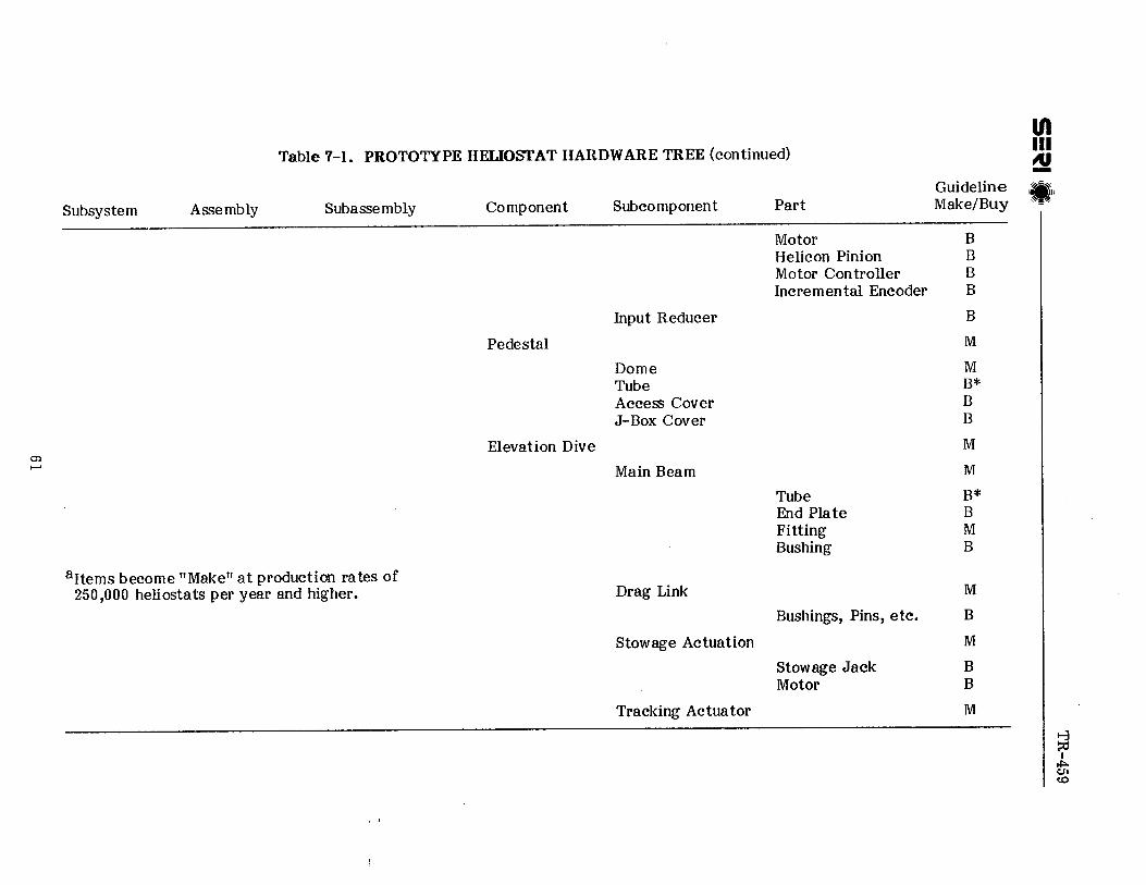
TR-459S=~I :;.1------~-------------------The welded structure is removed from the weld fixture and proceeds on a monorail totwo stringer attach stations. The 12 stringers are loaded and clamped in position in theassembly fixture, and the welded structure is lowered onto the stringers, clamped inplace, and bolted.

The structure is then removed from the tool and is moved by monorail to a dip-clean,rinse, and air-dry station prior to bonding the structure to the mirror modules. At thispoint, the structure is lifted from an adjacent conveyor by a fixture that places thestructure so that the hat sections rest on the two bond material lines that have beenappli ed to each mirror module. The fixture holds the drive unit interface in correctalignment with respect to the mirror module surfaces. The mirror module curve andcant, and the hat section interface imperfections, are taken up in the thickness of thebond line.

The reflector panel is ambient-curved and vacuum-lifted from the assembly line andplaced on shipping racks for transfer to the site. Special exhaust systems will removevapors emitted by the acids, solvents, and adhesives. The exhaust systems may requirescrubbers before the exhaust is released to the outside environment.

Special attention has been given to glass handling and transfer through the productionlines. Glass handling equipment will be completely automatic and include unstaeking ma­chines for removing large sheets of glass from vertical storage and placing them on ahorizontal production-line conveyor. Air float tables are used for transfer. Additionalhandling equipment includes a 90° conveyaized transfer unit.

Drive and Pedestal Fabrication and 1\$embly. Drive and pedestal fabrication and assem­bly comprises a series of relatively standard equipment lines for metal forming, joining,removal, and assembly that utilize automatic feed and clear features and are intercon­nected by conveyors, hoists, drive assembly carriers, and other handling devices. For ex­ample, shuttle-type loaders allow machining while hardware is being loaded and unloadedon the numerical control machining centers and vertical turret lathes. This also allowsindividual operators to service more than one machining activity. Automatic positionersand gravity-fed conveyors allow the large, bulky items like the main beam and pedestalto ron to their next station rather than be handled between stations. Where items re­quired several positions for assembly, such as on the azimuth drive, specialized equip­ment permits multiple part orientation by individual operators. The type of handlingequipment and tooling used reduces the cost of major machine tool investment. Figure7-5 shows the drive assembly flow and lists possible purchased materials and parts. Thebasic equipment required is:

Major EqUipmentNumber

Required

Flame cutterG&L vertical turret latheNumerical control latheAutomatic latheHydrosize machinePunch press line with coil straightHydraulic press (300-ton)Deep draw pres;Small pressMulti-drill stationNumerical control milling machine center K&T

2221112I1

~

67

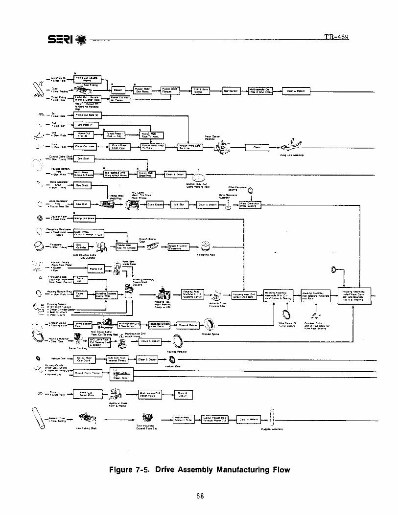
TR-459S=~II" ------------------------

Major EquipmentNumber

Required

Conventional millFusion welderInertia welderMarvel sawBroachAutomatic clean deburr stationCam grinder

Total

1622111

36

Minor Equipment

Material handling (conveyors, hoists) 106.68 m(350 ft)

Motorized drive carrier 5

In addition, an assembly and checkout station is required, as shown in Fig. 7-6, for inte­gration of the drives, electronics and pedestal.

Ninety-eight "B" welders, machinists, handlers, assemblers, and operators are required asfollows:

-Nurnber

Numerical Control MachinistsGeneral Machinists"B" WeldersProcess Machine OperatorsAssemblersHandlers

Total

837174

161698

Twelve of the above workers are allocated to the pedestal and foundation cap and 16workers to the azimuth drive assembly and final integration of the drivers, pedestal andelectronics. The remaining 70 workers are involved in fabrication.

Elec1ronics and Elec1rical Components. The electronic and electrical components-theheliostat controllers, data distribution interface (DDI), and pedestal junction box(J-box)-are listed as buy items. However, for costing purposes, the harness assemblieswill be made in-plant. Figures 7-7, 7-8, and 7-9 indicate the purchased parts, the manu­facturing flow, and processes involved in production of the heliostat controller, data dis­tribution interface, and harnesses. These flows are representative of the flows involvedwith the motor controller and encoder which are also buy items. The electronic assem­blies will be procured from sources that have programmable automatic sequencer and in­sertion equipment. The flow solder technique is employed to complete the circuits, and afunctional test and burn-in is accomplished prior to installation in the housing. Commer­cial-grade components produced to military specifications will be employed.

70

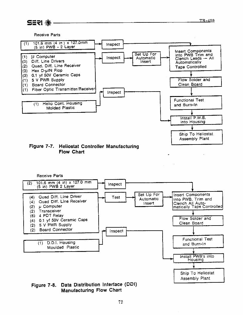
TR-459S=~II_ ---------------- _A total of 32 assemblers, technicians, handlers, opera tors, inspectors, electricians andmechanics are required, as follows:

Element Workers

Controller and DDIMotor controller and encoderHarnessMotor Test

Total

12992

32

7.3.1.8 Installation

The heliostat is assembled in the field from basic component subassemblies that havebeen checked in the factory. This simplifies field operations by reducing the number andcomplexity of tasks performed in the field. The installation is mainly achieved by tradelabor supplemented with specially trained operators and technical personnel. The laborforce is supervised by the heliostat manufacturer. Figure 7-10 provides the sequence ofinstallation events; time and resource requirements for one crew are shown in Table 7-2.

Foundation. Standard construction techniques are employed for foundation installation,and a number of methods could be employed. For the baseline method, rebar cages arefabricated in a site-located shop with the foundation cap welded to the top. At the sametime, pier holes are drilled using a high-powered auger. The completed cages are truckedto location and placed in the hole with light lifting equipment such that the cap extendsabove grade. Concrete obtained from a local batch plant and trucked to the area ispumped and vibrated through the top of the cap, filling both the hole and the cap exten­sion.

Labor is required as follows:

ElementWorkers

Crew Total

Cage FabricationSurvey and AugerInstallation

Total

78

1429

354070

145

These 145 workers are capable of installing 25,000 foundations in 25 weeks, including losttime for start-up/shutdown, personal time, fatigue shortages, inclement weather, andlost efficiency. However, the numbers shown exclude concrete truck drivers and batchplant laborers, who are covered in the concrete price.

Reflector and Drive/Control Unit. The reflector panels and drive/control units are in­stalled using the equipment depicted in Fig. 7-11 and 7-12. The drive/control installationequipment is used to lift the unit from the flatbed trailer, rotate it to a vertical position,and place the pedestal section over the tapered foundation cap. The drive unit is thenoriented to true north, and downward pressure and vibration are applied to seat the uniton the foundation. Once this is completed, the drive is filled with oil.

74

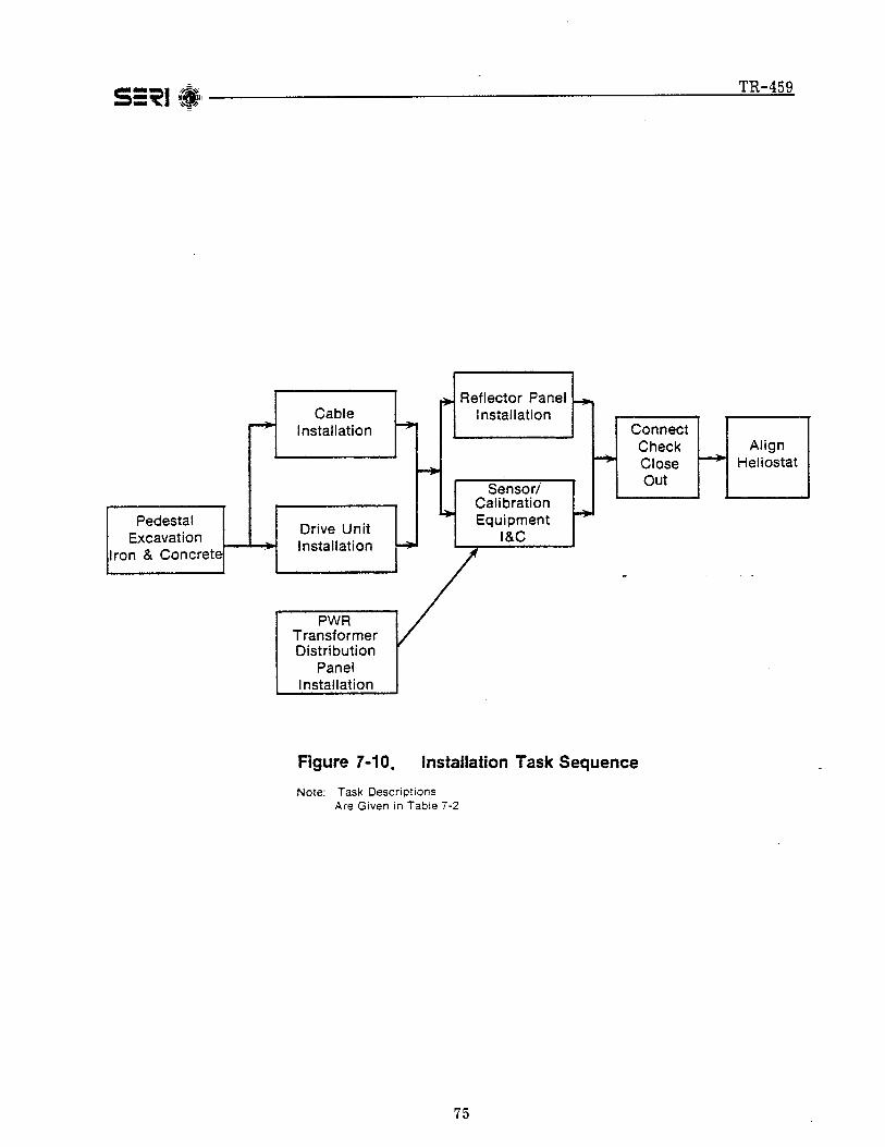
TR-459S=~I~" -----------------------=.::=--==-

Table 7-2. INSTALLATION TASKS AND CREW SIZE

Task Number Time/Heliostat Crew and Equipment Allocations

1. Pedestal Excavation 30 min/heliostat 4 TrucksIron Work and Concrete 2 Hydraulic Cranes

1 Auger Rigs3 Equipment Opera tors4 Truck Drivers2 Surveyors (part-time)2 Oilers2 Iron Workers4 Rodmen

12 Laborers

2. Cable Installation 18 min/heliostat 1 Cable Plow1 Cable Plow Operator2 Laborers

3. Drive Unit Installation 18 min/heliostat 1 Pedestal/Drive AssemblyInstallation Equipment

1 Installation EquipmentOperator

1 Millright1 Laborer

4. Power Transformer/ 90 min/312 helio- 1 MilfwrightDistribution Panel stats 2 LaborersInstallation 1 Truck

1 Forklift1 Truck Driver

5. Reflector Panel 21 min/heliostat 1 Reflector Panel AssemblyInstallation Installation Equipment

1 Installation EquipmentOperator

2 Hi-Lift Forklifts2 Forklift Operators2 Millwrights2 Laborers

6. Sensor/Calibration 8 hrs/3,000 heliostats 1 Field EngineerEquipment I&C 1 Electrician

1 Volt-Ohm Meter1 Oscilloscope

7. Connect, Check and 15 min/heliostat 1 ElectricianClose Out 1 Laborer

1 Test Set

8. Align Heliosta t 10 min/heliostat 1 Field Engineer2 Technicians1 Mobile Field Test

Station

76

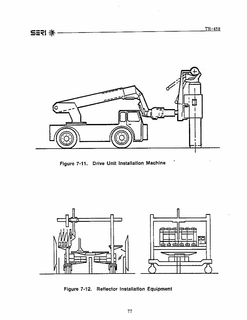
TR-459S=~I~'i ----------------------------

The reflector installation equipment is designed to simultaneously position two panelsnext to the drive unit and provide convenient access for bolting the panels to the driveunit. First, one pallet containing four reflector panels is loaded on each side of the in­stallation equipment using a high-lift forklift. The equipment is then driven over thedrive, and a manipulator arm on each side (only one is shown in the drawing) engages apanel. The arms move the panel to positions where they may be connected to the driveusing 8 bolts for each panel. The equipment is disengaged and moved over the next drive.

The work force employed is:

ElementWorkers

Crew Total

Drive/ControlReflector Panels

Total

36

9"

153045

These crews are sufficient to install 25,000 reflector and drive/control units in 39 weeks,with allowances for lost time.

Power Distribution and Sensor/Calibration Units. Installation of these elements includesburying 88,350 m of branch circuit cable and placing and checking 79 power distributionmodules and 8 digital image radiometers. The cable is "plowed in" using a standard cableplow that slices a V-groove in the soil to a .61-m depth and feeds cable into the bottomof the groove at a rate of 76 m/hr, As the cable is placed, the plow guides the soil backinto the groove. At each point where power is required or distributed, the plow stops anda large loop is allowed to form in the cable before the plow moves on.

Installation of the power distribution modules is basically a rnatter of pouring a smallfoundation at each position and setting the equipment. A field engineer must further in­spect the 8 digital image radiometers using a volt-ohm meter and an oscilloscope in thefinal alignment of the heliostats.

Labor is employed for these tasks as follows:

ElementWorkers

Crew Total

Lay CablePower Distribution ModulesDigital Image RadiometerConnect, Check, and Closeout

Total

3422

N/A

9428

23

Plowing in the cable and the connections requires 39 weeks. Only 3 weeks are requiredfor the power distribution modules and a little over I week is required to install the digi­tal image radiometers.

Alignment and Cheekout. A final tracking alignment and checkout are accomplishedusing a control van, the digital image radiometer, and the plant master control. Nomechanical adjustments are required for the heliostat after installation. The alignment

78

TR-459S=~I('! --------------------------

is done by establishing and adjusting position relationships in the heliostat controller toreflect the differences between the programmed placement of the heliostat and theactual position of the unit. New position information is required on the first alignment,and a subsequent alignment compensates for vertical errors.

The control van is connected into the data distribution interface once for 24 heliostats asthe heliostats read positioning information from a common optical data bus. The groupof heliostats is then activated, moved to standby positions, and established on track. Atthis point, the activities of the alignment branch into two categories: interacting man­machine alignment in the northern half of the field, and automatic search in the southernhalf.

In the interacting alignment, a sighting mirror is placed on the reflector edge, and the in­staller views the position of the image with respect to an alignment target on thetower. A verbal command is then given to the alignment operator in the control van thatbrings the spot on the target. Once the spot is on target, the digital image radiometer isused to establish the exact position and provide updated position information.

An automatic search technique will be used in the southern portion of the field becausethe heliostats will be in a nearly horizontal position during much of the day. It is there­fore inconvenient to attach a sighting mirror and observe the solar image. In the auto­matic search, the heliostat is moved in an expanding spiral search pattern until the tar­get is intercepted. Afterward, the digital image radiometer is used to set the exact posi­tion and update it as in the interacting technique.

In conjunction with these activities, the heliostat will be checked for tracking, a .satis­factory image quality, correct data and power transmission, and lack of lubrication leaksor installation damages. The labor required for this task is three 3-person crews over a39-week period.

7.3.1.9 Changes in the Scenario for Higher Production Rates

Three main changes have been made in the 250,000 heliostats/yr costing scenario. First,material weights have been reduced to their theoretical minimum for the mirror backingstructure and integrated drive unit structure. Second, parts have been eliminated in thedrive housing by assuming a welded flexspine/housing assembly. Third, automated assem­bly equipment has been deemed capable of eliminating 90% of hand labor and its addi­tional use is assumed. However, production plant adjustments necessary to assimilateau tomation assume that a lot of direct labor support is still required to maintain and pro­vide basic direction to the automated equipment. Two types of industrial "robots" wereconsidered: one produced by Unimation, Inc., which is used in numerous automobile pro­duction situations, and a highly flexible one produced by Cincinnati Milacron. These ma­chines are capable of performing almost any assembly, machine loading, welding, or han­dling operation. One other change assumed is that foundation installation will becomemore mechanized. Also, overhead is assumed constant (i.e., reduced fringe costs will bebalanced by increased equipment cost and fringe rates), so that overhead rates increase,dramatically. Additional changes, such as improved line flow, integration, and increasedsupplier control, are considered through the operation of the cost reduction curve.

The 1 million units/yr scenario assumes further that production facilities will be morefunctionally specialized; that designs, materials, and processes will continue to improve;and that greater control over supply will be achieved. It also may become feasible to

79

TR-459S=~II.'-----------------

vertically integrate the production of certain basic materials. All such changes havebeen given effect through adjustments along the cost reduction curve to reflect costs atthe 15 millionth unit.

7.3.1.10 Produetion Volume Impact on Average Unit Cost

The MDAC heliostat cost comparison is presented in Table 7-3. Figures 7-13, 7-14 and7-15 describe cost elements of the MDAC heliostat based on production rates.

The design/production, installation, and operating plans derived for the 25,000 units/yrscenario support the belief that the DOE goal of $72/m 2 reflectivity is obtainable. Forthe rate of 25,000 units/yr. the average unit cost is projected to be about 20% lower thanthat projected for the initial pilot production. Large cost reductions are projected for allelements except foundation and site preparation. However, the costly foundation pro­posed for this design/production scenario permits important cost reductions in otherareas by (1) supporting a larger heliostat, and (2) contributing to a simplified field assem­bly and checkout procedure. Perhaps the largest cost reduction is projected in the driveunit, which has been simplified in such areas as the housing, bearings, jackscrews, andvarious azimuth components. In general, projected cost reductions are associated withthe introduction of automated assembly and material transfer; numerically controlledmachines; automatic electronic component insertion; and wave soldering.

The average unit cost for a 250,OOO/yr production rate shows a significant reductioncompared with its estimated value at the 25,000 heliostats/yr rate. This cost reductionis supported by:

• Reduction of the material weights to their theoretical minimum for the mirrorbacking structure and integrated drive unit structure.

• Elimination of the parts in the drive housing by assuming a welded flexspine/housing assembly.

• Introduction of automation (industrial robots) capable of eliminating 90% of handlabor positions.

• Mechanization of the foundation installation.

• Improved line flow, integration, and increased supplier control.

The average unit cost reduction for the 1 million/yr production rate is not as significantas for the 250,000 units/yr scenario. It is assumed that further cost reductions will becaused by continued improvement of the design, materials, and processes; further func­tional specialization of the production facilities; greater control over supply; and verticalintegration of the production of certain basic materials.

7.3.2 The General Eleetric Prototype Heliostat Design Production Scenario

This subsection briefly summarizes the facilities, equipment, tooling, manpower, newmaterials, materials handling, quality control, and cost requirements needed to produce2,500 heliostats as a one-time purchase, and steady-state production levels needed for25,000, 250,000 and 1 million heliostats/yr. Detailed information on the manufacturingdesign for this heliostat is in Ref. 34.

80

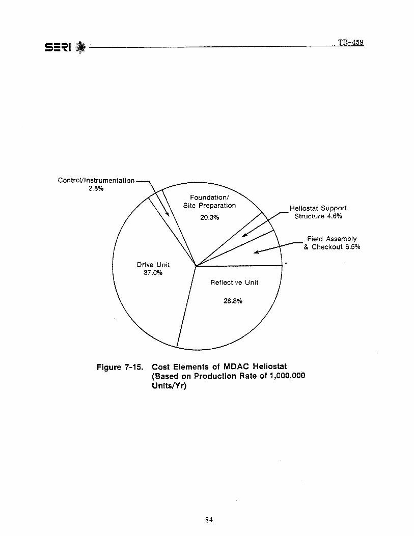
TR-459S=~II.I -------------------------------

The 25,000 units/yr rate has been applied to develop a baseline production scenario forthe GE prototype heliostat design. The overall approach for developing a costing sce­nario is similar to that applied for the MDAC prototype design.

Tables 7-4, 7-5, and 7-6 illustrate the production volume progression on the average unitcost while Fig. 7-16, 7-17, and 7-18 portray the relative changes in structural cost com­ponents of the GE heliostat based on production rates under consideration here.

7.3.2.1 Baseline Produetion Concept for 25,000 Heliostats/Yr

The facility concept f02the production of 25,000 heliostats/yr is shown in Fig. 7-19. Theplant occupies 3,700 m (39,812 ft2) and is operated on a 5-day, 2-shift basis using 43 di­rect labor personnel. The degree of automation is low.

The aver~ge unit cost for an annual production rate of 25,000 is estimated to be$81.09/m reflectivity, a decrease in cost of nearly 55%. Cost improvements range from40-65% over those of the pilot 2,500. Major improvements in the cost of the reflectiveunit, and field assembly and checkout, resulted in decreases of 57% and 63%, respec­tively.

7.3.2.2 Production Concepts for 250,000 and 1,000,000 Heliostats/Yr

Tables 7-4 and 7-5 illustrate some effects of increased production rates, plant character­istics, and heliostat cost. As higher levels of production are reached, the degree of bothautomation and vertlcal integration increases sharply. The manufacturing facility for250,000 heliostats/yr is presented in Fig. 7-20.

Production of 250,000 heliostats/yr necessitates a highly automated facility, divided be­tween two buildings to accommodate expansion. There are 151 direct labor personnel inthis plant, representing 1,656 heliostats per person, compared with 581 heliostats perperson at a 25,000/yr production output. At that level of production, an additional 279people would be required if the automation level remained the same as for a 25,000heliostat/yr production. However, automation could be greatly increased for 250,000units/yr.

The 250,000/yr capacity of this facility would be limited only by the areas available fordie casting, final assembly, reflector fabrication, and ground cloth fabrication. Throughthe addition of overtime and/or a limited third shift in these areas, the plant outputcould be increased to 300,000 heliostats/yr without affecting other areas or operations.

For an increase in production from225,000

to 250,000 units/yr. the average unit cost de­creased another 44%, to $45.39/m reflectivity, primarily because of automation. Thereflective unit and the heliostat support and protection subsystem showed the best costimprovements, Le., decreases of 58% and 74%, respectively. The drive unit showed a37% decrease. The remaining major elements showed cost improvement of 25% to 33%.

The GEl ,000,000 units/yr production facility consists of multiples of the 250,000heliostats/yr plant with an appropriate adjustment in film making capability. Two fulllines of film machinery would be required as well as additional materials handlingequipment.

85

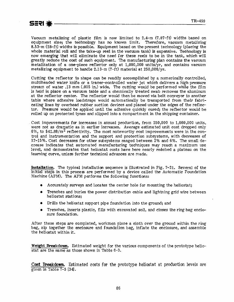
TR-459S=~I.'------------------------Vacuum metalizing of plastic film is now limited to 2.4-m (7.87-ft) widths based onequipment size; the technology has no known limit. Therefore, vacuum metalizing8.53-m (28-ft) widths is possible. Equipment based on the present technology (placing thewhole material roll and the take-up reel in the vacuum tank) is expensive. Technology isnow emerging that will eliminate the need for these reels to be in the tank, which willgreatly reduce the cost of such equipment. The manufacturing plan contains the vacuummetalization of a one-piece reflector only at 1,000,000 units/yr, and contains vacuummetalizing equipment to handle 2.l3-m (7-ft) material at 250,000/yr.

Cutting the reflector to shape can be readily accomplished by a numerically controlled,multiheaded water knife or a tracer-controlled water jet which delivers a high pressurestream of water .13 mm (.005 in.) wide. The cutting would be performed while the filmis held in place on a vacuum table and a chemically treated swab removes the aluminumat the reflector center. The reflector would then be moved via belt conveyor to anothertable where adhesive loadstraps would automatically be transported from their fabri­cating lines by overhead rubber suction devices and placed under the edges of the reflec­tor. Pressure would be applied until the adhesive quickly cured; the reflector would berolled up on protected tynes and slipped into a compartment in the shipping container.

Cost improvements for increases in annual production, from 250,000 to 1,000,000 units,were not as dramatic as in earlier increases. Average estimated unit cost dropped only6%, to $42.88/m2 reflectivity. The most noteworthy cost improvements were in the con­trol and instrumentation and the support and protection subsystems, with decreases of12-15%. Cost decreases for other subsystems ranged between 2% and 6%. The small de­crease indicates that automated manufacturing techniques may reach a maximum uselevel, and demonstrates that heliostat costs have here nearly reached a plateau on thelearning curve, unless further technical advances are made.

Installation. The typical installation sequence is illustrated in Fig. 7-21. Several of theinitial steps in this process are performed by a device called the Automatic FoundationMachine (AFM). The AFM performs the following functions:

• Accurately surveys and locates the center hole for mounting the heliostat;

• Trenches and buries the power distribution cable and lightning grid wire betweenheliostat stations;

• Drills the heliostat support pipe foundation into the ground; and

• Trenches, inserts plastic, fills with excavated soil, and closes the ring bag enclo­sure foundation.

After these steps are completed, workmen place a cloth over the ground within the ringbag, zip together the enclosure and foundation bag, inflate the enclosure, and assemblethe heliostat within it.

Weight Breakdown. Estimated weight for the various components of the prototype helio­stat are the same as those shown in Table 6-3.

Cost Breakdown. Estimated costs for the prototype heliostat at production levels aregiven in Table 7-5 [34].

86

TR-459S=~I;_'-----------------

Table 1-5. PROJECTED COSTS FOR GE HELIOSTAT DESIGN (1978$)

Installed Equipment Operation and Heliostat HeliostatProduction Investment Costs Maintenanc;e Installed Co~t

Level (in thousands of dollars) Costs $/m'" Cost $/m -R

1,000,000 171,619 26.77 $1,363 42.88250,000 64,254 27.24 $1,443 45.3925,000 13,351 50.48 $2,597 81.092,500 1,264 79.73 $5,686 178.83

1.4 STEADY-sTATE PRODUCTION VOLUME AND COST VARIATION

Although the information presented in previous sections provides an accurate summary ofthe design and baseline production scenario for each of the heliostat designs, it should berecognized that it represents only one of many possible scenarios. This subsection dem­onstrates how changing market growth and location, competition, basic design, availableproduction technology and resources, and government and business policy affect the es­tablishment of an effective, steady-state production process in cumulative productionalong with the associated first-unit cost for the steady-state scenario. The manufac­turing and installation of the MDAC prototype heliostat design is an example.

1.4.1 The MDAC Prototype Heliostat Design

The prototype heliostat study implied that the 125 thousandth unit is the cumulative vol­ume point at which an effective, steady-state production process is established for thebaseline scenario. The rationale for this assumption is that certain electronic compo­nents will not be available until 1985, and a market will not develop that will support arate of 25,000/yr until 100,000 units have been produced. An additional plant startup ofone to two years or 25,000 units will stabilize production in the new plant. On the whole,this is a conservative projection. It is possible that because of market or fiscal incen­tives or production alternatives, the facility could be installed well before 100,000 unitsare reached. Also, many elements (especially buy items procured from the industrialbase) may reach a steady state well before the first facility goes into operation. On theother hand, designs and production methods never fully stabilize and breakthroughs willcontinue long after the first 100,000 units of production. These aspects may be illus­trated through a brief overview of expected developments in heliostat design, productionmethods, and cost from early test programs to the installation of the baseline 25,000units/yr facility.

1.4.1.1 Production Scenario Progression

Changes in the production scenario are viewed in three parts: (1) test hardware to pilotplant, (2) pilot production to demonstration and early commercialization, and (3) continu­ation to Nth unit of production.

88

TR-459S=~I·;.;I ---------------------- _-~ ~~~,

Table 7-6. 10,000 HELIOSTATS/YR STEADY-STATEPRELIMINARY COST BREAKDOWN

(1978 $)

Labor Material DollarsCost Element Dollars Parts Raw Material Total

Reflective Unit $ 129 $ 856 $ 103 $1,088

Drive Unit 233 1,088 284 1,605

Control 74 160 234

Foundations/Site Prep 532 187 112 831

Heliostat SupportStructure 32 1 132 165

Field Assembly and C/O 300 1 301

Total $1,300 $2,293 $ 631 $4,224

Adjustments:Reflective Units (856) 856Foundation (187) 187

Adjusted Total $1,300 $1,250 $1,674 $4,224

89

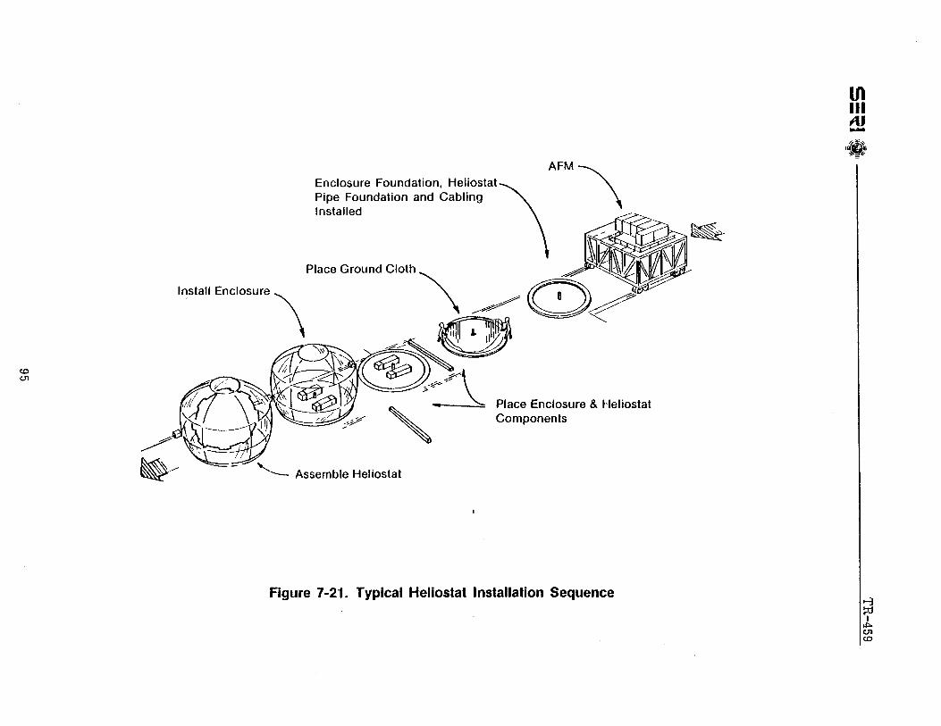
TR-459S=~I.'-----------------------Test Hardware to Pilot Plant. 'The National Science Foundation heliostat, the SubsystemResearch Experiment (SRE) hardware, and other future preproduction articles (Le., hard­ware constructed in small quantities in order to verify design/production feasibility) havebeen or will be produced in a typical way for test hardware using soft tools (nonperma­nent) and experiencing all the usual delays and first-time production problems. The na­ture of test hardware construction, if not trial and error, is at least one of a close, in­formal, and exacting association between engineers and manufacturing personnel.

Further, materials may not be delivered on time, they may be overprocured, or they maycome in totally "out of spec," and setup times and vendor tools must be allocated overonly a few units. Often, items must be reworked, causing additional setup or changes intooling. Finally, a great deal of time may be spent in working out specific methods foractually accomplishing particular manufacturing operations. As a result, labor and over­head are typically 5-15 times the cost of material, and materials are 4 or 5 times whatthey might cost for a pilot procurement.

The first major breakthrough in cost reduction will occur in the Barstow pilot plant helio­stat production. A production design is available and the quantities allow hard tooling,procurement discounts, scale economies, and standardized processes and balanced pro­duction flows typical of a working operation. It is difficult to project a true first-unitcost for such a scenario for comparison with test-unit cost because material costs arebased on vendor quotes for entire quantities, while labor hours are based on industrial en­gineering standards for a working production line. However, a synthetic first-unit cost,developed by extending unit pilot-plant costs on typical cost reduction curves, would beonly a quarter to a third the actual test article unit cost. Overall, labor and overheadcosts for pilot production will nearly equal materials costs and the average unit hours oflabor will be about 10% of the unit hours for the test articles.

Further cost reductions may occur in follow-on pilot production as a result of design-to­cost analysis. However, since ever-changing designs tend to inhibit cost reduction, muchof the potential will be latent, with changes apparent only where costs are immediatelydesigned out (e.g., elimination of inversion or of the site assembly facilities). Otherwise,the basic production facilities will change very little and each design variation will re­quire essentially a restart of production for the affected assemblies.

Pilot Produetion to Demonstration and Early Commercialization. As a result of prepro­duction and pilot production programs, a relatively firm design that will be suitable forcommercial production is expected to evolve. The prototype heliostat is representativeof such a design, although several changes have already been examined since completionof the study. This design allows considerable flexibility as to where and how the majorassemblies are fabrica ted and assembled.

The potential for strong but intermittent and uncertain growth in demand for any manu­facturer's product may give rise to a conservative attitude toward expansion. A rationalexpansion scenario suggests that modifying and expanding existing pilot facilities, in con­junction with added shifts and overboarding, and taking advantage of available capacityin other facilities, are necessary. Continued extensive procurement from other indus­tries will limit expansion pressures on resources, allowing much of the expansion to be in­dustrially financed. As a result, many of the purchased parts will have reached an estab­lished production status at this point.

96

TR-459S-~I ~_.. =~'-II II --------------------- _- '~-~

Cost-effective changes in the plant will reflect labor learning and managementlearning-about organizational requirements, production line flows, and so forth. As vol­ume expands, the manufacturer will be in a better bargaining position with suppliers,scale benefits will become apparent, and it may become necessary or cost-effective toadd or upgrade some equipment. Also, cost-effective design improvements that developor were planned as part of the prototype scenario but deferred until available, proven, orvolume justified may be incorporated on a part-by-part basis. In sum, although this is acautious, "make-do" period of expansion, a considerable cost reduction potential exists.

Early Commercialization to Nth Unit of Production. The primary issue during this periodis when and how the change-over to a large-scale, independent production facility shouldoccur. At least two possibilities exist. The first is to continually expand an existing fa­cility with added and upgraded equipment until a steady 25,000/yr production rate isachieved. This could cause some market share to be lost if cost reduction opportunitiesare delayed or capacity 5 reached before the new facility is completed.

The other possibility is to make the move when less than half of the 25,000/yr rate isreached. This could occur as early as the demonstration/early commercial period. As al­ready indicated, the facility may be operated on a one-shift basis at reduced capacitywith deferred purchase of some equipment. The most likely candidates would be certainau tomatic transfer equipment, or similar equipment (such as a bonding table).

AIthough the per-heliostat cost of the facility may double in the short run, the incrementmay be small compared with the savings potential of the new facility. It is likely thatthe increase would be more' than compensated by a reduction in average labor rate, re­duced hand labor headcount (Le., "hands-on" workers producing hardware either directlyor through operation of equipment), reduced overhead, and increased productivity causedby increased output per shift. As volume increases, the deferred equipment may beadded along with the second shift, contributing further to productivity and scale bene­fits. In addition, further procurement advantages will become apparent as suppliers rec­ognize both increasing volume and the growing stature of the program.

7.4.2 The Point of Steady-State Production

The point of steady-state production may be defined as that point in cumulative produc­tion volume where the only design changes permitted are those that may modify a partfor more effective production or performance, are for the primary purpose of cost reduc­tion, and will maintain a stable interface with other part concepts and designs. Simi­larly, the production process is a working, "debugged" operation representative of theeventual rate production plan. Generally, changes will be logical extentions of or im­provements upon existing processes, made only if the change permits a favorable rate ofreturn and involves an acceptable risk.

This definition does not exclude changes, but it is clear that research experiments, pre­production, and even pilot heliostat production facilities do not qualify because of theiruncertainties. It is equally clear that the prototype heliostat baseline production sce­nario would qualify because it is a steady-state scenario by definition. As conceived, thisscenario provides for the production and installation of 25,000 heliostats/yr, but by oper­ating on a one-shift basis, somewhat reducing line speed, and cutting the number of fieldcrews in half, identical facilities and equipment may be operated with a minimal, accept­able economic penalty at a rate of 10,000 heliostats/yr, or less. Thus, the prototype

97

TR-459S=~I_'-------------------------------baseline scenario, with minor modification, also may be used to describe a steady-stateproduction situation that could occur at a fairly early stage of cumulative production.

Accepting the modified scenario, the issue becomes a matter of determining how earlyan aggressive and dominant producer would plan initial operations in a new facilitycapable of producing approximately 10,000 heliostats/yr. In other words, at what pointmay the new production plant's initial operating capability (IOC) be aligned with the pro­ducer's cumulative sales volume expectations? Prior to this point in a producer's cumu­lative volume, it may be assumed that the production scenario is in an unstable statewhere designs and production plans are still subject to important changes. It follows thatthe determination of this point should provide the earliest stage in cumulative productionvolume, where it would be feasible to initiate operations under the defined steady-stateproduction scenario.

Relative to a market projection, this point of interest may be further defined as the ear­liest point in cumulative demand for a dominant producer's product, after which furtherdemand is able to absorb all the producer's future output at or greater than the steady­state production rate. A review of demand growth projections reveals the following pro­duction requirements:

• By the end of 1982, all suppliers will have produced 10,000 heliostats.

• During 1983 and 1984, an additional 10,000 heliostats will be supplied each year.

• In 1985, all suppliers must produce an additional 20-25,000 units in order to meetdemand projections.

• During 1986, 1987, and 1988, demand will approach 100,000, 150,000, and 300,000heliostats, respectively.

• Demand will continue to expand from 1988 through the turn of the century.

Accepting this market projection, an aggressive supplier desiring 40-50% of the marketcould plan its new facility IOC in 1985, in time to produce its 15,001st heliostat inaccordance with the modified baseline scenario. This corresponds to the electronicstechnology readiness date, and all other part configuration and production processes de­scribed as part of the prototype heliostat baseline production scenario. Assuming a 12­month startup, during which 5,000 heliostats are produced, the actual steady-state statuswill be achieved when the supplier has produced a cumulative total of 20,000 heliostats­15,000 of other designs in other facilities and 5,000 of the prototype heliostat design.

Whether or not this occurs in the manner described depends on how the individual firmactually views the strength of the market and associated risks. Of course, the strengthof the market depends on the quoted price of heliostats relative to alternative energycosts, and the extent of incentives for both suppliers and users. These variables are stillunknown. However, if successful cost reduction results in preproduction, pilot, and dem­onstration programs, by 1983 a manufacturer should be able to demonstrate to its ownsatisfaction that a move into baseline facilities will permit heliostat price quotes thatare quite competitive with alternate energy costs. As a result, an effective, steady­state production status for an aggressive, dominant supplier at the 20,000th unit is not anunreasonable projection under the circumstances.

98

TR-459S=~I i'.1 ----------------------------7.4.2.1 First-1Jnit ()osts

First-unit cost may be defined in a number of ways, depending on the perspective of theanalyst. In a development firm, it may be the cost of the first test article with or with­out a nonrecurr-ing engineering allocation, or a synthetic value extended from industrialengineering standards that have been determined at, say, the 100th unit of production.

A materials buyer for a new product may see the first-unit cost of a procured item as theaverage cost of the first lot in the door. The seller of the same item may see the pricecharged as that which the market will bear in order to recover a margin plus the averagecost to produce the item during the current year. The true first-unit cost for the itemmay be some unknown amount that occurred many years earlier. In a steady-state casesuch as this, the analyst is likely to consider the first unit cost as the sum of the cost perunit at the steady-state production rate plus an allocation of the incremental startupcosts that may be associated with introduction of a new model, introduction of new pro­duction equipment, or the initiation of a new production facility.

A marketer may be interested in developing a synthetic first-unit cost for use as a refer­ence in formulating downline pricing strategy. For this purpose, a product's current costexperience must be aligned with a unit of cumulative sales volume, as suggested in theprevious subsection, and the cost extended back on a historically representative cost re­duction slope to arrive at the synthetic first-unit cost. The resulting cost is syntheticbecause it represents a situation that usually is only hypothetically implied by currentproduction characteristics and the slope of the applied cost reduction curve. The rela­tionships between these definitions for the modified scenario will_become more apparentwhen the steady-state cost is quantified.

7.4.2.2 Development of Steady-State Unit Costs

The steady-state unit cost for the modified prototype heliostat scenario is developedusing two different methods. Both methods adjust the detail costing results presented inthe prototype heliostat study final repcr t for the 25,000-unit production rate. The firstmethod uses an aggregate resource impact approach, while the second employs cost re­duction curves applied to each detail line item. Both approaches arrive essentially at thesame total price at unit 20,000. Labor and overhead, however, are somewhat higher incost for the resource impact approach.

The results of the first method are shown in the steady-state cost column of Table 7-7.They address the four basic cost categories: factory labor, raw materials, purchasedparts, and field labor. The concept is to develop a logical adjustment reflecting thechanges in the scenario that permit reduced annual output. Since facilities and equip­ment remain the same, factory and field labor per unit stay essentially the same sincetotal labor would be cut in half in going from two shifts to one. However, to produce10,000 units/yr, line speed must be reduced 20%, which is assumed to increase hand labor25%. As a result of reduced use of the plant, the scale effect must be considered so thatoverhead is assumed to be 50% higher. Capital cost per unit will be somewhat more thandouble, while fringe benefits and a large share of other overhead items will vary more di­rectly with labor hours per unit. Direct support-including items such as sustainingtooling, industrial engineering, quality assurance, and manufacturing engineering-arealso assumed to increase 50% for reasons of scale.

99

S-~I. TR-459- :11:- ~~:."

Table 7-7. STEADY-sTATE COSTS

Costs (1978$)

Steady-State Synthetic EffectiveElement CRC Costs at 20,000 1st Unit 1st at 500

Factory Labor 89% $ 468 $2,973 $ 870

Ra w Material 98% 1,674 2,301 1,864

PurchasedParts 92% 1,250 4,667 1,948

Field Labor 98% 832 1,152 933

Total 94% $4,224 $11,103 $5,615

100

TR-459S=~I 'II!I -------------------------------

These adjustm ents have been applied to the labor and overhead costs at the prototypeheliostat's resource loaded peg point-the 125,000th unit. Costs were adjusted down alearning curve from this point to the 350,000th unit, and are thus slightly lower thancosts used for the adjustments described previously. Use of the costs at the peg pointprovides a more direct connection to the actual manloads developed for the prototypeheliostat report.

Materials costs were adjusted to include discounts. These costs were quoted by suppliersat rates of 25,000 units/yr over several years and reflect suppliers' discounts for fairlylarge quantities. At 4096 of these quantities, the discounts will be less. The changes indiscount are assumed as follows:

% Discount10,000 25,000

PriceImpact

Raw MaterialsInstallati on

15%26%

25%40%

1.131.23

The discount factors are based on cost analysis judgment, and the price impact shows theincrease applied to materials prices. For this analysis, all reflector unit and foundationrnaterials costs were treated as raw rna terials, although the prototype heliostat final re­port classified some of these elements (such as the sheet steel beams) as purchased parts.

The cost-reduction curve method extends the costs shown in the prototype heliostat re­port from the 350,000th unit (i.e., the midpoint unit in the 25,OOOth unit/yr scenario)back to the 20,OOOth unit. The same curves have been used that were employed to ex­tend the midpoint cost of the 25,OOO/yr baseline out to the midpoint cost projected forthe 250,000 unit/yr scenario. If labor increases approximately 10% a cost breakout isprovided that ties in with results determined using the resource impact approach.

Table 7-7 also shows the results of adjusting the steady-sta te cost column, using the costreduction curves shown, to reflect a synthetic first-unit cost and the effective cost atplant startup. The latter is calculated as the synthetic cost of the five hundredth unit,and is based on the determination that 500 units of equivalent experience are applicableto a calculation of plant startup costs.

Figure 7-22 shows these costs plotted in a log-log relationship. Translating a steady­state cost to an actual point on a cost-reduction curve can cause controversy. It is clearthat the cost should not be plotted as a first-unit cost, if only because the second unitwould be expected to be significantly less costly, while the average change in cost be­tween units in steady-state production will be very small. Similarly, it is probably notpreferable to plot the cost at even several thousand units further out in cumulative vol­ume. A point is finally reached, however, where such empirical arguments fade, so thatthe alignm ent of the steady-state cost and a point on a cost-reduction curve finally mustbe based on a feel for circumstances, some logic, and no small amount of judgment.

The steady-state cost is plotted at the 20,000th unit reflecting the attitude that thesteady-state cost actually represents costs associated with one heliostat's worth of re­sources and production time where the employment of resources is exactly as described,and the 20,000th unit is the earliest probable point where this situation exists exactly asdefined. Prior to this point, the producer will not have deployed and utilized this set ofresources as defined because of market conditions, technological conditions, and startupproblems. After the steady-sta te is reached, as defined, the resources and the manner of

101

TR-459S=~I '[W;, ------------------------------~-~ ~,

their employment will immediately start to change in response to market growth,innovation in product, process, equipment and manufacturing flows, influence onsuppliers, and similar cost reduction issues. Obviously, there is a margin of expectationin this analysis, so that the projection must be carefully considered.

The synthetic first-unit cost, as defined earlier, is also plotted along with the effectivefirst cost after plant startup using the data shown in Table 7-7. The plant startup cost isplotted at unit 15,000 and shows a rapid drop to the steady-state cost as prior heliostatexperience is used and production schedules and plans are brought to rate productiondefinition. These points are presented more to illustrate the concepts than as basic pa­rameters since they will vary around the steady-state projection, depending on the way afirm conducts its business and responds to market conditions.

The cost reported in the prototype heliostat study for the first 2,500 units is also plottedfor purposes of comparison. This cost reflects the prototype heliostat design but not thesteady-state production scenario. These heliostats are assumed produced in a pilot­plant-like production facility geared to a lower rate of production. The projected cost isapproximately 75% greater than the unit cost curve at 2,500 units, which is about what isexpected for this scenario since labor and overhead rates nearly double, productionequipment is much less sophisticated, procurement is apparent for only 2,500 units ratherthan 10,000 units/yr, and many production uncertainties still exist.

These projections have been developed using relatively general cost analysis methodsthat could be accomplished within the scope of the study. A more complete analysiswould obtain vendor quotes for each item of material at the production rates involved.Also, the impact on overhead and direct support labor would be examined in greaterdepth, and hand labor would be reviewed in detail in order to carefully screen the impactof line speed and double- to single-shift adjustments. Although a fair amount of revisionof the detail costs might be necessary if a more comprehensive analysis were needed, ag­gregate costs are probably within a reasonable range of accuracy. Even so, the main in­tention of this analysis has been to provide sufficient credible data so that the expecta­tions presented in this report may be adjusted to fit any variation in production circum­stances that might be considered. Above all, it should be recognized that the market andproduction scenarios, logic, and costs that have been presented here represent only oneof many ever-changing alternatives to the design, production, and marketing ofheliostats.

103

104

TR-459S=~I ![.~i -----------------------------­_~ ~~

SEC110N 8.0

DEVELOPMENT OF LEARNING AND COMPOSITE CURVES FORCOSTS ASSOCIATED WITH HELIOSTAT PRODUC110N*

The development of learning and composite curves, outlined in Sec. 3.0, can help predictoverall cost reduction in manufacturing the MDAC and GE prototype heliostat designs.The objective here is to project future costs for these designs using surrogate cost his­tory and the learning curve conceptual and analytical framework. First, selection of sur­roga tes will be discussed, followed by estimations of the learning and cost curves for sur­rogate products, and applications to heliostat assembly.

8.1 SELECTION OF SURROGATES

Each of the two heliosta t designs has been broken down into its components for purposesof cost analysis by both McDonnell Douglas Company and General Electric. The compo­nents are designated by WBS name and number as shown in Table 8-1.

Not all of the components and subassemblies are applicable to both contractors' designs.Surrogates for cost analysis have been chosen for selected components on the basis of thefollowing criteria:

• The relative importance of the component to the contractor's design;- .

• The relative contribution of the component to the total cost of the design; and

• The likelihood of availability of a meaningful surrogate having a body of histor­ical data.

The initial choice of components and surrogates to be analyzed and the design to whichthey are applicable is given in Table 8-2. As the study proceeded through the data col­lection phase, it became evident that other surrogate selections should be considered inaddition to or instead of those originally specified. An expanded listing of surrogatesused for this study is shown in Table 8-3.

The surrogates that were finally used for this study were chosen because manufacturingoperations between the surrogate and the heliostat components were close and reliablecost data were available. In several instances, the first surrogate chosen had to bechanged to another because of a lack of historical cost data. In other instances, as thestudy progressed, more appropriate surrogate parts with cost data became available. Thechanges made to the list of surrogates can be seen by comparing the surrogate selectionsin Tables 8-2 and 8-3.

*This section summarizes material presented in the report, "Development of SurrogateExperience Curves for Costs Associated with the Production of Heliostats," prepared byArthur D. Little, Inc., for SERI.

105

TR-459S=~II*'-----------------

Table 8-1. HELIOSTAT DESIGN COMPONENTS

WBS Number Part or Subassembly Name

4410441144124413

4420442144224423442444254426

4430443144324433

444044414442

4450445144524453

4460446144624463446444654466

Reflective UnitReflective SurfaceMirror Back StructureAssembly and Bonding

Drive UnitAzimuthElevationMotorsPosition IndicatorsPower DistributionAssembly of Drive and Pedestal

Control and InstrumentationSensorField Control ElectronicsControl Signal Equipment

Foundation and Site PreparationFoundationSite Preparation _

Heliostat Support and ProtectionHeliostat Support StructureHeliostat Protective EnclosureLightning Protection

Field Assembly and CheckoutHeliostatSensor Calibration EquipmentElectrical Power DistributionAlignment of HeliostatsField SupportPackaging and Transportation

106

TR-459S=~I.I----------------------

Table 8-2. CHOICE OF SURROGATES FOR HELIOSTAT COMPONENTS

DesignHeliostat Component Surrogates Applicability

l. Reflectors Laminated Mirrors McDonnell Douglas andPlywood Production General Electric

2. Elevation Actuator Machine Ball Screws McDonnell Douglas andGeneral Electric

3. Drive Controls Solid State Power McDonnell Douglas andControls and Condition- General Electric

ing

4. Pedestal Corrugated Tube McDonnell Douglas andWelded TUbing General Electric

5. Reflector Supports Conduit Raceway McDonnell DouglasDoor Mullions

6. Azimuth Gear Box Automative Gear Boxes McDonnell DouglasVariable Pitch Prop.Boxes

7. Azimuth Drive Hub Surveyors Wheels General ElectricBus/Truck Steering

WheelsComplex PrecisionPlastic Mold

8. Reflector Yoke Automobile Exhaust Tube McDonnell Douglasand General Electric

9. Reflector Enclosure Swimrning Pool Liners General ElectricWeather BalloonsBlow Molded Bottles

107

TR-459S=~I.I------------------------

Table 8-3. SURROGATES USED IN THE STUDY

DesignStatusaComponent Part Surrogate Applicability

1. Reflectors A. Plywood McDonnell +1. Total Douglas and2. Southern (New General

Industry) Electric3. Western (Old

Industry)4. Plywood and

Veneer5. Plywood

ManufacturerB. Aircraft Windshield +C. Laminated Mirrors +

2. ElevationActuator A. Aircraft Landing Gear McDonnell +

Douglas andGeneralElectric

B. Machine Ball Screws

3. Drive Controls (Single Chip Microprocessor)A. Personal Electronic McDonnell +

Calculators Douglas andB. Solid State Caleula- General

tors Electric

4. Pedestal A. Steel Pipes and Tubes McDonnell +B. Corrugated Tube Douglas andC. Welded Tubing General

Electric

5. ReflectorSupports A. Steel Wall Studs McDonnell +

B. Metal Door Sash and Douglas +Trim

C. Metal Household +Furniture

D. Conduit RacewayE. Door Mullions

6. Azimuth GearBox A. Drive Wheel Trans- McDonnell +

mission DouglasB. Automotive Gear BoxesC. Variable Pitch Prop.

a+Data have been obtained; -Data cannot be obtained.

108

TR-459S=~II,.1-------....,-----------------------

Table 8-3. SURROGATES USED (concluded)

DesignComponent Part Surrogate Applicability Statusa

7. Azimuth DriveHub A. Steering Wheel Bus, General Electric

TruckB. Harmonic Drive WheelC. Surveyors WheelsD. Complex Precision

Plastic Mold

8. Reflector Yoke A. Automobile Exhaust McDonnellTubing Douglas

B. Metal Household andFurniture General

C. Steel Pipes and Tubes Electric +D. Fabricated Pipes and +

Fittings

9. ReflectorEnclosure A. Swimming Pool Enclo- General

sure ElectricB. Aircraft Canopy +c. Blow Molded BottlesD. Weather BalloonsE. Helicopter Blade +

LinersF. Inflatable Shelters +

10. Assembly A. Truck/Bus Bodies McDonnell +B. Wing Structure Douglas +

and GeneralElectric

11. Overall Product A. Motor Vehicles McDonnell +B. Radio Telescope Douglas

and GeneralElectric

a+Da ta have been obtained; -Data cannot be obtained.

109

TR-459S=~II.!-------------------

All automotive-related surrogates (e.g., exhaust tubes, differentials, steering wheels) hadto be discarded because of the automotive industry did not release enough cost informa­tion. Despite several efforts, including those of a leading automotive industry consult­ant, no more definitive data than selling prices of automotive parts could be obtained.

During the course of the study, an exceptionally appropriate surrogate for the entireheliostat assembly was discovered in work sponsored by the U. S. Air Force at HanscomField, Mass, in 1962 [40]. The project involved the construction of a radio telescope de­sign to function in the same manner as the heliostats and tower. A multiplicity of indi­vidually oriented flat screen antennae were used to reflect radio waves emanating from adistant source. to a central receiver mounted in the tower. The plan was to use severalthousand antennae in an engineering installation. Unfortunately, only about 500 werebuilt and no mass production techniques were used. However, there were several designcycles for cost improvement that were completed within the course of the program.

The specific surrogates that were investigated for this study (see Table 8-3) have varyingdegrees of validity for heliostat component counterparts and varying levels of cost dataquality. Surrogate validity and data fidelity cannot be measured quantitatively. Someinferences regarding the quality of the data, however can be drawn statistically. Aqualitative judgment can be made regarding the validity of the surrogate as an analogue.

The use of aircraft windshields and laminated mirrors for surrogates of heliostat reflec­tors represents a very close match of materials and manufacturing processes. The use ofplywood as an analogue of the reflector is less directly related in terms of material butsimilar in terms of manufacturing processes. Plywood manufacturing requires thebonding of friable, delicate laminates into a continuous, multilayered structure. Al­though plywood manufacturing is an old, well established industry, there are segments(such as the southern plywood industry) that are relatively new. Learning effects wouldprobably be more prevalent in such new industries.

The elevation actuator is an electromechanical positioning system. While the machineball-screw mechanism is a very close surrogate, no cost data were available for it. Theaircraft landing gear is a similar electrohydraulic mechanical system which requires finemechanical design, careful machining and assembly, and a high level of reliability. Al­though the landing gear surrogate is probably more complex than the elevation actuator,the configuration, materials, and manufacturing operations are probably quite similar tothe elevation actuator component.

The drive controls and their costs are dominated by the microprocessor or control com­ponent. The other components of the control system are necessary to the design but aregenerally purchased elsewhere and assembled. The electronic calculator is a reasonablesurrogate in that its cost is also dominated by a single chip microprocessor, despite aneed for other electronic and structural components.

The pedestal is a difficult component for which to find surrogates with meaningful his­torical cost data. Steel pipes and tubes (welded or seamless) are manufactured using anold technology. Early cost data are virtually lost, and recent data would exhibit little (ifany) learning effect. We have nevertheless included these because of the dearth of infor­mation related to any other potential surrogates. Furthermore, the fact that manufac­turing of tubular components is a well developed technology indicates that if manufac­turers skilled in the art are used, the learning effect in manufacturing these componentswould be minimal.

110

TR-4595=~1 'I.~i------------------------- .;Several surrogates are available for the reflector supports. The least realistic are thefabricated pipes and fittings. However, the rolled steel sheet shapes used in steel wallstuds and metal door sashes are completely analogous to the steel channel configurationof the reflector supports. These surrogate industries are well developed and mature.Learning effects, however, are probably not evident. Of course, there may also be littlelearning in fabricating as simple a structure as the reflector supports.

The surrogates for the azimuth gear box were chosen because they represent mediumprecision gear trains that were produced in medium volumes of tens of thousands peryear. The only choice including manufacturing cost data involved the transaxle transmis­sion of an off -the-road vehicle such as a tractor. The data is given for a completely newdesign, from its inception four years ago to the present. The results indicate that, whilelearning occurs, the design and fabrication of transmissions by people skilled in the artwill avoid most of the early costs associated with new designs.

Data for the azimuth drive hub was not available for any of the selected surrogates.Manufacturers of automotive steering wheels and harmonic drives would not release costdata. Other sources such as industry associations and plastic parts suppliers also provedto be of no help. For this study, it was conservatively assumed that the current manu­factured estimated cost by General Electric would not change much.

The surrogates for the reflector yoke resulted in much the same data as the pedestal sur­rogates. No data were directly available from manufacturers or manufacturers' associa­tions. The data available at this time are weak. However, because of the nature ofthese parts, significant learning should not be expected.

Several surrogates yielded good quality data for the reflector enclosure. The aircraftcanopy, helicopter blade liners, and inflatable shelter provided valid cost data. The heli­copter blade liners and inflatable shelter are closer in manufacturing process and rnate­rial to the processes used for the reflector enclosure.

Originally, no surrogate was selected to represent the assembly operation. Essentially,the heliostat is a mechanical configuration requiring assembly of structural compo­nents. The aircraft wing structure assembly operation is an excellent analogue for whichvalid cost data are available from the manufacturer. The learning effect is typical ofwhat may be anticipated for the assembly of the heliostat units.

For the overall product no reliable surrogate data were available. As previously dis­cussed, the radio telescope antenna assembly represents the penultimate surrogate for aheliostat, Unfortunately, none were ever mass-produced.

8.2 DERIVATION OF LEARNING AND EXPERIENCE CURVES FOR SURROGATES

8.2.1 Data Acquisition

As noted previously, surrogate products were identified and selected under the assump­tion that historical (relative) cost pa ttems exhibited by these products could apply tocorresponding heliostat components as well. Furthermore, in order to be applicable tothe heliostat assembly, the relative cost behavior for each surrogate must be independentof ancillary conditions such as:

III

TR-459S=~I.i- ---------

• years of production,

• annual production rates, and changes in ra tes,

• absolute unit costs of surrogates,

• economic factors,

• production volume, lot sizes, and sequence numbers used, and

• extraneous factors that might distort the constant rate of reduction in unit cost.

Thus, it is assumed that cost reduction (or increase) is constant over time, and can be es­timated from the observed slope parameter (b) for the surrogate products selected. Ifthe raw cost/quantity data have been influenced in any way to distort the "true" slope ina substantive manner, these effects must be estimated and data adjustments made, orassumed negligible. An excellent example of this type of problem is illustrated at theconclusion of this section.

After an acceptable list of surrogates was constructed, the next step was to acquiremeaningful production cost data. The original intent was to gather historical cost datafor each surrogate product, broken down according to labor, materials, and overhead.Furthermore, sources of cost reduction and extraneous factors were to be determined inthe manufacturing of surrogate products.

The data acquisition task proved to be a formidable one, so cost data presented in thissection are of limited quality. For the surrogate approach to be credible, it is imperativethat accurate and reliable cost data be used, and that the manufacturing history of eachcomponent be well understood. In view of unexpected and unavoidable difficulties en­countered in acquiring reliable cost data for many surrogate products, it is recommendedthat the derived learning percentages be accepted with caution, and that absolute valuesand ranges be considered illustrative rather than definitive.

The data acquired for this study were provided by Arthur D. Little, Inc., and are summa­rized in the tables presented in Appendix A. Data sources are identified except whenconfidentiality was requested. Some comments concerning the data contained in those20 tables are listed below.

• All dollar amounts given were normalized within each table, to account for infla­tion, and are internally consistent for each surrogate.

• Since cumulative production quantities are required, only sequential productionvolumes are included; for example, plot points for the data in the first table arecalculated from the true cumulative production figures since 1960.

• In cases where production quantities were not available, plot points were cal­culated from normalized material costs. This technique assumes that observeddifferences in deflated materials costs reflect production level changes only andthat materials unit costs remain constant.

• Prior cost/quantity history is ignored. Data are assumed to reflect "normal"learning even though mature industries such as motor vehicles might have be­haved quite differently at the outset.

• Tabulated data given in this report have been summarized; more detailed rawdata were extracted from most sources indicated.

• In all cases, total cost includes direct labor, materials, and overhead.

112

TR-459S=~I :111

-------------------

8.2.2 Surrogate Learning Curve Estimation

After all relevant data had been accumulated, unit costs and corresponding cumulativeproduction quantities were calculated according to the scheme presented in Appendix B.In most cases, the average cost of producing the nth unit was considered; however, a fewcumulative cost curves were also generated primarily for comparative purposes. Cost/quantity data pairs were subsequently coded for computer processing. A least-squareslinear fit (on log-log scale) was then performed using the BMDP Biomedical ComputerProgram subroutine BMDPIR, Multiple Linear Regression. The complete output of thisprogram is illustrated in Appendix B.

The output presents several summary statistics of interest, including the followingr

• The estimated least-squares line; i.e., the intercept parameters (log a) and theslope (b);

• The standard error of the regression coefficient estimate (b); under certainassumptions, this term can be used to ealoula te confidence interval estimates forthe slope;

• R (the sample correlation coefficient) and R2 (which measures the proportion ofvariation in log cost explained by the linear model);

• The standard error of estimate, which measures the dispersion of the observa­tions about the estimated regression line; and

• The probability that a test statistic calculated from the data (the F-ratio) wouldbe as large as observed if, in fact, the two variables were-not linearly related; asmall probability implies rejection of the hypothesis of no linear relationship.

A plot of observed log cost (0) and predicted log cost from the least-squares equation (P)is also given in log-log units. The plot of residuals (observed minus predicted log costs) isalso given for purposes of validating an important underlying assumption of regressiontheory. This assumption refers to the independence of observed C values; that is, in re­gression theory it is assumed that successive observations are independent of one an­other. This assumption is clearly violated in cumulative cost curves, and is difficult tojustify in unit cost data as well. Nevertheless, probability statements in the form of 95%confidence interval estimates are presented in Appendix A, Table A-21, which summa­rizes all regression runs performed. Therefore, if regression assumptions are accepted,the probability is 0.95 that the learning rate interval given includes the "true" (unknown)learning rate that we are attempting to estimate from these data.

The effect of variability in slope estimates, as well as overall precision in the estimationtechniques, is demonstrated in Fig. B-3 (see Appendix B) using the Aircraft Canopy sur­rogate data. Three lines are drawn to indicate upper (80%) and lower (58%) bounds, andthe regression estimate itself (68%), since these estimators are subsequently applied inthis study to actual heliostat components.

In the usual application of learning curve theory, this regression line would be used topredict the unit cost of producing additional canopies. Two different, and often misun­derstood, interval estimates are also illustrated in Fig. B-3 for this situation. The nar­rower band depicts a 95% confidence interval estimate about a conditional mean costvalue; the wider band represents the more commonly required prediction interval concernwith the estimation of only one individual unit cost. For example, it can be stated with95% confidence that, on the average, the cost of producing the 200th canopy would be

113

TR-459S=~II.'--------------------

between 4.7 and 13 hours; however, the data also indicate that the predicted cost of the200th canopy produced in this sequence can be expected to be between 2.9 and 22 hours,a much broader, less precise estimate. In addition to displaying this distinction betweenconfidence and prediction intervals, this figure is intended to illustrate the following:

• Variation in slope can have dramatic effects on unit cost estimates;

• An apparent "reasonable good" linear fit (R2 =0.88) does not necessarily yield es­timates or predictions of acceptable (i.e., useful) precision; and

• Regression theory, if appropriate at all, works best near the mean of the data;extrapolating beyond the observed data is risky and subject to large estimationerrors.

There are additional limitations to applying historical learning trends to different, butrelated, components. For example, the following concerns are worth noting:

• Learning curve slope estimates are highly dependent on the particular surrogateselected; different surrogates intended to characterize the same heliostat com­ponent can yield vastly different estimates of learning effects.

• Identical surrogates, such as plywood, lead to widely varying estimates dependingon the data source, age of industry, and other variables, such as geographical 10­cation.

• There is evidence that learning dampens out for mature industries and, therefore,may not represent expected patterns for similar components with different sys-tem configurations and/or requirements. -

• Estimated slopes appear to depend on units of measure, even in situations thatshould be invariant; e.g., see Appendix A data on number of workers (b = -0.59),hours worked (b = -0.33), and standardized labor cost (b = -0.65).

• Many of the surrogates used in this study indicated little or no measurablelearning. This condition manifested itself in two ways: 0) the data did notappear to be linearly related as measured by standard goodness-of-fit test sta­tistics, and/or (2) unit costs were constant, and apparently unrelated to quantityproduced over the range of production units considered.

• Estimates for heliostat components are highly subjective, even if the surrogatecost/quantity data were reliable in all respects.

• Historical "raw" cost data can be, and frequently are, contaminated with hiddeneffects that only extraordinary and detailed investigation will uncover. Ex­amples of this type of unusual cost/quantity behavior are given in Appendix A, intwo sets of cost data. In Tables A-16 and A-19, one column, denoted as "actual"unit cost, represents costs incurred to produce the corresponding lot sizes. Theother cost column, entitled "adjusted" unit cost, reflects the results of a compre­hensive study conducted by Arthur D. Little, Inc., which yielded substantive evi­dence that "actual" costs were inflated and unusually high for early productionunits because of circumstances unique to a particular production program. Suchuniqueness is not uncommon in the literature.

114

TR-459S=~II.I --------------------------:-------

8.3 APPIlCATION TO HEUOSTAT ASSEMBLY

8.3.1 Unit Cost Estimates for Relevant Components

The prototype heliostat investment cost estimates for various annual production levelsfor MDAC and GE design configurations are presented in Subsection 7.3. Tables 8-4 (GE)and 8-5 (MDAC), provide the average investment cost per heliostat estimates for thebaseline plant (25,000 units/yr), For the MDAC Prototype Heliostat Study (3) it wasassumed that plants will initiate operations after 100,000 heliostats have been producedfor pilot plants, demonstration plants, and the first commercial plants. However, the av­erage investment cost per heliostat has been projected as that required at the start ofthe second year of rate production in the factory, or at unit 125,000 [3, pp, 9-21].

The 25,000 units/yr scenario, representing the plans associated with a well conceived, ad­vanced design, has been developed as the baseline scenario. This rate represents a signif­icant high-volume production situation and reflects conditions required to establish asteady-state production process. Also, it may be easily translated into both higher orlower productive capacity. Thus, this scenario lends visibility to the development of vi­able business constraints and at the same time supports astra tegy for capturing animportant share of eventual markets. As indicated before, the 25,000 heliostats/yr pro­duction rate represents only one of many possible scenarios.

8.3.2 Development of Heliostat Component Cost Curves

The procedures for using learning and cost curves to predict cost -reduction in manufac­turing solar technologies outlined previously show that learning and cost curves were tohave been derived and aggregated over labor, materials, and overhead cost elements foreach heliostat part. Since the data collected are not amenable to treatment at this levelof detail, the conceptual framework will be illustrated with total cost data only.

Learning curve slope estimates observed for the surrogates were superimposed on thesingle point estimate assigned to the 25,000th unit. Again, the criterion for selecting arepresentative slope estimation from among two or more alternatives was essentiallysubjective. In each case, upper and lower bounds were also prescribed to emphasize theimportance of using interval estimation; these bounds, however, are not purported to beconfidence limits, and probability statements do not apply. The technique is illustratedfor the GE design and the MDAC design in Appendix C.

8.3.3 Aggregation of Costs

A composite cost curve was then constructed for each heliostat design configuration byaggregating costs at similar production quantity levels over the 11 individual componentparts. To illustrate the aggregation process, boundary value cost curves are generated bysumming high and low costs, respectively, in addition to the "expected" value determinedfrom the "most likely" learning slope. As before, these boundary values have no statis­tical (i.e., probabilistic) meaning, and are included for illustrative purposes only. Theaggregate cost curves are given in Fig. 8-1 and 8-2 for the GE and MDAC designs, re­spectively. As these curves indicate, the conceptual estimation technique examined inthis study would almost certainly yield a nonlinear cost/quantity relationship for theoverall assembly since slopes are not additive over components in a log-log scale.

115

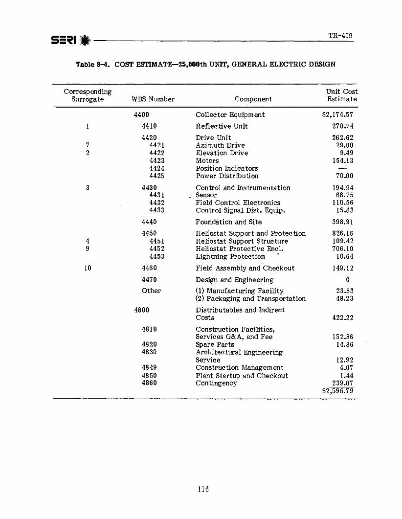
TR-459S=~I.J-------------------------

Table 8-4. COST ESTIMATE-25,OOOth UNIT, GENERAL ELECTRIC DESIGN

Corresponding Unit CostSurrogate WBS Number Component Estimate

4400 Collector Equipment $2,174.57

1 4410 Reflective Unit 270.74

4420 Drive Unit 262.627 4421 Azimuth Drive 29.002 4422 Elevation Drive 9.49

4423 Motors 154.134424 Position Indicators4425 Power Distribution 70.00

3 4430 Control and Instrumentation 194.944431 Sensor 68.754432 Field Control Electronics 110.564433 Control Signal Dist, Equip. 15.63

4440 Foundation and Site 398.91

4450 Heliostat Support and Protection 826.164 4451 Heliostat Support Structure 109.429 4452 Heliostat Protective Encl. 706.10

4453 Lightning Protection 10.64

10 4460 Field Assembly and Checkout 149.12

4470 Design and Engineering 0

Other (1) Manufacturing Facility 23.83(2) Packaging and Transportation 48.23

4800 Distributables and IndirectCosts 422.22

4810 Construction Facilities,Services G&A, and Fee 152.86

4820 Spare Parts 14.864830 Architectural Engineering

Service 12.924849 Construction Management 4.074850 Plant Startup and Checkout 1.444860 Contingency 239.07

$2,596.79

116

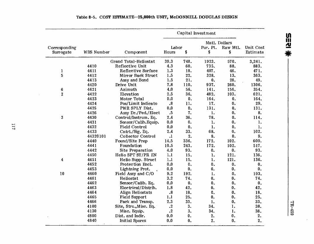
Table 8-5. COST ESTIMATE-25,OOOth UNIT, McDONNELL DOUGLAS DESIGN

Capital Investment IIIMati. Dollars III

--UCorresponding Labor Pur. Pt. Raw MH. Unit Cost -

Surrogate WBS Number Component Hours $ $ $ Estimate ,fill'.: ~~'

Grand Total-Heliostat 39.3 748. 1923. 570. 3,241.4410 Reflective Unit 4.3 60. 735. 88. 883.

I 4411 Reflective Surface 1.3 18. 407. 46. 471.5 4412 Mirror Back Struct 1.5 22. 328. 13. 363.

4413 Assy and Bond 1.5 21. o. 28. 49.4420 Drive Unit 7.8 110. 937. 260. 1306.

6 4421 Azimuth 4.0 56. 141. 156. 354.2 4422 Elevation 2.5 36. 482. 103. 621.

4423 Motor Total 0.0 o. 164. o. 164.4424 Pos/Limit Indicate •8 II. 17. o. 29•4425 PWR SPLY Dist. 0.0 o. 131. o. 131.4426 Assy Dr./Ped./Elect •5 7. I. o. 8•

3 4430 Control/Instrum. Eq. 2.4 36. 78. o. 114.

~4431 Sensor/Calib.Bquip, 0.0 o. I. o. 1.

..... 4432 Field Control 0.0 o. I. o. 1.-a4433 Cntrl./Sig. Eq. 2.4 33. 68. o. 102.44320101 Collector Control .1 2. 8. o. 9.4440 Found/Site Prep 14.5 336. 172. 102. 609.4441 Foundation 10.5 243. 172. 102. 517.4442 Site Preparation 4.0 93. o. o. 93.4450 Helio SPT ST/PR EN 1.1 IS. 1. 121. 136.

4 4451 Helio Supp. Struct 1.1 15. 1. 121. 136.4452 Protection Encl. 0.0 o. o. o. o.4453 Lightning Prot. 0.0 o. o. o. o.

10 4460 Field Assy and C/O 9.2 192. 1. o. 193.4461 Heliostat 3.2 74. o. o. 74.4462 Sensor/Calib. Eq, 0.0 o. o. o. o.4463 Elec trical/Distrib. 1.8 42. o. o. 42.4464 Align Heliostats .8 18. o. o. 18.4465 Field Support 1.1 25. o. o. 25.4466 Pack and Transp. 2.3 33. 1. o. 33. ~

4100 Site, Stru.,Misc. Eq•. .2 3. 34. 1. 38. ~I

4130 Misc. Equip. .2 3. 34. 1. 38. ~en

4800 Dist. and Indir, 0.0 o. 2. o. 2.(0

4840 Initial Spares 0.0 o. 2. o. 2.

TR-459S=~I,_,-------------------

The MDAC heliostat assembly composite unit cost curve starts out at approximately94%, changes to 96%, and finally reaches 97%.

Table 8-6. ESTIMATED COSTS AND SLOPES FOR THE MDAC HELIOSTAT DESIGN

Quantity Heliostat Investment Cost Composite CurveProduced $ Per Heliostat Slope (%)

1,000 4,12893.8

2,000 3,87394.1

4,000 3,64595.1

8,000 3,46895.7

16,000 3,31996.1

32,000 3,18996.7

64,000 3,085

100,000 3,017 97.3

While, for the same production scenario, the GE heliostat assembly composite unit costcurve starts out at approximately 89% changes to 92% and 94%, and finally reaches 99%.

Table 8-7. ESTIMATED COSTS AND SLOPES FOR THE GE HELIOSTAT DESIGN

QuantityProduced

1,000

2,000

4,000

8,000

16,000

32,000

64,000

100,000

Heliostat Investment Cost Composite Curve$ Per Heliostat Slope (%)

4,10688.7

3,64089.5

3.25890.9

2,96292.0

2,72393.0

2,53394.0

2,382

2,287 99.0

120

TR-459S=~I !I.I -------.,.-------------------------

SECTION 9.0

REFERENCES

1. Drumheller, K. Heliostat Manufacturing Analysis. EY-76-C-O 6-18 30. Prepared forthe United States Department of Energy. Richland, WA: Pacific Northwest Laberratory; Oct. 1978.

2. Electric Power Research Institute Heliostat Cost Study. Cambridge, MA: ArthurD. Little, Inc., et al.

3. McDonnell Douglas Astronautics Company, West. Solar Central Receiver Proto­type Heliostat CDRL Item B.d Final Technical Report. Vol. I and II. MDCG7399.Huntington Beach, CA: McDonnell Douglas Astronautics Company; Aug. 1978.

4. General Electric. Solar Central Receiver Prototype Heliostat Phase I. Final Tech­nical Report. SAN-1468-I. Schenectady, N.Y.: General Electric; Oct. 1978.

5. Petruschel, R. L. The Derivation and Use of Estimating Relationship, Memorandum#RM-3215-PPR. Santa Monica, CA: The Rand Corporation; Feb. 1962.

6. Fisher, G. H. Derivation of Estimating Relationships: An illustrative Example.Prepared for the United States Air Force Project Rand, Memorandum RM-3366­PRo Santa Monica, CA: The Rand Corporation; Nov. 1962.

7. Walters, A. A. "Production and Cost Functions: An Econometric Survey." Econo­metrica. Vol. 31: Jan. 1963; pp. 1-66.

8. Conway, R. W.; Schultz, Andrew Jr. "The Manufacturing Progress Function," TheJournal of Industrial Engineering. Vol. 10: Jane-Feb, 1959; pp, 39-54.

9. Krawiec, F.; Flaim, T. Solar Cost Reduction Through Technical Improvements:The Concepts of Learning and Experience. SERI/RR-52-173D. Prepared for theU.S. Department of Energy. Golden, CO: Solar Energy Research Institute; Feb.1979.

10. Costello, Dennis; et al. Photovoltaic Venture Analysis; Progress Report. SERI­23. Golden, CO: Solar Energy Research Institute; Apr. 1978.

11. Young, Samuel L. "Misapplications of the Learning Curve Concept". The Journalof Industrial Engineering. Vol. XVII (No.8): pp, 410-415.

121

TR-459S=~I_I------------------------

12. Colasuonno, Vincent. An Analysis of Progreg; Curve Conceptual Advances andProgreg; Curve Uses Since 1956. M.S. thesis. Air University; 1970.

13. Orsini, Joseph A. An Analysis of Theoretical and Empirical Advances in LearningCurve Concepts Since 1966. M.S. thesis. Air University; 1970.

14. Hirsch, Werner F. "Manufacturing Progress Functions." Review of Economics andStatistics. Vol. 34: May 1952; pp. 143-155.

15. Andress, Frank J. "The Learning Curve As a Production Tool." Harvard BusinessReview. Vol. 32: Jan.-Feb. 1954; pp, 87-97.

16. Baloff, Nicholas. "Extensions of the Learning Curve: Some Empirical Results."Operational Research Quarterly. Vol. 22: Dec. 1971; pp. 329-340.

17. Wright, T. P. "Factors Affecting the Cost of Airplanes." Journal of AeronauticalScience. Vol. 1: Feb. 1936; pp. 122-128.

18. Pegels, C. Carls. "Start Up or Learning Curves-Some New Approaches." DecisionSciences. Vol. 7: 1976; pp. 39-54.

19. Asher, Harold. Cost Quantity Relationships in the Airframe Industry. R-291.Santa Monica, CA: The Rand Corporation; July 1956.

20. Reguero, Miguel A. An Economic Study of the Military Airframe Industry. AnnArbor, MI: University Microfilms International; 1957.

21. Billion, S. A. "Industrial Learning Curves and Forecasting." Management Inter­national Review. July 1965; pp. 65-96.

22. Harting, W. G. Cost Estimate Errors Resulting from the Use of Learning CurveMethods. L. G. Hanseem Field, MA: Escer, Electronic Systems Division; Aug.1969.

23. Ferguson, C. E. The Neoclag;ical Theory of Production and Distribution. London:Carnbrldge University Press; 1971.

24. Brewer, Glenn M. The Learning Curve in the Airframe Industry. M.S. thesis. AirUniversity; 1965.

122

TR-459S=~I ,i.i ---------------------------- .

25. Morse, Wayne J. "Learning Curve Cost Projections with Constant Unit Costs."Managerial Planning. Marc-Apr, 1974; pp. 15-21.

26. Hirschmann, Winfred B. "Profit from the Learning Curve." Harvard BusinessReview. Vol. 42: Jan.-Feb. 1964; pp. 125-139.

27. Boston Consulting Group. Prospectives on Experience. Boston, MA: 1972.

28. Bodde, David L. "Riding the Experience Curve." Technology Review. Mar.-Apr.1976; pp, 53-59.

29. Yelle, Louis E. "Estimating Learning Curves for Potential Products." IndustrialMarketing Management. Vol. 5: 1976; pp, 147-154.

30. Seherer, F. M. Industrial Market Structure and Economic Performance. Chicago,IL: Rand McNally Publishing Co.; 1970.

31. Salter, W.E.G. Productivity and Technical Change. 2nd ed, London: CambridgeUniversity Press; 1966.

32. Small Power Systems Study. Quarterly Report No.1. SERI-36. Golden, CO: SolarEnergy Research Institute; July 1978.

33. Recommendations for the Conceptual Designs of the Barstow, California, SolarCentral Receiver Pilot Plant. Executive Summary. SAND-77-8035. Sandia Labo­ratories; Oct. 1977.

34. Solar Central Receiver Prototype Heliostat. Phase 1, Final Technical Report.SAND-1468-I. Schenectady, N.Y.: General Electric; Oct. 1978.

35. Conceptual Design of Advanced Central Receiver Power System. Phase 1, Execu­tive Summary. Martin Marietta Corp.; Sept. 1978.

36. Prototype/Second-Generation Heliostat Evaluation and Recommendations. Execu­tive Summary. SAND-78-8265. Sandia Laboratories; Oct. 1978.

37. Vant-Mull, L. L. "Development of Solar Tower Program in the United States."Optical Engineering. Vol. 16 (No.6): Nov.-Dec. 1977.

123

TR-459S=~I '.1 ---------------------------__

38. Marshall, B. W. "Operation of the Solar Thermal Test Facility." Department ofEnergy Large Solar Central Power Systems Semiannual Review. SAND-78-85ll.Sandia Laboratories; Nov. 1978.

39. Wilson, W. G. "An Overview of the Heliostat Development Program." Proceedingsof the 1978 DOE Workshop on System Studies for Central Solar Thermal Electric;Mar. 27-30, 1978. University of Houston Solar Energy Laboratory; Oct. 1978.

40. Schell, Allen C. Preliminarv Design Study of a Flat Plate Reflector and SupportUnit. Hughes Aircraft Co.; May 1964.

41. Nourse, J.H. Prototype Heliostat Costing Scenario. Final Report. HuntingtonBeach, CA: McDonnell Douglas Astronautics Company; July 1979.

42. Development of Surrogate Experience Curves for Costs Associated with the Pro­duction of Heliostats. Final Report. Cambridge, MA: Arthur D. Little, Inc.; Sept.1979.

124

TR-459S=~I.i--------------------------

APPENDIX A

SUMMARY OF DATA ACQUIRED FOR SELECTED SURROGATE PRODUCTS

125

126

TR-459S=~I~.I ----------------------------

Table A-I. SURROGATE lA-PLYWOOD (TotaI)R

LaborProduction No. of Hours Cost(feet x 109) Workers Worked (x 103)

Year Annual Cumulative (per million feet of production)

1960 7.8 75.3 b4.9b1965 12.6 127.7 3.5b1970 14.1 195.4 2.8

1972 17.8 229.6 2.2 5.04 $12.641973 17.9 247.6 2.3 4.97 10.941974 15.3 262.9 2.4 5.12 12.581975 15.7 278.6 2.2 4.54 11.411976 17.8 296.4 2.2 4.78 10.961977 19.7 316.1 2.1 4.55 9.58

aSource: American Plywood Association.bEstimates derived from employment figures for softwood plus hardwood plywood.

Table A-2. SURROGATE lA-PLYWOOD (West)R

Production Direct Material Total(feet x 109) Labor Cost Cost

Year Annual Cumulative (per 103 feet)

1965 11.3 125.0 $15.95 $30.58 $58.511970 10.1 177.4 17.12 35.06 65.901975 9.3 231.3 15.27 33.27 60.801977 10.7 263.3 12.97 29.39 51. 74

a American Plywood Association.

127

TR-4595=~1'.'------------------

Table A-3. SURROGATE lA-PLYWOOD (South)a

Production Direct Material Total(feet x 109) Labor Cost Cost

Year Annual Cumulative (per 103 feet)

1965 1.14 1.62 $10.23 $25.12 $54.211970 3.32 11.96 6.69 27.17 55.001975 5.68 38.06 6.66 24.25 48.581977 7.45 52.32 6.02 20.95 40.30

aAmerican Plywood Association.

Table A-4. SURROGATE lA-PLYWOOD CORPORATIONa

Year Production Manhours

1966

1967

1968

1969

1970

1971

1972

1973

1974

1975

1976

1977

1978

1979

8,299

34,393

46,945

46,679

48,208

59,063

55,345

48,729

47,247

50,678

55,146

57,230

59,559

34,914

55,019

290,439

.262,377

239,186

248,176

291,685

301,930

271,029

276,036

293,496

309,799

317,840

324,830

168,044

aConfidential source (plywood Corporation).

128

TR-459S=~I ';.~l-----------------------~ '.

Table A-5. SURROGATE lA-PLYWOOD AND VENEERa

Direct Material TotalProduction Labor Cost Cost

Year (tons x 106) (x 106) (x 106) (x 106)

1967 7.7 $335.7 $931.4 $1,384.41968 8.6 322.1 946.4 1,377.91969 8.0 300.1 925.9 1,334.71970 8.3 332.7 990.1 1,446.41971 9.7 346.8 1,103.6 1,579.41972 10.4 357.8 1,218.7 1,702.91973 10.4 326.4 1,187.3 1,628.71974 9.0 NA NA NA1975 8.7 386.8 1,132.9 1,534.51976 9.9 295.4 1,230.4 1,638.0

a Predicasts.

Table A-6. SURROGATE I B-AIRCRAFT WINDSmELD8

No. of Units Geometric _ Unit CostProduced in Lot Meanb (Direct Labor Hours)

4 2.2 97

4 6.4 79

22 20.6 149

4 31.3 181

3 32.4 468

9 52.7 190

35 59.3 153

42 137.0 94

35 146.8 73

15 203.0 182

29 238.5 92

18 241.4 141

aConfidential source (aircraft manufacturer).bUnits were not produced sequentially within lots; plot points were

calculated according to geometric mean of actual production sequence.

129

TR-459S=~I il.' _

Table A-7. SURROGATE IC-LAMINATED MmRORSa

Direct Material TotalLabor Cost Cost Cost

Year (x 106) (x 106) (x 106)

1967 $27.12 $81.97 $125.11968 28.09 86.72 131.31969 30.54 97.54 146.91970 29.08 84.26 132.71971 30.70 97.55 148.11972 42.67 135.69 205.61973 44.59 138.69 211.71974 46.47 135.08 211.71975 49.94 141.82 241.61976 52.80 162.32 253.9

a Predicasts.

Table A-8. SURROGATE 2A-AIRCRAFT LANDING GEARa

No. of UnitsProduced in Lot

GeometricMeanb

Unit Cost(Direct Labor Hours)

4

4

22

4

3

9

35

42

35

15

29

18

3.9

5.4

18.8

29.5

31.2

45.7

60.5

114.6

121.5

161.9

196.0

197.4

238

218

124

140

100

111

97

135

107

155

157

79

aConfidential source (aircraft manufacturer).bUnits were not produced sequentially within lots; plot points were

calculated according to geometric mean of actual production sequence.

130

TR-459S=~I i'*'1 ------------------------- .~

Table A-9. SURROGATE 3A-PERSONAL ELECTRONIC CALCULATORSa

Direct Material TotalProduction Labor Cost Cost

Year (tons x 106) (x 106) (x 106) (x 106)

1974 12.0 $130 $415 $6031975 16.0 84 320 5131976 17.5 43 196 3161977 18.7 65 244 393

a Predicasts,

Table A-IO. SURROGATES 4A AND 8C--5TEEL PIPES AND TUBESa

Year Prod. Labor Materials Overland Total

1967 .206 1.000 .099 1.305

1968 .229 1.126 .113 1.468

1969 .267 1.236 .138 _ 1.641

1970 .238 1.014 .133 1.385

1971 .257 1.188 .152 1.597

1972 .331 1.469 .178 1.978

1973 .423 1.908 .217 2.548

1974 .613 3.416 .326 4.355

1975 .735 4.037 .421 5.193

1976 .714 3.687 .431 4.832

a Predicasts.

131

TR-459S=~II*i_---__-----------

Table A-H. SURROGATE 5A-sTEEL STUDSa

Year

19751976197719781979

Production Materials Other Cost/Ft(feet x 103) Cost/Ftb (incl. Profit Margin)b

150.1 $.116 $.063506.0 .126 .059

1196.0 .137 .0591176.0 . .149 .0581067.0 .169 .044

aConfidential source (building component manufacturer).bEstimate from price data and wholesale price index for galvanized carbon steelsheets.

Table A-12. SURROGATES 5B-METAL DOOR SASH AND TRIMa

Year Prod. Labor Materials Overland Total

1967 .308 1.000 .241 1.549

1968 .329 1.059 .253 1.641

1969 .363 1.140 .294 1.797

1970 .383 1.186 .306 1.875

1971 .424 1.424 .344 2.192

1972 .520 1.709 .415 2.644

1973 .556 1.769 .434 2.759

1974 .672 2.297 .505 3.474

1975 .620 2.299 .509 3.428

1976 .748 2.879 .621 4.239

a Predicasts.

132

TR-459S=~I·;·il------------------------ .

Table A-13. SURROGATES 5C AND 8B-METAL HOUSEHOLD FURNITUREa

Year Prod. Labor Materials Overland Total

1967 .351 1.000 .202 1.553

1968 .397 1.099 .223 1.719

1969 .455 1.209 .241 1.905

1970 .456 1.253 .276 1.985

1971 .477 1.356 .306 2.1391972 .574 1.649 .35 2.573

1973 .675 1.921 .422 3.018

1974 .759 2.270 .500 3.529

1975 .709 2.193 .506 3.408

1976 .865 2.694 .614 4.173

a Predicasts.

Table A-14. SURROGATE 6A-DRlVE WHEEL TRANSMISSIONa

ProductionYear Volume Manufacturer

Percent ChangeLabor Total

1975-761976-771977-781978-79

6,32511,43114,30312,448

+2.3%+6.2+0.4+0.6

-5.6%-3.7-7.1-1.7

-2.1%+2.1-2.9-0.3

aConfidential source (vehicle manufacturer).bpercentages are based on dollar change in standard cost exclusive of economics oraccounting changes over the time period indicated; 1975 was the first full year ofproduction.

133

S=~I'.'TR-459

Table A-IS. SURROGATES 8D-FABRICATED PIPES AND FITI'INGSa

Year Prod. Labor Materials Overland Total

1967 .316 1.000 .207 1.523

1968 .371 1.245 .216 1.832

1969 .332 1.417 .223 1.972

1970 .419 1.198 .265 1.882

1971 .475 1.464 .323 2.262

1972 .562 1. 759 .377 2.698

1973 .661 2.324 .443 3.428

1974 1.131 4.010 .580 5.721

1975 1.388 5.796 .951 8.135

1976 2.251 7.754 1.241 11 .246

a Predicasts.

Table A-I6. SURROGATE 9B-AIRCRAFT CANOpya

No. of Units Geometric Actual Unit Cost AdjustedProduced in Lot Means b (Direct Labor Hours) Unit CostC

4 2.6 1,134 6464 14.1 234 391

35 25.1 239 33142 82.3 94 23335 89.9 192 22615 130.9 115 20329 156.8 89 192

aConfidential source (aircraft manufacturer).bUnits were not produced sequentially within lots; plot points were calculated

according to geometric mean of actual production sequence; e.g.; first lotcontained first, second, fourth, and sixth items produced.

eActual costs were demonstrated to be excessive relative to experience of previousmanufacturer; cost estimates were subsequently derived to ADL study to accountfor differences.

134

TR-459S=~I '1111----------------------------

Table A-17. SURROGATE 9E-HELICOPTER BLADE LINERS

No. of DirectYear Units Labor Materials Total

1969 10 $1,132 $686 $4,4221970 509 34,788 24,008 129,24119711972 705 36,508 33,379 133,7761973 1161 59,908 57,901 189,6981974 909b (da ta missing)1975 657 22,299 29,304 74,43719761977 1200 35,252 49,840 114,98619781979 1450 35,706 55,585 114,500

~confidential source (plastic components manufacturer).Estimated production used to determine plot point.

Table A-18. SURROGATES IDA-TRUCKS AND BUSBODIESR

Year Prod. Labor Materials Overland Total

1967 .368 1.000 .199 1.567

1968 .427 1.181 .223 1.831

1969 .468 1.274 .259 2.001

1970 .509 1.440 .319 2.268

1971 .541 1.757 .357 2.655

1972 .769 2.950 .495 4.214

1973 .844 2.910 .520 4.274

1974 .836 2.940 .508 4.284

a Predicasts.

135

TR-459S=~II*I- -----------------=-

Table A-19. SURROGATE lOB-WING STRUCTURER

No. of Units Geometric Actual Unit Cost AdjustedProduced in Lot Meansb (Direct Labor Hours) Unit CostC

4 4.4 6,538 4,7074 4.7 6,170 4,603

22 20.3 2,895 2,9843 21.5 3,139 2,9624 28.8 3,178 3,2139 43.8 1,347 2,400

35 60.4 1,671 2,16542 114.6 1,362 2,12835 121.4 1,185 1,75915 163.3 1,024 1,61129 194.8 1,091 1,81818 198.3 1,072 1,534

aConfidential source (aircraft manufacturer).bUnits were not produced sequentially within lots; plot points were calculated

according to geometric mean of actual production sequence.e Actual costs were demonstrated to be excessive relative to experience of previous

manufacturer; cost estimates were subsequently derived to ADL study to accountfor differences.

Table A-20. SURROGATES llA-MOTOR VEIDCLESa

Year Prod. Labor Materials Overland Total

1967 .105 1.000 .045 1.150

1968 .136 1.249 .055 1.440

1969 .139 1.309 .059 1.507

1970 .126 1.134 .061 1. 321

1971 .178 1.651 .075 1.904

1972 .202 1.853 .086 2.141

1973 .246 2.203 .106 2.555

1974 .232 2.159 .109 2.500

a Predicasts.

136

IIITable A-21. SUMMARY STATISTICS III

;41-I_II95% ~ ~".-

No. of ConfidenceData Estimated

R2 bData Interval

Component Table Surrogate Cost Element Learning %a Slope Points For Slope

Reflectors 4 Plywood (Total) No. of Workers 67% -0.59 0.97 9 62.0 - 71.0rr Production Labor $ 64% -0.57 0.57 6 37.0 - 109.011 Labor Hours 80% -0.33 0.58 6 61.0 - 104.0

5 n (West) Total $ 92% -0.12 0.16 4 52.1 - 162.8n Labor $ 85% -0.23 0.46 4 50.0 - 146.0" Material $ 99% -0.02 0.01 4 60.3-161.3

6 n (South) Total $ 96% -0.06 0.53 4 85.2 - 108.2n Labor $ 92% -0.13 0.92 4 87.0 - 96.01t Material $ 98% -0.03 0.29 4 87.5 - 109.1

I-' 7 Plywood Corp. Labor Hours 76% -0.39 0.99 4 70.0 - 82.8~

-J

8 Plywood/Veneer Total $ (CUM) 98% -0.03 0.79 7 96.6 - 99.0n t1 Labor $ (CUM) 95% -0.07 0.95 7 94.0 - 96.0rr rr Material $ (CUM) 99% -0.02 0.47 7 97.7 - 100.1rr " Total $ 99% -0.02 0.13 9 96.3 - 101.511 " Labor $ 93% -0.11 0.79 9 90.0 - 96.0

9 Aircraft Windshield Labor Hours 100% 0.005 0 12 82.2 - 120.9

10 Laminated Mirrors Total $ (CUM) 100% 0.0 I 0.41 10 100.0 - 101.0It It Labor $ (CUM) 100% -0.002 0.04 10 99.2 - 100.5" " Labor $ 100% -0.002 0.06 10 99.3 - 100.3

apercent reduction in cost for each doubling of quantity.bMeasure of proportion of total variation in log cost that is explained by line of best fit.

~~I~c:.n(0

Table A-21. SUMMARY STAl1S'I1CS (continued)

95%No. of Confidence

Data EstimatedR2 b

Data IntervalComponent Table Surrogate Cost Element Learning %a Slope Points For Slope

Elevation 11 Aircraft Landing Gear Labors Hours 90% -0.15 0.38 12 81.9 - 98.9

- c Sleeve and Plunger, Man Hours 88% -0.19 NA 9 NAAileron PowerControl Cylinder(F=4 A/C)

~

Drive 12 Personnel Electronic Total $ (CUM) 76% -0.39 0.99 4 70.6 - 82.4c...:>00

Controls Calculators" " Labor $ (cUM) 72% -0.47 0.99 4 66.0 - 79.0

" " Material $ (CU M) 76% -0.39 0.99 4 70.7 - 82.6" " Total $ 72% -0.48 0.91 4 52.9 - 97.8" " Labor $ 67% -0.58 0.86 4 41.0 - 111.0

" If Material $ 72% -0.47 0.91 4 52.8 - 98.2

- e Memory Unit-Saturn Mfg. Hours 78% -0.36 NA 10 NAComputer

apercent reduction in cost for each doubling of quantity.bMeasure of proportion of total variation in log cost that is explained by line of best fit.cLearning curve estimate summarized in IfReport on Improvement Curve Experience," DCAAP 7641.14, April, 1970.

IIIIIIN-

Table A-21. SUMMARY STATISTICS (continued)

95%No. of Confidence

Data Estimated Data IntervalComponent Table Surrogate Cost Element Learning %8 Slope R2 b Points For Slope

Pedestal 13 Steel Pipes and Tubes Labor $ (CUM) 100% -0.005 0.02 10 98.0 - 101.6n II II n Total $ (CUM) 100% -0.003 0.09 10 99.7 - 100.7" II n " Labor $ 98% -0.027 0.11 10 94.0 - 102.5

II n II 11 fI Total $ 100% -0.002 0.01 10 98.7- 101.0

....... Reflector 14 Steel Studs Total $ 106% 0.086 0.86 5 101.6 - 110.9e:,." Supports n " Other $ 96% -0.060 0.48 5 88.6 - 103.8C1:l

15 Metal Door sash and Labor $ 97% -0.039 0.36 10 94.0 - 100.3and Trim

" 11 " " Total $ 99% -0.012 0.33 10 98.2 - 100.0

16 Metal Household Labor $ 9896 -0.029 0.38 10 96.0 - 100.1Furniture

fI " Total $ 100% -0.00 I 0.01 10 99.6 - 100.2

apercent reduction in cost for each doubling of quantity.bMeasure of proportion of total variation in log cost that is explained by line of best fit.

IIIIIIN­'if.;;:;~I~_II

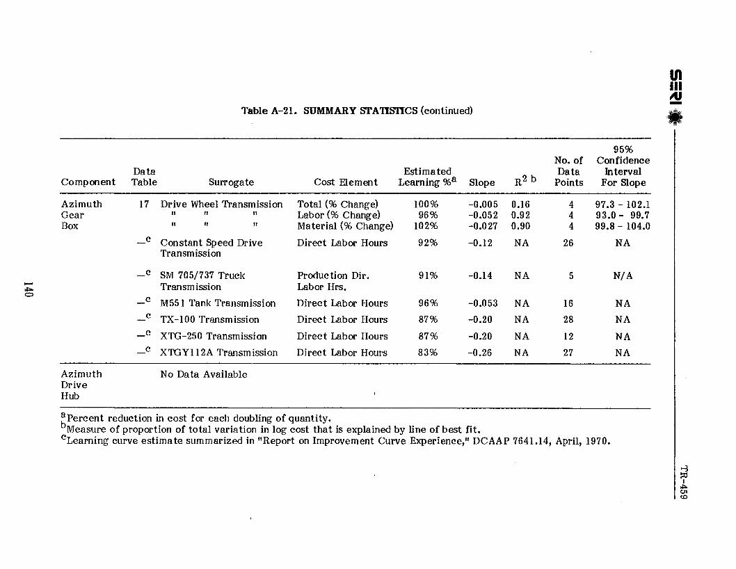
Table A-21. SUMMARY STATISTICS (continued)

95%No. of Confidence

Data EstimatedR2 b

Data IntervalComponent Table Surrogate Cost Element Learning %a Slope Points For Slope

Azimuth 17 Drive Wheel Transmission Total (% Change) 100% -0.005 0.16 4 97.3 - 102.1Gear " " " Labor (% Change) 96% -0.052 0.92 4 93.0 - 99.7Box " " " Material (% Change) 102% -0.027 0.90 4 99.8 - 104.0

- c Constant Speed Drive Direct Labor Hours 92% -0.12 NA 26 NATransmission

c SM 705/737 Truck Production Dir. 91% -0.14 NA 5 N/A..... Transm ission Labor Hrs,,;::..0

- c M551 Tank Transmission Direct Labor Hours 96% -0.053 NA 16 NA

- c TX- 100 Transm ission Direct Labor Hours 87% -0.20 NA 28 NA_c XTG-250 Transmission Direct Labor Hours 87% -0.20 NA 12 NA

- c XTGYl12A Transmission Direct Labor Hours 83% -0.26 NA 27 NA

Azimuth No Data AvailableDriveHub

a Percent reduction in cost for each doubling of quantity.bMeasure of proportion of total variation in log cost that is explained by line of best fit.cLearning curve estimate summarized in "Report on Improvement Curve Experience," DCAAP 7641.14, April, 1970.

IIIIIIN-

Table A-21. SUMMARY STATIS11CS (continued)

InIII~-

Data EstimatedComponent Table Surrogate Cost Element Learning %a

Reflector 18 Fabricated Piping and Fittings Labor $ (CUM) 98%Yoke 11 " n n Total $ (CUM) 99%

" 11 11 " Labor $ 98%fI 11 11 " Total $ 99%

95%No. of ConfidenceData Interval

Slope R2 b Points For Slope

-0.025 0.37 10 96.0 - 100.1-0.009 0.38 10 98.7-100.0-0.030 0.08 10 92.0 - 103.9-0.012 0.12 10 97.3 - 101.1

13 Steel Pipes and TubesData also given for Reflector Supports

...... 16 Metal Household Furniture;l::l.......

Reflector 19 Airc raft Canopy Labor Hours 68% -0.56 0.88 7 58.0 - 79.9Enclosure (Actual)

n " Labor Hours 81% -0.30 1.00 7 81.3 - 81.6(Adjusted)

20 Helicopter Blade Liners Labor $ 91% -0.14 0.99 4 88.1 - 94.1

" II n Total $ 86% -0.22 0.90 7 80.8 - 90.9_c Inflatable Shelter Labor Hours 85% -0.24 NA 10 NA

8Percent reduction in cost for each doubling of quantity.bMeasure of proportion of total variation in log cost that is explained by line of best fit.cLearning curve estimate summarized in "Report on Improvement Curve Experience," DCAAP 7641.14, April, 1970.

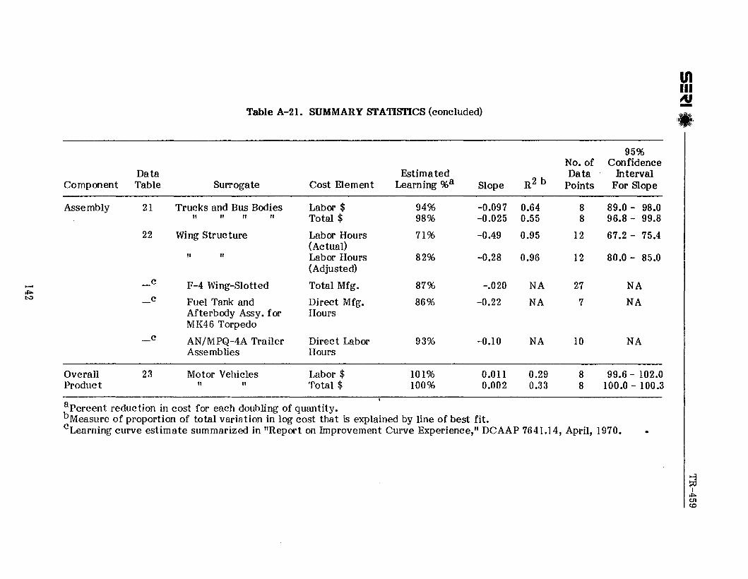
Table A-2l. SUMMARY STATISTICS (concluded)

95%No. of Confidence

Data Estimated Data IntervalComponent Table Surrogate Cost Element Learning %a Slope R2 b Points For Slope

Assembly 21 Trucks and Bus Bodies Labor $ 94% -0.097 0.64 8 89.0 - 98.0" " " " Total $ 98% -0.025 0.55 8 96.8 - 99.8

22 Wing Structure Labor Hours 71% -0.49 0.95 12 67.2 - 75.4(Actual)

" " Labor Hours 82% -0.28 0.96 12 80.0 - 85.0(Adjusted)

c F-4 Wing-Slotted Total Mfg. 87% -.020 NA 27 NA.....,.j:>.I:,:) c Fuel Tank and Direct Mfg. 86% -0.22 NA 7 NA-

Afterbody Assy. for HoursMK46 Torpedo

_c AN/MPQ-4A Trailer Direc t Labor 93% -0.10 NA 10 NAAssemblies Hours

Overall 23 Motor Vehicles Labor $ 101% 0.01l 0.29 8 99.6 - 102.0Product " " Total $ 100% 0.002 0.33 8 100.0 - 100.3.apercent reduction in cost for each doubling of quantity.bMeasure of proportion of total variation in log cost that is explained by line of best fit.cLearning curve estimate summarized in "Report on Improvement Curve Experience," DCAAP 7641.14, April, 1970.

IIIIIIAI-

I.;;;~I'-:: ~,/

TR-459S=~I ,(I}I -------------------------

APPENDIX B

ESTIMATIONS OF THE SURROGATE LEARNING CURVE

143

144

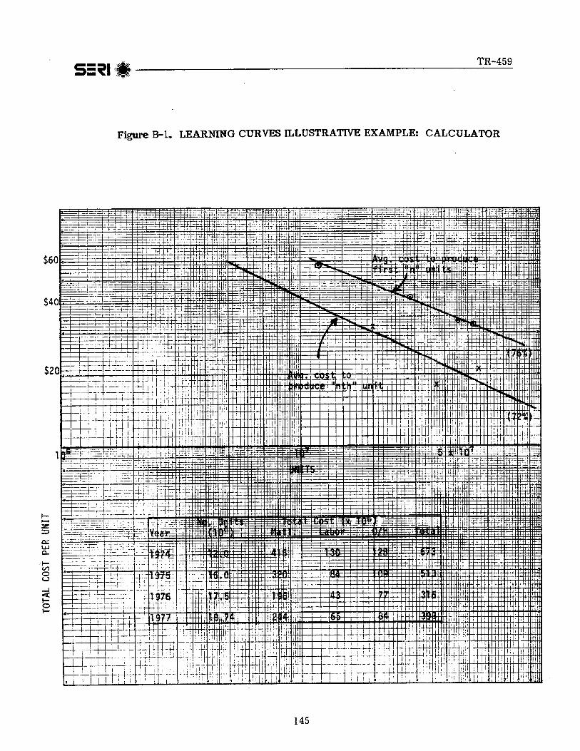
TR-459S=~II.I-------------------------

Figure B-1. LEARNING CURVES ILLUSTRATIVE EXAMPLE (continued)

(i) CUMULATIVE AVERAGE CURVE

PlotPoint Average Cost

12.0 673/12 = $56.0828.0 (673 + 513)/28 = $42.3645.5 (673 + 513 + 316)/45.5 = $33.0164.24 (673 + 513 + 316 + 393)/64.24 = $29.50

CD UN IT COST CURVE

PlotPoint* Unit Cost

5.3 673/12 = $56.0820.0 513/16 = $32.0636.7 316/17.5 = $18.0654.7 393/18.74 = $20.97

*Plot Point =(. ±: log i) /N1 = F

where F = first unit in lotL = last unit in lotN = number of units in lot

146

TR-459S=~I!.'----------------------

APPENDIX C

COST CURVES FOR THE MDAC AND GE HEIJOSTAT DESIGNS

151

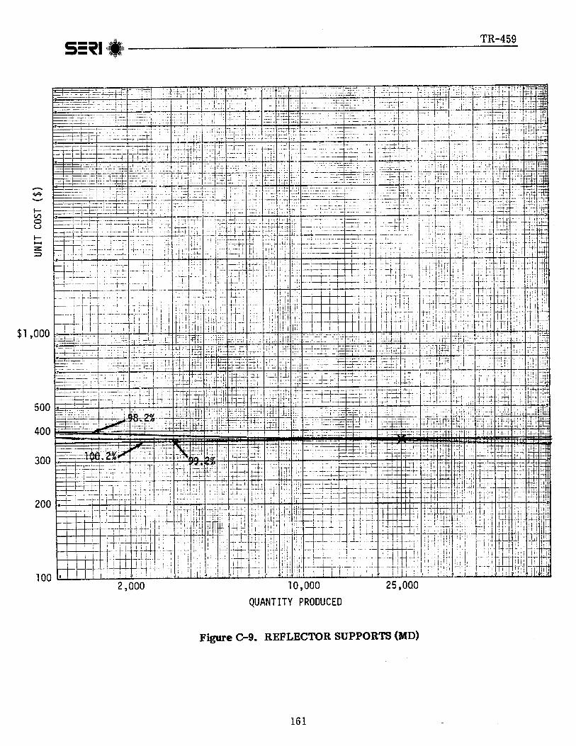
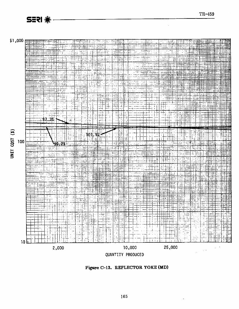
Document Control I" SERI Report No.

Page TR-353-4594. Title and Subtitle

12. NTIS Accession No. 3. Recipient's Accession No.

5. Publication Date

An Investigation of Learning and Experience Curves

7. Autnorts)

Kr;,n.ri Pro F' Th r-on r ori _ J.: Edesess .. M.9. Performing Organization Name and Address

Solar Energy Research Institute1617 Cole BoulevardGolden, Colorado 80401

12. Sponsoring Organization Name and Address

15. Supplementary Notes

Aori1 19806.

8. Performing Organization Rept. No.

10. Project/Task/Work Unit No.

522711. Contract (C) or Grant (G) No.

(C)

(G)

13. Type of Report & Perioa Covered

Technical Reoort14.

16. Abstract (Limit: 200 words)This study assesses the applicability of learning and experience curves for pre-dicting future costs of solar technologies, and the major test case is the pro­duction economics of heliostats. Alternative methods for estimating costreductions in systems manufacture are discussed, and procedures for using learn­ing and experience curves to predict costs are outlined. Because adequateproduction data often do not exist, production histories of analogous products/processes are analyzed and learning and aggregated cost curves for thesesurrogates estimated. If the surrogate learning curves apply, they can be usedto estimate solar technology costs. The steps involved in generating these costestimates are given. Second-generation glass-steel and inflated-bubble heliostatdesign concepts, developed by MDAC and GE, respectively, are described; a costingscenario for 25,000 units/yr is detailed; surrogates for cost analysis are chosen;learning and aggregate cost curves are estimated; and aggregate cost curves forthe GE and MDAC designs are estimated. However, an approach that combines aneoclassical production function with a learning-by-doing hypothesis is neededto yield a cost relation compatible with the historical learning curve and thetraditional cost function of economic theory.

17. Document Analvsis

a. Descriptors Learning Curves ; Exper ience Curves ; Comrnercializa tion ; Design ;Production ; Cost ; Learning ; Heliostats ; Installation

b. Identifiers/Open-Ended Terms

c. UC Cateqories

18. Avallaollity StatementNational Technical Information Serviceu. S. Department of Commerce5285 Port Royal RoadSpringfield, Virginia 22161

Form No. 8200-13 \6-79)

19. No. of Pages

19020. Price

$9.00