Propensity Score Matching Regression …...Propensity score matching An important attribute of PSM methods is that they do not require the functional form to be correctly speciﬁed

Propensity Score MatchingRegression Discontinuity

Limited Dependent Variables

Christopher F Baum

EC 823: Applied Econometrics

Boston College, Spring 2013

Christopher F Baum (BC / DIW) PSM, RD, LDV Boston College, Spring 2013 1 / 99

Propensity score matching


Policy evaluation seeks to determine the effectiveness of a particularintervention. In economic policy analysis, we rarely can work withexperimental data generated by purely random assignment of subjectsto the treatment and control groups. Random assignment, analogousto the ’randomized clinical trial’ in medicine, seeks to ensure thatparticipation in the intervention, or treatment, is the only differentiatingfactor between treatment and control units.

In non-experimental economic data, we observe whether subjectswere treated or not, but in the absence of random assignment, must beconcerned with differences between the treated and non-treated. Forinstance, do those individuals with higher aptitude self-select into a jobtraining program? If so, they are not similar to correspondingindividuals along that dimension, even though they may be similar inother aspects.



The key concern is that of similarity. How can we find individuals whoare similar on all observable characteristics in order to match treatedand non-treated individuals (or plants, or firms...) With a singlemeasure, we can readily compute a measure of distance between atreated unit and each candidate match. With multiple measuresdefining similarity, how are we to balance similarity along each of thosedimensions?

The method of propensity score matching (PSM) allows this matchingproblem to be reduced to a single dimension: that of the propensityscore. That score is defined as the probability that a unit in the fullsample receives the treatment, given a set of observed variables. If allinformation relevant to participation and outcomes is observable to theresearcher, the propensity score will produce valid matches forestimating the impact of an intervention. Thus, rather than matching onall values of the variables, individual units can be compared on thebasis of their propensity scores alone.



An important attribute of PSM methods is that they do not require thefunctional form to be correctly specified. If we used OLS methods suchas

y = Xβ + Dγ + ε

where y is the outcome, X are covariates and D is the treatmentindicator, we would be assuming that the effects of treatment areconstant across individuals. We need not make this assumption toemploy PSM. As we will see, a crucial assumption is made on thecontents of X , which should include all variables that can influence theprobability of treatment.


Propensity score matching Why use matching methods?

Why use matching methods?

The greatest challenge in evaluating a policy intervention is obtaining acredible estimate of the counterfactual: what would have happened toparticipants (treated units) had they not participated? Without acredible answer, we cannot rule out that whatever successes haveoccurred among participants could have happened anyway. Thisrelates to the fundamental problem of causal inference: it is impossibleto observe the outcomes of the same unit in both treatment conditionsat the same time.

The impact of a treatment on individual i , δi , is the difference betweenpotential outcomes with and without treatment:

δi = Y1i − Y0i

where states 0 and 1 corrrespond to non-treatment and treatment,respectively.



To evaluate the impact of a program over the population, we maycompute the average treatment effect (ATE):

ATE = E [δi ] = E(Y1 − Y0)

Most often, we want to compute the average treatment effect on thetreated (ATT):

ATT = E(Y1 − Y0|D = 1)

where D = 1 refers to the treatment.



The problem is that not all of these parameters are observable, as theyrely on counterfactual outcomes. For instance, we can rewrite ATT as

ATT = E(Y1|D = 1)− E(Y0|D = 1)

The second term is the average outcome of treated individuals hadthey not received the treatment. We cannot observe that, but we doobserve a corresponding quantity for the untreated, and can compute

∆ = E(Y1|D = 1)− E(Y0|D = 0)

The difference between ATT and ∆ can be defined as

∆ = ATT + SB

where SB is the selection bias term: the difference between thecounterfactual for treated units and observed outcomes for untreatedunits.



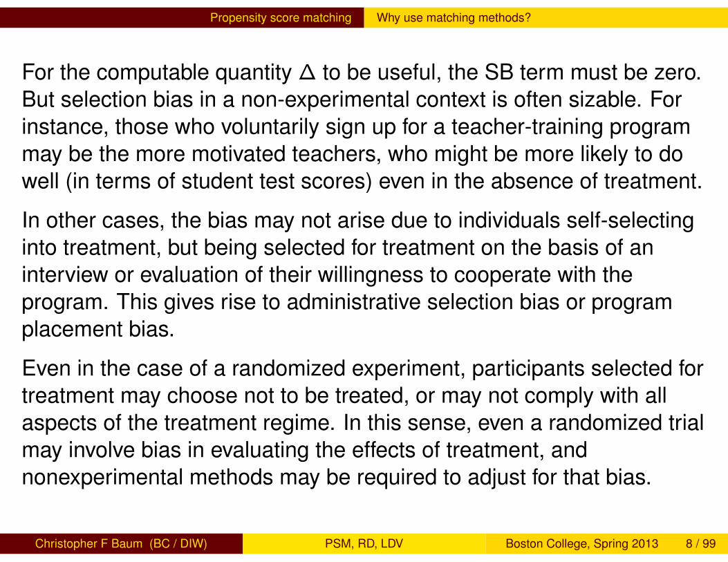
For the computable quantity ∆ to be useful, the SB term must be zero.But selection bias in a non-experimental context is often sizable. Forinstance, those who voluntarily sign up for a teacher-training programmay be the more motivated teachers, who might be more likely to dowell (in terms of student test scores) even in the absence of treatment.

In other cases, the bias may not arise due to individuals self-selectinginto treatment, but being selected for treatment on the basis of aninterview or evaluation of their willingness to cooperate with theprogram. This gives rise to administrative selection bias or programplacement bias.

Even in the case of a randomized experiment, participants selected fortreatment may choose not to be treated, or may not comply with allaspects of the treatment regime. In this sense, even a randomized trialmay involve bias in evaluating the effects of treatment, andnonexperimental methods may be required to adjust for that bias.


Propensity score matching Requirements for PSM validity

Requirements for PSM validity

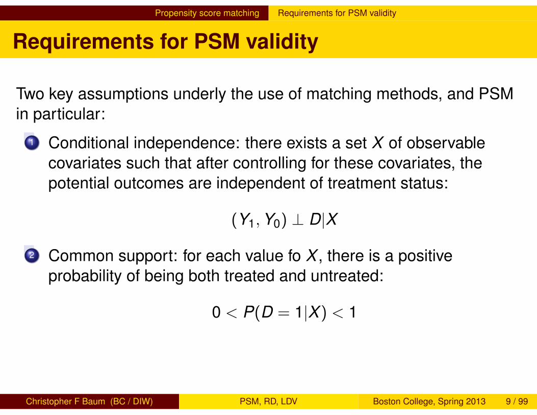
Two key assumptions underly the use of matching methods, and PSMin particular:

1 Conditional independence: there exists a set X of observablecovariates such that after controlling for these covariates, thepotential outcomes are independent of treatment status:

(Y1,Y0) ⊥ D|X

2 Common support: for each value fo X , there is a positiveprobability of being both treated and untreated:

0 < P(D = 1|X ) < 1



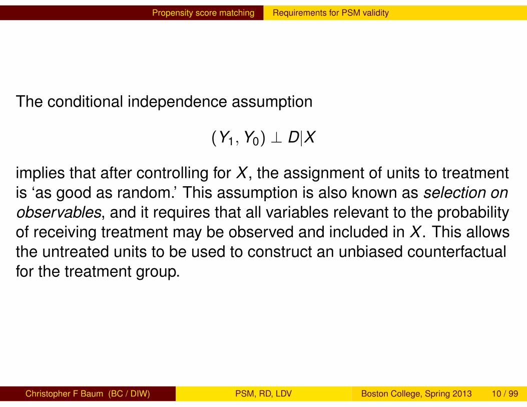
The conditional independence assumption

(Y1,Y0) ⊥ D|X

implies that after controlling for X , the assignment of units to treatmentis ‘as good as random.’ This assumption is also known as selection onobservables, and it requires that all variables relevant to the probabilityof receiving treatment may be observed and included in X . This allowsthe untreated units to be used to construct an unbiased counterfactualfor the treatment group.



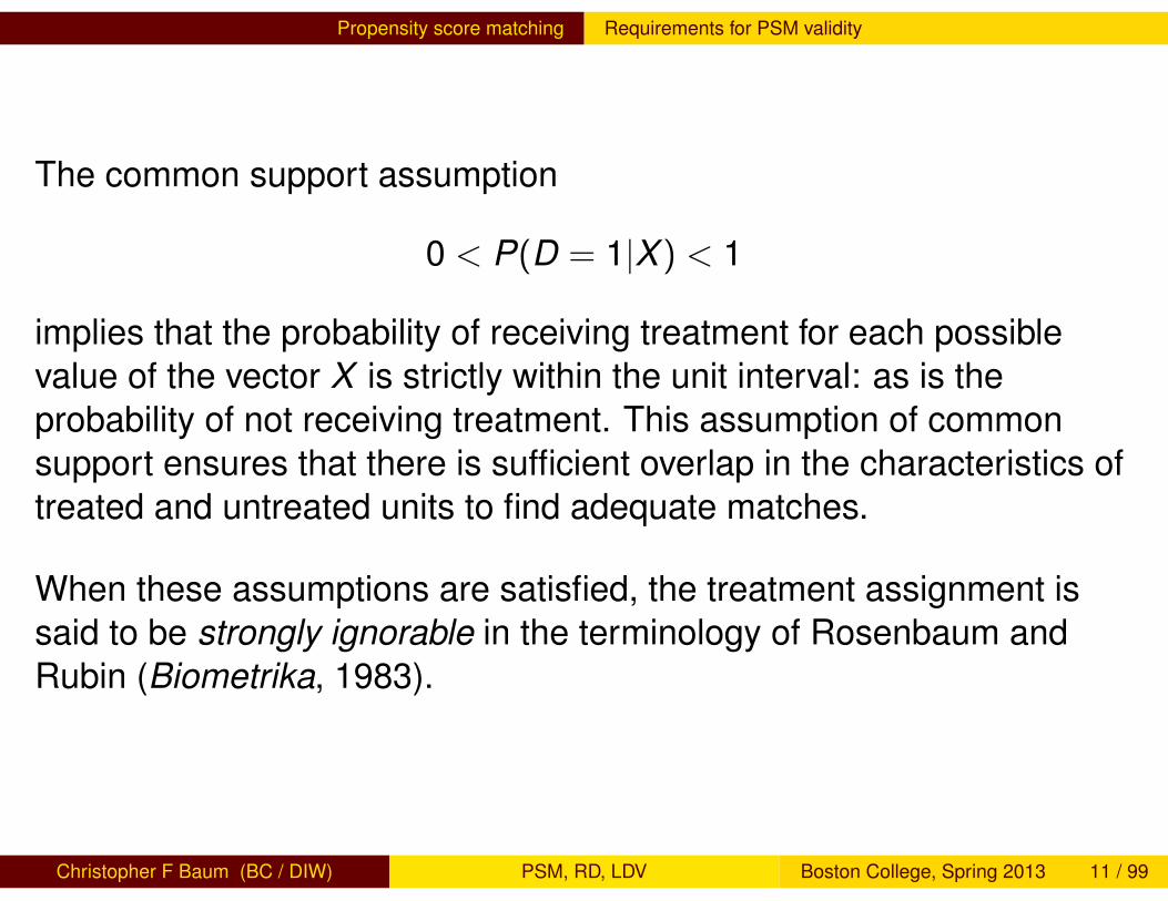
The common support assumption

0 < P(D = 1|X ) < 1

implies that the probability of receiving treatment for each possiblevalue of the vector X is strictly within the unit interval: as is theprobability of not receiving treatment. This assumption of commonsupport ensures that there is sufficient overlap in the characteristics oftreated and untreated units to find adequate matches.

When these assumptions are satisfied, the treatment assignment issaid to be strongly ignorable in the terminology of Rosenbaum andRubin (Biometrika, 1983).


Propensity score matching Basic mechanics of matching

Basic mechanics of matching

The procedure for estimating the impact of a program can be dividedinto three steps:

1 Estimate the propensity score2 Choose a matching algorithm that will use the estimated

propensity scores to match untreated units to treated units3 Estimate the impact of the intervention with the matched sample

and calculate standard errors



To estimate the propensity score, a logit or probit model is usuallyemployed. It is essential that a flexible functional form be used to allowfor possible nonlinearities in the participation model. This may involvethe introduction of higher-order terms in the covariates as well asinteraction terms.

There will usually be no comprehensive list of the clearly relevantvariables that would assure that the matched comparison group willprovide an unbiased estimate of program impact. Obviously explicitcriteria that govern project or program eligibility should be included, aswell as factors thought to influence self-selection and administrativeselection.



In choosing a matching algorithm, you must consider whethermatching is to be performed with or without replacement. Withoutreplacement, a given untreated unit can only be matched with onetreated unit. A criterion for assessing the quality of the match mustalso be defined. The number of untreated units to be matched witheach treated unit must also be chosen.

Early matching estimators paired each treated unit with one unit fromthe control group, judged most similar. Researchers have found thatestimators are more stable if a number of comparison cases areconsidered for each treated case, usually implying that the matchingwill be done with replacement.



The matching criterion could be as simple as the absolute difference inthe propensity score for treated vs. non-treated units. However, whenthe sampling design oversamples treated units, it has been found thatmatching on the log odds of the propensity score (p/(1− p)) is asuperior criterion.

The nearest neighbor matching algorithm merely evaluates absolutedifferences between propensity scores (or their log odds), where youmay choose to use 1, 2, ... K nearest neighbors in the match. Avariation, radius matching, specifies a ‘caliper’ or maximum propensityscore difference. Larger differences will not result in matches, and allunits whose differences lie within the caliper’s radius will be chosen.



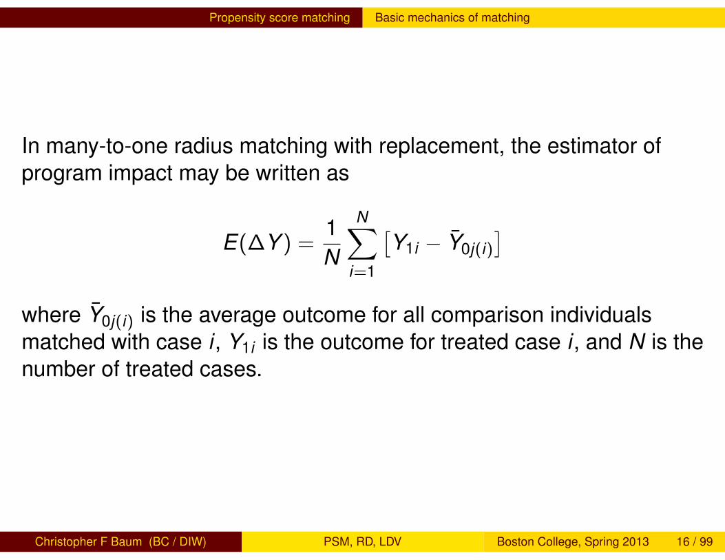
In many-to-one radius matching with replacement, the estimator ofprogram impact may be written as

E(∆Y ) =1N

N∑i=1

[Y1i − Y0j(i)

]where Y0j(i) is the average outcome for all comparison individualsmatched with case i , Y1i is the outcome for treated case i , and N is thenumber of treated cases.



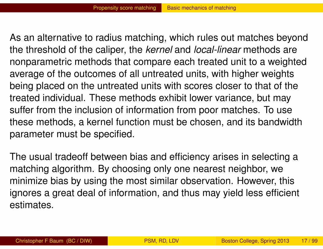
As an alternative to radius matching, which rules out matches beyondthe threshold of the caliper, the kernel and local-linear methods arenonparametric methods that compare each treated unit to a weightedaverage of the outcomes of all untreated units, with higher weightsbeing placed on the untreated units with scores closer to that of thetreated individual. These methods exhibit lower variance, but maysuffer from the inclusion of information from poor matches. To usethese methods, a kernel function must be chosen, and its bandwidthparameter must be specified.

The usual tradeoff between bias and efficiency arises in selecting amatching algorithm. By choosing only one nearest neighbor, weminimize bias by using the most similar observation. However, thisignores a great deal of information, and thus may yield less efficientestimates.


Propensity score matching Evaluating the validity of matching assumptions

Evaluating the validity of matching assumptions

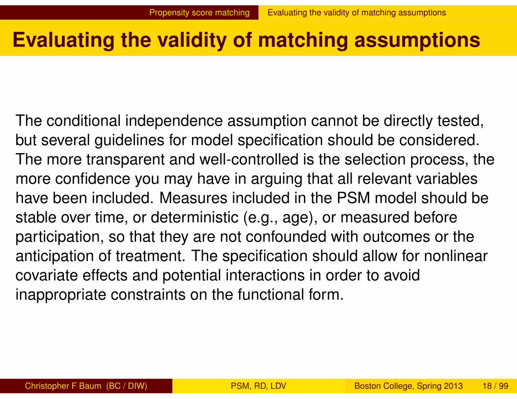
The conditional independence assumption cannot be directly tested,but several guidelines for model specification should be considered.The more transparent and well-controlled is the selection process, themore confidence you may have in arguing that all relevant variableshave been included. Measures included in the PSM model should bestable over time, or deterministic (e.g., age), or measured beforeparticipation, so that they are not confounded with outcomes or theanticipation of treatment. The specification should allow for nonlinearcovariate effects and potential interactions in order to avoidinappropriate constraints on the functional form.



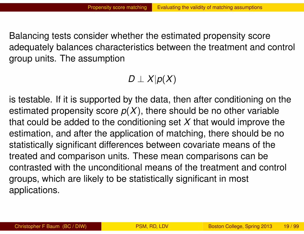
Balancing tests consider whether the estimated propensity scoreadequately balances characteristics between the treatment and controlgroup units. The assumption

D ⊥ X |p(X )

is testable. If it is supported by the data, then after conditioning on theestimated propensity score p(X ), there should be no other variablethat could be added to the conditioning set X that would improve theestimation, and after the application of matching, there should be nostatistically significant differences between covariate means of thetreated and comparison units. These mean comparisons can becontrasted with the unconditional means of the treatment and controlgroups, which are likely to be statistically significant in mostapplications.



Finally, the common support or overlap condition

0 < P(D = 1|X ) < 1

should be tested. This can be done by visual inspection of thedensities of propensity scores of treated and non-treated groups, ormore formally via a comparison test such as the Kolmogorov–Smirnovnonparametric test. If there are sizable differences between themaxima and minima of the density distributions, it may be advisable toremove cases that lie outside the support of the other distribution.However, as with any trimming algorithm, this implies that results of theanalysis are strictly valid only for the region of common support.


Propensity score matching An empirical example

An empirical example

As an example of propensity score matching techniques, we followSianesi’s 2010 presentation at the German Stata Users Groupmeetings (http://ideas.repec.org/p/boc/dsug10/02.html)and employ the nsw_psid dataset that has been used in severalarticles on PSM techniques. This dataset combines 297 treatedindividuals from a randomised evaluation of the NSW Demonstrationjob-training program with 2,490 non-experimental untreated individualsdrawn from the Panel Study of Income Dynamics (PSID), all of whomare male. The outcome of interest is re78, 1978 earnings. Availablecovariates include age, ethnic status (black, Hispanic or white), maritalstatus, years of education, an indicator for no high school degree and1975 earnings (in 1978 dollars).

We use Leuven and Sianesi’s psmatch2 routine, available from SSC.



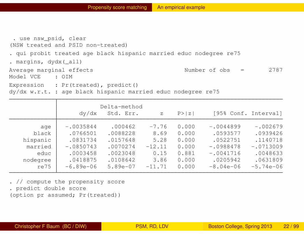
. use nsw_psid, clear(NSW treated and PSID non-treated)

. qui probit treated age black hispanic married educ nodegree re75

. margins, dydx(_all)

Average marginal effects Number of obs = 2787Model VCE : OIM

Expression : Pr(treated), predict()dy/dx w.r.t. : age black hispanic married educ nodegree re75

Delta-methoddy/dx Std. Err. z P>|z| [95% Conf. Interval]

age -.0035844 .000462 -7.76 0.000 -.0044899 -.002679black .0766501 .0088228 8.69 0.000 .0593577 .0939426

hispanic .0831734 .0157648 5.28 0.000 .0522751 .1140718married -.0850743 .0070274 -12.11 0.000 -.0988478 -.0713009

educ .0003458 .0023048 0.15 0.881 -.0041716 .0048633nodegree .0418875 .0108642 3.86 0.000 .0205942 .0631809

re75 -6.89e-06 5.89e-07 -11.71 0.000 -8.04e-06 -5.74e-06

. // compute the propensity score

. predict double score(option pr assumed; Pr(treated))



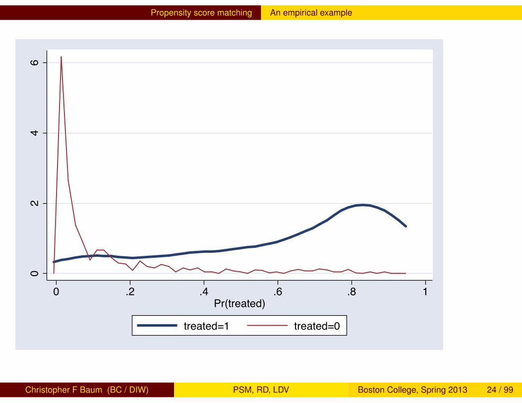
. // compare the densities of the estimated propensity score over groups. density2 score, group(treated) saving(psm2a, replace)(file psm2a.gph saved)

. graph export psm2a.pdf, replace(file /Users/cfbaum/Documents/Stata/StataWorkshops/psm2a.pdf written in PDF for> mat)

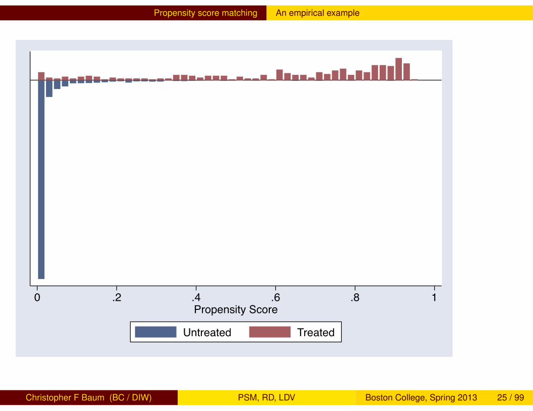
. psgraph, treated(treated) pscore(score) bin(50) saving(psm2b, replace)(file psm2b.gph saved)

. graph export psm2b.pdf, replace(file /Users/cfbaum/Documents/Stata/StataWorkshops/psm2b.pdf written in PDF for> mat)



02

46

0 .2 .4 .6 .8 1Pr(treated)

treated=1 treated=0



0 .2 .4 .6 .8 1Propensity Score

Untreated Treated



1 . // compute nearest-neighbor matching with caliper and replacement2 . psmatch2 treated, pscore(score) outcome(re78) caliper(0.01)There are observations with identical propensity score values.The sort order of the data could affect your results.Make sure that the sort order is random before calling psmatch2.

Variable Sample Treated Controls Difference S.E. T-stat

re78 Unmatched 5976.35202 21553.9209 -15577.5689 913.328457 -17.06 ATT 6067.8117 5768.70099 299.110712 1078.28065 0.28

Note: S.E. does not take into account that the propensity score is estimated.

psmatch2: psmatch2: Common Treatment supportassignment Off suppo On suppor Total

Untreated 0 2,490 2,490 Treated 26 271 297

Total 26 2,761 2,787

3 . // evaluate common support4 . summarize _support if treated

Variable Obs Mean Std. Dev. Min Max

_support 297 .9124579 .2831048 0 1

5 . qui log close

Monday, August 22, 2011 11:14 AM Page 1



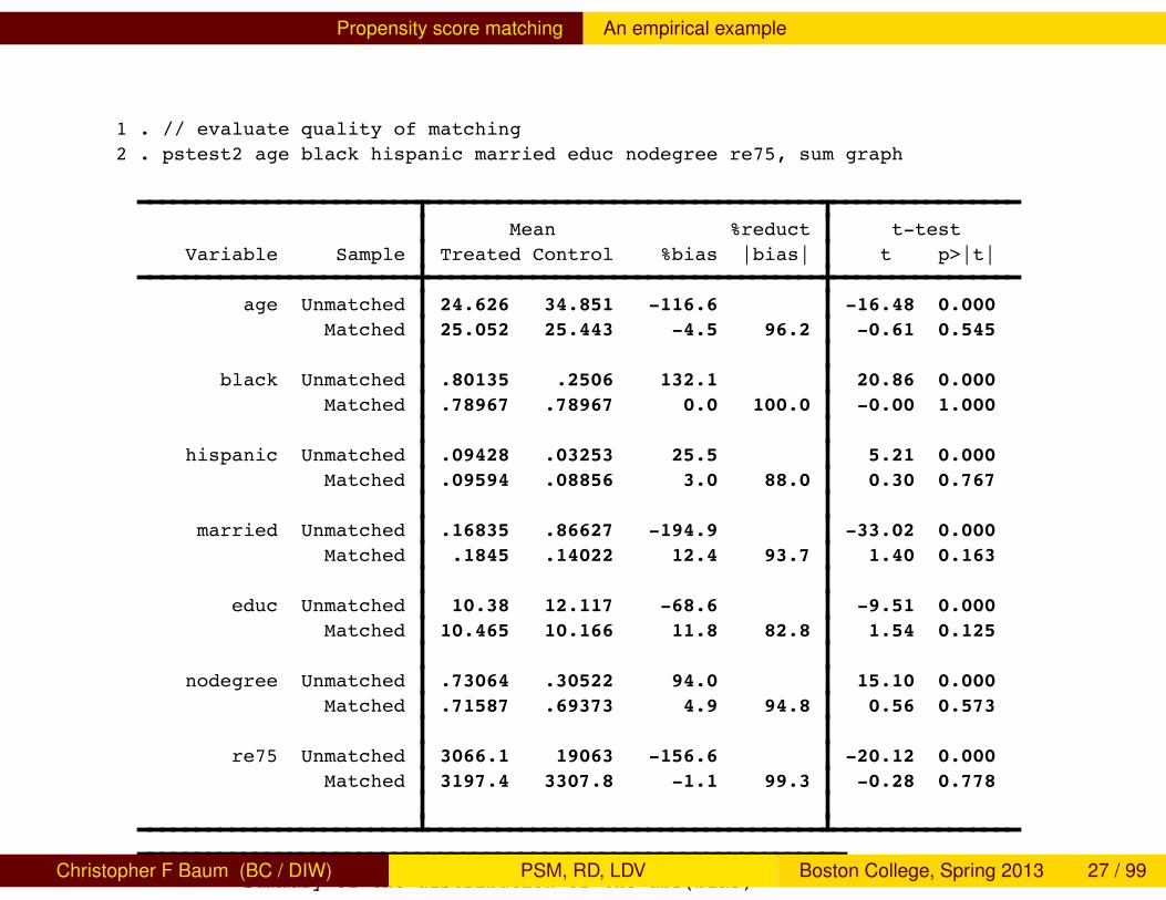
1 . // evaluate quality of matching2 . pstest2 age black hispanic married educ nodegree re75, sum graph

Mean %reduct t-test Variable Sample Treated Control %bias |bias| t p>|t|

age Unmatched 24.626 34.851 -116.6 -16.48 0.000 Matched 25.052 25.443 -4.5 96.2 -0.61 0.545 black Unmatched .80135 .2506 132.1 20.86 0.000 Matched .78967 .78967 0.0 100.0 -0.00 1.000 hispanic Unmatched .09428 .03253 25.5 5.21 0.000 Matched .09594 .08856 3.0 88.0 0.30 0.767 married Unmatched .16835 .86627 -194.9 -33.02 0.000 Matched .1845 .14022 12.4 93.7 1.40 0.163 educ Unmatched 10.38 12.117 -68.6 -9.51 0.000 Matched 10.465 10.166 11.8 82.8 1.54 0.125 nodegree Unmatched .73064 .30522 94.0 15.10 0.000 Matched .71587 .69373 4.9 94.8 0.56 0.573 re75 Unmatched 3066.1 19063 -156.6 -20.12 0.000 Matched 3197.4 3307.8 -1.1 99.3 -0.28 0.778

Summary of the distribution of the abs(bias)

BEFORE MATCHING

Percentiles Smallest 1% 25.51126 25.51126 5% 25.51126 68.622410% 25.51126 94.00328 Obs 725% 68.6224 116.6243 Sum of Wgt. 7




-200 -100 0 100 200

married

re75

age

educ

hispanic

nodegree

black

Unmatched Matched



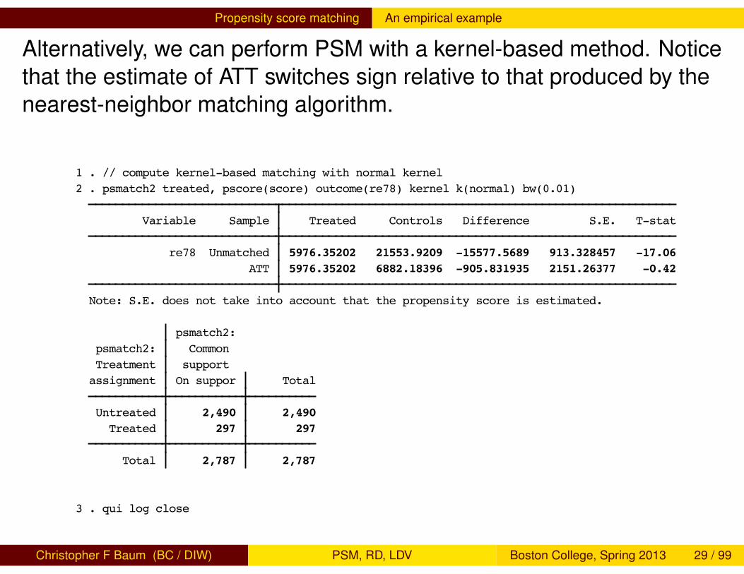
Alternatively, we can perform PSM with a kernel-based method. Noticethat the estimate of ATT switches sign relative to that produced by thenearest-neighbor matching algorithm.

1 . // compute kernel-based matching with normal kernel2 . psmatch2 treated, pscore(score) outcome(re78) kernel k(normal) bw(0.01)

Variable Sample Treated Controls Difference S.E. T-stat

re78 Unmatched 5976.35202 21553.9209 -15577.5689 913.328457 -17.06 ATT 5976.35202 6882.18396 -905.831935 2151.26377 -0.42

Note: S.E. does not take into account that the propensity score is estimated.

psmatch2: psmatch2: Common Treatment supportassignment On suppor Total

Untreated 2,490 2,490 Treated 297 297

Total 2,787 2,787

3 . qui log close




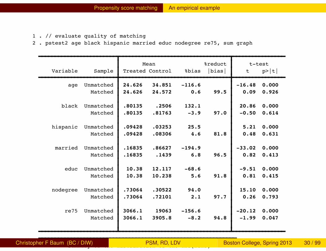
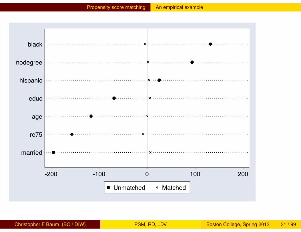
1 . // evaluate quality of matching2 . pstest2 age black hispanic married educ nodegree re75, sum graph

Mean %reduct t-test Variable Sample Treated Control %bias |bias| t p>|t|

age Unmatched 24.626 34.851 -116.6 -16.48 0.000 Matched 24.626 24.572 0.6 99.5 0.09 0.926 black Unmatched .80135 .2506 132.1 20.86 0.000 Matched .80135 .81763 -3.9 97.0 -0.50 0.614 hispanic Unmatched .09428 .03253 25.5 5.21 0.000 Matched .09428 .08306 4.6 81.8 0.48 0.631 married Unmatched .16835 .86627 -194.9 -33.02 0.000 Matched .16835 .1439 6.8 96.5 0.82 0.413 educ Unmatched 10.38 12.117 -68.6 -9.51 0.000 Matched 10.38 10.238 5.6 91.8 0.81 0.415 nodegree Unmatched .73064 .30522 94.0 15.10 0.000 Matched .73064 .72101 2.1 97.7 0.26 0.793 re75 Unmatched 3066.1 19063 -156.6 -20.12 0.000 Matched 3066.1 3905.8 -8.2 94.8 -1.99 0.047

Summary of the distribution of the abs(bias)

BEFORE MATCHING

Percentiles Smallest 1% 25.51126 25.51126 5% 25.51126 68.622410% 25.51126 94.00328 Obs 725% 68.6224 116.6243 Sum of Wgt. 7




-200 -100 0 100 200

married

re75

age

educ

hispanic

nodegree

black

Unmatched Matched



We could also employ Mahalanobis matching, which matches on thewhole vector of X values (and possibly the propensity score as well),using a different distance metric.

An additional important issue: how might we address unobservedheterogeneity, as we do in a panel data context with fixed effectsmodels? A differences-in-differences matching estimator (DID) hasbeen proposed, in which rather than evaluating the effect on theoutcome variable, you evaluate the effect on the change in theoutcome variable, before and after the intervention. Akin to DIDestimators in standard policy evaluation, this allows us to control forthe notion that there may be substantial unobserved differencesbetween treated and untreated units, relaxing the ‘selection onobservables’ assumption.


Regression discontinuity models


The idea of Regression Discontinuity (RD) design, due to Thistlewaiteand Campbell (J. Educ. Psych., 1960) and Hahn et al. (Econometrica,2001) is to use a discontinuity in the level of treatment related to someobservable to get a consistent estimate of the LATE: the local averagetreatment effect. This compares those just eligible for the treatment(above the threshold) to those just ineligible (below the threshold).

Among non-experimental or quasi-experimental methods, RDtechniques are considered to have the highest internal validity (theability to identify causal relationships in this research setting). Theirexternal validity (ability to generalize findings to similar contexts) maybe less impressive, as the estimated treatment effect is local to thediscontinuity.



What could give rise to a RD design? In 1996, a number of US statesadopted a policy that while immigrants were generally ineligible forfood stamps, a form of welfare assistance, those who had been in thecountry legally for at least five years would qualify. At a later date, onecould compare self-reported measures of dietary adequacy, ormeasures of obesity, between those immigrants who did and did notqualify for this assistance. The sharp discontinuity in this examplerelates to those on either side of the five-year boundary line.

Currently, US states are eligible for additional Federal funding if theirunemployment rate is above 8% (as most currently are). This fundingpermits UI recipients to receive a number of additional weeks ofbenefit. Two months ago, the Massachusetts unemployment ratedropped below the threshold: good news for those who are employed,but bad news for those still seeking a job, as the additional weeks ofbenefit are now not available to current recipients.



Other examples of RD designs arise in terms of taxation. In my homestate of Massachusetts, items of clothing are not taxable if they costless than US$250.00. An item selling for that price or higher is taxableat 6.25%. During a recent weekend ‘sales tax holiday’, itemspurchased on a single invoice were not taxable if the total was belowUS$2,500.00. Thus, a one-dollar increase in the invoice would incur anadditional US$156.25 in taxes, as the entire sale is then taxable.

As Austin Nichols pointed out, the sequence of US estate tax rates onlarge inheritances: 45% in 2009, zero in 2010, and 55% in 2011 mayhave caused some perverse incentives among potential heirs! Thatmay be a difficult hypothesis to test, though, without the assistance ofthe homicide squad.


Regression discontinuity models RD design elements

RD design elements

There are four crucial elements to a RD design:1 Treatment is not randomly assigned, but dependent at least in part

on an observable assignment variable Z .2 There is a discontinuity at some cutoff value of the assignment

variable in the level of treatment.3 Individuals cannot manipulate their status to affect whether they

fall on one side of the cutoff or the other. Those near the cutoff areassumed to be exchangeable or otherwise identical.

4 Other variables are smooth functions of the assignment variable,conditional on treatment. That is, a jump in the outcome variableshould be due to the discontinuity in the level of treatment.


Regression discontinuity models RD methodology

RD methodology

There is considerable art involved in choosing some continuousfunction of the assignment variable Z for treatment and outcomes. Ahigh-order polynomial in Z is often used to estimate separately on bothsides of the discontinuity. Better yet, a local polynomial, local linearregression model or local mean smoother may be used, where as inother nonparametric settings one must choose a kernel and bandwidthparameter. It is probably best to choose several different bandwidthparameters to analyze the sensitivity of the results to the choice ofbandwidth.


Regression discontinuity models RD methodology

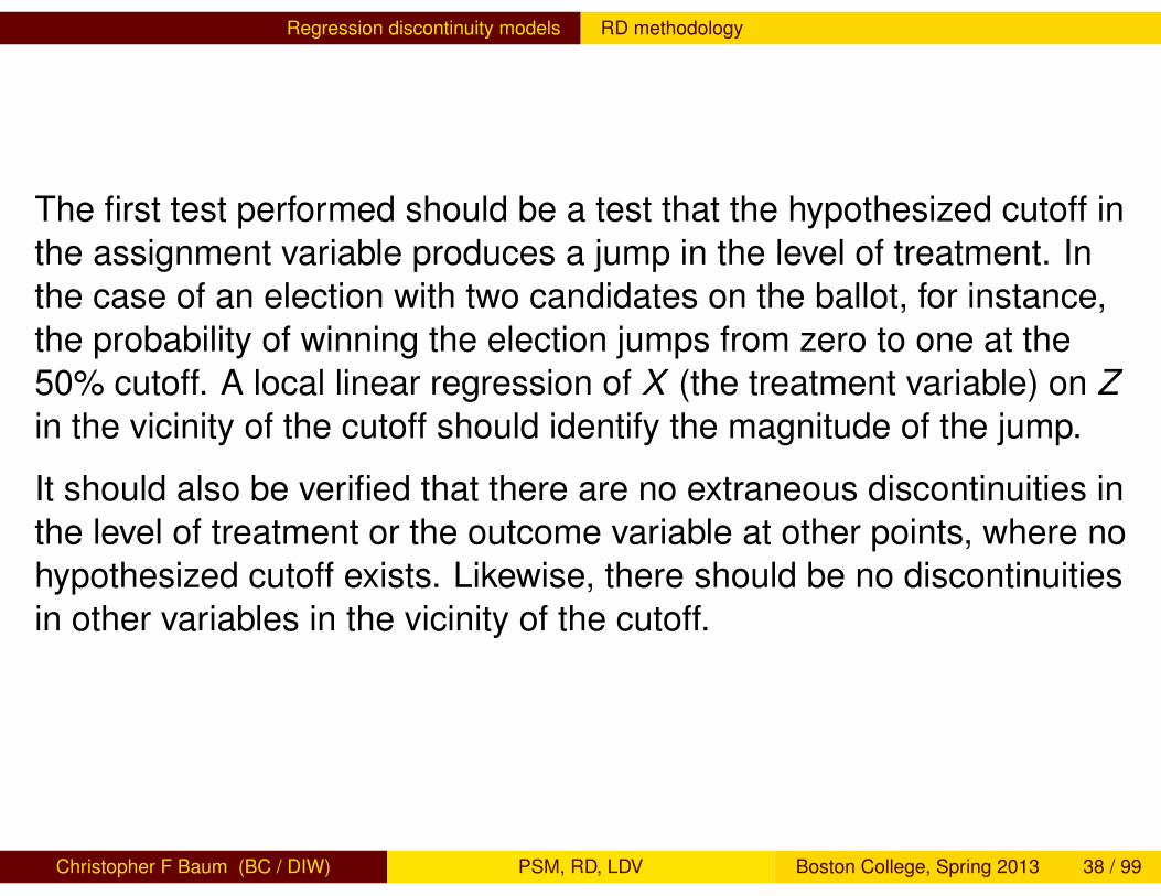
The first test performed should be a test that the hypothesized cutoff inthe assignment variable produces a jump in the level of treatment. Inthe case of an election with two candidates on the ballot, for instance,the probability of winning the election jumps from zero to one at the50% cutoff. A local linear regression of X (the treatment variable) on Zin the vicinity of the cutoff should identify the magnitude of the jump.

It should also be verified that there are no extraneous discontinuities inthe level of treatment or the outcome variable at other points, where nohypothesized cutoff exists. Likewise, there should be no discontinuitiesin other variables in the vicinity of the cutoff.


Regression discontinuity models RD empirical example

RD empirical example

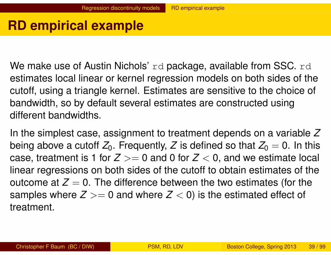
We make use of Austin Nichols’ rd package, available from SSC. rdestimates local linear or kernel regression models on both sides of thecutoff, using a triangle kernel. Estimates are sensitive to the choice ofbandwidth, so by default several estimates are constructed usingdifferent bandwidths.

In the simplest case, assignment to treatment depends on a variable Zbeing above a cutoff Z0. Frequently, Z is defined so that Z0 = 0. In thiscase, treatment is 1 for Z >= 0 and 0 for Z < 0, and we estimate locallinear regressions on both sides of the cutoff to obtain estimates of theoutcome at Z = 0. The difference between the two estimates (for thesamples where Z >= 0 and where Z < 0) is the estimated effect oftreatment.



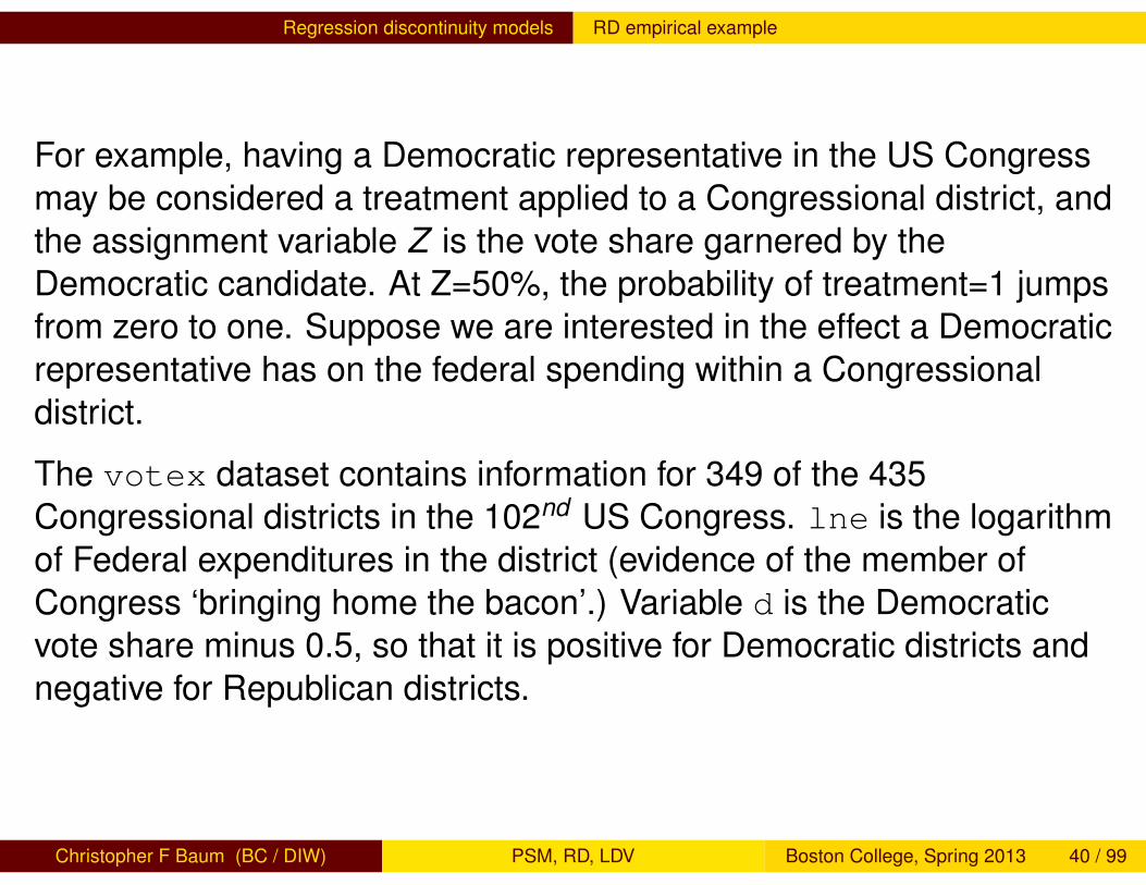
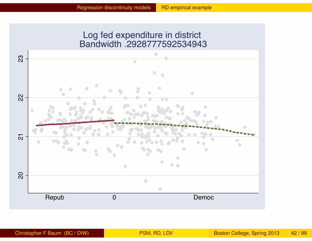
For example, having a Democratic representative in the US Congressmay be considered a treatment applied to a Congressional district, andthe assignment variable Z is the vote share garnered by theDemocratic candidate. At Z=50%, the probability of treatment=1 jumpsfrom zero to one. Suppose we are interested in the effect a Democraticrepresentative has on the federal spending within a Congressionaldistrict.

The votex dataset contains information for 349 of the 435Congressional districts in the 102nd US Congress. lne is the logarithmof Federal expenditures in the district (evidence of the member ofCongress ‘bringing home the bacon’.) Variable d is the Democraticvote share minus 0.5, so that it is positive for Democratic districts andnegative for Republican districts.



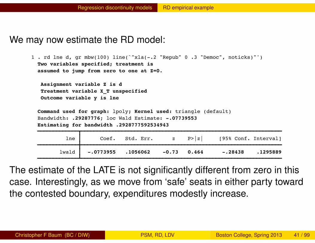
We may now estimate the RD model:

1 . rd lne d, gr mbw(100) line(`"xla(-.2 "Repub" 0 .3 "Democ", noticks)"')Two variables specified; treatment is assumed to jump from zero to one at Z=0.

Assignment variable Z is d Treatment variable X_T unspecified Outcome variable y is lne

Command used for graph: lpoly; Kernel used: triangle (default)Bandwidth: .29287776; loc Wald Estimate: -.07739553Estimating for bandwidth .2928777592534943

lne Coef. Std. Err. z P>|z| [95% Conf. Interval]

lwald -.0773955 .1056062 -0.73 0.464 -.28438 .1295889

2 . qui log close

Monday, August 22, 2011 4:16 PM Page 1

The estimate of the LATE is not significantly different from zero in thiscase. Interestingly, as we move from ‘safe’ seats in either party towardthe contested boundary, expenditures modestly increase.



2021

2223

Repub 0 Democ

Log fed expenditure in district Bandwidth .2928777592534943



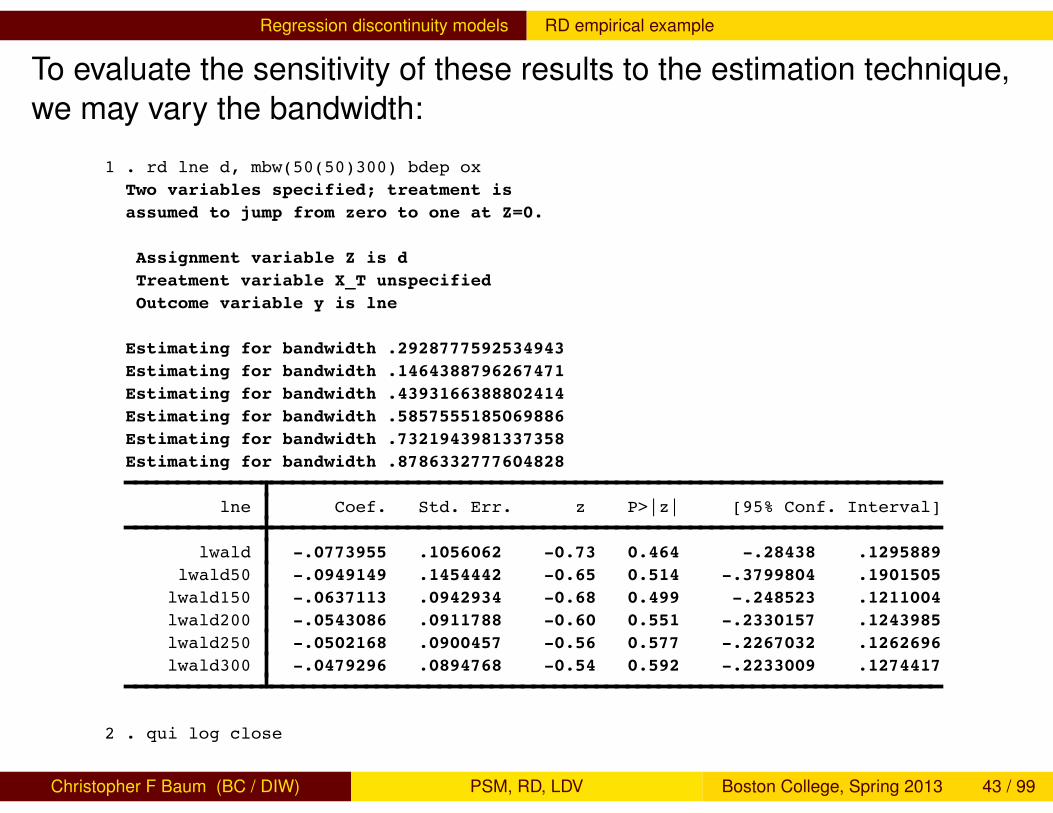
To evaluate the sensitivity of these results to the estimation technique,we may vary the bandwidth:

1 . rd lne d, mbw(50(50)300) bdep oxTwo variables specified; treatment is assumed to jump from zero to one at Z=0.

Assignment variable Z is d Treatment variable X_T unspecified Outcome variable y is lne

Estimating for bandwidth .2928777592534943Estimating for bandwidth .1464388796267471Estimating for bandwidth .4393166388802414Estimating for bandwidth .5857555185069886Estimating for bandwidth .7321943981337358Estimating for bandwidth .8786332777604828

lne Coef. Std. Err. z P>|z| [95% Conf. Interval]

lwald -.0773955 .1056062 -0.73 0.464 -.28438 .1295889 lwald50 -.0949149 .1454442 -0.65 0.514 -.3799804 .1901505 lwald150 -.0637113 .0942934 -0.68 0.499 -.248523 .1211004 lwald200 -.0543086 .0911788 -0.60 0.551 -.2330157 .1243985 lwald250 -.0502168 .0900457 -0.56 0.577 -.2267032 .1262696 lwald300 -.0479296 .0894768 -0.54 0.592 -.2233009 .1274417

2 . qui log close

Monday, August 22, 2011 4:17 PM Page 1



-.4-.2

0.2

Estim

ated

effe

ct

.29 .15 .44 .59 .73 .88Bandwidth

CI Est



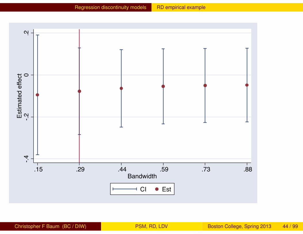
As we can see, the conclusion of no meaningful difference in theoutcome variable is not sensitive to the choice of bandwidth in the locallinear regression estimator.

For a more detailed discussion of RD and other quasi-experimentalmethods, see Austin Nichols, 2007, ‘Causal Inference withObservational Data,’ Stata Journal 7(4): 507–541. Freelydownloadable from http://www.stata-journal.com.


Limited dependent variables


We consider models of limited dependent variables in which theeconomic agent’s response is limited in some way. The dependentvariable, rather than being continuous on the real line (or half–line), isrestricted. In some cases, we are dealing with discrete choice: theresponse variable may be restricted to a Boolean or binary choice,indicating that a particular course of action was or was not selected.

In others, it may take on only integer values, such as the number ofchildren per family, or the ordered values on a Likert scale.Alternatively, it may appear to be a continuous variable with a numberof responses at a threshold value. For instance, the response to thequestion “how many hours did you work last week?" will be recordedas zero for the non-working respondents. None of these measures areamenable to being modeled by the linear regression methods we havediscussed.



We first consider models of Boolean response variables, or binarychoice. In such a model, the response variable is coded as 1 or 0,corresponding to responses of True or False to a particular question. Abehavioral model of this decision could be developed, including anumber of “explanatory factors” (we should not call them regressors)that we expect will influence the respondent’s answer to such aquestion. But we should readily spot the flaw in the linear probabilitymodel:

Ri = β1 + β2Xi2 + · · ·+ βkXik + ui (1)

where we place the Boolean response variable in R and regress itupon a set of X variables. All of the observations we have on R areeither 0 or 1. They may be viewed as the ex post probabilities ofresponding “yes” to the question posed. But the predictions of a linearregression model are unbounded, and the model of Equation (1),estimated with regress, can produce negative predictions andpredictions exceeding unity, neither of which can be consideredprobabilities.



Because the response variable is bounded, restricted to take on valuesof {0,1}, the model should be generating a predicted probability thatindividual i will choose to answer Yes rather than No. In such aframework, if βj > 0, those individuals with high values of Xj will bemore likely to respond Yes, but their probability of doing so mustrespect the upper bound.

For instance, if higher disposable income makes new car purchasemore probable, we must be able to include a very wealthy person inthe sample and still find that the individual’s predicted probability ofnew car purchase is no greater than 1.0. Likewise, a poor person’spredicted probability must be bounded by 0.


Limited dependent variables The latent variable approach

A useful approach to motivate such a model is that of a latent variable.Express the model of Equation (1) as:

y∗i = β1 + β2Xi2 + · · ·+ βkXik + ui (2)

where y∗ is an unobservable magnitude which can be considered thenet benefit to individual i of taking a particular course of action (e.g.,purchasing a new car). We cannot observe that net benefit, but canobserve the outcome of the individual having followed the decision rule

yi = 0 if y∗i < 0yi = 1 if y∗i ≥ 0 (3)



That is, we observe that the individual did or did not purchase a newcar in 2005. If she did, we observed yi = 1, and we take this asevidence that a rational consumer made a decision that improved herwelfare. We speak of y∗ as a latent variable, linearly related to a set offactors X and a disturbance process u.

In the latent variable model, we must make the assumption that thedisturbance process has a known variance σ2

u. Unlike the regressionproblem, we do not have sufficient information in the data to estimateits magnitude. Since we may divide Equation (2) by any positive σwithout altering the estimation problem, the most useful strategy is toset σu = σ2

u = 1.



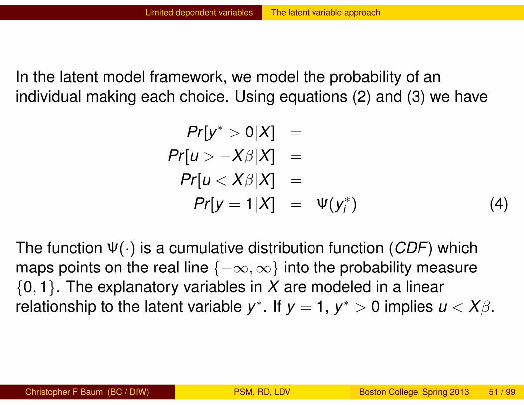
In the latent model framework, we model the probability of anindividual making each choice. Using equations (2) and (3) we have

Pr [y∗ > 0|X ] =

Pr [u > −Xβ|X ] =

Pr [u < Xβ|X ] =

Pr [y = 1|X ] = Ψ(y∗i ) (4)

The function Ψ(·) is a cumulative distribution function (CDF ) whichmaps points on the real line {−∞,∞} into the probability measure{0,1}. The explanatory variables in X are modeled in a linearrelationship to the latent variable y∗. If y = 1, y∗ > 0 implies u < Xβ.



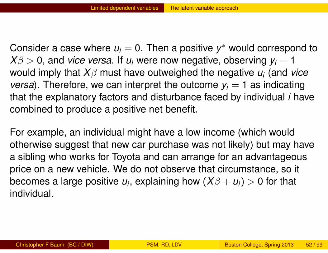
Consider a case where ui = 0. Then a positive y∗ would correspond toXβ > 0, and vice versa. If ui were now negative, observing yi = 1would imply that Xβ must have outweighed the negative ui (and viceversa). Therefore, we can interpret the outcome yi = 1 as indicatingthat the explanatory factors and disturbance faced by individual i havecombined to produce a positive net benefit.

For example, an individual might have a low income (which wouldotherwise suggest that new car purchase was not likely) but may havea sibling who works for Toyota and can arrange for an advantageousprice on a new vehicle. We do not observe that circumstance, so itbecomes a large positive ui , explaining how (Xβ + ui) > 0 for thatindividual.


Limited dependent variables Binomial probit and logit

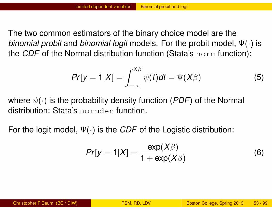
The two common estimators of the binary choice model are thebinomial probit and binomial logit models. For the probit model, Ψ(·) isthe CDF of the Normal distribution function (Stata’s norm function):

Pr [y = 1|X ] =

∫ Xβ

−∞ψ(t)dt = Ψ(Xβ) (5)

where ψ(·) is the probability density function (PDF ) of the Normaldistribution: Stata’s normden function.

For the logit model, Ψ(·) is the CDF of the Logistic distribution:

Pr [y = 1|X ] =exp(Xβ)

1 + exp(Xβ)(6)



The two models will produce quite similar results if the distribution ofsample values of yi is not too extreme. However, a sample in which theproportion yi = 1 (or the proportion yi = 0) is very small will besensitive to the choice of CDF . Neither of these cases are reallyamenable to the binary choice model.

If a very unusual event is being modeled by yi , the “naïve model” that itwill not happen in any event is hard to beat. The same is true for anevent that is almost ubiquitous: the naïve model that predicts thateveryone has eaten a candy bar at some time in their lives is quiteaccurate.



We may estimate these binary choice models in Stata with thecommands probit and logit, respectively. Both commands assumethat the response variable is coded with zeros indicating a negativeoutcome and a positive, non-missing value corresponding to a positiveoutcome (i.e., I purchased a new car in 2005). These commands donot require that the variable be coded {0,1}, although that is often thecase.

Because any positive value (including all missing values) will be takenas a positive outcome, it is important to ensure that missing values ofthe response variable are excluded from the estimation sample eitherby dropping those observations or using anif !mi( depvar ) qualifier.


Limited dependent variables Marginal effects and predictions

One of the major challenges in working with limited dependent variablemodels is the complexity of explanatory factors’ marginal effects on theresult of interest. That complexity arises from the nonlinearity of therelationship. In Equation (4), the latent measure is translated by Ψ(y∗i )to a probability that yi = 1. While Equation (2) is a linear relationship inthe β parameters, Equation (4) is not. Therefore, although Xj has alinear effect on y∗i , it will not have a linear effect on the resultingprobability that y = 1:

∂Pr [y = 1|X ]

∂Xj=∂Pr [y = 1|X ]

∂Xβ· ∂Xβ∂Xj

=

Ψ′(Xβ) · βj = ψ(Xβ) · βj .

The probability that yi = 1 is not constant over the data. Via the chainrule, we see that the effect of an increase in Xj on the probability is theproduct of two factors: the effect of Xj on the latent variable and thederivative of the CDF evaluated at y∗i . The latter term, ψ(·), is theprobability density function (PDF ) of the distribution.



In a binary choice model, the marginal effect of an increase in factor Xjcannot have a constant effect on the conditional probability that(y = 1|X ) since Ψ(·) varies through the range of X values. In a linearregression model, the coefficient βj and its estimate bj measures themarginal effect ∂y/∂Xj , and that effect is constant for all values of X .In a binary choice model, where the probability that yi = 1 is boundedby the {0,1} interval, the marginal effect must vary.

For instance, the marginal effect of a one dollar increase in disposableincome on the conditional probability that (y = 1|X ) must approachzero as Xj increases. Therefore, the marginal effect in such a modelvaries continuously throughout the range of Xj , and must approachzero for both very low and very high levels of Xj .



When using Stata’s probit (or logit) command, the reportedcoefficients (computed via maximum likelihood) are b, correspondingto β. You can use margins to compute the marginal effects. If aprobit estimation is followed by the command margins,dydx(_all), the dF/dx values will be calculated.

The margins command’s at() option can be used to compute theeffects at a particular point in the sample space. The marginscommand may also be used to calculate elasticities andsemi-elasticities.



After estimating a probit model, the predict command may be used,with a default option p, the predicted probability of a positive outcome.The xb option may be used to calculate the index function for eachobservation: that is, the predicted value of y∗i from Equation (4), whichis in z-units (those of a standard Normal variable). For instance, anindex function value of 1.69 will be associated with a predictedprobability of 0.95 in a large sample.



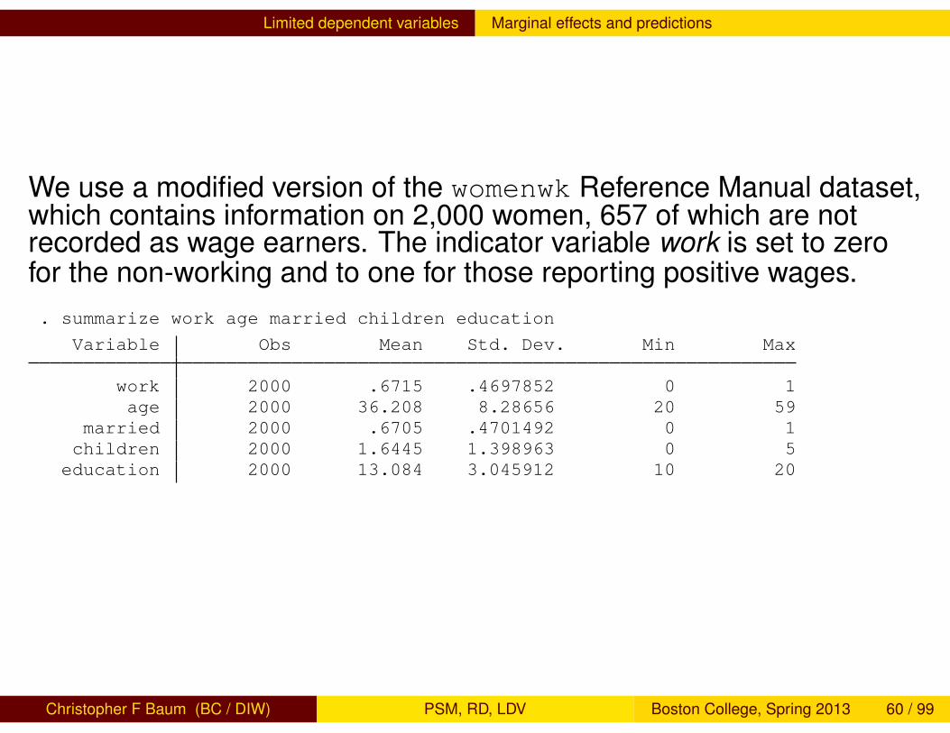
We use a modified version of the womenwk Reference Manual dataset,which contains information on 2,000 women, 657 of which are notrecorded as wage earners. The indicator variable work is set to zerofor the non-working and to one for those reporting positive wages.. summarize work age married children education


work 2000 .6715 .4697852 0 1age 2000 36.208 8.28656 20 59

married 2000 .6705 .4701492 0 1children 2000 1.6445 1.398963 0 5education 2000 13.084 3.045912 10 20



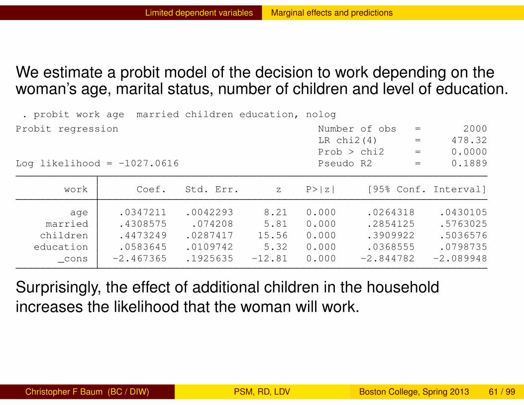
We estimate a probit model of the decision to work depending on thewoman’s age, marital status, number of children and level of education.. probit work age married children education, nolog

Probit regression Number of obs = 2000LR chi2(4) = 478.32Prob > chi2 = 0.0000

Log likelihood = -1027.0616 Pseudo R2 = 0.1889

work Coef. Std. Err. z P>|z| [95% Conf. Interval]

age .0347211 .0042293 8.21 0.000 .0264318 .0430105married .4308575 .074208 5.81 0.000 .2854125 .5763025

children .4473249 .0287417 15.56 0.000 .3909922 .5036576education .0583645 .0109742 5.32 0.000 .0368555 .0798735

_cons -2.467365 .1925635 -12.81 0.000 -2.844782 -2.089948

Surprisingly, the effect of additional children in the householdincreases the likelihood that the woman will work.



Average marginal effects (AMEs) are computed via margins.

. margins, dydx(_all)


Expression : Pr(work), predict()dy/dx w.r.t. : age married children education


age .0100768 .0011647 8.65 0.000 .0077941 .0123595married .1250441 .0210541 5.94 0.000 .0837788 .1663094


The marginal effects imply that married women have a 12.5% higherprobability of labor force participation, while the addition of a child isassociated with an 13% increase in participation.


Limited dependent variables Estimation with proportions data

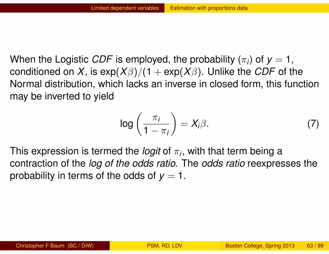
When the Logistic CDF is employed, the probability (πi ) of y = 1,conditioned on X , is exp(Xβ)/(1 + exp(Xβ). Unlike the CDF of theNormal distribution, which lacks an inverse in closed form, this functionmay be inverted to yield

log(

πi

1− πi

)= Xiβ. (7)

This expression is termed the logit of πi , with that term being acontraction of the log of the odds ratio. The odds ratio reexpresses theprobability in terms of the odds of y = 1.



As the logit of πi = Xiβ, it follows that the odds ratio for a one-unitchange in the j thX , holding other X constant, is merely exp(βj). Whenwe estimate a logit model, the or option specifies that odds ratiosare to be displayed rather than coefficients.

If the odds ratio exceeds unity, an increase in that X increases thelikelihood that y = 1, and vice versa. Estimated standard errors for theodds ratios are calculated via the delta method.



We can define the logit, or log of the odds ratio, in terms of groupeddata (averages of microdata). For instance, in the 2004 U.S.presidential election, the ex post probability of a Massachusettsresident voting for John Kerry was 0.62, with a logit oflog (0.62/(1− 0.62)) = 0.4895. The probability of that person votingfor George Bush was 0.37, with a logit of −0.5322. Say that we hadsuch data for all 50 states. It would be inappropriate to use linearregression on the probabilities voteKerry and voteBush, just as it wouldbe inappropriate to run a regression on individual voter’s voteKerry andvoteBush indicator variables.



In this case, Stata’s glogit (grouped logit) command may be used toproduce weighted least squares estimates for the model on state-leveldata. Alternatively, the blogit command may be used to producemaximum-likelihood estimates of that model on grouped (or “blocked”)data.

The equivalent commands gprobit and bprobit may be used to fita probit model to grouped data.


Limited dependent variables Ordered logit and probit models

Estimation with ordinal data

We earlier discussed the issues related to the use of ordinal variables:those which indicate a ranking of responses, rather than a cardinalmeasure, such as the codes of a Likert scale of agreement with astatement. Since the values of such an ordered response are arbitrary,an ordinal variable should not be treated as if it was measurable in acardinal sense and entered into a regression, either as a responsevariable or as a regressor.

However, what if we want to model an ordinal variable as the responsevariable, given a set of explanatory factors? Just as we can use binarychoice models to evaluate the factors underlying a decision withoutbeing able to quantify the net benefit of making that choice, we mayemploy a generalization of the binary choice framework to model anordinal variable using ordered probit or ordered logit estimationtechniques.



In the latent variable approach to the binary choice model, we observeyi = 1 if the individual’s net benefit is positive: i.e., y∗i > 0. The orderedchoice model generalizes this concept to the notion of multiplethresholds. For instance, a variable recorded on a five-point Likertscale will have four thresholds. If y∗ ≤ κ1, we observe y = 1. Ifκ1 < y∗ ≤ κ2, we observe y = 2. If κ2 < y∗ ≤ κ3, we observe y = 3,and so on, where the κ values are the thresholds. In a sense, this canbe considered imprecise measurement: we cannot observe y∗ directly,but only the range in which it falls.



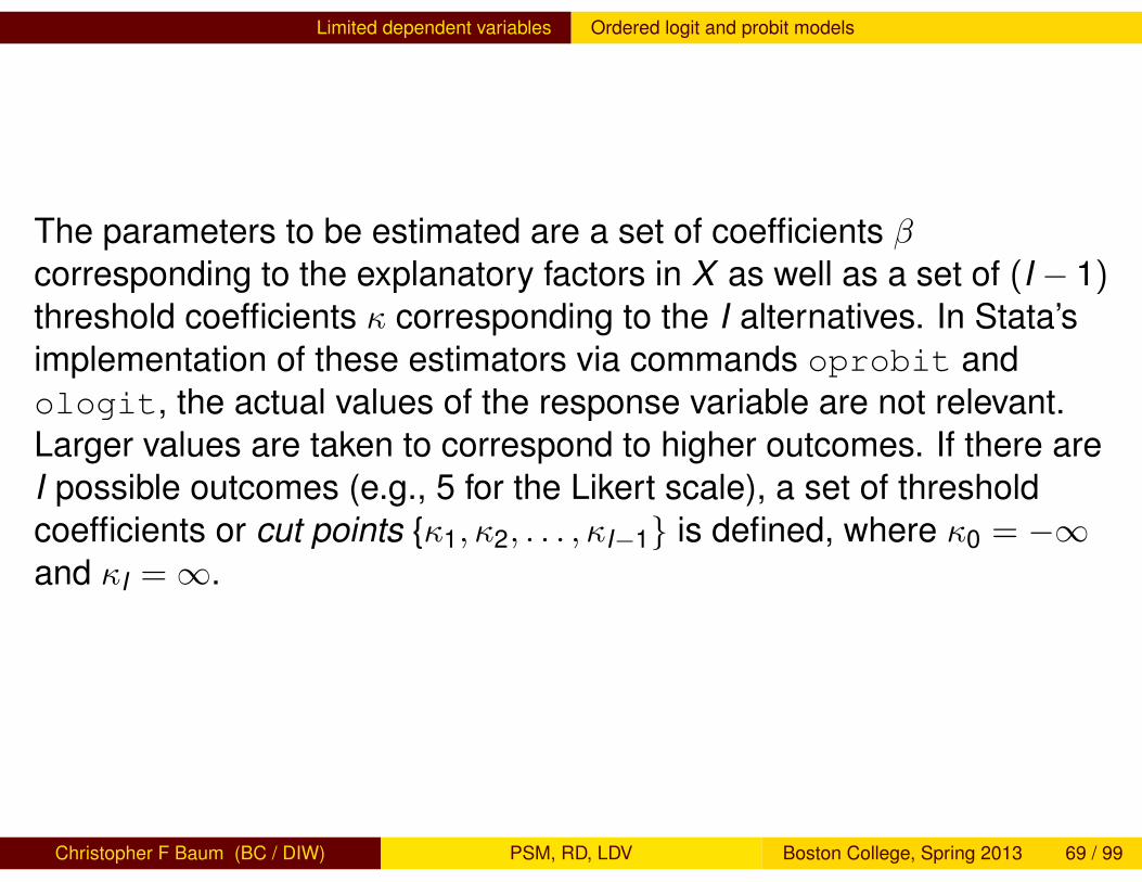
The parameters to be estimated are a set of coefficients βcorresponding to the explanatory factors in X as well as a set of (I − 1)threshold coefficients κ corresponding to the I alternatives. In Stata’simplementation of these estimators via commands oprobit andologit, the actual values of the response variable are not relevant.Larger values are taken to correspond to higher outcomes. If there areI possible outcomes (e.g., 5 for the Likert scale), a set of thresholdcoefficients or cut points {κ1, κ2, . . . , κI−1} is defined, where κ0 = −∞and κI =∞.



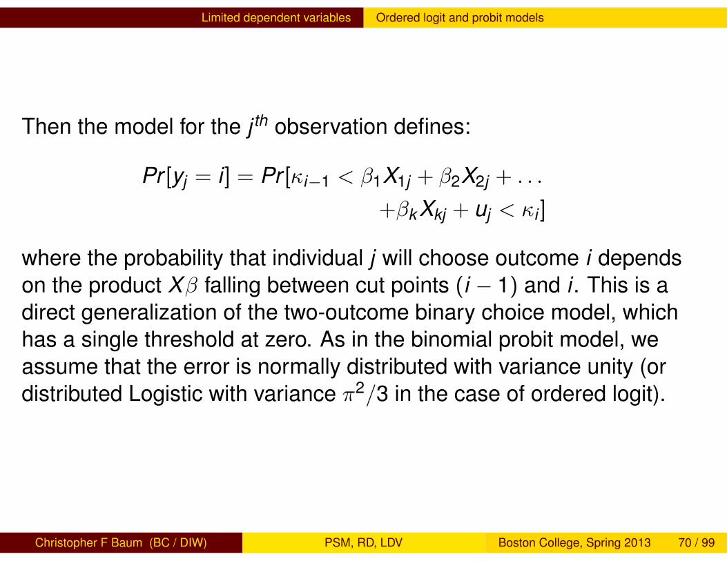
Then the model for the j th observation defines:

Pr [yj = i] = Pr [κi−1 < β1X1j + β2X2j + . . .

+βkXkj + uj < κi ]

where the probability that individual j will choose outcome i dependson the product Xβ falling between cut points (i − 1) and i . This is adirect generalization of the two-outcome binary choice model, whichhas a single threshold at zero. As in the binomial probit model, weassume that the error is normally distributed with variance unity (ordistributed Logistic with variance π2/3 in the case of ordered logit).



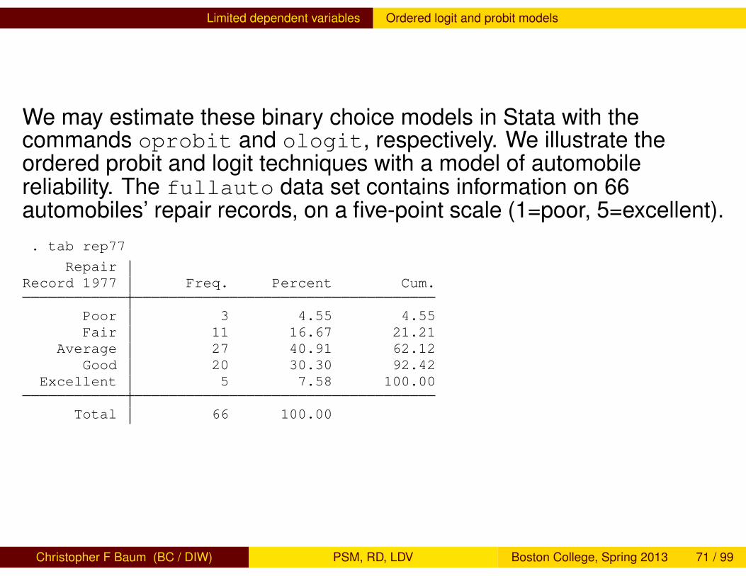
We may estimate these binary choice models in Stata with thecommands oprobit and ologit, respectively. We illustrate theordered probit and logit techniques with a model of automobilereliability. The fullauto data set contains information on 66automobiles’ repair records, on a five-point scale (1=poor, 5=excellent).. tab rep77

RepairRecord 1977 Freq. Percent Cum.

Poor 3 4.55 4.55Fair 11 16.67 21.21

Average 27 40.91 62.12Good 20 30.30 92.42

Excellent 5 7.58 100.00

Total 66 100.00



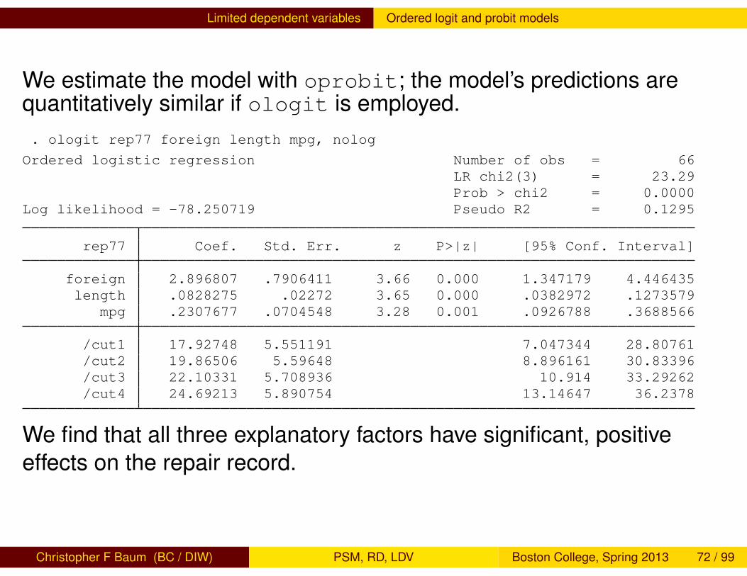
We estimate the model with oprobit; the model’s predictions arequantitatively similar if ologit is employed.. ologit rep77 foreign length mpg, nolog

Ordered logistic regression Number of obs = 66LR chi2(3) = 23.29Prob > chi2 = 0.0000


rep77 Coef. Std. Err. z P>|z| [95% Conf. Interval]

foreign 2.896807 .7906411 3.66 0.000 1.347179 4.446435length .0828275 .02272 3.65 0.000 .0382972 .1273579

mpg .2307677 .0704548 3.28 0.001 .0926788 .3688566

/cut1 17.92748 5.551191 7.047344 28.80761/cut2 19.86506 5.59648 8.896161 30.83396/cut3 22.10331 5.708936 10.914 33.29262/cut4 24.69213 5.890754 13.14647 36.2378

We find that all three explanatory factors have significant, positiveeffects on the repair record.



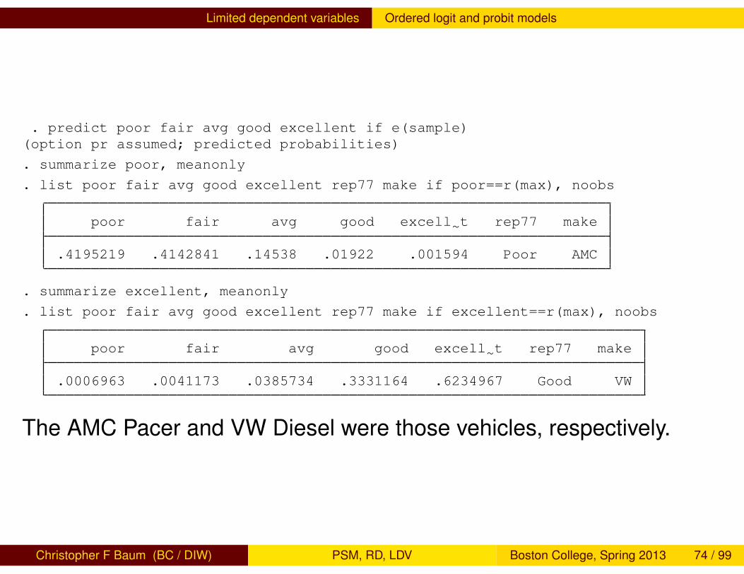
Following the ologit estimation, we employ predict to compute thepredicted probabilities of achieving each repair record. We thenexamine the automobiles who were classified as most likely to have apoor rating and an excellent rating, respectively.



. predict poor fair avg good excellent if e(sample)(option pr assumed; predicted probabilities)

. summarize poor, meanonly

. list poor fair avg good excellent rep77 make if poor==r(max), noobs

poor fair avg good excell~t rep77 make

.4195219 .4142841 .14538 .01922 .001594 Poor AMC

. summarize excellent, meanonly

. list poor fair avg good excellent rep77 make if excellent==r(max), noobs

poor fair avg good excell~t rep77 make

.0006963 .0041173 .0385734 .3331164 .6234967 Good VW

The AMC Pacer and VW Diesel were those vehicles, respectively.


Limited dependent variables Truncated regression

Truncation

We turn now to a context where the response variable is not binary nornecessarily integer, but subject to truncation. This is a bit trickier, sincea truncated or censored response variable may not be obviously so.We must fully understand the context in which the data weregenerated. Nevertheless, it is quite important that we identify situationsof truncated or censored response variables. Utilizing these variablesas the dependent variable in a regression equation withoutconsideration of these qualities will be misleading.



In the case of truncation the sample is drawn from a subset of thepopulation so that only certain values are included in the sample. Welack observations on both the response variable and explanatoryvariables. For instance, we might have a sample of individuals whohave a high school diploma, some college experience, or one or morecollege degrees. The sample has been generated by interviewingthose who completed high school.

This is a truncated sample, relative to the population, in that it excludesall individuals who have not completed high school. Thecharacteristics of those excluded individuals are not likely to be thesame as those in our sample. For instance, we might expect thataverage or median income of dropouts is lower than that of graduates.



The effect of truncating the distribution of a random variable is clear.The expected value or mean of the truncated random variable movesaway from the truncation point and the variance is reduced.Descriptive statistics on the level of education in our sample shouldmake that clear: with the minimum years of education set to 12, themean education level is higher than it would be if high school dropoutswere included, and the variance will be smaller.

In the subpopulation defined by a truncated sample, we have noinformation about the characteristics of those who were excluded. Forinstance, we do not know whether the proportion of minority highschool dropouts exceeds the proportion of minorities in the population.



A sample from this truncated population cannot be used to makeinferences about the entire population without correction for the factthat those excluded individuals are not randomly selected from thepopulation at large. While it might appear that we could use thesetruncated data to make inferences about the subpopulation, we cannoteven do that.

A regression estimated from the subpopulation will yield coefficientsthat are biased toward zero—or attenuated—as well as an estimate ofσ2

u that is biased downward.



If we are dealing with a truncated Normal distribution, wherey = Xβ + u is only observed if it exceeds τ , we may define:

αi = (τ − Xiβ)/σu

λ(αi) =φ(αi)

(1− Φ(αi))(8)

where σu is the standard error of the untruncated disturbance u, φ(·) isthe Normal density function (PDF ) and Φ(·) is the Normal CDF . Theexpression λ(αi) is termed the inverse Mills ratio, or IMR.



If a regression is estimated from the truncated sample, we find that

[yi |yi > τ,Xi ] = Xiβ + σuλ(αi) + ui (9)

These regression estimates suffer from the exclusion of the term λ(αi).This regression is misspecified, and the effect of that misspecificationwill differ across observations, with a heteroskedastic error term whosevariance depends on Xi . To deal with these problems, we include theIMR as an additional regressor. This allows us to use a truncatedsample to make consistent inferences about the subpopulation.



If we can justify making the assumption that the regression errors inthe population are Normally distributed, then we can estimate anequation for a truncated sample with the Stata command truncreg.Under the assumption of normality, inferences for the population maybe made from the truncated regression model. The estimator used inthis command assumes that the regression errors are Normal.

The truncreg option ll(#) is used to indicate that values of theresponse variable less than or equal to # are truncated. We mighthave a sample of college students with yearsEduc truncated frombelow at 12 years. Upper truncation can be handled by the ul(#)option: for instance, we may have a sample of individuals whoseincome is recorded up to $200,000. Both lower and upper truncationcan be specified by combining the options.



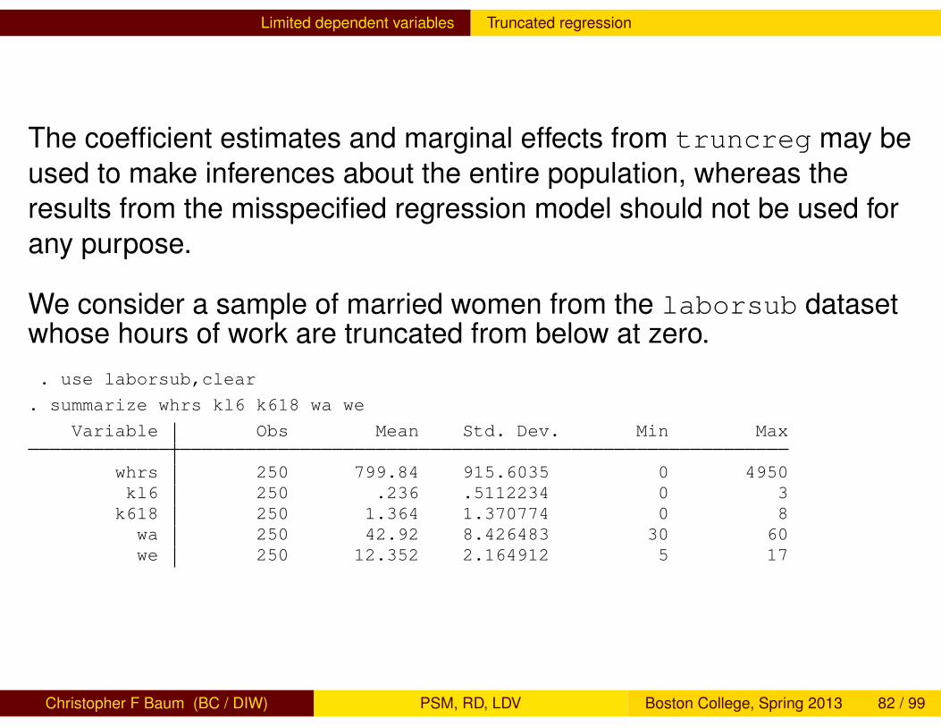
The coefficient estimates and marginal effects from truncreg may beused to make inferences about the entire population, whereas theresults from the misspecified regression model should not be used forany purpose.

We consider a sample of married women from the laborsub datasetwhose hours of work are truncated from below at zero.. use laborsub,clear

. summarize whrs kl6 k618 wa we


whrs 250 799.84 915.6035 0 4950kl6 250 .236 .5112234 0 3k618 250 1.364 1.370774 0 8wa 250 42.92 8.426483 30 60we 250 12.352 2.164912 5 17



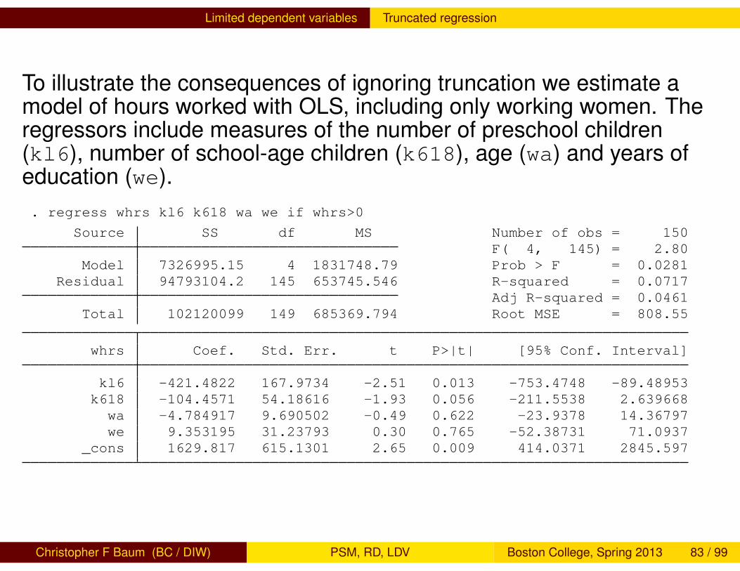
To illustrate the consequences of ignoring truncation we estimate amodel of hours worked with OLS, including only working women. Theregressors include measures of the number of preschool children(kl6), number of school-age children (k618), age (wa) and years ofeducation (we).. regress whrs kl6 k618 wa we if whrs>0

Source SS df MS Number of obs = 150F( 4, 145) = 2.80

Model 7326995.15 4 1831748.79 Prob > F = 0.0281Residual 94793104.2 145 653745.546 R-squared = 0.0717

Adj R-squared = 0.0461Total 102120099 149 685369.794 Root MSE = 808.55

whrs Coef. Std. Err. t P>|t| [95% Conf. Interval]

kl6 -421.4822 167.9734 -2.51 0.013 -753.4748 -89.48953k618 -104.4571 54.18616 -1.93 0.056 -211.5538 2.639668wa -4.784917 9.690502 -0.49 0.622 -23.9378 14.36797we 9.353195 31.23793 0.30 0.765 -52.38731 71.0937

_cons 1629.817 615.1301 2.65 0.009 414.0371 2845.597



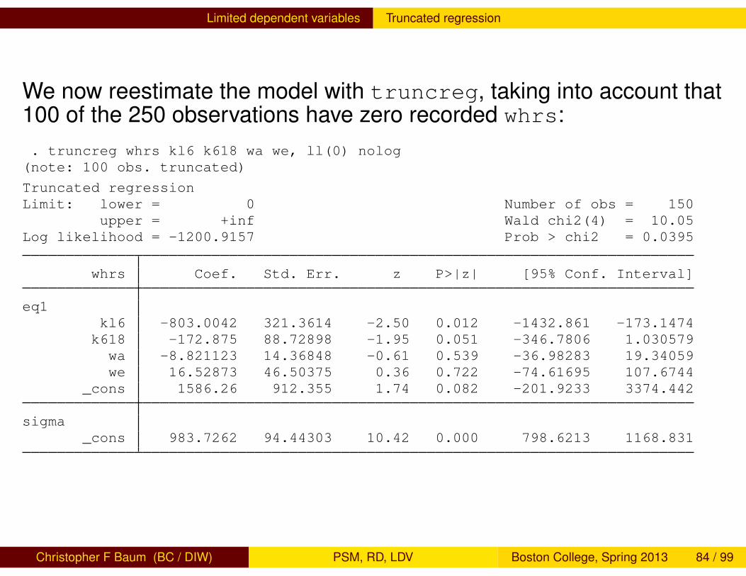
We now reestimate the model with truncreg, taking into account that100 of the 250 observations have zero recorded whrs:. truncreg whrs kl6 k618 wa we, ll(0) nolog(note: 100 obs. truncated)

Truncated regressionLimit: lower = 0 Number of obs = 150

upper = +inf Wald chi2(4) = 10.05Log likelihood = -1200.9157 Prob > chi2 = 0.0395

whrs Coef. Std. Err. z P>|z| [95% Conf. Interval]

eq1kl6 -803.0042 321.3614 -2.50 0.012 -1432.861 -173.1474k618 -172.875 88.72898 -1.95 0.051 -346.7806 1.030579wa -8.821123 14.36848 -0.61 0.539 -36.98283 19.34059we 16.52873 46.50375 0.36 0.722 -74.61695 107.6744

_cons 1586.26 912.355 1.74 0.082 -201.9233 3374.442

sigma_cons 983.7262 94.44303 10.42 0.000 798.6213 1168.831



The effect of truncation in the subsample is quite apparent. Some ofthe attenuated coefficient estimates from regress are no more thanhalf as large as their counterparts from truncreg. The parametersigma _cons, comparable to Root MSE in the OLS regression, isconsiderably larger in the truncated regression reflecting its downwardbias in a truncated sample.


Limited dependent variables Censoring

Censoring

Let us now turn to another commonly encountered issue with the data:censoring. Unlike truncation, in which the distribution from which thesample was drawn is a non-randomly selected subpopulation,censoring occurs when a response variable is set to an arbitrary valueabove or below a certain value: the censoring point. In contrast to thetruncated case, we have observations on the explanatory variables inthis sample. The problem of censoring is that we do not haveobservations on the response variable for certain individuals. Forinstance, we may have full demographic information on a set ofindividuals, but only observe the number of hours worked per week forthose who are employed.



As another example of a censored variable, consider that the numericresponse to the question “How much did you spend on a new car lastyear?” may be zero for many individuals, but that should be consideredas the expression of their choice not to buy a car.

Such a censored response variable should be considered as beinggenerated by a mixture of distributions: the binary choice to purchasea car or not, and the continuous response of how much to spendconditional on choosing to purchase. Although it would appear that thevariable caroutlay could be used as the dependent variable in aregression, it should not be employed in that manner, since it isgenerated by a censored distribution.



A solution to this problem was first proposed by Tobin (1958) as thecensored regression model; it became known as “Tobin’s probit” or thetobit model.The model can be expressed in terms of a latent variable:

y∗i = Xβ + uyi = 0 if y∗i ≤ 0 (10)yi = y∗i if y∗i > 0



As in the prior example, our variable yi contains either zeros fornon-purchasers or a dollar amount for those who chose to buy a carlast year. The model combines aspects of the binomial probit for thedistinction of yi = 0 versus yi > 0 and the regression model for[yi |yi > 0]. Of course, we could collapse all positive observations on yiand treat this as a binomial probit (or logit) estimation problem, but thatwould discard the information on the dollar amounts spent bypurchasers. Likewise, we could throw away the yi = 0 observations,but we would then be left with a truncated distribution, with the variousproblems that creates.

To take account of all of the information in yi properly, we mustestimate the model with the tobit estimation method, which employsmaximum likelihood to combine the probit and regression componentsof the log-likelihood function.



Tobit models may be defined with a threshold other than zero.Censoring from below may be specified at any point on the y scalewith the ll(#) option for left censoring. Similarly, the standard tobitformulation may employ an upper threshold (censoring from above, orright censoring) using the ul(#) option to specify the upper limit.Stata’s tobit also supports the two-limit tobit model whereobservations on y are censored from both left and right by specifyingboth the ll(#) and ul(#) options.



Even in the case of a single censoring point, predictions from the tobitmodel are quite complex, since one may want to calculate theregression-like xb with predict, but could also compute the predictedprobability that [y |X ] falls within a particular interval (which may beopen-ended on left or right).This may be specified with the pr(a,b)option, where arguments a, b specify the limits of the interval; themissing value code (.) is taken to mean infinity (of either sign).

Another predict option, e(a,b), calculates the expectationEy = E [Xβ + u] conditional on [y |X ] being in the a,b interval. Last, theystar(a,b) option computes the prediction from Equation (10): acensored prediction, where the threshold is taken into account.



The marginal effects of the tobit model are also quite complex. Theestimated coefficients are the marginal effects of a change in Xj on y∗

the unobservable latent variable:

∂E(y∗|Xj)

∂Xj= βj (11)

but that is not very useful. If instead we evaluate the effect on theobservable y , we find that:

∂E(y |Xj)

∂Xj= βj × Pr [a < y∗i < b] (12)

where a,b are defined as above for predict. For instance, forleft-censoring at zero, a = 0,b = +∞. Since that probability is at mostunity (and will be reduced by a larger proportion of censoredobservations), the marginal effect of Xj is attenuated from the reportedcoefficient toward zero.



An increase in an explanatory variable with a positive coefficient willimply that a left-censored individual is less likely to be censored. Theirpredicted probability of a nonzero value will increase. For anon-censored individual, an increase in Xj will imply that E [y |y > 0]will increase. So, for instance, a decrease in the mortgage interest ratewill allow more people to be homebuyers (since many borrowers’income will qualify them for a mortgage at lower interest rates), andallow prequalified homebuyers to purchase a more expensive home.

The marginal effect captures the combination of those effects. Sincethe newly-qualified homebuyers will be purchasing the cheapesthomes, the effect of the lower interest rate on the average price atwhich homes are sold will incorporate both effects. We expect that itwill increase the average transactions price, but due to attenuation, bya smaller amount than the regression function component of the modelwould indicate.



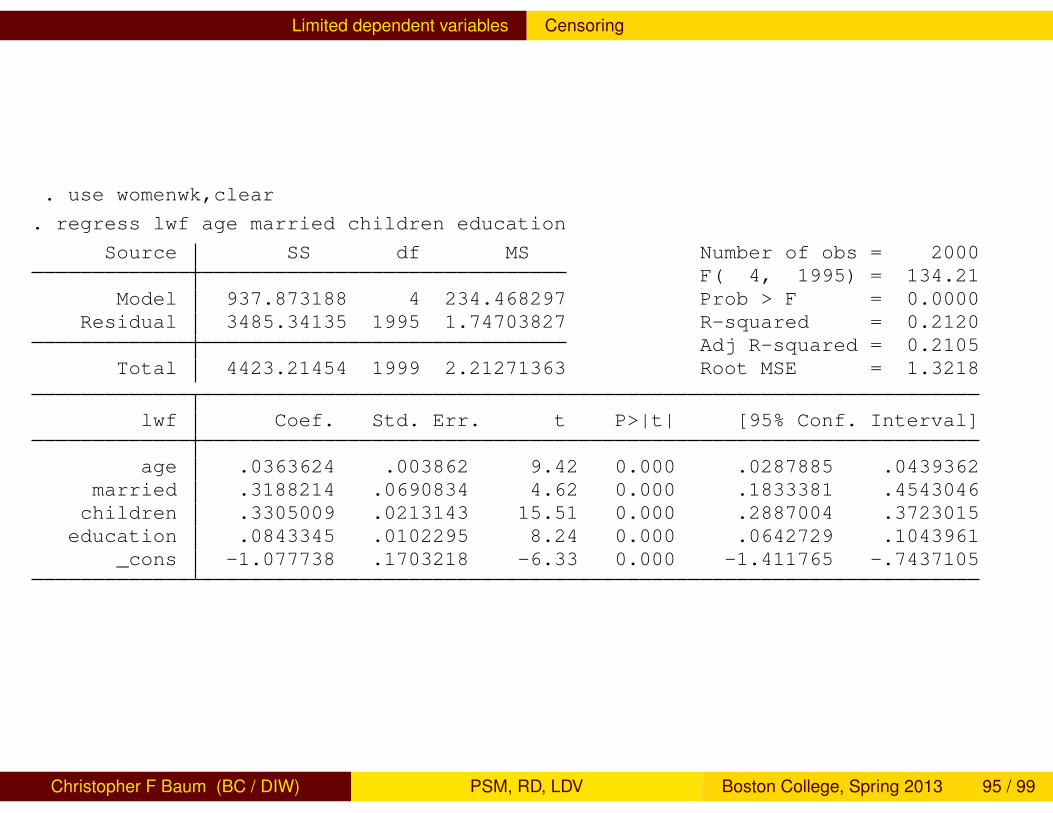
We return to the womenwk data set used to illustrate binomial probit.We generate the log of the wage (lw) for working women and set lwfequal to lw for working women and zero for non-working women. Thiscould be problematic if recorded wages below $1.00 were present inthe data, but in these data the minimum wage recorded is $5.88. Wefirst estimate the model with OLS ignoring the censored nature of theresponse variable.



. use womenwk,clear

. regress lwf age married children education

Source SS df MS Number of obs = 2000F( 4, 1995) = 134.21

Model 937.873188 4 234.468297 Prob > F = 0.0000Residual 3485.34135 1995 1.74703827 R-squared = 0.2120

Adj R-squared = 0.2105Total 4423.21454 1999 2.21271363 Root MSE = 1.3218

lwf Coef. Std. Err. t P>|t| [95% Conf. Interval]

age .0363624 .003862 9.42 0.000 .0287885 .0439362married .3188214 .0690834 4.62 0.000 .1833381 .4543046


_cons -1.077738 .1703218 -6.33 0.000 -1.411765 -.7437105



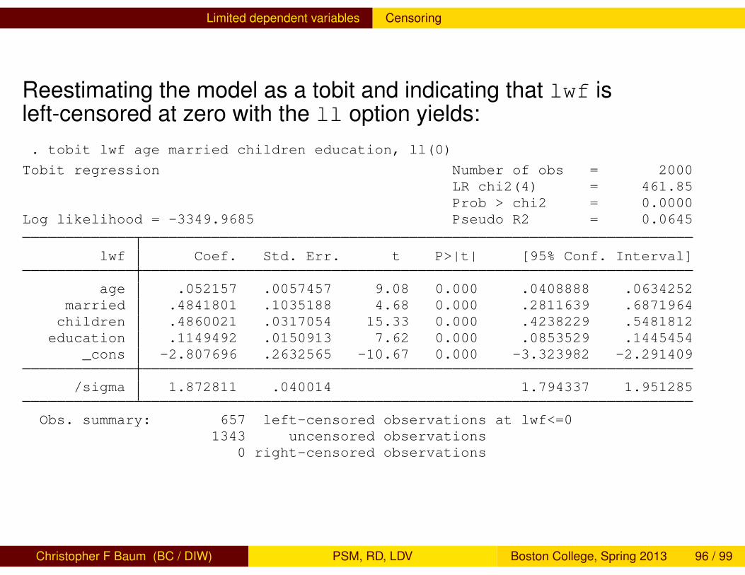
Reestimating the model as a tobit and indicating that lwf isleft-censored at zero with the ll option yields:. tobit lwf age married children education, ll(0)

Tobit regression Number of obs = 2000LR chi2(4) = 461.85Prob > chi2 = 0.0000


lwf Coef. Std. Err. t P>|t| [95% Conf. Interval]

age .052157 .0057457 9.08 0.000 .0408888 .0634252married .4841801 .1035188 4.68 0.000 .2811639 .6871964


_cons -2.807696 .2632565 -10.67 0.000 -3.323982 -2.291409

/sigma 1.872811 .040014 1.794337 1.951285

Obs. summary: 657 left-censored observations at lwf<=01343 uncensored observations

0 right-censored observations



The tobit estimates of lwf show positive, significant effects for age,marital status, the number of children and the number of years ofeducation. Each of these factors is expected to both increase theprobability that a woman will work as well as increase her wageconditional on employed status.



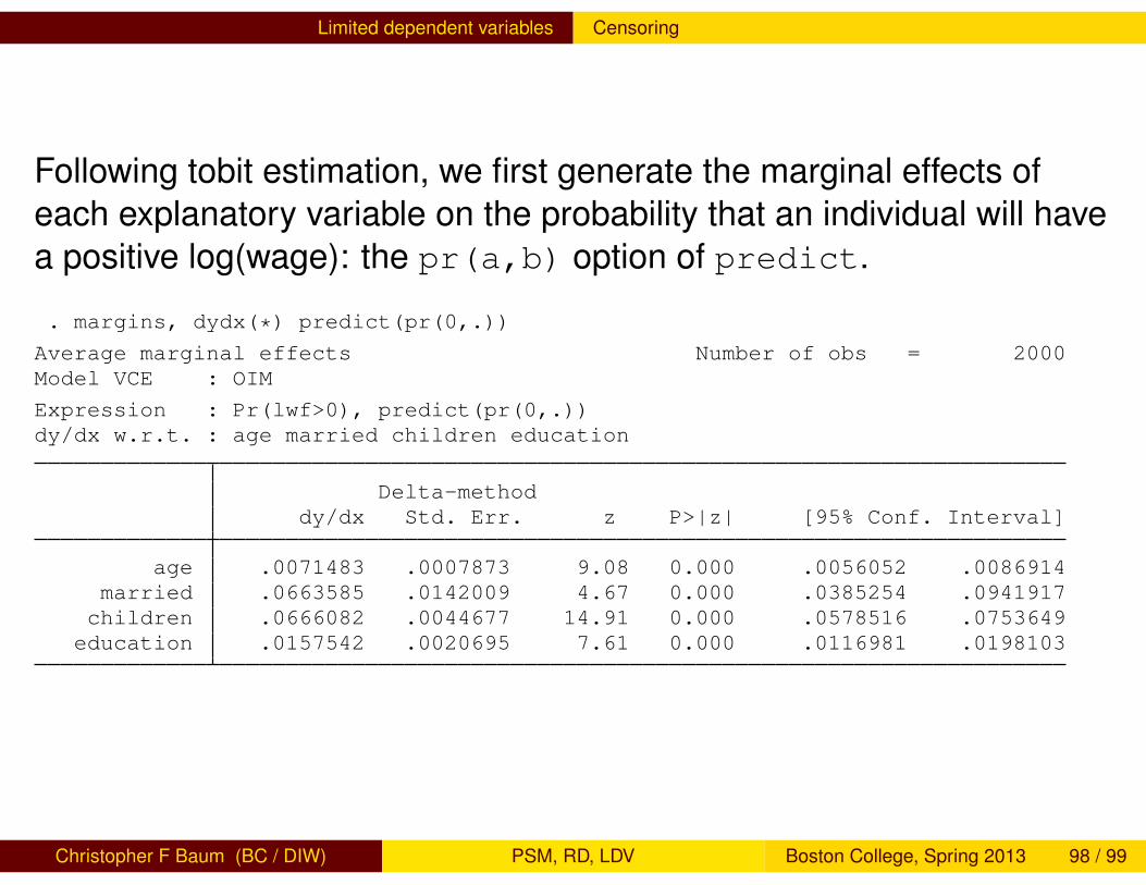
Following tobit estimation, we first generate the marginal effects ofeach explanatory variable on the probability that an individual will havea positive log(wage): the pr(a,b) option of predict.

. margins, dydx(*) predict(pr(0,.))


Expression : Pr(lwf>0), predict(pr(0,.))dy/dx w.r.t. : age married children education


age .0071483 .0007873 9.08 0.000 .0056052 .0086914married .0663585 .0142009 4.67 0.000 .0385254 .0941917




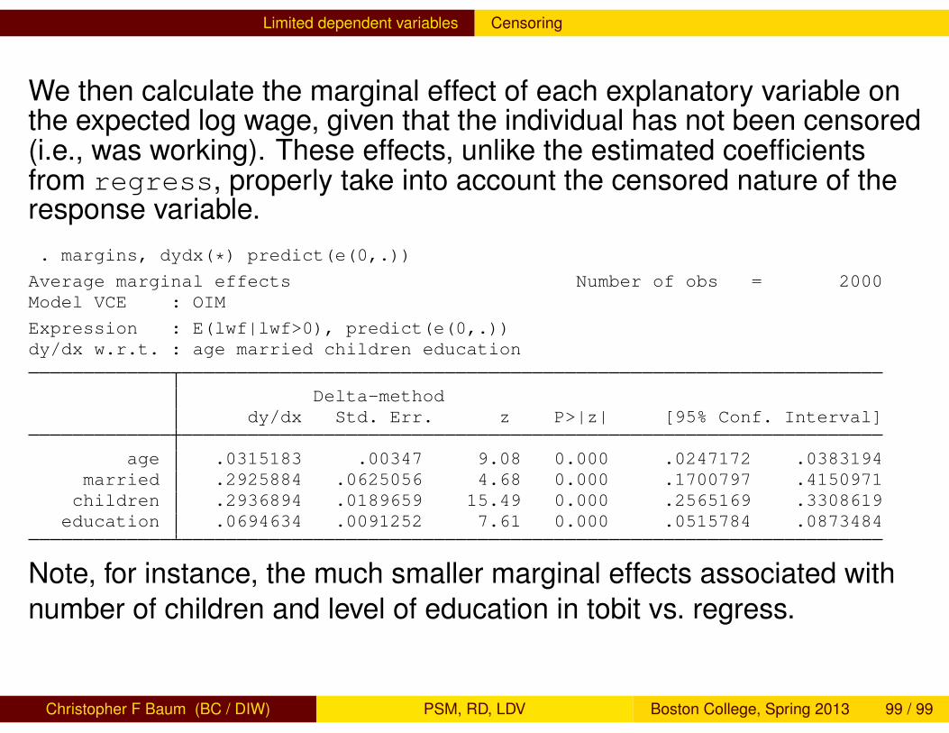
We then calculate the marginal effect of each explanatory variable onthe expected log wage, given that the individual has not been censored(i.e., was working). These effects, unlike the estimated coefficientsfrom regress, properly take into account the censored nature of theresponse variable.. margins, dydx(*) predict(e(0,.))


Expression : E(lwf|lwf>0), predict(e(0,.))dy/dx w.r.t. : age married children education


age .0315183 .00347 9.08 0.000 .0247172 .0383194married .2925884 .0625056 4.68 0.000 .1700797 .4150971


Note, for instance, the much smaller marginal effects associated withnumber of children and level of education in tobit vs. regress.
