Propagation of Electromagnetic Fields Over Flat Earth of Electromagnetic Fields Over Flat Earth ARL-TR-2352 February 2001 Joseph R. Miletta Approved for public release; distribution

Propagation of ElectromagneticFields Over Flat Earth

ARL-TR-2352 February 2001

Joseph R. Miletta

Approved for public release; distribution unlimited.

The findings in this report are not to be construed as anofficial Department of the Army position unless sodesignated by other authorized documents.

Citation of manufacturer’s or trade names does notconstitute an official endorsement or approval of the usethereof.

Destroy this report when it is no longer needed. Do notreturn it to the originator.

ARL-TR-2352 February 2001

Army Research LaboratoryAdelphi, MD 20783-1197

Propagation of ElectromagneticFields Over Flat EarthJoseph R. Miletta Sensors and Electron Devices Directorate

Approved for public release; distribution unlimited.

Abstract

This report looks at the interaction of radiated electromagnetic fields withearth ground in military or law-enforcement applications of high-powermicrowave (HPM) systems. For such systems to be effective, the microwavepower density on target must be maximized. The destructive and construc-tive scattering of the fields as they propagate to the target will determinethe power density at the target for a given source. The question of fieldpolarization arises in designing an antenna for an HPM system. Shouldthe transmitting antenna produce vertically, horizontally, or circularly po-larized fields? Which polarization maximizes the power density on target?This report provides a partial answer to these questions. The problems ofcalculating the reflection of uniform plane wave fields from a homogeneousboundary and calculating the fields from a finite source local to a perfectlyconducting boundary are relatively straightforward. However, when thesource is local to a general homogeneous plane boundary, the solution can-not be expressed in closed form. An approximation usually of the formof an asymptotic expansion results. Calculations of the fields are providedfor various source and target locations for the frequencies of interest. Theconclusion is drawn that the resultant vertical field from an appropriatelyoriented source antenna located near and above the ground can be signif-icantly larger than a horizontally polarized field radiated from the samelocation at a 1.3 GHz frequency at observer locations near and above theground.

ii

Contents

1 Introduction 1

2 Problem Formulation 2

2.1 Vertical Dipole Over Earth . . . . . . . . . . . . . . . . . . . . 3

2.2 Horizontal Dipole Over Earth . . . . . . . . . . . . . . . . . . 4

2.3 Comparisons . . . . . . . . . . . . . . . . . . . . . . . . . . . . 5

2.3.1 Comparison of Field Components Near the Earth . . 6

3 Conclusion 14

References 15

Appendix. MATLAB m-Files 17

Distribution 27

Report Documentation Page 29

Figures

1 Geometry for vertical and horizontal dipole formulations . . . . 2

2 Comparison of main electric field components from a vertical(Ez) and from a horizontal (Eφ) broadside ideal dipole over aperfectly conducting ground . . . . . . . . . . . . . . . . . . . . . 7

3 Reflection coefficients for vertically and horizontally polarizedplane waves of 1.3-GHz frequency incident on a flat ground forfive earth-parameter cases listed in table 1 . . . . . . . . . . . . . 8

4 Fresnel reflection coefficient for a vertically polarized plane wavefield compared to “reflection coefficient” as calculated by com-plete formulation for a vertical dipole over homogeneous earthas observed at 1-m height 1000 m down range at a frequency of1.3 GHz . . . . . . . . . . . . . . . . . . . . . . . . . . . . . . . . . 9

5 Fresnel reflection coefficient for a horizontally polarized planewave field compared to “reflection coefficient” as calculated bycomplete formulation for a horizontal dipole over homogeneousearth as observed at 1-m height, broadside 1000 m down rangeat a frequency of 1.3 GHz . . . . . . . . . . . . . . . . . . . . . . 10

iii

6 Comparison of principal fields from an ideal dipole orientedperpendicular and horizontal to a homogeneous flat earth . . . 11

7 Comparison of principal fields from an ideal dipole orientedperpendicular and horizontal to a homogeneous flat earth . . . 12

8 Effect of ground reflection on primary field components nearground for typical earth parameters . . . . . . . . . . . . . . . . 13

Tables

1 Earth parameters . . . . . . . . . . . . . . . . . . . . . . . . . . . 6

iv

1. Introduction

Effective military or law-enforcement applications of high-power mi-crowave (HPM) systems in which the HPM system and the target systemare on or near the ground or water require that the microwave power den-sity on target be maximized. The power density at the target for a givensource will depend on the destructive and constructive scattering of thefields as they propagate to the target. Antenna design for an HPM sys-tem includes addressing the following questions about field polarization:Should the fields the transmitting antenna produces be vertically, hori-zontally, or circularly polarized? Which polarization maximizes the powerdensity on target? (The question of which polarization best couples to thetarget is beyond the scope of this report.) While this report does not com-pletely answer these questions, it addresses the interaction of the radiatedelectromagnetic fields with earth ground. It is assumed that the transmit-ting antenna and the target (or receiver) are located above, but near thesurface of a flat idealized earth (constant permittivity, ε, and conductivity,σ) ground. First an ideal vertical dipole (oriented along the z-axis perpen-dicular to the ground plane) is addressed. The horizontal dipole (parallelto the ground plane) follows.

1

2. Problem Formulation

The problems of calculating the reflection of uniform plane wave fieldsfrom a homogeneous boundary and calculating the fields from a finitesource local to a perfectly conducting boundary are relatively straightfor-ward. However, when the source is local to a general homogeneous planeboundary, it is found that the solution cannot be expressed in closed form.An approximation usually of the form of an asymptotic expansion results.The problem of an ideal dipole over a homogeneous half-space has been thetopic of a number of studies starting at the turn of the last century with thesolution provided by Sommerfeld (1949) and leading to the more contem-porary work of Banos (1966) and King et al (1994, 1992). References suchas Maclean and Wu (1993) address in detail the many approaches to solv-ing the problem. Considerable controversy has surrounded these studies.We will not attempt to derive the solution or otherwise discuss the solu-tion of the problem in this report. We will rely on the work of King et alfor a complete and concise formulation of the problem. Figure 1 depicts theproblem geometry. The King expressions have been encoded and solved inMATLAB (1984–1999). Comparisons of the field structures are providedfor various source and target locations for frequencies of interest.

The expressions that follow are constrained by the magnitude of the wavenumbers (k = ω(µε)1/2, ω = 2π× frequency) in each region:

|k1| ≥ 3 |k2| , (1)

where, after King, the subscript 2 denotes the upper half-space (air) and thesubscript 1 denotes the lower half-space (earth). Also, µ is the permeabilityin henries per meter, ε is the permittivity in farads per meter, and σ is theconductivity in siemens per meter. The subscripts 0 and r represent freespace and relative to free space, respectively.

Figure 1. Geometry forvertical and horizontaldipole formulations.

z

z′

0

r0

r1

r2Region 2µ0, ε0, σ = 0

Region 1µ0, ε2 = εr ε0,σ ≠ 0

y

x

Looking down

θd

θd

φ

ρ

Ψ

2

2.1 Vertical Dipole Over Earth

The electromagnetic fields from a dipole with dipole moment I orientedperpendicular to and at a height z = d above the ground plane have threecomponents in cylindrical coordinates. The magnetic field is symmetricabout the z-axis, perpendicular to the direction of propagation. For thatreason the fields will be termed transverse magnetic (TM) fields. (We willfind that the horizontal dipole has TM and transverse electric (TE) com-ponents.) The formulation as provided in King et al (1994) is, referring tofigure 1,

Hφ(ρ, z) = − I

2π

eik2r1

2

(ρr1

) (ik2r1

− 1r21

)+ eik2r2

2

(ρr2

) (ik2r2

− 1r22

)−eik2r2

(k32

k1

) (π

k2r2

) 12 e−iPF (P )

, (2)

Eρ(ρ, z) = −ωµ0I

2πk2

eik2r1

2

(ρr1

) (z−dr1

) (ik2r1

− 3r21− 3i

k2r31

)+ eik2r2

2

(ρr2

) (z+dr2

) (ik2r2

− 3r22− 3i

k2r32

)−k2

k1eik2r2

[(ρr2

) (ik2r2

− 1r22

)−

(k32

k1

) (π

k2r2

) 12 e−iPF (P )

]

, and (3)

Ez(ρ, z) =ωµ0I

2πk2

eik2r1

2

[(ik2r1

− 1r21− i

k2r31

)−

(z−dr1

)2 (ik2r1

− 3r21− 3i

k2r31

)]

+ eik2r2

2

[(ik2r2

− 1r22− i

k2r32

)−

(z+dr2

)2 (ik2r2

− 3r22− 3i

k2r32

)]

−eik2r2k32

k1

(ρr2

) (π

k2r2

) 12 e−iPF (P )

, (4)

where

r1 =[ρ2 + (z − d)2

] 12 ,

r2 =[ρ2 + (z + d)2

] 12 , (5)

P =k3

2r22k2

1

(k2r2 + k1 (z + d)

k2ρ

)2

, (6)

F (P ) =∫ ∞

P

eit

(2πt)12

dt =12

(1 + i) − C2 (P ) − iS2 (P ) , (7)

and C2(P ), S2(P ) are the Fresnel integrals as defined in Abramowitz andStegun (1970). Since

C2 (P ) + iS2 (P ) =12

(1 + i) −√i

2eiPw

(√iP

), (8)

we have

F (P ) =

√i

2eiPw

(√iP

), (9)

where w(z), called the plasma dispersion function with complex argument,is a form of the error function defined in Abramowitz and Stegun (1970). A

3

convenient MATLAB m-file is available for solving the function with com-plex argument (Chase) and is provided in the appendix. Note that

√i can

be written as (i+1)2 and that F (P ) always appears with e−iP , thus cancel-

ing the exponential term in equation (9). This is reflected in the MATLAB

m-files that calculate the fields (provided in the appendix).

The equations have been written such that the direct and reflected compo-nents appear first. The last term is referred to as the surface or lateral wave.Often it is called the Norton surface wave from the engineering models hedeveloped in the mid-1930s. The equations reduce to the fields above a per-fectly conducting ground when k1 → ∞; the surface or lateral wave termthen goes to zero.

2.2 Horizontal Dipole Over Earth

The electromagnetic fields produced by an ideal dipole oriented at a heightz = d above and parallel to the ground plane consist in general of both TMand TE components. The formulation as provided in King et al (1992) forthe TM wave components in cylindrical coordinates, referring to figure 1and the above definitions, is

Hφ(ρ, φ, z) =I

4πcosφ

eik2r1

(z−dr1

) (ik2r1

− 1r21

)− eik2r2

(z+dr2

) (ik2r2

− 1r22

)

+2k2k1eik2r2

ik2r2

− 1r22− i

k2r32

−(

k32

k1

) (r2ρ

) (π

k2r2

) 12 e−iPF (P )

, (10)

Eρ(ρ, φ, z) =ωµ0I

4πk2cosφ

eik2r1

[2r21

+ 2ik2r3

1+

(z−dr1

)2 (ik2r1

− 3r21− 3i

k2r31

)]

−eik2r2

2r22

+ 2ik2r3

2+

(z+dr2

)2 (ik2r2

− 3r22− 3i

k2r32

)−2k2

k1

(z+dr2

) (ik2r2

− 1r22

)

+2k22

k21

ik2r2

− 1r22− i

k2r32

−(

k32

k1

) (r2ρ

) (π

k2r2

) 12 e−iPF (P )

, and (11)

Ez(ρ, φ, z) =ωµ0I

4πk2cosφ

−eik2r1

(ρr1

) (z−dr1

) (ik2r1

− 3r21− 3i

k2r31

)+eik2r2

(ρr2

) (z+dr2

) (ik2r2

− 3r22− 3i

k2r32

)−2k2

k1eik2r2

[(ρr2

) (ik2r2

− 1r22

)− k3

2k1

(π

k2r2

) 12 e−iPF (P )

]

. (12)

The TM fields are zero broadside to the dipole orientation, φ = π2 . The TE

components are

4

Hρ(ρ, φ, z) =I

4πsinφ

eik2r1

(z−dr1

) (ik2r1

− 1r21

)− eik2r2

(z+dr2

) (ik2r2

− 1r22

)

+2k2k1eik2r2

2

r22

+ 2ik2r3

2+

(ik2

2k1ρ

) (r22

ρ2

) (π

k2r2

) 12 e−iPF (P )

+(

z+dr2

)2 (ik2r2

− 3r22− 3i

k2r32

)

, (13)

Hz(ρ, φ, z) =I

4πsinφ

eik2r1

(ρr1

) (ik2r1

− 1r21

)− eik2r2

(ρr2

) (ik2r2

− 1r22

)

+2(

ρr2

)eik2r2

(k2k1

) (z+dr2

) (ik2r2

− 3r22− 3i

k2r32

)

−(

k2k1

)2

1r22

+ 3ik2r3

2− 3

k22r4

2+(

z+dr2

)2 (ik2r2

− 6r22− 15i

k2r32

)

, and (14)

Eφ(ρ, φ, z) = −ωµ0I

4πk2sinφ

eik2r1

(ik2r1

+ 1r21− i

k2r31

)− eik2r2

(ik2r2

− 1r22− i

k2r32

)

−eik2r2

−2k2k1

(z+dr2

) (ik2r2

− 1r22

)

+2k22

k21

2r22

+ 2ik2r3

2

+(

z+dr2

)2 (ik2r2

− 3r22− 3i

k2r32

)

+(

2ik42

k31ρ

) (r2ρ

)2 (π

k2r2

) 12 e−iPF (P )

. (15)

These are the predominant fields broadside to the dipole orientation. HereEφ is often termed the horizontal electric field. Again, the equations reduceto the fields above a perfectly conducting ground when k1 → ∞; the surfaceor lateral wave term goes to zero.

2.3 Comparisons

The peak power radiated by a unit dipole is given in Collin and Zucker(1969):

P =k2

2ζ012π

, (16)

where ζ0 is the free-space impedance(√

µ0

ε0

). The fields and power density

comparisons that follow are normalized to one watt radiated peak power.To obtain the unnormalized quantities, simply multiply the power resultsby P and the field results by P

12 . The outward component of the complex

Poynting vector over a closed surface is

1/2

∮S

E ×H ∗ · dS = −Pcomplex , (17)

where the negative sign indicates power flow away from the surface. Ourinterest is in the real part of the power density at the observer (or target)location. In our cylindrical coordinate system for the TM components, thisbecomes

1/2 Re (E ×H∗) = 1/2 Re(ρ0EzHφ

∗ + z0EρHφ∗), (18)

5

where ρ0

and z0 are the unit vectors in cylindrical coordinates. Near theground, the power flow is predominantly radial with a small z component.And, for the TE components, we have

1/2 Re (E ×H∗) = 1/2 Re(ρ0EφHz

∗ − z0EφHρ∗). (19)

For the vertical dipole, the power density at the observer (on target) will be

Pv = 1/2 (Re (EφHz∗) + Re (EφHρ

∗)) . (20)

The horizontal dipole in general will produce a target power density of

Ph = 1/2 ({Re (EφHz∗) − Re (EzHφ

∗)} + {Re (EρHφ∗) − Re (EφHρ

∗)}) . (21)

For broadside calculations this becomes

Ph = 1/2 (Re (EφHz∗) + Re (EφHρ

∗)) . (22)

The calculations that follow are limited to a frequency of 1.3 GHz (wave-length, λ0, is 0.23 m) and dipole heights of 1 to 3 m. Observer (target)heights range from 0 to 5 m. The frequency of 1.3 GHz is chosen, since mostof the HPM source and antenna design work at ARL is centered around thatfrequency. The height ranges are chosen to be consistent with ground vehi-cle source and target applications. Five classes of ground parameters thatare representative of distinctly different terrain will be addressed. Thesefive classes are those discussed in King et al (1994) and are given in table 1.

2.3.1 Comparison of Field Components Near the Earth

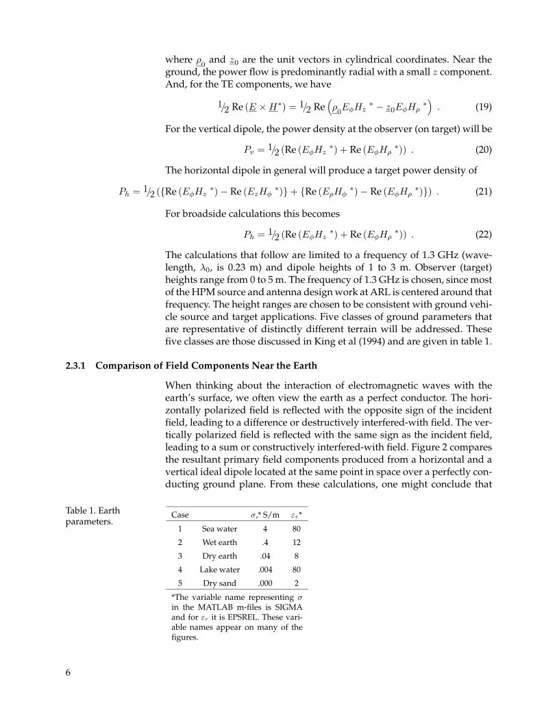
When thinking about the interaction of electromagnetic waves with theearth’s surface, we often view the earth as a perfect conductor. The hori-zontally polarized field is reflected with the opposite sign of the incidentfield, leading to a difference or destructively interfered-with field. The ver-tically polarized field is reflected with the same sign as the incident field,leading to a sum or constructively interfered-with field. Figure 2 comparesthe resultant primary field components produced from a horizontal and avertical ideal dipole located at the same point in space over a perfectly con-ducting ground plane. From these calculations, one might conclude that

Table 1. Earthparameters.

Case σ,* S/m εr*

1 Sea water 4 80

2 Wet earth .4 12

3 Dry earth .04 8

4 Lake water .004 80

5 Dry sand .000 2

*The variable name representing σin the MATLAB m-files is SIGMAand for εr it is EPSREL. These vari-able names appear on many of thefigures.

6

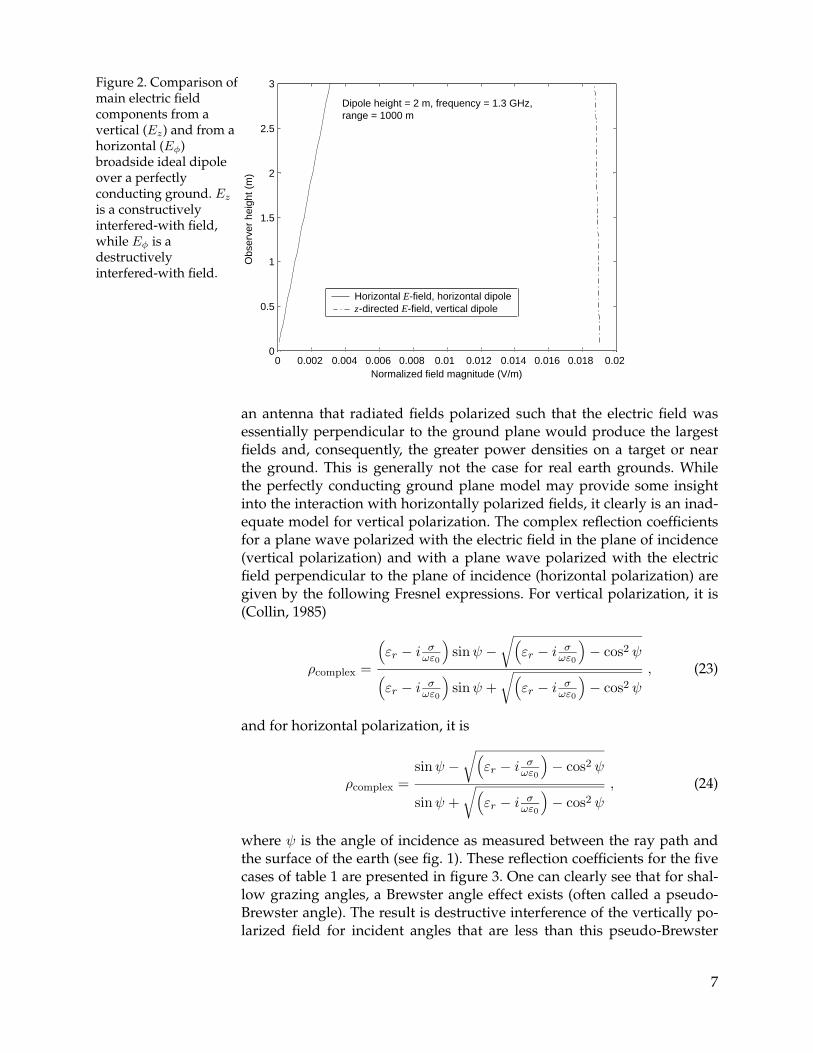
Figure 2. Comparison ofmain electric fieldcomponents from avertical (Ez) and from ahorizontal (Eφ)broadside ideal dipoleover a perfectlyconducting ground. Ez

is a constructivelyinterfered-with field,while Eφ is adestructivelyinterfered-with field.

0 0.002 0.004 0.006 0.008 0.01 0.012 0.014 0.016 0.018 0.020

0.5

1

1.5

2

2.5

3

Dipole height = 2 m, frequency = 1.3 GHz,range = 1000 m

Normalized field magnitude (V/m)

Horizontal E-field, horizontal dipolez-directed E-field, vertical dipole

Obs

erve

r he

ight

(m

)

an antenna that radiated fields polarized such that the electric field wasessentially perpendicular to the ground plane would produce the largestfields and, consequently, the greater power densities on a target or nearthe ground. This is generally not the case for real earth grounds. Whilethe perfectly conducting ground plane model may provide some insightinto the interaction with horizontally polarized fields, it clearly is an inad-equate model for vertical polarization. The complex reflection coefficientsfor a plane wave polarized with the electric field in the plane of incidence(vertical polarization) and with a plane wave polarized with the electricfield perpendicular to the plane of incidence (horizontal polarization) aregiven by the following Fresnel expressions. For vertical polarization, it is(Collin, 1985)

ρcomplex =

(εr − i σ

ωε0

)sinψ −

√(εr − i σ

ωε0

)− cos2 ψ

(εr − i σ

ωε0

)sinψ +

√(εr − i σ

ωε0

)− cos2 ψ

, (23)

and for horizontal polarization, it is

ρcomplex =sinψ −

√(εr − i σ

ωε0

)− cos2 ψ

sinψ +√(

εr − i σωε0

)− cos2 ψ

, (24)

where ψ is the angle of incidence as measured between the ray path andthe surface of the earth (see fig. 1). These reflection coefficients for the fivecases of table 1 are presented in figure 3. One can clearly see that for shal-low grazing angles, a Brewster angle effect exists (often called a pseudo-Brewster angle). The result is destructive interference of the vertically po-larized field for incident angles that are less than this pseudo-Brewster

7

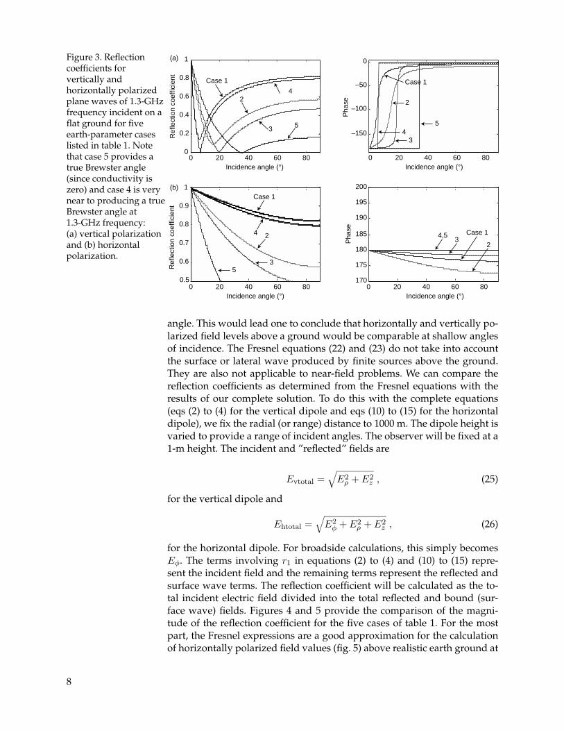
Figure 3. Reflectioncoefficients forvertically andhorizontally polarizedplane waves of 1.3-GHzfrequency incident on aflat ground for fiveearth-parameter caseslisted in table 1. Notethat case 5 provides atrue Brewster angle(since conductivity iszero) and case 4 is verynear to producing a trueBrewster angle at1.3-GHz frequency:(a) vertical polarizationand (b) horizontalpolarization.

0 20 40 60 800

0.2

0.4

0.6

0.8

1

Incidence angle (°)

–150

–100

–50

0

170

175

180

185

190

195

200

Case 1

2

5 3

4

4,5

0 20 40 60 80Incidence angle (°)



0.5

0.6

0.7

0.8

0.9

1

Ref

lect

ion

coef

ficie

nt

Pha

seP

hase

Ref

lect

ion

coef

ficie

nt

(a)

(b)

Case 1

5

2

43

53

24

Case 1

3Case 1

2

angle. This would lead one to conclude that horizontally and vertically po-larized field levels above a ground would be comparable at shallow anglesof incidence. The Fresnel equations (22) and (23) do not take into accountthe surface or lateral wave produced by finite sources above the ground.They are also not applicable to near-field problems. We can compare thereflection coefficients as determined from the Fresnel equations with theresults of our complete solution. To do this with the complete equations(eqs (2) to (4) for the vertical dipole and eqs (10) to (15) for the horizontaldipole), we fix the radial (or range) distance to 1000 m. The dipole height isvaried to provide a range of incident angles. The observer will be fixed at a1-m height. The incident and ”reflected” fields are

Evtotal =√E2

ρ + E2z , (25)

for the vertical dipole and

Ehtotal =√E2

φ + E2ρ + E2

z , (26)

for the horizontal dipole. For broadside calculations, this simply becomesEφ. The terms involving r1 in equations (2) to (4) and (10) to (15) repre-sent the incident field and the remaining terms represent the reflected andsurface wave terms. The reflection coefficient will be calculated as the to-tal incident electric field divided into the total reflected and bound (sur-face wave) fields. Figures 4 and 5 provide the comparison of the magni-tude of the reflection coefficient for the five cases of table 1. For the mostpart, the Fresnel expressions are a good approximation for the calculationof horizontally polarized field values (fig. 5) above realistic earth ground at

8

Figure 4. Fresnelreflection coefficient fora vertically polarizedplane wave fieldcompared to “reflectioncoefficient” ascalculated by completeformulation for avertical dipole overhomogeneous earth asobserved at 1-m height1000 m down range at afrequency of 1.3 GHz:(a) sea water, (b) wetearth, (c) dry earth,(d) lake water, and(e) dry sand.

0 10 20 30 40 50 60 70 80 900

0.1

0.2

0.3

0.4

0.5

0.6

0.7

0.8

0.9

1

Incidence angle (°)R

efle

ctio

n co

effic

ient

0 10 20 30 40 50 60 70 80 900

0.1

0.2

0.3

0.4

0.5

0.6

0.7

0.8

0.9

1


Ref

lect

ion

coef

ficie

nt

0 10 20 30 40 50 60 70 80 900

0.1

0.2

0.3

0.4

0.5

0.6

0.7

0.8

0.9

1


Ref

lect

ion

coef

ficie

nt

0 10 20 30 40 50 60 70 80 900

0.1

0.2

0.3

0.4

0.5

0.6

0.7

0.8

0.9

1


Ref

lect

ion

coef

ficie

nt

0 10 20 30 40 50 60 70 80 900

0.1

0.2

0.3

0.4

0.5

0.6

0.7

0.8

0.9

1


Ref

lect

ion

coef

ficie

nt

(a)

(c)

(e)

(d)

(b)

SIGMA = 4 S/m, EPSREL= 80

Fresnel Eq.Complete Eq.

SIGMA = 0.4 S/m, EPSREL= 12

SIGMA = 0.04 S/m, EPSREL= 8 SIGMA = 0.004 S/m, EPSREL= 80

SIGMA = 0 S/m, EPSREL= 2





1.3 GHz. The horizontally polarized fields diverge from the Fresnel expres-sions for low conductivities and relative dielectric constants. The resultingtotal fields in such cases predicted by the Fresnel expressions will be largerthan the complete solution prediction. The results for vertical polarization(fig. 4) show significant divergence for shallow incident angles. In this casethe resulting total fields predicted by the complete solution can be signifi-cantly higher than that predicted from employing the Fresnel expressions.

9

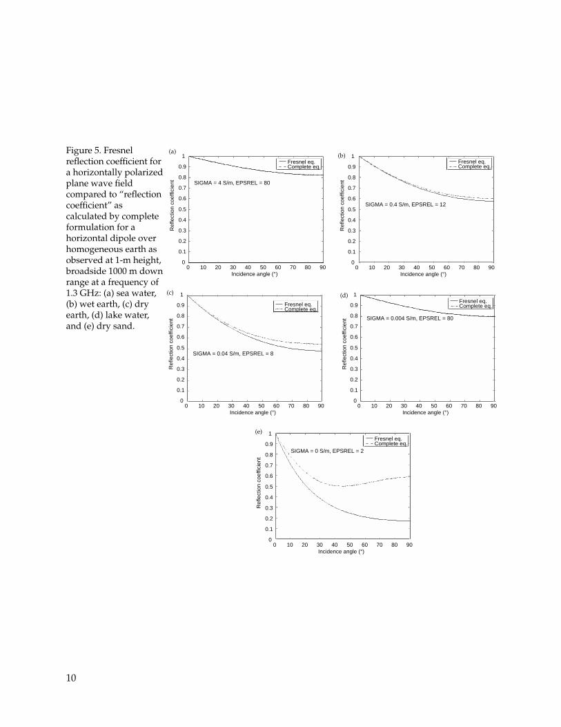
Figure 5. Fresnelreflection coefficient fora horizontally polarizedplane wave fieldcompared to “reflectioncoefficient” ascalculated by completeformulation for ahorizontal dipole overhomogeneous earth asobserved at 1-m height,broadside 1000 m downrange at a frequency of1.3 GHz: (a) sea water,(b) wet earth, (c) dryearth, (d) lake water,and (e) dry sand.

0 10 20 30 40 50 60 70 80 900

0.1

0.2

0.3

0.4

0.5

0.6

0.7

0.8

0.9

1


SIGMA = 4 S/m, EPSREL = 80

Fresnel eq. Complete eq.

Ref

lect

ion

coef

ficie

nt

0 10 20 30 40 50 60 70 80 900

0.1

0.2

0.3

0.4

0.5

0.6

0.7

0.8

0.9

1


SIGMA = 0.4 S/m, EPSREL = 12

Ref

lect

ion

coef

ficie

nt

0 10 20 30 40 50 60 70 80 900

0.1

0.2

0.3

0.4

0.5

0.6

0.7

0.8

0.9

1



Ref

lect

ion

coef

ficie

nt

0 10 20 30 40 50 60 70 80 900

0.1

0.2

0.3

0.4

0.5

0.6

0.7

0.8

0.9

1



Ref

lect

ion

coef

ficie

nt

0 10 20 30 40 50 60 70 80 900

0.1

0.2

0.3

0.4

0.5

0.6

0.7

0.8

0.9

1


SIGMA = 0 S/m, EPSREL = 2

Ref

lect

ion

coef

ficie

nt

(a)

(c)

(e)

(d)

(b)





10

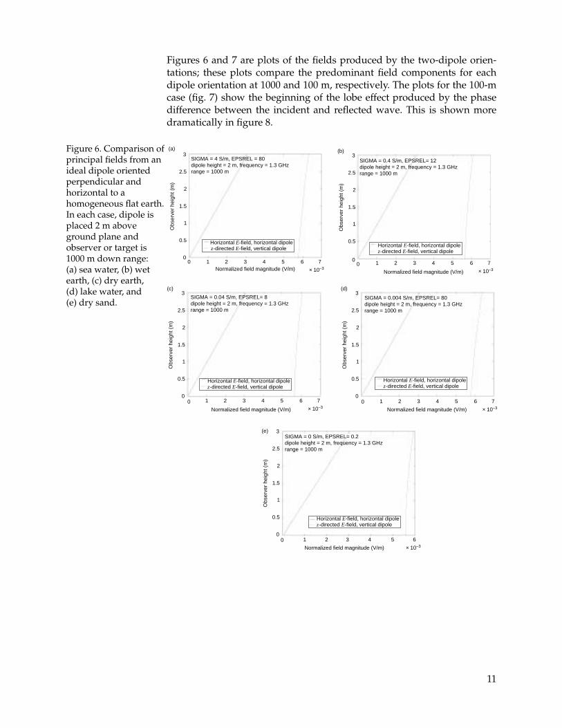
Figures 6 and 7 are plots of the fields produced by the two-dipole orien-tations; these plots compare the predominant field components for eachdipole orientation at 1000 and 100 m, respectively. The plots for the 100-mcase (fig. 7) show the beginning of the lobe effect produced by the phasedifference between the incident and reflected wave. This is shown moredramatically in figure 8.

Figure 6. Comparison ofprincipal fields from anideal dipole orientedperpendicular andhorizontal to ahomogeneous flat earth.In each case, dipole isplaced 2 m aboveground plane andobserver or target is1000 m down range:(a) sea water, (b) wetearth, (c) dry earth,(d) lake water, and(e) dry sand.

0 1 2 3 4 5 6 7

× 10–3

0

0.5

1

1.5

2

2.5

3


Obs

erve

r he

ight

(m

)

(a)

00

0.5

1

1.5

2

2.5

3


Obs

erve

r he

ight

(m

)

(d)

00

0.5

1

1.5

2

2.5

3


Obs

erve

r he

ight

(m

)

(e)

00

0.5

1

1.5

2

2.5

3


Obs

erve

r he

ight

(m

)

(c)

00

0.5

1

1.5

2

2.5

3


Obs

erve

r he

ight

(m

)

(b)

SIGMA = 4 S/m, EPSREL = 80dipole height = 2 m, frequency = 1.3 GHzrange = 1000 m


SIGMA = 0.4 S/m, EPSREL= 12dipole height = 2 m, frequency = 1.3 GHzrange = 1000 m



SIGMA = 0 S/m, EPSREL= 0.2dipole height = 2 m, frequency = 1.3 GHzrange = 1000 m

1 2 3 4 5 6 7

× 10–3

1 2 3 4 5 6 7

× 10–31 2 3 4 5 6 7

× 10–3

1 2 3 4 5 6

× 10–3





11

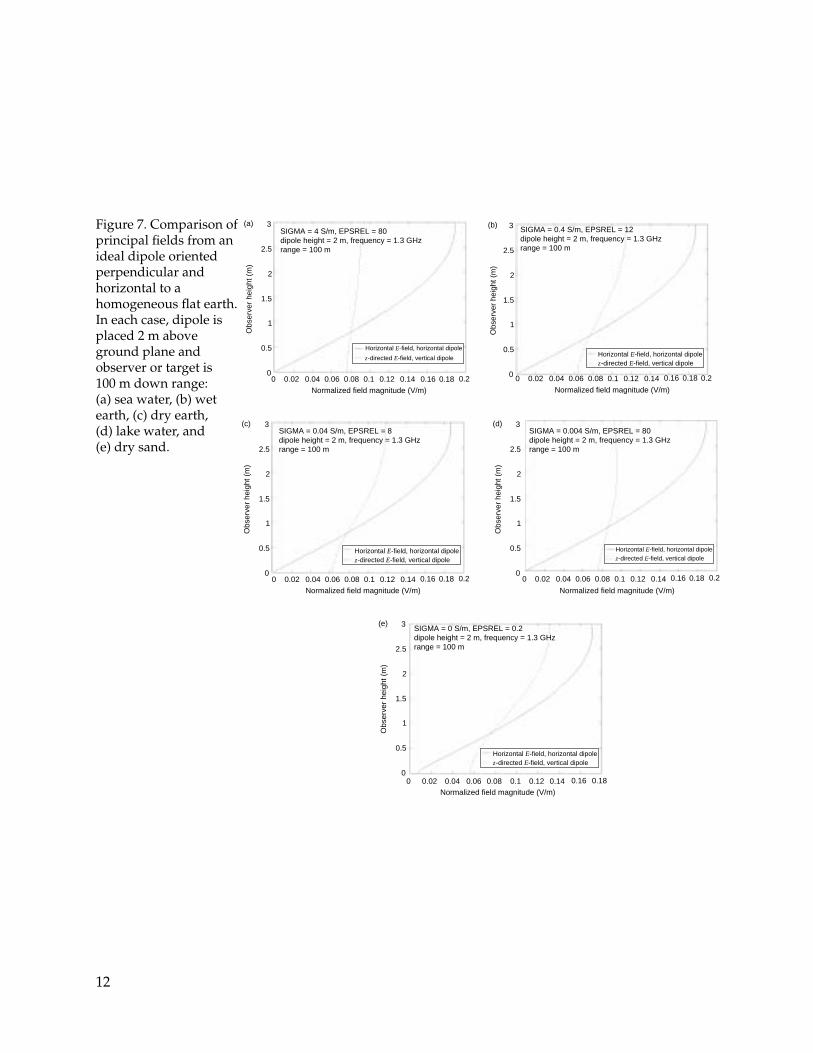
Figure 7. Comparison ofprincipal fields from anideal dipole orientedperpendicular andhorizontal to ahomogeneous flat earth.In each case, dipole isplaced 2 m aboveground plane andobserver or target is100 m down range:(a) sea water, (b) wetearth, (c) dry earth,(d) lake water, and(e) dry sand.

0 0.02 0.04 0.06 0.08 0.1 0.12 0.14 0 0.02 0.04 0.06 0.08 0.1 0.12 0.14 0.16 0.18

0 0.02 0.04 0.06 0.08 0.1 0.12 0.14

0 0.02 0.04 0.06 0.08 0.1 0.12 0.14 0.16 0.18

0 0.02 0.04 0.06 0.08 0.1 0.12 0.14 0.16 0.18 0.2 0.16 0.18 0.2

0

0.5

1

1.5

2

2.5

3


Obs

erve

r he

ight

(m

)

(a)

0

0.5

1

1.5

2

2.5

3


Obs

erve

r he

ight

(m

)

(d)

0

0.5

1

1.5

2

2.5

3


Obs

erve

r he

ight

(m

)

(e)

0

0.5

1

1.5

2

2.5

3


Obs

erve

r he

ight

(m

)

(c)

0

0.5

1

1.5

2

2.5

3


Obs

erve

r he

ight

(m

)

(b)SIGMA = 4 S/m, EPSREL = 80dipole height = 2 m, frequency = 1.3 GHzrange = 100 m

Horizontal E-field, horizontal dipole

z-directed E-field, vertical dipole

SIGMA = 0.4 S/m, EPSREL = 12dipole height = 2 m, frequency = 1.3 GHzrange = 100 m


SIGMA = 0 S/m, EPSREL = 0.2dipole height = 2 m, frequency = 1.3 GHzrange = 100 m


0.16 0.18 0.2 0.2





12

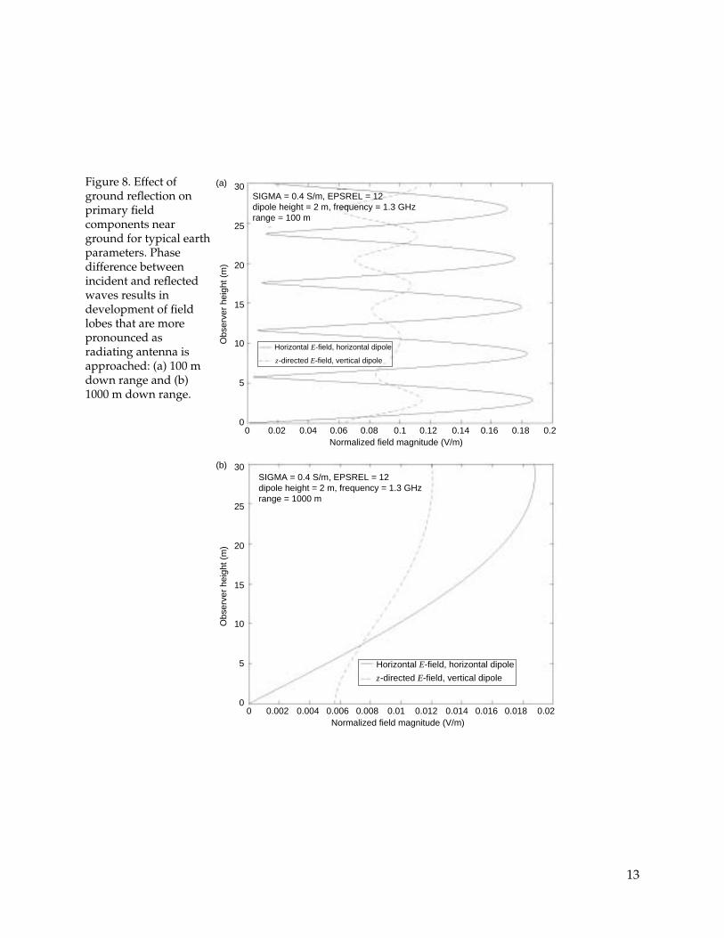
Figure 8. Effect ofground reflection onprimary fieldcomponents nearground for typical earthparameters. Phasedifference betweenincident and reflectedwaves results indevelopment of fieldlobes that are morepronounced asradiating antenna isapproached: (a) 100 mdown range and (b)1000 m down range.

0 0.02 0.04 0.06 0.08 0.1 0.12 0.14 0.16 0.18 0.20

5

10

15

20

25

30


0 0.002 0.004 0.006 0.008 0.01 0.012 0.014 0.016 0.018 0.020

5

10

15

20

25

30


Obs

erve

r he

ight

(m

)O

bser

ver

heig

ht (

m)

(a)

(b)SIGMA = 0.4 S/m, EPSREL = 12dipole height = 2 m, frequency = 1.3 GHzrange = 1000 m






13

3. Conclusion

A suite of MATLAB m-files have been developed to calculate the electro-magnetic fields produced by a vertical and a horizontal infinitesimal unitdipole over a homogeneous flat (ground) plane. Calculations for the fieldsabove the ground plane have been made for various ground-plane conduc-tivities and relative dielectric constants. The calculations bound the practi-cal range of parameters representative of natural earth terrain.

For a frequency of 1.3 GHz, where the dipole and the observer are close tothe ground plane (<3 m), significant difference is seen in the magnitude ofthe fields from either dipole orientation. The power density on target willbe much larger for vertical dipole orientation. The effects of rough terrain,foliage, or scattering from manmade or natural objects in the path from thedipole to target may alter this conclusion. How these other scatterers mightaffect the field structure at a target at 1.3 GHz is not known at this time. Ifthe effects are random in nature, the present conclusion is most likely stillvalid. From the simple, smooth, flat ground model, then, one must con-clude that vertical polarization (antenna radiating a vertically polarizedfield) will deliver the most energy to the target. Unless the target’s pref-erence for field orientation for maximum pickup is known, a vertically po-larized antenna may in fact be the best choice for a ground weapon system.

14

References

Abramowitz, M., and I. A. Stegun, Handbook of Mathematical Functions, Na-tional Bureau of Standards, Applied Mathematics Series–55, U.S. Depart-ment of Commerce (1970).

Banos, A., Dipole Radiation in the Presence of a Conducting Half-Space, Perga-mon, Oxford (1966).

Chase, R., MATLAB m-file, Plasma Dispersion Function with Complex Argu-ment (unpublished).

Collin, R. E., Antenna and Radiowave Propagation, McGraw-Hill, New York(1985).

Collin, R. E., and F. J. Zucker, Antenna Theory, Part 1, McGraw-Hill, NewYork (1969).

King, R.W.P., and S. S. Sandler, “The electromagnetic field of a vertical elec-tric dipole over the earth or sea,” IEEE Trans. Antennas Propag. 42, No. 3(March 1994), pp 382–389.

King, R.W.P., M. Owens, and T. T. Wu, Lateral Electromagnetic Waves,Springer-Verlag, New York (1992).

Maclean, T.S.M., and Z. Wu, Radiowave Propagation Over Ground, Chapmanand Hall, London (1993).

MATLAB , release 5.3, The Math Works, Inc., Natick, MA (1984–1999).

Sommerfeld, A., Partial Differential Equations in Physics, Academic Press,New York (1949).

15

16

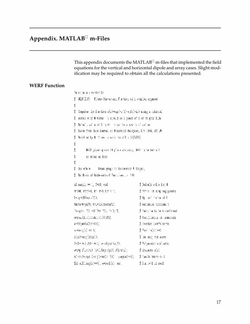
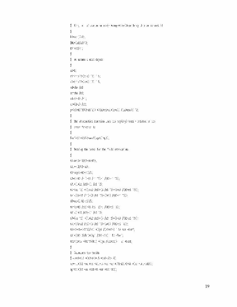
Appendix. MATLAB m-Files

This appendix documents the MATLAB m-files that implemented the fieldequations for the vertical and horizontal dipole and array cases. Slight mod-ification may be required to obtain all the calculations presented.

WERF Functionfunction w = werf(z,N)

% WERF(Z,N) Plasma Dispersion Function with complex argument.

%

% Computes the function w(z)=exp(-z^2)*erfc(-iz) using a rational

% series with N terms. N should be a power of 2 or it gets SLOW.

% Default value of N is 64. z can be a matrix of values.

% Taken from Siam Journal on Numerical Analysis, Oct 1994, V31,#5.

% Modified by R. Chase to work for all z (4/3/95).

%

% N=32 gives approx 14 place accuracy, N=64 is better and

% it seems as fast.

%

% See wfn.m -- Draws graph in Abramowitz & Stegun,

% Handbook of Mathematical Functions, p. 298

if nargin == 1, N=64; end % Default value for N

M=2*N; M2=2*M; k=[-M+1:1:M-1]'; % M2=no. of sampling points

L=sqrt(N/sqrt(2)); % Optimal choice of L

theta=k*pi/M; t=L*tan(theta/2); % Variables thetaand t

f=exp(-t.^2).*(L^2+t.^2); f=[0;f]; % function to be transformed

a=real(fft(fftshift(f)))/M2; % Coefficients of transform

a=flipud(a(2:N+1)); % Reorder coefficients

nz=imag(z) <= 0; % Find im(z) <=0

z(nz)=conj(z(nz)); % Use conj for above

Z=(L+i*z)./(L-i*z); p=polyval(a,Z); % Polynomial evaluation

w=2*p./(L-i*z).^2+(1/sqrt(pi))./(L-i*z); % Evaluate w(z)

w(nz)=2*exp(-(conj(z(nz)).^2)) - conj(w(nz)); % Handle im(z) <= 0

%if all(imag(z)==0), w=real(w); end % Rtn real if real

17

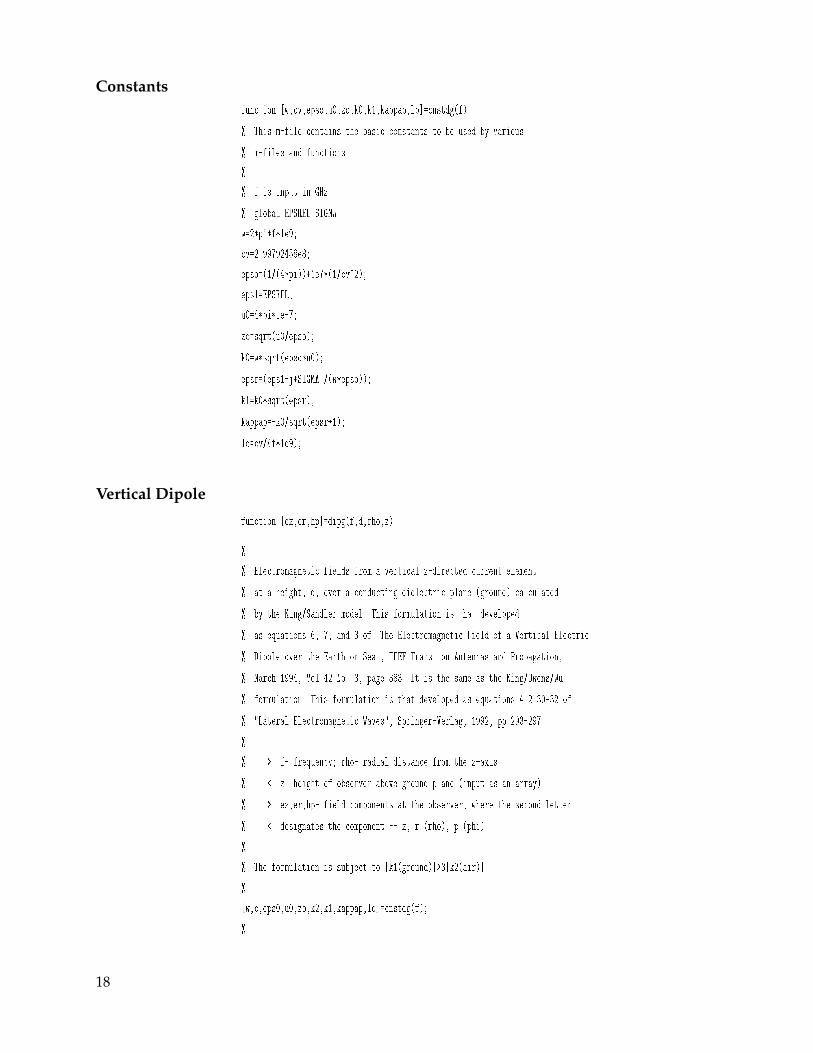
Constantsfunction [w,cv,epso,u0,zo,k0,k1,kappap,lo]=cnstdg(f)

% This m-file contains the basic constants to be used by various

% m-files and functions

%

% f is input in GHz

% global EPSREL SIGMA

w=2*pi*f*1e9;

cv=2.99792458e8;

epso=(1/(4*pi))*1e7*(1/cv^2);

eps1=EPSREL;

u0=4*pi*1e-7;

zo=sqrt(u0/epso);

k0=w*sqrt(epso*u0);

epsr=(eps1-j*SIGMA./(w*epso));

k1=k0*sqrt(epsr);

kappap=-k0/sqrt(epsr+1);

lo=cv/(f*1e9);

Vertical Dipole

function [ez,er,hp]=dipg(f,d,rho,z)

%

% Electromagnetic fields from a vertical z-directed current element

% at a height, d, over a conducting dielectric plane (ground) calculated

% by the King/Sandler model. This formulation is that developed

% as equations 6, 7, and 8 of "The Electromagnetic Field of a Vertical Electric

% Dipole over the Earth or Sea", IEEE Trans. on Antennas and Propagation,

% March 1994, Vol 42 No. 3, page 383. It is the same as the King/Owens/Wu

% formulation. This formulation is that developed as equations 4.2.30-32 of

% "Lateral Electromagnetic Waves", Springer-Verlag, 1992, pp 293-297.

%

% > f- frequency; rho- radial distance from the z-axis

% < z- height of observer above ground plane (input as an array)

% > ez,er,hp- field components at the observer, where the second letter

% < designates the component -- z, r (rho), p (phi)

%

% The formulation is subject to |k1(ground)|>3|k2(air)|

%

[w,c,eps0,u0,zo,k2,k1,kappap,lo]=cnstdg(f);

%

18

% King, et. al assume an exp(-i*omega*time)dependency thus we convert k1

%

k1=conj(k1);

%N2=(k1/k2)^2;

k21=k2/k1;

%

% We assume a unit dipole

%

il=1;

r1=(rho^2+(z-d).^2).^.5;

r2=(rho^2+(z+d).^2).^.5;

sd=rho./r1;

sr=rho./r2;

cd=(z-d)./r1;

cr=(d+z)./r2;

p=(r2*k2^3/(2*k1^2)).*((k2*r2+k1*(z+d))./(k2*rho)).^2;

%

% The attenuation function less the exp(i*p) term - related to the

% error function is

%

Ferf=((1+i)/4)*werf(sqrt(i*p));

%

% Develop the terms for the field expressions

%

t1=w*u0*il/(2*pi*k2);

t11=-il/(2*pi);

t2=exp(i*k2*r1)/2;

t3=(i*k2./r1)-(1./r1.^2)-i./(k2*r1.^3);

t31=(i*k2./r1)-(1./r1.^2);

t4=(cd.^2).*((i*k2./r1)-(3./r1.^2)-(3*i)./(k2*r1.^3));

t41=((i*k2./r1)-(3./r1.^2)-(3*i)./(k2*r1.^3));

t5=exp(i*k2*r2)/2;

t6=(i*k2./r2)-(1./r2.^2)-i./(k2*r2.^3);

t61=(i*k2./r2)-(1./r2.^2);

t7=(cr.^2).*((i*k2./r2)-(3./r2.^2)-(3*i)./(k2*r2.^3));

t71=((i*k2./r2)-(3./r2.^2)-(3*i)./(k2*r2.^3));

t8=(2*t5*(k2^3)/k1).*((pi./(k2*r2)).^.5).*sr.*Ferf;

t81=((k2^3)/k1)*((pi./(k2*r2)).^.5).*Ferf;

t82=(2*t5.*(k2^3)/k1).*((pi./(k2*r2)).^.5).*Ferf;

%

% Calculate the fields

% ez=t1*(t2.*(t3-t4)+t5.*(t6-t7)-t8);

er=-t1*(t2.*sd.*cd.*t41+t5.*sr.*cr.*t71-k21*2*t5.*(sr.*t61-t81));

hp=t11*(t2.*sd.*t31+t5.*sr.*t61-t82);

19

Horizontal Dipole

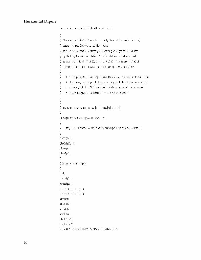
function [ez,ep,er,hz,hp,hr]=dipgh(f,d,phi,rho,z)

%

% Electromagnetic fields from a horizontally directed (perpendicular to z)

% current element located in the phi=0 plane

% at a height, d, over a conducting dielectric plane (ground) calculated

% by the King/Owens/Wu formulation. This formulation is that developed

% as equations 7.10.75, 7.10.80, 7.10.84, 7.10.92, 7.10.93 and 7.10.94 of

% "Lateral Electromagnetic Waves", Springer-Verlag, 1992, pp 293-297.

%

% > f- frequency(GHz); phi- angle about the z-axis, rho- radial distance from

% < the z-axis, z- height of observer above ground plane (input as an array)

% > ez,ep,er,hz,hp,hr- field components at the observer, where the second

% < letter designates the component -- z, r (rho), p (phi)

%

%

% The formulation is subject to |k1(ground)|>3|k2(air)|

%


%

% King, et. al assume an exp(-i*omega*time)dependency thus we convert k1

%

k1=conj(k1);

%N2=(k1/k2)^2;

k21=k2/k1;

k2p=k2/rho;

%

% We assume a unit dipole

%

il=1;

cp=cos(phi);

sp=sin(phi);

r1=(rho^2+(z-d).^2).^.5;

r2=(rho^2+(z+d).^2).^.5;

sd=r1/rho;

sdo=1./sd;

sr=r2/rho;

sro=1./sr;

cd=(z-d)./r1;

cr=(d+z)./r2;

p=(r2*k2^3/(2*k1^2)).*((k2*r2+k1*(z+d))./(k2*rho)).^2;

20

%

% The attenuation function less the exp(i*p) term - related to the

% error function is

% Ferf=((1+i)/4)*werf(sqrt(i*p));

%

% Develop the terms for the field expressions

%

t1=w*u0*il*cp/(4*pi*k2);

t11=-w*u0*il*sp/(4*pi*k2);

t12=il*sp/(4*pi);

t13=il*cp/(4*pi);

t2=exp(i*k2*r1);

t32=(i*k2./r1)-(1./r1.^2)-i./(k2*r1.^3);

t3=(2./r1.^2)+2*i./(k2*r1.^3);

t31=(i*k2./r1)-(1./r1.^2);

t4=(cd.^2).*((i*k2./r1)-(3./r1.^2)-(3*i)./(k2*r1.^3));

t41=(cd).*((i*k2./r1)-(3./r1.^2)-(3*i)./(k2*r1.^3));

t5=exp(i*k2*r2);

t62=(i*k2./r2)-(1./r2.^2)-i./(k2*r2.^3);

t6=(2./r2.^2)+2*i./(k2*r2.^3);

t61=(i*k2./r2)-(1./r2.^2);

t7=(cr.^2).*((i*k2./r2)-(3./r2.^2)-(3*i)./(k2*r2.^3));

t71=(cr).*((i*k2./r2)-(3./r2.^2)-(3*i)./(k2*r2.^3));

t72=((1./r2.^2)+(3*i)./(k2*r2.^3)-3./((k2^2)*r2.^4));

t73=(cr.^2).*((i*k2./r2)-(6./r2.^2)-(15*i)./(k2*r2.^3));

t8=((k2^3)/k1)*((pi./(k2*r2)).^.5).*sr.*Ferf;

t81=((k2^3)/k1)*((pi./(k2*r2)).^.5).*Ferf;

t82=(2*t5*(k2^3)/k1).*((pi./(k2*r2)).^.5).*Ferf;

t83=((pi./(k2*r2)).^.5).*Ferf;

%

% Calculate the fields

%

ez=t1*(-t2.*sdo.*t41+t5.*sro.*t71-2*k21*t5.*(sro.*t61-t81));

er=t1*(t2.*(t3+t4)-t5.*(t6+t7-2*k21*t61+2*(k21^2)*(t62-t8)));

ep=t11*(t2.*t32-t5.*t62-t5.*(-2*k21*cr.*t61+2*(k21^2)*(t6+t7)...

+2*i*k21^3*k2p*(sr.^2).*t83));

hr=t12*(t2.*cd.*t31-t5.*cr.*t61+2*k21*t5.*(t6+i*k21*k2p*(sr.^2).*t83+t7));

hp=t13*(t2.*cd.*t31-t5.*cr.*t61+2*k21*t5.*(t62-k21*(k2^2)*(sr).*t83));

hz=t12*(t2.*sdo.*t31-t5.*sro.*t61+2*sro.*t5.*(k21*t71(k21^2)*(t72+t73)));

21

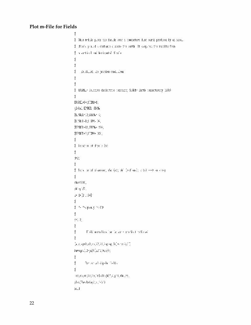
Plot m-File for Fields%

% This m-file plots the fields over a conductive flat earth produced by an ideal

% dipole placed a distance d above the earth. It compares the results from

% a vertical and horizontal dipole.

%

%

% Establish the problem conditions

%

%

% EPSREL- Relative dielectric constant; SIGMA- Earth conductivity (S/m)

%

EPSREL=80;SIGMA=4;

global EPSREL SIGMA

%EPSREL=12;SIGMA=.4;




%

% Location of dipole (m)

%

d=2;

%

% Location of observer, rho (m); phi (radians); z (m) ---> an array

%

rho=1000;

phi=pi/2;

z=.1*[1:1:30];

%

% f- frequency in GHz

%

f=1.3;

%

% Field normalization factor - one Watt radiated

%


Fn=sqrt(12*pi/((k2^2)*zo));

%

% Horizontal dipole fields

%

[ez,ep,er,hz,hp,hr]=dipgh(f,d,phi,rho,z);

plot(Fn*abs(ep),z,'-b')

hold

22

%

% Vertical dipole fields

%

[ezv,erv,hpv]=dipg(f,d,rho,z);

plot(Fn*abs(ezv),z,'-.r')

ts=Fn*abs(erv(1));

title('Vertical and Horizontal Ideal Dipole fields over Ground')

text(ts,z(19),['SIGMA = ',num2str(SIGMA),' S/m EPSREL=

',num2str(EPSREL)])

text(ts,z(18),['Dipole height = ',num2str(d),' meters; Frequency =

',num2str(f),' GHz'])

text(ts,z(17),['Range = ',num2str(rho),' meters'])

ylabel('Observer height - meters')

xlabel('Normalized field magnitude - V/m')

legend('Horizontal E-field, horizontal dipole','z-directed E-field,

vertical dipole')

hold

Fresnel Reflection Coefficients and Plotsfunction [rcomv,rcomh]=Fresnel1(f,psi)

%

% This routine calculates the Fresnel reflection coefficients for

% vertical and horizontal incident fields

%

% after Collin, "Antenna and Radiowave Propagation", page 345

%

% f-frequency in GHz; psi- array of incident angles

%

% Code returns the arrays rcomv and rcomh, the vertical and horizontal

% complex reflection coefficients, respectively.

%

global EPSREL SIGMA

w=2*pi*f*1e9;

cv=2.99792458e8;

epso=(1/(4*pi))*1e7*(1/cv^2);

epsr=(EPSREL-j*SIGMA./(w*epso));

rcomv=(epsr*sin(psi)-sqrt(epsr-cos(psi).^2))./(epsr*sin(psi)+sqrt(epsr-cos(psi).^2));

rcomh=(sin(psi)-sqrt(epsr-cos(psi).^2))./(sin(psi)+sqrt(epsr-cos(psi).^2));

+++++++++++++++++++++++++++++++++++++++++++++++++++++++++++++++++++++++++++++++++++++++++++++++++++

%

23

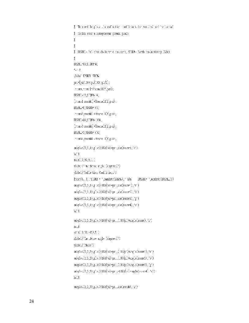
% This m-file plots the reflection coefficient for vertical and horizontal

% fields over a homogeneous ground plane

%

%

% EPSREL- Relative dielectric constant; SIGMA- Earth conductivity (S/m)

%

EPSREL=80;SIGMA=4;

f=1.3;

global EPSREL SIGMA

psi=[pi/1000:pi/1000:pi/2];

[rcomv,rcomh]=Fresnel1(f,psi);

EPSREL=12;SIGMA=.4;

[rcomv1,rcomh1]=Fresnel1(f,psi);

EPSREL=8;SIGMA=.04;


EPSREL=80;SIGMA=.004;


EPSREL=2;SIGMA=.000;


subplot(2,2,1),plot((180/pi)*psi,abs(rcomv),'k')

hold

axis([0,90,0,1])

xlabel('Incidence angle (degrees)')

ylabel('Reflection Coefficient')

%text(5,.8,['SIGMA = ',num2str(SIGMA),' S/m EPSREL= ',num2str(EPSREL)])

subplot(2,2,1),plot((180/pi)*psi,abs(rcomv1),'r')

subplot(2,2,1),plot((180/pi)*psi,abs(rcomv2),'b')

subplot(2,2,1),plot((180/pi)*psi,abs(rcomv3),'g')

subplot(2,2,1),plot((180/pi)*psi,abs(rcomv4),'c')

hold

subplot(2,2,2),plot((180/pi)*psi,(180/pi)*angle(rcomv),'k')

hold

axis([0,90,-190,5])


ylabel('Phase')

subplot(2,2,2),plot((180/pi)*psi,(180/pi)*angle(rcomv1),'r')

subplot(2,2,2),plot((180/pi)*psi,(180/pi)*angle(rcomv2),'b')

subplot(2,2,2),plot((180/pi)*psi,(180/pi)*angle(rcomv3),'g')

subplot(2,2,2),plot((180/pi)*psi,-(180/pi)*angle(rcomv4),'c')

hold

subplot(2,2,3),plot((180/pi)*psi,abs(rcomh),'k')

24

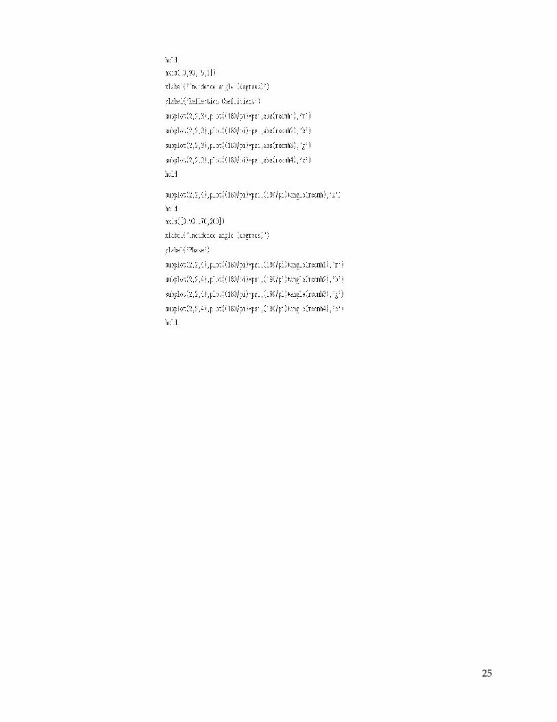
hold

axis([0,90,.5,1])


ylabel('Reflection Coefficient')

subplot(2,2,3),plot((180/pi)*psi,abs(rcomh1),'r')

subplot(2,2,3),plot((180/pi)*psi,abs(rcomh2),'b')

subplot(2,2,3),plot((180/pi)*psi,abs(rcomh3),'g')

subplot(2,2,3),plot((180/pi)*psi,abs(rcomh4),'c')

hold

subplot(2,2,4),plot((180/pi)*psi,(180/pi)*angle(rcomh),'k')

hold

axis([0,90,170,200])


ylabel('Phase')

subplot(2,2,4),plot((180/pi)*psi,(180/pi)*angle(rcomh1),'r')

subplot(2,2,4),plot((180/pi)*psi,(180/pi)*angle(rcomh2),'b')

subplot(2,2,4),plot((180/pi)*psi,(180/pi)*angle(rcomh3),'g')

subplot(2,2,4),plot((180/pi)*psi,(180/pi)*angle(rcomh4),'c')

hold

25

26

27

Distribution

AdmnstrDefns Techl Info CtrATTN DTIC-OCP8725 John J Kingman Rd Ste 0944FT Belvoir VA 22060-6218

DARPAATTN S Welby3701 N Fairfax DrArlington VA 22203-1714

Ofc of the Secy of DefnsATTN ODDRE (R&AT)The PentagonWashington DC 20301-3080

Ofc of the Secy of DefnsATTN OUSD(A&T)/ODDR&E(R) R J Trew3080 Defense PentagonWashington DC 20301-7100

AMCOM MRDECATTN AMSMI-RD W C McCorkleRedstone Arsenal AL 35898-5240

US Army TRADOCBattle Lab Integration & Techl DirctrtATTN ATCD-BATTN ATCD-B J A KleveczFT Monroe VA 23651-5850

US Military AcdmyMathematical Sci Ctr of ExcellenceATTN MADN-MATH MAJ M HuberThayer HallWest Point NY 10996-1786

Dir for MANPRINTOfc of the Deputy Chief of Staff for PrsnnlATTN J HillerThe Pentagon Rm 2C733Washington DC 20301-0300

SMC/CZA2435 Vela Way Ste 1613El Segundo CA 90245-5500

TECOMATTN AMSTE-CLAberdeen Proving Ground MD 21005-5057

US Army ARDECATTN AMSTA-AR-TDBldg 1Picatinny Arsenal NJ 07806-5000

US Army Info Sys Engrg CmndATTN AMSEL-IE-TD F JeniaFT Huachuca AZ 85613-5300

US Army Natick RDEC Acting Techl DirATTN SBCN-T P BrandlerNatick MA 01760-5002

US Army Natl Ground Intllgnc CtrATTN IAFSTC-RMA T Caldwell220 Seventh St NECharlottesville VA 22901-5396

US Army Nuc & Chem AgcyATTN MONA-NU R Pfeffer7150 Heller Loop Rd Ste 101Springfield VA 22150

US Army Simulation Train & InstrmntnCmnd

ATTN AMSTI-CG M MacedoniaATTN J Stahl12350 Research ParkwayOrlando FL 32826-3726

US Army TACOMATTN ATSTA-OE E Di VitoWarren MI 48397-5000

US Army Tank-Automtv Cmnd RDECATTN AMSTA-TR J ChapinWarren MI 48397-5000

Nav Air Warfare Ctr Aircraft DivATTN E3 Div S Frazier Code 5.1.7Unit 4 Bldg 966Patuxent River MD 20670-1701

Distribution (cont’d)

28

Nav Rsrch LabATTN Code 6650 T Wieting4555 Overlook Ave SWWashington DC 20375-5000

Nav Surfc Warfare CtrATTN Code B07 J Pennella17320 Dahlgren Rd Bldg 1470 Rm 1101Dahlgren VA 22448-5100

Nav Surfc Warfare CtrATTN Code F-45 D StoudtATTN Code F-45 S MoranATTN Code J-52 W LucadoDahlgren VA 22448-5100

Air Force Rsrch Lab (Phillips Ctr)ATTN AFRL/WST W WaltonATTN AFRL W L Baker Bldg 413ATTN WSM P Vail3550 Aberdeen Ave SEKirtland NM 87112-5776

CIAATTN OSWR J F PinaWashington DC 20505

Federal Communications CommissionOffice of Eng and TechnlATTN Rm 7-A340 R Chase445 12th Stret SWWashington DC 20554

Hicks & Assoc IncATTN G Singley III1710 Goodrich Dr Ste 1300McLean VA 22102

Pacific Northwest Natl LabATTN K8-41 R ShippellPO Box 999Richland WA 99352

Palisades Inst for Rsrch Svc IncATTN E Carr1745 Jefferson Davis Hwy Ste 500Arlington VA 22202-3402

SpartaATTN R O’Connor4901 Corporate Dr Ste 102Huntsville AL 35805-6257

DirectorUS Army Rsrch LabATTN AMSRL-RO-D JCI ChangATTN AMSRL-RO-EN W D BachPO Box 12211Research Triangle Park NC 27709

US Army Rsrch LabATTN AMSRL-DD J M MillerATTN AMSRL-D D R SmithATTN AMSRL-CI-AI-R Mail & Records

MgmtATTN AMSRL-CI-AP Techl Pub (2 copies)ATTN AMSRL-CI-LL Techl Lib (2 copies)ATTN AMSRL-SE-DP M LitzATTN AMSRL-SE-DP R A Kehs (3 copies)ATTN AMSRL-SE-DS J Miletta (10 copies)ATTN AMSRL-SE-DS J Tatum (5 copies)ATTN AMSRL-SE-DS M BerryATTN AMSRL-SE-DS W O CoburnAdelphi MD 20783-1197

1. AGENCY USE ONLY

8. PERFORMING ORGANIZATION REPORT NUMBER

7. PERFORMING ORGANIZATION NAME(S) AND ADDRESS(ES)

12a. DISTRIBUTION/AVAILABILITY STATEMENT

10. SPONSORING/MONITORING AGENCY REPORT NUMBER

5. FUNDING NUMBERS4. TITLE AND SUBTITLE

6. AUTHOR(S)

REPORT DOCUMENTATION PAGE

3. REPORT TYPE AND DATES COVERED2. REPORT DATE

11. SUPPLEMENTARY NOTES

14. SUBJECT TERMS

13. ABSTRACT (Maximum 200 words)

Form ApprovedOMB No. 0704-0188

(Leave blank)

9. SPONSORING/MONITORING AGENCY NAME(S) AND ADDRESS(ES)

Public reporting burden for this collection of information is estimated to average 1 hour per response, including the time for reviewing instructions, searching existing data sources,gathering and maintaining the data needed, and completing and reviewing the collection of information. Send comments regarding this burden estimate or any other aspect of thiscollection of information, including suggestions for reducing this burden, to Washington Headquarters Services, Directorate for Information Operations and Reports, 1215 JeffersonDavis Highway, Suite 1204, Arlington, VA 22202-4302, and to the Office of Management and Budget, Paperwork Reduction Project (0704-0188), Washington, DC 20503.

12b. DISTRIBUTION CODE

15. NUMBER OF PAGES

16. PRICE CODE

17. SECURITY CLASSIFICATION OF REPORT

18. SECURITY CLASSIFICATION OF THIS PAGE

19. SECURITY CLASSIFICATION OF ABSTRACT

20. LIMITATION OF ABSTRACT

NSN 7540-01-280-5500 Standard Form 298 (Rev. 2-89)Prescribed by ANSI Std. Z39-18298-102

Propagation of Electromagnetic Fields Over Flat Earth

February 2001 Summary, Oct 99 to Sept 00

This report looks at the interaction of radiated electromagnetic fields with earth ground in military or law- enforcement applications of high-power microwave (HPM) systems. For such systems to be effective, themicrowave power density on target must be maximized. The destructive and constructive scattering of the fields as they propagate to the target will determine the power density at the target for a given source. The question of field polarization arises in designing an antenna for an HPM system. Should the transmitting antenna produce vertically, horizontally, or circularly polarized fields? Which polarization maximizes the power density on target? This report provides a partial answer to these questions. The problems of calculating the reflection of uniform plane wave fields from a homogeneous boundary and calculating the fields from a finite source local to a perfectly conducting boundary are relatively straightforward. However, when the source is local to a general homogeneous plane boundary, the solution cannot be expressed in closed form. An approximation usually of the form of an asymptotic expansion results. Calculations of the fields are provided for various source and target locations for the frequencies of interest. The conclusion is drawn that the resultant vertical field from an appropriately oriented source antenna located near and above the ground can be significantly larger than a horizontally polarized field radiated from the same location at a 1.3 GHz frequency at observer locations near and above the ground.

Antenna, ground interaction

Unclassified

ARL-TR-2352

0NE6YY622705.H94

AH9462705A

ARL PR:AMS code:

DA PR:PE:

Approved for public release; distributionunlimited.

Unclassified Unclassified

2800 Powder Mill RoadAdelphi, MD 20783-1197

U.S. Army Research LaboratoryAttn: AMSRL-SE-DS [email protected]

U.S. Army Research Laboratory

Joseph R. Miletta

email:2800 Powder Mill RoadAdelphi, MD 20783-1197

33

UL

29

Documents

Propagation of Electromagnetic Fields Over Flat Earth of Electromagnetic Fields Over Flat Earth ARL-TR-2352 February 2001 Joseph R. Miletta Approved for public release; distribution