Embed Size (px)
Citation preview

NLR-TP-2000-302
Propagation lifetime calculation of the P&WPropagation lifetime calculation of the P&WPropagation lifetime calculation of the P&WPropagation lifetime calculation of the P&Wcompressor fan disccompressor fan disccompressor fan disccompressor fan discLife prediction based on crack growth
O. Kogenhop

NationaalNationaalNationaalNationaal Lucht- en Ruimtevaartlaboratorium Lucht- en Ruimtevaartlaboratorium Lucht- en Ruimtevaartlaboratorium Lucht- en RuimtevaartlaboratoriumNational Aerospace Laboratory NLR
NLR-TP-2000-302
Propagation lifetime calculation of the P&WPropagation lifetime calculation of the P&WPropagation lifetime calculation of the P&WPropagation lifetime calculation of the P&Wcompressor fan disccompressor fan disccompressor fan disccompressor fan discLife prediction based on crack growth
O. Kogenhop
This investigation has been carried out as a Master’s thesis for the Delft University ofTechnology, faculty Mechanical Engineering and Marine Engineering, section Process andEnergy with main subject Gas Turbines. The investigation has been carried out undersupervision of prof. ir. J.P. van Buijtenen and ir. T. Tinga.
The contents of this report may be cited on condition that full credit is given to NLR andthe author.
Division: Structures and MaterialsIssued: 31 May 2000Classification of title: Unclassified


- 3 -NLR-TP-2000-302
Summary
The main object of this report is to investigate whether it is possible to determine the propagation
lifetime for complicated gas turbine components by performing crack growth calculations. Therefore
a certain calculation course/strategy is necessary, which will be shown in this report. As a case study
the present�����
-stage fan disc of a Pratt & Whitney engine of the RNLAF F16 is used. This fan disc
is part of a three-stage rotor fan, and provides the transmission of the loads through an attached hub to
the outer (low-pressure) shaft. This disc has been known to show cracks that develop from the thrust
balance holes in the hub.
The key elements in the strategy are: investigation of the load spectrum, determination of the load
sequence, investigation of the materials’ crack growth properties, determination of the stress intensity
factor solution, and the determination of a start- and stop criterion. The loads on the�����
-stage fan
disc are investigated. The main loads are the loads due to torsion and due to the axial force of the
blades. In this investigation the torsion loads are determined with the use of a dynamic gas turbine
program, GSP. Real mission data from the RNLAF is used as input for GSP. A random generator
program is used to create a load sequence file from this data, where the diversification of missions the
RNLAF flies and the mission mix are taken into account. A damage tolerance materials handbook is
used to provide the necessary crack growth data for the crack growth rate relation, which is a function
that describes the crack growth behaviour. The stress intensity factor solution is determined with the
use of finite elements, because the geometry of the�����
-stage fan disc is too complex to be described
by infinite plate solutions. Finally an effort is taken to determine the present stop criterion. As start
criterion the initial crack size Pratt & Whitney uses is used. These aspects are implemented in a crack
growth calculation program, which determines the propagation lifetime.
The results of the propagation lifetime calculations using the critical crack sizes from Pratt & Whitney
look promising. Same lifetimes are obtained for the larger critical crack sizes.
The results also show that the crack growth relation plays a significant role in the lifetime calculation.
The fit constants obtained with the fit of the crack growth data seem to have large inaccuracies, which
effects the lifetime calculation. The main conclusion of this report is that actual life predictions,
for other components, can be performed when accurate material data, load sequence, stress intensity
factor solution, and initial and critical crack lengths are known. This report shows that with the current
data a reasonable lifetime estimation can be made, even when not all of the data is accurate. Another
conclusion is that in determining the stress intensity factor solution, finite element methods are usefull
tools, and produce stress intensity factor solutions for complex geometries.

- 4 -NLR-TP-2000-302
Samenvatting
Het belangrijkste doel van dit rapport is het onderzoeken of het mogelijk is om voor gecompliceerde
gasturbinecomponenten scheurgroeisommen te maken. Hiervoor is een bepaalde oplosstrategie nodig,
welke in dit rapport zal worden behandeld. Als studieobject zal de tweedetraps fandisk uit de Pratt &
Whitney gasturbine van de F-16 van de Koninklijke Luchtmacht worden gebruikt. De fandisk is een
onderdeel van een drietraps rotorfanmodule, en zorgt voor het overbrengen van belastingen door de
aangehechte naaf (hub) naar de lagedrukas. Van de disk is bekend dat er na verloop van tijd scheuren
ontwikkelen en groeien van de thrust balance holes in de richting van de naaf.
De belangrijkste onderdelen van de oplosstrategie zijn het onderzoeken van het belastingspectrum, de
bepaling van de belastingvolgorde, het onderzoeken van het scheurgroeigedrag van het materiaal, de
bepaling van de spanningsintensiteitsfactor, en de bepaling van een start- en een stopcriterium. De
belastingen op de�����
-traps fandisk worden onderzocht. De belangrijkste belastingen zijn de belasting
ten gevolge van torsie en de belasting ten gevolge van de axiale trekkracht op de schoepen. In dit
onderzoek wordt de torsiebelasting bepaald door gebruik te maken van een dynamisch gasturbine-
rekenprogramma, GSP. Actuele missiedata van de Koninklijke Luchtmacht wordt gebruikt als input
voor GSP. Hiermee wordt met gebruik van een C++ programma een willekeurige belastingsvolgorde
gegenereerd, waarbij rekening gehouden wordt met de verscheidenheid van missies en de missie-mix.
Om het scheurgroeigedrag van het diskmateriaal te beschrijven wordt data uit een ”damage tolerant”-
materiaalhandboek gebruikt. De spanningsintensiteitsoplossing wordt bepaald door gebruik te maken
van een eindige-elementenmodel omdat de�����
-traps fandisk te complex is om de oplossing te bepalen
met gebruik van oneindigeplaatoplossingen. Als laatste is er gezocht naar een criterium waardoor
de scheurgroeiberekening zou moeten worden gestopt. Deze aspecten worden in een scheurgroei
programma geımplementeerd waarmee de propagatielevensduur wordt bepaald.
De resultaten van de scheurgroeiberekening ogen hoopvol als er gebruik wordt gemaakt van kritis-
che scheurlengtes die Pratt & Whitney gebruikt. Voor de grotere scheurlengtes kunnen soortgelijke
levensduren worden verkregen.
Uit de resultaten blijkt dat de beschrijving van het materiaalgedrag een belangrijke rol speelt in de
levensduurbepaling. De fitconstanten in de scheurgroeirelatie blijken onnauwkeurig te zijn, waar-
door de levensduurbepaling onnauwkeuriger wordt. De belangrijkste conclusie van dit rapport is dat
levensduurvoorspellingen op basis van scheurgroei inderdaad gemaakt kunnen worden, mits er vol-
doende (juiste) data bekend is van het materiaal, de belastingvolgorde, spanningsintensiteitsoplossing
en de kritieke en initiele scheurlengtes. Dit rapport toont aan dat met de huidige data, welke niet
in alle gevallen volledig bekend is, soortgelijke levensduurvoorspellingen gemaakt kunnen worden.

- 5 -NLR-TP-2000-302
Een belangrijk hulpmiddel hierin is de bepaling van spanningsintensiteitsoplossingen voor complexe
componenten met behulp van eindige elementen.

- 6 -NLR-TP-2000-302
Contents
List of Symbols, Constants, Indices, and Abbreviations 9
1 Introduction 13
1.1 Background 13
1.2 The research project 13
1.3 Stochastic Fatigue Analysis 14
1.4 Structure of the report 15
2 The F-16, a multi-role fighter aircraft 16
2.1 The Royal Netherlands Air Force 16
2.2 Pratt & Whitney F100-PW-220 turbofan gas turbine 17
2.3 Failure of the second stage fan disc 18
3 Life prediction 20
3.1 Introduction 20
3.2 Fatigue design philosophies 20
3.3 Pratt & Whitney Aircraft life prediction interpretation 21
3.3.1 Safe-Life design philosophy 22
3.3.2 Damage Tolerance design philosophy 23
3.3.3 Retirement For Cause design philosophy 23
3.4 Life prediction for the� ���
-stage fan disc 24
4 Fracture mechanics 25
4.1 Introduction 25
4.2 Failure modes 25
4.3 The stress intensity factor 26
4.4 Fatigue crack propagation 27
4.5 Fatigue loading 27
4.6 Crack growth formulation 28
4.6.1 Individual crack growth formulation 28
4.6.2 Crack growth relations 32
4.7 FE method to determine the SIF 34
5 Research prior to life time calculation 38

- 7 -NLR-TP-2000-302
5.1 Determination of the load spectrum 38
5.1.1 Stresses due to axial force 39
5.1.2 Stresses due to torsional effects 42
5.2 Determination of the crack growth relation of Ti-6-2-4-6 44
5.3 Determination of the SIF solution 47
5.4 Stop criteria for crack growth calculation 50
5.4.1 Exceeding the fracture toughness 51
5.4.2 Exceeding the net yield stress 52
5.4.3 Other rejection reasons 52
5.5 Implementation 52
6 Crack growth calculation results 53
6.1 Results 53
6.2 Discussion of the results 54
7 Conclusions and recommendations 56
7.1 Conclusions 56
7.2 Recommendations 56
8 Discussion 57
9 References 57
4 Tables
24 Figures
Appendix A Stresses and displacements at the crack tip 61
2 Figures
Appendix B Derivation of principal stresses 64
3 Figures
Appendix C Mission overview 67
1 Table
1 Figure

- 8 -NLR-TP-2000-302
Appendix D Derivation of quarter side nodes for crack tip elements 68
1 Figure
Appendix E Stress intensity factor calculation of a central cracked plate 71
2 Tables
3 Figures
Appendix F FEM calculated stress intensity factor figures 75
2 Figures
Appendix G C++ programs 78
Appendix H Fitting crack growth data 90
Appendix I Implementation of CRAC2D elements in NASTRAN input files 91
4 Tables
1 Figure
(94 pages in total)

- 9 -NLR-TP-2000-302
List of Symbols, Constants, Indices, and Abbreviations
Symbols
���� crack length�� ���� intrinsic crack length���� ���� width, height� ��� crack opening function� ���� height� �� normal� �� force� ���� radius� �"!��"# ���� displacement components$ �"%&�(' ���� coordinates
) ��� )+* � )-, � )/. ��� coefficients in crack opening function0 ���� diameter1 2 � � Young’s modulus3 2 � � shear modulus4 ����56 polar moment of inertia7 2 � 98 ���� stress intensity factor7;: ��� stress concentration factor� ��� amount of cycles�=<?> ��� number of cycles at critical crack size�A@ ��� amount of cycles at design life (aircraft)B ��� stress ratioC 2 � � stressD �E�� torqueF ��� calculation factorG G � ���EH�IJ%KIJL?MN rate of crack growthC&OQP(RS � ��� ratio of max applied stress to the flow stress
T ��� constraint factorU �� G angle of twistU�V ��� geometric parameter

- 10 -NLR-TP-2000-302
S 2 � � direct stressW 2 � � shear stressX ��� Poisson’s ratioY ���� radius of curvature
Z ���� amount of crack growthZ � ��� amount of fatigue cyclesZ 7 2 � 8 ���� difference between7 O[P�R
and7 O\V �
Constants
C, n, p, q ��� constants for the crack growth equation
a, b, c, d, e, f ��� fit parameters for the crack growth equation
Indices
c, cr critical
eff effective]initial, or summation mark
th threshold�^_$ maximum� ] � minimum$ �"%&�(' direction of plane normals on which stresses work$9%&�"$�'`�"%�' in the context of stresses the first subscript gives the plane normal direction,
the second subscript gives stress direction (example: W RNa is the shear stress
acting on plane which has a normal in $ -direction, in the positive % -direction)
Abbreviations
CCY Calculated CYcles
CFD Computational Fluid Dynamics
CRAGRO NLR’s modular crack growth program
ESA European Space Agency
FACE Fatigue Analyser & Autonomous Combat Evaluation

- 11 -NLR-TP-2000-302
FE Finite Element
FEM Finite Element Method
GSP Gas turbine Simulation Program
HCF High Cycle Fatigue
IFM Inlet Fan Module
LCF Low Cycle Fatigue
LEFM Linear Elastic Fracture Mechanics
LP Low Pressure
NASA National Aeronautics and Space Administration
NASGRO NASA’s crack growth program
NASTRAN product name of the MacNeal-Schwendler corporation
NLR National Aerospace Laboratory
PATRAN product name of the MacNeal-Schwendler corporation
PW Pratt & Whitney
PWA Pratt & Whitney Aircraft
RNLAF Royal Netherlands Air Force
TAC Total Accumulated Cycles
USAF United States Air Force

- 12 -NLR-TP-2000-302
This page is intentionally left blank

- 13 -NLR-TP-2000-302
1 Introduction
1.1 Background
For the economical use of gas turbines it is important to determine the actual service life of gas
turbine components that are subjected to operational conditions. These days, repair and maintenance
intervals are either determined by engine manufacturers or derived from maintenace intervals of other
users or airforce bases. Engine manufacturers frequently base their calculations on heavy use, so that
a conservative lifetime is obtained. Most parts will be loaded less severe, and will thus be replaced
long before the end of their service life. Airline companies and air forces sometimes base their repair
and maintenance intervals on the intervals supplied by the experiences of other users. The operational
use of the gas turbines usually differs between most users. It would therefore be much more attractive
to base the repair and maintenance inspection intervals on actual usage by monitoring all separate
engines (usage monitoring), which is called on-condition maintenance.
1.2 The research project
The main purpose of this project is to find out whether a propagation lifetime can be calculated for
a complex gas turbine component. As a case study, the propagation lifetime of a�b���
-stage fan disc
of the Pratt & Whitney F100-PW-220 gas turbine is determined. This component is described section
2.3. Although the nomenclature indicates a lifetime calculation of the disc, the actual lifetime of the
hub will be determined. Because this hub is a part of the fan disc, the component is called� ���
-stage
fan disc. To determine the propagation lifetime a certain course, or solution strategy must be fol-
lowed. This project is mainly used to determine the course and see whether it can produce acceptable
solutions, provided that there is enough data known. To determine the propagation lifetime, data like
the initial crack size, the crack growth behaviour, and several other aspects must be investigated. The
main aspects of the research are investigation of:� The load spectrum
The load spectrum that is applied during service must be examined to see which load or com-
bination of loads is the cause of the failure of the compressor fan disc. The load spectrum used
in this calculation will be based on usage data of the Royal Netherlands Air Force (RNLAF),
and will form the base of the crack growth calculation. It is therefore of great importance to
generate a representative load sequence, based on the use of the RNLAF, as input for the crack
growth calculation.� The materials crack growth behaviour
The fan disc material must be analysed to determine a relation between the crack growth ratec G KH G �ed and the load parameter (Z 7
).
- 14 -NLR-TP-2000-302
� The stress intensity factor solution
A stress intensity factor solution (SIF- or7
-solution) relates the stress at the crack tip to the
remote load, based on geometry, load, crack length, and location of the crack. The SIF-solution
will be determined using a simplified finite element (FE) model of the hub of the fan disc.� Stop criterion for the crack growth calculation
Failure or rejection of the component can be the result of different mechanisms. Which mecha-
nism or cause causes the component to fail or be rejected must be investigated.
When these aspects are investigated they can be used to determine a deterministic crack growth life-
time.
1.3 Stochastic Fatigue Analysis
Fatigue analyses are usually performed as deterministic analyses, implying that variability of different
parameters is not taken into account. The elastic modulus of a material for instance, is usually taken as
a constant, but in practice it varies between a minimum and a maximum value. Parameters as material
properties, sizes, loading, etc. are often uncertain and not constant. Dealing with the variability of the
parameters a new kind of analysis, namely the stochastic analysis, is introduced. This type of analysis
gives the deterministic analysis an extra dimension by generating solutions with a probability interval.
Dealing with the uncertainties, a much more probable answer is obtained. [Ref. 1]
The next list of factors is solemnly shown to indicate that there are many uncertainties that could
influence the lifetime calculation. [Ref. 2]
Metallurgical and processing variables
- alloy composition,
- microstructure,
- batch (heat-to-heat variation),
- distribution of alloy elements,
- grain size,
- preferred orientation (texture),
- product form,
- orientation with respect to grain direction,
- heat treatment,
- mechanical or thermal-mechanical treatment,
- residual stress,
- manufacturer.

- 15 -NLR-TP-2000-302
Geometrical variables
- thickness,
- crack geometry,
- component geometry,
- stress concentrations (e.g., the presence of a notch, holes, etc.).
Mechanical variables
- cyclic stress amplitude (B
-ratio),
- loading condition (biaxial load, load transfer, etc.),
- cyclic load frequency, wave form, and hold time,
- load interactions in spectrum loading,
- pre-existing residual stress.
Environmental variables
- type of aggressive environment (gas, liquid, liquid metal, etc.),
- concentration of aggressive species,
- electrochemical potential,
- temperature,
1.4 Structure of the report
The report is divided into 7 main chapters. In the first chapter a brief introduction is given on the
objective and the reason of the project. In the second chapter a brief introduction of the F-16 and
the Pratt & Whitney F-100-PW-220 is given. This section also describes the geometry of the� ���
-
stage fan disc, and the failure of an American gas turbine. Before the actual research is discussed,
some elementary theory of life prediction methods and fracture mechanics will be discussed. Chapter
3 describes the various life prediction philosophies, and the philosophies used by Pratt & Whitney
for the F-100-PW-220 gas turbine. The lifetime calculation is based on crack growth. Therefore the
theory of fracture mechanics is discussed in chapter 4. The actual conducted research is described in
chapter 5, which discusses the various aspects which must be investigated prior to the crack growth
calculation. The results and the discussion of the results are given in chapter 6. Finally conclusions
and recommendations are given in chapter 7.

- 16 -NLR-TP-2000-302
2 The F-16, a multi-role fighter aircraft
2.1 The Royal Netherlands Air Force
In 1974 the department of defence decided to replace the Starfighter of the Royal Netherlands Air
Force (RNLAF) with a modern fighter jet. On the 27th of May 1975 the General Dynamics F-16
Falcon (see figure 1) was chosen to become the fighter for the future. A first order of 84 aircraft
was placed, with an option to expand the fleet with more aircraft. The first two F-16’s were assigned
to Leeuwarden airfield. These two aircraft, a single and a dual seater, assembled by Fokker, were
delivered on the 6th of June 1979. The total fleet of the RNLAF consists of 213 F-16’s. (These will
not be in service at the same time, and includes replacements for the calculated 30 aircraft which
could be lost in peace-time due to failure.) The Starfighter was taken out of service in 1984, and the
NF-5 followed in 1991.
Fig. 1 The General Dynamics F-16 fighter aircraft
During their service the F-16’s have been modernised twice. First, a dragchute was added to the
tailplane, and nowadays the F-16’s receive the Mid Life Update. During the Mid Life Update (MLU)
all electronic systems are replaced, the cockpit is rearranged to increase the user-friendliness, and a
Fatigue Analyzer and Autonomous Combat Evaluation system, FACE, is added. A total of 128 Mid
Life Updated F-16’s remain in service until their successor (possibly the Joint Strike fighter, JSF )
arrives towards the year 2008/2010.
Till then the F-16’s must be operated both economicly and safely. This implies that the current life
must be expanded until the replacements arrive. To meet the safety requirements, the repair and
maintenance schedule has to be altered, and all components, that are likely to fail, have to be revised.
This is applicable to both airframe and engine. Currently the F-16’s are powered by Pratt & Whitney
F100-PW-220 turbofan engines.

- 17 -NLR-TP-2000-302
2.2 Pratt & Whitney F100-PW-220 turbofan gas turbine
The F-16’s of the Royal Netherlands Air Force are equipped with Pratt & Whitney F100-PW-220
turbofan engines, of which a cut away picture is shown in figure 2. To improve the performance of the
gas turbine, i.e. the thermal efficiency, a high pressure ratio is essential. Axial compressors are used to
compress air efficiently, and many compressor stages are needed to obtain a high pressure ratio. The
problem with axial compressors is that if they are operated at low rotational speeds (well below the
design value) the air density in the last few stages is much to low, and blades will stall due to excessive
axial flow velocity. The unstable region (manifested by aerodynamic vibration) is encountered when
a gas turbine is started up or operated at low power. To overcome this problem compressors are
mechanically partitioned into two or more sections. These compressor sections usually operate at
different rotational speeds, so each compressor section will be powered by its own turbine. The low-
pressure compressor is driven by the low-pressure turbine, and the high-pressure compressor is driven
by the high-pressure turbine. This configuration is usually referred to as a twin-spool gas turbine.
[Ref. 3]
Fig. 2 Cut away view of the Pratt & Whitney F100-PW-220
The low-pressure compressor is referred to as the fan. The Inlet Fan Module (IFM) is located at the
front of the F100-PW-220 engine, and delivers compressed air to the high pressure compressor. There
are three rows of rotor blades, two rows of vanes, and one row of inlet guide vanes in the in the fan
module. The first, second and third stage blades are mounted respectively on the first, second and
third stage fan disc. The fhg : -stage and i > � -stage fan disc are bolted to the� ���
-stage fan disc. The� ���-stage fan disc is connected to the low pressure shaft through the hub. Figure 3 shows a half cross
section of the fan module. In the past, the United States Air Force (USAF) experienced an accident
which was due to crack propagation from one of the thrust balance holes in the hub of the� ���
-stage
fan disc.

- 18 -NLR-TP-2000-302
Fig. 3 Fan module of the F100-PW-220
2.3 Failure of the second stage fan disc
To perform a risk assessment analysis, a deterministic analysis must be made first. In addition to the
deterministic analysis a stochastic fatigue analysis can be performed, which wil not be part of this
investigation. Due to some problems with the�����
-stage fan disc of the Pratt & Whitney gas turbine,
RNLAF planned risk assessment analysis for this specific component.
There has been one reported fracture of a� ���
-stage fan disc and hub due to a fatigue crack which
grew from one of the 21 thrust balance holes in the direction of the spline (towards the back of the gas
turbine). The event occurred in a development engine on a ground test stand engine that was subjected
to an accelerated mission test.
The current� ���
-stage fan disc in the F100-PW-220 of the RNLAF is a redesign of the original fan
disc design. In this report the second design (redesign) is used for the deterministic fatigue analysis
for two reasons. The first reason is that the second design is the actual disc in the gas turbines of
the RNLAF. The second, main reason, is that it can be used to prove that calculations like these are
possible to perform. A complementary advantage is that the second design is reasonable simple due
to its relatively simple configuration compared to other designs. If the analysis can be made, more
complicated models can be analysed using the same solution strategy.
- 19 -NLR-TP-2000-302
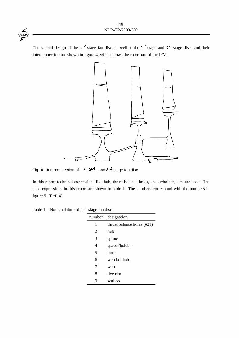
The second design of the� ���
-stage fan disc, as well as the fhg : -stage and i > � -stage discs and their
interconnection are shown in figure 4, which shows the rotor part of the IFM.
Fig. 4 Interconnection of fjg : -, � ��� -, and i > � -stage fan disc
In this report technical expressions like hub, thrust balance holes, spacer/holder, etc. are used. The
used expressions in this report are shown in table 1. The numbers correspond with the numbers in
figure 5. [Ref. 4]
Table 1 Nomenclature of�����
-stage fan disc
number designation
1 thrust balance holes (#21)
2 hub
3 spline
4 spacer/holder
5 bore
6 web bolthole
7 web
8 live rim
9 scallop

- 20 -NLR-TP-2000-302
Fig. 5 Nomenclature of� ���
-stage fan disc
3 Life prediction
3.1 Introduction
Before discussing fracture mechanics, which is the basis for the fatigue lifetime calculation, fatigue
design philosophies will be discussed. Over the years (since the 1950s) several design philosophies
have been developed. The first design philosophy was the traditional safe-life approach. This design
philosophy treats aircraft structures to be designed for a finite service life, during which significant
fatigue damage will not occur. Basic to this approach is that either the structure is not inspectable or
that no inspections are planned during the service life.
3.2 Fatigue design philosophies
Various design philosophies have been developed for dealing with the problem of loss of structural
strength due to the initiation and subsequent growth of cracks by fatigue. In the early 1960s a design
philosophy known as fail-safe was developed. With this philosophy a structure is designed to have an
adequate life free from significant fatigue damage, but continued operation is permitted beyond the
life at which such damage may develop. Safety is incorporated into the fail-safe approach under the
assumption that any fatigue crack that is developed will be detected by routine inspection procedures
before they result in a dangerous reduction of the static strength of the structure. Two requirements

- 21 -NLR-TP-2000-302
cycles
replacement
submacroscopic crack size(S-N sum)SAFE-LIFE
ia
crack lengthpredicted
N DNcr
Fig. 6 Safe-Life design philosophy
are necessary for this approach to be successful. First, a minimum crack size must be defined which
will not go undetected at a routine inspection. Second, a prediction of the crack growth rate until the
next inspection must be defined.
In the early 1970s another design philosophy was proposed. The object of which was to design a
damage tolerant structure. This philosophy is similar to the fail-safe approach, but differs from the
original safe-life approach on two major aspects. First it is assumed that flaws or cracks are present
in the structure as manufactured. These flaws or cracks may arise from metallurgical imperfections in
the material, or from manufacturing faults. The second aspect is that structures may be inspectable or
non-inspectable. This design philosophy is called the damage-tolerance design philosophy.
The application of the damage-tolerance approach to a given component depends on whether the
component is classed as inspectable or non-inspectable during routine service inspections. For com-
ponents that are inspectable the procedures closely follow those used in fail-safe design. However, in
the case of non-inspectable parts it must be demonstrated that the time for the crack to grow to failure,
from the prescribed initial flaw, is greater than the desired service life.
For military gas turbine engines, the majority of components is treated according to the safe-life design
philosophy, so that the components are treated to be free of initial defects or discontinuities and no
planned inspections are going to be done. The USAF and Pratt & Whitney Aircraft use for some of
their components the damage-tolerance design philosophy.
3.3 Pratt & Whitney Aircraft life prediction interpretation
The life prediction according to Pratt & Whitney Aircraft starts with the designation of components
to be either fracture critical or durability critical. The fracture critical designation is used for compo-
nents if its failure results in a total loss of the engine and the inability to continue safe operation of the

- 22 -NLR-TP-2000-302
aircraft. The durability critical designation for components is used when failure of the components
lead to significant maintenance without jeopardising flight safety. All gas turbine components are
subjected to a durability limit calculation. The durability limit (or the economic life limit) presents,
according to Pratt & Whitney, the point in time where it would be more economic to replace a com-
ponent than to continue inspection or repairs. For fracture critical components, also a safety limit is
calculated. This safety limit is considered to be the time beyond which the risk of components failure
is considered to be unacceptably high if corrective actions are not taken. This time is based on the
time required for the maximum probable initial flaw or defect to grow to critical condition and cause
component failure. The safety limit must always be lower than the durability limit and will be used to
determine the inspection intervals. Usually the inspection interval is half the safety limit. In general
the Low Cycle Fatigue (LCF) life limit is used as the durability limit. Several approaches to determine
this life limit exist.
3.3.1 Safe-Life design philosophy
The conventional safe-life design philosophy equals the life limit to the LCF life limit, which is
calculated with the aid of S-N curves (these curves describe the relation between the fatigue life and
the stress level for a given stress concentration factor). The LCF life limit is associated with the time
to initiate a*.", inch long surface crack in a part with no pre-existing defect. The LCF life limit is
determined with the use of a large amount of test data, which gives a distribution of crack initiation
lives. (See figure 6) For the LCF life limit the B.1 value (this is the lifetime wherein 1 out of 1000, or
0.1%, of the test samples a crack has initiated) is used. (See figure 7)
Mean value
Num
ber
of c
ompo
nent
s
LCF
LimitLife
Number of cycles to crack initiation
(B50)
B.1 Initiation Life
Fig. 7 PWA Safe-Life approach

- 23 -NLR-TP-2000-302
3.3.2 Damage Tolerance design philosophy
The initial lifetime calculation (called the initiation life) of the damage tolerance approach is similar
to the calculation following the safe-life approach, but in addition a potential life extension will be
calculated (called the propagation life). This lifetime extension is done by calculating the time for a
crack of minimum detectable NDI size to grow to the critical crack size. The total lifetime will be
calculated as follows:
clknmpo d L ] � MnL ] � ]rqtsvuxw f[y � ]rqz] qz]|{ � k ] � M~} uxw f � � {�� b�_ qz]|{ � k ] � M (1)
The B.1 value of the initiation life is similar to the value used in the safe-life approach. The propaga-
tion life is obtained in a similar way where 1 out of 1000 components has reached the critical crack
length, for which a large amount of test data is necessary. This limit, the B.1 propagation life limit
is also called the safety limit. To actually determine the propagation life several requirements are
needed, such as; service loads, crack propagation rate, critical crack size, initial crack size, and the
stress intensity factor solution.
During service life, inspection intervals are planned. If cracks are found during inspection the con-
cerned component will be rejected and replaced. The first inspection interval is recommended to be
0.5 to 1.0 times the calculated safety limit. If no cracks or flaws are found with the current NDI meth-
ods, the minimal detectable crack or flaw size of the inspection method is assumed to exist. From
this point the inspection interval is also recommended to be 0.5 to 1.0 times the calculated safety
limit. The chance that a component with a crack is found is relatively small because of the B.1 values
of the initiation and propagation life. The initiation life and the propagation life are assumed to be
independent according to Pratt & Whitney Aircraft, so the total risk of finding a cracked component
will be one in a million. If no defects or cracks are found during inspection intervals, but the lifetime
is reached, the component will also be retired. The major disadvantage of the damage tolerance ap-
proach is that most of the components are retired in a premature stage, meaning that the components
are retired in an uncracked state. Due to the high rate of conservatism an additional, third approach,
was developed. (See figure 8)
3.3.3 Retirement For Cause design philosophy
Due to the damage tolerance approach (equation 1) most components are replaced prematurely. This
means that a small part of the potential life capacity of the components is used. The fundamentals of
the retirement for cause approach are based on life extension beyond the LCF life limit of the damage
tolerance approach. This design philosophy does not imply that each individual component can be

- 24 -NLR-TP-2000-302
B.1 Propagation life
failure
Retirement for cause approach
Pred
icte
d cr
ack
leng
th
I
B.1 Initiation life
I
Life
Critical crack size
NDI detection limit
Damage tolerance approach
Safety Limit
Limit
I I Cycles1/2 times safety limit
LCF
Fig. 8 PWA Damage Tolerance and Retirement For Cause approach
used until a crack is detected and that the full life capacity can be used. There are two reasons for
not utilizing the full life capacity. The first reason is that it is possible not to detect internal defects
during inspection. The second reason is that the risk of missing a crack increases with increasing
life. In contrast to the damage tolerance approach, the (risk analysis of the) Pratt & Whitney Aircraft
retirement for cause approach gives the exact risk. At first the maximum acceptable risk is determined
and then a statistical risk analysis is used to calculate how many components may contain a crack
before the whole set of components is retired. Pratt & Whitney Aircraft therefore uses this retirement
for cause approach to increase the LCF life limit, but when a component has reached this limit, it is
retired, whether or not it contains a crack. (See figure 8) [Ref. 5, 6]
3.4 Life prediction for the�����
-stage fan disc
In case of the�����
-stage fan disc the damage tolerant design philosophy is used to perform the life
prediction. The propagation life limit must be determined, which will be based on crack growth from
the initial crack length to the critical crack length.

- 25 -NLR-TP-2000-302
4 Fracture mechanics
4.1 Introduction
In order to determine the expected life of components that are likely to fail due to crack extension, data
of materials’ resistance to crack growth, geometry features and loading cycles must be known. These
data must then be analysed and verified according to certain theories to determine the rate of crack
growth. In order to use these theories some basic understandings of fracture mechanics is needed.
4.2 Failure modes
Many failures of engineering components and structures are due to fracture by the propagation of
cracks. The way in which a crack propagates depends on the applied loading. Three distinct modes
of fracture are likely to occur. These three distinct modes of fracture are shown in figure 9. When a
Mode I Mode IIIMode II
Fig. 9 Three distinct modes of fracture
crack is subjected to, and normal to, a tension load which pulls the crack surfaces directly apart, the
corresponding fracture mode is called the tensile mode, opening mode, or mode I. The accompanying
index]
for the stress intensity factor is I. The significance of the stress intensity factor, which is often
abbreviated as SIF or as7 V
, is explained in the next section. The fracture mode that is characterised
by displacements in which the crack surfaces slide over each other in the direction perpendicular to
the crack front is called the shear mode, sliding mode, or mode II. The accompanying index]
for the
stress intensity factor is II. The last fracture mode is called the tearing mode, torsion mode, or mode
III. The crack surfaces in this mode slide opposite to each other in the direction parallel to the leading
edge of the crack. The accompanying index]
for the stress intensity factor is III.
Although crack propagation in mode I is the most common type of fracture, and therefore the most
important, specific load cases can lead to stress distributions at the crack tips which are combinations
of all three modes.
The distinct modes of fracture can be divided in either stable or unstable crack propagation. Unstable

- 26 -NLR-TP-2000-302
crack growth, also known as fast fracture, frequently has catastrophic consequences and is sometimes
referred to as brittle fracture. (Because there is usually very little plastic deformation of the material
in the vicinity of the crack) All components contain, besides stress concentrations (due to geometric
features), imperfections in the material which must be regarded as potential cracks. It is very important
to be able to predict when fast fracture is likely to occur. Stable crack growth is also of considerable
importance. Under fatigue conditions of repeated cyclic loading, such growth is often unavoidable
and may lead to eventual fast fracture. The ability to predict rates of crack growth is therefore highly
desirable, in order to determine the service life of a component. [Ref. 2, 7 ]
4.3 The stress intensity factor
The application of fracture mechanics relies on the stress intensity factor. An important part of the
solution of fracture problems in linear elastic fracture mechanics (LEFM) is determining the stress
intensity factor (SIF or7
). The stress intensity factor is actually a physical quantity, not a factor.
A factor (e.g., the stress concentration factor,7x:
) is by definition unitless (or dimensionless). It is
clearly shown in equation A.3 of appendix A that7
has a unit of stress times the square root of the
crack length. This quantity is needed to balance the stress on the left, and the f HK8 � on the right. In
appendix A the stresses and the displacements near the crack tip are described.7
has been called
the stress intensity factor because it appears as a factor in equation A.3 of appendix A. Usually7
is
often expressed as a solution where many dimensionless factors are taken into account for the used
geometry. The SIF not only characterises the stress and displacement distributions at the crack tip, it
also characterises the behaviour and the criticality of the crack. The solution for7
consists of terms
representative of stress (or load), crack length, and geometry. It accounts for the geometry of a local
area in a structure and how the load is applied. The general expression for7
can be written as:
7 s C 8 � �� U * � U , � U . � U 5 wNwNw (2)
In this equationC
is the (remote) load, the crack length, and theU�V
’s are normally expressed as
dimensionless geometric parameters (e.g. crack length to specimen width ratio, specimen width to
length ratio, etc.). Due to the relatively complicated nature of the considered component, a stress
intensity factor is normally obtained for a stationary configuration (i.e., a fixed crack length in a ge-
ometry having fixed dimensions) with the use of Finite Element Methods (FEM). Each SIF is obtained
by solving one cracked problem at a time using a FEM program. The SIF-solution, which is a curve
where the SIF is plotted against the crack length, is obtained by fitting a curve through several calcu-
lated stress intensity factors for several crack sizes. [Ref. 2 ]

- 27 -NLR-TP-2000-302
4.4 Fatigue crack propagation
Many structural failures are the result of the growth of pre-existing subcritical flaws or cracks to a
critical size under fatigue loading. The growth of these flaws will occur at load levels well below the
ultimate load that can be sustained by the structure. A quantitative understanding of this behaviour is
required before the performance of the structure can be evaluated. Information on the crack propaga-
tion behaviour of metals is needed for selecting the best-performing material, evaluating the safe-life
capability of a design, and establishing inspection periods. [Ref. 2, 7 ]
4.5 Fatigue loading
Fatigue crack propagation is a phenomenon in which the crack extends at every applied stress cycle. A
clear illustration of this phenomenon is shown in a fractograph (see figure 10) that was taken from the
fracture surface of a specimen after the specimen was terminated from a cyclic crack growth test. The
loading block contained 24 constant-amplitude stress cycles in which 3 of the cycles had a lower mean
loading than the others. The magnitude of the amplitudes of all the individual cycles is thus equal,
except for the transition to higher mean loading, where the total amplitude is larger. This results in a
larger striation mark on the fracture surface. The amount of crack extension due to a stress cycle can
be calculated by measuring the width between two large striation marks, and dividing this distance
through the number of cycles. In this case the total number of load cycles between the two large
striation marks is 23.
Fig. 10 Fractograph showing striation markings of fatigue loading cycles
The loadings on structures and components are often of variable nature. This implies that loadings
during the lifetime differ due to in-service applications. The applied load case during the lifetime
consists of high, low, and compression loads, and is one of the key elements that controls crack

- 28 -NLR-TP-2000-302
growth behaviour. Higher load levels speed up the crack growth process while compressive load
levels will delay crack growth propagation. Due to high loads, the vicinity of the crack tip will show
plastic deformation, causing lengthening of the material, and thus internal stresses. When the loads
are reduced the crack will close under the influence of the internal stresses and stay dormant for a
period of time. After a certain number of cycles the crack will resume its normal growth behaviour
again. The delay depends on the level of the stress and the difference between the stress levels for a
given material. This phenomenon is calledG MhLl�% , but is better known as crack growth retardation.
[Ref. 2 ]
4.6 Crack growth formulation
This section discusses the techniques to describe or to present crack growth data. In the first subsection
a brief overview of the general approach of describing crack growth data is shown. The second
subsection discusses the complicated, collective techniques to present the crack growth data.
4.6.1 Individual crack growth formulation
The methods for conducting fatigue crack growth testing as well as data reduction procedures are
specified in ASTM E 647. Fatigue crack growth testing can be conducted on any type of test specimen
or structural component. Either compact specimens or centre-cracked specimens can be used for
generating materialG KH G � data. Tests are run under constant-amplitude loading, i.e., the maximum
and minimum load levels are kept constant for the duration of the test. Either a sinusoidal or saw-tooth
wave form is used for fluctuating the input loads. The data recorded from the test include the testing
parameters as well as the crack length as a function of the number of cycles. The crack growth data
are usually obtained by visually measuring the crack length and noting the number of load cycles on a
counter. Crack gages or compliance techniques can be used instead of visual measurement to monitor
the progress of crack propagation. This gives a series of points that describe the crack length as a
function of load cycles for a given test.
Crack growth rates are computed on every two consecutive data points. The amount of each crack
growth increment isZ . The difference in the number of fatigue cycles between two consecutive data
points isZ � . Dividing
Z byZ � will produce the crack growth rate per cycle.
Stress intensity factors, corresponding to each increment of crack growth are computed using the
average crack length of each pair of consecutive data points. Alternatively, one may prefer to draw
a smooth curve through the versus � data points first, then determine the slope for each selected
point on the curve. The slope of a given point on the smooth curve is theG KH G � for that point. The7 OQP(R
and7 O\V � values corresponding to each of these crack lengths also can be determined.
- 29 -NLR-TP-2000-302
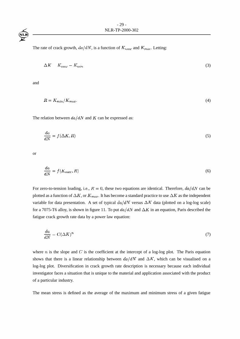
The rate of crack growth,G KH G � , is a function of
7 OQP(Rand
7 O\V � . Letting:
Z 7 s 7 O[P�R � 7 O[V � (3)
and
B s 7 O\V � H 7 OQP(R w (4)
The relation betweenG �H G � and
7can be expressed as:
G G � s � c Z 7 � B d (5)
or
G G � s � c 7 OQP(R � B d (6)
For zero-to-tension loading, i.e.,B s��
, these two equations are identical. Therefore,G KH G � can be
plotted as a function ofZ 7
, or7 O[P(R
. It has become a standard practice to useZ 7
as the independent
variable for data presentation. A set of typicalG KH G � versus
Z 7data (plotted on a log-log scale)
for a 7075-T6 alloy, is shown in figure 11. To putG KH G � and
Z 7in an equation, Paris described the
fatigue crack growth rate data by a power law equation:
G G � s m;c Z 7 d � (7)
where � is the slope andm
is the coefficient at the intercept of a log-log plot. The Paris equation
shows that there is a linear relationship betweenG �H G � and
Z 7, which can be visualised on a
log-log plot. Diversification in crack growth rate description is necessary because each individual
investigator faces a situation that is unique to the material and application associated with the product
of a particular industry.
The mean stress is defined as the average of the maximum and minimum stress of a given fatigue

- 30 -NLR-TP-2000-302
Fig. 11 Fatigue crack growth rate data
cycle. When two tests at different mean stress levels are conducted (e.g., they have the sameZ C
but
differentB
ratios) the cyclic crack growth rates will not be the same. Referring to the fractograph
of figure 10, the striation band corresponding to the cycle of lower mean stress is narrower than the
striation band for the cycle that has a higher mean stress level. This means that the fatigue crack growth
rate for the former is lower than for the latter. This phenomenon is called the mean stress effect, or
stress ratio (B
-ratio) effect. Using Paris’ equation (equation 7), one can only plot aG �H G � curve for
a givenB
-ratio. Eventually a series of equations is needed to fully describe theG �H G � behaviour
for a wide range of stress ratios. This means that different pairs ofm
and � values are needed for
each equation (for a particular stress ratio). This type of data presentation is called correlating the
data individually, because each set of data points corresponds to a certain value ofB
. (See figure 11)
In addition to the mean stress effect, there is another element that is inherently associated with theG �H G � data and needs to described. In general, aG �H G � curve appears to have three regions. The
first region is a slow-growing region (the so-called threshold), the second region is a linear region (the
middle section of the curve, described by Paris), and the third region is a fast-growing region (towards
the end of the curve whereZ 7
approaches the critical fracture toughness,7 < ). A smooth connection
of all three regions forms a sigmoidal curve representative of the entireG �H G � versus
Z 7curve for

- 31 -NLR-TP-2000-302
a givenB
. Figure 12 shows a simplified crack growth curve. Although some alloys may not exhibit a
clearly defined threshold, i.e., the entire da/dN curve is apparently linear up to the termination point,
the existence of these regions has been well recognized.
Log
da/
dN
da/dN = C( )n
n
1
-2
10-6
10
10
-4
∆Κ
Region III:- rapid, unstable crack growth
Region II:
∆Log K
- power-law region
asymptote
K or K final failure
Icc
Threshold
- slow crack growthRegion I:
Threshhold Kth∆
Fig. 12 Multiple region fatigue crack growth rate curve
The physical significance of the slow-growing and terminal (critical) region is that there are two
obvious limits ofZ 7
in aG KH G � curve. The lower limit (the threshold value
Z 7 :��) implies that
cracks will not grow ifZ 7
is smaller thanZ 7 :��
i.e.,G KH G ��� 0 when (
Z 7-Z 7 :��
) � 0. IfZ 7
becomes too high, implying that7 O[P�R
exceeds the fracture toughness7 < , static failure will follow
immediately. This is equivalent toZ 7
exceedingc f � B d 7 < i.e.,
G KH G ����� when c f � B d 7 < �Z 7 �� 0. With these additions added to the Paris’ equation (equation 7), a sigmoidal relation on a
log-log plot with two vertical asymptotes will be obtained as:
G G � s m;c Z 7 d � Z 7 � Z 7 :��c f � B d 7 < � Z 7 (8)
The valuesm
and � are respectively the intercept and slope of the line that fits through the linear
region of theG KH G � curve. The ( f � B ) term in equation 8 is pure for providing the termination point
of theG KH G � curve. It does not form any connection between
G �H G � at differentB
-ratios. Therefore
equation 8 can only be used for correlating the data individually (i.e., with oneB
-ratio at a time).
Two problems in describing crack growth rate data are faced. The first is establishing a relationship
- 32 -NLR-TP-2000-302
between all the stress ratio’s in obtaining a mathematical function that translates all theG �H G � data
points into a common scale. The advantage of this translation is that only one pair ofm
and � values
is needed for the entire data set. This approach is called correlating the data collectively. The second
problem is the need to select a curve-fitting equation capable of fitting through all three regions of
the da/dN data. Among the many crack growth rate equations published in the literature, some deal
with the mathematical formulation of a sigmoidal curve, or normalizing the stress ratio effect, or
both. Some even divide theG �H G � curve into multiple segments, attempting to obtain a closer fit
between experimental data and a set of equations. [Ref. 2 ] The next section will discuss in what
way these problems are dealt with by using different crack growth relations, based on collective data
presentation.
4.6.2 Crack growth relations for collective data presentation
At NLR the program CRAGRO, which is a modification of NASA’s NASGRO 3.00, is used for crack
growth calculations. This program is based on fracture mechanics principles and is used to calculate
stress intensity factors, to compute critical crack sizes, or to conduct safe-life analyses. For this
program an advanced crack growth relation was developed to present data collectively.
Crack growth relation
The crack growth rate calculations the program uses were developed by Forman, Newman at NASA,
De Koning at NLR and Hendriksen at ESA. This equation (equation 9) describes the behaviour of the
three regions of crack growth similar as equation 8, but differs slightly because this equation presents
the data collectively. [Ref. 8 ]
G G � s m;c Z 7 d � c f � � d �c f � B d � � f ����������������� f � ���� *"����� ��� ��� (9)
The equation uses constantsm
, � ,�
, and which must be empirically derived. The�
in the equation
is the crack opening function for plasticity-induced crack closure defined by Newman. [Ref. 9 ]
� s 7¢¡ � �£�7 O[P(R s¥¤¦ § �^_$ ] �����©¨ B � ) � } ) * B } ) , B , } ) . B .Nªif
B¬« �K) �\} )+* Bif � �A® B¬¯ �Kw (10)

- 33 -NLR-TP-2000-302
The coefficients used by equation 10 are given by;
) � s ¨ �Kw±°���² � �Kw i�³ TE} �Kw´�b² T , ª �Jµ6¶b·Q��¸ ,�¹jº&»"¼½N¾ ���/¿À)+* s c �Kw ³`f ² � �Kw´��Á f T�d ¹hº&»"¼½N¾)/, s f � ) �n� )+* � )-.)/, s � ) �n� )�* � f(11)
In these equations, T is the plain stress/strain constraint factor, andC OQP(R H S � is the maximum applied
stress to the flow stress. Both T andC O[P(R H S � are dependent on the used material.
It was shown that the lower asymptote was formulated by the threshold stress intensity factor (Z 7 :��
).
The threshold stress intensity factor is approximated as a function of the stress ratio (B
), the threshold
stress intensity factor atB sv�
(Z 7 � ), the crack length , and the intrinsic crack length ( �� ):
Z 7 :�� s Z 7 �à³��Ä(Å�Æ c f � B d£Ç�È p}É�� (12)
The appliedZ 7
appears to differ from the actualZ 7
which acts on a stress cycle. This difference
may vary for differentB
-ratios. In order to account for the mean stress effect onG �H G � , a method
to estimate the effective level of applied7
for a givenB
-ratio must be developed. The method that
accounts for this effect is known as the concept of crack closure. It has been developed for a relation
between the effectiveZ 7
andB
.
EffectiveZ 7
The concept of crack closure assumes that material near the crack tip is plastically deformed during
the fatigue crack propagation. Releasing the pressure (during unloading of a fatigue cycle), some
contact will occur between the faces of the crack surfaces due to elastically deformed material in the
surroundings of the crack tip. If the component is loaded in the following fatigue cycle, the faces of
the crack will not open immediately, but remain closed for some time during that cycle. While the
crack remains closed it is impossible to grow; crack growth is only possible during the ascending part
of the stress cycle. The net effect of closure is to reduce the apparentZ 7
to an effective levelZ 7 �zÊËÊ .
Z 7 �ÌÊËÊ s 7 O[P(R � 7 ¡ � �£� (13)
The stress intensity factor7 ¡ � �|� in this equation is the minimum stress intensity level of that cycle to

- 34 -NLR-TP-2000-302
re-open the crack, which is usually higher than the7 O[V � .
7 ¡ � �|� is dependent on material thickness,B-ratio,
7 OQP(Rlevel, crack length, and environment. Using the concept of crack closure, Elber defined
the effective stress intensity as follows:
Z 7 �ÌÊËÊ s F � Z 7 (14)
[Ref. 2, 8 ]
whereF
is defined as:
F s 7 OQP(R � 7 ¡ � �£�7 O[P�R � 7 O[V � s f � 7 ¡ � �|�7 OQP(Rf � 7 O[V �7 OQP(R s f � �f � B (15)
With these last two equations, it is possible to rewrite equation 9 into the following equation:
G G � s m;c Z 7 �zÊhÊ d �  f � ��� ���"Í?Î(Î��� Í?Î(Î Ç �� f � ��� Í?Î(Î� *"� Ê � ��� ��� (16)
whereZ 7 :�� Í?Î(Î is defined as:
Z 7 :�� Í?Î(Î s f � �f � B Z 7 �  ³� Ä(Å�Æ c f � B d Ç�È +}É � (17)
The obtained crack growth equation (16) will be used to fit reported crack growth rate data. The main
reason for presenting crack growth data7 �ÌÊËÊ versus
G �H G � is that the data can be written without the
dependency ofB
, implying that only one set of constants in equation (16) can describe the behaviour
of crack growth for different values ofB
. (See figure 13)
4.7 Finite element method to determine the stress intensity factor
Analytical solutions to problems in the mechanics of fracture are limited to idealised situations wherein:� the domain is considered to be infinite,� the material is homogeneous, and� the boundary conditions are kept relatively simple.

- 35 -NLR-TP-2000-302
Fig. 13 Individual (left) and collective (right) data presentation
To deal with practical problems of mechanics of fracture in cracked structures of finite size, arbitrary
shape, complicated boundary conditions, and arbitrary material properties, numerical methods as finite
element methods (FEM) are necessary to produce actual stress intensity factor solutions.
Using the concepts of linear fracture mechanics to predict the strength and life of cracked structures,
knowledge of the crack tip stress intensity factor as function of the applied load and geometry of the
structure is necessary. Usually, standard models with standard stress intensity factor solutions are
used to determine the stress intensity factor solution. In case of the�b���
-stage fan disc a standard crack
growth case could not be used because of the complicated geometry and a combination of multiple
load cases. To determine the stress intensity factor as a function of the geometry, a finite element
model will be used. The application of the finite element method allows analysis of complicated
engineering geometries in two dimensional, and even three dimensional problems. The basic concept
of the finite element method is that the structure can be considered to be an assemblage of individual
elements. This is done by replacing the geometry of a structure by a finite amount of elements of
finite size, which are connected through their nodal points. Known forces acting on these elements
are transmitted through the nodal points, the displacements of the nodal points are the unknowns. In
case of plane stress only two displacements, � and ! , are used. These displacements are described
with functions, e.g. assumed to vary linearly, or parabolically over the element.
In determining the stress intensity factor with finite elements, two different methods are available.
The first, direct method, determines the SIF from the stress- or displacement field near the crack.
The second, indirect method, determines the SIF through its relation with other quantities such as the
compliance, the elastic energy, or the4
integral.

- 36 -NLR-TP-2000-302
In this case the direct method will be used to define the stress intensity factor. For fracture mode I, the
stress and displacement distribution are given by :
S V´Ï s 7¢Ð8 � � � � VÑÏ crÒ d� V s m 7¢Ð 8 � � V crÒ d (18)
7¢Ðcan be calculated from the stresses and the displacements respectively:
7¢Ð s S V´Ï 8 � � �� VÑÏ7¢Ð s � Vm 8 � � V crÒ d (19)
Because finite element methods are usually formulated with displacements as the primary variables,
displacements are computed more accurately than stresses, so better results are obtained using the
lower equation of equation 19. [Ref. 10 ]
2 a
r
FEM analysis
theoretical
σ οο
σοοI
ar
oo
Kaσ
Fig. 14 FE and theoretical calculation of the SIF-solution for an infinite loaded plate with centralcrack
This last set of equations is valid in the immediate vicinity of the crack. The finite element method
calculates the stress- and displacement distribution of the model. Using the stress and displacement of
an element near the crack tip, obtained with FEM, values of7xÐ
can be obtained by using the equation
set 19. The stress intensity factor can be determined by extrapolating the constant slope, of a plotted7 H S�Ó 8 versus the distance � from the crack tip, back to the crack tip ( � sÔ�). This is graphically
shown in figure 14. [Ref. 11 ]
The reason that a difference exists between the theoretical (collocation techniques) curve and the FEM
defined curve is that for this figure normal elements are used which do not take the effects of the stress
singularity into account. Determining the7 Ð
for several elements near the crack tip, a series of val-

- 37 -NLR-TP-2000-302
ues for7ÕÐ
are obtained. Using smaller elements will produce a more accurate solution, thus very
small elements are needed. Even when using small elements, the determination of the SIF at very
small distances from the crack tip is a little inaccurate due to the inability of the elements to repre-
sent the stress singularity at the crack tip. Accounting for the stress singularity is shown in appendix
D. This appendix shows a derivation for an element which takes the effect of the stress singularity
into account, which results in more accurate SIF solutions. Engineering fracture mechanics interest is
often focussed on the singularity point, where quantities like stress become (mathematically, but not
physically) infinite. Near such singularities normal, polynomial based, finite element approximations
perform badly and attempts have frequently been made here to include special functions within an
element which can model the analytically known singular function. An alternative to special func-
tions within an element (which frequently poses problems of enforcing continuity requirements with
adjacent, standard elements) lies in the use of special mapping techniques.
14a
a
b
b14
Fig. 15 Six node triangular finite crack tip element
An element of this kind was introduced by a simple shift of the mid-side nodes of quadrilateral,
isoparametric elements to the quarter points. Although good results were achieved with such elements,
the singularity is not well modelled on lines other than element edges. Better results are obtained by
using triangular second-order elements for this purpose. (See figure 15) [Ref. 7, 11, 12, 13 ]

- 38 -NLR-TP-2000-302
5 Research prior to life time calculation
To determine the propagation life of the� ���
-stage fan disc, several aspects must be investigated.
This includes the investigation of the load spectrum, the crack growth material properties, the stress
intensity factor solution, and the stop criterion for the crack growth analysis.
5.1 Determination of the load spectrum
The life the aircraft components have is highly dependent on the weight of the missions. The initial
mission usage (or design load) specification is very important for the success and use of the aircraft.
If however, the actual mission usage of the engine deviates from the original concept, the risk of
unacceptable failures increases. This brief introduction is given to emphisize the importance of engine
load determination. Therefore loads acting on the rotating parts are to be recognised and determined.
These loads consume life of the rotating parts, and must be accounted for in the life assessment. The
most important loads on the rotating parts are:
- stresses due to bending moments, such as those due to the lift on the cascade airfoils or pressure
differences across discs,
- torsional stresses are inevitable when power is transferred by shaft torque from turbines to
compressors, and
- centrifugal forces are induced due to high rotational speeds.
The compressor fan disc is thus subjected to various types of loadings. As the air is propelled back-
wards, the compressor rotor blades tend to bend forward due to the resultant force acting on the blades.
When this force is decomposed in axial and tangential direction, the axial force tends to pull the rotor
blades in flight direction parallel to the longitudinal axis of the gas turbine shaft, and the tangential
force causes a torsional moment in the LP shaft. Another load on the compressor blades is the radial
force due to the high rotational speeds. The rotational speeds rise up to 14000 rpm, through which
high centrifugal forces are inhibited. The radial forces have no influence on the crack growth analysis
in the hub, because the forces on the rotor blades are balanced with the centrifugal force of the blades
on the opposite side.
The axial forces can not be neglected because due the distance of the forces to the hub, a bending
moment and an axial tension stress is introduced in the hub of the disc. This bending moment in
the hub is believed to cause no stresses at all, due to the high torsion stiffness of the bore. Thus the
stresses in the hub are the consequence of the axial force and the torsional moment.

- 39 -NLR-TP-2000-302
5.1.1 Stresses due to axial force
Cracks are found during inspection intervals to develop from the air/thrust balance holes. If a cracked
component is found the crack length will be reported, and the component will be rejected and replaced.
It is believed at NLR that cracks grow under an angle of 45 Ö with respect to the longitudinal axis of
the gas turbine shaft, growing to the rear of the engine. Assuming this, the stresses due to the axial
force must be much lower than the stresses due to torsional forces.
resultant
Cax
p pFax
R3R1
Cax
Fax
inlet
34 5
6
2
exit
inlet exit
resultant
1
R2
CL
Fig. 16 Impulse balance
To confirm this assumption an impulse balance over the compressor (fan) is taken (see figure 16).
The net axial force exerted on the fluid by each component is given by the streamwise increase in the
quantity;
y s×� ) }ÉY�Ø , ) (20)
This equation is usually called the impulse function in one-dimensional gas dynamics. The streamwise
axial force exerted by the internal solid surfaces of the component upon the fluid is y � RNV : > ¡ : ¡ >zÙ �y V ��ÚÛ� : > ¡ : ¡ >zÙ where]
denotes the rotor number, while the axial reaction force is equal in magnitude, but
opposite in direction. The net axial force includes all contributions of pressure and vicious stresses on

- 40 -NLR-TP-2000-302
flow path walls and any bodies immersed in the stream.
o P�R s y � RNV : > ¡ : ¡ >£Ù�� y V ��Ú±� : > ¡ : ¡ >zÙs ¨ � ,6)-, }ÉY , m ,P�RhÜ )-, ª � ¨ � *()�* }ÉY * m ,P(R ¿)�* ª} ¨ � 5 ) 5 }ÉY 5 m 5P�RËÝ ) 5 ª � ¨ � .6)-. }ÉY . m 5P(RËÞ )-. ª} ¨ ��ß ) ß }ÉY ß m ßP�RËà ) ß ª � ¨ ��á ) á }ÉY á m ßP(Rhâ ) á ª (21)
The impulse function reveals the distribution of the major forces throughout the engine, but unfortu-
nately does not precisely locate the distribution within the components. In case of a compressor or a
turbine, forces can be moved from the rotor to the stator by means of static pressure forces applied
to their extensions outside the flow path. These static pressure forces are often applied to circular
discs and are therefore known as “balance piston” loads. (This explains the need of the thrust balance
holes in the hub of the� ���
-stage fan disc.) A strategy which is frequently employed is to manage
the balance piston loads in such a way that most of the axial force is delivered to the stators, which
are firmly attached to the outside casing of the gas turbine. This leaves only enough axial force on
the shaft, which is attached to the rotors, to guarantee that the shaft thrust bearings, which prevents
the axial motion of the shaft, always feels enough force to prevent the bearings from skidding, which
rapidly consumes their life. This implies that the force exerted by the rotor is smaller than the value
calculated with the impulse balance. [Ref. 14]
Solving the impulse function requires knowledge of many parameters as the inlet and outlet velocities
(which are dependent on the angle of incidence), the static pressures at the inlet and outlet and the
accompanying densities, and the geometry of the compressor disc and rotor blades. Many of these
parameters are unknown. These parameters can be determined with extensive research, but that is
beyond the scope of this project. To quantify the net axial force, an estimation will be made using the
geometry of the compressor blade. The angle of the blade is observed to vary between 55 Ö at the root
of the blade, to an angle of 35 Ö at the tip of the blade. The blade angle at mid-size is therefore 45 Ö .
The assumption is made that the resultant axial force seizes at this point. With the known acting torque
and the blade angle, the net axial force can be calculated to be equivalent to the tangential force (the
tangential force is defined as the torque divided by the radius to the mid span). The obtained force is a
conservative value, because the resultant force seizes at a distance larger than 50% of the blade height
(usually approximately 70%), where the tangential force is smaller due to the increase in radius, and

- 41 -NLR-TP-2000-302
the blade angle is less than 45 Ö . [Ref. 15]
S s o : P �) �Nãhäs f � � f � . H �Kw i ²¸ 5 c f�f6³ w±å�° , � f ���Kw´�b° , d s fËi w±æ 2 � (22)
The steady state torque load at the design point is 12 ç �E� , resulting in a mean shear stress of 88.52 � . The magnitude of the axial stress is f ²bè of the value of the shear stress. The effect on the
orientation in which the crack grows can be calculated with equation B.6 of appendix B. In appendix
B the derivation of stresses to the principal stresses is shown.
Inserting S R s fËi w±æ 2 � , S a sé� 2 � , and W RNa sé°�°�w±² 2 � in equation B.6 of appendix B shows
that the influence of the axial force on the direction of the crack is observed to be minor. Due to
the axial load the crack direction will be 42.8 Ö with respect to the longitudinal axis in stead of 45 Ö .
To determine the influence of this change in growth direction due to the axial load, the life time is
calculated (with use of CRAGRO) for two bi-axially loaded infinite plates. One of the plates is loaded
with a S * which is equal, but with reversed sign, to S , . The other plate is loaded with a S * which is
-0.857 times S , . The first plate is subjected to a maximum/minimum load of respectively 88.5 2 � and -88.5 2 � , while the second plate is subjected to a maximum/minimum load of respectively
95.57 2 � and -81.95 2 � . (These loads are determined by filling in equation B.7 of appendix
B) Figure 17 shows the stress intensity factor solutions for both the load cases. This figure shows
that the SIF solution of the case with the axial load is smaller than the case without the axial load. A
conclusion which could easily be drawn from this figure is that the life-time of the axially loaded plate
is bigger than the normally loaded plate, because the SIF appears to be smaller. This is in fact not true,
because the vertical axis is scaled to the net stress. The stresses the axially loaded plate experiences
are higher, resulting in a life time less than the case where the axial load is neglected. Two runs in
CRAGRO are made. The result of the axially loaded plate is 88910 cycles for a crack to grow to 4.5��� . For the other crack case, without the axial stress, a lifetime of 105010 cycles is obtained. The
results of the life time calculations for these biaxially loaded infinite plates show that neglecting the
axial component in the load spectrum results in an overestimation of approximately f °bè from the
plate where the axial force is not neglected. As noted earlier, a conservative approach is used, the
actual percentage might be less.
This percentage is higher than anticipated in the first place, where the effect of the axial stress was
neglected. The axial force is omitted in further calculations, but may produce a significant effect in
the life time calculation. Therefore for further calculations the angle of crack growth is assumed to be

- 42 -NLR-TP-2000-302
45 Ö . [Ref. 14, 15]
0
1
2
3
4
5
6
0 1 2 3 4 5 6 7 8 9 10
crack length [mm]
KI/S
nom
Without Fax With Fax
Fig. 17 SIF solution of two load cases
5.1.2 Stresses due to torsional effects
In the past years, NLR has build up expertise on gas turbine engine performance by supporting both
military and civil aircraft operators as well as manufacturers with projects related to engine perfor-
mance and handling, diagnostics, fuel consumption, health monitoring, etc. As an aid to predict,
describe or analyse gas turbine behaviour, advanced modeling tools have been developed. NLR’s
main tool for gas turbine engine performance analysis is the Gas turbine Simulation Program (GSP).
This program enables both steady-state and transient simulations of selected gas turbine configura-
tions. An accurate model of the F-16 Pratt & Whitney gas turbine has been made at NLR, which will
be used to determine the stresses in the compressor disc hub. To determine the stress in the disc due
to torsion, the flight conditions and some engine parameters must be known. A system that measures
the flight conditions and engine parameters several times per second is installed in the aircraft. The
data is gathered by an acquisition system, called FACE, which is partly developed at NLR. This data
acquisition system records for instance altitude, speed, free air temperature, rotational shaft speeds,
turbine inlet temperature, exhaust nozzle area, and the fuel flows of the primary and core/duct aug-
mentor (and many more if necessary). The data are imported in an Excel worksheet to be processed
into a format usable for GSP. The variety in output data generated by GSP is wide, but for the load
spectrum of the fan disc the torsional load on the fan shaft is needed. Fortunately all medium induced
forces of the three sets of compressor blades will be transmitted through the�b���
-stage fan disc. The� ���-stage fan disc transmits all loads of all three fan discs to the low pressure shaft through the hub.

- 43 -NLR-TP-2000-302
The chosen torsional moment is not usable for crack growth programs, and must therefore be trans-
lated into (shear) stresses to be implemented in the load sequence. When a torque is applied to a
uniform member with a circular cross section it tends to twist the member by rotating through an
angleU
(angle of twist). During the twist all cross sections remain plain and undistorted (only for
circular cross sections). The angle of twist is described by:
W � s D 4 s 3 U(23)
The polar moment of inertia is described for a hollow shaft with inner diameter0 *
and outer diameter0 ,by:
4 s �i � c 0 5, � 0 5 * d (24)
To obtain a relation between the torque, the radii, and the shear stresses, equation 24 is substituted
in equation 23. The shear stresses are proportional to the distance from the centerline, resulting in a
maximum shear stress in the outer most fibre of the loaded member. (The geometry data of the hub is
listed in table 2) (Figure 18 shows the shear stress distribution in a hollow shaft.)
W , s 0 , D¸* ß ¨ 0 5, � 0 5 * ª sêÁ_w±°�æ ³ æ � f � � ß � D (25)
τ
Shaft
min
[MPa]
[mm]ρ
Torque
τ
maxτ
Fig. 18 Front view of a shear stress distribution in a torque loaded hollow shaft
This equation will be used to transform the torques, obtained with GSP, into shear stresses.
To calculate the torques, a GSP model of the Pratt & Whitney PW-F100-220 has been made at the
helicopter department. With the data recorded by the FACE system as input parameters, the torque
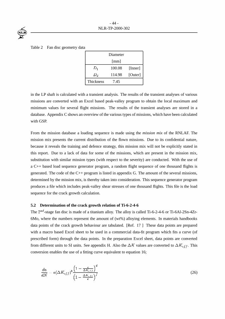
- 44 -NLR-TP-2000-302
Table 2 Fan disc geometry data
Diameter
[mm]0 *100.08 [Inner]0 ,114.98 [Outer]
Thickness 7.45
in the LP shaft is calculated with a transient analysis. The results of the transient analyses of various
missions are converted with an Excel based peak-valley program to obtain the local maximum and
minimum values for several flight missions. The results of the transient analyses are stored in a
database. Appendix C shows an overview of the various types of missions, which have been calculated
with GSP.
From the mission database a loading sequence is made using the mission mix of the RNLAF. The
mission mix presents the current distribution of the flown missions. Due to its confidential nature,
because it reveals the training and defence strategy, this mission mix will not be explicitly stated in
this report. Due to a lack of data for some of the missions, which are present in the mission mix,
substitution with similar mission types (with respect to the severity) are conducted. With the use of
a C++ based load sequence generator program, a random flight sequence of one thousand flights is
generated. The code of the C++ program is listed in appendix G. The amount of the several missions,
determined by the mission mix, is thereby taken into consideration. This sequence generator program
produces a file which includes peak-valley shear stresses of one thousand flights. This file is the load
sequence for the crack growth calculation.
5.2 Determination of the crack growth relation of Ti-6-2-4-6
The� ���
-stage fan disc is made of a titanium alloy. The alloy is called Ti-6-2-4-6 or Ti-6Al-2Sn-4Zr-
6Mo, where the numbers represent the amount of (wt%) alloying elements. In materials handbooks
data points of the crack growth behaviour are tabulated. [Ref. 17 ] These data points are prepared
with a macro based Excel sheet to be used in a commercial data-fit program which fits a curve (of
prescribed form) through the data points. In the preparation Excel sheet, data points are converted
from different units to SI units. See appendix H. Also theZ 7
values are converted toZ 7 �zÊËÊ . This
conversion enables the use of a fitting curve equivalent to equation 16;
G G � s c Z 7 �ÌÊËÊ d ä � f � <��� Í?Î(Î � �� f � ��� Í?Î(Î� � Ê (26)

- 45 -NLR-TP-2000-302
where, s m� s �I s Z 7 :�� Í?Î(ÎG s �M s c f � � d 7 <� s A difficulty in determining the fit parameters arises. The fit parameters I and M are assumed to be
constant. In fact these fit parameters are not constant, but are dependent on the stress ratioB
. Due to
this dependence a loop (iteration) within the fit process is needed. (Because not all data points have the
same stress ratio.) This loop and the small amount of datapoints make the fit process quite complex
and thus instable, so no solutions are found for the fit parameters. For this reason fit parameters I andM are assumed to be constant, resulting in a marginal error in the fit solution.
However, the main difficulty in the fitting process is the absence of data points in the neighbourhood
of the threshold value and the critical value. Therefore, often no convergence takes place in the fit
proces solution procedure, or big inaccuracies occur. Due to the divergence, the threshold and critical
value could not be obtained, and therefore values from the literature are used. Although the exact
value is not known, the threshold is seen in the materials database of NASGRO to be of the same
magnitude for various titanium alloys (a relatively small value is chosen to obtain a conservative
calculation). The value of7ÕÐ < on the other hand is not the same for most titanium alloys.
7�Р< is the
plain strain fracture toughness, which is a measure for the maximum crack resistance of a material.
Due to the small diameter to thickness ratio in our case, the state of stress is plane stress. This means
that deformations can easily occur and in that case the stress intensity factor depends on the plate
thickness. The critical fracture toughness is dependent on the thickness of the specimen, and tends
to increase for decreasing thickness. See figure 19. [Ref. 2, 7 ] This means that the7 < (the plain
stress fracture toughness) is slightly higher than the7�Р< value. In this case the actual
7xÐ < from the
materials handbook will be used. Because of the use of this value, crack growth calculations will be
cut off sooner than expected, which implies that a conservative life time will be obtained. For the
threshold value as in equation 17, theZ 7 � = 69.5 2 � 8 ��� , which will be used. The
Z 7 � in
this equation is theZ 7
atB së�
. For the plain strain fracture toughness an average value of 13402 � 8 ��� is used. [Ref. 17 ]
Because of these difficulties, two more methods are used to fit the data points. This is done with a
simplified fit curve, which does not deal with the threshold and critical values. The simplified fit curve

- 46 -NLR-TP-2000-302
Thickness
Kc
KIc
Fig. 19 The thickness effect on7 <
has the following form:
G G � s c Z 7 �ÌÊËÊ d ä (27)
where,
as
C
bs
n
This equation is used for both the commercial fit program as the trendline function within Excel.
Figure 20 shows a fit of the Paris equation (equation 7) of the reported data points from ref. [Ref.
17 ] The fit parameters obtained with the three fit methods are tabulated in table 3. Table 3 shows
Table 3 Fit parameter overview of different fitting processes
Fit parameter Method I Method II Method III
Fit program Fit program Excel trendline
a C f w i ²�æ�å�æ � f � ��* � ��w±° f �bå � f � ��*"* Á � f � ��*"*b n
��w i �bæ�²bÁ 2.5603649 2.4166
cZ 7 :�� Í?Î(Î � ��w±æ�°�� i å � f � � á
d pæ�w´���bæ�� � f � �9.
ec f � � d 7 < f � i æ�w´� f æ
f q²�w i ° i�³�i � f � �9,

- 47 -NLR-TP-2000-302
that the various fit processes produce slightly different fit parameters. To describe the materials crack
growth curve,m
and � from all the three methods are taken from table 3, the7 Ð < is taken from
reference [Ref. 17 ], and the threshold value is taken from the NASGRO materials database (see page
45), which are to be used in the crack growth program.
0.00001
0.0001
0.001
100 1000∆∆ Keff [MPa sqrt(mm)]
da/d
N [
mm
/cyc
le]
Test data
Power (Test data)
Fig. 20 Fitted crack growth data points
5.3 Determination of the SIF solution
To determine the stress intensity factor solution of the� ���
-stage compressor fan disc, a finite element
model is needed, because the geometry of the fan disc is too complex to use standard (infinite plate)
SIF solutions. The fan disc is cyclic symmetric, and has 21 drilled air/thrust balance holes. The
function of the air/thrust balance holes is to balance the pressure between the front and back side of
the fan disc. [Ref. 17 ] Using the cyclic symmetric property in the FE model, only a small part (*ì :�� )
of the complete fan disc has to be modeled. Cracks are assumed to grow from the air/thrust balance
holes under a 45 Ö angle with respect to the axial direction, and will grow in the hub of the�b���
-stage
compressor fan disc. These cracks are considered through the thickness cracks so that the model
can be constructed of two dimensional shell elements. For simplification reasons the whole model is
constructed with the same shell thickness, because the hub has approximately the same thickness in

- 48 -NLR-TP-2000-302
various sections. In the model the spacer/holder is not modeled, which will result in a conservative
answer, because the crack growth rate will decrease due to the thicker section of the spacer/holder.
The hub is connected to the disc, which is constructed of a relatively large piece of material called
the bore, so that the model of the hub will be assumed to be supported. The boundary conditions are
: �&í së� �`�&î sï� �`� {�q � së� �`� {�qKð�së� �`� {�q ' sï�. On the opposite side the load is applied at the
middle of the spline as a distributed load on the shell elements. A graphical image of a FE model is
shown in figure 21. This model is made for the stress intensity factor solution calculation of a 6 ���crack in the direction of the spline.
XY ZXY Z
Fig. 21 Finite element model
Modeling the crack in the structure requires knowledge of the coordinates of the crack tip center
on the surface. For that reason an Excel based program is written which calculates the coordinates
as well as the length of the crack with respect to the origin of the crack. This is an important tool
for constructing and meshing the model in a FEM program. The SIF solution is calculated with the
use of PATRAN/NASTRAN. PATRAN is the pre- and post processor, which is used to create the
geometry and the mesh. In the mesh at the cracktip in the surface of a square millimeter surrounding
the cracktip, 4 elements are deleted. Of this model a data deck is generated for NASTRAN, the
calculation program. Before running the data deck with NASTRAN, the data deck file is altered to

- 49 -NLR-TP-2000-302
fit a special cracktip element in the mesh where the 4 elements have been deleted, because PATRAN
does not support cracktip elements. This special NASTRAN cracktip element is called a CRAC2D
element. Appendix I describes the use of this special crack tip element.
Figure 22 shows the deformed model, while figure 23 shows the first principal stress in the model.
XY ZXY Z
Fig. 22 Deformed finite element model
Several SIF solution calculations are performed for different crack sizes. These calculation are per-
formed for a crack in the direction of the support and for a crack in the direction of the spline. The
results of these calculations are graphically displayed in figure F.1 and figure F.2 of appendix F. Fig-
ure F.1 shows the results of the calculations compared to the results for a bi-axially loaded infinite
plate with one hole. Figure F.2 shows even more stress intensity factor solutions for different loading
types. Explanation of the legend is given in appendix F.
The figures clearly show that for large crack sizes, the SIF solution of the compressor fan disc ap-
proaches the solution of a bi-axially loaded infinite plate with a hole. For small crack sizes the in-
fluence of the thrust balance holes and the support is that large that the actual fan disc SIF solution
deviates from the infinite solution. The actual SIF solution of the compressor fan disc will closely
follow the path of the FEM calculated SIF solution, but will deviate when the crack approaches the

- 50 -NLR-TP-2000-302
XY Z
1.07+03
9.96+02
9.19+02
8.42+02
7.64+02
6.87+02
6.10+02
5.32+02
4.55+02
3.78+02
3.01+02
2.23+02
1.46+02
6.85+01
-8.78+00
-8.61+01XY Z
Fig. 23 Maximum principle stress in finite element model
length of approximately 4.5 ��� due to the increase in thickness of the spacer/holder, which was not
modeled.
5.4 Stop criteria for crack growth calculation
Failure or rejection of a component that contains a crack due to crack extension can be the result of
three different causes.
- failure due to exceeding the plain strain fracture toughness7�Р< ,
- failure due to exceeding the net yield stress, or
- rejection due to technical or environmental issues (e.g. large cracks in fuel tanks will cause
spilling of fuel, and therefore unacceptable)
Which one of the three stop criteria is applicable in case of the compressor fan disc calculation must
be investigated prior to performing the crack growth calculation.

- 51 -NLR-TP-2000-302
5.4.1 Exceeding the fracture toughness
From the load spectrum database the highestZ W (shear stress) can be obtained. This is observed to
be approximately 116 2 � . With the use of the stress intensity factor solution theZ 7
(max) can
be calculated. From the figures F.1, and F.2 one could imagine that the component will fail at the
highest SIF. The local maximum SIF is reached at a crack length of 1.4 ��� with a value of²�w±æ�°
.
This corresponds with aZ 7
of 660 2 � 8 ��� . The plain strain fracture toughness is assumed to
be 1340 2 � 8 ��� , which is higher than the local stress intensity factor, so the critical crack size
is not reached at a crack length of 1.4 ��� . To obtain an indication of the critical crack length, the
biaxially loaded infinite plate with hole SIF solution and ��ñ �� ½ ¿s f�f w±²�² are used. This reveals (see
figure 24) that the critical crack length will be much larger than 1.4 ��� . The critical crack length
exceeds the distance to the spacer/holder, so that the actual crack will stop growing or its crack growth
rate will decrease. (The crack length to the spacer/holder is 5.5 ��� )
0
2
4
6
8
10
12
0 10 20 30 40 50 60 70 80 90
crack length, a [mm]
KI/
S nom
Fig. 24 Biaxially loaded infinite plate with hole

- 52 -NLR-TP-2000-302
5.4.2 Exceeding the net yield stress
To determine the critical crack size at which the yield stress will be exceeded, an approximation of the
compressor disc hub, a simple hollow cylinder, is used. The first principal stress ( S * ) tends to open
the crack to 45 Ö with respect to the axial direction. Along the surface of the cylinder an imaginary
crackc L?d can be assumed to be 8 � � � �&�&L?MN��� q � s�ò f6³`f ��� . If a certain crack length is reached the
net yield stress can be exceeded and the component will fail. This can be roughly estimated with:
S * LL&� c =� G ] _� � ¡ Ú±� d ¯ S a�V �zÚ±� (28)
S a�V �zÚ±� s f�f Á�� óõô ÅS * s f ��² óõô Å c÷ö`ø�ù Æ µ ù�ö Å�ú · Ä ø(û ·(·�ü Å ø ü ø ¶bý Ä(þ û ·�ÿ ö`ö ¶ ø Ä dFrom which it follows that the crack can grow to a length of 120 ��� before failure due to the
exceeding of the net yield stress occurs.
5.4.3 Other rejection reasons
In aircraft wing structures components are rejected when cracks have extended to such lengths that
fuel, oil, or hydraulic fluid cannot be contained in their designed compartment. In case of the hub it
might be possible for cracks to grow to such rates that the the high pressure of the inner spool leaks
to the outer spool.
5.5 Implementation
It is not likely for the crack to grow to rates specified in paragraph 5.4.1 or 5.4.2, because these values
are very large they will result in large life times. Pratt & Whitney uses critical crack sizes which are
substantially smaller than the crack sizes determined in paragraph 5.4.1 or 5.4.2, and must therefore
have found a reason to assume small critical crack sizes. Therefore standard critical crack sizes from
Pratt & Whitney are used. [Ref. 19 ]
The results of the above mentioned aspects will be used as input for the crack growth calculation
program CRAGRO which will produce a crack based propagation life time. CRAGRO is a modular,
stress intensity factor based, crack growth calculation program developed at NLR. This program is
based on the NASGRO crack growth calculation program developed by NASA, but differs because of
its modular design, which makes it relatively easy to expand the program with new equations or new
models. Both programs lack the ability to take into account the contribution of creep and the influence
of temperature. However, because the temperature in the fan disc is not very high, creep plays no role
and can therefore be omitted in the calculation.

- 53 -NLR-TP-2000-302
6 Crack growth calculation results
In the previous chapter all steps for the crack growth calculation are described. All these steps are
incorporated in the crack growth program CRAGRO. The results will be presented and discussed in
this chapter.
6.1 Results
As mentioned before the main object of this investigation is to determine whether the crack growth
calculation could be made and secondly to determine whether the propagation life time of the� ���
-
stage fan disc is plausible. The propagation life time is the time in which an initial crack grows to the
critical value. The propagation life is expressed in TAC’s, which are the Total Accumulated Cycles.
Each flight the RNLAF makes consumes a certain amount of cycles, expressed in the CCY number
(Calculated CYcles). Dividing the TAC number by the CCY number the propagation life time of the�����-stage fan disc is obtained in terms of flights. Due to the confident nature of the CCY number
(because it reveals the RNLAF defence and training strategy) it will not be explicitly stated in this
report. The CCY number seems to fluctuate over the years, because of its dependence on the type
(mission mix) and the amount of flights. [Ref. 18] Therefore the propagation life time (determined
by Pratt & Whitney Aircraft, PWA) is based on the lowest and the highest CCY number. The minimum
life time according to PWA using appropriate CCY data of the past years is 2925 flights, while the
maximum life time is 3382 flights.
The load sequence file contains 1000 flights. Because of this amount of flights, the crack growth
calculation will be cut off in the middle of the file. CRAGRO reports in which line of the load
sequence file the critical crack size or the fracture toughness is exceeded. Therefore a C++ program
is written to determine in which flight the crack growth calculation is cut off. This program is called
Mission counter. See appendix G for the code of that program.
The initial crack size used in CRAGRO is the crack size PWA uses for their calculations, the initial
crack size ( V ) is 0.254 ��� . Table 4 shows the results of crack growth calculations for the indicated
critical crack lengths, using the initial crack size. PWA assumes different critical crack sizes for
different parts of the component. The first column of table 4 shows typical values used by PWA for
various parts in compressor discs. [Ref. 19 ] None of these parts correspond with our crack case, so
that the calculated life times are not significant. The crack sizes are merely used for an indication of
actual critical crack sizes.

- 54 -NLR-TP-2000-302
Table 4 Overview of the CRAGRO results for various critical crack sizes
Critical crack size Fit method I Fit method II Fit method III
mm flights flights flights
1.6764 1062 1266 1130
2.3368 1523 1800 1602
2.7432 1822 2139 1912
2.8448 1887 2229 1993
3.1496 2124 2498 2234
4.2672 3025 3569 3195
4.7752 3467 4107 3663
4.8260 3513 4164 3711
6.2 Discussion of the results
Unfortunately the main disadvantage of the reported PWA propagation life time values is that it is not
reported whether the component fails due to reaching the critical crack size, or that the component
fails due to insufficient remaining strength, or is rejected due to another reason. Due to the unknown
failure mechanism it is unknown when the crack growth calculation is cut off. Therefore, critical crack
sizes of a f g : -stage fandisc and a�����
-stage fan disc from the first design have been used.
The propagation life times of Pratt & Whitney can not exactly be compared with the calculated life
times, due to the fact that the used critical crack sizes are not applicable for our used crack geometry.
Most of the critical crack sizes in table 4 are taken from other locations than the hub, implying different
load cases. The results however, show that the life times calculated with CRAGRO are of the same
magnitude as the PWA life times. The results are slightly higher than the PWA results, because
the effect of the axial force is not accounted for in the crack growth calculation, approximations in
determining the crack growth relation, and inaccuracies in the SIF solution exist.
The results show that the design life time of the Pratt & Whitney calculations can be approximated
assuming relatively short critical crack sizes of approximately 4.5 ��� . Therefore Pratt & Whitney
must have found a mechanism present in the component which adds to the normal loading, or Pratt
& Whitney scaled their loading schedule with a safety factor. The loading sequence Pratt & Whitney
uses to determine the propagation life of the� ���
-stage fan disc is unknown and could well be scaled
to account for problems such as augmentor instability. If the actual failure mechanism, or the severity
of the Pratt & Whitney loading sequence is known, the propagation life time of the� ���
-stage fan disc
could be determined.

- 55 -NLR-TP-2000-302
The� ���
-stage fan disc of an USAF test engine failed prematurely (well before the propagation design
limit). A confidential PWA report, [Ref. 20 ] , obtained from the RNLAF showed the premature
failure to be due to combustion instability. Combustion instability induces pressure pulsations which
produce torsional vibrations that excite the natural frequency of the disc. To determine the life of the
prematurely cracked disc the torsional vibration loading must be added to the load sequence. The
difference in propagation life time due to combustion instability in the augmentor is a result from idle
to maximum augmentation. The combustion of fuel in the augmentor fuel nozzles produce pressure
pulsations, which produce two effects. The first effect is that the pulsations are in direct contact with
the fan-blades through the bypass (fan) duct. If the magnitude of these pulsations are big in relation to
the size of the duct, all fan blades experience a change in angle of incidence, and therefore a change in
the load magnitude and load direction. The second effect is that also the turbine rotor can contact the
pressure pulsations causing the angle of incidence of the blades to alter. This effect results in torsinal
vibrations and can excite the rotor in a torsional resonant mode. This extra load spectrum, which is
not investigated, must be added to the normal loading sequence. This extra load spectrum consists of
high frequency, low amplitude loads. These loads will lead to High Cycle Fatigue (HCF). HCF is of
less importance for crack growth calculations because the life time can be expressed in minutes, so
that the life of the component is strongly dependent on when the effect occurs. [Ref.15, 16, 20 ]

- 56 -NLR-TP-2000-302
7 Conclusions and recommendations
7.1 Conclusions
- The life predictions, made by Pratt & Whitney, can be reproduced with CRAGRO, using realis-
tic assumptions for the initial and critical crack length, even when the 20% error due to the axial
compressor force is omitted in the load sequence. The path or stratagy followed is independent
on the path followed by Pratt & Whitney.
- The performed crack growth calculations for the�b���
-stage fan disc are in fact design calcula-
tions. This propagation life time is based on low cycle fatigue (LCF). If the mechanism for
fracture or the severity index (safety factor) of the load sequence is known, the crack growth
calculation indeed can be performed. This life limit differs from the actual life limit from the
fractured test stand engine, because this fan disc is subjected to high cycle fatigue (HCF).
- Actual life predictions, for other components, can be performed when accurate material data,
load sequence, stress intensity factor solution, and initial and critical crack lengths are known.
A powerful tool in the determination of the stress intensity factor solution, is the use of finite
elements. Usually infinite plate, or standard plate stress intensity factor solutions are used.
These solutions are not applicable due to the high complexity of the component. This report
shows that the two dimensional stress intensity factor solution for a real component can be
calculated using FEM techniques.
- Due to large uncertainties in the determination of the fit parameters, uncertainties in the life time
are obtained. To obtain a close fit for the crack growth calculation, many crack growth data is
necessary, especially at the threshold and at the fracture toughness to define the asymptotes.
7.2 Recommendations
- To determine the stress intensity factor solution of a cracked component, many calculations
for different crack lengths must be made. The geometry of the FE model differs slightly from
one calculation to another. The main differences are the crack size and the mesh. The pro-
cess of determining stress intensity factor calculations is time consuming, and could simply be
computerised, so that the determination of the stress intensity factor solution could be speeded
up.
- In this report the propagation design life time is determined for a component subjected to LCF.
The actual test stand engine was also subjected to HCF. To account for HCF in the calculations,
eigen frequency and computational fluid dynamic (CFD) calculations are needed. HCF life
limits usually are very short, most of the times calculated in minutes. Therefore it should
be considered if eigen frequency and CFD analyses are useful, if the excitation in the eigen
frequency occurs failure is likely to follow very quickly. This could occur in the beginning or

- 57 -NLR-TP-2000-302
at the end of the propagation life time. The actual life limit, including HCF, will be strongly
dependent on when the excitation in the eigen frequency occurs.
- Most cracks start their life as corner cracks before they grow to through the thickness cracks.
Hence a three dimensional stress intensity factor solution could be made and compared to the
two dimensional stress intensity factor solution.
- Try to discover whether PWA has scaled their load sequence or what critical crack length they
used to stop the calculation.
- Research on the extend of the axial compressor force by including the determination of the
force within GSP using the impulse balance. Because this feature will not be used by most
commercial GSP owners, the necessary data could be presented as output data, and processed
in for instance an Excel sheet.
8 Discussion
The discussed thesis is presented and defended for an exam committee. The committee approved the
thesis, but had some remarks.
FEM related remarks:
- One of the major concerns is that the FEM model is constructed as*ì :�� of the total hub, and
constrained with cyclic symmetric constrains. This simplification is not quite correct, because
this means the total hub would contain seven cracks. The effect of this representation would be
that the model is less stiff than a model of the complete hub containing only one crack. This
will yield a conservative answer. The problem with models of complete constructions is that
the calculation time is much larger than for parts of those constructions.
- The load is introduced at half the distance of the spline. The spline would not permit the hub
to rotate along the radial axis. This is not modeled, but again would this lead to a more stiff,
consevative, model.
9 References
1. Grooteman, F.P.; Fundamentals of Stochastic Analysis and Risk Assessment, National
Aerospace Laboratory NLR The Netherlands, February 1997, CR 97092 L.
2. Liu, A.F.; Structural Life Assessment Method, ASM International, first edition, 1998.
3. Cohen, H.; Gas Turbine Theory, Longman Group Limited, fourth edition, 1996.

- 58 -NLR-TP-2000-302
4. United Technologies Pratt & Whitney; F100 Fan Report, United Technologies Pratt & Whit-
ney, April 1990, FR-21278.
5. Tinga, T.; Aerospace Lifing Methods, specifically for gas turbines, National Aerospace Labo-
ratory NLR The Netherlands, November 1998, CR 98511.
6. Kolkman, H.J.; Discussion of the PWA lifing concept for the F100 engine -CIP task 463-,
National Aerospace Laboratory NLR The Netherlands, 1996, CR 96489 L.
7. Broek, D.; Elementary Engineering Fracture Mechanics, Sijthoff & Noordhoff, second edi-
tion, 1978.
8. Fatigue Crack Growth Computer Program ”NASGRO” version 3.00, National Aeronautics
and Space Administration, Lyndon B. Johnson Space Center, July 1996.
9. Newman Jr., J.C.; A Crack Opening Stress Equation for Fatigue Crack Growth, International
Journal of Fracture, March 1984, Volume 24, R131-R135.
10. Fenner, R.T.; Engineering Elasticity,Application of Numerical and Analytical Techniques,
Ellis Horwood Limited, first edition, 1986.
11. Chan, S.K.; et. al.; On The Finite Element Method in Linear Fracture Mechanics, Engineering
Fracture Mechanics, 1970, Volume 2, pp. 1-17.
12. Atluri, S.N.; Computational Methods for Plane Problems of Fracture, Elsevier Science Pub-
lishers, Volume 2, 1986.
13. Zienkiewicz, O.C.; The Finite Element Method, mcGraw-Hill, fourth edition, 1994.
14. Mattingly, J.D.; Heiser, W.H.; Daley, D.H.; Aircraft Engine Design, AIAA Education Series,
third edition, 1987.
15. Wolf, W.B. de; Verbal contact, National Aerospace Laboratory NLR The Netherlands, Jan-
uary 2000.
16. Visser, ir. W.; Verbal contact, National Aerospace Laboratory NLR The Netherlands, January
2000.
17. Damage Tolerant Design Handbook, Metals Ceramic Information Center, December 1993,
Volume 24, Chapt. 4.
18. Heida, J.H.; Slauerhoff, J.F.; (Classified), RNAF F100 Engine Usage Monitoring 1994-1997
(Confidential), National Aerospace Laboratory NLR The Netherlands, 1998, NLR-CR-99021.
19. Nethawa, D.H.; King, T.T.; F100(3) Engine Structural Durability and Damage Tolerance
Assessment Final Report, Pratt & Whitney Aircraft Group, 6 June 1980, FR-10481-9.
20. Pratt & Whitney; (Classified); Improved Durability� ���
-stage fandisk (Safety Improvement),
Pratt & Whitney, July 1996, Engineering Change Proposal (ECP) 94NA085.
21. Prof. dr. ir. L.J. Ernst; College diktaat Sterkte en Stijfheid II, Technische Universiteit Delft,
Juni 1997.
22. Henshell, R.D.; Crack Tip Finite Elements are Unnecessary, International Journal for Nume-
rical Methods in Engineering, 1975, Volume 9, pp495-pp507.

- 59 -NLR-TP-2000-302
23. Newman, J.C.; An Improved Method of Collocation for the Stress Analysis of Cracked Plates
with Various Shaped Boundaries, NASA, 1971, TN D-6376.
24. Rooke, D.P.; Cartwright, D.J.; Compendium of Stress Intensity Factors, The Hillingdon Press,
first edition, 1976.

- 60 -NLR-TP-2000-302
This page is intentionally left blank.

- 61 -NLR-TP-2000-302
Appendix A Stresses and displacements at the crack tip
Irregularities such as holes, screw threads, and notches present in a member subjected to loading,
may locally produce higher stresses than the remotely applied stress. This phenomenon is called
stress concentration. The ratio of the true maximum stress to the stress that is calculated by ordinary
formulas of mechanics using the net section (and ignore the changing in stress distribution), is the
factor of concentration. For an infinite plate with a remotely applied uniform stressC
, the theoretical
stress concentration factor for an elliptical hole of semimajor axis (on the $ -axis) and end radius Yis equal to:
7¢: s f } � � È Y (A.1)
or
7¢: s f } � � � � (A.2)
b
-a a
-b
ρ
y
x
Fig. A.1 Elliptical crack
where � is the semiminor axis (on the % -axis). (See figure A.1) In case of a circular hole, if equals� , the well-known stress concentration factor for a circular hole in an infinite sheet appears.c 7 : s i d
When � approaches zero, the ellips may be regarded as a crack. As a result the stress concentration
factor becomes infinitely high. The local stress and displacement distributions near the crack tip, with
coordinate system according to figure A.2, are given by:
S a s � ñ� , ¸ > µ6¶b·�� ,�� f } · ù Æ � ,�� ] � . �,��S R s � ñ� , ¸ > µ6¶b·�� ,�� f � · ù Æ � , � ] � . �,��W RNa s � ñ� , ¸ > · ù Æ � , µ6¶b·� , µ6¶b· . �, (A.3)

- 62 -NLR-TP-2000-302
For plane strain this becomes:
S î s X c S R } S a dW R î s W a î sé�! s ��ñ�� >, ¸ · ù Æ � , � � � � X � µ6¶b· , � , �� s � ñ�� >, ¸ µ6¶b·�� ,�� f � � X } · ù Æ , � , �# s �(A.4)
In these equations � is the absolute distance from the crack tip, ! , � , and # the displacements corre-
sponding to the directions of % , $ , and ' respectively. The constant3
is the shear modulus of elasticity
(or the modulus of rigidity), and is related to Young’s modulus and Poisson’s ratio by:
3 s 1� c f } X�d (A.5)
For plane stress it yields:
S9î s W R î s W a î s �! s ��ñ � >, ¸ · ù Æ � , � � � � ���*�� � � � µ6¶b· , � , �� s � ñ � >, ¸ µ6¶b· � ,�� f � � � �*�� � � } · ù Æ , � , �# s � � ñ î� , ¸ > � �*�� � � µ6¶b· � ,(A.6)
r
θ
Crack
y
x
τ
σy
xσ
xy
Fig. A.2 Coordinate system for stress/strain solutions

- 63 -NLR-TP-2000-302
In these equations7ÕÐ
is denoted as as the stress intensity factor, referring to the crack opening mode,
which is the most common type of fracture. It should be emphasized that7
is in no way related to
plane stress or plane strain, because in either case the crack tip stress distributions are unchanged.
The difference between the hypothetical plane stress and plane strain loci is not due to the stress
components in the plane, because they are identical. Referring to A.3,7 Ð
is not a function of the
body, including the crack, i.e., crack size, geometry, location of the crack, and loading condition. The
difference between plane stress and plane strain is hinged on the presence or absence of transverse
constraint in material deformation in the vicinity of the crack tip.
In equations A.3, A.4, and A.6 some higher-order non-singular terms have been omitted. If � becomes
rather small compared to planar dimensions, the magnitudes of the non-singular terms become negli-
gible compared to the leading f H 8 � term. Therefore, under ordinary circumstances inclusion of these
terms is unnecessary.
[Ref. 2, 7 ]

- 64 -NLR-TP-2000-302
Appendix B Derivation of principal stresses
The shear stresses due to the torque in the shaft can be transformed into principal stresses (without
shear stresses) using the stress tensor. The reason for the translation into principal stresses is that
the shear load case is not implemented in the crack growth program CRAGRO. Load cases such as
bi-axially loadings are supported by the program. To obtain insigth in the magnitude of the principal
stresses as result of the shear stresses the derivation of the principal stresses is given. The geometry
of the�����
-stage fan disc is that complex that even the bi-axial load case is not suitable for the de-
termination of the stress intensity factor solution, because this load case consists of an infinite plate
with only one hole. Therefore will the stress intensity factor solution be constructed using the finite
element method.
σ
σ
zz
zx
zy
σ
σ
σ
σ
σ
yy
yz
σyx
σ
z
e
e
ez
x
y
y
xxxy
xz
p
x
p
p
p
Fig. B.1 The stress vector
The shear stresses can be transformed into principal stresses with the use of a stress vector.21 Figure
B.1 shows a vector perpendicular to a plane defined by its unit normal � . From equilibrium equations
in the $ , % , and ' direction, it follows that:������ R� a� î
������ s����� S
RNR S a�R S9î RS RNa S a�a S9î aS R î S a î S î�î������ �
������� R�� a�� î
������ (B.1)
This equation is usually written as:
�� �ïs�� �� �� (B.2)

- 65 -NLR-TP-2000-302
In equation B.1 the S -matrix is called the stress tensor (�
). This tensor appears to be symmetrical
when moment equilibrium is considered of an infinitesimal part (�ês����
). This implies that the state
of stress in point�
is defined by six variables, i.e. three normal stresses and three shear stresses. In
point�
planes can be assigned where the shear stress component is equivalent to zero. In that case the
stress vector coincides with the normal:
�� �ïs �� S s S �� �� (B.3)
which can be deduced to the following eigen value problem:
� � S y 9� �� �� s �� �(B.4)
The trivial solution is not usable, the non-trivial solution is found with:
G M q � � S y sé�(B.5)
This equation will produce three real valued roots, which are called the principal stresses of the point�.
1
σ
σ
σ
2
τ
τ
1
2
σ
Fig. B.2 Visualization of principal stress transformation
Assuming plane stress due to small thickness to diameter ratio, terms S R î , S a î , S�î R , S a î , and S9î(î

- 66 -NLR-TP-2000-302
σmin
σmax
min
max
σ
x’
y’y
x
θ
y
x
σ
y
σy
τxy
σ
σx
τxy
σx
Fig. B.3 Transformation to principal stresses
reduce to zero. Using the eigenvalues ( S ), the solution for this problem can be found with:
G M q � ���� SRNR � S S a R �S RNa S a�a � S �� � � S
������ s��Note that in case of the
� ���-stage fan disc S RNR and S a�a are zero.
The solution (assuming S RNa s S a R ) of this problem reduces to S , s S ,a�R , which can be solved for S *and S , . (Where S * and S , are the principal stresses.)S * s S RNa s W RNaS , s � S RNa s � W RNaThe derivation shows that the normal stresses (which determine the crack growth direction) have the
same magnitude as the shear stresses, but not the same direction (see figure B.2). Therefore a relation
is needed which relates the applied torque to the shear stress in this specific case. The following will
show a derivation which will relate the applied torque to the shear stress.
In case the stress condition is plane stress, with reference to figure B.3, the following equations can
be deduced:
q _� c � Ò d s � W RNaS R � S a (B.6)
S O[P�R! O\V � s S R } S a� ò�" Â S R � S a� Ç , } W ,RNa (B.7)

- 67 -NLR-TP-2000-302
Appendix C Mission overview
Table C.1 shows an overview of the missions that are used for the crack growth calculation. Of these
missions, sufficient data is recorded to perform transient analyses within GSP. The data is gathered
by an acquisition system, called FACE. It records the fuel flow of both the combustion chamber and
the flow of the afterburner, the nozzle area, and flight conditions (i.e. temperature, velocity, and
pressure). These parameters are encorporated in a GSP model of the F100-PW-220 gas turbine. A
graphical image of the GSP model of the F100-PW-220 is shown in figure C.1. With the input data,
GSP calculates the torque in the Low pressure shaft, which can be transformed to shear stresses.
Fig. C.1 GSP model of the F100-PW-220
Table C.1 An overview of RNLAF missions
Flight number Mission type Flight number Mission type
1 RECCE 11 ACT
2 RECCE 53 PI
3 RECCE 57 PI
4 RECCE 63 RANGE
5 ACT 65 AGNAV
6 ACT 66 RANGE
7 ACT 71 GF
8 ACT 77 AGNAV
9 RECCE 88 PI
10 ACT 99 RANGE

- 68 -NLR-TP-2000-302
Appendix D Derivation of quarter side nodes for crack tip elements
Introduction
The finite element method is established as a standard tool for the detailed determination of stresses
in engineering structures and components. Since the method is usually based upon assumptions for
displacements and/or stresses, which are defined in terms of polynomial functions over elements of
finite size, it is not possible to obtain exact representation of the behaviour in the region of a singularity.
To overcome this difficulty the mesh near the crack tip, where the elastic stresses are singular, has to
be substantially refined.
Local refinement of a mesh of standard finite elements in the region of the crack tip to reach suffi-
ciently accurate values of stress intensity factors is usually found to be inpractical. Therefore, special
crack tip elements have been developed, which in some cases merely involve relatively simple modi-
fications to standard elements. [Ref. 22 ]
Crack tip elements
A simple approach for linear elastic problems involves modifications to the isoparametric elements in
the neighbourhood of the crack. The purpose of these modifications is to impose the 8 � stress and
strain singularity which is known to exist near the tip of a crack in an elastic material , � being the
distance from the tip.
The method of modification is only applicable to isoparametric elements employing polynomial shape
functions of quadratic or higher elements. The required analysis can be conveniently outlined with
reference to the simple line element shown in figure D.1.
r = R
u = uu = u
r = pR
1 2 3
r =
u = u r3r2 rr1
0
0
r r
r
+1=ξ-1ξ = ξ =
ξ
Fig. D.1 A quadratic line element
This line element can be regarded as one side of a general quadrilateral element. The physical distance,� , from node 1 and the displacement, � > , in the � direction can be expressed as quadratic functions of
the intrinsic coordinate, # , with equation D.1 and D.2.
� s T * } T , # } T . # , (D.1)

- 69 -NLR-TP-2000-302
� > s%$ * } $ , # } $ . # , (D.2)
In these equations are T V and$ V
are constants defined in terms of nodal point values of � and � > ,respectively. Figure D.1 shows that, while � s �
and � s Bat the first and third nodes, respectively,
the second node where # s �is at � s � B
, where the parameter�
is as yet undefined. Substituting
each of the three pairs of nodal points values of � and # in turn into equation D.1 leads to,
T * s � BT , s � ,T . s � , � � B (D.3)
Substituting equation set D.3 into equation D.1 leads to,
� s B � � } *, # } � *, � � � # , � (D.4)
Differentiating this result with respect to # gives,
G �G # s B � *, } c f � � � d # � (D.5)
The direct strain in the � direction is given by,
&(> s G � >G � s G � >G # G #G � s G � >G # � *, } c f � � � d # � ��* (D.6)
This equation is singular when*, } c f � � � d # equals zero. If
� s *, as in unmodified isoparametric
elements, this condition is never satisfied, and the strains remain non-singular. (If the same nodal
points define the geometry and the finite element points; elements are considered isoparametric, i.e.,
the shape functions defining geometry and function are the same. [Ref. 13 ]) If, however, a singularity
is required, for instance a crack tip at � sv�and # s � f , then
�has to be chosen to satisfy equation,
*, � c f � � � d # sv�(D.7)

- 70 -NLR-TP-2000-302
from which follows that��s *5 . In other words, the mid-side node in figure D.1 must be displaced to
a point at quarter of the element length from the node at which the singularity is to occur.
Having created a singularity by shifting a node, it is appropriate to consider the order of the singularity.
Setting��s *5 in equation D.4 the following equation will be obtained:
� s B � *5 } *, # } *5 # , � (D.8)
Solving this equation for # in terms of � andB
will give:
# s � f } � Â �B Ç ¿Ü (D.9)
Substituting this equation into equation D.2 for displacement,
� > s%$ * } $ ,�' � f } � Â �B Ç ¿Ü)( } $ .�' � f } � Â �B Ç ¿Ü)( , (D.10)
from which may be obtained that the direct strain in the � direction is
G � >G � s c $ , � �*$ . d c � B d ¿Ü } ³ $ .B (D.11)
which, near � sv�, exhibits the � ¿Ü singularity associated with the tip of a crack. [Ref. 10 ]
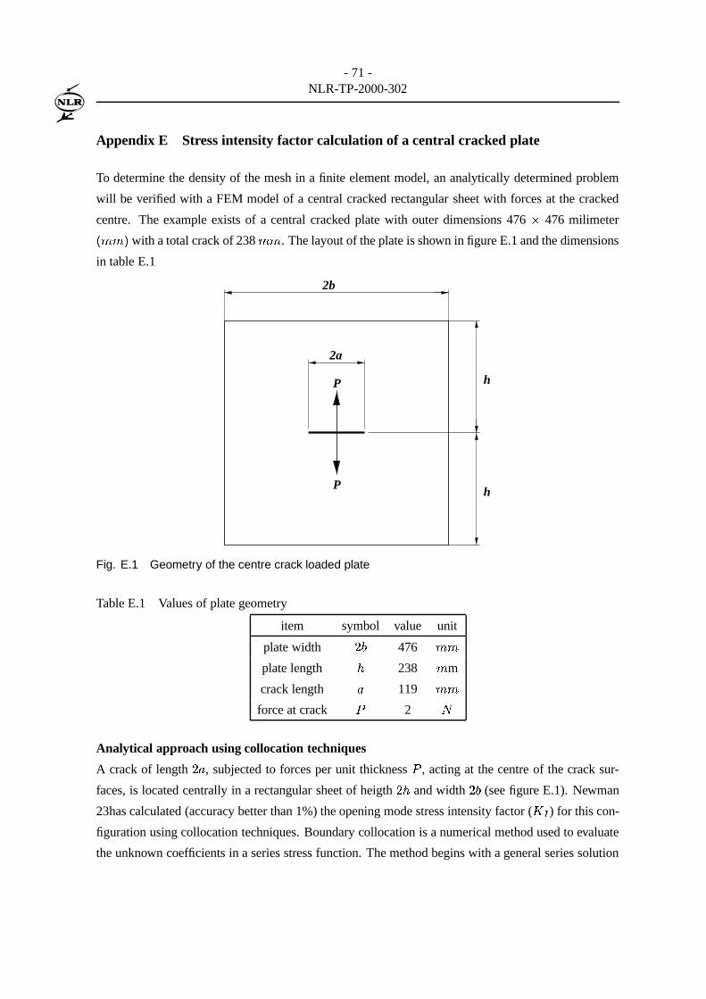
- 71 -NLR-TP-2000-302
Appendix E Stress intensity factor calculation of a central cracked plate
To determine the density of the mesh in a finite element model, an analytically determined problem
will be verified with a FEM model of a central cracked rectangular sheet with forces at the cracked
centre. The example exists of a central cracked plate with outer dimensions 476 + 476 milimeterc ���Ed with a total crack of 238 ��� . The layout of the plate is shown in figure E.1 and the dimensions
in table E.1
2b
2a
P
P h
h
Fig. E.1 Geometry of the centre crack loaded plate
Table E.1 Values of plate geometry
item symbol value unit
plate width� � 476 ���
plate length�
238 � m
crack length 119 ���force at crack
�2 �
Analytical approach using collocation techniques
A crack of length� , subjected to forces per unit thickness
�, acting at the centre of the crack sur-
faces, is located centrally in a rectangular sheet of heigth� �
and width� � (see figure E.1). Newman
23has calculated (accuracy better than 1%) the opening mode stress intensity factor (7�Ð
) for this con-
figuration using collocation techniques. Boundary collocation is a numerical method used to evaluate
the unknown coefficients in a series stress function. The method begins with a general series solution

- 72 -NLR-TP-2000-302
to the governing linear partial equation (see equation E.1).
, 5 c F c $ �"%�d�d s �- 5 F c $ �"%`d- $ 5 } � - 5 F c $ �"%�d- $ , - % , } - 5 F c $ �"%�d- % 5 s � (E.1)
WhereinF c $ �"%�d is the Airy stress funcion. The biharmonic function
F c $ �"%�d can be expressed as
F c $ �"%`d s�f� B M/.10 2 c '�d G 'p}3054 c '_d G 'Ã} c '+� '�d64 c '_d"d87 (E.2)
S R s - , F c $ �"%�d- % ,S R s - , F c $ �"%�d- $ ,W RNa s � - , F c $ �"%�d- $ - % (E.3)
Certain terms are eliminated from the series by conditions of symmetry. The series is then truncated
to a specific number of terms. The coefficients are determined through satisfaction of prescribed
boundary conditions. The series solution obtained satisfies the governing equation in the interior of
the region exactly and one or more of the boundary conditions approximately. Curves of7 Ð H 7 �
versus KH�� for various values of� H�� are shown in figure E.2.
9:;< => ?
@ @BAC9 @DA : @BA ; @DA < @BA = @BA > @BA ? @BA E
� ñ� ¾
P ä� ä sv�Kw±²��� ä sv�KwÛÁ�² � ä s f w´���� ä sé��w´���Fig. E.2
7ÕÐfor a central cracked rectangular sheet with opposing forces at the crack centre

- 73 -NLR-TP-2000-302
Where7 � is defined as the stress intensity factor for an isolated (
� s � s � ) crack subjected to
centrally located opposing forces,�
, is given by;
7 � s �8 � (E.4)
The stress intensity factor of the sheet will be determined with the use of figure E.2, obtained from
ref. 24. In the example �H�� sv�Kw±²and
� H�� s f w´� from which follows that7xÐ H 7 � s f w±æ�° .
7ÕÐ s f w±æ�° � �8 � s �Kw f Á ³ (E.5)
FEM
For the calculation of the stress intensity factor a model of the central loaded cracked plate is nec-
essary. Due to symmetry only a half of the plate can be modelled by using appropiate boundary
conditions. The model is shown in figure E.3. Using the symmetry of the model, the boundray condi-
tions for the section are:� s �� {�q � s �� {�q # s �All geometry data is taken from table E.1.
The stress intensity factor solution is calculated with NASTRAN for several mesh sizes (resp. 6, 12
and 24 elements over crack length), and with B2000 (for 6 elements over crack length). The solutions
are presented in table E.2.
Table E.2 Results of FEM analysis
FEM program elements over crack tip7 Ð
error with respect to coll. techn.
NASTRAN 3 0.154852ò f �bè
NASTRAN 6 0.165799òpæbè
NASTRAN 12 0.170161ò i è
B2000 3 0.170200ò i è
These results show that many elements are needed for NASTRAN, while B2000 only uses few to
obtain solutions with the same deviation. For the calculation of the stress intensity factor solution
of the compressor fan disc NASTRAN will be used due to the inability to use cilindrical coordi-

- 74 -NLR-TP-2000-302
Fig. E.3 Finite Element Model of central loaded and cracked sheet
nate systems in B2000 which are necessary for the construction of the model and for the boundary
conditions. Therefore special care must be taken in the determination of the mesh size within PA-
TRAN/NASTRAN. The assumption is made that, element size =**|, � crack size, to obtain solutions
with rather small deviation.

- 75 -NLR-TP-2000-302
Appendix F FEM calculated stress intensity factor figures
In this appendix, two figures of the SIF solution are presented. The first figure (figure F.1) shows
SIF’s as a function of crack size, with the crack in the direction of the spline and with the crack in the
direction of the support. For reference the NASGRO solution of a bi-axially infinite loaded plate with
a hole is shown. The second figure (figure F.2) shows even more infinite plate solutions and has fitted
curves through the FEM calculated SIF points.
In figure F.2 load cases TC09-bi refers to a bi-axially loaded infinite plate with one hole in the centre.
Load case TC09-un presents the same plate but is uni-axially loaded. The TC03 load cases are uni-
axially loaded plates with infinite length and finite width, with a hole in the centre. These infinite plate
solutions are added to see the influence of the support and the holes in the FEM generated solution.
For large cracks the SIF solution is seen to approach the TC09-bi load case, because the model of the
hub is a cylinder with a uniform stress distribution.

- 76 -NLR-TP-2000-302
Stre
ss in
tens
ity
fact
or s
olut
ion
0123456
02
46
810
1214
crac
k le
ngth
, [m
m]
KI / Snom
FE
M r
esul
ts o
f cra
ck to
spl
ine
FE
M r
esul
ts o
f cra
ck to
sup
port
NA
SG
RO
res
ults
of i
nfin
ite b
iaxi
ally
load
ed p
late
TC
09-b
i
Fig
.F.
1F
EM
calc
ulat
edS
IF

- 77 -NLR-TP-2000-302
Stre
ss in
tens
ity
fact
or s
olut
ions
024681012
02
46
810
12
Cra
ck le
ngth
(m
m)
KI/Snom
TC
09-b
iT
C09
-un
TC
03 W
=75
mm
TC
03 W
=22
.6T
C03
W=
16.1
mm
NA
ST
RA
N S
IF c
rack
to s
uppo
rt
NA
ST
RA
N S
IF c
rack
to s
plin
eF
it of
NA
ST
RA
N S
IF c
rack
to s
uppo
rt s
plin
eF
it of
NA
ST
RA
N S
IF c
rack
to s
uppo
rt s
uppo
rt
Fig
.F.
2F
itted
FE
Mca
lcul
ated
SIF

- 78 -NLR-TP-2000-302
Appendix G C++ programs
In this appendix the C++ programs are listed that were developed for the crack growth calculation
research. The first program listed is the load sequence generator, the second program is the mission
counter.
Load sequence generator program
This program generates a random file of 1000 flights. To create the load sequence, data of the RNLAF
mission mix is inserted in the program. The mission mix is classified, because it can reveal the defence
and training stratagy. The mission mix values are substituted in the program by “XXX”.
#include <stdio.h>
#include <stdlib.h>
#include <iostream.h>
#include <new.h>
#include <limits.h>
int *initial(void);
int *teller(int waarde, int *tell);
int *shuffle(int *row);
int uitvoer(int *rij2, int *rij3);
int memory_error(size_t sz);
int *xpand(int *row2);
int main(void)
{
int
*rij, *rij2, *rij3;
rij = new int [1000];
rij2 = new int [1000];
rij3 = new int [1000];
rij = initial(); //maken van missie vluchten array
rij2 = shuffle(rij); //door elkaar schudden van de missie array
rij3 = xpand(rij2); //uitbreiden naar

- 79 -NLR-TP-2000-302
//vluchten van een bepaalde missie
uitvoer(rij2, rij3);
return(0);
}
int *initial(void)
{
float
recce=XXX, act=XXX, pi=XXX, gf=XXX, range=XXX, agnav=XXX;
// voor XXX relevante waarden invullen
int
*row;
row = new int [1000];
for (int i = 0; i < 1000; i++)
{
if (i < (recce*1000))
row[i] = 1;
if (i < (recce*1000+act*1000) && i >= (recce*1000))
row[i] = 2;
if (i < (recce*1000+act*1000+pi*1000)\
&& i >= (recce*1000+act*1000))
row[i] = 3;
if (i < (recce*1000+act*1000+pi*1000+gf*1000)\
&& i >= (recce*1000+act*1000+pi*1000))
row[i] = 4;
if (i < (recce*1000+act*1000+pi*1000+gf*1000+range*1000)\
&& i >= (recce*1000+act*1000+pi*1000+gf*1000))
row[i] = 5;
if (i < \
(recce*1000+act*1000+pi*1000+gf*1000+range*1000+agnav*1000)\
&& i >= (recce*1000+act*1000+pi*1000+gf*1000+range*1000))
row[i] = 6;
}

- 80 -NLR-TP-2000-302
return(row);
}
int *shuffle(int *row)
{
int
*row2, i, j;
row2 = new int [1000];
j = (1000*rand())/RAND_MAX;
//hierdoor ontstaat een random getal tussen 0 en 1000
for (i = 0; i < 1000; i++)
{
do j = (1000*rand())/RAND_MAX;
while (row[j-1] == 0);
row2[i] = row[j-1];
row[j-1] = 0;
}
return(row2);
}
int *xpand(int *row2)
{
int
k, nflights[6]={5,6,3,1,3,2}, *row3;
row3 = new int [1000]; //hierin komen alleen de sub-vluchten
for (k = 0; k < 1000; k++)
{
if (row2[k] == 1)
{
//random waarde genereren uit 5 vluchten

- 81 -NLR-TP-2000-302
row3[k] = (((nflights[0]-1)*rand())/RAND_MAX)+1;;
}
else
{
if (row2[k] == 2)
{
//random waarde genereren uit 6 vluchten
row3[k] = (((nflights[1]-1)*rand())/RAND_MAX)+1;
}
else
{
if (row2[k] == 3)
{
//random waarde genereren uit 3 vluchten
row3[k] = (((nflights[2]-1)*rand())\
/RAND_MAX)+1;
}
else
{
if (row2[k] == 4)
{
//random waarde genereren uit 1 vlucht
row3[k] = (((nflights[3]-1)*rand())\
/RAND_MAX)+1;
}
else
{
if (row2[k] == 5)
{
//random waarde genereren uit 3 vluchten
row3[k] = (((nflights[4]-1)*rand())\
/RAND_MAX)+1;
}
else
{
if (row2[k] == 6)
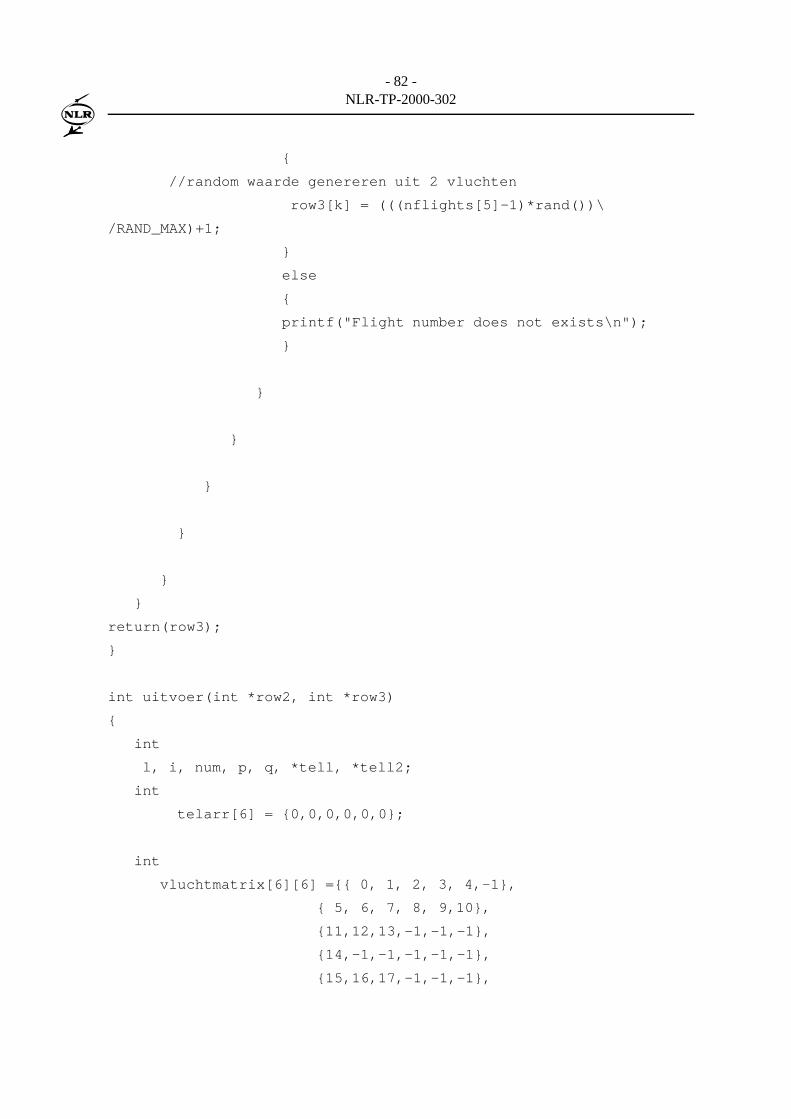
- 82 -NLR-TP-2000-302
{
//random waarde genereren uit 2 vluchten
row3[k] = (((nflights[5]-1)*rand())\
/RAND_MAX)+1;
}
else
{
printf("Flight number does not exists\n");
}
}
}
}
}
}
}
return(row3);
}
int uitvoer(int *row2, int *row3)
{
int
l, i, num, p, q, *tell, *tell2;
int
telarr[6] = {0,0,0,0,0,0};
int
vluchtmatrix[6][6] ={{ 0, 1, 2, 3, 4,-1},
{ 5, 6, 7, 8, 9,10},
{11,12,13,-1,-1,-1},
{14,-1,-1,-1,-1,-1},
{15,16,17,-1,-1,-1},

- 83 -NLR-TP-2000-302
{18,19,-1,-1,-1,-1}};
char
*getal, **fname;
FILE
*infile[20], *outfile;
tell = new int [6];
tell2 = new int [6];
getal = new char [15];
fname = new char* [6];
tell = telarr;
fname[ 0] = "F001.txt"; //RECCE 1
fname[ 1] = "F002.txt"; //RECCE 2
fname[ 2] = "F003.txt"; //RECCE 3
fname[ 3] = "F004.txt"; //RECCE 4
fname[ 4] = "F009.txt"; //RECCE 5
fname[ 5] = "F005.txt"; //ACT 1
fname[ 6] = "F006.txt"; //ACT 2
fname[ 7] = "F007.txt"; //ACT 3
fname[ 8] = "F008.txt"; //ACT 4
fname[ 9] = "F010.txt"; //ACT 5
fname[10] = "F011.txt"; //ACT 6
fname[11] = "F053.txt"; //PI 1
fname[12] = "F057.txt"; //PI 2
fname[13] = "F088.txt"; //PI 3
fname[14] = "F071.txt"; //GF 1
fname[15] = "F063.txt"; //RANGE 1
fname[16] = "F066.txt"; //RANGE 2

- 84 -NLR-TP-2000-302
fname[17] = "F099.txt"; //RANGE 3
fname[18] = "F065.txt"; //AGNAV 1
fname[19] = "F077.txt"; //AGNAV 2
for (p = 0; p < 6; p++)
{
for (q = 0; q < 6; q++)
{
if (vluchtmatrix[p][q] != -1)
{
num = vluchtmatrix[p][q];
if (!(infile[num] = fopen (fname[num], "r")))
{
cout << "Kan Flight" << (i+1)\
<< ".txt niet openen\n";
exit(1);
}
}
}
}
if (!(outfile = fopen ("result.txt", "a")))
{
cout << "Kan result.txt niet openen\n";
exit(1);
}
// voor elk cijfer n in row2 goede file kopieren naar outfile:
for (i = 0; i < 1000; i++)
{
p = row2[i]-1;
tell2 = teller(p+1, tell);
tell = tell2;
q = row3[i]-1;
num = vluchtmatrix[p][q];

- 85 -NLR-TP-2000-302
printf("row2,row3,file = %d,%d,%s\n",row2[i],row3[i]\
,fname[num]);
fprintf(outfile, "%s", "0\n");
// kopieren van een inputfile naar outfile :
fseek(infile[num], 0, 0);
while (fscanf(infile[num], "%s", getal) != EOF)
{
if (fprintf(outfile, "%s", getal) == EOF)
cout << "Foutje bij schrijven naar outfile";
fprintf(outfile, "%s", "\n");
}
}
//nu nog een 0 toevoegen na laatste file
fprintf(outfile, "%s", "0\n");
for (l = 0; l < 20; l++)
{
fclose(infile[l]);
}
fclose(outfile);
cout << "\nAantal 1:" << tell[0];
cout << "\nAantal 2:" << tell[1];
cout << "\nAantal 3:" << tell[2];
cout << "\nAantal 4:" << tell[3];
cout << "\nAantal 5:" << tell[4];
cout << "\nAantal 6:" << tell[5];
return(0);
}
int *teller(int waarde, int *tell)
{
switch ( waarde )

- 86 -NLR-TP-2000-302
{
case 1 :
{
tell[0] += 1;
break;
}
case 2 :
{
tell[1] += 1;
break;
}
case 3 :
{
tell[2] += 1;
break;
}
case 4 :
{
tell[3] += 1;
break;
}
case 5 :
{
tell[4] += 1;
break;
}
case 6 :
{
tell[5] += 1;
break;
}
default :
{
cout << "Geen 1, 2, 3, ,5 of 6 !!\n";
break;

- 87 -NLR-TP-2000-302
}
}
return(tell);
}
Mission counter
To determine in which one of the thousand flights the crack growth calculation is cut off, the following
program is used. The input of this program is the line number where the crack growth calculation has
stopped, which is reported by the crack growth calculation program. The output is the number of
passed flights and the flight number where the calculation is cut off.
#include <stdio.h>
#include <stdlib.h>
#include <iostream.h>
#include <new.h>
#include <limits.h>
int main(void)
{
int
zoekregel, vluchtteller, regelteller;
int
con_ok;
float
*getal;
char
*fname;
FILE
*infile;
getal=new float [15];
fname="result.sf";
if (!(infile = fopen (fname, "r")))
{
printf("Kan %s niet openen !!!\n", fname);

- 88 -NLR-TP-2000-302
exit(1);
}
//read first value of result.sf
fseek(infile,0,0);
regelteller = 1;
vluchtteller = 0;
printf("Enter het regelnummer waar CRAGRO berekening de ");
printf("maximale scheurlengte overschreed.\n");
con_ok=scanf("%d",&zoekregel);
if (con_ok != 1)
printf("mislukt geen 1 integers gelezen");
printf("Regel waarop gezocht wordt = %d\n",zoekregel);
while ((fscanf(infile,"%f",getal) != EOF)\
&& (zoekregel != regelteller))
{
// printf("getal = %f\n",getal);
if (*getal == 0)
{
vluchtteller = vluchtteller + 1;
printf("regel = %d\n",regelteller);
printf("vlucht = %d\n",vluchtteller);
}
regelteller = regelteller + 1;
}
fclose(infile);
//uitvoer
printf("Invoer regelnummer = %d\n",zoekregel);
printf("Gestopt bij regelnummer = %d\n",regelteller);
printf("Aantal doorlopen vluchten = %d\n",vluchtteller-1);
printf("Gestopt in vlucht = %d\n",vluchtteller);

- 89 -NLR-TP-2000-302
return(0);
}

- 90 -NLR-TP-2000-302
Appendix H Fitting crack growth data
To produce the fit for the materials crack growth curve, a Microsoft Excel sheet is written which
processes crack growth data to a form usable for a commercial datafit program. (Instructions are
given on the first data sheet of the Excel program) The items the user has to enter are: materials crack
growth data points and common data, which units are used. When these data are entered, a macro
must be activated, which will process the data into a form usable for the datafit program. When this
macro has completed the converted data can be copied to the commercial datafit program. To obtain
the fit first a general equation must be generated to which the data must be fitted. Such an equation
has the following form:
G G � s c Z 7 �ÌÊËÊ d ä � f � <��� Í?Î(Î � �� f � ��� Í?Î(Î� � Ê (H.1)
Where� P�GF equals Y and
Z 7 �zÊhÊ equals X, and the letters a through z represent the fit constants. This
equation is just an example, other, more complex equations are possible (taking e.g. the stress ratio
and the crack opnening function into account).

- 91 -NLR-TP-2000-302
Appendix I Implementation of CRAC2D elements in NASTRAN input files
Introduction
When engineering fracture mechanics, finite element models are frequently used to calculate stress
intensity factors. The finite element program NASTRAN of the MacNeal-Schwendler corporation
is capable to produce stress intensity factors because special cracktip elements are programmed. To
use the special cracktip elements, PATRAN (the pre- and post processor) cannot be used, because it
does not support cracktip elements. To implement these special cracktip elements in cracked finite
element models, the bulk data deck (this is a file containing the code of the model) has to be altered.
Difficulties were encountered using the cracktip elements. Therefore a description of the use of the
special cracktip elements is added to this report.
Applying CRAC2D elements
To use CRAC2D elements in a model, some details have to be considered. First, when building the
geometry of the model in a pre-processor like PATRAN, special interest must be taken in the vicinity
of the tip of the crack. When building the geometry, a square surface of approximately 1 IJ� , must be
modelled with the centre of the square as the tip of the crack. Brake this surface with a modelled crack,
so that two rectangels are obtained. Mesh these surfaces to obtain square elements (four- or eigth node
elements), using an even mesh seed on the long side of the rectangle (e.g. 10) and half of the long
side mesh seed for the short side of the rectangle (e.g. 5). Delete the four elements surrounding the
tip of the crack, without deleting the nodes. With the EQUIVALENCE option, all double nodes (not for
the crack) must be deleted. With the option SHOW, the outer node numbers and the centre (cracktip)
node of the 4 deleted elements must be obtained and reported on paper. Using four node elements, 10
nodes must be reported (G1 through G10). Using eight node elements, 18 nodes must be reported (G1
through G18). See figure I.1 This ends the work in the pre-prossor, so make a NASTRAN analysis
deck of the model to obtain the bulk data deck file (filename.bdf ).
From the NASTRAN analysis deck (filename.bdf ) some key elements have to be added to produce
the analysis deck with the crack tip elements. These are:
- ADUMi element, defines attributes of the dummy element;
- PRAC2D, defines properties of the crack tip element;
- CRAC2D, defines two-dimensional crack tip element.
HADUMi
This element is called a dummy element. This dummy element contains information about the amount

- 92 -NLR-TP-2000-302
G13 G5
G14
G6
G4
x
y
G1
G12
G15
G10
G2
G9
G3
G18
G7G16G17 G8
G11
Fig. I.1 NASTRAN cracktip element
of grid points of the cracktip element, and the number of additional fields for other entries. The format
of this element is shown in table I.1. Fill in this element the total number of nodes usually 18 or 10,
and the name of the element type (in this case CRAC2D).
ADUMi NG NC NP ND ELNM - - - -
NG Number of grid point connected by DUMi element
NC Number of add. fields on CDUM connection entry
NP Number of add. fields on the PDUMi prop. entry
ND Number of displacement compo. at each grid point
ELNM Name of element connection
Table I.1 Format ADUMiHPRAC2D
This command is used to define the element properties of the cracktip element. The format of this
command is shown in table I.2. This command is used to give the cracktip element a specific thickness,
wich must be equivalent to the thickness of the shells surrounding the cracktip element. With the
IPLANE option it is possible to define the state of stress. Use 0 for plane strain; 1 for plane stress.
Use for the GAMMA and the PHI option the default value, because non-default values are not tested
by NASTRAN yet.HCRAC2D

- 93 -NLR-TP-2000-302
PRAC2D PID MID T IPLANE NSM GAMMA PHI - -
PID Property id number of PRAC2D entry
MID Material id number
T Thickness
IPLANE Plain stress/strain option
NSM Non-Structural Mass per unit area Default=0
GAMMA Default=0.5
PHI Default=180.0
Table I.2 Format PRAC2D
This command is used to define the cracktip element. The format of this element is shown in table
I.3. The reported node numbers from PATRAN correspond with G1 through G18 in the CRAC2D
command.
CRAC2D EID PID G1 G2 G3 G4 G5 G6
G7 G8 G9 G10 G11 G12 G13 G14
G15 G16 G17 G18
EID Element id number
PID Property id number of PRAC2D entry
Gi Grid point id number
Table I.3 Format CRAC2D
The description of the 3 command are necessary to use cracktip elements in a finite element model.
The following lines are taken from a from a bulk data deck file of a cracked hub.
ADUM8 18 0 5 0 CRAC2D
PRAC2D 999 1 7.45 1 0 0.50 180.
CRAC2D 1322 999 1128 1236 1268 1266 1264 1111 + ZZZ1
+ ZZZ1 1113 1130 1147 1145 1251 1267 1265 1249 + ZZZ2
+ ZZZ2 1112 1123 1140 1146
In this case the element number is 1322 with material properties 999. A plane stress analysis will be
carried out on an element with a thickness of 7.45 ��� . The ADUM8 element specifies 18 nodes,
which are filled in the CRAC2D command (beginning with 1128 ... ending with 1146). Note that the
node numbers correspond with the right IKJ numbers. The }MLNLOL P statements are used because one
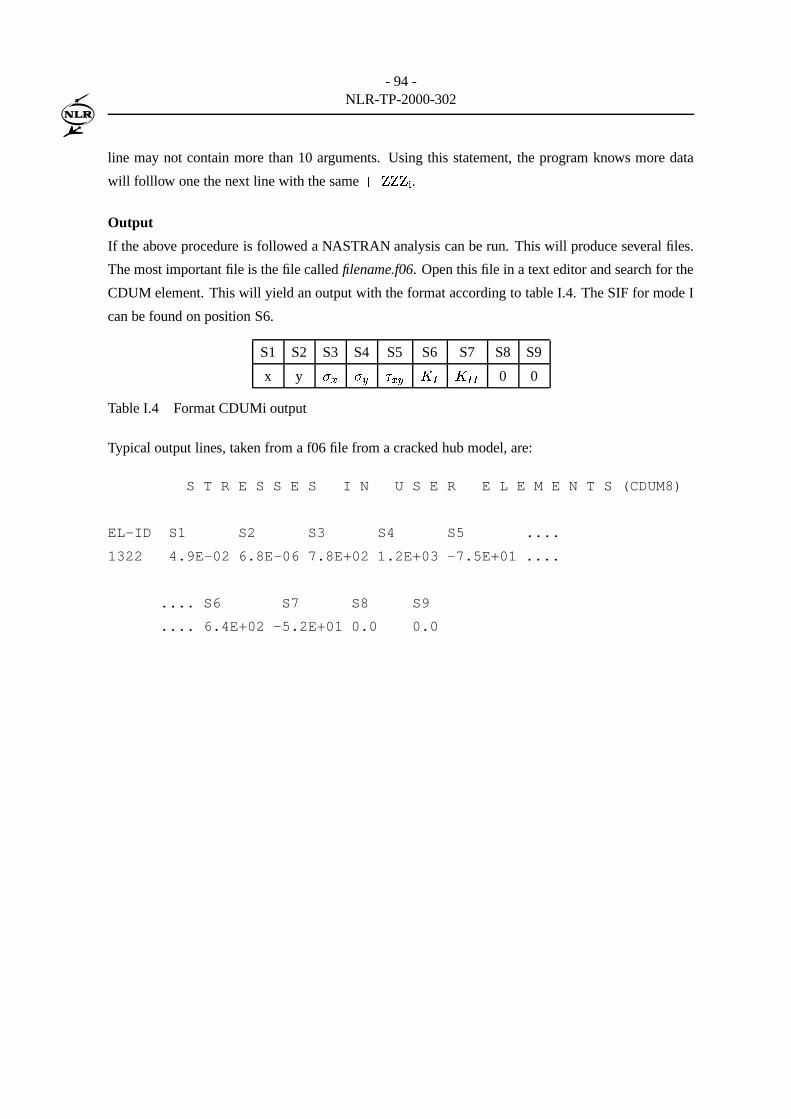
- 94 -NLR-TP-2000-302
line may not contain more than 10 arguments. Using this statement, the program knows more data
will folllow one the next line with the same }MLNLOL P .Output
If the above procedure is followed a NASTRAN analysis can be run. This will produce several files.
The most important file is the file called filename.f06. Open this file in a text editor and search for the
CDUM element. This will yield an output with the format according to table I.4. The SIF for mode I
can be found on position S6.
S1 S2 S3 S4 S5 S6 S7 S8 S9
x y S R S a W RNa 7¢Ð 7¢Ð�Ð0 0
Table I.4 Format CDUMi output
Typical output lines, taken from a f06 file from a cracked hub model, are:
S T R E S S E S I N U S E R E L E M E N T S (CDUM8)
EL-ID S1 S2 S3 S4 S5 ....
1322 4.9E-02 6.8E-06 7.8E+02 1.2E+03 -7.5E+01 ....
.... S6 S7 S8 S9
.... 6.4E+02 -5.2E+01 0.0 0.0