Embed Size (px)
Citation preview
Recommendation ITU-R P.618-11 (09/2013)
Propagation data and prediction methods required for the design of Earth-space
telecommunication systems
P Series
Radiowave propagation
ii Rec. ITU-R P.618-11
Foreword
The role of the Radiocommunication Sector is to ensure the rational, equitable, efficient and economical use of the
radio-frequency spectrum by all radiocommunication services, including satellite services, and carry out studies without
limit of frequency range on the basis of which Recommendations are adopted.
The regulatory and policy functions of the Radiocommunication Sector are performed by World and Regional
Radiocommunication Conferences and Radiocommunication Assemblies supported by Study Groups.
Policy on Intellectual Property Right (IPR)
ITU-R policy on IPR is described in the Common Patent Policy for ITU-T/ITU-R/ISO/IEC referenced in Annex 1 of
Resolution ITU-R 1. Forms to be used for the submission of patent statements and licensing declarations by patent
holders are available from http://www.itu.int/ITU-R/go/patents/en where the Guidelines for Implementation of the
Common Patent Policy for ITU-T/ITU-R/ISO/IEC and the ITU-R patent information database can also be found.
Series of ITU-R Recommendations
(Also available online at http://www.itu.int/publ/R-REC/en)
Series Title
BO Satellite delivery
BR Recording for production, archival and play-out; film for television
BS Broadcasting service (sound)
BT Broadcasting service (television)
F Fixed service
M Mobile, radiodetermination, amateur and related satellite services
P Radiowave propagation
RA Radio astronomy
RS Remote sensing systems
S Fixed-satellite service
SA Space applications and meteorology
SF Frequency sharing and coordination between fixed-satellite and fixed service systems
SM Spectrum management
SNG Satellite news gathering
TF Time signals and frequency standards emissions
V Vocabulary and related subjects
Note: This ITU-R Recommendation was approved in English under the procedure detailed in Resolution ITU-R 1.
Electronic Publication
Geneva, 2013
ITU 2013
All rights reserved. No part of this publication may be reproduced, by any means whatsoever, without written permission of ITU.
Rec. ITU-R P.618-11 1
RECOMMENDATION ITU-R P.618-11
Propagation data and prediction methods required for the design
of Earth-space telecommunication systems
(Question ITU-R 206/3)
(1986-1990-1992-1994-1995-1997-1999-2001-2003-2007-2009-2013)
Scope
This Recommendation predicts the various propagation parameters needed in planning Earth-space systems
operating in either the Earth-to-space or space-to-Earth direction.
The ITU Radiocommunication Assembly,
considering
a) that for the proper planning of Earth-space systems, it is necessary to have appropriate
propagation data and prediction techniques;
b) that methods have been developed that allow the prediction of the most important
propagation parameters needed in planning Earth-space systems;
c) that as far as possible, these methods have been tested against available data and have been
shown to yield an accuracy that is both compatible with the natural variability of propagation
phenomena and adequate for most present applications in system planning,
recommends
that the methods for predicting the propagation parameters set out in Annex 1 should be adopted for
planning Earth-space radiocommunication systems, in the respective ranges of validity indicated in
Annex 1.
NOTE 1 – Supplementary information related to the planning of broadcasting-satellite systems as
well as maritime, land, and aeronautical mobile-satellite systems, may be found in
Recommendations ITU-R P.679, ITU-R P.680, ITU-R P.681 and ITU-R P.682, respectively.
2 Rec. ITU-R P.618-11
Annex 1
1 Introduction
In the design of Earth-space links for communication systems, several effects must be considered.
Effects of the non-ionized atmosphere need to be considered at all frequencies, but become critical
above about 1 GHz and for low elevation angles. These effects include:
a) absorption in atmospheric gases; absorption, scattering and depolarization by hydrometeors
(water and ice droplets in precipitation, clouds, etc.); and emission noise from absorbing
media; all of which are especially important at frequencies above about 10 GHz;
b) loss of signal due to beam-divergence of the earth-station antenna, due to the normal
refraction in the atmosphere;
c) a decrease in effective antenna gain, due to phase decorrelation across the antenna aperture,
caused by irregularities in the refractive-index structure;
d) relatively slow fading due to beam-bending caused by large-scale changes in refractive
index; more rapid fading (scintillation) and variations in angle of arrival, due to small-scale
variations in refractive index;
e) possible limitations in bandwidth due to multiple scattering or multipath effects, especially
in high-capacity digital systems;
f) attenuation by the local environment of the ground terminal (buildings, trees, etc.);
g) short-term variations of the ratio of attenuations at the up- and down-link frequencies,
which may affect the accuracy of adaptive fade countermeasures;
h) for non-geostationary satellite (non-GSO) systems, the effect of varying elevation angle to
the satellite.
Ionospheric effects (see Recommendation ITU-R P.531) may be important, particularly at
frequencies below 1 GHz. For convenience these have been quantified for frequencies of 0.1; 0.25;
0.5; 1; 3 and 10 GHz in Table 1 for a high value of total electron content (TEC). The effects
include:
j) Faraday rotation: a linearly polarized wave propagating through the ionosphere undergoes a
progressive rotation of the plane of polarization;
k) dispersion, which results in a differential time delay across the bandwidth of the transmitted
signal;
l) excess time delay;
m) ionospheric scintillation: inhomogeneities of electron density in the ionosphere cause
refractive focusing or defocusing of radio waves and lead to amplitude fluctuations termed
scintillations. Ionospheric scintillation is maximum near the geomagnetic equator and
smallest in the mid-latitude regions. The auroral zones are also regions of large scintillation.
Strong scintillation is Rayleigh distributed in amplitude; weaker scintillation is nearly
log-normal. These fluctuations decrease with increasing frequency and depend upon path
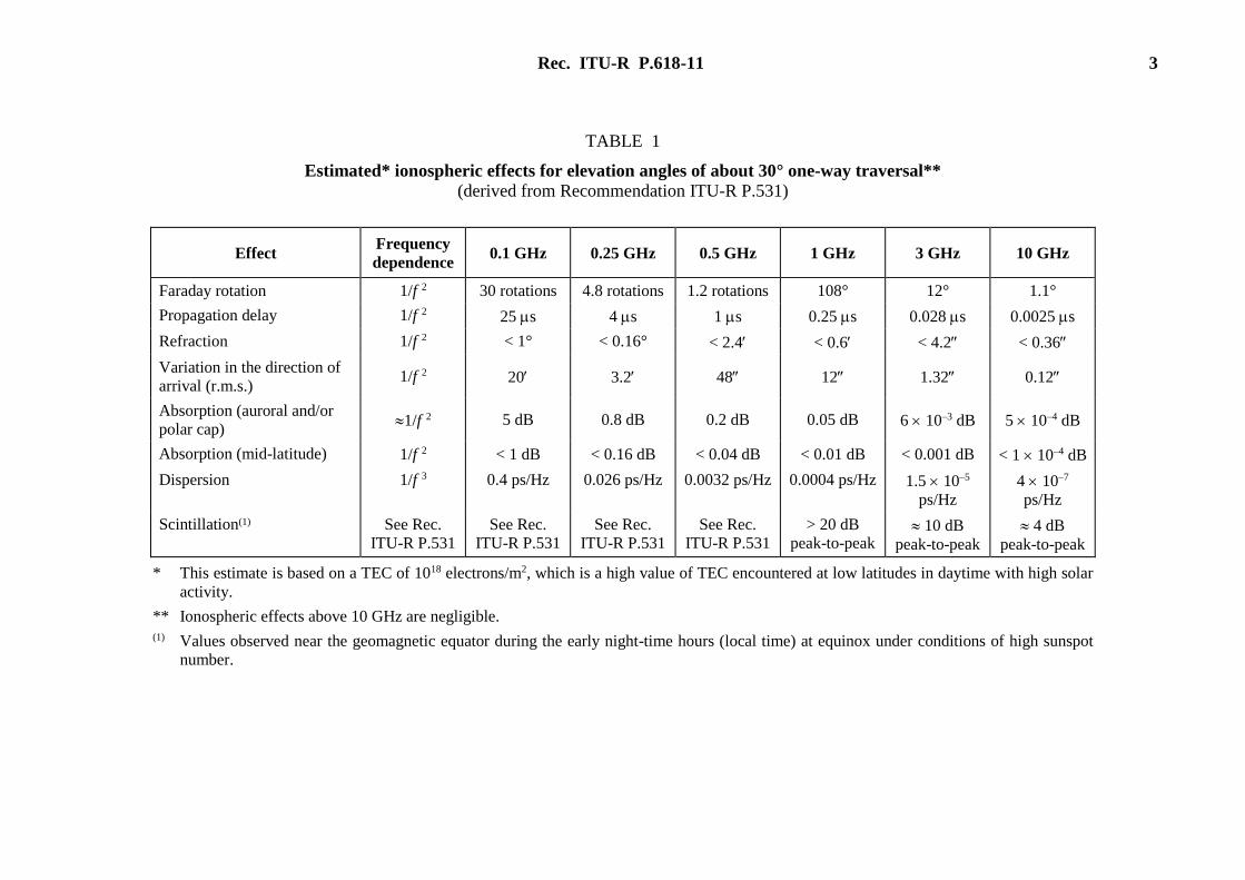
geometry, location, season, solar activity and local time. Table 2 tabulates fade depth data
for VHF and UHF in mid-latitudes, based on data in Recommendation ITU-R P.531.
Accompanying the amplitude fluctuation is also a phase fluctuation. The spectral density of
the phase fluctuation is proportional to 1/f 3, where f is the Fourier frequency of the
fluctuation. This spectral characteristic is similar to that arising from flicker of frequency in
oscillators and can cause significant degradation to the performance of receiver hardware.
Rec. ITU-R P.618-11 3
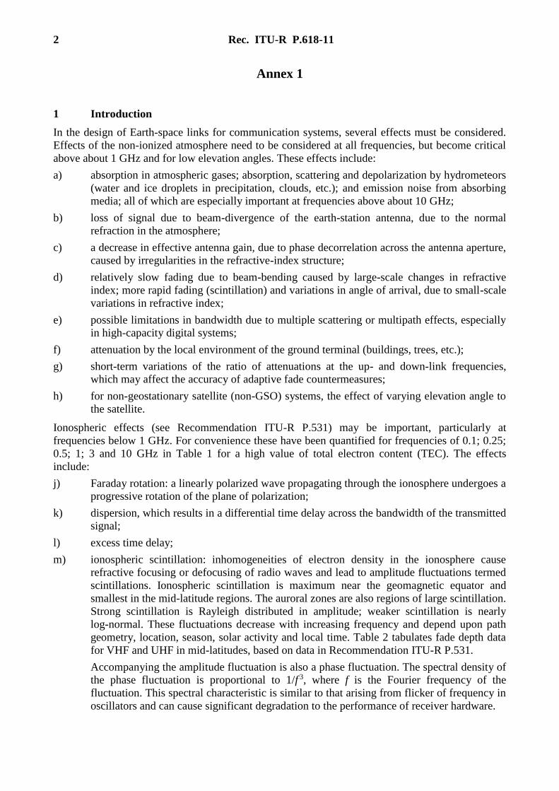
TABLE 1
Estimated* ionospheric effects for elevation angles of about 30° one-way traversal**
(derived from Recommendation ITU-R P.531)
Effect Frequency
dependence 0.1 GHz 0.25 GHz 0.5 GHz 1 GHz 3 GHz 10 GHz
Faraday rotation 1/f 2 30 rotations 4.8 rotations 1.2 rotations 108° 12° 1.1°
Propagation delay 1/f 2 25 s 4 s 1 s 0.25 s 0.028 s 0.0025 s
Refraction 1/f 2 < 1° < 0.16° < 2.4 < 0.6 < 4.2 < 0.36
Variation in the direction of
arrival (r.m.s.) 1/f 2 20 3.2 48 12 1.32 0.12
Absorption (auroral and/or
polar cap) 1/f 2 5 dB 0.8 dB 0.2 dB 0.05 dB 6 10–3 dB 5 10–4 dB
Absorption (mid-latitude) 1/f 2 < 1 dB < 0.16 dB < 0.04 dB < 0.01 dB < 0.001 dB < 1 10–4 dB
Dispersion 1/f 3 0.4 ps/Hz 0.026 ps/Hz 0.0032 ps/Hz 0.0004 ps/Hz 1.5 10–5
ps/Hz
4 10–7
ps/Hz
Scintillation(1) See Rec.
ITU-R P.531
See Rec.
ITU-R P.531
See Rec.
ITU-R P.531
See Rec.
ITU-R P.531
> 20 dB
peak-to-peak 10 dB
peak-to-peak
4 dB
peak-to-peak
* This estimate is based on a TEC of 1018 electrons/m2, which is a high value of TEC encountered at low latitudes in daytime with high solar
activity.
** Ionospheric effects above 10 GHz are negligible.
(1) Values observed near the geomagnetic equator during the early night-time hours (local time) at equinox under conditions of high sunspot
number.
4 Rec. ITU-R P.618-11
TABLE 2
Distribution of mid-latitude fade depths due to ionospheric scintillation (dB)
This Annex deals only with the effects of the troposphere on the wanted signal in relation to system
planning. Interference aspects are treated in separate Recommendations:
– interference between earth stations and terrestrial stations (Recommendation ITU-R P.452);
– interference from and to space stations (Recommendation ITU-R P.619);
– bidirectional coordination of earth stations (Recommendation ITU-R P.1412).
An apparent exception is path depolarization which, although of concern only from the standpoint
of interference (e.g. between orthogonally-polarized signal transmissions), is directly related to the
propagation impairments of the co-polarized direct signal.
The information is arranged according to the link parameters to be considered in actual system
planning, rather than according to the physical phenomena causing the different effects. As far as
possible, simple prediction methods covering practical applications are provided, along with
indications of their range of validity. These relatively simple methods yield satisfactory results in
most practical applications, despite the large variability (from year to year and from location to
location) of propagation conditions.
As far as possible, the prediction methods in this Annex have been tested against measured data
from the data banks of Radiocommunication Study Group 3 (see Recommendation ITU-R P.311).
2 Propagation loss
The propagation loss on an Earth-space path, relative to the free-space loss, is the sum of different
contributions as follows:
– attenuation by atmospheric gases;
– attenuation by rain, other precipitation and clouds;
– focusing and defocusing;
– decrease in antenna gain due to wave-front incoherence;
– scintillation and multipath effects;
– attenuation by sand and dust storms.
Each of these contributions has its own characteristics as a function of frequency, geographic
location and elevation angle. As a rule, at elevation angles above 10°, only gaseous attenuation, rain
and cloud attenuation and possibly scintillation will be significant, depending on propagation
conditions. For non-GSO systems, the variation in elevation angle should be included in the
calculations, as described in § 8.
Percentage of time
(%)
Frequency
(GHz)
0.1 0.2 0.5 1
1 5.9 1.5 0.2 0.1
0.5 9.3 2.3 0.4 0.1
0.2 16.6 4.2 0.7 0.2
0.1 25 6.2 1 0.3
Rec. ITU-R P.618-11 5
(In certain climatic zones, snow and ice accumulations on the surfaces of antenna reflectors and
feeds can produce prolonged periods with severe attenuation, which might dominate even the
annual cumulative distribution of attenuation.)
2.1 Attenuation due to atmospheric gases
Attenuation by atmospheric gases which is entirely caused by absorption depends mainly on
frequency, elevation angle, altitude above sea level and water vapour density (absolute humidity).
At frequencies below 10 GHz, it may normally be neglected. Its importance increases with
frequency above 10 GHz, especially for low elevation angles. Annex 1 of Recommendation
ITU-R P.676 gives a complete method for calculating gaseous attenuation, while Annex 2 of the
same Recommendation gives an approximate method for frequencies up to 350 GHz.
At a given frequency the oxygen contribution to atmospheric absorption is relatively constant.
However, both water vapour density and its vertical profile are quite variable. Typically, the
maximum gaseous attenuation occurs during the season of maximum rainfall (see
Recommendation ITU-R P.836).
2.2 Attenuation by precipitation and clouds
2.2.1 Prediction of attenuation statistics for an average year
The general method to predict attenuation due to precipitation and clouds along a slant propagation
path is presented in § 2.2.1.1.
If reliable long-term statistical attenuation data are available that were measured at an elevation
angle and a frequency (or frequencies) different from those for which a prediction is needed, it is
often preferable to scale these data to the elevation angle and frequency in question rather than
using the general method. The recommended frequency-scaling method is found in § 2.2.1.2.
Site diversity effects may be estimated with the method of § 2.2.4.
2.2.1.1 Calculation of long-term rain attenuation statistics from point rainfall rate
The following procedure provides estimates of the long-term statistics of the slant-path rain
attenuation at a given location for frequencies up to 55 GHz. The following parameters are required:
R0.01 : point rainfall rate for the location for 0.01% of an average year (mm/h)
hs: height above mean sea level of the earth station (km)
: elevation angle (degrees)
: latitude of the earth station (degrees)
f: frequency (GHz)
Re: effective radius of the Earth (8 500 km).
If local data for the earth station height above mean sea level is not available, an estimate can be
obtained from the maps of topographic altitude given in Recommendation ITU-R P.1511.
The geometry is illustrated in Fig. 1.
6 Rec. ITU-R P.618-11
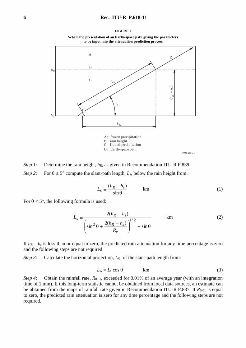
FIGURE 1
Schematic presentation of an Earth-space path giving the parameters
to be input into the attenuation prediction process
P.0618-01
A: frozen precipitationB: rain heightC: liquid precipitation
D: Earth-space path
B
AD
C
hR
hs
LG
L s
()
h
– h
Rs
Step 1: Determine the rain height, hR, as given in Recommendation ITU-R P.839.
Step 2: For 5° compute the slant-path length, Ls, below the rain height from:
kmsin
)(
sRs
hhL (1)
For < 5°, the following formula is used:
km
sin)(2
sin
)(2
2/12
e
sR
sRs
R
hh
hhL (2)
If hR – hs is less than or equal to zero, the predicted rain attenuation for any time percentage is zero
and the following steps are not required.
Step 3: Calculate the horizontal projection, LG, of the slant-path length from:
LG = Ls cos km (3)
Step 4: Obtain the rainfall rate, R0.01, exceeded for 0.01% of an average year (with an integration
time of 1 min). If this long-term statistic cannot be obtained from local data sources, an estimate can
be obtained from the maps of rainfall rate given in Recommendation ITU-R P.837. If R0.01 is equal
to zero, the predicted rain attenuation is zero for any time percentage and the following steps are not
required.
Rec. ITU-R P.618-11 7
Step 5: Obtain the specific attenuation, R, using the frequency-dependent coefficients given in
Recommendation ITU-R P.838 and the rainfall rate, R0.01, determined from Step 4, by using:
R = k (R0.01) dB/km (4)
Step 6: Calculate the horizontal reduction factor, r0.01, for 0.01% of the time:
GLRG
f
Lr
201.0
e138.078.01
1
(5)
Step 7: Calculate the vertical adjustment factor, v0.01, for 0.01% of the time:
degrees–
tan01.0
1–
rL
hh
G
sR
For > , kmcos
01.0
rLL G
R
Else, kmsin
)–(
sRR
hhL
If | | < 36°, = 36 – | | degrees
Else, = 0 degrees
45.0–e–131sin1
1ν
2
)1/(–
01.0
f
L RR
Step 8: The effective path length is:
LE = LR 0.01 km (6)
Step 9: The predicted attenuation exceeded for 0.01% of an average year is obtained from:
A0.01 = R LE dB (7)
Step 10: The estimated attenuation to be exceeded for other percentages of an average year, in the
range 0.001% to 5%, is determined from the attenuation to be exceeded for 0.01% for an average
year:
If p 1% or || 36°: = 0
If p < 1% and || < 36° and 25°: = –0.005(|| – 36)
Otherwise: = –0.005(|| – 36) + 1.8 – 4.25 sin
dB01.0
)sin)–1(–)n(10.045–)n(1033.0655.0–(
01.0
01.0
pAp
pp
AA (8)
This method provides an estimate of the long-term statistics of attenuation due to rain. When
comparing measured statistics with the prediction, allowance should be given for the rather large
year-to-year variability in rainfall rate statistics (see Recommendation ITU-R P.678).
8 Rec. ITU-R P.618-11
2.2.1.2 Frequency scaling of rain attenuation
Frequency scaling is the prediction of a propagation effect (e.g. rain attenuation) at one frequency
from knowledge of the propagation effect at a different frequency. Typically, the frequency of the
predicted propagation effect is higher than the frequency of the known propagation effect. The ratio
between the rain attenuation at the two frequencies can vary during a rain event, and the variability
of the ratio generally increases as the rain attenuation increases.
Two prediction methods are provided in the following paragraphs:
1) Section 2.2.1.2.1 provides a method of predicting the statistical variation of the rain
attenuation at frequency f2 conditioned on the rain attenuation at frequency f1. This method
requires the cumulative distributions of rain attenuation at both frequencies.
2) Section 2.2.1.2.2 provides a simplified method of predicting the equiprobable rain
attenuation at frequency f2 conditioned on the rain attenuation at frequency f1. This method
does not require the cumulative distribution of the rain attenuation at either frequency.
These prediction methods may be applicable to uplink power control and adaptive coding and
modulation, for example:
a) The first method predicts the instantaneous uplink rain attenuation at frequency f2 based on
the measured instantaneous downlink rain attenuation at frequency f1 for a p% risk the
actual uplink rain attenuation will exceed the predicted value.
b) The second method predicts the uplink rain attenuation at frequency f2 based on knowledge
of the downlink rain attenuation at frequency f1 at the same probability of exceedance.
2.2.1.2.1 Conditional distribution of the frequency scaling ratio of rain attenuation
This prediction method is based on the following relation between A2 (dB), the instantaneous rain
attenuation at frequency f2, and A1 (dB), the instantaneous rain attenuation at frequency f1.
nAA
ξσξ1
σ
μσμlnξ1
σ
σ)ln( 2
2
1
1221
2
1
22
(9)
where n is a normal distribution with zero mean and unit variance. The following step-by-step
procedure predicts 1122 aAaAP , the complementary cumulative distribution function of the
rain attenuation at frequency f2 conditioned on the rain attenuation at frequency f1.
This method assumes 0111 AaAP and 0222 AaAP , the complementary cumulative
distributions of rain attenuation conditioned on the occurrence of non-zero rain attenuation on the
path at frequencies f1 and f2 are characterized by log-normal distributions with parameters 11 σ,μ
and 22 σ,μ :
1
11111
σ
μln0
aQAaAP (10a)
2
22222
σ
μln0
aQAaAP (10b)
where:
x
t
txQ deπ2
12
2
(11)
The parameters 1, 1, 2 and 2 are derived from the rain attenuation statistics at frequencies f1 and
f2 for the same propagation path. These rain attenuation statistics can be computed from the local
measured rain attenuation (i.e. excess attenuation in addition to gaseous attenuation,
Rec. ITU-R P.618-11 9
cloud attenuation, and scintillation fading) data or from the rain attenuation prediction method in
§ 2.2.1.1 for the specific location and path elevation angle of interest. The rain attenuation statistics
at frequencies f1 and f2 should be derived from the same source.
The procedure has been tested at frequencies between 19 and 50 GHz, but is recommended for
frequencies up to 55 GHz.
The following parameters are required:
f1: lower frequency at which the rain attenuation is known (GHz)
f2: higher frequency at which the rain attenuation is predicted (GHz)
Prain: probability of rain (%)
1: mean of the log-normal distribution of rain attenuation at frequency f1
2: mean of the log-normal distribution of rain attenuation at frequency f2
1: standard deviation of the log-normal distribution of rain attenuation at frequency f1
2: standard deviation of the log-normal distribution of rain attenuation at frequency f2.
For each frequency, f1 and f2, perform a log-normal fit to the rain attenuation vs. probability of
occurrence as follows:
Step 1: Calculate Prain (%), the time percentage of rain on the path. Prain can be predicted
by P0(Lat, Lon) from Recommendation ITU-R P.837 for the latitude and longitude of the location
of interest.
Step 2: For fi, where i = 1 and 2, construct the sets of pairs [Pi, Ai,1] and [Pi, Ai,2] where Pi (%) is the
time percentage the attenuation Ai,1 (dB) is exceeded, where Pi Prain. The specific values of Pi
should be selected to encompass the probability range of interest; however, a suggested set of time
percentages is 0.01, 0.02, 0.03, 0.05, 0.1, 0.2, 0.3, 0.5, 1, 2, 3 and 5%, with the constraint that
Pi Prain.
Step 3: Divide all time percentages, Pi, by the probability of rain, Prain, to obtain the conditional
rain attenuation probabilities rainii PPp .
Step 4: Transform the two sequences of pairs [pi, Ai,1] and [pi, Ai,2] to 1,
1 ln, ii ApQ
and 2,
1 ln, ii ApQ.
Step 5: Estimate the parameters 1, 1, 2 and 2 by performing a least-square fit of the two
sequences to 1
1
11, μσln
ii pQA and 2
1
22, μσln
ii pQA . Refer to Annex 2 of
Recommendation ITU-R P.1057 for a description of a step-by-step procedure to approximate
a complementary cumulative distribution by a log-normal complementary cumulative distribution.
Step 6: Calculate the frequency dependency factor, ξ :
57.0
1
2 119.0ξ
f
f (12)
Step 7: Calculate the conditional mean, 1/2μ , and the conditional standard deviation, 1/2σ
as follows:
2
1
1221
2
1
21/2 ξ1
σ
μσμlnξ1
σ
σμ a (13)
ξσσ 21/2 (14)
10 Rec. ITU-R P.618-11
Then 1122 aAaAP , the complementary cumulative distribution of rain attenuation A2
at frequency f2 conditioned on the rain attenuation A1 = a at frequency f1, is:
1/2
1/221122
σ
μln aQaAaAP (15)
where a1 (dB) is the rain attenuation at frequency f1, and 0 < P < 1. 1122 aAaAP represents
the probability that the rain attenuation A2 (dB) at frequency f2 exceeds a2 (dB) (i.e. the risk) given
the rain attenuation is a1 (dB) at frequency f1.
The value of a2 (dB) can be calculated for an assumed value of P as follows:
2a = )μ)(σexp( 1/2
1–
1/2 PQ (16)
While this procedure was derived for the rain attenuation, it can be also used to predict the
complementary cumulative distribution of the total attenuation (gaseous attenuation, rain
attenuation, cloud attenuation, and scintillation fading). However, the accuracy of this procedure
has not been established.
2.2.1.2.2 Long-term frequency scaling of rain attenuation statistics
If reliable attenuation data measured at one frequency are available, the following empirical formula
giving an attenuation ratio directly as a function of frequency and attenuation may be applied for
frequency scaling on the same path in the frequency range 7 to 55 GHz:
),,(11212
121/AH
AA
(17)
where:
24
2
101 f
ff
(18a)
55.0
115.0
123–
121 )()/(1012.1),,( AAH (18b)
A1 and A2 are the equiprobable values of the excess rain attenuation at frequencies f1 and f2 (GHz),
respectively.
Frequency scaling of attenuation from reliable long-term measured attenuation data, rather than
long-term measured rain data, is preferred.
2.2.2 Seasonal variations – worst month
System planning often requires the attenuation value exceeded for a time percentage, pw, of the
worst month. The following procedure is used to estimate the attenuation exceeded for a specified
percentage of the worst month.
Step 1: Obtain the annual time percentage, p, corresponding to the desired worst-month time
percentage, pw, by using the equation specified in Recommendation ITU-R P.841 and by applying
any adjustments to p as prescribed therein.
Step 2: For the path in question obtain the attenuation, A (dB), exceeded for the resulting annual
time percentage, p, from the method of § 2.2.1.1, or from measured or frequency-scaled attenuation
statistics. This value of A is the estimated attenuation for pw per cent of the worst month.
Curves giving the variation of worst-month values from their mean are provided in
Recommendation ITU-R P.678.
Rec. ITU-R P.618-11 11
2.2.3 Variability in space and time of statistics
Precipitation attenuation distributions measured on the same path at the same frequency and
polarization may show marked year-to-year variations. In the range 0.001% to 0.1% of the year, the
attenuation values at a fixed probability level are observed to vary by more than 20% r.m.s. When
the models for attenuation prediction or scaling in § 2.2.1 are used to scale observations at a
location to estimate for another path at the same location, the variations increase to more than
25% r.m.s.
2.2.4 Site diversity
Intense rain cells that cause large attenuation values on an Earth-space link often have horizontal
dimensions of no more than a few kilometres. Diversity systems able to re-route traffic to alternate
earth stations, or with access to a satellite with extra on-board resources available for temporary
allocation, can improve the system reliability considerably. Site diversity systems are classified as
balanced if the attenuation thresholds on the two links are equal, and unbalanced if the attenuation
thresholds on the two links are not equal. At frequencies above 20 GHz, path impairments other
than rain can also affect site diversity performance.
There are two site diversity predictions models:
– the prediction method described in § 2.2.4.1 that is applicable to unbalanced and balanced
systems and computes the joint probability of exceeding attenuation thresholds; and
– the prediction method described in § 2.2.4.2 that is applicable to balanced systems with
short distances and computes the diversity gain.
The prediction method described in § 2.2.4.1 is the most accurate and is preferred. The simplified
prediction method described in § 2.2.4.2 may be used for separation distances less than 20 km;
however, it is less accurate.
2.2.4.1 Prediction of outage probability due to rain attenuation with site diversity
The diversity prediction method assumes a log-normal distribution of rain intensity and rain
attenuation.
This method predicts Pr(A1 a1, A2 a2), the joint probability (%) that the attenuation on the path
to the first site is greater than a1 and the attenuation on the path to the second site is greater than a2.
Pr(A1 a1, A2 a2) is the product of two joint probabilities:
1) Pr, the joint probability that it is raining at both sites; and
2) Pa, the conditional joint probability that the attenuations exceed a1 and a2, respectively,
given that it is raining at both sites; i.e.:
Pr (A1 a1, A2 a2) 100 Pr Pa% (19)
These probabilities are:
212
2221
21
2dd
12
2exp
12
1
1 2
rrrrrr
P
R R r
r
r
r
(20)
where:
]700/exp[3.060/exp7.02
ddr (21)
12 Rec. ITU-R P.618-11
and
21
ln ln2
2221
21
2dd
12
2exp
12
1
1ln
1ln1
2ln
2ln2
aaaaaa
P
A
A
A
Ama ma a
a
a
a
(22)
where:
2500/exp06.030/exp94.0 dda (23)
and Pa and Pr are complementary bivariate normal distributions.
The parameter d is the separation between the two sites (km). The thresholds 1R and 2R are the
solutions of:
kR
krain
k rr
RQP d2
expπ2
1100100
2
(24)
i.e.:
100
1rain
kk
PQR (25)
where:
kR : threshold for the k-th site, respectively
rain
kP : probability of rain (%)
Q: complementary cumulative normal distribution
Q–1: inverse complementary cumulative normal distribution
rain
kP : for a particular location can be obtained from Step 3 of Annex 1 of
Recommendation ITU-R P.837 using either local data or the ITU-R rainfall
rate maps.
The values of the parameters 121 lnlnln ,, AAA mm , and
2ln A are determined by fitting each
single-site rain attenuation, Ai, vs. probability of occurrence, Pi, to the log-normal distribution:
i
i
A
Airainki
mAQPP
ln
lnln (26)
These parameters can be obtained for each individual location, or a single location can be used. The
rain attenuation vs. annual probability of occurrence can be predicted using the method described in
§ 2.2.1.1.
For each path, the log-normal fit of rain attenuation vs. probability of occurrence is performed as
follows:
Step 1: Determine rain
kP (% of time), the probability of rain on the k-th path.
Rec. ITU-R P.618-11 13
Step 2: Construct the set of pairs [Pi, Ai] where Pi (% of time) is the probability the attenuation
Ai (dB) is exceeded where Pi rain
kP . The specific values of Pi should consider the probability range
of interest; however, a suggested set of time percentages is 0.01%, 0.02%, 0.03%, 0.05%, 0.1%,
0.2%, 0.3%, 0.5%, 1%, 2%, 3%, 5% and 10%, with the constraint that Pi rain
kP .
Step 3: Transform the set of pairs [Pi, Ai] to
irain
k
i AP
PQ ln,1
where:
x
t
txQ de2
12
2
Step 4: Determine the variables iAmln and
iAln by performing a least-squares fit to:
ii Araink
iAi m
P
PQA ln
1lnσln
for all i. The least-squares fit can be determined using the
step-by-step procedure to approximate a complementary cumulative distribution by a
log-normal complementary cumulative distribution described in Recommendation
ITU-R P.1057.
An implementation of this prediction method in MATLAB and a reference to an approximation of
the complementary bivariate normal distribution are available from the ITU-R website dealing with
Radiocommunication Study Group 3.
2.2.4.2 Diversity gain
While the prediction method described in § 2.2.4.1 is preferred, an alternate simplified method to
predict the diversity gain, G (dB), between pairs of sites can be calculated with the empirical
expression given below. This alternate method can be used for site separations of less than 20 km.
Parameters required for the calculation of diversity gain are:
d : separation (km) between the two sites
A : path rain attenuation (dB) for a single site
f : frequency (GHz)
: path elevation angle (degrees)
: angle (degrees) made by the azimuth of the propagation path with respect to
the baseline between sites, chosen such that 90°.
Step 1: Calculate the gain contributed by the spatial separation from:
)( e–1 –bdd aG (27)
where:
a = 0.78 A – 1.94 (1 – e–0.11 A)
b = 0.59 (1 – e–0.1 A)
Step 2: Calculate the frequency-dependent gain from:
Gf = e–0.025 f (28)
14 Rec. ITU-R P.618-11
Step 3: Calculate the gain term dependent on elevation angle from:
G = 1 + 0.006 (29)
Step 4: Calculate the baseline-dependent term from the expression:
G = 1 + 0.002 (30)
Step 5: Compute the net diversity gain as the product:
G = Gd · Gf · G · G dB (31)
2.2.5 Characteristics of precipitation events
2.2.5.1 Durations of individual fades
The durations of rain fades that exceed a specified attenuation level are approximately log-normally
distributed. Median durations are of the order of several minutes. No significant dependence of
these distributions on fade depth is evident in most measurements for fades of less than 20 dB,
implying that the larger total time percentage of fades observed at lower fade levels or at higher
frequencies is composed of a larger number of individual fades having more or less the same
distribution of durations. Significant departures from log-normal seem to occur for fade durations of
less than about half a minute. Fade durations at a specified fade level tend to increase with
decreasing elevation angle.
For the planning of integrated services digital network (ISDN) connections via satellite, data are
needed on the contribution of attenuation events shorter than 10 s to the total fading time. This
information is especially relevant for the attenuation level corresponding to the outage threshold,
where events longer than 10 s contribute to system unavailable time, while shorter events affect
system performance during available time (see Recommendation ITU-R S.579). Existing data
indicate that in the majority of cases, the exceedance time during available time is 2% to 10% of the
net exceedance time. However, at low elevation angles where the short period signal fluctuations
due to tropospheric scintillation become statistically significant, there are some cases for which the
exceedance time during available time is far larger than in the case at higher elevation Earth-space
paths.
2.2.5.2 Rates of change of attenuation (fading rate)
There is broad agreement that the distributions of positive and negative fade rates are log-normally
distributed and very similar to each other. The dependence of fade rate on fade depth has not been
established.
2.2.5.3 Correlation of instantaneous values of attenuation at different frequencies
Data on the instantaneous ratio of rain attenuation values at different frequencies are of interest for a
variety of adaptive fade techniques. The frequency-scaling ratio has been found to be log-normally
distributed, and is influenced by rain type and rain temperature. Data reveal that the short-term
variations in the attenuation ratio can be significant, and are expected to increase with decreasing
path elevation angle.
2.3 Clear-air effects
Other than atmospheric absorption, clear-air effects in the absence of precipitation are unlikely to
produce serious fading in space telecommunication systems operating at frequencies below about
10 GHz and at elevation angles above 10°. At low elevation angles ( 10°) and at frequencies above
about 10 GHz, however, tropospheric scintillations can on occasion cause serious degradations in
performance. At very low elevation angles ( 4° on inland paths, and 5° on overwater or coastal
paths), fading due to multipath propagation effects can be particularly severe. At some locations,
Rec. ITU-R P.618-11 15
ionospheric scintillation may be important at frequencies below about 6 GHz (see
Recommendation ITU-R P.531).
2.3.1 Decrease in antenna gain due to wave-front incoherence
Incoherence of the wave-front of a wave incident on a receiving antenna is caused by small-scale
irregularities in the refractive index structure of the atmosphere. Apart from the rapid signal
fluctuations discussed in § 2.4, they cause an antenna-to-medium coupling loss that can be
described as a decrease of the antenna gain.
This effect increases both with increasing frequency and decreasing elevation angle, and is a
function of antenna diameter. Although not explicitly accounted for in the refraction models
presented below, this effect is negligible in comparison.
2.3.2 Beam spreading loss
The regular decrease of refractive index with height causes ray-bending and hence a defocusing
effect at low angles of elevation (Recommendation ITU-R P.834). The magnitude of the defocusing
loss of the antenna beam is independent of frequency, over the range of 1-100 GHz.
The loss Abs due to beam spreading in regular refractive conditions can be ignored at elevation
angles above about 3° at latitudes less than 53° and above about 6° at higher latitudes.
At all latitudes, the beam spreading loss in the average year at elevation angles less than 5° is
estimated from:
Abs = 2.27 – 1.16 log (1 + 0) dB for Abs > 0 (32)
where 0 is the apparent elevation angle (mrad) taking into account the effects of refraction. The
beam spreading loss in the average worst month at latitudes less than 53° is also estimated from
equation (24).
At latitudes greater than 60°, the beam spreading loss at elevation angles less than 6° in the average
worst month is estimated from:
Abs = 13 – 6.4 log (1 + 0) dB for Abs > 0 (33)
At latitudes between 53° and 60°, the median beam spreading loss can be estimated by a linear
interpolation between the values obtained from equation (32) (designated Abs (< 53°)) and
equation (33) (designated Abs (> 60°)) as follows:
dB7
1
7
60–)60( bsbsbsbs AAAA (34)
where Abs = Abs (> 60°) – Abs (< 53°).
2.4 Scintillation and multipath fading
The amplitude of tropospheric scintillations depends on the magnitude and structure of the
refractive index variations along the propagation path. Amplitude scintillations increase with
frequency and with the path length, and decrease as the antenna beamwidth decreases due to
aperture averaging. Measured data shows the monthly-averaged r.m.s. fluctuations are
well-correlated with the wet term of the radio refractivity, Nwet, which depends on the water vapour
content of the atmosphere.
There are three parts of the method of predicting the fading due to amplitude scintillation:
1) Prediction of the amplitude scintillation fading at free-space elevation angles 5° (§ 2.4.1).
2) Prediction of the amplitude scintillation fading for fades 25 dB (§ 2.4.2).
16 Rec. ITU-R P.618-11
3) Prediction of the amplitude scintillation in the transition region between the above
two distributions (§ 2.4.3).
As noted in Recommendation ITU-R P.834, a radio wave between a station on the surface of the
Earth and a space station is bent towards the Earth due to the effect of atmospheric refraction.
As a result, the apparent elevation angle, which considers atmospheric refraction, is greater than the
free-space elevation angle, which only considers the line-of-sight between the two stations. If the
free-space elevation angle of interest is greater than or equal to 5°, the difference between the
apparent and free-space elevation angles is insignificant, and only the prediction method described
in § 2.4.1 needs to be considered.
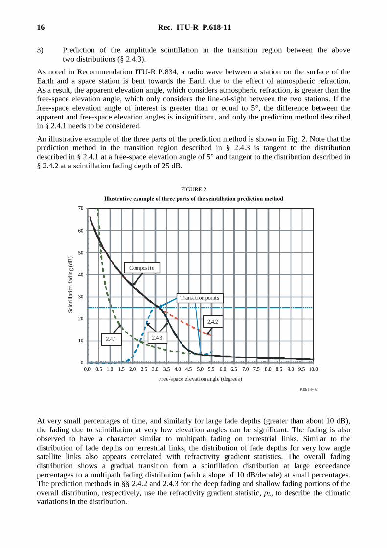
An illustrative example of the three parts of the prediction method is shown in Fig. 2. Note that the
prediction method in the transition region described in § 2.4.3 is tangent to the distribution
described in § 2.4.1 at a free-space elevation angle of 5° and tangent to the distribution described in
§ 2.4.2 at a scintillation fading depth of 25 dB.
FIGURE 2
Illustrative example of three parts of the scintillation prediction method
P.0618-02
0
10
20
30
40
50
60
70
0.0 0.5 1.0 1.5 2.0 2.5 3.0 3.5 4.0 4.5 5.0 5.5 6.0 6.5 7.0 7.5 8.0 8.5 9.0 9.5 10.0
Free-Space Elevation Angle (deg)
0
10
20
30
40
50
60
70
0.0 0.5 1.0 1.5 2.0 2.5 3.0 3.5 4.0 4.5 5.0 5.5 6.0 6.5 7.0 7.5 8.0 8.5 9.0 9.5 10.0
Free-space elevation angle (degrees)
Transition points
Composite
2.4.2
2.4.1 2.4.3
Sci
nti
llat
ion
fad
ing
(dB
)
At very small percentages of time, and similarly for large fade depths (greater than about 10 dB),
the fading due to scintillation at very low elevation angles can be significant. The fading is also
observed to have a character similar to multipath fading on terrestrial links. Similar to the
distribution of fade depths on terrestrial links, the distribution of fade depths for very low angle
satellite links also appears correlated with refractivity gradient statistics. The overall fading
distribution shows a gradual transition from a scintillation distribution at large exceedance
percentages to a multipath fading distribution (with a slope of 10 dB/decade) at small percentages.
The prediction methods in §§ 2.4.2 and 2.4.3 for the deep fading and shallow fading portions of the
overall distribution, respectively, use the refractivity gradient statistic, pL, to describe the climatic
variations in the distribution.
Rec. ITU-R P.618-11 17
The net fade distribution due to tropospheric refractive effects, A( p), is the combination of beam
spreading, scintillation, and multipath-fading effects described above. Tropospheric and ionospheric
scintillation distributions may be combined by summing the respective time percentages that
specified fade levels are exceeded.
2.4.1 Calculation of monthly and long-term statistics of amplitude scintillations at elevation
angles greater than 5°
A general technique for predicting the cumulative distribution of tropospheric scintillation
at elevation angles greater than or equal to 5° is given below. It is based on monthly or longer
averages of temperature and relative humidity, and reflects the specific climatic conditions of the
site. Since the average surface temperature and average surface relative humidity vary with season,
the scintillation fade depth distribution varies with season. The seasonal variation may be predicted
by using seasonal average surface temperature and seasonal average surface relative humidity.
This information may be obtained from weather information for the site of interest.
While the procedure has been tested at frequencies between 7 and 14 GHz, it is recommended for
applications up to at least 20 GHz.
The parameters required for the method are:
t : average surface ambient temperature (°C) at the site for a period of one month
or longer
H : average surface relative humidity (%) at the site for a period of one month or
longer
(NOTE 1 – If no experimental data are available for t and H, the maps of Nwet
in Recommendation ITU-R P.453 may be used.)
f : frequency (GHz), where 4 GHz f 20 GHz
: free-space elevation angle, where 5°
D : physical diameter (m) of the earth-station antenna
: antenna efficiency; if unknown, = 0.5 is a conservative estimate.
If the median value of the wet term of the surface refractivity exceeded for the average year, Nwet,
is obtained from the digital maps in Recommendation ITU-R P.453, go directly to Step 3.
Step 1: For the value of t, calculate the saturation water vapour pressure, es, (hPa), as specified in
Recommendation ITU-R P.453.
Step 2: Compute the wet term of the radio refractivity, Nwet, corresponding to es, t and H as given in
Recommendation ITU-R P.453.
Step 3: Calculate the standard deviation of the reference signal amplitude, ref,:
dB10106.3 4–3–wetref N (35)
Step 4: Calculate the effective path length L:
m
sin1035.2sin
2
4–2
Lh
L (36)
where hL, the height of the turbulent layer, is 1 000 m.
18 Rec. ITU-R P.618-11
Step 5: Estimate the effective antenna diameter, Deff, from the geometrical diameter, D, and the
antenna efficiency :
mDDeff (37)
Step 6: Calculate the antenna averaging factor:
2 11/12 1 5/611 1( ) 3.86 ( 1) sin tan 7.08
6g x x x
x
(38)
where:
)/(22.1 2 LfDxeff
(38a)
If the argument of the square root is negative (i.e. when x 7.0), the predicted scintillation fade
depth for any time percentage is zero and the following steps are not required.
Step 7: Calculate the standard deviation of the signal for the applicable period and propagation
path:
2.1
12/7
)(sin
)(
xgfref (39)
Step 8: Calculate the time percentage factor, a( p), for the time percentage, p, in the range between
0.01% < p 50%:
a( p) = –0.061 (log10 p)3 + 0.072 (log10 p)2 – 1.71 log10 p + 3.0 (40)
Step 9: Calculate the fade depth, A(p), exceeded for p% of the time:
A( p) = a( p) · dB (41)
2.4.2 Calculation of the deep fading part of the scintillation/multipath fading distribution of
elevation angles less than 5°
This method estimates the fade depth for fades greater than or equal to 25 dB due to the
combination of beam spreading, scintillation and multipath fading in the average year and average
annual worst-month. The step-by-step procedure is as follows:
Step 1: Calculate the apparent boresight elevation angle (mrad) corresponding to the desired
free-space elevation angle 0 (mrad) accounting for the effects of refraction for the path of interest
using the method described in § 4 of Recommendation ITU-R P.834.
Step 2: For the path of interest, calculate the geoclimatic factor, Kw, for the average annual worst
month:
105.10
10
LatCC
Lw pK
(42)
where pL (%) is the percentage of time that the refractivity gradient in the lowest 100 m of the
atmosphere is less than –100 N units/km in that month having the highest value of pL from the four
seasonally representative months of February, May, August and November for which maps are
given in Figures 8 to 11 of Recommendation ITU-R P.453.
As an exception, only the maps for May and August should be used for latitudes greater than 60° N
or 60° S.
Rec. ITU-R P.618-11 19
Values of the coefficient C0 in equation (42) corresponding to the type of path are summarized in
Table 3. The coefficient CLat vs. latitude (in °N or °S) is given by:
CLat = 0 for || 53° (43)
CLat = –53 + for 53° < || 60° (44)
CLat = 7 for 60° < || (45)
TABLE 3
Values of the coefficient C0 in equation (42) for various types of propagation path
Step 3: Calculate the fade depth, A(p), exceeded for p% of the time at frequency f (GHz), and the
desired apparent elevation angle, (mrad)
a) for the average year:
pfvKpA w 10101010 log10–)θ1(log5.59–log9–log10)( dB (46)
where:
)ψ2cos1.1(log6.5–8.1–7.0
10 v dB (47)
and the positive sign in equation (47) is for latitudes || 45°, and the negative sign is for latitudes
|| > 45°;
or
b) for the average annual worst-month:
10 10 10 10( ) 10log 9log – 55log (1 θ) –10logwA p K f p dB (48)
Equations (46), (47) and (48) are valid for A(p) greater than or equal to 25 dB. These equations
were developed from data in the frequency range 6-38 GHz and elevation angles in the range from
1° to 4°. They are expected to be valid at least in the frequency range from 1 to 45 GHz and
elevation angles in the range from 0.5° to 5°.
Type of path C0
Propagation paths entirely over land for which the earth-station antenna is less than 700 m
above mean sea level 76
Propagation paths for which the earth-station antenna is higher than 700 m above mean sea
level 70
Propagation paths entirely or partially over water or coastal areas beside such bodies of
water (see(1) for definition of propagation path, coastal areas, and definition of r) 76 + 6r
(1) The variable r in the expression for C0 is the fraction of the propagation path that crosses a body of
water or adjacent coastal areas. Propagation paths passing over a small lake or river are classed as
being entirely over land. Although such bodies of water could be included in the calculation of r, this
yields negligible increases in the value of the coefficient C0 from the overland non-coastal values.
20 Rec. ITU-R P.618-11
2.4.3 Calculation of the shallow fading part of the scintillation/multipath fading distribution
at elevation angles less than 5°
The shallow fading model in this section is developed for scintillation fading in the transition region
for fading less than 25 dB and free-space elevation angles less than 5°.
Step 1: Set A1 = 25 dB and calculate the apparent elevation angle, 1, at the desired time
percentage, p(%), and frequency, f (GHz):
percentage, (%), and frequency, (GHz):
1
1
1
5.50.9
10
1 1
5.950.910
10
1 worst month
10
101 average year
10
w
A
w
A
K f
p
K f
p
mrad (49)
where the geoclimatic factor, wK , is defined in equation (42), and is defined in equation (48).
Step 2: Calculate '1A
yearaverage log1
5.59
month worst log1
55
101
101'
1
e
e
A dB/mrad (50)
Step 3: Calculate 2A from equation (41) of § 2.4.1
2 sA A p dB (51)
at a free-space elevation angle, , of 5°.
Step 4: Calculate '2A as follows:
'2 2
'( ) 1.2 1
( ) tan( ) 1000
g x dxA A
g x d
dB/mrad (52)
where:
1 112 26 12
1 5 112 26 6 12
1770 1 2123 1 cos sin'( )
( )12 1 354 193 1 sin
x x x xg x
g xx x x x
(53a)
2
2 4
1.22 sin1 cos
2 sin 2.35 10
eff
L
D fdx
d h
(53b)
and
Rec. ITU-R P.618-11 21
111 1tan
6 x
(53c)
at a free-space elevation angle, , of 5°, where x, Deff and hL are defined in § 2.4.1.
Step 5: Calculate the apparent elevation angle, 2, corresponding to a free-space elevation angle of
5° using equation (12) of Recommendation ITU-R P.834, and convert 2 to mrad.
Step 6: Calculate the scintillation fading, A(p), exceeded for p (%) of the time at the desired
apparent elevation angle, (mrad), by interpolating between the points 111 ,,θ AA and 222 ,,θ AA
using the following cubic exponential model:
2 2
1 1 1 1 2( ) expA p A p p p
(54)
where:
1
'
1)(αA
Ap
2
1
2
δ
αδ–ln
)(β
A
A
p
'2 2
22
– (α 2βδ)γ( )
δ
A Ap
A
12 θ–θδ
The fade depth, A(p), is applicable for apparent elevation angles in the transition region;
i.e. for 21 θθθ , and %500 p .
2.5 Estimation of total attenuation due to multiple sources of simultaneously occurring
atmospheric attenuation
For systems operating at frequencies above about 18 GHz, and especially those operating with low
elevation angles and/or margins, the effect of multiple sources of simultaneously occurring
atmospheric attenuation must be considered.
Total attenuation (dB) represents the combined effect of rain, gas, clouds and scintillation and
requires one or more of the following input parameters:
AR ( p) : attenuation due to rain for a fixed probability (dB), as estimated by Ap in
equation (8)
AC ( p) : attenuation due to clouds for a fixed probability (dB), as estimated by
Recommendation ITU-R P.840
AG ( p) : gaseous attenuation due to water vapour and oxygen for a fixed probability (dB), as
estimated by Recommendation ITU-R P.676
AS ( p) : attenuation due to tropospheric scintillation for a fixed probability (dB), as estimated
by equation (41)
where p is the probability of the attenuation being exceeded in the range 50% to 0.001%.
Gaseous attenuation as a function of percentage of time can be calculated using § 2.2 of Annex 2 of
Recommendation ITU-R P.676 if local meteorological data at the required time percentage are
22 Rec. ITU-R P.618-11
available. In the absence of local data at the required time percentage, the mean gaseous attenuation
should be calculated and used in equation (55).
A general method for calculating total attenuation for a given probability, AT ( p), is given by:
)()()()()( 22pApApApApA SCRGT (55)
where:
AC ( p) = AC (1%) for p < 1.0% (56)
AG ( p) = AG (1%) for p < 1.0% (57)
Equations (56) and (57) take account of the fact that a large part of the cloud attenuation and
gaseous attenuation is already included in the rain attenuation prediction for time percentages
below 1%.
When the complete prediction method above was tested using the procedure set out in Annex 1 to
Recommendation ITU-R P.311, the results were found to be in good agreement with available
measurement data for all latitudes and in the probability range 0.001% to 1%, with an overall r.m.s.
error of about 35%, when used with the contour rain maps in Recommendation ITU-R P.837. When
tested against multi-year Earth-space data, the overall r.m.s. error was found to be about 25%. Due
to the dominance of different effects at different probabilities as well as the inconsistent availability
of test data at different probability levels, some variation of r.m.s. error occurs across the
distribution of probabilities.
2.6 Attenuation by sand and dust storms
Very little is known about the effects of sand and dust storms on radio signals on slant-paths.
Available data indicate that at frequencies below 30 GHz, high particle concentrations and/or high
moisture contents are required to produce significant propagation effects.
3 Noise temperature
As attenuation increases, so does emission noise. For earth stations with low-noise front-ends, this
increase of noise temperature may have a greater impact on the resulting signal-to-noise ratio than
the attenuation itself.
The atmospheric contribution to antenna noise in a ground station may be estimated with the
equation:
Ts = Tm (1 – 10–A/10) (58)
where:
Ts : sky-noise temperature (K) as seen by the antenna
A : path attenuation (dB)
Tm : effective temperature (K) of the medium.
The effective temperature is dependent on the contribution of scattering to attenuation and on the
physical extent of clouds and rain cells on the vertical variation of the physical temperature of the
scatterers and, to a lesser extent, on the antenna beamwidth. By comparing radiometric observations
and simultaneous beacon attenuation measurements, the effective temperature of the medium has
been determined to lie in the range 260-280 K for rain and clouds along the path at frequencies
between 10 and 30 GHz.
Rec. ITU-R P.618-11 23
When the attenuation is known, the following effective temperatures of the mediums may be used
to obtain an upper limit to sky-noise temperature at frequencies below 60 GHz:
Tm = 280 K for clouds
Tm = 260 K for rain
The noise environments of stations on the surface of the Earth and in space are treated in detail in
Recommendation ITU-R P.372.
For satellite telecommunication systems using the geostationary orbit, earth stations will find that
the Sun and, to a lesser extent, the Moon, are significant noise sources at all frequencies and that the
galactic background is a possibly significant consideration at frequencies below about 2 GHz (see
Recommendation ITU-R P.372). In addition, contributions to the sky background noise temperature
may be given by Cygnus A and X, Cassiopeia A, Taurus and the Crab nebula.
To determine the system noise temperature of earth stations from the brightness temperatures
discussed above, the equations of Recommendation ITU-R P.372 may be used.
4 Cross-polarization effects
Frequency reuse by means of orthogonal polarizations is often used to increase the capacity of
space telecommunication systems. This technique is restricted, however, by depolarization on
atmospheric propagation paths. Various depolarization mechanisms, especially hydrometeor effects,
are important in the troposphere.
Faraday rotation of the plane of polarization by the ionosphere is discussed in Recommendation
ITU-R P.531. As much as 1° of rotation may be encountered at 10 GHz, and greater rotations at
lower frequencies. As seen from the earth station, the planes of polarization rotate in the same
direction on the up- and down-links. It is therefore not possible to compensate for Faraday rotation
by rotating the feed system of the antenna, if the same antenna is used both for transmitting and
receiving.
4.1 Calculation of long-term statistics of hydrometeor-induced cross-polarization
To calculate long-term statistics of depolarization from rain attenuation statistics the following
parameters are needed:
Ap : rain attenuation (dB) exceeded for the required percentage of time, p, for the
path in question, commonly called co-polar attenuation (CPA)
: tilt angle of the linearly polarized electric field vector with respect to the
horizontal (for circular polarization use = 45°)
f : frequency (GHz)
: path elevation angle (degrees).
The method described below to calculate cross-polarization discrimination (XPD) statistics from
rain attenuation statistics for the same path is valid for 6 f 55 GHz and 60°. The procedure
for scaling to frequencies down to 4 GHz is given in § 4.3 (and see Step 8 below).
Step 1: Calculate the frequency-dependent term:
GHz5536311 log935
GHz36914log26
GHz96328log60
f.f.
f.f
f.f
C f (59)
24 Rec. ITU-R P.618-11
Step 2: Calculate the rain attenuation dependent term:
CA = V ( f ) log Ap (60)
where:
GHz55400.13
GHz40206.22
GHz2098.12
GHz968.30
15.0
19.0
21.0
ff
f
ff
ff
fV
Step 3: Calculate the polarization improvement factor:
C = –10 log [1 – 0.484 (1 + cos 4)] (61)
The improvement factor C = 0 for = 45° and reaches a maximum value of 15 dB for = 0°
or 90°.
Step 4: Calculate the elevation angle-dependent term:
C = –40 log (cos ) for 60° (62)
Step 5: Calculate the canting angle dependent term:
C = 0.0053 2 (63)
is the effective standard deviation of the raindrop canting angle distribution, expressed in degrees;
takes the value 0°, 5°, 10° and 15° for 1%, 0.1%, 0.01% and 0.001% of the time, respectively.
Step 6: Calculate rain XPD not exceeded for p% of the time:
XPDrain = Cf – CA + C + C + C dB (64)
Step 7: Calculate the ice crystal dependent term:
Cice = XPDrain (0.3 + 0.1 log p)/2 dB (65)
Step 8: Calculate the XPD not exceeded for p% of the time, including the effects of ice:
XPDp = XPDrain – Cice dB (66)
In this prediction method in the frequency band 4 to 6 GHz where path attenuation is low,
Ap statistics are not very useful for predicting XPD statistics. For frequencies below 6 GHz,
the frequency-scaling formula of § 4.3 can be used to scale cross-polarization statistics calculated
for 6 GHz to a lower frequency between 4 and 6 GHz.
4.2 Joint statistics of XPD and attenuation
The conditional probability distribution of XPD for a given value of attenuation, Ap, can be
modelled by assuming that the cross-polar to co-polar voltage ratio, r = 10–XPD/20, is normally
distributed. Parameters of the distribution are the mean value, rm, which is very close to 10–XPDrain
/20,
with XPDrain given by equation (64), and the standard deviation, r, which assumes the almost-
constant value of 0.038 for 3 dB Ap 8 dB.
Rec. ITU-R P.618-11 25
4.3 Long-term frequency and polarization scaling of statistics of hydrometeor-induced
cross-polarization
Long-term XPD statistics obtained at one frequency and polarization tilt angle can be scaled to
another frequency and polarization tilt angle using the semi-empirical formula:
GHz30,4for
)4cos1(484.0–1
)4cos1(484.0–1log20– 21
11
2212 ff
f
fXPDXPD (67)
where XPD1 and XPD2 are the XPD values not exceeded for the same percentage of time at
frequencies f1 and f2 and polarization tilt angles, 1 and 2, respectively.
Equation (67) is based on the same theoretical formulation as the prediction method of § 4.1, and
can be used to scale XPD data that include the effects of both rain and ice depolarization, since it
has been observed that both phenomena have approximately the same frequency dependence at
frequencies less than about 30 GHz.
4.4 Data relevant to cross-polarization cancellation
Experiments have shown that a strong correlation exists between rain depolarization at 6 and 4 GHz
on Earth-space paths, both on the long term and on an event basis, and uplink depolarization
compensation utilizing concurrent down-link depolarization measurements appears feasible. Only
differential phase effects were apparent, even for severe rain events, and single-parameter
compensation (i.e. for differential phase) appears sufficient at 6 and 4 GHz.
Measurements at 6 and 4 GHz have also shown that 99% of the XPD variations are slower than
4 dB/s, or equivalently, less than 1.5°/s in the mean path differential phase shift. Therefore, the
time constant of a depolarization compensation system at these frequencies need only be about 1 s.
5 Propagation delays
Radiometeorologically-based methods for estimating the average propagation delay or range error,
and the corresponding variations, for Earth-space paths through the troposphere are available in
Recommendation ITU-R P.834. The delay variance is required for satellite ranging and
synchronization in digital satellite communication systems. At frequencies above 10 GHz, the
ionospheric time delay (see Recommendation ITU-R P.531) is generally smaller than that for the
troposphere, but may have to be considered in special cases.
Range determination to centimetre accuracy requires careful consideration of the various
contributions to excess range delay. The water vapour component amounts to 10 cm for a zenith
path and a reference atmosphere with surface water vapour concentration of 7.5 g/m3 and 2 km
scale height (see Recommendation ITU-R P.676). This contribution is the largest source of
uncertainty, even though the dry atmosphere adds 2.3 m of the zenithal excess range delay.
For current satellite telecommunication applications, additional propagation delays contributed by
precipitation are sufficiently small to be ignored.
6 Bandwidth limitations
In the vicinity of the absorption lines of atmospheric gases, anomalous dispersion produces small
changes in the refractive index. However, these refractive index changes are small in the bands
allocated to Earth-space communications, and will not restrict the bandwidth of systems.
Multiple scattering in rain can limit the bandwidth of incoherent transmission systems due to
variation in time delays of the multiple-scattered signals; however, the attenuation itself under such
26 Rec. ITU-R P.618-11
circumstances will present a far more serious problem. A study of the problem of bandwidth
limitations imposed by the frequency dependence of attenuation and phase shift due to rain on
coherent transmission systems showed that such bandwidth limitations are in excess of 3.5 GHz for
all situations likely to be encountered. These are greater than any bandwidth allocated for
Earth-space communications below 40 GHz, and the rain attenuation will therefore be far more
important than its frequency dependence.
7 Angle of arrival
Elevation-angle errors due to refraction are discussed in Recommendation ITU-R P.834. The total
angular refraction (the increase in apparent elevation) is about 0.65°, 0.35° and 0.25°, for elevation
angles of 1°, 3° and 5°, respectively, for a tropical maritime atmosphere. For a polar continental
climate the corresponding values are 0.44°, 0.25° and 0.17°. Other climates will have values
between these two extremes. The day-to-day variation in apparent elevation is of the order of
0.1° (r.m.s.) at 1° elevation, but the variation decreases rapidly with increasing elevation angle.
Short-term angle-of-arrival fluctuations are discussed in Recommendation ITU-R P.834. Short-term
variations, due to changes in the refractivity-height variation, may be of the order of 0.02° (r.m.s.)
at 1° elevation, again decreasing rapidly with increasing elevation angle. In practice, it is difficult to
distinguish between the effect of the short-term changes in the refractivity-height distribution and the
effect of random irregularities superimposed on that distribution. A statistical analysis of the short-
term angle-of-arrival fluctuation at 19.5 GHz and at an elevation angle of 48° suggests that both in
elevation and azimuth directions, standard deviations of angle-of-arrival fluctuations are about 0.002°
at the cumulative time percentage of 1%. The seasonal variation of angle-of-arrival fluctuations
suggests that the fluctuations increase in summer and decrease in winter. The diurnal variation
suggests that they increase in the daytime and decrease both in the early morning and the evening.
8 Calculation of long-term statistics for non-GSO paths
The prediction methods described above were derived for applications where the elevation angle
remains constant. For non-GSO systems, where the elevation angle is varying, the link availability
for a single satellite can be calculated in the following way:
a) calculate the minimum and maximum elevation angles at which the system will be expected
to operate;
b) divide the operational range of angles into small increments (e.g. 5° wide);
c) calculate the percentage of time that the satellite is visible as a function of elevation angle
in each increment;
d) for a given propagation impairment level, find the time percentage that the level is
exceeded for each elevation angle increment;
e) for each elevation angle increment, multiply the results of c) and d) and divide by 100,
giving the time percentage that the impairment level is exceeded at this elevation angle;
f) sum the time percentage values obtained in e) to arrive at the total system time percentage
that the impairment level is exceeded.
In the case of multi-visibility satellite constellations employing satellite path diversity
(i.e. switching to the least impaired path), an approximate calculation can be made assuming that
the spacecraft with the highest elevation angle is being used.