Proofs of the Theorems of Plastic Analysis

and Design

Aamer Haque

Abstract

The proofs of the theorems of plastic analysis and design are provided in Horne [9], Neal [11]. These proofs are reproducedwith additional details, explanations, and examples.

Preprint

Preprint submitted to Elsevier April 23, 2015

1. Plastic Analysis

1.1. Formulation

1.1.1. Introduction

Applied loads Wj = αjW j = 1, . . . , Nloads

Moment capacities Mkp = βkMp k = 1, . . . , Nmembers

Moment distributions mi i = 1, . . . , N

Table 1: Notation for plastic analysis

The purpose of plastic analysis is to compute the collapseload of a structure. In other words, we wish to determine thevalue of applied loads which produce a mechanism of collapse.A mechanism is produced when a sufficient number of plas-tic hinges occur such that certain deflections of the structureincrease without requiring an increase of the applied loads.These concepts and a full description of plastic analysis areprovided in many texts on plastic analysis: Baker and Hey-man [1], Beedle [2], Heyman [7], Hodge [8], Horne [9], Neal[11]. Plastic analysis is a 1st order analysis method. The ap-plied loads are assumed to act on the undeformed structure;p-∆ and p-δ effects are ignored. Also, Hooke’s law is assumedto hold in the elastic regions of a structure. The structuralmaterials are described by an ideal elastic-plastic constitutiverelation. This paper will only consider indeterminate frameswith a finite number of applied point loads.

In order to provide a general description of problems inplastic analysis, several items of notation are required. Theapplied loads are denoted as Wj where j = 1, . . . , Nloads. Allloads are assumed to act simultaneously. Proportional loadingis assumed. This means that every load is a scaled factor of asingle positive load W . Each member of the frame has plas-tic bending moment capacity Mk

p where k = 1, . . . , Nmembers.Members must be able to form a plastic hinge when the max-imum absolute bending moment reaches Mk

p . They must alsobe designed to resist failure due to buckling and other insta-bilities at their plastic moment capacity. It is always possibleto represent the plastic moment capacities as a scaled factorof a single value Mp which is chosen for convenience. Plastichinges can only form at the locations of applied point loadsand at joints (i.e. connections between members). The mo-ments at these locations are denoted mi where i = 1, . . . , N .The moments mi may be elastic or plastic. Since we assumedall applied loads are point loads, the bending moments willvary linearly between the locations of mi. By the above defi-nitions, we clearly have N ≥ Nloads and N ≥ Nmembers. Table1 summarizes the notation used in plastic analysis.

It should be noted that in elastic analysis, multiplying theapplied loads by a load factor λ results in bending momentsbeing multiplied by the same factor: λW ⇒ λmi. This prin-ciple is not valid in plastic analysis. The reason is that asplastic hinges are formed, the moment remains fixed at theplastic hinges and the nature of the structure is altered. Thenumber of redundancies is reduced by one for each plastichinge.

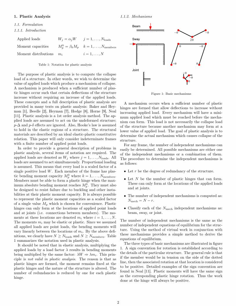
1.1.2. Mechanisms

Figure 1: Basic mechanisms

A mechanism occurs when a sufficient number of plastichinges are formed that allow deflections to increase withoutincreasing applied load. Every mechanism will have a mini-mum applied load which must be reached before the mecha-nism can form. This load is not necessarily the collapse loadof the structure because another mechanism may form at alower value of applied load. The goal of plastic analysis is todetermine the actual mechanism which causes collapse of thestructure.

For any frame, the number of independent mechanisms caneasily be determined. All possible mechanisms are either oneof the independent mechanisms or a combination of them.The procedure to determine the independent mechanisms isas follows:

• Let r be the degree of redundancy of the structure.

• Let N be the number of plastic hinges that can form.These can only form at the locations of the applied loadsand at joints.

• The number of independent mechanisms is computed as:Nmech = N − r.

• Classify each of the Nmech independent mechanisms as:beam, sway, or joint.

The number of independent mechanisms is the same as thenumber of independent equations of equilibrium for the struc-ture. Using the method of virtual work in conjunction withthese mechanisms provides a simple method to derive theequations of equilibrium.

The three types of basic mechanisms are illustrated in figure1. A sign convention for rotation is established according tothe details of the particular structure. The general rule is thatif the member would be in tension on the side of the dottedline, then the associated rotation at that location is consideredto be positive. Detailed examples of the sign convention arefound in Neal [11]. Plastic moments will have the same signas the corresponding plastic hinge rotation. Thus the workdone at the hinge will always be positive.

2

1.1.3. Theorems

No restrictions have yet been placed on the distribution ofbending moments. We first restrict the bending moments tosatisfy the equations of equilibrium.

Definition 1.1. The bending moments mi of a frame arestatically admissible if they satisfy the equations of equilib-rium with the applied loads Wj .

The equations of equilibrium for mi can be formulated us-ing the method of virtual work. For an indeterminate struc-ture, there may be an infinite number of admissible bendingmoments for a structure. The actual bending moments arecomputed by performing a complete elastic-plastic analysis.

We also must ensure that the bending moments do no ex-ceed the plastic moment capacities of the corresponding mem-bers. We require a map K : {1, . . . , N} → {1, . . . , Nmembers}from the location of the moment mi to its corresponding mem-ber k. Thus k = K(i) is the index of the member whichcontains the bending moment mi.

Definition 1.2. The bending moments mi of a frame aresafe if they do not exceed their corresponding plastic momentcapacities.

|mi| ≤ MK(i)p , i = 1, . . . , N

Recalling that all applied loads are proportional to the rep-resentative load W , we can state the goal of plastic analysisin terms of this load.

Definition 1.3. The smallest load W which causes the frameto form a mechanism is called the collapse load Wc.

We shall frequently require the Principle of Virtual Workfor beams in the form of virtual displacements.

Definition 1.4. The Principle of Virtual Work states thatexternal virtual work equals internal virtual work.

Nloads∑

j=1

Wj δ∆j =N∑

i=1

mi δθi +

Nmembers∑

k=1

ˆ Lk

0

m(x) δκ(x) dx

where δ∆j are the virtual displacements associated with Wj ,δθi are the virtual rotations at mi, and δκ(x) is the virtualcurvature in member k which has length Lk.

The Principle of Complementary Virtual Work for beamswill also be needed.

Definition 1.5. The Principle of Complementary VirtualWork states that the external complementary work equalsthe internal complementary work.

Nloads∑

j=1

δWj ∆j =

N∑

i=1

δmi θi +

Nmembers∑

k=1

ˆ Lk

0

δm(x)κ(x) dx

where δWj are the virtual forces associated with ∆j , δmi

are the virtual moments for θi, and δm(x) is the virtual mo-ment in member k which has length Lk. The virtual momentsδm(x) and δmi must be in equilibrium with the virtual forcesδWj .

Theorem 1.1 (Static or Lower Bound Theorem). If a set ofloads on a frame produces bending moments which are stati-cally admissible and safe, then the loads are less than or equalto the collapse load.

W ≤ Wc

Proof. Define the load factor λc > 0 such that Wc = λcW .Consider the actual work done during the collapse mechanismundergoing small real displacements:

λc

Nloads∑

j=1

Wj ∆j =

N∑

i=1

M ip θ̂i (1.1)

∆j is the displacement in the direction of Wj ,∣

∣M ip

∣

∣ = MK(i)p

is the plastic moment at location i, and θ̂i is the plastic hingerotation at location i. Note that we set θ̂i = 0 at locationswhich are not plastic hinges. The right hand side of equation(1.1) is positive since the plastic moment and plastic hingerotation have the same sign and produce positive work. Thusthe sum on the left hand side is positive even though everyterm may not be positive.

Now consider ∆j and θ̂i as virtual displacements for virtualwork computed for the statically admissible and safe load W :

Nloads∑

j=1

Wj ∆j =N∑

i=1

mi θ̂i (1.2)

Subtracting (1.2) from (1.1) we obtain:

(λc − 1)

Nloads∑

j=1

Wj ∆j =N∑

i=1

(

M ip −mi

)

θ̂i (1.3)

A safe distribution of bending moments implies:

−∣

∣M ip

∣

∣ ≤ mi ≤∣

∣M ip

∣

∣

Thus every term on the right hand side of (1.3) is non-negative. Since the sum on the left hand side is positive,we have λc − 1 ≥ 0. λc ≥ 1 ⇒ Wc ≥ W and the theorem isproved.

Corollary 1.1. Increasing the strength of any members in aframe cannot decrease the collapse load.

Proof. Let λc1 be the original collapse load factor for stat-

ically admissible and safe load W . Then λc1 |mi| ≤ MK(i)p1

for i = 1, . . . , N . For the new frame we have the followingrelations:

Mkp1 = Mk

p2 if member k is not strengthened

Mkp1 < Mk

p2 if member k is strengthened

λc1 |mi| ≤ MK(i)p1 ≤ M

K(i)p2

This means that λc1W is statically admissible and safe for thenew frame. By the Lower Bound Theorem: λc1W ≤ λc2W ⇒λc1 ≤ λc2.

3

Theorem 1.2 (Kinematic or Upper Bound Theorem). If aset of loads on a frame produces a mechanism, then the loadsare greater than or equal to the collapse load.

Wc ≤ W

Proof. Consider an arbitrary mechanism with associated loadW . Compute the actual work associated with this mechanism:

Nloads∑

j=1

Wj ∆j =

N∑

i=1

M ip θ̂i (1.4)

where all quantities are defined the same as in the proof ofthe Lower Bound Theorem. Both sides of equation (1.4) arepositive.

Let mi be the distribution of bending moments for the col-lapse load. These moments satisfy the equations of equilib-rium with the collapse load λcW . Considering the displace-ments in (1.4) to be virtual and computing the virtual workfor the collapse load we have:

λc

Nloads∑

j=1

Wj ∆j =N∑

i=1

mi θ̂i (1.5)

By subtracting (1.5) from (1.4) we get:

(1− λc)

Nloads∑

j=1

Wj ∆j =

N∑

i=1

(

M ip −mi

)

θ̂i (1.6)

The distribution of bending moments at collapse satisfies:

−∣

∣M ip

∣

∣ ≤ mi ≤∣

∣M ip

∣

∣

Every term on the right hand side of (1.6) is non-negative.Since the sum on the left hand side is positive, we have 1−λc ≥0. λc ≤ 1 ⇒ Wc ≤ W and the theorem is proved.

Corollary 1.2. Decreasing the strength of any members in aframe cannot increase the collapse load.

Proof. Let λc1 be the original collapse load factor for stati-cally admissible and safe load W . The Upper Bound Theoremstates that the collapse mechanism of the original frame pro-vides λc1W as an upper bound for the new frame. Henceλc2W ≤ λc1W ⇒ λc2 ≤ λc1 and the corollary is proved.

Theorem 1.3 (Uniqueness Theorem). Suppose a set of loadson a frame produces bending moments which are staticallyadmissible, safe, and results in a mechanism. Then the loadsequal the collapse load.

Proof. We have Wc ≤ W by the Upper Bound Theorem andW ≤ Wc by the Lower Bound Theorem. Then Wc ≤ W ≤ Wc

implies W = Wc.

Henceforth we shall assume that we can find a set of loadswhich satisfies the Uniqueness Theorem. Thus we can com-pute the collapse load.

The Lower Bound Theorem states that every load Ws whichresults in a statically admissible and safe distribution of bend-ing moments is a lower bound for the collapse load. If S isthe set of all safe and statically admissible loads, then the

Uniqueness Theorem implies the largest such load would bethe collapse load:

Wc = maxs∈S

Ws

Unfortunately, the set S is infinite and thus it is difficult tocompute Wc in this way.

The Upper Bound Theorem implies that every load thatresults in a mechanism is an upper bound for the collapseload. Using the Uniqueness Theorem we can state that thesmallest such load is the collapse load:

Wc = minm∈M

Wm

Since the set of mechanisms M is finite, it is possible to com-pute all such loads and choose the smallest one. This pro-cedure becomes very cumbersome for structures with a largenumber of possible mechanisms.

It can be shown that the bending moment distributions andcurvature of members remain constant during plastic collapse.

Theorem 1.4. The bending moments and curvature remainconstant during plastic collapse.

Proof. The Uniqueness Theorem implies that at the momentof collapse, the applied loads are in equilibrium with the mo-ments. Let the moments increase by increments δmi at theplastic hinges and δm(x) elsewhere. The corresponding dis-placements increase by increments δθi and δκ(x). The appliedloads remain constant during collapse and thus δWj = 0. Wecan use the Principle of Virtual Work by choosing the mo-ment increments to be real and the displacement incrementsas virtual. Similarly using the Principle of ComplementaryVirtual Work we can consider the displacement increments asreal and the moment increments as virtual. Either of theseprinciples results in the following equation:

N∑

i=1

δmi δθi +

Nmembers∑

k=1

ˆ Lk

0

δm(x) δκ(x) dx = 0

The values of terms in the first sum depend on whether thereis a plastic hinge at location i:

i is a plastic hinge ⇒ δmi = 0

i is not a plastic hinge ⇒ δθi = 0

Thus the first sum is zero. We are left with the second term:

Nmembers∑

k=1

ˆ Lk

0

δm(x) δκ(x) dx = 0

We note that δm(x) δκ(x) ≥ 0 because the moment and curva-ture increments have the same sign. If κ(x) is virtual, then itis arbitrary and we must have δm(x) = 0 everywhere. On theother hand if δm(x) is virtual and arbitrary, then δκ(x) = 0everywhere. Thus the moments and curvature do not changeduring plastic collapse.

Theorem 1.4 states that the deformation of each memberremains fixed during plastic collapse. The frame subsequentlychanges shape due to rigid body motions only.

4

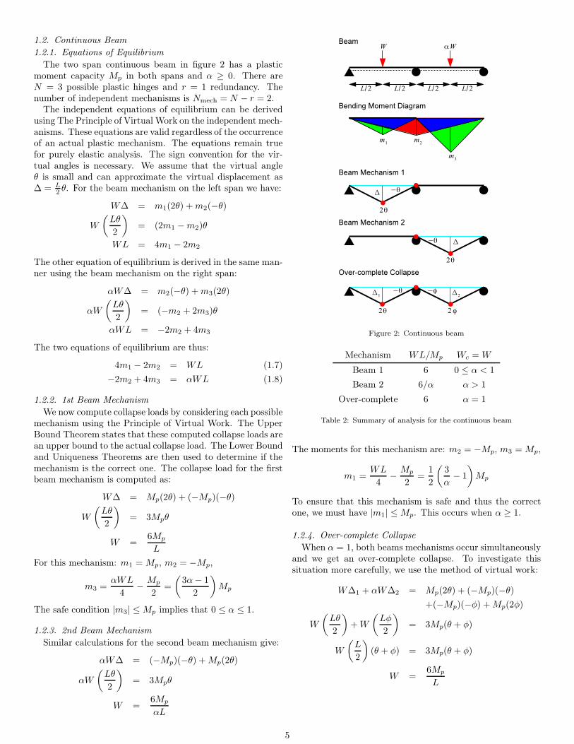
1.2. Continuous Beam

1.2.1. Equations of Equilibrium

The two span continuous beam in figure 2 has a plasticmoment capacity Mp in both spans and α ≥ 0. There areN = 3 possible plastic hinges and r = 1 redundancy. Thenumber of independent mechanisms is Nmech = N − r = 2.

The independent equations of equilibrium can be derivedusing The Principle of Virtual Work on the independent mech-anisms. These equations are valid regardless of the occurrenceof an actual plastic mechanism. The equations remain truefor purely elastic analysis. The sign convention for the vir-tual angles is necessary. We assume that the virtual angleθ is small and can approximate the virtual displacement as∆ = L

2 θ. For the beam mechanism on the left span we have:

W∆ = m1(2θ) +m2(−θ)

W

(

Lθ

2

)

= (2m1 −m2)θ

WL = 4m1 − 2m2

The other equation of equilibrium is derived in the same man-ner using the beam mechanism on the right span:

αW∆ = m2(−θ) +m3(2θ)

αW

(

Lθ

2

)

= (−m2 + 2m3)θ

αWL = −2m2 + 4m3

The two equations of equilibrium are thus:

4m1 − 2m2 = WL (1.7)

−2m2 + 4m3 = αWL (1.8)

1.2.2. 1st Beam Mechanism

We now compute collapse loads by considering each possiblemechanism using the Principle of Virtual Work. The UpperBound Theorem states that these computed collapse loads arean upper bound to the actual collapse load. The Lower Boundand Uniqueness Theorems are then used to determine if themechanism is the correct one. The collapse load for the firstbeam mechanism is computed as:

W∆ = Mp(2θ) + (−Mp)(−θ)

W

(

Lθ

2

)

= 3Mpθ

W =6Mp

L

For this mechanism: m1 = Mp, m2 = −Mp,

m3 =αWL

4−

Mp

2=

(

3α− 1

2

)

Mp

The safe condition |m3| ≤ Mp implies that 0 ≤ α ≤ 1.

1.2.3. 2nd Beam Mechanism

Similar calculations for the second beam mechanism give:

αW∆ = (−Mp)(−θ) +Mp(2θ)

αW

(

Lθ

2

)

= 3Mpθ

W =6Mp

αL

Figure 2: Continuous beam

Mechanism WL/Mp Wc = W

Beam 1 6 0 ≤ α < 1

Beam 2 6/α α > 1

Over-complete 6 α = 1

Table 2: Summary of analysis for the continuous beam

The moments for this mechanism are: m2 = −Mp, m3 = Mp,

m1 =WL

4−

Mp

2=

1

2

(

3

α− 1

)

Mp

To ensure that this mechanism is safe and thus the correctone, we must have |m1| ≤ Mp. This occurs when α ≥ 1.

1.2.4. Over-complete Collapse

When α = 1, both beams mechanisms occur simultaneouslyand we get an over-complete collapse. To investigate thissituation more carefully, we use the method of virtual work:

W∆1 + αW∆2 = Mp(2θ) + (−Mp)(−θ)

+(−Mp)(−φ) +Mp(2φ)

W

(

Lθ

2

)

+W

(

Lφ

2

)

= 3Mp(θ + φ)

W

(

L

2

)

(θ + φ) = 3Mp(θ + φ)

W =6Mp

L

5

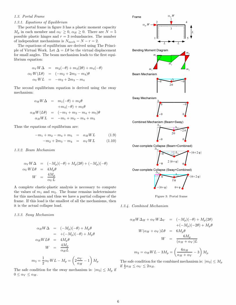
1.3. Portal Frame

1.3.1. Equations of Equilibrium

The portal frame in figure 3 has a plastic moment capacityMp in each member and αV ≥ 0, αH ≥ 0. There are N = 5possible plastic hinges and r = 3 redundancies. The numberof independent mechanisms is Nmech = N − r = 2.

The equations of equilibrium are derived using The Princi-ple of Virtual Work. Let ∆ = Lθ be the virtual displacementfor small angles. The beam mechanism leads to the first equi-librium equation:

αV W∆ = m2(−θ) +m3(2θ) +m4(−θ)

αV W (Lθ) = (−m2 + 2m3 −m4)θ

αV WL = −m2 + 2m3 −m4

The second equilibrium equation is derived using the swaymechanism:

αHW∆ = m1(−θ) +m2θ

+m4(−θ) +m5θ

αHW (Lθ) = (−m1 +m2 −m4 +m5)θ

αHWL = −m1 +m2 −m4 +m5

Thus the equations of equilibrium are:

−m1 +m2 −m4 +m5 = αHWL (1.9)

−m2 + 2m3 −m4 = αV WL (1.10)

1.3.2. Beam Mechanism

αV W∆ = (−Mp)(−θ) +Mp(2θ) + (−Mp)(−θ)

αV WLθ = 4Mpθ

W =4Mp

αV L

A complete elastic-plastic analysis is necessary to computethe values of m1 and m5. The frame remains indeterminatefor this mechanism and thus we have a partial collapse of theframe. If this load is the smallest of all the mechanisms, thenit is the actual collapse load.

1.3.3. Sway Mechanism

αHW∆ = (−Mp)(−θ) +Mpθ

= +(−Mp)(−θ) +Mpθ

αHWLθ = 4Mpθ

W =4Mp

αHL

m3 =1

2αV WL−Mp =

(

2αV

αH

− 1

)

Mp

The safe condition for the sway mechanism is: |m3| ≤ Mp if0 ≤ αV ≤ αH .

Figure 3: Portal frame

1.3.4. Combined Mechanism

αHW∆H + αV W∆V = (−Mp)(−θ) +Mp(2θ)

+(−Mp)(−2θ) +Mpθ

W (αH + αV )Lθ = 6Mpθ

W =6Mp

(αH + αV )L

m2 = αHWL− 3Mp =

(

6αH

αH + αV

− 3

)

Mp

The safe condition for the combined mechanism is: |m2| ≤ Mp

if 12αH ≤ αV ≤ 2αH .

6

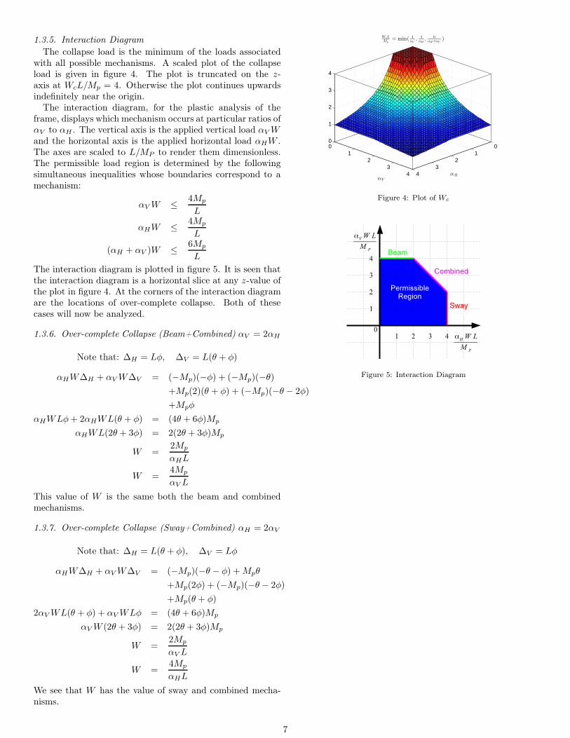
1.3.5. Interaction Diagram

The collapse load is the minimum of the loads associatedwith all possible mechanisms. A scaled plot of the collapseload is given in figure 4. The plot is truncated on the z-axis at WcL/Mp = 4. Otherwise the plot continues upwardsindefinitely near the origin.

The interaction diagram, for the plastic analysis of theframe, displays which mechanism occurs at particular ratios ofαV to αH . The vertical axis is the applied vertical load αV Wand the horizontal axis is the applied horizontal load αHW .The axes are scaled to L/MP to render them dimensionless.The permissible load region is determined by the followingsimultaneous inequalities whose boundaries correspond to amechanism:

αV W ≤4Mp

L

αHW ≤4Mp

L

(αH + αV )W ≤6Mp

L

The interaction diagram is plotted in figure 5. It is seen thatthe interaction diagram is a horizontal slice at any z-value ofthe plot in figure 4. At the corners of the interaction diagramare the locations of over-complete collapse. Both of thesecases will now be analyzed.

1.3.6. Over-complete Collapse (Beam+Combined) αV = 2αH

Note that: ∆H = Lφ, ∆V = L(θ + φ)

αHW∆H + αV W∆V = (−Mp)(−φ) + (−Mp)(−θ)

+Mp(2)(θ + φ) + (−Mp)(−θ − 2φ)

+Mpφ

αHWLφ+ 2αHWL(θ + φ) = (4θ + 6φ)Mp

αHWL(2θ + 3φ) = 2(2θ + 3φ)Mp

W =2Mp

αHL

W =4Mp

αV L

This value of W is the same both the beam and combinedmechanisms.

1.3.7. Over-complete Collapse (Sway+Combined) αH = 2αV

Note that: ∆H = L(θ + φ), ∆V = Lφ

αHW∆H + αV W∆V = (−Mp)(−θ − φ) +Mpθ

+Mp(2φ) + (−Mp)(−θ − 2φ)

+Mp(θ + φ)

2αV WL(θ + φ) + αV WLφ = (4θ + 6φ)Mp

αV W (2θ + 3φ) = 2(2θ + 3φ)Mp

W =2Mp

αV L

W =4Mp

αHL

We see that W has the value of sway and combined mecha-nisms.

01

23

4

01

23

4

0

1

2

3

4

αH

WcLMp

= min( 4αV

, 4αH

, 6αH+αV

)

αV

Figure 4: Plot of Wc

Figure 5: Interaction Diagram

7

2. Minimum Weight Design

2.1. Formulation

2.1.1. Introduction

The general goal of structural design is to choose structuralmembers that can carry the loads applied to the structurewithout failure. The applied loads Wj = αjW and geome-try/topology of the structure are known. Members of suffi-cient moment capacity must be chosen. Plastic design focuseson moment capacities because the required axial capacities ofcolumns are easily computed. After members are chosen inthis manner, they are checked for their ability to resist buck-ling and other instabilities. Members found to be inadequateare then replaced. These issues will not be discussed furtherbut are discussed in texts on structural stability: Chen andAtsuta [3, 4], Chen and Lui [6, 5], McGuire [10]. Furthermore,we shall focus exclusively on planar steel frames even thoughconcrete frames can also be designed using plastic analysis.

It is obvious that many different designs will be adequatefor a given structure. However, we don’t desire any design butone that minimizes total structural weight. The total weightW of a structure is the sum of the weights of its members:

W =

Nmembers∑

k=1

wk Lk

wk is the weight per length of member k and Lk is the lengthof member k.

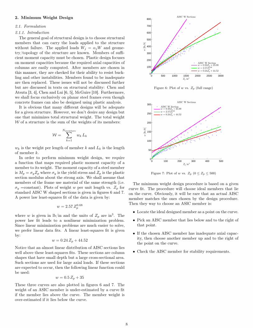
In order to perform minimum weight design, we requirea function that maps required plastic moment capacity of amember to its weight. The moment capacity of a steel memberis Mp = σyZp where σy is the yield stress and Zp is the plasticsection modulus about the strong axis. We shall assume thatmembers of the frame use material of the same strength (i.e.σy =constant). Plots of weight w per unit length vs. Zp forstandard AISC W shaped sections is given in figures 6 and 7.A power law least-squares fit of the data is given by:

w = 2.57Z0.68p

where w is given in lb/in and the units of Zp are in3. Thepower law fit leads to a nonlinear minimization problem.Since linear minimization problems are much easier to solve,we prefer linear data fits. A linear least-squares fit is givenby:

w = 0.24Zp + 44.52

Notice that an almost linear distribution of AISC sections lieswell above these least-squares fits. These sections are columnshapes that have small depth but a large cross-sectional area.Such sections are used for large axial loads. If these sectionsare expected to occur, then the following linear function couldbe used:

w = 0.5Zp + 35

These three curves are also plotted in figures 6 and 7. Theweight of an ASIC member is under-estimated by a curve fitif the member lies above the curve. The member weight isover-estimated if it lies below the curve.

0 500 1000 1500 2000 2500 30000

100

200

300

400

500

600

700

800

Zp in3

w[lb

/ft]

AISC W Sections

AISC W Sectionw = 0.50Zp + 35.00w = 2.57Z0.68

p

w = 0.24Zp + 44.52

Figure 6: Plot of w vs. Zp (full range)

0 100 200 300 400 5000

50

100

150

200

250

300

Zp in3

w[lb

/ft]

AISC W Sections

AISC W Sectionw = 0.50Zp + 35.00w = 2.57Z0.68

p

w = 0.24Zp + 44.52

Figure 7: Plot of w vs. Zp (0 ≤ Zp ≤ 500)

The minimum weight design procedure is based on a givencurve fit. The procedure will choose ideal members that lieon the curve. Obviously, it will be rare that an actual AISCmember matches the ones chosen by the design procedure.Then they way to choose an ASIC member is:

• Locate the ideal designed member as a point on the curve.

• Pick an AISC member that lies below and to the right ofthat point.

• If the chosen AISC member has inadequate axial capac-ity, then choose another member up and to the right ofthe point on the curve.

• Check the AISC member for stability requirements.

8

2.1.2. Theorems

The plastic design procedure is formulated by first limitingthe search for an optimal design to designs which are admis-sible.

Definition 2.1. A design D ={

M1p , . . . ,M

Nmembers

p

}

, for theloads Wj = αjW , is an admissible design if the resultingbending moments are statically admissible and safe. The setof all admissible designs is denoted as S.

We assume that the weight of a member is a function onlyof its plastic moment capacity: wk = f(Mk

p ). Furthermore,it is assumed that f(Mp) is an increasing function. Then theminimum weight design problem for plastic design is givencan now be defined.

Definition 2.2. The minimum weight design Dmin for theload W is the admissible design that produces the smallesttotal weight.

W(Dmin) = minD∈S

W(D), W(D) =

Nmembers∑

k=1

f(Mkp )Lk

The minimum weight design will exist but may not beunique.

The exact form of the weight f(Mp) would determine theminimum weight design. However, for linear weight functionsthe form does not matter. This fact is expressed in the fol-lowing theorem.

Theorem 2.1. If f(Mp) is linear, then the minimum weightdesign problem is equivalently stated as:

W(Dmin) = γ

[

minD∈S

G(D)

]

+B, G(D) =

Nmembers∑

k=1

Mkp Lk

Proof. Let f(Mp) = aMp + b, where a ≥ 0 and b ≥ 0. Thenwe have:

W(D) =

Nmembers∑

k=1

f(Mkp )Lk

=

Nmembers∑

k=1

[

aMkp + b

]

Lk

= a

Nmembers∑

k=1

Mkp Lk + b

Nmembers∑

k=1

Lk

The second term on the right hand side is constant for a givenstructure. Adding or subtracting a constant to a function doesnot alter the location of the minimum points in the domain.Multiplying a function by a constant also does not change thelocation of the minimums. Now let:

G(D) =

Nmembers∑

k=1

Mkp Lk, γ = a, B = b

Nmembers∑

k=1

Lk

Thus the minimizer of G(D) is a minimizer of W(D). We canspeak of G(D) as being the weight of the structure.

The linear fits to the AISC W-sections were given in termsof Zp. It is a simple matter to incorporate these fits in theabove formulation since f(Mp) = w(Zp).

w = cZp + d

= c

(

Mp

σy

)

+ d

=

(

c

σy

)

Mp + d

Thus a = c/σy and b = d.

Theorem 2.2 (Upper Bound on Minimum Weight). Everyadmissible design (i.e. statically admissible and safe) providesa weight which is an upper bound for the minimum weight.

W(Dmin) ≤ W(D), ∀D ∈ S

Proof. The Lower Bound Theorem (Theorem 1.1) of plasticanalysis ensures that the collapse load for the structure islarger than or equal to the applied load. Since the weightfunction is an increasing function of plastic moment capacity,the design weight is larger than the minimum design weight.

In order to prove the remaining theorems of linearized min-imum weight design, we must formulate mechanisms whichwill allow us to relate weight of the entire structure to plastichinge rotations. This is accomplished by assuming mecha-nisms will occur in every structural member. Such mech-anisms are needed to provide a global optimization of thestructure. Mechanisms such as partial collapse would opti-mize the members involved in the mechanism but would notoptimize any other part of the structure.

For the remainder of this section we shall consider all plas-tic hinge angles to be positive. This departs from our previ-ous convention but simplifies the subsequent analysis. Defineθkq = θi be such that k = K(i) is the member that containsthe plastic hinge at location i and q = Q(i, k) be the localhinge location index. Q is the mapping between the globalindex i to local index q within member k. Then we can writethe actual work done during collapse as:

Nloads∑

j=1

Wj ∆j =

Nmembers∑

k=1

Mkp φk, φk =

Nkq

∑

q=1

θkq

where Nkq is the number of plastic hinge locations within

member k. Note that Nkq is at least one but less than or

equal to the number of possible hinge locations in member k.The fact that the displacements are small allows the angles tobe linearized in terms of member lengths. The requirementon the global mechanism is that all plastic hinge rotations area multiple of a single parameter.

Definition 2.3. A weight compatible mechanism is a mech-anism in which φk = ωLk where ω is a positive constant.

9

Theorem 2.3 (Lower Bound on Minimum Weight). Supposea design experiences a weight compatible mechanism at theapplied loads. Then the weight of the design is a lower boundfor the minimum weight.

W(D) ≤ W(Dmin)

Proof. Compute the actual work done for the weight-compatible mechanism:

Nloads∑

j=1

Wj ∆j =

Nmembers∑

k=1

Mkp φk

= ω

Nmembers∑

k=1

Mkp Lk

= ωG(D)

G(D) =1

ω

Nloads∑

j=1

Wj ∆j (2.1)

Now consider the virtual work done by the applied forces andactual moments in the minimum weight design Dmin withplastic moment capacities Mk

pmin. The displacements ∆j and

hinges θkq are now considered as virtual. Define θ̂i in thefollowing way:

θ̂i =

{

θkq if there is a plastic hinge at i

0 otherwise

k = K(i) is the member that contains the hinge and q =Q(i, k) is the local index within the member. Then the virtualwork equation becomes:

Nloads∑

j=1

Wj ∆j =

N∑

i=1

mi θ̂i

=

Nmembers∑

k=1

Nkq

∑

q=1

mq θkq

≤

Nmembers∑

k=1

Nkq

∑

q=1

Mkpmin θ

kq

≤

Nmembers∑

k=1

Mkpmin

φk

≤ ω

Nmembers∑

k=1

Mkpmin Lk

≤ ωG(Dmin)

The inequality in the third line is the result of the safe con-dition: −Mk

pmin≤ mq < Mk

pmin. Thus we have:

G(Dmin) ≥1

ω

Nloads∑

j=1

Wj ∆j (2.2)

Combining equations (2.1) and (2.2) we arrive at:

G(D) ≤ G(Dmin)

Thus the design with a weight compatible mechanism providesa lower bound to the minimum design weight.

Theorem 2.4 (Uniqueness Theorem for Minimum Weight).Suppose a design at the applied loads results in a weight com-patible mechanism and has a statically admissible and safebending moment distribution. Then the design is a minimumweight design.

Proof. The Lower Bound on Minimum Weight establishesthat G(D) ≤ G(Dmin). While the Upper Bound on Mini-mum Weight gives G(Dmin) ≤ G(D). Both these statementsimply G(D) = G(Dmin) and thus the design is a minimumweight design.

The theorems in this section provide theoretical methodsto search for the minimum weight design. If we search theset of all admissible designs S, then the Upper Bound andUniqueness Theorems imply:

W(Dmin) = minD∈S

W(D)

Since the number of admissible designs is infinite, this methodis rarely used. The Lower Bound and Uniqueness Theoremsallow us to search over all possible weight compatible mecha-nisms:

W(Dmin) = maxD∈M

W(D)

where M is the set of weight compatible mechanisms. Sincethe set M is finite, this method is preferable. For compli-cates structures, neither method is practical and other solu-tion methods are used.

10

2.2. Continuous Beam

2.2.1. Problem Statement

Figure 8: Two span beam

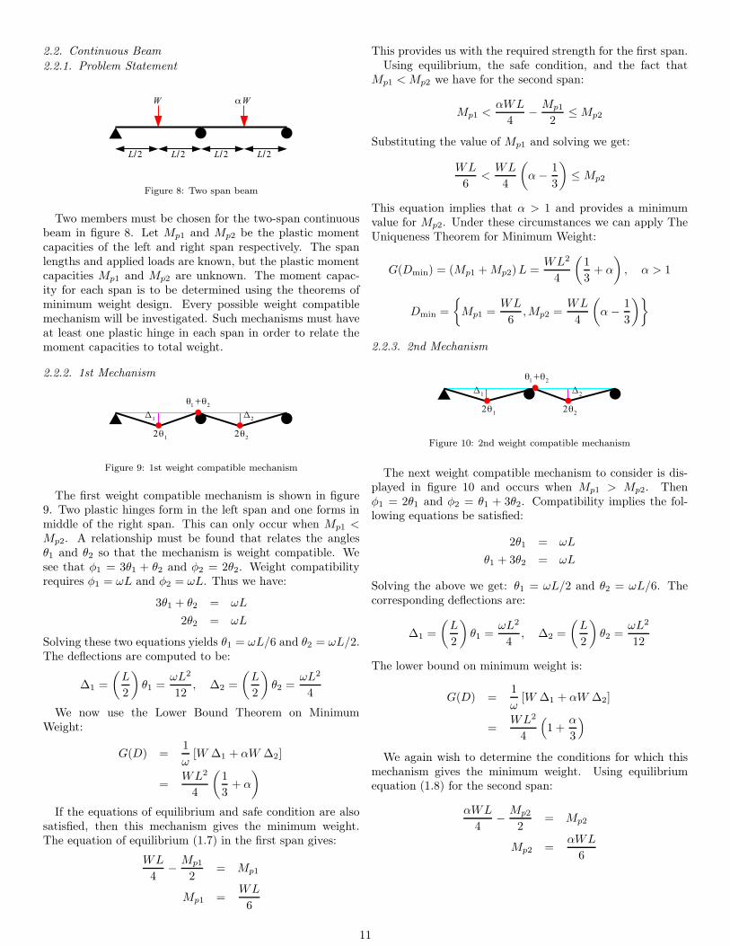
Two members must be chosen for the two-span continuousbeam in figure 8. Let Mp1 and Mp2 be the plastic momentcapacities of the left and right span respectively. The spanlengths and applied loads are known, but the plastic momentcapacities Mp1 and Mp2 are unknown. The moment capac-ity for each span is to be determined using the theorems ofminimum weight design. Every possible weight compatiblemechanism will be investigated. Such mechanisms must haveat least one plastic hinge in each span in order to relate themoment capacities to total weight.

2.2.2. 1st Mechanism

Figure 9: 1st weight compatible mechanism

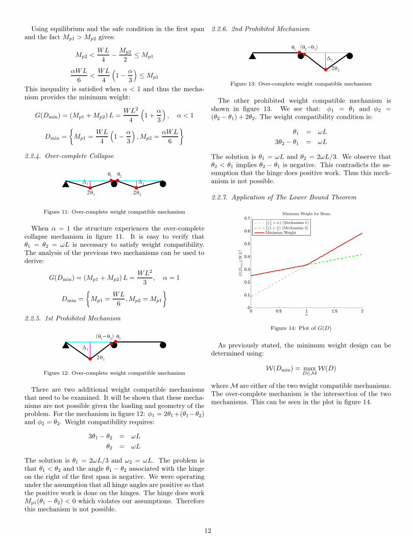
The first weight compatible mechanism is shown in figure9. Two plastic hinges form in the left span and one forms inmiddle of the right span. This can only occur when Mp1 <Mp2. A relationship must be found that relates the anglesθ1 and θ2 so that the mechanism is weight compatible. Wesee that φ1 = 3θ1 + θ2 and φ2 = 2θ2. Weight compatibilityrequires φ1 = ωL and φ2 = ωL. Thus we have:

3θ1 + θ2 = ωL

2θ2 = ωL

Solving these two equations yields θ1 = ωL/6 and θ2 = ωL/2.The deflections are computed to be:

∆1 =

(

L

2

)

θ1 =ωL2

12, ∆2 =

(

L

2

)

θ2 =ωL2

4

We now use the Lower Bound Theorem on MinimumWeight:

G(D) =1

ω[W ∆1 + αW ∆2]

=WL2

4

(

1

3+ α

)

If the equations of equilibrium and safe condition are alsosatisfied, then this mechanism gives the minimum weight.The equation of equilibrium (1.7) in the first span gives:

WL

4−

Mp1

2= Mp1

Mp1 =WL

6

This provides us with the required strength for the first span.Using equilibrium, the safe condition, and the fact that

Mp1 < Mp2 we have for the second span:

Mp1 <αWL

4−

Mp1

2≤ Mp2

Substituting the value of Mp1 and solving we get:

WL

6<

WL

4

(

α−1

3

)

≤ Mp2

This equation implies that α > 1 and provides a minimumvalue for Mp2. Under these circumstances we can apply TheUniqueness Theorem for Minimum Weight:

G(Dmin) = (Mp1 +Mp2)L =WL2

4

(

1

3+ α

)

, α > 1

Dmin =

{

Mp1 =WL

6,Mp2 =

WL

4

(

α−1

3

)}

2.2.3. 2nd Mechanism

Figure 10: 2nd weight compatible mechanism

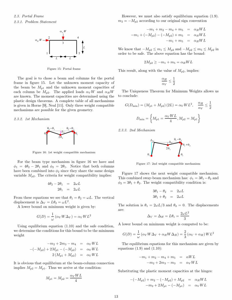
The next weight compatible mechanism to consider is dis-played in figure 10 and occurs when Mp1 > Mp2. Thenφ1 = 2θ1 and φ2 = θ1 + 3θ2. Compatibility implies the fol-lowing equations be satisfied:

2θ1 = ωL

θ1 + 3θ2 = ωL

Solving the above we get: θ1 = ωL/2 and θ2 = ωL/6. Thecorresponding deflections are:

∆1 =

(

L

2

)

θ1 =ωL2

4, ∆2 =

(

L

2

)

θ2 =ωL2

12

The lower bound on minimum weight is:

G(D) =1

ω[W ∆1 + αW ∆2]

=WL2

4

(

1 +α

3

)

We again wish to determine the conditions for which thismechanism gives the minimum weight. Using equilibriumequation (1.8) for the second span:

αWL

4−

Mp2

2= Mp2

Mp2 =αWL

6

11

Using equilibrium and the safe condition in the first spanand the fact Mp1 > Mp2 gives:

Mp2 <WL

4−

Mp2

2≤ Mp1

αWL

6<

WL

4

(

1−α

3

)

≤ Mp1

This inequality is satisfied when α < 1 and thus the mecha-nism provides the minimum weight:

G(Dmin) = (Mp1 +Mp2)L =WL2

4

(

1 +α

3

)

, α < 1

Dmin =

{

Mp1 =WL

4

(

1−α

3

)

,Mp2 =αWL

6

}

2.2.4. Over-complete Collapse

Figure 11: Over-complete weight compatible mechanism

When α = 1 the structure experiences the over-completecollapse mechanism in figure 11. It is easy to verify thatθ1 = θ2 = ωL is necessary to satisfy weight compatibility.The analysis of the previous two mechanisms can be used toderive:

G(Dmin) = (Mp1 +Mp2)L =WL2

3, α = 1

Dmin =

{

Mp1 =WL

6,Mp2 = Mp1

}

2.2.5. 1st Prohibited Mechanism

Figure 12: Over-complete weight compatible mechanism

There are two additional weight compatible mechanismsthat need to be examined. It will be shown that these mecha-nisms are not possible given the loading and geometry of theproblem. For the mechanism in figure 12: φ1 = 2θ1+(θ1−θ2)and φ2 = θ2. Weight compatibility requires:

3θ1 − θ2 = ωL

θ2 = ωL

The solution is θ1 = 2ωL/3 and ω2 = ωL. The problem isthat θ1 < θ2 and the angle θ1 − θ2 associated with the hingeon the right of the first span is negative. We were operatingunder the assumption that all hinge angles are positive so thatthe positive work is done on the hinges. The hinge does workMp1(θ1 − θ2) < 0 which violates our assumptions. Thereforethis mechanism is not possible.

2.2.6. 2nd Prohibited Mechanism

Figure 13: Over-complete weight compatible mechanism

The other prohibited weight compatible mechanism isshown in figure 13. We see that: φ1 = θ1 and φ2 =(θ2 − θ1) + 2θ2. The weight compatibility condition is:

θ1 = ωL

3θ2 − θ1 = ωL

The solution is θ1 = ωL and θ2 = 2ωL/3. We observe thatθ2 < θ1 implies θ2 − θ1 is negative. This contradicts the as-sumption that the hinge does positive work. Thus this mech-anism is not possible.

2.2.7. Application of The Lower Bound Theorem

0 0.5 1 1.5 20

0.1

0.2

0.3

0.4

0.5

0.6

0.7

α

G(D

min)/W

L2

Minimum Weight for Beam

14(

13 + α) (Mechanism 1)

14(1 +

α

3 ) (Mechanism 2)Minimum Weight

Figure 14: Plot of G(D)

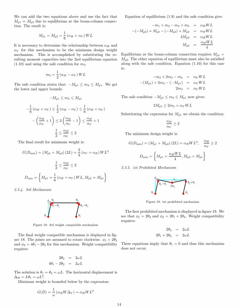
As previously stated, the minimum weight design can bedetermined using:

W(Dmin) = maxD∈M

W(D)

where M are either of the two weight compatible mechanisms.The over-complete mechanism is the intersection of the twomechanisms. This can be seen in the plot in figure 14.

12

2.3. Portal Frame

2.3.1. Problem Statement

Figure 15: Portal frame

The goal is to chose a beam and columns for the portalframe in figure 15. Let the unknown moment capacity ofthe beam be Mp1 and the unknown moment capacities ofeach column be Mp2. The applied loads αV W and αHWare known. The moment capacities are determined using theplastic design theorems. A complete table of all mechanismsis given in Horne [9], Neal [11]. Only three weight compatiblemechanisms are possible for the given geometry.

2.3.2. 1st Mechanism

Figure 16: 1st weight compatible mechanism

For the beam type mechanism in figure 16 we have andφ1 = 4θ2 − 2θ1 and φ2 = 2θ1. Notice that both columnshave been combined into φ2 since they share the same designvariable Mp2. The criteria for weight compatibility implies:

4θ2 − 2θ1 = 2ωL

2θ1 = 2ωL

From these equations we see that θ1 = θ2 = ωL. The verticaldisplacement is ∆V = Lθ2 = ωL2.

A lower bound on minimum weight is given by:

G(D) =1

ω(αV W∆V ) = αV WL2

Using equilibrium equation (1.10) and the safe condition,we determine the conditions for this bound to be the minimumweight

−m2 + 2m3 −m4 = αV WL

−(−Mp2) + 2Mp1 − (−Mp2) = αV WL

2 (Mp1 +Mp2) = αV WL

It is obvious that equilibrium at the beam-column connectionimplies Mp2 = Mp1. Thus we arrive at the condition:

Mp1 = Mp2 =αV WL

4

However, we must also satisfy equilibrium equation (1.9).m2 = −Mp2 according to our original sign convention

−m1 +m2 −m4 +m5 = αHWL

−m1 + (−Mp2)− (−Mp2) +m5 = αHWL

−m1 +m5 = αHWL

We know that −Mp2 ≤ m1 ≤ Mp2 and −Mp2 ≤ m5 ≤ Mp2 inorder to be safe. The above equation has the bound:

2Mp2 ≥ −m1 +m5 = αHWL

This result, along with the value of Mp2, implies:

αH

αV

≤1

2

The Uniqueness Theorem for Minimum Weights allows usto conclude:

G(Dmin) = (Mp1 +Mp2) (2L) = αV WL2,αH

αV

≤1

2

Dmin =

{

Mp1 =αV WL

4,Mp2 = Mp1

}

2.3.3. 2nd Mechanism

Figure 17: 2nd weight compatible mechanism

Figure 17 shows the next weight compatible mechanism.This combined sway-beam mechanism has: φ1 = 3θ1−θ2 andφ2 = 3θ1 + θ2. The weight compatibility condition is:

3θ1 − θ2 = 2ωL

3θ1 + θ2 = 2ωL

The solution is θ1 = 2ωL/3 and θ2 = 0. The displacementsare:

∆V = ∆H = Lθ1 =2ωL2

3

A lower bound on minimum weight is computed to be:

G(D) =1

ω(αV W∆V + αHW∆H) =

2

3(αV + αH)WL2

The equilibrium equations for this mechanism are given byequations (1.9) and (1.10):

−m1 +m2 −m4 +m5 = αWL

−m2 + 2m3 −m3 = αV WL

Substituting the plastic moment capacities at the hinges:

−(−Mp2) +m2 − (−Mp2) +Mp2 = αHWL

−m2 + 2Mp1 − (−Mp1) = αV WL

13

We can add the two equations above and use the fact thatMp1 = Mp2 due to equilibrium at the beam-column connec-tion. The result is:

Mp1 = Mp2 =1

6(αH + αV )WL

It is necessary to determine the relationship between αH andαV for this mechanism to be the minimum design weightmechanism. This is accomplished by substituting the re-sulting moment capacities into the 2nd equilibrium equation(1.10) and using the safe condition for m2.

m2 =1

2(αH − αV )WL

The safe condition states that: −Mp1 ≤ m2 ≤ Mp1. We getthe lower and upper bounds:

−Mp1 ≤ m2 ≤ Mp1

−1

6(αH + αV ) ≤

1

2(αH − αV ) ≤

1

6(αH + αV )

−

(

αH

αV

+ 1

)

≤ 3

(

αH

αV

− 1

)

≤αH

αV

+ 1

1

2≤

αH

αV

≤ 2

The final result for minimum weight is:

G(Dmin) = (Mp1 +Mp2) (2L) =2

3(αV + αH)WL2

1

2≤

αH

αV

≤ 2

Dmin =

{

Mp1 =1

6(αH + αV )WL,Mp2 = Mp1

}

2.3.4. 3rd Mechanism

Figure 18: 3rd weight compatible mechanism

The final weight compatible mechanism is displayed in fig-ure 18. The joints are assumed to rotate clockwise. φ1 = 2θ2and φ2 = 4θ1− 2θ2 for this mechanism. Weight compatibilityrequires:

2θ2 = 2ωL

4θ1 − 2θ2 = 2ωL

The solution is θ1 = θ2 = ωL. The horizontal displacement is∆H = Lθ1 = ωL2.

Minimum weight is bounded below by the expression:

G(D) =1

ω(αHW∆V ) = αHWL2

Equation of equilibrium (1.9) and the safe condition give:

−m1 +m2 −m4 +m5 = αHWL

−(−Mp2) +Mp2 − (−Mp2) +Mp2 = αHWL

4Mp2 = αHWL

Mp2 =αHWL

4

Equilibrium at the beam-column connection requires Mp1 =Mp2. The other equation of equilibrium must also be satisfiedalong with the safe condition. Equation (1.10) for this caseis:

−m2 + 2m3 −m4 = αV WL

−(Mp1) + 2m3 − (−Mp1) = αV WL

2m3 = αV WL

The safe condition −Mp1 ≤ m3 ≤ Mp1 now gives:

2Mp1 ≥ 2m3 = αV WL

Substituting the expression for Mp1 we obtain the condition:

αH

αV

≥ 2

The minimum design weight is:

G(Dmin) = (Mp1 +Mp2) (2L) = αHWL2,αH

αV

≥ 2

Dmin =

{

Mp1 =αHWL

4,Mp2 = Mp1

}

2.3.5. 1st Prohibited Mechanism

Figure 19: 1st prohibited mechanism

The first prohibited mechanism is displayed in figure 19. Wesee that φ1 = 2θ2 and φ2 = 2θ1 + 2θ2. Weight compatibilityrequires:

2θ2 = 2ωL

2θ1 + 2θ2 = 2ωL

These equations imply that θ1 = 0 and thus this mechanismdoes not occur.

14

2.3.6. 2nd Prohibited Mechanism

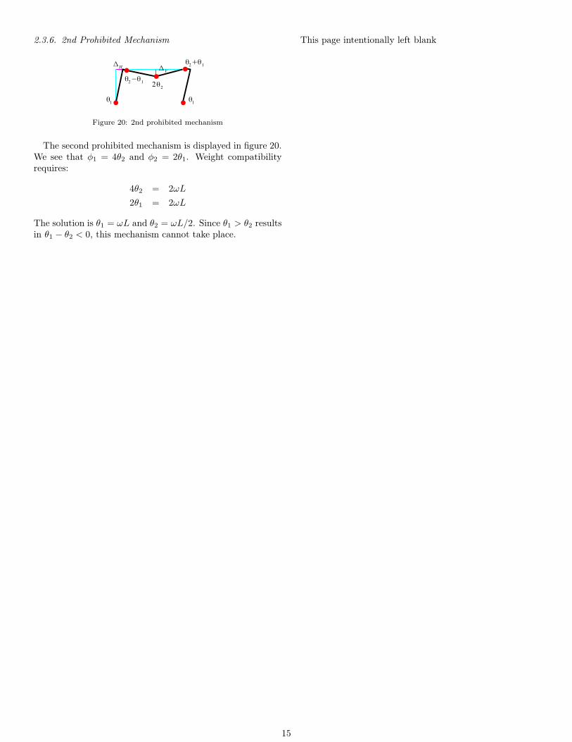
Figure 20: 2nd prohibited mechanism

The second prohibited mechanism is displayed in figure 20.We see that φ1 = 4θ2 and φ2 = 2θ1. Weight compatibilityrequires:

4θ2 = 2ωL

2θ1 = 2ωL

The solution is θ1 = ωL and θ2 = ωL/2. Since θ1 > θ2 resultsin θ1 − θ2 < 0, this mechanism cannot take place.

This page intentionally left blank

15

3. Variable Repeated Loading

3.1. Formulation

3.1.1. Introduction

All of the previous statements concerning plastic analysisand design had assumed that the applied loads were static.This includes the case where the loads are gradually increasedfrom zero. The increase in loading is gradual enough thatdynamic effects can be ignored. Thus we were dealing withproblems of statics. However, many loading situations aredynamic. Examples of dynamic loads are wind and seismicloads. Fortunately, a complete time-dependent solution isusually not required in order to determine the conditions ofcollapse. We only require knowledge of the magnitude of theapplied loads and their possible combinations. Details of theorder or duration of loading is not needed. Under such condi-tions, collapse can occur at lower values of load than for thestatic cases previously explored. The goal is to state theo-rems that inform us to the nature of the collapse. We firstdefine two types of collapse and then provide motivation witha detailed example.

The simplest case to consider is one where loads are applied,removed, and then applied in the opposite direction. If thiscycle is repeated, it is possible for a frame to collapse dueto fracture of certain members. The members are bent backand forth. The alternating between yielding in tension andyielding in compression eventually results in fracture. Thisdefines a particular condition of collapse defined below.

Definition 3.1. If any members of a frame fail due to alter-nating application of applied loads, then the frame has faileddue to alternating plasticity.

Alternating plasticity usually only occurs for structures incyclical loading that are subject to fatigue. A more commonsituation is one in which loads are variable but not alternating.

Definition 3.2. Suppose that a frame is subjected to variablerepeated loads. If plastic hinge rotations continue to increasewithout bound, then the frame will fail due to incrementalcollapse.

The fact that plastic hinge rotations increase during incre-mental collapse suggests behavior similar to a collapse mech-anism. Unlike an ordinary collapse mechanism, all of thehinges are not present simultaneously in an incremental col-lapse mechanism. Instead, the deformations increase in amanner that mimics a collapse mechanism. This is explainedin further detail in the next section.

If a frame does not fail due to alternating plasticity orincremental collapse, then the plastic hinge rotations re-main bounded. Thus no incremental collapse mechanisms areformed. This situation renders the structure safe.

Definition 3.3. Suppose during application of variable re-peated loads, a frame ceases to produce additional plastichinge rotation and all subsequent changes of bending mo-ments are entirely elastic. Then the frame is said to haveshaken down.

It should be noted that shakedown might be approachedinstead of reached. This occurs when the increments of plastichinge rotation decrease in magnitude over time in a mannersuch that the total hinge rotation is bounded.

This page intentionally left blank

16

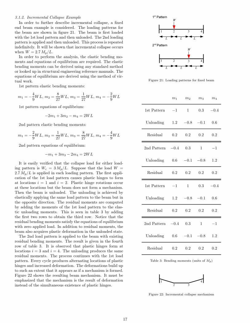
3.1.2. Incremental Collapse Example

In order to further describe incremental collapse, a fixedend beam example is considered. The loading patterns forthe beam are shown in figure 21. The beam is first loadedwith the 1st load pattern and then unloaded. The 2nd loadingpattern is applied and then unloaded. This process is repeatedindefinitely. It will be shown that incremental collapse occurswhen W = 2.7Mp/L.

In order to perform the analysis, the elastic bending mo-ments and equations of equilibrium are required. The elasticbending moments can be derived using any standard methodor looked up in structural engineering reference manuals. Theequations of equilibrium are derived using the method of vir-tual work.

1st pattern elastic bending moments:

m1 = −4

9WL, m2 =

8

27WL, m3 =

1

27WL, m4 = −

2

9WL

1st pattern equations of equilibrium:

−2m1 + 3m2 −m4 = 2WL

2nd pattern elastic bending moments:

m1 = −2

9WL, m2 =

1

27WL, m3 =

8

27WL, m4 = −

4

9WL

2nd pattern equations of equilibrium:

−m1 + 3m3 − 2m4 = 2WL

It is easily verified that the collapse load for either load-ing pattern is Wc = 3Mp/L. Suppose that the load W =2.7Mp/L is applied in each loading pattern. The first appli-cation of the 1st load pattern causes plastic hinges to format locations i = 1 and i = 2. Plastic hinge rotations occurat these locations but the beam does not form a mechanism.Then the beam is unloaded. The unloading is achieved byelastically applying the same load pattern to the beam but inthe opposite direction. The residual moments are computedby adding the moments of the 1st load pattern to the elas-tic unloading moments. This is seen in table 3 by addingthe first two rows to obtain the third row. Notice that theresidual bending moments satisfy the equations of equilibriumwith zero applied load. In addition to residual moments, thebeam also acquires plastic deformation in the unloaded state.

The 2nd load pattern is applied to the beam with existingresidual bending moments. The result is given in the fourthrow of table 3. It is observed that plastic hinges form atlocations i = 3 and i = 4. The unloading produces the sameresidual moments. The process continues with the 1st loadpattern. Every cycle produces alternating locations of plastichinges and increased deformation. The deformations build upto such an extent that it appears as if a mechanism is formed.Figure 22 shows the resulting beam mechanism. It must beemphasized that the mechanism is the result of deformationinstead of the simultaneous existence of plastic hinges.

Figure 21: Loading patterns for fixed beam

m1 m2 m3 m4

1st Pattern −1 1 0.3 −0.4

Unloading 1.2 −0.8 −0.1 0.6

Residual 0.2 0.2 0.2 0.2

2nd Pattern −0.4 0.3 1 −1

Unloading 0.6 −0.1 −0.8 1.2

Residual 0.2 0.2 0.2 0.2

1st Pattern −1 1 0.3 −0.4

Unloading 1.2 −0.8 −0.1 0.6

Residual 0.2 0.2 0.2 0.2

2nd Pattern −0.4 0.3 1 −1

Unloading 0.6 −0.1 −0.8 1.2

Residual 0.2 0.2 0.2 0.2

Table 3: Bending moments (units of Mp)

Figure 22: Incremental collapse mechanism

17

3.1.3. Theorems

In order to state the Shakedown Theorem, a few items ofnotation are introduced. Let Mmax

i and Mmin

i be the max-imum and minimum elastic bending moments that occur atlocation i for any combination of applied loads. These mo-ments are computed from an initial stress-free state and canbe positive or negative. The fact that they are elastic bend-ing moments means that their absolute value can exceed the

plastic moment capacity MK(i)p . The value at which plastic

yielding begins is notated as MK(i)y . For the ideal elastic-

plastic relationship, we set MK(i)y = M

K(i)p .

Let mi be the actual bending moments during a particularstage of the loading process. If Mi is the elastic bendingmoment under the same loads, then m̄i = mi − Mi are theresidual bending moments. The residual bending momentsm̄i are statically admissible if they satisfy equilibrium whenthere are no applied loads.

Theorem 3.1 (Shakedown Theorem). If it is possible to finda distribution of residual bending moments m̄∗

i that are stati-cally admissible and satisfy the following inequalities, then theframe will eventually shake down.

m̄∗i +Mmax

i ≤ MK(i)p (3.1)

m̄∗i +Mmin

i ≥ −MK(i)p (3.2)

Mmax

i −Mmin

i ≤ 2MK(i)y (3.3)

Proof. Let m̄(x) = m(x)−M(x) be the actual residual bend-ing moments during a particular instant in the loading pro-cess. Assume that m̄∗

i are the postulated residual bendingmoments of the theorem. Define the quantity U as follows:

U =

Nmembers∑

k=1

ˆ Lk

0

(m̄− m̄∗)2

2EIdx (3.4)

It is obvious that U ≥ 0.Suppose a small change in loading occurs. Then the change

in residual moments is δm̄ = δm − δM. The correspondingchange in U is:

δU =

Nmembers∑

k=1

ˆ Lk

0

(m̄− m̄∗)δm̄

EIdx (3.5)

Any change in the residual moments is due to plastic hingerotations. Let Np be the number of plastic hinges and δθjbe the increments of plastic hinge rotation. If the residualmoments m̄ and m̄∗ are in equilibrium with zero externalloads, then the same is true for m̄ − m̄∗. Thus we have thecomplementary work equation:

Nmembers∑

k=1

ˆ Lk

0

(m̄− m̄∗)δm̄

EIdx +

Np∑

j=1

(m̄j − m̄∗j )δθj = 0 (3.6)

Notice that the first term in equation (3.6) is due to elasticchanges within members and the second term is due to plastichinge rotations. Comparing equations (3.5) and (3.6) we get:

δU = −

Np∑

j=1

(m̄j − m̄∗j )δθj (3.7)

Suppose m̄j < m̄∗j at a particular hinge location j. Then

by equation (3.1), we have:

m̄j +Mmax

j < MK(j)p

Since m̄j +Mmax

j is the largest possible value of bending mo-ment at location j, the plastic hinge cannot have the pos-

itive value MK(j)p . Thus the hinge formed at a value of

−MK(j)p and the corresponding hinge rotation δθj must be

negative. The corresponding term in equation (3.7) is posi-tive: (m̄j − m̄∗

j )δθj > 0.If m̄j > m̄∗

j at hinge location j. Then by equation (3.2),we have:

m̄j +Mmin

j > −MK(j)p

Now m̄j + Mmin

j is the smallest possible value of bendingmoment at location j. The plastic hinge cannot have the

negative value −MK(j)p . Thus the hinge formed at a value

of MK(j)p and the corresponding hinge rotation δθj must be

positive. The corresponding term in equation (3.7) is againpositive: (m̄j − m̄∗

j )δθj > 0.Lastly, m̄j = m̄∗

j implies (m̄j − m̄∗j )δθj = 0.

Thus every term in the sum appearing in equation (3.7) isnon-negative and we have:

δU ≤ 0 (3.8)

When the behavior of the frame is entirely elastic, thenδθj = 0 and thus δU = 0. U can decrease only during plas-tic deformation. Combining these results with the fact thatU ≥ 0 shows that U approaches a non-negative constant. Thisimplies that the frame approaches shakedown. If it happensthat U approaches 0, then the postulated residual bendingmoments m̄∗

i are the actual residual bending moments m̄i atshakedown. The inequality (3.3) ensures that the frame doesnot fail due to alternating plasticity.

Several points concerning this theorem are provided byHorne [9] and are worth repeating here:

• The postulated moments m̄∗i are not necessarily the ac-

tual residual moments after shakedown. The proof of thetheorem did not require knowledge of the final residualmoments.

• The initial state of stress does not affect the condition ofshakedown. However, the number of load variations toreach shakedown may change due to the initial stresses.

• The order in which the loads are applied does not affectthe condition of shakedown. The order of applied loadsmay change how quickly a frame shakes down.

• The theorem does not state how many load variationsare required for shakedown to occur. It is possible thatshakedown is approached but never reached in a finitenumber of load variations.

• Thermal strains can be incorporated into the formulationof the Shakedown Theorem. The corresponding thermalstresses are added to Mmax

i and Mmin

i .

18

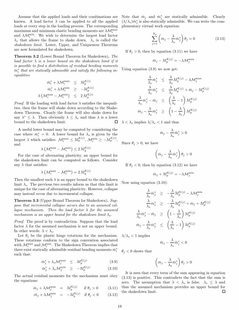
Assume that the applied loads and their combinations areknown. A load factor λ can be applied to all the appliedloads at every step in the loading process. The correspondingmaximum and minimum elastic bending moments are λMmax

i

and λMmin

i . We wish to determine the largest load factorλs that allows the frame to shake down. λs is called theshakedown limit. Lower, Upper, and Uniqueness Theoremsare now formulated for shakedown.

Theorem 3.2 (Lower Bound Theorem for Shakedown). Theload factor λ is a lower bound on the shakedown limit if itis possible to find a distribution of residual bending momentsm̄∗

i that are statically admissible and satisfy the following in-equalities

m̄∗i + λMmax

i ≤ MK(i)p

m̄∗i + λMmin

i ≥ −MK(i)p

λ(

Mmax

i −Mmin

i

)

≤ 2MK(i)y

Proof. If the loading with load factor λ satisfies the inequali-ties, then the frame will shake down according to the Shake-down Theorem. Clearly the frame will also shake down forany λ∗ ≤ λ. Then obviously λ ≤ λs and thus λ is a lowerbound to the shakedown limit.

A useful lower bound may be computed by considering thecase where m̄∗

i = 0. A lower bound for λs is given by the

largest λ which satisfies: Mmaxi ≤ M

K(i)p , Mmin

i ≥ −MK(i)p ,

andλ(

Mmax

i −Mmin

i

)

≤ 2MK(i)y

For the case of alternating plasticity, an upper bound forthe shakedown limit can be computed as follows. Considerany λ that satisfies:

λ(

Mmax

i −Mmin

i

)

= 2MK(i)y

Then the smallest such λ is an upper bound to the shakedownlimit λs. The previous two results inform us that this limit isunique for the case of alternating plasticity. However, collapsemay instead occur due to incremental collapse.

Theorem 3.3 (Upper Bound Theorem for Shakedown). Sup-pose that incremental collapse occurs due to an assumed col-lapse mechanism. Then the load factor λ for the assumedmechanism is an upper bound for the shakedown limit λs.

Proof. The proof is by contradiction. Suppose that the loadfactor λ for the assumed mechanism is not an upper bound.In other words: λ < λs.

Let θj be the plastic hinge rotations for the mechanism.These rotations conform to the sign convention associatedwith Mmax

i and Mmin

i . The Shakedown Theorem implies thatthere exist statically admissible residual bending moments m̄∗

i

such that:

m̄∗j + λsM

max

j ≤ MK(j)p (3.9)

m̄∗j + λsM

min

j ≥ −MK(j)p (3.10)

The actual residual moments for the mechanism must obeythe equations:

m̄j + λMmax

j = MK(j)p if θj > 0 (3.11)

m̄j + λMmin

j = −MK(j)p if θj < 0 (3.12)

Note that m̄j and m̄∗j are statically admissible. Clearly

(λ/λs)m̄∗j is also statically admissible. We can write the com-

plementary virtual work equation:

Np∑

j=1

(

m̄j −λ

λs

m̄∗j

)

θj = 0 (3.13)

If θj > 0, then by equation (3.11) we have

m̄j −MK(j)p = −λMmax

j

Using equation (3.9) we now get:

λ

λs

m̄∗j ≤

λ

λs

MK(j)p − λMmax

j

λ

λs

m̄∗j ≤

λ

λs

MK(j)p + m̄j −MK(j)

p

λ

λs

m̄∗j − m̄j ≤

(

λ

λs

− 1

)

MK(j)p

m̄j −λ

λs

m̄∗j ≥

(

1−λ

λs

)

MK(j)p

λ < λs implies λ/λs < 1 and thus

m̄j −λ

λs

m̄∗j > 0

Since θj > 0, we have

(

m̄j −λ

λs

m̄∗j

)

θj > 0

If θj < 0, then by equation (3.12) we have

m̄j +MK(j)p = −λMmin

j

Now using equation (3.10):

λ

λs

m̄∗j ≥ −

λ

λs

MK(j)p − λMmin

j

λ

λs

m̄∗j ≥ −

λ

λs

MK(j)p + m̄j +MK(j)

p

λ

λs

m̄∗j − m̄j ≥

(

1−λ

λs

)

MK(j)p

m̄j −λ

λs

m̄∗j ≤

(

λ

λs

− 1

)

MK(j)p

λ/λs < 1 implies

m̄j −λ

λs

m̄∗j < 0

θj < 0 shows that

(

m̄j −λ

λs

m̄∗j

)

θj > 0

It is seen that every term of the sum appearing in equation(3.13) is positive. This contradicts the fact that the sum iszero. The assumption that λ < λs is false. λs ≤ λ andthus the assumed mechanism provides an upper bound forthe shakedown limit.

19

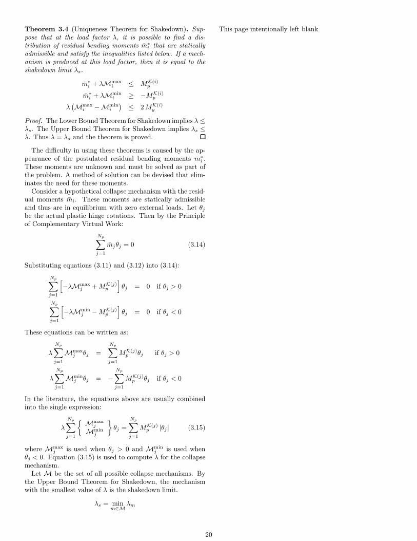
Theorem 3.4 (Uniqueness Theorem for Shakedown). Sup-pose that at the load factor λ, it is possible to find a dis-tribution of residual bending moments m̄∗

i that are staticallyadmissible and satisfy the inequalities listed below. If a mech-anism is produced at this load factor, then it is equal to theshakedown limit λs.

m̄∗i + λMmax

i ≤ MK(i)p

m̄∗i + λMmin

i ≥ −MK(i)p

λ(

Mmax

i −Mmin

i

)

≤ 2MK(i)y

Proof. The Lower Bound Theorem for Shakedown implies λ ≤λs. The Upper Bound Theorem for Shakedown implies λs ≤λ. Thus λ = λs and the theorem is proved.

The difficulty in using these theorems is caused by the ap-pearance of the postulated residual bending moments m̄∗

i .These moments are unknown and must be solved as part ofthe problem. A method of solution can be devised that elim-inates the need for these moments.

Consider a hypothetical collapse mechanism with the resid-ual moments m̄i. These moments are statically admissibleand thus are in equilibrium with zero external loads. Let θjbe the actual plastic hinge rotations. Then by the Principleof Complementary Virtual Work:

Np∑

j=1

m̄jθj = 0 (3.14)

Substituting equations (3.11) and (3.12) into (3.14):

Np∑

j=1

[

−λMmax

j +MK(j)p

]

θj = 0 if θj > 0

Np∑

j=1

[

−λMmin

j −MK(j)p

]

θj = 0 if θj < 0

These equations can be written as:

λ

Np∑

j=1

Mmax

j θj =

Np∑

j=1

MK(j)p θj if θj > 0

λ

Np∑

j=1

Mmin

j θj = −

Np∑

j=1

MK(j)p θj if θj < 0

In the literature, the equations above are usually combinedinto the single expression:

λ

Np∑

j=1

{

Mmax

j

Mmin

j

}

θj =

Np∑

j=1

MK(j)p |θj | (3.15)

where Mmax

j is used when θj > 0 and Mmin

j is used whenθj < 0. Equation (3.15) is used to compute λ for the collapsemechanism.

Let M be the set of all possible collapse mechanisms. Bythe Upper Bound Theorem for Shakedown, the mechanismwith the smallest value of λ is the shakedown limit.

λs = minm∈M

λm

This page intentionally left blank

20

3.2. Continuous Beam

The continuous beam shown in figure 23 is subjected to arepeated loading pattern. The 1st loading pattern is followedby complete unloading. Then the 2nd loading pattern is ap-plied and unloaded. This cycle is repeated indefinitely. Wewish to determine the maximum load factor λs for shakedownto occur. Every possible beam mechanism is explored usingequation (3.15).

3.2.1. 1st Beam Mechanism

We first consider a beam mechanism in the left span. Ap-plying equation (3.15) to this mechanism results in the fol-lowing expression:

λ[

Mmax

1 (2θ) +Mmin

2 (−θ)]

= 3Mpθ

λ

[(

5

32WL

)

(2θ) +

(

−3

16WL

)

(−θ)

]

= 3Mpθ

Solving for λ we get:

λ = 6Mp

WL

3.2.2. 2nd Beam Mechanism

For a beam mechanism in the right span we have:

λ[

Mmin

2 (−θ) +Mmax

3 (2θ)]

= 3Mpθ

λ

[(

−3

16WL

)

(−θ) +

(

13

64WL

)

(2θ)

]

= 3Mpθ

The solution is for λ is:

λ =96

19

Mp

WL≈ 5.05

Mp

WL

3.2.3. Over-complete Collapse

Lastly, we investigate the case of beam mechanisms in bothspans.

λ[

Mmax

1 (2θ) +Mmin

2 (−2θ) +Mmax

3 (2θ)]

= 6Mpθ

λ

[(

5

32WL

)

(2θ) +

(

−3

16WL

)

(−2θ) +

(

13

64WL

)

(2θ)

]

= 6Mpθ

Again solving for λ we have:

λ =192

35

Mp

WL≈ 5.49

Mp

WL

The smallest λ for all the mechanisms is the shakedownlimit and the corresponding mechanism is the actual collapsemechanism. Thus we observe that collapse occurs for a beammechanism in the right span and the shakedown limit is:

λs =96

19

Mp

WL

3.2.4. Alternating Plasticity

It is also necessary to ensure that the beam does not fail dueto alternating plasticity. The third condition for shakedownis applied at every possible plastic hinge location.

For i = 1:

λ(

Mmax −Mmin)

= 2Mp

λ

(

13

64WL

)

= 2Mp

λ =128

13

Mp

WL≈ 9.85

Mp

WL

Figure 23: Loading patterns for beam

i = 1 i = 2 i = 3

1st Pattern 532 − 3

16532

2nd Pattern − 364 − 3

321364

Zero Loading 0 0 0

Mmax 532 0 13

64

Mmin − 364 − 3

16532

Mmax −Mmin 1364

316

364

Table 4: Elastic bending moments (units of WL)

For i = 2:

λ(

Mmax −Mmin)

= 2Mp

λ

(

3

16WL

)

= 2Mp

λ =32

3

Mp

WL≈ 10.67

Mp

WL

For i = 3:

λ(

Mmax −Mmin)

= 2Mp

λ

(

3

64WL

)

= 2Mp

λ =128

3

Mp

WL≈ 42.67

Mp

WL

Since each λ for alternating collapse is larger than the shake-down limit λs, the beam fails by incremental collapse and notby alternating plasticity.

21

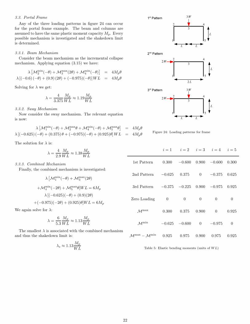
3.3. Portal Frame

Any of the three loading patterns in figure 24 can occurfor the portal frame example. The beam and columns areassumed to have the same plastic moment capacity Mp. Everypossible mechanism is investigated and the shakedown limitis determined.

3.3.1. Beam Mechanism

Consider the beam mechanism as the incremental collapsemechanism. Applying equation (3.15) we have:

λ[

Mmin

2 (−θ) +Mmax

3 (2θ) +Mmin

4 (−θ)]

= 4Mpθ

λ [(−0.6) (−θ) + (0.9) (2θ) + (−0.975)(−θ)]WL = 4Mpθ

Solving for λ we get:

λ =4

3.375

Mp

WL≈ 1.19

Mp

WL

3.3.2. Sway Mechanism

Now consider the sway mechanism. The relevant equationis now:

λ[

Mmin

1 (−θ) +Mmax

2 θ +Mmin

4 (−θ) +Mmax

5 θ]

= 4Mpθ

λ [(−0.625) (−θ) + (0.375) θ + (−0.975)(−θ) + (0.925)θ]WL = 4Mpθ

The solution for λ is:

λ =4

2.9

Mp

WL≈ 1.38

Mp

WL

3.3.3. Combined Mechanism

Finally, the combined mechanism is investigated:

λ[

Mmin

1 (−θ) +Mmax

3 (2θ)

+Mmin

4 (−2θ) +Mmax

5 θ]WL = 6Mp

λ [(−0.625)(−θ) + (0.9)(2θ)

+(−0.975)(−2θ) + (0.925)θ]WL = 6Mp

We again solve for λ:

λ =6

5.3

Mp

WL≈ 1.13

Mp

WL

The smallest λ is associated with the combined mechanismand thus the shakedown limit is:

λs ≈ 1.13Mp

WL

Figure 24: Loading patterns for frame

i = 1 i = 2 i = 3 i = 4 i = 5

1st Pattern 0.300 −0.600 0.900 −0.600 0.300

2nd Pattern −0.625 0.375 0 −0.375 0.625

3rd Pattern −0.375 −0.225 0.900 −0.975 0.925

Zero Loading 0 0 0 0 0

Mmax 0.300 0.375 0.900 0 0.925

Mmin −0.625 −0.600 0 −0.975 0

Mmax −Mmin 0.925 0.975 0.900 0.975 0.925

Table 5: Elastic bending moments (units of WL)

22

3.3.4. Alternating Plasticity

We also check the possibility of alternating plasticity.For i = 1 or i = 5:

λ(

Mmax −Mmin)

= 2Mp

λ (0.925WL) = 2Mp

λ =2

0.925

Mp

WL≈ 2.16

Mp

WL

For i = 2 or i = 4:

λ(

Mmax −Mmin)

= 2Mp

λ (0.975WL) = 2Mp

λ =2

0.975

Mp

WL≈ 2.05

Mp

WL

For i = 3:

λ(

Mmax −Mmin)

= 2Mp

λ (0.9WL) = 2Mp

λ =2

0.9

Mp

WL≈ 2.22

Mp

WL

All of the values for λ are larger than λs. Thus alternatingplasticity does not occur.

References

[1] John Baker and Jacques Heyman. Plastic Design ofFrames 1, Fundamentals. Cambridge University Press,Cambridge, England, 1969.

[2] Lynn S. Beedle. Plastic Design of Steel Frames. Wiley,London, 1958.

[3] Wai-Fah Chen and Toshio Atsuta. Theory of Beam-Columns, volume 1. McGraw-Hill, New York, 1976.

[4] Wai-Fah Chen and Toshio Atsuta. Theory of Beam-Columns, volume 2. McGraw-Hill, New York, 1976.

[5] Wai-Fah Chen and E.M. Lui. Structural Stability, Theoryand Implementation. Prentice-Hall, Upper Saddle River,New Jersey, 1987.

[6] Wai-Fah Chen and E.M. Lui. Stability Design of SteelFrames. CRC Press, Boca Raton, Florida, 1991.

[7] Jacques Heyman. Plastic Design of Frames 2, Applica-tions. Cambridge University Press, Cambridge, England,1971.

[8] Philip G. Hodge. Plastic Analysis of Structures.McGraw-Hill, New York, 1959.

[9] Michael R. Horne. Plastic Theory of Structures. M.I.T.Press, Cambridge, Massachusetts, 1971.

[10] W. McGuire. Steel Structures. Prentice-Hall, EnglewoodCliffs, New Jersey, 1968.

[11] B.G. Neal. The Plastic Methods of Structural Analysis.Wiley, New York, second edition, 1963.

23