1

PROJEKTKURS I ADAPTIV SIGNALBEHANDLING

Room Acoustics with associated fundamentals of acoustics

PURPOSE......................................................................................................................................2

1. INTRODUCTION.....................................................................................................................2

2. FUNDAMENTALS OF ACOUSTICS......................................................................................4

2.1. VIBRATIONS AND SOUND (WAVES) ..........................................................................................4 2.2 WAVE EQUATION ....................................................................................................................6

A. The equation of continuity.................................................................................................................6

B. The equation of motion (Euler’s equation).........................................................................................6

C. The equation of state.........................................................................................................................6

D. Equations of linear acoustics............................................................................................................7

E. Wave equation of linear acoustics.....................................................................................................7

F. Velocity potential ..............................................................................................................................8

2.3 SIMPLE SOLUTIONS OF THE WAVE EQUATION ............................................................................8 A. Plane traveling waves.......................................................................................................................9

B. Acoustic impedance and characteristic acoustic impedance...............................................................9

C. Spherical waves..............................................................................................................................10

D. Energy density, acoustic intensity, and acoustic power....................................................................11

E. Sound levels and decibel scales.......................................................................................................12

2.4 REFLECTION AND REFRACTION AT BOUNDARIES.....................................................................13 2.5 STANDING WAVES.................................................................................................................15

A. Reflection of plane wave at a flat rigid boundary.............................................................................15

B. Standing waves in the rectangular cavity.........................................................................................16

2.6. RAY ACOUSTICS (GEOMETRIC ACOUSTICS) ................................................................................17

3. ROOM ACOUSTICS.............................................................................................................. 18

3.1. SOUND IN ROOMS .................................................................................................................18 A. Direct sound and reverberant sound................................................................................................18

B. Anechoic chambers, reverberant chambers and reverberant rooms.................................................18

C. Impulse response of a reverberant room..........................................................................................19

D. A simple model for the growth of sound in a room...........................................................................20

E. Reverberation time..........................................................................................................................21

F. Radius of reverberation...................................................................................................................24

3.2. STANDING WAVES AND NORMAL MODES IN ROOMS................................................................25 A. Normal modes and eigenfrequencies in a rectangular room.............................................................25

B. Frequency distribution of room resonaces, and high frequency approximation................................26

2

Purpose The purpose of the lessons is to introduce the fundamental knowledge and principles on acoustics and room acoustics that are needed in conducting the projects in course PROJEKTKURS I ADAPTIV SIGNALBEHANDLING. The knowledge and principles are a basic tool for us to understand how rooms affect sound wave propagation, to design experiments for correctly measuring the acoustic properties of rooms, loudspeakers and microphones, to interpret the signals recorded by microphones or other sound receivers in rooms, and so on.

Fig. 1.1. Acoustic measurement in a room

1. Introduction

Let us start with two practical examples that are closely related with this project course of adaptive signal processing. These examples show what the room acoustics is used for. Example 1: Measurement of impulse response of a room The measurement is made using the setup and the rectangular room in Fig. 1.1. Suppose that the loudspeaker and the microphone both have ideal frequency characteristics so that the loudspeaker can generate impulse outputs (sound) and the microphone can receive this impulse sound undistortedly. Placing the loudspeaker and microphone as a certain distance as shown in Fig. 1.1, the measured result (the output from the microphone) may look like that shown in Fig. 1.2. In the figure, we can see (1) that for a single impulse output from the loudspeaker so many impulses are recorded by the microphone; (2) that the impulses become faded with time; (3) that the successive impulses get closer in spacing as time increases, and then become diffuse after a certain period (e.g., 110 ms). If the loudspeaker creates another impulse at a later instant, say 100 ms later than the first generation, the microphone will record both the second impulse response and the first one that is 100 ms earlier. Obviously, the second impulse sound response is disturbed by the reverberant part of the first one. Can we do something to suppress this disturbance by means of adaptive signal processing?

3

Fig. 1.2. Impulse response of a room at a certain position.

Example 2: Measurement of the frequency response of a rectangular room Now we place the loudspeaker in one corner of the rectangular room, and the microphone in a diagonally opposite corner. By slowly increasing the frequency supplied to the loudspeaker from 20 to 100 Hz and simultaneously recording the output of the microphone, the recorded result is in solid curve (see Fig. 1.3). In the figure, the dashed line corresponds to the output of the loudspeaker measured in an anechoic (echo-free) chamber. This example shows that the frequency response of the room is uneven. To obtain a true output of the loudspeaker, people may use an inverse filter to compensate for unevenness in the frequency response. This is the so-called sound equalization.

Fig. 1.3. Frequency response of a rectangular

room at low frequencies.

The problems in these two examples are to be investigated in the lessons on room acoustics. Because of the time limit of four lecture hours for such a big subject, however, the room acoustics to be presented here will be confined to the scope very close to the above-mentioned purpose and some relevant fundamentals of acoustics required by room acoustics. It will happen very often that the results are directly given without detailed derivations.

4

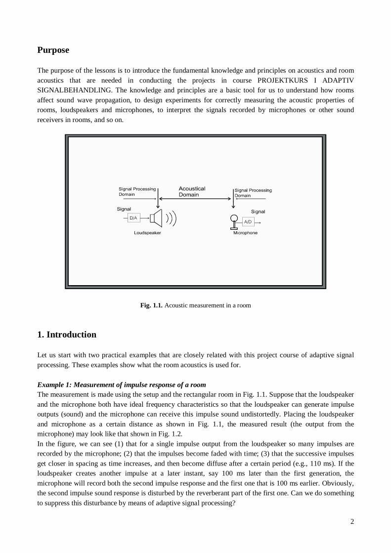
2. Fundamentals of acoustics

Fig. 2.1. A conversion process.

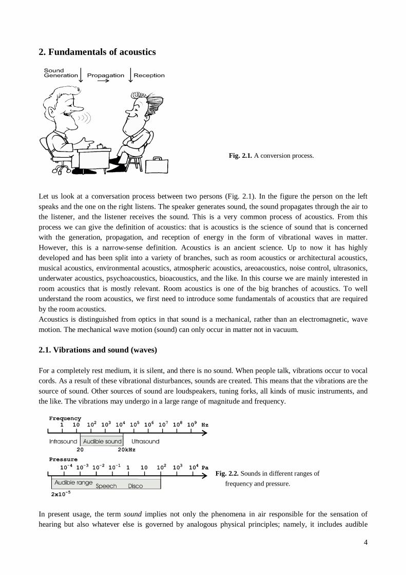
Let us look at a conversation process between two persons (Fig. 2.1). In the figure the person on the left speaks and the one on the right listens. The speaker generates sound, the sound propagates through the air to the listener, and the listener receives the sound. This is a very common process of acoustics. From this process we can give the definition of acoustics: that is acoustics is the science of sound that is concerned with the generation, propagation, and reception of energy in the form of vibrational waves in matter. However, this is a narrow-sense definition. Acoustics is an ancient science. Up to now it has highly developed and has been split into a variety of branches, such as room acoustics or architectural acoustics, musical acoustics, environmental acoustics, atmospheric acoustics, areoacoustics, noise control, ultrasonics, underwater acoustics, psychoacoustics, bioacoustics, and the like. In this course we are mainly interested in room acoustics that is mostly relevant. Room acoustics is one of the big branches of acoustics. To well understand the room acoustics, we first need to introduce some fundamentals of acoustics that are required by the room acoustics. Acoustics is distinguished from optics in that sound is a mechanical, rather than an electromagnetic, wave motion. The mechanical wave motion (sound) can only occur in matter not in vacuum. 2.1. Vibrations and sound (waves) For a completely rest medium, it is silent, and there is no sound. When people talk, vibrations occur to vocal cords. As a result of these vibrational disturbances, sounds are created. This means that the vibrations are the source of sound. Other sources of sound are loudspeakers, tuning forks, all kinds of music instruments, and the like. The vibrations may undergo in a large range of magnitude and frequency.

Fig. 2.2. Sounds in different ranges of

frequency and pressure.

In present usage, the term sound implies not only the phenomena in air responsible for the sensation of hearing but also whatever else is governed by analogous physical principles; namely, it includes audible

5

sound whose frequency lies in the range of about 20 to 20,000 Hz with pressure range of 510− ~100 Pa, infrasound with too low frequencies (<20 Hz) and ultrasound with too high frequencies (> 20 kHz) to be heard by a normal person (see Fig. 2.2). Sound travels in an elastic medium in a form of wave motion. Thus, it is also called sound wave. The medium can be gaseous, liquid, and solid. Waves can be of various types in terms of the directions of particle vibration and propagation. The term particle means a volume element large enough to contain millions of molecules so that the medium may be thought of as a continuous medium, yet small enough so that all physical variables may be considered nearly constant throughout the volume element. Of the most common types are longitudinal wave (also called compression wave) for which the directions of particle vibration and wave propagation are parallel, and transverse wave (or called shear wave) for which the directions are perpendicular (see Fig. 2.3). Sound waves propagating in air are longitudinal waves. Transverse waves can not propagate in air because air does not sustain transverse stress.

Longitudinal wave

Transverse wave

Fig. 2.3. Sound waves of two common types: longitudinal and transverse waves.

Sound wave is a physical phenomenon and process that is related with variations of pressure, particle velocity, density, and temperature. For example, for a medium in an equilibrium state in which there exists no sound, it has static pressure 0p (equilibrium pressure), and constant density 0ρ (equilibrium density). When a sound wave travels in the medium, the pressure and density in the medium are changed to 'p and

'ρ , respectively. The difference of the pressures

0' ppp −= , (2.1)

is called acoustic (sound) pressure, and the difference of the densities

0' ρρρ −= , (2.2)

is related with condensation

6

( ) 00' ρρρ −=s . (2.3)

Both p and s (or ρ ) vary with time.

Special notes: (i) It should be noted that the only thing that travels in the wave is its state, in the case of longitudinal wave

the state of compression and rarefaction. How fast the wave travels is measured by sound velocity or sound speed.

(ii) Note that traveling of a wave does not mean that the wave transports the particles. The particles perform elastic oscillations only about their positions of rest, and remain in place. The rate of motion of the particles is measured by particle velocity.

(iii) Sound velocity and particle velocity are different parameters describing the motions of two different things.

2.2 Wave equation To calculate sound waves or fields of sound waves, we need mathematical equations describing the waves. As mentioned above, sound waves cause variations of pressure, particle velocity, density, and temperature in the medium where the waves propagate. It implies that the wave equation may be formulated using the relations between these physical quantities in terms of certain physical laws and mechanism. A. The equation of continuity The equation of continuity is expressed as

( )v'' ρρ ⋅−∇=

∂∂

t, (2.4)

where ⋅∇ is the divergence operator so that zAyAxA zyx ∂∂+∂∂+∂∂=⋅∇ A that is scalar. The equation

is obtained from the conservation of mass. It relates particle velocity with the instantaneous density. Notice that it is nonlinear. B. The equation of motion (Euler’s equation) The equation of motion is written as

dt

dp

v'ρ=∇− , equivalently �

�

���

� ∇⋅+∂∂=∇− vvv

)('t

p ρ , (2.5)

where v is the particle velocity, and ∇ is the gradient operator so that zfyfxff ∂∂+∂∂+∂∂=∇ zyx ˆˆˆ

(where zyx ˆ,ˆ,ˆ are the unit vectors in the x-, y- and z-direction, respectively). The equation of motion is

obtained based on Newton’s second and third laws. It connects pressure with particle velocity and density. It is still nonlinear. C. The equation of state The equation of state, generally, relates pressure with density in a compressible fluid in the following way, ( )ρ'' pp = . (2.6)

Applying a Taylor-series expansion to the above equation, we have

7

( ) ( ) ...''

''

'

'' 2

02

2

00

00

+−���

����

�

∂∂

+−���

����

�

∂∂

+= ρρρ

ρρρ ρρ

pppp , (2.7)

which is obviously a nonlinear equation. D. Equations of linear acoustics Since the above equations (the equations of continuity, motion and state) above derived are nonlinear, they are intractable in general. In many situations in practice, sound waves have small amplitude. These acoustic waves can, thus, be regarded as small-perturbations to an equilibrium state. This means that p and ρ and v

are small quantities, that is 0pp << , 0ρρ << . By neglecting the second- and higher-order terms of the

small quantities in the nonlinear equations, we can linearize these equations, and thus obtain the equations for linear acoustics. Since 0ρρ << , condensation s is small. Neglecting the second- and higher-order terms, we get the linearized

continuity equation,

v⋅−∇=∂∂t

s. (2.8)

Making such approximations that ttdtd ∂∂≈∇⋅+∂∂= /)(// vvvvv , and 00' ρρρρ ≈−= , we obtain the

linearized motion equation,

t

p∂∂=∇− v

0ρ , (2.9)

Retaining the lowest order term in the equation of state (Eq. (2.7)), we have the linearized state equation,

scp 20ρ= , (2.10)

where

( )0

'/' ρρ∂∂= pc (2.11)

is referred to as the sound velocity. E. Wave equation of linear acoustics Combining the linearized equations, Eqs. (2.8)-(2.10), and sorting out a differential equation with single dependent variable, for example, pressure, we obtain the wave equation in terms of pressure in a lossless fluid,

2

2

22 1

t

p

cp

∂∂=∇ , (2.12)

where 2

2

2

2

2

22

zyx ∂∂

+∂∂

+∂∂

=∇ is the three dimensional Laplacian operator. The derivation of the wave

equation was made in terms of pressure as the dependent field variable. The same form in Eq. (2.12) also holds for ρ , v⋅∇ , and s.

8

It has found experimentally that acoustic processes are nearly adiabatic (which means that there is insignificant exchange of thermal energy from one particle of fluid to another). Therefore, a good approximate equation of state for air is the adiabatic equation of state for a perfect gas expressed by

γ

ρρ���

����

�=

00

''

p

p, (2.13)

where γ is the ratio of the specific heats at constant pressure and volume, respectively. Substituting Eq.

(2.13) into Eq. (2.11), we have the sound velocity in gas,

0

0

ργp

c = . (2.14)

Making use of the ideal gas equation (Boyle’s law), Eq. (2.14) can alternatively be expressed as,

273/1273/ 00 TcTcc k +== , (2.15)

where 0c is speed at C0� , kT is the absolute temperature in kelvins and T is the temperature in C� . In air,

it becomes

273/16.331 Tc += . (2.16)

This reveals that temperature has effect on sound speed. At C22� , the sound speed in air is 344.5 m/s. F. Velocity potential An alternative formulation that leads to the wave equation is in terms of velocity potential. Since the curl of the gradient of a function must vanish, 0=∇×∇ f , from the equation of motion (Eq. (2.9)) the particle

velocity must be irrotational, 0=×∇ v . Thus, we can express the particle velocity as the gradient of a scalar

function Φ , Φ−∇=v . (2.17) From Eq. (2.9), we can easily obtain the relation of velocity potential with pressure,

t

p∂Φ∂= 0ρ . (2.18)

2.3 Simple solutions of the wave equation The hypothesis that sound is a wave phenomenon is supported by the fact that the linear acoustics equation and therefore the wave equation have solutions conforming to the notion of a wave as a disturbance traveling through a medium with little or net transport of matter. Simple solutions exhibiting this feature that plays a central role in many acoustic concepts are plane traveling waves and spherical waves.

9

A. Plane traveling waves For a plane wave, all acoustic field quantities vary with time and with some Cartesian coordinate x but are independent of position along planes normal the x-direction. In this case, the wave equation reduces to

2

2

22

2 1

t

p

cx

p

∂∂=

∂∂

, (2.19)

where p = p(x, t). One has been a general solution to this equation, expressed as

)()(),( xctpxctptxp ++−= −+ , (2.20)

where +p and −p are two arbitrary functions of arguments (ct - x) and (ct + x), respectively. Inserting +p or

−p in the wave equation, we can confirm that either +p or −p are the solution of the wave equation. It can

be shown that +p and −p represent the plane waves traveling forward and backward with sound speed c,

respectively. The sum of the two solutions makes the complete general solution of the wave equation. For a

harmonic source that is related with sinusoidal vibration in the form )( ϕω +tje (where ω is the angular frequency), the complex form of the harmonic solution for the pressure of a plane wave is

)()( xctjkxctjk BeAep +− += , or (2.21a)

)()( kxtjkxtj BeAep +− += ωω , (2.21b)

where λπω /2/ == ck is called wave number, fc /=λ is the wave length, and the associated particle

velocity is obtained from the motion equation in Eq. (2.9),

xv ˆ)(

0

)(

0���

����

�−= +− kxtjkxtj e

c

Be

c

A ωω

ρρ, (2.22)

where x̂ is an unit vector in the x-direction. B. Acoustic impedance and characteristic acoustic impedance The ratio of acoustic pressure in a medium to the associated particle velocity is defined as acoustic

impedance in /mPa s⋅ or 3/mN s⋅ ,

v

pZ = . (2.23)

For plane waves traveling forwards or backwards this ratio is cZ 00 ρ±= , (2.24)

where c0ρ that only depends on the material properties is called characteristic acoustic impedance (simply

characteristic impedance). In general, acoustic impedance will be found to be complex, i.e., Z = R + j X,

where R is acoustic resistance and X is acoustic reactance. For air at 20 C� , the sound velocity is 343 m/s,

the density is 1.21 3/ mkg , and thus its characteristic impedance is 415 /mPa s⋅ . For distilled water at 20

C� , the sound velocity is 1483 m/s, the density is 998 3/ mkg , and thus its characteristic impedance is

1.48 610× /mPa s⋅ .

10

C. Spherical waves In the coordinates (r, θ , φ ) the Laplacian operator is of the form,

2

2

222

22

sin

1sin

sin

12

φθθθ

θθ ∂∂

+��

���

�

∂∂

∂∂

+∂∂

+∂∂

=∇p

r

p

rr

p

rr

pp . (2.25)

If the waves have spherical symmetry, the acoustic pressure is a function of radial distance r and time t but not of the angular coordinates θ and φ . Then the equation (Eq. (2.25)) becomes

2

2

2

22 )(12

r

rp

rr

p

rr

pp

∂∂=

∂∂+

∂∂=∇ . (2.26)

and the wave equation in Eq. (2.12) reduces to

2

2

22

2 )(1)(

t

rp

cr

rp

∂∂=

∂∂

. (2.27)

Treating rp as a single variable, the equation is of the same form as the plane wave equation with general solution

)()(),( rctprctptrrp ++−= −+ , or (2.28a)

)(1

)(1

),( rctpr

rctpr

trp ++−= −+ . (2.28b)

The first term represents a spherical wave diverging from a point source at the origin with speed c; the second term represents a spherical wave converging onto the origin. The most commonly used spherical wave in practice is the diverging one in the harmonic case, expressed as

)(),( krtjer

Atrp −= ω , (2.29)

and from the motion equation the particle velocity becomes,

rv ˆ1),(0c

p

kr

jtr

ρ��

���

� −= . (2.30)

In the case of pressure spherical wave, the amplitude is A/r, and obviously, it is not constant, but decreases with the distance from the source, even if the wave propagates in a lossless medium. The acoustic impedance is not c0ρ , but

ζρ jekr

krcZ

20

)(1+= , (2.31a)

or

ζζρ jecZ cos0= , (2.32b)

where

)/1arctan( kr=ζ . (2.33)

The acoustic impedance Z is dependent on the distance from the source.

11

D. Energy density, acoustic intensity, and acoustic power The energy transported by acoustic waves through a fluid medium is of two forms: the kinetic energy of the moving particles and the potential energy of the compressed fluid. The instantaneous energy density is the total acoustic energy (the sum of the kinetic and potential energy) in a unit volume

���

����

�+=

220

22

02

1

c

pvEi ρ

ρ , (2.34)

which is measured in joules per cubic meter (J/ 3m ) and is both position and time dependent because the particle velocity and pressure are functions of both position and time. The time average of iE gives the

energy density E at any point in the fluid

�==T

oiti dtE

TEE

1, (2.35)

where T is the period of a harmonic wave. For a harmonic plane wave, cvp 0/ ρ= so that the instantaneous energy density becomes

202

0

2

vc

pEipl ρ

ρ== . (2.36)

and if AP and AV are the amplitudes of the pressure and particle velocity, from Eq. (2.35) the energy density

of the plane wave is

202

0

2

2

1

2

1

2

1A

AAApl V

c

P

c

VPE ρ

ρ=== . (2.37)

To be analogous to the electromagnetic waves, we use the so-called effective amplitudes, 2/Ae PP = and

2/Ae VV = , and Eq. (2.37) becomes

202

0

2

eeee

pl Vc

P

c

VPE ρ

ρ=== . (2.38)

The acoustic intensity I of a sound wave is defined as the average rate of energy through a unit area normal to the direction of propagation. From the definition, it follows

�==T

otpvdt

TpvI

1. (2.39)

The fundamental unit of acoustic intensity is watts per square meter (W/ 2m ). For a harmonic plane wave, its acoustic intensity is,

20

0

2

ee

eepl cVc

PVPI ρ

ρ=== . (2.40)

12

For a harmonic spherical wave with the effective amplitudes of pressure and particle velocity, eP and eV ,

the acoustic intensity

ζρρ

ζ 220

0

2

coscos ee

eesph cVc

PVPI === , (2.41)

where ζ is determined by )/1arctan( kr=ζ (see Eq. (2.33)).

The acoustic power of a source is defined as the average rate at which total energy radiated by the source flows through a closed surface. Its unit is watt. For a point source producing a spherical wave that is expressed by Eq. (2.29), the acoustic power can be obtained by calculating the average rate of energy flow through a closed spherical surface of radius r surrounding the source in the manner,

c

A

c

PrIrW A

sphsph0

2

0

222 2

244

ρπ

ρππ === , (2.42)

where the relation rAPA /= is used in the third equality. This equation shows that the acoustic power of a

spherical wave from a point source is independent of the radius of the surface, a conclusion that is consistent with conservation of energy in a lossless medium. E. Sound levels and decibel scales It is customary to describe sound pressures and intensities using logarithmic scale known as sound levels. One reason for doing this is that the logarithmic scale compresses the very wide range of sound pressures and intensities encountered in our acoustic environment, e.g., audible intensities range from approximately

1210− to 2/10 mW . The second reason is that humans judge the relative loudnesses of two sounds by the ratio of their intensities, a logarithmic behavior. The most generally used logarithmic scale for describing sound levels is the decibel scale (dB). The intensity level IL is defined by

( )refI IIL /log10= (2.43)

where refI is a reference intensity, IL is expressed in dB referenced to refI , and ‘ log’ represents logarithm

to the base 10. Sound levels are also measured using sound pressure level pL that can be derived from the intensity level

IL . In the cases of plane and spherical waves, the intensity and effective pressure are related by

)( 02 cPI e ρ= . Thus, the sound pressure level is

( )refep PPL /log20= , (2.44)

where pL is expressed in dB referenced to refP , refP is a reference effective pressure, and eP is the

measured effective pressure of the sound wave. The reference standard for intensity level is

refI = 212 /10 mW− , (2.45)

13

which is approximately the intensity of a 1000 Hz pure tone that is just barely audible to an unimpaired-hearing person. The corresponding reference effective pressure is

PaPaPref µ20102 5 =⋅= − . (2.46)

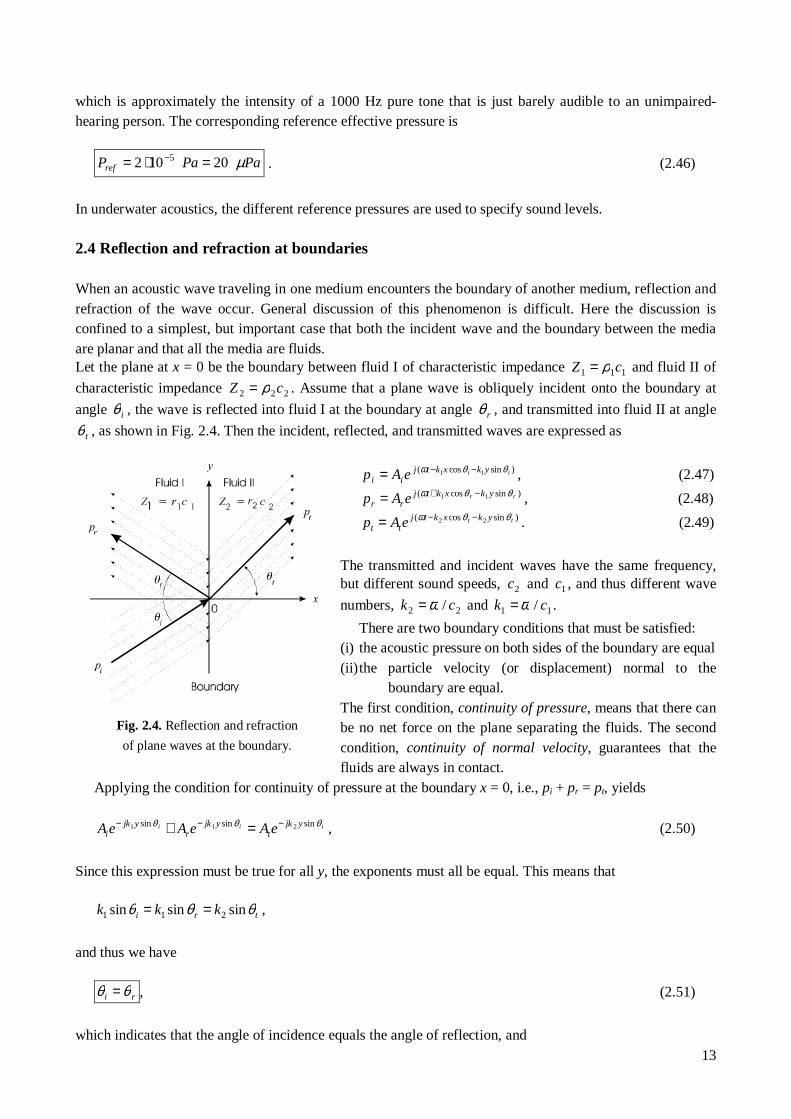
In underwater acoustics, the different reference pressures are used to specify sound levels. 2.4 Reflection and refraction at boundaries When an acoustic wave traveling in one medium encounters the boundary of another medium, reflection and refraction of the wave occur. General discussion of this phenomenon is difficult. Here the discussion is confined to a simplest, but important case that both the incident wave and the boundary between the media are planar and that all the media are fluids. Let the plane at x = 0 be the boundary between fluid I of characteristic impedance 111 cZ ρ= and fluid II of

characteristic impedance 222 cZ ρ= . Assume that a plane wave is obliquely incident onto the boundary at

angle iθ , the wave is reflected into fluid I at the boundary at angle rθ , and transmitted into fluid II at angle

tθ , as shown in Fig. 2.4. Then the incident, reflected, and transmitted waves are expressed as

)sincos( 11 ii ykxktjii eAp θθω −−= , (2.47)

)sincos( 11 rr ykxktjrr eAp θθω −+= , (2.48)

)sincos( 22 tt ykxktjtt eAp θθω −−= . (2.49)

The transmitted and incident waves have the same frequency, but different sound speeds, 2c and 1c , and thus different wave

numbers, 22 / ck ω= and 11 / ck ω= .

There are two boundary conditions that must be satisfied: (i) the acoustic pressure on both sides of the boundary are equal (ii) the particle velocity (or displacement) normal to the

boundary are equal. The first condition, continuity of pressure, means that there can be no net force on the plane separating the fluids. The second condition, continuity of normal velocity, guarantees that the fluids are always in contact.

Applying the condition for continuity of pressure at the boundary x = 0, i.e., pi + pr = pt, yields

tii yjkt

yjkr

yjki eAeAeA θθθ sinsinsin 211 −−− =+ , (2.50)

Since this expression must be true for all y, the exponents must all be equal. This means that tri kkk θθθ sinsinsin 211 == ,

and thus we have ri θθ = , (2.51)

which indicates that the angle of incidence equals the angle of reflection, and

Fig. 2.4. Reflection and refraction

of plane waves at the boundary.

14

21

sinsin

ccti θθ = , (2.52)

a statement of Snell’s law. Using the condition for continuity of the normal particle velocity at the boundary, vix + vrx = vtx, gives ttrrii vvv θθθ coscoscos =+ . (2.53)

Considering the relations 1Zpv ii = , 1Zpv rr −= , 2Zpv tt = , and ri θθ = , Eq. (2.53) becomes

( ) tti

ri c

A

cAA θ

ρρθ

coscos

2211

=− . (2.54)

Combining Eqs. (2.50) and (2.54), we obtain

ti

ti

i

r

cc

cc

A

AR

θρθρθρθρ

coscos

coscos

1122

1122

+−

== , (2.55)

which is defined as pressure reflection coefficient and

ti

i

i

t

cc

c

A

AT

θρθρθρ

coscos

cos2

1122

22

+== , (2.56)

which is defined as pressure transmission coefficient. From Eqs. (2.55) and (2.56), it is easy to find 1+R = T. From Snell’s law, we have

itt c

c θθθ 2

2

1

22 sin1sin1cos ���

����

�−=−= . (2.57)

It is important to note three implications of Eq. (2.57) (i) If 21 cc > , tθ is real and less than the angle of incidence. A transmitted beam exists in the second

medium and this beam is bent toward the normal to the boundary for all angles of incidence. (ii) If 21 cc < and ci θθ < where cθ is the critical angle given by

���

����

�=

2

1arcsinc

ccθ , (2.58)

tθ is again real but greater than the angle of incidence. A transmitted beam exists but the beam is bent

away from the normal to the boundary for all angles of incidence that are less than the critical angle. (iii) If 21 cc < and ci θθ > , tθcos is now pure imaginary. The incident wave is totally reflected. Intensity reflection and transmission coefficients are also often used in practice, and they are defined as

irI IIR = and itI IIT = , respectively, where iI , rI and tI are the intensities of the incident, reflected, and transmitted waves. The intensity reflection and transmission coefficients can be derived from the corresponding pressure coefficients,

15

2

RI

IR

i

rI == , (2.59)

and

2

22

11

cos

cosT

c

c

I

IT

i

t

i

tI θρ

θρ== . (2.60)

2.5 Standing waves A. Reflection of plane wave at a flat rigid boundary Consider the case in Fig. 2.4 where the boundary is rigid. In this case, the plane wave is completely reflected, and no energy is transmitted into medium II. Therefore, we have ri AA = , (2.61)

and the resulting wave in the 0≤x space is the sum of the incident and reflected waves,

ri ppp +=

)sinsin()coscos(2 11 iii yktxkA θωθ −= . (2.62)

For the normal incidence ( 0=iθ ) the equation becomes

)sin()cos(2 1 txkAp i ω= . (2.63)

The solution can be interpreted in two different but equivalent ways: (i) the interference of two waves of equal amplitude and wavelength traveling in opposite directions, and (ii) a waveform does not propagate, instead remains stationary. Therefore, such a wave is called a standing wave and is mathematically characterized by an amplitude that depends on the position along the propagation direction. A representative standing wave is shown in Fig. 2.5 where the pressure magnitude at various positions is plotted. The positions of zero pressure are called nodes and the positions of maximum pressure are called antinodes. The distance between the nodes is half wavelength 2/λ .

Fig. 2.5. Standing wave plotted

in terms of the variation range

of pressure magnitude as a

function of position.

16

B. Standing waves in the rectangular cavity Consider a rectangular cavity of dimensions xL , yL , zL , as shown in Fig. 2.6. This box could represent a

reverberant room or auditorium, a simple model of a concert hall, or any other rectangular space that has few windows or other openings and fairly rigid walls.

Fig. 2.6. The rectangular cavity

Assume that all surfaces of the cavity are perfectly rigid so that 0ˆ =⋅ vn at all boundaries. Then 0ˆ =∇⋅ pn

and thus

00

=��

���

�

∂∂=�

�

���

�

∂∂

== xLxx x

p

x

p; 0

0

=���

����

�

∂∂=��

�

����

�

∂∂

== yLyyy

p

y

p; 0

0

=��

���

�

∂∂=�

�

���

�

∂∂

== zLzz z

p

z

p (2.64)

Since acoustic energy can not escape from a closed cavity with rigid boundaries, appropriate solutions of the wave equation are standing waves. Substitution of

tjezZyYxXtzyxp ω)()()(),,,( = (2.65)

into the wave equation and separation of variables results in the sets of equations

022

2

=���

����

�+

∂∂

Xkx

Xx ; 02

2

2

=���

����

�+

∂∂

Yky

Yy ; 02

2

2

=���

����

�+

∂∂

Zkz

Zz (2.66)

where the separation constants must be related by

2222zyx kkkk ++= . (2.67)

Application of the boundary conditions in Eq. (2.64) shows that cosines are appropriate solutions, and Eq. (2.65) becomes

( ) ( ) ( ) tjznymxllmnlmn

lmnezkykxkAtzyxp ωcoscoscos),,,( = , (2.68)

where xxl Llk π= , ⋅⋅⋅= ,2,1,0l

yym Lmk π= , ⋅⋅⋅= ,2,1,0m (2.69)

zzn Lnk π= , ⋅⋅⋅= ,2,1,0n

17

Thus, the allowed frequencies of vibration, cklmn =ω or πω 2lmnlmnf = , are quantized,

222

���

����

�+

��

�

�

��

�

�+��

�

����

�==

zyxlmn L

n

L

m

L

lcck

πππω , or 222

2 ���

����

�+

��

�

�

��

�

�+��

�

����

�=

zyxlmn L

n

L

m

L

lcf (2.70)

which are determined by the cavity's dimensions xL , yL , zL with combinations of l, m, n.

Eq. (2.68) shows a series of discrete functions. These functions are called eigenfunctions, or normal modes, or resonance modes. Associated with each of the solutions is a unique frequency known as eigenfrequency, or normal mode frequency, or resonance frequency, determined by Eq. (2.70). The form in Eq. (2.68) gives three-dimensional standing waves in the cavity with nodal planes parallel to the walls. Between these nodal

planes the pressure varies sinusoidally, with pressure within a given loop in phase, with adjacent loops �180 out of phase. 2.6. Ray acoustics (geometric acoustics) Ray theory, although approximate, can give fairly good prediction to experimental measurements in reverberant rooms. Here the ray theory is very briefly introduced. In the real world, instead of plane waves, we find sound beams whose cross-sectional area and directions of propagation may change as the beams traverse the medium. In such circumstances, we frequently find it useful to think of rays rather than waves. A ray can be defined as a line everywhere perpendicular to the surfaces of constant phase (Fig. 2.7). Its usefulness lies in the intuitive feeling, mathematically justified under certain conditions, that energy is carried along a ray. In many cases, especially where c is a function of space or where the wave is restricted to a limited solid angle (such as the beams of sound from a highly directional source), description in terms of rays is much easier than wave fronts. However, rays are not exact replacements for waves but only approximations that are valid under certain rather restrictive conditions. The methods of treating reflection and refraction (Snell’s law) of plane waves apply to the propagation of rays. Fig. 2.8 shows an example of how the rays from a point source propagate in a rectangular room.

Fig. 2.7. Rays at a surface of equal phase. Fig. 2.8. Rays from a point source and their propagation.

18

3. Room acoustics Up to now quite a little knowledge has been presented about fundamentals of acoustics which is intended to establish a foundation that is enough for serving room acoustics. This section is going to present the room acoustics that is directly related with this project course of adaptive signal processing. 3.1. Sound in rooms Rooms that are either big or small are the necessary space for our living, working, entertaining, etc. Lots and lots of activities like conferences, concerts, sports events, and so on, happen in rooms. Perhaps we have such experience that the same speeches can feel very different when they are given in a concert hall, in a big conference room, in a classroom, in the rooms with a same size but different walls. Therefore, the shapes, dimensions and wall's surface structure of rooms have effect on sounds. How these affect sound is the subject of room acoustics.

Fig. 3.1. A process of sound generation and perception in a reverberant room.

A. Direct sound and reverberant sound Using ray model we can intuitively and approximately explain the sound process happening in a room. Assume that the speaker is approximated as a point source that generates spherical waves. The rays from the source travel outward in the diverging direction. At each encounter with the boundaries of the room, the rays are partly absorbed and partly reflected. Another assumption is that the listener is thought of as a small receiver (microphone). When the speaker makes a sound in a room, the sound then perceived by a listener or a microphone consists of the sound coming directly from the source (e.g., Ray D in Fig. 3.1) plus the sounds reflected or scattered by the walls (e.g., Rays 1R , 2R and 3R in Fig. 3.1) and by objects in the room. The

sound directly coming from the source is called direct sound, and the sound having undergone one or more reflections is called reverberant sound. For an impulse source the reverberant sound corresponds to a series of echoes. B. Anechoic chambers, reverberant chambers and reverberant rooms If the direct sound wave predominates almost everywhere, the room is anechoic (echo-free); rooms so designed are anechoic chambers. When the rooms are designed so that the reverberant wave predominates

19

overwhelmingly, they are called reverberant chambers. The rooms in which we are living are neither anechoic nor reverberant chambers, but the rooms in between and with certain reverberant effects; they are called reverberant or live rooms. C. Impulse response of a reverberant room Let us go back to the situation in Fig. 3.1. Also let a loudspeaker substitute the speaker that can make an impulse sound, and a microphone substitute the listener that perceives the sound in the reverberant room. A typical, representative measurement can look like that in Fig. 3.2, which was shown at the beginning of the acoustics session. The first impulse to the microphone is the direct sound, the second impulse that is smaller is the first reflection from the surface closest to the microphone, the third, the forth and the others are all the reflected sounds from the first or multiple reflections. The reflected sounds become smaller and smaller because they have more encounters with the surfaces and thus get absorption by the surface. As the more time has elapsed, the more reflected rays reach the microphone. Therefore, the impulses come closer and closer in time, i.e., the interval between the adjacent impulses gets smaller and smaller until they become diffused so that the sound throughout the room is well blended. This sound process may vary from room to room, depending on the acoustic properties of the rooms. To specify the acoustic property of a room, one important acoustic parameter is always used that is the reverberation time, defined as the time required for the sound pressure to drop 60 dB from the initial level, which will be presented in detail in the following section.

Fig. 3.2. Impulse response of a rectangular room.

What will happen if a source is turned on and continuously operates in a room? Experiments have shown that in this case the acoustic intensity at any point in the room builds up to higher values that would exist if the source were operated in open air, the gain in intensity often being greater than tenfold. In other words, the sound grows up in the room. For any given enclosure (or room) this gain is nearly proportional to the reverberation time. Therefore, a long reverberation time is desirable if a weak source of sound is to be audible everywhere in the room. If the source is shut off, the reception of direct sound ceases after a short time interval t = r/c, where r is the distance from the source to the point of observation and c is the speed of sound in air. The reflected waves continue to be received as succession of arrivals of decreasing intensity. The presence of this reverberant acoustic energy tends to mask the immediate recognition of any new sound, unless sufficient time has elapsed for the reverberation to fall down some 5 to 10 dB below its initial level. Since the reverberation time is a direct measure of the persistence of such sounds, it is obvious that a short

20

reverberation time is desirable to minimize masking effects. The choice of the best reverberation time for a particular room must, therefore, be a compromise. D. A simple model for the growth of sound in a room When a source of sound is started in a reverberant room, reflections at the walls produce a sound energy distribution that becomes more and more uniform with increasing time. Ultimately, except close to the source or to the absorbing surfaces, this energy distribution may be assumed to be completely uniform and to have essentially random local directions of flow. This is well known Sabine theory. Under this assumption, let the acoustic energy density E be uniform throughout the room with a volume of V. The rate at which the energy falls on a unit area of the wall can be found to be

4

Ec

dt

dE = , (3.1)

where c is the sound speed. If it is assumed that, at any point within the room, energy is arriving and departing along individual ray paths and that the rays have random phases at the point, then the energy density E is the sum over all rays of the energy densities mE of the individual rays. Supposing that the mth

ray has effective pressure emP , we have )/( 20

2 cPE emm ρ= , and thus

2

0

2

20

2

c

P

c

P

E ermem

ρρ==

�, (3.2)

where �=m

emer PP 22 is the spatially averaged effective pressure amplitude of the reverberant sound field.

If the total sound absorption of the room is A, then it follows from Eq. (3.1) that the rate at which energy is being absorbed by all surfaces is

EAc

4. (3.3)

Note that A has a unit of square meters and often given in metric sabin ( 2m ) or English sabin ( 2ft ).

According to the energy conservation, the rate of absorbed sound energy ( 4AcE ) plus the rate of growing

sound energy ( dtdEV ) throughout the interior of the room must equal the rate of energy W produced by the

sound source(s). From this, we obtain a fundamental differential equation that governs the growth of sound energy in a live room,

Wdt

dEVE

Ac =+4

. (3.4)

If the sound source is switched on at t = 0, solution of this differential equation and use of Eq. (3.2) yields

��

����

����

�−−=

Eer t

t

A

cWtP exp1

4)( 02 ρ

, (3.5)

where

Ac

VtE

4= (3.6)

is the time constant governing the growth of the acoustic energy in the room. If A (the total sound absorption) is small and the Et is large, a relative long time will be required for the effective pressure

amplitude and energy density E to approach the ultimate values of

21

A

cWPer

02 4)(

ρ=∞ and

Ac

WE

4)( =∞ (3.7)

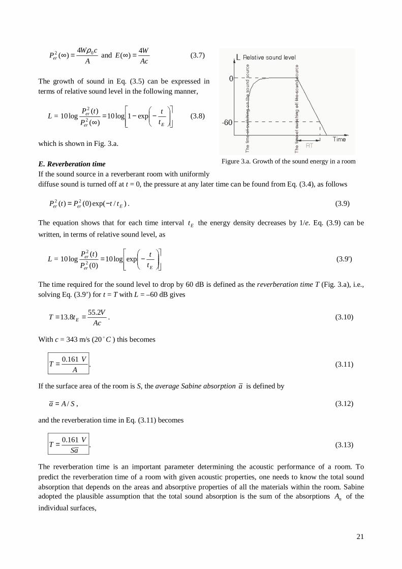
The growth of sound in Eq. (3.5) can be expressed in terms of relative sound level in the following manner,

L =

�

��

����

����

�−−=

∞ Eer

er

t

t

P

tPexp1log10

)(

)(log10

2

2

(3.8)

which is shown in Fig. 3.a. E. Reverberation time If the sound source in a reverberant room with uniformly diffuse sound is turned off at t = 0, the pressure at any later time can be found from Eq. (3.4), as follows

)/exp()0()( 22Eerer ttPtP −= . (3.9)

The equation shows that for each time interval Et the energy density decreases by 1/e. Eq. (3.9) can be

written, in terms of relative sound level, as

L =

�

��

����

����

�−=

Eer

er

t

t

P

tPexplog10

)0(

)(log10

2

2

(3.9')

The time required for the sound level to drop by 60 dB is defined as the reverberation time T (Fig. 3.a), i.e., solving Eq. (3.9’ ) for t = T with L = –60 dB gives

Ac

VtT E

2.558.13 == . (3.10)

With c = 343 m/s (20 C� ) this becomes

A

VT

161.0= . (3.11)

If the surface area of the room is S, the average Sabine absorption a is defined by SAa /= , (3.12)

and the reverberation time in Eq. (3.11) becomes

aS

VT

161.0= . (3.13)

The reverberation time is an important parameter determining the acoustic performance of a room. To predict the reverberation time of a room with given acoustic properties, one needs to know the total sound absorption that depends on the areas and absorptive properties of all the materials within the room. Sabine adopted the plausible assumption that the total sound absorption is the sum of the absorptions nA of the

individual surfaces,

Figure 3.a. Growth of the sound energy in a room

22

�� ==n

nnn

n aSAA , (3.14)

where na is the Sabine absorptivity of the nth surface nS . Thus, the average Sabine absorptivity becomes

�=n

nnaSS

a1

. (3.15)

Each na is to be evaluated from standardized measurements on a sample of the material in a reverberant

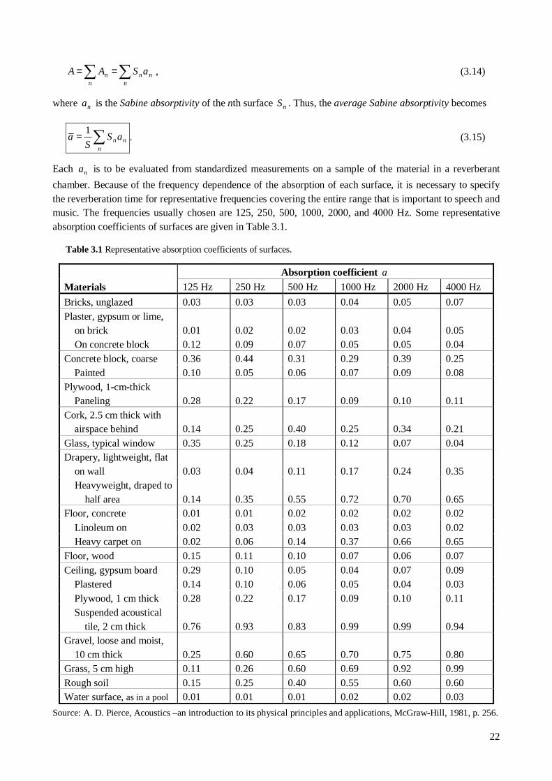
chamber. Because of the frequency dependence of the absorption of each surface, it is necessary to specify the reverberation time for representative frequencies covering the entire range that is important to speech and music. The frequencies usually chosen are 125, 250, 500, 1000, 2000, and 4000 Hz. Some representative absorption coefficients of surfaces are given in Table 3.1. Table 3.1 Representative absorption coefficients of surfaces.

Absorption coefficient a

Materials 125 Hz 250 Hz 500 Hz 1000 Hz 2000 Hz 4000 Hz

Bricks, unglazed 0.03 0.03 0.03 0.04 0.05 0.07 Plaster, gypsum or lime, on brick

0.01

0.02

0.02

0.03

0.04

0.05

On concrete block 0.12 0.09 0.07 0.05 0.05 0.04 Concrete block, coarse 0.36 0.44 0.31 0.29 0.39 0.25 Painted 0.10 0.05 0.06 0.07 0.09 0.08 Plywood, 1-cm-thick Paneling

0.28

0.22

0.17

0.09

0.10

0.11

Cork, 2.5 cm thick with airspace behind

0.14

0.25

0.40

0.25

0.34

0.21

Glass, typical window 0.35 0.25 0.18 0.12 0.07 0.04 Drapery, lightweight, flat on wall

0.03

0.04

0.11

0.17

0.24

0.35

Heavyweight, draped to half area

0.14

0.35

0.55

0.72

0.70

0.65

Floor, concrete 0.01 0.01 0.02 0.02 0.02 0.02 Linoleum on 0.02 0.03 0.03 0.03 0.03 0.02 Heavy carpet on 0.02 0.06 0.14 0.37 0.66 0.65 Floor, wood 0.15 0.11 0.10 0.07 0.06 0.07 Ceiling, gypsum board 0.29 0.10 0.05 0.04 0.07 0.09 Plastered 0.14 0.10 0.06 0.05 0.04 0.03 Plywood, 1 cm thick 0.28 0.22 0.17 0.09 0.10 0.11 Suspended acoustical tile, 2 cm thick

0.76

0.93

0.83

0.99

0.99

0.94

Gravel, loose and moist, 10 cm thick

0.25

0.60

0.65

0.70

0.75

0.80

Grass, 5 cm high 0.11 0.26 0.60 0.69 0.92 0.99 Rough soil 0.15 0.25 0.40 0.55 0.60 0.60 Water surface, as in a pool 0.01 0.01 0.01 0.02 0.02 0.03

Source: A. D. Pierce, Acoustics –an introduction to its physical principles and applications, McGraw-Hill, 1981, p. 256.

23

Conventionally, when the term reverberation time is used without specification of any particular frequency, it is generally understood to refer to the frequency of 500 Hz. An example is given in Fig. 3.3, showing measurements of reverberation times at three different frequencies, 125, 500 and 2500 Hz.

Fig. 3.3. Measurements of reverberation times at three different frequencies, 125, 500 and 2500 Hz.

Criteria for what constitutes good acoustics for rooms intended for specified purposes have been extensively developed since a long ago. The reverberation time plays a central role in the quantitative formulation of some of the simpler criteria, like the example shown in Fig. 3.4.

Fig. 3.4. Optimum midfrequency (500 to 1000 Hz) reverberation times for fully occupied rooms versus volume (from

A. D. Pierce, Acoustics – an introduction to its physical principles and applications, McGraw-Hill, 1981, p. 271).

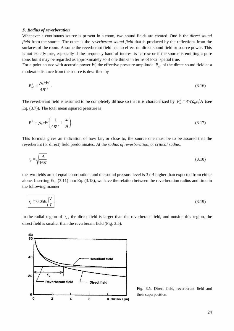
24

F. Radius of reverberation Whenever a continuous source is present in a room, two sound fields are created. One is the direct sound field from the source. The other is the reverberant sound field that is produced by the reflections from the surfaces of the room. Assume the reverberant field has no effect on direct sound field or source power. This is not exactly true, especially if the frequency band of interest is narrow or if the source is emitting a pure tone, but it may be regarded as approximately so if one thinks in terms of local spatial true. For a point source with acoustic power W, the effective pressure amplitude edP of the direct sound field at a

moderate distance from the source is described by

2

02

4 r

cWPed π

ρ= . (3.16)

The reverberant field is assumed to be completely diffuse so that it is characterized by AcWPer 02 4 ρ= (see

Eq. (3.7)). The total mean squared pressure is

��

���

� +=Ar

cWP4

4

120

2

πρ . (3.17)

This formula gives an indication of how far, or close to, the source one must be to be assured that the reverberant (or direct) field predominates. At the radius of reverberation, or critical radius,

π16

Arr = (3.18)

the two fields are of equal contribution, and the sound pressure level is 3 dB higher than expected from either alone. Inserting Eq. (3.11) into Eq. (3.18), we have the relation between the reverberation radius and time in the following manner

T

Vrr 056.0= . (3.19)

In the radial region of rr , the direct field is larger than the reverberant field, and outside this region, the

direct field is smaller than the reverberant field (Fig. 3.5).

Fig. 3.5. Direct field, reverberant field and

their superposition.

25

3.2. Standing waves and normal modes in rooms In the previous section 3.1, based on ray acoustics, we have derived formulas for determining the reverberation time, the average Sabine absorption, reverberation radius, and the others. Ray acoustics, however, does not provide a complete theory of the behavior of sound in an enclosure. A more adequate approach must be based directly on wave theory. The wave equation has been solved (at least approximately) for simple enclosures (such as rectangular and hemispherical spaces) and new concepts have emerged from examining the transient and steady-state behaviors of sound in such enclosures. Even in complicated enclosures for which the wave equation cannot be solved, the theory has been used to supplement and extend results provided by ray-acoustic methods.

Fig. 3.6. Five different normal modes of pressure field in a rectangular room with dimension of 6x4 2m .

A. Normal modes and eigenfrequencies in a rectangular room As presented in Sect. 2.5, the solution of the wave equation in a lossless, rigid-wall, rectangular cavity of dimensions of xL , yL , zL , results in the normal modes

tfj

zyxlmnlmn

lmnezL

ny

L

mx

L

lAtzyxp ππππ 2coscoscos),,,( ��

�

����

���

�

�

��

�

����

����

�= , (3.20)

which are a series of discrete functions, each with its own eigenfrequency expressed by

26

222

2 ���

����

�+

��

�

�

��

�

�+��

�

����

�=

zyxlmn L

n

L

m

L

lcf . (3.21)

The eigenfrequencies are completely determined by the nature of the room. The modes are labeled by the integer set (l, m, n). If all the integers are not zero, the normal mode is termed oblique. If one of the integers is zero, the mode is termed tangential because the propagation vector of the wave is parallel to one pair of the room surfaces. If two of the integers is zero, the mode is termed axial because the propagation vector of the wave is parallel to one of the surface axes. Fig. 3.6 illustrates some normal modes in a rectangular room 6x4 m. B. Frequency distribution of room resonaces, and high frequency approximation Knowledge of the eigenfrequencies of a room is essential to a complete understanding of its acoustic properties. When a source is present, the room will respond strongly to those sounds having frequencies in the immediate vicinity of any of these eigenfrequencies. It is just this characteristic that affects the output of a loudspeaker as measured in a reverberant room and causes the distorted results of the loudspeaker’s properties. Each standing wave has its own eigenfrequency and thus its own particular spatial pattern of nodes and antinodes. In effect, superposition of the characteristics of the room with those of any sound source present results in the fluctuations in sound pressure that vary with position and frequency. Therefore, as a microphone is moved from point to another, or as the frequency of the source is varied, the fluctuations may completely conceal the true output characteristics of the source. It is for this reason that measurements of the response curves of loudspeakers should be carried out either in the open air or in anechoic chamber. If the absorption coefficient is greater than 0.99, the reverberant field is negligible compared to the direct wave. Each of the individual standing waves of a cavity can be excited to its fullest extent by a sound source located in regions where the particular standing wave pattern has a pressure antinode (recall Sect. 2.5). Observing the normal modes in Eq. (3.20), we see that the pressure amplitudes of all patterns of standing waves in a rectangular cavity are maximized in the corners of the room. Therefore, if the source is at the corner of such a room, it will possible for it to excite every allowed normal mode to its fullest extent. Correspondingly, if a microphone is located in the corner of the room, it will measure the peak sound pressure of every normal mode that has been excited. By contrast, when a source is located in a region where a particular normal mode has a pressure node, that mode will be excited only weakly. For instance, if a loudspeaker is located in the center of a rectangular room, only those modes having even numbers simultaneously for l, m, and n will be excited ( about 1 mode in 10) as the driving frequency is slowly varied from low to high frequencies. An example, which is the second example presented at the beginning of the Introduction, is to be looked into in more detail. A rectangular room has a dimension of 3.12x4.69x6.24. The normal modes with corresponding normal mode frequencies below 100 Hz are given in Table 3.2. A loudspeaker is positioned at one corner of the room, and the microphone is located in a diagonally opposite corner. In this circumstance, the measurement was carried out by slowly increasing the frequency supplied by the loudspeaker from 20 to 100 Hz and simultaneously recording the output of the microphone. The recorded result is shown in Fig. 3.7 in solid line. In the figure the output of the loudspeaker measured in an anechoic chamber is given in dashed line. In comparison, the influence of the room is apparent. When either the loudspeaker or microphone is positioned in the center of the room, only those peaks corresponding to the (0, 0, 2), (0, 2, 0) and (0, 2, 2) modes would be observed below 100 Hz.

27

Table 3.2. Normal mode frequencies below 100 Hz for a rectangular room of 3.12x4.69x6.24 with c = 345 m/s.

l m n f (Hz) l m n f (Hz)

0 0 1 27.5 1 0 2 77.5 0 1 0 36.6 0 2 1 78.5 0 1 1 45.9 0 0 3 82.5 1 0 0 55.0 1 1 2 86.5 0 0 2 55.0 0 1 3 90.2 1 0 1 61.5 0 2 2 91.5 0 1 2 66.0 1 2 0 91.5 1 1 0 66.0 1 2 1 95.5 1 1 1 71.5 1 0 3 99.0 0 2 0 73.2

Fig. 3.7. Normal mode response of a rectangular room 3.12x4.69 x 6.24 m at low frequencies.

Modal density is defined as the number of room normal modes per unit frequency bandwidth. Let N(f) denote the number of room normal modes whose eigenfrequencies are less than a given value of f. In the case of a rectangular room with dimensions of xL , yL , zL , the total number of modes N(f) can be calculated using

Eq. (3.21) with ff lmn ≤ ,

8

1

843

4)(

23

+��

���

�+��

���

�+��

���

�≈c

fL

c

fS

c

fVfN

π, (3.22)

where V is the volume of the room, S= )(4 xzzyyx LLLLLL ++ is the total surface area and

L= )(2 zyx LLL ++ is the total length of all the edges in the room. The number of normal modes in a

frequency bandwidth f∆ and centered at frequency f, denoted by N∆ , can be estimated as [ ] fdffdN ∆)( .

Thus, the average number of modes per unit frequency bandwidth (modal density) is

c

Lf

c

Sf

c

V

df

fdN

84

4)(2

23

++= π. (3.23)

28

When the room dimensions are large compared with wavelength, the first term predominates. Taking the leading term yields the form of modal density that is commonly used in the high frequency range, the number of normal modes in a frequency bandwidth f∆ becomes

N∆ ffc

Vf

df

fdN ∆=∆≈ 23

4)( π. (3.24)

This shows that the number of normal modes in a given frequency band width f∆ increases rapidly as the

center frequency of the band (or the size of the room) is increased. As a result, the responses of the standing waves will overlap more and more at higher frequencies so that the response of the room will become quite smooth with increasing frequency. Since the standing wave pattern corresponding to each eigenfrequency is in general associated with some particular set of direction cosines, any increase in N∆ indicates an increase in the randomness of directions of the associated waves. This is supported by the observation that reverberation equations based on a diffuse sound field, such as Eq. (3.11), are in better agreement with experiments at high frequencies. The response of a room is observed to become less uniform with increasing its symmetry because the number of degenerate modes having different (l, m, n) but the same natural frequency is increased. From Eq. (3.24) we can estimate the average frequency spacing modef∆ (in Hz) of eigenfrequencies in the frequency bandwidth f∆ in the following manner,

2

3

mode4 Vf

c

N

ff

π=

∆∆

=∆ . (3.25)

Whenever the source driving frequency f is sufficiently close to the eigenfrequency f(n), a resonance is apparent. The nth normal mode becomes dominant as )(nff → . The bandwidth of the resonance peak can

be found approximately to be

Tt

fE

res ππ 2

8.13

2

1 ==∆ . (3.26)

If the average spacing modef∆ between the resonance peaks is of the order of or less than, say 5.2resf∆ , the

resonance peaks may be regarded as a smoothed-out continuum. Since the average spacing modef∆ decrease

with increasing frequency, there is a frequency Schf , called Schroeder cutoff frequency, below which

modef∆ < 5.2resf∆ is not satisfied and above which it is. This frequency is identified, from Eqs. (3.25) and

(3.26), as

V

Tcf Sch 2.55

5 3

= . (3.27)

This, with c = 340 m/s, becomes

V

Tf Sch 1900≈ . (3.28)

The Schroeder rule says that above the Schroeder cutoff frequency a sum over mode indices can be approximated by an integral. In other words above Schf the normal modes may be regarded as a smoothed-

out continuum. In this case, room acoustics should be treated from the statistical aspects. Deviation of acoustic quantities from the averages predicted by the Sabine model are frequently given a statistical interpretation.