Embed Size (px)
Citation preview
Projection Methods forClustering and
Semi-supervisedClassification
David Paul Hofmeyr, B.Sc. (Hons), M.Sc., M.Res.
Submitted for the degree of Doctor of Philosophyat Lancaster University
November, 2015

Abstract
This thesis focuses on data projection methods for the purposes of cluster-ing and semi-supervised classification, with a primary focus on clustering.A number of contributions are presented which address this problem in aprincipled manner; using projection pursuit formulations to identify sub-spaces which contain useful information for the clustering task. Projectionmethods are extremely useful in high dimensional applications, and situa-tions in which the data contain irrelevant dimensions which can be counter-informative for the clustering task. The final contribution addresses highdimensionality in the context of a data stream. Data streams and high dimen-sionality have been identified as two of the key challenges in data clustering.
The first piece of work is motivated by identifying the minimum densityhyperplane separator in the finite sample setting. This objective is directlyrelated to the problem of discovering clusters defined as connected regionsof high data density, which is a widely adopted definition in non-parametricstatistics and machine learning. A thorough investigation into the theoreticalaspects of this method, as well as the practical task of solving the associatedoptimisation problem efficiently is presented. The proposed methodology isapplied to both clustering and semi-supervised classification problems, andis shown to reliably find low density hyperplane separators in both contexts.
The second and third contributions focus on a different approach to clus-tering based on graph cuts. The minimum normalised graph cut objective hasgained considerable attention as relaxations of the objective have been devel-oped, which make them solvable for reasonably well sized problems. Thishas been adopted by the highly popular spectral clustering methods. Thesecond piece of work focuses on identifying the optimal subspace in whichto perform spectral clustering, by minimising the second eigenvalue of thegraph Laplacian for a graph defined over the data within that subspace. Arigorous treatment of this objective is presented, and an algorithm is pro-posed for its optimisation. An approximation method is proposed whichallows this method to be applied to much larger problems than would other-wise be possible. An extension of this work deals with the spectral projectionpursuit method for semi-supervised classification.
iii
The third body of work looks at minimising the normalised graph cut us-ing hyperplane separators. This formulation allows for the exact normalisedcut to be computed, rather than the spectral relaxation. It also allows for acomputationally efficient method for optimisation. The asymptotic propertiesof the normalised cut based on a hyperplane separator are investigated, andshown to have similarities with the clustering objective based on low den-sity separation. In fact, both the methods in the second and third works areshown to be connected with the first, in that all three have the same solutionasymptotically, as their relative scaling parameters are reduced to zero.
The final body of work addresses both problems of high dimensionalityand incremental clustering in a data stream context. A principled statisticalframework is adopted, in which clustering by low density separation againbecomes the focal objective. A divisive hierarchical clustering model is pro-posed, using a collection of low density hyperplanes. The adopted frame-work provides well founded methodology for determining the number ofclusters automatically, and also identifying changes in the data stream whichare relevant to the clustering objective. It is apparent that no existing methodscan make both of these claims.

Acknowledgements
To begin with I would like to thank my supervisors. Nicos, your enthusi-asm for the work we have done during my thesis has been a great source ofmotivation. Idris, you have always provided an encouraging and somehowcalming perspective on my research, and research in general. I have learneda lot from both of you, and I am extremely grateful. Thanks too for puttingup with me these past few years, I know that my repeatedly ignoring youradvice and comments can’t always have gone unnoticed.
I would also like to thank both the EPSRC and the Oppenheimer Memo-rial Trust for providing funding during my Ph.D.
To Jon, Idris and Kevin; the STOR-i doctoral training centre has beenthe ideal environment in which to do my Ph.D. You’ve outdone yourselves.Thank you.
To the friends I have made during my time here in Lancaster, in particu-lar my year group in STOR-i, you’ve always provided sufficient distractionsfrom work to make the Ph.D seem manageable, even when things have beendifficult. The whole process could not have been nearly as enjoyable withoutyou guys.
To my family, you have been continuous sources of support and encour-agement and I will forever be grateful. The admittedly too infrequent chats,though perhaps seemingly just chats, have sometimes felt like the only thingkeeping me going.
Finally, to Aeysha, your love and encouragement has been constant and Idon’t know if I could have managed without that. There are a lot of things Icould say, but I think what captures it well (at least it does for me), is that youstubbornly refuse to ever accept that I could have shortcomings; you alwaysmanage to find some other explanation for why I could be struggling. Thankyou, for your oblivion, for everything.
v

Abstract
vi

Declaration
I declare that the work in this thesis has been done by myself and has notbeen submitted elsewhere for the award of any other degree.
David Paul Hofmeyr
vii

Abstract
viii

Contents
Abstract iii
Acknowledgements v
Declaration vii
Thesis Details xiii
List of Figures xiii
List of Tables xvii
1 Introduction 11 Clustering . . . . . . . . . . . . . . . . . . . . . . . . . . . . . . . 4
1.1 Centroid-Based Clustering . . . . . . . . . . . . . . . . . 51.2 Connectivity-Based Clustering . . . . . . . . . . . . . . . 61.3 Graph Partitioning Based Clustering . . . . . . . . . . . 81.4 Density-Based Clustering . . . . . . . . . . . . . . . . . . 101.5 Model-Based Clustering . . . . . . . . . . . . . . . . . . . 11
2 Semi-supervised Classification . . . . . . . . . . . . . . . . . . . 122.1 Low Density Separation Methods . . . . . . . . . . . . . 132.2 Graph Partition Based Methods . . . . . . . . . . . . . . 14
3 Challenges in Data Clustering . . . . . . . . . . . . . . . . . . . 153.1 High Dimensionality . . . . . . . . . . . . . . . . . . . . 153.2 Data Streams . . . . . . . . . . . . . . . . . . . . . . . . . 17
4 Focus of Thesis . . . . . . . . . . . . . . . . . . . . . . . . . . . . 194.1 Contributions . . . . . . . . . . . . . . . . . . . . . . . . . 19
2 Minimum Density Hyperplane: An Unsupervised and Semi-supervisedClassifier 211 Introduction . . . . . . . . . . . . . . . . . . . . . . . . . . . . . . 222 Problem Formulation . . . . . . . . . . . . . . . . . . . . . . . . . 25
2.1 Clustering . . . . . . . . . . . . . . . . . . . . . . . . . . . 26
ix

Contents
2.2 Semi-Supervised Classification . . . . . . . . . . . . . . . 303 Connection to Maximum Margin Hyperplanes . . . . . . . . . . 31
3.1 MDP2 for Clustering . . . . . . . . . . . . . . . . . . . . . 343.2 MDP2 for Semi-Supervised Classification . . . . . . . . . 35
4 Estimation of Minimum Hyperplanes . . . . . . . . . . . . . . . 364.1 Computational Complexity . . . . . . . . . . . . . . . . . 38
5 Experimental Results . . . . . . . . . . . . . . . . . . . . . . . . . 385.1 Clustering . . . . . . . . . . . . . . . . . . . . . . . . . . . 395.2 Semi-Supervised Classification . . . . . . . . . . . . . . . 455.3 Summary of Experimental Results . . . . . . . . . . . . . 48
6 Conclusions . . . . . . . . . . . . . . . . . . . . . . . . . . . . . . 49Appendix. Proof of Theorem 1 . . . . . . . . . . . . . . . . . . . . . . 507 Proof of Theorem 1 . . . . . . . . . . . . . . . . . . . . . . . . . . 50
3 Projection Pursuit Based on Spectral Connectivity 54
A. Minimum Spectral Connectivity Projection Pursuit for Unsuper-vised Classification 551 Introduction . . . . . . . . . . . . . . . . . . . . . . . . . . . . . . 552 Related Work . . . . . . . . . . . . . . . . . . . . . . . . . . . . . 583 Background on Spectral Clustering . . . . . . . . . . . . . . . . . 594 Projection Pursuit for Spectral Connectivity . . . . . . . . . . . . 61
4.1 Continuity and Differentiability . . . . . . . . . . . . . . 624.2 Minimising λ2(L(θθθ)) and λ2(Lnorm(θθθ)). . . . . . . . . . . 674.3 Computing Similarities . . . . . . . . . . . . . . . . . . . 694.4 Correlated and Orthogonal Projections . . . . . . . . . . 71
5 Connection with Maximal Margin Hyperplanes . . . . . . . . . 746 Speeding up Computation using Microclusters . . . . . . . . . . 797 Experimental Results . . . . . . . . . . . . . . . . . . . . . . . . . 86
7.1 Details of Implementation . . . . . . . . . . . . . . . . . . 877.2 Clustering Results . . . . . . . . . . . . . . . . . . . . . . 897.3 Summarising Clustering Performance . . . . . . . . . . . 937.4 Sensitivity Analysis . . . . . . . . . . . . . . . . . . . . . 95
8 Conclusions . . . . . . . . . . . . . . . . . . . . . . . . . . . . . . 98Appendix. Derivatives . . . . . . . . . . . . . . . . . . . . . . . . . . . 100
B. Semi-supervised Spectral Connectivity Projection Pursuit 1031 Introduction . . . . . . . . . . . . . . . . . . . . . . . . . . . . . . 1032 Spectral Clustering . . . . . . . . . . . . . . . . . . . . . . . . . . 1053 Methodology . . . . . . . . . . . . . . . . . . . . . . . . . . . . . 105
3.1 Computational Complexity . . . . . . . . . . . . . . . . . 1104 Experiments . . . . . . . . . . . . . . . . . . . . . . . . . . . . . . 1115 Conclusions . . . . . . . . . . . . . . . . . . . . . . . . . . . . . . 112
x
Contents
Appendix. Proofs . . . . . . . . . . . . . . . . . . . . . . . . . . . . . . 114
4 Clustering by Minimum Cut Hyperplanes 1181 Introduction . . . . . . . . . . . . . . . . . . . . . . . . . . . . . . 1182 Problem Formulation . . . . . . . . . . . . . . . . . . . . . . . . . 120
2.1 Background on Normalised Graph Cuts . . . . . . . . . 1212.2 Normalised Cuts Across Hyperplanes . . . . . . . . . . . 1212.3 Connection with Maximum Margin Hyperplanes . . . . 126
3 Methodology . . . . . . . . . . . . . . . . . . . . . . . . . . . . . 1283.1 Optimal NCut of the Marginal Data Set v · X . . . . . . 1283.2 Optimising Φ(v|X ) . . . . . . . . . . . . . . . . . . . . . 1303.3 Beyond Bi-partitioning . . . . . . . . . . . . . . . . . . . . 133
4 Experimental Results . . . . . . . . . . . . . . . . . . . . . . . . . 1344.1 Parameter Settings for NCutH and NCutH0 . . . . . . . 1354.2 Clustering Performance . . . . . . . . . . . . . . . . . . . 1364.3 Run Time Analysis . . . . . . . . . . . . . . . . . . . . . . 138
5 Conclusion . . . . . . . . . . . . . . . . . . . . . . . . . . . . . . . 141Appendix. Proofs . . . . . . . . . . . . . . . . . . . . . . . . . . . . . . 142
5 Divisive Clustering of High Dimensional Data Streams 1501 Introduction . . . . . . . . . . . . . . . . . . . . . . . . . . . . . . 1502 Related Work . . . . . . . . . . . . . . . . . . . . . . . . . . . . . 1533 Problem Description . . . . . . . . . . . . . . . . . . . . . . . . . 1544 Methodology . . . . . . . . . . . . . . . . . . . . . . . . . . . . . 157
4.1 Learning High Variance Projections . . . . . . . . . . . . 1574.2 Splitting Based on a Projected Sample . . . . . . . . . . . 1584.3 Handling Population Drift . . . . . . . . . . . . . . . . . 164
5 The HSDC Algorithm . . . . . . . . . . . . . . . . . . . . . . . . 1665.1 Computational Complexity . . . . . . . . . . . . . . . . . 167
6 Experimental Results . . . . . . . . . . . . . . . . . . . . . . . . . 1686.1 Simulations . . . . . . . . . . . . . . . . . . . . . . . . . . 1706.2 Publicly Available Data Sets . . . . . . . . . . . . . . . . 1756.3 Discussion of Experimental Results . . . . . . . . . . . . 178
7 Conclusion . . . . . . . . . . . . . . . . . . . . . . . . . . . . . . . 179Appendix. Proofs . . . . . . . . . . . . . . . . . . . . . . . . . . . . . . 180
6 Conclusion 1841 Summary of Contributions . . . . . . . . . . . . . . . . . . . . . 1842 An Experimental Comparison of the Contributions . . . . . . . 187
2.1 Projected Divisive Clustering . . . . . . . . . . . . . . . . 1872.2 Large Margin Clustering . . . . . . . . . . . . . . . . . . 1882.3 A Summary of Clustering Performance . . . . . . . . . . 1892.4 Semi-supervised Classification . . . . . . . . . . . . . . . 192
xi

Contents
3 Possible Extensions and Future Work . . . . . . . . . . . . . . . 195
Bibliography 197References . . . . . . . . . . . . . . . . . . . . . . . . . . . . . . . . . . 198
xii
Thesis Details
Thesis Title: Projection Methods for Clustering and Semi-supervisedClassification
Ph.D. Student: David Paul HofmeyrSupervisors: Dr. Nicos Pavlidis, Lancaster University
Prof. Idris Eckley, Lancaster UniversityExaminers: Dr. Ludger Evers, University of Glasgow
Dr. Chris Sherlock, Lancaster University
The main body of this thesis consist of the following papers.
• Chapter 2 has been submitted for publication as; Pavlidis, N. G., Hofmeyr,D. P and Tasoulis, S. K. “Minimum Density Hyperplanes,” 2016.
• Chapter 3 A. has been submitted for publication as; Hofmeyr, D. P,Pavlidis, N. G. and Eckley, I. “Minimum Spectral Connectivity Projec-tion Pursuit for Unsupervised Classification," 2016.
• Chapter 3 B. has been accepted for publication as; Hofmeyr, D. P. andPavlidis, N. G. “Semi-supervised Spectral Connectivity Projection Pur-suit", PRASA-RobMech International Conference, 2015.
• Chapter 4 has been submitted for publication as; Hofmeyr, D. P. “Clus-tering by Minimum Cut Hyperplanes", 2016.
• Chapter 5 has been accepted for publication as; Hofmeyr, D. P., Pavlidis,N. G. and Eckley, I. “Divisive Clustering of High Dimensional DataStreams," Statistics and Computing, issn: 0960-3174, doi: 10.1007/s11222-015-9597-y, Springer, 2015.
The majority of works involved collaboration with others, most notably mysupervisors. In the case of Chapter 2, Nicos Pavlidis took an especially sig-nificant role.
xiii

Thesis Details
xiv
List of Figures
2.1 Binary partitions induced by 100 MDHs estimated throughSQP and MDP2 . . . . . . . . . . . . . . . . . . . . . . . . . . . . 29
2.2 Impact of choice of α on minimum density hyperplane. . . . . 422.3 Evolution of the minimum density hyperplane through con-
secutive iterations. . . . . . . . . . . . . . . . . . . . . . . . . . . 432.4 Performance and Regret Distributions for all Methods Consid-
ered . . . . . . . . . . . . . . . . . . . . . . . . . . . . . . . . . . . 462.5 Classification error for different number of labelled examples
for datasets with two clusters. . . . . . . . . . . . . . . . . . . . . 472.6 Classification error for different numbers of labelled examples
over all pairwise combinations of classes. . . . . . . . . . . . . . 482.7 Two dimensional illustration of Lemma 8 . . . . . . . . . . . . . 51
3.1 Effect of T∆ on Distances and Similarities. . . . . . . . . . . . . . 723.2 Two dimensional projections of optical recognition of hand-
written digits dataset arising from the minimisation of λ2(L(θθθ)),for different values of β. In addition, the initialisation throughPCA is also shown. The top row of plots shows the true clus-ters, while the bottom row shows resulting bi-partitions. . . . 73
3.3 Large Euclidean separation of the yeast cell cycle dataset. Theleft plots show the result from a 2 dimensional projection pur-suit using the proposed method. The middle plots show the1 dimensional projection pursuit result. The right plots showthe result of the maximum margin clustering method of Zhanget al. (2009). . . . . . . . . . . . . . . . . . . . . . . . . . . . . . . 79
3.4 Approximation Error Plots for S1 data set. . . . . . . . . . . . . 853.5 Box plots of relative purity with additional red dots to indicate
means. Methods are ordered with decreasing mean value. . . 963.6 Box plots of relative V-measure with additional red dots to
indicate means. Methods are ordered with decreasing meanvalue. . . . . . . . . . . . . . . . . . . . . . . . . . . . . . . . . . 97
xv
List of Figures
3.7 Sensitivity analysis for varying σ. Standard Laplacian. Thex-axis contains the multiplication factor applied to the defaultscaling parameter used in the experiments. . . . . . . . . . . . 97
3.8 Sensitivity analysis for varying σ. Normalised Laplacian. Thex-axis contains the multiplication factor applied to the defaultscaling parameter used in the experiments. . . . . . . . . . . . 98
3.9 Sensitivity analysis for varying number of microclusters, K.Plots show median and interquartile ranges of performancemeasures from 30 datasets simulated from 50 dimensional Gaus-sian mixtures with 5 clusters and 1000 observations. . . . . . . 99
3.10 Sensitivity analysis for fixed number of microclusters, K =200, and varying number of data. Plots show median and in-terquartile ranges of performance measures from datasets sim-ulated from 50 dimensional Gaussian mixtures with 5 clustersand between 1000 and 10 000 observations. . . . . . . . . . . . . 100
3.11 Two projections, one admitting a separation of the classes (Left)and the other not (Right). . . . . . . . . . . . . . . . . . . . . . . 109
4.1 Optimal hyperplanes based on NCut (left) and RatioCut (right)from the same 100 initialisations . . . . . . . . . . . . . . . . . . 126
4.2 Regret distributions of Purity (top) and V-Measure (bottom)across all 15 benchmark data sets. . . . . . . . . . . . . . . . . . 140
4.3 Run time analysis from Gaussian mixtures. The plot shows themedians and interquartile ranges from 50 replications for eachvalue of n. The number of clusters is fixed at 5. . . . . . . . . . 140
5.1 Different changes in distribution and their impact on the clus-tering model. Red lines indicate necessity of model revision.Green lines indicate changes which can be addressed by ex-tending the model without revision . . . . . . . . . . . . . . . . 165
5.2 Performance on Static Data Stream with 20 Classes in 500 Di-mensions . . . . . . . . . . . . . . . . . . . . . . . . . . . . . . . . 171
5.3 Clustering Performance. Static Environment with IrrelevantFeatures. 20 Classes in 100 Relevant and 100 Irrelevant Dimen-sions with Moderate Variability . . . . . . . . . . . . . . . . . . . 172
5.4 Clustering Performance. Decreasing Classes. 500 Dimensions . 1745.5 Clustering Performance. Increasing Classes. 500 Dimensions . 1755.6 Clustering Performance. Distribution Overhaul. 20 Classes in
500 Dimensions . . . . . . . . . . . . . . . . . . . . . . . . . . . . 1765.7 Class Proportions of Forest Cover Type . . . . . . . . . . . . . . 1775.8 Clustering Performance. Forest Cover Type Data . . . . . . . . . 1775.9 Clustering Performance. Gas Sensor Array Data . . . . . . . . . 178
xvi

List of Figures
6.1 Box plots of relative purity with additional red dots to indicatemeans. Methods are ordered with decreasing mean value. . . 192
6.2 Box plots of relative V-measure with additional red dots toindicate means. Methods are ordered with decreasing meanvalue. . . . . . . . . . . . . . . . . . . . . . . . . . . . . . . . . . 193
6.3 Box plots of regret based on purity with additional red dotsto indicate means. Methods are ordered with increasing meanvalue. . . . . . . . . . . . . . . . . . . . . . . . . . . . . . . . . . 194
6.4 Box plots of regret based on V-measure with additional reddots to indicate means. Methods are ordered with increasingmean value. . . . . . . . . . . . . . . . . . . . . . . . . . . . . . . 195
xvii

List of Figures
xviii

List of Tables
2.1 Details of Benchmark Data Sets . . . . . . . . . . . . . . . . . . 392.2 Performance on the task of binary partitioning. (Ties in best
performance were resolved by considering more decimal places) 45
3.1 Purity results for spectral clustering using the standard Lapla-cian, L. Average performance from 30 runs on each dataset,with standard deviation as subscript. The highest average per-formance in each case is highlighted in bold. . . . . . . . . . . 90
3.2 V-measure results for spectral clustering using the standardLaplacian, L. Average performance from 30 runs on each dataset,with standard deviation as subscript. The highest average per-formance in each case is highlighted in bold. . . . . . . . . . . . 91
3.3 Purity results for spectral clustering using the normalised Lapla-cian, Lnorm. Average performance from 30 runs on each dataset,with standard deviation as subscript. The highest average per-formance in each case is highlighted in bold. . . . . . . . . . . 92
3.4 V-measure results for spectral clustering using the normalisedLaplacian, Lnorm. Average performance from 30 runs on eachdataset, with standard deviation as subscript. The highest av-erage performance in each case is highlighted in bold. . . . . . 92
3.5 Purity results for large margin clustering. Average perfor-mance from 30 runs on each dataset, with standard deviationas subscript. The highest average performance in each case ishighlighted in bold. . . . . . . . . . . . . . . . . . . . . . . . . . 93
3.6 V-measure results for large margin clustering. Average perfor-mance from 30 runs on each dataset, with standard deviationas subscript. The highest average performance in each case ishighlighted in bold. . . . . . . . . . . . . . . . . . . . . . . . . . 94
3.7 UCIMLR Classification Data Sets. Average Accuracy (%) over10 Splits. . . . . . . . . . . . . . . . . . . . . . . . . . . . . . . . . 113
3.8 SSC Benchmark Data Sets. Average Accuracy (%) over 12 Splits. 113
xix
List of Tables
4.1 Details of Benchmark Data Sets . . . . . . . . . . . . . . . . . . 1354.2 100 × Purity on Benchmark Data Sets. Highest Performance
Highlighted in Bold. . . . . . . . . . . . . . . . . . . . . . . . . . 1384.3 100 × V-Measure on Benchmark Data Sets. Highest Perfor-
mance Highlighted in Bold. . . . . . . . . . . . . . . . . . . . . 1394.4 Run Time on Benchmark Data Sets (in Seconds) . . . . . . . . . 141
5.1 Clustering Performance. Static environments. . . . . . . . . . . 1715.2 Clustering Performance. Static environments with irrelevant
features. . . . . . . . . . . . . . . . . . . . . . . . . . . . . . . . . 1735.3 Clustering Performance. Drifting environments. . . . . . . . . . 176
6.1 A Comparison of the Performance of Proposed Methods forProjected Divisive Clustering. The Table Shows 100 × Purityon Benchmark Data Sets. Highest Performance in Each Case isHighlighted in Bold. . . . . . . . . . . . . . . . . . . . . . . . . . 188
6.2 A Comparison of the Performance of Proposed Methods forLarge Margin Clustering. The Table Shows 100 × V-Measureon Benchmark Data Sets. Highest Performance in Each Case isHighlighted in Bold. . . . . . . . . . . . . . . . . . . . . . . . . . 189
6.3 A Comparison of the Performance of Proposed Methods forLarge Margin Clustering. The Table Shows 100 × Purity onBenchmark Data Sets. Highest Performance in Each Case isHighlighted in Bold. . . . . . . . . . . . . . . . . . . . . . . . . . 190
6.4 A Comparison of the Performance of Proposed Methods forLarge Margin Clustering. The Table Shows 100 × V-Measureon Benchmark Data Sets. Highest Performance in Each Case isHighlighted in Bold. . . . . . . . . . . . . . . . . . . . . . . . . . 191
6.5 A Comparison of the Proposed Methods for Semi-supervisedClassification applied to UCI Machine Learning Repository Clas-sification Data Sets. Average Accuracy (%) over 10 Splits. . . . . 193
6.6 A Comparison of the Proposed Methods for Semi-supervisedClassification applied to Benchmark Data Sets taken from Chap-elle et al. (2006b). Average Accuracy (%) over 12 Splits. . . . . . 194
xx
Chapter 1
Introduction
The problem of identifying groups of related objects is one of the fundamen-tal tasks in knowledge discovery from data. This problem has been exten-sively studied in the literature on statistics, machine learning, data miningand pattern recognition because of the numerous applications in summarisa-tion, learning and segmentation (Jain and Dubes, 1988; Aggarwal and Reddy,2013). Such applications include,
• Engineering: In manufacturing, group technology seeks to identify sim-ilar items so that manufacturing and design concepts can be borrowed,thus speeding up the manufacturing lifecycle of emerging items (Phamand Afify, 2007). In radar signal analysis, the direction of arrival ofpulses is crucial for object locating, however the sheer density of sig-nals creates a computational challenge which is mitigated by identi-fying groups of pulses (Zhu et al., 2010). Outlier rejection deals withseparating a single group of objects from remaining nuisance observa-tions which do not fit within the group’s context, this has applicationsin robotics in the form of consistent hypothesis identification (Olson etal., 2005).
• Computer Science: Web mining deals with organising the billions ofweb pages on the internet, so that queries can be handled efficiently.Grouping similar web objects, often by textual content, significantlyaids this challenging task (Chen and Chau, 2004). Computer vision andimage segmentation tasks require identifying different planar rangesin an image, which may be achieved by grouping small sections of animage, or sequence of images, to determine separate planes and usingtheir respective orientation and geometry (Frigui and Krishnapuram,1999).
• Life Sciences: In the study of spatial population genetics, tracing geo-
1
Chapter 1. Introduction
graphical ancestries can be aided by finding similar allele groups fromspatially recorded genetic information (Rosenberg et al., 2002). Group-ing lifestyle factors which have higher combined prevalence in indi-viduals suffering certain diseases than would be predicted given theirindividual prevalence has use in preventative medicine (Schuit et al.,2002).
• Social Sciences: Person perception, in the field of psychology, looksat the different mental processes used to form impressions of peo-ple. Grouping people based on their perceptions of archetypal life fig-ures has been useful in identifying psychopathologies (Rosenberg et al.,1996). The success of an education institution is predicated on both aca-demic performance and enrollment management. Grouping studentsbased on their persistence with academic courses can be useful in bothareas, especially for early identification of potential defectors (Luan,2002).
• Commerce: Market segmentation can be achieved by identifying groupsof related consumers or products (Punj and Stewart, 1983), and is a cen-tral feature in targeted marketing strategy. Outlier rejection, as in therobotics application, can also be used to identify fraudulent behaviourof consumers or organisations, comparing behavioural patterns withthe general behaviour of a group (Phua et al., 2010).
Broadly speaking the task of assigning a set of objects to groups may betermed classification (Jain and Dubes, 1988), and exists on three distinct levelsin terms of the assumed available information. In the machine learning lit-erature the amount of information available may be described by degrees ofsupervision for the learning task. On one end of the spectrum is the fully su-pervised classification task, in which the true groupings of all data used in thelearning phase of the task are known. An inductive model is then built whichcan be used to predict the groupings of future data. It is the fully supervisedtask which is commonly given the name “classification". On the other end ofthe spectrum lies unsupervised classification. In this context there is no ex-plicit information regarding how data should be grouped. The relationshipsbetween data must therefore be learned by other means. In this context anymodel which assigns groupings to data is used only within the context of thedata used to build the model, and is not used to predict the groupings offuture unseen data. Between these extremes lies semi-supervised classifica-tion. The motivation for semi-supervised classification can be seen as follows.When using a (supervised) classification model to predict the groupings ofnew data, there is an implicit assumption that the nature of those new data,in terms of their grouping tendencies, is somewhat related to the nature ofthe data used in building the model. If this assumption is true, then utilis-
2
ing whatever information about the new data is available, within the contextof all the data, may be useful in determining the groups to which they be-long. Semi-supervised classification is extremely useful in situations whereidentifying the true group labels for data is expensive. In such situations thenumber of labelled data may be small, and making inference or predictionfrom a (supervised) classification model can be unreliable, and the predictiontask can be substantially aided by utilising every bit of available information.
This thesis focuses on the latter two, with a primary focus on the unsu-pervised problem. Semi-supervised classification is treated within the sameframework, as an extension of the unsupervised case. Utilising informationabout data which does not explicitly determine their groups is therefore thecentral feature of the work presented. Throughout the remainder it is as-sumed that a data set is described by a fixed set of features, each taking a(real) numerical value. Data may therefore be thought of as occupying a vec-tor space defined over the real numbers in which the number of dimensionsis equal to the number of features describing the data.
A common assumption when data arise from multiple groups, or classes,is that the data tend to contain multiple clusters, and that objects withinthe same cluster are more likely to represent the same group. In the con-text of semi-supervised classification this is referred to as the cluster assump-tion (Chapelle and Zien, 2005), and in the unsupervised case leads to the fieldof cluster analysis. Cluster analysis has a very rich history, and remains oneof the most active and important areas of research in fields relying on theanalysis of data. The term cluster analysis, or simply clustering, is often usedto refer to the task of unsupervised classification.
Accepting the cluster assumption immediately begs the question of whatconstitutes a cluster of data, and numerous definitions have been proposed,each leading to hosts of methods for identifying clusters which adhere tothese definitions. Arguably the single common concept underpinning all ofthese, though, is that the spatial relationships between data contain usefulinformation for determining clusters. The spatial relationships in this con-text are defined by the topological structure bestowed on the vector spacecontaining the data, usually via the Euclidean (or L2) norm, although othermetrics may be used.
This thesis is motivated by two of the key challenges associated with dataclustering, both from practical and theoretical points of view. The principalmotivation comes from the problem of dimension reduction. Dimension re-duction forms a crucial part of the analysis of data which are either highdimensional, i.e., data containing a very large number of features, or datawhich contain features, or combinations of features, that may be irrelevantor even counter-informative for identifying clusters. A number of contri-
3
Chapter 1. Introduction
butions are presented which address this problem in a principled manner;using projection-pursuit formulations to identify subspaces which containuseful information for the clustering task. A secondary motivation arisesfrom the challenge associated with clustering data incrementally, where dataare received sequentially in a data stream. The final contribution of this thesisaddresses both challenges, and proposes a method for clustering high dimen-sional data streams within a principled statistical framework. Further detailsof these contributions are given at the end of this chapter.
The remainder of this chapter is organised as follows. In Section 1 a numberof cluster definitions are explored, as well as some important methods forfinding clusters which fit within their respective definitions. In Section 2 adiscussion of semi-supervised classification methods will be presented, withparticular attention to those adhering to the cluster assumption. Followingthat, in Section 3 some fundamental challenges associated with clusteringmethods from practical, theoretical and philosophical perspectives will bepresented. The focus of the remaining thesis will then be outlined in Sec-tion 4.
Neither of Sections 1 and 2 is intended to be a comprehensive account ofthe entire literature on these problems, but rather provides a representativecross section of concepts and methods which are either highly influential orof relevance in the remaining thesis. Each subsequent chapter will containits own review, documenting existing approaches which are of particularimportance for the context of that chapter.
1 Clustering
This section is dedicated to the discussion of existing methods for clustering.Important concepts and methods in the clustering literature are discussed un-der the headings relating to different definitions of what constitutes a clus-ter. Clustering methods can also be split between two distinct approachesto model structure. Hierarchical clustering models are nested sequences ofpartitions (Jain and Dubes, 1988) and may be further categorised into divi-sive and agglomerative clustering. In divisive clustering, beginning with theentire data set being a cluster, clusters are recursively partitioned until a stop-ping criterion is met. Conversely, agglomerative clustering begins with everydatum in its own cluster, and repeatedly merges clusters until all data arecontained in a single cluster. Partitional clustering models instead directlyassign data to their final clusters in a single step. Partitional methods mayalso be referred to as generating a flat clustering. The focus of this section willbe more strongly motivated by the concept of what constitutes a cluster, thanby the model structure in which the clusters reside. The reason being that
4
1. Clustering
the philosophy behind a particular approach to establishing or identifying re-lated groups of objects is much more closely related to the group definitionsthan their representation.
1.1 Centroid-Based Clustering
Centroid-based clustering defines clusters in relation to single representativepoints (centroids). Data are thought to collect around these points, formingclusters. Models derived from these clustering methods may be summarisedby a set of centroids, and data are classified based on which centroid is near-est to them (Leisch, 2006). This approach generates a partitional clusteringmodel.
Formally, the clustering task may be stated in relation to the followingoptimisation problem,
minC∈F k
n
∑i=1
minc∈C
f (d(xi, c)). (1.1)
Here the xi, i = 1, ..., n represent the data points and the set C is the setof centroids over which the optimisation takes place. The set F representsthe collection of feasible centroid values. The function f : R+ → R+ isnon-decreasing, and operates on the distances between the data and theirassociated centroids, via the distance metric d(·, ·). In these approaches thenumber of centroids, and therefore clusters, k, is chosen by the user.
The k-means clustering method is seen as one of the simplest and mostclassical approaches to data clustering (Jain, 2010) and remains one of themost widely used in practice, largely due to its simplicity (Aggarwal andReddy, 2013). In the k-means approach the optimal clustering model is de-fined as the set of k centroids which minimises the sum of the squared Eu-clidean distances between each datum and its cluster centroid. In terms of theabove optimisation, (1.1), one therefore has f (x) = x2 and d(x, y) = ‖x− y‖2.The centroids are essentially unconstrained, and so the set F is given by thewhole space from which the data set arose. It is straightforward to showthat with this objective, the centroids for the optimal model are defined asthe means of the data assigned to each cluster. A simple iterative algorithmwas proposed by Lloyd (1957, 1982). The algorithm is initialised with a setof k potential centroids. It then alternates between assigning the data to theirnearest centroid, and then updating the centroids by giving them the valueequal to the mean of the data assigned to them. This is repeated until thesolution converges.
Solving the objective in (1.1), where instead the L1 norm is used and sim-ple distances, rather than squared distances as in k-means, determine thefunction f leads to the k-medians clustering problem (Bradley et al., 1997).
5
Chapter 1. Introduction
The structure of the algorithm for solving this problem is essentially the sameas for the k-means objective. Both k-means and k-medians have worst casecomputational complexity which is non-polynomial in general, even for find-ing local optima, however most implementations have an empirical run timewhich is of O(nkD), where D the number of dimensions.
In k-medoids clustering, the centroids are selected from the data set itself.Therefore the set F is given by x1, ..., xn. This is especially useful when theobjects being clustered may not permit a reasonable interpretation of mean ormedian (Aggarwal and Reddy, 2013). While the number of iterations is oftenmore than is required for solving either k-means or k-medians (Aggarwal andReddy, 2013), this approach does have the benefit that distance calculationscan be recycled since many of the pairwise inter-distance calculations willhave been performed in previous iterations.
The above methods represent three of the fundamental centroid-basedclustering methods, largely due to the fact that the centroids admit closedform solutions, making them especially attractive from a computational pointof view. The problem formulation, however, allows for any general distancefunction to be used, and modern optimisation techniques have allowed forthese to be implemented practically (Leisch, 2006).
Centroid-based clustering methods benefit from their ease of implemen-tation, and fast computation in most practical examples. They also have closeconnections with model-based clustering, for example the k-means solutioncan be seen as an approximation of the Gaussian Mixture Model solution fora fixed number of clusters, and isotropic covariance matrices. The funda-mental limitations of these approaches are the low flexibility of cluster shape,since cluster boundaries are given by the Voronoi tesselation of the centroids,and the fact that the number of clusters must be prespecified.
1.2 Connectivity-Based Clustering
Unlike in centroid-based clustering, the pairwise distances between data pointsare the driving force in connectivity-based clustering. The term connectivityrefers to the algorithmic approach of merging data, or clusters of data alreadydetermined, until all data are connected as a single cluster. This generates anagglomerative model, and different levels in the hierarchy provide the clus-tering result at different granularity/scale.
Within single-linkage clustering, at each step in the agglomerative proce-dure precisely two clusters (which may be singletons) are merged. The pairselected for merging is that which has the minimum distance between theclusters, based on the standard metric extension to sets. That is, the smallestpairwise distance between them. Formally, if C1, ..., Ck represent the clusters atiteration n− k + 1, then at iteration n− k + 2 clusters Ci and Cj are replaced
6
1. Clustering
with Ci ∪ Cj, where i, j minimise
minl,m⊂1,...,k
minx∈Cl ,y∈Cm
d(x, y). (1.2)
This approach is called single linkage as only a single pair of data belong-ing to the two clusters being merged need to be close together, i.e., a singlelink of short distance must exist. Sibson (1973) developed a quadratic time,linear storage algorithm for generating this hierarchical model. Both of thesecomplexities have been shown to be optimal for this problem.
In complete-linkage clustering on the other hand, the pair of clustersmerged is the pair between which the largest distance is minimal. In otherwords, (1.2) is replaced with,
minl,m⊂1,...,k
maxx∈Cl ,y∈Cm
d(x, y). (1.3)
A similar algorithm to that of Sibson (1973) for single linkage clustering wasproposed by Defays (1977), which again has quadratic time complexity in thenumber of data. This has been shown to be the optimal complexity for thecomplete linkage problem as well.
Other analogous models have been proposed, wherein the only differenceis the rule for selecting the next pair of clusters to be merged. An exampleof this is the average linkage approach, or Unweighted Pair Group Methodwith Arithmetic mean (UPGMA), proposed by Sokal and Michener (1958).A quadratic time algorithm for the method was later developed by Murtaghand Raftery (1984).
Alternative to the strategy of merging a single pair of clusters repeatedlyis an approach in which all pairs of clusters satisfying a connectedness cri-terion are merged. Weakening the connectedness criterion, for example byincreasing the minimum distance required to satisfy connectedness, leads tomore and more clusters being merged. If all pairwise distances are different,then it is clear that this approach can be made equivalent to the single-linkageapproach above. Within this formulation, at each iteration the clusters can beinterpreted as the connected components of a graph defined over the clus-ters present at the previous iteration. An edge is present in the graph if andonly if the two corresponding clusters are merged at the current iteration.Graph based methods will be discussed in greater detail below, where moregeneral graphs, i.e., with edges weights assuming continuous values, will bepermitted.
An advantage of connectivity based methods is that they admit clustersof arbitrary shape, and utilise information in the data set at a local level. Inpractice, though, the single linkage approach has been criticised for its ten-dency to emphasise elongated clusters caused by the chaining effect inherentin its formulation. The computational complexity of these methods limitsthem to data sets of only moderate size.
7
Chapter 1. Introduction
1.3 Graph Partitioning Based Clustering
Graph partitioning approaches for clustering draw on the wealth of existinggraph theoretic methods to produce clustering models. In order to do so, agraph must be defined which is relevant to the clustering task. Certain datastructures, such as networks, immediately lend themselves to graph formu-lations, however it is possible to define a graph which has useful propertiesfor clustering an arbitrary set of objects provided a quantitative measure ofsimilarity between pairs of objects is available. Consider a complete graph inwhich each object is designated a vertex, and edge weights take values equalto the similarity between their adjacent vertices. Then subgraphs containingcomparatively high edge weights correspond to collections of objects whichare mostly similar, and can therefore be interpreted as clusters. Alternatively,assigning edge weights equal to the distance between the adjacent verticesmeans that subgraphs with relatively low edge weights may correspond toclusters of data which are close together. Some notions of optimality in thiscontext have been introduced, and will be discussed below.
Using graph cuts is an intuitive way of obtaining clusters of similar ob-jects. A graph cut is given by the sum of the edge weights connecting dif-ferent components of a partition of the graph. If the edges represent thesimilarities between data, then minimising the cut will form a clustering ofa data set in which the data in different clusters have low similarity. Graphcuts can be usefully formulated using an affinity matrix, A ∈ Rn×n : Ai,j =similarity(xi, xj). For a partition of the data set into clusters C1, ..., Ck, thegraph cut may then be given by
Cut(C1, ..., Ck) =12
k
∑l=1
∑xi∈Cl ,xj 6∈Cl
Aij. (1.4)
Minimising this graph cut objective has been found to often result in verysmall clusters (von Luxburg, 2007). This is because the number of edgesbeing “broken" by the cut is equal to (|C|(N − |C|)), which is minimised ifeither |C| = 1 or |C| = N − 1. Forcing clusters to be above a specific size, ornormalising the graph cut objective to emphasise more balanced partitionsmakes the problem NP-hard (Wagner and Wagner, 1993). It can be shownthat two popular normalisations of the graph cut objective, namely RatioCutand normalised cut (NCut), can be formulated under the following problemstructure,
minC1,...,Ck
trace(H>LH) (1.5a)
s.t. H>KH = I (1.5b)
Hij =
1/√
size(Cj), xi ∈ Cj
0, otherwise.(1.5c)
8
1. Clustering
The matrix L := D− A ∈ Rn×n is called the graph Laplacian, where D is thediagonal matrix with ii-th entry ∑n
j=1 Aij, and the matrix H ∈ Rn×k encodesthe cluster memberships for each of k clusters. For RatioCut, the size of acluster is measured by its cardinality, and the matrix K is simply the identity.For NCut, size is measured by the volume of a cluster, given by ∑xi∈C Dii, andK = D. Spectral methods can be used to find approximate solutions to thenormalised cut problem (Hagen and Kahng, 1992; Shi and Malik, 2000), inwhich the constraint on the matrix H given by (1.5c) is relaxed. The solutionin this case is given if the columns of H are replaced with the k smallesteigenvectors of L, or of D−1/2LD−1/2 in the case of NCut. However, in thiscase the clusters are not fully determined, and a second clustering step isperformed on the rows of H to determine the final clustering of the data.This leads to the popular spectral clustering algorithms (von Luxburg, 2007).A more detailed account of spectral clustering and normalised cuts is given inChapters 3 and 4. The second step in which the final clusters are determinedcan provide an alternative interpretation of spectral clustering, in which thematrix H represents a partial embedding of the data within a kernel space.In particular, if the clustering step is performed using k-means, then spectralclustering can be shown to be a special case of so-called kernel k-means(Dhillon et al., 2004).
An alternative approach to graph cuts uses minimum weight spanningtrees (MSTs). When edges correspond to the distance between the adjacentvertices, the MST gives the fully connected graph which contains the shortesttotal distance between the data. The edges in the MST are likely therefore tocontain the important connections between data within clusters. A theoremfrom Zahn (1971) shows that if a bi-partition of a data set attains the largestpossible distance between the two elements of the partition, based on theminimum pairwise distance between data, then the restriction of the MST toeach element in the partition remains connected, i.e., is a subtree. That is, ifC is the solution to
maxB⊂x1,...,xn
minx∈B,y 6∈B
d(x, y), (1.6)
then the subset of edges in the MST which connect elements of C is a con-nected subgraph. A direct consequence of this result is that by removingthe largest weighted edge from the MST, the remaining subgraphs define thetwo-way clustering of the data set which maximises the distance betweenthem. To generate a full clustering model, what remains is a method for re-moving the edges from the MST which are likely to exist between clusters,rather than within them. In the geometric minimum spanning tree cluster-ing method (Brandes et al., 2003) a performance measure is computed foreach clustering obtained by removing from the minimum spanning tree theedges with weight above a threshold. Since the tree has only n − 1 edges,where n is the size of the data set, only n − 1 such thresholds need to be
9
Chapter 1. Introduction
considered. The fuzzy C-means minimum spanning tree method (Foggia etal., 2007) instead clusters the edges based on their weights using the fuzzyC-means algorithm, and retains only those in the cluster of smaller edgeweights.
1.4 Density-Based Clustering
In density-based clustering, clusters are defined as regions of high data den-sity which are separated from other high density regions by a region of lowdata density. The density at a point may be related to the number of datafalling within a specified neighbourhood size or by using a smoother kernel-based estimate (Aggarwal and Reddy, 2013).
The DBSCAN clustering algorithm (Ester et al., 1996) uses the former ofthe above definitions. In this case high density points are those points withina specific distance of at least a chosen minimum number of other data. Eachhigh density point is then connected to all points lying within the specifieddistance, and sets of connected points are defined as clusters. Any pointwhich is not within the specified distance of at least one high density pointis interpreted as an outlier, not belonging to any cluster.
DBSCAN can be seen as approximating the level sets of a kernel densityestimate of the data distribution, where the uniform kernel is used. In thenon-parametric statistics literature, this method is often applied to a moregeneral density estimate (Azzalini and Torelli, 2007; Stuetzle and Nugent,2010). In this case clusters are defined as maximally connected componentsof the level set of a probability density function (Hartigan, 1975). The level setof a function is the subset of the function’s domain upon which the functionalvalue lies above a chosen threshold level. Formally, the level set of a functionf : X → R at level λ is defined as,
x ∈ X | f (x) ≥ λ. (1.7)
Computing the level sets of an unknown probability density directly is ex-tremely challenging even in moderate dimensions (Stuetzle and Nugent, 2010).Certain approaches approximate these level sets as the union of spheresaround those data at which the estimate of the density is above the thresh-old level (Cuevas and Fraiman, 1997; Rinaldo and Wasserman, 2010). Thismethod has compelling consistency properties (Rinaldo and Wasserman, 2010),in that these approximations form disjoint neighbourhoods of the true com-ponents of the level sets of the underlying density with high probability.However, in the clustering context it is only the groups of data occupyingthese components of the level sets which are of interest. Other methodstherefore attempt to connect data (i.e., assign them to the same cluster) byestablishing if there is a path between them lying completely within the levelset of the density (Azzalini and Torelli, 2007; Stuetzle and Nugent, 2010).
10
1. Clustering
Different interpretations of where the density is “high", i.e., using differ-ent threshold levels for the level set, gives rise to different clusterings, andusing this approach for a range of thresholds results in a hierarchical clus-tering model, known as the cluster tree. A more in depth account of density-based clustering, especially from the non-parametric statistical perspective isprovided in Chapters 2 and 5.
An alternative approach to density-based clustering is via a grid formula-tion. In this case it is the cells of a grid defined over the space occupied by thedata which undergoes clustering. In this case, the concept of adjacency hasa far more interpretable meaning, and so establishing connections betweengrid cells is less challenging than for data points. Here the grid cells contain-ing sufficiently many points are seen as high density cells, and adjacent highdensity cells are joined to produce clusters. The final clustering of the dataconnects data belonging to the same clusters of grid cells. An advantage ofthis approach is that they are at least theoretically applicable in high dimen-sional applications, because the lower dimensional grids define clusters onsubsets of the dimensions. Such a hierarchical grid structure, where the hi-erarchy is defined over the dimensions, can be seen in the STING clusteringmethod (Wang et al., 1997).
A major advantage of density-based clustering is that the number of clus-ters can be estimated automatically, and moreover they provide a naturalframework for handling outliers. In addition, they are well founded from astatistical perspective in that a feature of the underlying probability distri-bution is being estimated directly, and are capable of representing the fullunderlying distribution. From a computational point of view, in the generalcase density methods can be complex. These methods are also highly limitedin their applicability to higher dimensions, since the sparsity of data makesestimating the underlying density unreliable, and in grid-based approachesthe size of the grid grows exponentially with the number of dimensions.
1.5 Model-Based Clustering
Model-based clustering again assumes an underlying probability distributionhas generated the data. Unlike the non-parametric approach in the previoussubsection, however, the data are assumed to be a sample from a finite mix-ture distribution in which each component has a known parametric form.Formally, the data set is assumed to be a sample of realisations of a randomvariable X with density function f , where f may be expressed as,
f (x) =k
∑i=1
πi fi(x|θi). (1.8)
Here the π′is are the mixing proportions, i.e., ∑ki=1 πi = 1, πi > 0, and each fi is
a density function parameterised by θi. If all parameters of the mixture distri-
11
Chapter 1. Introduction
bution can be estimated, then data are classified according to which compo-nent in the mixture has the greatest posterior probability of having generatedit (Fraley and Raftery, 2002). In other words each datum is classified by,
Class(xj) = argmaxi∈1,...,kπi fi(xj|θi). (1.9)
In general all components are assumed to belong to the same family of dis-tributions, i.e., fi = f j ∀i, j, with the Gaussian mixture model being the mostcommon.
Both partitional and agglomerative clustering approaches have been ap-plied to this setting. In the partitional case (McLachlan and Basford, 1988;Celeux and Govaert, 1995), parameter estimation can be done using Expec-tation Maximisation for mixture models. The agglomerative method usesthe same algorithmic structure as connectivity based cluster, where in thiscase the criterion for merging two clusters is based on classification likeli-hood (Murtagh and Raftery, 1984; Banfield and Raftery, 1993).
Once a family of distributions has been chosen for the individual compo-nents in the mixture, methods can be further divided by how much freedomis allowed in the estimation of parameters. If parameter values are uncon-strained, then the number of parameters that need to be estimated can belarge, leading to computational issues. Moreover, the reliability in estimationcan be negatively affected if few data are used for each parameter, and inthe extreme case this approach can lead to a lack of identifiability. In theGaussian mixture case, constraints on the covariance matrices of the differ-ent components can be introduced; either forcing all covariances to be equalto the same scaled identity matrix, or allowing for an arbitrary covariancebut ensuring it is shared by all components (Friedman and Rubin, 1967). Amore general framework was given by Banfield and Raftery (1993) wherecovariances matrices are described by their eigen-decomposition and certainelements in this decomposition are fixed for all components, while others areallowed to vary.
Probably the most attractive feature of model based clustering is that theproblem of determining the number of clusters is stated within the thor-ough statistical framework of model selection, where measures such as theBayesian Information Criterion (Schwartz, 1978) can be used. The fundamen-tal limitation is that clusters should be describable by a known parametricdistribution, and also that all clusters should fall into the same family ofdistributions.
2 Semi-supervised Classification
In semi-supervised classification the true groupings, or class identities, ofsome of the data are known (labeled data) and the task is to assign the data
12
2. Semi-supervised Classification
whose classes are unknown (unlabeled data) to one of the classes definedwithin the labeled data. The motivation behind many approaches to solvingthis problem is the assumption that data which lie within the same clusterare likely to belong to the same class. One of the earliest approaches tosemi-supervised classification was based on this cluster assumption (Chap-elle et al., 2006b). In this section, a selection of cluster motivated semi-supervised classification methods will be discussed.
2.1 Low Density Separation Methods
If clusters are seen as regions of high data density which are separated byrelatively sparse regions, then an assumption equivalent to the cluster as-sumption is the so-called low density separation assumption: The boundaryseparating classes should lie in a low density region (Chapelle et al., 2006b).Many modern approaches to the semi-supervised classification problem fo-cus more on the low density separation assumption, and try to identify lowdensity regions which separate the known classes.
A common approach to determining the low density boundaries is throughSupport Vector Machines (Vapnik and Sterin, 1977). SVMs were originally de-signed for supervised classification, and are used to find the linear separator(hyperplane) which separates the classes and which attains the largest marginon the data, in other words the linear separator which is as far as possibleaway from its nearest datum. Kernel methods can be used to find non-linearseparators by implicitly embedding the data in a higher dimensional space.In semi-supervised classification, the Transductive SVM (TSVM) is the hy-perplane which separates the classes and attains the largest margin on boththe labeled and unlabeled data (Joachims, 2006). The corresponding optimi-sation problem is posed in the context of the standard SVM, except that theclass labels for the unlabeled data are treated as decision variables. Sincethe set of labels is discrete, this corresponds to a mixed integer quadraticprogramme, for which no efficient algorithms exist (Joachims, 2006).
Various authors have attempted to solve the problem exactly (Vapnik andSterin, 1977; Bennett and Demiriz, 1998), but this approach is limited to caseswith at most hundreds of unlabeled data points. The SVMlight approach pro-posed by Joachims (1999) does not find the global optimum, but can handleproblems with up to 100000 data. The method uses a local descent approachwhich iteratively swaps two labels assigned to unlabeled data. A similarapproach was proposed by Demiriz and Bennet (2000), which differs fromSVMlight in the number of labels and which selection of labels are swapped,as well as the heuristics used to avoid local optima (Joachims, 2006). Fi-nally De Bie and Cristianini (2004) used a convex relaxation via semi-definiteprogramming. Chapelle et al. (2006a) used a continuation approach to avoidlocal minima in the TSVM objective. In this approach a sequence of optimisa-
13
Chapter 1. Introduction
tion problems is solved, where each is initialised with the solution to the pre-vious probelm. In each the objective is convolved with a Gaussian smoothingkernel for a shrinking sequence of bandwidths. As the bandwidth decreasesthe objective function for the convolved problem becomes closer to the trueunderlying objective, and this procedure has the potential to find very goodsolutions.
The Low Density Separation (LDS) approach of Chapelle and Zien (2005)attempts to establish if unlabeled points can be connected to a labeled pointby a path of high density. A robust estimate of the lowest density point alongthe best path between pairs of data is used to establish a density sensitivedistance measure, which is then used to define a kernel used in the training ofa TSVM.
2.2 Graph Partition Based Methods
The graph formulation described in relation to clustering provides a conve-nient framework for incorporating additional information, such as knownclass labels as in semi-supervised classification. Since the graph may bedefined via edges taking values equal to the pairwise similarities betweendata, edges joining data known to belong to the same class can be assignedmaximum similarity, while edges between data known to belong to differ-ent classes may be assigned the minimum similarity value. Using a nor-malised cut technique would therefore tend to separate the classes in the la-beled data as well as connect unlabeled data which are similar to the knownclasses under the resulting clustering. This sort of approach has been imple-mented (Chen and Feng, 2012) in the related field of semi-supervised clustering;a problem in which no class labels are known but pairs of data may be knownto belong to the same class or not, thereby introducing constraints in the clus-tering formulation.
In the semi-supervised classification context, a number of approacheshave been proposed. Label Propagation uses an iterative procedure to propa-gate labels through a similarity graph (Bengio et al., 2006). A labelling vectoris updated by repeatedly multiplying by the normalised similarity matrixuntil convergence. The early algorithm by Zhu and Ghahramani (2002) hasbeen extended to allow for more general clusters and to improve the stabilityof the algorithm (Bengio et al., 2006), or by smoothing the actual labellingvector in an approach referred to as label spreading (Zhou et al., 2004).
In addition to these methods, some authors have combined the kernelbased classification objective with the spectral clustering objective to ob-tain so-called Laplacian Regularisation or Laplacian SVM (Sindhwani etal., 2006).
14
3. Challenges in Data Clustering
3 Challenges in Data Clustering
This section investigates two challenges associated with data clustering whichhave received considerable attention in the literature. Subection 3.1 looks atthe problem of partitioning data with a very large number of features, so-called high dimensional data. This is a fundamental challenge faced in a vari-ety of problems in data analysis, and extends beyond the obvious computa-tional difficulty associated with processing data objects of a much larger size.Subsection 3.2 covers the data stream paradigm. In a data stream environ-ment, the objects being partitioned arrive in sequence and cannot be storedin memory. The model used for assigning data to groups must therefore bebuilt incrementally.
3.1 High Dimensionality
The fundamental challenge, from a theoretical point of view, associated withanalysing high dimensional data is that data points become increasinglysparse as dimensionality increases (Steinbach et al., 2004). This concept ismost easily intuited using a grid-based representation. For a fixed numberof grid cells partitioning each dimension, the number of total grid cells inthe full dimensional space grows exponentially with the dimension. Unlessthe number of available data grows with at least the same rate, then for avery large number of dimensions the ratio of non-empty cells to empty cellsapproaches zero. The space is, in a sense, “almost everywhere" sparse.
From a practical point of view, one of the major challenges for datapartitioning is that certain distance measures lose meaning in very high di-mensions (Kriegel et al., 2009). This is related to the fact that pairwise dis-tances between points tend to be more uniform in high dimensions (Beyer etal., 1999; Aggarwal et al., 2001). This is expressed theoretically by Beyer etal. (1999), who show that for certain distributions underlying the data, thedifference between the largest and smallest distance in a data set, divided bythe smallest distance, tends to zero in probability as dimension approachesinfinity. There is poor discrimination between the nearest and furthest neigh-bour (Aggarwal et al., 2001).
The standard approach to handling high-dimensional data is via dimen-sion reduction. Dimension reduction can be performed as a preprocessingtask before any attempt to partition a data set is undertaken, or it can beperformed in conjunction with the partitioning step. Dimension reductiontechniques can also help significantly even in relatively low dimensions, byremoving the effect of features which are irrelevant for determining clusters,or identifying pairs of features which are highly correlated with one another.
Subspace clustering usually refers to the case where it is assumed that onlya subset of the features contain information which is relevant for defining
15
Chapter 1. Introduction
clusters (Steinbach et al., 2004). A challenge in this context is that differentsubsets may be relevant for different clusters, and so attempting to clusterdirectly using only a single subset of features may not lead to meaningful re-sults. Grid-based clustering, rather counterintuitively, offers a useful meansfor subspace clustering. It is counterintuitive since the number of grid cellsto process is so large that it seems grid-based methods would be particu-larly limited in high dimensional applications. Their use is well describedby Agrawal et al. (1998) in relation to the CLIQUE algorithm. The observa-tion is that a density-based cluster defined in a subset of dimensions, whenprojected onto each of those dimensions will exhibit a (one-dimensional) highdensity region. Importantly, the intersection of two or more one-dimensionalhigh density regions does not necessarily correspond to a dense grid cell inthose dimensions. Low dimensional dense grid cells, when intersected, there-fore represent the potential locations of higher dimensional clusters. Onlythose intersections need to be considered when searching for clusters, ratherthan trying to find dense regions over an exponentially large number of gridcells.
Other cluster definitions, such as centroid-based, have also been consid-ered for subspace clustering. For example, the PROCLUS algorithm (Aggar-wal et al., 1999) used a k-median based approach in which each cluster hasan associated set of dimensions within which the associated data are mostcompact, or have least variability. Distance calculations for each cluster areonly computed within their relevant subspace, and using the L1 norm.
Subspace clustering is somewhat limited by restricting attention to clus-ters defined in axis-parallel subspaces. The term projected clustering will beused to refer to clustering techniques which attempt to find clusters in ar-bitrarily oriented subspaces. It is important to note that other authors haveused “projected clustering" to refer to the subspace clustering above, and mayrefer to clustering within arbitrary subspaces as “correlation clustering".
The most common approach to projected clustering uses Principal Com-ponent Analysis (PCA), either locally (on subsets of the data set) or glob-ally, to determine subspaces within which data have high and low variabil-ity (Kriegel et al., 2009). ORCLUS (Aggarwal and Yu, 2000) is an extension ofPROCLUS based on low order (low variability) PCA projections. Variationson this approach all use PCA on a local level.
The Principal Direction Divisive Partitioning algorithm (PDDP) (Boley,1998) uses PCA iteratively within a divisive hierarchical procedure. First theentire data set is projected onto the first principal component (the univariatesubspace in which the variability is maximised). The data are then split in twoat their mean within this subspace. This process is then repeated recursivelyon the resulting subsets, selecting the next subset to be partitioned based ona heuristic measure of cohesion, called scatter value. When the number ofsubsets reaches a chosen number the process terminates. This algorithm is
16
3. Challenges in Data Clustering
not motivated by a particular cluster definition, but rather uses the reasoningthat subspaces in which the data have high variability are likely to displayhigh between cluster variability, in which case partitioning at the projectedmean is likely to separate clusters, rather than cut through them.
Two extensions to the PDDP algorithm were considered by Tasoulis et al.(2010). Both are motivated by density-based clustering, and the equivalentlow density separation assumption. The density enhanced PDDP (dePDDP)algorithm projects a data set onto its first principal component, as in PDDP,and then uses a kernel density estimate of the projected data to find a lowdensity separator. It then splits the subset which induces the lowest den-sity separation based on its respective density estimate. The interval PDDP(iPDDP) method is similar, but rather than using a kernel estimate of thedensity it splits a data set at the largest gap between consecutive projectedpoints, thereby separating by the largest margin hyperplane orthogonal tothe first principal component.
The generality offered by projected clustering over subspace clustering isclearly beneficial in many cases. PCA projections have been successfully ap-plied in many areas, however it is trivial to construct examples where PCAis inappropriate. Projection pursuit refers to a class of optimisation problemsaimed at finding the most “interesting" subspace within a multivariate dataset (Jones and Sibson, 1987). The interestingness of a data set within a givensubspace is referred to as the projection index. The term projection pursuitis attributed to Friedman and Tukey (1974), however an associated practicedates back to Kruskal (1969). By defining a projection index which is relevantto the ultimate task at hand, e.g. clustering, it is possible to overcome someof the shortcomings associated with using off-the-shelf dimension reductiontechniques like PCA. While these off-the-shelf methods have been extremelyuseful in the modern era of data analysis, the subsequent task, while easedby the reduced size of the data, often remains a challenging problem. By per-forming dimension reduction in tandem with the corresponding analysis, theultimate task can be made much easier. This may be of particular relevancein relation to clustering. In a theoretical study of the concept of clusterabil-ity, Ackerman and Ben David (2009) observed that “Although most of thecommon clustering tasks are NP-hard, finding a close-to-optimal clusteringfor well clusterable data sets is easy (computationally)".
3.2 Data Streams
A data stream may be characterised by the sequential arrival of data. Suchsituations arise when there is a relative overabundance of data in terms ofavailable computing and storage resources. This can occur either where datasets are so large that they cannot be stored in memory, or where they arrivewith such high velocity that standard approaches would be unable to keep
17
Chapter 1. Introduction
pace. Random access to past observations is costly, and so a single linear scanof the data is the only acceptable method for processing the data (Guha etal., 2003; Silva et al., 2013). A defining property is that the generative processwhich is assumed to underlie the arriving data may be subject to change, aphenomenon known as population drift (Babcock et al., 2002). An algorithmfor determining clusters within a data stream must therefore be able to builda model incrementally, and the computational requirements for updating themodel must be bounded, and so cannot increase as more data are observed.In addition, it should be able to identify when new clusters emerge, or clus-ters disappear, or when clusters undergo some sort of structural change (Jain,2010).
The majority of data stream clustering algorithms are variations on stan-dard approaches. They are comprised of an online phase which updates a setof data structures as new data arrive, and an offline phase which processes thedata structures (Aggarwal et al., 2003; Cao et al., 2006). The data structuresusually represent summaries of subsets of the data processed so far, and theoffline phase is analogous to an existing clustering algorithm, but which op-erates on these summaries rather than on individual data points. Populationdrift is usually accommodated in a heuristic manner by discounting the em-phasis of older data on the data structures (Aggarwal et al., 2003, 2004; Caoet al., 2006).
The practical challenges associated with clustering data streams are clear,however the data stream paradigm also poses philosophical questions aboutwhat defines a cluster. Consider a situation in which the generative processundergoes an abrupt change, such that the data distribution after the changeis essentially unrecognisable in the context before the change. Even if thenumber of clusters under the new distribution is the same, how can one as-sociate data which arrived before the change with those arriving afterwards?If the location of such abrupt changes is known, it could be argued thatthe previous clusters no longer exist, and any information drawn from thenew clusters should be independent of what came before. However, abruptchanges might not affect all clusters, and discarding past information couldbe detrimental if unnecessary. If the location of changes is unknown, thenthe problem becomes immeasurably more complex. Attempting to describeclusters as persistent entities is almost paradoxical if clusters are described asgroups of data. It seems necessary, therefore, to attempt to estimate featuresof the underlying generative process and define clusters relative to them. Inaddition, it is preferable to identify changes in the generative process whichaffect the cluster definitions, rather than discounting information from previ-ous data which may or may not be related to the data relevant to the currentcluster definitions. Ideally, in addition the identification of changes to theprocess should be at a local level so that information from persistent featuresof the process is not discarded.
18
4. Focus of Thesis
4 Focus of Thesis
Within the previous sections, a selection of existing approaches to clusteringand semi-supervised classification were discussed, highlighting some advan-tages and limitations. The remainder of this thesis presents a number of newmethods for partitioning data sets. It is widely accepted that no single ap-proach will be usefully applicable to every data set (Jain and Dubes, 1988;Aggarwal and Reddy, 2013), indeed it is unlikely that a single approach canreasonably overcome all limitations associated with existing methods.
These contributions are aimed at general methodology and are intendedfor wide applicability; they are therefore not proposed with any particularapplication or application area in mind. As such, they do not attempt to ad-dress every potential limitation and challenge associated with clustering andsemi-supervised classification, nor solve the respective problem completelywithin a single applied context. Rather they represent pragmatic and prin-cipled approaches to the problem of data partitioning that are motivated byfundamental cluster definitions, under the unifying framework of projecteddivisive partitioning.
4.1 Contributions
The body of this thesis consists of four chapters. In Chapter 2 a new hyperplane-based classification method is proposed for unsupervised and semi-supervisedclassification problems. The formulation is motivated by the low density sep-aration assumption, and the optimal hyperplane is defined as that which hasthe minimum integrated density along it. This density is estimated usingkernel density estimation. The minimum density hyperplane attains the leastpossible upper bound on the full dimensional density evaluated along it, andso is highly unlikely to cut through high density clusters. Like the maximummargin hyperplane methods, a naive approach to solving this problem isfaced with many local minima. To mitigate this problem, a projection pursuitformulation is developed in which the projection index is given by the mini-mum integrated density of all hyperplanes orthogonal to the correspondingsubspace, penalised to emphasise a useful partition of the data. The projec-tion pursuit is therefore directly connected with the clustering objective. Thisis perhaps the first direct attempt to implement the low density separationassumption in a finite sample setting. A theoretical investigation reveals thatthe minimum density hyperplane converges to the maximum margin hyper-plane as the bandwidth in the kernel density estimator is reduced to zero.
Chapter 3 contains two parts. Part A. contains a thorough exposition ofprojection pursuit based on spectral connectivity for unsupervised partition-ing. The spectral connectivity of a data set relates to the optimal solutionof the relaxed normalised graph cut problem, and therefore the optimal sub-
19
Chapter 1. Introduction
space based on spectral connectivity is one in which the data are most cluster-able by spectral clustering. It is widely acknowledged that partitions result-ing from graph cut based clustering methods tend to satisfy the low densityseparation assumption. The theoretical discussion in Chapter 3 offers a newperspective on this, as it is established that the optimal subspace for spectralclustering converges to the subspace normal to the largest margin hyperplanethrough the data as the scaling parameter is reduced to zero, and so the meth-ods in the first two chapters are in fact intrinsically connected. In Part B. thismethodology is extended to the semi-supervised setting. It is shown that ifthe labels are incorpoarted in a particular way, then the maximum marginresult extends to this setting, and the optimal subspace for semi-supervisedspectral connectivity converges to the subspace normal to the optimal TSVMsolution.
Chapter 4 investigates how the exact normalised graph cut can be ad-dressed for hyperplane based partitions. A theoretical investigation into theasymptotic properties of the normalised graph cut measured across a hyper-plane is presented. It is shown that the asymptotic value of the normalisedcut has desirable properties for clustering in that it both achieves low den-sity integral, and also is likely to separate the modes of the full dimensionaldensity without the need for penalisation. On a fixed sample, the optimal hy-perplane is again shown to be asymptotically connected with the maximummargin hyperplane as the scaling parameter is reduced to zero. A highly effi-cient algorithm is proposed for the problem, provided the Laplace, or doubleexponential kernel is used to define pairwise similarities.
Finally, in Chapter 5 projected divisive partitioning is looked at withina data stream environment. Projection pursuit requires access to the entiredata sample throughout the optimisation procedure, and is unsuitable fordata streams in its general form. Incremental algorithms for estimating prin-cipal components, however, have been very well studied (Weng et al., 2003).Resting on the success of PDDP variants, a PCA based projected divisive clus-tering method is proposed. A statistically robust procedure for determiningwhen a cluster should be split is introduced, which makes use of a proposeddata stream version of the dip test for unimodality (Hartigan and Hartigan,1985). When a cluster contains multiple modes in the underlying probabilitydensity, it is split by finding a low density hyperplane orthogonal to the PCAprojection. A principled adaptive strategy is designed to handle populationdrift, which continuously monitors the density level on the separating hyper-planes in the model, and revises the model whenever a significant increasein density is detected.
20
Chapter 2
Minimum DensityHyperplane: AnUnsupervised andSemi-supervised Classifier
Abstract
Associating distinct groups of objects (clusters) with contiguous regions of high prob-ability density (high-density clusters), is central to many statistical and machinelearning approaches to the classification of unlabelled data. We propose a novel hyper-plane classifier for clustering and semi-supervised classification which is motivatedby this objective. The proposed minimum density hyperplane minimises the integralof the empirical probability density function along it, thereby avoiding intersectionwith high density clusters. We show that the minimum density and the maximummargin hyperplanes are asymptotically equivalent, thus linking this approach to max-imum margin clustering and semi-supervised support vector classifiers. We proposea projection pursuit formulation of the associated optimisation problem which allowsus to find minimum density hyperplanes efficiently in practice, and evaluate its per-formance on a range of benchmark datasets. The proposed approach is found to bevery competitive with state of the art methods for clustering and semi-supervisedclassification.
21
Chapter 2. Minimum Density Hyperplane: An Unsupervised and Semi-supervisedClassifier
1 Introduction
We study the fundamental learning problem: Given a random sample from anunknown probability distribution with no, or partial label information, identify a sep-arating hyperplane that avoids splitting any of the distinct groups (clusters) presentin the sample. We adopt the cluster definition given by Hartigan (Hartigan,1975, chap. 11), in which a high-density cluster is defined as a maximally con-nected component of the level set of the probability density function, p(x), atlevel c>0,
levc p(x)=
x∈Rd ∣∣ p(x)>c
.
An important advantage of this approach over other methods is that it iswell founded from a statistical perspective, in the sense that a well-definedpopulation quantity is being estimated.
However, since p(x) is typically unknown, detecting high-density clus-ters necessarily involves estimates of this function, and standard approachesto nonparametric density estimation are reliable only in low dimensions. Anumber of existing density clustering algorithms approximate the level setsof the empirical density through a union of spheres around points whoseestimated density exceeds a user-defined threshold (Walther, 1997; Cuevaset al., 2000, 2001; Rinaldo and Wasserman, 2010). The choice of this thresholdaffects both the shape and number of detected clusters, while an appropri-ate threshold is typically not known in advance. The performance of thesemethods deteriorates sharply as dimensionality increases, unless the clus-ters are assumed to be clearly discernible (Rinaldo and Wasserman, 2010).An alternative is to consider the more specific problem of allocating obser-vations to clusters, which shifts the focus to local properties of the density,rather than its global approximation. The central idea underlying such meth-ods is that if a pair of observations belong to the same cluster they must beconnected through a path traversing only high-density regions. Graph the-ory is a natural choice to address this type of problem. Azzalini and Torelli(2007); Stuetzle and Nugent (2010) and Menardi and Azzalini (2014) have re-cently proposed algorithms based on this approach. Even these approacheshowever are limited to problems of low dimensionality by the standards ofcurrent applications (Menardi and Azzalini, 2014).
An equivalent formulation of the density clustering problem is to assumethat clusters are separated through contiguous regions of low probabilitydensity; known as the low-density separation assumption. In both cluster-ing and semi-supervised classification, identifying the hyperplane with themaximum margin is considered a direct implementation of the low-densityseparation approach. Motivated by the success of support vector machines(SVMs) in classification, maximum margin clustering (MMC) (Xu et al., 2004),seeks the maximum margin hyperplane to perform a binary partition (bi-
22
1. Introduction
partition) of unlabelled data. MMC can be equivalently viewed as seekingthe binary labelling of the data sample that will maximise the margin of anSVM estimated using the assigned labels.
In a plethora of applications data can be collected cheaply and automat-ically, while labelling observations is a manual task that can be performedfor a small proportion of the data only. Semi-supervised classifiers attemptto exploit the abundant unlabelled data to improve the generalisation errorover using only the scarce labelled examples. Unlabelled data provide addi-tional information about the marginal density, p(x), but this is beneficial onlyinsofar as it improves the inference of the class conditional density, p(x|y).Semi-supervised classification relies on the assumption that a relationshipbetween p(x) and p(x|y) exists. The most frequently assumed relationship isthat high-density clusters are associated with a single class (cluster assump-tion), or equivalently that class boundaries pass through low-density regions(low-density separation assumption). The most widely used semi-supervisedclassifier based on the low-density separation assumption is the semi super-vised support vector machine (S3VM) (Vapnik and Sterin, 1977; Joachims,1999; Chapelle and Zien, 2005). S3VMs implement the low-density separa-tion assumption by partitioning the data according to the maximum marginhyperplane with respect to both labelled and unlabelled data.
Encouraging theoretical results for semi-supervised classification have beenobtained under the cluster assumption. If p(x) is a mixture of class con-ditional distributions, Castelli and Cover (1995, 1996) have shown that thegeneralisation error will be reduced exponentially in the number of labelledexamples if the mixture is identifiable. More recently, Singh et al. (2009)showed that the mixture components can be identified if p(x) is a mixtureof a finite number of smooth density functions, and the separation betweenmixture components is large. Rigollet (2007) considers the cluster assumptionin a nonparametric setting, that is in terms of density level sets, and showsthat the generalisation error of a semi-supervised classifier decreases expo-nentially given a sufficiently large number of unlabelled data. However, thecluster assumption is difficult to verify with a limited number of labelled ex-amples. Furthermore, the algorithms proposed by Rigollet (2007) and Singhet al. (2009) are difficult to implement efficiently even if the cluster assump-tion holds. This renders them impractical for real-world problems (Ji et al.,2012).
Although intuitive, the claim that maximising the margin over (labelledand) unlabelled data is equivalent to identifying the hyperplane that goesthrough regions with the lowest possible probability density has receivedsurprisingly little attention. The work of Ben-David et al. (2009) is the onlyattempt we are aware of to theoretically investigate this claim. Ben-Davidet al. (2009) quantify the notion of a low-density separator by defining thedensity on a hyperplane, as the integral of the probability density function over
23
Chapter 2. Minimum Density Hyperplane: An Unsupervised and Semi-supervisedClassifier
the hyperplane. They study the existence of universally consistent algorithmsto compute the hyperplane with minimum density. The maximum hard mar-gin classifier is shown to be consistent only in one dimensional problems. Inhigher dimensions only a soft-margin algorithm is a consistent estimator ofthe minimum density hyperplane. Ben-David et al. (2009) do not provide analgorithm to compute low density hyperplanes.
This paper introduces a novel approach to clustering and semi-supervisedclassification which directly identifies low-density hyperplanes in the finitesample setting. In this approach the density on a hyperplane criterion pro-posed by Ben-David et al. (2009) is directly minimised with respect to a kerneldensity estimator that employs isotropic Gaussian kernels. The density on ahyperplane provides a uniform upper bound on the value of the empiricaldensity at points that belong to the hyperplane. This bound is tight and pro-portional to the density on the hyperplane. Therefore, the smallest upperbound on the value of the empirical density on a hyperplane is achieved byhyperplanes that minimise the density on a hyperplane criterion. An im-portant feature of the proposed approach is that the density on a hyperplanecan be evaluated exactly through a one-dimensional kernel density estimator,constructed from the projections of the data sample onto the vector normalto the hyperplane. This renders the computation of minimum density hyper-planes tractable even in high dimensional applications.
We establish a connection between the minimum density hyperplane andthe maximum margin hyperplane in the finite sample setting. In particular,as the bandwidth of the kernel density estimator is reduced towards zero,the minimum density hyperplane converges to the maximum margin hyper-plane. An intermediate result establishes that there exists a positive band-width such that the partition of the data sample induced by the minimumdensity hyperplane is identical to that of the maximum margin hyperplane.Unlike MMC and S3VMs the estimation of which involves an inherentlynonconvex combinatorial optimisation problem, estimating minimum den-sity hyperplanes is a nonconvex but continuous optimisation problem, andso offers considerable computational benefits.
The remaining paper is organized as follows: The formulation of the min-imum density hyperplane problem as well as basic properties are presentedin Section 2. Section 3 establishes the connection between minimum densityhyperplanes and maximum margin hyperplanes. Section 4 discusses the esti-mation of minimum density hyperplanes and the computational complexityof the resulting algorithm. Experimental results are presented in Section 5,followed by concluding remarks and future research directions in Section 6.
24
2. Problem Formulation
2 Problem Formulation
We study the problem of estimating a hyperplane to partition a finite dataset,X =xin
i=1⊂Rd, without splitting any of the high-density clusters present.We assume that X is an i.i.d. sample of a random variable X on Rd, withunknown probability density function p :Rd→R+. A hyperplane is definedas H(v,b) :=x∈Rd |v ·x=b, where without loss of generality we restrictattention to hyperplanes with unit normal vector, i.e., those parameterised by(v,b)∈bd(Bd)×R, where bd(Bd)=v∈Rd
∣∣‖v‖=1. Following Ben-Davidet al. (2009) we define the density on the hyperplane H(v,b) as the integral ofthe probability density function along the hyperplane,
I(v,b) :=∫
H(v,b)p(x)dx. (2.1)
We approximate p(x) through a kernel density estimator with isotropicGaussian kernels,
p(x|X ,h2 I)=1
n(2πh2)d/2
n
∑i=1
exp−‖x−xi‖2
2h2
. (2.2)
This class of kernel density estimators has the useful property that the inte-gral in Eq. (2.1) can be evaluated exactly by projecting X onto v; constructinga one-dimensional density estimator with Gaussian kernels and bandwidth h;and evaluating the density at b,
I(v,b|X ,h2 I) :=∫
H(v,b)p(
x|X ,h2 I)
dx,
=1
n√
2πh2
n
∑i=1
exp− (b−v ·xi)
2
2h2
=: pv
(b |v ·xin
i=1,h2)
.
(2.3)
The univariate kernel estimator pv(· |v ·xin
i=1,h2) approximates the pro-jected density on v, that is, the density function of the random variable, Xv=X ·v. Henceforth we use I(v,b) to approximate I(v,b). To simplify ter-minology we refer to I(v,b) as the density on H(v,b), or the density inte-gral on H(v,b), rather than the empirical density, or the empirical densityintegral, respectively. For notational convenience we also write pv(b) forpv(b |v ·xin
i=1,h2), and I(v,b) for I(v,b|X ,h2 I), where X and h are appar-ent from context.
The following Lemma, adapted from (Tasoulis et al., 2010, Lemma 3),shows that I(v,b) provides an upper bound for the maximum value of theempirical density at any point that belongs to the hyperplane.
25
Chapter 2. Minimum Density Hyperplane: An Unsupervised and Semi-supervisedClassifier
Lemma 1 Let X =xini=1⊂Rd, and p(x|X ,h2 I) a kernel density estimator with
isotropic Gaussian kernels. Then, for any (v,b)∈bd(Bd)×R,
maxx∈H(v,b)
p(x|X ,h2 I)6(√
2πh)1−d I(v,b). (2.4)
This lemma shows that a hyperplane, H(v,b), cannot intersect level sets of theempirical density with level higher than (
√2πh)1−d I(v,b). The proof of the
lemma relies on the fact that projection contracts distances, and follows fromsimple algebra. In Eq. (2.4) equality holds if and only if there exists x∈H(v,b)and c∈Rn such that all xi∈X , can be written as xi=x+civ. It is thereforenot possible to obtain a uniform upper bound on the value of the empiricaldensity at points that belong to H(v,b) that is lower than (
√2πh)1−d I(v,b)
using only one-dimensional projections. Since the upper bound of Lemma 1is tight and proportional to I(v,b), minimising the density on the hyperplaneleads to the lowest upper bound on the maximum value of the empiricaldensity along the hyperplane separator.
To obtain hyperplane separators that are meaningful for clustering andsemi-supervised classification, it is necessary to constrain the set of feasiblesolutions, because the density on a hyperplane can be made arbitrarily lowby considering a hyperplane that intersects only the tail of the density. Inother words, for any v, I(b|v) can be made arbitrarily low for sufficientlylarge |b|. In both problems the constraints restrict the feasible set to a subsetof the hyperplanes that intersect the interior of the convex hull of X . In detail,let convX denote the convex hull of X , and assume Int(convX ) 6=∅, whereInt(·) denotes interior. Define C to be the set of hyperplanes that intersectInt(convX ),
C=
H(v,b)∣∣∣(v,b)∈bd(Bd)×R, ∃z∈Int(convX ) s.t. v ·z=b
. (2.5)
Then denote by F the set of feasible hyperplanes, where F⊂C. We define theminimum density hyperplane (MDH), H(v?,b?)∈F to satisfy,
I(v?,b?)= min(v,b)|H(v,b)∈F
I(v,b). (2.6)
In the following subsections we discuss the specific formulations for cluster-ing and semi-supervised classification in turn.
2.1 Clustering
Since high-density clusters are formed around the modes of p(x), the convexhull of these modes would be a natural choice to define the set of feasiblehyperplanes. Unfortunately, this convex hull is unknown and difficult to es-timate. We instead propose to constrain the distance of hyperplanes to the
26
2. Problem Formulation
origin, b. Such a constraint is inevitable as for any v∈bd(Bd), pv(b) canbecome arbitrarily close to zero for sufficiently large |b|. Obviously, suchhyperplanes are inappropriate for the purposes of bi-partitioning as they as-sign all the data to the same partition. Rather than fixing b to a constant, weconstrain it in the interval,
F(v)=[µv−ασv,µv+ασv] , (2.7)
where µv and σv denote the mean and standard deviation, respectively, ofthe projections v ·xin
i=1. The parameter α>0, controls the width of theinterval, and has a probabilistic interpretation from Chebyshev’s inequality.Smaller values of α favour more balanced partitions of the data at the riskof excluding low density hyperplanes that separate clusters more effectively.On the other hand, increasing α increases the risk of separating out only afew outlying observations. We discuss in detail how to set this parameterin the experimental results section. If Int(convX ) 6=∅, then there exists α>0such that the set of feasible hyperplanes for clustering, FCL, satisfies,
FCL=
H(v,b)∣∣∣(v,b)∈bd(Bd)×R, b∈F(v)
⊂C, (2.8)
where C is the set of hyperplanes that intersect Int(convX ), as defined inEq. (2.5).
The minimum density hyperplane for clustering is the solution to thefollowing constrained optimisation problem,
min(v,b)∈bd(Bd)×R
I(v,b), (2.9a)
subject to: b−µv+ασv>0, (2.9b)
µv+ασv−b>0. (2.9c)
Since the objective function and the constraints are continuously differen-tiable, MDHs can be estimated through constrained optimisation methodslike sequential quadratic programming (SQP). Unfortunately the problem oflocal minima due to the nonconvexity of the objective function seriously hin-ders the effectiveness of this approach.
To mitigate this we propose a parameterised optimisation formulation,which gives rise to a projection pursuit approach. Projection pursuit meth-ods optimise a measure of “interestingness” of a linear projection of a datasample, known as the projection index. For our problem the natural choice ofprojection index for v is the minimum value of the projected density withinthe feasible region, minb∈F(v) pv(b). This index gives the minimum densityintegral of feasible hyperplanes with normal vector v. To ensure the dif-ferentiability of the projection index we incorporate a penalty term into the
27
Chapter 2. Minimum Density Hyperplane: An Unsupervised and Semi-supervisedClassifier
objective function. We define the penalised density integral as,
fUL(v,b)= pv(b)+Lηε
max0,µv−ασv−b,b−µv−ασv1+ε , (2.10)
where, L=(
e1/2h2√
2π)−1>supb∈R | p′v(b)|, ε∈(0,1) is a constant term that
ensures that the penalty function is everywhere continuously differentiable,and η∈(0,1). Other penalty functions are possible, but we only considerthe above due to its simplicity, and the fact that its parameters offer a directinterpretation: L in terms of the derivative of I(v,b); and η in terms of thedesired accuracy of the minimisers of fUL(v,b) relative to the minimisers ofEq. (2.9), as discussed in the following proposition.
Proposition 2 For v∈bd(Bd), define, the set of minimisers,
B(v)=argminb∈F(v)
pv(b), (2.11)
BC(v)=argminb∈R
fUL(v,b) (2.12)
For every b?∈B(v) there exists b?C∈BC(v) such that |b?−b?C|6η. Moreover, thereare no minimisers of fUL(v,b) outside the interval [µv−ασv−η,µv+ασv+η],
BC(v)∩R\[µv−ασv−η,µv+ασv+η]=∅.
Proof Any minimiser in the interior of the feasible region, b?∈B(v)∩Int(F(v)),also minimises the penalised function, since fUL(v,b)= pv(b) ∀ b∈Int(F(v)),hence b?∈BC(v).
Next we consider the case when either or both of the boundary pointsof F(v), b−=µv−ασv and b+=µv+ασv, are contained in B(v). It sufficesto show that, fUL(v,b)> pv(b−) for all b<b−−η, and fUL(v,b)> pv(b+) forall b>b++η. We discuss only the case b>b++η as the treatment of b<b−−η is identical. Assume that pv(b)< pv(b+) (since in the opposite casethe result follows immediately: fUL(v,b)> pv(b)> pv(b+)). From the meanvalue theorem there exists ξ∈(b+,b) such that,
pv(b+)= pv(b)−(b−b+) p′v(ξ)
6 pv(b)+(b−b+)L
< pv(b)+L(b−b+)1+ε
ηε= fUL(v,b).
In the above we used the following facts: p′v(ξ)<0, L>supξ∈R | p′v(ξ)|, andb−b+
η >1.
28
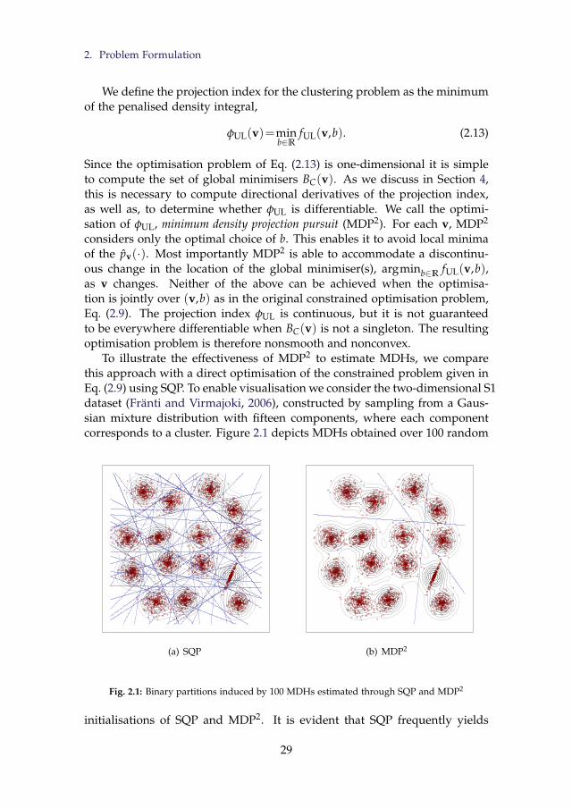
2. Problem Formulation
We define the projection index for the clustering problem as the minimumof the penalised density integral,
φUL(v)=minb∈R
fUL(v,b). (2.13)
Since the optimisation problem of Eq. (2.13) is one-dimensional it is simpleto compute the set of global minimisers BC(v). As we discuss in Section 4,this is necessary to compute directional derivatives of the projection index,as well as, to determine whether φUL is differentiable. We call the optimi-sation of φUL, minimum density projection pursuit (MDP2). For each v, MDP2
considers only the optimal choice of b. This enables it to avoid local minimaof the pv(·). Most importantly MDP2 is able to accommodate a discontinu-ous change in the location of the global minimiser(s), argminb∈R fUL(v,b),as v changes. Neither of the above can be achieved when the optimisa-tion is jointly over (v,b) as in the original constrained optimisation problem,Eq. (2.9). The projection index φUL is continuous, but it is not guaranteedto be everywhere differentiable when BC(v) is not a singleton. The resultingoptimisation problem is therefore nonsmooth and nonconvex.
To illustrate the effectiveness of MDP2 to estimate MDHs, we comparethis approach with a direct optimisation of the constrained problem given inEq. (2.9) using SQP. To enable visualisation we consider the two-dimensional S1dataset (Fränti and Virmajoki, 2006), constructed by sampling from a Gaus-sian mixture distribution with fifteen components, where each componentcorresponds to a cluster. Figure 2.1 depicts MDHs obtained over 100 random
(a) SQP (b) MDP2
Fig. 2.1: Binary partitions induced by 100 MDHs estimated through SQP and MDP2
initialisations of SQP and MDP2. It is evident that SQP frequently yields
29
Chapter 2. Minimum Density Hyperplane: An Unsupervised and Semi-supervisedClassifier
hyperplanes that intersect regions with high probability density thus split-ting clusters. As SQP always converged in these experiments the poor per-formance is solely due to convergence to local minima. In contrast, MDP2
converges to three different solutions over the 100 experiments, all of whichinduce high-quality partitions, and none intersects a high-density cluster.
2.2 Semi-Supervised Classification
In semi-supervised classification labels are available for a subset of the datasample. The resulting classifier needs to predict as accurately as possible thelabelled examples, while avoiding intersection with high-density regions ofthe empirical density. The formulation of the minimum density hyperplaneproblem can readily accommodate partially labelled data by incorporatingthe linear constraints associated with the labelled data into the clustering for-mulation. Without loss of generality assume that the first ` examples arelabelled by y=(y1, . . . ,y`)>∈−1,1`. The MDH for semi-supervised classi-fication is the solution to the problem,
min(v,b)∈bd(Bd)×R
I(v,b), (2.14a)
subject to: yi(v ·xi−b)>0, ∀i=1, . . . ,`, (2.14b)
b−µv+ασv>0, (2.14c)
µv+ασv−b>0, (2.14d)
where I(v,b),µv, and σv are computed over the entire data set. If the la-belled examples are linearly separable by a hyperplane, H(v,b), satisfyingb∈F(v), then the constraints in Eq. (2.14) define a nonempty feasible set ofhyperplanes,
FLB=
H(v,b) |(v,b)∈bd(Bd)×R,b∈F(v),yi(v ·xi−b)>0, ∀i∈1, . . . ,`⊂C.
(2.15)Eqs. (2.14c) and (2.14d) act as a balancing constraint which discourages MDHsthat classify the vast majority of unlabelled data to a single class. Balanc-ing constraints are included in the estimation of S3VMs for the same rea-son (Joachims, 1999; Chapelle and Zien, 2005).
As in the case of clustering, the direct minimisation of Eq. (2.14) frequentlyleads to locally optimal solutions. To mitigate this we again propose a projec-tion pursuit formulation. We define the penalised density integral for semi-supervised classification as,
fSSC(v,b)= fUL(v,b)+γl
∑i=1
max0,−yi(v ·xi−b)1+ε (2.16)
30

3. Connection to Maximum Margin Hyperplanes
where, γ>0 is a user-defined constant, which controls the trade-off betweenreducing the density on the hyperplane, and misclassifying the labelled ex-amples. The projection index is then defined as the minimum of the penaliseddensity integral,
φSSC(v)=minb∈R
fSSC(v,b). (2.17)
Notice also that the projection pursuit formulation benefits from alwayshaving a solution, even in the event that the labelled data are not linearlyseparable.
3 Connection to Maximum Margin Hyperplanes
In this section we discuss the connection between MDHs and maximum(hard) margin hyperplane separators. The margin of a hyperplane H(v,b)with respect to a data set X is defined as the minimum Euclidean distancebetween the hyperplane and its nearest datum,
margin H(v,b)=minx∈X|v ·x−b|. (2.18)
The points whose distance to the hyperplane H(v,b) is equal to the marginof the hyperplane, that is, argminx∈X |v ·x−b|, are called the support pointsof H(v,b). Let F denote the set of feasible hyperplanes; then the maximummargin hyperplane (MMH) H(vm,bm)∈F satisfies,
margin H(vm,bm)= max(v,b)|H(v,b)∈F
margin H(v,b). (2.19)
The main result of this section is Theorem 1, which states that as the band-width parameter, h, is reduced to zero the MDH converges to the maximummargin hyperplane. An intermediate result, Lemma 4, shows that there ex-ists a positive bandwidth, h′>0 such that, for all h∈(0,h′), the partition ofthe data set induced by the MDH is identical to that of maximum marginhyperplane.
To begin with we discuss some assumptions which allow us to presentthe associated theoretical results of this section. As before we assume a fixedand finite data set X ⊂Rd, and approximate its (assumed) underlying proba-bility density function via a kernel density estimator using Gaussian kernelswith isotropic bandwidth matrix h2 I. We assume that the interior of the con-vex hull of the data, Int(convX ), is non-empty, and define C as the set ofhyperplanes that intersect Int(conv X ), as in Eq. (2.5). The set of feasiblehyperplanes, F, for either clustering or the semi-supervised classification sat-isfies F⊂C. By construction every H(v,b)∈F defines a hyperplane whichpartitions X into two non-empty subsets. Observe that if for each v∈bd(Bd)
31
Chapter 2. Minimum Density Hyperplane: An Unsupervised and Semi-supervisedClassifier
the set b∈R|H(v,b)∈F is compact, then by the compactness of bd(Bd) amaximum margin hyperplane in F exists. For both the clustering and semi-supervised classification problems this compactness holds by construction.
Now, for any h>0, let (v?h,b?h)∈bd(Bd)×R parameterise a hyperplane
which achieves the minimal density integral over all hyperplanes in F, forbandwidth matrix h2 I. That is,
I(v?h,b?h)= min
(v,b)|H(v,b)∈FI(v,b|X ,h2 I), (2.20)
where we briefly return to the explicit notation I(v,b|X ,h2 I) to emphasisethe dependence on the bandwidth parameter, h. Following the approachof Tong and Koller (2000) we first show that as the bandwidth, h, is reducedtowards zero, the density on a hyperplane is dominated by its nearest point.This is achieved by establishing that for all sufficiently small values of h, ahyperplane with non-zero margin has lower density integral than any otherhyperplane with smaller margin.
Lemma 3 Take H(v,b)∈F with non-zero margin and 0<δ<margin H(v,b) :=Mv,b. Then ∃h′>0 such that h∈(0,h′) and Mw,c :=margin H(w,c)6Mv,b−δimplies I(v,b)< I(w,c).
Proof Using Eq. (2.3) it is easy to see that,
I(v,b)61
h√
2πexp
−
M2v,b
2h2
,
inf
I(w,c) |Mw,c6Mv,b−δ>
1nh√
2πexp
−(Mv,b−δ)2
2h2
.
Therefore,
06 limh→0+
I(v,b)inf
I(w,c) |Mw,c6Mv,b−δ6 lim
h→0+
nexp−M2
v,b2h2
exp
− (Mv,b−δ)2
2h2
=0.
Therefore, ∃h′>0 such that h∈(0,h′)⇒ I(v,b)
inf
I(w,c)∣∣Mw,c6Mv,b−δ
<1.
An immediate corollary of Lemma 3 is that as h tends to zero the marginof the minimum density hyperplane tends to the maximum margin. How-ever, this does not necessarily ensure the stronger result that the sequenceof minimum density hyperplanes converges to the maximum margin hyper-plane. To establish this we require two technical results, which describe somealgebraic properties of the maximum margin hyperplane, and are provided
32

3. Connection to Maximum Margin Hyperplanes
as part of the proof of Theorem 1 which is given in the appendix to thischapter.
The next lemma uses the previous result to show that there exists a posi-tive bandwidth, h′>0, such that an MDH estimated using h∈(0,h′) inducesthe same partition of X as the MMH. The result assumes that the maximummargin hyperplane is unique. Notice that if X is a sample of realisations ofa continuous random variable then this uniqueness holds with probability 1.
Lemma 4 Suppose there is a unique hyperplane in F with maximum margin, whichcan be parameterised by (vm,bm)∈bd(Bd)×R. Then ∃h′>0 s.t. h∈(0,h′)⇒H(v?
h,b?h) induces the same partition of X as H(vm,bm).
Proof Let M=marginH(vm,bm). Since X is finite ∃δ>0 s.t. any hyper-plane H(w,c)∈F inducing a partition of X different than that induced byH(vm,bm), satisfies margin H(w,c)6M−δ. By Lemma 3, ∃h′>0 s.t.,
h∈(0,h′)⇒H(v?h,b?h)/∈H(w,c) |margin H(w,c)6M−δ ,
which completes the proof.
The next theorem is the main result of this section, and states that the MDHconverges to the MMH as the bandwidth parameter is reduced to zero. No-tice that by the non-unique representation of hyperplanes, the maximummargin hyperplane has two parameterisations in C, namely (vm,bm) and(−vm,−bm). Convergence to the maximum margin hyperplane is thereforeequivalent to showing that,
min‖(v?h,b?h)−(vm,bm)‖,‖(v?
h,b?h)+(vm,bm)‖→0 as h→0+.
Theorem 1 Suppose there is a unique hyperplane in F with maximum margin,which can be parameterised by (vm,bm)∈bd(Bd)×R. Then,
limh→0+
min‖(v?h,b?h)−(vm,bm)‖,‖(v?
h,b?h)+(vm,bm)‖=0.
The set F used in Theorem 1 is generic so it can capture the constraintsassociated with both clustering and semi-supervised classification, Eq. (2.9),and Eq. (2.14) respectively. In the case of semi-supervised classification wemust also assume that the labelled data are linearly separable. Theorem 1 isnot directly applicable to the MDP2 formulations as in this case the functionbeing minimised is not the density on a hyperplane. The next two subsectionsestablish this result for the MDP2 formulation of the unsupervised and semi-supervised problem.
33
Chapter 2. Minimum Density Hyperplane: An Unsupervised and Semi-supervisedClassifier
3.1 MDP2 for Clustering
We have shown that for the constrained optimisation formulation the min-imum density hyperplane converges to the maximum margin hyperplanewithin the feasible set, FCL⊂C. In addition, Proposition 2 places a boundon the difference between the optima for the two problems, in terms of theparameter η. Combining these we can show that the optimal solution to thepenalised MDP2 formulation converges to the maximum margin hyperplanein FCL, provided the parameters within the penalty term suitably depend onthe bandwidth parameter, h. While the general case can be shown, for ease ofexposition we make the simplifying assumption that the maximum marginhyperplane is strictly feasible, i.e., if (vm,bm) parameterises the maximummargin hyperplane then bm∈(µvm−ασvm ,µvm +ασvm).
For h,η, L>0 define (v?h,η,L,b?h,η,L) to be any global minimiser of fCL, i.e.,
fCL(v?h,η,L,b?h,η,L)= min
(v,b)∈bd(Bd)×RfCL(v,b).
Lemma 5 Suppose there is a unique hyperplane in FCL with maximum margin,which can be parameterised by (vm,bm)∈bd(Bd)×R. Suppose further that bm∈(µvm−ασvm ,µvm +ασvm). For h>0, let L(h)=(e1/2h2
√2π)−1, and 0<η(h)6h.
Then,
limh→0+
min‖(v?h,η(h),L(h),b
?h,η(h),L(h))−(vm,bm)‖,
‖(v?h,η(h),L(h),b
?h,η(h),L(h))+(vm,bm)‖=0.
Proof Let M=marginH(vm,bm) and as in the proof of Lemma 4, let δ>0be such that any hyperplane inducing a different partition from H(vm,bm)has margin at most M−δ. Since H(vm,bm) is strictly feasible it must bethe unique maximum margin hyperplane in Fδ
CL :=(v,b)∈bd(Bd)×R|b∈Bδ/2(F(v)), since the margins of the locally maximum margin hyperplanesfor each partition of X can increase by at most δ/2. We have used the notationBδ/2(F(v)) to denote the neighbourhood of F(v) given by r∈R|d(r,F(v))<δ/2. Observe now that for 0<h<δ/2 we have H(v?
h,η(h),L(h),b?h,η(h),L(h))∈
FδCL, by Proposition 2. In addition, by Theorem 1, we know that the minimis-
ers of I(v,b) over FδCL, say H(vδ
h,bδh), satisfy
limh→0+
min‖(vδ
h,bδh)−(vm,bm)‖,‖(vδ
h,bδh)+(vm,bm)‖
=0.
Now, since H(vm,bm) is strictly feasible ∃ε′>0 s.t. (v,b)∈Bε′((vm,bm),−(vm,bm))⇒H(v,b)∈FCL. Then for any 0<ε<ε′ there exists h′>0 s.t. for0<h<h′ both (vδ
h,bδh)∈Bε((vm,bm),−(vm,bm))⇒H(vδ
h,bδh)∈FCL and
H(v?h,η(h),L(h),b
?h,η(h),L(h))∈Fδ
CL. Now for H(v,b)∈FδCL\FCL we know that I(v,b)
34
3. Connection to Maximum Margin Hyperplanes
< fCL(v,b), whereas for H(v,b)∈FCL, I(v,b)= fCL(v,b) and therefore the min-imiser of fCL(v,b) must lie in the neighbourhood Bε((vm,bm),−(vm,bm)),and the result follows.
3.2 MDP2 for Semi-Supervised Classification
Denote the set of hyperplanes which correctly classify the labelled data byFLB. Under the assumption that ∃H(v,b)∈FLB∩FCL with non-zero margin,we can show that, provided the parameter γ does not shrink too quicklywith h, the hyperplane that minimises fSSC converges to the maximum mar-gin hyperplane contained in FLB∩FCL, where as before we assume that sucha maximum margin hyperplane is strictly feasible. To establish this resultit is sufficient to show that there exists h′>0 such that for all h∈(0,h′), theoptimal hyperplane H(v?
h,η,L,γ,b?h,η,L,γ) correctly classifies all the labelled ex-amples. If this holds, then fSSC(v?
h,η,L,γ,b?h,η,L,γ)= fUL(v?h,η,L,γ,b?h,η,L,γ) for all
sufficiently small h, and hence Lemma 5 can be applied to establish the result.The proof relies on the fact that the penalty terms associated with the knownlabels in Eq. (2.16) are polynomials in b. Provided that γ is bounded belowby a polynomial in h, the value of the penalty terms for hyperplanes that donot correctly classify the labelled data dominate the value of the density inte-gral as h approaches zero. Therefore the optimal hyperplane must correctlyclassify the labelled data for small values of h.
Lemma 6 Define FLB=H(v,b)∣∣yi(v ·xi−b)>0,∀i=1, . . . ,` and FCL=H(v,b)
∣∣µv−ασv6b6µv+ασv and assume that FSSC=FLB∩FCL 6=∅ and that ∃H(v,b)∈FSSC with non-zero margin. For h>0, let L(h)=(e1/2h2
√2π)−1, 0<η(h)6h and
γ(h)>hr for some r>0. Then there exists h′>0 s.t. h∈(0,h′)⇒H(
v?h,η(h),L(h),γ(h),
b?h,η(h),L(h),γ(h)
)∈FLB.
Proof Consider H(v,b) 6∈FLB. Then,
fSSC(v,b)>1
n√
2πhexp(−ν2
?/2h2)+γ(h)ν1+ε? >γ(h)ν1+ε
? ,
where ν?>0 minimises 1n√
2πhexp(−ν2/2h2)+γ(h)ν1+ε. Therefore, ν? is the
unique positive number satisfying,
1n√
2πhexp
(− ν2
?
2h2
)(− ν?
h2
)+(1+ε)γ(h)νε
?=0
⇒ν1−ε? =(1+ε)γ(h)n
√2πh3 exp
(ν2?
2h2
)⇒ν?>
((1+ε)γ(h)n
√2πh3
)1/1−ε.
35

Chapter 2. Minimum Density Hyperplane: An Unsupervised and Semi-supervisedClassifier
We therefore have,
fSSC(v,b) > γ(h)((1+ε)γ(h)n
√2πh3
) 1+ε1−ε
= Kγ(h)2
1−ε h3(1+ε)
1−ε
> Kh2r+3(1+ε)
1−ε ,
where K is a constant which can be chosen independent of (v,b). Finally, forany H(v′,b′)∈FSSC with non-zero margin, ∃h′>0 s.t.
h∈(0,h′)⇒ fSSC(v′,b′)= I(v′,b′)<Kh2r+3(1+ε)
1−ε < fSSC(v,b).
Since K is independent of (v,b), the result follows. The final set of inequalitiesholds since the hyperplane H(v′,b′) is assumed to have non-zero margin, sayMv′ ,b′>0, and hence I(v′,b′)6 1
h√
2πexp−Mv′ ,b′/2h2, which tends to zero
faster than any polynomial in h, as h→0+.
4 Estimation of Minimum Hyperplanes
In this section we discuss the computation of minimum density hyperplanes.We first investigate the continuity and differentiability properties required tooptimise the projection indices φUL(v) and φSSC(v).
Since the domain of both projection indices, φUL(v) and φSSC(v), is theboundary of the unit-sphere in Rd it is more convenient to express v in termsof spherical coordinates,
vi(θ)=
cos(θi)∏i−1
j=1 sin(θj), i=1, . . . ,d−1
∏d−1j=1 sin(θj), i=d,
(2.21)
where θ∈Θ=[0,π]d−2× [0,2π] is called the projection angle. Using sphericalcoordinates renders the domain, Θ, convex and compact, and reduces dimen-sionality by one.
As the following discussion applies to both φUL(v) and φSSC(v) we denotea generic projection index φ :Θ→R, and the associated set of minimisers, as,
φ(θ)=minb∈A
f (v(θ),b), (2.22)
B?(θ)=
b∈A∣∣ f (v(θ),b)=φ(θ)
, (2.23)
where f (v(θ),b) is continuously differentiable, A⊂R is compact and convex,and the correspondence B?(θ) gives the set of global minimisers of f (v(θ),b)for each θ. The definition of A is not critical our formulation. Setting,
A⊃[
minv∈bd(Bd)
µv−ασp−η, maxv∈bd(Bd)
µv+ασp+η
], (2.24)
36
4. Estimation of Minimum Hyperplanes
where σ2p is the variance of the projections along the first principal compo-
nent, ensures that the set of hyperplanes that satisfy the constraint of Eq. (2.7)will be a subset of A for all v.
Berge’s maximum theorem (Berge, 1963; Polak, 1987), establishes the con-tinuity of φ(θ) and the upper-semicontinuity (u.s.c.) of the correspondenceB?(θ). Theorem 3.1 in (Polak, 1987) enables us to establish that φ(θ) is locallyLipschitz continuous. Using Theorem 4.13 of Bonnans and Shapiro (2000)we can further show that φ(θ) is directionally differentiable everywhere. Thedirectional derivative at θ in the direction ν is given by,
dφ(θ;ν)= minb∈B?(θ)
Dθ f (v(θ),b) ·ν, (2.25)
where Dθ denotes the derivative with respect to θ. It is clear from Eq. (2.25)that φ(θ) is differentiable if Dθ f (v(θ),b) is the same for all b∈B?(θ). If B(θ)is a singleton then this condition is trivially satisfied and φ(θ) is continuouslydifferentiable at θ.
It is possible to construct examples in which B(θ) is not a singleton. How-ever, with the exception of contrived examples, our experience with real andsimulated datasets indicates that when h is set through standard bandwidthselection rules B(θ) is almost always a singleton over the optimisation path.
Proposition 7 Suppose B(θ) is a singleton for almost all θ∈Θ. Then φ(θ) is con-tinuously differentiable almost everywhere.
Proof The result follows immediately from the fact that if B(θ)=b is asingleton, then the derivative Dφ(θ)=Dθ f (v(θ),b), which is continuous.
Wolfe (1972) has provided early examples of how standard gradient-basedmethods can fail to converge to a local optimum when used to minimise non-smooth functions. In the last decade a new class of nonsmooth optimisationalgorithms has been developed based on gradient sampling (Burke et al.,2006). Gradient sampling methods use generalised gradient descent to findlocal minima. At each iteration points are randomly sampled in a radiusε of the current candidate solution, and the gradient at each point is com-puted. The convex hull of these gradients serves as an approximation of theε-Clarke generalised gradient (Burke et al., 2002). The minimum element inthe convex hull of these gradients is a descent direction. The gradient sam-pling algorithm progressively reduces the sampling radius so that the convexhull approximates the Clarke generalised gradient. When the origin is con-tained in the Clarke generalised gradient there is no direction of descent, andhence the current candidate solution is a local minimum. Gradient samplingachieves almost sure global convergence for functions that are locally Lip-schitz continuous and almost everywhere continuously differentiable. It isalso well documented that it is an effective optimisation method for func-tions that are only locally Lipschitz continuous.
37
Chapter 2. Minimum Density Hyperplane: An Unsupervised and Semi-supervisedClassifier
4.1 Computational Complexity
In this subsection we analyse the computational complexity of MDP2. Ateach iteration the algorithm projects the data sample onto v(θ) which in-volves O(nd) operations. To compute the projection index, φ(θ), we need tominimise the penalised density integral, f (v(θ),b). This can be achieved byfirst evaluating f (v(θ),b) on a grid of m points, to bracket the location of theminimiser, and then applying bisection to compute the minimiser(s) withinthe desired accuracy. The main computational cost of this procedure is due tothe first step which involves m evaluations of a kernel density estimator withn kernels. Using the improved fast Gauss transform (Morariu et al., 2008)this can be performed in O(m+n) operations, instead of O(mn). Bisectionrequires O(− log2 ε) iterations to locate the minimiser with accuracy ε.
If the minimiser of the penalised density integral b?=argminb∈A f (v(θ),b),is unique the projection index is continuously differentiable at θ. To obtainthe derivative of the projection index it is convenient to define the projectionfunction, P(v)=(x1 ·v, . . . ,xn ·v)> . An application of the chain rule yields,
dθφ=Dθ f (v(θ),b?)=DP f (v(θ),b?)DvPDθv (2.26)
where the derivative of the projections of the data sample with respect to vis equal to the data matrix, DvP=(x1, . . . ,xn)>; and Dθv is the derivative ofv with respect to the projection angle, which yields a d×(d−1) matrix. Thecomputation of the derivative therefore requires O(d(n+d)) operations.
The original GS algorithm requires O(d) gradient evaluations at each it-eration which is costly. Curtis and Que (2013) have developed an adaptivegradient sampling algorithm that requires O(1) gradient evaluations in eachiteration. More recently, Lewis and Overton (2013) have strongly advocatedthat for the minimisation of nonsmooth, nonconvex, locally Lipschitz func-tions, a simple BFGS method using inexact line searches is much more effi-cient in practice than gradient sampling, although no convergence guaranteeshave been established for this method. BFGS requires a single gradient eval-uation at each iteration and a matrix vector operation to update the Hessianmatrix approximation. In our experiments we use this algorithm.
5 Experimental Results
In this section we assess the empirical performance of the minimum densityhyperplane approach for clustering and semi-supervised classification. Wecompare performance with existing state-of-the-art methods for both prob-lems on the following 14 benchmark datasets: Banknote authentication (ban-knote), Breast Cancer Winsconsin original (br. cancer), Forest type mapping(forest), Ionosphere, Optical recognition of handwritten digits (optidigits),
38
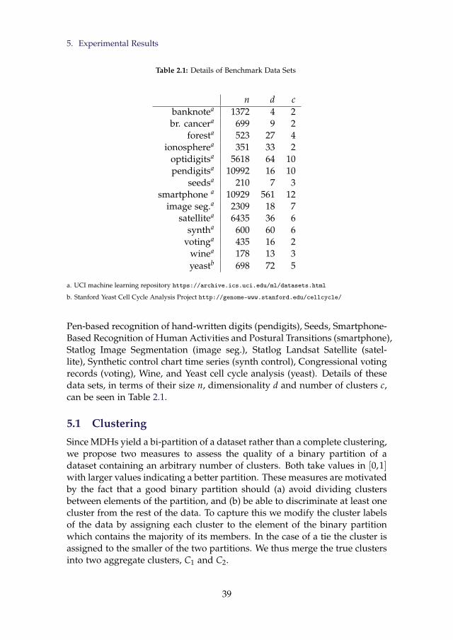
5. Experimental Results
Table 2.1: Details of Benchmark Data Sets
n d cbanknotea 1372 4 2br. cancera 699 9 2
foresta 523 27 4ionospherea 351 33 2
optidigitsa 5618 64 10pendigitsa 10992 16 10
seedsa 210 7 3smartphone a 10929 561 12
image seg.a 2309 18 7satellitea 6435 36 6
syntha 600 60 6votinga 435 16 2
winea 178 13 3yeastb 698 72 5
a. UCI machine learning repository https://archive.ics.uci.edu/ml/datasets.html
b. Stanford Yeast Cell Cycle Analysis Project http://genome-www.stanford.edu/cellcycle/
Pen-based recognition of hand-written digits (pendigits), Seeds, Smartphone-Based Recognition of Human Activities and Postural Transitions (smartphone),Statlog Image Segmentation (image seg.), Statlog Landsat Satellite (satel-lite), Synthetic control chart time series (synth control), Congressional votingrecords (voting), Wine, and Yeast cell cycle analysis (yeast). Details of thesedata sets, in terms of their size n, dimensionality d and number of clusters c,can be seen in Table 2.1.
5.1 Clustering
Since MDHs yield a bi-partition of a dataset rather than a complete clustering,we propose two measures to assess the quality of a binary partition of adataset containing an arbitrary number of clusters. Both take values in [0,1]with larger values indicating a better partition. These measures are motivatedby the fact that a good binary partition should (a) avoid dividing clustersbetween elements of the partition, and (b) be able to discriminate at least onecluster from the rest of the data. To capture this we modify the cluster labelsof the data by assigning each cluster to the element of the binary partitionwhich contains the majority of its members. In the case of a tie the cluster isassigned to the smaller of the two partitions. We thus merge the true clustersinto two aggregate clusters, C1 and C2.
39
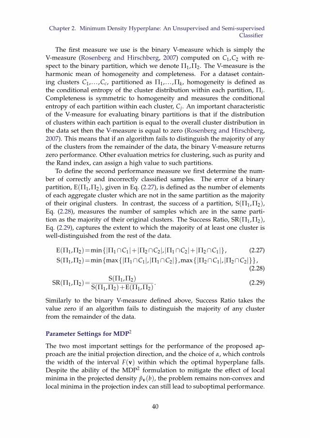
Chapter 2. Minimum Density Hyperplane: An Unsupervised and Semi-supervisedClassifier
The first measure we use is the binary V-measure which is simply theV-measure (Rosenberg and Hirschberg, 2007) computed on C1,C2 with re-spect to the binary partition, which we denote Π1,Π2. The V-measure is theharmonic mean of homogeneity and completeness. For a dataset contain-ing clusters C1, . . . ,Cc, partitioned as Π1, . . . ,Πk, homogeneity is defined asthe conditional entropy of the cluster distribution within each partition, Πi.Completeness is symmetric to homogeneity and measures the conditionalentropy of each partition within each cluster, Cj. An important characteristicof the V-measure for evaluating binary partitions is that if the distributionof clusters within each partition is equal to the overall cluster distribution inthe data set then the V-measure is equal to zero (Rosenberg and Hirschberg,2007). This means that if an algorithm fails to distinguish the majority of anyof the clusters from the remainder of the data, the binary V-measure returnszero performance. Other evaluation metrics for clustering, such as purity andthe Rand index, can assign a high value to such partitions.
To define the second performance measure we first determine the num-ber of correctly and incorrectly classified samples. The error of a binarypartition, E(Π1,Π2), given in Eq. (2.27), is defined as the number of elementsof each aggregate cluster which are not in the same partition as the majorityof their original clusters. In contrast, the success of a partition, S(Π1,Π2),Eq. (2.28), measures the number of samples which are in the same parti-tion as the majority of their original clusters. The Success Ratio, SR(Π1,Π2),Eq. (2.29), captures the extent to which the majority of at least one cluster iswell-distinguished from the rest of the data.
E(Π1,Π2)=min|Π1∩C1|+ |Π2∩C2|, |Π1∩C2|+ |Π2∩C1| , (2.27)
S(Π1,Π2)=minmax|Π1∩C1|, |Π1∩C2| ,max|Π2∩C1|, |Π2∩C2| ,(2.28)
SR(Π1,Π2)=S(Π1,Π2)
S(Π1,Π2)+E(Π1,Π2). (2.29)
Similarly to the binary V-measure defined above, Success Ratio takes thevalue zero if an algorithm fails to distinguish the majority of any clusterfrom the remainder of the data.
Parameter Settings for MDP2
The two most important settings for the performance of the proposed ap-proach are the initial projection direction, and the choice of α, which controlsthe width of the interval F(v) within which the optimal hyperplane falls.Despite the ability of the MDP2 formulation to mitigate the effect of localminima in the projected density pv(b), the problem remains non-convex andlocal minima in the projection index can still lead to suboptimal performance.
40
5. Experimental Results
We have found that this effect is amplified in general when either or both thenumber of dimensions, and the number of high density clusters in the datasetis large. To better handle the effect of local optima, we use multiple initialisa-tions and select the MDH that maximises the relative depth criterion, definedin Eq. (2.30). The relative depth of an MDH, H(v,b), is defined as the smallerof the relative differences in the density on the MDH and its two adjacentmodes in the projected density, pv(·),
RelativeDepth(v,b)=min
pv(ml)− pv(b)pv(b)
,pv(mr)− pv(b)
pv(b)
, (2.30)
where ml and mr are the two adjacent modes in pv(·). If an MDH does notseparate the modes of the projected density, pv(·), then its relative depth isset to zero, signalling a failure of MDP2 to identify a meaningful bi-partition.The relative depth is appealing because it captures the fact that a high qualityseparating hyperplane should have a low density integral, and separate wellthe modes of the projected density pv(·). Note also that the relative depthis equivalent to the inverse of a measure used to define cluster overlap inthe context of Gaussian mixtures (Aitnouri et al., 2000). In all the reportedexperiments we initialise MDP2 to the first and second principal componentand select the MDH with the largest relative depth. For the data sets listedabove it was never the case that both initialisations led to MDHs with zerorelative depth.
The choice of α determines the trade-off between a balanced bi-partitionand the ability to discover lower density hyperplanes. The difficulties asso-ciated with choosing this parameter are illustrated in Figure 2.2. In eachsub-figure the horizontal axis is the candidate projection vector, v, whilethe right vertical axis is the direction of maximum variability orthogonalto v. Points correspond to projections of the data sample onto this two-dimensional space, while colour indicates cluster membership. The solid linedepicts the projected density on v, pv(·), while the dotted line depicts thepenalised function, fUL(v, ·). The scale of both functions is depicted in theleft vertical axis. The solid vertical line indicates the MDH along v. Settingα to a large value can cause MDP2 to focus on hyperplanes that have lowdensity because they partition only a small subset of the dataset as shownin Figure 2.2(a). In contrast smaller values of α may cause the algorithm todisregard valid lower density hyperplane separators (see Figure 2.2(b)), orfor the separating hyperplane to not be a local minimiser of the projecteddensity (see Figure 2.2(c)).
Rather than selecting a single value for α we recommend solving MDP2
repeatedly for an increasing sequence of values in the range αmin,αmax,where each implementation beyond the first is initialised using the solutionto the previous. Setting αmin close to zero forces MDP2 to seek low densityhyperplanes that induce a balanced data partition. This tends to find projec-
41
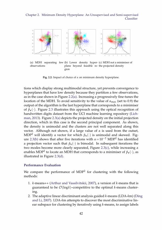
Chapter 2. Minimum Density Hyperplane: An Unsupervised and Semi-supervisedClassifier
−5 0 5
0.0
0.1
0.2
0.3
0.4
0.5
0.6
0.7
(a) MDH separating fewobservations
−5 0 5
0.0
0.1
0.2
0.3
0.4
(b) Lower density hyper-plane beyond feasible re-gion
−4 −2 0 2 4 6 8
0.0
0.1
0.2
0.3
0.4
(c) MDH not a minimiser ofthe projected density
Fig. 2.2: Impact of choice of α on minimum density hyperplane.
tions which display strong multimodal structure, yet prevents convergence tohyperplanes that have low density because they partition a few observations,as in the case shown in Figure 2.2(a). Increasing α progressively fine-tunes thelocation of the MDH. To avoid sensitivity to the value of αmax (set to 0.9) theoutput of the algorithm is the last hyperplane that corresponds to a minimiserof pv(·). Figure 2.3 illustrates this approach using the optical recognition ofhandwritten digits dataset from the UCI machine learning repository (Lich-man, 2013). Figure 2.3(a) depicts the projected density on the initial projectiondirection, which in this case is the second principal component. As shown,the density is unimodal and the clusters are not well separated along thisvector. Although not shown, if a large value of α is used from the outset,MDP2 will identify a vector for which pv(·) is unimodal and skewed. Fig-ure 2.3(b) shows that after five iterations with α=10−2 MDP2 has identifieda projection vector such that pv(·) is bimodal. In subsequent iterations thetwo modes become more clearly separated, Figure 2.3(c), while increasing αenables MDP2 to locate an MDH that corresponds to a minimiser of pv(·), asillustrated in Figure 2.3(d).
Performance Evaluation
We compare the performance of MDP2 for clustering with the followingmethods:
1. k-means++ (Arthur and Vassilvitskii, 2007), a version of k-means that isguaranteed to be O(logk)–competitive to the optimal k-means cluster-ing.
2. The adaptive linear discriminant analysis guided k-means (LDA-km) (Dingand Li, 2007). LDA-km attempts to discover the most discriminative lin-ear subspace for clustering by iteratively using k-means, to assign labels
42
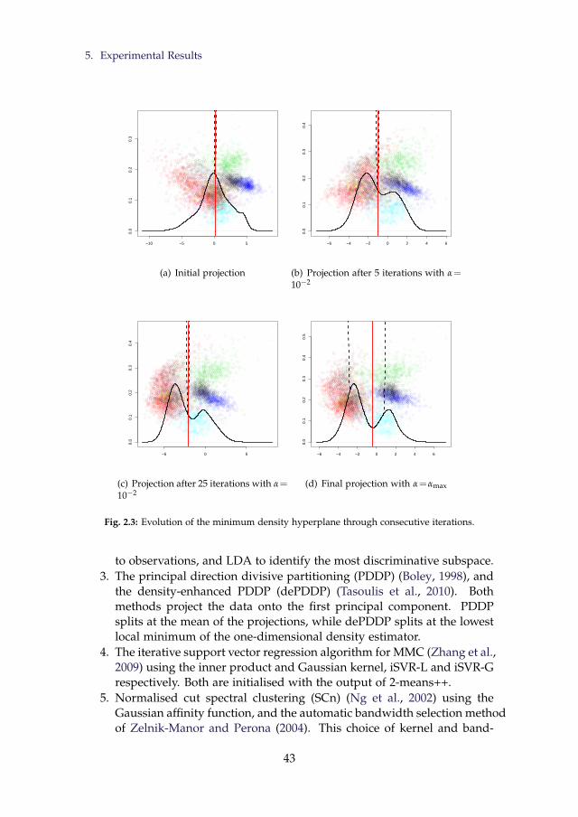
5. Experimental Results
−10 −5 0 5
0.0
0.1
0.2
0.3
(a) Initial projection
−6 −4 −2 0 2 4 6
0.0
0.1
0.2
0.3
0.4
(b) Projection after 5 iterations with α=10−2
−5 0 5
0.0
0.1
0.2
0.3
0.4
(c) Projection after 25 iterations with α=10−2
−6 −4 −2 0 2 4 6
0.0
0.1
0.2
0.3
0.4
0.5
(d) Final projection with α=αmax
Fig. 2.3: Evolution of the minimum density hyperplane through consecutive iterations.
to observations, and LDA to identify the most discriminative subspace.3. The principal direction divisive partitioning (PDDP) (Boley, 1998), and
the density-enhanced PDDP (dePDDP) (Tasoulis et al., 2010). Bothmethods project the data onto the first principal component. PDDPsplits at the mean of the projections, while dePDDP splits at the lowestlocal minimum of the one-dimensional density estimator.
4. The iterative support vector regression algorithm for MMC (Zhang et al.,2009) using the inner product and Gaussian kernel, iSVR-L and iSVR-Grespectively. Both are initialised with the output of 2-means++.
5. Normalised cut spectral clustering (SCn) (Ng et al., 2002) using theGaussian affinity function, and the automatic bandwidth selection methodof Zelnik-Manor and Perona (2004). This choice of kernel and band-
43
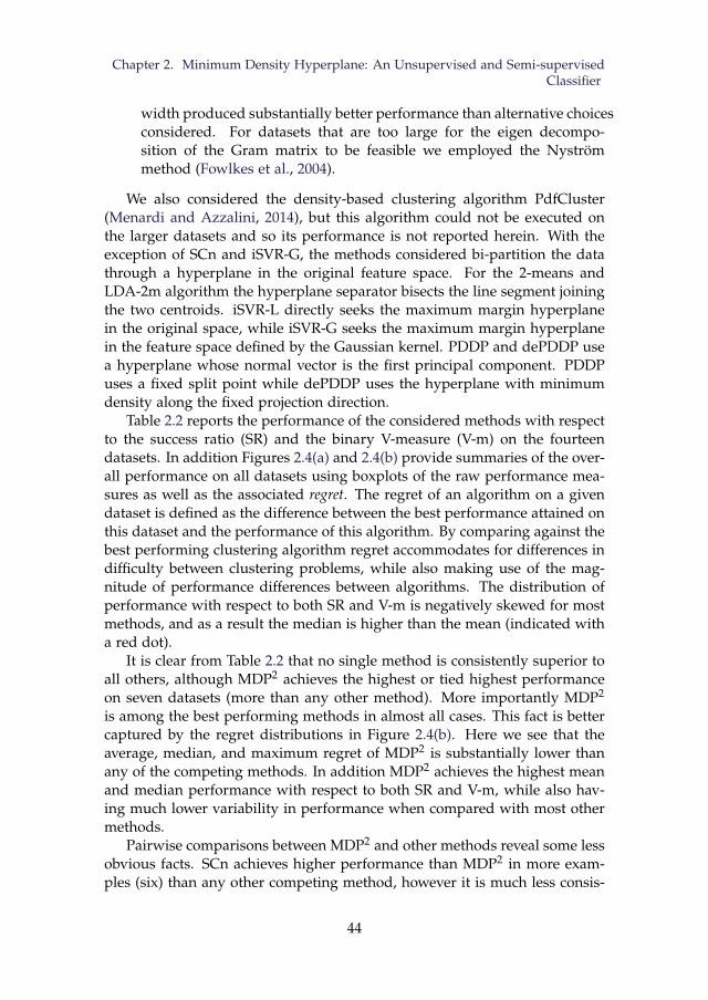
Chapter 2. Minimum Density Hyperplane: An Unsupervised and Semi-supervisedClassifier
width produced substantially better performance than alternative choicesconsidered. For datasets that are too large for the eigen decompo-sition of the Gram matrix to be feasible we employed the Nyströmmethod (Fowlkes et al., 2004).
We also considered the density-based clustering algorithm PdfCluster(Menardi and Azzalini, 2014), but this algorithm could not be executed onthe larger datasets and so its performance is not reported herein. With theexception of SCn and iSVR-G, the methods considered bi-partition the datathrough a hyperplane in the original feature space. For the 2-means andLDA-2m algorithm the hyperplane separator bisects the line segment joiningthe two centroids. iSVR-L directly seeks the maximum margin hyperplanein the original space, while iSVR-G seeks the maximum margin hyperplanein the feature space defined by the Gaussian kernel. PDDP and dePDDP usea hyperplane whose normal vector is the first principal component. PDDPuses a fixed split point while dePDDP uses the hyperplane with minimumdensity along the fixed projection direction.
Table 2.2 reports the performance of the considered methods with respectto the success ratio (SR) and the binary V-measure (V-m) on the fourteendatasets. In addition Figures 2.4(a) and 2.4(b) provide summaries of the over-all performance on all datasets using boxplots of the raw performance mea-sures as well as the associated regret. The regret of an algorithm on a givendataset is defined as the difference between the best performance attained onthis dataset and the performance of this algorithm. By comparing against thebest performing clustering algorithm regret accommodates for differences indifficulty between clustering problems, while also making use of the mag-nitude of performance differences between algorithms. The distribution ofperformance with respect to both SR and V-m is negatively skewed for mostmethods, and as a result the median is higher than the mean (indicated witha red dot).
It is clear from Table 2.2 that no single method is consistently superior toall others, although MDP2 achieves the highest or tied highest performanceon seven datasets (more than any other method). More importantly MDP2
is among the best performing methods in almost all cases. This fact is bettercaptured by the regret distributions in Figure 2.4(b). Here we see that theaverage, median, and maximum regret of MDP2 is substantially lower thanany of the competing methods. In addition MDP2 achieves the highest meanand median performance with respect to both SR and V-m, while also hav-ing much lower variability in performance when compared with most othermethods.
Pairwise comparisons between MDP2 and other methods reveal some lessobvious facts. SCn achieves higher performance than MDP2 in more exam-ples (six) than any other competing method, however it is much less consis-
44
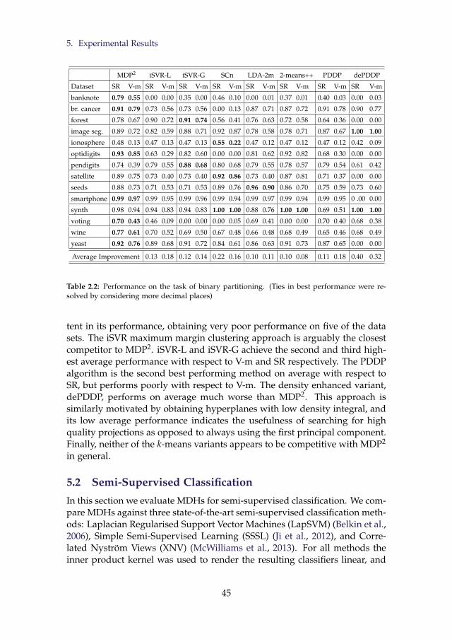
5. Experimental Results
MDP2 iSVR-L iSVR-G SCn LDA-2m 2-means++ PDDP dePDDP
Dataset SR V-m SR V-m SR V-m SR V-m SR V-m SR V-m SR V-m SR V-m
banknote 0.79 0.55 0.00 0.00 0.35 0.00 0.46 0.10 0.00 0.01 0.37 0.01 0.40 0.03 0.00 0.03
br. cancer 0.91 0.79 0.73 0.56 0.73 0.56 0.00 0.13 0.87 0.71 0.87 0.72 0.91 0.78 0.90 0.77
forest 0.78 0.67 0.90 0.72 0.91 0.74 0.56 0.41 0.76 0.63 0.72 0.58 0.64 0.36 0.00 0.00
image seg. 0.89 0.72 0.82 0.59 0.88 0.71 0.92 0.87 0.78 0.58 0.78 0.71 0.87 0.67 1.00 1.00
ionosphere 0.48 0.13 0.47 0.13 0.47 0.13 0.55 0.22 0.47 0.12 0.47 0.12 0.47 0.12 0.42 0.09
optidigits 0.93 0.85 0.63 0.29 0.82 0.60 0.00 0.00 0.81 0.62 0.92 0.82 0.68 0.30 0.00 0.00
pendigits 0.74 0.39 0.79 0.55 0.88 0.68 0.80 0.68 0.79 0.55 0.78 0.57 0.79 0.54 0.61 0.42
satellite 0.89 0.75 0.73 0.40 0.73 0.40 0.92 0.86 0.73 0.40 0.87 0.81 0.71 0.37 0.00 0.00
seeds 0.88 0.73 0.71 0.53 0.71 0.53 0.89 0.76 0.96 0.90 0.86 0.70 0.75 0.59 0.73 0.60
smartphone 0.99 0.97 0.99 0.95 0.99 0.96 0.99 0.94 0.99 0.97 0.99 0.94 0.99 0.95 0 .00 0.00
synth 0.98 0.94 0.94 0.83 0.94 0.83 1.00 1.00 0.88 0.76 1.00 1.00 0.69 0.51 1.00 1.00
voting 0.70 0.43 0.46 0.09 0.00 0.00 0.00 0.05 0.69 0.41 0.00 0.00 0.70 0.40 0.68 0.38
wine 0.77 0.61 0.70 0.52 0.69 0.50 0.67 0.48 0.66 0.48 0.68 0.49 0.65 0.46 0.68 0.49
yeast 0.92 0.76 0.89 0.68 0.91 0.72 0.84 0.61 0.86 0.63 0.91 0.73 0.87 0.65 0.00 0.00
Average Improvement 0.13 0.18 0.12 0.14 0.22 0.16 0.10 0.11 0.10 0.08 0.11 0.18 0.40 0.32
Table 2.2: Performance on the task of binary partitioning. (Ties in best performance were re-solved by considering more decimal places)
tent in its performance, obtaining very poor performance on five of the datasets. The iSVR maximum margin clustering approach is arguably the closestcompetitor to MDP2. iSVR-L and iSVR-G achieve the second and third high-est average performance with respect to V-m and SR respectively. The PDDPalgorithm is the second best performing method on average with respect toSR, but performs poorly with respect to V-m. The density enhanced variant,dePDDP, performs on average much worse than MDP2. This approach issimilarly motivated by obtaining hyperplanes with low density integral, andits low average performance indicates the usefulness of searching for highquality projections as opposed to always using the first principal component.Finally, neither of the k-means variants appears to be competitive with MDP2
in general.
5.2 Semi-Supervised Classification
In this section we evaluate MDHs for semi-supervised classification. We com-pare MDHs against three state-of-the-art semi-supervised classification meth-ods: Laplacian Regularised Support Vector Machines (LapSVM) (Belkin et al.,2006), Simple Semi-Supervised Learning (SSSL) (Ji et al., 2012), and Corre-lated Nyström Views (XNV) (McWilliams et al., 2013). For all methods theinner product kernel was used to render the resulting classifiers linear, and
45
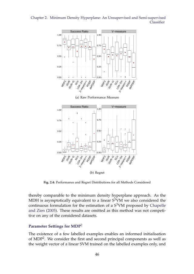
Chapter 2. Minimum Density Hyperplane: An Unsupervised and Semi-supervisedClassifier
Success Ratio V−measure
0.00
0.25
0.50
0.75
1.00
0.00
0.25
0.50
0.75
1.00
MD
P2iS
VRiS
VR−G SC
nLD
A−2m
2−m
eans
++PD
DP
dePD
DP
MD
P2iS
VRiS
VR−G SC
nLD
A−2m
2−m
eans
++PD
DP
dePD
DP
(a) Raw Performance Measure
Success Ratio V−measure
0.00
0.25
0.50
0.75
1.00
0.00
0.25
0.50
0.75
1.00
MD
P2iS
VRiS
VR−G SC
nLD
A−2m
2−m
eans
++PD
DP
dePD
DP
MD
P2iS
VRiS
VR−G SC
nLD
A−2m
2−m
eans
++PD
DP
dePD
DP
(b) Regret
Fig. 2.4: Performance and Regret Distributions for all Methods Considered
thereby comparable to the minimum density hyperplane approach. As theMDH is asymptotically equivalent to a linear S3VM we also considered thecontinuous formulation for the estimation of a S3VM proposed by Chapelleand Zien (2005). These results are omitted as this method was not competi-tive on any of the considered datasets.
Parameter Settings for MDP2
The existence of a few labelled examples enables an informed initialisationof MDP2. We consider the first and second principal components as well asthe weight vector of a linear SVM trained on the labelled examples only, and
46
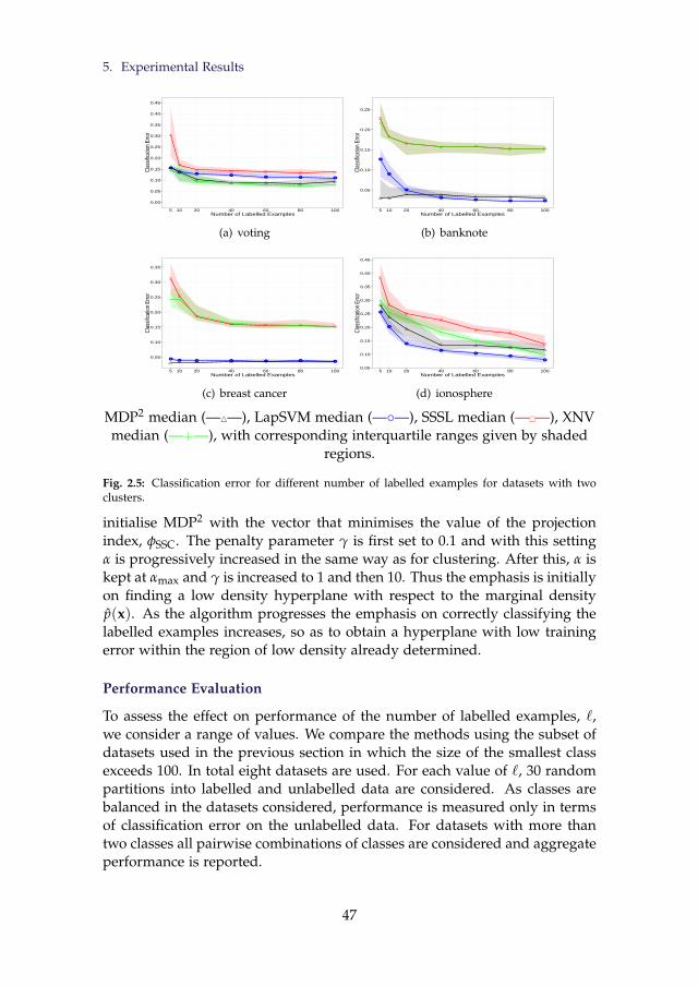
5. Experimental Results
0.00
0.05
0.10
0.15
0.20
0.25
0.30
0.35
0.40
0.45
5 10 20 40 60 80 100Number of Labelled Examples
Clas
sifica
tion
Erro
r
(a) voting
0.05
0.10
0.15
0.20
0.25
5 10 20 40 60 80 100Number of Labelled Examples
Clas
sifica
tion
Erro
r
(b) banknote
0.05
0.10
0.15
0.20
0.25
0.30
0.35
5 10 20 40 60 80 100Number of Labelled Examples
Clas
sifica
tion
Erro
r
(c) breast cancer
0.05
0.10
0.15
0.20
0.25
0.30
0.35
0.40
0.45
5 10 20 40 60 80 100Number of Labelled Examples
Clas
sifica
tion
Erro
r
(d) ionosphere
MDP2 median (—4—), LapSVM median (——), SSSL median (——), XNVmedian (—+—), with corresponding interquartile ranges given by shaded
regions.
Fig. 2.5: Classification error for different number of labelled examples for datasets with twoclusters.
initialise MDP2 with the vector that minimises the value of the projectionindex, φSSC. The penalty parameter γ is first set to 0.1 and with this settingα is progressively increased in the same way as for clustering. After this, α iskept at αmax and γ is increased to 1 and then 10. Thus the emphasis is initiallyon finding a low density hyperplane with respect to the marginal densityp(x). As the algorithm progresses the emphasis on correctly classifying thelabelled examples increases, so as to obtain a hyperplane with low trainingerror within the region of low density already determined.
Performance Evaluation
To assess the effect on performance of the number of labelled examples, `,we consider a range of values. We compare the methods using the subset ofdatasets used in the previous section in which the size of the smallest classexceeds 100. In total eight datasets are used. For each value of `, 30 randompartitions into labelled and unlabelled data are considered. As classes arebalanced in the datasets considered, performance is measured only in termsof classification error on the unlabelled data. For datasets with more thantwo classes all pairwise combinations of classes are considered and aggregateperformance is reported.
47
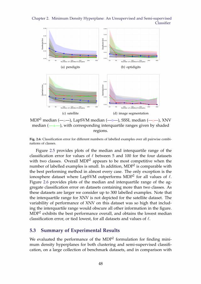
Chapter 2. Minimum Density Hyperplane: An Unsupervised and Semi-supervisedClassifier
0.00
0.02
0.04
0.06
0.08
10 50 100 150 200 250 300Number of Labelled Examples
Clas
sifica
tion
Erro
r
(a) pendigits
0.00
0.01
0.02
0.03
0.04
0.05
10 50 100 150 200 250 300Number of Labelled Examples
Clas
sifica
tion
Erro
r
(b) optidigits
0.05
0.10
10 50 100 150 200 250 300Number of Labelled Examples
Clas
sifica
tion
Erro
r
(c) satellite
0.00
0.02
0.04
0.06
10 50 100 150 200 250 300Number of Labelled Examples
Clas
sifica
tion
Erro
r
(d) image segmentation
MDP2 median (—4—), LapSVM median (——), SSSL median (——), XNVmedian (—+—), with corresponding interquartile ranges given by shaded
regions.
Fig. 2.6: Classification error for different numbers of labelled examples over all pairwise combi-nations of classes.
Figure 2.5 provides plots of the median and interquartile range of theclassification error for values of ` between 5 and 100 for the four datasetswith two classes. Overall MDP2 appears to be most competitive when thenumber of labelled examples is small. In addition, MDP2 is comparable withthe best performing method in almost every case. The only exception is theionosphere dataset where LapSVM outperforms MDP2 for all values of `.Figure 2.6 provides plots of the median and interquartile range of the ag-gregate classification error on datasets containing more than two classes. Asthese datasets are larger we consider up to 300 labelled examples. Note thatthe interquartile range for XNV is not depicted for the satellite dataset. Thevariability of performance of XNV on this dataset was so high that includ-ing the interquartile range would obscure all other information in the figure.MDP2 exhibits the best performance overall, and obtains the lowest medianclassification error, or tied lowest, for all datasets and values of `.
5.3 Summary of Experimental Results
We evaluated the performance of the MDP2 formulation for finding mini-mum density hyperplanes for both clustering and semi-supervised classifi-cation, on a large collection of benchmark datasets, and in comparison with
48
6. Conclusions
state-of-the-art methods for both problems.For clustering, we found that no single method was consistently superior
to all others. This is a result of the vastly differing nature of the datasetsin terms of size, dimensionality, number and shape of clusters, etc. MDP2
achieved the best performance on more datasets than any of the competingmethods, and importantly was competitive with the best performing methodin almost every dataset considered. All other methods performed poorlyin at least as many examples. Boxplots of both the raw performance andperformance regret, which measures the difference between each method andthe best performing method on each dataset, allowed us to summarise thecomparative performance of the different methods across datasets. The meanand median raw performance of MDP2 is substantially higher than the nextbest performing method, and the regret is also substantially lower.
In the case of semi-supervised classification it was apparent that MDP2 isextremely competitive when the number of labelled examples is (very) small,but that in some cases its performance does not improve as much as thatof the other methods considered, when the labelled examples become moreabundant. Our experiments suggest that overall MDP2 is very competitivewith the state-of-the-art for semi-supervised classification problems.
6 Conclusions
We proposed a new hyperplane classifier for clustering and semi-supervisedclassification. The proposed approach is motivated by determining low den-sity linear separators of the high-density clusters within a dataset. This isachieved by minimising the integral of the empirical density along the hy-perplane, which is computed through kernel density estimation. To the bestof our knowledge this is the first direct implementation of the low densityseparation assumption that underlies high-density clustering and numerousinfluential semi-supervised classification methods. We show that the min-imum density hyperplane classifier is asymptotically connected with max-imum margin support vector classifiers, thereby establishing an importantlink between the proposed approach, maximum margin clustering, and semi-supervised support vector machines.
The proposed formulation allows us to evaluate the integral of the densityon a hyperplane by projecting the data onto the vector normal to the hyper-plane, and estimating a univariate kernel density estimator. This enables usto apply our method effectively and efficiently on datasets of much higherdimensionality than is generally possible for density based clustering meth-ods. To mitigate the problem of convergence to locally optimal solutions weproposed a projection pursuit formulation.
We evaluated the minimum density hyperplane approach on a large col-
49
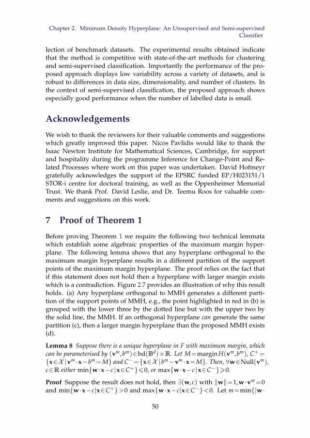
Chapter 2. Minimum Density Hyperplane: An Unsupervised and Semi-supervisedClassifier
lection of benchmark datasets. The experimental results obtained indicatethat the method is competitive with state-of-the-art methods for clusteringand semi-supervised classification. Importantly the performance of the pro-posed approach displays low variability across a variety of datasets, and isrobust to differences in data size, dimensionality, and number of clusters. Inthe context of semi-supervised classification, the proposed approach showsespecially good performance when the number of labelled data is small.
Acknowledgements
We wish to thank the reviewers for their valuable comments and suggestionswhich greatly improved this paper. Nicos Pavlidis would like to thank theIsaac Newton Institute for Mathematical Sciences, Cambridge, for supportand hospitality during the programme Inference for Change-Point and Re-lated Processes where work on this paper was undertaken. David Hofmeyrgratefully acknowledges the support of the EPSRC funded EP/H023151/1STOR-i centre for doctoral training, as well as the Oppenheimer MemorialTrust. We thank Prof. David Leslie, and Dr. Teemu Roos for valuable com-ments and suggestions on this work.
7 Proof of Theorem 1
Before proving Theorem 1 we require the following two technical lemmatawhich establish some algebraic properties of the maximum margin hyper-plane. The following lemma shows that any hyperplane orthogonal to themaximum margin hyperplane results in a different partition of the supportpoints of the maximum margin hyperplane. The proof relies on the fact thatif this statement does not hold then a hyperplane with larger margin existswhich is a contradiction. Figure 2.7 provides an illustration of why this resultholds. (a) Any hyperplane orthogonal to MMH generates a different parti-tion of the support points of MMH, e.g., the point highlighted in red in (b) isgrouped with the lower three by the dotted line but with the upper two bythe solid line, the MMH. If an orthogonal hyperplane can generate the samepartition (c), then a larger margin hyperplane than the proposed MMH exists(d).
Lemma 8 Suppose there is a unique hyperplane in F with maximum margin, whichcan be parameterised by (vm,bm)∈bd(Bd)×R. Let M=margin H(vm,bm), C+=x∈X |vm ·x−bm=M and C−=x∈X |bm−vm ·x=M. Then, ∀w∈Null(vm),c∈R either minw ·x−c |x∈C+60, or maxw ·x−c |x∈C−>0.
Proof Suppose the result does not hold, then ∃(w,c) with ‖w‖=1,w ·vm=0and minw ·x−c|x∈C+>0 and maxw ·x−c|x∈C−<0. Let m=min|w ·
50
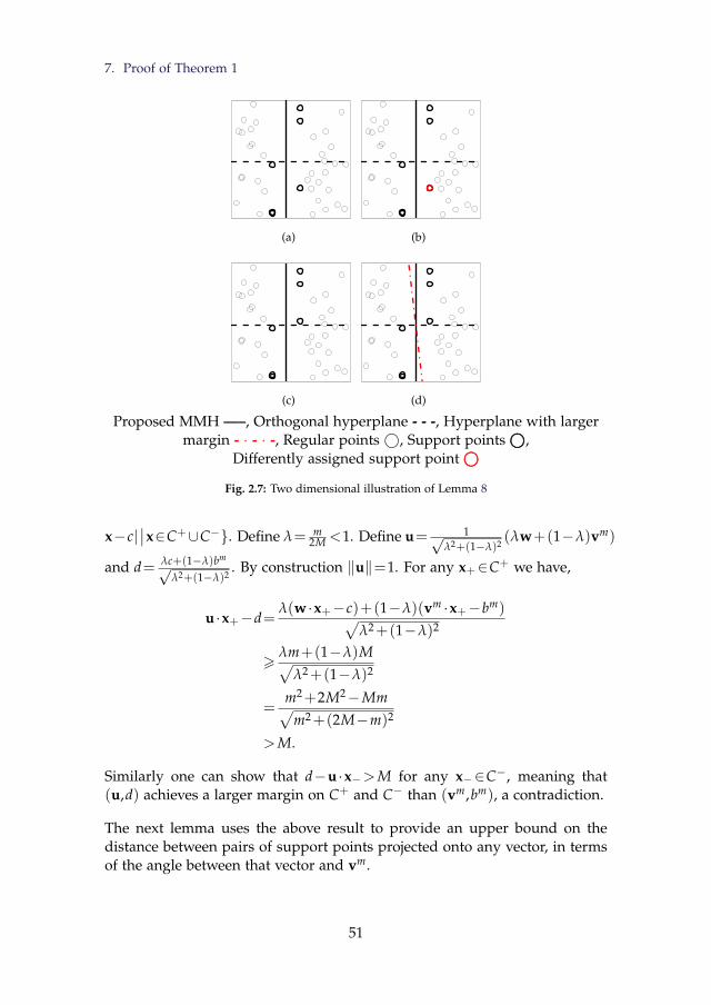
7. Proof of Theorem 1
(a) (b)
(c) (d)
Proposed MMH —–, Orthogonal hyperplane - - -, Hyperplane with largermargin - · - · -, Regular points©, Support points©©©,
Differently assigned support point©©©
Fig. 2.7: Two dimensional illustration of Lemma 8
x−c|∣∣x∈C+∪C−. Define λ= m
2M <1. Define u= 1√λ2+(1−λ)2
(λw+(1−λ)vm)
and d= λc+(1−λ)bm√λ2+(1−λ)2
. By construction ‖u‖=1. For any x+∈C+ we have,
u ·x+−d=λ(w ·x+−c)+(1−λ)(vm ·x+−bm)√
λ2+(1−λ)2
>λm+(1−λ)M√
λ2+(1−λ)2
=m2+2M2−Mm√
m2+(2M−m)2
>M.
Similarly one can show that d−u ·x−>M for any x−∈C−, meaning that(u,d) achieves a larger margin on C+ and C− than (vm,bm), a contradiction.
The next lemma uses the above result to provide an upper bound on thedistance between pairs of support points projected onto any vector, in termsof the angle between that vector and vm.
51
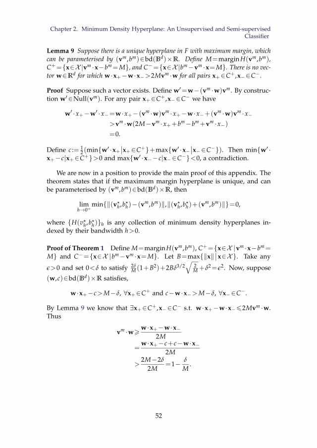
Chapter 2. Minimum Density Hyperplane: An Unsupervised and Semi-supervisedClassifier
Lemma 9 Suppose there is a unique hyperplane in F with maximum margin, whichcan be parameterised by (vm,bm)∈bd(Bd)×R. Define M=margin H(vm,bm),C+=x∈X |vm ·x−bm=M, and C−=x∈X |bm−vm ·x=M. There is no vec-tor w∈Rd for which w ·x+−w ·x−>2Mvm ·w for all pairs x+∈C+,x−∈C−.
Proof Suppose such a vector exists. Define w′=w−(vm ·w)vm. By construc-tion w′∈Null(vm). For any pair x+∈C+,x−∈C− we have
w′ ·x+−w′ ·x−=w ·x+−(vm ·w)vm ·x+−w ·x−+(vm ·w)vm ·x−>vm ·w(2M−vm ·x++bm−bm+vm ·x−)=0.
Define c := 12 (minw′ ·x+
∣∣x+∈C++maxw′ ·x−∣∣x−∈C−). Then minw′ ·
x+−c|x+∈C+>0 and maxw′ ·x−−c|x−∈C−<0, a contradiction.
We are now in a position to provide the main proof of this appendix. Thetheorem states that if the maximum margin hyperplane is unique, and canbe parameterised by (vm,bm)∈bd(Bd)×R, then
limh→0+
min‖(v?h,b?h)−(vm,bm)‖,‖(v?
h,b?h)+(vm,bm)‖=0,
where H(v?h,b?h)h is any collection of minimum density hyperplanes in-dexed by their bandwidth h>0.
Proof of Theorem 1 Define M=margin H(vm,bm), C+=x∈X |vm ·x−bm=M and C−=x∈X |bm−vm ·x=M. Let B=max‖x‖
∣∣x∈X. Take any
ε>0 and set 0<δ to satisfy 2δM (1+B2)+2Bδ3/2
√2M +δ2=ε2. Now, suppose
(w,c)∈bd(Bd)×R satisfies,
w ·x+−c>M−δ, ∀x+∈C+ and c−w ·x−>M−δ, ∀x−∈C−.
By Lemma 9 we know that ∃x+∈C+,x−∈C− s.t. w ·x+−w ·x−62Mvm ·w.Thus
vm ·w>w ·x+−w ·x−2M
=w ·x+−c+c−w ·x−
2M
>2M−2δ
2M=1− δ
M.
52
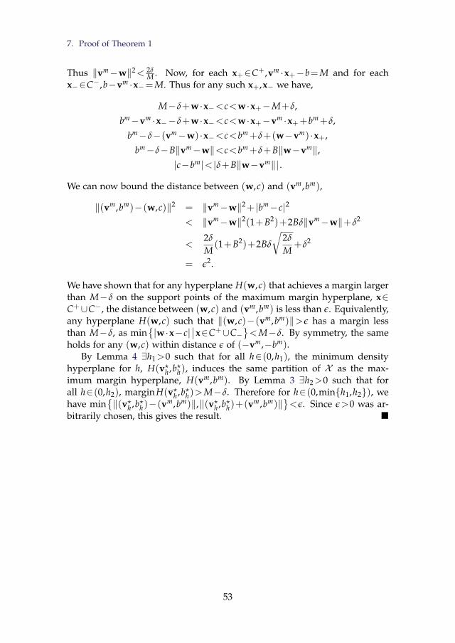
7. Proof of Theorem 1
Thus ‖vm−w‖2< 2δM . Now, for each x+∈C+,vm ·x+−b=M and for each
x−∈C−,b−vm ·x−=M. Thus for any such x+,x− we have,
M−δ+w ·x−<c<w ·x+−M+δ,
bm−vm ·x−−δ+w ·x−<c<w ·x+−vm ·x++bm+δ,
bm−δ−(vm−w) ·x−<c<bm+δ+(w−vm) ·x+,
bm−δ−B‖vm−w‖<c<bm+δ+B‖w−vm‖,|c−bm|< |δ+B‖w−vm‖| .
We can now bound the distance between (w,c) and (vm,bm),
‖(vm,bm)−(w,c)‖2 = ‖vm−w‖2+ |bm−c|2
< ‖vm−w‖2(1+B2)+2Bδ‖vm−w‖+δ2
<2δ
M(1+B2)+2Bδ
√2δ
M+δ2
= ε2.
We have shown that for any hyperplane H(w,c) that achieves a margin largerthan M−δ on the support points of the maximum margin hyperplane, x∈C+∪C−, the distance between (w,c) and (vm,bm) is less than ε. Equivalently,any hyperplane H(w,c) such that ‖(w,c)−(vm,bm)‖>ε has a margin lessthan M−δ, as min
|w ·x−c|
∣∣x∈C+∪C−<M−δ. By symmetry, the same
holds for any (w,c) within distance ε of (−vm,−bm).By Lemma 4 ∃h1>0 such that for all h∈(0,h1), the minimum density
hyperplane for h, H(v?h,b?h), induces the same partition of X as the max-
imum margin hyperplane, H(vm,bm). By Lemma 3 ∃h2>0 such that forall h∈(0,h2), margin H(v?
h,b?h)>M−δ. Therefore for h∈(0,minh1,h2), wehave min
‖(v?
h,b?h)−(vm,bm)‖,‖(v?h,b?h)+(vm,bm)‖
<ε. Since ε>0 was ar-
bitrarily chosen, this gives the result.
53

Chapter 3
Projection Pursuit Based onSpectral Connectivity
This chapter contains two parts. The first part provides a rigorous investi-gation into projection pursuit based on spectral connectivity for the purposeof unsupervised data partitioning. The spectral connectivity of a data setrefers to the optimal value of a relaxation of the normalised graph cut, interms of a graph defined over the data set in which edges correspond tothe similarities between data. A projection along which a data set has lowspectral connectivity in general corresponds to a projection along which thedata display multiple, well separated clusters. In this context a cluster is asubgraph containing relatively high edge weights, and hence mostly similardata points.
The second part extends the methodology developed in the first part tothe problem of semi-supervised classification. The graph formulation pro-vides a useful framework for incorporating additional information, such asthe known class labels of some of the data used in semi-supervised classifi-cation. If the cluster assumption holds, then determining subspaces whichprovide a good separation of clusters of data, and which also allows a sepa-ration of the known classes is likely to provide high quality classifications ofthe data whose classes are unknown.
54
A. Minimum SpectralConnectivity ProjectionPursuit for UnsupervisedClassification
Abstract
We study the problem of determining the optimal low dimensional projection for max-imising the separability of a binary partition of an unlabelled dataset, as measuredby spectral graph theory. This is achieved by finding projections which minimise thesecond eigenvalue of the Laplacian matrices of the projected data, which correspondsto a non-convex, non-smooth optimisation problem. We show that the optimal uni-variate projection based on spectral connectivity converges to the vector normal tothe maximum margin hyperplane through the data, as the scaling parameter is re-duced to zero. This establishes a connection between connectivity as measured byspectral graph theory and maximal Euclidean separation. It also allows us to applyour methodology to the problem of finding large margin linear separators. The com-putational cost associated with each eigen-problem is quadratic in the number of data.To mitigate this problem, we propose an approximation method using microclusterswith provable approximation error bounds. We evaluate the performance of the pro-posed method on a large collection of benchmark datasets and find that it comparesfavourably with existing methods for projection pursuit and dimension reduction forunsupervised data partitioning.
1 Introduction
The classification of unlabelled data is fundamental to many statistical andmachine learning applications. Such applications arise in the context of clus-tering and semi-supervised classification. Underpinning these tasks is the
55
Chapter 3. Projection Pursuit Based on Spectral Connectivity
assumption of a clusterable structure within the data, and importantly thatthis structure is relevant to the classification task. The assumption of a clus-terable structure, however, begs the question of how a cluster should be de-fined. Centroid based methods, such as the ubiquitous k-means algorithm,define clusters in reference to single points, or centers (Leisch, 2006). In thenon-parametric statistical approach to clustering, clusters are associated withthe modes of a probability density function from which the data are assumedto arise (Hartigan, 1975, Chapter 11). We consider the definition as given inthe context of graph partitioning, and the relaxation given by spectral cluster-ing. Spectral clustering has gained considerable interest in recent years dueto its strong performance in diverse application areas. In this context clustersare defined as strongly connected components of a graph defined over thedata, wherein vertices correspond to data points and edge weights representpairwise similarities (von Luxburg, 2007).
The minimum cut graph problem seeks to partition a graph such that thesum of the edges connecting different components of the partition is min-imised. To avoid partitions containing small sets of vertices, a normalisa-tion is introduced which helps to emphasise more balanced partitions. Thenormalisation, however, makes the problem NP-hard (Wagner and Wagner,1993), and so a continuous relaxation is solved instead. The relaxed problem,known as spectral clustering, is solved by the eigenvectors of the graph Lapla-cian matrices. We give a brief introduction to spectral clusering in Section 3.
Crucial to all cluster definitions is the relevance of spatial similarity ofpoints. In multivariate data analysis, however, the presence of irrelevant ornoisy features can significantly obscure the spatial structure in a data set.Moreover, in very high dimensional applications the curse of dimensional-ity can make spatial similarities unreliable for distinguishing clusters (Stein-bach et al., 2004; Beyer et al., 1999). Dimension reduction techniques seek tomitigate the effect of irrelevant features and of the curse of dimensionalityby finding low dimensional representations of a set of data which retain asmuch information as possible. Most commonly these low dimensional rep-resentations are defined by the projection of the data into a linear subspace.Information retention is crucial for the success of any subsequent tasks. Forunsupervised classification this information must, therefore, be relevant inthe context of cluster structure. Classical dimension reduction techniquessuch as principal component analysis (PCA) cannot guarantee the structuralrelevance of the low dimensional subspace. Moreover a single subspace maynot suffice to distinguish all clusters, which may have their structures definedwithin differing subspaces. Recently a number of dimension reduction meth-ods with an explicit objective which is relevant to cluster structure have beenproposed (Krause and Liebscher, 2005; Niu et al., 2011; Pavlidis et al., 2015).We discuss these briefly in Section 2.
We consider the problem of learning the optimal subspace for the purpose
56
1. Introduction
of data bi-partitioning, where optimality is measured by the connectivity ofthe projected data, as defined in spectral graph theory. We formulate theproblem in the context of projection pursuit; a class of optimisation problemswhich aim to find interesting subspaces within potentially high dimensionaldata sets, where interestingness is captured by a predefined objective, calledthe projection index. With very few exceptions, the optimisation of the projec-tion index does not admit a closed form solution, and is instead numericallyoptimised. The projection indices considered in the proposed method arethe second smallest eigenvalues of the graph Laplacians, which measure thequality of a binary partition arising from the normalised minimum cut graphproblem. These eigenvalues are non-smooth and non-convex, and so spe-cialised techniques are required to optimise them. We establish conditionsunder which they are Lipschitz and almost everywhere continuously differ-entiable, and discuss how to find local optima with guaranteed convergenceproperties.
In this paper we establish an asymptotic connection between optimal uni-variate subspaces for bi-partitioning based on spectral graph theory, andmaximum margin hyperplanes. Formally, we show that as the scaling param-eter defining pairwise similarities is reduced to zero, the optimal univariatesubspace for bi-partitioning converges to the subspace normal to the largestmargin hyperplane through the data. This establishes a theoretical connec-tion between connectivity as measured by spectral graph theory and maximalEuclidean separation. It also provides an alternative methodology for learn-ing maximum margin clustering models, which have attracted considerableinterest in recent years (Xu et al., 2004; Zhang et al., 2009). We introduce away of modifying the similarity function which avoids focusing on outliers,and allows us to further control the balance of the induced partition. Theimportance of controlling this balance has been observed in the context oflarge margin clustering (Xu et al., 2004; Zhang et al., 2009) and low densityseparators (Pavlidis et al., 2015).
The computation cost associated with the eigen-problem underlying ourprojection index is quadratic in the number of data. To mitigate this compu-tational burden we propose a data preprocessing step using micro-clusterswhich significantly speeds up the optimisation. We establish theoretical er-ror bounds for this approximation method, and provide a sensitivity studywhich shows no degradation in clustering performance, even for a coarseapproximation.
The remainder of the paper is organised as follows. In Section 2 we brieflydiscuss related work on dimension reduction for unsupervised data partition-ing. A brief outline of spectral clustering is provided in Section 3. Section 4presents the methodology for finding optimal projections to perform binarypartitions. Section 5 describes the theoretical connection between optimalsubspaces for spectral bi-partitioning and maximum margin hyperplanes. In
57
Chapter 3. Projection Pursuit Based on Spectral Connectivity
Section 6 we discuss an approximation method in which the computationalspeed associated with finding the optimal subspace can be significantly im-proved, with provable approximation error bounds. Experimental results andsensitivity analyses are presented in Section 7, while Section 8 is devoted toconcluding remarks.
2 Related Work
The literature on clustering high dimensional data is vast, and we will fo-cus only on methods with an explicit dimension reduction formulation, asin projection pursuit. Implicit dimension reduction methods based on learn-ing sparse covariance matrices (which impose an implicit low dimensionalprojection of the data/clusters), such as quadratic discriminant analysis, canbe limited by the assumption that clusters are determined by their covari-ance matrices. Projection pursuit approaches can be made more versatile bydefining objectives which admit more general cluster definitions.
Principal component analysis and independent component analysis havebeen used in the context of clustering, however their objectives do not corre-spond exactly with those of the clustering task and the justification of theiruse is based more on common-sense reasoning. Nonetheless, these methodshave shown good empirical performance on a number of applications (Bo-ley, 1998; Tasoulis et al., 2010; Kriegel et al., 2009). Some recent approachesto projection pursuit for clustering rely on the non-parametric statistical no-tion clusters, i.e., that clusters are regions of high density in a probabilitydistribution from which the data are assumed to have arisen. Krause andLiebscher (2005) proposed using as projection index the dip statistic (Hartiganand Hartigan, 1985) of the projected data. The dip is a measure of depar-ture from unimodality, and so maximising the dip tends to projections whichhave mutlimodal marginal density, and therefore separate high density clus-ters. The authors establish that the dip is differentiable for any projectionvector onto which the projected data are unique, and use a simple gradientascent method to find local optima.
The minimum density hyperplane approach (Pavlidis et al., 2015) is posedas a projection pursuit for the univariate subspace normal to the hyperplanewith minimal integrated density along it, thereby establishing regions of lowdensity which separate the modes of the underlying probability density. Theprojection index in this case is the minimum of the kernel density estimateof the projected data, penalised to avoid hyperplanes which do not usefullysplit the data. The authors show an asymptotic connection between the hy-perplane with minimal integrated density and the maximum margin hyper-plane. The result we show in Section 5 therefore establishes that the optimalsubspace for bi-partitioning based on spectral connectivity is asymptotically
58
3. Background on Spectral Clustering
connected with the minimum integrated density hyperplane.A number of direct approaches to maximum margin clustering have also
been proposed (Xu et al., 2004; Zhang et al., 2009). These can be viewedas a projection pursuit for the subspace normal to the maximum marginhyperplane intersecting the data. The iterative support vector regression ap-proach (Zhang et al., 2009) uses support vector methods and so for the linearkernel explicitly learns the corresponding projection vector, v.
Most similar to our work is that of Niu et al. (2011), who also proposeda method for dimension reduction based on spectral clustering. The authorsshow an interesting connection between optimal subspaces for spectral clus-tering and sufficient dimension reduction. For the case of a binary partition,their objective is equivalent to one of the objectives we consider, i.e., thatof minimising the second smallest eigenvalue of the normalised Laplacian(cf. Sections 3 and 4). However, our methodology differs substantially fromtheirs. Niu et al. (2011) define their objective by
maxU,W
trace(U>D−1/2 AD−1/2U) (3.1a)
s.t. U>U= I (3.1b)
Aij=s(‖W>xi−W>xj‖) (3.1c)
W>W= I. (3.1d)
The matrix A is the affinity matrix containing pairwise similarities of pointsprojected into the subspace defined by W, and D is the diagonal degree ma-trix of A, with i-th diagonal element equal to the i-th row sum of A. Furtherdetails of these objects can be found in Section 3. The approach used by theauthors to maximise this objective alternates between using spectral cluster-ing to determine the columns of U, and then using a gradient ascent methodto maximise trace(U>D−1/2 AD−1/2U) over W, where the dependence of thisobjective on the projection matrix W is through Eq. (3.1c). Within this gradi-ent ascent step the matrices U and D are kept fixed. This process is iterateduntil convergence. However, the authors do not address the fact that thematrix D is determined by A, and therefore depends on the projection ma-trix W. An ascent direction for the objective assuming a fixed D is thereforenot necessarily an ascent direction for the overall objective. Despite this factthe method has shown good empirical performance on a number of prob-lems (Niu et al., 2011). In Section 4 we derive expressions for the gradient ofthe overall objective, which allows us to optimise it directly.
3 Background on Spectral Clustering
In this section we provide a brief introduction to spectral clustering, with par-ticular attention to bi-partitioning, which underlies the focus of this work. Bi-
59
Chapter 3. Projection Pursuit Based on Spectral Connectivity
partitioning using spectral clustering has been considered previously by Shiand Malik (2000), where a full clustering can be obtained by recursivelyinducing bi-partitions of (subsets of) the data. With a data sample, X=x1, ...,xN, spectral clustering associates a graph G=(V,E), in which ver-tices correspond to observations, and the undirected edges assume weightsequal to the pairwise similarity between observations. Pairwise similaritiescan be determined in a number of ways, including nearest neighbours andsimilarity metrics. In general, similarities are determined by the spatial re-lationships between points, and pairs which are closer are assigned highersimilarity than those which are more distant.
The information in G can be represented by the adjacency, or affinity ma-trix, A∈RN×N , with Aij=Eij. The degree of each vertex vi is defined as,di=∑N
j=1 Aij. The degree matrix, D, is then defined as the diagonal matrixwith i-th diagonal element equal to di. For a subset C⊂X, the size of Ccan be defined either by the cardinality of C, |C|, or by the volume of C,vol(C)=∑i:xi∈C di.
Definition The normalised min-cut graph problem for a binary partition is de-fined as the optimisation problem
minC⊂X
∑i,j:xi∈C,xj∈X\C
Aij
(1
size(C)+
1size(X\C)
). (3.2)
It has been shown (Hagen and Kahng, 1992; Shi and Malik, 2000) that thetwo normalised min-cut graph problems (corresponding to the two defini-tions of size) can be formulated in terms of the graph Laplacian matrices,
(standard) L=D−A, (3.3)
(normalised) Lnorm=D−1/2LD−1/2, (3.4)
as follows. For C⊂X define uC∈RN to be the vector with i-th entry,
uCi =
√size(X\C)/size(C), if xi∈C−√
size(C)/size(X\C), if xi∈X\C.(3.5)
For size(C)= |C|, the optimisation problem in (3.2) can be written as,
minC⊂X
(uC)>LuC s.t. uC⊥1, ‖uC‖=√
N. (3.6)
Similarly, if size(C)= vol(C) the problem in (3.2) is equivalent to,
minC⊂X
(uC)>LuC s.t. DuC⊥1, (uC)>DuC=vol(V). (3.7)
Both problems in (3.6) and (3.7) are NP-hard (Wagner and Wagner, 1993),and so continuous relaxations of these, in which the discreteness condition
60
4. Projection Pursuit for Spectral Connectivity
on uC given in Eq. (3.5) is removed, are solved instead (Hagen and Kahng,1992; Shi and Malik, 2000). The solutions to the relaxed problems are givenby the second eigenvector of L and the second eigenvector of the generalisedeigen equation Lu=λDu respectively, the latter thus equivalently solved byD−1/2u, where u is the second eigenvector of Lnorm. In particular, we have
λ2(L) ≤ 1N(uS)>LuS (3.8)
λ2(Lnorm) ≤ 1vol(V)
(uN)>LuN , (3.9)
where λ2(L) and λ2(Lnorm) are the second eigenvalues of L and Lnorm anduS and uN are the solutions to (3.6) and (3.7) respectively.
The following properties of the matrices L and Lnorm will be useful in es-tablishing our proposed methodology and the associated theoretical results.These properties can be found in (von Luxburg, 2007, Propositions 2 and 3).
1. For any v∈RN we have
v>Lv=12 ∑
i,jAij(vi−vj)
2 (3.10)
v>Lnormv=12 ∑
i,jAij
vi√di−
vj√dj
2
. (3.11)
2. L and Lnorm are symmetric and positive semi-definite.
3. The smallest eigenvalue of L is 0 with corresponding eigenvector 1, theconstant 1 vector
4. The smallest eigenvalue of Lnorm is 0 with corresponding eigenvectorD1/21.
The extension of clustering via the normalised min-cut to a K-partition of thedata is similar, and can be solved approximately by the first K eigenvectorsof either L or Lnorm (von Luxburg, 2007).
4 Projection Pursuit for Spectral Connectivity
In this section we study the problem of minimising the second eigenvalue ofthe graph Laplacian matrices of the projected data. If the projected data aresplit in two through spectral clustering, then the projection that minimisesthe second eigenvalue of the corresponding graph Laplacian minimises theconnectivity of the two components, as measured by spectral graph theory.
61
Chapter 3. Projection Pursuit Based on Spectral Connectivity
Note that while we discuss explicitly the minimisation of the second eigen-value, the methodology we present in fact applies to an arbitrary eigenvalueof the graph Laplacians. As a result, the method discussed herein triviallyextends to the problem of determining a K-partition by minimising the sumof the K smallest eigenvalues of the Laplacians.
To begin with, let X=x1, ...,xN be a d-dimensional data set and let V∈Rd×l be a projection matrix, where l∈N is the dimension of the projection,and the columns of V, V1, ...,Vl, have unit norm. With this formulation it isconvenient to consider a parameterisation of V through polar coorindates asfollows. Let Θ=[0,π)(d−1)×l and for θθθ∈Θ, the projection matrix V(θθθ)∈Rd×l
is given by,
V(θθθ)ij=
cos(θθθij)∏i−1
k=1 sin(θθθkj), i=1,...,d−1
∏d−1k=1 sin(θθθkj), i=d.
(3.12)
From this we define the l dimensional projected data set by P(θθθ)=p(θθθ)1, ...,p(θθθ)N=V(θθθ)>x1, ...,V(θθθ)>xN, and we let L(θθθ) (resp. Lnorm(θθθ)) be theLaplacian (resp. normalised Laplacian) of the graph of P(θθθ). Edge weightsare determined by a positive function s :(Rl)N×1. . . N2→R+, in that theaffinity matrix is given by A(θθθ)ij :=s(P(θθθ), i, j). In the simplest case we mayimagine s being fully determined by the Euclidean distance between two el-ements of the projected data, i.e., s(P(θθθ), i, j)=k(‖p(θθθ)i− p(θθθ)j‖), for somefunction k :R→R+. However we prefer to allow for a more general defini-tion. We discuss this further in Section 4.3.
Henceforth we will use λi(·) to be the i-th (smallest) eigenvalue of its (inall cases herein) real symmetric matrix argument, and we assume that alleigenvectors are unit-norm. The objectives λ2(L(θθθ)) and λ2(Lnorm(θθθ)) are,in general, non-convex and non-smooth in θθθ, and so specialised techniquesare required to optimise them. In the following subsections we investigatetheir differentiability properties, and discuss how alternating between a naivegradient descent method and a descent step based on a directional derivativecan be used to find locally optimal solutions.
4.1 Continuity and Differentiability
In this subsection we explore the continuity and differentiability propertiesof the second eigenvalue of the graph Laplacians, viewed as a function of theprojection angle, θθθ. We will view the data set X as a d×N matrix with i-thcolumn equal to xi, and similarly the projected data set as an l×N matrix,P(θθθ)=V(θθθ)>X, with i-th column p(θθθ)i.
Lemma 10 Let X=x1, ...,xN⊂Rd and let s(P, i, j) be Lipschitz continuous inP∈Rl×N for fixed i, j∈1. . . N. Then λ2(L(θθθ)) and λ2(Lnorm(θθθ)) are Lipschitzcontinuous in θθθ.
62
4. Projection Pursuit for Spectral Connectivity
Proof We show the case of L(θθθ), where that of Lnorm(θθθ) is similar. The resultfollows from the fact that L(θθθ) is element-wise Lipschitz as a compositionof Lipschitz functions (V(θθθ) is Lipschitz in θθθ as a collection of products ofLipschitz functions) and the fact that
|λi(L(θθθ))−λi(L(θθθ′))|≤‖L(θθθ)−L(θθθ′)‖≤N√
maxij|L(θθθ)−L(θθθ′)|ij,
where the first inequality is due to Weyl (1912), and the second comes fromSchur’s inequality (Schur, 1911).
Rademacher’s theorem therefore establishes that both objectives are al-most everywhere differentiable (Polak, 1987). This almost everywhere dif-ferentiability can also be seen by considering that simple eigenvalues of realsymmetric matrices are differentiable, e.g. Magnus (1985), and establishingthat under certain conditions on the function s the eigenvalues of L(θθθ) andLnorm(θθθ) are simple for almost all θθθ.
Tao and Vu (2014) have shown that the real symmetric matrices with non-simple spectrum lie in a subspace of co-dimension 2. If we denote the spaceof real valued N×N symmetric matrices by SN , and denote this subspace byS, then SN \S is open and dense in SN . Sufficient conditions on the functions for the almost everywhere simplicity of λ2(L(θθθ)) (resp. λ2(Lnorm(θθθ))) aretherefore that it is continuous in P for each i, j and for all B∈SN and U openin Θ, ∃θθθ∈U s.t. trace(L(θθθ)B) 6=0 (resp. trace(Lnorm(θθθ)B) 6=0). Continuity of sensures continuity of the functions λ2(L(θθθ)) and λ2(Lnorm(θθθ)), and thereforethe openness of the preimage of SN \S. The latter condition ensures that foreach open U⊂Θ, the span of the image of U under λ2(·) is SN . Therefore,in every open U⊂Θ,∃θθθ∈U s.t. L(θθθ) 6∈S. Therefore the pre-image of SN \S isdense in Θ.
Generalised gradient based optimisation methods are the natural frame-work for finding the optimal subspace for spectral bi-partitioning. Eigenvalueoptimisation is, in general, a challenging problem due to the fact that eigen-values are not differentiable where they coincide. The majority of approachesin the literature focus on the problems of minimising the largest eigenvalueor the sum of a predetermined number of largest eigenvalues (Overton andWomersley, 1993). Both of these problems tend to lead to a coalescence ofeigenvalues, making the issue of non-differentiability especially problematic.Conversely the minimisation of the smallest eigenvalue tends to lead to a sep-aration of eigenvalues, and so non-differentiability is less of a concern (Lewisand Overton, 1996).
If the similarity function s is strictly positive, then both λ2(L(θθθ)) andλ2(Lnorm(θθθ)) are bounded away from zero, and hence minimising these hasthe same benefits as does minimising the smallest eigenvalue in general,
63
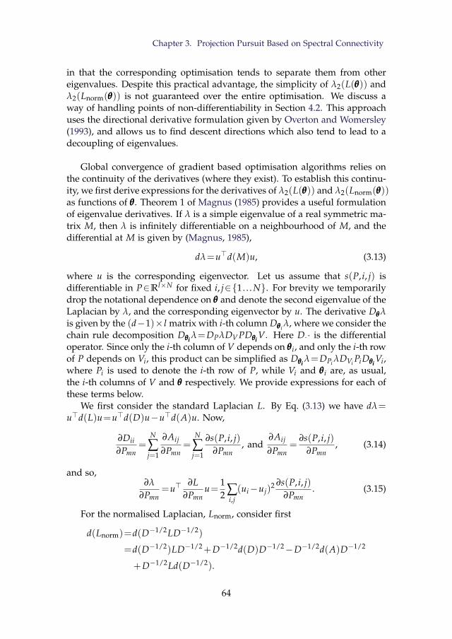
Chapter 3. Projection Pursuit Based on Spectral Connectivity
in that the corresponding optimisation tends to separate them from othereigenvalues. Despite this practical advantage, the simplicity of λ2(L(θθθ)) andλ2(Lnorm(θθθ)) is not guaranteed over the entire optimisation. We discuss away of handling points of non-differentiability in Section 4.2. This approachuses the directional derivative formulation given by Overton and Womersley(1993), and allows us to find descent directions which also tend to lead to adecoupling of eigenvalues.
Global convergence of gradient based optimisation algorithms relies onthe continuity of the derivatives (where they exist). To establish this continu-ity, we first derive expressions for the derivatives of λ2(L(θθθ)) and λ2(Lnorm(θθθ))as functions of θθθ. Theorem 1 of Magnus (1985) provides a useful formulationof eigenvalue derivatives. If λ is a simple eigenvalue of a real symmetric ma-trix M, then λ is infinitely differentiable on a neighbourhood of M, and thedifferential at M is given by (Magnus, 1985),
dλ=u>d(M)u, (3.13)
where u is the corresponding eigenvector. Let us assume that s(P, i, j) isdifferentiable in P∈Rl×N for fixed i, j∈1. . . N. For brevity we temporarilydrop the notational dependence on θθθ and denote the second eigenvalue of theLaplacian by λ, and the corresponding eigenvector by u. The derivative Dθθθλis given by the (d−1)× l matrix with i-th column Dθθθi
λ, where we consider thechain rule decomposition Dθiθiθi
λ=DPλDV PDθiθiθiV. Here D·· is the differential
operator. Since only the i-th column of V depends on θθθi, and only the i-th rowof P depends on Vi, this product can be simplified as Dθiθiθi
λ=DPi λDVi PiDθiθiθiVi,
where Pi is used to denote the i-th row of P, while Vi and θθθi are, as usual,the i-th columns of V and θθθ respectively. We provide expressions for each ofthese terms below.
We first consider the standard Laplacian L. By Eq. (3.13) we have dλ=u>d(L)u=u>d(D)u−u>d(A)u. Now,
∂Dii∂Pmn
=N
∑j=1
∂Aij
∂Pmn=
N
∑j=1
∂s(P, i, j)∂Pmn
, and∂Aij
∂Pmn=
∂s(P, i, j)∂Pmn
, (3.14)
and so,∂λ
∂Pmn=u>
∂L∂Pmn
u=12 ∑
i,j(ui−uj)
2 ∂s(P, i, j)∂Pmn
. (3.15)
For the normalised Laplacian, Lnorm, consider first
d(Lnorm)=d(D−1/2LD−1/2)
=d(D−1/2)LD−1/2+D−1/2d(D)D−1/2−D−1/2d(A)D−1/2
+D−1/2Ld(D−1/2).
64
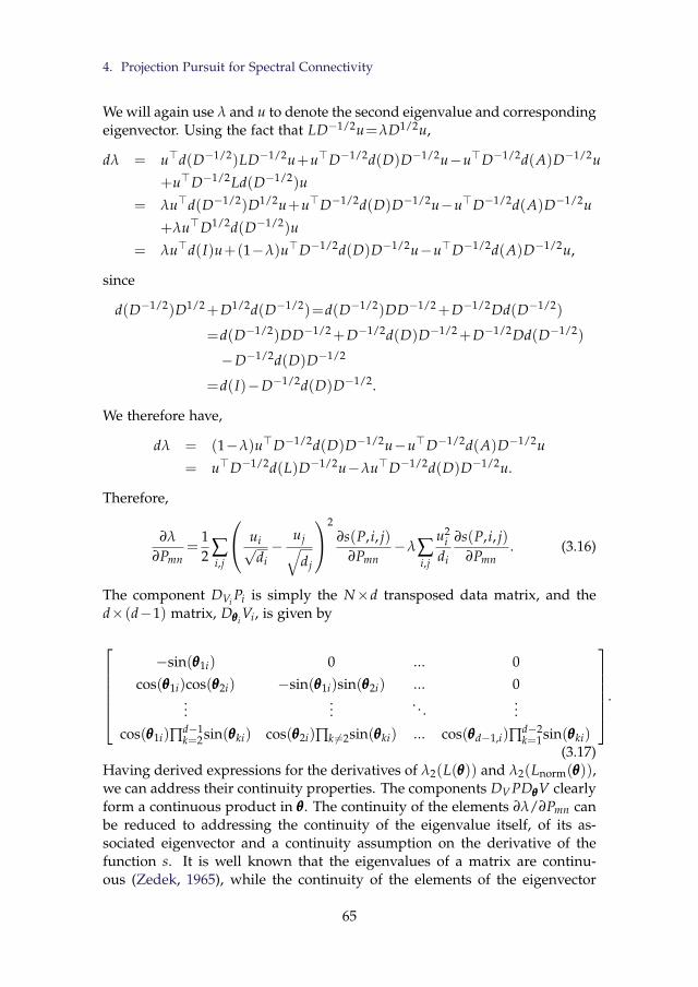
4. Projection Pursuit for Spectral Connectivity
We will again use λ and u to denote the second eigenvalue and correspondingeigenvector. Using the fact that LD−1/2u=λD1/2u,
dλ = u>d(D−1/2)LD−1/2u+u>D−1/2d(D)D−1/2u−u>D−1/2d(A)D−1/2u
+u>D−1/2Ld(D−1/2)u
= λu>d(D−1/2)D1/2u+u>D−1/2d(D)D−1/2u−u>D−1/2d(A)D−1/2u
+λu>D1/2d(D−1/2)u
= λu>d(I)u+(1−λ)u>D−1/2d(D)D−1/2u−u>D−1/2d(A)D−1/2u,
since
d(D−1/2)D1/2+D1/2d(D−1/2)=d(D−1/2)DD−1/2+D−1/2Dd(D−1/2)
=d(D−1/2)DD−1/2+D−1/2d(D)D−1/2+D−1/2Dd(D−1/2)
−D−1/2d(D)D−1/2
=d(I)−D−1/2d(D)D−1/2.
We therefore have,
dλ = (1−λ)u>D−1/2d(D)D−1/2u−u>D−1/2d(A)D−1/2u
= u>D−1/2d(L)D−1/2u−λu>D−1/2d(D)D−1/2u.
Therefore,
∂λ
∂Pmn=
12 ∑
i,j
ui√di−
uj√dj
2∂s(P, i, j)
∂Pmn−λ∑
i,j
u2i
di
∂s(P, i, j)∂Pmn
. (3.16)
The component DVi Pi is simply the N×d transposed data matrix, and thed×(d−1) matrix, Dθθθi
Vi, is given by
−sin(θθθ1i) 0 ... 0
cos(θθθ1i)cos(θθθ2i) −sin(θθθ1i)sin(θθθ2i) ... 0...
.... . .
...
cos(θθθ1i)∏d−1k=2sin(θθθki) cos(θθθ2i)∏k 6=2sin(θθθki) ... cos(θθθd−1,i)∏
d−2k=1sin(θθθki)
.
(3.17)Having derived expressions for the derivatives of λ2(L(θθθ)) and λ2(Lnorm(θθθ)),we can address their continuity properties. The components DV PDθθθV clearlyform a continuous product in θθθ. The continuity of the elements ∂λ/∂Pmn canbe reduced to addressing the continuity of the eigenvalue itself, of its as-sociated eigenvector and a continuity assumption on the derivative of thefunction s. It is well known that the eigenvalues of a matrix are continu-ous (Zedek, 1965), while the continuity of the elements of the eigenvector
65

Chapter 3. Projection Pursuit Based on Spectral Connectivity
come from the fact that we have assumed λ to be simple (Magnus, 1985). Weprovide full expressions for the derivatives of λ2(L(θθθ)) and λ2(Lnorm(θθθ)), forthe similarity function used in our experiments, in the Appendix.
The eigenvalues of a real, symmetric matrix can be expressed as the dif-ference between two convex matrix functions (Fan, 1949). If the similarityfunction, s, is Lipschitz continuous and differentiable we therefore have thatλ2(L(θθθ)) and λ2(Lnorm(θθθ)) are directionally differentiable everywhere. Over-ton and Womersley (1993) describe a way of expressing the directional deriva-tive of the sum of the k largest eigenvalues of a matrix whose elements arecontinuous functions of a parameter, at a point of non-simplicity of the k-thlargest eigenvalue. We will discuss the case of λ2(L(θθθ)), where λ2(Lnorm(θθθ))is analogous. If we denote the sum of the k largest eigenvalues of L(θθθ) byFk(θθθ) then,
λ2(L(θθθ))=FN−1(θθθ)−FN−2(θθθ). (3.18)
Now suppose that θθθ is such that
λN(L(θθθ))≥ ...≥λN−r+1(L(θθθ))>
λN−r(L(θθθ))= ...=λN−k+1(L(θθθ))= ...=λN−r−t+1(L(θθθ))>
λN−r−t(L(θθθ))≥ ...≥λ1(L(θθθ)).
That is, the k-th largest eigenvalue has multiplicity t and k−r are included inthe sum defining Fk(θθθ). Then the directional derivative of Fk(θθθ) in directionθ is given by (Overton and Womersley, 1993)
Fk′(θθθ;θ)=d−1
∑i=1
l
∑j=1
θijtrace(R>LijR)+ maxU∈Φt,k−r
d−1
∑i=1
l
∑j=1
θijtrace(Q>LijQU), (3.19)
where Lij=∂L(θθθ)/∂θθθij, the matrix R∈RN×r has j-th column equal to theeigenvector of the j-th largest eigenvalue of L(θθθ) and the matrix Q∈RN×t
has j-th column equal to the eigenvector of the (r+ j)-th largest eigenvalue ofL(θθθ). In addition the set Φa,b is defined as,
Φa,b :=U∈Sa|U and I−U are positive semi-definite and trace(U)=b.(3.20)
Overton and Womersley (1993) have shown that Fk′(θθθ;θ) is the sum of theeigenvalues of ∑d−1
i=1 ∑lj=1 θijR>LijR plus the sum of the k−r largest eigenval-
ues of ∑d−1i=1 ∑l
j=1 θijQ>LijQ. Therefore, the directional derivative of λ2(L(θθθ))
in the direction θ is given by the smallest eigenvalue of ∑d−1i=1 ∑l
j=1 θijQ>LijQ,where the matrix Q is constructed by any complete set of eigenvectors corre-sponding to the eigenvalue λ=λ2(L(θθθ)).
66
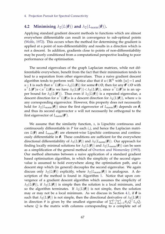
4. Projection Pursuit for Spectral Connectivity
4.2 Minimising λ2(L(θθθ)) and λ2(Lnorm(θθθ)).
Applying standard gradient descent methods to functions which are almosteverywhere differentiable can result in convergence to sub-optimal points(Wolfe, 1972). This occurs when the method for determining the gradient isapplied at a point of non-differentiability and results in a direction which isnot a descent. In addition, gradients close to points of non-differentiabilitymay be poorly conditioned from a computational perspective leading to poorperformance of the optimisation.
The second eigenvalues of the graph Laplacian matrices, while not dif-ferentiable everywhere, benefit from the fact that their minimisation tends tolead to a separation from other eigenvalues. Thus a naive gradient descentalgorithm tends to perform well. Notice also that if u∈RN with ‖u‖=1 andu⊥1 is such that u>L(θθθ)u=λ2(L(θθθ)) for some θθθ∈Θ, then for any θθθ′∈Θ withu>L(θθθ′)u<u>L(θθθ)u we have λ2(L(θθθ′))<λ2(L(θθθ)), since u>L(θθθ′)u is an up-per bound for λ2(L(θθθ′)). Thus even if λ2(L(θθθ)) is a repeated eigenvalue, adescent direction for u>L(θθθ)u is a descent direction for λ2(L(θθθ)), where u isany corresponding eigenvector. However, this property does not necessarilyhold for λ2(Lnorm(θθθ)) since the first eigenvector of Lnorm(θθθ) depends on θθθ,and thus its second eigenvector u will not necessarily be orthogonal to thefirst eigenvector of Lnorm(θθθ′).
We assume that the similarity function, s, is Lipschitz continuous andcontinuously differentiable in P for each i, j, and hence the Laplacian matri-ces L(θθθ) and Lnorm(θθθ) are element-wise Lipschitz continuous and continu-ously differentiable in θθθ. These conditions are sufficient for the everywheredirectional differentiability of λ2(L(θθθ)) and λ2(Lnorm(θθθ)). Our approach forfinding locally minimal solutions for λ2(L(θθθ)) and λ2(Lnorm(θθθ)) can be seenas a simplification of the general method of Overton and Womersley (1993).Our method alternates between a naive application of a standard gradientbased optimisation algorithm, in which the simplicity of the second eigen-value is assumed to hold everywhere along the optimisation path, and adescent step which (in general) decouples the second eigenvalue. We againdiscuss only λ2(L(θθθ)) explicitly, where λ2(Lnorm(θθθ)) is analogous. A de-scription of the method is found in Algorithm 1. Notice that upon con-vergence of a gradient descent algorithm which assumes the simplicity ofλ2(L(θθθ)), if λ2(L(θθθ)) is simple then the solution is a local minimum, andso the algorithm terminates. If λ2(L(θθθ)) is not simple, then the solutionmay or may not be a local minimum. As we discuss in Section 4.1, if θθθ issuch that λ2(L(θθθ)) is not simple, then the directional derivative of λ2(L(θθθ))in direction θ is given by the smallest eigenvalue of ∑d−1
i=1 ∑lj=1 θijQ>LijQ,
where Q is the matrix with columns corresponding to a complete set of
67
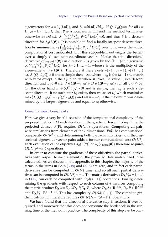
Chapter 3. Projection Pursuit Based on Spectral Connectivity
eigenvectors for λ=λ2(L(θθθ)), and Lij=∂L(θθθ)/∂θθθij. If Q>LijQ=0 for all i=1,...,d−1; j=1,..., l, then θθθ is a local minimum and the method terminates,otherwise ∃θ∈Θ s.t. λ1
(∑d−1
i=1 ∑lj=1 θijQ>LijQ
)<0, and thus θ is a descent
direction for λ2(L(θθθ)). It is possible to find a locally steepest descent direc-tion by minimising λ1
(1‖θ‖∑d−1
i=1 ∑lj=1 θijQ>LijQ
)over θ, however the added
computational cost associated with this subproblem outweighs the benefitover a simply chosen unit coordinate vector. Notice that the directionalderivative of λk+2(L(θθθ)) in direction θ is given by the (k+1)-th eigenvalueof ∑d−1
i=1 ∑lj=1 θijQ>LijQ, for k=0,1,...,t−1, where t is the multiplicty of the
eigenvalue λ=λ2(L(θθθ)). Therefore if there exists i∈1,...,d−1, j∈1,..., ls.t. λt(Q>LijQ)>0 and is simple then −eij, where −eij is the (d−1)× l matrixwith zeros except in the i, j-th entry where it takes the value 1, is a descentdirection and ∃γ>0 s.t. λ2(L(θθθ−γ′eij))<λ3(L(θθθ−γ′eij)) for all 0<γ′<γ.On the other hand if λ1(Q>LijQ)<0 and is simple, then eij is such a de-scent direction. If no such pair i, j exists, then we select i, j which maximisesmaxλt(Q>LijQ),−λ1(Q>LijQ) and set θ=−eij if the maximum was deter-mined by the largest eigenvalue and equal to eij otherwise.
Computational Complexity
Here we give a very brief discussion of the computational complexity of theproposed method. At each iteration in the gradient descent, computing theprojected dataset, P(θθθ), requires O(Nld) operations. Computing all pair-wise similarities from elements of the l-dimensional P(θθθ) has computationalcomplexity O(lN2), and determining both Laplacian matrices, and their as-sociated eigenvalue/vector pairs adds a further computational cost O(N2).Each evaluation of the objectives λ2(L(θθθ)) or λ2(Lnorm(θθθ)) therefore requiresO(lN(N+d)) operations.
In order to compute the gradients of these objectives, the partial deriva-tives with respect to each element of the projected data matrix need to becalculated. As we discuss in the appendix to this chapter, the majority of theterms in the sums in Eq.’s (3.15) and (3.16) are zero, and in fact each partialderivative can be computed in O(N) time, and so all such partial deriva-tives can be computed in O(lN2) time. The matrix derivatives Dθθθi
Vi, i=1,..., l,in (3.17) can each be computed with O(d(d−1)) operations. Finally, deter-mining the gradients with respect to each column of θθθ involves computingthe matrix product Dθθθi
λ=DPi λDVi PiDθθθiVi, where DPi λ∈R1×N , DVi Pi∈RN×d
and DθθθiVi∈Rd×(d−1). This has complexity O(Nd(d−1)). The complete gra-
dient calculation therefore requires O(lN(N+d(d−1))) operations.We have found that the directional derivative step is seldom, if ever re-
quired, and moreover that this does not constitute the bottleneck in the run-ning time of the method in practice. The complexity of this step can be com-
68

4. Projection Pursuit for Spectral Connectivity
Algorithm 1: Minimising λ2(L(θθθ))
1. Initialise θθθ.
2. Apply gradient based optimisation to λ2(L(θθθ)) assuming differentiability
3. ififif λ2(L(θθθ)) is simple thenthenthenreturnreturnreturn θθθ
4. Find Q∈RN×t, a complete set of t eigenvectors for eigenvalue λ=λ2(L(θθθ)).Find Lij=∂L(θθθ)/∂θθθij for i=1, . . . ,d−1, and j=1,..., l
5. ififif Q>LijQ=0 ∀i=1, . . . ,d−1; j=1,..., l thenthenthenreturnreturnreturn θθθ
6. ififif ∃i∈1, . . . ,d−1; j∈1,..., l s.t. λt(Q>LijQ)>0 and is simple thenthenthenθθθ←argminθθθ′λ2(L(θθθ′)) s.t. θθθ′=θθθ−γeij, γ>0, λ2(L(θθθ′)) is simplego togo togo to 2.
7. ififif ∃i∈1, . . . ,d−1; j∈1,..., l s.t. λ1(Q>LijQ)<0 and is simple thenthenthenθθθ←argminθθθ′λ2(L(θθθ′)) s.t. θθθ′=θθθ+γeij, γ>0, λ2(L(θθθ′)) is simplego togo togo to 2.
8. (I, J)←argmax(i,j)maxλt(Q>LijQ),−λ1(Q>LijQ)
9. ififif λt(Q>LI J Q)>−λ1(Q>LI J Q) thenthenthenθθθ←argminθθθ′λ2(L(θθθ′)) s.t. θθθ′=θθθ−γeI J ,γ>0go togo togo to 4.
10. θθθ←argminθθθ′λ2(L(θθθ′)) s.t. θθθ′=θθθ+γeI J ,γ>0go togo togo to 4.
11. endendend
puted along similar lines, and be found to be O(t2lN(N+d(d−1))), where tis the multiplicity of the eigenvalue λ=λ2(L(θθθ)).
The total complexity of the projection pursuit optimisation depends onthe number of iterations in the gradient descent method, where in generalthis number is bounded for a given accuracy level. For our experiments weuse the BFGS (Broyden-Fletcher-Goldfarb-Shanno) algorithm as this has beenfound to perform well even on non-smooth functions (Lewis and Overton,2013).
4.3 Computing Similarities
It is common to define pairwise similarities of points via a decreasing func-tion of the distance between them. That is, for a decreasing function k :R+→R+, the similarity function s may be written,
s(P, i, j)=k(d(pi, pj)
σ
), (3.21)
69
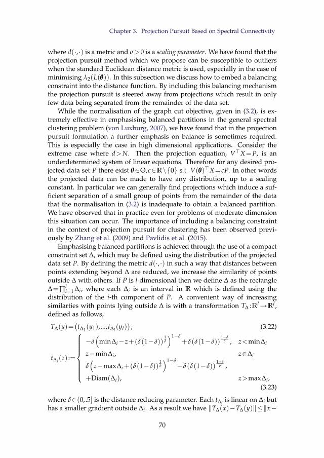
Chapter 3. Projection Pursuit Based on Spectral Connectivity
where d(·, ·) is a metric and σ>0 is a scaling parameter. We have found that theprojection pursuit method which we propose can be susceptible to outlierswhen the standard Euclidean distance metric is used, especially in the case ofminimising λ2(L(θθθ)). In this subsection we discuss how to embed a balancingconstraint into the distance function. By including this balancing mechanismthe projection pursuit is steered away from projections which result in onlyfew data being separated from the remainder of the data set.
While the normalisation of the graph cut objective, given in (3.2), is ex-tremely effective in emphasising balanced partitions in the general spectralclustering problem (von Luxburg, 2007), we have found that in the projectionpursuit formulation a further emphasis on balance is sometimes required.This is especially the case in high dimensional applications. Consider theextreme case where d>N. Then the projection equation, V>X=P, is anunderdetermined system of linear equations. Therefore for any desired pro-jected data set P there exist θθθ∈Θ,c∈R\0 s.t. V(θθθ)>X=cP. In other wordsthe projected data can be made to have any distribution, up to a scalingconstant. In particular we can generally find projections which induce a suf-ficient separation of a small group of points from the remainder of the datathat the normalisation in (3.2) is inadequate to obtain a balanced partition.We have observed that in practice even for problems of moderate dimensionthis situation can occur. The importance of including a balancing constraintin the context of projection pursuit for clustering has been observed previ-ously by Zhang et al. (2009) and Pavlidis et al. (2015).
Emphasising balanced partitions is achieved through the use of a compactconstraint set ∆, which may be defined using the distribution of the projecteddata set P. By defining the metric d(·, ·) in such a way that distances betweenpoints extending beyond ∆ are reduced, we increase the similarity of pointsoutside ∆ with others. If P is l dimensional then we define ∆ as the rectangle∆=∏l
i=1 ∆i, where each ∆i is an interval in R which is defined using thedistribution of the i-th component of P. A convenient way of increasingsimilarties with points lying outside ∆ is with a transformation T∆ :Rl→Rl ,defined as follows,
T∆(y)=(t∆1(y1), ...,t∆l (yl)
), (3.22)
t∆i (z) :=
−δ(
min∆i−z+(δ(1−δ))1δ
)1−δ+δ(δ(1−δ))
1−δδ , z<min∆i
z−min∆i, z∈∆i
δ(
z−max∆i+(δ(1−δ))1δ
)1−δ−δ(δ(1−δ))
1−δδ ,
+Diam(∆i), z>max∆i,(3.23)
where δ∈(0,.5] is the distance reducing parameter. Each t∆i is linear on ∆i buthas a smaller gradient outside ∆i. As a result we have ‖T∆(x)−T∆(y)‖≤‖x−
70
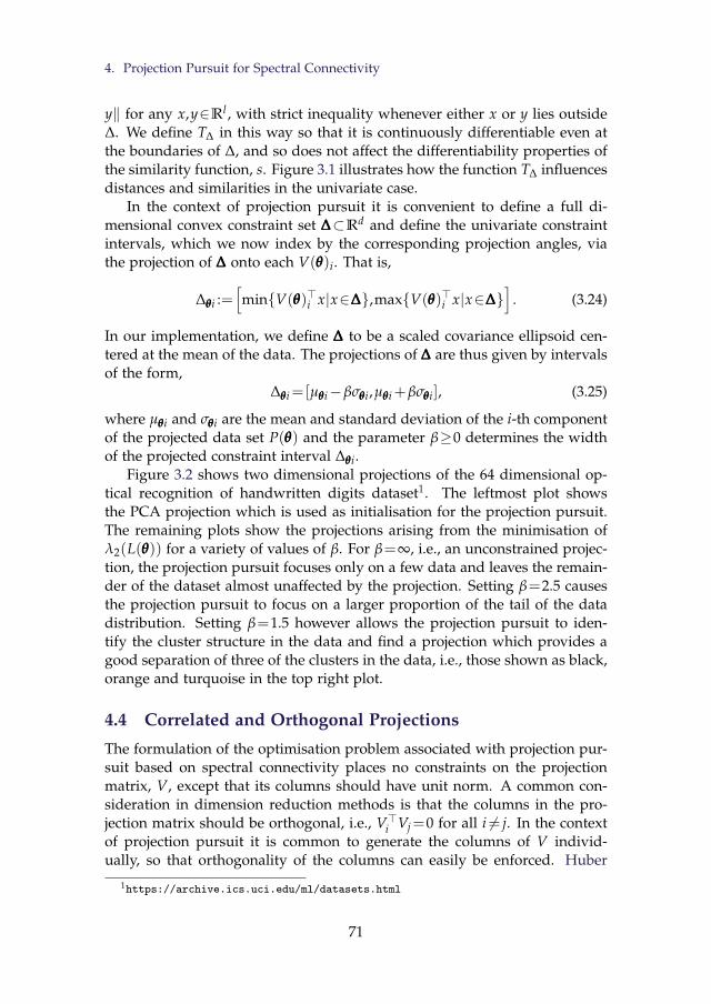
4. Projection Pursuit for Spectral Connectivity
y‖ for any x,y∈Rl , with strict inequality whenever either x or y lies outside∆. We define T∆ in this way so that it is continuously differentiable even atthe boundaries of ∆, and so does not affect the differentiability properties ofthe similarity function, s. Figure 3.1 illustrates how the function T∆ influencesdistances and similarities in the univariate case.
In the context of projection pursuit it is convenient to define a full di-mensional convex constraint set ∆∆∆⊂Rd and define the univariate constraintintervals, which we now index by the corresponding projection angles, viathe projection of ∆∆∆ onto each V(θθθ)i. That is,
∆θθθi :=[minV(θθθ)>i x|x∈∆∆∆,maxV(θθθ)>i x|x∈∆∆∆
]. (3.24)
In our implementation, we define ∆∆∆ to be a scaled covariance ellipsoid cen-tered at the mean of the data. The projections of ∆∆∆ are thus given by intervalsof the form,
∆θθθi=[µθθθi−βσθθθi,µθθθi+βσθθθi], (3.25)
where µθθθi and σθθθi are the mean and standard deviation of the i-th componentof the projected data set P(θθθ) and the parameter β≥0 determines the widthof the projected constraint interval ∆θθθi.
Figure 3.2 shows two dimensional projections of the 64 dimensional op-tical recognition of handwritten digits dataset1. The leftmost plot showsthe PCA projection which is used as initialisation for the projection pursuit.The remaining plots show the projections arising from the minimisation ofλ2(L(θθθ)) for a variety of values of β. For β=∞, i.e., an unconstrained projec-tion, the projection pursuit focuses only on a few data and leaves the remain-der of the dataset almost unaffected by the projection. Setting β=2.5 causesthe projection pursuit to focus on a larger proportion of the tail of the datadistribution. Setting β=1.5 however allows the projection pursuit to iden-tify the cluster structure in the data and find a projection which provides agood separation of three of the clusters in the data, i.e., those shown as black,orange and turquoise in the top right plot.
4.4 Correlated and Orthogonal Projections
The formulation of the optimisation problem associated with projection pur-suit based on spectral connectivity places no constraints on the projectionmatrix, V, except that its columns should have unit norm. A common con-sideration in dimension reduction methods is that the columns in the pro-jection matrix should be orthogonal, i.e., V>i Vj=0 for all i 6= j. In the contextof projection pursuit it is common to generate the columns of V individ-ually, so that orthogonality of the columns can easily be enforced. Huber
1https://archive.ics.uci.edu/ml/datasets.html
71
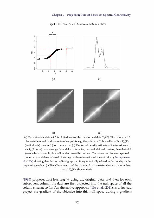
Chapter 3. Projection Pursuit Based on Spectral Connectivity
Fig. 3.1: Effect of T∆ on Distances and Similarities.
−5 0 5 10 15 20
−10
−5
05
1015
20
P
T(P
)
(a) (b)
(c) (d)
(a) The univariate data set P is plotted against the transformed data T∆(P). The point at ≈15
lies outside ∆ and its distance to other points, e.g. the point at ≈2, is smaller within T∆(P)
(vertical axis) than in P (horizontal axis). (b) The kernel density estimate of the transformed
data T∆(P) (- - -) has a stronger bimodal structure, i.e., two well defined clusters, than that of P
(—–), which has multiple small modes caused by outliers. The connection between spectral
connectivity and density based clustering has been investigated theoretically by Narayanan et
al. (2006) showing that the normalised graph cut is asymptotically related to the density on the
separating surface. (c) The affinity matrix of the data set P has a weaker cluster structure than
that of T∆(P), shown in (d).
(1985) proposes first learning V1 using the original data, and then for eachsubsequent column the data are first projected into the null space of all thecolumns learnt so far. An alternative approach (Niu et al., 2011), is to insteadproject the gradient of the objective into this null space during a gradient
72
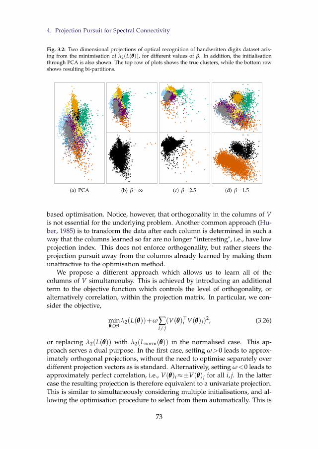
4. Projection Pursuit for Spectral Connectivity
Fig. 3.2: Two dimensional projections of optical recognition of handwritten digits dataset aris-ing from the minimisation of λ2(L(θθθ)), for different values of β. In addition, the initialisationthrough PCA is also shown. The top row of plots shows the true clusters, while the bottom rowshows resulting bi-partitions.
(a) PCA
x[,1]
(b) β=∞
x[,1]
(c) β=2.5
x[,1]
(d) β=1.5
based optimisation. Notice, however, that orthogonality in the columns of Vis not essential for the underlying problem. Another common approach (Hu-ber, 1985) is to transform the data after each column is determined in such away that the columns learned so far are no longer “interesting", i.e., have lowprojection index. This does not enforce orthogonality, but rather steers theprojection pursuit away from the columns already learned by making themunattractive to the optimisation method.
We propose a different approach which allows us to learn all of thecolumns of V simultaneoulsy. This is achieved by introducing an additionalterm to the objective function which controls the level of orthogonality, oralternatively correlation, within the projection matrix. In particular, we con-sider the objective,
minθθθ∈Θ
λ2(L(θθθ))+ω∑i 6=j
(V(θθθ)>i V(θθθ)j)2, (3.26)
or replacing λ2(L(θθθ)) with λ2(Lnorm(θθθ)) in the normalised case. This ap-proach serves a dual purpose. In the first case, setting ω>0 leads to approx-imately orthogonal projections, without the need to optimise separately overdifferent projection vectors as is standard. Alternatively, setting ω<0 leads toapproximately perfect correlation, i.e., V(θθθ)i≈±V(θθθ)j for all i, j. In the lattercase the resulting projection is therefore equivalent to a univariate projection.This is similar to simultaneously considering multiple initialisations, and al-lowing the optimisation procedure to select from them automatically. This is
73
Chapter 3. Projection Pursuit Based on Spectral Connectivity
important as the objectives λ2(L(θθθ)) and λ2(Lnorm(θθθ)) are non-convex, andas a result applying gradient based optimisation can only guarantee conver-gence to a local optimum.
Notice also that the formulation in Eq. (3.26) offers computational benefitsover the alternative of optimising separately over each projection vector, sincethe eigenvalues/vectors computed in each function and gradient evaluationneed only be computed once for each iteration over the multiple projectiondimensions.
5 Connection with Maximal Margin Hyperplanes
In this section we establish a connection between the optimal univariate pro-jection for spectral bi-partitioning using the standard Laplacian and largemargin separators. In particular, under suitable conditions, as the scalingparameter tends to zero the optimal projection for spectral bi-partitioningconverges to the vector admitting the largest margin hyperplane through thedata. This establishes a theoretical connection between spectral connected-ness and separability of the resulting clusters in terms of Euclidean distance.Large margin separators are ubiquitous in the machine learning literature,and were first introduced in the context of supervised classification via sup-port vector machines (SVM, Vapnik and Kotz (1982)). In more recent yearsthey have shown to be very useful for unsupervised partitioning in the con-text of maximum margin clustering as well (Xu et al., 2004; Zhang et al.,2009).
Our result pertains to univariate projections, and therefore the d×1 pro-jection matrix is equivalently viewed as a projection vector in Rd. We thereforeuse the notation v(θθθ), instead of V(θθθ) as before.
The result holds for all similarities for which the function k, in Eq. (3.21),satisfies the tail condition limx→∞ k(x+ε)/k(x)=0 for all ε>0. This condi-tions is satisfied by functions with exponentially decaying tails, including thepopular Gaussian and Laplace kernels. It is, however, not satisfied by thosewith polynomially decaying tails.
The constraint set ∆∆∆ again plays an important role as in many cases thelargest margin hyperplane through a set of data separates only a few pointsfrom the rest, making it meaningless for the purpose of clustering. We there-fore prefer to restrict the hyperplane to intersect the set ∆∆∆. What we in factshow in this section is that there exists a set ∆∆∆′⊂∆∆∆ satisfying ∆∆∆′∩X=∆∆∆∩X,such that, as the scaling parameter tends to zero, the optimal projection forλ2(L(θθθ)) converges to the projection admitting the largest margin hyperplanethat intersects ∆∆∆′. The distinction between the largest margin hyperplane in-tersecting ∆∆∆′ and that intersecting ∆∆∆ is scarcely of practical relevance, butplays an important role in the theory we present in this section. It accounts
74
5. Connection with Maximal Margin Hyperplanes
for situations when the largest margin hyperplane intersecting ∆∆∆ lies close toits boundary and the distance between the hyperplane and the nearest pointoutside ∆∆∆ is larger than to the nearest point inside ∆∆∆. Aside from this veryspecific case, the two in fact coincide.
A hyperplane is a translated subspace of co-dimension 1, and can be pa-rameterised by a non-zero vector v∈Rd\0 and scalar b as the set H(v,b)=x∈Rd
∣∣v>x=b. Clearly, for any c∈R\0, one has H(v,b)=H(cv,cb), andso we can assume that v has unit norm, thus the same parameterisation byθθθ can be used. For a finite set of points X⊂Rd, the margin of hyperplaneH(v(θθθ),b) w.r.t. X is the minimal Euclidean distance between H(v(θθθ),b) andX. That is,
margin(v(θθθ),b)=minx∈X|v(θθθ)>x−b|. (3.27)
Connections between maximal margin hyperplanes and Bayes optimal hy-perplanes as well as minimum density hyperplanes have been established(Tong and Koller, 2000; Pavlidis et al., 2015).
In this section we use the notation v>X=v>x1, ...,v>xN, and for a set P⊂R
and y∈R we write, for example, P>y for P∩(y,∞). For scaling parameter σ>0 and distance reduction factor δ>0 we define θθθσ,δ :=argminθθθ∈Θλ2(L(θθθ,σ,δ)),where L(θθθ,σ,δ) is as L(θθθ) from before, but with an explicit dependence onthe scaling parameter and distance reducing parameter used in the similarityfunction. That is, θθθσ,δ defines the projection generating the minimal spectralconnectivity of X for a given pair σ,δ.
Before proving the main result of this section, we require the following sup-porting results. Lemma 11 provides a lower bound on the second eigenvalueof the graph Laplacian of a one dimensional data set in terms of the largestEuclidean separation of adjacent points, with respect to a constraint set ∆.This lemma also shows how we construct the set ∆∆∆′. Lemma 12 uses this re-sult to show that a projection angle θθθ∈Θ leads to lower spectral connectivitythan all projections admitting smaller maximal margin hyperplanes intersect-ing ∆∆∆′ for all pairs σ,δ sufficiently close to zero.
Lemma 11 Let k :R+→R+ be a non-increasing, positive function and let σ>0,δ∈(0,0.5]. Let P=p1, ..., pN be a univariate data set and let ∆=[a,b] for a<b∈R.Suppose that |P∩∆|≥2 and a≥minP,b≤maxP. Define ∆′=[a′,b′], wherea′=(a+minP∩∆)/2, b′=(b+maxP∩∆)/2. Let M=maxx∈∆′mini=1...N|x− pi|. Define L(P) to be the Laplacian of the graph with vertices P and similari-ties according to s(P, i, j)=k(|T∆(pi)−T∆(pj)|/σ). Then λ2(L(P))≥ 1
|P|3 k((2M+
δC)/σ), where C=maxD,D1−δ, D=maxa−minP,maxP−b.
Proof We can assume that P is sorted in increasing order, i.e. pi≤ pi+1, sincethis does not affect the eigenvalues of L(P). We first show that s(P, i, i+1)≥
75
Chapter 3. Projection Pursuit Based on Spectral Connectivity
k((2M+δC)/σ) for all i=1,..., N−1. To this end observe that for x≥0 we
have δ(
x+(
δ(1−δ)1δ
))1−δ−δ(δ(1−δ))
1−δδ ≤δmaxx,x1−δ.
• If pi, pi+1≤a then s(P, i, i+1)=k((T∆(pi+1)−T∆(pi))/σ) ≥k((T∆(a)−T∆(pi))/σ) ≥k((2M+δC)/σ) by the definition of C and using the aboveinequality, since k is non-increasing. The case pi, pi+1≥b is similar.
• If pi, pi+1∈∆ then pi, pi+1∈∆′⇒|pi− pi+1|≤2M⇒s(P, i, i+1)≥k(2M/σ)≥k((2M+δC)/σ) since M is the largest margin in ∆′.
• If none the above hold, then we lose no generality in assuming pi<a, a< pi+1<b since the case a< pi<b, pi+1>b is analogous. We musthave pi+1=minP∩∆ and so a′=(a+ pi+1)/2. If pi+1−a>2M thenminj=1...N |a′− pj|>M, a contradiction since a′∈∆′ and M is the largestmargin in ∆′. Therefore pi+1−a≤2M. In all T∆(pi+1)−T∆(pi)=(pi+1−a)+δ(a− pi+(δ(1−δ))
1δ )1−δ−δ(δ(1−δ))
1−δδ ≤2M+δC⇒s(P, i, i+1)≥
k((2M+δC)/σ).
Now, let u be the second eigenvector of L(P). Then ‖u‖=1 and u⊥1 andtherefore ∃i, j s.t. ui−uj≥ 1√
|P|. We thus know that there exists m s.t. |um−
um+1|≥ 1|P|3/2 . By (von Luxburg, 2007, Proposition 1), we know that u>L(P)u=
12 ∑i,j s(P, i, j)(ui−uj)
2≥s(P,m,m+1)(um−um+1)2≥ 1|P|3 k((2M+δC)/σ) since
all consecutive pairs pm, pm+1 have similarity at least k((2M+δC)/σ), byabove. Therefore λ2(L(P))≥ 1
|P|3 k((2M+δC)/σ) as required.
In the above Lemma we have assumed that ∆ is contained within theconvex hull of the points P, however the results of this section can easilybe modified to allow for cases where this does not hold. In particular, ifan unconstrained large margin hyperplane is sought, then setting ∆∆∆ to bearbitrarily large allows for this. We have merely stated the results in the mostconvenient context for our practical implementation.
The set ∆′ in the above is defined in terms of the one dimensional con-straint set [a,b]. We define the full dimensional set ∆∆∆′ along the same linesby,
∆∆∆′ :=x∈Rd|v(θθθ)>x∈∆′θθθ ∀θθθ∈Θ,
∆′θθθ =
[min∆θθθ +minv(θθθ)>X∩∆θθθ
2,max∆θθθ +maxv(θθθ)>X∩∆θθθ
2
]. (3.28)
Here we assume that ∆∆∆ is contained within the convex hull of the d-dimensionaldata set X. Notice that since ∆∆∆ is convex, we have v(θθθ)>∆∆∆′=∆′θθθ . In what fol-lows we show that as σ and δ are reduced to zero the optimal projection forspectral partitioning converges to the projection admitting the largest margin
76
5. Connection with Maximal Margin Hyperplanes
hyperplane intersecting ∆∆∆′. If it is the case that the largest margin hyper-plane intersecting ∆∆∆ also intersects ∆∆∆′, as is often the case, although thisfact will not be known, then it is actually not necessary that δ tend towardszero. In such cases it only needs to satisfy δ≤2M/C for the correspond-ing values of M and C over all possible projections. In particular, choosingmaxDiam(X),Diam(X)1−δ instead of C is appropriate for all projections.
Lemma 12 Let θθθ∈Θ and let k :R+→R+ be non-increasing, positive, and satisfy
limx→∞
k(x(1+ε))/k(x)=0
for all ε>0. Then for any 0<m<maxb∈∆′θθθ
margin(v(θθθ),b) there exists σ′>0 andδ′>0 s.t. 0<σ<σ′, 0<δ<δ′ and maxc∈∆′
θθθ′margin(v(θθθ′),c)<maxb∈∆′
θθθmargin(v(θθθ),
b)−m⇒λ2(L(θθθ,σ,δ))<λ2(L(θθθ′,σ,δ)).
Proof Let B=argmaxb∈∆′θθθmargin(v(θθθ),b) and M=margin(v(θθθ),B). We as-
sume that M 6=0, since otherwise there is nothing to show. Now, since spec-tral clustering solves a relaxation of the minimum normalised cut problemwe have,
λ2(L(θθθ,σ,δ))≤ 1|X|min
C⊂X∑
i,j:xi∈Cxj 6∈C
s(P(θθθ), i, j)(
1|C|+
1|X\C|
)
≤ 1|X| ∑
i,j:v(θθθ)>xi<Bv(θθθ)>xj>B
s(P(θθθ), i, j)(
1|(v(θθθ)>X)<B|
+1
|(v(θθθ)>X)>B|
)
=1|X| ∑
i,j:v(θθθ)>xi<Bv(θθθ)>xj>B
k
(T∆θθθ
(v(θθθ)>xj)−T∆θθθ(v(θθθ)>xi)
σ
)
×(
|X||(v(θθθ)>X)<B||(v(θθθ)>X)>B|
)≤∣∣(v(θθθ)>X)<B
∣∣∣∣(v(θθθ)>X)>B∣∣k(2M
σ
)(1
|(v(θθθ)>X)<B||(v(θθθ)>X)>B|
)=k(2M/σ).
The final inequality holds since for any i, j s.t. v(θθθ)>xi<B and v(θθθ)>xj>Bwe must have T∆θθθ
(v(θθθ)>xj)−T∆θθθ(v(θθθ)>xi)≥2M. Now, for any θθθ′∈Θ, let
Mθθθ′=maxc∈∆′θθθ′
margin(v(θθθ′),c). By Lemma 11 we know that λ2(L(θθθ′,σ,δ))≥
77
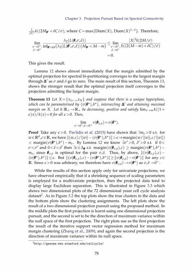
Chapter 3. Projection Pursuit Based on Spectral Connectivity
1|X|3 k((2Mθθθ′+δC/σ), where C=maxDiam(X), Diam(X)1−δ. Therefore,
limσ→0+ ,δ→0+
λ2(L(θθθ,σ,δ))infθθθ′∈Θλ2(L(θθθ′,σ,δ))
∣∣Mθθθ′<M−m≤ lim
σ→0+ ,δ→0+
|X|3k(2M/σ)
k((2(M−m)+δC)/σ)
=0.
This gives the result.
Lemma 12 shows almost immediately that the margin admitted by theoptimal projection for spectral bi-partitioning converges to the largest marginthrough ∆∆∆′ as σ and δ go to zero. The main result of this section, Theorem 13,shows the stronger result that the optimal projection itself converges to theprojection admitting the largest margin.
Theorem 13 Let X=x1, ...,xN and suppose that there is a unique hyperplane,which can be parameterised by (v(θθθ?),b?), intersecting ∆∆∆′ and attaining maximalmargin on X. Let k :R+→R+ be decreasing, positive and satisfy limx→∞ k((1+ε)x)/k(x)=0 for all ε>0. Then,
limσ→0+ ,δ→0+
v(θθθσ,δ)=v(θθθ?).
Proof Take any ε>0. Pavlidis et al. (2015) have shown that ∃mε>0 s.t. forw∈Rd,c∈R, we have ‖(w,c)/‖w‖−(v(θθθ?),b?)‖>ε⇒margin(w/‖w‖,c/‖w‖)< margin(v(θθθ?),b?)−mε. By Lemma 12 we know ∃σ′>0, δ′>0 s.t. if 0<σ<σ′ and 0<δ<δ′ then ∃c∈∆θθθ s.t. margin(v(θθθσ,δ),c) ≥ margin(v(θθθ?),b?)−mε, since θθθσ,δ is optimal for the pair σ,δ. Thus, by above, ‖(v(θθθσ,δ),c)−(v(θθθ?),b?)‖≤ε. But ‖(v(θθθσ,δ),c)−(v(θθθ?),b?)‖≥‖v(θθθσ,δ)−v(θθθ?)‖ for any c∈R. Since ε>0 was arbitrary, we therefore have v(θθθσ,δ)→v(θθθ?) as σ,δ→0+.
While the results of this section apply only for univariate projections, wehave observed empirically that if a shrinking sequence of scaling parametersis employed for a multivariate projection, then the projected data tend todisplay large Euclidean separation. This is illustrated in Figure 3.3 whichshows two dimensional plots of the 72 dimensional yeast cell cycle analysisdataset2. As in Figure 3.2 the top plots show the true clusters in the data andthe bottom plots show the clustering assignments. The left plots show theresult of a two dimensional projection pursuit using the proposed method. Inthe middle plots the first projection is learnt using one dimensional projectionpursuit, and the second is set to be the direction of maximum variance withinthe null space of the first projection. The right plots use as the first projectionthe result of the iterative support vector regression method for maximummargin clustering (Zhang et al., 2009), and again the second projection is thedirection of maximum variance within its null space.
2http://genome-www.stanford.edu/cellcycle/
78
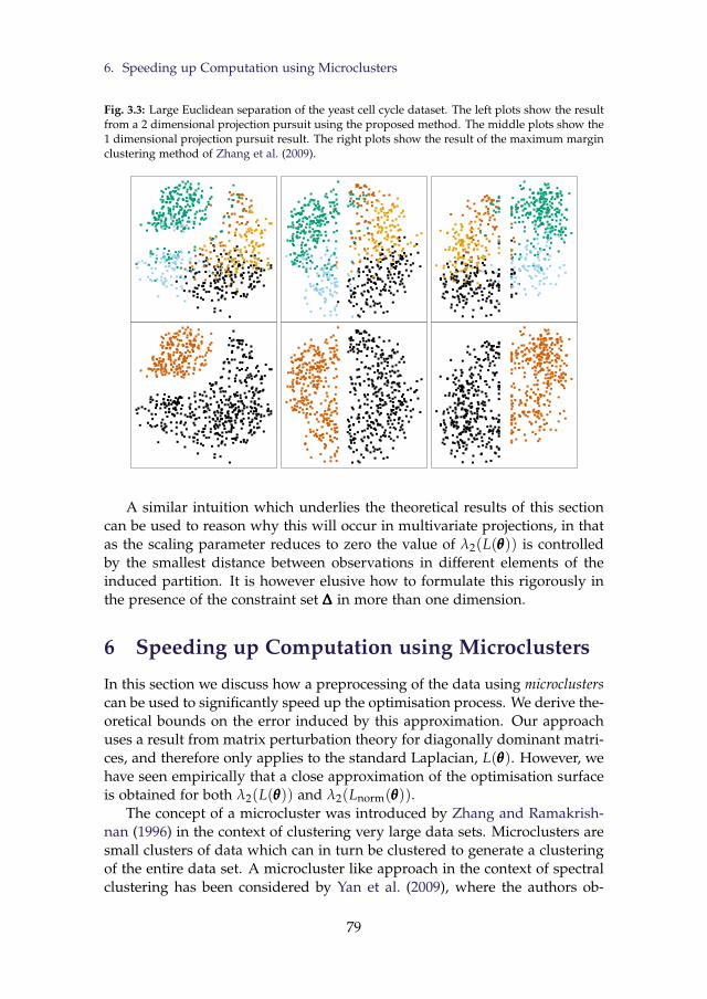
6. Speeding up Computation using Microclusters
Fig. 3.3: Large Euclidean separation of the yeast cell cycle dataset. The left plots show the resultfrom a 2 dimensional projection pursuit using the proposed method. The middle plots show the1 dimensional projection pursuit result. The right plots show the result of the maximum marginclustering method of Zhang et al. (2009).
x[,1]
A similar intuition which underlies the theoretical results of this sectioncan be used to reason why this will occur in multivariate projections, in thatas the scaling parameter reduces to zero the value of λ2(L(θθθ)) is controlledby the smallest distance between observations in different elements of theinduced partition. It is however elusive how to formulate this rigorously inthe presence of the constraint set ∆∆∆ in more than one dimension.
6 Speeding up Computation using Microclusters
In this section we discuss how a preprocessing of the data using microclusterscan be used to significantly speed up the optimisation process. We derive the-oretical bounds on the error induced by this approximation. Our approachuses a result from matrix perturbation theory for diagonally dominant matri-ces, and therefore only applies to the standard Laplacian, L(θθθ). However, wehave seen empirically that a close approximation of the optimisation surfaceis obtained for both λ2(L(θθθ)) and λ2(Lnorm(θθθ)).
The concept of a microcluster was introduced by Zhang and Ramakrish-nan (1996) in the context of clustering very large data sets. Microclusters aresmall clusters of data which can in turn be clustered to generate a clusteringof the entire data set. A microcluster like approach in the context of spectralclustering has been considered by Yan et al. (2009), where the authors ob-
79
Chapter 3. Projection Pursuit Based on Spectral Connectivity
tain bounds on the mis-clustering rate induced by the approximation. Ratherthan using microclusters as an intermediate step towards determining a finalclustering model, we use them to form an approximation of the optimisa-tion surface for projection pursuit which is less computationally expensive toexplore. The error bound depends on the ratio of cluster radii to scaling pa-rameter. As such, this method does not provide a good approximation whenσ is close to zero. Our bounds rely on the following result from perturbationtheory.
Theorem 14 Ye (2009)Let A=[aij] and A=[aij] be two symmetric positive semidefinite diagonally dom-inant matrices, and let λ1≤λ2≤ ...≤λn and λ1≤ λ2≤ ...≤ λn be their respectiveeigenvalues. If, for some 0≤ε<1, |aij− aij|≤ε|aij| ∀i 6= j, and |vi− vi|≤εvi ∀i,where vi=aii−∑j 6=i |aij|, and similarly for vi, then
|λi− λi|≤ελi ∀i.
An inspection of the proof of Theorem 14 reveals that ε<1 is necessary onlyto ensure that the signs of aij are the same as those of aij. In the case ofLaplacian matrices this equivalence of signs holds by design, and so in thiscontext the requirement that ε<1 can be relaxed.
In the microcluster approach, the data set X=x1, ...,xN is replaced withK points c1, ...,cK which represent the centers of a K-clustering of X. By pro-jecting these microcluster centers during subspace optimisation, rather thanthe data themselves, the computational cost associated with each eigen prob-lem is reduced from O(N2) to O(K2). If we define the radius, ρ, of a clusterC to be the greatest distance between one of its members and its center, thatis,
ρ(C)=maxx∈C
∥∥∥∥∥x− 1|C| ∑
x∈Cx
∥∥∥∥∥ , (3.29)
then we expect the approximation error to be small whenever the microclus-ter radii are small. The bounds on the approximation error which we presentin this section are worst case and rely on standard eigenvalue bounds, andso can be pessimistic. To obtain a reasonable bound on the approximationsurface, as many as K≈0.6N might be needed, leading to only a threefoldspeed up. We have observed empirically, however, that even for K=0.1N(and sometimes lower) one still obtains a close approximation of the optimi-sation surface. This makes the projection pursuit of the order of 100 timesfaster.
Lemma 15 Let C=C1, ...,CK be a K-clustering of X with centers c1, ...,cK, radiiρ1, ...,ρK and counts n1, ...,nK. For θθθ∈Θ define N(θθθ),B(θθθ)∈RK×K where N(θθθ) is
80
6. Speeding up Computation using Microclusters
the diagonal matrix with
N(θθθ)i,i=K
∑j=1
njs(Pc(θθθ), i, j)
andB(θθθ)i,j=
√ninjs(Pc(θθθ), i, j),
where Pc(θθθ)=V(θθθ)>c1, ...,V(θθθ)>cK are the projected microcluster centers andthe similarities are given by s(Pc(θθθ), i, j)=k(‖T∆θθθ
(V(θθθ)>ci)−T∆θθθ(V(θθθ)>cj)‖/σ),
and k(x) is positive and non-increasing for x≥0. Then,
|λ2(L(θθθ))−λ2(N(θθθ)−B(θθθ))|λ2(L(θθθ))
≤maxi 6=j
max
1−
k(Dij/σ)
k((Dij−ρi−ρj)+/σ),
k(Dij/σ)
k((Dij+ρi+ρj)/σ)−1
,
where Dij=‖T∆θθθ(V(θθθ)>ci)−T∆θθθ
(V(θθθ)>cj)‖ and (x)+=max0,x.
Proof For brevity we temporarily drop the notational dependence on θθθ. LetPc′=V>c1,V>c1, ...,V>cK,V>cK, where each V>ci is repeated ni times. LetLc′ be the Laplacian of the graph with vertices Pc′ and edges given by s(Pc′, i, j).We begin by showing that λ2(Lc′)=λ2(N−B). Take v∈RK, then,
v>(N−B)v=∑i,j
s(Pc, i, j)(v2i nj−vivj
√ninj)
=12 ∑
i,js(Pc, i, j)(v2
i nj+v2j ni−2vivj
√ninj)
≥0,
and so N−B is positive semi-definite. In addition, it is straightforward toverify that (N−B)(
√n1 . . .
√nK)=0, and hence 0 is the smallest eigenvalue
of N−B with eigenvector (√
n1 . . .√
nK). Now, let u be the second eigen-vector of Lc′. Then uj=uk for pairs of indices j,k aligned with the same V>ci
in Pc′. Define uc∈RK s.t. uci =√
niuj where index j is aligned with V>ci
in Pc′j . Then (uc)>(
√n1 . . .
√nK)=∑K
i=1 uci√
ni=∑Ki=1 niuji where index ji is
aligned with V>ci in Pc′ji
for each i. Therefore niuji =∑j:Pc′=V>ciuj and hence
(uc)>(√
n1 . . .√
nK)=∑Ki=1 ∑j:Pc′
j =V>ciuj=∑N
i=1 ui=0 since 1 is the smallest
eigenvector of Lc′ and so u⊥1. Similarly ‖uc‖2=∑Ki=1 niu2
ji=∑N
i=1 u2i =1. Thus
uc⊥(√
n1 . . .√
nK) and ‖uc‖=1 and so is a candidate for the second eigen-vector of N−B. In addition it is straightforward to show that (uc)>(N−B)uc=u ·Lc′u. Now, suppose by way of contradiction that ∃w⊥(
√n1 . . .
√nK)
81

Chapter 3. Projection Pursuit Based on Spectral Connectivity
with ‖w‖=1 s.t. w>(N−B)w<(uc)>(N−B)uc. Let w′=(w1/√
n1 w1/√
n1. . . wK/
√nK) where each wi/
√ni is repeated ni times. Then ‖w′‖=1, (w′)>1=
w>(√
n1 . . .√
nK)=0 and w>Lc′w<u>Lc′u, a contradiction since u is the sec-ond eigenvector of Lc′.
Now, let i, j,m,n be such that xm∈Ci and xn∈Cj. We temporarily drop thenotational dependence on ∆. Then,
‖T(V>xm)−T(V>xn)‖=‖T(V>xm)−T(V>ci)+T(V>ci)−T(V>cj)
+T(V>cj)−T(V>xn)‖≤‖T(V>xm)−T(V>ci)‖+‖T(V>ci)−T(V>cj)‖
+‖T(V>cj)−T(V>xn)‖≤ρi+ρj+Dij,
since T contracts distances and ρi and ρj are the radii of Ci and Cj. Since k isnon-increasing we therefore have,
k(Dij/σ)
k((Dij−ρi−ρj)+/σ)≤
k(Dij/σ)
k(‖T(V>xm)−T(V>xn)‖/σ)≤
k(Dij/σ)
k((Dij+ρi+ρj)/σ)
⇒1−k(Dij/σ)
k(‖T(V>xm)−T(V>xn)‖/σ)≤1−
k(Dij/σ)
k((Dij−ρi−ρj)+/σ)
and
k(Dij/σ)
k(‖T(V>xm)−T(V>xn)‖/σ)−1≤
k(Dij/σ)
k((Dij+ρi+ρj)/σ)−1.
Therefore∣∣∣∣ k(Dij/σ)
k(‖T(V>xm)−T(V>xn)‖/σ)−1∣∣∣∣≤max
1−
k(Dij/σ)
k((Dij−ρi−ρj)+/σ),
k(Dij/σ)
k((Dij+ρi+ρj)/σ)−1
.
Now, we lose no generality by assume that X is ordered such that for eachi the elements of cluster Ci are aligned with V>ci in Pc′, since this doesnot affect the eigenvalues of the Laplacian of V>X, L. By the design of theLaplacian matrix the “vi" of Theorem 14 are exactly zero. For off diagonalterms m,n with corresponding i, j as above, consider
|Lmn−Lc′mn|
|Lmn|=|k(Dij/σ)−k(‖T(V>xm)−T(V>xn)‖/σ)|
k(‖T(V>xm)−T(V>xn)‖/σ)
=
∣∣∣∣ k(Dij/σ)
k(‖T(V>xm)−T(V>xn)‖/σ)−1∣∣∣∣ .
Theorem 14 thus gives the result.
82

6. Speeding up Computation using Microclusters
The above bound depends on θθθ via the quantity Dij and for some func-tions k it is difficult to remove this dependence. We consider the class offunctions, parameterised by α≥0, and given by
k(x)=(|x|α
+1)α
exp(−|x|) , (3.30)
where we adopt the convention ( a0 )
0=1 for any a∈R. For α=0 this is equiv-alent to the Laplace kernel, but for α>0 has the useful property of beingdifferentiable at 0. We have found the choice of k to matter little in the resultsof the proposed approach. The above class of functions is chosen as it allowsus to obtain a uniform bound on the error induced by the above approxima-tion. Note the parameter α is not intended as a tuning parameter, but ratherwe set α close to zero to obtain a function similar to the Laplace kernel, butwhich is differentiable at zero.
Corollary 16 Let the conditions of Lemma 15 hold, and let k(x) be defined as inEq. (3.30). Then,
|λ2(L(θθθ))−λ2(N(θθθ)−B(θθθ))|λ2(L(θθθ))
≤maxi 6=j
(Diam(X)+σα
Diam(X)+ρi+ρj+σα
)α
exp(
ρi+ρj
σ
)−1.
Proof Firstly, consider
k(Dij/σ)
k((Dij+ρi+ρj)/σ)−1=
(Dij+σα
Dij+ρi+ρj+σα
)α
exp(
ρi+ρj
σ
)−1.
Now, the function(
x+σαx+y+σα
)αexp(y/σ) is non-decreasing in x for x,y,α,σ≥0,
therefore by above
k(Dij/σ)
k((Dij+ρi+ρj)/σ)−1≤
(Diam(X)+σα
Diam(X)+ρi+ρj+σα
)α
exp(
ρi+ρj
σ
)−1.
Secondly, consider the case Dij≥ρi+ρj, then
1−k(Dij/σ)
k((Dij−ρi−ρj)+/σ)=1−
(Dij+σα
Dij−ρi−ρj+σα
)α
exp(−
ρi+ρj
σ
)
≤1−(
Diam(X)+ρi+ρj+σα
Diam(X)+σα
)α
exp(−
ρi+ρj
σ
),
since(
x+σαx−y+σα
)αexp(y/σ) is non-increasing in x for x,y,α,σ≥0. On the other
83
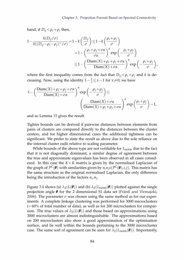
Chapter 3. Projection Pursuit Based on Spectral Connectivity
hand, if Dij<ρi+ρj then,
1−k(Dij/σ)
k((Dij−ρi−ρj)+/σ)=1−k
(Dij
σ
)≤1−k
(ρi+ρj
σ
)=1−
(ρi+ρj+σα
σα
)α
exp(−
ρi+ρj
σ
)≤1−
(Diam(X)+ρi+ρj+σα
Diam(X)+σα
)α
exp(−
ρi+ρj
σ
),
where the first inequality comes from the fact that Dij<ρi+ρj and k is de-creasing. Now, using the identity 1− 1
x≤x−1 for x 6=0, we have
1−(
Diam(X)+ρi+ρj+σα
Diam(X)+σα
)α
exp(−
ρi+ρj
σ
)≤(
Diam(X)+σα
Diam(X)+ρi+ρj+σα
)α
exp(
ρi+ρj
σ
)−1,
and so Lemma 15 gives the result.
Tighter bounds can be derived if pairwise distances between elements frompairs of clusters are compared directly to the distances between the clustercenters, and for higher dimensional cases the additional tightness can besignificant. We prefer to state the result as above due to the sole reliance onthe internal cluster radii relative to scaling parameter.
While bounds of the above type are not verifiable for Lnorm due to the factthat it is not diagonally dominant, a similar degree of agreement betweenthe true and approximate eigenvalues has been observed in all cases consid-ered. In this case the K×K matrix is given by the normalised Laplacian ofthe graph of PC(θθθ) with similarities given by ninjs(PC(θθθ), i, j). This matrix hasthe same structure as the original normalised Laplacian, the only differencebeing the introduction of the factors ni,nj.
Figure 3.4 shows (a) λ2(L(θθθ)) and (b) λ2(Lnorm(θθθ)) plotted against the singleprojection angle θθθ for the 2 dimensional S1 data set (Fränti and Virmajoki,2006). The parameter σ was chosen using the same method as for our exper-iments. A complete linkage clustering was performed for 3000 microclusters(=60% of total number of data), as well as for 200 microclusters for compar-ison. The true values of λ2(L(θθθ)) and those based on approximations using3000 microclusters are almost indistinguishable. The approximations basedon 200 microclusters also show a good approximation of the optimisationsurface, and lie well within the bounds pertaining to the 3000 microclustercase. The same sort of agreement can be seen for λ2(Lnorm(θθθ)). Importantly,
84
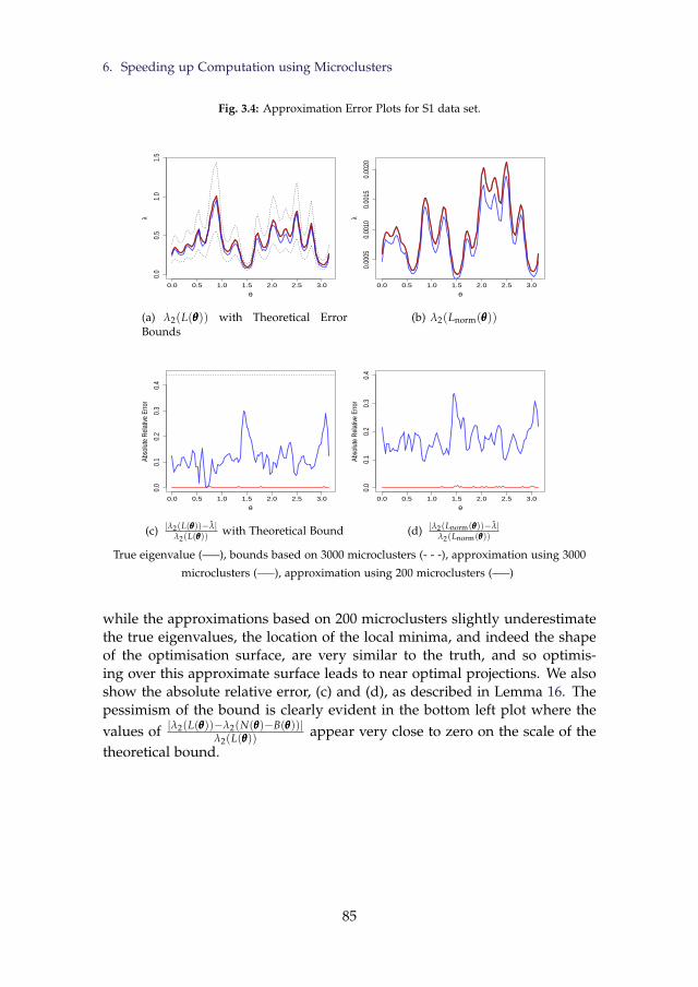
6. Speeding up Computation using Microclusters
Fig. 3.4: Approximation Error Plots for S1 data set.
0.0 0.5 1.0 1.5 2.0 2.5 3.0
0.0
0.5
1.0
1.5
θ
λ
(a) λ2(L(θθθ)) with Theoretical ErrorBounds
0.0 0.5 1.0 1.5 2.0 2.5 3.0
0.00
050.
0010
0.00
150.
0020
θ
λ
(b) λ2(Lnorm(θθθ))
0.0 0.5 1.0 1.5 2.0 2.5 3.0
0.0
0.1
0.2
0.3
0.4
θ
Abso
lute
Rel
ative
Erro
r
(c) |λ2(L(θθθ))−λ|λ2(L(θθθ)) with Theoretical Bound
0.0 0.5 1.0 1.5 2.0 2.5 3.0
0.0
0.1
0.2
0.3
0.4
θ
Abso
lute
Rel
ative
Erro
r
(d) |λ2(Lnorm(θθθ))−λ|λ2(Lnorm(θθθ))
True eigenvalue (—–), bounds based on 3000 microclusters (- - -), approximation using 3000
microclusters (—–), approximation using 200 microclusters (—–)
while the approximations based on 200 microclusters slightly underestimatethe true eigenvalues, the location of the local minima, and indeed the shapeof the optimisation surface, are very similar to the truth, and so optimis-ing over this approximate surface leads to near optimal projections. We alsoshow the absolute relative error, (c) and (d), as described in Lemma 16. Thepessimism of the bound is clearly evident in the bottom left plot where thevalues of |λ2(L(θθθ))−λ2(N(θθθ)−B(θθθ))|
λ2(L(θθθ)) appear very close to zero on the scale of thetheoretical bound.
85
Chapter 3. Projection Pursuit Based on Spectral Connectivity
7 Experimental Results
In this section we evaluate the proposed method on a large collection ofbenchmark datasets. We compare our approach with existing dimensionreduction methods for clustering, where the final clustering result is deter-mined using spectral clustering. In addition we consider solving our problemiteratively for a shrinking sequence of scaling parameters to find large mar-gin separators, relying on the theoretical results presented in Section 5. Wecompare these results with the iterative support vector regression approachof Zhang et al. (2009)3, a state-of-the-art maximum margin clustering algo-rithm.
We compare the different methods based on two popular evaluation met-rics for clustering, namely purity (Zhao and Karypis, 2004) and V-measure(Rosenberg and Hirschberg, 2007). Both metrics compare the label assign-ments made by a clustering algorithm with the true class labels of the data.They take values in [0,1] with larger values indicating a better agreementbetween the two label sets, and hence a superior clustering result. Purity isthe weighted average of the largest proportion of each cluster which can berepresented by a single class. V-measure is defined as the harmonic mean ofmeasures of completeness and homogeneity. Homogeneity is similar to pu-rity, in that it measures the extent to which each cluster may be representedby a single class, but is given by the weighted average of the entropy ofthe class distribution within each cluster. Completeness is symmetric to ho-mogeneity, and measures the entropy of the cluster distribution within eachclass. V-measure therefore also captures the extent to which classes are splitbetween clusters.
We will use the following notation throughout this section:
• SCP2 and SCnP2 refer to the proposed projection pursuits for minimis-ing λ2(L(θθθ)) and λ2(Lnorm(θθθ)) respectively.
• LMSC refers to the proposed approach of finding large margin separa-tors, based on repeatedly minimising λ2(L(θθθ)) for a shrinking sequenceof scaling parameters.
• Subscripts “o" and “c" indicate whether we use an orthogonal projection(ω>0) or a correlated one (ω<0), respectively.
• SC and SCn refer to spectral clustering based on the eigen-decompositionsof L and Lnorm respectively.
• Subscripts “PCA" and “ICA" indicate principal and independent com-ponent analysis projections respectively. For example, SCnPCA refers to
3We are grateful to Dr. Kai Zhang for supplying us with code to implement this method.
86
7. Experimental Results
spectral clustering using the normalised Laplacian applied to the dataprojected into a principal component oriented subspace.
• DRSC abbreviates dimensionality reduction for spectral clustering, pro-posed by Niu et al. (2011). This existing approach applies only to thenormalised Laplacian.
• iSVRL and iSVRG denote the iterative support vector regression ap-proach for maximum margin clustering (Zhang et al., 2009), using thelinear and Gaussian kernels respectively.
7.1 Details of Implementation
To extend our approach to datasets containing multiple clusters, we sim-ply recursively partition (subsets of) the dataset until the desired number ofclusters is obtained. We prefer this approach to the alternative of directlyseeking a projection which yields a full K way partition of the dataset, i.e.,by minimising the sum of the first K eigenvalues of the Laplacians, as it isnot always clear that all the clusters present in the data can be exposed us-ing a single projection of fixed dimension. At each iteration in this recursivebi-partitioning we split the largest remaining cluster.
The scaling parameter and initialisation are set for each bi-partition, givenvalues determined by the subset of the data being partitioned. For thefixed scaling parameter approaches, SCP2 and SCnP2, we set σ=
√lλdN−1/5,
where l is the dimension of the projection, N is the size of the (subset of the)data and λd is the largest eigenvalue of the covariance matrix. The value√
λd captures the scale of the data, while√
l accounts for the fact that dis-tances scale roughly with the square root of the dimension. The denominatorterm, N−1/5, is borrowed from kernel density methods and we have foundit to work reasonably well for our applications as well. For the large mar-gin approach, LMSC, σ is initialised at
√lλdN−1/5 and decreased by a factor
of two with each minimisation of λ2(L(θθθ)), until convergence of the projec-tion matrix. The initialisation of V(θθθ) is via the first l principal components.For the orthogonal projections we use a two dimensional projection, as thisis the lowest dimensional space which can expose non-linear separation be-tween clusters. For the correlated projections we provide a three dimensionalinitialisation, and it was found that in most cases a high quality univariateprojection could be determined from this.
For the LMSC approach, because the values within the Laplacian matrixapproach zero, the optimisation becomes less robust, and we found that thecorrelated approach did not always lead to large margin separation. Webelieve this is as a result of the term controlling the correlation becomingtoo dominant relative to the decreasing eigenvalue unless very careful tuning
87
Chapter 3. Projection Pursuit Based on Spectral Connectivity
of ω is performed. We therefore consider a univariate projection instead ofthe multivariate correlated approach in this case.
Recall that the parameter β controls the size of the constraint set ∆. It isclear that smaller values of β will tend to lead to more balanced partitions, buta precise interpretation of the resulting cluster sizes is unavailable. At bestbounds on the cluster sizes can be computed using Chebyshev’s inequality.Rather than relying on these bounds, which may be loose and difficult tointerpret in multivariate projections, we recommend applying the proposedmethod for a range of values of β and selecting the solution corresponding tothe largest value of β which induces a specified balance in the partition. Wedefine this balance to be satisfied if the smallest cluster size is at least half theaverage, i.e., N/2K. In this way the effect of the constraint is limited whilestill producing the desired result. We initialise with a large value of β anddecrease by 0.5 until the balance is met. If this balance is not met for β=0.5,then the corresponding “unbalanced" result is returned anyway.
The parameter δ is set to min0.01,σ2 and α to 0.1. We have found thesetwo parameters not to significantly influence the performance of the method.It is important to note, however, that that parameter α controls the shape ofthe similarity function, and as a result there is an interplay between this valueand the value of σ. For substantially larger values of α we expect a smallervalue of σ to be more appropriate.
For competing approaches based on spectral clustering we do the follow-ing. Whenever the number of data exceeds 1000 we use the approximationmethod of Yan et al. (2009). Following Niu et al. (2011), we set the reduceddimension to K−1, where K is the number of clusters. We compute cluster-ing results for all values of σ in 0.1,0.2,0.5,1,2,5,10,20,50, 100,200 as wellas for the local scaling approach of Zelnik-Manor and Perona (2004), and re-port the highest performance in each case. For DRSC we also considered theparameter setting used for our method, and to implement the local scalingsof Zelnik-Manor and Perona (2004) these were recomputed with each itera-tion in the corresponding projected subspace. We also provided DRSC witha warm start via PCA as this improved performance over a random initial-isation, and offers a more fair comparison. Because of this extensive searchover scaling parameters we expect competing methods to achieve very highperformance whenever the corresponding dimension reduction is capable ofexposing the clusters in the data well.
For the iSVR maximum margin clustering method, we set the balancingparameter equal to 0.3 as suggested by Zhang et al. (2009) when the clustersizes are not balanced. We argue that the balance of the clusters will not beknown in practice, and the unbalanced setting led to superior performancecompared with the balanced setting in the examples considered. The iSVRapproach also generates only a bi-partition, and to generate multiple clusterswe apply the same recursive approach as in our method.
88
7. Experimental Results
7.2 Clustering Results
The following benchmark datasets were used for comparison:
• Optical recognition of handwritten digits (Opt. Digits).4 5620 8×8 com-pressed images of handwritten digits in 0,...,9, resulting in 64 dimen-sions with 10 classes.
• Pen based recognition of handwritten digits (Pen Digits).2 10992 ob-servations, each corresponding to a stylus trajectory (x,y coordinates)from a handwritten digit in 0,...,9, i.e., 10 classes. The trajectories aresampled at 8 time points, resulting in 16 dimensions.
• Satellite.2 6435 multispectral values from 3×3 pixel squares from satel-lite images, which results in 36 dimensions. There are 6 classes corre-sponding to different land types.
• Breast cancer Wisconsin (Br. Cancer).2 699 observations with 9 at-tributes relating to tumour masses. There are 2 classes correspondingto benign and malignant masses.
• Congressional votes (Voters).2 435 sets of 16 binary decisions on UScongressional ballots. The 2 classes correspond to political party mem-bership.
• Dermatology.2 366 observations corresponding to dermatology patients,each containing 34 dimensions derived from clinical and histopatho-logical features. There are 6 classes corresponding to different skindiseases.
• Yeast cell cycle analysis (Yeast).5 698 yeast genes across 72 conditions(dimensions). There are 5 classes corresponding to different genotypes.
• Synthetic control chart (Chart).2 600 simulated time series of length 60displaying one of 6 fundamental characteristics, leading to 6 classes.
• Multiple feature digits (M.F. Digits).2 2000 handwritted digits in 0,...,9taken from Dutch utility maps. Following Niu et al. (2011) we use onlythe 216 profile correlation features.
• Statlog image segmentation (Image Seg.).2 2310 observations containing19 features derived from 3×3 pixel squares from 7 outdoor images.Each image constitutes a class.
4https://archive.ics.uci.edu/ml/datasets.html5http://genome-www.stanford.edu/cellcycle/
89
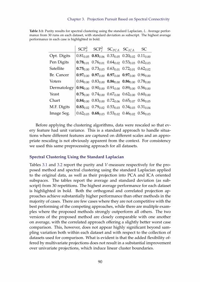
Chapter 3. Projection Pursuit Based on Spectral Connectivity
Table 3.1: Purity results for spectral clustering using the standard Laplacian, L. Average perfor-mance from 30 runs on each dataset, with standard deviation as subscript. The highest averageperformance in each case is highlighted in bold.
SCP2o SCP2
c SCPCA SCICA SC
Opt. Digits 0.810.05 0.830.06 0.330.05 0.200.02 0.110.00
Pen Digits 0.780.01 0.760.01 0.640.02 0.530.03 0.620.03
Satellite 0.750.00 0.730.03 0.630.01 0.720.01 0.620.02
Br. Cancer 0.970.00 0.970.00 0.970.00 0.970.00 0.960.00
Voters 0.840.00 0.830.00 0.860.00 0.860.00 0.780.00
Dermatology 0.940.00 0.900.00 0.910.00 0.890.00 0.560.00
Yeast 0.750.00 0.740.00 0.670.00 0.620.00 0.600.00
Chart 0.840.00 0.830.00 0.720.06 0.650.07 0.560.05
M.F. Digits 0.830.02 0.790.02 0.530.03 0.340.03 0.310.04
Image Seg. 0.620.03 0.680.03 0.530.02 0.460.02 0.560.03
Before applying the clustering algorithms, data were rescaled so that ev-ery feature had unit variance. This is a standard approach to handle situa-tions where different features are captured on different scales and an appro-priate rescaling is not obviously apparent from the context. For consistencywe used this same preprocessing approach for all datasets.
Spectral Clustering Using the Standard Laplacian
Tables 3.1 and 3.2 report the purity and V-measure respectively for the pro-posed method and spectral clustering using the standard Laplacian appliedto the original data, as well as their projection into PCA and ICA orientedsubspaces. The tables report the average and standard deviation (as sub-script) from 30 repetitions. The highest average performance for each datasetis highlighted in bold. Both the orthogonal and correlated projection ap-proaches achieve substantially higher performance than other methods in themajority of cases. There are few cases where they are not competitive with thebest performing of the competing approaches, while there are mulitple exam-ples where the proposed methods strongly outperform all others. The twoversions of the proposed method are closely comparable with one anotheron average, with the correlated approach offering a slightly better worst casecomparison. This, however, does not appear highly significant beyond sam-pling variation both within each dataset and with respect to the collection ofdatasets used for comparison. What is evident is that the added flexibility of-fered by multivariate projections does not result in a substantial improvementover univariate projections, which induce linear cluster boundaries.
90
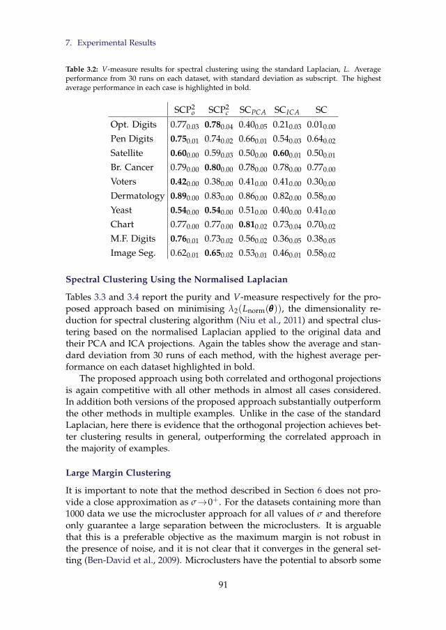
7. Experimental Results
Table 3.2: V-measure results for spectral clustering using the standard Laplacian, L. Averageperformance from 30 runs on each dataset, with standard deviation as subscript. The highestaverage performance in each case is highlighted in bold.
SCP2o SCP2
c SCPCA SCICA SC
Opt. Digits 0.770.03 0.780.04 0.400.05 0.210.03 0.010.00
Pen Digits 0.750.01 0.740.02 0.660.01 0.540.03 0.640.02
Satellite 0.600.00 0.590.03 0.500.00 0.600.01 0.500.01
Br. Cancer 0.790.00 0.800.00 0.780.00 0.780.00 0.770.00
Voters 0.420.00 0.380.00 0.410.00 0.410.00 0.300.00
Dermatology 0.890.00 0.830.00 0.860.00 0.820.00 0.580.00
Yeast 0.540.00 0.540.00 0.510.00 0.400.00 0.410.00
Chart 0.770.00 0.770.00 0.810.02 0.730.04 0.700.02
M.F. Digits 0.760.01 0.730.02 0.560.02 0.360.05 0.380.05
Image Seg. 0.620.01 0.650.02 0.530.01 0.460.01 0.580.02
Spectral Clustering Using the Normalised Laplacian
Tables 3.3 and 3.4 report the purity and V-measure respectively for the pro-posed approach based on minimising λ2(Lnorm(θθθ)), the dimensionality re-duction for spectral clustering algorithm (Niu et al., 2011) and spectral clus-tering based on the normalised Laplacian applied to the original data andtheir PCA and ICA projections. Again the tables show the average and stan-dard deviation from 30 runs of each method, with the highest average per-formance on each dataset highlighted in bold.
The proposed approach using both correlated and orthogonal projectionsis again competitive with all other methods in almost all cases considered.In addition both versions of the proposed approach substantially outperformthe other methods in multiple examples. Unlike in the case of the standardLaplacian, here there is evidence that the orthogonal projection achieves bet-ter clustering results in general, outperforming the correlated approach inthe majority of examples.
Large Margin Clustering
It is important to note that the method described in Section 6 does not pro-vide a close approximation as σ→0+. For the datasets containing more than1000 data we use the microcluster approach for all values of σ and thereforeonly guarantee a large separation between the microclusters. It is arguablethat this is a preferable objective as the maximum margin is not robust inthe presence of noise, and it is not clear that it converges in the general set-ting (Ben-David et al., 2009). Microclusters have the potential to absorb some
91

Chapter 3. Projection Pursuit Based on Spectral Connectivity
Table 3.3: Purity results for spectral clustering using the normalised Laplacian, Lnorm. Averageperformance from 30 runs on each dataset, with standard deviation as subscript. The highestaverage performance in each case is highlighted in bold.
SCnP2o SCnP2
c DRSC SCnPCA SCnICA SCn
Opt. Digits 0.810.05 0.740.06 0.800.03 0.660.03 0.640.01 0.660.02
Pen Digits 0.780.00 0.740.02 0.690.04 0.760.03 0.740.01 0.770.04
Satellite 0.750.00 0.740.03 0.730.01 0.760.01 0.730.02 0.740.01
Br. Cancer 0.970.00 0.970.00 0.960.00 0.970.00 0.970.00 0.970.00
Voters 0.850.00 0.840.00 0.860.00 0.860.00 0.860.00 0.850.00
Dermatology 0.860.00 0.910.00 0.870.00 0.920.02 0.910.00 0.950.00
Yeast 0.760.00 0.700.00 0.620.00 0.710.00 0.690.01 0.600.00
Chart 0.870.00 0.850.00 0.750.00 0.710.06 0.800.07 0.750.00
M.F. Digits 0.840.01 0.790.01 0.770.03 0.770.03 0.790.01 0.770.02
Image Seg. 0.660.01 0.700.01 0.650.04 0.610.03 0.550.02 0.620.02
Table 3.4: V-measure results for spectral clustering using the normalised Laplacian, Lnorm. Av-erage performance from 30 runs on each dataset, with standard deviation as subscript. Thehighest average performance in each case is highlighted in bold.
SCnP2o SCnP2
c DRSC SCnPCA SCnICA SCn
Opt. Digits 0.770.03 0.720.04 0.750.02 0.620.02 0.600.01 0.620.01
Pen Digits 0.760.00 0.740.01 0.660.02 0.720.01 0.680.01 0.730.02
Satellite 0.610.01 0.600.03 0.570.01 0.620.01 0.600.05 0.600.01
Br. Cancer 0.790.00 0.810.00 0.760.00 0.810.00 0.810.00 0.790.00
Voters 0.420.00 0.410.00 0.420.00 0.410.00 0.410.00 0.420.00
Dermatology 0.850.00 0.860.00 0.800.00 0.860.02 0.830.00 0.910.00
Yeast 0.570.00 0.450.00 0.410.00 0.540.00 0.530.00 0.450.00
Chart 0.810.00 0.800.00 0.750.00 0.810.02 0.800.05 0.730.00
M.F. Digits 0.760.01 0.740.02 0.690.02 0.710.02 0.750.01 0.700.02
Image Seg. 0.650.01 0.680.01 0.620.04 0.600.02 0.460.02 0.600.02
92

7. Experimental Results
Table 3.5: Purity results for large margin clustering. Average performance from 30 runs on eachdataset, with standard deviation as subscript. The highest average performance in each case ishighlighted in bold.
LMSCo LMSC iSVRL iSVRG
Opt. Digits 0.740.05 0.690.05 0.760.00 0.610.01
Pen Digits 0.800.02 0.710.04 0.780.00 0.780.00
Satellite 0.750.01 0.720.03 0.680.00 0.680.00
Br. Cancer 0.960.00 0.970.00 0.900.00 0.950.00
Voters 0.840.00 0.840.00 0.810.00 0.840.00
Dermatology 0.860.00 0.860.00 0.800.00 0.800.00
Yeast 0.750.00 0.750.00 0.750.00 0.700.00
Chart 0.890.00 0.830.00 0.720.00 0.720.00
M.F. Digits 0.820.05 0.740.04 0.670.00 0.600.01
Image Seg. 0.600.04 0.650.03 0.640.00 0.660.01
of the noise in the data, and in the event that they are of roughly equaldensity, maximising the margin over the microcluster centers has a similareffect to that of minimising the empirical density in a neighbourhood of thecorresponding hyperplane separator. This is reminiscent of the soft-marginapproach which does enjoy strong convergence properties (Ben-David et al.,2009). In addition, since the optimisation is reinitialised for each value of σ,we are able to recompute the microclusters by performing the coarse clus-tering on the projected data with each iteration. This tends to lead to themargins in the microclusters being more closely related to the margins in thefull dataset along the optimal projections.
Tables 3.5 and 3.6 report the average and standard deviation of the pro-posed LMSC as well as the iterative support vector regression approach (Zhanget al., 2009) using both a linear and Gaussian kernel for comparison. Bothversions of LMSC, using an orthogonal two dimensional and a one dimen-sional projection, outperform both versions of the iterative support vectorregression in the majority of cases, with substantially higher performance inmultiple examples. There is strong evidence that the two dimensional LMSCoobtains better quality clustering results than the one dimensional alternative,showing sunstantially higher performance in the vast majority of cases con-sidered.
7.3 Summarising Clustering Performance
Thus far we have compared different approaches for standard and normalisedspectral clustering and for large margin clustering separately. These separate
93
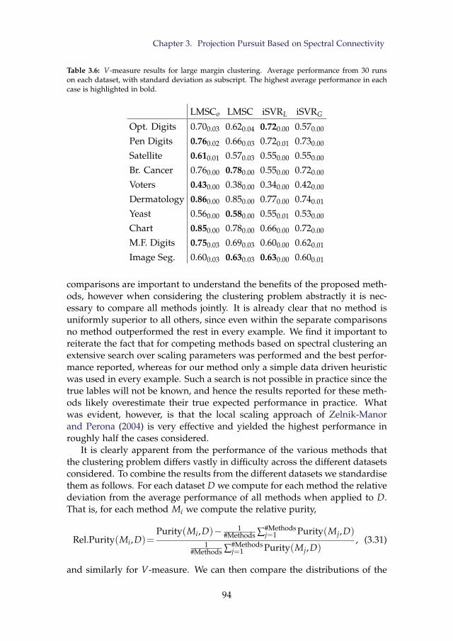
Chapter 3. Projection Pursuit Based on Spectral Connectivity
Table 3.6: V-measure results for large margin clustering. Average performance from 30 runson each dataset, with standard deviation as subscript. The highest average performance in eachcase is highlighted in bold.
LMSCo LMSC iSVRL iSVRG
Opt. Digits 0.700.03 0.620.04 0.720.00 0.570.00
Pen Digits 0.760.02 0.660.03 0.720.01 0.730.00
Satellite 0.610.01 0.570.03 0.550.00 0.550.00
Br. Cancer 0.760.00 0.780.00 0.550.00 0.720.00
Voters 0.430.00 0.380.00 0.340.00 0.420.00
Dermatology 0.860.00 0.850.00 0.770.00 0.740.01
Yeast 0.560.00 0.580.00 0.550.01 0.530.00
Chart 0.850.00 0.780.00 0.660.00 0.720.00
M.F. Digits 0.750.03 0.690.03 0.600.00 0.620.01
Image Seg. 0.600.03 0.630.03 0.630.00 0.600.01
comparisons are important to understand the benefits of the proposed meth-ods, however when considering the clustering problem abstractly it is nec-essary to compare all methods jointly. It is already clear that no method isuniformly superior to all others, since even within the separate comparisonsno method outperformed the rest in every example. We find it important toreiterate the fact that for competing methods based on spectral clustering anextensive search over scaling parameters was performed and the best perfor-mance reported, whereas for our method only a simple data driven heuristicwas used in every example. Such a search is not possible in practice since thetrue lables will not be known, and hence the results reported for these meth-ods likely overestimate their true expected performance in practice. Whatwas evident, however, is that the local scaling approach of Zelnik-Manorand Perona (2004) is very effective and yielded the highest performance inroughly half the cases considered.
It is clearly apparent from the performance of the various methods thatthe clustering problem differs vastly in difficulty across the different datasetsconsidered. To combine the results from the different datasets we standardisethem as follows. For each dataset D we compute for each method the relativedeviation from the average performance of all methods when applied to D.That is, for each method Mi we compute the relative purity,
Rel.Purity(Mi,D)=Purity(Mi,D)− 1
#Methods ∑#Methodsj=1 Purity(Mj,D)
1#Methods ∑#Methods
j=1 Purity(Mj,D), (3.31)
and similarly for V-measure. We can then compare the distributions of the
94
7. Experimental Results
relative performance measures from all datasets and for all methods. It isclear from Table 3.1 that the competing methods SC, SCPCA and SCICA are notcompetitive with other methods in general, due to their vastly inferior per-formance on multiple datasets. Moreover, their performance is sufficientlylow to obscure the comparisons between others. These three methods aretherefore omitted from this comparison. Figures 3.5 and 3.6 show boxplotsof the relative performance measures for all other methods. The additionalred dots indicate the mean relative performance measures for each method,and methods are ordered in decreasing order of their means. In the caseof purity, all of the proposed methods outperform every method used forcomparison, and except for the univariate large margin method, LMSC, thedifference between the proposed methods and the methods used for compar-ison is substantial. In the case of V-measure, the same is true except thatin this case LMSC is outperformed on average by spectral clustering usingthe normalised Laplacian applied to the PCA projected data. Notice thatthe most relevant comparison for LMSC is with iSVRL because of their sim-ilar objectives. In terms of both purity and V-measure, LMSC significantlyoutperformed the existing large margin clustering method.
Among the methods used for comparison, it is evident that spectral clus-tering is capable of outperforming existing large margin clustering methods,provided an appropriate scaling parameter can be determined. Of those spec-tral clustering variants, PCA projections showed the best overall performance.While the DRSC method (Niu et al., 2011) in some cases showed a substantialimprovement over the simpler dimension reduction of PCA, it did not yieldconsistently higher performance on the datasets considered.
Overall it is apparent that the proposed approach for projection pursuitbased on spectral connectivity is highly competitive with existing dimensionreduction methods. Moreover, a simple data driven heuristic allowed us toselect the important scaling parameter automotically without tuning it foreach dataset, as is recommended for the DRSC method (Niu et al., 2011).Among the variants of the proposed approaches, it is evident that while theflexibility of the multivariate projections offered higher performance on aver-age than the corresponding univariate projections, it is only in the case of thelarge margin separation methods that this improvement is significant beyondthe variation from the collection of datasets used for comparison.
7.4 Sensitivity Analysis
In this subsection we investigate the sensitivity of the proposed approach tothe setting of the important scaling parameter, σ. In addition we consider theeffect on performance of the number of microclusters used in approximat-ing the optimisation surface. For the former we consider the breast cancer,voters, dermatology, yeast and chart datasets as these exhibited very low vari-
95
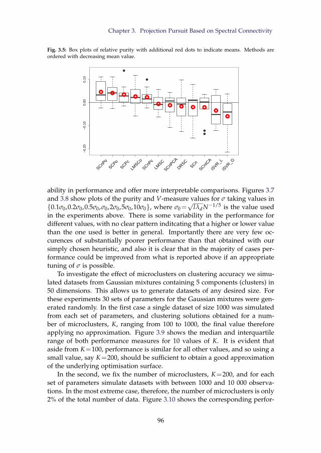
Chapter 3. Projection Pursuit Based on Spectral Connectivity
Fig. 3.5: Box plots of relative purity with additional red dots to indicate means. Methods areordered with decreasing mean value.
−0.
20−
0.10
0.00
0.10
SCnPo
SCPoSCPc
LMSCo
SCnPc
LMSC
SCnPCA
DRSCSCn
SCnICA
iSVR_L
iSVR_G
ability in performance and offer more interpretable comparisons. Figures 3.7and 3.8 show plots of the purity and V-measure values for σ taking values in0.1σ0,0.2σ0,0.5σ0,σ0,2σ0,5σ0,10σ0, where σ0=
√lλdN−1/5 is the value used
in the experiments above. There is some variability in the performance fordifferent values, with no clear pattern inditcating that a higher or lower valuethan the one used is better in general. Importantly there are very few oc-curences of substantially poorer performance than that obtained with oursimply chosen heuristic, and also it is clear that in the majority of cases per-formance could be improved from what is reported above if an appropriatetuning of σ is possible.
To investigate the effect of microclusters on clustering accuracy we simu-lated datasets from Gaussian mixtures containing 5 components (clusters) in50 dimensions. This allows us to generate datasets of any desired size. Forthese experiments 30 sets of parameters for the Gaussian mixtures were gen-erated randomly. In the first case a single dataset of size 1000 was simulatedfrom each set of parameters, and clustering solutions obtained for a num-ber of microclusters, K, ranging from 100 to 1000, the final value thereforeapplying no approximation. Figure 3.9 shows the median and interquartilerange of both performance measures for 10 values of K. It is evident thataside from K=100, performance is similar for all other values, and so using asmall value, say K=200, should be sufficient to obtain a good approximationof the underlying optimisation surface.
In the second, we fix the number of microclusters, K=200, and for eachset of parameters simulate datasets with between 1000 and 10 000 observa-tions. In the most extreme case, therefore, the number of microclusters is only2% of the total number of data. Figure 3.10 shows the corresponding perfor-
96
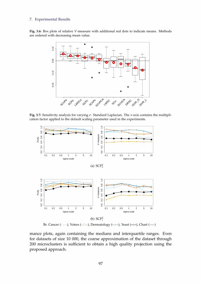
7. Experimental Results
Fig. 3.6: Box plots of relative V-measure with additional red dots to indicate means. Methodsare ordered with decreasing mean value.
−0.
20−
0.10
0.00
0.10
SCnPo
SCPo
LMSCo
SCPc
SCnPc
SCnPCA
LMSC
SCn
SCnICA
DRSC
iSVR_G
iSVR_L
Fig. 3.7: Sensitivity analysis for varying σ. Standard Laplacian. The x-axis contains the multipli-cation factor applied to the default scaling parameter used in the experiments.
0.0
0.2
0.4
0.6
0.8
1.0
sigma scale
Pur
ity
0.1 0.2 0.5 1 2 5 10
0.0
0.2
0.4
0.6
0.8
1.0
sigma scale
V−
mea
sure
0.1 0.2 0.5 1 2 5 10
(a) SCP2o
0.0
0.2
0.4
0.6
0.8
1.0
sigma scale
Pur
ity
0.1 0.2 0.5 1 2 5 10
0.0
0.2
0.4
0.6
0.8
1.0
sigma scale
V−
mea
sure
0.1 0.2 0.5 1 2 5 10
(b) SCP2c
Br. Cancer (–+–), Voters (–4–), Dermatology (–×–), Yeast (––), Chart (––)
mance plots, again containing the medians and interquartile ranges. Evenfor datasets of size 10 000, the coarse approximation of the dataset through200 microclusters is sufficient to obtain a high quality projection using theproposed approach.
97
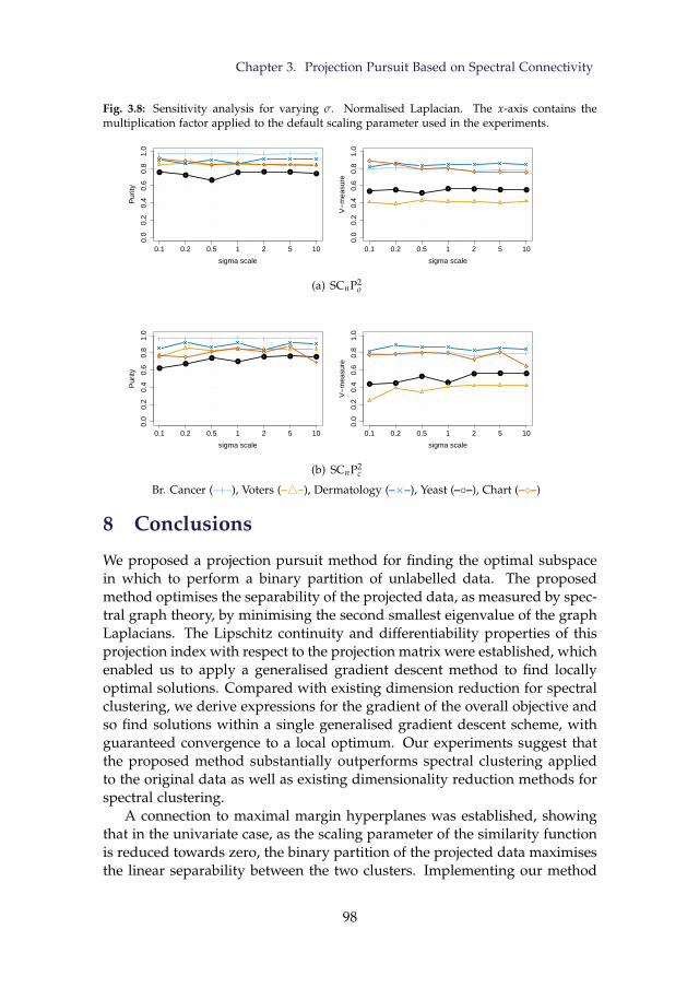
Chapter 3. Projection Pursuit Based on Spectral Connectivity
Fig. 3.8: Sensitivity analysis for varying σ. Normalised Laplacian. The x-axis contains themultiplication factor applied to the default scaling parameter used in the experiments.
0.0
0.2
0.4
0.6
0.8
1.0
sigma scale
Pur
ity
0.1 0.2 0.5 1 2 5 10
0.0
0.2
0.4
0.6
0.8
1.0
sigma scale
V−
mea
sure
0.1 0.2 0.5 1 2 5 10
(a) SCnP2o
0.0
0.2
0.4
0.6
0.8
1.0
sigma scale
Pur
ity
0.1 0.2 0.5 1 2 5 10
0.0
0.2
0.4
0.6
0.8
1.0
sigma scale
V−
mea
sure
0.1 0.2 0.5 1 2 5 10
(b) SCnP2c
Br. Cancer (–+–), Voters (–4–), Dermatology (–×–), Yeast (––), Chart (––)
8 Conclusions
We proposed a projection pursuit method for finding the optimal subspacein which to perform a binary partition of unlabelled data. The proposedmethod optimises the separability of the projected data, as measured by spec-tral graph theory, by minimising the second smallest eigenvalue of the graphLaplacians. The Lipschitz continuity and differentiability properties of thisprojection index with respect to the projection matrix were established, whichenabled us to apply a generalised gradient descent method to find locallyoptimal solutions. Compared with existing dimension reduction for spectralclustering, we derive expressions for the gradient of the overall objective andso find solutions within a single generalised gradient descent scheme, withguaranteed convergence to a local optimum. Our experiments suggest thatthe proposed method substantially outperforms spectral clustering appliedto the original data as well as existing dimensionality reduction methods forspectral clustering.
A connection to maximal margin hyperplanes was established, showingthat in the univariate case, as the scaling parameter of the similarity functionis reduced towards zero, the binary partition of the projected data maximisesthe linear separability between the two clusters. Implementing our method
98
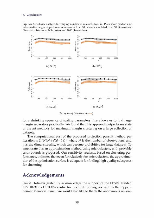
8. Conclusions
Fig. 3.9: Sensitivity analysis for varying number of microclusters, K. Plots show median andinterquartile ranges of performance measures from 30 datasets simulated from 50 dimensionalGaussian mixtures with 5 clusters and 1000 observations.
200 400 600 800 1000
0.0
0.2
0.4
0.6
0.8
1.0
K
Per
form
ance
(a) SCP2o
200 400 600 800 1000
0.0
0.2
0.4
0.6
0.8
1.0
K
Per
form
ance
(b) SCP2c
200 400 600 800 1000
0.0
0.2
0.4
0.6
0.8
1.0
K
Per
form
ance
(c) SCnP2o
200 400 600 800 1000
0.0
0.2
0.4
0.6
0.8
1.0
K
Per
form
ance
(d) SCnP2c
Purity (––), V-measure (––)
for a shrinking sequence of scaling parameters thus allows us to find largemargin separators practically. We found that this approach outperforms stateof the art methods for maximum margin clustering on a large collection ofdatasets.
The computational cost of the proposed projection pursuit method periteration is O(N(N+d(d−1))), where N is the number of observations, andd is the dimensionality, which can become prohibitive for large datasets. Toameliorate this an approximation method using microclusters, with provableerror bounds is proposed. Our sensitivity analysis, based on clustering per-formance, indicates that even for relatively few microclusters, the approxima-tion of the optimisation surface is adequate for finding high quality subspacesfor clustering.
Acknowledgements
David Hofmeyr gratefully acknowledges the support of the EPSRC fundedEP/H023151/1 STOR-i centre for doctoral training, as well as the Oppen-heimer Memorial Trust. We would also like to thank the anonymous review-
99
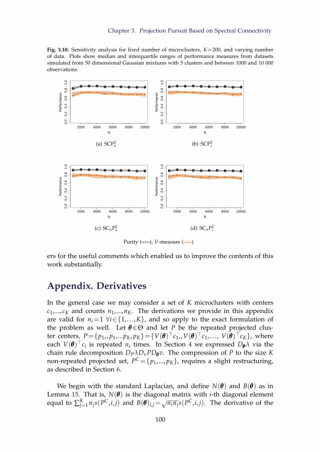
Chapter 3. Projection Pursuit Based on Spectral Connectivity
Fig. 3.10: Sensitivity analysis for fixed number of microclusters, K=200, and varying numberof data. Plots show median and interquartile ranges of performance measures from datasetssimulated from 50 dimensional Gaussian mixtures with 5 clusters and between 1000 and 10 000observations.
2000 4000 6000 8000 10000
0.0
0.2
0.4
0.6
0.8
1.0
N
Per
form
ance
(a) SCP2o
2000 4000 6000 8000 10000
0.0
0.2
0.4
0.6
0.8
1.0
N
Per
form
ance
(b) SCP2c
2000 4000 6000 8000 10000
0.0
0.2
0.4
0.6
0.8
1.0
N
Per
form
ance
(c) SCnP2o
2000 4000 6000 8000 10000
0.0
0.2
0.4
0.6
0.8
1.0
N
Per
form
ance
(d) SCnP2c
Purity (––), V-measure (––)
ers for the useful comments which enabled us to improve the contents of thiswork substantially.
Appendix. Derivatives
In the general case we may consider a set of K microclusters with centersc1, ...,cK and counts n1, ...,nK. The derivations we provide in this appendixare valid for ni=1 ∀i∈1, . . . ,K, and so apply to the exact formulation ofthe problem as well. Let θθθ∈Θ and let P be the repeated projected clus-ter centers, P=p1, , p1, ...pK, pK=V(θθθ)>c1, ,V(θθθ)>c1, . . . , V(θθθ)>cK, whereeach V(θθθ)>ci is repeated ni times. In Section 4 we expressed Dθθθλ via thechain rule decomposition DPλDvPDθθθv. The compression of P to the size Knon-repeated projected set, PC=p1, ..., pK, requires a slight restructuring,as described in Section 6.
We begin with the standard Laplacian, and define N(θθθ) and B(θθθ) as inLemma 15. That is, N(θθθ) is the diagonal matrix with i-th diagonal elementequal to ∑K
j=1 njs(PC, i, j) and B(θθθ)i,j=√ninjs(PC, i, j). The derivative of the
100
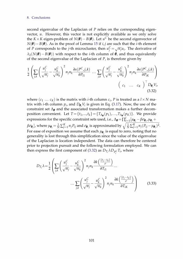
8. Conclusions
second eigenvalue of the Laplacian of P relies on the corresponding eigen-vector, u. However, this vector is not explicitly available as we only solvethe K×K eigen-problem of N(θθθ)−B(θθθ). Let uC be the second eigenvector ofN(θθθ)−B(θθθ). As in the proof of Lemma 15 if i, j are such that the i-th elementof P corresponds to the j-th microcluster, then uC
j =√njui. The derivative of
λ2(N(θθθ)−B(θθθ)) with respect to the i-th column of θθθ, and thus equivalentlyof the second eigenvalue of the Laplacian of P, is therefore given by
12
∑j,k
(uC
j√nj−
uCk√nk
)2
njnk∂s(PC, j,k)
∂Pi1. . . ∑
j,k
(uC
j√nj−
uCk√nk
)2
njnk∂s(PC, j,k)
∂PiK
(
c1 . . . cK
)>Dθθθi
Vi,
(3.32)
where (c1 . . . cK) is the matrix with i-th column ci, P is treated as a l×N ma-trix with i-th column pi, and Dθθθi
Vi is given in Eq. (3.17). Now, the use of theconstraint set ∆θθθ and the associated transformation makes a further decom-position convenient. Let T=t1, ...,tk=T∆θθθ
(p1), . . . ,T∆θθθ(pK). We provide
expressions for the specific constraint sets used, i.e., ∆θθθ =∏li=1[µθθθi
−βσθθθi,µθθθi
+
βσθθθi], where µθθθi
= 1N ∑K
j=1 njPij and σθθθiis approximated by
√1N ∑K
j=1 nj(Pij−µθθθi)2.
For ease of exposition we assume that each µθθθiis equal to zero, noting that no
generality is lost through this simplification since the value of the eigenvalueof the Laplacian is location independent. The data can therefore be centeredprior to projection pursuit and the following formulation employed. We canthen express the first component of (3.32) as DTi λDPC
iTi, where
DTi λ=12
∑j,k
(uC
j√nj−
uCk√nk
)2
njnk
∂k( ‖tj−tk‖
σ
)∂Ti1
...
... ∑j,k
(uC
j√nj−
uCk√nk
)2
njnk
∂k( ‖tj−tk‖
σ
)∂TiK
(3.33)
101
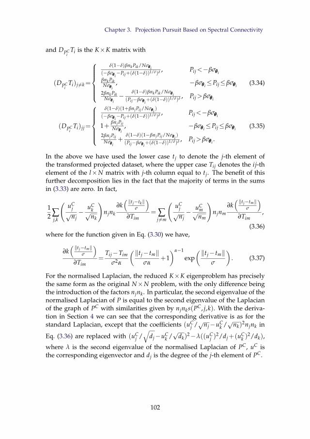
Chapter 3. Projection Pursuit Based on Spectral Connectivity
and DPCi
Ti is the K×K matrix with
(DPCi
Ti)j 6=k=
δ(1−δ)βnk Pik/Nσθθθi
(−βσθθθi−Pij+(δ(1−δ))1/δ)δ , Pij<−βσθθθi
βnk PikNσθθθi
, −βσθθθi≤Pij≤βσθθθi
2βnk PikNσθθθi
−δ(1−δ)βnk Pik/Nσθθθi
(Pij−βσθθθi+(δ(1−δ))1/δ)δ , Pij>βσθθθi
(3.34)
(DPCi
Ti)jj=
δ(1−δ)(1+βnjPij/Nσθθθi
)
(−βσθθθi−Pij+(δ(1−δ))1/δ)δ , Pij<−βσθθθi
1+βnjPijNσθθθi
, −βσθθθi≤Pij≤βσθθθi
2βnjPijNσθθθi
+δ(1−δ)(1−βnjPij/Nσθθθi
)
(Pij−βσθθθi+(δ(1−δ))1/δ)δ , Pij>βσθθθi
.
(3.35)
In the above we have used the lower case tj to denote the j-th element ofthe transformed projected dataset, where the upper case Tij denotes the ij-thelement of the l×N matrix with j-th column equal to tj. The benefit of thisfurther decomposition lies in the fact that the majority of terms in the sumsin (3.33) are zero. In fact,
12 ∑
j,k
(uC
j√nj−
uCk√nk
)njnk
∂k( ‖tj−tk‖
σ
)∂Tim
= ∑j 6=m
(uC
j√nj− uC
m√nm
)njnm
∂k( ‖tj−tm‖
σ
)∂Tim
,
(3.36)where for the function given in Eq. (3.30) we have,
∂k( ‖tj−tm‖
σ
)∂Tim
=Tij−Tim
σ2α
(‖tj− tm‖σα
+1)α−1
exp(‖tj− tm‖
σ
). (3.37)
For the normalised Laplacian, the reduced K×K eigenproblem has preciselythe same form as the original N×N problem, with the only difference beingthe introduction of the factors njnk. In particular, the second eigenvalue of thenormalised Laplacian of P is equal to the second eigenvalue of the Laplacianof the graph of PC with similarities given by njnks(PC, j,k). With the deriva-tion in Section 4 we can see that the corresponding derivative is as for thestandard Laplacian, except that the coefficients (uC
j /√nj−uCk /√
nk)2njnk in
Eq. (3.36) are replaced with (uCj /√
dj−uCk /√
dk)2−λ((uC
j )2/dj+(uC
k )2/dk),
where λ is the second eigenvalue of the normalised Laplacian of PC, uC isthe corresponding eigenvector and dj is the degree of the j-th element of PC.
102
B. Semi-supervised SpectralConnectivity ProjectionPursuit
Abstract
We propose a projection pursuit method based on semi-supervised spectral connec-tivity. The projection index is given by the second eigenvalue of the graph Laplacianof the projected data. An incomplete label set is used to modify pairwise similaritiesbetween data in such a way that penalises projections which do not admit a separa-tion of the classes (within the training data). We show that the global optimum of theproposed problem converges to the Transductive Support Vector Machine solution, asthe scaling parameter is reduced to zero. We evaluate the performance of the proposedmethod on benchmark data sets.
1 Introduction
Projection pursuit is a data driven optimisation problem, defined as follows.For a data set X=x1, ...,xN in Rd, optimise over the set of unit-norm vec-tors, v∈Rd
∣∣‖v‖=1, a predefined measure of quality of the projected dataset, v ·X=v ·x1, ...,v ·xN. These unit-norm vectors are referred to as projec-tion vectors, or simply projections, and the measured quality of the projecteddata set is referred to as the projection index.
Semi-supervised classification refers to the construction of a classifier, i.e.,a map from the data space to a set of class labels, using a set of “training" datawhose true class labels are known as well as a set of “test" data whose labelsare to be inferred from the classifier. In supervised classification, on the otherhand, only the training data and associated labels are used in the constructionof the classifier. In using a classifier for class prediction there is an implicitassumption that the distribution of the test data resemble somewhat that of
103
Chapter 3. Projection Pursuit Based on Spectral Connectivity
the training data, and therefore utilising spatial distribution information ofthe test data might be useful in better predicting their class memberships.
There are numerous approaches to the problem of semi-supervised clas-sification, see Chapelle et al. (2006b) for a recent review of standard methods.Underlying many of these methods is the so-called cluster assumption; thatdifferent classes manifest single clusters, and so can be separated by datasparse regions. Of these methods, arguably the most popular are those basedon Transductive Support Vector Machines (TSVMs). The original TSVMproblem (Vapnik and Sterin, 1977) is formulated as follows. Given labelleddata X L=x1, ...,xl with labels YL∈−1,+1l and unlabelled data XU =xl+1, ...,xl+u, find YU∈−1,+1u s.t. a Support Vector Machine (SVM)classifier trained on X L∪XU ,YL∪YU achieves the largest margin. This is acombinatorial problem and difficult to solve for any reasonably sized dataset. Approximations based on local search heuristics (Joachims, 1999) or con-tinuous relaxations are solved instead (Chapelle et al., 2006a), but these arehighly susceptible to local optima.
Accepting the cluster assumption leads us to consider semi-supervisedmethodology that is consistent with popular notions of clusterability. Spec-tral clustering has become increasingly popular due to its strong performancein a variety of application areas (von Luxburg, 2007). In spectral clustering,clusters are defined as strongly connected components of a graph definedover the data in which edge weights assume values equal to the similaritybetween the adjacent vertices. A continuous relaxation of the minimum ratiocut problem is solved, using the eigenvectors of the graph Laplacian matrix.Recently a projection pursuit method for learning the projection along whicha set of data are minimally connected under this cluster definition was pro-posed (Hofmeyr et al., 2015). The authors show that the projection alongwhich the data are minimally connected converges to the vector normal tothe largest margin hyperplane through the data, as the scaling parameter isreduced to zero. In this paper we extend this work to include partial supervi-sion via an incomplete set of labels, as in semi-supervised classification. Weshow that if the labels are incorporated in a specific way, then the convergenceresult of Hofmeyr et al. (2015) extends to the semi-supervised setting, i.e., theoptimal projection for semi-supervised spectral connectivity converges to thevector normal to the optimal TSVM hyperplane. This establishes an asymp-totic connection between our proposed method and popular semi-supervisedclassification methods.
The Remainder of this paper is organised as follows. In Section 2 wegive a brief introduction to spectral clustering. In Section 3 we introduce theproposed methodology. We provide experimental results in Section 4 andgive some concluding remarks in Section 5.
104
2. Spectral Clustering
2 Spectral Clustering
In this section we give a very brief introduction to spectral clustering, withparticular attention to binary partitioning. For a thorough introduction, thereader is directed to von Luxburg (2007). Let X=x1, ...,xN be a given dataset. The ratio cut problem is defined as follows,
minC⊂X
∑i,j:xi∈C
xj 6∈C
similarity(xi,xj)
(1|C|+
1|X\C|
), (3.38)
where | · | is the cardinality operator. The similarity between two points isgenerally determined by a non-negative, decreasing function, k :R→R+, ofthe distance between them. The above problem can be formulated in termsof the Laplacian matrix, L :=D−A, where A is the affinity matrix, with Aij=similarity(xi,xj), and the diagonal matrix D is called the degree matrix, withDii=∑N
j=1 Aij. For C⊂X define the vector f C∈RN such that,
f Ci =
√|X\C|/|C|, xi∈C−√|C|/|X\C|, x 6∈C.
(3.39)
Then (3.38) can be written as,
minC⊂X
f C ·L f C s.t. f C⊥1,‖ f C‖=√
N. (3.40)
The above problem is NP-hard (Wagner and Wagner, 1993), and so insteada continuous relaxation, in which the discreteness condition on the vectorf C (3.39) is relaxed, is solved instead. The solution to the relaxed prob-lem is given by the second eigenvector of L. The second eigenvalue there-fore provides a lower bound for the normalised aggregated similarities frompairs of data belonging to different elements of the optimal partition, arisingfrom the solution to (3.38). While the optimal solution to the relaxed prob-lem can induce partitions which are arbitrarily far from the optimal solutionto (3.40) (Guattery and Miller, 1998), in many practical applications the so-lutions tend to be similar. Furthermore, in the univariate case the resultingpartition tends to be very similar to the true optimum. Obtaining the projec-tion which minimises the second eigenvalue of the Laplacian therefore tendsto result in projections along which the optimal partition arising from (3.38)is loosely connected, i.e., the elements of the partition are well separated.
3 Methodology
In this section we provide details for how to find locally optimal projectionsfor bi-partitioning based on semi-supervised spectral clustering. We formu-
105
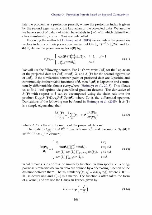
Chapter 3. Projection Pursuit Based on Spectral Connectivity
late the problem as a projection pursuit, where the projection index is givenby the second eigenvalue of the Laplacian of the projected data. We assumewe have a set of N data, l of which have labels in −1,+1 which define theirclass membership, and u=N− l are unlabelled.
Following the method of Hofmeyr et al. (2015) we formulate the projectionvectors in terms of their polar coordinates. Let Θ=[0,π)d−2× [0,2π) and forθθθ∈Θ, define the projection vector v(θθθ) by,
v(θθθ)i=
cos(θθθi)∏i−1j=1 sin(θθθ j), i=1, . . . ,d−1
∏d−1j=1 sin(θθθ j), i=d.
(3.41)
We will use the following notation. For θθθ∈Θ, we write L(θθθ) for the Laplacianof the projected data set P(θθθ) :=v(θθθ) ·X, and λ2(θθθ) for the second eigenvalueof L(θθθ). If the similarities between pairs of projected data are Lipschitz andcontinuously differentiable functions of θθθ, then λ2(θθθ) is Lipschitz and contin-uously differentiable almost everywhere (Hofmeyr et al., 2015). This allowsus to find local optima via generalised gradient descent. The derivative ofλ2(θθθ) with respect to θθθ can be decomposed using the chain rule into theproduct DP(θθθ)λ2(θθθ)Dv(θθθ)P(θθθ)Dθθθv(θθθ), where D·· is the differential operator.Derivations of the following can be found in Hofmeyr et al. (2015). If λ2(θθθ)is a simple eigenvalue, then
∂λ2(θθθ)
∂P(θθθ)k=
12 ∑
ij(ui−uj)
2 ∂A(θθθ)ij
∂P(θθθ)k, (3.42)
where A(θθθ) is the affinity matrix of the projected data set.The matrix Dv(θθθ)P(θθθ)∈RN×d has i-th row x>i , and the matrix Dθθθv(θθθ)∈
Rd×(d−1) has i, j-th element,
∂v(θθθ)i∂θθθ j
=
0, i< j−sin(θθθ j)∏
j−1k=1 sin(θθθk), i= j<d
cos(θθθ j)cos(θθθi)∏k<i,k 6=j sin(θθθk), j< i<d
cos(θθθ j)∏k 6=j sin(θθθk), i=d.
(3.43)
What remains is to address the similarity function. Within spectral clustering,pairwise similarities between data are defined by a decreasing function of thedistance between them. That is, similarity(xi,xj)=k(d(xi,xj)), where k :R+→R+ is decreasing and d(·, ·) is a metric. The function k often takes the formof a kernel, and we use the Gaussian kernel, given by
k(x)=exp(− x2
2
). (3.44)
106
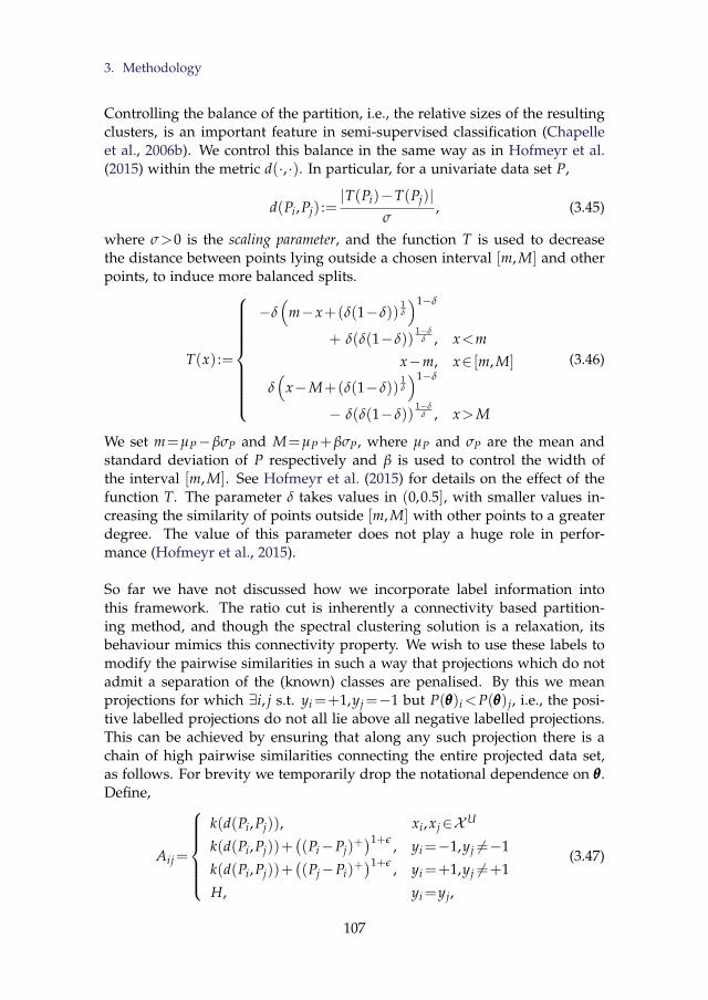
3. Methodology
Controlling the balance of the partition, i.e., the relative sizes of the resultingclusters, is an important feature in semi-supervised classification (Chapelleet al., 2006b). We control this balance in the same way as in Hofmeyr et al.(2015) within the metric d(·, ·). In particular, for a univariate data set P,
d(Pi,Pj) :=|T(Pi)−T(Pj)|
σ, (3.45)
where σ>0 is the scaling parameter, and the function T is used to decreasethe distance between points lying outside a chosen interval [m, M] and otherpoints, to induce more balanced splits.
T(x) :=
−δ(
m−x+(δ(1−δ))1δ
)1−δ
+ δ(δ(1−δ))1−δ
δ , x<mx−m, x∈ [m, M]
δ(
x−M+(δ(1−δ))1δ
)1−δ
− δ(δ(1−δ))1−δ
δ , x>M
(3.46)
We set m=µP−βσP and M=µP+βσP, where µP and σP are the mean andstandard deviation of P respectively and β is used to control the width ofthe interval [m, M]. See Hofmeyr et al. (2015) for details on the effect of thefunction T. The parameter δ takes values in (0,0.5], with smaller values in-creasing the similarity of points outside [m, M] with other points to a greaterdegree. The value of this parameter does not play a huge role in perfor-mance (Hofmeyr et al., 2015).
So far we have not discussed how we incorporate label information intothis framework. The ratio cut is inherently a connectivity based partition-ing method, and though the spectral clustering solution is a relaxation, itsbehaviour mimics this connectivity property. We wish to use these labels tomodify the pairwise similarities in such a way that projections which do notadmit a separation of the (known) classes are penalised. By this we meanprojections for which ∃i, j s.t. yi=+1,yj=−1 but P(θθθ)i<P(θθθ)j, i.e., the posi-tive labelled projections do not all lie above all negative labelled projections.This can be achieved by ensuring that along any such projection there is achain of high pairwise similarities connecting the entire projected data set,as follows. For brevity we temporarily drop the notational dependence on θθθ.Define,
Aij=
k(d(Pi,Pj)), xi,xj∈XU
k(d(Pi,Pj))+((Pi−Pj)
+)1+ε , yi=−1,yj 6=−1
k(d(Pi,Pj))+((Pj−Pi)
+)1+ε , yi=+1,yj 6=+1
H, yi=yj,
(3.47)
107
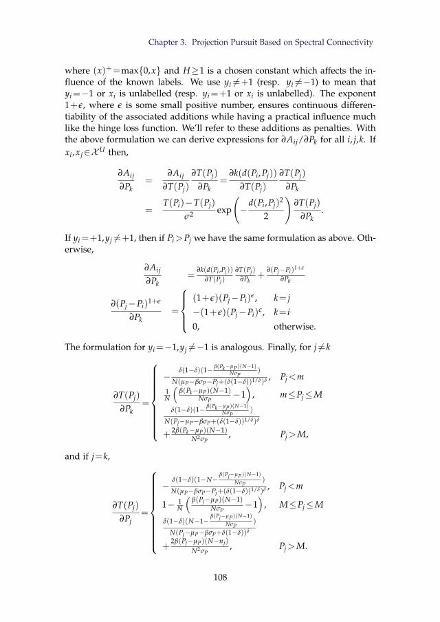
Chapter 3. Projection Pursuit Based on Spectral Connectivity
where (x)+=max0,x and H≥1 is a chosen constant which affects the in-fluence of the known labels. We use yi 6=+1 (resp. yi 6=−1) to mean thatyi=−1 or xi is unlabelled (resp. yi=+1 or xi is unlabelled). The exponent1+ε, where ε is some small positive number, ensures continuous differen-tiability of the associated additions while having a practical influence muchlike the hinge loss function. We’ll refer to these additions as penalties. Withthe above formulation we can derive expressions for ∂Aij/∂Pk for all i, j,k. Ifxi,xj∈XU then,
∂Aij
∂Pk=
∂Aij
∂T(Pj)
∂T(Pj)
∂Pk=
∂k(d(Pi,Pj))
∂T(Pj)
∂T(Pj)
∂Pk
=T(Pi)−T(Pj)
σ2 exp
(−
d(Pi,Pj)2
2
)∂T(Pj)
∂Pk.
If yi=+1,yj 6=+1, then if Pi>Pj we have the same formulation as above. Oth-erwise,
∂Aij
∂Pk=
∂k(d(Pi ,Pj))
∂T(Pj)
∂T(Pj)
∂Pk+
∂(Pj−Pi)1+ε
∂Pk
∂(Pj−Pi)1+ε
∂Pk=
(1+ε)(Pj−Pi)
ε, k= j
−(1+ε)(Pj−Pi)ε, k= i
0, otherwise.
The formulation for yi=−1,yj 6=−1 is analogous. Finally, for j 6=k
∂T(Pj)
∂Pk=
−δ(1−δ)(1− β(Pk−µP)(N−1)
NσP)
N(µP−βσP−Pj+(δ(1−δ))1/δ)δ , Pj<m
1N
(β(Pk−µP)(N−1)
NσP−1)
, m≤Pj≤M
δ(1−δ)(1− β(Pk−µP)(N−1)NσP
)
N(Pj−µP−βσP+(δ(1−δ))1/δ)δ
+ 2β(Pk−µP)(N−1)N2σP
, Pj>M,
and if j=k,
∂T(Pj)
∂Pj=
−δ(1−δ)(1−N−
β(Pj−µP)(N−1)NσP
)
N(µP−βσP−Pj+(δ(1−δ))1/δ)δ , Pj<m
1− 1N
(β(Pj−µP)(N−1)
NσP−1)
, M≤Pj≤M
δ(1−δ)(N−1−β(Pj−µP)(N−1)
NσP)
N(Pj−µP−βσP+δ(1−δ))δ
+2β(Pj−µP)(N−nj)
N2σP, Pj>M.
108
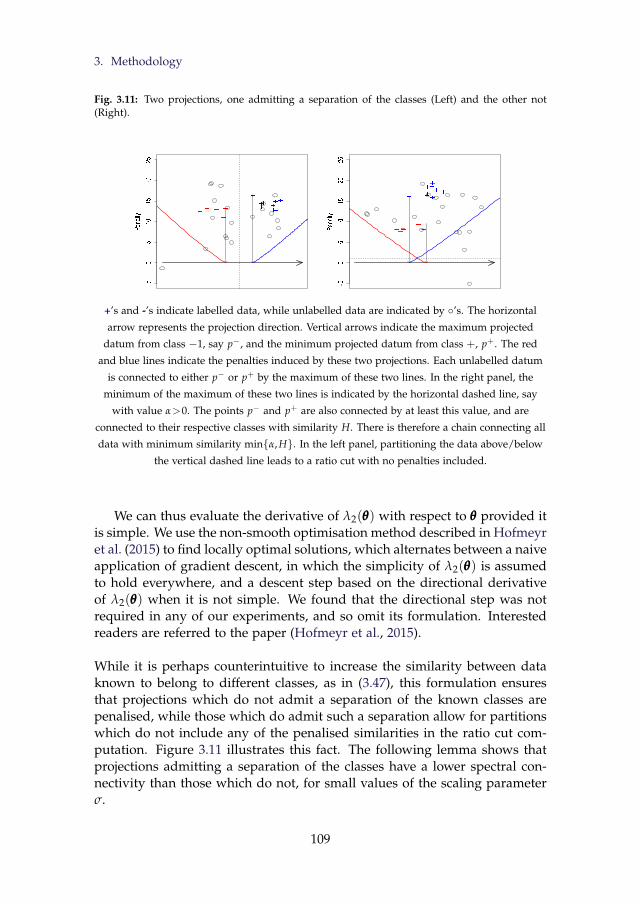
3. Methodology
Fig. 3.11: Two projections, one admitting a separation of the classes (Left) and the other not(Right).
+’s and -’s indicate labelled data, while unlabelled data are indicated by ’s. The horizontal
arrow represents the projection direction. Vertical arrows indicate the maximum projected
datum from class −1, say p−, and the minimum projected datum from class +, p+. The red
and blue lines indicate the penalties induced by these two projections. Each unlabelled datum
is connected to either p− or p+ by the maximum of these two lines. In the right panel, the
minimum of the maximum of these two lines is indicated by the horizontal dashed line, say
with value α>0. The points p− and p+ are also connected by at least this value, and are
connected to their respective classes with similarity H. There is therefore a chain connecting all
data with minimum similarity minα, H. In the left panel, partitioning the data above/below
the vertical dashed line leads to a ratio cut with no penalties included.
We can thus evaluate the derivative of λ2(θθθ) with respect to θθθ provided itis simple. We use the non-smooth optimisation method described in Hofmeyret al. (2015) to find locally optimal solutions, which alternates between a naiveapplication of gradient descent, in which the simplicity of λ2(θθθ) is assumedto hold everywhere, and a descent step based on the directional derivativeof λ2(θθθ) when it is not simple. We found that the directional step was notrequired in any of our experiments, and so omit its formulation. Interestedreaders are referred to the paper (Hofmeyr et al., 2015).
While it is perhaps counterintuitive to increase the similarity between dataknown to belong to different classes, as in (3.47), this formulation ensuresthat projections which do not admit a separation of the known classes arepenalised, while those which do admit such a separation allow for partitionswhich do not include any of the penalised similarities in the ratio cut com-putation. Figure 3.11 illustrates this fact. The following lemma shows thatprojections admitting a separation of the classes have a lower spectral con-nectivity than those which do not, for small values of the scaling parameterσ.
109
Chapter 3. Projection Pursuit Based on Spectral Connectivity
Lemma 17 Let k be non-increasing, Lipschitz and satisfy k(x)∈o(x−(1+ε)) as x→∞. Let θθθ1 be such that minP(θθθ1)i|yi=+1>maxP(θθθ1)j|yj=−1. Then ∃σ′>0s.t. for any 0<σ<σ′ and θθθ2 s.t. minP(θθθ2)i|yi=+1≤maxP(θθθ2)j|yj=−1 wehave λ2(θθθ1)<λ2(θθθ2).
We see then that the formulation given in (3.47) does indeed induce apenalty, and the penalty forces the optimal solution to admit a separation ofthe classes if σ is small enough, assuming that the classes can be separated.We can extend the above result to show that the optimal projection convergesto the vector normal to the TSVM solution, as σ→0+. We discuss the resultin the context of a constrained solution, i.e., one which induces a balancedpartition by intersecting a scaled covariance ellipsoid. The result holds for allvalues of β, and so setting β arbitrarily large proves the result relative to theoriginal TSVM problem.
Lemma 18 Suppose ∃v∈Rd,b∈R s.t. yi(v ·xi−b)>0 for all i∈1, . . . , l. Letk :R+→R+ satisfy the following:
1. k is non-increasing
2. k is Lipschitz
3. limx→∞ k(x+ε)/k(x)=0 for all ε>0
4. k(x)∈o(x−(1+ε)) as x→∞.
For σ,δ>0 define θθθσ,δ=argminθθθ∈Θλ2(θθθ,σ,δ), where λ2(θθθ,σ,δ) is the same as λ2(θθθ)from before but with an explicit dependence on σ and δ. Let (v?,b?) define thelargest margin hyperplane which correctly classifies all labelled data and satisfiesm<b?< M, where m lies halfway between µv? ·X−βσv? ·X and the smallest elementof P(θθθ?) above µv? ·X−βσv? ·X and similarly M lies halfway between µv? ·X+βσv? ·Xand the largest element of P(θθθ?) below µv? ·X+βσv? ·X . Then,
limσ,δ→0+
v(θθθσ,δ)=v?
The distinction between m and µv? ·X−βσv? ·X , and analogously for M, is notof much practical concern, but is important for proving the associated theory.The reader may refer to Hofmeyr et al. (2015) for additional discussion.
3.1 Computational Complexity
It is clear to see that the proposed method has the same computational com-plexity as the corresponding unsupervised projection pursuit given by Hofmeyret al. (2015), since the difference between the semi-supervised approach de-scribed herein and the unsupervised problem lies only in the modification
110
4. Experiments
of pairwise similarities, which does not affect the computational complexity.Hofmeyr et al. (2015) have shown the the computational cost for each evalu-ation of the projection index is O(N(N+d)), and each gradient computationhas complexity O(N(N+d(d−1))). The total complexity of the method istherefore O(N(N+d(d−1))t), where t is the number of steps in the gradientdescent.
4 Experiments
In this section we evaluate the performance of the proposed method, whichwe will refer to as Semi-Supvervised Spectral Connectivity Projection Pur-suit (S3CP2), on classification data sets taken from the UCI Machine LearningRepository (UCIMLR).6 and benchmark data sets for semi-supervised classi-fication.7 For each UCIMLR data set we generated 30 sets of labels, 10 foreach of the sizes 2%, 10% and 25% the total number of data. The label setswere generated uniformly at random, however sets which did not containat least one label from each class were rejected and replaced with another.For the data sets taken from Chapelle et al. (2006b) we used the same 24 labelsets, 12 for each of 10 and 100 labels. The UCIMLR data sets considered were:Mammographic Mass (Mam.): Distinguish benign from malignant massesfound during mammography screening. Voters (Vote.): Determine politicalparty affiliation from votes made by US congress members. Breast Cancer(Canc.): Distinguish benign from malignant tumour masses, given physicalcharacteristics. Ionosphere (Iono.): Distinguish radio signals which show ev-idence of structure in the ionosphere from those which don’t. Parkinsons(Park.): A range of biomedical voice measurements used to determine thepresence of Parkinson’s disease. The data sets taken from Chapelle et al.(2006b) were: g241c: A mixture of 2 Gaussian distributions for which thecluster assumption holds. g241d: A 4 component Gaussian mixture in whichcluster structure is misleading for class membership. Digit1: Artificially gen-erated images of the digit “1" varied by translation, ratation, line thicknessand length, obscured to increase difficulty. Class boundary at the 0 rotationangle. The cluster assumption holds. USPS: U.S. Postal Service handwrittendigits. Digits “2" and “5" form class +1 with the remaining digits form-ing class −1. The images are obscured using the same transformation asfor Digit1. BCI: A brain-computer interface experiment in which a subjectimagined movements with their right, class +1, and left hand, class −1. Thefeatures are EEG readings taken during the experiment.
6M. Lichman. UCI Machine Learning Respository http://archive.ics.uci.edu/ml. Irvine,CA. University of California, School of Information and Computer Science. 2013
7A selection of data sets used in Chapelle et al. (2006b)http://olivier.chapelle.cc/ssl-book/benchmarks.html.
111
Chapter 3. Projection Pursuit Based on Spectral Connectivity
We compare performance with a standard SVM8 trained only on the la-belled data, and Semi-Supervised SVM (S3VM)9. We use the linear kernel forSVM and S3VM since this provides the most meaningful comparison withour proposed method. Non-linear separators are possible for our methodby an explicit embedding of the data within the kernel space, as in Chapelleet al. (2006a). For SVM we use the default parameters given in the package.For S3VM we initialised using SVM and built classifiers for each of 5 values ofC?, which determines the penalty for the unlabelled data violating the largemargin, in each experiment using the UCIMLR data sets. We then report thehighest average performance of those 5 for each case. For the data sets aris-ing from Chapelle et al. (2006b) we use the results presented there. For S3CP2
we initialise the projection pursuit using the SVM solution. For the UCIMLRdata sets we set β=1.5, σ=0.3nn0.99/
√d where nn0.99 is the 99th centile of the
nearest neighbour distances in the data and d is the dimension, and H=u/l,the ratio of the number of unlabelled and labelled data. The data sets takenfrom Chapelle et al. (2006b) are more challenging, and we selected σ and βfrom the sets 0.1nn0.99/
√d,0.5nn0.99/
√d and 0.5,1.5 respectively using
cross validation.Tables 3.7 and 3.8 report the average classification accuracy over the dif-
ferent label sets. The highest average performance is highlighted in bold.The proposed method achieves the highest average performance in roughlyhalf of the cases considered, and is competitive with the highest performingmethod in almost all. Importantly the method achieved higher performancethan linear S3VM in the majority of applications.
Parameter tuning is a very difficult task in semi-supervised classifica-tion (Chapelle et al., 2006b), and though our method contains numerousparameters, the majority do not play a significant role in its performance.The parameter σ, and to a lesser extent β, plays the most crucial role in theperformance of the method, and determining an appropriate value is neces-sary for the successful application of the method. We used a simple referencerule which has worked well on many of the examples considered, but believeconsiderable improvements can be made if a more principled tuning methodis employed.
5 Conclusions
We propose a new method for semi-supervised classification, which is basedon learning the optimal univariate subspace to perform a binary partition ofthe projected data set using semi-supervised spectral clustering. The labels
8We use the R package e1071, which implements the libSVM library9We use the SVM-light implementation of T. Joachims available at
http://svmlight.joachims.org/
112
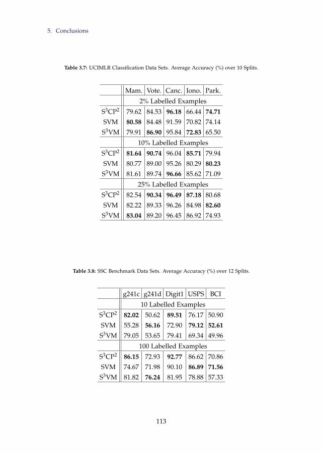
5. Conclusions
Table 3.7: UCIMLR Classification Data Sets. Average Accuracy (%) over 10 Splits.
Mam. Vote. Canc. Iono. Park.
2% Labelled Examples
S3CP2 79.62 84.53 96.18 66.44 74.71SVM 80.58 84.48 91.59 70.82 74.14
S3VM 79.91 86.90 95.84 72.83 65.50
10% Labelled Examples
S3CP2 81.64 90.74 96.04 85.71 79.94
SVM 80.77 89.00 95.26 80.29 80.23S3VM 81.61 89.74 96.66 85.62 71.09
25% Labelled Examples
S3CP2 82.54 90.34 96.49 87.18 80.68
SVM 82.22 89.33 96.26 84.98 82.60S3VM 83.04 89.20 96.45 86.92 74.93
Table 3.8: SSC Benchmark Data Sets. Average Accuracy (%) over 12 Splits.
g241c g241d Digit1 USPS BCI
10 Labelled Examples
S3CP2 82.02 50.62 89.51 76.17 50.90
SVM 55.28 56.16 72.90 79.12 52.61S3VM 79.05 53.65 79.41 69.34 49.96
100 Labelled Examples
S3CP2 86.15 72.93 92.77 86.62 70.86
SVM 74.67 71.98 90.10 86.89 71.56S3VM 81.82 76.24 81.95 78.88 57.33
113
Chapter 3. Projection Pursuit Based on Spectral Connectivity
of the training data are incorporated into the model in such a way that theglobally optimal solution must admit a separation of the classes within thetraining data, if such a solution exists, and for all scaling parameters close tozero. We also show that asymptotically this optimal solution converges to thesubspace normal to the optimal TSVM hyperplane, as the scaling parameteris reduced to zero, thereby providing a theoretical connection between ourproposed method and popular semi-supervised classification methodology.Experimental results indicate the proposed method is competitive with state-of-the-art TSVM implementation in terms of classification accuracy.
Appendix. Proofs
The following lemma is useful for proving Lemmas 17 and 18.
Lemma 19 Let k be non-increasing and Lipschitz with constant K, and let k(0)=1.For θθθ∈Θ let
∆θθθ =[mθθθ , Mθθθ ]∩ [maxP(θθθ)i|yi=−1,minP(θθθ)j|yj=+1],
where
mθθθ =µP(θθθ)−βσP(θθθ)+minP(θθθ)∩ [µP(θθθ)−βσP(θθθ),∞)
2
Mθθθ =µP(θθθ)+βσP(θθθ)+maxP(θθθ)∩(−∞,µP(θθθ)+βσP(θθθ)]
2.
Let σ′= K(1+ε)1/1+ε . If ∆θθθ 6=∅ then set Gθθθ =maxb∈∆θθθ
mini∈1,...N |P(θθθ)i−b|. Then
for σ≤σ′ we have,
λ2(θθθ)≥min
19|X|3 k
(2Gθθθ +δD
σ
),
19|X|
( σ
K
)1+ε
,
where D=maxDiam(X),Diam(X)1−δ. If ∆θθθ =∅ then we simply have
λ2(θθθ)≥1
9|X|
( σ
K
)1+ε,
for all σ≤σ′.
Proof Since k has Lipschitz constant K we have
k(x/σ)+x1+ε≥(k(0)− Kσ
x)++x1+ε=(1− Kσ
x)++x1+ε.
Since σ≤σ′= K(1+ε)1/1+ε we can show that (1− K
σ x)++x1+ε≥(
σK)1+ε for all
x≥0.
114

5. Conclusions
First consider the case ∆θθθ =∅. For each j, we must have either P(θθθ)j≤maxP(θθθ)i|yi=−1 or P(θθθ)j≥minP(θθθ)i|yi=+1. Let I and J be the in-dices corresponding to maxP(θθθ)i|yi=−1 and minP(θθθ)i|yi=+1 respec-tively. Therefore, for each j s.t. xj∈XU either
AjI≥k(|P(θθθ)j−P(θθθ)I)|/σ)+ |P(θθθ)j−P(θθθ)I |1+ε≥( σ
K
)1+ε
orAjJ≥k(|P(θθθ)j−P(θθθ)J |/σ)+ |P(θθθ)j−P(θθθ)J |1+ε≥
( σ
K
)1+ε.
In addition we have
AI J≥k(|P(θθθ)I−P(θθθ)J |/σ)+ |P(θθθ)I−P(θθθ)J |1+ε≥( σ
K
)1+ε,
and for each j s.t. yj=+1 and i s.t. yi=−1 we similarly have AjI , Ai J≥(σK)1+ε. Now, let u be the second eigenvector of L(θθθ), then ‖u‖=1,u⊥1 and
so ∃i, j s.t. ui−uj≥ 1√|X|
. If |uI−uJ |≤ 13√|X|
then either |ui−uI |≥ 13√|X|
and
|ui−uJ |≥ 13√|X|
or |uj−uI |≥ 13√|X|
and |uj−uJ |≥ 13√|X|
. Then,
λ2(L(θθθ))=u ·L(θθθ)u= 12 ∑
k,lAkl(uk−ul)
2
≥AiI(ui−uI)2+Ai J(ui−uJ)
2+AjI(uj−uI)2+AjJ(uj−uJ)
2
≥ 19|X|
( σ
K
)1+ε
in all possible cases, since(
σK)1+ε≤1≤H. On the other hand we have |uI−
uJ |≥ 13√|X|
and so λ2(L(θθθ))≥AI J(uI−uJ)2≥(
σK)1+ε /9|X| as required.
Now consider the case ∆θθθ 6=∅. Define u, I, J as above. If
maxi,j:P(θθθ)i ,P(θθθ)j∈[P(θθθ)I ,P(θθθ)J ]
(ui−uj)≤1
3√|X|
,
then since ∃i, j with ui−uj≥ 1√|X|
we must have either P(θθθ)i 6∈ [P(θθθ)I ,P(θθθ)J ]
and |ui−uI |≥ 13√|X|
and |ui−uJ |≥ 13√|X|
or P(θθθ)j 6∈ [P(θθθ)I ,P(θθθ)J ] and |uj−
uI |≥ 13√|X|
and |uj−uJ |≥ 13√|X|
. Suppose w/o loss of generality that P(θθθ)i
satisfies these three conditions. If xi∈XU then since P(θθθ)i 6∈ [P(θθθ)I ,P(θθθ)J ] wehave either AiI≥
(σK)1+ε or Ai J≥
(σK)1+ε and the result follows similarly to
above. If xi∈X L then either AiI =1 or Ai J =1≥(
σK)1+ε, and again the result
follows as above. If instead we have
maxi,j:P(θθθ)i ,P(θθθ)j∈[P(θθθ)I ,P(θθθ)J ]
(ui−uj)>1
3√|X|
,
115
Chapter 3. Projection Pursuit Based on Spectral Connectivity
then the result follows analogously to (Hofmeyr et al., 2015, Lemma 2), withthe addition of the factor 1
3 on the distance between elements of u in consid-eration.
Proof of Lemma 17 Let Gθθθ1>0 be defined as in Lemma 19, and let b be the
corresponding point at which the distance is maximised. Let L and R be thenumber of projected data lying to the left and right of b respectively. Then,since spectral clustering solves the relaxation of the ratio cut, we have
λ2(θθθ1)≤1|X|min
C⊂X∑
i,j:xi∈Cxj 6∈C
A(θθθ1)ij
(1|C|+
1|X\C|
)
≤ 1|X| ∑
i,j:P(θθθ1)i<bP(θθθ1)j>b
k(d(P(θθθ1)i,P(θθθ1)j))
(1L+
1R
)
≤k(2Gθθθ1/σ).
For any θθθ2 s.t. ∆θθθ2 defined as in Lemma 19 is empty, we have
λ2(θθθ1)
λ2(θθθ2)≤9|X|K1+εk(2Gθθθ1
/σ)σ−(1+ε)
This right hand side is independent of θθθ2, and converges to 0 as σ→0+ sincek(x)∈o(x−(1+ε)) as x→∞. Therefore the result holds.
Proof of Lemma 18 By Lemma 17 we know that ∃σ′>0 s.t. 0<σ<σ′⇒∆θθθσ,δ6=∅, where ∆θθθ is as in Lemma 19. Take γ>0. It has been shown Pavlidis
et al. (2015) that ∃mγ>0 s.t. for w∈Rd and c∈R one has ‖(w,c)/‖w‖−(v?,b?)‖>γ⇒margin(w/‖w‖,c/‖w‖)<margin(v?,b?)−mγ. Let θθθ? be suchthat v(θθθ?)=v? so that margin(v?,b?)=Gθθθ? , where Gθθθ is as in Lemma 19. Asin the proof of Lemma 17 we have
λ2(θθθ?)≤k(2Gθθθ?/σ).
In addition, for small enough σ>0 we have
19|X|3 k
(2G+δD
σ
)<
19|X|
( σ
K
)1+ε
holding uniformly in δ>0 for any G>0, where K,D are as in Lemma 19.Therefore, for small σ,δ we have
λ2(θθθσ,δ)≥1
9|X|3 k(2Gθθθσ,δ
+δDσ
),
116

5. Conclusions
and hence1
9|X|3 k(2Gθθθσ,δ
+δDσ
)≤k(
2Gθθθ?
σ
)since λ2(θθθσ,δ)≤λ2(θθθ
?). Now, take δ′ s.t. δ′D<mγ
2 . Since limx→∞ k(x+ε)/k(x)=0 for all ε>0, ∃σ′>0 s.t. 9|X|3K(2Gθθθ?/σ)<k((2Gθθθ?−
mγ
2 )/σ) for all σ<σ′.For σ<σ′,δ<δ′ we have,
k
(2Gθθθσ,δ
+mγ
2
σ
)≤k(2Gθθθσ,δ
+δDσ
)≤9|X|3k
(2Gθθθ?
σ
)≤k
(2Gθθθ?−
mγ
2σ
)⇒2Gθθθσ,δ
+mγ
2≥2Gθθθ?−
mγ
2
⇒ maxb∈∆θθθσ,δ
margin(v(θθθσ,δ),b)≥margin(v?,b?)−mγ
2
⇒‖(v(θθθσ,δ),b)−(v?,b?)‖≤γ
⇒‖v(θθθσ,δ)−v?‖≤γ
Since γ>0 was arbitrary and the above holds for all σ<σ′,δ<δ′ we musthave limσ,δ→0+ v(θθθσ,δ)=v? as required.
117
Chapter 4
Clustering by Minimum CutHyperplanes
Abstract
Minimum normalised graph cuts are highly effective ways of partitioning unlabeleddata, having been made popular by the success of spectral clustering. This workpresents a novel method for learning hyperplane separators which minimise thisgraph cut objective. The optimisation problem associated with the proposed methodcan be formulated as a sequence of univariate subproblems, in which the optimal hy-perplane orthogonal to a given vector is determined. These subproblems can be solvedin log-linear time, by exploiting the trivial factorisation of the exponential function.Experimentation suggests that the empirical runtime of the overall algorithm is alsolog-linear in the number of data. This compares favourably with existing methodsbased on normalised graph cuts.
Asymptotic properties of the minimum cut hyperplane, both for a finite sample,and for an increasing sample assumed to arise from an underlying probability distri-bution are discussed. In the finite sample case the minimum cut hyperplane convergesto the maximum margin hyperplane as the scaling parameter is reduced to zero.
Applying the proposed methodology, both for fixed scaling, and the large mar-gin asymptotes, is shown to produce high quality clustering models in comparisonwith state-of-the-art clustering algorithms in experiments using a large collection ofbenchmark datasets.
1 Introduction
Clustering is fundamental to many statistical and machine learning applica-tions, and deals with partitioning sets of data into groups which are believed
118
1. Introduction
to be related, without any explicit prior information regarding the group as-sociations of any of the data. Such applications arise in diverse fields fromcomputer vision (Tatiraju and Mehta, 2008), to bio-informatics (Sturn et al.,2002) to marketing (Punj and Stewart, 1983).
Common to many clustering methods is the notion of similarity, and theclustering problem can be abstractly stated as follows: determine a parti-tion of a data set such that data within groups are more similar than databetween groups. The popular K-means algorithm, as well as other centroidbased methods, define groups of similar data by how they cluster around asmall number of cluster centroids (Leisch, 2006). Density based clusteringmethods form groups of data which fall in connected regions of high datadensity. In the statistics literature these high density clusters are interpreted viathe level sets of an assumed underlying probability density (Hartigan, 1975).A third approach, and that which forms the motivation for this work, is clus-tering by graph cuts. This approach provides a highly principled frameworkwithin which to address the notion of similarity, as the objective which drivesthe partitioning deals explicitly with the pairwise similarities between data.The minimum graph cut problem directly minimises the sum of the similar-ities between data belonging to different groups in a partition. Normalisa-tions of the graph cut objective are used to emphasise partitions which havehigh within cluster similarity, and to induce more balanced partitions. Thenormalised graph cut problem, however, is NP-hard (Wagner and Wagner,1993). The relaxations given by spectral clustering (Hagen and Kahng, 1992;Shi and Malik, 2000) mitigate this problem, however the resulting complexityremains O(n2), where n is the number of data. Further approximations havebeen developed to allow these methods to be applied to larger problems.The Nyström method generates a low rank approximation of the matrix ofpairwise similarities before applying spectral clustering to this approximateaffinity matrix (Fowlkes et al., 2004). An alternative approach reduces the sizeof the affinity matrix by first performing a coarse clustering of the data us-ing a comparatively simple method (e.g. K-means), and then computing thepairwise similarities between the resulting clusters (Yan et al., 2009).
This paper introduces a new divisive hierarchical clustering method, inwhich each partition in the hierarchy is induced by a hyperplane separa-tor. Each separating hyperplane is the solution to an optimisation problemwhich is motivated by the graph partitioning objective, and minimises thenormalised graph cut measured across the hyperplane. Restricting attentionto hyperplane based partitions, while slightly limiting in the fact that theresulting clusters must be linearly separated, offers considerable computa-tional benefits. Moreover, the empirical performance of the method is highlycompetitive with state-of-the-art clustering algorithms in terms of clusteringaccuracy. The formulation presented can be viewed as a sequence of univari-ate subproblems, each of which can be solved in O(n logn) time, where n is
119
Chapter 4. Clustering by Minimum Cut Hyperplanes
the number of data. An empirical study indicates that the overall algorithmalso runs in O(n logn) time, allowing for the application of the proposed ap-proach to large problems without the need for approximations. Moreover,the empirical runtime of the proposed method compares favourably with theapproximate spectral clustering methods.
Asymptotic properties of the normalised cut across a hyperplane are ex-plored, showing desirable qualities in the context of the non-parametric sta-tistical formulation of the clustering problem (Hartigan, 1975). In particularthe optimal hyperplane will both have low density integral, therefore passingthrough regions of low density, and also will tend to separate the modes ofthe underlying probability density, which correspond to high density clus-ters. Additionally the optimal hyperplane for the proposed objective, eval-uated on a fixed data set, is shown to be connected with maximum marginhyperplane separators, and the proposed methodology can be modified tofind large margin hyperplanes practically. This is an important result as max-imum margin clustering has gained considerable attention in recent years forits good performance in many application areas including image analysis,and text mining (Xu et al., 2004; Zhang et al., 2009). Experiments with theproposed approach for finding large margin hyperplanes indicates that it ishighly competitive with existing methods for the problem. In addition, theapproach significantly reduces the computation time required to find largemargin hyperplanes.
The remainder of this paper is organised as follows. Section 2 intro-duces graph partitioning and presents the proposed problem formulation.The asymptotic properties of the proposed method are investigated and dis-cussed. In Section 3 the methodology for solving the proposed problem ispresented in detail. Section 4 presents the results from extensive experimentson benchmark data sets for clustering. Finally, concluding remarks are givenin Section 5.
2 Problem Formulation
This section presents an introduction to graph partitioning by (normalised)graph cuts, and provides the hyperplane based formulation which formsthe focus of this paper. A theoretical discussion of two popular normalisa-tion techniques, RatioCut (Hagen and Kahng, 1992) and normalised cut, orNCut (Shi and Malik, 2000), is presented. The conclusion is, at least in rela-tion to the proposed hyperplane formulation, that NCut has preferable char-acteristics in the context of data clustering. Following this analysis, the NCutapproach is adopted as the focus of the subsequent methodology presentedin the next section. In addition, a connection between the optimal hyper-plane based on the NCut objective and the maximum margin hyperplane is
120

2. Problem Formulation
established, showing that as the scaling parameter in the Ncut formulationis reduced to zero, the optimal NCut hyperplane converges to the maximummargin hyperplane through the data.
2.1 Background on Normalised Graph Cuts
The graph cut problem for data partitioning is given as follows. For a setof data X =x1, ...,xn in Rd, define the graph G(X )=(X ,E) with verticesequal to the elements of X and undirected edges assuming weights equal tothe similarity between pairs of data in X . In practice the similarity betweenpoints relates to their relative spatial relationship, in that pairs of data whichare further apart tend to be given lower similarity value than those which arecloser. The information in G(X ) can be represented by the affinity matrixA(X )∈Rn×n which has i, j-th element equal to the similarity between dataxi and xj. From the affinity matrix one can define the diagonal degree matrixD(X )∈Rn×n with i-th diagonal element equal to ∑n
j=1 A(X )i,j.Now, for a subset C⊂X the graph cut between C and X \C is given by
the sum of the similarities between data in C and those in X \C. Formally,
Cut(C,X \C) := ∑i,j:xi∈C
xj 6∈C
A(X )i,j. (4.1)
Minimising (4.1) over all subsets C⊂X can be performed in polynomialtime (Stoer and Wagner, 1997), however this approach tends to result in eitherC or X \C containing very few points (von Luxburg, 2007). Normalisationsare used to induce more balanced partitions. Two such normalisations arecommon, known as RatioCut and NCut, defined as follows,
RatioCut(C,X \C) :=Cut(C,X \C)(
1|C|+
1|X \C|
)(4.2)
NCut(C,X \C) :=Cut(C,X \C)
1∑
i:xi∈CD(X )i
+1
∑i:xi 6∈C
D(X )i
. (4.3)
The minimisation of both RatioCut and NCut over all subsets C⊂X is NP-hard (Wagner and Wagner, 1993). Considering only hyperplane based parti-tions, however, results in a far simpler problem, as will be discussed in theremainder.
2.2 Normalised Cuts Across Hyperplanes
A hyperplane in Rd is a translated subspace of co-dimension 1, and can beparameterised by a unit vector v∈Rd,‖v‖=1, and scalar b∈R as the set,
H(v,b) :=x∈Rd|v ·x=b. (4.4)
121
Chapter 4. Clustering by Minimum Cut Hyperplanes
Notice that the unit-vector v defines the subspace normal to the hyperplane.Henceforth denote the set of unit norm vectors in Rd by Bd.
Hyperplanes induce a binary partition of Rd, and therefore of any data setresiding in Rd, based on the negative/non-negative elements of the subspace,i.e., separating those x∈Rd s.t. v ·x<b from those satisfying v ·x≥b. Thefollowing notation will be used to define these half spaces,
H(v,b)− :=x∈Rd|v ·x<b (4.5)
H(v,b)+ :=x∈Rd|v ·x≥b. (4.6)
Hyperplane based clustering algorithms have been successfully applied in anumber of application areas, including text mining, microarray analysis, andimage segmentation (Boley, 1998; Tasoulis et al., 2010; Zhang et al., 2009).
Connections between clustering by normalised graph cuts and the so-calledlow density separation assumption have been established (Narayanan et al.,2006), in that the value of the normalised cut is asymptotically related tothe integrated density along the surface inducing the cut. The low densityseparation assumption states that clusters are separated by contiguous re-gions of relatively low density, and is equivalent to the definition of clustersas high density regions which underlies density clustering. Within the non-parametric statistical approach to clustering, high density clusters may beassociated with the level sets of an (assumed) underlying probability den-sity (Hartigan, 1975). A separating hyperplane for clustering should there-fore, as well as possible, separate regions of high density (it should separateclusters) while avoiding intersection with any such high density regions (in-dividual clusters should remain intact after the partition). In particular, thesurface integral of the underlying probability density along the hyperplaneshould be low, while there should exist regions of high density lying bothsides of the hyperplane. A further theoretical investigation into the asymp-totic properties of normalised cuts, and their relationship to high densityclustering, is presented below. Particular attention is paid to hyperplane sep-arators, and in relation to the criteria set out above.
For a random variable X in Rd with probability density p :Rd→R+, the sur-face integral of the density along a hyperplane, H(v,b), is simply the valueof the marginal density of the univariate random variable v ·X evaluated atb. Henceforth, for v∈Bd, the marginal density of v ·X will be written as pv,i.e.,
pv(b)=∫
x∈H(v,b)p(x)dx. (4.7)
While exceptions exist, in general we find that if a hyperplane H(v,b) sep-arates modes in the marginal density pv then there tend to exist modes in the
122
2. Problem Formulation
full dimensional joint density, p, on both sides of H(v,b). A natural assump-tion when clustering data assumed to arise from an underlying probabilitydistribution is that the distribution represents a mixture of comparativelysimple components. If these components are, for example, elliptical, then ahyperplane separating modes in the marginal density will always intersectthe convex hull of the modes of the individual components, as shown in thefollowing simple proposition.
Proposition 20 Let p(x)=∑ki=1 πi pi(x), where ∑k
i=1 πi=1,πi>0, i=1,...,k andeach pi is elliptical. Then a hyperplane H(v,b) which intersects the convex hull ofthe modes of pv intersects the convex hull of the modes of the pi.
The quality of a hyperplane for clustering a data set X =x1, ...,xn cantherefore, in general, be defined in terms of the properties of the empiri-cal distribution of the marginal data set v ·X :=v ·x1, ...,v ·xn, i.e., the dataset projected into the subspace normal to the hyperplane. Considering theproperties of the data only within this subspace has benefits in terms of com-putational tractability, as well as theoretically in the context of high dimen-sional applications. Many authors have addressed the problems associatedwith clustering high dimensional data sets (Agrawal et al., 1998; Kriegel etal., 2009; Steinbach et al., 2004), with the observation that as dimensionalitygrows the relative distance between points tends to be more uniform, mak-ing distance/similarity based clustering unreliable. Moreover the potentialirrelevance of certain dimensions to the cluster structure of the data, or of theprobability distribution from which they arose, can significantly affect thequality of the clustering model and any inference made from it. By reducingthe dimension of the data by considering univariate projections, these prob-lems are substantially mitigated.
The normalised graph cut of a data set X based on a hyperplane, H(v,b), istherefore defined in terms of the marginal data set, v ·X . First, let K :R+→R+
be a decreasing function. For σ>0, v∈Bd define
Kσ :R×R→R+ :(x,y) 7→K(|x−y|
σ
)(4.8)
Kvσ :Rd×Rd→R+ :(x,y) 7→K
(|v ·x−v ·y|
σ
). (4.9)
Kvσ is used to define the similarity between elements of the marginal data
along v, while when in the context of a univariate data set similarities are
123
Chapter 4. Clustering by Minimum Cut Hyperplanes
defined using Kσ. The parameter σ>0 is the scaling parameter. Then define,
RatioCut(v,b|X ) := ∑x∈X∩H(v,b)−
y∈X∩H(v,b)+
Kvσ(x,y)
(1
|X ∩H(v,b)−|+1
|X ∩H(v,b)+|
)
(4.10)
NCut(v,b|X ) := ∑x∈X∩H(v,b)−
y∈X∩H(v,b)+
Kvσ(x,y)
1∑
x∈H(v,b)−y∈X
Kvσ(x,y)
+1
∑x∈H(v,b)+
y∈X
Kvσ(x,y)
,
(4.11)
adopting the convention that an empty sum is equal to 0 and that 00 = 0.
In what follows the asymptotic properties of RatioCut and NCut arebriefly discussed. While the results of this section apply for fairly generalsimilarity kernel, K(·), it is assumed henceforth and in the proofs of those re-sults, that K(x) = exp(−x). This particular similarity function is chosen as itallows for fast (local) optimisation of the normalised cut hyperplane. This isdiscussed further in the subsequent section, where corresponding derivationsare presented.
Lemma 21 Let X = X1, ..., Xn be an i.i.d. random sample in Rd where each Xiis a continuous random variable, with density function p and support S. Let H(v, b)be a hyperplane intersecting Int(S) such that pv is differentiable at b. Let σn be anull sequence satisfying limn→∞ nσ4+ε
n = ∞ for any fixed ε > 0. Then,
1nσ2
nRatioCut(v,b|X )
a.s.−→ pv(b)2
P(X∈H(v,b)−)P(X∈H(v,b)+)
as n→∞.
The above lemma shows that the asymptotic properties of the RatioCuthave some similarities with features relevant in the context of clustering. Inparticular, the minimum RatioCut hyperplane is likely to avoid intersectingregions of high density, captured by the square of the integrated densityalong it. Moreover, the balance of the resulting partition is captured in thedivision by the probabilities of lying either side of the hyperplane. However,even for relatively short tailed distributions such as a mixture of Gaussians,
the quantity pv(b)2
P(X∈H(v,b)−)P(X∈H(v,b)+) → 0 as b→ ∞, and hence the minimumRatioCut solution will not converge as the number of data increases, and in-stead the optimal partitioning hyperplane will tend to diverge into the tail.This makes the RatioCut an unappealing objective for clustering by hyper-plane separators.
124
2. Problem Formulation
The NCut solution is stable for a much richer class of distributions. Inparticular, it is shown that if the marginal distributions of the collection ofrandom variables v · X|v ∈ Bd all have unbounded hazard function, thenthere exists an optimal hyperplane based on the asymptotic value of theNCut.
Lemma 22 Let X = X1, ..., Xn be an i.i.d. random sample in Rd where each Xiis a continuous random variable, with density function p and support S. Let H(v, b)be a hyperplane intersecting Int(S) such that pv is differentiable at b. Let σn be anull sequence satisfying limn→∞ nσ4+ε
n = ∞ for any fixed ε > 0. Then,
2σn
NCut(v,b|X )a.s.−→pv(b)2
1b∫−∞
pv(x)2dx
+1
∞∫b
pv(x)2dx
as n→∞.
The crucial difference between the above and the corresponding RatioCutlimit lies in squaring the marginal density within the denominator integrals.Both RatioCut and Ncut will lead to hyperplanes with low integrated density,however normalising by the integrated square density will favour solutionsin which the marginal density concentrates around at least one location eitherside of the hyperplane, these regions of concentrated density correspondingto modes in the density function. This is illustrated in Figure 4.1, whichshows the results from 100 random initialisations based on NCut (left) andRatioCut (right) on the S2 dataset (Fränti and Virmajoki, 2006). The data rep-resent a sample from a Gaussian mixture with 15 components. MinimisingNCut resulted in 4 solutions, all of which provide a visually pleasing parti-tion of the data, avoiding intersection with any of the high density regions,but also providing a meaningful partition of the data. The RatioCut solutions,however, all result in only a very small number of data being partitioned fromthe rest.
The following establishes sufficient conditions for the existence of an op-timal hyperplane based on the asymptotic value of the NCut. Let Y be acontinuous random variable with support S ⊂ R. Let f and F be the densityand distribution functions of Y respectively. Then the hazard function of Y isdefined as,
H : Int(S)→ R+ : y 7→ f (y)1 − F(y)
Proposition 23 Let X be a continuous random variable in Rd with continuousdensity p and support S. Assume that p has finitely many modes and that for all
125
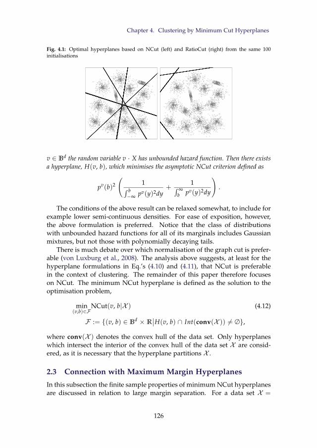
Chapter 4. Clustering by Minimum Cut Hyperplanes
Fig. 4.1: Optimal hyperplanes based on NCut (left) and RatioCut (right) from the same 100initialisations
v ∈ Bd the random variable v · X has unbounded hazard function. Then there existsa hyperplane, H(v, b), which minimises the asymptotic NCut criterion defined as
pv(b)2
(1∫ b
−∞ pv(y)2dy+
1∫ ∞b pv(y)2dy
).
The conditions of the above result can be relaxed somewhat, to include forexample lower semi-continuous densities. For ease of exposition, however,the above formulation is preferred. Notice that the class of distributionswith unbounded hazard functions for all of its marginals includes Gaussianmixtures, but not those with polynomially decaying tails.
There is much debate over which normalisation of the graph cut is prefer-able (von Luxburg et al., 2008). The analysis above suggests, at least for thehyperplane formulations in Eq.’s (4.10) and (4.11), that NCut is preferablein the context of clustering. The remainder of this paper therefore focuseson NCut. The minimum NCut hyperplane is defined as the solution to theoptimisation problem,
min(v,b)∈F
NCut(v, b|X ) (4.12)
F := (v, b) ∈ Bd × R∣∣H(v, b) ∩ Int(conv(X )) 6= ∅,
where conv(X ) denotes the convex hull of the data set. Only hyperplaneswhich intersect the interior of the convex hull of the data set X are consid-ered, as it is necessary that the hyperplane partitions X .
2.3 Connection with Maximum Margin Hyperplanes
In this subsection the finite sample properties of minimum NCut hyperplanesare discussed in relation to large margin separation. For a data set X =
126
2. Problem Formulation
x1, ..., xn in Rd, the margin of a hyperplane on X is the Euclidean distancebetween the hyperplane and X , i.e.,
marginH(v, b) := d(H(v, b), X ) = mini∈1,...,n
|v · xi − b|. (4.13)
Maximum margin hyperplane classifiers have become extremely popular overthe past few decades, owing to the success of Support Vector Machines (SVM,(Vapnik and Kotz, 1982)). SVM classifiers were introduced for supervisedclassification, and extended to semi-supervised learning via TransductiveSupport Vector Machines (TSVM, (Vapnik, 1998)). More recently the sup-port vector approach has been successfully applied to the fully unsupervisedproblem of maximum margin clustering (Xu et al., 2004; Zhang et al., 2009).The maximum margin clustering problem can be equvalently stated as iden-tifying the binary labelling of a data that will maximimise the margin of anSVM estimated using the assigned labels. Early maximum margin clusteringalgorithms used semi-definite programming formulations, which limits theirapplication to data sets of only a few hundred points (Xu et al., 2004). Theiterative Support Vector Regression approach (Zhang et al., 2009) repeatedlysolves a support vector regression problem, updating the labels assigned tothe data after each iteration. This method has shown strong performance em-pirically and has allowed the application of large margin clustering to muchlarger problems than was feasible previously.
The following lemma establishes the convergence of the minimum NCuthyperplane to the maximum margin hyperplane, as the scaling parame-ter is reduced to zero. Notice that for v ∈ Bd and for b1, b2 ∈ R s.t. X ∩H(v, b1)
+ = X ∩ H(v, b2)+ one has NCut(v, b1|X ) = NCut(v, b2|X ). As a
result there is not a unique minimum cut hyperplane. The convergence tothe maximum margin hyperplane is therefore discussed only in relation tothe normal vector. Notice that if the normal vector to the maximum marginhyperplane is known, then obtaining the maximum margin hyperplane istrivial. These two results are thus practically equivalent.
Lemma 24 Let X = x1, ..., xn be a data set in Rd. Suppose there is a unique hy-perplane intersecting conv(X ) with maximum margin, parameterised by (vm, bm) ∈Bd × R. For σ > 0 define (vσ, bσ) to be any minimiser of the optimisation prob-lem min(v,b)∈F NCut(v, b|X , σ), where there is now an explicit dependence on thescaling parameter, σ. Then,
limσ→0+
d(vσ, vm, −vm) = 0.
The above result relies on the fact that the NCut objective can be viewed asa sort of smoothing of the maximum margin clustering problem, in that forlarge values of σ the global structure of the data set defines the strength of
127
Chapter 4. Clustering by Minimum Cut Hyperplanes
the clustering solution, but as σ decreases towards zero points nearer the hy-perplane become more influential, and asymptotically it is dominated by thenearest points. Solving the minimum cut hyperplane problem repeatedly fora shrinking sequence of scaling parameters is thus strongly reminiscent of thehomotopy continuation approach to non-convex optimisation (Allgower andGeorg, 2012), in which an objective function is convolved with a sequenceof smoothing functions the last of which is the identity function. Initialis-ing each smoothed problem using the solution to the previous provides asequence of solutions which converges to a good solution to the original op-timisation problem.
The above result provides a new approach for finding large margin hy-perplanes for clustering. One of the challenges associated with maximummargin clustering is the fact that the objective is plagued with local min-ima (Zhang et al., 2009). The above approach, due to its similarity withhomotopy continuation, has the potential to mitigate this problem, and there-fore generate higher quality solutions than those based directly on supportvector methods.
3 Methodology
In the previous section, properties of hyperplane based graph cuts were in-troduced. It was established that the optimal hyperplane based on NCut isa preferable objective to that for RatioCut. This section is dedicated to op-timising NCut(v, b|X ) over (v, b) ∈ F , where X is a data set in Rd. Theoptimisation procedure proposed treats optimising over b as a subproblemto the master problem of optimising over v.
The global objective is thus formulated as,
minv∈Bd
Φ(v|X ), (4.14)
Φ(v|X ) := minb∈Int(conv(v·X ))
NCut(v, b|X ). (4.15)
Subsection 3.1 describes the optimisation procedure of the subproblem inEq. (4.15). A log-linear time method is presented, wherein the log factorarises solely from the requirement that the marginal data set, v · X , mustbe sorted. Subsection 3.2 is dedicated to the optimisation of Φ(v|X ). Thesesuffice to generate a bipartition of X , which is the main focus of this work.Extensions to multi-cluster partitions are covered briefly in subsection 3.3.
3.1 Optimal NCut of the Marginal Data Set v · XIn this subsection it is assumed that the vector v ∈ Bd is fixed, and the optimalvalue of b is to be determined based on the marginal data set, v · X . For
128

3. Methodology
brevity of notation the i-th element of the sorted marginal data set is denotedxv
i . That is, xv1 ≤ xv
2 ≤ ... ≤ xvn. Ties may be broken in an arbitrary but well
defined manner, such as via the order of indices in the original data set.Observe that for b1, b2 ∈ (xv
i , xvi+1] we have NCut(v, b1|X ) = NCut(v, b2|X )
and hence one needs only consider at most n − 1 possible values of b, cor-responding to the midpoints between consecutive distinct elements of themarginal data set. To that end, define
bi :=xv
i + xvi+1
2, i ∈ 1, ..., n − 1. (4.16)
Define CS(·) to be the cumulative sum function. That is, if w has length n,
CS(w) =
(w1,
2
∑i=1
wi, . . . ,n
∑i=1
wi
). (4.17)
Let EG be the vector of exponentials of the scaled differences between xv1 and
each element in the sorted marginal data set, i.e.,
EG :=(
exp(
xv1−xv
1σ
),exp
(xv
1−xv2
σ
),...,exp
(xv
1−xvn
σ
)). (4.18)
Then, for i≤ j,
Kσ(xvi ,xv
j )=exp
(xv
i −xvj
σ
)=
exp(
xv1−xv
jσ
)exp
(xv
1−xvi
σ
) =EGj
EGi
Therefore, the graph cut at bk is given by,
k
∑i=1
n
∑j=k+1
Kσ(xvi ,xv
j )=k
∑i=1
n
∑j=k+1
EGj
EGi=
k
∑i=1
1EGi
n
∑j=k+1
EGj
=CS(
1EG
)k(CS(EG)n−CS(EG)k).
Similarly, the sum of the first k degrees in the graph of v·X is given by,
k
∑i=1
n
∑j=1
Kσ(xvi ,xv
j )=k
∑i=1
n
∑j=i+1
EGj
EGi+
k
∑i=1
i
∑j=1
EGiEGj
=k
∑i=1
1EGi
(CS(EG)n−CS(EG)i)+k
∑i=1
EGiCS(
1EG
)i
=CS(
1EG·(CS(EG)n−CS(EG))
)k+CS
(EG ·CS
(1
EG
))k.
129
Chapter 4. Clustering by Minimum Cut Hyperplanes
The NCut for any bk can therefore be extracted from a collection of cumu-lative sum vectors. Computing these vectors has computational cost O(n),with the extraction of each NCut(v, bk|X ) costing O(1). The solution to theproblem minb NCut(v, b|X ) can therefore be computed in O(n log n) time,with the log n factor only arising in the sorting of the marginal data set, v · X .
3.2 Optimising Φ(v|X )
In this subsection the optimisation of the master problem, minv∈Bd Φ(v|X )is discussed. Notice that Φ(v|X ) may not be continuous in v, since if v · Xcontains repeated points these cannot be assigned to different elements ofthe partition, while in any neighbourhood of v there exist projections alongwhich they can be. In practice the following optimisation problem is consid-ered instead,
minv|‖v‖≥1
mink∈1,...,n−1
φk
(v‖v‖
∣∣X), (4.19)
φk(v|X ) :=k
∑i=1
n
∑j=k+1
Kσ(xvi ,xv
j )
1k∑
i=1
n∑
j=1Kσ(xv
i ,xvj )
+1
n∑
i=k+1
n∑
j=1Kσ(xv
i ,xvj )
,
(4.20)
where the computation of mink φk(v/‖v‖|X ) is described in the previoussubsection. It is straightforward to see that the above problem is practicallyequivalent to the minimisation of Φ(v|X ) in general. Notice that if v is suchthat v · X contains no repeated points, then
mink∈1,...,n−1
φk
(v‖v‖
∣∣X) = Φ(
v‖v‖
∣∣X) .
If the full dimensional data set, X , contains no repeated points and for allv 6= 0 one has Int(conv(v · X )) 6= ∅, then this occurs on an open and denseset in Rd. For those v s.t. v · X does contain repeated points, evaluatingmink φk(v/‖v‖|X ) is the same as for Φ(v/‖v‖|X ), except that some par-titions which separate equal elements of v · X are permitted. Therefore,mink φk(v/‖v‖|X ) ≤ Φ(v/‖v‖|X ) and hence for all v 6= 0 one has
liminfw→vΦ(w/‖w‖|X ) = mink
φk(v/‖v‖|X ).
The objective in (4.19) benefits from being continuous, and is in fact Lips-chitz continuous over the set v ∈ Rd|‖v‖ ≥ 1, as discussed below. The ob-jective is therefore differentiable almost everywhere, and so gradient based
130
3. Methodology
methods can be used to find local optima. In general the objective is notdifferentiable at points where mink φk(v/‖v‖
∣∣X ) is satisfied by multiple in-dices k, and where the order statistics corresponding to the minimum co-incide. Considerable work has been done on optimising such non-smoothobjectives, however it has been observed that the BFGS (Broyden-Fletcher-Goldfarb-Shanno) algorithm tends to perform well on many non-smoothfunctions (Lewis and Overton, 2013). Indeed, applying this method to op-timising mink φk(v/‖v‖
∣∣X ) did not fail to find a local optimum in any exam-ples considered for this work.
The Lipschitz continuity of the objective mink φk(v/‖v‖∣∣X ) is now briefly
discussed. Consider v ∈ Rd \ 0 and u ∈ Rd, u 6= −v. The order statisticsof the marginal data set, v · X , are Lipschitz continuous as functions of v andso ∃L > 0 s.t. for any i, j ∈ 1, ..., n,∣∣∣(xv
i − xvj ) − (xv+u
i − xv+uj )
∣∣∣ ≤ L‖u‖.
It is therefore straightforward to show that,∣∣∣∣∣ xvi − xv
j
‖v‖ −xv+u
i − xv+uj
‖v + u‖
∣∣∣∣∣ ≤ (L + Diam(X ))‖u‖‖v‖
⇒∣∣∣∣∣exp
(−|xv
i − xvj |
‖v‖σ
)− exp
(−|xv+u
i − xv+uj |
‖v + u‖σ
)∣∣∣∣∣ ≤ (L + Diam(X ))‖u‖‖v‖σ ,
since exp(−x) has Lipschitz constant 1. From this it can be shown that for‖u‖ ≤ 1, ∃H > 0 s.t. each φk satisfies∣∣∣∣φk
(v‖v‖
∣∣X) − φk
(v + u‖v + u‖
∣∣X)∣∣∣∣ ≤ H‖u‖‖v‖ ,
and hence the objective mink φk(v/‖v‖∣∣X ) is Lipschitz continuous in v over
the set v ∈ Rd∣∣‖v‖ ≥ 1.
In what follows, derivations of the gradient of mink φk(v/‖v‖∣∣X ) are pre-
sented for those v where the minimum is unique, and where order statisticscorresponding to the minimum do not coincide. The chain rule decomposi-tion below is used.
Dvφk
(v‖v‖
∣∣X)=D v‖v‖ ·X
NCut(xv‖v‖1 ,...,x
v‖v‖k ,x
v‖v‖k+1,...,x
v‖v‖n )Dv
v‖v‖ ·X ,
(4.21)
where D·· is the differential operator. First observe that,
Dvv‖v‖ · X =
1‖v‖X −
1‖v‖3X (vv>),
131
Chapter 4. Clustering by Minimum Cut Hyperplanes
where here X is treated as a matrix in Rn×d in which the i-th row correspondsto xi. Therefore,
(Dvv‖v‖ · X ) · v = 0
⇒∥∥∥∥v − δDvφk
(v‖v‖ |X
)∥∥∥∥ ≥ ‖v‖for any δ > 0. This means that iterations in a simple gradient descent methodhave increasing norm. We have also observed that this behaviour transfersto the BFGS algorithm, even though the approximate Hessian is included inthe search direction. Thus the constraint ‖v‖ ≥ 1 in the optimisation (4.19) isinactive provided the initial solution has norm at least 1. The optimisationcan therefore be treated as unconstrained in practice.
What remains is to address the first component in the chain rule decom-position (4.21). For ease of notation, let xv
i = xv/‖v‖i . Define,
E :=
(exp
(xv
1−xvk
σ
),exp
(xv
2−xvk
σ
),. . .,exp
(xv
n−xvk
σ
)).
Then for l≤k, and using a similar derivation to those in Subsection 3.1, onehas the following,
∂
∂xvl
k
∑i=1
n
∑j=k+1
Kσ(xvi ,xv
j )=1σ
El
(CS(
1E
)n−CS
(1E
)k
).
In addition,
∂
∂xvl
k
∑i=1
n
∑j=1
Kσ(xvi ,xv
j )=−2σ
CS(E)l−1El
+2σ
El
(CS(
1E
)k−CS
(1E
)l
)+
1σ
El
(CS(
1E
)n−CS
(1E
)k
).
If l=1 then the first term above is 0. In a similar way one finds,
∂
∂xvl
n
∑i=k+1
n
∑j=1
Kσ(xvi ,xv
j )=1σ
El
(CS(
1E
)n−CS
(1E
)k
),
132
3. Methodology
and for l>k, the following,
∂
∂xvl
k
∑i=1
n
∑j=k+1
Kσ(xvi ,xv
j )=−1σ
CS(E)kEl
∂
∂xvl
k
∑i=1
n
∑j=1
Kσ(xvi ,xv
j )=−1σ
CS(E)kEl
∂
∂xvl
n
∑i=k+1
n
∑j=1
Kσ(xvi ,xv
j )=2σ
El
(CS(
1E
)n−CS
(1E
)l
)
− 2σ
CS(E)l−1−CS(E)kEl
− 1σ
CS(E)kEl
.
The partial derivative of NCut(xv1 ,...,xv
k,xvk+1,...,xv
n) with respect to thel-th element of v
‖v‖ ·X is given by
∂
∂xvl
k
∑i=1
n
∑j=k+1
Kσ(xvi ,xv
j )
1k∑
i=1
n∑
j=1Kσ(xv
i ,xvj )
+1
n∑
i=k+1
n∑
j=1Kσ(xv
i ,xvj )
−k
∑i=1
n
∑j=k+1
Kσ(xvi ,xv
j )
∂
∂xvl
k∑
i=1
n∑
j=1Kσ(xv
i ,xvj )(
k∑
i=1
n∑
j=1Kσ(xv
i ,xvj )
)2 +
∂∂xv
l
n∑
i=k+1
n∑
j=1Kσ(xv
i ,xvj )(
n∑
i=k+1
n∑
j=1Kσ(xv
i ,xvj )
)2
.
Therefore the collection of all partial derivatives can be computed in O(n)time, since each can be extracted in constant time from a collection of cumu-lative sum vectors.
3.3 Beyond Bi-partitioning
So far methodology for inducing a bipartition of a data set X using the mini-mum cut hyperplane has been discussed. This divisive procedure can be ap-plied recursively to (subsets of) the data set to generate a binary partitioningtree. An indexing policy is required which assigns an ordering to the leavesof the tree, dictating which should be further partitioned at the next iteration.This process is repeated until a predetermined number of leaves results, andthe data assigned to each leaf are interpreted as clusters. Pseudocode for ageneric divisive clustering algorithm is given in Algorithm 1.
Two methods are considered. The first uses the procedure in Subsec-tions 3.1 and 3.2 to induce bipartitions, and selects the leaf which has the
133
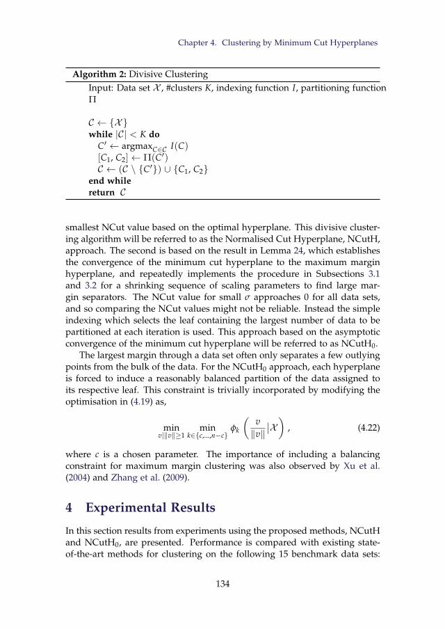
Chapter 4. Clustering by Minimum Cut Hyperplanes
Algorithm 2: Divisive ClusteringInput: Data set X , #clusters K, indexing function I, partitioning functionΠ
C ← Xwhile |C| < K do
C′ ← argmaxC∈C I(C)[C1, C2]← Π(C′)C ← (C \ C′) ∪ C1, C2
end whilereturn C
smallest NCut value based on the optimal hyperplane. This divisive cluster-ing algorithm will be referred to as the Normalised Cut Hyperplane, NCutH,approach. The second is based on the result in Lemma 24, which establishesthe convergence of the minimum cut hyperplane to the maximum marginhyperplane, and repeatedly implements the procedure in Subsections 3.1and 3.2 for a shrinking sequence of scaling parameters to find large mar-gin separators. The NCut value for small σ approaches 0 for all data sets,and so comparing the NCut values might not be reliable. Instead the simpleindexing which selects the leaf containing the largest number of data to bepartitioned at each iteration is used. This approach based on the asymptoticconvergence of the minimum cut hyperplane will be referred to as NCutH0.
The largest margin through a data set often only separates a few outlyingpoints from the bulk of the data. For the NCutH0 approach, each hyperplaneis forced to induce a reasonably balanced partition of the data assigned toits respective leaf. This constraint is trivially incorporated by modifying theoptimisation in (4.19) as,
minv|‖v‖≥1
mink∈c,...,n−c
φk
(v‖v‖
∣∣X) , (4.22)
where c is a chosen parameter. The importance of including a balancingconstraint for maximum margin clustering was also observed by Xu et al.(2004) and Zhang et al. (2009).
4 Experimental Results
In this section results from experiments using the proposed methods, NCutHand NCutH0, are presented. Performance is compared with existing state-of-the-art methods for clustering on the following 15 benchmark data sets:
134
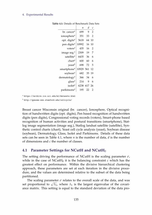
4. Experimental Results
Table 4.1: Details of Benchmark Data Sets
n d c
br. cancera 699 9 2
ionospherea 351 33 2
opt. digitsa 5618 64 10
pen digitsa 10992 16 10
votersa 435 16 2
image seg.a 2309 19 7
satellitea 6435 36 6
charta 600 60 6
yeastb 698 72 5
smartphonea 10929 561 12
soybeana 682 35 19
dermatologya 366 34 6
glassa 214 9 6
isoleta 6238 617 26
parkinsonsa 195 22 2
a https://archive.ics.uci.edu/ml/datasets.htmlb http://genome-www.stanford.edu/cellcycle/
Breast cancer Wisconsin original (br. cancer), Ionosphere, Optical recogni-tion of handwritten digits (opt. digits), Pen based recognition of handwrittendigits (pen digits), Congressional voting records (voters), Smart-phone basedrecognition of human activities and postural transitions (smartphone), Stat-log image segmentation (image seg.), Statlog landsat satellite (satellite), Syn-thetic control charts (chart), Yeast cell cycle analysis (yeast), Soybean disease(soybean), Dermatology, Glass, Isolet and Parkinsons. Details of these datasets can be seen in Table 4.1, where n is the number of data, d is the numberof dimensions and c the number of classes.
4.1 Parameter Settings for NCutH and NCutH0
The setting driving the performance of NCutH is the scaling parameter σ,while in the case of NCutH0 it is the balancing constraint c which has thegreatest effect on performance. Within the divisive hierarchical clusteringapproach, these parameters are set at each iteration in the divisive proce-dure, and the values are determined relative to the subset of the data beingpartitioned.
The scaling parameter σ relates to the overall scale of the data, and wasset proportional to
√λ1, where λ1 is the largest eigenvalue of the covari-
ance matrix. This setting is equal to the standard deviation of the data pro-
135
Chapter 4. Clustering by Minimum Cut Hyperplanes
jected along the first principal component. The analysis in Section 2 suggestssetting σ ∝ n−1/(4+ε) for some ε > 0, and ε is set to 1 for the experimentsherein. To determine an appropriate constant of proportionality, a simplesimulation study using Gaussian mixtures was performed. Simulations areextremely useful for determining appropriate values of tuning parameters asthe true class labels are known, and so the clustering performance can bedetermined reliably. In this study Gaussian mixtures containing between 2and 10 components, and in 5, 10 and 50 dimensions were simulated. Thedata arising from each component were assigned the same class label andthese were compared with the cluster assignments made by NCutH for valuesof σ in σ0, 5σ0, 10σ0, 50σ0, 100σ0, 200σ0 where σ0 =
√λ1n−1/5. Aside from
σ = σ0, the mean performance for all other values of σ was approximatelythe same accross the range of dimensions and number of clusters. Howeverfor σ = 50σ0 and σ = 100σ0 the variability of performance was slightly lower.For the experiments presented below the value σ = 100σ0 was used, but it isapparent from this study that performance is robust over a range of values.One observation made possible by this study is that the cluster sizes tend tobe more balanced for larger values of σ, although this is not guaranteed.
The value of the balancing constraint parameter c was set to n/5, whichis equivalent to the setting used by Zhang et al. (2009) for maximum marginclustering when the cluster sizes are not balanced. Since this parameter offersa direct interpretation in terms of the minimum cluster size, prior informa-tion about the sizes of clusters can be incorprated into the method. To findlarge margin hyperplanes using the NCutH0 approach, the scaling parame-ter was initialised at 100σ0, as above, and subsequently decreased by a factorof 5 at each iteration. This was repeated until convergence of the optimalhyperplane.
In addition, since the minimisation of NCut(v, b) is non-convex, the ini-tialisation of v also plays a significant role. For initialisation of the vector v,the first principal component of the data was used. It is intuitively the casethat directions with high data variability are likely to admit high quality hy-perplanes for clustering, and so are likely to present promising initialisationsfor the proposed optimisation method.
4.2 Clustering Performance
The following benchmark algorithms were chosen for comparison with NCutHand NCutH0:
1. K-means using the default implementation in R. Results from the bestsolution based on the K-means objective from 10 initialisations are re-ported.
2. Bisecting K-means (Bis.K-m) (Steinbach et al., 2000). The bisecting ver-
136
4. Experimental Results
sion of K-means offers a useful comparison with the proposed methoddue to the similar model structure.
3. Normalised Spectral Clustering (SCn). Due to the high computationtime required, when the number of data exceeds 1000 the approxima-tion method given by Yan et al. (2009) was used.1 A range of scalingparameters was used, and the highest performance is reported. Spectralclustering is a highly influential approach to clustering, and is based onthe same normalised graph cut objective as the proposed method.
4. Iterative Support Vector Regression (iSVR). A state-of-the-art methodfor maximum margin clustering (Zhang et al., 2009).2 To generate mul-tiple clusters the same hierarchical method as for NCutH0 is used, split-ting the largest remaining cluster at each iteration.
5. Density enhanced principal direction divisive partitioning (dePDDP)(Tasoulis et al., 2010). An improvement of one of the earliest divisive hi-erarchical clustering algorithms using hypeprlanes, Principal DirectionDivisive Partitioning. To make the comparison fair the correct numberof clusters is supplied to the algorithm.
The algorithms are compared based on cluster Purity (Zhao and Karypis,2004) and V-Measure (Rosenberg and Hirschberg, 2007). Both measures com-pare the true classes in the data with the cluster assignments made by analgorithm. They take values in [0, 1] with higher values indicating superiorperformance. Purity is defined as the weighted average of the largest pro-portion of each cluster which is represented by a single class. V-Measure isdefined as the harmonic mean of homogeneity and completeness. Homogeneitymeasures the conditional entropy of the class distribution within each cluster.Completeness is symmetric to homogeneity, and measures the conditionalentropy of the cluster distribution within each class. V-Measure thereforecaptures both the extent to which each cluster can be associated with a sin-gle class, but also penalises cluster assignments which divide single classesbetween multiple clusters.
Tables 4.2 and 4.3 report the Purity and V-Measure respectively. The high-est performance in each case is highlighted in bold, while - indicates that aclustering result could not be obtained in reasonable time. It is clear that nomethod is uniformly superior to all others, which is due to the vastly differ-ent natures of the data sets in terms of size, dimension, number and shape ofclusters. It is also clear that the problems of clustering the various data setsdiffer in difficulty. Both NCutH and NCutH0 obtained the highest perfor-mance at least as often as any of the competing methods, and in the case of
1The implementation available at http://www.math.umassd.edu/˜dyan/fasp.html is em-ployed
2Thanks to Dr. Kai Zhang for providing code for this method.
137
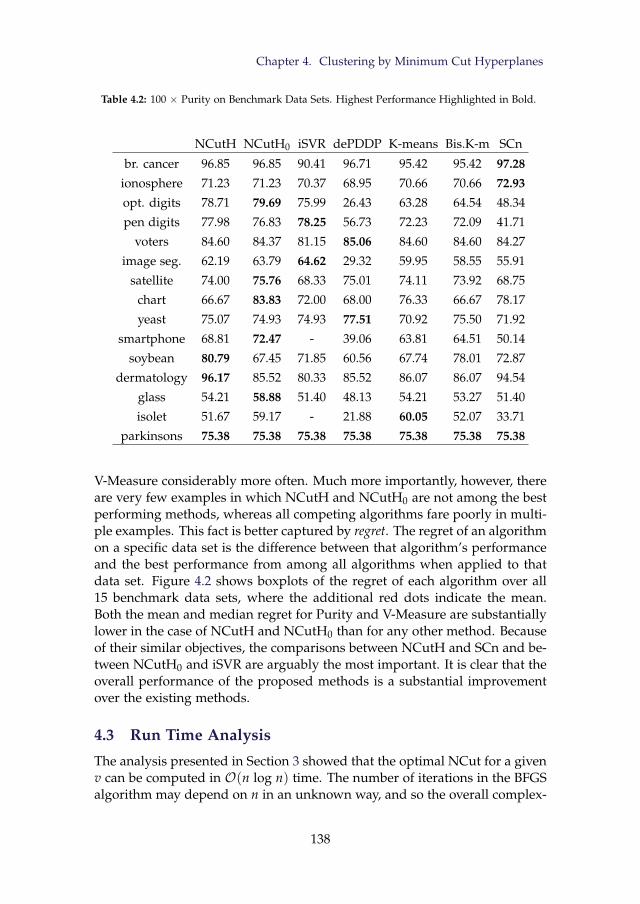
Chapter 4. Clustering by Minimum Cut Hyperplanes
Table 4.2: 100 × Purity on Benchmark Data Sets. Highest Performance Highlighted in Bold.
NCutH NCutH0 iSVR dePDDP K-means Bis.K-m SCn
br. cancer 96.85 96.85 90.41 96.71 95.42 95.42 97.28ionosphere 71.23 71.23 70.37 68.95 70.66 70.66 72.93opt. digits 78.71 79.69 75.99 26.43 63.28 64.54 48.34
pen digits 77.98 76.83 78.25 56.73 72.23 72.09 41.71
voters 84.60 84.37 81.15 85.06 84.60 84.60 84.27
image seg. 62.19 63.79 64.62 29.32 59.95 58.55 55.91
satellite 74.00 75.76 68.33 75.01 74.11 73.92 68.75
chart 66.67 83.83 72.00 68.00 76.33 66.67 78.17
yeast 75.07 74.93 74.93 77.51 70.92 75.50 71.92
smartphone 68.81 72.47 - 39.06 63.81 64.51 50.14
soybean 80.79 67.45 71.85 60.56 67.74 78.01 72.87
dermatology 96.17 85.52 80.33 85.52 86.07 86.07 94.54
glass 54.21 58.88 51.40 48.13 54.21 53.27 51.40
isolet 51.67 59.17 - 21.88 60.05 52.07 33.71
parkinsons 75.38 75.38 75.38 75.38 75.38 75.38 75.38
V-Measure considerably more often. Much more importantly, however, thereare very few examples in which NCutH and NCutH0 are not among the bestperforming methods, whereas all competing algorithms fare poorly in multi-ple examples. This fact is better captured by regret. The regret of an algorithmon a specific data set is the difference between that algorithm’s performanceand the best performance from among all algorithms when applied to thatdata set. Figure 4.2 shows boxplots of the regret of each algorithm over all15 benchmark data sets, where the additional red dots indicate the mean.Both the mean and median regret for Purity and V-Measure are substantiallylower in the case of NCutH and NCutH0 than for any other method. Becauseof their similar objectives, the comparisons between NCutH and SCn and be-tween NCutH0 and iSVR are arguably the most important. It is clear that theoverall performance of the proposed methods is a substantial improvementover the existing methods.
4.3 Run Time Analysis
The analysis presented in Section 3 showed that the optimal NCut for a givenv can be computed in O(n log n) time. The number of iterations in the BFGSalgorithm may depend on n in an unknown way, and so the overall complex-
138
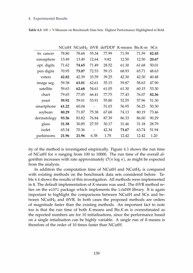
4. Experimental Results
Table 4.3: 100 × V-Measure on Benchmark Data Sets. Highest Performance Highlighted in Bold.
NCutH NCutH0 iSVR dePDDP K-means Bis.K-m SCn
br. cancer 78.80 78.68 55.34 77.99 71.59 71.59 82.45ionosphere 13.49 13.49 12.64 9.82 12.50 12.50 20.67opt. digits 71.62 74.65 71.49 28.52 61.30 61.68 50.01
pen digits 70.95 73.07 72.53 59.15 68.93 65.71 48.63
voters 42.82 42.39 33.59 39.25 42.30 42.30 40.48
image seg. 59.38 63.81 62.61 35.15 59.87 58.63 47.90
satellite 59.63 62.68 54.61 61.05 61.30 60.15 53.30
chart 79.65 77.05 66.41 77.75 77.43 76.07 82.36yeast 59.92 59.01 53.91 55.80 52.55 57.96 51.30
smartphone 61.22 60.04 - 51.03 56.95 56.25 50.30
soybean 80.29 71.87 75.38 67.68 74.13 80.19 73.46
dermatology 93.56 83.82 76.84 87.39 86.33 86.00 90.29
glass 31.58 30.85 27.55 30.17 31.46 31.18 28.79
isolet 65.34 70.36 - 42.34 71.67 63.74 51.94
parkinsons 21.96 21.96 6.38 1.78 12.42 12.42 1.20
ity of the method is investigated empirically. Figure 4.3 shows the run timeof NCutH for n ranging from 100 to 10000. The run time of the overall al-gorithm increases with rate approximately O(n log n), as might be expectedfrom the analysis.
In addition the computation time of NCutH and NCutH0 is comparedwith existing methods on the benchmark data sets considered before. Ta-ble 4.4 shows the results of this investigation. All methods were implementedin R. The default implementation of K-means was used. The iSVR method re-lies on the e1071 package which implements the libSVM library. It is againimportant to highlight the comparisons between NCutH and SCn and be-tween NCutH0 and iSVR. In both cases the proposed methods are ordersof magnitude faster than the existing methods. An important fact to notetoo is that the run time of both K-means and Bis.K-m is overestimated asthe reported numbers are for 10 initialisations, since the performance basedon a single intialisation can be highly variable. A single run of K-means istherefore of the order of 10 times faster than NCutH.
139
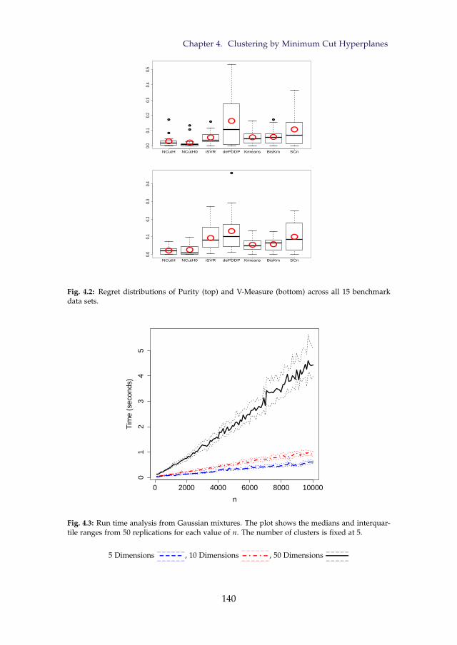
Chapter 4. Clustering by Minimum Cut Hyperplanes
NCutH NCutH0 iSVR dePDDP Kmeans BisKm SCn0.
00.
10.
20.
30.
40.
5
NCutH NCutH0 iSVR dePDDP Kmeans BisKm SCn
0.0
0.1
0.2
0.3
0.4
Fig. 4.2: Regret distributions of Purity (top) and V-Measure (bottom) across all 15 benchmarkdata sets.
0 2000 4000 6000 8000 10000
01
23
45
n
Tim
e (s
econ
ds)
Fig. 4.3: Run time analysis from Gaussian mixtures. The plot shows the medians and interquar-tile ranges from 50 replications for each value of n. The number of clusters is fixed at 5.
5 Dimensions −−−−−−– – – –– – – –– – – –−−−−−−
, 10 Dimensions−−−−−−– · – · –– · – · –– · – · –−−−−−−
, 50 Dimensions −−−−−—————————−−−−−
140

5. Conclusion
Table 4.4: Run Time on Benchmark Data Sets (in Seconds)
NCutH NCutH0 iSVR dePDDP K-means Bis.K-m SCn
br. cancer 0.01 0.23 1.81 0.01 0.05 0.05 0.67
ionosphere 0.01 0.16 2.47 0.02 0.03 0.05 0.20
opt. digits 4.40 12.01 496.14 0.19 1.97 4.04 28.37
pen digits 1.55 6.37 347.77 0.12 0.79 2.35 24.29
voters 0.02 0.16 1.09 0.01 0.03 0.03 0.27
image seg. 0.39 1.22 18.19 0.06 0.17 0.52 6.15
satellite 0.81 3.26 203.30 0.11 0.95 2.54 21.67
chart 0.20 0.78 14.32 0.12 0.11 0.40 1.61
yeast 0.31 1.06 21.82 0.06 0.19 0.55 2.34
smartphone 81.04 217.38 - 14.71 82.29 103.36 1915.10
soybean 0.47 1.48 12.21 0.15 0.08 0.29 0.19
dermatology 0.13 0.56 1.17 0.06 0.03 0.14 0.31
glass 0.06 0.31 0.32 0.02 0.00 0.03 0.08
isolet 80.86 220.19 - 16.43 54.06 77.95 1511.53
parkinsons 0.01 0.10 0.39 0.01 0.01 0.01 0.05
5 Conclusion
This paper presents a novel hyperplane based method for clustering. Theoptimal hyperplane is that which minimises the normalised graph cut mea-sured across it. The asymptotic properties for an incrceasing sample assumedto arise from an underlying probability distribution are established, showingthat the minimum NCut hyperplane tends to have low density along it, aswell as separate modes of the underlying probability density. Both of theseare key features in the context of data clustering. In the finite sample case,the minimum cut hyperplane is asymptotically connected with the maximummargin hyperplane through the data, as the scaling parameter decreases tozero. Applying the proposed method for a shrinking sequence of scalingparameters also therefore provides a new method for finding large marginseparators. Exploiting the trivial factorisation of the exponential function al-lows for the derivation of a linear time method for extracting the optimalnormalised cut of a sorted univariate marginal data set. The overall algo-rithm has empirical time complexity which is log-linear in the number ofdata, allowing for the application to larger data sets than is generally true ofgraph based partitioning methods.
In experiments on a large collection of benchmark data sets the proposedmethod showed superior performance to a collection of influential clustering
141
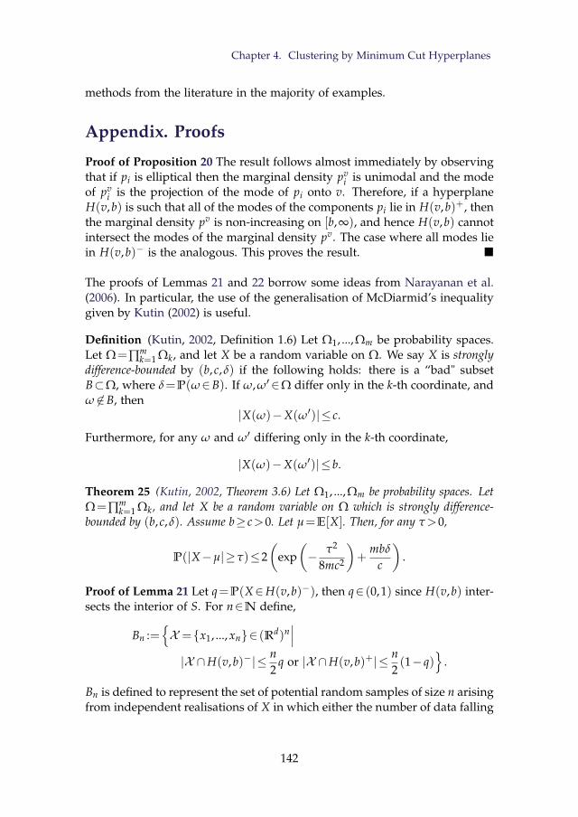
Chapter 4. Clustering by Minimum Cut Hyperplanes
methods from the literature in the majority of examples.
Appendix. Proofs
Proof of Proposition 20 The result follows almost immediately by observingthat if pi is elliptical then the marginal density pv
i is unimodal and the modeof pv
i is the projection of the mode of pi onto v. Therefore, if a hyperplaneH(v,b) is such that all of the modes of the components pi lie in H(v,b)+, thenthe marginal density pv is non-increasing on [b,∞), and hence H(v,b) cannotintersect the modes of the marginal density pv. The case where all modes liein H(v,b)− is the analogous. This proves the result.
The proofs of Lemmas 21 and 22 borrow some ideas from Narayanan et al.(2006). In particular, the use of the generalisation of McDiarmid’s inequalitygiven by Kutin (2002) is useful.
Definition (Kutin, 2002, Definition 1.6) Let Ω1, ...,Ωm be probability spaces.Let Ω=∏m
k=1 Ωk, and let X be a random variable on Ω. We say X is stronglydifference-bounded by (b, c,δ) if the following holds: there is a “bad" subsetB⊂Ω, where δ=P(ω∈B). If ω,ω′∈Ω differ only in the k-th coordinate, andω 6∈B, then
|X(ω)−X(ω′)|≤ c.
Furthermore, for any ω and ω′ differing only in the k-th coordinate,
|X(ω)−X(ω′)|≤b.
Theorem 25 (Kutin, 2002, Theorem 3.6) Let Ω1, ...,Ωm be probability spaces. LetΩ=∏m
k=1 Ωk, and let X be a random variable on Ω which is strongly difference-bounded by (b, c,δ). Assume b≥ c>0. Let µ=E[X]. Then, for any τ>0,
P(|X−µ|≥τ)≤2(
exp(− τ2
8mc2
)+
mbδ
c
).
Proof of Lemma 21 Let q=P(X∈H(v,b)−), then q∈ (0,1) since H(v,b) inter-sects the interior of S. For n∈N define,
Bn :=X =x1, ..., xn∈ (Rd)n
∣∣∣|X ∩H(v,b)−|≤ n
2q or |X ∩H(v,b)+|≤ n
2(1−q)
.
Bn is defined to represent the set of potential random samples of size n arisingfrom independent realisations of X in which either the number of data falling
142

5. Conclusion
in H(v,b)+ or the number falling in H(v,b)− is less than or equal to half theexpected number. Using Hoeffding’s inequality one can show that,
P(X ∈Bn)≤exp
(−2
(nq− n2 q)2
n
)
+exp
(−2
(n(1−q)− n2 (1−q))2
n
).
Now, for X =x1, ..., xn 6∈Bn, define X ′ to be X except one of the elements isreplaced with another independent realisation of X. Define C=X ∩H(v,b)−,C′=X ′∩H(v,b)−. Then,∣∣∣∣∣∑x∈C ∑y∈X\C Kv
σ(x,y)|C|(n−|C|) −
∑x∈C′ ∑y∈X ′\C′ Kvσ(x,y)
|C′|(n−|C′|)
∣∣∣∣∣≤max
1|C|−1
,1
n−|C|−1
.
Since X 6∈Bn we know that |C|> n2 q and n−|C|> n
2 (1−q), and hence thisright hand side can be replaced with 2
nminq,1−q .Now, if X and X ′ are again defined as above except X is allowed to lie in
Bn, then we instead have∣∣∣∣∣∑x∈C ∑y∈X\C Kvσ(x,y)
|C|(n−|C|) −∑x∈C′ ∑y∈X ′\C′ Kv
σ(x,y)|C′|(n−|C′|)
∣∣∣∣∣≤1.
The random variable ξ := 1nσ2 RatioCut(v,b|X ) is therefore strongly difference
bounded by, (1σ2 ,
2nminq,1−qσ2 ,P(X ∈Bn)
).
By the generalisation of McDiarmid’s inequality we thus have,
P (|ξ−E[ξ]|>γ)≤2exp(−γ2nminq,1−q2σ4
32
)+n2 minq,1−qP(X ∈Bn).
Now, let Y, Z be random variables with the same distribution as v ·X. Thenwe can write,
E[ξ]=E
[1σ2 Kσ(Z,Y)
∣∣Z<b,Y≥b]
.
Therefore,
E[ξ]=∫
_−∞b∫ ∞
b
1σ2 Kσ(z,y)
pv(z)P(v ·X<b)
pv(y)P(v ·X≥b)
dydz
=∫ b
−∞
∫ ∞
b
1σ2 exp
(z−y
σ
)pv(z)
P(v ·X<b)pv(y)
P(v ·X≥b)dydz
=∫ b
−∞
1σ
exp(
z−bσ
)pv(z)
P(v ·X<b)
∫ ∞
b
1σ
exp(
b−yσ
)pv(y)
P(v ·X≥b)dydz.
143

Chapter 4. Clustering by Minimum Cut Hyperplanes
Now, the quantity∫ b−∞
1σ exp
(z−b
σ
)pv(z)
P(v·X<b)dz is the expected value of a ker-nel estimate of the density of the random variable v ·X truncated above atb evaluated at the point b, and using a Laplace kernel with the reflectionmethod at the boundary. Therefore,∫ b
−∞
1σ
exp(
z−bσ
)pv(z)
P(v ·X<b)dz=
pv(b)P(v ·X<b)
+O(σ).
Similarly, ∫ ∞
b
1σ
exp(
b−yσ
)pv(y)
P(v ·X≥b)dy=
pv(b)P(v ·X≥b)
+O(σ).
Therefore,
E[ξ]=pv(b)2
P(v ·X<b)P(v ·X≥b)+O(σ).
In all, there exist D1, D2>0 s.t. for large n and with probability at least1−D1 exp
(−γ2σ4n
)we have,
|ξ−E[ξ]|≤γ and∣∣∣∣ pv(b)P(v ·X<b)P(v ·X≥b)
−E[ξ]
∣∣∣∣≤D2σ.
Setting γ∈O(σε/2) and allowing σ→0 appropriately as n→∞ therefore givesthe result. Proof of Lemma 22 Let X be a sample of realisations of X of size n. Definethe following,
η−=1
2σ
∑x∈X∩H(v,b)− ∑y∈X Kvσ(x,y)
|X ∩H(v,b)−|(n−1)
=1
2σ
∑x∈X∩H(v,b)− ∑y∈X ,y 6=x Kvσ(x,y)
|X ∩H(v,b)−|(n−1)+
12σ(n−1)
η+=1
2σ
∑x∈X∩H(v,b)+ ∑y∈X Kvσ(x,y)
|X ∩H(v,b)+|(n−1)
=1
2σ
∑x∈X∩H(v,b)+ ∑y∈X ,y 6=x Kvσ(x,y)
|X ∩H(v,b)+|(n−1)+
12σ(n−1)
,
where we adopt the convention 00 =0. Similar to the previous proof it can be
shown that η− and η+ are strongly difference bounded by ( 12σ , 1
nminq,1−qσ ,P(X ∈Bn)), with q and Bn defined as before. Thus for γ>0 both P(|η−−E[η−]|>γ) and P(|η+−E[η+]|>γ) are bounded above by
2exp(−γ2nminq,1−q2σ2
8
)+n2 minq,1−qP(X ∈Bn).
144

5. Conclusion
Now, again if we consider random variables Y, Z with the same distribu-tion as v ·X, then we can write
E[η−]=E
[1
2σKσ(Y, Z)|Y<b, Z 6=Y
]+
12σ(n−1)
E[η+]=E
[1
2σKσ(Y, Z)|Y≥b, Z 6=Y
]+
12σ(n−1)
.
Thus,
E[η−]=∫ b
−∞
∫ ∞
−∞
12σ
Kσ(y,z)pv(y)
P(v ·X<b)pv(z)dzdy
+1
2σ(n−1)
=1q
∫ b
−∞pv(y)
∫ ∞
−∞
12σ
exp(−|y− z|
σ
)pv(z)dzdy
+1
2σ(n−1),
where∫ ∞−∞
12σ exp
(− |y−z|
σ
)pv(z)dz is the expected value of a kernel estimate
of the density of pv at y using the Laplace kernel. Therefore,
E[η−]=1q
∫ b
−∞pv(y)2dy+O(σ+(σn)−1).
Similarly,
E[η+]=1
1−q
∫ ∞
bpv(y)2dy+O(σ+(σn)−1).
With ξ defined as before, we therefore have
E[ξ]
(1−q
E[η−]+
qE[η+]
)= pv(b)2
(1∫ b
−∞ pv(x)2dx+
1∫ ∞b pv(x)2dx
)+O(σ+(σn)−1).
145

Chapter 4. Clustering by Minimum Cut Hyperplanes
Now consider the following,
P
∣∣∣∣∣∣∣ξ(1−q)
η−− 2
σ
∑x∈X∩H(v,b)−
∑y∈X∩H(v,b)+
Kvσ(x,y)
∑x∈X∩H(v,b)−
∑y∈X
Kvσ(x,y)
∣∣∣∣∣∣∣>γ
=P
2σ
∑x∈X∩H(v,b)−
∑y∈X∩H(v,b)+
Kvσ(x,y)
∑x∈X∩H(v,b)−
∑y∈X
Kvσ(x,y)
∣∣∣∣ (n−1)(1−q)|X ∩H(v,b)+| −1
∣∣∣∣>γ
≤P
(2σ
∣∣∣∣ (n−1)(1−q)|X ∩H(v,b)+| −1
∣∣∣∣>γ∣∣|X ∩H(v,b)−|≥1
)≤exp
(−2n(1−q)2
(σγ/2
1+σγ/2
)2)+exp
(−2
(1−q)2
n
(nσγ/2−11−σγ/2
)2)
using, as before, tail bounds for the binomial distribution. A similar inequal-ity holds for ξq
η+.
Putting this all together, and setting γ=σε/2 and allowing σ→0 as n→∞s.t. nσ4+ε→∞, we have the following. There exist constants D1,D2,D3,D4,D5>0 s.t. for large n the following hold,
P(|ξ−E[ξ]|<γ)≥1−D1exp(−γ2σ4n
)P(|η−−E[η−]|<γ)≥1−D2exp
(−γ2σ2n
)P(|η+−E[η+]|<γ)≥1−D3exp
(−γ2σ2n
)P
∣∣∣∣∣∣∣ξ(1−q)
η−− 2
σ
∑x∈X∩H(v,b)−
∑y∈X∩H(v,b)+
Kvσ(x,y)
∑x∈X∩H(v,b)−
∑y∈X
Kvσ(x,y)
∣∣∣∣∣∣∣<γ
≥1−D4exp(−nσ2γ2
)
P
∣∣∣∣∣∣∣
ξqη+− 2
σ
∑x∈X∩H(v,b)−
∑y∈X∩H(v,b)+
Kvσ(x,y)
∑x∈X∩H(v,b)+
∑y∈X
Kvσ(x,y)
∣∣∣∣∣∣∣<γ
≥1−D5exp(−nσ2γ2
).
Therefore, there exist constants E1,E2>0 s.t. with probability at least 1−
146

5. Conclusion
E1exp(−γ2σ4n) we have∣∣∣∣∣∣∣∣∣∣2σ ∑
x∈X∩H(v,b)−
y∈X∩H(v,b)+
Kvσ(x,y)
1∑
x∈X∩H(v,b)−y∈X
Kvσ(x,y)
+1
∑x∈X∩H(v,b)+
y∈X
Kvσ(x,y)
−E[ξ]
(1−q
E[η−]+
qE[η+]
)∣∣∣∣∣∣∣∣∣∣<γE2.
Combining this with the fact that
E[ξ]
(1−q
E[η−]+
qE[η+]
)=pv(b)2
(1∫ b
−∞ pv(x)2dx+
1∫ ∞b pv(x)2dx
)+O(σ+(σn)−1),
gives the result.
The following technical result is useful for proving Proposition 23
Proposition 26 Let Y be a univariate random variable with distribution F, densityf and support S. Assume that f is continuous and has finitely many modes. Then∃z<supS s.t.,
f (x)∫ ∞x f (y)2dy
≥ 11−F(x)
,
for all x∈[z,supS).
Proof Since f is continuous and has finitely many modes ∃z∈ Int(S) s.t. f isnon-increasing on [z,supS). For x∈[z,supS), and integrating by parts, con-sider ∫ ∞
xf (y)2dy=
∫ ∞
xf (y)dF(y)
=[F(y) f (y)]∞x −∫ ∞
xF(y)d f (y)
≤[F(y) f (y)]∞x −∫ ∞
xd f (y)
=−[ f (y)(1−F(y))]∞x= f (x)(1−F(x)).
A simple rearranging provides the result.
147
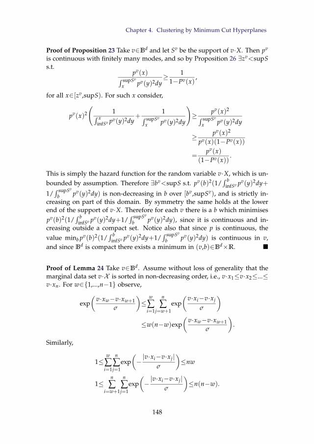
Chapter 4. Clustering by Minimum Cut Hyperplanes
Proof of Proposition 23 Take v∈Bd and let Sv be the support of v·X. Then pv
is continuous with finitely many modes, and so by Proposition 26 ∃zv<supSs.t.
pv(x)∫ supSv
x pv(y)2dy≥ 1
1−Pv(x),
for all x∈[zv,supS). For such x consider,
pv(x)2
(1∫ x
infSv pv(y)2dy+
1∫ supSv
x pv(y)2dy
)≥ pv(x)2∫ supSv
x pv(y)2dy
≥ pv(x)2
pv(x)(1−Pv(x))
=pv(x)
(1−Pv(x)).
This is simply the hazard function for the random variable v·X, which is un-bounded by assumption. Therefore ∃bv<supS s.t. pv(b)2(1/
∫ binfSv pv(y)2dy+
1/∫ supSv
b pv(y)2dy) is non-decreasing in b over [bv,supSv), and is strictly in-creasing on part of this domain. By symmetry the same holds at the lowerend of the support of v·X. Therefore for each v there is a b which minimisespv(b)2(1/
∫ binfSv pv(y)2dy+1/
∫ supSv
b pv(y)2dy), since it is continuous and in-creasing outside a compact set. Notice also that since p is continuous, thevalue minb pv(b)2(1/
∫ binfSv pv(y)2dy+1/
∫ supSv
b pv(y)2dy) is continuous in v,and since Bd is compact there exists a minimum in (v,b)∈Bd×R.
Proof of Lemma 24 Take v∈Bd. Assume without loss of generality that themarginal data set v·X is sorted in non-decreasing order, i.e., v·x1≤v·x2≤...≤v·xn. For w∈1,...,n−1 observe,
exp(
v·xw−v·xw+1
σ
)≤
w
∑i=1
n
∑j=w+1
exp(v·xi−v·xj
σ
)≤w(n−w)exp
(v·xw−v·xw+1
σ
).
Similarly,
1≤w
∑i=1
n
∑j=1
exp(−|v·xi−v·xj|
σ
)≤nw
1≤n
∑i=w+1
n
∑j=1
exp(−|v·xi−v·xj|
σ
)≤n(n−w).
148

5. Conclusion
Therefore, for b∈(v·xw,v·xw+1] we have
1w(n−w)
exp(
v·xw−v·xw+1
σ
)≤NCut(v,b|X )
≤2w(n−w)exp(
v·xw−v·xw+1
σ
).
Take ε>0. It can be shown (Pavlidis et al., 2015) that ∃mε>0 s.t. for all (w,c)∈Bd×R, min‖(w,c)−(vm,bm)‖,‖(w,c)−(−vm,−bm)‖>ε⇒marginH(w,c) <marginH(vm,bm)−mε.
Now, for σ>0 let b be the midpoint of the largest gap between consecutiveelements of vσ ·X . Suppose marginH(vσ,b)<marginH(vm,bm)−mε. Let iσ=|(vσ ·X )∩(−∞,b)|, im=|(vm ·X )∩(−∞,bm)|. Then,
1n2 exp
((vσ ·X )(iσ)−(vσ ·X )(iσ+1)
σ
)≤NCut(vσ,bσ)
≤NCut(vm,bm)
≤2n2exp
((vm ·X )(im)−(vm ·X )(im+1)
σ
),
Therefore,
σ≥(vm ·X )(im+1)−(vm ·X )(im)−((vσ ·X )(iσ+1)−(vσ ·X )(iσ))
log(2n4)
>2mε
log(2n4).
We therefore have,
σ≤ 2mε
log(2n4)⇒max
b∈RmarginH(vσ,b)≥marginH(vm,bm)−mε
⇒∃b∈R s.t. min‖(vσ,b)− (vm,bm)‖,‖(vσ,b)− (−vm,−bm)‖≤ε
⇒min‖vσ−vm‖,‖vσ− (−vm)‖≤ε.
Since ε>0 was arbitrary, we have ∀ ε>0,∃σ′>0 s.t. σ≤σ′⇒d(vσ,vm,−vm)≤ε. This proves the result.
149
Chapter 5
Divisive Clustering of HighDimensional Data Streams
Abstract
Clustering streaming data is gaining importance as automatic data acquisition tech-nologies are deployed in diverse applications. We propose a fully incremental pro-jected divisive clustering method for high-dimensional data streams that is motivatedby high density clustering. The method is capable of identifying clusters in arbi-trary subspaces, estimating the number of clusters, and detecting changes in the datadistribution which necessitate a revision of the model.
The empirical evaluation of the proposed method on numerous real and simulateddatasets shows that it is scalable in dimension and number of clusters, is robust tonoisy and irrelevant features, and is capable of handling a variety of types of non-stationarity.
1 Introduction
High dimensional data stream clustering is increasingly relevant as auto-matic data generation and acquisition technologies are adopted in diverseapplications. Data streams are encountered in a variety of settings. Theseinclude: computer network traffic monitoring, Web page requests, customerclick streams, sensor networks, as well as transactions data from stock andforeign exchange markets, to name a few. The volume of data involved inthese applications is far too large to fit in main memory. Hence random ac-cess to past observations is costly. Linear scans are the only acceptable accessmethod in terms of computational efficiency (Guha et al., 2003; Silva et al.,2013). A defining property of data streams is that the population distribution
150
1. Introduction
is subject to changes over time. This phenomenon is known as population drift(Babcock et al., 2002). These characteristics pose significant challenges forclustering. Streaming clustering algorithms must be incremental, with timeand storage requirements independent of the size of the stream. In additionthey must be capable of adapting to population drift by revising the clus-ter structure, distinguishing emerging clusters from noise, and discardingexpired clusters (Jain, 2010).
The majority of existing streaming clustering algorithms consist of twocomponents. The first is an online component that incrementally updatesdata structures that summarise the data sample. The second componentoperates offline, and performs the actual clustering, operating on the datasummaries, rather than the original data samples (Aggarwal et al., 2003; Caoet al., 2006). However, clustering algorithms for static datasets invariably in-volve parameters which are application dependent, e.g. the number of clus-ters in k-means. Using such methods in the offline component of a streamingalgorithm implicitly assumes that appropriate values for these parametersremain constant over the duration of the data stream. This is hard to justifyin the presence of population drift. Existing algorithms attempt to handlepopulation drift through simple heuristics, like sliding windows (Aggarwalet al., 2003; Kranen et al., 2009) and forgetting factors (Aggarwal et al., 2004;Cao et al., 2006), which are user-determined and static over the length of thestream. The important aspect of change detection is largely ignored (Silva etal., 2013). Finally, the majority of traditional clustering algorithms rely on theEuclidean distance between data samples, which becomes less meaningfulas dimensionality increases (Kriegel et al., 2009). Few streaming algorithmsare capable of handling very high dimensional data, and in general these arelimited to detecting clusters only in axis parallel subspaces (Aggarwal et al.,2004; Ntoutsi et al., 2012; Hassani et al., 2102, 2014).
The framework we propose draws on the standard nonparametric statis-tical definition of clusters as regions of high density in the underlying prob-ability distribution (Hartigan, 1975; Cuevas and Fraiman, 1997; Rigollet andVert, 2009). In this approach, a high-density cluster is defined as a connectedcomponent of the level set of the (unknown) density function. When the den-sity is unimodal the level set is connected, otherwise it can be connected ornot. If it is disconnected, high-density clusters correspond to regions aroundmodes of the density (Menardi and Azzalini, 2014). Identifying connectedregions of high density of an unknown density is a challenging task evenin moderate dimensions. Existing methods rely on an approximation of thedensity (Azzalini and Torelli, 2007; Cuevas et al., 2001), or attempt to inferlocal properties of the density (Menardi and Azzalini, 2014; Stuetzle and Nu-gent, 2010). Due to the curse of dimensionality such approaches are onlyeffective on problems in up to tens of dimensions (Menardi and Azzalini,2014). In higher dimensions, graph theoretic formulations have been used
151
Chapter 5. Divisive Clustering of High Dimensional Data Streams
to approximate these high density regions (Cuevas et al., 2001; Rinaldo andWasserman, 2010).
The influential DBSCAN algorithm (Ester et al., 1996), combines a kerneldensity estimate using uniform kernel with a graph theoretic approach todetermine clusters. Data points whose density exceeds a chosen threshold,λ>0, are considered high-density points. A graph is constructed by con-necting each high density point with each other point within a radius equalto the bandwidth of the kernel density estimator. Connected componentsof the graph define clusters, while singletons are interpreted as noise. Thisapproach is efficient from a computational perspective, but the connectedcomponents of the resulting graph are not guaranteed to coincide with thecomponents of the corresponding level set of the estimated density.
A basic weakness of algorithms that attempt to identify high-density clus-ters for a single, user-defined density level, is that both the number and theshape of the clusters depends on the choice of this parameter. In additionusing a single density threshold can fail to detect clusters of varied densi-ties (Ankerst et al., 1999; Stuetzle, 2003). To overcome this limitation one cancompute the clustering structure that arises by considering all possible valuesof the density level. The collection of clusters which arises is known as thecluster tree (Hartigan, 1975). Recent algorithms that attempt to estimate thecluster tree include OPTICS (Ankerst et al., 1999), and Gslclust (Stuetzle andNugent, 2010). A general approach to detect clusters at a local level from acluster tree is discussed in (Campello et al., 2013).
In this article we propose a framework for streaming data clustering thatrelies on a different approach to high-density clustering. Instead of attempt-ing to estimate high-density clusters directly, it partitions the data sample hi-erarchically using linear separators (hyperplanes) that pass through regionsof low density. It thereby avoids splitting high-density clusters. This wasfirst proposed for static data clustering by Tasoulis et al. (2010). An attractivefeature of this approach from a computational perspective is that it requiresonly one-dimensional projections to identify low density separators. Expand-ing on this we propose a framework for streaming data clustering, which werefer to as High-dimensional Streaming Divisive Clustering (HSDC), that isable to: (i) identify clusters of arbitrary orientation; (ii) estimate the numberof clusters automatically using a statistically motivated divisive procedure;(iii) update the clustering result incrementally without any offline compo-nent; (iv) utilise information about structural variation of the model to in-fluence forgetting, instead of relying on static parameters; and (v) identifychanges in the population distribution that require the revision of the clus-tering model. This is achieved through synthesising and extending resultsfrom incremental dimensionality reduction, kernel density estimation, andchange detection.
The remaining paper is organised as follows. In Section 2 we discuss some
152
2. Related Work
existing data stream clustering algorithms. Section 3 gives a more formaldescription of the problem we consider and discusses challenges associatedwith a data stream implementation. Section 4 describe our methodologyfor introducing components to the model, as well as how to accommodatepopulation drift. In Section 5 we give a brief summary of the algorithmicstructure of the method, as well as investigate the computational complexityof the model updates. In Section 6 we document the results of an extensivesimulation study and performance on publicly available data sets. Finally inSection 7 we give some concluding remarks.
2 Related Work
Many existing data stream clustering algorithms extend classical clusteringalgorithms, such as k-means, k-medians, fuzzy c-means, and DBSCAN, to thedata stream framework (Guha et al., 2003; Zhang and Ramakrishnan, 1996;Aggarwal et al., 2003, 2004; Cao et al., 2006; Kranen et al., 2009).
One of the most influential data stream clustering algorithms is CluS-tream (Aggarwal et al., 2003). CluStream uses microclusters to summarise thedata received by the algorithm incrementally. These microclusters are thenclustered offline using a weighted k-means algorithm. Microclusters storefirst and second order summary statistics of spatial and temporal informa-tion, and possess useful additive, subtractive and multiplicative properties,making them well suited to windows and forgetting factors. To handle non-stationarity, CluStream stores snapshots of the microclusters which enable itto approximate the clustering result over a window, which is specified by theuser.
HPStream (Aggarwal et al., 2004) is a modification of CluStream to han-dle high dimensional data. Distance calculations are performed within axisparallel subspaces so as to minimise the radii of the microclusters. Assign-ing potentially differing subspaces to the clusters negates the additive andsubtractive properties of the microclusters, and so HPStream treats the mi-croclusters as actual clusters rather than data summaries. Snapshots also be-come meaningless, and so temporal variation is handled by fixed forgettingfactors.
DenStream (Cao et al., 2006) is a density-based algorithm that uses mi-croclusters. To handle noise it distinguishes between outlier and potentialmicroclusters, the latter defined by a threshold on the weighted number ofpoints falling within a sphere of fixed radius. Weights are exponentially de-creasing functions of time, enabling the algorithm to adapt to populationdrift. The offline component of DenStream is a variant of DBSCAN, thus,enabling the estimation of the number of clusters, and the detection of clus-ters of arbitrary shape. Recently proposed extensions of DenStream include
153
Chapter 5. Divisive Clustering of High Dimensional Data Streams
HDDStream (Ntoutsi et al., 2012), PreDeConStream (Hassani et al., 2102),and DMMStream (Amini et al., 2014a). HDDStream and PreDeConStreamhandle high dimensional data by scaling up the contribution of preferred di-mensions within distance calculations. DMMStream enables the detection ofdensity connected clusters on differing scales, through the use of mini micro-clusters.
Grid based density clustering algorithms have also been proposed. TheDStream (Chen et al., 2007) algorithm is similar to DenStream, except thatdense grid cells (cells containing relatively high approximate integrated den-sity) are used instead of microclusters. The number of grid cells howeverdepends exponentially on the dimension of the data. DDStream (Jia et al.,2008) is an extension of DStream which allows the absorption of data at theboundaries of clusters into adjacent dense cells, thereby reducing the numberof active grid cells.
A potential feature of data streams is that the rate at which new data isobserved can vary over time. Anytime algorithms are able to produce a clus-tering result after any amount of processing time, but are also capable of re-fining this result when more time is available (Kranen, 2011). Anytime streamclustering was first discussed in relation to the ClusTree algorithm (Kranenet al., 2009). ClusTree stores a hierarchy of microclusters, with each internalnode representing an aggregation of its children. Arriving data are insertedat the root and traverse the hierarchy via the nearest microcluster at eachlevel. This insertion is halted if there is insufficient time. Halted data can“hitchhike" further down the hierarchy with similar arriving data at a laterstage. In this way CluStree is capable of handling not only extremely highvelocity data streams, but also streams in which the velocity varies. Sub-ClusTree (Hassani et al., 2014) extends ClusTree to high dimensional appli-cations by establishing multiple hierarchies, each existing within a differentsubspace.
A comprehensive review and categorisation of existing data stream clus-tering algorithms is provided in two recent surveys (Aggarwal, 2013; Silva etal., 2013). A review focused on density based methods for streaming data isprovided in (Amini et al., 2014b).
3 Problem Description
Our aim is to generate a hierarchical partition of the Euclidean space Rd
such that the modes of a probability density, f , over Rd, are uniquely con-tained within different cells of the partition. The density, f , is not known,and instead we receive a sequence of realisations of the random variable Xwith density f . The learning process is constrained by standard memory andcomputation limits associated with data stream learning. We do not assume
154
3. Problem Description
that f is constant in time, and so modify the model as changes in the empiri-cal distribution of realisations suggests is necessary.
This problem can be formulated in the context of high density clustering,wherein the modes of the density f can be associated with its level sets.
Level Set For level λ≥0 and density function f , the level set of f above λ,or λ level set of f , is defined as x∈Support( f )| f (x)≥λ.
As λ increases, the λ level set centers around the modes of f above λ,and therefore the number of modes, or clusters, can be associated with thenumber of maximal connected subsets of the level sets. We refer to thesemaximal connected subsets as the components of the level set. Identifying thecomponents of level sets of a high dimensional probability density functionis extremely costly in terms of computational effort, and often these are ap-proximated using graph theoretic formulations (Cuevas et al., 2001; Rinaldoand Wasserman, 2010). In addition, the density function f is unknown andmust be approximated. Standard methods, such as Kernel Density Estima-tion (KDE), become less effective at accurately representing the underlyingprobability density as dimensionality increases (Scott, 2009). Building an ap-proximation of f incrementally in a data stream setting introduces yet furtherchallenges, since only summaries of the data can be stored and hence furtherapproximations are necessary.
The dePDDP algorithm (Tasoulis et al., 2010) attempts to separate themodes of a distribution via a hierarchy of low density separating hyper-planes. The algorithm recursively projects (subsets of) the data into a onedimensional subspace and splits the projected data above and below the low-est antimode of their estimated density. The KDE of the projected data pro-vides an upper bound on the value of the full dimensional KDE, as shown inthe following lemma, which is adapted from Tasoulis et al. (2010).
Lemma 27 Let X =x1, ..., xN be a d-dimensional data set, and let v∈Rd haveunit length and let b∈R. Let f denote the d-dimensional kernel density estimateof the distribution of X with bandwidth matrix hI using the multivariate Gaussiankernel. Let f1 be the univariate kernel density estimate of the distribution of v ·Xwith bandwidth h using the univariate Gaussian kernel. Then for any x∈Rd s.t.v · x=b,
f (x)≤hd−1 f1(b).
Splitting at the lowest antimode of the projected density estimate, there-fore, avoids intersecting high level sets of the full dimensional estimated den-sity. Separating clusters by regions of low density has also been shown toyield more stable clusters (von Luxborg, 2010), which fits well with the possi-bility of smooth time variations in f . While this approach avoids the explicit
155
Chapter 5. Divisive Clustering of High Dimensional Data Streams
estimation of the full dimensional density, the model structure is limited tocases where the modes of the density can be separated by a hierarchy of hy-perplane separators. In particular it is limited to cases in which the convexhulls of the modes are non-overlapping. Despite this limitation, the approachhas shown good empirical performance in a number of high dimensional ap-plications (Boley, 1998; Tasoulis et al., 2010). The dePDDP algorithm projectsdata onto their first principal component, using the justification that direc-tions with high variability are likely to display high between cluster variability.This will tend to lead to good separation of the clusters, and hence low anti-modes in the projected density estimate.
A hyperplane can be parameterised by a vector v∈Rd and scalar b∈R asthe set x|v · x=b. No generality is lost by assuming that v is unit length.We adopt the approach of learning v, which we will refer to as the projectionvector, from the full dimensional realisations of X, and then using the projec-tions of these realisations onto v to inform our choice of b, which we refer toas the split point. The problem of incremental principal component analysisis well studied (Artac et al., 2002; Li et al., 2003; Weng et al., 2003), and com-putationally efficient algorithms exist. In order to determine the split point,projections of the data onto the projection vector are used to approximatethe density of the random variable v ·X. Low empirical density regions inthis density approximation suggest the location of low density hyperplanes.Combining these provides a readily available framework for an online ver-sion of dePDDP, such as that adopted by SPDC (Tasoulis et al., 2012). Such astraightforward implementation, however, has important limitations.
Incremental updates to the projection vector, which we henceforth indexby t to indicate the t-th step estimate, mean that the sample of projectionsat time t is given by v1 · x1,v2 · x2, ...,vt · xt, which is not a sample from therandom variable vt ·X. With successive updates to vt the accuracy of theprojected points at estimating the empirical distribution of vt ·X diminishes,which affects the accuracy of the spit point. Futhermore, if the splitting ruleat a node in the hierarchy is updated with each observation, then the sets ofdata being passed to its children will vary. This variability propagates downthe hierarchy and renders projection vector updates and splitting decisionsat lower levels increasingly inaccurate and unstable. Moreover, if the under-lying distribution changes in time, these projections and splitting rules arerendered even more inaccurate, unless these changes are suitably accommo-dated.
In what follows we detail our approach to overcoming these limitations.We describe the incremental updates to a node of the hierarchy. The timeindices, t, relate to the t-th update to the node, and not the t-th update to theentire hierarchy. Similarly, the t-th datum refers to the t-th datum receivedby the node, and not the t-th datum in the entire stream.
156
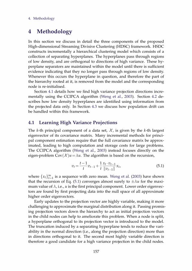
4. Methodology
4 Methodology
In this section we discuss in detail the three components of the proposedHigh-dimensional Streaming Divisive Clustering (HDSC) framework. HSDCconstructs incrementally a hierarchical clustering model which consists of acollection of separating hyperplanes. The hyperplanes pass through regionsof low density, and are orthogonal to directions of high variance. These hy-perplane separators are maintained within the model until there is sufficientevidence indicating that they no longer pass through regions of low density.Whenever this occurs the hyperplane in question, and therefore the part ofthe hierarchy rooted at it, is removed from the model and the correspondingnode is re-initialised.
Section 4.1 details how we find high variance projection directions incre-mentally using the CCIPCA algorithm (Weng et al., 2003). Section 4.2 de-scribes how low density hyperplanes are identified using information fromthe projected data only. In Section 4.3 we discuss how population drift canbe handled within this framework.
4.1 Learning High Variance Projections
The k-th principal component of a data set, X , is given by the k-th largesteigenvector of its covariance matrix. Many incremental methods for princi-pal component estimation require that the full covariance matrix be approx-imated, leading to high computation and storage costs for large problems.The CCIPCA algorithm (Weng et al., 2003) instead focuses directly on theeigen-problem Cov(X )u=λu. The algorithm is based on the recursion,
vt =t−1
tvt−1+
1t
xt ·vt−1
‖vt−1‖xt, (5.1)
where xt∞t=1 is a sequence with zero mean. Weng et al. (2003) have shown
that the recursion of Eq. (5.1) converges almost surely to ±λu for the maxi-mum value of λ, i.e., u is the first principal component. Lower order eigenvec-tors are found by first projecting data into the null space of all approximatehigher order eigenvectors.
Early updates to the projection vector are highly variable, making it morechallenging to approximate the marginal distribution along it. Passing promis-ing projection vectors down the hierarchy to act as initial projection vectorsin the child nodes can help to ameliorate this problem. When a node is split,a hyperplane orthogonal to its projection vector is introduced to the model.The truncation induced by a separating hyperplane tends to reduce the vari-ability in the normal direction (i.e., along the projection direction) more thanin directions orthogonal to it. The second most highly variable direction istherefore a good candidate for a high variance projection in the child nodes.
157
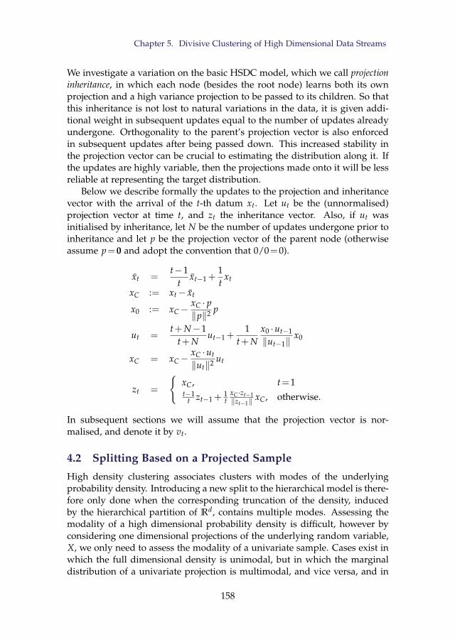
Chapter 5. Divisive Clustering of High Dimensional Data Streams
We investigate a variation on the basic HSDC model, which we call projectioninheritance, in which each node (besides the root node) learns both its ownprojection and a high variance projection to be passed to its children. So thatthis inheritance is not lost to natural variations in the data, it is given addi-tional weight in subsequent updates equal to the number of updates alreadyundergone. Orthogonality to the parent’s projection vector is also enforcedin subsequent updates after being passed down. This increased stability inthe projection vector can be crucial to estimating the distribution along it. Ifthe updates are highly variable, then the projections made onto it will be lessreliable at representing the target distribution.
Below we describe formally the updates to the projection and inheritancevector with the arrival of the t-th datum xt. Let ut be the (unnormalised)projection vector at time t, and zt the inheritance vector. Also, if ut wasinitialised by inheritance, let N be the number of updates undergone prior toinheritance and let p be the projection vector of the parent node (otherwiseassume p=0 and adopt the convention that 0/0=0).
xt =t−1
txt−1+
1t
xt
xC := xt− xt
x0 := xC−xC · p‖p‖2 p
ut =t+N−1
t+Nut−1+
1t+N
x0 ·ut−1
‖ut−1‖x0
xC = xC−xC ·ut
‖ut‖2 ut
zt =
xC, t=1t−1
t zt−1+1t
xC ·zt−1‖zt−1‖
xC, otherwise.
In subsequent sections we will assume that the projection vector is nor-malised, and denote it by vt.
4.2 Splitting Based on a Projected Sample
High density clustering associates clusters with modes of the underlyingprobability density. Introducing a new split to the hierarchical model is there-fore only done when the corresponding truncation of the density, inducedby the hierarchical partition of Rd, contains multiple modes. Assessing themodality of a high dimensional probability density is difficult, however byconsidering one dimensional projections of the underlying random variable,X, we only need to assess the modality of a univariate sample. Cases exist inwhich the full dimensional density is unimodal, but in which the marginaldistribution of a univariate projection is multimodal, and vice versa, and in
158
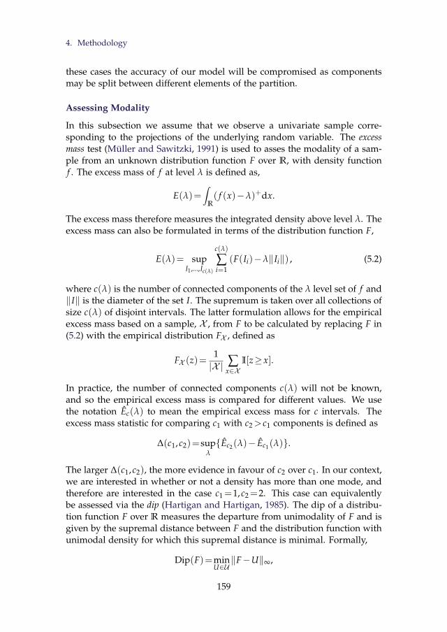
4. Methodology
these cases the accuracy of our model will be compromised as componentsmay be split between different elements of the partition.
Assessing Modality
In this subsection we assume that we observe a univariate sample corre-sponding to the projections of the underlying random variable. The excessmass test (Müller and Sawitzki, 1991) is used to asses the modality of a sam-ple from an unknown distribution function F over R, with density functionf . The excess mass of f at level λ is defined as,
E(λ)=∫
R( f (x)−λ)+dx.
The excess mass therefore measures the integrated density above level λ. Theexcess mass can also be formulated in terms of the distribution function F,
E(λ)= supI1,...,Ic(λ)
c(λ)
∑i=1
(F(Ii)−λ‖Ii‖) , (5.2)
where c(λ) is the number of connected components of the λ level set of f and‖I‖ is the diameter of the set I. The supremum is taken over all collections ofsize c(λ) of disjoint intervals. The latter formulation allows for the empiricalexcess mass based on a sample, X , from F to be calculated by replacing F in(5.2) with the empirical distribution FX , defined as
FX (z)=1|X | ∑
x∈XI[z≥ x].
In practice, the number of connected components c(λ) will not be known,and so the empirical excess mass is compared for different values. We usethe notation Ec(λ) to mean the empirical excess mass for c intervals. Theexcess mass statistic for comparing c1 with c2> c1 components is defined as
∆(c1, c2)=supλ
Ec2(λ)− Ec1(λ).
The larger ∆(c1, c2), the more evidence in favour of c2 over c1. In our context,we are interested in whether or not a density has more than one mode, andtherefore are interested in the case c1=1, c2=2. This case can equivalentlybe assessed via the dip (Hartigan and Hartigan, 1985). The dip of a distribu-tion function F over R measures the departure from unimodality of F and isgiven by the supremal distance between F and the distribution function withunimodal density for which this supremal distance is minimal. Formally,
Dip(F)=minU∈U‖F−U‖∞,
159
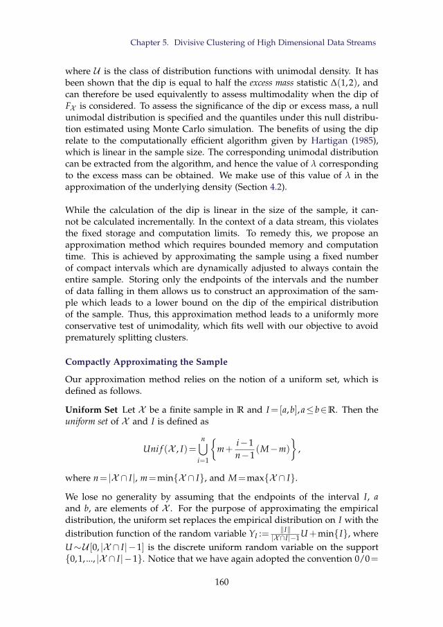
Chapter 5. Divisive Clustering of High Dimensional Data Streams
where U is the class of distribution functions with unimodal density. It hasbeen shown that the dip is equal to half the excess mass statistic ∆(1,2), andcan therefore be used equivalently to assess multimodality when the dip ofFX is considered. To assess the significance of the dip or excess mass, a nullunimodal distribution is specified and the quantiles under this null distribu-tion estimated using Monte Carlo simulation. The benefits of using the diprelate to the computationally efficient algorithm given by Hartigan (1985),which is linear in the sample size. The corresponding unimodal distributioncan be extracted from the algorithm, and hence the value of λ correspondingto the excess mass can be obtained. We make use of this value of λ in theapproximation of the underlying density (Section 4.2).
While the calculation of the dip is linear in the size of the sample, it can-not be calculated incrementally. In the context of a data stream, this violatesthe fixed storage and computation limits. To remedy this, we propose anapproximation method which requires bounded memory and computationtime. This is achieved by approximating the sample using a fixed numberof compact intervals which are dynamically adjusted to always contain theentire sample. Storing only the endpoints of the intervals and the numberof data falling in them allows us to construct an approximation of the sam-ple which leads to a lower bound on the dip of the empirical distributionof the sample. Thus, this approximation method leads to a uniformly moreconservative test of unimodality, which fits well with our objective to avoidprematurely splitting clusters.
Compactly Approximating the Sample
Our approximation method relies on the notion of a uniform set, which isdefined as follows.
Uniform Set Let X be a finite sample in R and I=[a,b], a≤b∈R. Then theuniform set of X and I is defined as
Uni f (X , I)=n⋃
i=1
m+
i−1n−1
(M−m)
,
where n= |X ∩ I|, m=minX ∩ I, and M=maxX ∩ I.
We lose no generality by assuming that the endpoints of the interval I, aand b, are elements of X . For the purpose of approximating the empiricaldistribution, the uniform set replaces the empirical distribution on I with thedistribution function of the random variable YI := ‖I‖
|X∩I|−1 U+minI, whereU∼U [0, |X ∩ I|−1] is the discrete uniform random variable on the support0,1, ..., |X ∩ I|−1. Notice that we have again adopted the convention 0/0=
160
4. Methodology
0. For a collection of disjoint intervals I1< I2< ...< Ik, which jointly containthe entire sample, the approximate distribution is given by,
F(x)=1|X |
k
∑i=1|X ∩ Ii|FYIi
,
where FYIiis the distribution function of YIi , defined as above.
With the arrival of a new datum, x, F must be updated such that the num-ber of intervals used does not exceed the predefined limit. If x lies withinone of the existing intervals, then no adjustment to the above formulation isnecessary. Otherwise, an interval I=[x, x] is added, and then two adjacent in-tervals are replaced with the convex hull of their union. The intervals mergedin this way are the adjacent pair which minimise the supremal distance be-tween F before and after the merger. If intervals i, i+1 are merged, then thisdistance is given by,
1|X |max
∣∣∣∣|X ∩ Ii|−⌈‖Ii‖‖Ii:i+1‖
⌉∣∣X ∩ Ii:i+1∣∣∣∣∣∣ ,∣∣∣∣|X ∩ Ii|+1−
⌈min Ii+1−min Ii‖Ii:i+1‖
⌉∣∣X ∩ Ii:i+1∣∣∣∣∣∣ ,
where Ii:i+1= Ii∪ Ii+1. With the above formulation of F we arrive at the fol-lowing result, the derivation of which can be found in the appendix. We alsodiscuss therein how a slight modification to the dip algorithm allows one tocalculate the dip of the sample approximation in O(k) time, where k is thenumber of intervals.
Lemma 28 Let X be a univariate sample of distinct points. For any collection ofdisjoint, compact intervals I1< I2< ...< Ik satisfying
X ⊂k⋃
j=1
Ij,
we have Dip(F)≤Dip(FX ).
This result ensures that the approximation method used cannot lead toadditional false discovery of multimodality when compared with the truesample of observations. While the result is stated for an unweighted sample,it also holds for weighted samples for which the data within each intervalare given the same weight. This is important as in the next subsection wedescribe how reweighting the data can be useful in better approximating thedistribution of a sample projected onto a vector which is continually beingupdated.
161
Chapter 5. Divisive Clustering of High Dimensional Data Streams
Accommodating a Shifting Projection
Our aim is to approximate the distribution of the projected random variable,v ·X, where ‖v‖=1. However, we only observe realisations of a sequence ofrandom variables vt ·Xt, where under the assumption that X1, X2, ... are i.i.d.,we know that vt converges almost surely to a vector v. Even under this as-sumption, the realisations vt · xt still represent a sample from a nonstationarydistribution due to the shifting projection vt. With consecutive updates to vt,the accuracy of the observed projections as a representation of the target dis-tribution diminishes. The influence of these observations on the approximatedistribution should therefore diminish with subsequent updates. Forgettingfactors impose a decaying weight mechanism to control the influence of pastobservations on the current estimate, however they are difficult to tune inpractice. If wt,i is the weight associated with observation i at time t, thenwt,i =(1−λt)wt−1,i, where λt∈ [0,1] is the forgetting factor at time t. Weightsassociated with new observations are initialised at 1, and so we have,
Wt :=t
∑i=1
wt,i = 1+(1−λt)t
∑i=1
wt−1,i
= 1+(1−λt)Wt−1.
Our approximate distribution F is a mixture of discrete uniform distribu-tions, in which the weight associated with each component is equal to thenumber of atoms in its support. Using forgetting factors we can adjust theseweights to obtain a more accurate approximation to the distribution on thecurrent projection. The update to F, which we now index by t to representthe approximation after t observations, is therefore given by,
Ft =1
WtFY[xt ,xt ]
+(1−λt)Wt−1
WtFt−1,
where xt is the observation at time t. If the number of intervals then exceedsthe upper limit, the merging of two adjacent intervals is performed as de-scribed in Section 4.2. As λt approaches zero, past and present observationsbecome equally weighted, while higher values of λt increase the influenceof recent observations on F. In problems with an explicit loss function, for-getting factors can be tuned using stochastic gradient descent (Haykin, 1999;Anagnostopoulos et al., 2012; Pavlidis et al., 2011), but this is not true in ourcontext. We propose an adaptive scheme which is complementary to the in-cremental estimation of the projection in that it uses information about theangles between consecutive updates to vt to quantify the variability of theprojected distribution over time. In detail, with the arrival of the (t+1)-thdatum, first vt is updated as described in Section 4.1, and then λt is set to,
λt+1=minΛ,γλt +(1−γ)arccos(vt+1 ·vt), (5.3)
162
4. Methodology
where Λ∈ (0,1] is a chosen maximum forgetting factor. We use an exponen-tially weighted moving average (EWMA) with parameter γ∈ (0,1) to smooththe impact on λt of isolated large fluctuations in arccos(vt+1 ·vt) arising fromnatural variation in vt. The following proposition states that the adaptivescheme of (5.3) converges almost surely to 0, whenever vt converges almostsurely. The distribution approximation will therefore stabilise as the projec-tion converges, which is almost sure under the CCIPCA algorithm as long asthe underlying distribution does not change.
Proposition 29 If vt∞t=1 converges almost surely and ‖vt‖=1 ∀t, then λt
a.s.−→0,where λt is as in (5.3).
Reweighting the projected data in this way means that the approximatedip or excess mass must be compared with the quantiles for a sample of sizeequal to the effective sample size of the reweighted data, which we calculate asthe sum of the weights in the approximation F.
When the null hypothesis of unimodality is rejected based on the dipof the approximate sample distribution, the associated node is split. Theprojection direction and split point are then kept fixed. In the following wedescribe how to approximate local minima in the density along the projection,thereby allowing one to determine such a split point based on this density.
Approximating Anti-modes
The distribution function F is discontinuous, and therefore using this dis-tribution directly to approximate an antimode in the underlying density ischallenging. A standard approach to generating smooth density approxima-tions is to consider a convolution with a smooth distribution function, havingdensity K. The density K is referred to as a kernel. The convolution of a dis-crete distribution associated with a random variable Y, having mass functionp(y), with a smooth distribution, gives rise to the canonical kernel densityestimate,
f (x)=1h ∑
y∈Support(Y)p(y)K
(x−y
h
).
The parameter h is called the bandwidth, and controls the smoothness of theresulting density estimate. A common choice of kernel is the standard Gaus-sian distribution given by,
K(x)=1√2π
e−x2/2.
In this case the bandwidth directly relates to the standard deviation of thesmoothing density. The support of the random variable underlying our ap-proximation F still contains |X | atoms, despite the compression of its rep-resentation. The evaluation of the associated kernel density estimate at a
163
Chapter 5. Divisive Clustering of High Dimensional Data Streams
fixed number of points is O(|X |). Knowledge that F represents a mixtureof discrete uniform distribution functions leads us to instead consider theconvolution of the corresponding continuous uniform distribution functionswith the kernel K. For those intervals which contain only a single point, thereis no associated continuous distribution, and so the standard kernel convolu-tion above is used. The convolution of the uniform density on [a,b], a<b∈R
with the Gaussian distribution with variance h2 is given by
f (x)=Φ((x− a)/h)−Φ((x−b)/h)
b− a,
where Φ is the distribution function of the standard Gaussian random vari-able. With this formulation the associated kernel density estimate has k com-ponents, rather than |X |.
How to choose h remains a very active area of research, and no universalguidelines exist for every context. We use the equivalence of the dip and ex-cess mass tests, and the implications of the rejection of their null hypotheses,to inform our choice of h. Rejection of the null hypothesis of the excess masstest is equivalent to favouring two λ level set components over one. The cor-responding value of λ can be extracted from the dip algorithm. We chooseh such that the associated density estimate has λ level set consisting of twocomponents. The minimum such value of h is chosen, as this leads to moresharply defined modes and anti-modes.
4.3 Handling Population Drift
A generic approach to detect time-variations in f that invalidate our clus-tering model is to sequentially consider the hypothesis that each hyperplanepasses through a region of low relative f density (low-density separation hy-pothesis). If this hypothesis is false then a revision of the corresponding partof the hierarchical model is necessary. Notice that the low-density separa-tion hypothesis is not a hypothesis of overall stationarity of f . Indeed, asFigure 5.1 shows, considerable variation in f is possible without invalidatingthe model. The figure also shows that testing this hypothesis for all separat-ing hyperplanes enables us to identify and revise only the relevant part ofthe clustering hierarchy when a change is detected, rather than resetting theentire model. Moreover, the low-density separation hypothesis is indepen-dent of the type (abrupt, or gradual) and the speed of drift. Lastly, testingthis hypothesis corresponds to a one-dimensional change detection problem,since each low-density hyperplane is identified through an estimate of a one-dimensional marginal density.
With each hyperplane added to the model we initialise a Bernoulli CUSUMchange detection regime, as described in Reynolds and Stoumbos (1999), to
164
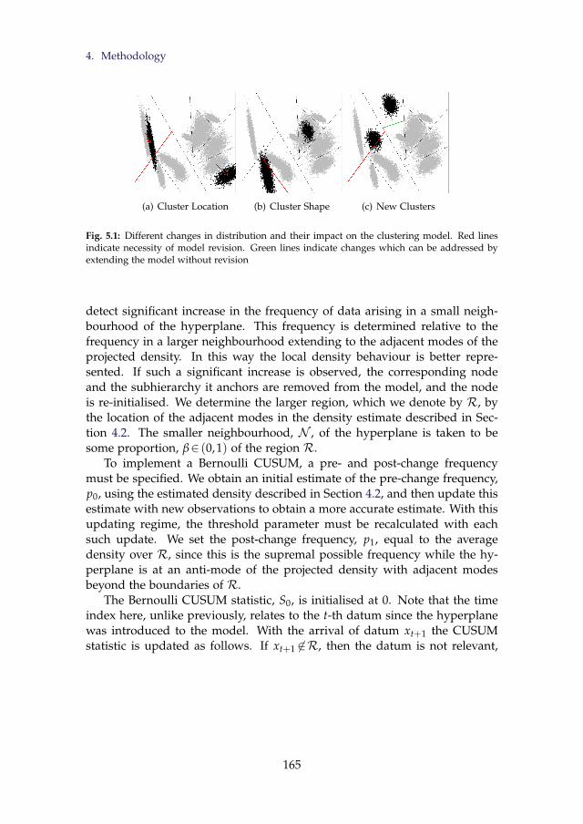
4. Methodology
(a) Cluster Location (b) Cluster Shape (c) New Clusters
Fig. 5.1: Different changes in distribution and their impact on the clustering model. Red linesindicate necessity of model revision. Green lines indicate changes which can be addressed byextending the model without revision
detect significant increase in the frequency of data arising in a small neigh-bourhood of the hyperplane. This frequency is determined relative to thefrequency in a larger neighbourhood extending to the adjacent modes of theprojected density. In this way the local density behaviour is better repre-sented. If such a significant increase is observed, the corresponding nodeand the subhierarchy it anchors are removed from the model, and the nodeis re-initialised. We determine the larger region, which we denote by R, bythe location of the adjacent modes in the density estimate described in Sec-tion 4.2. The smaller neighbourhood, N , of the hyperplane is taken to besome proportion, β∈ (0,1) of the region R.
To implement a Bernoulli CUSUM, a pre- and post-change frequencymust be specified. We obtain an initial estimate of the pre-change frequency,p0, using the estimated density described in Section 4.2, and then update thisestimate with new observations to obtain a more accurate estimate. With thisupdating regime, the threshold parameter must be recalculated with eachsuch update. We set the post-change frequency, p1, equal to the averagedensity over R, since this is the supremal possible frequency while the hy-perplane is at an anti-mode of the projected density with adjacent modesbeyond the boundaries of R.
The Bernoulli CUSUM statistic, S0, is initialised at 0. Note that the timeindex here, unlike previously, relates to the t-th datum since the hyperplanewas introduced to the model. With the arrival of datum xt+1 the CUSUMstatistic is updated as follows. If xt+1 6∈R, then the datum is not relevant,
165
Chapter 5. Divisive Clustering of High Dimensional Data Streams
and St+1=St. If xt+1∈R, then,
B =
1, if xt+1∈N0, otherwise
,
St+1 = max0,St+B
+ log(
1− p1
1− p0
)log(
p1(1− p0)
p0(1− p1)
)−1
.
A change is detected when St exceeds a threshold α. We set α conserva-tively, corresponding to the maximum for chosen run lengths under p0 andp1, which we calculate according to the method in Reynolds and Stoumbos(1999).
5 The HSDC Algorithm
Having detailed the constituent elements of the method in Section 4, in thissection we give a brief summary of the overall algorithm. The clusteringmodel constructed by HSDC comprises a hierarchy of separating hyper-planes, each defined by a projection vector, v∈Rd, of norm 1, and split pointb∈R. Associated with each hyperplane is a CUSUM statistic, S, in placeto detect changes in the underlying distribution which lead to instability ofthe clustering result. The leaf nodes of the hierarchy (i.e. those for whichthe truncated density has not been deemed multimodal) each have associ-ated with them an updating projection, as well as an approximate univariatedistribution associated with the projection onto it. Leaf nodes might alsocontain inheritance vectors, z, to be passed to their children as projections inthe event that the node is split.
Algorithm 3 describes an update to the hierarchical model with the arrivalof a datum x. We associate with each node an identifying tag, ID, which in-forms the algorithm where to direct data down the hierarchy. Each internalnode has 2 children, LChild and RChild, associated with the halfspaces in-duced by the node’s hyperplane.
The datum traverses the hierarchical structure until it reaches the appro-priate leaf node. At each internal node along its path, the correspondingCUSUM statistic is updated as in Section 4.3. If a change is detected, the as-sociated node is reinitialised, and it becomes a leaf. Otherwise, the datum isprojected onto the node’s projection vector, and is passed to the appropriatechild node. Once the datum arrives at a leaf, the leaf’s projection vector is up-dated as described in Section 4.1. The datum is projected onto this updatedvector, and this projected datum is used to update the node’s sample approx-imation, as described in Sections 4.2 and 4.2. The dip statistic of the sample
166
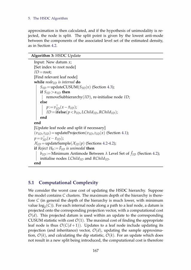
5. The HSDC Algorithm
approximation is then calculated, and if the hypothesis of unimodality is re-jected, the node is split. The split point is given by the lowest anti-modebetween the components of the associated level set of the estimated density,as in Section 4.2.
Algorithm 3: HSDC Update
Input: New datum x;[Set index to root node]ID= root;[Find relevant leaf node]while nodeID is internal do
SID =updateCUSUM(SID|x) (Section 4.3);if SID >αID then
removeSubhierarchy(ID), re-initialise node ID;else
p :=v>ID(x− xID);ID= ifelse(p<bID, LChildID, RChildID);
endend[Update leaf node and split if necessary](vID,zID)=updateProjection(vID,zID|x) (Section 4.1);p=v>ID(x− xID);XID =updateSample(XID|p) (Sections 4.2-4.2);if Reject H0 := FID is unimodal then
bID :=Minimum Antimode Between λ Level Set of f ID (Section 4.2);initialise nodes LChildID and RChildID.
end
5.1 Computational Complexity
We consider the worst case cost of updating the HSDC hierarchy. Supposethe model contains C clusters. The maximum depth of the hierarchy is there-fore C (in general the depth of the hierarchy is much lower, with minimumvalue log2(C)). For each internal node along a path to a leaf node, a datum isprojected onto the corresponding projection vector, with a computational costO(d). This projected datum is used within an update to the correspondingCUSUM statistic with cost O(1). The maximal cost of finding the appropriateleaf node is thus O(C(d+1)). Updates to a leaf node include updating itsprojection (and inheritance) vector, O(d), updating the sample approxima-tion, O(k), and calculating the dip statistic, O(k). For an update which doesnot result in a new split being introduced, the computational cost is therefore
167
Chapter 5. Divisive Clustering of High Dimensional Data Streams
O((C+1)(d+1)+ k). In high dimensional applications, we have Cd k, andso the behaviour is O((C+1)(d+1)).
When a node is split, we determine the minimum bandwidth, h, giv-ing the correct level set of the density estimate. This is done by a bisectionmethod, which has log2((hmax−hmin)/ε) iterations, where hmax and hmin areupper and lower bounds on h respectively, and ε is the tolerance level. Withineach iteration, the kernel density estimate is calculated, at a cost of O(k2).The split point is calculated within this procedure.
For existing data stream clustering algorithms based on microclusters,the primary cost associated with the online step lies in determining thenearest microcluster. This has computational cost O(md), where m is thenumber of microclusters. The time complexity of the offline step dependson the clustering algorithm being employed. Algorithms based on k-meansare technically NP hard, however practical implementations run in O(mkd)time. Density connectivity methods based on DBSCAN have time complexityO(dm log(m)).
Density based methods based on grids have time complexity of the onlinestep O(g), where g is the number of active grid cells. Without pruning meth-ods, this is exponential in d (Aggarwal, 2013). For the offline component, theapproach of DStream (Chen et al., 2007) only requires processing those gridcells which changed since the last offline step. If t is the number of time stepssince the last offline step, the computational cost is O(t). This means that thetotal cost of all offline steps up to time point T has worst case cost O(T).
In general the number of microcluster and grids cells is substantiallylarger than the actual number of clusters, i.e., Cm, g. (The HPStream al-gorithm is an exception.) For standard updates therefore HSDC comparesfavourably with existing data stream clustering algorithms in terms of updatetime, especially on high dimensional examples. Updates to HSDC which re-sult in the introduction of a new split have an additional cost of O(k2). How-ever, in practice these updates requiring a new split being introduced are in-frequent, and the overall complexity is dominated by standard update steps.Most importantly however, HSDC has no offline clustering component.
6 Experimental Results
We compare the performance of the following methods.
1. CluStream (Aggarwal et al., 2003): We use the implementation in the Rpackage streamMOA, and the parameters suggested in (Aggarwal et al.,2003).
2. HPStream (Aggarwal et al., 2004): HPStream, like CluStream, requiresan offline initialisation step, for which we give it 2000 data and provide
168
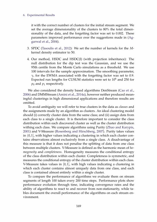
6. Experimental Results
it with the correct number of clusters for the initial stream segment. Weset the average dimensionality of the clusters to 80% the total dimen-sionality of the data, and the forgetting factor was set to 0.002. Theseparameters improved performance over the suggestions made in (Ag-garwal et al., 2004).
3. SPDC (Tasoulis et al., 2012): We set the number of kernels for the M-kernel density estimator to 50.
4. Our method, HSDC and HSDC(I) (with projection inheritance): Thenull distribution for the dip test was the Gaussian, and we use the95th centile from the Monte Carlo simulations as a threshold. We use100 intervals for the sample approximation. The smoothing parameter,γ, for the EWMA associated with the forgetting factor was set to 0.9.Expected run lengths for CUSUM statistics were set to 106 and 250 forp0 and p1 respectively.
We also considered the density based algorithms DenStream (Cao et al.,2006) and DMMStream (Amini et al., 2014a), however neither produced mean-ingful clusterings in high dimensional applications and therefore results areomitted.
To avoid ambiguity we will refer to true clusters in the data as classes andthe assignments made by an algorithm as clusters. An ideal clustering modelshould (i) correctly cluster data from the same class; and (ii) assign data fromeach class to a single cluster. It is therefore important to consider the classdistribution within each discovered cluster as well as the cluster distributionwithing each class. We compare algorithms using Purity (Zhao and Karypis,2001) and V-Measure (Rosenberg and Hirschberg, 2007). Purity takes valuesin (0,1], with higher values indicating a clustering in which each cluster con-tains observations almost exclusively from a single class. A disadvantage ofthis measure is that it does not penalise the splitting of data from one classbetween multiple clusters. V-Measure is defined as the harmonic mean of ho-mogeneity and completeness. Homogeneity measures the conditional entropyof the class distribution within each cluster. Completeness is symmetric, andmeasures the conditional entropy of the cluster distribution within each class.V-Measure takes values in [0,1], with high values indicating a clustering inwhich each cluster contains almost uniquely data from one class, and eachclass is contained almost entirely within a single cluster.
To compare the performance of algorithms we evaluate them on streamsegments of length 100 taken every 200 time steps. Performance plots showperformance evolution through time, indicating convergence rates and theability of algorithms to react to and recover from non-stationarity, while ta-bles document the overall performance of the algorithms on each stream en-vironment.
169
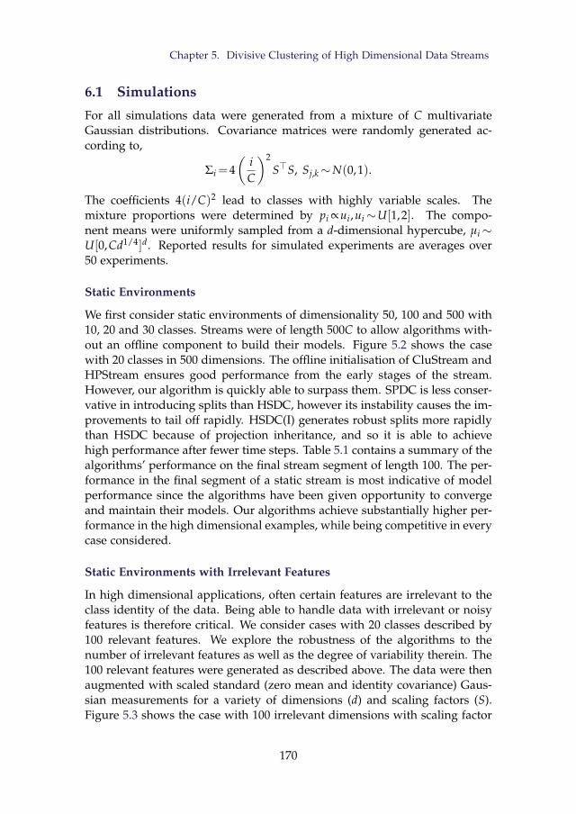
Chapter 5. Divisive Clustering of High Dimensional Data Streams
6.1 Simulations
For all simulations data were generated from a mixture of C multivariateGaussian distributions. Covariance matrices were randomly generated ac-cording to,
Σi =4(
iC
)2S>S, Sj,k∼N(0,1).
The coefficients 4(i/C)2 lead to classes with highly variable scales. Themixture proportions were determined by pi ∝ ui,ui∼U[1,2]. The compo-nent means were uniformly sampled from a d-dimensional hypercube, µi∼U[0,Cd1/4]d. Reported results for simulated experiments are averages over50 experiments.
Static Environments
We first consider static environments of dimensionality 50, 100 and 500 with10, 20 and 30 classes. Streams were of length 500C to allow algorithms with-out an offline component to build their models. Figure 5.2 shows the casewith 20 classes in 500 dimensions. The offline initialisation of CluStream andHPStream ensures good performance from the early stages of the stream.However, our algorithm is quickly able to surpass them. SPDC is less conser-vative in introducing splits than HSDC, however its instability causes the im-provements to tail off rapidly. HSDC(I) generates robust splits more rapidlythan HSDC because of projection inheritance, and so it is able to achievehigh performance after fewer time steps. Table 5.1 contains a summary of thealgorithms’ performance on the final stream segment of length 100. The per-formance in the final segment of a static stream is most indicative of modelperformance since the algorithms have been given opportunity to convergeand maintain their models. Our algorithms achieve substantially higher per-formance in the high dimensional examples, while being competitive in everycase considered.
Static Environments with Irrelevant Features
In high dimensional applications, often certain features are irrelevant to theclass identity of the data. Being able to handle data with irrelevant or noisyfeatures is therefore critical. We consider cases with 20 classes described by100 relevant features. We explore the robustness of the algorithms to thenumber of irrelevant features as well as the degree of variability therein. The100 relevant features were generated as described above. The data were thenaugmented with scaled standard (zero mean and identity covariance) Gaus-sian measurements for a variety of dimensions (d) and scaling factors (S).Figure 5.3 shows the case with 100 irrelevant dimensions with scaling factor
170
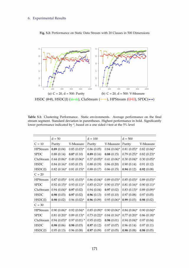
6. Experimental Results
Fig. 5.2: Performance on Static Data Stream with 20 Classes in 500 Dimensions
0 2000 4000 6000 8000 10000
0.5
0.6
0.7
0.8
0.9
1.0
(a) C = 20, d = 500: Purity
0 2000 4000 6000 8000 10000
0.5
0.6
0.7
0.8
0.9
1.0
(b) C = 20, d = 500: V-Measure
HSDC (0 0), HSDC(I) (4 4), CluStream (+ +), HPStream ( ), SPDC(∗ ∗)
Table 5.1: Clustering Performance. Static environments. Average performance on the finalstream segment. Standard deviation in parentheses. Highest performance in bold. Significantlylower performance indicated by *, based on a one sided t-test at the 5% level
d = 50 d = 100 d = 500
C = 10 Purity V-Measure Purity V-Measure Purity V-Measure
HPStream 0.89 (0.04) 0.85 (0.03)* 0.86 (0.05) 0.84 (0.04)* 0.81 (0.05)* 0.82 (0.04)*
SPDC 0.88 (0.14) 0.87 (0.10) 0.89 (0.16) 0.88 (0.15) 0.79 (0.25)* 0.82 (0.23)*
CluStream 0.44 (0.06)* 0.49 (0.06)* 0.37 (0.05)* 0.41 (0.06)* 0.30 (0.04)* 0.30 (0.05)*
HSDC 0.84 (0.16)* 0.83 (0.15) 0.88 (0.19) 0.86 (0.20) 0.90 (0.14) 0.91 (0.12)
HSDC(I) 0.82 (0.16)* 0.81 (0.15)* 0.88 (0.17) 0.86 (0.15) 0.94 (0.12) 0.92 (0.08)
C = 20
HPStream 0.87 (0.05)* 0.91 (0.03)* 0.86 (0.04)* 0.89 (0.03)* 0.85 (0.03)* 0.89 (0.03)*
SPDC 0.92 (0.15)* 0.93 (0.11)* 0.85 (0.21)* 0.90 (0.15)* 0.81 (0.16)* 0.90 (0.11)*
CluStream 0.94 (0.04)* 0.97 (0.02) 0.94 (0.04) 0.97 (0.02) 0.83 (0.13)* 0.89 (0.09)*
HSDC 0.98 (0.03) 0.97 (0.02) 0.96 (0.13) 0.95 (0.10) 0.97 (0.08) 0.97 (0.05)
HSDC(I) 0.98 (0.02) 0.96 (0.02)* 0.96 (0.09) 0.95 (0.06)* 0.99 (0.03) 0.98 (0.02)
C = 30
HPStream 0.90 (0.06)* 0.92 (0.04)* 0.85 (0.09)* 0.90 (0.06)* 0.84 (0.06)* 0.90 (0.04)*
SPDC 0.81 (0.20)* 0.89 (0.13)* 0.73 (0.22)* 0.84 (0.16)* 0.77 (0.20)* 0.86 (0.18)*
CluStream 0.94 (0.03)* 0.97 (0.01) * 0.95 (0.02) 0.98 (0.01) 0.94 (0.04)* 0.97 (0.04)
HSDC 0.98 (0.06) 0.98 (0.03) 0.97 (0.12) 0.97 (0.07) 0.96 (0.14) 0.97 (0.11)
HSDC(I) 0.95 (0.13) 0.96 (0.08) 0.97 (0.09) 0.97 (0.05) 0.98 (0.08) 0.98 (0.05)
171
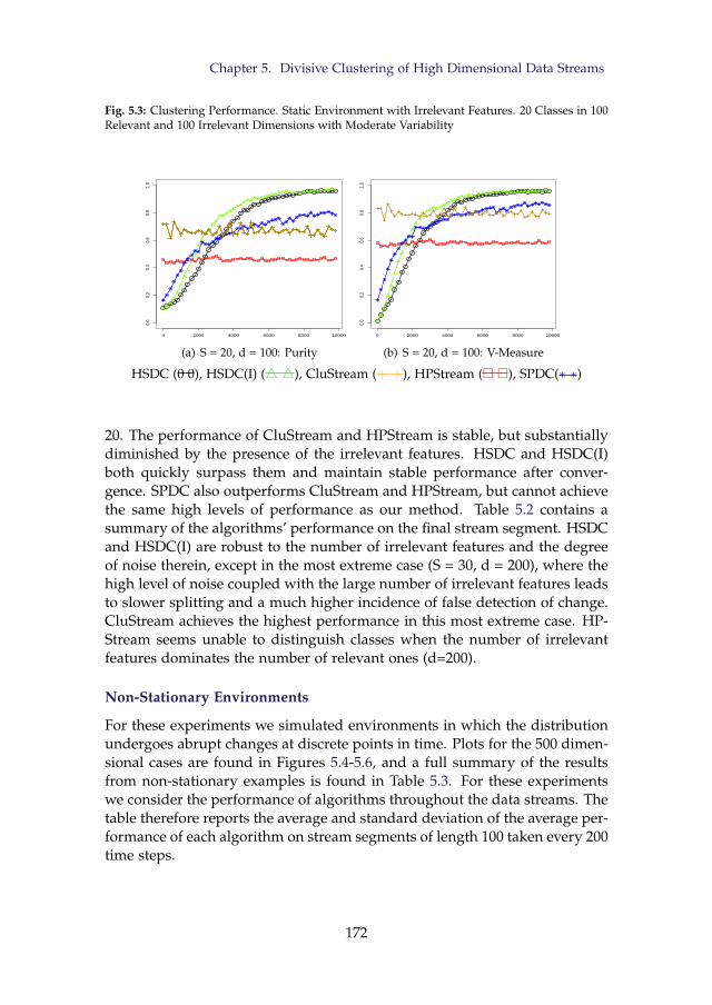
Chapter 5. Divisive Clustering of High Dimensional Data Streams
Fig. 5.3: Clustering Performance. Static Environment with Irrelevant Features. 20 Classes in 100Relevant and 100 Irrelevant Dimensions with Moderate Variability
0 2000 4000 6000 8000 10000
0.0
0.2
0.4
0.6
0.8
1.0
(a) S = 20, d = 100: Purity
0 2000 4000 6000 8000 10000
0.0
0.2
0.4
0.6
0.8
1.0
(b) S = 20, d = 100: V-Measure
HSDC (0 0), HSDC(I) (4 4), CluStream (+ +), HPStream ( ), SPDC(∗ ∗)
20. The performance of CluStream and HPStream is stable, but substantiallydiminished by the presence of the irrelevant features. HSDC and HSDC(I)both quickly surpass them and maintain stable performance after conver-gence. SPDC also outperforms CluStream and HPStream, but cannot achievethe same high levels of performance as our method. Table 5.2 contains asummary of the algorithms’ performance on the final stream segment. HSDCand HSDC(I) are robust to the number of irrelevant features and the degreeof noise therein, except in the most extreme case (S = 30, d = 200), where thehigh level of noise coupled with the large number of irrelevant features leadsto slower splitting and a much higher incidence of false detection of change.CluStream achieves the highest performance in this most extreme case. HP-Stream seems unable to distinguish classes when the number of irrelevantfeatures dominates the number of relevant ones (d=200).
Non-Stationary Environments
For these experiments we simulated environments in which the distributionundergoes abrupt changes at discrete points in time. Plots for the 500 dimen-sional cases are found in Figures 5.4-5.6, and a full summary of the resultsfrom non-stationary examples is found in Table 5.3. For these experimentswe consider the performance of algorithms throughout the data streams. Thetable therefore reports the average and standard deviation of the average per-formance of each algorithm on stream segments of length 100 taken every 200time steps.
172
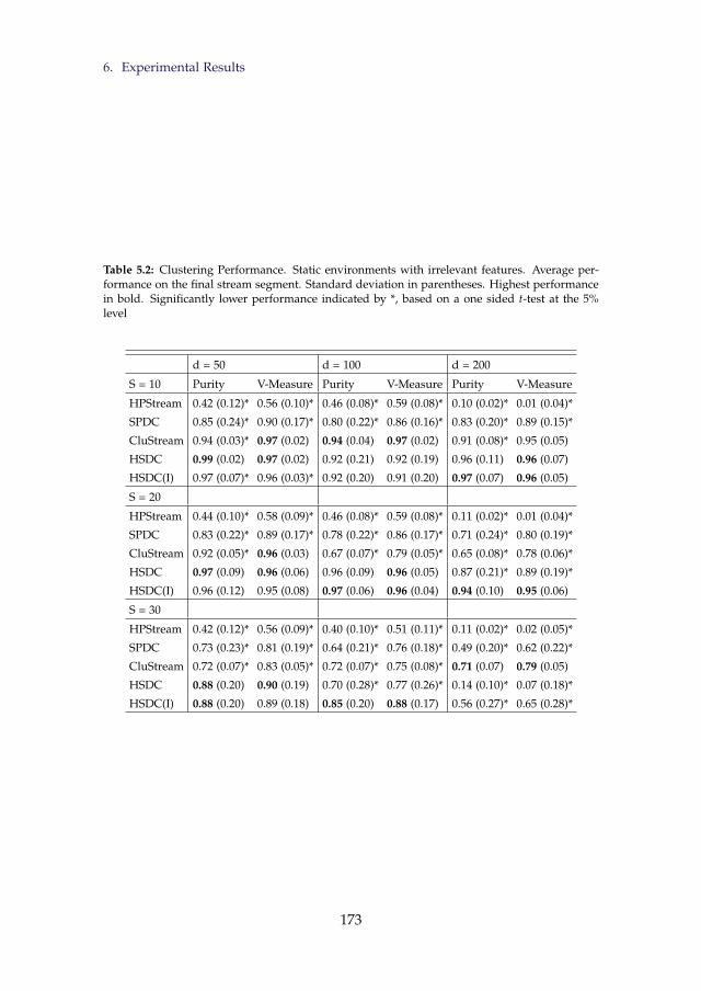
6. Experimental Results
Table 5.2: Clustering Performance. Static environments with irrelevant features. Average per-formance on the final stream segment. Standard deviation in parentheses. Highest performancein bold. Significantly lower performance indicated by *, based on a one sided t-test at the 5%level
d = 50 d = 100 d = 200
S = 10 Purity V-Measure Purity V-Measure Purity V-Measure
HPStream 0.42 (0.12)* 0.56 (0.10)* 0.46 (0.08)* 0.59 (0.08)* 0.10 (0.02)* 0.01 (0.04)*
SPDC 0.85 (0.24)* 0.90 (0.17)* 0.80 (0.22)* 0.86 (0.16)* 0.83 (0.20)* 0.89 (0.15)*
CluStream 0.94 (0.03)* 0.97 (0.02) 0.94 (0.04) 0.97 (0.02) 0.91 (0.08)* 0.95 (0.05)
HSDC 0.99 (0.02) 0.97 (0.02) 0.92 (0.21) 0.92 (0.19) 0.96 (0.11) 0.96 (0.07)
HSDC(I) 0.97 (0.07)* 0.96 (0.03)* 0.92 (0.20) 0.91 (0.20) 0.97 (0.07) 0.96 (0.05)
S = 20
HPStream 0.44 (0.10)* 0.58 (0.09)* 0.46 (0.08)* 0.59 (0.08)* 0.11 (0.02)* 0.01 (0.04)*
SPDC 0.83 (0.22)* 0.89 (0.17)* 0.78 (0.22)* 0.86 (0.17)* 0.71 (0.24)* 0.80 (0.19)*
CluStream 0.92 (0.05)* 0.96 (0.03) 0.67 (0.07)* 0.79 (0.05)* 0.65 (0.08)* 0.78 (0.06)*
HSDC 0.97 (0.09) 0.96 (0.06) 0.96 (0.09) 0.96 (0.05) 0.87 (0.21)* 0.89 (0.19)*
HSDC(I) 0.96 (0.12) 0.95 (0.08) 0.97 (0.06) 0.96 (0.04) 0.94 (0.10) 0.95 (0.06)
S = 30
HPStream 0.42 (0.12)* 0.56 (0.09)* 0.40 (0.10)* 0.51 (0.11)* 0.11 (0.02)* 0.02 (0.05)*
SPDC 0.73 (0.23)* 0.81 (0.19)* 0.64 (0.21)* 0.76 (0.18)* 0.49 (0.20)* 0.62 (0.22)*
CluStream 0.72 (0.07)* 0.83 (0.05)* 0.72 (0.07)* 0.75 (0.08)* 0.71 (0.07) 0.79 (0.05)
HSDC 0.88 (0.20) 0.90 (0.19) 0.70 (0.28)* 0.77 (0.26)* 0.14 (0.10)* 0.07 (0.18)*
HSDC(I) 0.88 (0.20) 0.89 (0.18) 0.85 (0.20) 0.88 (0.17) 0.56 (0.27)* 0.65 (0.28)*
173
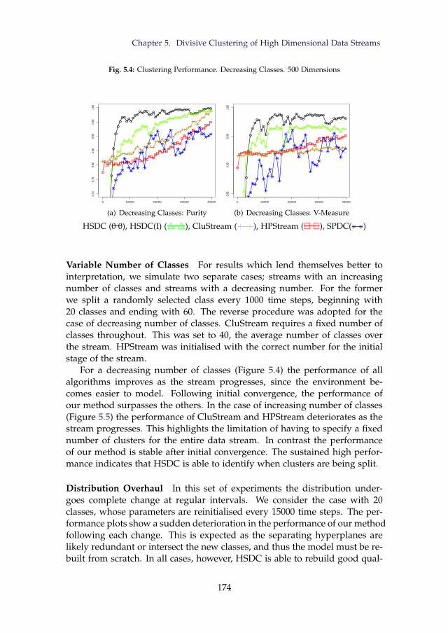
Chapter 5. Divisive Clustering of High Dimensional Data Streams
Fig. 5.4: Clustering Performance. Decreasing Classes. 500 Dimensions
0 10000 20000 30000 40000
0.70
0.75
0.80
0.85
0.90
0.95
1.00
(a) Decreasing Classes: Purity
0 10000 20000 30000 40000
0.85
0.90
0.95
1.00
(b) Decreasing Classes: V-Measure
HSDC (0 0), HSDC(I) (4 4), CluStream (+ +), HPStream ( ), SPDC(∗ ∗)
Variable Number of Classes For results which lend themselves better tointerpretation, we simulate two separate cases; streams with an increasingnumber of classes and streams with a decreasing number. For the formerwe split a randomly selected class every 1000 time steps, beginning with20 classes and ending with 60. The reverse procedure was adopted for thecase of decreasing number of classes. CluStream requires a fixed number ofclasses throughout. This was set to 40, the average number of classes overthe stream. HPStream was initialised with the correct number for the initialstage of the stream.
For a decreasing number of classes (Figure 5.4) the performance of allalgorithms improves as the stream progresses, since the environment be-comes easier to model. Following initial convergence, the performance ofour method surpasses the others. In the case of increasing number of classes(Figure 5.5) the performance of CluStream and HPStream deteriorates as thestream progresses. This highlights the limitation of having to specify a fixednumber of clusters for the entire data stream. In contrast the performanceof our method is stable after initial convergence. The sustained high perfor-mance indicates that HSDC is able to identify when clusters are being split.
Distribution Overhaul In this set of experiments the distribution under-goes complete change at regular intervals. We consider the case with 20classes, whose parameters are reinitialised every 15000 time steps. The per-formance plots show a sudden deterioration in the performance of our methodfollowing each change. This is expected as the separating hyperplanes arelikely redundant or intersect the new classes, and thus the model must be re-built from scratch. In all cases, however, HSDC is able to rebuild good qual-
174
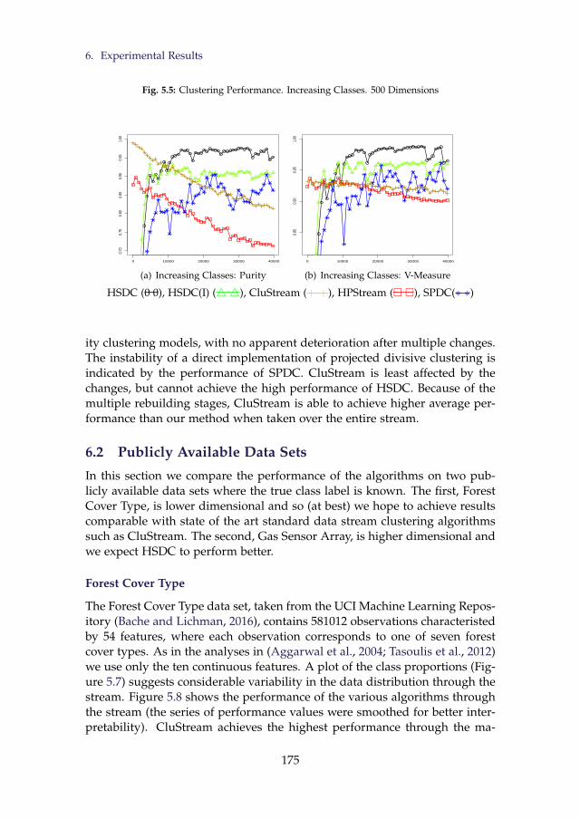
6. Experimental Results
Fig. 5.5: Clustering Performance. Increasing Classes. 500 Dimensions
0 10000 20000 30000 40000
0.70
0.75
0.80
0.85
0.90
0.95
1.00
(a) Increasing Classes: Purity
0 10000 20000 30000 40000
0.85
0.90
0.95
1.00
(b) Increasing Classes: V-Measure
HSDC (0 0), HSDC(I) (4 4), CluStream (+ +), HPStream ( ), SPDC(∗ ∗)
ity clustering models, with no apparent deterioration after multiple changes.The instability of a direct implementation of projected divisive clustering isindicated by the performance of SPDC. CluStream is least affected by thechanges, but cannot achieve the high performance of HSDC. Because of themultiple rebuilding stages, CluStream is able to achieve higher average per-formance than our method when taken over the entire stream.
6.2 Publicly Available Data Sets
In this section we compare the performance of the algorithms on two pub-licly available data sets where the true class label is known. The first, ForestCover Type, is lower dimensional and so (at best) we hope to achieve resultscomparable with state of the art standard data stream clustering algorithmssuch as CluStream. The second, Gas Sensor Array, is higher dimensional andwe expect HSDC to perform better.
Forest Cover Type
The Forest Cover Type data set, taken from the UCI Machine Learning Repos-itory (Bache and Lichman, 2016), contains 581012 observations characteristedby 54 features, where each observation corresponds to one of seven forestcover types. As in the analyses in (Aggarwal et al., 2004; Tasoulis et al., 2012)we use only the ten continuous features. A plot of the class proportions (Fig-ure 5.7) suggests considerable variability in the data distribution through thestream. Figure 5.8 shows the performance of the various algorithms throughthe stream (the series of performance values were smoothed for better inter-pretability). CluStream achieves the highest performance through the ma-
175
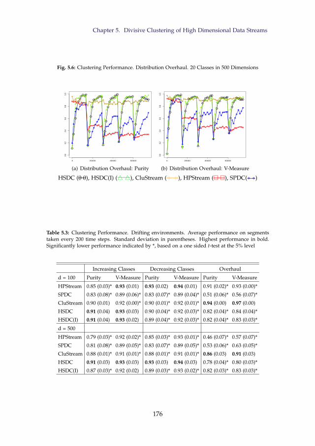
Chapter 5. Divisive Clustering of High Dimensional Data Streams
Fig. 5.6: Clustering Performance. Distribution Overhaul. 20 Classes in 500 Dimensions
0 20000 40000 60000
0.0
0.2
0.4
0.6
0.8
1.0
(a) Distribution Overhaul: Purity
0 20000 40000 600000.
00.
20.
40.
60.
81.
0
(b) Distribution Overhaul: V-Measure
HSDC (0 0), HSDC(I) (4 4), CluStream (+ +), HPStream ( ), SPDC(∗ ∗)
Table 5.3: Clustering Performance. Drifting environments. Average performance on segmentstaken every 200 time steps. Standard deviation in parentheses. Highest performance in bold.Significantly lower performance indicated by *, based on a one sided t-test at the 5% level
Increasing Classes Decreasing Classes Overhaul
d = 100 Purity V-Measure Purity V-Measure Purity V-Measure
HPStream 0.85 (0.03)* 0.93 (0.01) 0.93 (0.02) 0.94 (0.01) 0.91 (0.02)* 0.93 (0.00)*
SPDC 0.83 (0.08)* 0.89 (0.06)* 0.83 (0.07)* 0.89 (0.04)* 0.51 (0.06)* 0.56 (0.07)*
CluStream 0.90 (0.01) 0.92 (0.00)* 0.90 (0.01)* 0.92 (0.01)* 0.94 (0.00) 0.97 (0.00)
HSDC 0.91 (0.04) 0.93 (0.03) 0.90 (0.04)* 0.92 (0.03)* 0.82 (0.04)* 0.84 (0.04)*
HSDC(I) 0.91 (0.04) 0.93 (0.02) 0.89 (0.04)* 0.92 (0.03)* 0.82 (0.04)* 0.83 (0.03)*
d = 500
HPStream 0.79 (0.03)* 0.92 (0.02)* 0.85 (0.03)* 0.93 (0.01)* 0.46 (0.07)* 0.57 (0.07)*
SPDC 0.81 (0.08)* 0.89 (0.05)* 0.83 (0.07)* 0.89 (0.05)* 0.53 (0.06)* 0.63 (0.05)*
CluStream 0.88 (0.01)* 0.91 (0.01)* 0.88 (0.01)* 0.91 (0.01)* 0.86 (0.03) 0.91 (0.03)
HSDC 0.91 (0.03) 0.93 (0.03) 0.93 (0.03) 0.94 (0.03) 0.78 (0.04)* 0.80 (0.03)*
HSDC(I) 0.87 (0.03)* 0.92 (0.02) 0.89 (0.03)* 0.93 (0.02)* 0.82 (0.03)* 0.83 (0.03)*
176
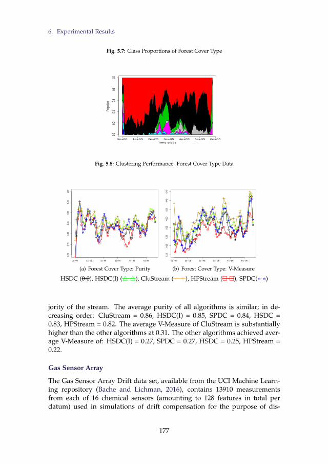
6. Experimental Results
Fig. 5.7: Class Proportions of Forest Cover Type
0e+00 1e+05 2e+05 3e+05 4e+05 5e+05 6e+05
0.00.2
0.40.6
0.81.0
Time steps
Prop
ortion
Fig. 5.8: Clustering Performance. Forest Cover Type Data
0e+00 1e+05 2e+05 3e+05 4e+05 5e+05
0.70
0.75
0.80
0.85
0.90
0.95
1.00
(a) Forest Cover Type: Purity
0e+00 1e+05 2e+05 3e+05 4e+05 5e+05
0.10
0.15
0.20
0.25
0.30
0.35
0.40
0.45
(b) Forest Cover Type: V-Measure
HSDC (0 0), HSDC(I) (4 4), CluStream (+ +), HPStream ( ), SPDC(∗ ∗)
jority of the stream. The average purity of all algorithms is similar; in de-creasing order: CluStream = 0.86, HSDC(I) = 0.85, SPDC = 0.84, HSDC =0.83, HPStream = 0.82. The average V-Measure of CluStream is substantiallyhigher than the other algorithms at 0.31. The other algorithms achieved aver-age V-Measure of: HSDC(I) = 0.27, SPDC = 0.27, HSDC = 0.25, HPStream =0.22.
Gas Sensor Array
The Gas Sensor Array Drift data set, available from the UCI Machine Learn-ing repository (Bache and Lichman, 2016), contains 13910 measurementsfrom each of 16 chemical sensors (amounting to 128 features in total perdatum) used in simulations of drift compensation for the purpose of dis-
177
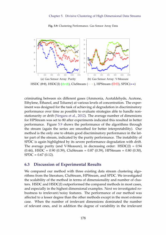
Chapter 5. Divisive Clustering of High Dimensional Data Streams
Fig. 5.9: Clustering Performance. Gas Sensor Array Data
0 2000 4000 6000 8000 10000 12000
0.5
0.6
0.7
0.8
0.9
1.0
(a) Gas Sensor Array: Purity
0 2000 4000 6000 8000 10000 12000
0.0
0.1
0.2
0.3
0.4
0.5
0.6
0.7
(b) Gas Sensor Array: V-Measure
HSDC (0 0), HSDC(I) (4 4), CluStream (+ +), HPStream ( ), SPDC(∗ ∗)
criminating between six different gases (Ammonia, Acetaldehyde, Acetone,Ethylene, Ethanol, and Toluene) at various levels of concentration. The exper-iment was designed for the task of achieving al degradation in discriminatoryperformance over time as possible to evaluate strategies able to handle non-stationarity or drift (Vergara et al., 2012). The average number of dimensionsfor HPStream was set to 80 after experiments indicated this resulted in betterperformance. Figure 5.9 shows the performance of the algorithms throughthe stream (again the series are smoothed for better interpretability). Ourmethod is the only one to obtain good discriminatory performance in the lat-ter part of the stream, indicated by the purity performance. The instability ofSPDC is again highlighted by its severe performance degradation with drift.The average purity (and V-Measure), in decreasing order: HSDC(I) = 0.94(0.44), HSDC = 0.90 (0.39), CluStream = 0.87 (0.39), HPStream = 0.80 (0.30),SPDC = 0.67 (0.12).
6.3 Discussion of Experimental Results
We compared our method with three existing data stream clustering algo-rithms from the literature, CluStream, HPStream, and SPDC. We investigatedthe scalability of the method in terms of dimensionality and number of clus-ters. HSDC and HSDC(I) outperformed the compared methods in most cases,and especially in the highest dimensional examples. Next we investigated ro-bustness to irrelevant/noisy features. The performance of our method wasaffected to a lesser degree than the other methods except in the most extremecase. When the number of irrelevant dimensions dominated the numberof relevant ones, and in addition the degree of variability in the irrelevant
178
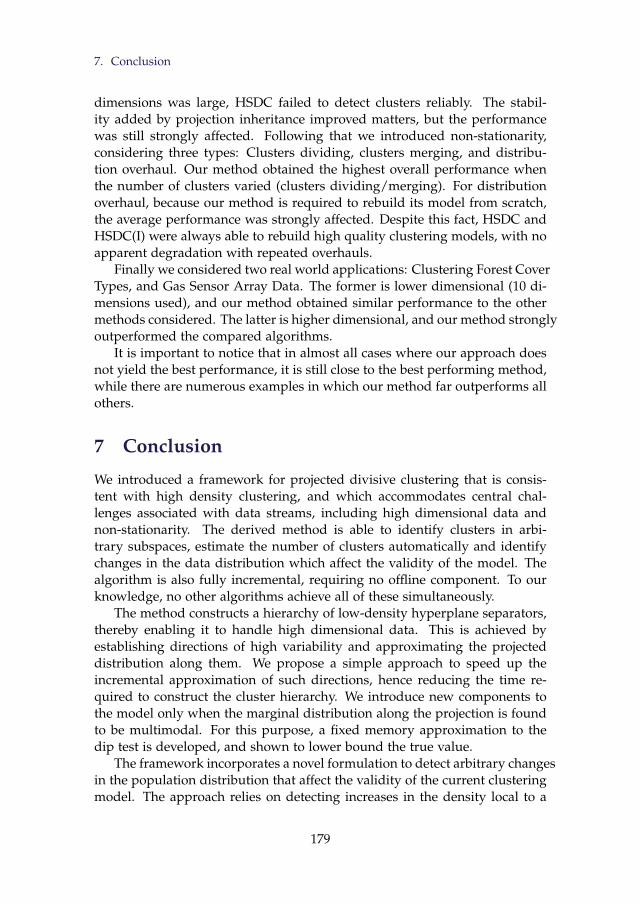
7. Conclusion
dimensions was large, HSDC failed to detect clusters reliably. The stabil-ity added by projection inheritance improved matters, but the performancewas still strongly affected. Following that we introduced non-stationarity,considering three types: Clusters dividing, clusters merging, and distribu-tion overhaul. Our method obtained the highest overall performance whenthe number of clusters varied (clusters dividing/merging). For distributionoverhaul, because our method is required to rebuild its model from scratch,the average performance was strongly affected. Despite this fact, HSDC andHSDC(I) were always able to rebuild high quality clustering models, with noapparent degradation with repeated overhauls.
Finally we considered two real world applications: Clustering Forest CoverTypes, and Gas Sensor Array Data. The former is lower dimensional (10 di-mensions used), and our method obtained similar performance to the othermethods considered. The latter is higher dimensional, and our method stronglyoutperformed the compared algorithms.
It is important to notice that in almost all cases where our approach doesnot yield the best performance, it is still close to the best performing method,while there are numerous examples in which our method far outperforms allothers.
7 Conclusion
We introduced a framework for projected divisive clustering that is consis-tent with high density clustering, and which accommodates central chal-lenges associated with data streams, including high dimensional data andnon-stationarity. The derived method is able to identify clusters in arbi-trary subspaces, estimate the number of clusters automatically and identifychanges in the data distribution which affect the validity of the model. Thealgorithm is also fully incremental, requiring no offline component. To ourknowledge, no other algorithms achieve all of these simultaneously.
The method constructs a hierarchy of low-density hyperplane separators,thereby enabling it to handle high dimensional data. This is achieved byestablishing directions of high variability and approximating the projecteddistribution along them. We propose a simple approach to speed up theincremental approximation of such directions, hence reducing the time re-quired to construct the cluster hierarchy. We introduce new components tothe model only when the marginal distribution along the projection is foundto be multimodal. For this purpose, a fixed memory approximation to thedip test is developed, and shown to lower bound the true value.
The framework incorporates a novel formulation to detect arbitrary changesin the population distribution that affect the validity of the current clusteringmodel. The approach relies on detecting increases in the density local to a
179
Chapter 5. Divisive Clustering of High Dimensional Data Streams
separating hyperplane, which signal that the hyperplane intersects regionsof high density. This enables us to not only provide indication of the timingof such changes but also to isolate the parts of the hierarchical model that re-quire revision. To our knowledge this is the first general purpose clusteringalgorithm able to detect changes in the underlying distribution.
Experimental results show that algorithms derived from the proposedframework obtain the best overall performance on a range of problem types,when compared with state of the art algorithms for data stream clustering.Among the competing methods, CluStream achieved an on-average betterperformance when the population distribution underwent the most extremetype of abrupt change. The reason is that reconstructing the entire cluster-ing hierarchy invariably requires more time than the adaptation of centroid-based methods. This result however is conditional on the a priori specifica-tion of the correct number of clusters for such algorithms. When this is notthe case our methods fare better.
Appendix. Proofs
Before we can prove Lemma 28, we require the following preliminaries.The algorithm for computing the dip of a distribution function F con-
structs a unimodal distribution function G with the following properties: (i)The modal interval of G, [m, M], is equal to the modal interval of the clos-est unimodal distribution function to F, which we denote by FU , based onthe supremum norm; (ii) ‖F−G‖∞ =2‖F−FU‖∞; (iii) G is the greatest con-vex minorant of F on (−∞,m]; (iv) G is the least concave majorant of F on[M,∞). By construction, the function G is linear between its nodes. A noden≤m of G satisfies G(n)= liminfx→n F(x), while a node n≥M of G satisfiesG(n)= limsupx→nF(x). If F is the distribution function of a discrete randomvariable, then G is continuous.
The function FU can be constructed by finding appropriate values b<m,B>M s.t. FU is equal to G+Dip(F) on [b,m], equal to G−Dip(F) on [M, B],linearly interpolating between G(m) and G(M) and given any appropriatetails, which we choose to be linearly decreasing/increasing to 0 and 1 respec-tively.
Before proving Lemma 28, we require the following preliminary result,which relies on the notion of a step linear function.
Step Linear A function f is step linear on a non-empty, compact interval I=[a,b], if
f (x)=α+β
⌊(x− a)
nb− a
⌋, ∀x∈ I,
for some α, β∈R and n∈N.
180
7. Conclusion
A step linear function is piecewise constant, and has n equally sized jumps ofsize β spaced equally on I with the final jump ocurring at b. The approximateempirical distribution function F (Section 4.2) is therefore step linear over theapproximating intervals.
Proposition 30 Let f be step linear on the closed interval I=[a,b], and satisfylimx→a− f (x)=α−β, where α, β as in the above definition for f . Let g be linear onI and continuous on a neighbourhood of I. Then
supx∈I| f (x)− g(x)|≤maxlimsupx→a| f (x)− g(x)|, limsupx→b| f (x)− g(x)| .
Proof Let fm and f M be linear on a neighbourhood of I s.t. they form the closestlower and upper bounding functions of f on I respectively. Since f is step linear, wehave,
limx→a−
f (x)= fm(a), limx→b− f (x)= fm(b),
f (a)= f M(a), f (b)= f M(b).
We therefore have, by above and the fact that g, fm, and f M are linear on I,
supx∈I| f (x)− g(x)|≤max
supx∈I| f M(x)− g(x)|, sup
x∈I| fm(x)− g(x)|
=max
| f M(b)− g(b)|, | f M(a)− g(a)|,
| fm(a)− g(a)|, | fm(b)− g(b)|=maxlimsupx→a| f (x)− g(x)|, limsupx→b| f (x)− g(x)| .
We are now in a position to prove Lemma 28, which states that the dip ofa compactly approximated sample, as described in Section 4.2, provides alower bound on the dip of the true sample.
Proof of Lemma 28.
Proof Let I=[a,b] be any compact interval and FI the empirical distributionfunction of (X ∩ Ic)∪Unif(X , I). Assume |X ∩ I|>1, since otherwise FI =FXand we are done. We can assume that the endpoints of I are elements ofX since this defines the same uniform set. FX and FI are therefore equalon Int(I)c. In fact, since X consists of unique points, ∃ε>0 s.t. FI(x)=FX (x) ∀x 6∈ (a+ε,b−ε). Define F′I to be equal to FU
X for x 6∈ Int(I) and linearlyinterpolating between FU
X (a) and FUX (b). By construction F′I is a continuous
unimodal distribution function.
181
Chapter 5. Divisive Clustering of High Dimensional Data Streams
We now show ‖FI−F′I‖∞≤‖FX −FUX ‖∞. To see this, suppose that it is not
true, i.e., ∃x s.t. |FI(x)−F′I(x)|>supy |FX (y)−FUX (y)|. Clearly x∈ Int(I) due
to the equalities discussed above and the construction of F′I . Because of thecontinuity of FU
X and F′I and the equality of FX and FI on (a, a+ε)∪ (b−ε,b),we have
limsupy→a|FI(y)−F′I(y)|= limsupy→a|FX −FUX (x)|
andlimsupy→b|FI(y)−F′I(y)|= limsupy→b|FX −FU
X (x)|.
But by Proposition 30 one of these left hand sides is at least as large as|FI(x)−F′I(x)|, leading to a contradiction.
We have shown that the addition of a single interval cannot increasethe dip. We can apply the same logic to the now modified sample (X ∩Ic)∪Unif(X , I), iterating the addition of disjoint intervals to obtain a non-increasing sequence of dips.
In the above proof, we do not show that F′I is the closest unimodal distri-bution function to FI , however its existence necessitates the closest one beingat least as close. Now, the sample approximations we employ still contain afull t atoms after t observations, however, they can be stored in O(k) for kintervals. We can easily show that the dip of such a sample approximationcan be computed in O(k) time.
Proposition 31 The dip of a sample consisting of k uniform sets with disjoint rangescan be computed in O(k) time.
Proof We begin by showing that there exists a unimodal distribution functionwhich is linear on the ranges of the uniform sets and which achieves theminimal distance to the empirical distribution function of the sample.
Let F be a continuous unimodal distribution function s.t. ‖F− F‖∞ =Dip(F). Define F′ similarly to in the above proof to be the continuous dis-tribution function which is equal to F outside and at the boundaries of theintervals defining the uniform sets and linearly interpolating on them. Usingthe same logic, we know that supx |F′(x)− F(x)|≤supx |F(x)− F(x)|, hence‖F′− F‖∞ =Dip(F).
Proposition 30 ensures that points in the interior of the intervals will notbe chosen by the dip algorithm as end points of the modal interval of G,nor points at which the difference between the functions is supremal. Thepossible choices for these locations is therefore O(k), and the algorithm neednot evaluate the functions except at the endpoints of the intervals.
Finally, we provide a proof of Proposition 29.
182
7. Conclusion
Proof of Proposition 29.
Proof For s>1 we have
‖vs−vs−1‖=‖vs‖‖vs−vs−1‖≥|vs · (vs−vs−1)|= |vsvs−1−1|,
since ‖vt‖=1 ∀t. Therefore, since vt∞t=1 is almost surely convergent, and
therefore almost surely Cauchy, we have vs ·vs−1a.s.−→1⇒arccos(vs ·vs−1)
a.s.−→0. Now, we can easily show that,
λt≤γt−1λ1+(1−γ)t−2
∑i=1
γi arccos(vt−i ·vt−i−1).
Take ε>0 and t large enough that γt−1λ1<γε, and t> k+2, where k=blog(ε(1−γ)/2π)/log(γ)−1c. Consider,
t−2
∑i=1
γi arccos(vt−i ·vt−i−1)≤k
∑i=1
arccos(vt−i ·vt−i−1)+πγk+1
1−γ,
and πγk+1
1−γ ≤ε2 . In all,
λt >ε⇒k
∑i=0
arccos(vt−i ·vt−i−1)>ε/2.
Notice that k does not depend on t. With probability 1, for any given ε>0there is a T s.t. T>T implies ∑k
i=0 arccos(vT−i ·vT−i−1)≤ε/2, implying λT≤ε for all T>T , and the result follows.
Acknowledgements
David Hofmeyr gratefully acknowledges funding from both the Engineer-ing and Physical Sciences Research Council (EPSRC) and the OppenheimerMemorial Trust.
183
Chapter 6
Conclusion
1 Summary of Contributions
This thesis consists of four new approaches to the important problem of iden-tifying groups, or clusters of related data, which has applications in all areasof scientific research from robotics to microarray analysis to marketing strat-egy and many more. The contributions are motivated by two fundamentalchallenges in the context of data clustering, dimension reduction and to alesser extent data streams. The problem of dimension reduction is treated ina highly principled manner, by identifying subspaces in which the data rep-resent a clusterable structure in relation to fundamental definitions of cluster.The combination of high dimensionality and sequential arrival of data, as ina data stream, is handled by integrating the tasks of dimension reduction andincremental learning which allows for some of the main difficulties in datastreams to be tackled effectively.
In Chapter 2 a new hyperplane based classifier is proposed for unsuper-vised and semi-supervised classification. The optimal hyperplane is definedas that which has the minimum integrated density along it, while induc-ing a meaningful partition of a data set. This approach is motivated by thewidely regarded low density separation assumption; (high density) clustersare regions of relatively high density separated by low density regions. Themajority of existing approaches which are based on this assumption attemptto find the hyperplane which has the largest margin on the data set, whichis at best asymptotically connected with the actual lowest density separator.The proposed approach directly estimates the density using kernel densityestimation, and so has a much more pleasing interpretation in the finite sam-ple setting. It is apparent that no other existing methods have attempted tosolve the low density separation problem directly in the finite sample setting.
184
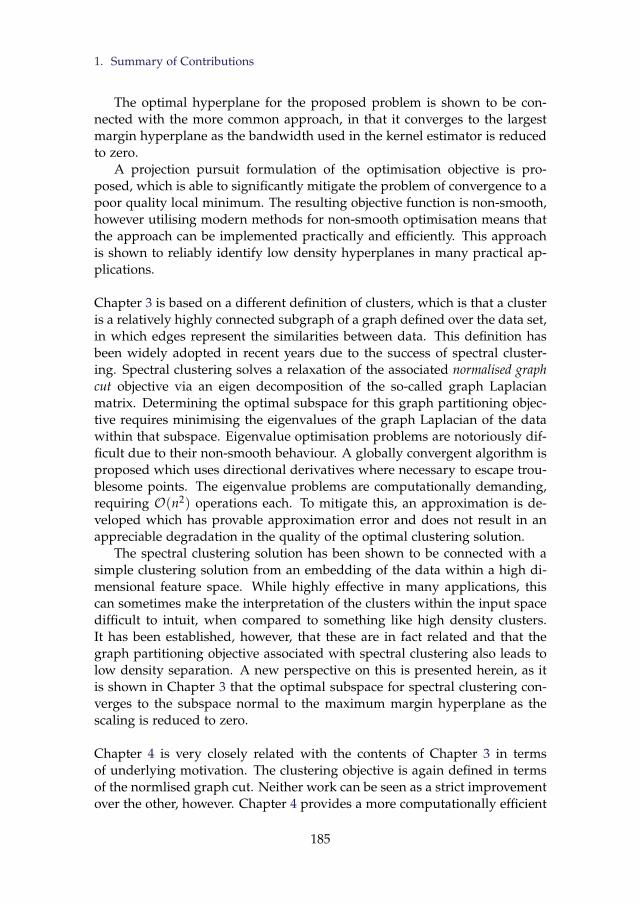
1. Summary of Contributions
The optimal hyperplane for the proposed problem is shown to be con-nected with the more common approach, in that it converges to the largestmargin hyperplane as the bandwidth used in the kernel estimator is reducedto zero.
A projection pursuit formulation of the optimisation objective is pro-posed, which is able to significantly mitigate the problem of convergence to apoor quality local minimum. The resulting objective function is non-smooth,however utilising modern methods for non-smooth optimisation means thatthe approach can be implemented practically and efficiently. This approachis shown to reliably identify low density hyperplanes in many practical ap-plications.
Chapter 3 is based on a different definition of clusters, which is that a clusteris a relatively highly connected subgraph of a graph defined over the data set,in which edges represent the similarities between data. This definition hasbeen widely adopted in recent years due to the success of spectral cluster-ing. Spectral clustering solves a relaxation of the associated normalised graphcut objective via an eigen decomposition of the so-called graph Laplacianmatrix. Determining the optimal subspace for this graph partitioning objec-tive requires minimising the eigenvalues of the graph Laplacian of the datawithin that subspace. Eigenvalue optimisation problems are notoriously dif-ficult due to their non-smooth behaviour. A globally convergent algorithm isproposed which uses directional derivatives where necessary to escape trou-blesome points. The eigenvalue problems are computationally demanding,requiring O(n2) operations each. To mitigate this, an approximation is de-veloped which has provable approximation error and does not result in anappreciable degradation in the quality of the optimal clustering solution.
The spectral clustering solution has been shown to be connected with asimple clustering solution from an embedding of the data within a high di-mensional feature space. While highly effective in many applications, thiscan sometimes make the interpretation of the clusters within the input spacedifficult to intuit, when compared to something like high density clusters.It has been established, however, that these are in fact related and that thegraph partitioning objective associated with spectral clustering also leads tolow density separation. A new perspective on this is presented herein, as itis shown in Chapter 3 that the optimal subspace for spectral clustering con-verges to the subspace normal to the maximum margin hyperplane as thescaling is reduced to zero.
Chapter 4 is very closely related with the contents of Chapter 3 in termsof underlying motivation. The clustering objective is again defined in termsof the normlised graph cut. Neither work can be seen as a strict improvementover the other, however. Chapter 4 provides a more computationally efficient
185
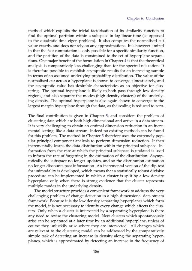
Chapter 6. Conclusion
method which exploits the trivial factorisation of its similarity function tofind the optimal partition within a subspace in log-linear time (as opposedto the quadratic time eigen problem). It also computes the normalised cutvalue exactly, and does not rely on any approximations. It is however limitedin that the fast computation is only possible for a specific similarity function,and the partition of the data is constrained to the set of hyperplane separa-tions. One major benefit of the formulation in Chapter 4 is that the theoreticalanalysis is comparatively less challenging than for the spectral relaxation. Itis therefore possible to establish asymptotic results for an increasing samplein terms of an assumed underlying probability distribution. The value of thenormalised cut across a hyperplane is shown to converge almost surely, andthe asymptotic value has desirable characteristics as an objective for clus-tering. The optimal hyperplane is likely to both pass through low densityregions, and also separate the modes (high density clusters) of the underly-ing density. The optimal hyperplane is also again shown to converge to thelargest margin hyperplane through the data, as the scaling is reduced to zero.
The final contribution is given in Chapter 5, and considers the problem ofclustering data which are both high dimensional and arrive in a data stream.It is very challenging to obtain an optimal dimension reduction in an incre-mental setting, like a data stream. Indeed no existing methods can be foundfor this problem. The method in Chapter 5 therefore uses the extremely pop-ular principal component analysis to perform dimension reduction. It thenincrementally learns the data distribution within the principal subspace. In-formation from the rate at which the principal subspace is updated is usedto inform the rate of forgetting in the estimation of the distribution. Asymp-totically the subspace no longer updates, and so the distribution estimationno longer discounts past information. An incremental version of the dip testfor unimodality is developed, which means that a statistically robust divisiveprocedure can be implemented in which a cluster is split by a low densityhyperplane only when there is strong evidence that the cluster representsmultiple modes in the underlying density.
The model structure provides a convenient framework to address the verychallenging problem of change detection in a high dimensional data streamframework. Because it is the low density separating hyperplanes which formthe model, it is not necessary to identify every change which affects the clus-ters. Only when a cluster is intersected by a separating hyperplane is thereany need to revise the clustering model. New clusters which spontaneouslyarise can be separated at a later time by an additional hyperplane, unless ofcourse they unluckily arise where they are intersected. All changes whichare relevant to the clustering model can be addressed by the comparativelysimple task of detecting an increase in density along the separating hyper-planes, which is approximated by detecting an increase in the frequency of
186
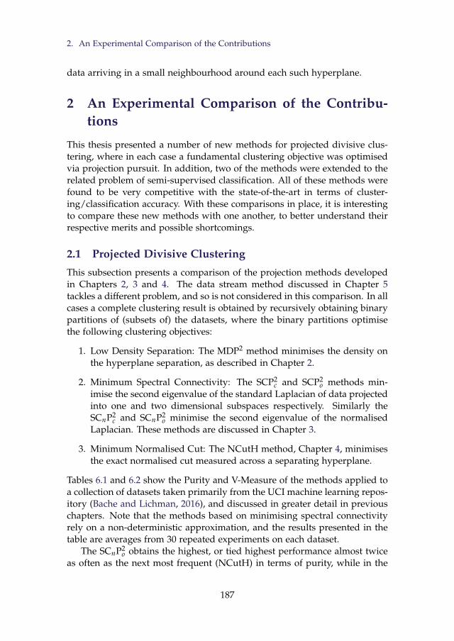
2. An Experimental Comparison of the Contributions
data arriving in a small neighbourhood around each such hyperplane.
2 An Experimental Comparison of the Contribu-tions
This thesis presented a number of new methods for projected divisive clus-tering, where in each case a fundamental clustering objective was optimisedvia projection pursuit. In addition, two of the methods were extended to therelated problem of semi-supervised classification. All of these methods werefound to be very competitive with the state-of-the-art in terms of cluster-ing/classification accuracy. With these comparisons in place, it is interestingto compare these new methods with one another, to better understand theirrespective merits and possible shortcomings.
2.1 Projected Divisive Clustering
This subsection presents a comparison of the projection methods developedin Chapters 2, 3 and 4. The data stream method discussed in Chapter 5tackles a different problem, and so is not considered in this comparison. In allcases a complete clustering result is obtained by recursively obtaining binarypartitions of (subsets of) the datasets, where the binary partitions optimisethe following clustering objectives:
1. Low Density Separation: The MDP2 method minimises the density onthe hyperplane separation, as described in Chapter 2.
2. Minimum Spectral Connectivity: The SCP2c and SCP2
o methods min-imise the second eigenvalue of the standard Laplacian of data projectedinto one and two dimensional subspaces respectively. Similarly theSCnP2
c and SCnP2o minimise the second eigenvalue of the normalised
Laplacian. These methods are discussed in Chapter 3.
3. Minimum Normalised Cut: The NCutH method, Chapter 4, minimisesthe exact normalised cut measured across a separating hyperplane.
Tables 6.1 and 6.2 show the Purity and V-Measure of the methods applied toa collection of datasets taken primarily from the UCI machine learning repos-itory (Bache and Lichman, 2016), and discussed in greater detail in previouschapters. Note that the methods based on minimising spectral connectivityrely on a non-deterministic approximation, and the results presented in thetable are averages from 30 repeated experiments on each dataset.
The SCnP2o obtains the highest, or tied highest performance almost twice
as often as the next most frequent (NCutH) in terms of purity, while in the
187
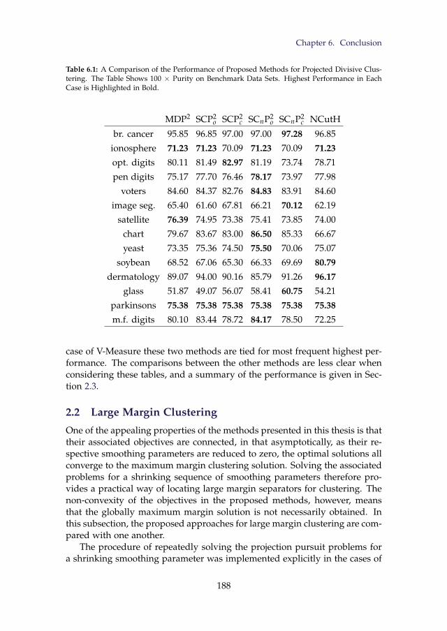
Chapter 6. Conclusion
Table 6.1: A Comparison of the Performance of Proposed Methods for Projected Divisive Clus-tering. The Table Shows 100 × Purity on Benchmark Data Sets. Highest Performance in EachCase is Highlighted in Bold.
MDP2 SCP2o SCP2
c SCnP2o SCnP2
c NCutH
br. cancer 95.85 96.85 97.00 97.00 97.28 96.85
ionosphere 71.23 71.23 70.09 71.23 70.09 71.23opt. digits 80.11 81.49 82.97 81.19 73.74 78.71
pen digits 75.17 77.70 76.46 78.17 73.97 77.98
voters 84.60 84.37 82.76 84.83 83.91 84.60
image seg. 65.40 61.60 67.81 66.21 70.12 62.19
satellite 76.39 74.95 73.38 75.41 73.85 74.00
chart 79.67 83.67 83.00 86.50 85.33 66.67
yeast 73.35 75.36 74.50 75.50 70.06 75.07
soybean 68.52 67.06 65.30 66.33 69.69 80.79dermatology 89.07 94.00 90.16 85.79 91.26 96.17
glass 51.87 49.07 56.07 58.41 60.75 54.21
parkinsons 75.38 75.38 75.38 75.38 75.38 75.38m.f. digits 80.10 83.44 78.72 84.17 78.50 72.25
case of V-Measure these two methods are tied for most frequent highest per-formance. The comparisons between the other methods are less clear whenconsidering these tables, and a summary of the performance is given in Sec-tion 2.3.
2.2 Large Margin Clustering
One of the appealing properties of the methods presented in this thesis is thattheir associated objectives are connected, in that asymptotically, as their re-spective smoothing parameters are reduced to zero, the optimal solutions allconverge to the maximum margin clustering solution. Solving the associatedproblems for a shrinking sequence of smoothing parameters therefore pro-vides a practical way of locating large margin separators for clustering. Thenon-convexity of the objectives in the proposed methods, however, meansthat the globally maximum margin solution is not necessarily obtained. Inthis subsection, the proposed approaches for large margin clustering are com-pared with one another.
The procedure of repeatedly solving the projection pursuit problems fora shrinking smoothing parameter was implemented explicitly in the cases of
188
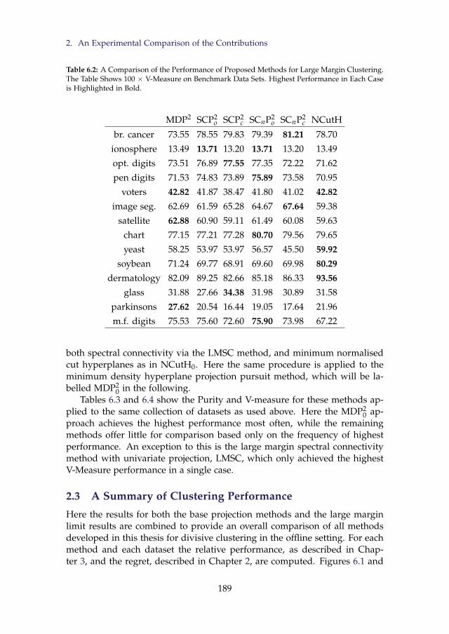
2. An Experimental Comparison of the Contributions
Table 6.2: A Comparison of the Performance of Proposed Methods for Large Margin Clustering.The Table Shows 100 × V-Measure on Benchmark Data Sets. Highest Performance in Each Caseis Highlighted in Bold.
MDP2 SCP2o SCP2
c SCnP2o SCnP2
c NCutH
br. cancer 73.55 78.55 79.83 79.39 81.21 78.70
ionosphere 13.49 13.71 13.20 13.71 13.20 13.49
opt. digits 73.51 76.89 77.55 77.35 72.22 71.62
pen digits 71.53 74.83 73.89 75.89 73.58 70.95
voters 42.82 41.87 38.47 41.80 41.02 42.82image seg. 62.69 61.59 65.28 64.67 67.64 59.38
satellite 62.88 60.90 59.11 61.49 60.08 59.63
chart 77.15 77.21 77.28 80.70 79.56 79.65
yeast 58.25 53.97 53.97 56.57 45.50 59.92soybean 71.24 69.77 68.91 69.60 69.98 80.29
dermatology 82.09 89.25 82.66 85.18 86.33 93.56glass 31.88 27.66 34.38 31.98 30.89 31.58
parkinsons 27.62 20.54 16.44 19.05 17.64 21.96
m.f. digits 75.53 75.60 72.60 75.90 73.98 67.22
both spectral connectivity via the LMSC method, and minimum normalisedcut hyperplanes as in NCutH0. Here the same procedure is applied to theminimum density hyperplane projection pursuit method, which will be la-belled MDP2
0 in the following.Tables 6.3 and 6.4 show the Purity and V-measure for these methods ap-
plied to the same collection of datasets as used above. Here the MDP20 ap-
proach achieves the highest performance most often, while the remainingmethods offer little for comparison based only on the frequency of highestperformance. An exception to this is the large margin spectral connectivitymethod with univariate projection, LMSC, which only achieved the highestV-Measure performance in a single case.
2.3 A Summary of Clustering Performance
Here the results for both the base projection methods and the large marginlimit results are combined to provide an overall comparison of all methodsdeveloped in this thesis for divisive clustering in the offline setting. For eachmethod and each dataset the relative performance, as described in Chap-ter 3, and the regret, described in Chapter 2, are computed. Figures 6.1 and
189
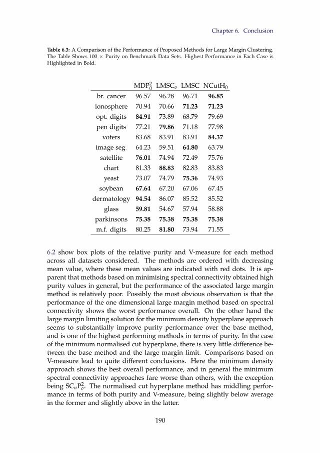
Chapter 6. Conclusion
Table 6.3: A Comparison of the Performance of Proposed Methods for Large Margin Clustering.The Table Shows 100 × Purity on Benchmark Data Sets. Highest Performance in Each Case isHighlighted in Bold.
MDP20 LMSCo LMSC NCutH0
br. cancer 96.57 96.28 96.71 96.85ionosphere 70.94 70.66 71.23 71.23opt. digits 84.91 73.89 68.79 79.69
pen digits 77.21 79.86 71.18 77.98
voters 83.68 83.91 83.91 84.37image seg. 64.23 59.51 64.80 63.79
satellite 76.01 74.94 72.49 75.76
chart 81.33 88.83 82.83 83.83
yeast 73.07 74.79 75.36 74.93
soybean 67.64 67.20 67.06 67.45
dermatology 94.54 86.07 85.52 85.52
glass 59.81 54.67 57.94 58.88
parkinsons 75.38 75.38 75.38 75.38m.f. digits 80.25 81.80 73.94 71.55
6.2 show box plots of the relative purity and V-measure for each methodacross all datasets considered. The methods are ordered with decreasingmean value, where these mean values are indicated with red dots. It is ap-parent that methods based on minimising spectral connectivity obtained highpurity values in general, but the performance of the associated large marginmethod is relatively poor. Possibly the most obvious observation is that theperformance of the one dimensional large margin method based on spectralconnectivity shows the worst performance overall. On the other hand thelarge margin limiting solution for the minimum density hyperplane approachseems to substantially improve purity performance over the base method,and is one of the highest performing methods in terms of purity. In the caseof the minimum normalised cut hyperplane, there is very little difference be-tween the base method and the large margin limit. Comparisons based onV-measure lead to quite different conclusions. Here the minimum densityapproach shows the best overall performance, and in general the minimumspectral connectivity approaches fare worse than others, with the exceptionbeing SCnP2
o . The normalised cut hyperplane method has middling perfor-mance in terms of both purity and V-measure, being slightly below averagein the former and slightly above in the latter.
190
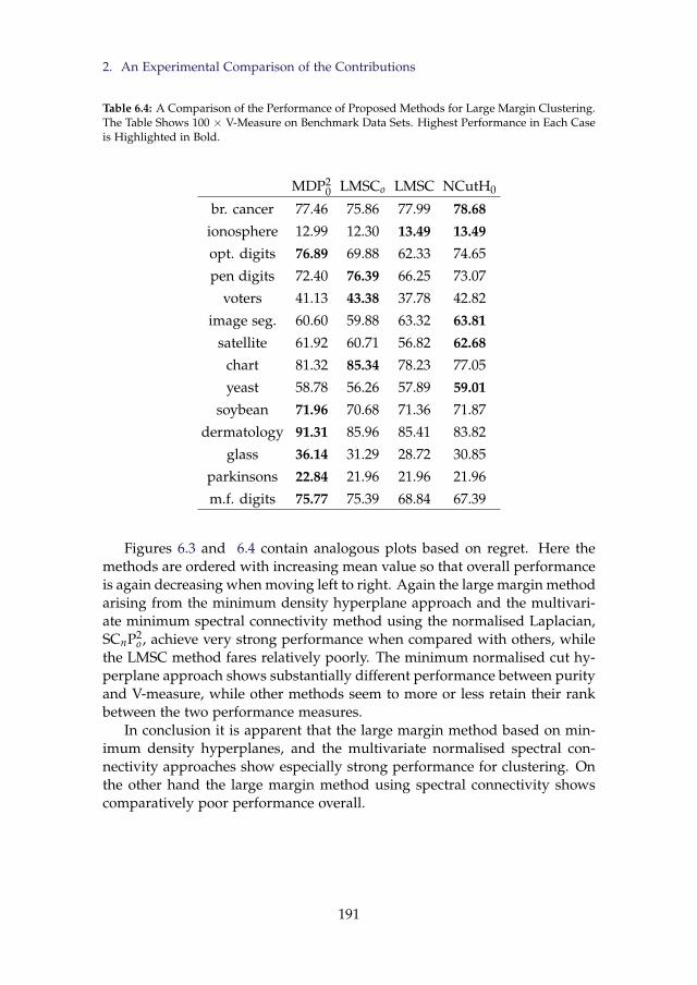
2. An Experimental Comparison of the Contributions
Table 6.4: A Comparison of the Performance of Proposed Methods for Large Margin Clustering.The Table Shows 100 × V-Measure on Benchmark Data Sets. Highest Performance in Each Caseis Highlighted in Bold.
MDP20 LMSCo LMSC NCutH0
br. cancer 77.46 75.86 77.99 78.68ionosphere 12.99 12.30 13.49 13.49opt. digits 76.89 69.88 62.33 74.65
pen digits 72.40 76.39 66.25 73.07
voters 41.13 43.38 37.78 42.82
image seg. 60.60 59.88 63.32 63.81satellite 61.92 60.71 56.82 62.68
chart 81.32 85.34 78.23 77.05
yeast 58.78 56.26 57.89 59.01soybean 71.96 70.68 71.36 71.87
dermatology 91.31 85.96 85.41 83.82
glass 36.14 31.29 28.72 30.85
parkinsons 22.84 21.96 21.96 21.96
m.f. digits 75.77 75.39 68.84 67.39
Figures 6.3 and 6.4 contain analogous plots based on regret. Here themethods are ordered with increasing mean value so that overall performanceis again decreasing when moving left to right. Again the large margin methodarising from the minimum density hyperplane approach and the multivari-ate minimum spectral connectivity method using the normalised Laplacian,SCnP2
o , achieve very strong performance when compared with others, whilethe LMSC method fares relatively poorly. The minimum normalised cut hy-perplane approach shows substantially different performance between purityand V-measure, while other methods seem to more or less retain their rankbetween the two performance measures.
In conclusion it is apparent that the large margin method based on min-imum density hyperplanes, and the multivariate normalised spectral con-nectivity approaches show especially strong performance for clustering. Onthe other hand the large margin method using spectral connectivity showscomparatively poor performance overall.
191
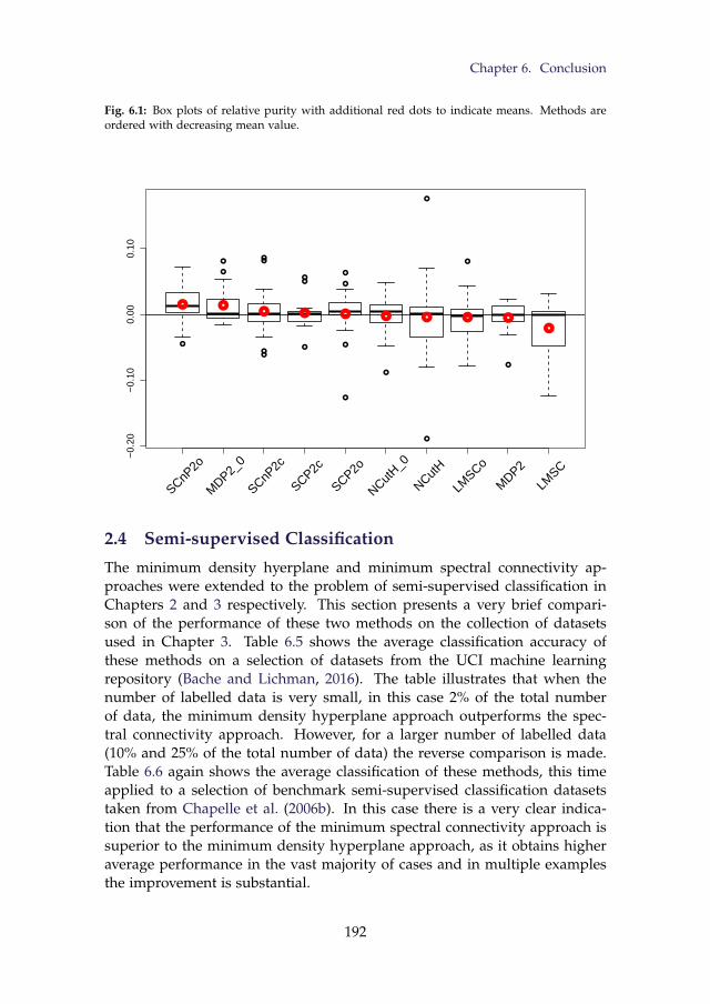
Chapter 6. Conclusion
Fig. 6.1: Box plots of relative purity with additional red dots to indicate means. Methods areordered with decreasing mean value.
−0.
20−
0.10
0.00
0.10
SCnP2o
MDP2_
0
SCnP2c
SCP2c
SCP2o
NCutH_0
NCutH
LMSCo
MDP2
LMSC
2.4 Semi-supervised Classification
The minimum density hyerplane and minimum spectral connectivity ap-proaches were extended to the problem of semi-supervised classification inChapters 2 and 3 respectively. This section presents a very brief compari-son of the performance of these two methods on the collection of datasetsused in Chapter 3. Table 6.5 shows the average classification accuracy ofthese methods on a selection of datasets from the UCI machine learningrepository (Bache and Lichman, 2016). The table illustrates that when thenumber of labelled data is very small, in this case 2% of the total numberof data, the minimum density hyperplane approach outperforms the spec-tral connectivity approach. However, for a larger number of labelled data(10% and 25% of the total number of data) the reverse comparison is made.Table 6.6 again shows the average classification of these methods, this timeapplied to a selection of benchmark semi-supervised classification datasetstaken from Chapelle et al. (2006b). In this case there is a very clear indica-tion that the performance of the minimum spectral connectivity approach issuperior to the minimum density hyperplane approach, as it obtains higheraverage performance in the vast majority of cases and in multiple examplesthe improvement is substantial.
192
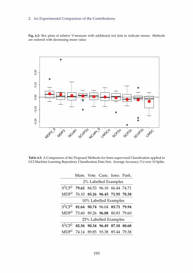
2. An Experimental Comparison of the Contributions
Fig. 6.2: Box plots of relative V-measure with additional red dots to indicate means. Methodsare ordered with decreasing mean value.
−0.
20−
0.10
0.00
0.10
0.20
MDP2_
0
MDP2
NCutH
SCnP2o
NCutH_0
LMSCo
SCP2o
SCP2c
SCnP2c
LMSC
Table 6.5: A Comparison of the Proposed Methods for Semi-supervised Classification applied toUCI Machine Learning Repository Classification Data Sets. Average Accuracy (%) over 10 Splits.
Mam. Vote. Canc. Iono. Park.
2% Labelled Examples
S3CP2 79.62 84.53 96.18 66.44 74.71
MDP2 76.10 85.26 96.45 71.95 78.38
10% Labelled Examples
S3CP2 81.64 90.74 96.04 85.71 79.94MDP2 73.60 89.26 96.08 80.83 79.60
25% Labelled Examples
S3CP2 82.54 90.34 96.49 87.18 80.68MDP2 74.14 89.85 93.38 85.44 79.38
193
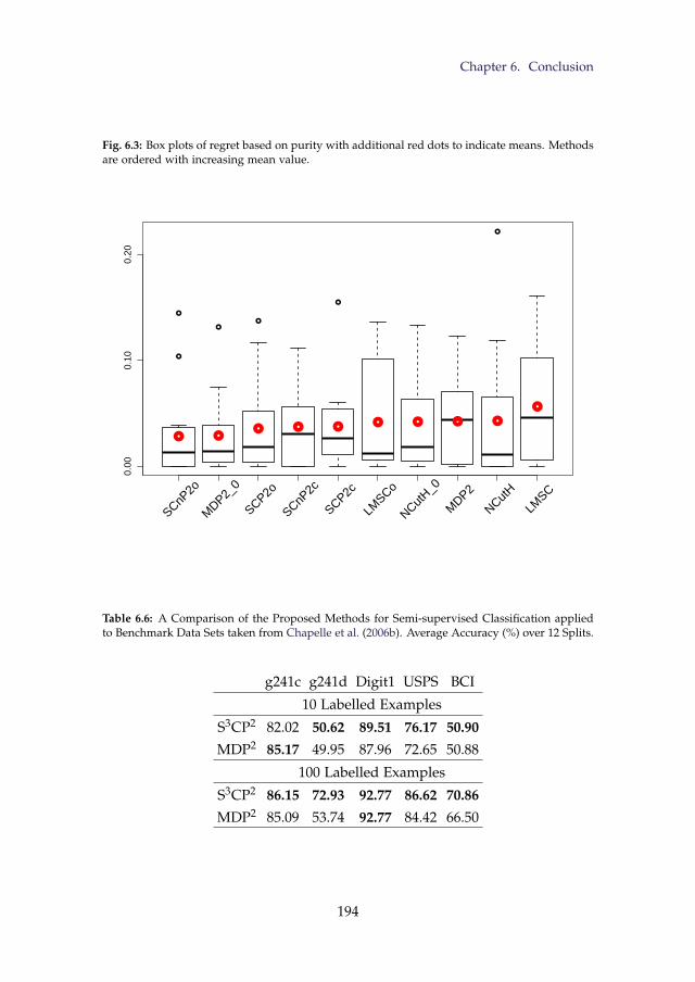
Chapter 6. Conclusion
Fig. 6.3: Box plots of regret based on purity with additional red dots to indicate means. Methodsare ordered with increasing mean value.
0.00
0.10
0.20
SCnP2o
MDP2_
0
SCP2o
SCnP2c
SCP2c
LMSCo
NCutH_0
MDP2
NCutH
LMSC
Table 6.6: A Comparison of the Proposed Methods for Semi-supervised Classification appliedto Benchmark Data Sets taken from Chapelle et al. (2006b). Average Accuracy (%) over 12 Splits.
g241c g241d Digit1 USPS BCI
10 Labelled Examples
S3CP2 82.02 50.62 89.51 76.17 50.90MDP2 85.17 49.95 87.96 72.65 50.88
100 Labelled Examples
S3CP2 86.15 72.93 92.77 86.62 70.86MDP2 85.09 53.74 92.77 84.42 66.50
194
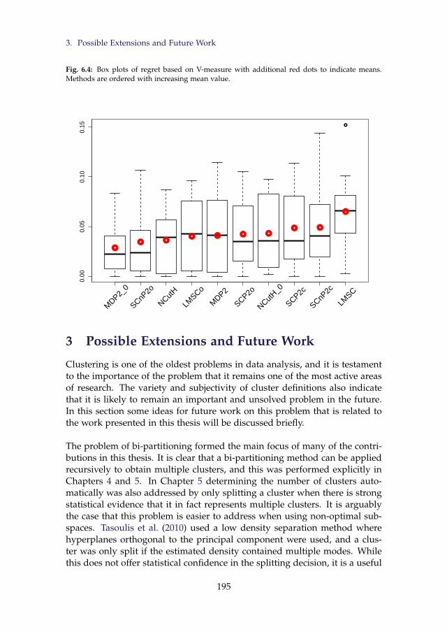
3. Possible Extensions and Future Work
Fig. 6.4: Box plots of regret based on V-measure with additional red dots to indicate means.Methods are ordered with increasing mean value.
0.00
0.05
0.10
0.15
MDP2_
0
SCnP2o
NCutH
LMSCo
MDP2
SCP2o
NCutH_0
SCP2c
SCnP2c
LMSC
3 Possible Extensions and Future Work
Clustering is one of the oldest problems in data analysis, and it is testamentto the importance of the problem that it remains one of the most active areasof research. The variety and subjectivity of cluster definitions also indicatethat it is likely to remain an important and unsolved problem in the future.In this section some ideas for future work on this problem that is related tothe work presented in this thesis will be discussed briefly.
The problem of bi-partitioning formed the main focus of many of the contri-butions in this thesis. It is clear that a bi-partitioning method can be appliedrecursively to obtain multiple clusters, and this was performed explicitly inChapters 4 and 5. In Chapter 5 determining the number of clusters auto-matically was also addressed by only splitting a cluster when there is strongstatistical evidence that it in fact represents multiple clusters. It is arguablythe case that this problem is easier to address when using non-optimal sub-spaces. Tasoulis et al. (2010) used a low density separation method wherehyperplanes orthogonal to the principal component were used, and a clus-ter was only split if the estimated density contained multiple modes. Whilethis does not offer statistical confidence in the splitting decision, it is a useful
195
Chapter 6. Conclusion
heuristic.The principal challenge when looking at optimal subspaces becomes ap-
parent in the extreme case where the number of dimensions is greater thanthe number of data. If there are n data in d>n dimensions and the data arestored in a matrix X ∈Rn×d, then the projection equation given by X v= p hasinfinitely many solutions v for any vector p∈Rn, provided there are at leastn linearly independent dimensions in the data set. What this means is thatregardless of the actual cluster structure in the data, there is a subspace inwhich they can be made to look like any equally weighted discrete distribu-tion with n atoms, up to a scaling constant. For example, for any bi-partitionof the data set, each subset can be projected to a single point, making thedata set in some sense maximally clusterable for any bi-partition.
So called L1 regularisation has been used for problems like regression inhigh dimensional applications (Tibshirani, 1996). A regularisation of projec-tion pursuit seems a natural way to overcome the above problem, but thisadds to the difficulty in establishing when there is statistical confidence thata cluster should be split.
It would be very interesting to both establish robust rules for determin-ing the presence of multiple clusters for the proposed methods, and also toinvestigate how regularisations affect the number of degrees of freedom inthe resulting solution so that these can be usefully implemented in higherdimensional examples.
In recent years the high dimensionality problem has entered the realms of“Big Data". When the number of dimensions is so large that only a few datapoints can be stored in a computer’s memory it is not possible to processthe data in their original form. Random projections have become the go-toapproach for dealing with these types of data. The popular result of Johnsonand Lindenstrauss (1984) places a probabilistic bound on the error inducedby random projections on the structure of the data. This result has beenextended such that the error of a clustering model acting on the randomlyprojected data, rather than the original data set, can be evaluated (Boutsidiset al., 2010; Tasoulis et al., 2013).
An interesting observation made by a number of authors is that data aris-ing from multiple clusters, when projected into a random subspace, tend toappear as a mixture of Gaussians (Dasgupta, 2000; Fern and Brodley, 2003;Tasoulis et al., 2013). Theoretical investigations into the properties of randomprojections have shown that under certain conditions, asymptotically as thenumber of dimensions tends to infinity, almost all projections of a data setare Gaussian (Noar and Romik, 2003; Dasgupta et al., 2006). What may behappening in the case of multiple clusters is that the convergence to Gaus-sianity within the clusters occurs at a faster rate than globally over the wholedata set, due to their being somewhat closer to Gaussian to begin with. For
196
3. Possible Extensions and Future Work
finitely many dimensions, but large enough to observe the convergence toGaussianity within clusters, one therefore observes a mixture of Gaussians.
The size of the random subspace dictated by Johnson and Lindenstrauss(1984) is often still large enough that further dimension reduction is neces-sary to render meaningful results. Using the observation of Dasgupta et al.(2006) may offer an assumption that the data are close to a mixture of Gaus-sians. A projection pursuit based on optimally separating a Gaussian mixtureshould therefore offer a promising method for learning the optimal subspacein which to perform clustering.
As a final idea, the data stream setting is revisited. In the last section aremark was made about the infeasibility of finding optimal projections in thedata stream setting. This does not, however, preclude an attempt to find lo-cally optimal hyperplane separators. Returning to the assumption that highdensity clusters can be separated by low density regions, it may be possibleto find locally minimum density hyperplanes in a fully incremental way.
Optimisation with sequential access to data is very often addressed usingstochastic gradient descent (Bottou, 2010). When a noisy estimate of the gra-dient of the objective function can be observed with each arriving data point,then moving along the negative of these gradients for an appropriately sizedsequence of steps leads to convergence to a local minimum in the objective.The bias in the gradient of a kernel based estimate of a probability density isindependent of the number of data used in the estimate. The size of the biasis, in fact, controlled by the size of the bandwidth. Repeatedly updating ahyperplane by moving along the negative of the gradient of a kernel locatedon the most recently observed datum will decrease the density along the hy-perplane. Some important caveats exist, however. Firstly, the density tendsto zero in the tails of the distribution, and so if the hyperplane escapes theconvex hull of the modes of the density then it will not converge. To avoidthis problem, a simple bounding method can be used which prevents thehyperplane from deviating too far from the mean of the data. Alternatively,it may be possible to estimate the modes of the density in a similar mannerto decreasing the density on a hyperplane, and thereby force the hyperplaneto intersect their convex hull. Secondly, though the bias can be controlledby allowing the bandwidth to tend to zero, this has the effect of inflatingthe variance of the gradient estimates. This is a similar problem to that ob-served in the algorithm of Kiefer and Wolfowitz (1952). It may be possibleto define a sequence of step sizes such that both the bias and the variancein the updates tend to zero asymptotically, in which case convergence canbe achieved. Alternatively, a small but non-zero bandwidth can be used oncesufficiently many data have been observed, which means that the hyperplanewill not necessarily converge to a local minimum but the variance in the up-date equation is guaranteed to be well controlled.
197
Bibliography
Ackerman, M. and Ben David, S. Clusterability: A Theoretical Study. In Pro-ceedings of AISTATS, JMLR: W&CP, 5:1-8, 2009.
Aggarwal, C. C., Procopiuc, C. M., Wolf, J. L., Yu, P. S. and Park, J. S. Fastalgorithms for projected clustering. In Proceedings of the ACM InternationalConference on Management of Data, 1999.
Aggarwal, C. C. and Yu, P. S. Finding generalized projected clusters in highdimensional space. In Proceedings of the ACM International Conference onManagement of Data, 2000.
Aggarwal, C. C., Hinneburg, A., and Keim, D. On the surprising behavior ofdistance metrics in high dimensional space. In Proceedings of the 8th Interna-tional Conference on Database Theory, 2001.
Aggarwal, C. C.: A survey of stream clustering algorithms. Data Clustering:Algorithms and Applications, Aggarwal C. C., Reddy C. (eds.), 457-482, 2013.
Aggarwal, C. C., and Reddy, C. K. Data Clustering: Algorithms and Applications.CRC Press, 2013.
Aggarwal, C. C., Han, J., Wang, J., Yu, P.: A framework for clustering evolvingdata streams. Proceedings of the 29th international conference on Very large databases. 29, 81-92, 2003.
Aggarwal, C. C., Han, J., Wang, J., Yu, P. S.: A framework for projectedclustering of high dimensional data streams. Proceedings of the Thirtieth in-ternational conference on Very large data bases. 852-863, 2004.
Agrawal, R., Gehrke, J., Gunopulos, D. and Raghavan, P. Automatic subspaceclustering of high dimensional data for data mining applications. In Pro-ceedings of the ACM International Conference on Management of Data, 1998.
E. Aitnouri, S. Wang, and D. Ziou. On comparison of clustering techniquesfor histogram pdf estimation. Pattern Recognition and Image Analysis, 10(2):206–217, 2000.
198
3. Possible Extensions and Future Work
Allgower, E. L. and Georg, K. Numerical continuation methods: an introduction,Volume 13. Springer Science & Business Media, 2012.
Amini, A., Saboohi, H., Wah, T.Y., Herawan, T.: Dmm-stream: A densitymini-micro clustering algorithm for evolving datastreams. In Proceedings ofthe First International Conference on Advanced Data and Information Engineer-ing, 675-682, 2014.
Amini, A., Wah, T.Y., Saboohi, H.: On density based data streams clusteringalgorithms: A survey. Journal of Computer Science and Technology, 29(1) 116-141, 2014.
Anagnostopoulos, C., Tasoulis, D. K., Adams, N. M., Pavlidis, N. G., Hand,D. J.: Online linear and quadratic discriminant analysis with adaptive for-getting for streaming classification. Statistical Analysis and Data Mining. 5(2),139-166, 2012.
Ankerst, M., Breunig, M., Kriegel, H.P., Sander, J.: OPTICS: ordering points toidentify the clustering structure. Proceedings of the ACM Sigmod Conference.49-60, 1999.
Artac, M., Jogan, M., Leonardis, A.: Incremental PCA for on-line visual learn-ing and recognition. Proceedings of the 16th International Conference on PatternRecognition. 3, 781-784, 2002.
D. Arthur and S. Vassilvitskii. k-means++: The advantages of careful seeding.In Proceedings of the Eighteenth Annual ACM-SIAM Symposium on DiscreteAlgorithms, SODA ’07, pages 1027–1035, 2007.
Azzalini, A. and Torelli, N. Clustering via nonparametric density estimation.Statistics and Computing, 17(1):71–80, 2007.
Babcock, B., Babu, S., Datar, M., Motwani, R., Widom, J.: Models and issues indata stream systems. Proceedings of the twenty-first ACM SIGMOD-SIGACT-SIGART symposium on Principles of database systems. 1-16, 2002.
Bache, K., Lichman, M.: UCI Machine Learning Repository. Universityof California, Irvine, School of Information and Computer Sciences.http://archive.ics.uci.edu/m.
Banfield, J. D. and Raftery, A. E. Model-Based Gaussian and Non-GaussianClustering. Biometrics, 49, 803-821, 1993
M. Belkin, P. Niyogi, and V. Sindhwani. Manifold regularization: A geometricframework for learning from labelled and unlabeled examples. Journal ofMachine Learning Research, 7:2399–2434, 2006
199
Chapter 6. Conclusion
S. Ben-David, T. Lu, D. Pál, and M. Sotáková. Learning low-density sepa-rators. In D. van Dyk and M. Welling, editors, Proceedings of the 12th In-ternational Conference on Artificial Intelligence and Statistics (AISTATS), JMLRWorkshop and Conference Proceedings, pages 25–32, 2009.
Bennett, K. and Demiriz, A. Semi-supervised support vector machines. InM. S. Kearns, S. A. Solla, and D. A. Cohn, editors, Advances in Neural Infor-mation Processing Systems, volume 12, pages 368–374. MIT Press, 1998.
Bengio, Y., Delalleau, O. and Le Roux, N. Label Propagation and QuadraticCriterion. In Chapelle, O., Schölkopf, B. and Zien, A. (eds) Semi-SupervisedLearning, MIT Press, 2006
Berge, C. Topological Spaces. Macmillan, New York, 1963.
Beyer, K., Goldstein, J., Ramakrishnan, R. and Shaft, U. When is “nearestneighbor” meaningful? In Proceedings of the 7th International Conference onDatabase Theory, 1999
Boley, D.: Principal direction divisive partitioning. Data Mining and KnowledgeDiscovery. 2(4), 325-344, 1998
Bolton, R. J. and Krzanowski, W. J. Projection pursuit clustering for exploratorydata analysis. Journal of Computational and Graphical Statistics, 12(1):121-142, 2003
Bonnans, J. F. and Shapiro, A. Perturbation Analysis of Optimization Problems.Springer Series in Operations Research. Springer, 2000.
Bottou, L. Large-scale machine learning with stochastic gradient descent. InInternational Conference on Computational Statistics, 177–187, 2010.
Boutsidis C., Zouzias A., Drineas P. Random projections for k-means cluster-ing. Advances in Neural Information Processing Systems, 298-306, 2010.
Bradley, P. S. Mangasarian, O. L. and Street, W. N. Clustering via ConcaveMinimization. Advances in Neural Information Processing Systems 9, 368-374,MIT Press, 1997
Brandes, U., Gaertler, M., Wagner, D. Experiments on graph clustering algo-rithms. In Proceedings of the 11th European Symposium on Algorithms, LNCS2832, Springer-Verlag, pp. 568–579, 2003
Broyden, C. G. The convergence of a class of double-rank minimization algo-rithms 1. general considerations. IMA Journal of Applied Mathematics, 6 (1),76-90, 1970
200
3. Possible Extensions and Future Work
Bubeck, S., and von Luxburg, U. Nearest neighbor clustering: A baselinemethod for consistent clustering with arbitrary objective functions. Journalof Machine Learning Research, 10: 657–698, 2009
Burke, J. V., Lewis, A. S. and Overton, M. L. Approximating subdifferentialsby random sampling of gradients. Mathematics of Operations Research, 27(3):567–584, 2002.
Burke, J. V., Lewis, A. S. and Overton, M. L.. A robust gradient samplingalgorithm for nonsmooth, nonconvex optimization. SIAM Journal on Opti-mization, 15(3):751–779, 2006.
Campello, R. J. G. B., Moulavi, D., Zimek, A., Sander, J.: A framework forsemi-supervised and unsupervised optimal extraction of clusters from hi-erarchies. Data Mining and Knowledge Discovery 27(3): 344-371 (2013)
Cao, F., Ester, M., Qian, W., Zhou, A.: Density-based clustering over an evolv-ing data stream with noise. Proceedings of the 2006 SIAM International Con-ference on Data Mining. 328-339, 2006
Carmichael, J. W., George, G. A., and Julius, R. S. Finding natural clusters.Systematic Zoology, 17:144–150, 1968.
V. Castelli and T. M. Cover. On the exponential value of labeled samples.Pattern Recognition Letters, 16(1):105–111, 1995.
V. Castelli and T. M. Cover. The relative value of labeled and unlabeledsamples in pattern recognition with an unknown mixing parameter. IEEETransactions on Information Theory, 42(6):2102–2117, 1996.
Celeux, G. and Govaert, G. Gaussian Parsimonious Clustering Models. Pat-tern Recognition, 28, 781-793, 1995
Chapelle, O. and Zien, A. Semi-supervised classification by low density sep-aration. In R. G. Cowell and Z. Ghahramani, editors, Proceedings of the In-ternational Conference on Artificial Intelligence and Statistics (AISTATS), pages57–64. Society for Artificial Intelligence and Statistics, 2005.
Chapelle, O., Chi, M. and Zien, A. A continuation method for semi-supervised SVMs. In Proceedings of the 23rd International Conference on Ma-chine Learning, volume 148, pages 185–192. ACM Press, 2006a.
Chapelle, O., Schölkopf, B. and Zien, A. Semi-Supervised Learning. Adaptivecomputation and machine learning. MIT Press, 2006b.
Chapelle, O., Sindhwani, V. and Keerthi, S. S.. Optimization techniques forsemi-supervised support vector machines. Journal of Machine Learning Re-search, 9:203–233, 2008.
201
Chapter 6. Conclusion
Chen, H., and Chau, M. Web mining: Machine learning for Web applications.Annual review of information science and technology, 38, 289-330, 2004
Chen, W. and Feng, G. Spectral clustering: A semi-supervised approach. Neu-rocomputing, 77(1), 229-242, 2012
Chen Y., Tu L.: Density-based clustering for real-time stream data. Proceed-ings of the 13th ACM SIGKDD International Conference on KnowledgeDiscovery and Data Mining, 133-142 (2007)
Clarke, F. H. Optimization and Nonsmooth Analysis. Wiley-Interscience, NewYork, 1983.
Clarke, F. H., Yu. S. Ledyaev, Stern, R. J. and Wolenski, P. R. NonsmoothAnalysis and Control Theory. Springer-Verlag New York Inc., Secaucus, NJ,USA, 1998.
Collobert, R., Sinz. F., Weston, J. and Bottou, L. Large scale transductiveSVMs. Journal of Machine Learning Research, 7:1687–1712, 2006.
Cuevas, A. and Fraiman, R. A plug-in approach to support estimation. TheAnnals of Statistics, 25(6):2300–2312, 1997.
Cuevas, A., Febrero, M. and Fraiman, R. Estimating the number of clusters.Canadian Journal of Statistics, 28(2):367–382, 2000.
Cuevas, A., Febrero, M. and Fraiman, R. Cluster analysis: a further approachbased on density estimation. Computational Statistics and Data Analysis, 36(4):441–459, 2001
F. E. Curtis and X. Que. An adaptive gradient sampling algorithm for non-smooth optimization. Optimization Methods and Software, 28(6):1302–1324,2013
Dasgupta, S. Experiments with random projection. In Proceedings Uncertaintyin Artificial Intelligence. Morgan Kaufmann,143-151, 2000
Dasgupta, S., Hsu, D. J., and Verma, N. A Concentration Theorem for Projec-tions. In Proceedings of the Twenty-Second Conference on Uncertainty in Artifi-cial Intelligence, 2006.
De Bie, T. and Cristianini, N. Convex methods for transduction. Advances inNeural Information Processing Systems, 16, 73–80, 2004
De Bie, T. and Cristianini, N. Semi-supervised learning using semi-definiteprogramming. In O. Chapelle, B. Schoëlkopf, and A. Zien, editors, Semi-supervised Learning, pages 119–135. MIT Press, 2006.
202
3. Possible Extensions and Future Work
Defays, D. An efficient algorithm for a complete link method.The Computer Journal (British Computer Society), 20 (4): 364–366.doi:10.1093/comjnl/20.4.364, 1977
Demiriz, A. and Bennett, K. P. Optimization approaches to semi-supervisedlearning. Applications and Algorithms of Complementarity, 121–141. Kluwer,2000
Dhillon, I., Guan, Y. and Kulis, B. Kernel k-Means, Spectral Clustering andNormalized Cuts. Proceedings of the 10th ACM Knowledge Discovery and DataMining Conference, 551-556, 2004
C. Ding and T. Li. Adaptive dimension reduction using discriminant analysisand k-means clustering. In Proceedings of the 24th International Conference onMachine Learning, ICML ’07, pages 521–528, 2007
Eslava, G. and Marriott, F. H. C. Some criteria for projection pursuit. Statisticsand Computing, 4(1):13-20, 1994
Ester, M., Kriegel, H-P., Sander, J., Xu, X. A density-based algorithm for dis-covering clusters in large spatial databases with noise. Proceedings of the Sec-ond International Conference on Knowledge Discovery and Data Mining. AAAIPress. pp. 226–231. ISBN 1-57735-004-9. CiteSeerX: 10.1.1.71.1980, 1996
Fan, K. On a theorem of weyl concerning eigenvalues of linear transforma-tions i. Proceedings of the National Academy of Sciences of the United States ofAmerica, 35(11):652, 1949
Fern, X. Z. and Brodley, C. E. Random projection for high dimensional dataclustering: A cluster ensemble approach. In Machine Learning, Proceedingsof the International Conference on, 2003.
Foggia, P., Percannella, G., Sansone, C., and Vento, M. Assessing the per-formance of a graph-based clustering algorithm, in F. Escolano, M. Vento(Eds.), Lecture Notes in Computer Science, vol. 4538, Springer-Verlag, Berlin.pp. 215– 227, 2007
Fletcher, R. A new approach to variable metric algorithms. The computer jour-nal, 13 (3), 317-322, 1970
C. Fowlkes, S. Belongie, F. Chung, and J. Malik. Spectral grouping usingthe Nyström method. IEEE Transactions on Pattern Analysis and MachineIntelligence, 26(2):214–225, 2004
Fraley, C. and Raftery, A. E. Model-Based Clustering, Discriminant Analysis,and Density Estimation. Journal of the American Statistical Association, 97,458, 611-631, 2002
203
Chapter 6. Conclusion
Fränti, P. and Virmajoki, O. Iterative shrinking method for clustering prob-lems. Pattern Recognition, 39(5):761–775, 2006.
Frigui, H., and Krishnapuram, R. A robust competitive clustering algorithmwith applications in computer vision. Pattern Analysis and Machine Intelli-gence, IEEE Transactions on, 21(5), 450-465, 1999
Friedman, H. P. and Rubin, J. On Some Invariant Criteria for Grouping Data.Journal of the American Statistical Association, 62, 1159-1178, 1967
Friedman,J. H. and Tukey, J. W. A Projection Pursuit Algorithm for Ex-ploratory Data Analysis. IEEE Transactions on Computers C–23 (9): 881–890,1974
Goldfarb, D. A family of variable-metric methods derived by variationalmeans. textitMathematics of computation, 24 (109), 23-26, 1970
Guattery, S. and Miller, G. On the Quality of Spectral Separators. SIAM Jour-nal of Matrix Analysis and Applications, 19(3):701-719, 1998.
Guha, S., Meyerson, A., Mishra, N., Motwani, R., O’Callaghan, L.: Clusteringdata streams: Theory and Practice. IEEE Transactions on Knowledge and DataEngineering. 15(3), 515-528,2003
Hagen, L. and Kahng, A. B. New spectral methods for ratio cut partitioningand clustering. Computer-aided design of integrated circuits and systems, IEEEtransactions on, 11(9):1074–1085, 1992
Hartigan, J. A. Clustering Algorithms. Wiley Series in Probability and Mathe-matical Statistics. Wiley, New York, 1975.
Hartigan. J. A. and Hartigan, P. M. The dip test of unimodality. The Annals ofStatistics, 13(1):70–84, 1985.
Hartigan, P. M.: Algorithm as 217: Computation of the dip statistic to test forunimodality. Journal of the Royal Statistical Society. Series C (Applied Statistics).34(3), 320-325, 1985.
Hassani M., Spaus P., Gaber M. M., Seidl T.: Density-based projected clus-tering of data streams. Proceedings of the 6th International Conference onScalable Uncertainty Management, 311-324 (2012)
Hassani, M., Kranen, P., Saini, R., Seidl, T.: Subspace anytime stream clus-tering. Proceedings of the 26th International Conference on Scientific andStatistical Database Management, 37 (2014)
Haykin, S. Neural Networks: A comprehensive foundation. Prentice-Hall Interna-tional, 1999.
204
3. Possible Extensions and Future Work
Hofmeyr, D., Pavlidis, N. and Eckley, I. Minimum Spectral Connectiv-ity Projection Pursuit for Unsupervised Classification. arXiv preprint,arXiv:1509.01546, 2015
P. J. Huber. Projection pursuit. The annals of Statistics, pages 435–475, 1985
Hyvärinen, A. and Oja, E. Independent component analysis: Algorithms andapplications. Neural Networks, 13(4):411–430, 2000.
Jain, A. K. and Dubes, R. C. Algorithms for Clustering Data. Prentice-Hall ad-vanced reference series. Prentice-Hall, Inc., Upper Saddle River, NJ, 1988
Jain, A. Data clustering: 50 years beyond k-means. Pattern Recognition Letters,31(8):651– 666, 2010.
M. Ji, T. Yang, B. Lin, R. Jin, and J. Han. A simple algorithm for semi-supervised learning with improved generalization error bound. In J. Lang-ford and J. Pineau, editors, Proceedings of the 29th International Conference onMachine Learning (ICML-12), pages 1223–1230, 2012
Jia, C., Tan, C., Yong, A.: A Grid and Density-based Clustering Algorithmfor Processing Data Stream. International Conference on Genetic and Evo-lutionary Computing (2008)
Joachims, T. Transductive inference for text classification using support vec-tor machines. In Proceedings of International Conference on Machine Learning(ICML), volume 99, pages 200–209, Bled, Slowenien, 1999.
Joachims, T. Transductive Support Vector Machines. In Chapelle, O.,Schölkopf, B. and Zien, A. (eds) Semi-Supervised Learning, MIT Press, 2006
Johnson, W. B. and Lindenstrauss, J. Extensions of Lipschitz mappings into aHilbert space. Contemporary mathematics, 26(189-206):1, 1984
Jones, M. C. and Sibson, R. What is projection pursuit? Journal of the RoyalStatistical Society, Series A, 150, 1–36, 1987
Kiefer, J. and Wolfowitz, J. Stochastic Estimation of the Maximum of a Re-gression Function. The Annals of Mathematical Statistics, 23 (3): 462, 1952.
Kiwiel, K. C. Methods of Descent for Nondifferentiable Optimization. Number1133 in Lecture Notes in Mathematics. Springer–Verlag, Berlin, 1985.
Kranen, P., Assent, I., Baldauf, C., Seidl, T.: Self-Adaptive Anytime StreamClustering. IEEE International Conference on Data Mining. 249-258 (2009).doi: 10.1109/ICDM.2009.47
Kranen, P.: Anytime algorithms for stream data mining. Diese Dissertation,RWTH Aachen University (2011)
205
Chapter 6. Conclusion
Krause, A. and Liebscher, V. Multimodal projection pursuit using the dipstatistic. Technical Report 13, Universität Greifswald, 2005.
Kriegel, H. P., Kröger, P., Zimek, A.: Clustering high-dimensional data: Asurvey on subspace clustering, pattern-based clustering, and correlationclustering. ACM Transactions on Knowledge Discovery from Data. 3(1), 1-58,2009
Kruskal, J. B. Toward a practical method which helps uncover the structureof a set of observations by finding the line transformation which optimizesa new “index of condensation". Statistical computation, 427–440, 1969
Kutin, S. Extensions to Mcdiarmids inequality when differences are boundedwith high probability. Department Computer Science, University ofChicago, Chicago, IL. Technical report TR-2002-04, 2002
Leisch, F. A toolbox for k-centroids cluster analysis. Computational Statististicsand Data Analysis 51, 526–544, 2006
Lewis, A. S. and Overton, M. L. Eigenvalue optimization. Acta numerica, 5:149-190, 1996
A. Lewis and M. Overton. Nonsmooth optimization via quasi-Newton meth-ods. Mathematical Programming, 141:135–163, 2013
Li, Y. F., Tsang, I. W., Kwok, J. T. and Zhou, Z. H. Tighter and convex maxi-mum margin clustering. In D. van Dyk and M. Welling, editors, Proceedingsof 12th International Conference on Artificial Intelligence and Statistics, pages344–351, 2009.
Li, Y., Xu, L-Q., Morphett, J., Jacobs, R.: An integrated algorithm of incre-mental and robust pca. Proceedings of the International Conference on ImageProcessing. 1, 245-248, 2009.
Lichman, M. UCI machine learning repository, 2013. URL http://archive.ics.uci.edu/ml.
Lloyd, S. P. Least square quantization in PCM. Bell Telephone Laborato-ries Paper (1957) Published in journal much later: Lloyd., S. P. Leastsquares quantization in PCM. IEEE Transactions on Information Theory, 28(2): 129–137. doi:10.1109/TIT.1982.1056489, 1982
Luan, J. Data Mining and Knowledge Management in Higher Education-Potential Applications. In Proceedings of AIR Forum, Toronto, Canada, 2002
Magnus, J. R. On differentiating eigenvalues and eigenvectors. Econometric The-ory, 1(02):179-191, 1985
206
3. Possible Extensions and Future Work
Mangasarian, O. L., Setiono, R., and Wolberg, W. H. Pattern recognition vialinear programming: Theory and application to medical diagnosis. Large-scalenumerical optimization, pages 22-31, 1990
McLachlan, G. J. and Basford, K. E. Mixture Models: Inference and Applicationsto Clustering, Marcel Dekker, 1988
B. McWilliams, D. Balduzzi, and J. M. Buhmann. Correlated random fea-tures for fast semi-supervised learning. In Advances in Neural InformationProcessing Systems, pages 440–448, 2013
Menardi, G. and Azzalini, A. An advancement in clustering via nonparamet-ric density estimation. Statistics and Computing, 24(5):753–767, 2014.
Minnotte, M. C. and Scott, D. W. The mode tree: A tool for visualizationof nonparametric density features. Journal of Computational and GraphicalStatistics, 2(1):51-68, 1993
V. I. Morariu, B. V. Srinivasan, V. C. Raykar, R. Duraiswami, and L. S. Davis.Automatic online tuning for fast gaussian summation. In Advances in NeuralInformation Processing Systems (NIPS), pages 1113–1120, 2008
Müller, D. W., Sawitzki, G.: Excess mass estimates and tests for multimodal-ity. Journal of the American Statistical Association. 86(415), 738-746, 1991.
Murtagh, F. Complexities of Hierarchic Clustering Algorithms: the state ofthe art. Computational Statistics Quarterly 1: 101–113, 1984.
Murtagh, F. and Raftery, A. E. Fitting Straight Lines to Point Patterns. PatternRecognition, 17, 479-483, 1984.
Narayanan, H., M. Belkin, and P. On the relation between low density sepa-ration, spectral clustering and graph cuts. In Advances in Neural InformationProcessing Systems, pp. 1025-1032, 2006
A. Ng, M. Jordan, and Y. Weiss. On spectral clustering: analysis and analgorithm. In T. Dietterich, S. Becker, and Z. Ghahramani, editors, Advancesin Neural Information Processing Systems 14, volume 14, pages 849–856, 2002
Niu, D., Dy, J. G., and Jordan, M. I. Dimensionality reduction for spectralclustering. In International Conference on Artificial Intelligence and Statistics,pages 552-560, 2011
Naor, A. and Romik, D. Projecting the surface measure of the sphere of `nP.
Annals of the Institute Henri Poincarè, Probability and Statistics, 39(2), 241–261,2003.
207
Chapter 6. Conclusion
Ntoutsi, I., Zimek, A., Palpanas, T., Kröger, P., Kriegel, H.P.: Density-based projected clustering over high dimensional data streams. Proceed-ings SiAM International Conference on Data Mining, 987–998 (2012)
Olson, E., Walter, M., Teller, S. J., and Leonard, J. J. Single-Cluster SpectralGraph Partitioning for Robotics Applications. In Robotics: Science and Sys-tems. 265-272, 2005
Overton, M. L. and Womersley, R. S. Optimality conditions and duality theory forminimizing sums of the largest eigenvalues of symmetric matrices. MathematicalProgramming, 62(1-3):321-357, 1993
Pavlidis, N. G.,Tasoulis, D. K., Adams, N. M., Hand, D. J.: λ-Perceptron: Anadaptive classifier for data-streams. Pattern Recognition. 44(1), 78-96, 2011.
Pavlidis, N., Hofmeyr, D., and Tasoulis, S. Minimum density hyperplane: Anunsupervised and semi-supervised classifier. arXiv preprint arXiv:1507.04201,2015
Pham, D. T., and A. A. Afify. Clustering techniques and their applicationsin engineering. Proceedings of the Institution of Mechanical Engineers, Part C:Journal of Mechanical Engineering Science 221.11: 1445-1459, 2007
Phua, C., Lee, V., Smith, K., and Gayler, R. A comprehensive survey of datamining-based fraud detection research. arXiv preprint arXiv:1009.6119, 2010
Polak, E. On the mathematical foundations of nondifferentiable optimizationin engineering design. SIAM Review, 29(1):21–89, March 1987.
Punj, G., and Stewart, D. W. Cluster analysis in marketing research: reviewand suggestions for application. Journal of marketing research, 134-148, 1983
Reynolds Jr, M. R., Stoumbos, Z. G. A CUSUM chart for monitoring a pro-portion when inspecting continuously. Journal of Quality Technology. 31(1),1999
P. Rigollet. Generalization error bounds in semi-supervised classification un-der the cluster assumption. Journal of Machine Learning Research, 8:1369–1392, 2007
Rigollet, P. and Vert, R. Optimal rates for plug-in estimators of density levelsets. Bernoulli, 15:1154–1178, 2009
Rinaldo, A. and Wasserman, L. Generalized density clustering. The Annals ofStatistics, 38(5):2678–2722, 2010.
Rosenberg, S., Van Mechelen, I., and De Boeck, P. A hierarchical classesmodel: Theory and method with applications in psychology and psy-chopathology. Clustering and classification, 123-155, 1996
208
3. Possible Extensions and Future Work
Rosenberg, N. A., Pritchard, J. K., Weber, J. L., Cann, H. M., Kidd, K. K.,Zhivotovsky, L. A., and Feldman, M. W. Genetic structure of human popu-lations. Science, 298(5602), 2381-2385, 2002
Rosenberg, A. and Hirschberg, J. V-measure: A conditional entropy-based ex-ternal cluster evaluation measure. In Empirical Methods in Natural LanguageProcessing and Computational Natural Language Learning, volume 7, pages410–420, 2007.
Samaria, F. S. and Harter, A. C. Parameterisation of a stochastic model for hu-man face identification. In Applications of Computer Vision, 1994., Proceedingsof the Second IEEE Workshop on, pages 138-142. IEEE, 1994
Schuit, A. J., van Loon, A. J. M., Tijhuis, M., and Ockè, M. C. Clustering oflifestyle risk factors in a general adult population. Preventive medicine, 35(3),219-224, 2002
Schur, J. Bemerkungen zur theorie der beschränkten bilinearformen mit un-endlich vielen veränderlichen. Journal für die reine und Angewandte Mathe-matik, 140:1-28, 1911
Schwartz, G. E. Estimating the dimension of a model. Annals of Statistics 6 (2):461–464, doi:10.1214/aos/1176344136, MR 468014, 1978
Scott, D. W.: Multivariate density estimation: theory, practice, and visualiza-tion. 383. John Wiley & Sons (2009)
Shanno, D. F. Conditioning of quasi-newton methods for function minimiza-tion. Mathematics of computation, 24 (111), 647-656, 1970
Shi, J. and Malik, J. Normalized cuts and image segmentation. Pattern Analy-sis and Machine Intelligence, IEEE Transactions on, 22(8):888–905, 2000
Sibson, R. SLINK: an optimally efficient algorithm for the single-link clus-ter method. The Computer Journal (British Computer Society) 16 (1): 30–34.doi:10.1093/comjnl/16.1.30, 1973
Silva, J. A., Faria, E. R., Barros, R. C., Hruschka, E. R., de Carvalho, A. C. P. L.F., Gama, J.: Data Stream Clustering: A Survey. ACM Computing Surveys.46(1), 13:1-13:31,2013
Silverman, B. W. Using kernel density estimates to investigate multimodality.Journal of the Royal Statistical Society. Series B (Statistical Methodology), 43(1):97–99, 1981.
Silverman, B. W. Density estimation for statistics and data analysis, volume 26.CRC press, 1986.
209
Chapter 6. Conclusion
Sindhwani, V., Belkin, M. and Niyogi, P. The Geometric Basis of Semi-Supervised Learning. In Chapelle, O., Schölkopf, B. and Zien, A. (eds)Semi-Supervised Learning, MIT Press, 2006
A. Singh, R. D. Nowak, and X. Zhu. Unlabeled data: Now it helps, now itdoesn’t. In D. Koller, D. Schuurmans, Y. Bengio, and L. Bottou, editors,Advances in Neural Information Processing Systems 21, pages 1513–1520, 2009
Skajaa, A. Limited memory BFGS for nonsmooth optimization. Master’s thesis,Courant Institute of Mathematical Science, New York University, 2010.
Sokal, R and Michener, C. A statistical method for evaluating systematic re-lationships. University of Kansas Science Bulletin 38: 1409–1438, 1958
Spellman, P. T., Sherlock, G., Zhang, M. Q., Iyer, V. R., Anders, K., Eisen, M.B., Brown, P. O., Botstein, D., and Futcher, B. Comprehensive identificationof cell cycle-regulated genes of the yeast saccharomyces cerevisiae by microarrayhybridization. Molecular biology of the cell, 9(12):3273-3297, 1998
Steinbach, M., Karypis, G. and Kumar., V. A comparison of document clus-tering techniques. Workshop on Text Mining, KDD, 2000.
Steinbach, M., Ertöz, L. and Kumar, V. The challenges of clustering highdimensional data. In New Directions in Statistical Physics, 273–309. Springer,2004
M. Stoer and F. Wagner, “A simple min-cut algorithm,” Journal of the ACM(JACM), vol. 44, no. 4, pp. 585–591, 1997
Stuetzle, W.: Estimating the cluster tree of a density by analyzing the minimalspanning tree of a sample. Journal of Classification, 20(5): 25-47 (2003)
Stuetzle, W. and Nugent, R. A generalized single linkage method for esti-mating the cluster tree of a density. Journal of Computational and GraphicalStatistics, 19(2):397–418, 2010.
Sturn, A., J. Quackenbush, and Z. Trajanoski. Genesis: cluster analysis ofmicroarray data. Bioinformatics, 18 (1), 207-208, 2002.
Tao, T. and Vu, V. Random matrices have simple spectrum. arXiv preprintarXiv:1412.1438, 2014
Tasoulis, S. K., Tasoulis, D. K., and Plagianakos, V. P. Enhancing principaldirection divisive clustering. Pattern Recognition, 43(10):3391–3411, 2010.
Tasoulis, S. K., Tasoulis, D. K., Plagianakos, V. P.: Clustering of high dimen-sional data streams. Artificial Intelligence: Theories and Applications. 223-230,2012.
210
3. Possible Extensions and Future Work
Tasoulis, S. K., Tasoulis, D. K., and Plagianakos V. P. Random direction divi-sive clustering. Pattern Recognition Letters, 34(2) 131–139, 2013.
Tatiraju, S. and A. Mehta. Image segmentation using k-means clustering, emand normalized cuts. University Of California Irvine, 2008
Tibshirani, R. Regression shrinkage and selection via the lasso. Journal of theRoyal Statistical Society, Series B, Vol. 58, No. 1, pages 267-288, 1996.
Tong, S. and Koller, D. Restricted Bayes optimal classifiers. In Proceedings ofthe 17th National Conference on Artificial Intelligence (AAAI), pages 658–664,Austin, Texas, August 2000.
Vapnik, V. and Sterin, A. On structural risk minimization or overall risk ina problem of pattern recognition. Automation and Remote Control, 10(3):1495–1503, 1977.
Vapnik, V. N. and Kotz, S. Estimation of dependences based on empirical data,volume 40. Springer-verlag New York, 1982
Vapnik, V. Statistical learning theory, Volume 1. Wiley New York, 1998
Venkatasubramanian, S. and Wang, Q. The Johnson-Lindenstrauss transform: Anempirical study. In ALENEX, pages 164-173. SIAM, 2011
Vergara, A., Vembu, S., Ayhan, T., Ryan, M. A., Homer, M. L., Huerta, R.:Chemical gas sensor drift compensation using classifier ensembles. Sensorsand Actuators B: Chemical. 166, 320-329, 2012.
von Luxburg, U. A tutorial on spectral clustering. Statistics and Computing,17(4):395–416, 2007
von Luxburg, U., Belkin, M., and Bousquet, O. Consistency of spectral clus-tering. Annals of Statistics. 36(2), 555–586, 2008.
von Luxburg, U.: Clustering Stability. Now Publishers Inc (2010)
Wagner, D. and Wagner, F. Between min cut and graph bisection. Springer, 1993
Walther, G. Granulometric smoothing. The Annals of Statistics, 25(6):2273–2299, 1997.
Wang W., Yang J., Muntz R. STING: A Statistical Information Grid Approachto Spatial Data Mining. Proceedings of the 23rd International Conference onVery Large Data Bases, Morgan Kaufmann, pp. 186-195., 1997
Weng, J., Zhang, Y., Hwang, W-S.: Candid covariance-free incremental prin-cipal component analysis. IEEE Transactions on Pattern Analysis and MachineIntelligence. 25(8), 1034-1040, 2003
211
Chapter 6. Conclusion
Weyl, H. Das asymptotische verteilungsgesetz der eigenwerte linearer partiellerdifferentialgleichungen (mit einer anwendung auf die theorie der hohlraum-strahlung). Mathematische Annalen, 71(4):441-479, 1912
P. Wolfe. On the convergence of gradient methods under constraint. IBMJournal of Research and Development, pages 407–411, 1972
Xu, L., Neufeld, J., Larson, B. and Schuurmans, D. Maximum margin clus-tering. In L. K. Saul, Y. Weiss, and L. Bottou, editors, Advances in NeuralInformation Processing Systems, volume 17, pages 1537–1544, 2004.
Yan, D., Huang, L., and Jordan, M. I. Fast approximate spectral clustering.In Proceedings of the 15th ACM SIGKDD international conference on Knowledgediscovery and data mining, pages 907-916. ACM, 2009
Ye, Q. Relative perturbation bounds for eigenvalues of symmetric positivedefinite diagonally dominant matrices. SIAM Journal on Matrix Analysis andApplications, 31(1):11-17, 2009
Zahn, C. Graph-theoretical methods for detecting and describing gestalt clus-ters. IEEE Transactions on Computers, C-20:68–86, 1971.
Zedek, M. Continuity and location of zeros of linear combinations of polyno-mials. Proceedings of the American Mathematical Society, 16(1):78–84, 1965.
Zelnik-Manor, L. and Perona, P. Self-tuning spectral clustering. In Advances inneural information processing systems, pages 1601-1608, 2004
Zhang, T., Ramakrishnan, R., and Livny, M. Birch: an efficient data clusteringmethod for very large databases. In ACM SIGMOD Record, volume 25, pages103-114. ACM, 1996
Zhang, K., Tsang, I. W. and Kwok, J. T. Maximum margin clustering madepractical. IEEE Transactions on Neural Networks, 20(4):583–596, 2009.
Zhao, B., Wang, F., and Zhang, C. Efficient multiclass maximum margin clus-tering. In Proceedings of the 25th international conference on Machine learning,pages 1248–1255. ACM, 2008.
Zhao, Y. and Karypis, G. Empirical and theoretical comparisons of selectedcriterion functions for document clustering. Machine Learning, 55(3):311–331, 2004.
Zhao, Y. and Karypis, G. Criterion functions for document clustering: Exper-iments and analysis. Technical Report TR 01– 40, Department of ComputerScience, University of Minnesota, Minneapolis, MN, 2001.
212

3. Possible Extensions and Future Work
Zhou, D., Bousquet, O., Lal, T. N., Weston, J., and Schölkopf, B. Learningwith local and global consistency. Advances in Neural Information ProcessingSystems, 16, 321–328. MIT Press, 2004.
Zhu, X. P., Jin, M., Qian, W. Q., Liu, S., and Wei, Y. M. The application ofunsupervised clustering in radar signal preselection based on DOA pa-rameters. In Pervasive Computing Signal Processing and Applications (PCSPA),2010 First International Conference on. 956-959. IEEE, 2010
Zhu, X. and Ghahramani, Z. Learning from labeled and unlabeled data withlabel propagation. Technical Report CMU-CALD-02-107, Carnegie MellonUniversity, Pittsburgh, 2002
213

![Benchmarking Minimax LinkageMinimax linkage was first introduced by Ao et al. [3] in 2004, as an alternative to standard linkage methods used in hierarchical clus-tering. Minimax linkage](https://img.pdfslide.us/doc/110x75/60e56e15ee2a3a7fb55827a7/benchmarking-minimax-linkage-minimax-linkage-was-first-introduced-by-ao-et-al-3.jpg)
![SMNN: batch effect correction for single-cell RNA-seq data ...uses Seurat v3 [17] where dimension reduction is conducted via PCA to the default of 20 PCs, and then graph-based clus-tering](https://img.pdfslide.us/doc/110x75/611800ca90f7fe3d984c51af/smnn-batch-effect-correction-for-single-cell-rna-seq-data-uses-seurat-v3-17.jpg)


![Personalized Collaborative Clustering · 2014-01-21 · I.5.3 [Computing Methodologies]: Pattern Recognition—Clus-tering; H.5.2 [Information Storage and Retrieval]: Information](https://img.pdfslide.us/doc/110x75/5f7271b5ad75da292253babf/personalized-collaborative-2014-01-21-i53-computing-methodologies-pattern.jpg)


![Adaptive Wavelet Clustering for Highly Noisy Dataas the representative for centroid-based clustering methods, DBSCAN [19] as the representative for density-based clus-tering methods](https://img.pdfslide.us/doc/110x75/5f7052c2488fed2013169acb/adaptive-wavelet-clustering-for-highly-noisy-data-as-the-representative-for-centroid-based.jpg)


![a c arXiv:1805.00538v1 [physics.atm-clus] 1 May 2018](https://img.pdfslide.us/doc/110x75/61c78826616aee31f54162e6/a-c-arxiv180500538v1-1-may-2018.jpg)