Projected Significant Increase in the Number of Extreme ExtratropicalCyclones in the Southern Hemisphere

EDMUND K. M. CHANG

School of Marine and Atmospheric Sciences, Stony Brook University, State University of New York,

Stony Brook, New York

(Manuscript received 26 July 2016, in final form 13 December 2016)

ABSTRACT

Extratropical cyclones are responsible for much of the extreme weather in the midlatitudes; thus, how these

cyclones may change under increasing greenhouse gas forcing is of much general interest. Previous studies have

suggested a poleward shift in the location of these cyclones, but how the intensitymay change remains uncertain,

especially in terms ofmaximumwind speed. In this study, projected changes in extreme cyclones in the Southern

Hemisphere, based on 26 models participating in phase 5 of the Coupled Model Intercomparison Project

(CMIP5), are presented. Multiple definitions of extreme cyclones have been examined, including intensity

exceeding constant thresholds of sea level pressure perturbations, 850-hPa vorticity, and 850-hPa winds, as well

as variable thresholds corresponding to a top-5 or top-1 cyclone per winter month in these three parameters and

the near-surface winds. Results presented show that CMIP5 models project a significant increase in the fre-

quency of extreme cyclones in all four seasons regardless of the definition, with over 88% of the models pro-

jecting an increase. Spatial patterns of increase are also consistent, with the largest increase projected between

458 and 608S, extending from the South Atlantic across the south Indian Ocean into the Pacific. The projected

increases in cyclone statistics are consistent with those in Eulerian statistics, such as sea level pressure (SLP)

variance. However, while the projected increase in SLP variance can be linked to increase in themean available

potential energy (MAPE), the increases in cyclone statistics are not well correlated with those in MAPE.

1. Introduction

Extratropical cyclones form an important part of the

global circulation. They are responsible for much of the

high-impact weather in the midlatitudes, including heavy

precipitation (Pfahl and Wernli 2012; Catto et al. 2015),

strong winds (Ashley and Black 2008), and coastal storm

surges (Colle et al. 2008). They are also the surface mani-

festation of baroclinic waves that are responsible for much

of the transport of momentum, heat, and moisture in the

midlatitudes (e.g., Peixoto andOort 1992). Thus, how these

storms will change in the future is of much general interest.

In particular, how the frequency of the extreme cyclones

change is ofmost concern, since they are the ones that cause

the most damage. Many previous studies have suggested

that cyclone-related extreme precipitation may increase

under global warming (e.g., Bengtsson et al. 2009; Zappa

et al. 2013), but how extreme winds may change is still

rather uncertain (Christensen et al. 2013). Hence, we will

not examine precipitation change in this study.

Numerous studies have examined the climatology and

variability of the Southern Hemisphere (SH) storm tracks

using various reanalysis datasets (e.g., Simmonds andKeay

2000; Lim and Simmonds 2002; Hoskins andHodges 2005;

Wei and Qin 2016;Wang et al. 2016). Most showed that in

summer the distribution is rather annular, while during the

other seasons the distribution is a bit more asymmetric,

with the storm-track maximum spiraling poleward from

the Atlantic across the Indian Ocean into the Pacific.

Readers are referred to these studies for more details.

Being part of a baroclinic wave, a cyclone derives its

energy from themean available potential energy (MAPE)

associated with the equator-to-pole temperature gradi-

ent (e.g., Lorenz 1955). O’Gorman (2010) suggested that,

under global climate change, climate-model-projected

storm-track response in terms of eddy kinetic energy

(EKE) is directly proportional tomodel-projected change

Supplemental information related to this paper is avail-

able at the Journals Online website: http://dx.doi.org/10.1175/

JCLI-D-16-0553.s1.

Corresponding author: Dr. Edmund K. M. Chang, kar.chang@

stonybrook.edu

1 JULY 2017 CHANG 4915

DOI: 10.1175/JCLI-D-16-0553.1

� 2017 American Meteorological Society. For information regarding reuse of this content and general copyright information, consult the AMS CopyrightPolicy (www.ametsoc.org/PUBSReuseLicenses).

Unauthenticated | Downloaded 03/12/22 04:45 AM UTC

in the MAPE. Under increasing greenhouse gas forcing,

static stability is expected to increase as a result of en-

hanced warming in the upper troposphere. This will lead

to a decrease in the MAPE and potentially a decrease in

cyclone activity (e.g., Lim and Simmonds 2009). On the

other hand, upper-tropospheric temperature gradient is

expected to increase as a result of warming in the tropical

upper troposphere and cooling in the polar lower strato-

sphere, leading to an overall increase in the MAPE in the

SH (O’Gorman 2010) and an overall increase in EKE,

especially in the upper troposphere (Yin 2005; O’Gorman

2010; Chang et al. 2012). In addition, latent heat release in

the warm sector of cyclones provides an additional source

of energy to cyclone development. With projected in-

crease in temperature, the amount of moisture in the at-

mosphere is expected to increase, potentially giving rise to

more intense cyclones (e.g., Willison et al. 2013).

Apart from possible changes in storm-track intensity,

climate models also project a robust poleward shift of

the midlatitude jet and storm track (Yin 2005), espe-

cially in the SH. While a poleward shift has been ob-

served in the SH (Thompson and Solomon 2002), much

of the historical shift in summer and spring is likely

caused by ozone depletion (Orlanski 2013). Ozone re-

covery during the first half of the twenty-first century is

expected to slow down this projected poleward shift

during the SH summer (Polvani et al. 2011; Barnes et al.

2014), especially under scenarios in which greenhouse

gas increase is slowed, but the polewardmigration of the

SH jet and storm track is expected to occur during other

seasons, as well as in summer under high-emission sce-

narios after the ozone level has stabilized (Chang et al.

2012; Barnes et al. 2014).

While the projection of a poleward shift of the SH

storm track and cyclone activity is widely accepted, to-

gether with a small decrease in the total number of

extratropical cyclones, as discussed in the Fifth Assess-

ment Report (AR5) of the Intergovernmental Panel on

Climate Change (IPCC) (see Collins et al. 2013;

Christensen et al. 2013), projected change in cyclone

intensity is still rather uncertain (e.g., Ulbrich et al.

2009). Several studies have suggested that cyclone in-

tensity, in terms of absolute value of sea level pressure

(SLP) minima (e.g., Lambert and Fyfe 2006) or SLP

perturbations (Chang et al. 2012), is projected to

increase under global warming. Grieger et al. (2014),

examining an ensemble of seven coupled model simu-

lations, also suggested a modest increase in the fre-

quency of strong cyclones as defined by the Laplacian of

SLP. However, other studies, such as Bengtsson et al.

(2009) and Zappa et al. (2013), found no increase in

wind speed around extratropical cyclones (ETCs).

Christensen et al. (2013, p. 1252) stated that ‘‘the CMIP5

model projections show little evidence of change in the

intensity of winds associated with ETCs.’’ Nevertheless,

note that Bengtsson et al. (2009) only examined simu-

lations based on onemodel, and Zappa et al. (2013) only

examined cyclones in the North Atlantic.

It is difficult to directly compare the results of the

different studies discussed in the previous paragraph,

since different ensembles of simulations were examined,

and different studies defined cyclone intensity in dif-

ferent ways. In this study, phase 5 of the Coupled Model

Intercomparison Project (CMIP5; Taylor et al. 2012)

multimodel ensemble will be examined. Multiple pa-

rameters will be used to indicate cyclone intensity, in-

cluding SLP perturbations, vorticity perturbations, and

near-cyclonemaximumwind speed. Results of this study

show that under the high-emission representative con-

centration pathway 8.5 (RCP8.5) scenario, CMIP5

models project significant increase in the frequency of

extreme extratropical cyclones in the SH in all four

seasons, regardless of how cyclone intensity is defined.

The data and methods will be introduced in section 2.

In section 3, results for SH winter will be presented.

Results for the other seasons will be examined in section

4, followed by some discussions in section 5 and a sum-

mary and conclusions in section 6.

2. Data and methods

a. Data

Reanalysis data from the European Centre for

Medium-Range Weather Forecasts (ECMWF) interim

reanalysis (ERA-Interim; Dee et al. 2011) are used as a

reference to compare with climate model simulations of

historical cyclone activity. Variables examined include

6-hourly SLP, 850-hPa wind, and 10-m wind. Historical

and future-time simulations from 26 CMIP5models (see

Table S1 in the supplemental material) have been ana-

lyzed to examine the projected change in cyclone ac-

tivity. These represent all models from which all the

needed 6-hourly and monthly pressure level data were

available from the CMIP5 archives at the time the an-

alyses were performed. As in Chang et al. (2012), pro-

jected change is based on the difference between the end

of the twenty-first century (2081–2100), taken from the

high-emission RCP8.5 simulations, and the end of the

twentieth century (1980–99), taken from the historical

simulations. All 26 models provide 6-hourly SLP and

850-hPa wind data. However, most CMIP5 models do

not provide data for 10-m wind. A majority of the

models (19 models) do provide 6-hourly model level

wind data, and the wind from the lowest model level is

used to represent near-surface wind (see Table S2 in the

4916 JOURNAL OF CL IMATE VOLUME 30

Unauthenticated | Downloaded 03/12/22 04:45 AM UTC

supplemental material). For each model, data from a

single simulation is examined; usually the r1i1p1 run is

chosen, but for CCSM4 the r6i1p1 run is used. Monthly

mean temperature and wind data at multiple pressure

levels are used to examine projected changes in the

large-scale flow.

b. Cyclone statistics

Cyclone tracking is performed on a monthly basis

using the objective tracking algorithm of Hodges (1999),

which has been used in many previous studies (e.g.,

Hoskins and Hodges 2002; Bengtsson et al. 2009; Chang

et al. 2012). In this study, two definitions of cyclones are

considered: minima in SLP and 850-hPa relative vor-

ticity (note that, in the SH, relative vorticity is negative

for cyclones). FollowingHoskins andHodges (2002), for

850-hPa relative vorticity, to focus on synoptic-scale

mobile cyclones, both large- and small-spatial-scale

features are removed, and only scales equivalent to a

spherical harmonic triangular truncation of between T5

and T42 are kept. For SLP, following Chang et al. (2012)

and Chang (2014), both large-spatial-scale (total wave-

number less than T5) and the monthly mean SLP are

removed. Previous studies (e.g., Chang 2014) have

shown that cyclone statistics based on SLP may be

strongly influenced by changes in the large-scale flow.

Also note that many previous studies have suggested

removing the background large-scale flow when exam-

ining SH intense cyclones (e.g., Sinclair 1995; Lim and

Simmonds 2002; Simmonds et al. 2003). While statistics

based on 850-hPa vorticity are expected to be less de-

pendent on the large-scale flow, Colle et al. (2013) found

that many vorticity centers do not have an associated

SLP minimum. Indeed, we found many more tracks

based on 850-hPa vorticity than based on SLP; for ex-

ample, based on ERA-Interim data, during SH winter

[June–August (JJA)] there are, on average, 122 cyclone

tracks per month based on tracking 850-hPa vorticity

and about 90 cyclone tracks per month based on SLP.

Comparing statistics based on these two different defi-

nitions of cyclones will provide insights regarding the

robustness of the results.

All reanalysis and CMIP5 model data are first in-

terpolated onto a common 2.58 3 2.58 latitude–longitudegrid before spatial filtering and tracking. To focus on

mobile cyclones, following Hoskins and Hodges (2002),

only tracks that last at least two days (eight 6-hourly

time steps) and with displacement from starting to end

point larger than 1000km are retained. Previous studies

(e.g., Raible et al. 2008; Neu et al. 2013; Ulbrich et al.

2013) have suggested that, while there are uncertainties

in cyclone statistics arising from different detection and

tracking methods, the statistics of strong cyclones are

more robust. Here, since we focus on the statistics of

extreme cyclones, we expect that our results should not

be very sensitive to the tracking algorithm used.

Several different definitions are used to define ex-

treme cyclones. First, a fixed common threshold is used.

For extreme SLP cyclones, cyclone statistics based on

tracking SLP anomalies are used. Following Chang et al.

(2012), a threshold of 240hPa is used. About 2.6 cy-

clones per winter month in the SH exceed this threshold

based on ERA-Interim data (Table 1). For 850-hPa

relative vorticity, statistics based on tracking 850-hPa

vorticity anomalies are used, and the threshold for an

extreme cyclone is 21.1 3 1024 s21. About 5.3 cyclones

in the SH exceed this threshold each winter month. We

have also examined the maximum wind at 850 hPa (see,

e.g., Zappa et al. 2013) within a 58 great circle (555 km)

of a cyclone center. A threshold of 45ms21 is used for

850-hPa winds, corresponding to about 5 cyclones per

winter month. To find themaximumwind near a cyclone

center, the wind data is used at the native resolution

provided by each model. Here, the 850-hPa extreme

winds have been matched to cyclones tracked based on

850-hPa relative vorticity. We have also matched

850-hPa extreme winds to cyclones tracked based on

SLP, and overall results are consistent.

For maximum near-surface winds near the cyclone cen-

ter, since the height of the lowest model level provided by

each model differs significantly (see Table S2), ranging

from 10m to a hybrid-sigma level of 0.9926 (about 60m

above the surface), using a fixed threshold across allmodels

is not reasonable. Thus, for each model, we use a threshold

that corresponds to the top-5 cyclones per winter month

during the historical period. The threshold for each model

is listed in Table S4 of the supplemental material. Extreme

near-surface winds have been matched to cyclones tracked

based on SLP anomalies, but results based on matching to

cyclones tracked based on 850-hPa vorticity maxima are

very similar.

Grieger et al. (2014) defined extreme cyclones based

on a top-5-percentile threshold of the Laplacian of SLP

for eachmodel.1 Here, we instead use a threshold for the

top-5 cyclones per month (more accurately top 300 over

20 winter seasons), since the total number of cyclones

simulated by each model differs quite substantially,

ranging from 73 to 122 per month for SLP cyclones in

JJA and from 108 to 169 per month for cyclones defined

1Note that, based on the definition of Grieger et al. (2014), there

are about 40 such cyclones each year in the SH. Based on the

definition used in this study (Table 1), in CMIP5 simulations the

numbers of strong vorticity cyclones, as well cyclones with strong

850-hPa and near-surface winds, are similar. In addition, the fre-

quencies of top-5 cyclones (see Table S5) are also similar.

1 JULY 2017 CHANG 4917

Unauthenticated | Downloaded 03/12/22 04:45 AM UTC

as 850-hPa vorticity minima. We believe that using a

threshold for the same number of cyclones for each

model is easier to interpret. Apart from near-surface

winds, we have also used the top-5 threshold in terms of

SLP, 850-hPa vorticity, and 850-hPamaximumwind.We

have also examined statistics of even more extreme cy-

clones, corresponding to the top-1 for each winter

month. All these thresholds for each model are listed in

Tables S3 and S4 of the supplemental material.

For each definition of extreme cyclones, we examine

the average number of cyclone tracks per month for each

season for the historical period and future projection.

Each cyclone track that exceeds the threshold is counted

only once. To display spatial distribution, the frequency

of occurrence of cyclone centers that exceed the thresh-

old within 500km of the center of each grid box is dis-

played. In this case, each instance that a cyclone center

exceeds the threshold is counted, so a single cyclone track

can be counted multiple times. This measure is similar to

the feature density of Hoskins and Hodges (2002).

c. Eulerian indices

Apart from Lagrangian cyclone track statistics, since

Blackmon (1976), many studies have used Eulerian vari-

ance and covariance statistics to represent storm-track

activity. Since passages of cyclones generate large pres-

sure changes, pressure tendency has been widely used as a

measure to quantify cyclone activity (e.g., Alexander et al.

2005; Feser et al. 2015). Following Chang et al. (2015), the

following metric is defined to indicate extratropical cy-

clone activity (ECA):

ECApp5 [SLP(t1 24 h)2 SLP(t)]2 . (1)

In (1), ECApp (shortened to pp in figures) is ECA de-

fined by the variance of the SLP tendency. The average

is usually taken over a month or a season at each grid

box. This measure can also be regarded as the variance

of temporally filtered SLP data, with half-power points

at 1.2 and 6 days (seeWallace et al. 1988). Chang and Fu

(2002) have shown that statistics based on this filter are

similar to statistics derived from other bandpass filters

that retain the synoptic time scale.

Sincewe are interested in cyclones that generate extreme

winds, it is also of interest to examine how the frequency of

occurrence of these winds changes. Hence, we have also

examined the frequency of 850-hPa wind speed over

45ms21 at each grid box. Based on ERA-Interim data,

during SH winter between 308 and 608S, about 58% of

thesewinds occurwithin 555kmof tracked cyclone centers,

TABLE 1. Climatology (1980–99) and projected change (2081–2100 minus 1980–99) of extreme cyclones defined based on four different

definitions. The climatology and change are quantified by number of cyclones per month, except that the rightmost column shows the

projected change in percent. The uncertainty ranges correspond to the 95% confidence interval based on a two-tailed Student’s t test.

ERA-I Climatology

CMIP5

Climatology Change % change

Deep cyclones (SLP . 40 hPa)

SH winter 2.62 1.82 0.72 6 0.21 52 6 16

SH spring 1.68 1.2 0.59 6 0.18 55 6 16

SH summer 0.6 0.52 0.22 6 0.07 55 6 26

SH fall 1.57 1.21 0.44 6 0.15 45 6 16

Strong cyclones (vorticity . 11 3 1025 s21)

SH winter 5.3 4.49 0.90 6 0.32 29 6 10

SH spring 3.1 3.04 0.88 6 0.24 32 6 9.2

SH summer 2.78 2.09 0.27 6 0.13 18 6 9.2

SH fall 4.27 3.56 0.23 6 0.19 9.0 6 6.9

Strong cyclones (850 wind . 45m s21)

SH winter 4.95 5.69 1.12 6 0.39 46 6 20

SH spring 2.33 3.15 0.86 6 0.31 41 6 19

SH summer 1.4 1.22 0.47 6 0.18 73 6 33

SH fall 3.25 3.2 0.77 6 0.22 42 6 14

Strong cyclones (top-5 JJA surface wind per month)

SH winter 5 5 0.86 6 0.64 19 6 13

SH spring 2.96 2.95 0.59 6 0.52 21 6 14

SH summer 2.2 1 0.21 6 0.11 25 6 17

SH fall 4.07 3.2 0.35 6 0.28 9.7 6 8.2

4918 JOURNAL OF CL IMATE VOLUME 30

Unauthenticated | Downloaded 03/12/22 04:45 AM UTC

and 78% occur within 1110km. Thus, most of the occur-

rences of these high winds are associated with cyclones.

3. Results for JJA

a. Eulerian statistics

1) ECAPP

Climatology of ECApp for SH winter based on 20 yr

(1980–99) of ERA-Interim data is shown in Fig. 1a.

Given that the CMIP5 multimodel mean is smoothed

significantly due to averaging over climatologies from 26

models, all the ERA-Interim climatologies have been

smoothed using a 9-point spatial filter for better visual

comparison. Note that the unsmoothed JJA climatologies

are shown in Fig. S1 of the supplemental material for

reference. Consistent with previous studies, maximum

cyclone activity extends from the South Atlantic around

558S across the south Indian Ocean and then spirals

poleward into the South Pacific. The CMIP5 multimodel

mean (Fig. 1b) is consistent, but the peaks are

slightly weaker.

The CMIP5 multimodel mean projected change is

shown in Fig. 1c. In this and similar plots, the shades

show the number of models projecting the same sign of

change over each grid box. If the sign of the projected

change by each model is random, 18 or more out of 26

models projecting the same sign has a (two tailed)

probability of 7.5%, while 20 or more models projecting

the same sign has a probability of,1%. However, apart

from ECApp, for which every model projects either

positive or negative change at all grid boxes, for all other

statistics, there are many grid boxes over which some

models do not have any occurrence of that particular

extreme statistic during both the historical and future

periods and hence does not provide any projection over

that grid box. In other words, for these statistics, 16

models projecting positive change does not necessarily

mean that the remaining 10 models project negative

change. This should be kept in mind when assessing

model agreement over regions where the climatological

frequency is low.

Similar to the climatology, maximum increase in

ECApp also extends from the South Atlantic across the

south Indian Ocean into the South Pacific, with the

maximum increase projected over the south Indian

Ocean near 90 8E. Consistent with previous studies (e.g.,

Chang et al. 2012), near the surface, Eulerian storm-

track statistics mainly indicate an increase of storm-track

activity during the SH winter. There are some indications

of decrease in storm-track activity in the subtropical

Indian and Pacific Oceans, but the magnitude of the

decrease is small compared to the magnitude of increase

farther south.

Projected percentage change by eachmodel, averaged

over 308–608S, is shown in Fig. 2a. The identities of the

models can be found in Table S1. Of the 26 models, 25

project an increase in this measure, with a number of

models projecting an increase of over 20%.

2) FREQUENCY OF 850 WINDS OVER 45MS21

The threshold of 45m s21 is chosen because, on av-

erage, about 5 cyclones per winter month have winds

exceeding this threshold between 308 and 608S (Table 1).Climatology based on ERA-Interim 1.58 3 1.58 data,

linearly interpolated onto a 2.58 3 2.58 grid and spatially

smoothed, is shown in Fig. 1d. This particular grid res-

olution is chosen since it is within the range of resolution

of CMIP5 models and is similar to the resolution of the

higher-resolution models (see Table S2). The frequency

is displayed as the percentage of time 850-hPa wind

speed is over the threshold at each grid box. We can

clearly see a band of maxima extending from the South

Atlantic across the south Indian Ocean to south of

Australia, with maximum frequency reaching over 0.1%

in the South Atlantic and a weaker maximal region over

the South Pacific between New Zealand and South

America.

Climatology based on CMIP5 models is shown in

Fig. 1e. For each model, the frequency exceeding this

threshold is first computed on its own model grid, and

the spatial distribution is then interpolated onto a

common 2.58 3 2.58 grid before averaging. These results

are much smoother than the unsmoothed ERA-Interim

climatology (Fig. S1d) since this is an average over 26

model climatologies. Overall, CMIP5 models show an

underestimation of the frequency in the South Atlantic

and overestimation over the south Indian and South

Pacific Oceans, with the maximum occurring over the

south Indian Ocean instead of the South Atlantic.

Future change projected by the multimodel mean is

shown in Fig. 1f. Similar to ECApp, the projected

change is dominated by a band of increase extending

from the South Atlantic across the south Indian Ocean

into the South Pacific, with maximum increase over the

Indian Ocean near 608E. There is high model agreement

in the South Atlantic and Indian Oceans but less model

agreement over the South Pacific. This is because these

events are very rare over the South Pacific. Note that a

frequency of occurrence of 0.02% corresponds to a total

of 1.5 events at that grid box over the entire 20-winter

period for 6-hourly data. Thus, many models do not

have a single occurrence of these high-wind events in

many grid boxes over the South Pacific. However, av-

eraged over the region 308–608S, 1808–758W, 25 of the 26

1 JULY 2017 CHANG 4919

Unauthenticated | Downloaded 03/12/22 04:45 AM UTC

FIG. 1. (a) ECApp climatology based on ERA-Interim data, for JJA of 1980–99 (contour

interval 20 hPa2). (b) As in (a), but based on ensemblemean of 26 CMIP5models. (c) Projected

difference inCMIP5 ensemblemeanECApp for JJA between 2081–2100 and 1980–99 (contour

interval 5 hPa2). (d) Climatological frequency of extreme 850-hPa winds (.45m s21) in JJA

based on ERA-Interim data (contour interval 0.01%) interpolated to a 2.58 3 2.58 lat–lon grid.

(e) As in (d), but from CMIP5 multimodel ensemble mean. (f) Projected difference in fre-

quency of extreme 850-hPa winds for JJA between the end of 2081–2100 and 1980–99. Note

that the zero contour has been left out in the plots. The color shades in (c) and (f) show the

number of models projecting the same sign of change, with warm colors showing the number of

models with positive change, and cool colors negative change. The ERA-Interim climatologies

shown in (a) and (d) have been smoothed using a 9-point (3 3 3) spatial filter.

4920 JOURNAL OF CL IMATE VOLUME 30

Unauthenticated | Downloaded 03/12/22 04:45 AM UTC

models project increase in the frequency of extreme

winds, indicating that, while the pattern of increase may

not be robust, there is strong model consensus on the

overall increase over the Pacific.

Note that in this figure (as in all other figures displaying

changes except for those for ECApp), the contour in-

terval is the same as that used in displaying the clima-

tology, indicating that the projected increase has similar

FIG. 2. Projected percentage change for individual models for JJA between 2081–2100 and 1980–99 averaged between 308 and 608S for

(a) ECApp; (b) frequency of extreme 850-hPa winds (.45m s21); (c) number of extreme SLP cyclones (SLP perturbation , 240 hPa);

(d) number of extreme cyclones in terms of 850-hPa vorticity (vorticity perturbation,21.13 1024 s21); (e) number of cyclones with extreme

850-hPa winds (.45m s21); and (f) number of cyclones with extreme near-surface winds (equivalent to a top-5 cyclone in a JJA month).

1 JULY 2017 CHANG 4921

Unauthenticated | Downloaded 03/12/22 04:45 AM UTC

magnitude as the climatology over most regions. Indeed,

12 of the 26models projectmore than 100% increase over

308–608S (Fig. 2b), with the multimodel mean percentage

change projected to be 98%. We have also examined the

frequency of 850-hPa winds exceeding 50ms21, and its

frequency of occurrence is projected to increase by a

multimodel mean of 148% under RCP8.5.

Figure 1f indicates that high-wind frequency may de-

crease close to Antarctica, especially near the eastern

part of the Ross Sea and theWeddell Sea. However, the

projected decreases are mainly due to projections by the

two Meteorological Research Institute (MRI) models

and are not robust features across the multimodel

ensemble.

b. Cyclone statistics

Before discussing the statistics of extreme cyclones,

we mention here that, consistent with previous studies,

nearly all CMIP5 models project a decrease in the total

number of cyclones in the midlatitude SH (between 308and 608S). The multimodel mean decrease amounts to

around 26% in all four seasons, regardless of whether

the tracking is based on minima in SLP or in 850-hPa

vorticity. Note that several studies (Pezza et al. 2007;

Wang et al. 2016) have found decreasing trends in the

number of SH cyclones in multiple reanalysis datasets.

Meanwhile, Pezza et al. (2012) and Rudeva and

Simmonds (2015) found poleward shift of cyclones and

frontal activity during the austral summer.

1) EXTREME SLP CYCLONES

Based on ERA-Interim data, between 1980 and 1999,

there are, on average, 2.6 cyclones per month in SH

winters that have filtered SLP perturbations reaching

240 hPa or lower between 308 and 608S. The spatial

distribution of these cyclones is shown in Fig. 3a, which

shows a band of maximum activity around Antarctica

extending from east of the southern part of South

America across the South Atlantic, south Indian Ocean,

and the South Pacific. The strongest activity lies in the

South Atlantic, while the weakest activity is south of

Australia and New Zealand. The CMIP5 multimodel

mean climatology is shown in Fig. 3b. Model-simulated

cyclones do not extend as far north as observed over the

South Atlantic. In addition, overall CMIP5 models un-

derestimate the number of extreme SLP cyclones by

about 30% (see Table 1), with clear underestimations

over the Indian Ocean and southeastern Pacific.

Projected percentage increase in the number of

these cyclones for each model over the SHmidlatitudes

(308–608S) is shown in Fig. 2c. Consistent with Chang

et al. (2012), 25 of the 26 models project an increase,

with a multimodel mean increase of 52% (Table 1).

Spatial distribution of the projected increase is shown

in Fig. 3c, which shows a band of increase extending

from east of southern South America across the south

Indian Ocean. There are also isolated areas of increase

over the South Pacific. Unlike its climatology, where

maximum activity is over the South Atlantic, maximum

projected increase occurs in the south Indian Ocean

near 908E.The multimodel ensemble mean change over the

South Pacific only shows very isolated spots of projected

increase (Fig. 3c). However, when averaged over the

area 308–608S, 1808–758W, 24 of the 26 models project

increase in the frequency of extreme cyclones, again

indicating an overall increase in extreme cyclone activity

even though the spatial pattern of increase may not

be robust.

2) EXTREME VORTICITY CYCLONES

Based on ERA-Interim, there are, on average,

about 5.3 cyclones per winter month with 850-hPa

filtered vorticity perturbation amplitude exceeding

1.1 3 1024 s21 (Table 1). The spatial distribution

(Fig. 3d) differs somewhat from the distribution of ex-

treme SLP cyclones, especially over the Pacific, where

extreme cyclones in terms of vorticity are located about

208 latitude equatorward of extreme SLP cyclones.

CMIP5 simulations (Fig. 3e) also reflect this difference

but tend to overestimate the number of cyclones close

to Antarctica near the Weddell and Ross Seas. CMIP5

models, on average, underestimate the number of these

cyclones by about 15% (Table 1).

Of the 26models, 23 project an increase in the number

of these cyclones (Fig. 2d), with a multimodel mean

projected increase of about 29%. The spatial distribu-

tion of the projected increase (Fig. 3f) is very similar to

the projected increase in extreme SLP cyclones (area-

weighted spatial anomaly correlation2 of 0.87 between

308 and 608S), despite the differences in climatological

distributions. Maximum increase is projected in the

south IndianOcean near 758E. The increase in the SouthAtlantic and south Indian Oceans largely follows the

climatological storm track, but the increase over the

Pacific occurs at a higher latitude than the climatologi-

cal maximum over the basin. The multimodel mean

projection also indicates decrease near the Weddell and

Ross Seas, but again these decreases are mainly due to

the two MRI models. Note that, over these regions,

there are actually more models projecting increase than

decrease.

2 Note that we have also computed spatial pattern correlations

for 308–708S, and the results are very similar in all cases.

4922 JOURNAL OF CL IMATE VOLUME 30

Unauthenticated | Downloaded 03/12/22 04:45 AM UTC

3) CYCLONES WITH STRONG WINDS

About 5 cyclones per winter month have maximum

wind at 850 hPa surpassing 45ms21 within 555 km of

their centers based on ERA-Interim data (Table 1). As

expected, the spatial distribution of such cyclones

(Fig. 4a) resembles a smoothed version of the spatial

distribution of the frequency of extreme 850-hPa winds

(Fig. 1d), with a band spiraling poleward from the

western South Atlantic across the Indian Ocean into the

FIG. 3. (a)–(c)As in Fig. 1, but for frequency of extreme SLP cyclones with SLP perturbations.40 hPa. (d)–(f) As in Fig. 1, but for frequency of extreme cyclones in terms of 850-hPa vorticity

(vorticity perturbation . 11 3 1025 s21). The contour interval in all panels is 0.05%. The ERA-

Interim climatologies shown in (a) and (d) have been smoothed using a 9-point (33 3) spatial filter.

1 JULY 2017 CHANG 4923

Unauthenticated | Downloaded 03/12/22 04:45 AM UTC

Pacific south of New Zealand, hugging the coast of

Antarctica much of the way. There is a secondary region

over the South Pacific near 1308E. CMIP5 models

simulate a somewhat similar distribution (Fig. 4b) but

seem to overestimate the frequency of such cyclones

close to the Antarctic coast as well as over much of the

Pacific and underestimate the frequency over the South

Atlantic.

Most CMIP5models (23 out of 26) project an increase

in the number of these cyclones under the RCP8.5

FIG. 4. (a)–(c)As in Fig. 1, but for frequency of cyclones with extreme 850-hPawinds (.45ms21).

(d)–(f) As in Fig. 1, but for frequency of cyclones with extreme near-surface winds (equivalent to

a top-5 cyclone in a JJA month). Contour interval in all panels is 0.05%. The ERA-Interim clima-

tologies shown in (a) and (d) have been smoothed using a 9-point (33 3) spatial filter.

4924 JOURNAL OF CL IMATE VOLUME 30

Unauthenticated | Downloaded 03/12/22 04:45 AM UTC

scenario (Fig. 2e), with a multimodel mean increase of

46%. Not surprisingly, the pattern of the projected

change (Fig. 4c) resembles that of the projected change

in the frequency of 850-hPa extremewinds (Fig. 1f). This

pattern is also similar to those of projected changes in

the frequency of extreme SLP (Fig. 3c; pattern correla-

tion 0.81 between 308 and 608S) and vorticity (Fig. 3f;

pattern correlation 0.83) cyclones. Again, the projected

decrease near the Antarctic coast in the Western

Hemisphere is dominated by the twoMRImodels and is

not robust across the ensemble.

Finally, we examine cyclones with extreme near-

surface winds within 555km of their centers. As dis-

cussed in section 2, since CMIP5 models do not provide

6-hourly 10-m winds, we use 6-hourly winds from the

lowest model level (Table S2) provided by 19 of the 26

models. Since the height of the lowest model level varies

from 10m to about 60m above the surface, using a fixed

threshold for extreme wind speed is not justified, and

hence we have used a different threshold for each model

such that, on average, about 5 cyclone tracks in each

winter month have winds exceeding this threshold be-

tween 308 and 608S. The threshold used for eachmodel is

listed in Table S4. Note that projected changes in other

cyclone statistics based on the 19 models with near-

surface winds are not statistically different from those

based on the 7 remaining models; thus, it is meaningful

to compare the projections based on these different

ensembles.

For ERA-Interim wind data at 1.58 3 1.58 resolution,the threshold is 26.0m s21, within the storm force cate-

gory of the Beaufort scale (.24.5m s21). The spatial

distribution of cyclones having such winds is displayed in

Fig. 4d. This pattern differs quite a bit from the distri-

bution of the other types of extreme cyclones, in that the

maxima occur right along the coast of Antarctica,

probably related to enhanced winds under the influence

of the steep orography of Antarctica (Parish and

Cassano 2003). This is why we have focused on exam-

ining the projected change between 308 and 608S in or-

der to avoid the complications related to the interactions

between cyclones and the steep orography, which may

not be well resolved by CMIP5 models.

For CMIP5 models, the threshold (Table S4) ranges

from 24.0m s21 for ACCESS1.3 (at 10m) to 42.5m s21

for MRI-CGCM3 (at a sigma level of 0.995, or around

40m). The spatial pattern of the climatology is simulated

reasonably well (Fig. 4e). Of the 19models, 17 project an

increase in the number of these cyclones (Fig. 2f), with a

multimodel mean increase of 19% (Table 1). The pat-

tern of projected change (Fig. 4f) is very similar to that

for change in cyclones with extreme 850-hPa winds

(Fig. 4c), with a pattern correlation of 0.89. The main

differences are less increase found in the South Atlantic

and eastern South Pacific, with the main increase oc-

curring over a band extending from south of South Af-

rica to south of New Zealand.

Overall, results based on the four different definitions

of extreme cyclones are very consistent, with over 88%

of CMIP5 models projecting increase in the number of

these cyclones, and with the spatial patterns of projected

change also consistent between the different definitions

despite large differences in the climatologies. A band of

increase is projected to extend from the South Atlantic

across the south Indian Ocean into the South Pacific,

with maximum increase projected over the south Indian

Ocean around 908E and 458–608S.

4. Results for other seasons

The climatologies for SH spring [September–November

(SON)], summer [December–February (DJF)], and fall

[March–May (MAM)], based on ERA-Interim data, for

all six quantities discussed in section 3, are shown in

Figs. S2–S4 of the supplemental material for reference.

Note that we have used the same thresholds to define

extreme wind and extreme cyclones for all four seasons.

There are fewer such cyclones during spring and fall and

substantially fewer during SH summer (Table 1). Also

note the contrast between the seasonal cycle in the

number of extreme cyclones based on vorticity (5.3 in

winter and 2.78 in summer) and those based on extreme

850-hPa wind (4.95 in winter and 1.4 in summer) or ex-

treme SLP (2.62 in winter and 0.6 in summer). Summer

cyclones tend to be relatively stronger in terms of vor-

ticity than in terms of other parameters. This is consistent

with the results of Penny et al. (2010), who showed that, in

the more extreme case, Northern Hemisphere Pacific

cyclones defined by 300-hPa vorticity maxima are stron-

ger in summer than in winter because of the smaller

spatial scale of summer cyclones.

Projected changes based on CMIP5 models are dis-

played in Figs. 5–7 and summarized in Table 1. Overall,

CMIP5 models project statistically significant increase

in the number of all four types of extreme cyclones

(Table 1). Projected percentage increases in spring and

summer are generally comparable to those for winter. In

fall, projected increases in extreme vorticity cyclones as

well as cyclones with extreme surface wind are less than

those projected for the other seasons.

As for the spatial patterns of projected changes,

ECApp (Figs. 5a–c) shows significant increase over all

seasons in the SH mid-to-high latitudes and significant

(in terms of model agreement) but very small decrease

in the subtropics, highlighting the projected poleward

shift and intensification of the near-surface SH storm

1 JULY 2017 CHANG 4925

Unauthenticated | Downloaded 03/12/22 04:45 AM UTC

track in terms of variance statistics found in many

previous studies (e.g., Yin 2005; Chang et al. 2012).

For frequency of extreme wind at 850hPa, the in-

crease in spring (Fig. 5d) is rather similar to that in

winter (Fig. 1f). For summer and fall, the multimodel

ensemble also projects increase, but model agreement

on the spatial location of increase is not as strong, es-

pecially in summer (Fig. 5e). That is likely because these

events are very rare in summer (see Fig. S4d), and thus

the spatial statistics are very noisy. Nevertheless, the

FIG. 5. CMIP5 multimodel ensemble mean projected change for ECApp (contour interval 5hPa2)

for (a) spring (SON); (b) summer (DJF); and (c) fall (MAM). (d)–(f)As in (a)–(c), but for the frequency

ofextreme850-hPawind [.45ms21; contour interval 0.01%in (d)and (f) and0.003%in (e)].Thecolor

shades in all panels show the number of models projecting the same sign of change at each grid box.

4926 JOURNAL OF CL IMATE VOLUME 30

Unauthenticated | Downloaded 03/12/22 04:45 AM UTC

three regions of projected increase correspond rather

well with the three maxima for ECApp (Fig. 5b), except

that they are located at lower latitudes. Averaged over

308–608S, 25 models project increase in spring, 24 in

summer, and 25 in fall.

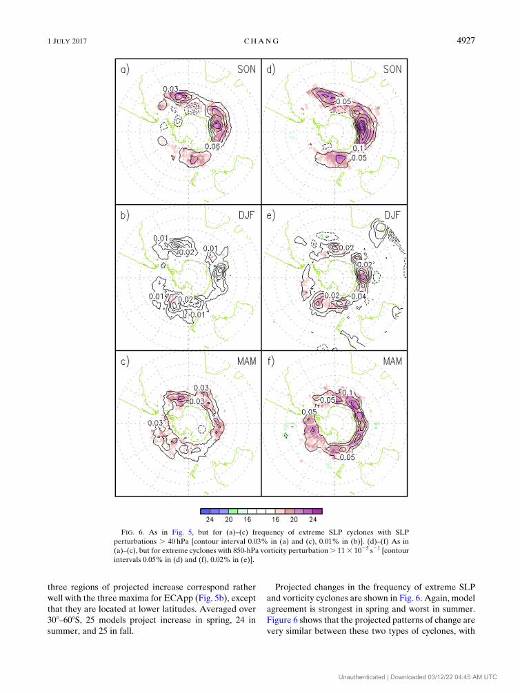
Projected changes in the frequency of extreme SLP

and vorticity cyclones are shown in Fig. 6. Again, model

agreement is strongest in spring and worst in summer.

Figure 6 shows that the projected patterns of change are

very similar between these two types of cyclones, with

FIG. 6. As in Fig. 5, but for (a)–(c) frequency of extreme SLP cyclones with SLP

perturbations . 40 hPa [contour interval 0.03% in (a) and (c), 0.01% in (b)]. (d)–(f) As in

(a)–(c), but for extreme cyclones with 850-hPa vorticity perturbation. 113 1025 s21 [contour

intervals 0.05% in (d) and (f), 0.02% in (e)].

1 JULY 2017 CHANG 4927

Unauthenticated | Downloaded 03/12/22 04:45 AM UTC

slightly larger increases projected in the frequency of

extreme vorticity cyclones as a result of their higher

climatological frequency (see Table 1).

Projected change in the frequency of cyclones with

extreme winds is shown in Fig. 7. Comparing Figs. 7a–c

to Fig. 6, projected increases in the frequency of cy-

clones with extreme 850-hPa winds tend to occur

slightly equatorward of projected increases in cyclones

with extreme vorticity or extreme SLP, but the patterns

of increase are very similar. As for cyclones with

FIG. 7. As in Fig. 5, but for (a)–(c) frequency of cyclones with extreme 850-hPa winds

[.45m s21; contour interval 0.03% for (a) and (c), 0.01% in (b)]; and (d)–(f) frequency of

cyclones with extreme near-surface winds [equivalent to top-5 cyclone in a JJAmonth; contour

interval 0.03% for (d) and (f), 0.01% in (e)].

4928 JOURNAL OF CL IMATE VOLUME 30

Unauthenticated | Downloaded 03/12/22 04:45 AM UTC

extreme surface wind, the projected increase in spring

(Fig. 7d) appears to be most robust, with those in

summer (Fig. 7e) and fall (Fig. 7f) projected to be more

noisy and limited in extent. Nevertheless, when aver-

aged over 308–608S, 17 of 19 models project increase in

summer, 15 in fall, and 16 in spring, showing overall

model agreement in projected overall increase over the

midlatitude SH.

5. Discussion

a. Sensitivity to definition of extreme cyclones

In the discussions above in sections 3 and 4, we largely

showed results for extreme cyclones based on the same

threshold, but for surface winds. Here, we briefly ex-

plore whether projected changes are sensitive to the

exact definition of extreme cyclones.

First, we examine extreme cyclones based on 850-hPa

vorticity. Projected percentage change based on the

same threshold of 1.1 3 1024 s21 for each model has

been shown in Fig. 3f. An alternative definition is based

on a vorticity threshold corresponding to an average of 5

cyclones per winter month. The threshold for each

model is listed in Table S3. The threshold ranges from

0.96 to 1.273 1024 s21. Projected percentage change for

each model is shown in Fig. 8a. Of the 27 models, 26

project an increase. While there are some quantitative

differences between the projections based on these two

definitions, model-to-model correlation of the projected

percentage change is 0.80. A third definition is based

on a vorticity threshold corresponding to an average of 1

cyclone per winter month (Table S3). The results for this

more extreme definition are shown in Fig. 8d. Again, 26 of

the 27models project an increase, and themodel-to-model

correlation between projections based on this definition

and the constant threshold is 0.88, while the correlation

with results based on the top-5 threshold is 0.86.

Similar results are found for extreme cyclones based

on maximum 850-hPa wind near the cyclone center

corresponding to the top-5 and top-1 cyclones per winter

month (Table S4; Figs. 8b and 8e), as well as maximum

near-surface wind near the cyclone center corre-

sponding to the top-5 and top-1 cyclones (Table S4;

Figs. 8c and 8f). For all cases, projected percentage

increase is highest for extreme cyclones defined by the

top-1 category (Tables S5 and S6 in the supplemental

material). The spatial patterns for the climatology and

projected changes for top-5 cyclones based on SLP,

850-hPa vorticity, and 850-hPa winds are shown in Fig.

S5 of the supplemental material. These results show

that our conclusion that CMIP5 models project a

significant increase in the number of extreme cyclones

over SH is not sensitive to the definition of extreme

cyclones.

b. Consistency between different kinds of extremecyclones

In the previous sections, we have examined CMIP5

projected changes of SH extreme cyclone activity based

on different definitions of cyclones and found overall

agreement in that nearly all models project an increase

in extreme cyclones regardless of the definition and that

the spatial distributions of the multimodel mean pro-

jected increase are all rather similar. Here, we would

like to further quantify the consistency between the

different definitions by examining the model-to-model

correlation between the projected changes (all averaged

over 308–608S) based on the different definitions.

Correlations for SH winter, for 5 of the 6 quantities

discussed in section 3, are shown in the top four rows of

Table 2. Highest consistency (with a correlation of 0.79)

is found between the projected percentage changes in

ECApp and the frequency of extreme cyclones defined

based on SLP perturbation using a threshold equivalent

to the top-5 cyclones in an average winter month during

the historical period. That is, when a model projects a

large (small) percentage change in ECApp, it is very

likely that it also projects a large (small) percentage

change in the frequency of extreme SLP cyclones.

Figure 9a shows a scatterplot between model-projected

changes in these two quantities for all four seasons

(separated by different colored symbols), showing pos-

itive correlation in all four seasons. However, results of

the four seasons do not seem to lie on the same re-

gression line, with the same percentage increase in

ECApp associated with larger increase in the frequency

of extreme SLP cyclones during summer. Note that most

points lie above the one-to-one line. This is likely be-

cause ECApp variability is dominated by moderate

rather than extreme cyclones. Since these extreme

events are rarest in summer, it is not surprising that the

relative change of extreme cyclones in summer with

respect to ECApp should be largest. Averaged over the

four seasons, the correlation of 0.61 (see Table 3) be-

tween projected changes based on these two quantities is

still relatively high.

Projected changes in the frequency of extreme cy-

clones defined based on SLP and 850-hPa vorticity

minima are also highly consistent, with a correlation of

0.70 for the SH winter, and 0.63 when averaged over the

four seasons. For these two quantities, results from all

four seasons seem to lie more or less on the one-to-one

line (Fig. 8c). Similarly, projected changes in the fre-

quency of extreme SLP cyclones and cyclones with ex-

treme 850-hPa winds are also highly consistent, with

1 JULY 2017 CHANG 4929

Unauthenticated | Downloaded 03/12/22 04:45 AM UTC

correlation of 0.69 for JJA, and 0.58 when averaged over

the four seasons. Figure 8b shows that again results for

all four seasons seem to lie on the same regression line.

Overall, correlations are rather high for winter and

lower for the other seasons, especially for summer. This

may be because these extreme cyclones are most frequent

in winter and least so in summer; hence, the statistics are

noisier in summer, giving rise to poorer agreement.

c. Consistency with mean flow change

Figure 2 highlights significant model-to-model differ-

ences in the magnitude of projected changes in extreme

cyclone statistics. Can we understand these differences?

O’Gorman (2010) showed that projected changes in

hemispheric averaged EKE found in CMIP3 model

simulations are proportional to projected changes

in MAPE. Hence, changes in MAPE are computed

for each pair of historical and future model simula-

tions. Here, the expression of MAPE formulated by

Orlanski and Katzfey (1991), integrated over 308–608Sand from 850 to 300 hPa, is used. MAPE is based en-

tirely on the temperature distribution, increasing

with larger temperature gradient and weaker static

stability. Apart from MAPE, we have also examined

FIG. 8. Projected percentage changes in the number of extreme cyclones in JJA, defined based on a threshold

equivalent to a top-5 cyclone permonth in JJA for eachmodel for: (a) 850-hPa vorticity perturbations, (b) 850-hPawinds,

and (c) near-surface winds. (d)–(f) As in (a)–(c), but for a threshold equivalent to a top-1 cyclone per month in JJA.

4930 JOURNAL OF CL IMATE VOLUME 30

Unauthenticated | Downloaded 03/12/22 04:45 AM UTC

changes in the zonal mean zonal wind at the 850-hPa level

to represent an alternative measure of mean flow change.

Note that the change in zonal mean zonal wind is largely

barotropic between 925 and 500hPa [not shown, but see

previous studies, such as Yin (2005)], suggesting that this

change represents change in the eddy-driven jet and is

largely a response to changes in eddy momentum flux

convergence. Changes in 850-hPa zonal wind are aver-

aged over 408–608S where the change is largest.

Correlations between model-projected changes in

MAPE and 850-hPa zonal wind with cyclone statistics

are shown in the last two rows of Table 2 for SH winter

and the last two rows of Table 3 for averages over all

four seasons. Consistent with O’Gorman (2010),

changes in MAPE are relatively well correlated with

changes in ECApp, which is an eddy variance statistics

similar to EKE. Figure 9d shows a scatterplot between

projected changes in MAPE and ECApp, showing

rather tight relationships for all four seasons. The

correlation between changes inMAPE and the number

of extreme SLP cyclones is also moderately high in

winter but is low in the other seasons. Results pre-

sented in Tables 2 and 3 show that changes in MAPE

(as well as 850-hPa zonal wind) are not well correlated

to changes in the number of extreme cyclones defined

based on 850-hPa vorticity, 850-hPa maximum wind, or

near-surface maximum wind. Thus, while projected

change inMAPE can, to a certain extent, ‘‘explain’’ the

projected change in variance statistics, it has little

utility in explaining change in the frequency of extreme

cyclones, especially extreme cyclones defined in terms

of maximum winds.

Tables 2 and 3 also show that projected changes in

850-hPa zonal wind are highly correlated with projected

changes in ECApp. This is likely due to the aforemen-

tioned fact that changes in 850-hPa zonal wind likely

represents a response to changes in eddy momentum

fluxes, which should be highly correlated with changes in

ECApp. Note that projected changes in 850-hPa zonal

wind are also not well correlated with changes in the

number of extreme cyclones. These results suggest that,

while changes in the frequency of extreme cyclones are

moderately correlated with changes in ECApp, they are

not significantly correlated with changes in MAPE

(Table 3). Thus, finding a mean flow metric that can

quantitatively explain the changes in the statistics of

extreme cyclones remains a challenge.

d. Sensitivity to model resolution

In the past, many studies have found that climate

model simulation of storm-track activity is highly de-

pendent on model resolution, with low-resolution

models simulating storm-track amplitudes that are

systematically too low (e.g., Boville 1991). Chang et al.

(2013) found that there is a moderate negative corre-

lation between model grid spacing and storm-track

amplitudes in 17 CMIP3 models. Here, we briefly ex-

amine whether CMIP5 projections show any strong

dependence on model resolution.

The horizontal resolution of each model simulation is

tabulated in Table S2. We have correlated the model

gridbox size (equal to the product of the latitude and

longitude grid spacing) with the climatology and pro-

jected changes in all the quantities we have discussed,

including both Eulerian and Lagrangian cyclone statis-

tics, and have not found any correlation that is signifi-

cant even at the 10% level. The climatology and

projected changes of extreme cyclones based on SLP,

vorticity, and 850-hPa winds, for 10 high-resolution and

10 low-resolution models, are shown in Figs. S6 and S7

of the supplemental material, respectively. We can see

that the projected changes from these two sets of models

are very similar. Thus, we conclude that projected

storm-track changes in CMIP5 simulations are not very

sensitive to model resolution. This is consistent with the

results of Bengtsson et al. (2009).

6. Summary and conclusions

In this study, projected changes in extreme cyclones in

the SH based on 26 CMIP5models have been computed.

Multiple definitions of extreme cyclones have been

examined, including intensity exceeding constant thresh-

olds of SLP perturbations, 850-hPa vorticity, and 850-hPa

TABLE 2. Model-to-model correlation between projected JJA percentage changes in the following: number of extreme cyclones based

on top 5 per JJA month (i) in terms of SLP perturbation, (ii) in terms of vorticity perturbation, (iii) in terms of 850-hPa maximum wind,

and (iv) in terms of near-surface maximum wind; (v) ECApp; (vi) MAPE; and (vii) zonal wind at 850 hPa (um850).

JJA SLP top 5 Vorticity top 5 850-hPa wind top 5 Surface wind top 5 ECApp MAPE

Vorticity top 5 0.70

850-hPa wind top 5 0.69 0.60

Surface wind top 5 0.62 0.52 0.56

ECApp 0.79 0.31 0.55 0.50

MAPE 0.58 0.28 0.09 0.16 0.73

um850 0.62 0.07 0.32 0.24 0.86 0.72

1 JULY 2017 CHANG 4931

Unauthenticated | Downloaded 03/12/22 04:45 AM UTC

winds, as well as variable thresholds corresponding to a

top-5 or top-1 cyclone in these three parameters and the

near-surface winds for each model. Results presented in

this study show that, under the RCP8.5 pathway, CMIP5

models project a significant increase in the frequency of

extreme cyclones between 1980–99 and 2081–2100 in all

four seasons regardless of the definition, with over 88% of

the models projecting an increase. The projected spatial

change patterns are also consistent between the differ-

ent definitions of extreme cyclones, with the largest in-

crease projected between 458 and 608S, extending from

the South Atlantic across the south Indian Ocean into the

South Pacific, with the maximum located over the south

Indian Ocean.

Overall, our results are consistent with those of Chang

et al. (2012), who showed that CMIP5 models project

FIG. 9. Scatterplots between CMIP5 model-projected percentage changes in (a) ECApp and number of extreme

SLP cyclones; (b) number of extreme SLP cyclones and number of extreme cyclones in terms of 850-hPa winds;

(c) number of extreme SLP cyclones and extreme cyclones in terms of 850-hPa vorticity; and (d) ECApp and

MAPE. All quantities are computed in the 308–608S band.

TABLE 3. As in Table 2, but the correlations have been averaged over all four seasons.

Averaged over all four seasons SLP top 5 Vorticity top 5 850-hPa wind top 5 Surface wind top 5 ECApp MAPE

Vorticity top 5 0.63

850-hPa wind top 5 0.58 0.51

Surface wind top 5 0.35 0.32 0.51

ECApp 0.61 0.40 0.53 0.20

MAPE 0.31 0.27 0.03 0.01 0.55

um850 0.41 0.02 0.32 0.01 0.68 0.49

4932 JOURNAL OF CL IMATE VOLUME 30

Unauthenticated | Downloaded 03/12/22 04:45 AM UTC

significant increase in the frequency of strong cyclones

defined in terms of SLP perturbations. Our results are

moderately consistent with those of Grieger et al. (2014),

who showed that an increase in the number of strong cy-

clones (top 5 percentile in terms of Laplacian in SLP)

is found in most of the model simulations they exam-

ined, but they found much more modest changes of

between 212.8% and 23.7%, with an ensemble mean

(from 9 simulations) of only 17.5%. Here, our results

show that, for similarly extreme cyclones, CMIP5

models project much larger changes. The difference is

likely due to the difference in scenarios used (their

simulations used the SRES A1B scenario, while here

we examined the higher-emission RCP8.5 simulations)

as well as different models included in the ensembles.

As discussed above, Bengtsson et al. (2009) found no

significant increase in extreme winds (at 925hPa) and

850-hPa vorticity near cyclones anywhere. However,

Bengtsson et al. (2009) only examined simulations based

on one model (ECHAM5). Our results indicate that, out

of the 26 CMIP5 models, a few project little changes or

even a decrease in the number of extreme cyclones; thus,

it is likely that the model used by Bengtsson et al. (2009)

has similar behavior to one of these models that project

small changes. Given the large spread found in the dif-

ferent model simulations, it is clear that general conclu-

sions cannot be drawn based on simulations using only

one (or even a few)model. It is of interest to note that the

twoMPI models (numbers 23 and 24), which use a newer

version of the ECHAMmodel (ECHAM6), both project

significant increase in ECApp, the frequency of extreme

850-hPawinds, as well as the number of extreme cyclones

(see Fig. 2). Finally, it was stated in the IPCC AR5

(Christensen et al. 2013, p. 1252) that ‘‘the CMIP5 model

projections show little evidence of change in the intensity

of winds associated with ETCs.’’ Our results show that

CMIP5 models clearly project significant increase in the

frequency of cyclones with extreme wind in the SH. It

should be noted that there are indications that the num-

ber of intense cyclones over the SHhas increased over the

past decades (Wang et al. 2016). However, trends derived

from different reanalysis datasets are quite different, and

it is not clear how the large changes in the quantity and

quality of observations may have impacted these trends.

Our results indicate that, while model-projected

changes in the frequency of extreme cyclones correlate

moderately well with changes in Eulerian indices such as

ECApp, which correlate significantly with changes in

MAPE, projected changes in the frequency of extreme

cyclones are not significantly correlated with those in

MAPE. Thus, there is still a challenge in finding mean

flowmetrics that can quantitatively explain the changes in

extreme cyclone frequency. In addition, our results

indicate that CMIP5 model simulations show no in-

dications that projected changes in extreme cyclone sta-

tistics are sensitive to model grid spacing. Nevertheless,

the highest-resolution model included in our ensemble

may still be unable to well resolve the impact of diabatic

heating on cyclone development (Willison et al. 2013),

and thus further examinations of climate simulations with

grid spacing of 25km or less are needed to resolve the

issue of whether diabatic impacts on cyclone development

may undergo significant changes in a warmer and moister

climate.

In this study, projections based on the high-emission

RCP8.5 pathway have been examined. For lower emis-

sion scenarios, Chang et al. (2012) showed that CMIP5-

projected change in variance statistics is roughly

proportional to the projected temperature change, but it

is not clear whether this result also applies to extreme

events. It would be of interest to examine projections

of lower-emission scenarios, especially since under these

scenarios the effects of ozone recovery may largely

cancel those of increasing greenhouse gas forcing during

SH summer (Polvani et al. 2011).

Acknowledgments. The author would like to thank

Kevin Hodges for providing the cyclone tracking code,

Albert Yau for assistance in downloading some of the

data, and the Earth System Grid and the climate mod-

eling centers for providing the CMIP5 data. The author

would also like to thank three anonymous reviewers for

providing comments that help to clarify the manuscript.

This research is supported by NSF Grant AGS-1261311

and NASA Grant NNX16AG32G.

REFERENCES

Alexander, L. V., S. F. B. Tett, and T. Jonsson, 2005: Recent ob-

served changes in severe storms over theUnited Kingdom and

Iceland. Geophys. Res. Lett., 32, L13704, doi:10.1029/

2005GL022371.

Ashley, W. S., and A. W. Black, 2008: Fatalities associated with

nonconvective high-wind events in the United States. J. Appl.

Meteor. Climatol., 47, 717–725, doi:10.1175/2007JAMC1689.1.

Barnes, E. A., N. W. Barnes, and L. M. Polvani, 2014: Delayed

Southern Hemisphere climate change induced by strato-

spheric ozone recovery, as projected by the CMIP5 models.

J. Climate, 27, 852–867, doi:10.1175/JCLI-D-13-00246.1.

Bengtsson, L., K. I. Hodges, and N. Keenlyside, 2009: Will extra-

tropical storms intensify in a warmer climate? J. Climate, 22,

2276–2301, doi:10.1175/2008JCLI2678.1.

Blackmon, M. L., 1976: A climatological spectral study of the

500mbgeopotential height of theNorthernHemisphere. J.Atmos.

Sci., 33, 1607–1623, doi:10.1175/1520-0469(1976)033,1607:

ACSSOT.2.0.CO;2.

Boville, B.A., 1991: Sensitivity of simulated climate tomodel resolution.

J. Climate, 4, 469–485, doi:10.1175/1520-0442(1991)004,0469:

SOSCTM.2.0.CO;2.

1 JULY 2017 CHANG 4933

Unauthenticated | Downloaded 03/12/22 04:45 AM UTC

Catto, J. L., E. Madonna, H. Joos, I. Rudeva, and I. Simmonds,

2015: Global relationship between fronts and warm conveyor

belts and the impact on extreme precipitation. J. Climate, 28,

8411–8429, doi:10.1175/JCLI-D-15-0171.1.

Chang, E. K. M., 2014: Impacts of background field removal on

CMIP5 projected changes in Pacific winter cyclone activity.

J. Geophys. Res. Atmos., 119, 4626–4639, doi:10.1002/

2013JD020746.

——, and Y. Fu, 2002: Interdecadal variations in Northern Hemi-

sphere winter storm track intensity. J. Climate, 15, 642–658,

doi:10.1175/1520-0442(2002)015,0642:IVINHW.2.0.CO;2.

——, Y. Guo, and X. Xia, 2012: CMIP5 multimodel ensemble

projection of storm track change under global warming.

J. Geophys. Res., 117, D23118, doi:10.1029/2012JD018578.

——,——,——, andM. Zheng, 2013: Storm-track activity in IPCC

AR4/CMIP3 model simulations. J. Climate, 26, 246–260,

doi:10.1175/JCLI-D-11-00707.1.

——, C. Zheng, P. Lanigan, A. M. W. Yau, and J. D. Neelin, 2015:

Significant modulation of variability and projected change in

California winter precipitation by extratropical cyclone ac-

tivity. Geophys. Res. Lett., 42, 5983–5991, doi:10.1002/

2015GL064424.

Christensen, J., and Coauthors, 2013: Climate phenomena and

their relevance for future regional climate change. Climate

Change 2013: The Physical Science Basis, T. F. Stocker et al.,

Eds., Cambridge University Press, 1217–1308, doi:10.1017/

CBO9781107415324.028.

Colle, B. A., F. Buonaiuto, M. J. Bowman, R. E. Wilson, R. Flood,

R. Hunter, A. Mintz, and D. Hill, 2008: New York City’s

vulnerability to coastal flooding. Bull. Amer. Meteor. Soc., 89,

829–841, doi:10.1175/2007BAMS2401.1.

——, Z. Zhang, K. A. Lombardo, E. K. M. Chang, P. Liu, and

M. Zhang, 2013: Historical evaluation and future prediction of

eastern North American and western Atlantic extratropical

cyclones in the CMIP5 models during the cool season.

J. Climate, 26, 6882–6903, doi:10.1175/JCLI-D-12-00498.1.

Collins, M., and Coauthors, 2013: Long-term climate change:

Projections, commitments and irreversibility. Climate Change

2013: The Physical Science Basis, T. F. Stocker et al., Eds.,

Cambridge University Press, 1029–1136, doi:10.1017/

CBO9781107415324.024.

Dee, D. P., and Coauthors, 2011: The ERA-Interim reanalysis:

Configuration and performance of the data assimilation

system. Quart. J. Roy. Meteor. Soc., 137, 553–597,

doi:10.1002/qj.828.

Feser, F., M. Barcikowska, O. Krueger, F. Schenk, R. Weisse, and

L. Xia, 2015: Storminess over the North Atlantic and north-

western Europe—A review. Quart. J. Roy. Meteor. Soc., 141,

350–382, doi:10.1002/qj.2364.

Grieger, J., G. C. Leckebusch, M. G. Donat, M. Schuster,

and U. Ulbrich, 2014: Southern Hemisphere winter cyclone

activity under recent and future climate conditions in

multi-model AOGCM simulations. Int. J. Climatol., 34, 3400–

3416, doi:10.1002/joc.3917.

Hodges, K. I., 1999: Adaptive constraints for feature tracking. Mon.

Wea.Rev., 127, 1362–1373, doi:10.1175/1520-0493(1999)127,1362:

ACFFT.2.0.CO;2.

Hoskins, B. J., and K. I. Hodges, 2002: New perspectives on the

Northern Hemisphere winter storm tracks. J. Atmos. Sci.,

59, 1041–1061, doi:10.1175/1520-0469(2002)059,1041:

NPOTNH.2.0.CO;2.

——, and ——, 2005: A new perspective on Southern Hemisphere

storm tracks. J. Climate, 18, 4108–4129, doi:10.1175/JCLI3570.1.

Lambert, S. J., and J. C. Fyfe, 2006: Changes in winter cyclone

frequencies and strengths simulated in enhanced greenhouse

warming experiments: Results from the models participating

in the IPCC diagnostic exercise. Climate Dyn., 26, 713–728,

doi:10.1007/s00382-006-0110-3.

Lim, E.-P., and I. Simmonds, 2002: Explosive cyclone development in

the Southern Hemisphere and a comparison with Northern

Hemisphere events.Mon.Wea.Rev., 130, 2188–2209, doi:10.1175/

1520-0493(2002)130,2188:ECDITS.2.0.CO;2.

——, and——, 2009: Effects of tropospheric temperature change on

the zonal mean circulation and SH winter extratropical cy-

clones. Climate Dyn., 33, 19–32, doi:10.1007/s00382-008-0444-0.

Lorenz, E. N., 1955: Available potential energy and themaintenance

of the general circulation. Tellus, 7A, 157–167, doi:10.1111/

j.2153-3490.1955.tb01148.x.

Neu, U., and Coauthors, 2013: IMILAST: A community effort to

intercompare extratropical cyclone detection and tracking

algorithms.Bull. Amer.Meteor. Soc., 94, 529–547, doi:10.1175/

BAMS-D-11-00154.1.

O’Gorman, P. A., 2010: Understanding the varied response of the

extratropical storm tracks to climate change.Proc. Natl. Acad.

Sci. USA, 107, 19 176–19 180, doi:10.1073/pnas.1011547107.

Orlanski, I., 2013: What controls recent changes in the circulation

of the SouthernHemisphere: Polar stratospheric or equatorial

surface temperatures? Atmos. Climate Sci., 3, 497–509.

——, and J. Katzfey, 1991: The life cycle of a cyclone wave in the

Southern Hemisphere. Part I: Eddy energy budget. J. Atmos.

Sci., 48, 1972–1998, doi:10.1175/1520-0469(1991)048,1972:

TLCOAC.2.0.CO;2.

Parish, T. R., and J. J. Cassano, 2003: The role of katabatic winds on

theAntarctic surfacewind regime.Mon.Wea. Rev., 131, 317–333,

doi:10.1175/1520-0493(2003)131,0317:TROKWO.2.0.CO;2.

Peixoto, J. P., and A. H. Oort, 1992: Physics of Climate. American

Institute of Physics, 520 pp.

Penny, S., G. H. Roe, and D. S. Battisti, 2010: The source of the

midwinter suppression in storminess over the North Pacific.

J. Climate, 23, 634–648, doi:10.1175/2009JCLI2904.1.Pezza, A. B., I. Simmonds, and J. A. Renwick, 2007: Southern

Hemisphere cyclones and anticyclones: Recent trends and

links with decadal variability in the Pacific Ocean. Int.

J. Climatol., 27, 1403–1419, doi:10.1002/joc.1477.——, H. A. Rashid, and I. Simmonds, 2012: Climate links and re-

cent extremes in Antartic sea ice, high-latitude cyclones,

southern annular mode and ENSO. Climate Dyn., 38, 57–73,

doi:10.1007/s00382-011-1044-y.

Pfahl, S., and H. Wernli, 2012: Quantifying the relevance of cy-

clones for precipitation extremes. J. Climate, 25, 6770–6780,

doi:10.1175/JCLI-D-11-00705.1.

Polvani, L. M., M. Previdi, and C. Deser, 2011: Large cancellation,

due to ozone recovery, of future Southern Hemisphere at-

mospheric circulation trends.Geophys. Res. Lett., 38, L04707,

doi:10.1029/2011GL046712.

Raible, C. C., P. M. Della-Marta, C. Schwierz, H. Wernli, and

R. Blender, 2008: Northern Hemisphere extratropical cyclones:

A comparison of detection and tracking methods and different

reanalysis. Mon. Wea. Rev., 136, 880–897, doi:10.1175/

2007MWR2143.1.

Rudeva, I., and I. Simmonds, 2015: Variability and trends of global at-

mospheric frontal activity and links with large-scale modes of var-

iability. J. Climate, 28, 3311–3330, doi:10.1175/JCLI-D-14-00458.1.

Simmonds, I., and K. Keay, 2000: Variability of Southern Hemisphere

extratropical cyclone behavior, 1958–97. J. Climate, 13, 550–561,

doi:10.1175/1520-0442(2000)013,0550:VOSHEC.2.0.CO;2.

4934 JOURNAL OF CL IMATE VOLUME 30

Unauthenticated | Downloaded 03/12/22 04:45 AM UTC

——,——, andE.-P. Lim, 2003: Synoptic activity in the seas around

Antarctica. Mon. Wea. Rev., 131, 272–288, doi:10.1175/

1520-0493(2003)131,0272:SAITSA.2.0.CO;2.

Sinclair, M. R., 1995: A climatology of cyclogenesis for the

Southern Hemisphere. Mon. Wea. Rev., 123, 1601–1619,

doi:10.1175/1520-0493(1995)123,1601:ACOCFT.2.0.CO;2.

Taylor, K. E., R. J. Stouffer, andG.A.Meehl, 2012:An overview of

CMIP5 and the experiment design. Bull. Amer. Meteor. Soc.,

93, 485–498, doi:10.1175/BAMS-D-11-00094.1.

Thompson,D.W. J., and S. Solomon, 2002: Interpretation of recent

Southern Hemisphere climate change. Science, 296, 895–899,

doi:10.1126/science.1069270.

Ulbrich, U., G. Leckebusch, and J. Pinto, 2009: Extra-tropical cy-

clones in the present and future climate: A review. Theor.

Appl. Climatol., 96, 117–131, doi:10.1007/s00704-008-0083-8.——, and Coauthors, 2013: Are greenhouse gas signals of Northern

Hemisphere winter extra-tropical cyclone activity dependent

on the identification and tracking algorithm?Meteor. Z., 22,

61–68, doi:10.1127/0941-2948/2013/0420.

Wallace, J. M., G.-H. Lim, and M. L. Blackmon, 1988: Rela-

tionship between cyclone tracks, anticyclone tracks, and

baroclinic waveguides. J. Atmos. Sci., 45, 439–462, doi:10.1175/

1520-0469(1988)045,0439:RBCTAT.2.0.CO;2.

Wang, X. L., Y. Feng, R. Chan, and V. Isaac, 2016: Inter-

comparison of extra-tropical cyclone activity in nine re-

analysis datasets. Atmos. Res., 181, 133–153, doi:10.1016/

j.atmosres.2016.06.010.

Wei, L., and T. Qin, 2016: Characteristics of cyclone climatology

and variability in the Southern Ocean. Acta Oceanol. Sin., 35,59–67, doi:10.1007/s13131-016-0913-y.

Willison, J., W. A. Robinson, and G. M. Lackmann, 2013: The im-

portance of resolving mesoscale latent heating in the North

Atlantic storm track. J. Atmos. Sci., 70, 2234–2250, doi:10.1175/JAS-D-12-0226.1.

Yin, J. H., 2005: A consistent poleward shift of the storm tracks

in simulations of 21st century climate.Geophys. Res. Lett., 32,L18701, doi:10.1029/2005GL023684.

Zappa, G., L. C. Shaffrey, K. I. Hodges, P. G. Sansom, and D. B.

Stephenson, 2013: A multimodel assessment of future pro-

jections of North Atlantic and European extratropical cy-

clones in theCMIP5 climatemodels. J. Climate, 26, 5846–5862,

doi:10.1175/JCLI-D-12-00573.1.

1 JULY 2017 CHANG 4935

Unauthenticated | Downloaded 03/12/22 04:45 AM UTC