Embed Size (px)
Citation preview

PROJECT TITLE: Air Toxics in Allegheny County: Sources, Airborne
Concentrations, and Human Exposure AGREEMENT #: 36946 REPORT: Final Technical Report REPORTING PERIOD: January 2005 – August 2008 ISSUED: January 2009 SUBMITTED TO: Allegheny County Health Department
3333 Forbes Ave Pittsburgh, PA 15213
PREPARED BY: Carnegie Mellon University
5000 Forbes Ave Pittsburgh, PA 15213
PIs: Allen Robinson, Neil Donahue, Cliff Davidson, Peter Adams, Mitch Small (412) 268 – 3657; (412) 268 – 3348 (fax) e-mail: [email protected]

2
Acknowledgements
This project was supported by the Allegheny County Health Department through the Clean
Air Fund and by the United States Environmental Protection Agency (EPA) through the
Community Scale Air Toxics Monitoring Program. The statements and conclusions in this
report are those of the authors and not those of the funding agencies.
This work was the primary focus of two PhD students at Carnegie Mellon University.
Jennifer Logue developed the automated gas phase organic air toxics instrument and performed
most of the data analysis. Andrew Lambe deployed the TAG instrument and led the analysis of
diesel particulate matter concentrations.
This work would not have been possible without extensive help from several contributors.
First and foremost, Jason Maranche and Darrell Stern from the Allegheny County Health
Department’s Air Quality Program who provided us with the baseline data, meteorological data,
technical support and answers to all of our questions. Our sincerest thanks go to Susanne Hering
and Nathan Kreisberg, of Aerosol Dynamics, Inc. and David Worton and Allen Goldstein of the
University of California Berkeley for all of their work developing the Thermal Desorption GC-
MS (TAG) instrument and aiding us in deploying it in the field in Allegheny County. We would
also like to thank Ted Palma and Mike Jones at the EPA for providing us with the preliminary
2002 NATA results and for answering our questions about the NATA modeling process. Lastly
we would like to thank Mike McCarthy and Hilary Hafner from Sonoma Technologies, Inc. for
providing us with data on the national distribution of air toxics concentrations.

3
Executive Summary
In January 2002, Carnegie Mellon University in collaboration with the Allegheny County
Health Department embarked on a project to investigate air toxic concentrations, risks and
sources in Allegheny County. The project was motivated by the concerns of citizens living near
Neville Island, a heavily industrialized area in the City of Pittsburgh.
Concentrations of 36 volatile organic air toxics were measured at six sites specifically chosen
to represent different source/exposure regimes. Two of the sites were in residential areas
adjacent to Neville Island; two of the sites were in downtown Pittsburgh, which has substantial
mobile source emissions; and two of the sites were located to characterize regional air toxic
concentrations. The two downtown sites and the two residential sites adjacent to Neville Island
were specifically chosen to represent high exposure areas with substantial local emissions. At
four of the six sites, 24-hour-average concentrations were measured on a one-in-six-day schedule
for a two-year period to characterize long-term and seasonal exposures. At three of the sites,
state-of-the-art instrumentation was deployed for shorter periods of time to make hourly
measurements of air toxic concentrations for source apportionment analysis.
Study-average concentrations of 13 of the target organic air toxics were greater than the
national 75th percentile at one or more of the baseline sites, including benzene, toluene,
propionaldehyde, tetrachloroethene, ethyl benzene, methylene chloride, styrene, 1,4-
dichlorobenzene, trichloroethene, m/p- and o-xylenes, methyl isobutyl ketone, and
chloromethane. Concentrations of many of these air toxics were a factor of two or more greater
at the urban sites than in South Fayette (the regional background site), indicating the substantial
influence of emissions from local sources. Concentrations of only two air toxics were greater
than the national 75th percentile in South Fayette: benzene and propionaldehyde. Therefore,
these two toxics present a countywide problem.
High-time resolved measurements revealed that most air toxics are characterized by periods
of low, relatively stable concentrations with intermittent, relatively short periods of higher
concentrations. The frequency and magnitude of these events varied from site to site, as a
function of wind direction and with the time of day. The high-time resolved data revealed strong
correlations between concentrations of certain air toxics and wind direction, helping to link high

4
concentration events with emissions from specific source regions. For example, at all three
intensive sites, high concentrations of benzene and other air toxics were observed when the sites
were downwind from Neville Island and Clairton, two areas with large industrial facilities.
Cancer and non-cancer health risks were estimated using traditional and advanced risk
models and published toxicity data. Figure ES-1 indicates that the additive cancer risk of the 36
target organic air toxics varied by less than a factor of 1.5 between the four baseline sites. The
highest risks were estimated for the downtown site. The spatial variation in cancer risks was
surprisingly modest given that three of the four baseline sites were in locations with substantial
emissions from local sources. The spatial variation in risk was so modest because two of the
most important air toxics, formaldehyde and carbon tetrachloride, are regionally distributed.
Benzene also contributed significantly to the cancer risks at all sites. Concentrations of
chlorinated air toxics such as trichloroethene and 1,4-dichlorobenzene were greatly elevated
downtown. Only one of the target air toxics, acrolein, was estimated to pose a non-cancer health
risk.
To more comprehensively assess air toxics risks in Allegheny County, the project also
analyzed archived air quality data measured by earlier studies. This broader assessment
considered 65 different air toxics. Figure ES-2 compares the additive cancer risks for four
different classes of air toxics: the 36 target organic air toxics, metals, polycyclic organic matter
(POM) and diesel particulate matter (DPM). Of these four classes of air toxics, DPM presented
the greatest cancer risks at all sites. DPM risks are 3 to 11 times the additive cancer risk of the
next highest class of air toxics, with the highest risks downtown. Only limited data are currently
available on the DPM levels in the county. These data indicate that downtown is a DPM hotspot,
with levels that are a factor of three to four higher than in other areas in the county. However,
even outside of the downtown area, DPM levels are still high enough such that it still poses the
greatest cancer risk.
A major goal of this project was to compare air toxic concentrations and risks in Allegheny
County to other locations in the United States. Figure ES-1 compares the cancer risk estimates
for Allegheny County to estimates for 14 other U.S. cites. The additive cancer risk of the 36
target organic air toxics varied by about a factor of 16 across this set of cities. Risks at all of the
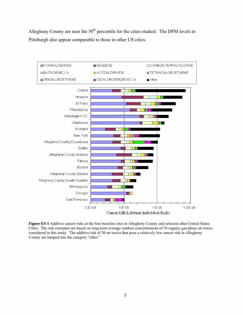
5
Allegheny County are near the 50th percentile for the cities studied. The DPM levels in
Pittsburgh also appear comparable to those in other US cities.
Figure ES-1 Additive cancer risks at the four baseline sites in Allegheny County and selected other United States Cities. The risk estimates are based on long-term average outdoor concentrations of 36 organic gas-phase air toxics considered in this study. The additive risk of 30 air toxics that pose a relatively low cancer risk in Allegheny County are lumped into the category “other.”

6
Figure ES-2 Additive cancer risk for different classes of air toxics. The estimates for the regional background are based on data from South Fayette and archived data from the Pittsburgh Supersite in Schenley Park (PAH, metals, and diesel PM).
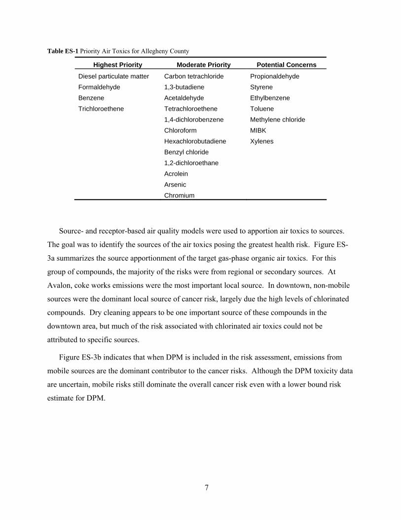
Based on the measured air toxic concentrations and risk estimates, a set of priority air toxics
for Allegheny County were identified. These priority toxics are listed in Table ES-1. Four air
toxics were designated as the highest priority: DPM, benzene, formaldehyde and trichloroethene.
All of these air toxics pose lifetime cancer risks greater than 10-5. Air toxics with a lifetime
cancer risk between 10-6 and 10-5 or estimated to pose non-cancer risks were classified as
moderate priority. The category “Potential Concerns” includes air toxics with higher than
average concentrations relative to national data but that are not estimated to pose health risks.
10-6
10-5
10-4
10-3
Ca
nce
r L
IR
RegionalDowntownAvalon
No
Met
als
Dat
a
No
PA
H D
ata
No
DP
M D
ata
No
PA
H D
ata
Die
sel P
M
Die
sel P
M
Vo
latil
e O
rga
nic
s
Vo
latil
e O
rga
nic
s
Vo
latil
e O
rgan
ics
Met
als
Me
talsPA
H
7
Table ES-1 Priority Air Toxics for Allegheny County
Highest Priority Moderate Priority Potential Concerns
Diesel particulate matter Carbon tetrachloride Propionaldehyde
Formaldehyde 1,3-butadiene Styrene
Benzene Acetaldehyde Ethylbenzene
Trichloroethene Tetrachloroethene Toluene
1,4-dichlorobenzene Methylene chloride
Chloroform MIBK
Hexachlorobutadiene Xylenes
Benzyl chloride
1,2-dichloroethane
Acrolein
Arsenic
Chromium
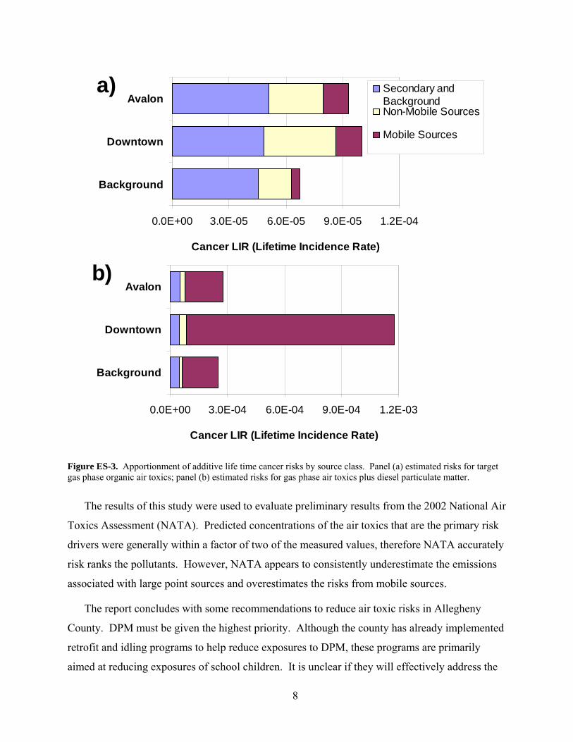
Source- and receptor-based air quality models were used to apportion air toxics to sources.
The goal was to identify the sources of the air toxics posing the greatest health risk. Figure ES-
3a summarizes the source apportionment of the target gas-phase organic air toxics. For this
group of compounds, the majority of the risks were from regional or secondary sources. At
Avalon, coke works emissions were the most important local source. In downtown, non-mobile
sources were the dominant local source of cancer risk, largely due the high levels of chlorinated
compounds. Dry cleaning appears to be one important source of these compounds in the
downtown area, but much of the risk associated with chlorinated air toxics could not be
attributed to specific sources.
Figure ES-3b indicates that when DPM is included in the risk assessment, emissions from
mobile sources are the dominant contributor to the cancer risks. Although the DPM toxicity data
are uncertain, mobile risks still dominate the overall cancer risk even with a lower bound risk
estimate for DPM.
8
0.0E+00 3.0E-05 6.0E-05 9.0E-05 1.2E-04
Background
Downtown
Avalon
Cancer LIR (Lifetime Incidence Rate)
Secondary andBackgroundNon-Mobile Sources
Mobile Sources
a)
0.0E+00 3.0E-04 6.0E-04 9.0E-04 1.2E-03
Background
Downtown
Avalon
Cancer LIR (Lifetime Incidence Rate)
b)
Figure ES-3. Apportionment of additive life time cancer risks by source class. Panel (a) estimated risks for target gas phase organic air toxics; panel (b) estimated risks for gas phase air toxics plus diesel particulate matter.
The results of this study were used to evaluate preliminary results from the 2002 National Air
Toxics Assessment (NATA). Predicted concentrations of the air toxics that are the primary risk
drivers were generally within a factor of two of the measured values, therefore NATA accurately
risk ranks the pollutants. However, NATA appears to consistently underestimate the emissions
associated with large point sources and overestimates the risks from mobile sources.
The report concludes with some recommendations to reduce air toxic risks in Allegheny
County. DPM must be given the highest priority. Although the county has already implemented
retrofit and idling programs to help reduce exposures to DPM, these programs are primarily
aimed at reducing exposures of school children. It is unclear if they will effectively address the

9
downtown DPM hotspot. To reduce DPM concentrations in the downtown area will likely
require new initiatives, including activity based and retrofit programs. More data are needed to
quantify the spatial extent of the downtown DPM hotspot. Benzene is another important air
toxic with substantial local emissions. Currently, a large effort is underway to reduce emissions
from the Clairton Coke Works, the largest point source of benzene in Allegheny County. This
should reduce benzene risks throughout the county, but there are also substantial benzene
emissions from sources on Neville Island. New programs are needed to more effectively control
those emissions.

10
Table of Contents
Acknowledgements................................................................................................................... 2
Executive Summary .................................................................................................................. 3
Table of Contents.................................................................................................................... 10
Table of Figures ...................................................................................................................... 14
Table of Tables ....................................................................................................................... 22
Chapter 1. Introduction ........................................................................................................... 23
1.1 Project Objectives ......................................................................................................... 24
1.2 Outline of the report...................................................................................................... 24
Chapter 2. Experimental Methods: Monitoring Sites and Instrumentation ............................ 26
2.1 Measurement Locations ................................................................................................ 26
2.2 Target Compounds........................................................................................................ 27
2.3 Baseline Measurements ................................................................................................ 30
2.3 Intensive Measurements................................................................................................ 30
2.3.1 Automated Gas Phase Measurements.................................................................... 30
2.3.1 Instrument Calibration ........................................................................................... 34
2.3.1 Instrument Evaluation............................................................................................ 34
2.4 Measurement of semivolatile and condensed phase air toxics ..................................... 36
2.5 Meteorology Measurements.......................................................................................... 38
Chapter 3. Spatial Variation in Air Toxic Concentrations and Health Risks ......................... 40
3.2 Methods......................................................................................................................... 40
3.2.1 Statistical Analysis of Baseline Data ..................................................................... 40
3.2.2 Risk Assessment Models ....................................................................................... 41

11
3.3 Air Toxic Concentrations in Allegheny County ........................................................... 46
3.3.1 Spatial Variation in Gas Phase Air Toxic Concentrations..................................... 48
3.3.2 Diesel Particulate Matter (DPM) ........................................................................... 54
3.4 Risk Analysis ................................................................................................................ 56
3.4.1 Cancer Risks of Gas Phase Organic Air Toxics .................................................... 56
3.4.2 Non-Cancer Risks of Gas Phase Organic Air Toxics ............................................ 59
3.4.3 Diesel Particulate Matter Health Risks .................................................................. 61
3.4.5 Comparing Health Risks of Different Classes of Air Toxics ................................ 62
3.4.6 Comparison of Risks in different U.S. Cities ........................................................ 65
3.4.7 Interactive Risk Model Analysis............................................................................ 67
3.5 Indentifying Priority Air Toxics ................................................................................... 71
Chapter 4. Temporal Variations in Air Toxics Concentrations .............................................. 72
4.1 Times Series of Priority Air Toxics .............................................................................. 72
4.2 The Effect of Wind Direction on Air Toxics Concentrations....................................... 75
4.3 Temporal Patterns in Air Toxics Concentrations.......................................................... 82
4.3.1 Day of the Week Patterns in Air Toxics Concentrations....................................... 83
4.3.2 Diurnal Patterns of Air Toxics Concentrations...................................................... 84
4.3.3 Seasonal Patterns of Air Toxics Concentrations.................................................... 87
4.4 Chlorinated Compounds ............................................................................................... 88
Chapter 5. Receptor Modeling of Air Toxic Concentrations and Risks ................................. 92
5.1 Cancer Risk from Baseline and Intensive Studies ........................................................ 92
5.2 Receptor Modeling........................................................................................................ 93
5.2.1 Positive Matrix Factorization (PMF) ..................................................................... 93
5.2.2 Pollutants Apportioned Using PMF....................................................................... 94

12
5.2 Avalon PMF solution.................................................................................................... 95
5.2.1 Discussion of Avalon PMF Results ..................................................................... 105
5.3 Downtown PMF solution............................................................................................ 107
5.3.1 Discussion of Downtown PMF Results ............................................................... 116
5.4 Carnegie Mellon University PMF Results.................................................................. 118
5.4.1 Discussion of the Carnegie Mellon University PMF Results .............................. 121
5.5 Conclusions................................................................................................................. 122
Chapter 6. Source Apportionment of Diesel Particulate Matter Using Highly Time-Resolved
Measurements of Organic Molecular Markers and Black Carbon ............................................. 124
6.1. Introduction................................................................................................................ 124
6.2 PMF Analysis ............................................................................................................. 124
6.3 CMB Analysis............................................................................................................. 128
Chapter 7. Risk Synthesis: Apportioning Risks to Sources in Allegheny County ............... 131
7.1 Apportioning Risks from Air Toxics not included in PMF ........................................ 131
7.1.1 Formaldehyde ...................................................................................................... 131
7.1.2 Carbon tetrachloride............................................................................................. 132
7.1.3 Acetaldehyde........................................................................................................ 133
7.1.4 1,3-butadiene........................................................................................................ 133
7.1.5 Hexachlorobutadiene, 1,2-Dichloropropane, and Vinyl Chloride ....................... 134
7.1.6 Acrolein................................................................................................................ 134
7.2 Apportionment of Risks to Sources ............................................................................ 135
7.3 Conclusions................................................................................................................. 139
Chapter 8. Evaluating NATA: Comparison of predicted and measured air toxic
concentrations, sources, and risks............................................................................................... 140
8.1 Target Air Toxics........................................................................................................ 141

13
8.2 Comparison of Predicted and Measured Outdoor Concentrations ............................. 142
8.3 Risk Ranking of Pollutants ......................................................................................... 146
8.4 Comparison of Source Apportionment Estimates....................................................... 151
8.5 Conclusions................................................................................................................. 154
Chapter 9. Synthesis, Conclusions and Recommendations .................................................. 155
9.1 Synthesis by Pollutant................................................................................................. 155
9.1.1 Diesel Particulate matter (DPM).......................................................................... 155
9.1.2 Formaldehyde ...................................................................................................... 156
9.1.3 Benzene................................................................................................................ 157
9.1.4 Chlorinated Compounds ...................................................................................... 157
9.1.5 Carbon Tetrachloride ........................................................................................... 159
9.1.6 1,3-Butadiene ....................................................................................................... 159
9.1.7 Acetaldehyde........................................................................................................ 159
9.1.8 Acrolein................................................................................................................ 159
9.1.9 Metals................................................................................................................... 160
9.2 Synthesis by Source .................................................................................................... 160
9.3 Spatial Variability ....................................................................................................... 161
9.4 Recommendations....................................................................................................... 161
References............................................................................................................................. 163

14
Table of Figures
Figure ES-1 Additive cancer risks at the four baseline sites in Allegheny County and selected other
United States Cities. The risk estimates are based on long-term average outdoor concentrations
of 36 organic gas-phase air toxics considered in this study. The additive risk of 30 air toxics that
pose a relatively low cancer risk in Allegheny County are lumped into the category “other.”...... 5
Figure ES-2 Additive cancer risk for different classes of air toxics. The estimates for the regional
background are based on data from South Fayette and archived data from the Pittsburgh
Supersite in Schenley Park (PAH, metals, and diesel PM)............................................................. 6
Figure ES-3. Apportionment of additive life time cancer risks by source class. Panel (a) estimated
risks for target gas phase organic air toxics; panel (b) estimated risks for gas phase air toxics plus
diesel particulate matter. ................................................................................................................. 8
Figure 2.1 Location of air toxics monitoring sites. ............................................................................ 27
Figure 2.2 Schematic of automated gas-phase organic air toxic instrument developed and deployed
by Carnegie Mellon University during intensive studies (Millet, 2005). ..................................... 31
Figure 2.3. Comparison of air toxic concentrations measured with automated GC-MS/FID system
and the SUMMA canisters at the Avalon Site. ............................................................................. 36
Figure 2.4 Schematic diagrams showing heated zones and flow paths during sampling/analysis
mode (left) and thermal desorption mode (right). (From Dr. Nathan Kreisberg, Aerosol
Dynamics Inc.).............................................................................................................................. 38
Figure 2.5 Location of Hammerfield site relative to Diamond Building and Carnegie Mellon
University intensive sites. ............................................................................................................. 39
Figure 3.1. (a) Study-average air toxic concentrations measured at the four baseline sites. (b) Ratio
of study average concentrations measured at the three urban baseline sites to those measured in
South Fayette. Ratios greater than one indicate that concentrations at the urban site are greater
than those in South Fayette. .......................................................................................................... 51
Figure 3.2. Same as in Figure 3.1but for more regional air toxics. (a) Study-average air toxic
concentrations measured at the four baseline sites. (b) Ratio of study average concentrations

15
measured at the three urban baseline sites to those measured in South Fayette. Ratios greater
than one indicate that concentrations at the urban site are greater than those in South Fayette. .. 52
Figure 3.3. Comparison of study-average concentrations measured at the four baseline sites to
national air toxic data. The national data are multi-year average concentrations measured at
about 150 urban and suburban sites throughout the United States; these data are presented using
a box and whisker plot. The boxes extend from the 25th percentile to the 75th percentile of the
national data with the center line representing the median concentration. The whiskers extend to
the 5th and 95th percentiles of the national data........................................................................... 53
Figure 3.4. Average BC or EC concentrations at monitoring sites in and around Allegheny County
and in other locations in the United States. Downtown measurements were made during the 2008
intensive at the Diamond Building; the data from the other Pittsburgh area sites were measured
in 2001 and 2002 during the Pittsburgh Air Quality Study; the data from the other locations are
averages of measurements collected as part of the EPA Speciation Trends Network (STN) during
June, July and August of 2001 through 2004. .............................................................................. 55
Figure 3.5. Cancer lifetime incidence rate, LIR, calculated using the study upper limit of the 95%
confidence interval of the study-average concentration. The vertical red dashed line indicates a
risk of 10-6 of (1 in a million)........................................................................................................ 58
Figure 3.6 Additive cancer lifetime incidence rate, LIR, posed by the 38 gas-phase organic air toxics
measured at the four baseline sites................................................................................................ 59
Figure 3.7 Additive cancer lifetime incidence rate, LIR, for different target posed by the 38 gas-
phase organic air toxics measured at the four baseline sites......................................................... 60
Figure 3.8 Hazard quotients (HQ) for non-cancer chronic health effects. The dashed vertical red
line indicates a HQ of one. Air toxics with a HQ less than one are thought not to pose a non-
cancer risk. .................................................................................................................................... 61
Figure 3.9 Comparison of additive cancer risk for different classes of air toxics. The estimates for
the regional background are based on data from the South Fayette site collected as part of this
study (volatile organics) and archived data from the Pittsburgh Supersite in Schenley Park (PAH,
metals, and diesel PM).................................................................................................................. 63

16
Figure 3.10 Comparison of hazard quotients for different classes of air toxics measured at regional
background sites. The dashed line represents a hazard quotient of 1 indicating potential for non-
cancer risks and a hazard quotient of .1, an indicator that concentrations being a factor of ten
less then their RfC value. .............................................................................................................. 64
Figure 3.11 Non-cancer hazard quotients of metals calculated using archived data (6). The Schenley
Park site is the urban background site........................................................................................... 64
Figure 3.12 Comparison of additive cancer risks at the four baseline sites in Allegheny County to
other cities in the United States. The comparisons are based on the 38 organic gas-phase air
toxics considered in this study. ..................................................................................................... 66
Figure 3.13. Comparison of additive lifetime incidence rate (LIR) due to metal exposures for
selected cities and six sites in the Pittsburgh area (indicated by * symbol). ................................ 67
Figure 3.14 Best and worst case scenarios for synergistic/antagonistic non-cancer health effects.
Symbols represent the additive hazard index; the error bars extend to the best and worse possible
values for the hazard index. .......................................................................................................... 69
Figure 3.15 Enhancement factors for each target system that has a potential for risk above threshold.
(HIint,p greater than 1, LIRint,p greater than 10-4). The maximum possible enhancement is 10, the
assumed value of Mjk in the interactive risk model. Format for listing interaction pairs is A/B
where A is the pollutant being affected by pollutant B. ............................................................... 70
Figure 4.1 Time series of hourly concentrations measured during October 2006 at the Avalon site.
The shaded regions indicate two of the many plumes that influenced this site. ........................... 73
Figure 4.2 Time series of hourly air toxic concentrations measured during March-April 2008 at the
downtown Diamond Building site. ............................................................................................... 74
Figure 4.3 Time series of hourly air toxic concentrations measured during June 2007 at Carnegie
Mellon University. ........................................................................................................................ 75
Figure 4.4 Wind roses for the two meteorological stations, Avalon and Hammerfield. ................... 76
Figure 4.5 Average air toxic concentrations (g/m3) as a function of wind direction for high time
resolved measurements downtown, at the urban background site, and at the Avalon site.
Averages calculated by binning data based on wind direction, as discussed in the text. ............. 78
17
Figure 4.6 Map of Allegheny County with the two industrial areas affecting air toxics
concentrations outlined. a) Neville Island area and b) up river industrial area ........................... 80
Figure 4.7 Map of the Neville Island area shown in section (a) from Figure 4.6.............................. 81
Figure 4.8 Map of the upriver industrial area shown as section (b) in Figure 4.6. ............................ 81
Figure 4.9 Average weekday and weekend concentrations of air toxics measured during the
intensive campaigns. The error bars indicate the 5th and 95th percentile confidence interval of the
mean using the bootstrap method. ................................................................................................ 84
Figure 4.10 Average diurnal profiles of air toxic concentrations at the three intensive sites. Symbols
indicate the mean concentration at each hour and error bars represent 95th percentile confidence
interval on the mean. Note that concentration scale changes between sites. ............................... 86
Figure 4.11 Average diurnal profiles of condensed phase compounds associated with motor vehicle
emissions measured at the Diamond Building. Symbols represent the mean concentration and
error bars represent the standard error of the mean. Note that concentration scale changes
between sites. ................................................................................................................................ 87
Figure 4.12 Seasonal patterns of selected air toxics measured during the baseline study. ................ 88
Figure 4.13 Quarterly average concentrations of trichloroethene measured at the Flag Plaza site
from 1997 to the second quarter of 2008. ..................................................................................... 89
Figure 4.15 1,4-dichlorobenzene concentrations as a function of wind direction. Also shown are the
location and distance to the two point sources that report 1,4-dichlorobenzene emissions in
Allegheny County. ........................................................................................................................ 90
Figure 4.16 On the left is the average concentration of methylene chloride as a function of wind
direction. On the right is the average concentration during the week and weekend. The error
bars indicate the 95th percentile confidence intervals of the mean. .............................................. 91
Figure 5.1 Comparison of calculated cancer risks from intensive and baseline studies. ................... 93
Figure 5.2 Factor contributions to air toxic concentrations at the Avalon site. ................................. 96
Figure 5.3 Apportionment of cancer risk for the Avalon site. ........................................................... 97
Figure 5.4 Mean contribution for Benzene factor as a function of wind direction............................ 98

18
Figure 5.5 Diurnal patterns of factor contribution and factor contribution as a function of day of the
week for the Benzene factor. ........................................................................................................ 98
Figure 5.6 Comparison of the Neville Island Benzene Factor to emission profiles for two coke
works in Allegheny County. Shenango is located on Neville Island near Avalon and Clairton is
the largest coke works in Allegheny County. ............................................................................... 99
Figure 5.7 Mean factor contribution of the downtown factor in Avalon as a function of wind
direction. ..................................................................................................................................... 100
Figure 5.8 Comparison of the downtown factor to mobile source profiles (33, 34)........................ 100
Figure 5.9 Comparison of Allegheny County Sanitary Authority emissions profile and the profile of
the ASCA PMF factor................................................................................................................. 101
Figure 5.10 Mean concentration of the ACSA as a function of wind direction. ............................. 102
Figure 5.12 Diurnal patterns of factor contribution and factor contribution as a function of day of the
week for the Styrene factor. ........................................................................................................ 103
Figure 5.13 Comparison of large styrene emitting point source profiles and the profile of the Styrene
Factor. ......................................................................................................................................... 104
Figure 5.14 Mean concentration of secondary/background factor as a function of wind direction. 105
Figure 5.15 Diurnal patterns of factor contribution and factor contribution as a function of day of the
week for the Secondary/Background Factor............................................................................... 105
Figure 5.16 Apportionment of risk associated with 36 target gas phase organic air toxics............. 107
Figure 5.17 Factor contributions to individual compound concentrations at the downtown site. ... 108
Figure 5.18 Risk apportionment at the Diamond Building site. ...................................................... 109
Figure 5.19 Average contribution of Pittsburgh Factor as a function of the day of the week or time
of the day..................................................................................................................................... 110
Figure 5.20 On the left is the mean concentration of the Pittsburgh factor as a function of wind
direction. On the right is the mean concentration of black carbon (g m-3), BC, as a function of
wind direction. ............................................................................................................................ 110

19
Figure 5.21 Comparison of the species distribution in the Downtown Factor to source profiles for
gasoline and diesel vehicles (33, 34). Comparison based on compounds reported in gasoline and
diesel profiles, 89% of the factor mass. ...................................................................................... 111
Figure 5.22 The mean contribution of the Southern Toluene/Benzene Factor as a function of wind
direction. ..................................................................................................................................... 112
Figure 5.23 Diurnal patterns of factor contribution and factor contribution as a function of day of the
week for the Southern Benzene/Toluene Factor. ........................................................................ 112
Figure 5.24 Comparison of the species distribution in Southern Toluene/Benzene Factor to source
profiles for large industrial in Clairton area and gasoline vehicle emissions. ............................ 113
Figure 5.25 Diurnal patterns of factor contribution and factor contribution as a function of day of the
week for the local industry factor. .............................................................................................. 114
Figure 5.26 Diurnal patterns of factor contribution and factor contribution as a function of day of the
week for the Secondary/Background Factor............................................................................... 115
Figure 5.27 Temporal patterns of the Alkybenzene Factor. ............................................................ 116
Figure 5.28 The contribution of the alkyl benzene factor as a function of wind direction at the
Diamond Building....................................................................................................................... 116
Figure 5.29 PMF apportionment of cancer risks at the Diamond Building..................................... 117
Figure 5.31 Factor contributions to individual compounds concentrations at the urban background
(CMU) site. ................................................................................................................................. 118
Figure 5.32 Risk apportionment at the Carnegie Mellon University site. ....................................... 119
Figure 5.33 Average contribution of the southeastern factor as a function of wind direction. The
direction of the three major air toxics emitters in the Clairton Area relative to the Carnegie
Mellon University site are indicated on the graph. ..................................................................... 120
Figure 5.34 Comparison of the Southeastern Factor and the dominant point sources from the up
river industrial areas for the pollutants reported emitted by the point sources. .......................... 120
Figure 5.35 Comparison of the local sources factor to motor vehicle source profiles. ................... 121
Figure 5.36 Sources of risks from for PMF apportionment of the CMU intensive risks................. 122

20
Figure 6.1: (a) PMF apportionment for compounds included as fitting species in a three-factor
model (FPEAK = -0.2). (b) Time series for BC apportioned to each source factor over a three-
week period. Vertical grey bars are overnight periods (12-6AM), and vertical cyan bars are
weekends..................................................................................................................................... 126
Figure 6.2: (a) Ratio-ratio plot for norhopane and hopane with BC used as the reference species. (b)
Ratio-ratio plot for trisnorhopane and hopane, with norhopane used as the reference species.
Ambient data are shown in black circles and source profiles are shown in colored markers.
Numbers indicate source profiles: (1) Fujita MDD (2) Fujita HW (3) Fujita HDD (4) Fujita HCS
(5) Schauer MDD (6) Fujita MDD-HDD (50%-50%) composite (7) Fujita SI-HC (8) Fujita SI-
HW (9) Fujita SI-BW (10) Fujita SI-BC (11) Schauer catalyst auto (12) Fujita SI-LW (13) Fujita
SI-LC (14) Fujita SI-LW-HC (99%-1%) composite (14) Fujita SI-LW-HC (97.5%-2.5%) (15)
Fujita SI-LW-HC (95%-5%) (16) Fujita SI-LW-HC (90%-10%) (D) PMF “Diesel” (G) PMF
“Gasoline” (I) PMF “Industrial”. Fujita source profiles are from (43, 44); Schauer source
profiles are from (33, 34). ........................................................................................................... 127
Figure 6.3: Comparison of PMF and CMB apportionment of black carbon (BC) to (a) diesel and (b)
gasoline vehicles. Results are shown CMB solutions with different composite gasoline profiles,
as discussed in the text................................................................................................................ 128
Figure 6.4: Histogram of DPM concentrations estimated using CMB at the downtown and urban
background (PAQS Supersite) sites. Study average DPM estimates at the downtown site ranged
from 3.0 – 4.3 g m-3 depending on the CMB scenario, compared to 0.8 – 1.1 g m-3 at the urban
background site for the same set of CMB scenarios. Also shown are “median” estimates of the
DPM cancer risks which are based on the best-estimate DPM potency factor. ......................... 130
Figure 7.1 Source apportionment of the additive cancer risk for the 36 target gas-phase organic air
toxics at the Avalon site. ............................................................................................................. 136
Figure 7.2 Source apportionment of the additive cancer risk for 36 target gas-phase organic air
toxics in downtown Pittsburgh.................................................................................................... 137
Figure 7.3 Source apportionment of the additive cancer risk for 36 target gas-phase organic air
toxics in South Fayette................................................................................................................ 138

21
Figure 7.4 Additive cancer for gas-phase organic air toxics and DPM for each of the sites divided
into regional/secondary contribution, mobile source contribution, and industrial contribution. 139
Figure 8.1 Comparison of measured and predicted annual average concentrations of gas-phase
organic air toxics......................................................................................................................... 144
Figure 8.2 Comparison of measured and predicted annual average concentrations of selected
gasphase organic air toxics. ........................................................................................................ 145
Figure 8.3 Measured versus modeled concentrations for metals measured at Avalon and Schenley
Park sites. .................................................................................................................................... 146
Figure 8.4 Comparison of additive cancer risk for preliminary 2002 NATA to estimates based on
measured concentrations. The category “other” includes: chloroform, 1,2-dichloroethane,
hexachlorobutadiene, benzyl chloride, methylene chloride, 1,2-dicloropropane, 1,1,2,2-
tetrachloroethane, 1,1-dichloroethane, 1,1,2-trichloroethane, vinyl chloride, and bromoform.. 149
Figure 8.5 Comparison of additive cancer risk for preliminary 2002 NATA to estimates based on
measured concentrations for metals............................................................................................ 150
Figure 8.6 Comparison of NATA and receptor model source apportion for benzene..................... 152
Figure 8.7 Comparison of NATA and receptor model apportionment of formaldehyde. ............... 153
Figure 9.1 A comparison of air toxic cancer risks with other common risks. ................................. 156

22
Table of Tables
Table ES-1 Priority Air Toxics for Allegheny County .................................................................. 7
Table 2.1 Summary of measurements taken during project......................................................... 27
Table 2.2 Air toxics considered in this study and the locations and timeframes of their
measurement. .......................................................................................................................... 29
Table 3.1 Toxicity data for risk analysis. ..................................................................................... 43
Table 3.2 Summary of baseline air toxic concentrations in pptv ................................................. 47
Table 3.2 (continued) Summary of baseline air toxic concentrations in pptv.............................. 48
Table 3.3 Priority Air Toxics for Allegheny County ................................................................... 71
Table 5.1 Pollutants included in PMF analysis ............................................................................ 95
Table 8.1 Pollutants included in the NATA evaluation. ........................................................... 142
Table 8.2 Risk ranking of air toxics from highest cancer risks to lowest for the 10 risk drivers
from NATA and the health risks analysis presented in Chapter 3........................................ 151

23
Chapter 1. Introduction
This is the final technical progress report of the project “Air Toxics in Allegheny County:
Sources, Airborne Concentrations, and Human Exposure,” supported by the Allegheny County
Health Department under Agreement #36946. This project was motivated by concerns of
citizens about exposures to air pollutants emitted by large industrial facilities and other sources.
Although Pittsburgh’s steel days are over, there are still 186 point sources in the county, 87 of
which are large enough to be required to report air toxic emissions (1). In addition, much of this
industrial activity is clustered in certain areas, potentially creating concerns with environmental
inequality (2).
This project specifically investigated the exposures, health risks, and sources of hazardous air
pollutants or air toxics. Air toxics are pollutants that are known or suspected to cause serious
health effects. Some of these species also play an important role in secondary aerosol and ground
level ozone formation (3). The Environmental Protection Agency (EPA) currently classifies 187
pollutants as air toxics. The list includes a diverse set of compounds including organics,
chlorinated compounds, and metals.
In the 1990s EPA initiated the National Air Toxics Assessment (NATA) to determine the air
toxics that pose the greatest risk to human health. The 1996 NATA estimated nationwide
exposures to 33 air toxics which were thought to pose the greatest health risks. In 1999, the
assessment was expanded to include 177 compounds. NATA determined that benzene presented
the greatest potential cancer risk predominately from on-road emissions, but that the total cancer
risk associated with air toxics (1 to 25 in a million) was significantly smaller than the lifetime
cancer rate in the US (1 in 3) (4). The greatest non-cancer risk was found to be respiratory
issues. However large uncertainties still exist regarding sources, exposure and health risks,
mostly due to a lack of actual concentration measurements. Data are needed to evaluate
predicted concentrations and to determine actual exposure.
This project investigated 65 different air toxics that were specifically chosen because they
were identified as priority pollutants by NATA and/or there are known substantial emissions in
Allegheny County. Atmospheric concentrations of as many as 52 air toxics were measured at
different sites throughout the county. To provide a more comprehensive assessment, the project

24
also utilized archived data for 13 additional air toxics. Concentrations at different sites were
compared to assess the spatial variation in exposure. Traditional and advanced models were
used to assess the air toxic health risk. Source- and receptor-based models were used to
apportion air toxics concentrations and health risks to sources. Finally, air toxic concentrations
and risks in Allegheny County were compared to other data from other United States cities.
1.1 Project Objectives
The overall project had five primary objectives:
1. Measure airborne concentrations of a large number of gas and particulate air toxics
around Neville Island, in downtown Pittsburgh, and at a background site;
2. Estimate human exposure and health risks in the vicinity of sources and at the
background location;
3. Quantify the contribution of different sources (regional background, industrial,
mobile) to airborne concentrations and estimated health risks;
4. Establish the relative importance of regional transport versus local sources to air
toxics exposures in the County; and
5. Compare air toxic concentrations and estimated health risks in Allegheny County to
other areas of the country where adequate data exist.
1.2 Outline of the report
Chapter 2 describes the location of the monitoring sites, the instrumentation, and the
experimental protocols. Air toxic concentrations measured during the baseline and intensive
studies are compared to evaluate instrument performance.
Chapter 3 presents the baseline data to quantify the spatial variation in air toxics
concentrations within Allegheny County and to compare those concentrations to national data.
Chapter 3 also contains a detailed health risks analysis including non-cancer risks, cancer risks,
and mixture interactions. Cancer and non-cancer health risks are estimated for different classes
of air toxics and compared to data from other United States cities. Chapter 3 concludes by
identifying priority air toxics for Allegheny County.

25
Chapter 4 describes the high time resolved data measured during the intensive campaigns.
The data are analyzed for daily, weekly and seasonal patterns. Correlations in toxics as a
function of wind direction are also presented.
Chapter 5 describes results from receptor-model analysis to apportion a subset of measured
air toxics to sources. The factor analysis model, PMF2, was applied to high time resolved
measurements from the intensive studies. Comparisons with source profiles and correlations
with wind direction were used to associate factors with specific sources.
Chapter 6 presents receptor model analysis to estimate diesel particulate matter
concentrations at two sites in Allegheny County.
Chapter 7 synthesizes the risk estimates by source using the results from Chapters 5 and 6.
First the gas gas phase air toxics not apportioned using PMF in Chapter 5 are apportioned to
sources. Then all the source apportionment results are combined to provide a comprehensive
picture of the sources of air toxics in Allegheny County.
Chapter 8 compares the measured data to dispersion model predictions from National Air
Toxics Assessment (NATA). The comparison considers air toxic concentrations, risk rankings,
and sources.
Chapter 9 discusses the concentrations, sources, and risks of individual priority air toxics for
Allegheny County. Chapter 9 ends with a brief discussion for recommendations to reduce air
toxic exposures in Allegheny County.
26
Chapter 2. Experimental Methods: Monitoring Sites and Instrumentation
One of the main goals of this project was to measure the ambient concentrations of a large
number of gas- and particulate-phase air toxics in residential areas around Neville Island, in
downtown Pittsburgh, and at a background site. To achieve this goal, baseline and intensive
measurements were conducted. During the baseline period, 24 hr average air toxic
concentrations were measured on a one-in-six day basis for two full years (2006-2007). The
baseline measurements provide information on long-term exposures, seasonal variations in
exposure, and the spatial pattern of exposure in Allegheny County. During the intensive periods,
about one month’s worth of hourly air toxic concentrations were measured over one-to-two
month periods. High time resolved measurements provided information for acute exposure
assessments and were critical in the identification of air toxic sources.
2.1 Measurement Locations
Air toxics concentrations were measured at six different sites in and around Pittsburgh, PA
(Figure 2.1). Four of these sites are operated by the Allegheny County Health Department
(ACHD) as part of their compliance monitoring network: Avalon (AIRS# 42-003-0002, Latitude
(N) 40 29 59, Longitude (W) 80 04 17), Stowe (AIRS# 42-003-0116, Latitude (N) 40 29 07,
Longitude (W) 80 04 38), South Fayette (AIRS# 42-003-0067, Latitude (N) 40 22 34, Longitude
(W) 80 10 14 ), and Flag Plaza (AIRS# 42-003-0031, Latitude (N) 40 26 36, Longitude (W) 79
59 25). The final two sites were the Diamond Building in downtown Pittsburgh and on the
campus of Carnegie Mellon University. Table 2.1 summarizes the types and timeframes for the
measurements taken at each of the sites.
Baseline measurements were taken at four of the sites, Avalon, Stowe, South Fayette, and
Flag Plaza. The Avalon and Stowe sites are located in residential neighborhoods about 0.8 km
from the same heavily industrialized area, Neville Island. Neville Island is home to many
chemical and manufacturing facilities including a large metallurgical coke production plant.
Mobile sources are expected to be a major air pollutant source in the downtown area (Flag Plaza
site). South Fayette is a regional background site not located near any major sources.

27
Intensive measurements were made at three sites: Avalon, the Diamond Building, and on the
Carnegie Mellon University Campus. The Diamond Building is located on the corner of Fifth
and Liberty Avenues in downtown Pittsburgh, about one mile west of the Flag Plaza site. The
Flag Plaza site could not be used for the intensive study because of problems with access and
infrastructure. The Carnegie Mellon University campus site is representative of urban
background conditions.
Table 2.1 Summary of measurements taken during project.
Measurement Site
Baseline
Measurements
Intensive
Measurements
Neville Island Influenced Avalon 1 in 6 for 2006-2007 Oct. 2006 - Jan. 2007 Stowe 1 in 6 for 2006-2007 -------------------- Downtown Flag Plaza 1 in 6 for 2006-2007 -------------------- Diamond Bldg. -------------------- Feb. 2008 - May 2008 Urban Background
Carnegie Mellon University -------------------- Jun. 2007 - Nov. 2007
Regional Background South Fayette 1 in 6 for 2006-2007 --------------------
Figure 2.1 Location of air toxics monitoring sites.
2.2 Target Compounds
This study investigated ambient concentrations, health risks, and sources of the air toxics
listed in Table 2.2. The baseline and intensive sampling characterized concentrations of volatile

28
organic air toxics using the techniques described below. This included many air toxics with high
annual point source emissions in Allegheny County and mobile source air toxics (MSAT) (5).
To more comprehensively assess air toxic risks in Allegheny County, the risk component of
the project also considered archived air quality data for metals and polycyclic aromatic material
(POM). Much of these data were collected at an urban background site adjacent to the Carnegie
Mellon Campus during 2001 and 2002 as part of the Pittsburgh Air Quality Study (6). Archived
data were also available from some of the Allegheny County Health Department compliance
monitoring sites.
Although this project considered 65 different air toxics, these pollutants represent only a
subset of the 187 air toxics currently regulated by EPA. There are also likely other toxic air
pollutants that are not officially designated as an air toxic and therefore not currently regulated.
Based on emissions data and previous risk assessments such as NATA, our target list includes
the expected priority toxics, except acrylonitrile. Acrylonitrile concentrations were measured
during a six month period in 2008 at the Flag Plaza site (31 24hr averaged concentration
measurements).

29
Table 2.2 Air toxics considered in this study and the locations and timeframes of their measurement.
Chemical Name Baseline
Monitoring Intensive
Measurements Archived
Data
Point Source Emissions
(TPY) Chemical Name Baseline
Monitoring Intensive
Measurements Archived
Data
Point Source Emissions
(TPY)
Acetaldehyde A,S,SF,FP D,CMU,SS --------- 0.58 Trichloroethene A,S,SF,FP A,D,CMU --------- 1.02 Acrolien A,S,SF,FP --------- --------- 0.65 Vinyl chloride A,S,SF,FP --------- --------- 2.10 Benzene A,S,SF,FP A,D,CMU,SS --------- 86.00 Xylene, m/p A,S,SF,FP A,D,CMU,SS --------- 1.46 Benzyl chloride A,S,SF,FP A,D,CMU,SS --------- 0.45 Xylene, o- A,S,SF,FP A,D,CMU,SS --------- 0.06 Bromoform A,S,SF,FP A,D,CMU --------- 0.02 Hydrogen Sulfide --------- A --------- 168.00 Bromomethane A,S,SF,FP A,D,CMU --------- --------- Diesel Particulate Matter --------- D SS --------- Butadiene, 1,3- A,S,SF,FP A,D,CMU --------- 0.02 Naphthalene --------- D SS 14.58 Carbon disulfide A,S,SF,FP A,D,CMU --------- 18.91 Acenaphthene --------- D SS 1.71 Carbon tetrachloride A,S,SF,FP A,D,CMU --------- 0.00 Acenaphthylene --------- D SS 0.82 Chlorobenzene A,S,SF,FP A,D,CMU --------- 8.25 Fluorene --------- D SS 1.39 Chloroethane A,S,SF,FP D,CMU --------- 0.56 Phenanthrene --------- D SS 4.90 Chloroform A,S,SF,FP A,D,CMU,SS --------- 2.10 Anthracene --------- D SS 0.94 Chloromethane A,S,SF,FP --------- --------- 20.81 Fluoranthene --------- D SS 2.54 Dibromoethane, 1,2- A,S,SF,FP A,CMU --------- 0.00 Chrysene --------- D SS 1.64 Dichlorobenzene, 1,4- A,S,SF,FP D,CMU --------- 0.58 Benzo[A]Anthracene --------- D SS 1.54 Dichloroethane, 1,1- A,S,SF,FP A,D,CMU --------- 0.00 Benzo[B]Fluoranthene --------- D SS --------- Dichloroethane,1,2- A,S,SF,FP A,D,CMU --------- 0.08 Benzo[K]Fluoranthene --------- D SS --------- Dichloroethene, 1,1- A,S,SF,FP D,CMU --------- 0.00 Dibenzo[A,H]Anthracene --------- D SS 0.10 Dichloropropane, 1,2- A,S,SF,FP A,D,CMU --------- 0.00 Benzo[G,H,I]Perylene --------- D SS 0.26 Ethyl benzene A,S,SF,FP A,D,CMU,SS --------- 14.30 Benzo[A]Pyrene --------- D SS 0.71 Formaldehyde A,S,SF,FP --------- --------- 7.25 Indeno[1,2,3-Cd]Pyrene --------- D SS 0.35 Hexachlorobutadiene A,S,SF,FP A,D,CMU --------- 0.00 Pyrene --------- D SS 1.90 Hexane A,S,SF,FP A,D,CMU,SS --------- 22.04 Antimony (PM10) --------- --------- SS 0.61 Methyl isobutyl ketone A,S,SF,FP D --------- 18.20 Arsenic (PM10) A --------- SS 0.26 Methylene chloride A,S,SF,FP A,D,CMU --------- 4.05 Beryllium (PM10) A --------- SS 0.02 MTBE A,S,SF,FP D,SS --------- 8.59 Cadmium (PM10) A --------- SS 0.14 Propionaldehyde A,S,SF,FP --------- --------- 0.24 Chromium (PM10) A --------- SS 2.75 Styrene A,S,SF,FP A,D,CMU,SS --------- 56.00 Cobalt (PM10) --------- --------- SS 0.23 Tetrachloroethane, 1,1,2,2- A,S,SF,FP D,CMU --------- 1.53 Lead (PM10) A --------- SS 8.99 Tetrachloroethene A,S,SF,FP A,D,CMU --------- 2.17 Manganese (PM10) A --------- SS 5.19 Toluene A,S,SF,FP A,D,CMU,SS --------- 109.00 Nickel (PM10) A --------- SS 2.89 Trichlorobenzene, 1,2,4- A,S,SF,FP D --------- 0.00 Dibenz(A-H)Anthracene (PM10) --------- --------- SS 0.10 Trichloroethane, 1,1,1- A,S,SF,FP A,D,CMU --------- 0.13 Selenium (PM10) --------- --------- SS 6.31 Trichloroethane,1,1,2- A,S,SF,FP A,D --------- 0.10 Site names: A: Avalon D: Downtown (Diamond Bldg.) S: Stowe CMU: Urban Background at CMU SF: South Fayette SS: Pittsburgh Supersite FP: Flag Plaza Point Source Emissions Inventory 2004 Allegheny County Health Department

30
2.3 Baseline Measurements
Twenty-four average concentrations of gas-phase organic air toxics were measured at the
four baseline sites listed in Table 2.1 on a one-in-sixday schedule from 2/4/06 until 01/19/08. At
each site the Allegheny County Health Department deployed an Atec model 2200 air toxics
sampler to collect SUMMA canisters and carbonyl samples (silica cartridges impregnated with
dinltrophenylhydramine (DNPH)).
The SUMMA canisters were analyzed by the Maryland State Department of Environmental
Protection laboratory using Method TO-15, "The Determination of Volatile Organic Compounds
(VOCs) in Air Collected in SUMMA canisters and Analyzed by Gas Chromatography/Mass
Spectrometer (GC/MS).” During this study, 58 individual volatile organic compounds were
quantified in the SUMMA canisters.
The carbonyl cartridges were analyzed by the Air Management Laboratory operated by the
City of Philadelphia Department of Public Health using EPA Compendium Method TO-11A,
"Determination of Formaldehyde in Ambient Air Using Adsorbent Cartridge Followed by High
Performance Liquid Chromatography (HPLC).”. During this study, ambient concentrations of 6
individual carbonyls (aldehydes and ketones) were quantified from the cartridge samples.
2.3 Intensive Measurements
Carnegie Mellon University conducted intensive sampling campaigns at three sites. The
dates of these campaigns are listed in Table 2.1; separate intensives were conducted at each site.
The intensive campaigns featured high time resolved measurements to characterize the temporal
patterns of the air toxic exposure.
2.3.1 Automated Gas Phase Measurements
During each intensive campaign, an automated GC-MS/FID (gas chromatograph/ mass
spectrometer/ flame ionization detector) based instrument was used to measure hourly
concentrations of gas phase organic air toxics and other volatile organic compounds (VOCs).
The instrument consisted of an automated inlet developed at CMU connected to an Agilent
6890N GC/ 5975B MS/FID (6890N gas chromatograph/5975B mass spectrometer/flame

31
ionization detector). The inlet was based on the design of Millet et al. (7) with different sorbent
traps, GC columns, and analysis protocols.
A schematic of the automated instrument to measure gaseous organic air toxics is shown in
Figure 2.2. The automated inlet system collects and pre-concentrates ambient air toxics for
subsequent analysis by GC-MS. To provide information on as wide a range of compounds as
possible, two separate measurement channels were be used, equipped with different
preconditioning systems, preconcentration traps, chromatography columns, and detectors.
Channel 1 was designed for preconcentration and separation of C3-C6 non-methane
hydrocarbons, including alkanes, alkenes and alkynes, using an Rt-Alumina PLOT column
(Restek) and subsequent detection by flame ionization detector (FID). Channel 2 was designed
for preconcentration and separation of the volatile organic compounds (VOCs) targeted by EPA
method 8260B, using a Rtx-200 column (Restek) with subsequent detection by quadropole mass
selectivity detector.
Figure 2.2 Schematic of automated gas-phase organic air toxic instrument developed and deployed by Carnegie Mellon University during intensive studies (Millet, 2005).

32
The instrument has two modes of operation: ambient sampling with concurrent GC-MS
analysis of the previously collected sample, and thermal desorption of the previously collected
sample onto the GC columns. Samples were collected by drawing ambient air at 4 sl/min
through a 2-m Teflon particulate filter. Two 15 scc/min subsample flows are drawn from this
main sample line, and through pretreatment traps for removal of O3 and CO2. For the Rt-
Alumina/FID channel, a trap to remove CO2 and O3 (Ascarite II, Thomas Scientific) was located
upstream of the valve box. For the Rtx-200 channel, an ozone trap (KI-impregnated glass wool)
was located upstream of the valve box (Figure 2.2). For the Avalon and CMU campaigns a
Nafion dryer was used to remove water; for the intensive campaign at the Diamond Building a
new water removal system was deployed. This system drew the sample though an electrically
cooled aluminum block that condensed the majority of the water out of the sample. All flows are
controlled using Mass-Flow Controllers (MKS Instruments, Alicat Corp.).
During sampling, the valve array (V1, V2, and V3) is switched so that there is flow across
the preconcentration traps where the VOCs are trapped prior to analysis. The preconcentration
traps used are #10 traps containing 8 cm each of Tenax, Silica gel, and carbon molecular sieve
(OI Anaytical). These traps absorb the full range of target compounds and do not require cooling
below room temperature for trapping.
When sample collection is complete, the preconcentration traps and downstream tubing were
purged with ultra-high purity (UHP) helium for 30 seconds to remove residual air. The valve
array are then switched to inject mode, the preconcentration traps heated rapidly to 190ºC, and
the trapped analytes thermally desorbed into the helium carrier gas and transported to the GC for
separation and quantification. The traps are small enough to permit rapid thermal desorption
(30ºC to 190ºC in 25 seconds), eliminating the need to cryofocus the samples before
chromatographic analysis. After sample collection and the helium purge, the preconcentration
traps are isolated via V3 (see Figure 2.2) until the start of the next chromatographic run.
To minimize artifacts and compound losses, all wetted surfaces contacted by the sampled
airstream prior to the valve array are constructed of Teflon (PFA or FEP). All subsequent tubing
and fittings, except the internal surfaces of the valves V1, V2, and V3, are Silcosteel (Valco
Valves). The valve array, including all silcosteel tubing, was housed in a temperature controlled
box held at 50ºC to minimize losses through condensation and adsorption.

33
Chromatographic separation and detection of the analytes is achieved using an Agilent
6890N GC/ 5975B MS/FID. The temperature program for the GC oven was: 40ºC for 10
minutes, 5ºC/minute to 100ºC, hold for 1 minute, 5ºC/minute to 120ºC, hold for 5 minutes,
30ºC/minute to 200ºC, hold for 11 minutes. The oven was then ramped down to 40ºC in
preparation for the next analysis cycle. The carrier gas flow into the MSD is pressure controlled
so that flow into the MSD is at approximately at 1 mL/min at 40ºC. The entire analysis cycle
takes around 50 minutes. During analysis, the next sample is being collected, so the maximum
data rate is determined by the analysis cycle (50 minutes). The analyte trapping time was 40
minutes.
The FID channel carrier gas flow was controlled mechanically by setting the pressure at the
column head such that the flow is approximately 5 mL/min at an oven temperature of 40ºC. The
carrier gas for both channels was UHP (99.999%) helium which was further purified using
oxygen, moisture and hydrocarbons (traps from Supelco). Air and propane used for FID line
were also further purified using moisture and hydrocarbons traps (Supelco). Zero air for blank
runs and for calibration was generated by flowing ambient air over a bed of platinum heated to
370ºC.
The valve array (V1, V2 and V3) and the preconcentration trap heater were automatically
controlled by GC using its auxiliary output circuitry. The computer controlling the GC was also
interfaced with a CR10X datalogger (Campbell Scientific Inc). Relevant engineering data (time,
temperatures, flow rates, pressures, etc.) for each sampling interval were recorded by the CR10X
datalogger with an AM416 multiplexer (Campbell Scientific Inc.), then uploaded to the PC and
stored with the associated chromatographic data.
The MSD was operated in single ion mode (SIM) for optimum sensitivity and selectivity of
response. Ion-monitoring windows were timed to coincide with the elution of the compounds of
interest. Details of the SIM method and compound quantification can be found in the appendix.
Chemstation software was used to integrate the chromatograms. A series of MATLAB programs
was written to quantify pollutant concentrations based on peak area, calibration curves, and mass
spectrometer degradation.

34
2.3.1 Instrument Calibration
Before sampling, retention times for each target analyte were determined and a SIM (single
ion mode) method was developed to maximize MS sensitivity. In order to quantify the response
of the MS to different concentrations of VOCs in the air, a 1ppm TO-15/TO-17 gas standard
from Spectra Chemicals was used as well as a 1ppm mixture of light VOCs from Scott Specialty
Gas. These standards were dynamically diluted over concentrations ranging from 1 ppt to 146
ppb to span the expected range of ambient concentrations using an automated calibration system.
Each calibration point was repeated 3 to 5 times. The relationship between the response area and
the analyte mass was determined and used to find airborne concentrations during measurement
runs. Variance in MS response to repeated runs with constant concentration was used to
determine measurement uncertainty. Table 3 lists the detection limits for the automated
instrument.
During measurement intensives, single point calibration runs for both standards and zero air
runs were performed on a regular basis. The single point calibrations were used to correct for
degradation in the mass spectrometer. The zero runs were used to quantify and correct for any
sample contamination. The system was automated to run on a 26 hr cycle, which involved 26
individual runs. The first run in this cycle sampled and analyzed zero air. The second run
sampled and analyzed the TO-15 standard, dynamically diluted to atmospherically relevant
concentration. The thirteenth run sampled and analyzed the dynamically diluted 1 ppmv mixture
of light VOCs from Scott Specialty Gas. The ambient air was characterized by all of the other
sample runs.
The main line could be switched between outside air during sampling and zero air from a
zero air generator (AADCO 737-series Pure Air Generator) during standard or zero-air runs.
During standard runs, calibration gas is added to the main line to achieve a wide range of
concentration levels to test instrument performance.
2.3.1 Instrument Evaluation
During Oct. 2006 to Jan. 2007, baseline and intensive samples were taken simultaneously at
the Avalon site. The intensive samples were taken with the automated GC-MS/FID system by
Carnegie Mellon University and the baseline samplers were collected using SUMMA canisters

35
for offline analysis using the EPA TO-15 protocol by the Allegheny County Health Department.
There were six days (Oct. 2, Oct. 8, Oct. 20, Nov. 25, Dec. 1, and Dec. 7) when both canister and
automated measurements where made. The two datasets were compared by averaging hourly
concentrations measured made with the automated instrument into 24 hour blocks corresponding
to the SUMMA canister collection times.
Good agreement was observed between the canister and automated measurements for 25
compounds. To illustrate this agreement, Figure 2.3 presents scatter plots for 12 of these
compounds. Each plot lists the slope, intercept, and R2 value for linear regressions. The R2
values of these regressions were greater than 0.8, showing strong correlations between the two
methods. The slopes and intercepts indicate that concentrations of these toxics agreement to
within 20%. Comparable agreement was also observed for fourteen other compounds: 1,1,1-
trichloroethene, 1,1-dichloroethane, 1,2,4-trimethylbenzene, 1,2-dichloroethane, 1,3-
dichlorobenzene, 4-ethyltoluene, bromomethane, carbon disulfide, carbon tetrachloride, Freon
114, heptane, trichloroethene, 1,3-butadiene, and vinyl chloride.
There was relatively poor agreement between the automated and canister measurements for
18 compounds. For eight of these compounds the canister concentrations were well below the
national average data but the automated GC-MS/FID concentrations were comparable with
national data. Therefore, we believe that concentrations of these eight compounds were
accurately characterized by the automated GC-MS/FID system but not the canister samples.
These eight compounds are 1,2-dichloropropane, 1,2-dichlorobenzene, 1,1,2-trichlroethane,
bromoform, chlorobenzene, 1,1,2,2,-tetrachloroehtane, benzyl chloride, and MTBE.
Ten compounds were shown to have poor agreement between the canister measurements and
the automated GC-MS/FID, including six air toxics and four volatile organic compounds. The
six air toxics were 1,1-dichloroethene, 1,2,4-trichlorobenzene, 1,4 dichlorobenzene,
hexachlorobutadiene, MIBK and vinyl acetate. The automated measurements of these air toxics
were not consistent with national air toxic data; therefore these compounds were either poorly
characterized or below the automated instrument’s detection limit. The four VOCs were:
acetone, MBK, MEK and trans-1,2-dichlroethane. It is not clear if the problem for these
compounds was with the canister or automated instrument or both techniques.

36
Chloroform
y = 1.0372x + 0.0032
R2 = 0.95740
0.05
0.1
0.15
0.2
0.25
0.3
0 0.1 0.2 0.3
Methylene Chloride
y = 1.1602x - 0.0009
R2 = 0.96410
0.2
0.4
0.6
0.8
1
1.2
0 0.2 0.4 0.6 0.8 1
Cyclohexane
y = 1.2972x - 0.0485
R2 = 0.96050
0.1
0.2
0.3
0.4
0.5
0.6
0.7
0 0.2 0.4 0.6
M/P-xylene
y = 0.9871x + 0.0084
R2 = 0.96240
1
2
3
4
5
6
7
0 2 4 6
1,3,5-trimethyl-benzene
y = 1.1572x - 0.038
R2 = 0.80120
0.2
0.4
0.6
0.8
0 0.2 0.4 0.6
Hexaney = 1.1879x + 0.0058
R2 = 0.9759
0
0.5
1
1.5
2
2.5
3
3.5
4
0 1 2 3
Ethylbenzene
y = 0.6923x + 0.0032
R2 = 0.97160
0.2
0.4
0.6
0.8
1
1.2
1.4
0 0.5 1 1.5 2
Tetrachlorethene
y = 0.8277x + 0.0135
R2 = 0.96230
0.2
0.4
0.6
0.8
1
1.2
0 0.5 1 1.5
Toluene
y = 0.9038x + 0.0341
R2 = 0.94970
2
4
6
8
10
12
0 5 10 15
Benzene
y = 1.0472x - 0.2232
R2 = 0.90340
1
2
3
4
5
6
0 1 2 3 4 5
Styrene
y = 1.0868x + 0.044
R2 = 0.66850
0.5
1
1.5
2
0 0.5 1 1.5
O-xylene
y = 0.8838x + 0.0069
R2 = 0.96790
0.5
1
1.5
2
0 0.5 1 1.5 2 2.5
Automated GC-MS/FID Hourly Measurements
Averaged over 24 hrs (g/m3)
24
hr
Ca
nis
ter
Me
as
ure
me
nts
( g
/m3)
Figure 2.3. Comparison of air toxic concentrations measured with automated GC-MS/FID system and the SUMMA canisters at the Avalon Site.
2.4 Measurement of semivolatile and condensed phase air toxics
During the intensive campaign at the Diamond Building, additional instrumentation was
deployed to better characterize motor vehicle emissions and measure diesel particulate matter.
Sub-daily (two to ten hour) concentrations of semivolatile polycyclic aromatic hydrocarbons
(PAHs) and other motor vehicle molecular markers were measured using a Thermal Desorption
Aerosol GC-MS based system (TAG) (8). A seven wavelength aethalometer (Magee Scientific
AE31) was used to measure five minute average concentrations of black carbon (BC) (9).
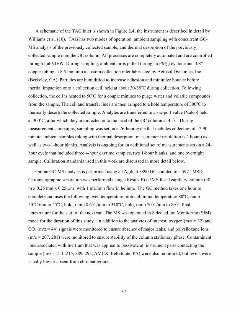
37
A schematic of the TAG inlet is shown in Figure 2.4; the instrument is described in detail by
Williams et al. (10). TAG has two modes of operation: ambient sampling with concurrent GC-
MS analysis of the previously collected sample, and thermal desorption of the previously
collected sample onto the GC column. All processes are completely automated and are controlled
through LabVIEW. During sampling, ambient air is pulled through a PM2.5 cyclone and 3/8”
copper tubing at 8.5 lpm into a custom collection inlet fabricated by Aerosol Dynamics, Inc.
(Berkeley, CA). Particles are humidified to increase adhesion and minimize bounce before
inertial impaction onto a collection cell, held at about 30-35oC during collection. Following
collection, the cell is heated to 50oC for a couple minutes to purge water and volatile compounds
from the sample. The cell and transfer lines are then ramped to a hold temperature of 300oC to
thermally desorb the collected sample. Analytes are transferred to a six-port valve (Valco) held
at 300oC, after which they are injected onto the head of the GC column at 45oC. During
measurement campaigns, sampling was set on a 26-hour cycle that includes collection of 12 90-
minute ambient samples (along with thermal desorption, measurement resolution is 2 hours) as
well as two 1-hour blanks. Analysis is ongoing for an additional set of measurements set on a 24-
hour cycle that included three 4-hour daytime samples, two 1-hour blanks, and one overnight
sample. Calibration standards used in this work are discussed in more detail below.
Online GC-MS analysis is performed using an Agilent 5890 GC coupled to a 5971 MSD.
Chromatographic separation was performed using a Restek Rtx-5MS fused capillary column (30
m x 0.25 mm x 0.25 m) with 1 mL/min flow in helium. The GC method takes one hour to
complete and uses the following oven temperature protocol: initial temperature 80oC, ramp
50oC/min to 45oC, hold; ramp 8.6oC/min to 310oC, hold; ramp 70oC/min to 80oC final
temperature for the start of the next run. The MS was operated in Selected Ion Monitoring (SIM)
mode for the duration of this study. In addition to the analytes of interest, oxygen (m/z = 32) and
CO2 (m/z = 44) signals were monitored to ensure absence of major leaks, and polysiloxane ions
(m/z = 207, 281) were monitored to ensure stability of the column stationary phase. Contaminant
ions associated with Inertium that was applied to passivate all instrument parts contacting the
sample (m/z = 211, 215, 289, 293, AMCX, Bellefonte, PA) were also monitored, but levels were
usually low or absent from chromatograms.

38
TAG was calibrated using liquid standards that are manually injected directly into the
collection cell. Standard #1 contained a mixture of nonpolar and polar analytes of interest
(alkanes, alkanoic acids, PAHs, hopanes, and several of the marker compounds), and was used to
calibrate the MS response and stability via a multipoint calibration at the onset of measurements
and a single-point calibration performed on most subsequent measurement days. Standard #2
contained a mixture of deuterated n-alkanes (C16, C20, C24, C30, C36), n-alkanoic acids (C16,
C18), and cholesterol-d6. This mixture was injected into the collection cell almost daily on top of
collected ambient samples, and instrument response to the deuterated analytes was compared to
injections onto a blank cell in an effort to determine the extent of matrix effects and sample
carryover into subsequent samples. Analysis of this data is ongoing, but the main findings thus
far are (1) similar response for the n-alkanes when spiked in both blank and ambient samples, (2)
much greater response for the alkanoic acids when spiked in ambient samples, suggesting the
organic matrix may partially prevent decomposition of polar compounds during thermal
desorption, and (3) small or negligible carryover (≈10%) into subsequent samples for the
deuterated compounds.
Figure 2.4 Schematic diagrams showing heated zones and flow paths during sampling/analysis mode (left) and thermal desorption mode (right). (From Dr. Nathan Kreisberg, Aerosol Dynamics Inc.)
2.5 Meteorology Measurements
Wind speed and direction data were collected during each intensive study. The county health
department operates a MET station at the Avalon site. There was no MET station at the

39
downtown and urban background (CMU) sites. At these sites measurements from the
Hammerfield site located on Tasso Street in Hazelwood were used to provide regional wind
direction as a function of time. Figure 2.5 shows the location of the Hammerfield site relative to
Diamond Building and Carnegie Mellon University intensive sites.
Figure 2.5 Location of Hammerfield site relative to Diamond Building and Carnegie Mellon University intensive sites.
40
Chapter 3. Spatial Variation in Air Toxic Concentrations and Health Risks
The goal of this chapter is to compare air toxic concentrations and health risks at the four
baseline sites. The spatial variation in air toxic concentrations with the County is assessed and
air toxic concentrations in Allegheny County are compared to national data. Both traditional and
advanced risk models are used to estimate cancer and non-cancer health risks. Risk estimates for
the different sites and for different classes of air toxics are compared. The risk estimates for
Allegheny County are also compared to estimates derived from data collected in other US cities.
Finally, the results of this chapter are used to identify priority air toxics for Allegheny County.
3.2 Methods
3.2.1 Statistical Analysis of Baseline Data
Hypothesis testing, correlation analysis and other statistical techniques were used to compare
air toxics concentrations between sites and to calculate average concentrations for the health risk
assessment. These techniques require knowing the underlying probability distribution of the
concentration data. This distribution is not known, but the Kolmogorov-Smirnov test indicates
that the data varied significantly from the normal distribution. A log normal distribution is often
assumed to calculate upper confidence levels and means of environmental data. However if the
data are skewed compared to traditional log normal models, this approach can significantly
overestimate the upper confidence limit (11).
A bootstrap or re-sampling method provides an alternative approach to estimate confidence
intervals for the means and for hypothesis testing of environmental data (11). The bootstrap
method is a re-sampling technique with replacement. Data is sampled from the original
measurements with replacement and averaged multiple times. The method creates a distribution
of mean values. The confidence interval is determined by finding the 95% of the distribution of
the means. It has been shown that environmental data can be significantly over dispersed
relative to a log-normal distribution (12) and that methods of measuring the upper confidence
limit of the mean based on the log-normal distribution, such as the Land procedure and
Chebyshev’s inequality, can lead to large over estimates of the upper confidence limit of the

41
mean (11, 12). For the rest of this chapter the terms mean or average concentration refers to the
95th percentile upper confidence level of the mean determined using the bootstrap method.
The spatial variability of air toxic concentrations was assessed by comparing study average
concentrations measured at each site. Hypothesis testing was used to determine whether any
differences in study average concentrations were statistically significant. This hypothesis testing
was done using the bootstrap method (11). For hypothesis testing the bootstrap method is used
to determine the means of two data sets and the difference is calculated. This is repeated
multiple times, at least 10,000, to product a distribution of differences in the mean. If 0 was
below the 5th percentile or above the 95th percentile it was assumed that the means of the two
data sets were different.
The spatial variability of air toxics was also assessed using a correlation analysis. For this
analysis, the 24-hour average air toxic concentrations were transformed into log space and the
MATLAB “corr” function was used to determine the correlations between pairs of different
toxics. The p-values for each pair of toxics were then used to test the null hypothesis of no
correlation. If the p-value was greater than 0.05 the null hypothesis could be rejected and the
data were assumed to not be correlated.
3.2.2 Risk Assessment Models
Health risk analyses were performed to estimate lifetime cancer risks, and acute and chronic
non-cancer risks. These estimates were made with both traditional and advance risk models.
The estimates were based on the measured outdoor concentration data from 2006. Outdoor
concentrations provide an estimate of the maximum risks associated with emissions from
outdoor sources.
Since measurements were taken on a one-in-six-day schedule, the sample mean is not
necessarily the same as the long-term average concentration. Therefore, we used the bootstrap
method to determine the mean and the 95th percentile confidence interval of the mean. To
provide a conservative estimate, we use the upper confidence limit on the 95th percentile interval
of the mean to estimate chronic risks.
42
The toxicity data used for the risk assessment were taken from the EPA, CAL EPA, the
Agency for Toxic Substances and Disease Registry, and the DOE Risk Assessment Information
System. These data are summarized in Table 3.1.
3.2.2.1 Traditional Health Risk Models
A linear no-threshold model was used to asses the lifetime cancer risk for 65 air toxics. This
is the standard first-order method of assessing cancer risk (14). The lifetime cancer risk, LIR, for
individual air toxics was determined by
CURELIR * (3.1)
where C is the 95th upper confidence level of the study-average concentration and URE is the
unit risk estimate for the target species. The URE values used for this study are listed in Table
3.1.
If URE data were not available, an estimate was calculated form the oral carcinogenic
potency slope factor as was done in the West Louisville Air Toxics Risk Assessment (15):
BW
IROSFURE
* (3.2)
where OSF is the oral carcinogenic slope factor (mg/kg-day), IR is the inhalation rate (20m3/day)
and BW is the assumed body weight (70 kg).
To quantify non-cancer health risks, the hazard quotient, HQ, was calculated for each of the
measured compounds (14):
RFC
CHQ (3.3)
where C is the 95th percentile upper confidence limit of the study average concentration and RFC
is reference concentration. The hazard index was also determined for each site by adding all of
the HQ values across the set of species at the same location.

43
Table 3.1 Toxicity data for risk analysis.
Chemical Name CAS
Cancer URE (Unit Risk) (1/(g/m3)) Source
Chronic Inhalation
RFC (1/(g/m3)) Source
Systems Targeted by Cancer effects
Systems targeted by non-cancer
effectsModeled in 1996 NATA
Acetaldehyde 75070 2.2E-06 IRIS 9 IRIS Hem,Res X
Acetone 67641 310 ATSDR N
Acrolien 107028 0.02 IRIS Res X
Benzene 71432 7.8E-06 IRIS 60 CAL EPA Hem N X
Benzyl chloride 100447 4.9E-05 IRIS Res
Bromoform 75252 1.1E-06 IRIS 70 Calc Ren,Hep
Bromomethane 74839 5 IRIS Res,N
Butadiene, 1,3- 106990 3.0E-05 IRIS 2 IRIS Hem Res X
Carbon disulfide 75150 710 IRIS
Carbon tetrachloride 56235 1.5E-05 IRIS 40 CAL EPA Hep X
Chlorobenzene 108907 1000 CAL EPA
Chloroethane 75003 10000 IRIS
Chloroform 67663 2.3E-05 IRIS 98 ATSDR Hep,Ren Hep X
Chloromethane 74873 90 IRIS N
Dibromoethane, 1,2- 106934 X
Dichlorobenzene, 1,4- 106467 1.1E-05 CAL EPA 800 IRIS Ren
Dichloroethane, 1,1- 75343 1.6E-05 CAL 500 HEARST Hep,Rep
Dichloroethane,1,2- 107062 2.6E-05 IRIS 2400 ATSDR Rep,Hem,Res X
Dichloroethene, 1,1- 75354 200 IRIS Ren,Hep
Dichloropropane, 1,2- 78875 1.9E-05 Calc 4 IRIS Hep Hep X
Ethyl benzene 100414 1000 IRIS Res,Ren,Hep
Formaldehyde 50000 1.3E-05 IRIS 9.8 IRIS Hem Res X
Hexachlorobutadiene 87683 2.2E-05 IRIS 0.7 Calc Ren X
Hexane 110543 200 IRIS N
Methyl isobutyl ketone 108101 280 Calc
Methylene chloride 75092 4.7E-07 IRIS 1000 ATSDR Hep Hep X
MTBE 1634044 3000 IRIS Ren
Propionaldehyde 123386
Styrene 100425 1000 IRIS N
Tetrachloroethane, 1,1,2,2- 79345 5.8E-05 IRIS&Cal Hep X
Tetrachloroethene 127184 5.9E-06 CAL EPA 270 ATSDR Hep,Ren,Rep,Res N
Toluene 108883 400 IRIS Res,N
Trichlorobenzene, 1,2,4- 120821 200 HEARST
Trichloroethane, 1,1,1- 71556
Trichloroethane,1,1,2- 79005 1.6E-05 IRIS 14 Calc Hep,Ren
Trichloroethene 79016 2.0E-05 CAL EPA 600 CAL EPA Hep,Ren,Rep,Hem N X
Vinyl chloride 75014 8.8E-06 IRIS 100 IRIS Hep,Hem,Res Hep X
Xylene, m/p 108383 100 IRIS N
Xylene, o- 95476 100 IRIS N
Hydrogen Sulfide 647783 2 IRIS Res,N
Organ Systems Toxicity Data Hem: Hematological IRIS: http://www.epa.gov/iris/ Hep: Hepatic Cal EPA: http://www.oehha.org/air/hot_spots/index.html Ren: Renal Calc: Calculated from Equation 3.2 Rep: Reproductive ATSDR: URL: http://www.atsdr.cdc.gov/mrls.html Res: Respiratory HEAST: EPA Health Effect Assessment Summary Tables (13) N: Neurological L: Lymphatic D: Digestive

44
3.2.2.2 Advanced Risk Models
Traditional risk analysis does not account for interaction of pollutants. The EPA (16) has
proposed a model for determining interactive risks based on the work of Mumtaz and Durkin
(17). The EPA model modifies each pollutant’s individual HQ according to its interaction with
each other pollutant in the mixture to define the total interactive hazard for target system/organ p
as (16):
2/)(
*
)(
1,
,
*
1int,
pkpj
pkpj
pjk
n
jpjpadd
pjpadd
pkpjk
n
jk
gpjkBjkjkpjk
n
jpjp
HQHQ
HQHQg
HQHI
HQHI
HQf
MfHQHI
(3.4)
Where:
HQpj = hazard quotient for pollutant j for system p (equation 3.3)
fjk = hazard of the kth pollutant relative to the total additive hazard of all of the
chemicals interacting with pollutant j.
Mjk = interaction magnitude, the EPA has suggested a default of Mjk =5, but Mjk has
been shown to be up to 10 for low dose mixtures (18)
Bjk= weight of evidence that chemical k will effect chemical j’s toxicity. Bjk ranges
from -1 to 0 for antagonistic effects and from 0 to 1 to synergistic effects.
gpik = the degree to which j and k are present in equi-toxic amounts.
The main assumptions of the model are that interactions between pairs of chemicals
contribute the majority of the mixture effect, that synergistic/antagonistic effects are maximized
when two pollutants are present in equal toxicity, that the equation reduces to the additive model
when interactions are minimized, and that adverse health effects of chemical mixtures are limited
to the effects of the individual pollutants. This model also allows for non-symmetric interactions

45
between compounds. For instance, chemical A may have a synergistic effect on chemical B’s
toxicity, but chemical B may have an antagonistic or additive effect on chemical A’s toxicity.
HIint,p values can range from Mjk*HIadd,p to HIadd,p/ Mjk due to the mathematical constraints of the
model.
This interaction model was recently applied by Ryker and Small (18) to evaluate the potential
for interaction among inorganic contaminates in US drinking water. In this project, the model is
used to investigate the potential magnitude of interaction of air toxics. Since there are essentially
no interactions data, this analysis provides only an estimate of the potential interactive health
risks. The results also can be used as a screening tool to identify potentially important
interactions for further research.
To apply the model, pollutants were subdivided into groups based on target systems:
neurological, respiratory, cardiovascular, developmental, skin, hematological, immunological,
reproductive, renal, and hepatic. Three limiting cases were explored for each target system, the
no-interaction condition, the total synergism condition and the total antagonism condition. The
no-interaction condition assumes that all risks are additive (Bjk=0). The total synergism model
assumes that all of the chemicals are interacting to enhance toxicity at the upper limit of
interaction seen in other low-dose mixtures (Mjk =10 and Bjk= 1 for all compounds). This
condition represents a worst case scenario for potential health risk. The total antagonism model
assumes that all of the chemicals are interacting to reduce toxicity with the upper limit of
antagonistic interaction magnitude seen in low-dose mixtures (Mjk =10 and Bjk= -1 for all
compounds). This condition represents a best case scenario for potential health risks from
mixtures.
Similar to previous applications of this interactions model, we use HQ as a measure of non-
cancer equi-toxicity. As previously stated, non-cancer HQ values are not directly comparable
between pollutants because the RfC is related to differing levels of toxicity. The differences in
toxicity associated with HQ values add a level of uncertainty to the interactive analysis but
should not greatly affect the prioritizing of interactions for research priorities.
Although the interaction model was developed to explore non-cancer risks, it can be adapted
to be applied to cancer risks as well. EPA proposed a method for translating the LIR to a hazard
quotient for a given cancer risk threshold by normalizing exposure, E, by a dose associated with
46
a given risk level, DR, which is equivalent to the previously calculated LIR normalized by a
cancer risk threshold, RT. The equivalent cancer hazard quotient of a pollutant n would be (16):
RTLIRDREHQ nnnn // (3.5)
The potential synergistic/antagonistic hazard indices and cancer LIR for each of the target
systems were calculated for systems that had two or more measured pollutants that affected it. In
addition to the volatile organic air toxics, non-cancer interactions with manganese hydrogen
sulfide were also explored. The manganese data were from an urban background site, and the
hydrogen sulfide analysis was performed using the data from the Avalon site.
3.3 Air Toxic Concentrations in Allegheny County
Table 3.2 summarizes the air toxic concentrations measured during the baseline sampling.
To illustrate the temporal variability of the data, the table lists the geometric mean, median,
standard deviation, 95th, 75th, median, 25th, and 5th percentile of the 24-hr concentrations
measured at each baseline site. Average concentrations at each baseline site are plotted in
Figures 3.1a and 3.2a.
Daily air toxics concentrations at the four baseline sites ranged from below detection limit to
24.4 ppbv. Concentrations of some toxics such as carbon tetrachloride exhibited little temporal
or spatial variability. Others exhibited significant temporal and/or spatial variability. Toluene,
acetone, formaldehyde and benzene had the highest one-day concentration spikes at all sites
except downtown where there were large spikes in methylene chloride. As discussed below,
these temporal and spatial patterns provide insight into pollutant sources.

47
Table 3.2 Summary of baseline air toxic concentrations in pptv
FLAG PLAZA SOUTH FAYETTE
Chemical Name Mea
n
Med
ian
5th
per
cen
tile
25th
per
cen
tile
75th
per
cen
tile
95th
Per
cen
tile
Sta
nd
. Dev
.
Mea
n
Med
ian
5th
per
cen
tile
25th
per
cen
tile
75th
per
cen
tile
95th
Per
cen
tile
Sta
nd
. Dev
.
Acetaldehyde 1000 950 380 630 1260 2000 470 800 790 440 630 950 1270 270Acrolein 55 40 3 25 64 170 58 35 31 7 20 46 72 20Benzene 420 340 160 220 550 850 270 330 210 80 150 340 600 470Benzyl Chloride 5 0 0 0 10 20 7 3 0 0 0 0 11 6Bromoform 1 0 0 0 0 10 2 1 0 0 0 0 0 2Bromomethane 10 10 0 10 10 20 6 8 10 0 8 10 11 5Butadiene,1,3- 65 50 10 30 90 160 55 22 10 0 0 30 72 32Carbon disulfide 69 20 10 20 40 260 180 35 20 10 20 60 71 27Carbon tetrachloride 84 80 70 80 90 110 11 85 80 70 80 90 100 12Chlorobenzene 1 0 0 0 0 10 4 3 0 0 0 10 10 5Chloroethane 7 0 0 0 10 20 17 4 0 0 0 10 10 5Chloroform 27 20 10 20 30 40 12 18 20 10 10 20 21 6Chloromethane 640 630 540 580 690 760 72 570 560 490 530 610 690 66Dibromoethane,1,2- 0 0 0 0 0 0 2 0 0 0 0 0 0 2Dichlorobenzene,1,4- 130 110 60 80 150 240 60 11 10 0 10 10 20 6Dichloroethane,1,1- 1 0 0 0 0 10 3 1 0 0 0 0 0 2Dichloroethane,1,2- 9 10 0 10 10 20 6 8 10 0 10 10 10 4Dichloroethene,1,1- 1 0 0 0 0 10 4 1 0 0 0 0 10 3Dichloropropane,1,2- 1 0 0 0 0 10 2 2 0 0 0 0 10 4Ethylbenzene 100 70 40 50 130 260 71 39 30 10 20 43 81 27Formaldehyde 1700 1270 490 840 2470 3590 1130 1690 1310 580 990 2220 3500 1170Hexachloro-1,3-Butadiene 4 0 0 0 10 10 5 5 0 0 0 10 10 6Hexane 200 140 60 100 250 500 170 99 90 40 60 120 180 48Methyl Isobutyl Ketone 32 20 0 0 40 80 45 26 20 0 0 43 61 27Methylene Chloride 220 110 70 80 140 500 430 69 60 50 60 80 110 25MTBE 11 10 0 0 20 30 20 6 0 0 0 10 11 8Propionaldehyde 320 250 80 170 380 790 220 270 220 130 170 350 570 160Styrene 34 20 10 10 40 100 36 19 15 0 10 20 41 21Tetrachloroethane,1,1,2,2- 1 0 0 0 0 10 3 1 0 0 0 0 0 2Tetrachloroethylene 38 30 10 20 50 100 27 14 10 0 10 20 31 10Toluene 850 520 230 380 970 1920 1080 510 400 90 240 590 990 620Trichlorobenzene,1,2,4- 3 0 0 0 10 10 6 4 0 0 0 10 11 6Trichloroethane,1,1,1- 25 20 20 20 30 40 12 16 15 10 10 20 21 6Trichloroethane,1,1,2- 1 0 0 0 0 10 2 0 0 0 0 0 0 0Trichloroethene 110 20 0 10 85 620 190 5 0 0 0 10 10 6Vinyl Chloride 1 0 0 0 0 10 3 0 0 0 0 0 0 2Xylene, m/p- 300 230 100 140 430 710 220 100 75 30 58 110 250 95Xylene, o- 110 80 40 50 150 270 80 40 30 10 20 50 100 33

48
Table 3.2 (continued) Summary of baseline air toxic concentrations in pptv
\
STOWE AVALON
Chemical Name Mea
n
Med
ian
5th
per
cen
tile
25th
per
cen
tile
75th
per
cen
tile
95th
Per
cen
tile
Sta
nd
. Dev
.
Mea
n
Med
ian
5th
per
cen
tile
25th
per
cen
tile
75th
per
cen
tile
95th
Per
cen
tile
Sta
nd
. Dev
.
Acetaldehyde 1030 850 410 670 1280 1960 550 1120 970 600 730 1300 2180 500Acrolein 65 60 10 28 84 140 56 72 62 17 49 100 160 50Benzene 520 360 130 230 530 1330 470 730 610 180 320 1010 1460 580Benzyl Chloride 2 0 0 0 0 10 4 3 0 0 0 10 10 6Bromoform 0 0 0 0 0 0 0 0 0 0 0 0 0 2Bromomethane 9 10 0 5 10 20 6 9 10 0 10 10 20 6Butadiene,1,3- 42 30 10 20 50 110 41 70 50 10 30 80 150 69Carbon disulfide 29 20 10 15 30 69 21 33 20 10 20 40 88 26Carbon tetrachloride 82 80 70 80 90 100 13 83 80 70 80 90 98 9Chlorobenzene 2 0 0 0 0 10 4 2 0 0 0 0 10 5Chloroethane 11 10 0 0 10 29 13 3 0 0 0 10 10 5Chloroform 19 20 10 10 20 30 8 25 20 10 20 30 48 10Chloromethane 590 560 500 530 650 700 79 580 570 480 540 620 680 64Dibromoethane,1,2- 0 0 0 0 0 0 0 0 0 0 0 0 0 0Dichlorobenzene,1,4- 20 20 1 10 30 40 12 23 20 10 10 30 50 16Dichloroethane,1,1- 0 0 0 0 0 0 0 0 0 0 0 0 0 1Dichloroethane,1,2- 8 10 0 10 10 10 5 8 10 0 10 10 10 5Dichloroethene,1,1- 0 0 0 0 0 0 2 0 0 0 0 0 0 2Dichloropropane,1,2- 0 0 0 0 0 0 2 1 0 0 0 0 8 2Ethylbenzene 130 60 30 40 110 440 210 120 95 43 80 130 250 72Formaldehyde 1670 1250 430 930 2470 3300 1080 2110 1720 960 1200 2780 4140 1190Hexachloro-1,3-Butadiene 3 0 0 0 10 10 5 3 0 0 0 10 10 5Hexane 150 110 51 70 170 370 120 200 170 73 110 220 390 130Methyl Isobutyl Ketone 34 30 0 10 50 79 29 53 40 0 0 78 180 61Methylene Chloride 95 80 60 70 100 170 42 100 90 60 70 120 200 45MTBE 8 0 0 0 10 30 10 11 10 0 0 20 28 11Propionaldehyde 320 240 130 170 420 710 210 340 270 150 210 440 690 180Styrene 78 50 20 30 80 220 100 110 100 20 60 160 240 69Tetrachloroethane,1,1,2,2- 0 0 0 0 0 0 0 0 0 0 0 0 0 1Tetrachloroethylene 30 20 10 10 35 89 28 55 30 10 20 40 120 110Toluene 680 540 210 390 880 1700 450 980 770 390 560 1290 2120 580Trichlorobenzene,1,2,4- 3 0 0 0 5 10 5 5 0 0 0 10 10 6Trichloroethane,1,1,1- 15 20 10 10 20 20 5 17 20 10 10 20 20 5Trichloroethane,1,1,2- 0 0 0 0 0 0 0 0 0 0 0 0 0 0Trichloroethene 6 0 0 0 10 20 9 7 10 0 0 10 18 7Vinyl Chloride 0 0 0 0 0 0 0 0 0 0 0 0 0 1Xylene, m/p- 270 170 61 100 330 780 260 360 290 120 200 400 870 250Xylene, o- 120 80 21 45 130 310 110 150 120 53 90 180 340 90
3.3.1 Spatial Variation in Gas Phase Air Toxic Concentrations
One of the main goals of this project was to quantify the spatial variability of air toxic
concentrations throughout Allegheny County. Of particular interest was to compare
concentrations at the heavily urbanized sites (Avalon, Stowe, and Flag Plaza) to those in the
regional background (South Fayette). Such a comparison provides insight into the influence of
local sources on human exposure.

49
We quantified the spatial variability by calculating ratios of the study average concentrations
at each urban site to those in South Fayette. These concentration ratios are plotted in Figures
3.1b and 3.2b. Air toxics with concentration ratios greater than one indicate significant influence
of local emissions.
Figures 3.1b and 3.2b indicate that average concentrations of 12 of the air toxics varied by
less than 25% across the four baseline sites (concentration ratios less than 1.25), indicating little
spatial variation in average concentrations. These 12 are 1,2-dichloropropane, 1,2-
dibromomethane, bromoform, hexachlorobutadiene, chlorobenzene, bromomethane, 1,2-
dichloroethane, 1,2,4-trichlorobenzene, chloromethane, carbon tetrachloride, formaldehyde and
propionaldehyde. Of these 12, hypothesis testing indicates that the differences in average
concentrations between sites of only one toxic, formaldehyde, were statistically significant. The
average formaldehyde concentrations in Avalon appear to be 20% higher than those at the other
sites. Correlation analysis was also performed to assess the regionality of these air toxics. A
regional toxic is one in whose concentration at one site is more strongly correlated with the same
toxic at other sites than with other pollutants at the same site. This correlation analysis showed
that there may be modest local emissions of some these 12 toxics at Stowe and Avalon, but that
these local emissions do not have a large effect on concentrations.
Concentrations of 27 air toxics were more than 25% higher at one or more of the urban sites
compared to South Fayette, indicating some influence of local sources. Twelve of these toxics
had moderate concentrations ratios between 1.25 and 2. This included 1,1 dichloroethane, 1,1,2-
trichloroethane, 1,1,-dichloroethene, 1,1,2,2-tetrachloroethane, MTBE, 1,1,1-trichloroethane,
benzyl chloride, chloroform, methyl isobutyl ketone, acetaldehyde, toluene and benzene.
Average concentrations of 15 of the 39 air toxics measured during the baseline study were a
factor of two higher or more higher at one of the urban sites compared to South Fayette,
indicating strong effects of local sources. These 15 are vinyl chloride, chloroethane, acrolein,
hexane, 1,3-butadiene, carbon disulfide, m/p-xylene, o-xylene, tetrachloroethene, ethyl benzene,
methylene chloride, styrene, 1,4-dichlorobenzene, trichloroethene.
Chlorinated compounds at the Flag Plaza site had the largest concentration ratios; for
example, study average trichloroethylene and 1,4-dichlorobenzene concentrations were 26 and
12 times higher downtown compared to South Fayette, respectively. Concentrations of many air
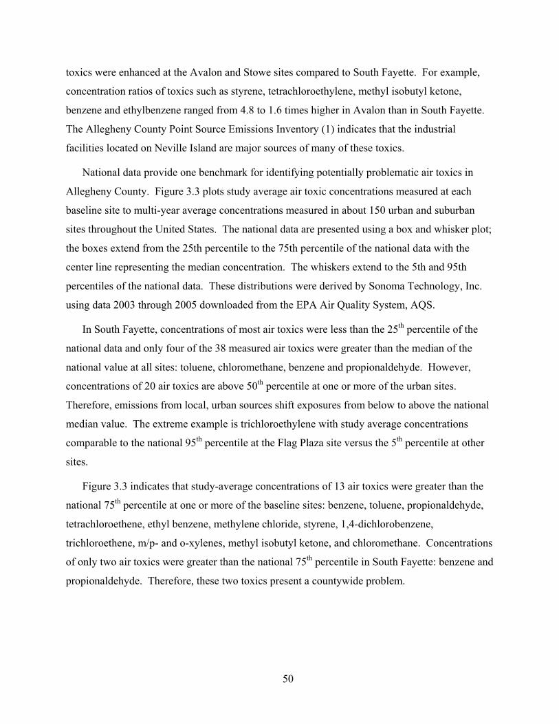
50
toxics were enhanced at the Avalon and Stowe sites compared to South Fayette. For example,
concentration ratios of toxics such as styrene, tetrachloroethylene, methyl isobutyl ketone,
benzene and ethylbenzene ranged from 4.8 to 1.6 times higher in Avalon than in South Fayette.
The Allegheny County Point Source Emissions Inventory (1) indicates that the industrial
facilities located on Neville Island are major sources of many of these toxics.
National data provide one benchmark for identifying potentially problematic air toxics in
Allegheny County. Figure 3.3 plots study average air toxic concentrations measured at each
baseline site to multi-year average concentrations measured in about 150 urban and suburban
sites throughout the United States. The national data are presented using a box and whisker plot;
the boxes extend from the 25th percentile to the 75th percentile of the national data with the
center line representing the median concentration. The whiskers extend to the 5th and 95th
percentiles of the national data. These distributions were derived by Sonoma Technology, Inc.
using data 2003 through 2005 downloaded from the EPA Air Quality System, AQS.
In South Fayette, concentrations of most air toxics were less than the 25th percentile of the
national data and only four of the 38 measured air toxics were greater than the median of the
national value at all sites: toluene, chloromethane, benzene and propionaldehyde. However,
concentrations of 20 air toxics are above 50th percentile at one or more of the urban sites.
Therefore, emissions from local, urban sources shift exposures from below to above the national
median value. The extreme example is trichloroethylene with study average concentrations
comparable to the national 95th percentile at the Flag Plaza site versus the 5th percentile at other
sites.
Figure 3.3 indicates that study-average concentrations of 13 air toxics were greater than the
national 75th percentile at one or more of the baseline sites: benzene, toluene, propionaldehyde,
tetrachloroethene, ethyl benzene, methylene chloride, styrene, 1,4-dichlorobenzene,
trichloroethene, m/p- and o-xylenes, methyl isobutyl ketone, and chloromethane. Concentrations
of only two air toxics were greater than the national 75th percentile in South Fayette: benzene and
propionaldehyde. Therefore, these two toxics present a countywide problem.

51
0.01 0.1 1Mean Concentration (g/m3)
Trichloroethene
Dichlorobenzene, 1,4-
Styrene
Tetrachloroethene
Methylene chloride
Ethyl benzene
Xylene, o-
Xylene, m-
Butadiene, 1,3-
Chloroethane
Carbon disulfide
Hexane
Vinyl chloride
Acrolien
Methyl isobutyl ketone
MTBE
Benzene
Toluene
Trichloroethane,1,1,1-
Chloroform
South Fayette Flag Plaza Stowe Avalon
81
2 3 4 5 6 7 810
2
Concentration Normalized by South Fayette
Flag Plaza Stowe Avalon
Figure 3.1. (a) Study-average air toxic concentrations measured at the four baseline sites. (b) Ratio of study average concentrations measured at the three urban baseline sites to those measured in South Fayette. Ratios greater than one indicate that concentrations at the urban site are greater than those in South Fayette.
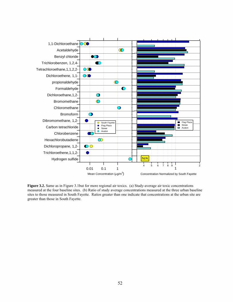
52
0.01 0.1 1
Mean Concentration (g/m3)
1,1-Dichloroethane
Acetaldehyde
Benzyl chloride
Trichlorobenzen, 1,2,4-
Tetrachloroethane,1,1,2,2-
Dichloroethene, 1,1-
propionaldehyde
Formaldehyde
Dichloroethane,1,2-
Bromomethane
Chloromethane
Bromoform
Dibromomethane, 1,2-
Carbon tetrachloride
Chlorobenzene
Hexachlorobutadiene
Dichloropropane, 1,2-
Trichloroethene,1,1,2-
Hydrogen sulfide
South Fayette Flag Plaza Stowe Avalon
4 5 6 7 8 91
2
Concentration Normalized by South Fayette
Flag Plaza Stowe Avalon
N/A
Figure 3.2. Same as in Figure 3.1but for more regional air toxics. (a) Study-average air toxic concentrations measured at the four baseline sites. (b) Ratio of study average concentrations measured at the three urban baseline sites to those measured in South Fayette. Ratios greater than one indicate that concentrations at the urban site are greater than those in South Fayette.

53
Figure 3.3. Comparison of study-average concentrations measured at the four baseline sites to national air toxic data. The national data are multi-year average concentrations measured at about 150 urban and suburban sites throughout the United States; these data are presented using a box and whisker plot. The boxes extend from the 25th percentile to the 75th percentile of the national data with the center line representing the median concentration. The whiskers extend to the 5th and 95th percentiles of the national data.

54
3.3.2 Diesel Particulate Matter (DPM)
Diesel particulate matter (DPM) is a complex mixture of elemental carbon (EC), organic
carbon (OC), sulfate, nitrate, and trace metals and ions. EC and OC comprise most of the
emissions on a mass basis. Because of the inherent complexity of DPM, as well as potential
contributions of these PM species by other sources, it is impossible to directly measure DPM
concentrations. Instead DPM concentrations must be inferred using a source apportionment
model. The measurements of BC and condensed phase molecular markers at the Diamond
Building were used to estimate DPM concentrations in downtown area. Similar analysis was
performed using archived data to estimate DPM concentrations in Schenley Park. These
analyses are described in detail in Chapter 6; here we summarize the results which are used in
the risk assessment. Average DPM concentrations at the Diamond Building were estimated to be
3.6 g/m3 versus 0.6 g/m3 in Schenley Park. Therefore, there are significant spatial variations
in DPM concentrations in Allegheny County.
To further assess the spatial variation of DPM in the Pittsburgh Area, Figure 3.4 compares
average BC concentrations measured at six sites in and around the Allegheny County. BC
contributes roughly half of the DPM and, therefore, provides a reasonable proxy for DPM
exposures. Archived BC data were available for Schenley Park, Hazelwood, Lawrenceville,
Florence and Greensburg. At the Diamond Building, BC levels were about four times higher
than at any of the other Pittsburgh area sites. Therefore, the downtown area is a DPM hotspot,
which is not surprising given the high density of diesel vehicles in the area (buses, trucks, and
construction equipment). BC levels at the other four urban sites are very similar, about 0.6 g m-
3. The relative contribution of local sources can be estimated by comparing BC concentrations in
Pittsburgh to data from Florence, a rural site in Washington County that is generally upwind of
the city. Except at the Diamond Building, BC concentrations at the other Pittsburgh sites were
only about 50% higher than in Florence. Therefore, about two-thirds of the BC outside of the
downtown area comes from regional transport, which implies that a substantial fraction of the
DPM outside of the downtown area comes from regional transport. However, local emissions
dominate DPM exposures at the Diamond Building.
Figure 3.4 also presents BC data from fifteen other urban and rural locations in the United
States. These data were collected during the summertime in 2001 through 2004 by the EPA

55
Speciation Trends Network. Data from multiple sites in Chicago and New York City are shown
to illustrate the spatial variation of BC in urban areas. Except for the Diamond Building, BC
concentrations at the three other city of Pittsburgh sites (Hazelwood, Lawrenceville, and
Schenley Park) are at or below concentrations in other US cities. The BC concentrations at the
Diamond Building are the highest of any of the sites, comparable to measurements made in
Elizabeth NJ near exit 13 of the New Jersey Turnpike. However, it is not known how
representative the BC measurements made at the Diamond Building are of the larger downtown
area. The Diamond Building is located at the intersection of Fifth and Liberty Avenues; both of
these streets are major bus thoroughfares.
0 0.5 1 1.5 2 2.5
St Louis
Chicago Site 3
Chicago Site 2
Chicago Site 1
Detroit Site 2
Detroit Site 1
Elizabeth, NJ
Downtown Manhattan
Bronx, NY
Queens, NY
Boston
Baltimore
Rural MI
Rural NJ
Rural PA
Diamond Building
Hazelwood
Lawrenceville
Schenley Park
Greensburg
Florence
BC or EC (g/m3)
DATA FROM PITTSBURGH AREA
DATA FROM OTHER LOCATIONS
Figure 3.4. Average BC or EC concentrations at monitoring sites in and around Allegheny County and in other locations in the United States. Downtown measurements were made during the 2008 intensive at the Diamond Building; the data from the other Pittsburgh area sites were measured in 2001 and 2002 during the Pittsburgh Air Quality Study; the data from the other locations are averages of measurements collected as part of the EPA Speciation Trends Network (STN) during June, July and August of 2001 through 2004.

56
3.4 Risk Analysis
Although air toxic concentrations provide a measure of exposure, health risks depend on both
the concentration and the toxicity of a pollutant. Since the toxicity of air pollutants can vary
widely, one can draw misleading conclusions if one only considers the concentration data. In this
section we present results from health risk analysis performed using both the high time resolved
and 24-hour average data using both traditional and advanced health risk models.
3.4.1 Cancer Risks of Gas Phase Organic Air Toxics
The LIR calculated for the organic air toxics measured during the baseline study are shown
in Figure 3.5. At present there are no risk levels that represent acceptable or unacceptable
regulatory thresholds for air toxics. However, EPA has made case-specific determinations such
as the 1989 Benzene National Emission Standard for Hazardous Air Pollutants (NESHAP) that
set up a two-part risk-based decision framework
(http://www.epa.gov/ttn/atw/nata/natsafaq.html). First, it set an upper limit of acceptability of 1
in 10,000 lifetime cancer risk for highly exposed individuals. Second, it set a target of protecting
the greatest number of persons possible to an individual lifetime risk level no higher than
approximately 1 in 1,000,000.
Of the organic air toxics considered in this study, 11 present cancer risks above the 10-6
threshold with three above 10-5 at one or more of the sites. The three toxics above the 10-5
threshold are (in order of decreasing risk) formaldehyde, benzene, and trichloroethylene. The
remaining eight that are above the 10-6 threshold are 1,4-dichlorobenzene, carbon tetrachloride,
1,3-butadiene, acetaldehyde, tetrachloroethene, chloroform, hexachlorobutadiene, benzyl
chloride, and 1,2-dichloroethane. None of the organic air toxics are estimated to pose a risk
greater than 10-4.
Figure 3.5 indicates that the variation in LIR is much more pollutant dependent than site
dependent. In other words, the cancer risks were largely driven by the same set of compounds at
all of the sites because the pollutant-to-pollutant differences in toxicity are much greater than the
site-to-site differences in concentrations. The exceptions to this trend are trichloroethylene and
1,4-dichlorobenzene, which pose substantially greater risk at the Flag Plaza site than at the other
sites.

57
To compare the overall cancer risk posed by organic air toxics at the four baseline sites,
Figure 3.6 plots the additive LIR. Although concentrations of six air toxics were at least a factor
of two higher at the Stowe and Avalon sites, Figure 3.6 indicates that the additive cancer risks at
these sites were only 25% greater than the estimated risk in South Fayette, mostly due to higher
benzene concentrations. Organic air toxics pose the greatest cancer risk at the Flag Plaza site
where concentrations of eight toxics were greater than a factor of two higher and concentrations
of two toxics were more than a factor of ten higher than conditions in South Fayette. However,
the additive cancer risk at Flag Plaza was only 50% higher than in the South Fayette. At the
downtown site, trichloroethene and 1,4 dichlorobenzene significantly contribute to the cancer
risk. At this site they accounted for 26% of the estimated cancer risk but only 2-3% of the risks
at the other sites.
Why is the spatial variation in the additive cancer risk so small? Figure 3.6 indicates that two
regionally distributed air toxics (formaldehyde and carbon tetrachloride) contribute about half of
the total risk. Therefore, incremental additional risk caused by air toxics with elevated
concentrations at one or more of the urban sites was relatively small.
Figure 3.7 shows the additive LIR for different organ systems with a risk larger than 10-6.
The greatest cancer risks for each site were found to be for the hematological systems. The
chlorinated compounds increased risks of renal, hepatic and reproductive cancer at the
downtown site.

58
10-8
10-7
10-6
10-5
Cancer LIR (Lifetime Individual Risk)
Formaldehyde
Benzene
Carbon tetrachloride
Acetaldehyde
Butadiene, 1,3-
Chloroform
Dichlorobenzene,1,4-
Tetrachloroethene
Dichloroethane, 1,2-
Hexachlorobutadiene
Trichloroethene
Benzyl chloride
Methylene chloride
Dichloropropane, 1,2-
Tetrachloroethane,1,1,2,2-
Dichloroethane,1,1-
Trichloroethane,1,1,2-
Vinyl chloride
Bromoform
South Fayette Flag Plaza Stowe Avalon
Figure 3.5. Cancer lifetime incidence rate, LIR, calculated using the study upper limit of the 95% confidence interval of the study-average concentration. The vertical red dashed line indicates a risk of 10-6 of (1 in a million).

59
Figure 3.6 Additive cancer lifetime incidence rate, LIR, posed by the 38 gas-phase organic air toxics measured at the four baseline sites.
NATA and previous air toxic studies in other areas of the country have identified
acrylonitrile as a potential risk. Acrylonitrile was only measured for 6 months of 2008 at the
Flag Plaza site. The 95th percentile upper confidence limit on the mean of these data was 0.064
g/m3. This is between the 10th and 20th national percentile for acrylonitrile. The cancer LIR
would be 4.4 x 10⁻⁶ and the HQ would be 0.032.
3.4.2 Non-Cancer Risks of Gas Phase Organic Air Toxics
Chronic non-cancer HQs are shown in Figure 3.8. The hazard quotient is thought to be
proportional to risk, but is not a direct measure of the probability of disease like the LIR (19).
Therefore HQ provides a binary indication of risk: values less then 1 are considered non-
hazardous, while values of 1 or greater indicate that there is potential for an elevated non-cancer
risk. It also indicates how much ambient concentrations must be reduced to achieve a “safe”
level.
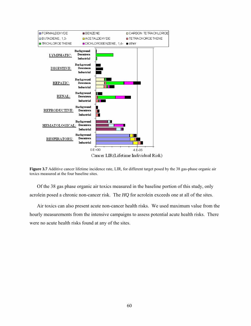
60
Figure 3.7 Additive cancer lifetime incidence rate, LIR, for different target posed by the 38 gas-phase organic air toxics measured at the four baseline sites.
Of the 38 gas phase organic air toxics measured in the baseline portion of this study, only
acrolein posed a chronic non-cancer risk. The HQ for acrolein exceeds one at all of the sites.
Air toxics can also present acute non-cancer health risks. We used maximum value from the
hourly measurements from the intensive campaigns to assess potential acute health risks. There
were no acute health risks found at any of the sites.

61
10-5
10-4
10-3
10-2
10-1
100
101
Hazard Quotient
AcrolienFormaldehydeAcetaldehyde
Butadiene, 1,3-Hexachlorobutadiene
BenzeneXylene,m/p-
ChloromethaneCarbon tetrachloride
TolueneBromomethane
Xylene,o-Hexane
TetrachloroetheneDichloropropane,1,2-
ChloroformMethyl isobutyl ketone
StyreneEthyl benzene
Methylene chlorideTrichlorobenzene,1,2,4-
Dichlorobenzene,1,4-Carbon disulfide
BromoformTrichloroethene
Dichloroethene,1,1-MTBE
Vinyl chlorideDichloroethane,1,2-
ChlorobenzeneChloroethane
South Fayette Flag Plaza Stowe Avalon
Figure 3.8 Hazard quotients (HQ) for non-cancer chronic health effects. The dashed vertical red line indicates a HQ of one. Air toxics with a HQ less than one are thought not to pose a non-cancer risk.
3.4.3 Diesel Particulate Matter Health Risks
Cancer and chronic non-carcinogenic risks of diesel particulate matter were estimated for the
Diamond Building and Schenley Park. Although diesel particulate mater is thought to be a
human carcinogen, EPA did not report quantitative cancer risk estimates for diesel particulate
matter as part of the National Air Toxic Assessment (NATA) because of uncertainty in the diesel
particulate matter toxicity data (i.e., unit risk estimate or URE). To assess carcinogenic risk, we
applied a risk potency factor of 3 x 10⁻⁴ per g m-3 DPM recommended by California’s Office of
Environmental Health Hazard Assessment (OEHHA). OEHHA estimates an overall range of
lung cancer risk factors of (1.3 – 15) x 10-4 per g m-3 for DPM, indicating that associated risk is
subject to uncertainty of about an order of magnitude.
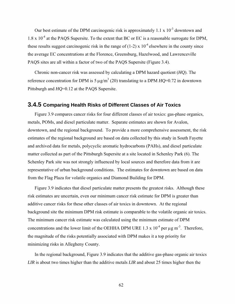
62
Our best estimate of the DPM carcinogenic risk is approximately 1.1 x 10⁻³ downtown and
1.8 x 10⁻⁴ at the PAQS Supersite. To the extent that BC or EC is a reasonable surrogate for DPM,
these results suggest carcinogenic risk in the range of (1-2) x 10-4 elsewhere in the county since
the average EC concentrations at the Florence, Greensburg, Hazelwood, and Lawrenceville
PAQS sites are all within a factor of two of the PAQS Supersite (Figure 3.4).
Chronic non-cancer risk was assessed by calculating a DPM hazard quotient (HQ). The
reference concentration for DPM is 5 g/m3 (20) translating to a DPM HQ=0.72 in downtown
Pittsburgh and HQ=0.12 at the PAQS Supersite.
3.4.5 Comparing Health Risks of Different Classes of Air Toxics
Figure 3.9 compares cancer risks for four different classes of air toxics: gas-phase organics,
metals, POMs, and diesel particulate matter. Separate estimates are shown for Avalon,
downtown, and the regional background. To provide a more comprehensive assessment, the risk
estimates of the regional background are based on data collected by this study in South Fayette
and archived data for metals, polycyclic aromatic hydrocarbons (PAHs), and diesel particulate
matter collected as part of the Pittsburgh Supersite at a site located in Schenley Park (6). The
Schenley Park site was not strongly influenced by local sources and therefore data from it are
representative of urban background conditions. The estimates for downtown are based on data
from the Flag Plaza for volatile organics and Diamond Building for DPM.
Figure 3.9 indicates that diesel particulate matter presents the greatest risks. Although these
risk estimates are uncertain, even our minimum cancer risk estimate for DPM is greater than
additive cancer risks for these other classes of air toxics in downtown. At the regional
background site the minimum DPM risk estimate is comparable to the volatile organic air toxics.
The minimum cancer risk estimate was calculated using the minimum estimate of DPM
concentrations and the lower limit of the OEHHA DPM URE 1.3 x 10⁻⁴ per g m-3. Therefore,
the magnitude of the risks potentially associated with DPM makes it a top priority for
minimizing risks in Allegheny County.
In the regional background, Figure 3.9 indicates that the additive gas-phase organic air toxics
LIR is about two times higher than the additive metals LIR and about 25 times higher then the

63
additive PAH LIR. At Avalon, the risk posed by metals is about a factor of three lower than that
posed by volatile organic air toxics.
Figure 3.9 Comparison of additive cancer risk for different classes of air toxics. The estimates for the regional background are based on data from the South Fayette site collected as part of this study (volatile organics) and archived data from the Pittsburgh Supersite in Schenley Park (PAH, metals, and diesel PM).
Figure 3.10 compares non-cancer hazard quotients of air toxics for metals, DPM, and
hydrogen sulfide. Metals do not appear to pose a significant non-cancer risk. All of the metals
measured at the regional background site were more than a factor of ten less then their respective
RfC values with the exception of manganese which was more than a factor of five less then it’s
RfC value. Figure 3.11 shows that there is little spatial variation in metal hazard quotients
around Allegheny County. At all sites the additive metals hazard index is lower than 0.8.
Although no longer classified as an air toxic, hydrogen sulfide is a by product of coke plants
that affects respiratory and neurological health (21). Figure 3.10 indicates that hydrogen sulfide
does present a potential non-cancer risk at Avalon. It is uncertain how hydrogen sulfide
contributes to health risks elsewhere in the county since it is not routinely measured at locations
not immediately adjacent to large coke works.
10-6
10-5
10-4
10-3
Ca
nce
r L
IR
RegionalDowntownAvalon
No
Met
als
Dat
a
No
PA
H D
ata
No
DP
M D
ata
No
PA
H D
ata
Die
sel P
M
Die
sel P
M
Vo
latil
e O
rga
nic
s
Vo
latil
e O
rga
nic
s
Vo
latil
e O
rgan
ics
Met
als
Me
talsPA
H

64
0.001 0.01 0.1 1 10
Acrolien (Avalon)Acrolien (Stowe)
Acrolien (Downtown)Acrolien (South Fayette)
Hydrogen Sulfide (Avalon)DPM (Downtown)
Manganese (Avalon)Manganese (Regional
DPM (Regional Background)Arsenic (Avalon)
Cadmium (Avalon)Arsenic (Regional Background)Mercury (Regional Background)
Cadmium (Regional Background)Chromium (Regional Background)
Chromium (Avalon)Nickel (Avalon)
Nickel (Regional Background)Beryllium (Regional Background)
Hazard Quotient
Figure 3.10 Comparison of hazard quotients for different classes of air toxics measured at regional background sites. The dashed line represents a hazard quotient of 1 indicating potential for non-cancer risks and a hazard quotient of .1, an indicator that concentrations being a factor of ten less then their RfC value.
0.80.60.40.2
Hazard Quotient
Avalon
Lawrenceville
Hazelwood
Florence
Greensburg
Schenley Park Arsenic Cadmium Chromium Manganese Nickel
Figure 3.11 Non-cancer hazard quotients of metals calculated using archived data (6). The Schenley Park site is the urban background site.

65
3.4.6 Comparison of Risks in different U.S. Cities
Figure 3.12 compares the additive cancer risk posed by the 38 gas-phase organic air toxics at
the four baseline sites in Allegheny County to estimates for 14 other United States cities. The
risk estimates for the other cities are based on annual average concentrations for the same set of
air toxics using data from 2006 that are archived in the EPA AQS (22).
Figure 3.12 indicates that the estimated risks vary by less than a factor of three across the set
of cities, with the lowest risk being estimated for San Francisco and the highest risk in Detroit.
Allegheny County falls within the middle two quartiles of this distribution. Therefore, the risks
in Allegheny are comparable to those in other US cities.
Figure 3.12 also illustrates the similarity in the risk profiles between the cities. The toxics
that are driving the health risks in Allegheny County are largely the same as those posing the
risks elsewhere in the United States.
Figure 3.13 compares the additive LIR for metals measured in Allegheny County and six
different cities. The metal risks for Allegheny County were estimated using archived data from
the six sites in and around Allegheny County. Most of the archived data were collected as part
of the Pittsburgh Supersite during 2001 and 2002. The analysis also used more recent metals
data taken at Avalon.
The comparison reveals that the cancer risk posed by metals in Allegheny County are
comparable to those in other US cities. The metals risks in Allegheny County are somewhat
greater than those in Seattle, Boston, Portland, and Washington DC, but significantly less than
the risks of metals in Tampa and Houston.

66
Figure 3.12 Comparison of additive cancer risks at the four baseline sites in Allegheny County to other cities in the United States. The comparisons are based on the 38 organic gas-phase air toxics considered in this study.
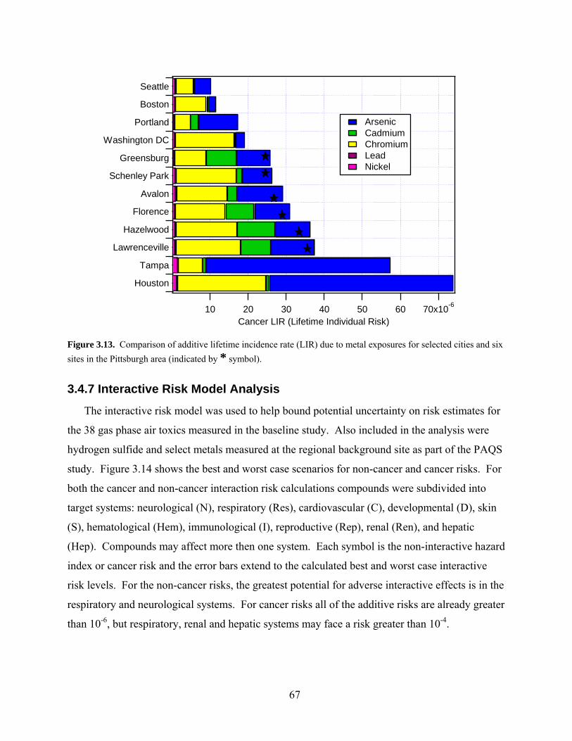
67
70x10-6
605040302010Cancer LIR (Lifetime Individual Risk)
Seattle
Boston
Portland
Washington DC
Greensburg
Schenley Park
Avalon
Florence
Hazelwood
Lawrenceville
Tampa
Houston
Arsenic Cadmium Chromium Lead Nickel
Figure 3.13. Comparison of additive lifetime incidence rate (LIR) due to metal exposures for selected cities and six
sites in the Pittsburgh area (indicated by * symbol).
3.4.7 Interactive Risk Model Analysis
The interactive risk model was used to help bound potential uncertainty on risk estimates for
the 38 gas phase air toxics measured in the baseline study. Also included in the analysis were
hydrogen sulfide and select metals measured at the regional background site as part of the PAQS
study. Figure 3.14 shows the best and worst case scenarios for non-cancer and cancer risks. For
both the cancer and non-cancer interaction risk calculations compounds were subdivided into
target systems: neurological (N), respiratory (Res), cardiovascular (C), developmental (D), skin
(S), hematological (Hem), immunological (I), reproductive (Rep), renal (Ren), and hepatic
(Hep). Compounds may affect more then one system. Each symbol is the non-interactive hazard
index or cancer risk and the error bars extend to the calculated best and worst case interactive
risk levels. For the non-cancer risks, the greatest potential for adverse interactive effects is in the
respiratory and neurological systems. For cancer risks all of the additive risks are already greater
than 10-6, but respiratory, renal and hepatic systems may face a risk greater than 10-4.

68
Figure 3.15 plots the risk enhancement ratio, HIint,p/HIadd,p or LIRint,p/LIRadd,p, for the total
synergism case (Mjk =10 and Bjk= 1) for systems that could present a non-cancer HIint,p>1 or a
cancer LIRint,p>1 x 10⁻⁴. Non-cancer risks for four organ systems were investigated using the
interactive risk model. Of the four, pollutant interactions could cause elevated non-cancer risks
for both the neurological and respiratory systems. The pollutants that drive these interactions are
shown in Figure 3.15. The interactions driving non-cancer risk enhancement were independent
of source regime. The estimated risk enhancement for these systems ranged from two to eight
times the additive hazard index. If one only considers air toxics, the possible synergistic
interaction of 1,3-butdaiene, toluene, and formaldehyde on acrolein as well as the possible effect
of acrolein on formaldehyde have the greatest potential for increasing respiratory risks.
Acrolein/formaldehyde interactions may be especially important to consider since in many areas
of the United States acrolein concentrations are higher than in Allegheny County (Figure 3.3).
Hydrogen sulfide targets the respiratory system and manganese targets the respiratory and
neurological systems (20). Including these two pollutants in the non-cancer interactive risk
analysis suggested additional potentially important interactions (Figure 3.14a). For example,
acrolein/hydrogen sulfide may be important. This analysis only includes a subset of air toxics;
other pollutants may substantially alter results making identifying important pollutants a priority.
For cancer risks, pollutant interactions have the potential to increase the cancer risk of
respiratory, hematological and hepatic systems to greater than 1 x 10⁻⁴. The pollutants that drive
these interactions are shown in Figure 3.15. Only the respiratory system has the potential for
cancer risk above the threshold at all of the sites. Formaldehyde/acetaldehyde interaction is the
most significant potential contributor to respiratory risks in Allegheny County. For the
hematological system, the benzene/1,3-butadiene interaction may be important.

69
0.0001
0.001
0.01
0.1
1
10
100
0.75
Inte
ract
ive
Haz
ard
In
dex
Respiratory
Respiratory(+H2S)Neurological
Neurological(+metal,H2S)Renal
Hepatic
Industrial Influenced Site
Average of 2 Sites(Dowtown/Background)
1.E-07
1.E-06
1.E-05
1.E-04
1.E-03
0.55
Inte
ract
ive
Can
cer
Lif
etim
e In
div
idu
al R
isk
Respiratory
Hematological
Reproductive
Renal
Hepatic
Digestive
Industrial Influenced Site
Downtown Site
BackgroundSite
a) Cancer
b) Noncancer
(+metal)
(+metal,H2S)
Figure 3.14 Best and worst case scenarios for synergistic/antagonistic non-cancer health effects. Symbols represent the additive hazard index; the error bars extend to the best and worse possible values for the hazard index.

70
Figure 3.15 Enhancement factors for each target system that has a potential for risk above threshold. (HIint,p greater than 1, LIRint,p greater than 10-4). The maximum possible enhancement is 10, the assumed value of Mjk in the interactive risk model. Format for listing interaction pairs is A/B where A is the pollutant being affected by pollutant B.

71
3.5 Indentifying Priority Air Toxics
The results of this chapter can be used to identify priority air toxics. We have done this
based on both the estimated healthy risks and concentrations data. We did not solely classify air
toxics based on risk because these estimates are uncertain. In addition, toxicity data are not
available for some toxics.
Table 3.3 lists the priority air toxics. Four air toxics which pose lifetime cancer risks greater
than 10-5 are designated as the highest priority: diesel particulate matter, benzene, formaldehyde
and trichloroethene. Air toxics with a lifetime cancer risk between 10-6 and 10-5 or pose non-
cancer risks are classified as moderate priority. Finally, the class “Potential Concerns” includes
air toxics with high concentrations relative to national data but that are not estimated to pose
health risks.
Table 3.3 Priority Air Toxics for Allegheny County
Highest Priority Moderate Priority Potential Concerns
diesel particulate matter carbon tetrachloride propionaldehyde
formaldehyde 1,3-butadiene styrene
benzene acetaldehyde ethylbenzene
trichloroethene tetrachloroethene toluene
1,4-dichlorobenzene methylene chloride
Chloroform MIBK
hexachlorobutadiene xylenes
benzyl chloride
1,2-dichloroethane
acrolein
arsenic
chromium
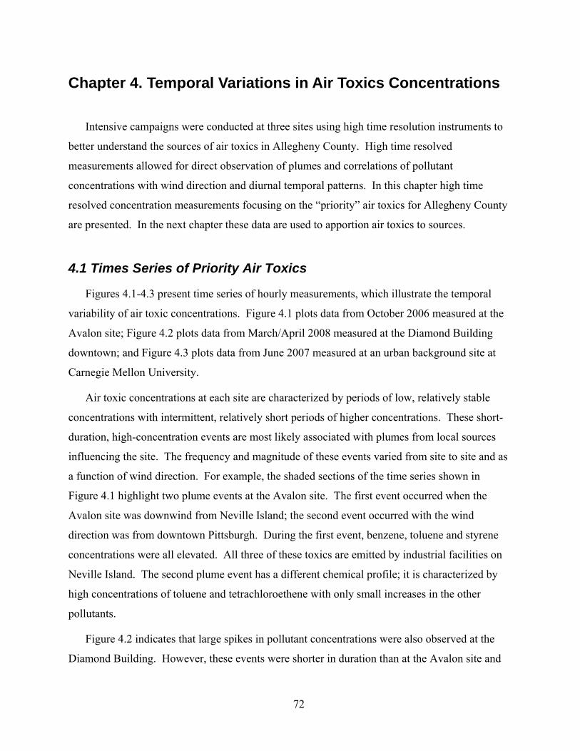
72
Chapter 4. Temporal Variations in Air Toxics Concentrations
Intensive campaigns were conducted at three sites using high time resolution instruments to
better understand the sources of air toxics in Allegheny County. High time resolved
measurements allowed for direct observation of plumes and correlations of pollutant
concentrations with wind direction and diurnal temporal patterns. In this chapter high time
resolved concentration measurements focusing on the “priority” air toxics for Allegheny County
are presented. In the next chapter these data are used to apportion air toxics to sources.
4.1 Times Series of Priority Air Toxics
Figures 4.1-4.3 present time series of hourly measurements, which illustrate the temporal
variability of air toxic concentrations. Figure 4.1 plots data from October 2006 measured at the
Avalon site; Figure 4.2 plots data from March/April 2008 measured at the Diamond Building
downtown; and Figure 4.3 plots data from June 2007 measured at an urban background site at
Carnegie Mellon University.
Air toxic concentrations at each site are characterized by periods of low, relatively stable
concentrations with intermittent, relatively short periods of higher concentrations. These short-
duration, high-concentration events are most likely associated with plumes from local sources
influencing the site. The frequency and magnitude of these events varied from site to site and as
a function of wind direction. For example, the shaded sections of the time series shown in
Figure 4.1 highlight two plume events at the Avalon site. The first event occurred when the
Avalon site was downwind from Neville Island; the second event occurred with the wind
direction was from downtown Pittsburgh. During the first event, benzene, toluene and styrene
concentrations were all elevated. All three of these toxics are emitted by industrial facilities on
Neville Island. The second plume event has a different chemical profile; it is characterized by
high concentrations of toluene and tetrachloroethene with only small increases in the other
pollutants.
Figure 4.2 indicates that large spikes in pollutant concentrations were also observed at the
Diamond Building. However, these events were shorter in duration than at the Avalon site and

73
the chemical profile of the plumes did not vary as much from event to event. Toluene and black
carbon concentrations were frequently elevated during plume events at the Diamond Building;
both of these species are associated with motor vehicle emissions. Tetrachloroethene
concentrations at Diamond Building were also highly variable; tetrachlorethene is used by dry
cleaners.
At the Carnegie Mellon University campus site, spikes in air toxic concentrations occurred
relatively infrequently (Figure 4.3). When they did occur they were relatively short, lasting an
hour or two. For the most part, concentrations were low and stable at the urban background site.
Although the time series shown in Figures 4.1 to 4.3 highlight the temporal variability in air
toxic concentrations, they provide little insight into underlying causes of this variability. What
fraction of the variability is driven by changes in wind direction? Are air toxics concentrations
always higher during certain times of the day or during certain days of the week? The high time
resolved data provide a unique opportunity to address these questions, which in turn provides
substantial insight into sources. These questions are the focus of the next two sections.
0
5
10
15
20
25
1-Oct 8-Oct 10-Oct 16-Oct 19-Oct 21-Oct
co
nc
en
tra
tio
n(
g/m
3 )
benzene
toluene
styrene
0
2
4
6
8
10
1-Oct 8-Oct 10-Oct 16-Oct 19-Oct 21-Oct
co
nc
en
tra
tio
n(
g/m
3 )
chloroform
ethylbenzene
tetrachloroethene
Figure 4.1 Time series of hourly concentrations measured during October 2006 at the Avalon site. The shaded regions indicate two of the many plumes that influenced this site.

74
0
2
4
6
8
20-Mar 22-Mar 24-Mar 26-Mar 28-Mar 30-Mar 1-Apr 3-Apr 5-Apr
Co
nc
en
tra
tio
n (
g/m
3 )
chloroform
ethylbenzene
tetrachloroethene
0
2
4
6
8
20-Mar 22-Mar 24-Mar 26-Mar 28-Mar 30-Mar 1-Apr 3-Apr 5-Apr
Co
nc
en
tra
tio
n (
g/m
3 o
r n
g/m
3 )
Black carbon (ug/m3)
Norhopane (ng/m3)
Pyrene (ng/m3)
0
2
4
6
8
10
12
20-Mar 22-Mar 24-Mar 26-Mar 28-Mar 30-Mar 1-Apr 3-Apr 5-Apr
Co
nce
ntr
atio
n (g
/m3 )
benzene
toluene
styrene
Figure 4.2 Time series of hourly air toxic concentrations measured during March-April 2008 at the downtown Diamond Building site.

75
0
1
2
3
4
5
6
7
6-Jun 11-Jun 15-Jun 20-Jun 22-Jun 26-Jun
co
nc
en
tra
tio
n (
g/m
3)
benzene
toluene
styrene
0
0.2
0.4
0.6
0.8
1
1.2
6-Jun 11-Jun 15-Jun 20-Jun 22-Jun 26-Jun
co
nc
en
tra
tio
n (
g/m
3)
chloroform
ethylbenzene
tetrachloroethene
Figure 4.3 Time series of hourly air toxic concentrations measured during June 2007 at Carnegie Mellon University.
4.2 The Effect of Wind Direction on Air Toxics Concentrations
Correlations of air toxic concentrations with wind direction can provide substantial insight
into the location of source regions. At Avalon a MET station was co-located with the high time
resolved instrument that measured wind speed and direction every minute. There was no MET
station at the downtown and urban background sites. To help interpret the air toxic data from
these sites, we used wind speed and direction measurements from the Hammerfield site located
on Tasso Street in Hazelwood.
Figure 4.4 shows wind roses for the Avalon and Hammerfield sites during the intensive
periods. The Avalon data are from September 2006-Febuary 2007. The Hammefield data are
from June 2007-February 2008. During the Avalon intensive, the wind came most frequently
from the west or Neville Island region. During the other intensives, the wind came most
frequently from the southwest and southeast.

76
Figure 4.4 Wind roses for the two meteorological stations, Avalon and Hammerfield.
Pollutant dispersion depends on a variety of meteorological factors in addition to wind
direction -- simply being downwind of a source is not sufficient to be strongly impacted by the
plume. Therefore, air toxic concentrations were binned by wind direction and then averaged.
Figure 4.5 plots the average concentrations of 7 priority air toxics and carbon disulfide as a
function of wind direction.

77
(Figure 4.5 cont. on next page)

78
Figure 4.5 Average air toxic concentrations (g/m3) as a function of wind direction for high time resolved measurements downtown, at the urban background site, and at the Avalon site. Averages calculated by binning data based on wind direction, as discussed in the text.
Figure 4.5 indicates that the concentrations of many air toxics exhibited strong wind
directional dependencies at all three sites. To help interpret these correlations, Figure 4.6

79
presents maps of Allegheny County showing the location of the monitoring sites used by this
project and major point sources. Allegheny County is the home to significant industry; there are
187 large point sources (>25 tons per year) that are required to report emissions to the Allegheny
County Health Department (1). As discussed below, emissions from two heavily industrialized
areas, the Neville Island area and the Clairton area, contributed significantly to gas-phase air
toxic concentrations at all three intensive sites.
Figure 4.7 shows a map of the Neville Island Area. It is highly industrialized with multiple
chemical manufacturing facilities and the Shenango Coke Works facility. The Allegheny
County Sanitary Authority (ACSA), a large source of chlorinated compounds, and the Valspar
Corporation, a large source of methyl isobutyl ketone (MIBK), are both located about one mile
up the Ohio River from Neville Island. There are large residential communities adjacent to the
Neville Island area, including the Stowe and Avalon neighborhoods.
Figure 4.8 shows a map of the sources in the heavy industrial area along the Monongahela
River. Of particular note is the Clairton area with three facilities that are among the largest
emitters of air toxics in the county: USS Clairton Coke Works, Hercules Inc., and the Eastman
Chemical Resins Inc. For example, the combined emissions of these three sources are 207 TYP
of toluene (71% of total large point source toluene emissions in Allegheny County) and 87 TPY
of Benzene (84% of total large point source benzene emissions).

80
Figure 4.6 Map of Allegheny County with the two industrial areas affecting air toxics concentrations outlined. a) Neville Island area and b) up river industrial area

81
Figure 4.7 Map of the Neville Island area shown in section (a) from Figure 4.6
Figure 4.8 Map of the upriver industrial area shown as section (b) in Figure 4.6.
Figure 4.5 indicates that Neville Island is a major source of air toxics in Avalon. For
example, the concentrations of benzene and carbon disulfide were, on average, much higher
when the site was downwind of Neville Island. All of these toxics are emitted by industrial
facilities on the island. However, the industrial facilities on Neville Island are not the only
important local sources of air toxics in Avalon. For example, the concentrations of chloroform,

82
tetrachloroethene, toluene and trichloroethene were all elevated when Avalon was downwind of
downtown Pittsburgh (i.e., when the wind was blowing down the Ohio River).
The wind directional dependence of selected air toxics measured at the Diamond Building in
downtown Pittsburgh are also shown in Figure 4.5. Concentrations of benzene, toluene, and
carbon disulfide at the Diamond Building are higher when the wind is blowing from either the
Neville or Clairton source regions. Other compounds are only elevated when the wind is
blowing in one of these two directions. For example, ethylbenzene concentrations are elevated
when the wind is blowing down the Monongahela River. Styrene and to a lesser extent
trichloroethene concentrations are often elevated when the wind is blowing from Neville Island
but not from the Clairton industrial area. There are several large sources of styrene on Neville
Island.
The wind directional dependence of air toxics measured at Carnegie Mellon University is
shown in Figure 2.5. For example, concentrations of many toxics are higher when the wind is
blowing from the Clairton area. Neville Island does not appear to have an effect on
concentrations at CMU.
Concentrations of some air toxics did not exhibit strong wind directional dependencies. For
example pollutants with few sources and thought to be regionally distributed, such as carbon
tetrachloride, bromoform, and 1,2-dichloroethane, did not show any wind directional dependence
and pollutants with a large number of small emitting sources such as chloroform.
4.3 Temporal Patterns in Air Toxics Concentrations
Temporal patterns of air toxic concentrations provide information on sources and acute
exposures. Day of the week and hour of the day patterns were investigated using the high time
resolved data. Seasonal patterns were investigated with the baseline data. High time resolved
data were used to determine diurnal, weekly, and wind directional patterns for air toxics
concentrations. The data were binned by hour of the day or day of the week and the bootstrap
method (11) was used to determine confidence intervals on the mean.

83
4.3.1 Day of the Week Patterns in Air Toxics Concentrations
Figure 4.9 plots average weekend and weekday concentrations of selected air toxics. There
were statistically significant differences between weekday and weekend concentrations, but not
between individual week days (e.g., Monday versus Tuesday) or between weekend days
(Saturday versus Sunday). The weekend/weekday patterns indicate the importance of local
sources whose emissions are higher during the work week.
Many air toxics at the Diamond Building have a strong weekday/weekday pattern, with lower
concentrations observed on weekends. For example, concentrations of mobile source air toxics
such as toluene, benzene, and ethylbenzene concentrations are about 50% higher on weekdays
then weekends. Weekday concentrations of condensed phase markers of motor vehicle
emissions (BC, hopanes, steranes) were about a factor of two higher than weekend
concentrations. Other, non-mobile source air toxics, such as tetrachloroethene, also follow a
distinctive weekend/weekday pattern. These patterns mirror the economic activity downtown.
The relatively large variation in concentrations of BC and other mobile tracers relative to
benzene may imply that the gas phase species have more sources.
Many air toxics also have statistically significant weekday/weekend variation at the Carnegie
Mellon University campus (the site of the background intensive). Therefore, local sources with
emissions during the normal work week are important at this site. However, Figure 4.9 indicates
that there were no clear weekend/weekday patterns in the Avalon air toxics concentrations. This
underscores the large contribution that emissions from industrial facilities that operate seven
days a week make to the Avalon site.

84
0
0.5
1
1.5
2
2.5
3
benzene toluene tetra-chloroethene
ethyl-benzene
DO
WN
TO
WN
co
nc
en
tra
tio
n (
g/m
3 ) weekday
weekend
0
0.05
0.1
0.15
0.2
0.25
carbondisulfide
chloroform trichloro-ethene
styrene
weekday
weekend
0
1
2
3
4
5
6
benzene toluene tetra-chloroethene
ethyl-benzene
AV
AL
ON
co
nc
en
tra
tio
n (
g/m
3 )
weekday
weekend
0
0.2
0.4
0.6
0.8
1
1.2
carbondisulfide
chloroform trichloro-ethene
styrene
weekday
weekend
0
0.5
1
1.5
benzene toluene tetra-chloroethene
ethyl-benzene
BA
CK
GR
OU
ND
co
nc
en
tra
tio
n (
g/m
3 )
weekday
weekend
0
0.1
0.2
0.3
0.4
carbondisulfide
chloroform trichloro-ethene
styrene
weekday
weekend
0
0.5
1
1.5
2
2.5
3
BlackCarbon
Norhopane hopane
weekday
weekend
Figure 4.9 Average weekday and weekend concentrations of air toxics measured during the intensive campaigns. The error bars indicate the 5th and 95th percentile confidence interval of the mean using the bootstrap method.
4.3.2 Diurnal Patterns of Air Toxics Concentrations
Average diurnal patterns for eight air toxics are shown in Figure 4.10. Except for a few
compounds, air toxic concentrations were lower during the day than at night. This reflects the
strong influence that mixing or boundary layer height has on pollutant concentrations. During
the night the boundary layer is low, which traps local emissions and creates higher pollutant
concentrations. During the day, the boundary layer rises, reducing pollutant concentrations.
Minimum concentrations often occurred around noon when the boundary layer is highest.
The magnitude of the diurnal pattern reflects the strength of local sources. At one extreme is
carbon tetrachloride which exhibits no diurnal pattern (Figure 4.10). Carbon tetrachloride is a
chlorofluorocarbon with a long atmospheric lifetime. Its emissions were substantially reduced
by the Montreal Protocol. The net result of these two factors is that carbon tetrachloride is more

85
or less homogeneously distributed throughout the atmosphere. Therefore, diurnal variations in
the mixing layer height do not affect local concentrations. At the other extreme is styrene
concentration at the Avalon site (Figure 4.10). The chemical facilities on Neville Island are large
sources of styrene, and changes in boundary layer height causes the styrene concentrations to
vary by more than a factor of three over the course of the day.
Daily cycles in emissions can also contribute to diurnal patterns in air toxic concentrations.
At the downtown site, concentrations of air toxics associated with mobile source emissions begin
increasing around four in the morning, reaching a peak around seven in the morning. The
ethylbenzene concentrations plotted in Figure 4.10 provide the clearest example of this pattern.
It is caused by the combined effects of varying emissions and varying boundary layer height.
Motor vehicle use begins increasing in the very early in the morning, but the peak air toxic
concentrations do not correspond to the peak in traffic volume because of the strong influence of
boundary layer height on pollutant concentrations. A much weaker peak can also be observed in
the afternoon for benzene, toluene, and ethylbenzene. This peak is presumably caused by the
evening rush hour. It is much smaller than the morning peak because of the large difference in
boundary layer height. Another factor may be evening rush hour may be spread out over a
longer period of time than the morning rush, essentially dispersing the emissions in time.
Concentrations of several chlorinated air toxics also exhibit distinctive diurnal patterns. For
example, tetrachloroethene concentrations at the Diamond Building have a unique diurnal
pattern. There is a spike in the early morning mirroring the spike in mobile source air toxics
concentrations and a second peak between around 10 AM and 2 PM. Tetrachloroethene is used
as a solvent by dry cleaners; mobile sources are not a source of chlorinated air toxics.
At the Avalon site, the mixing layer height has a strong effect on concentrations of
chloroform, ethylbenzene and toluene but not on benzene. Local emissions of benzene appear to
increase concentrations during midday.

86
Avalon Downtown Urban Background
Benzene
CarbonTetrachloride
Tetrachloro-ethene
Trichloro-ethene
Toluene
Styrene
Ethyl-benzene
Chloroform
01234567
Co
nc
en
tra
tio
n (g
/m3 )
0
0.5
1
1.5
2
2.5
0
0.2
0.4
0.6
0.8
1
1.2
0
0.1
0.2
0.3
0.4
0.5
0.6C
on
ce
ntr
atio
n (g
/m3 )
0
0.1
0.2
0.3
0.4
0.5
0.6
0
0.1
0.2
0.3
0.4
0.5
0.6
0
0.5
1
1.5
2
Co
nce
ntr
atio
n (g
/m3 )
0
1
2
3
4
0
0.1
0.2
0.3
0.4
0
0.1
0.2
0.3
Co
nc
entr
atio
n (g
/m3)
0
0.1
0.2
0.3
0
0.1
0.2
0.3
0
1
2
3
4
5
6
7
Co
nce
ntr
atio
n (g
/m3)
0
1
2
3
4
0
0.5
1
1.5
2
0
0.5
1
1.5
2
2.5
Co
nce
ntr
atio
n (g
/m3)
0
0.1
0.2
0.3
00.10.20.30.40.50.60.70.8
0
0.2
0.4
0.6
0.8
1
Co
nce
ntr
atio
n (g
/m3)
0
0.5
1
1.5
2
0
0.05
0.1
0.15
0.2
0.25
0.3
0.35
0
0.1
0.2
0.3
0:004:00
8:0012:00
16:00
20:00Time of Day
Co
nce
ntr
atio
n (g
/m3)
0
0.02
0.04
0.06
0.08
0.1
0.12
0.14
0:004:00
8:0012:00
16:00
20:00Time of Day
0
0.04
0.08
0.12
0.16
0.2
0:004:00
8:0012:00
16:00
20:00Time of Day
Figure 4.10 Average diurnal profiles of air toxic concentrations at the three intensive sites. Symbols indicate the mean concentration at each hour and error bars represent 95th percentile confidence interval on the mean. Note that concentration scale changes between sites.

87
The magnitude of the diurnal variations at the Carnegie Mellon University site was
significantly smaller compared to those in Avalon or downtown. For example, only minor
diurnal patterns can be seen for mobile compounds. This underscores that emissions from very
local sources are a large contributor to air toxic concentrations at the Carnegie Mellon University
site.
0
0.5
1
1.5
2
2.5
3
3.5
0 4 8 12 16 20Time of Day
Black Carbon
00.10.20.30.40.50.60.70.80.9
0 4 8 12 16 20Time of Day
Hopane
00.10.20.30.40.50.60.70.80.9
0 4 8 12 16 20Time of Day
Co
nc
en
tra
tio
n (
g/m
3 ) Norhopane
Figure 4.11 Average diurnal profiles of condensed phase compounds associated with motor vehicle emissions measured at the Diamond Building. Symbols represent the mean concentration and error bars represent the standard error of the mean. Note that concentration scale changes between sites.
4.3.3 Seasonal Patterns of Air Toxics Concentrations
We analyzed the baseline data for seasonal patterns in air toxic concentrations. Figure 4.12
plots seasonal average concentrations for a few air toxics with interesting seasonal patterns.
Concentrations of most toxics did not exhibit a statistically significant seasonal pattern.
Seasonal patterns (or the lack thereof) provide insight into the sources of air toxics that are
both directly emitted by sources and photochemically produced in the atmosphere.
Formaldehyde and acetaldehyde are examples of two toxics with primary and secondary sources.
Figure 4.12 indicates that formaldehyde concentrations were substantially higher during the
summer than during other seasons at all four baseline sites. There is a significant increase in
photochemical production in the summer. Therefore, atmospheric oxidation of volatile organic
compounds is an important source of formaldehyde in Allegheny County. In contrast,
acetaldehyde does not exhibit any seasonal pattern; therefore primary emissions (presumably
motor vehicles) are the dominant source of acetaldehyde in Allegheny County.
Figure 4.12 indicates that propionaldehyde concentrations also exhibited a distinctive
seasonal pattern. Propionaldehyde concentrations were about a factor of two higher at the four
baseline sites in the fall than during other seasons. Biomass burning is one source of

88
propionaldehyde. Previous research has shown the highest levels of biomass smoke in
Allegheny County occur in the fall (23).
0
1
2
3
4
Fall Spring Summer Winter
co
nc
entr
atio
n (
g/m
3)
Formaldehyde
0
1
2
3
4
Fall Spring Summer Winter
con
cen
trat
ion
(
g/m
3)
Acetaldehyde
0
0.2
0.4
0.6
0.8
1
1.2
1.4
1.6
Fall Spring Summer Winter
con
cen
tra
tio
n (
g/m
3)
Propionaldehyde
Figure 4.12 Seasonal patterns of selected air toxics measured during the baseline study.
4.4 Chlorinated Compounds
Several chlorinated air toxics posed large cancer risks downtown, but not at the other
baseline sites. Many of these chlorinated compounds are commonly used as solvents, but this
project has not been able to define the emission sources of many of these toxics. This section
presents data on temporal and wind direction patterns for selected chlorinated toxics in the
downtown area.

89
Trichloroethene: Trichloroethene is estimated to pose a lifetime cancer risk of 2 x 10⁻⁵ at the
Flag site, which is about a factor of twenty higher than cancer risk it poses at any other site.
Figure 4.13 shows a time series of trichloroethene measured at the Flag Plaza site over a ten year
period. Trichloroethene concentrations at this site are highly variability, with most of the
exposure being driven by short periods of days or months with relatively elevated concentrations.
High concentrations of trichloroethene were not observed during the intensive study at the
Diamond Building which is about 1/2 km from Flag Plaza. However, Figure 4.13 indicates
trichloroethene concentrations were also low at Flag Plaza during this study (first six months of
2008). Therefore, the spatial extent of the trichloroethene hotspot in the downtown area is not
well understood. It could be extremely localized around the Flag Plaza area or it could affect the
larger downtown area.
0
1
2
3
4
5
6
7
1997 1998 1999 2000 2001 2002 2003 2004 2005 2006 2007 2008
co
nc
en
tra
tio
n (
g/m
3 )
Figure 4.13 Quarterly average concentrations of trichloroethene measured at the Flag Plaza site from 1997 to the second quarter of 2008.
1,4-Dichlorobenzene: 1,4-dichlorobenzene is another chlorinated toxic that posed
substantially higher risks downtown than at the other baseline sites. Of the 36 target organic air
toxics, 1,4-dichlorobenzene poses 9% of the cancer risks downtown versus 1-2% of the risks at
the background and industrial influence sites (Avalon and Stowe). Elevated concentrations of
1,4-dichlorobenzene were also observed during the intensive study at the Diamond Building
indicating that the problem is not localized to the Flag Plaza site.
The intensive data at the Diamond Building indicate that 1,4-dichlorobenzene concentrations
downtown have distinctive temporal and wind directional patterns. Figure 4.14 indicates that
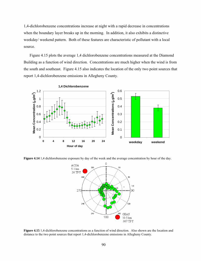
90
1,4-dichlorobenzene concentrations increase at night with a rapid decrease in concentrations
when the boundary layer breaks up in the morning. In addition, it also exhibits a distinctive
weekday/ weekend pattern. Both of these features are characteristic of pollutant with a local
source.
Figure 4.15 plots the average 1,4 dichlorobenzene concentrations measured at the Diamond
Building as a function of wind direction. Concentrations are much higher when the wind is from
the south and southeast. Figure 4.15 also indicates the location of the only two point sources that
report 1,4-dichlorobenzene emissions in Allegheny County.
0
0.1
0.2
0.3
0.4
0.5
0.6
weekday weekend
Me
an
Co
nc
en
tra
tio
ns
(
g/m
3 )
1,4 Dichlorobenzene
0
0.2
0.4
0.6
0.8
1
1.2
0 4 8 12 16 20 24
Hour of day
Me
an
Co
nc
en
tra
tio
n (
g/m
3 )
Figure 4.14 1,4 dichlorobenzene exposure by day of the week and the average concentration by hour of the day.
Figure 4.15 1,4-dichlorobenzene concentrations as a function of wind direction. Also shown are the location and distance to the two point sources that report 1,4-dichlorobenzene emissions in Allegheny County.

91
Methylene chloride: Although methylene chloride risks in Allegheny County are low,
methylene chloride concentrations downtown are comparable to the national 75th percentile.
Figure 4.16 indicates that these high concentrations are associated with a source located to the
south or east of the Diamond Building. Methylene chloride also has a distinctive weekend/
weekday pattern.
Figure 4.16 On the left is the average concentration of methylene chloride as a function of wind direction. On the right is the average concentration during the week and weekend. The error bars indicate the 95th percentile confidence intervals of the mean.

92
Chapter 5. Receptor Modeling of Air Toxic Concentrations and Risks
One of the main goals of this project was to identify the sources of priority air toxics in
Allegheny County. The high time resolved measurements from the intensive studies are ideally
suited for source apportionment because they resolve plume events helping to pinpoint source
locations. In this chapter a receptor model was used to apportion 27 air toxics and 13 volatile
organic compounds (VOCs) to sources.
5.1 Cancer Risk from Baseline and Intensive Studies
Before presenting the source apportionment results we compare the cancer risks estimated
from the baseline and intensive datasets. This comparison is important because the source
apportionment modeling was performed on the high time resolved data collected during the
intensive studies. These data were collected over a much shorter period and therefore may not
accurately represent chronic risks.
Figure 5.1 compares the risk profiles from the intensive and baseline studies for the subset of
the compounds included in the source apportionment model. There is excellent agreement
between the two risk profiles for the Avalon site. Therefore the intensive sampling was long
enough to accurately characterize chronic risks at this site.
Figure 5.1 indicates that there is only reasonable agreement between the risk profiles derived
from the other two sets of data. This is not surprising since the intensive and baseline studies
conducted to characterize background and downtown air toxic concentrations were not made at
the same sites. The background intensive site was located at Carnegie Mellon University, 13.4
miles away from the baseline background site, South Fayette. The downtown intensive site was
located in the Diamond Building, 1.2 km away from the Flag Plaza site used for the baseline
study.
The main differences between the risk profiles at the two downtown sites are associated with
chlorinated air toxics. The cancer risks associated with trichloroethene are much lower and the
cancer risk associated with tetrachloroethene is much higher at the Diamond Building compared
to Flag Plaza. The major differences between the risk profiles at the two background sites are
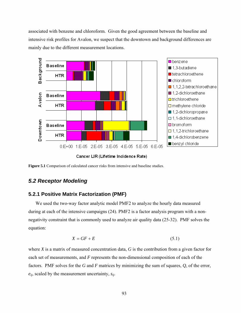
93
associated with benzene and chloroform. Given the good agreement between the baseline and
intensive risk profiles for Avalon, we suspect that the downtown and background differences are
mainly due to the different measurement locations.
Figure 5.1 Comparison of calculated cancer risks from intensive and baseline studies.
5.2 Receptor Modeling
5.2.1 Positive Matrix Factorization (PMF)
We used the two-way factor analytic model PMF2 to analyze the hourly data measured
during at each of the intensive campaigns (24). PMF2 is a factor analysis program with a non-
negativity constraint that is commonly used to analyze air quality data (25-32). PMF solves the
equation:
EGFX (5.1)
where X is a matrix of measured concentration data, G is the contribution from a given factor for
each set of measurements, and F represents the non-dimensional composition of each of the
factors. PMF solves for the G and F matrices by minimizing the sum of squares, Q, of the error,
eij, scaled by the measurement uncertainty, sij.

94
2)/( ifij seQ (5.2)
Two important user inputs for PMF analysis are the number of factors and the degree of
matrix rotation. These parameters were systematically varied and a number of diagnostic tools
were used to select the optimum solution.
Interpretability was the key basis for judging the optimum values for the number of factors
and degree of matrix rotation. Interpretability was assessed by examining factor contributions as
a function of wind direction and comparing factor profiles with actual source profiles. For
example, factor contributions that are strongly correlated with wind direction can point directly
to the source of the emissions. Weekend/weekday patterns can help identify whether the factor
is associated with an industrial or mobile source. Factor profiles were compared to source
profiles from the ACHD point source emission inventory (1), the EPA Mobile Source Air Toxics
website (5) and the literature(33-38). We also considered several measures of statistical quality
of the fit including included plotting the maximum individual column mean of the residual
matrix, IM, as a function of the maximum individual column standard deviation, IS; examining
the largest element in the rotmax matrix; miminizing the Q value, and G-space mapping (39).
However multiple solutions satisfied these statistical tests.
5.2.2 Pollutants Apportioned Using PMF
Table 5.1 lists the compounds included in the PMF analysis. Separate analyses were
performed for each intensive site, and slightly different sets of pollutants were included in the
PMF models for each site.
PMF identifies factors based on varying pollutant concentrations. Therefore, only air toxics
with significant spatial and/or temporal concentration variations were included in the model.
Although this represents only a subset of the air toxics measured by this study, toxics with time
varying concentrations are the ones strongly influenced by emissions from local sources. The
sources of other air toxics not included in the PMF model are discussed in Chapter 8.
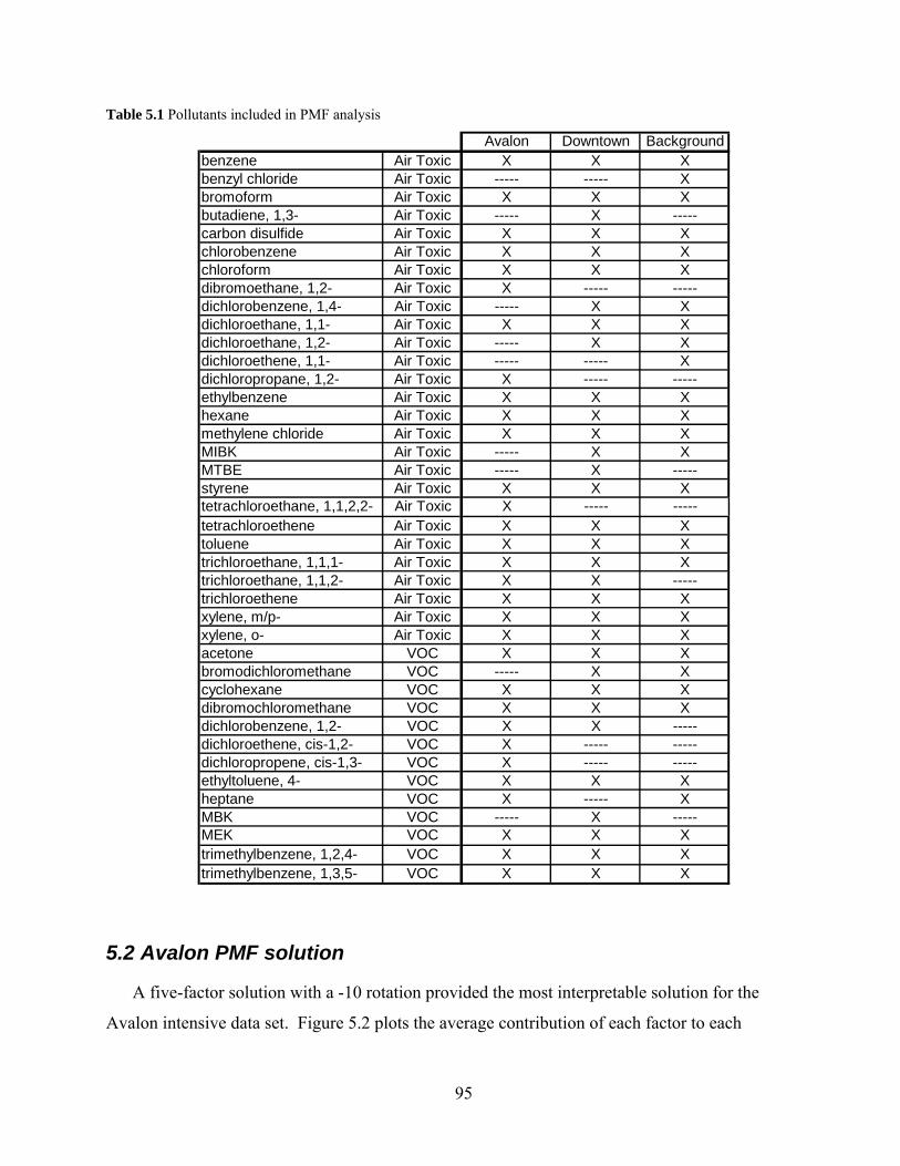
95
Table 5.1 Pollutants included in PMF analysis
Avalon Downtown Backgroundbenzene Air Toxic X X Xbenzyl chloride Air Toxic ----- ----- Xbromoform Air Toxic X X Xbutadiene, 1,3- Air Toxic ----- X -----carbon disulfide Air Toxic X X Xchlorobenzene Air Toxic X X Xchloroform Air Toxic X X Xdibromoethane, 1,2- Air Toxic X ----- -----dichlorobenzene, 1,4- Air Toxic ----- X Xdichloroethane, 1,1- Air Toxic X X Xdichloroethane, 1,2- Air Toxic ----- X Xdichloroethene, 1,1- Air Toxic ----- ----- Xdichloropropane, 1,2- Air Toxic X ----- -----ethylbenzene Air Toxic X X Xhexane Air Toxic X X Xmethylene chloride Air Toxic X X XMIBK Air Toxic ----- X XMTBE Air Toxic ----- X -----styrene Air Toxic X X Xtetrachloroethane, 1,1,2,2- Air Toxic X ----- -----tetrachloroethene Air Toxic X X Xtoluene Air Toxic X X Xtrichloroethane, 1,1,1- Air Toxic X X Xtrichloroethane, 1,1,2- Air Toxic X X -----trichloroethene Air Toxic X X Xxylene, m/p- Air Toxic X X Xxylene, o- Air Toxic X X Xacetone VOC X X Xbromodichloromethane VOC ----- X Xcyclohexane VOC X X Xdibromochloromethane VOC X X Xdichlorobenzene, 1,2- VOC X X -----dichloroethene, cis-1,2- VOC X ----- -----dichloropropene, cis-1,3- VOC X ----- -----ethyltoluene, 4- VOC X X Xheptane VOC X ----- XMBK VOC ----- X -----MEK VOC X X Xtrimethylbenzene, 1,2,4- VOC X X Xtrimethylbenzene, 1,3,5- VOC X X X
5.2 Avalon PMF solution
A five-factor solution with a -10 rotation provided the most interpretable solution for the
Avalon intensive data set. Figure 5.2 plots the average contribution of each factor to each

96
species. Figure 5.3 shows the apportionment of the additive cancer risk for the air toxics
included in the PMF model to the five factors; two of the factors contribute more than 75% of the
cancer risks.
1.00.80.60.40.20.0Fractional Factor Contribution to Outdoor Concentrations
styrene
acetonemethyl ethyl ketone
bromoformchlorobenzene
dichlorobenzene, 1,2-
dibromochloromethanedichloroethane, 1,1-
trimethylbenzene, 1,3,5-xylene, m/p-
dichloropropene, cis-1,3-ethylbenzene
xylene, o-hexane
trichloroethane, 1,1,2-toluene
ethyltoluene, 4-trimethylbenzene, 1,2,4-
tetrachloroethenecyclohexane
tetrachloroethane, 1,1,2,2-dibromoethane, 1,2-
dichloroethene, cis-1,2-trichloroethane, 1,1,1-dichloropropane, 1,2-
trichloroethenemethylene chloride
chloroform
benzenecarbon disulfide
Neville Island Styrene Factor Dominated
Secondary/Background Factor Dominated
Downtown Factor Dominated
ACSA Factor Dominated
Neville Island Benzene Factor Dominated
Neville Island Styrene Factor Secondary/Background FactorDowntown Factor ACSA FactorNevile Island Benzene Factor
Figure 5.2 Factor contributions to air toxic concentrations at the Avalon site.

97
8%4%
30%
12%
46%
Neville Island Styrene Factor
Seconday/ Background Factor
Downtown Factor
ACSA Factor
Neville Island Benzene Factor
Figure 5.3 Apportionment of cancer risk for the Avalon site.
Neville Island Benzene Factor: One factor contributed 66% of the benzene and nearly half
of the risks at Avalon site. Two pieces of evidence strongly link this factor with emissions from
Shenango Coke Works on Neville Island. First, Figure 5.4 shows that the contribution of this
factor is extremely wind directionally dependent with its contributions being significantly
elevated when wind is coming from the Shenango Coke Works on Neville Island, a large source
of benzene (1). Second, Figure 5.6 indicates excellent agreement between the benzene factor
profile and the Shenango source profile. Finally, Figure 5.5 indicates that there is no
weekend/weekday pattern in the contribution of this factor, consistent with an industrial source
that operates all of the time. Therefore, this factor appears associated with emissions from
industrial sources on Neville Island, specifically the Shenango Coke Works.

98
Figure 5.4 Mean contribution for Benzene factor as a function of wind direction.
Benzene Factor
0
1
2
3
4
5
6
7
8
0 4 8 12 16 20 24
Hour of day
Me
an
Co
nc
en
tra
tio
n (
g/m
3 )
0
0.5
1
1.5
2
2.5
3
3.5
Weekday Weekend
Me
an
Co
nc
en
tra
tio
ns
(
g/m
3 )
Figure 5.5 Diurnal patterns of factor contribution and factor contribution as a function of day of the week for the Benzene factor.

99
0.0
0.1
0.2
0.3
0.4
0.5
0.6
0.7
0.8
0.9
1.0
SHENANGOINC.
USS -CLAIRTON
WORKS
BenzeneFactor
Fra
cti
on
al C
on
trib
uti
on 1,1,2,2-tetrachloroethane
1,2,4-Trimethylbenzene
Hexane
carbon disulfide
ethylbenzene
styrene
toluene
benzene
Figure 5.6 Comparison of the Neville Island Benzene Factor to emission profiles for two coke works in Allegheny County. Shenango is located on Neville Island near Avalon and Clairton is the largest coke works in Allegheny County.
Downtown Factor: The downtown factor is the second largest contributor to risks in
Avalon. This factor was named the downtown factor because its contribution was elevated when
the wind was coming from the east, the direction of downtown Pittsburgh (Figure 5.7). The
downtown factor contributes 53%, 60%, and 25% of toluene, xylenes and benzene in Avalon,
respectively. All of these compounds are emitted by mobile sources.
Figure 5.8 compares the species distribution in the downtown factor to gasoline and diesel
vehicle source profiles. The downtown factor profile agrees well with the gasoline vehicle
source profile. Therefore, we associated this factor with gasoline vehicle emissions. However,
emissions of non-mobile source air toxics were also apportioned to this factor. For example, the
chlorinated compounds in this factor are from non-mobile sources in the downtown area. These
chlorinated toxics are likely from sources in downtown Pittsburgh that are co-varying with the
mobile source emissions. Sixty percent of the risks apportioned to the downtown factor come
from mobile source air toxics and 40% come from chlorinated compounds.

100
Figure 5.7 Mean factor contribution of the downtown factor in Avalon as a function of wind direction.
0.0
0.2
0.4
0.6
0.8
1.0
MediumDiesel
GasolineCatalyst
Equipted
Downtownfactor
Fra
cti
on
al C
on
trib
uti
on
benzene toluene ethylbenzenem/p-xylene o-xylene carbon disulfidehexane 1,2,4-trimethylbenzene cyclohexaneacetone styrene chlorinated compoundsother
Figure 5.8 Comparison of the downtown factor to mobile source profiles (33, 34).
ACSA Factor: PMF apportioned 56% of the trichloroethene and 46% of the
tetrachloroethene measured in Avalon to one factor. Two pieces of evidence strongly link this

101
factor to emissions from the Allegheny County Sanitary Authority (ACSA). First, Figure 5.9
indicates that the factor profile closely matches the emissions profile from ACSA. Second, the
factor contribution has a strong wind directional dependence with highest concentrations being
associated with wind coming from the direction of ACSA, Figure 5.10. This factor contributes
12% of the additive cancer risk at the Avalon site.
0.0
0.2
0.4
0.6
0.8
1.0
Chlorinated Organics Factor Allegheny County SanitaryAuthority
Fra
cti
on
al C
on
trib
uti
on
toluene xylenes 1,2,4-trimethylbenzenetetrachloroethene ethylbenzene MEKcarbon disulfide methylene chloride 1,1-dichloroethanechloroform cyclohexane cis-1,2-dichloroetheneheptane 1,1,1-trichloroethane benzenetrichloroethene 1,2-dichloropropane cis-1,3-dichloropropene1,1,2-trichloroethane 1,2-dibromoethane bromoformchlorobenzene acetone styrene1,1,2,2-tetrachloroethane 4-ethyltoluene 1,3,5-trimethylbenzene1,2-dichlorobenzene hexane
Figure 5.9 Comparison of Allegheny County Sanitary Authority emissions profile and the profile of the ASCA PMF factor

102
Figure 5.10 Mean concentration of the ACSA as a function of wind direction.
Neville Island Styrene Factor: One factor contributed almost 80% of the styrene and 8% of
the cancer risk in Avalon. Figure 5.11 indicates that this factor contribution is higher when
Avalon is downwind of Neville Island or downtown Pittsburgh. The contribution of this factor
does not vary with day of the week (Figure 5.12) suggesting an industrial source. Its
contribution varies diurnally increasing overnight followed by a rapid decrease associated with
the break-up of the boundary layer in the morning.
Two large chemical companies are located on Neville Island, The Neville Chemical
Company and Ashland Specialty Chemical Co. Both facilities are major sources of styrene (1).
Figure 5.13 compares the factor profile of the Styrene factor to a composite source profile that is
an emissions weighted average profile of these two facilities (1). There is excellent agreement
with this factor and this composite source profile.

103
Figure 5.11 Mean contribution of styrene factor as a function of wind direction.
Styrene Factor
0
1
2
3
4
5
6
7
8
0 4 8 12 16 20 24
Hour of day
Me
an
Co
nc
en
tra
tio
n (
g/m
3 )
0
0.5
1
1.5
2
2.5
3
Weekday Weekend
Me
an
Co
nc
en
tra
tio
ns
(
g/m
3 )
Figure 5.12 Diurnal patterns of factor contribution and factor contribution as a function of day of the week for the Styrene factor.

104
Figure 5.13 Comparison of large styrene emitting point source profiles and the profile of the Styrene Factor.
Secondary/Background Factor: PMF attributed the majority of the methyl ethyl ketone and
acetone, two secondary components, to one factor. This factor shows no wind directional
dependence or diurnal pattern (Figures 5.14 and 5.15) consistent with secondary sources. This
factor is a minor contributor to risk.

105
2 4
6
30
210
60
240
90270
120
300
150
330
180
0
Figure 5.14 Mean concentration of secondary/background factor as a function of wind direction.
Figure 5.15 Diurnal patterns of factor contribution and factor contribution as a function of day of the week for the Secondary/Background Factor.
5.2.1 Discussion of Avalon PMF Results
The risk apportionment by PMF is summarized in Figure 5.16. First, the compounds
included in the PMF model only contributed 34% of additive cancer risk of the 36 target organic
air toxics. As previously discussed, only air toxics with significant temporal and/or spatial
variability were included in the PMF model. These toxics are the ones that are strongly
influenced by emissions from local sources. Chapter 8 synthesizes all of the risk estimates,
Secondary/Background Factor
0
1
2
3
4
5
6
7
8
9
0 4 8 12 16 20 24
Hour of day
Me
an
Co
nc
en
tra
tion
(
g/m
3 )
0
0.5
1
1.5
2
2.5
3
3.5
4
4.5
Weekday Weekend
Me
an
Co
nc
entr
ati
on
s (
g/m
3 )

106
quantifying the contribution of regional sources and other compounds not included in the PMF
model.
Of the compounds included in the Avalon PMF model, Figure 5.16 indicates that PMF
apportioned 55% of the additive cancer risk to emissions from sources on Neville Island. The
majority of this risk is associated with emissions from the Shenango Coke Works (Neville Island
benzene factor). Therefore, industrial facilities on Neville Island are not the only local sources
of air toxics in Avalon. Emissions from downtown Pittsburgh and ACSA contributed 30% and
12% of the additive cancer risk, respectively.
The PMF results also highlight potential discrepancies in the reported emissions from
industrial sites on Neville Island. According to the ACHD point source emissions inventory (1),
both Shenango and Neville Chemical Company emit similar quantities of benzene per year, 2.96
TPY and 3.64 TPY, respectively. However, PMF apportioned seven times more benzene to the
coke factor than the chemical company factor.
Figure 5.16 also shows that the PMF solution also provides insight into the relative
importance of emissions from mobile, non-mobile, and regional sources in Avalon. Three of the
factors are clearly associated with emissions from non-mobile or industrial sources: the two
Neville Island factors and the ACSA factor. However, the downtown factor is a mixture of
emissions from mobile and non-mobile sources. A reasonable assumption is to assign the risk
contributed by Mobile Source Air Toxics (MSATs) (benzene toluene, etc. (5, 33, 34))
apportioned to the downtown factor to mobile source emissions and to attribute any remaining
risk to non-mobile sources. This approach splits the risk apportioned to the downtown factor:
60% to mobile and 40% to non-mobile sources. Therefore, 79% of the cancer risk apportioned
by PMF in Avalon is due to mobile sources and only 17% of the risks to non-mobile sources.
Finally, Figure 5.16 indicates that the risks from non-mobile sources can be further broken done
into specific sources with coke works emissions dominating non-mobile source contribution.
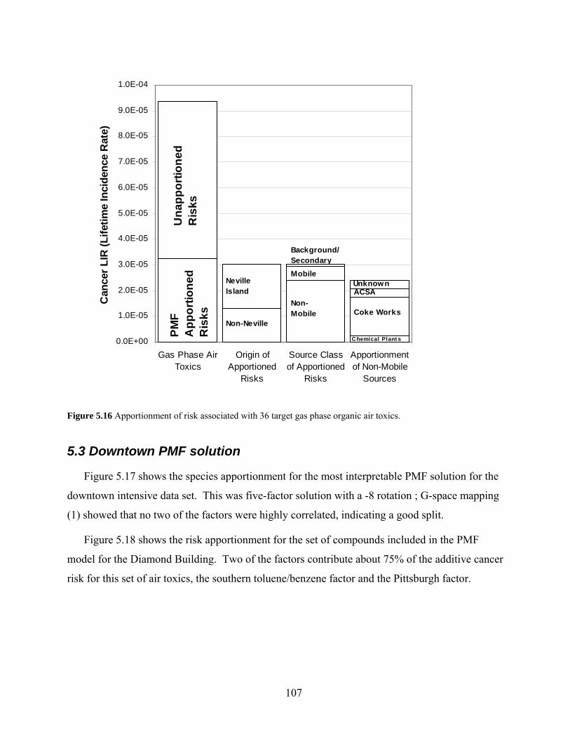
107
0.0E+00
1.0E-05
2.0E-05
3.0E-05
4.0E-05
5.0E-05
6.0E-05
7.0E-05
8.0E-05
9.0E-05
1.0E-04
Gas Phase AirToxics
Origin ofApportioned
Risks
Source Classof Apportioned
Risks
Apportionmentof Non-Mobile
Sources
Can
cer
LIR
(L
ifet
ime
Inci
den
ce R
ate)
Neville Island
Non-Neville
Background/ Secondary
Non-Mobile
MobileUnknown
Coke Works
C hemical Plant s
ACSA
Un
ap
po
rtio
ne
d
Ris
ks
PM
F
Ap
po
rtio
ne
d
Ris
ks
Figure 5.16 Apportionment of risk associated with 36 target gas phase organic air toxics.
5.3 Downtown PMF solution
Figure 5.17 shows the species apportionment for the most interpretable PMF solution for the
downtown intensive data set. This was five-factor solution with a -8 rotation ; G-space mapping
(1) showed that no two of the factors were highly correlated, indicating a good split.
Figure 5.18 shows the risk apportionment for the set of compounds included in the PMF
model for the Diamond Building. Two of the factors contribute about 75% of the additive cancer
risk for this set of air toxics, the southern toluene/benzene factor and the Pittsburgh factor.

108
1.00.80.60.40.20.0Fractional Factor Contribution to Outdoor Concentrations
benzyl chloridestyrenetoluene
carbon disulfideMIBK
ethyltoluene, 4-trichloroethene
trichloroethane, 1,1,2-
tetrachloroethene
MTBEbutadiene, 1,3-
dichlorobenzene, 1,2-bromoform
chlorobenzenehexane
trimethylbenzene, 1,2,4-cyclohexane
chloroformmethyl butyl ketonemethylene chloride
trimethylbenzene, 1,3,5-methyl ethyl ketone
dichlorobenzene, 1,4-benzene
acetonedichloroethane, 1,2-
dibromochloromethanetrichloroethane, 1,1,1-
bromodichloromethanexylene, o-
ethylbenzenexylene, m/p-
dichloroethane, 1,1-
Southern Toluene/Benzene Factor Dominated
Local Industry Factor Dominated
Pittsburgh Factor Dominated
Secondary/Background Factor Dominated
Alkylbenzene Factor Dominated
Southern Toluene/Benzene Factor Local Industry Factor Pittsburgh Factor Secondary/Background Factor Alkylbenzene Factor
Figure 5.17 Factor contributions to individual compound concentrations at the downtown site.

109
28%
26%
30%
12%
4%
Southern Toluene/BenzeneFactorLocal Industry Factor
Pittsburgh Factor
Seconday/ Background Factor
Alkylbenzene Factor
Figure 5.18 Risk apportionment at the Diamond Building site.
Pittsburgh Factor: Figure 5.17 indicates that PMF apportioned a complex mixture of 15 air
toxics to one factor include many mobile and non-mobile air toxics. Figure 5.19 indicates that
this factor was about 50% higher on weekdays than on the weekend. The wind directional
dependence of the factor contribution was similar to black carbon, a marker for diesel vehicle
emissions (Figure 5.20).
Figure 5.21 compares the Pittsburgh factor profile to diesel and gasoline vehicle source
profiles (33, 34). The factor compares well to the diesel profile. The only major difference is
that hexane levels are higher in the factor profile compared to the source profile. Therefore this
factor appears to be primarily associated with mobile source emissions, or more specifically
diesel emissions. Black carbon concentrations were 3.5 times higher downtown than at other
sites in Pittsburgh (Figure 3.4).
Emissions from non-mobile sources are also apportioned to the Pittsburgh factor. For
example, this factor contributes substantial amounts to several chlorinated air toxics such as 1,4
dichlorobenzene. For the Pittsburgh Factor, 55% of the risks appear to be from mobile sources
and 45% of the risks were from non-mobile sources.

110
Pittsburgh Factor
0
3
6
9
0 4 8 12 16 20 24
Hour of day
Me
an C
on
cen
trat
ion
(
g/m
3 )
0
1
2
3
4
5
6
7
weekday weekend
Mea
n C
on
ce
ntr
atio
ns
(
g/m
3 )
Figure 5.19 Average contribution of Pittsburgh Factor as a function of the day of the week or time of the day.
5 10
15
30
210
60
240
90270
120
300
150
330
180
0
Pittsburgh Factor
1 2 3 4 5
30
210
60
240
90270
120
300
150
330
180
0
Black Carbon
Figure 5.20 On the left is the mean concentration of the Pittsburgh factor as a function of wind direction. On the right is the mean concentration of black carbon (g m-3), BC, as a function of wind direction.

111
0.0
0.2
0.4
0.6
0.8
1.0
MediumDiesel
GasolineCatalyst
equipped
PittsburghFactor
Fra
cti
on
al C
on
trib
uti
on
MEK
1,3,5-trimethylbenzene
1,1,2,2-tetrachloroethane
Hexane
acetone
Carbon Disulfide
cyclohexane
1,3-butadiene
4-ethyltoluene
1,2,4-Trimethylbenzene
M/P-Xylene
O-xylene
Ethylbenzene
Styrene
Toluene
Benzene
Figure 5.21 Comparison of the species distribution in the Downtown Factor to source profiles for gasoline and diesel vehicles (33, 34). Comparison based on compounds reported in gasoline and diesel profiles, 89% of the factor mass.
Southern Toluene/Benzene Factor: PMF apportioned 64%, 38%, and 36% of the toluene,
benzene, and hexane respectively to a single factor. Figure 5.21 that the factor was very wind
directionally depended with high contributions when the wind was from the southeast direction,
the Clairton source region.
Figure 5.22 shows the weekend/weekday pattern with factor contributions two-thirds higher
during the week than during the weekend. Figure 5.23 compares the factor profile to source
profiles from the three largest point sources in the Clairton source area, to a profile for gasoline
vehicle emissions, and to an emissions weighted composite of the three Clairton source profiles.
The factor contains many of the species emitted by gasoline vehicles but the ratios of benzene
and toluene relative to other mobile source markers are high relative to the published source
profiles indicating an excess in toluene and benzene. The factor contributes 51% of the carbon
disulfide, a marker for emissions from coke works and other industrial sources. The factor
appears to be a composite of emissions from gasoline vehicles and industrial sources in the

112
Clairton area. It is unclear what fraction of the pollutants are coming from mobile sources and
what fraction are coming from industrial sources; however the factor will be attributed to
industrial sources due to its highly wind directional nature.
Figure 5.22 The mean contribution of the Southern Toluene/Benzene Factor as a function of wind direction.
Southern Benzene/Toluene Factor
0
2
4
6
8
10
12
0 4 8 12 16 20 24
Hour of day
Me
an
Co
nce
ntr
ati
on
(
g/m
3 )
0
1
2
3
4
5
6
7
weekday weekend
Me
an
Co
nce
ntr
ati
on
s (
g/m
3 )
Figure 5.23 Diurnal patterns of factor contribution and factor contribution as a function of day of the week for the Southern Benzene/Toluene Factor.

113
0.0
0.1
0.2
0.3
0.4
0.5
0.6
0.7
0.8
0.9
1.0
HerculesInc.
EastmanChemical
Resins, Inc.
USSClairtonWorks
IndustryComposite
Profile
GasolineCatalyst
equipped
SouthernToluene/BenzeneFactor
Fra
ctio
na
l Co
ntr
ibu
tion
carbon disulfide benzene tolueneethylbenzene styrene hexanem-xylene/p-xylene o-xylene cyclohexanebromoform acetone MBK4-ethyltoluene 1,3,5-trimethylbenzene 1,2,4-trimethylbenzeneMIBK MTBE 1,3-butadieneMEK chlorinated compounds
Figure 5.24 Comparison of the species distribution in Southern Toluene/Benzene Factor to source profiles for large industrial in Clairton area and gasoline vehicle emissions.
Local Industry Factor: PMF identified one factor that was dominated by tetrachloroethene.
Figure 5.25 indicates that the contribution of this factor was elevated on weekdays and that it
exhibits a strong diurnal profile, with higher contributions in the early morning that are not
associated with morning traffic patterns. High concentrations were not observed at the baseline
downtown site, Flag Plaza, indicating that this factor is likely associated with an extremely local
source. Tetrachloroethene is emitted by dry-cleaning facilities (21) and a dry cleaner is located
within of 200 m of the Diamond Building site. This factor contributed 26% of the risks.

114
Local Industry Factor
0
2
4
6
8
0 4 8 12 16 20 24
Hour of day
Me
an
Co
nc
en
tra
tio
n (
g/m
3 )
0
0.5
1
1.5
2
2.5
weekday weekend
Me
an
Co
nc
en
tra
tio
ns
(
g/m
3 )
Figure 5.25 Diurnal patterns of factor contribution and factor contribution as a function of day of the week for the local industry factor.
Secondary/Background Factor: PMF apportions the majority of the acetone and 1,2-
dichloroethane at the downtown site to one factor. Acetone is a product of VOC oxidation and
1,2 dichloroethane was shown to be a regional/background pollutant in Chapter 3. The
contribution of this factor showed no distinct temporal (Figure 5.25) or wind direction
dependence. Therefore this factor was attributed to secondary production or background
emissions.
The secondary/background factor contributed 12% of the additive cancer risk, mostly due to
benzene (20% of the benzene at the downtown site was apportioned to this factor). The ratios of
toluene and benzene to carbon disulfide in this factor are similar to coke oven emissions;
therefore this factor may also include the background coke levels in downtown.

115
Seconday/Background Factor
0
1
2
3
4
0 4 8 12 16 20 24
Hour of day
Me
an
Co
nc
en
tra
tio
n (
g/m
3 )
0
0.5
1
1.5
2
2.5
3
3.5
weekday weekend
Me
an
Co
nc
en
tra
tion
s (
g/m
3 )
Figure 5.26 Diurnal patterns of factor contribution and factor contribution as a function of day of the week for the Secondary/Background Factor.
Alkybenzene Factor PMF apportioned a set of alkybenzenes, such as ethylbenzene and
xylenes, to a single factor. This factor exhibited a distinctive temporal profile with higher
concentrations in the morning followed by a rapid decrease associated with the breakup of the
boundary layer (Figure 5.27). Figure 5.28 indicates that the contribution of the alkybenzene
factor was highly wind-direction dependent, with high contributions when the wind was from the
south. These two pieces of evidence indicate a local non-mobile source. This factor contributes
4% of the risk.

116
Alkylbenzene Factor
0
2
4
6
8
0 4 8 12 16 20 24
Hour of day
Me
an
Co
nc
en
tra
tio
n (
g/m
3 )
0
0.5
1
1.5
2
2.5
3
3.5
4
4.5
weekday weekend
Me
an
Co
nc
en
tra
tio
ns
(
g/m
3 )
Figure 5.27 Temporal patterns of the Alkybenzene Factor.
5 10
15
30
210
60
240
90270
120
300
150
330
180
0
Unknown Alkylbenzene FactorAlkylbenzene Factor
Figure 5.28 The contribution of the alkyl benzene factor as a function of wind direction at the Diamond Building.
5.3.1 Discussion of Downtown PMF Results
Figure 5.29 shows the breakdown of PMF apportioned risks from the downtown intensive by
source classes (mobile, non-mobile, and secondary/background) and by location of source
(Pittsburgh, non-Pittsburgh, uncertain). Note that this figure only shows the apportionment of
the risk of the set of organics included in the PMF model. First, emissions from both mobile and
non-mobile sources contribute significantly to the risk at the downtown site. Both diesel
vehicles (Pittsburgh factor) and emissions from industrial sources in the Clairton area (Southern

117
Factor) are important. However, quantifying the contribution mobile versus non-mobile is
complicated by most of the factors clearly mixing emissions from multiple sources. To separate
mobile from non-mobile contributions in the Pittsburgh factor, all of the mobile source air toxics
(MSATs) in this factor were attributed to mobile sources and non-MSATs were attributed to
non-mobile sources.
Figure 5.29 indicates that non-mobile sources contribute the majority of the risk of the
compounds included in the PMF model for the Diamond Building. Figure 5.29 also provides a
breakdown of the risks from different non-mobile sources. In this breakdown, the benzene in the
background/secondary factor and the benzene in the Southern Benzene/Toluene factor were
apportioned to coke works since both factors were thought to include coke emissions. The
dominant fraction of the non-mobile risks is from dry cleaning facilities. A large fraction of the
non-mobile risks, 30%, have sources that are unidentified.
0.0E+00
2.0E-05
4.0E-05
6.0E-05
Origin ofApportioned Risks
Source Class ofApportioned Risks
Apportionment ofNon-MobileSources
Ca
nc
er
LIR
(L
ife
tim
e In
cid
en
ce
Ra
te)
Downtown
Non-Local
Background/ Secondary
Non-Mobile
Mobile
Unknown
Unknown
Coke Works
UpRiver
Dry Cleaning
Figure 5.29 PMF apportionment of cancer risks at the Diamond Building.

118
5.4 Carnegie Mellon University PMF Results
Figure 5.31 shows the species distribution for the most interpretable Carnegie Mellon
University PMF solution. This was a six factor solution with a -10 rotation. Figure 5.31 shows
the risk apportionment. Again, two of the factors contribute about two-thirds of the cancer risk
at the Carnegie Mellon University site.
1.00.80.60.40.20.0Fractional Factor Contribution to Outdoor Concentrations
acetone
methyl ethyl ketoneMIBK
chlorobenzene
methylene chloridedichloroethane, 1,2-
hexanecyclohexane
toluenebenzyl chloride
ethylbenzenecarbon disulfideethyltoluene, 4-
trichloroethane, 1,1,1-
dichloroethane, 1,1-benzenestyrene
xylene, m/p-trimethylbenzene, 1,2,4-
trichloroethenexylene, o-
bromodichloromethanedichloroethene, 1,1-
trimethylbenzene, 1,3,5-bromoform
dibromochloromethanetetrachloroethane, 1,1,2,2-
tetrachloroethenechloroform
dichlorobenzene, 1,4-
Lab 1 Factor Dominated
Lab 2 Factor Dominated
Lab 3 Factor Dominated
Lab 4 Factor Dominated
South Eastern Factor Dominated
Local Sources Factor Dominated
Lab 1 Lab 2 Lab 3 Lab 4 South Eastern Factor Local Sources Factor
Figure 5.31 Factor contributions to individual compounds concentrations at the urban background (CMU) site.

119
4%8%
12%
14%
41%
21% Lab1
Lab2
Lab3
Lab4
South Eastern Factor
Local Sources Factor
Figure 5.32 Risk apportionment at the Carnegie Mellon University site.
Southeastern Factor: Figure 5.31 indicates that PMF apportioned the majority of the 1,1-
dichloroethane, benzene, styrene, and xylenes to one factor. This factor contributed 45% of the
risk at the Carnegie Mellon site.
Figure 5.33 shows that the contribution of this factor is strongly correlated with wind
direction. Its contribution was much higher when the wind was from the southeast when the site
was downwind of Clairton area. Figure 5.34 indicates that comparisons with source profiles
support the conclusion that emissions from the Clairton area are strongly influencing air toxic
concentrations at Carnegie Mellon University.

120
Figure 5.33 Average contribution of the southeastern factor as a function of wind direction. The direction of the three major air toxics emitters in the Clairton Area relative to the Carnegie Mellon University site are indicated on the graph.
0.0
0.1
0.2
0.3
0.4
0.5
0.6
0.7
0.8
0.9
1.0
HerculesInc.
EastmanChemical
Resins, Inc.
USS ClairtonWorks
CompositeProfile
SouthEasternFactor
Fra
cti
on
al C
on
trib
uti
on
Carbon Disulfide
Hexane
Ethyl Benzene
Styrene
Toluene
Benzene
Figure 5.34 Comparison of the Southeastern Factor and the dominant point sources from the up river industrial areas for the pollutants reported emitted by the point sources.
Local Sources Factor: PMF apportioned the majority of the 1,4-dichlorobenzene at the
Carnegie Mellon site to one factor. The factor contribution was episodic, but was not wind-
direction dependent. Figure 5.35 indicates that the ratios of mobile air toxics and VOCs to one
another in this factor are similar to published gasoline vehicle source profiles (5, 33, 34, 38).
Southeastern Factor

121
Therefore, mobile emissions contribute to this factor. The remaining compounds in the factor
are chlorinated compounds that are not associated with mobile source emissions.
Figure 5.35 Comparison of the local sources factor to motor vehicle source profiles.
Lab Factors: The PMF model apportioned air toxics to four factors that we associated with
local emissions. The sampling at Carnegie Mellon University was conducted outside of a
laboratory building within a 100 m of several exhaust ducts. These four lab factors are
dominated by methyl ethyl ketone, acetone, and hexane, common organic solvents used in
laboratory work. The temporal patterns of these factors are consistent with laboratory work –
higher on weekdays than on weekends and higher during the day. These factors contribute 35%
of the cancer risks.
5.4.1 Discussion of the Carnegie Mellon University PMF Results
Figure 5.36 shows the apportionment of the cancer risk estimated for the Carnegie Mellon
University site to different source classes and source regions. The analysis illustrates that urban
areas not located near industrial facilities can be strongly influenced by emissions from these

122
facilities. The risks are dominated by local, non-mobile sources (emissions from the CMU labs)
but industry from the Clairton source area also substantially effect risks, contributing a total of
the 45% of the risks.
0.0E+00
2.0E-06
4.0E-06
6.0E-06
8.0E-06
1.0E-05
1.2E-05
Origin ofApportioned Risks
Source Class ofApportioned Risks
Apportionment ofNon-MobileSources
Ca
nc
er
LIR
(L
ife
tim
e In
cid
en
ce
Ra
te)
Local
Non-Local Non-Mobile
Mobile
Unknown
Coke Works
Up River Industry
CMULabs
Figure 5.36 Sources of risks from for PMF apportionment of the CMU intensive risks.
5.5 Conclusions
In this chapter PMF was used to apportion cancer risk associated with a set of organic air
toxics to sources. The analysis focused on the risks of pollutants with large spatial variability,
and unsurprisingly secondary/background source contributions to risks were minimal.
For the subset of the compounds included in the model, non-mobile sources contributed more
than three quarters of the apportioned risks at all of three intensive sites. In Avalon slightly more

123
than half of the risks, 55%, are associated with emissions from Neville Island. The majority of
the risks in downtown, 62%, were apportioned to local sources.
Comparing the factors associated with mobile sources at the three sites reveals that diesel
emissions appear dominant downtown, while gasoline vehicle emissions were more important at
the other two intensive sites.

124
Chapter 6. Source Apportionment of Diesel Particulate Matter Using Highly Time-Resolved Measurements of Organic Molecular Markers and Black Carbon
6.1. Introduction
Diesel particulate matter (DPM) is a complex mixture of elemental or black carbon (BC),
organic carbon (OC), sulfate, nitrate, and trace metals and ions. BC and OC comprise most DPM
on a mass basis. Because of its inherent complexity, it is impossible to directly measure DPM
concentrations. Instead DPM levels must be inferred using a source apportionment model.
In this chapter, the chemical mass balance (CMB) and positive matrix factorization (PMF)
models were used to investigate sources of BC and to estimate diesel particulate matter
concentrations in downtown Pittsburgh. The analysis was performed using ambient
concentrations of BC, and a suite of hopanes and VOCs measured at the Diamond Building.
Archived data were also analyzed using CMB to estimate diesel particulate matter concentrations
at Schenley Park.
6.2 PMF Analysis
PMF analysis was performed to investigate the sources of BC at the Diamond Building site.
BC is often used as a tracer for diesel vehicle emissions. The compounds included in the PMF
model are shown in Figure 6.1a – many of these compounds have been used previously in
receptor modeling studies as markers for motor vehicle emissions. Hopanes are pentacyclic
triterpanes that are found in unburned lubricating oil. Hopanes are emitted by both gasoline and
diesel vehicles. BC is enriched in diesel particulate matter. The VOCs included in the model
(toluene, benzene, ethylbenzene, xylenes, and heptane) are enriched in gasoline vehicle exhaust.
In addition to these motor vehicle markers, a number of alkanes and polycyclic aromatic
hydrocarbons are included in the PMF model.
The PMF analysis was performed using data for 275 samples collected from February - April
2008. We considered 3-, 4-, and 5-factor PMF solutions. The three factor solution proved to be
optimal PMF solution in terms of both fitting statistics and interpretability. Rotational ambiguity

125
of the solution was examined by rotating the factors using the FPEAK parameter. The most
interpretable solution was obtained from a small negative rotation (FPEAK = -0.2).
Figure 6.1a shows the PMF results for the three factor solution. One factor explains 67% of
the BC, 25% of the hopanes/steranes and about 50% of the C13 - C18 n-alkanes. Figure 6.1b
indicates that this factor exhibits strong diurnal and weekday-weekend patterns, which are
consistent with a mobile source. The fractional apportionment of BC to this factor is consistent
with previous work apportioning 67% - 94% of BC in Pittsburgh to diesel emissions
Subramanian et al. (40). Therefore, this factor appears to be associated with diesel vehicle
emissions. The Diamond Building was in close proximity to several major bus routes.
A second PMF factor explained about 20% of the BC, 45% of the norhopane, 54% of
hopane, and almost all of the VOCs included into a model. This factor is also distinguished by
strong diurnal and day-of-week patterns consistent with mobile source activity. From the factor
composition, this factor appears associated with gasoline vehicle emissions.
About 13% of the BC is associated with a factor containing high loadings for many of the
PAHs, n-alkanes, 6,10,14-trimethyl-2-pentadecanone (TM2PD) and 20% of the benzene. This
factor cannot be associated with a specific source. Its substantial contribution to
hopanes/steranes indicates a fossil fuel-based source. However, the n-alkanes and PAHs
included in the PMF model are emitted by many different sources. One possibility is that this
factor explains BC and associated organic markers transported into Pittsburgh as part of the
regional air mass. This hypothesis is supported by both the lack of diurnal/day-of-week patterns
and the factor composition. Another possibility is that this factor corresponds to emissions from
some industrial facility. A large industrial source would also display weak average diurnal and
day-of-week patterns.
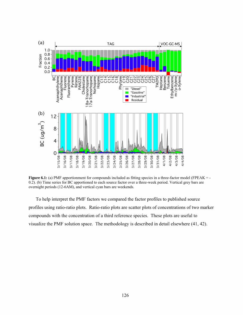
126
Figure 6.1: (a) PMF apportionment for compounds included as fitting species in a three-factor model (FPEAK = -0.2). (b) Time series for BC apportioned to each source factor over a three-week period. Vertical grey bars are overnight periods (12-6AM), and vertical cyan bars are weekends.
To help interpret the PMF factors we compared the factor profiles to published source
profiles using ratio-ratio plots. Ratio-ratio plots are scatter plots of concentrations of two marker
compounds with the concentration of a third reference species. These plots are useful to
visualize the PMF solution space. The methodology is described in detail elsewhere (41, 42).
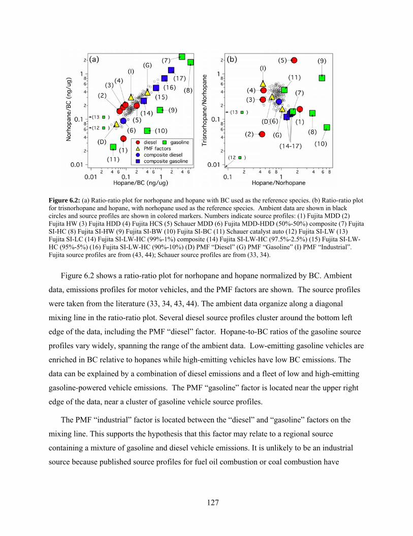
127
Figure 6.2: (a) Ratio-ratio plot for norhopane and hopane with BC used as the reference species. (b) Ratio-ratio plot for trisnorhopane and hopane, with norhopane used as the reference species. Ambient data are shown in black circles and source profiles are shown in colored markers. Numbers indicate source profiles: (1) Fujita MDD (2) Fujita HW (3) Fujita HDD (4) Fujita HCS (5) Schauer MDD (6) Fujita MDD-HDD (50%-50%) composite (7) Fujita SI-HC (8) Fujita SI-HW (9) Fujita SI-BW (10) Fujita SI-BC (11) Schauer catalyst auto (12) Fujita SI-LW (13) Fujita SI-LC (14) Fujita SI-LW-HC (99%-1%) composite (14) Fujita SI-LW-HC (97.5%-2.5%) (15) Fujita SI-LW-HC (95%-5%) (16) Fujita SI-LW-HC (90%-10%) (D) PMF “Diesel” (G) PMF “Gasoline” (I) PMF “Industrial”. Fujita source profiles are from (43, 44); Schauer source profiles are from (33, 34).
Figure 6.2 shows a ratio-ratio plot for norhopane and hopane normalized by BC. Ambient
data, emissions profiles for motor vehicles, and the PMF factors are shown. The source profiles
were taken from the literature (33, 34, 43, 44). The ambient data organize along a diagonal
mixing line in the ratio-ratio plot. Several diesel source profiles cluster around the bottom left
edge of the data, including the PMF “diesel” factor. Hopane-to-BC ratios of the gasoline source
profiles vary widely, spanning the range of the ambient data. Low-emitting gasoline vehicles are
enriched in BC relative to hopanes while high-emitting vehicles have low BC emissions. The
data can be explained by a combination of diesel emissions and a fleet of low and high-emitting
gasoline-powered vehicle emissions. The PMF “gasoline” factor is located near the upper right
edge of the data, near a cluster of gasoline vehicle source profiles.
The PMF “industrial” factor is located between the “diesel” and “gasoline” factors on the
mixing line. This supports the hypothesis that this factor may relate to a regional source
containing a mixture of gasoline and diesel vehicle emissions. It is unlikely to be an industrial
source because published source profiles for fuel oil combustion or coal combustion have

128
extremely high hopane-to-BC ratios and would appear in the top right corner of a ratio-ratio plot
off the scale of Figure 6.2.
6.3 CMB Analysis
CMB analysis was performed to estimate ambient concentrations of diesel particulate matter.
Ambient concentrations of BC and several hopanes (norhopane, hopane, cholestane,
trisnorhopane and homohopane isomers) were fit by CMB using one diesel and one gasoline
vehicle source profile. Different combinations of gasoline and diesel source profiles were fit to
quantify the uncertainty in the solution due to source profile variability. The CMB analysis was
performed on data from 177 samples. All CMB solutions had acceptable statistical performance,
with average r2 > 0.82 and χ2 < 1.
The CMB anlaysis considered three different diesel source profiles: a composite medium-
duty diesel profile (profile #1 in Figure 6.2), a composite heavy-duty diesel profile (profile #3 in
Figure 6.2), and an emissions-weighted average of these two profiles (profile #6 in Figure 6.2).
Only one diesel profile is fit at a time by the CMB model. To apportion gasoline vehicle
emissions, we examined vehicle fleets with different amounts of low- and high-emitting vehicles.
This was done by creating composite profiles using the low- and high-emitting profiles plotted in
Figure 6.3 (profiles #12 and #6 or #8). Separate CMB models considered vehicle fleets of 1%,
2.5%, 5%, and 10% high emitters (profiles #14-17 in Figure 6.3).
Figure 6.3: Comparison of PMF and CMB apportionment of black carbon (BC) to (a) diesel and (b) gasoline vehicles. Results are shown CMB solutions with different composite gasoline profiles, as discussed in the text.

129
Figure 6.3 shows scatter plots for BC apportioned by PMF to the mobile source factors
versus BC apportioned by CMB to the gasoline and diesel source profiles. Results from several
CMB scenarios are shown; each scenario used the same composite diesel profile (#6) paired
with a different composite gasoline profile (#14-17 and #7). All of the different models
apportion roughly the same fraction BC to diesel vehicles (m = 0.98 - 1.02, r2 = 0.88 - 0.94),
indicating that the solutions are well constrained. The BC apportioned to gasoline vehicles by
the different models usually agrees to within a factor of two, with many data points clustered
around the 1:1 line for the 1 to 5% high-emitter scenarios.
The good agreement between the PMF and CMB solutions provides confidence in the source
apportionment results, especially for diesel vehicles. Each CMB model also provides an
estimate of the study-average DPM concentrations in downtown Pittsburgh. These estimates
ranged from 3.0 to 4.3 μg m-3. Figure 6.4 presents the CMB results as a histogram to illustrate
the variability in the DPM estimates.
CMB analysis was also performed using archived hopanes and BC data measured in
Schenley Park as part of the Pittsburgh Air Quality Study (6). This site is considered an “urban
background” site not strongly influenced by local sources. The DPM estimates for the Schenley
Park site are presented in Figure 6.4. These are based on the same combinations of source
profiles used for the analysis of the downtown data. In Schenley Park, annual average DPM
concentrations range from 0.8 to 1.1 g m-3, which are more than a factor of three lower than
those at the Diamond Building. This underscores that the downtown area is strongly influenced
by diesel vehicle emissions.
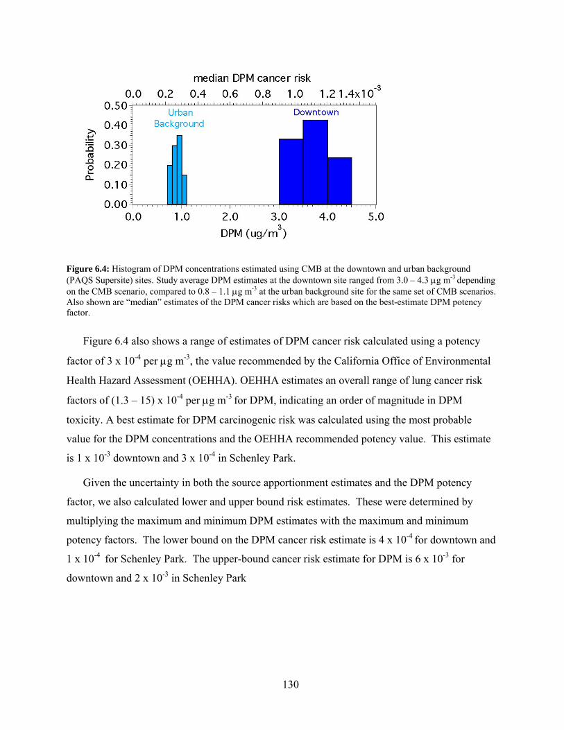
130
Figure 6.4: Histogram of DPM concentrations estimated using CMB at the downtown and urban background (PAQS Supersite) sites. Study average DPM estimates at the downtown site ranged from 3.0 – 4.3 g m-3 depending on the CMB scenario, compared to 0.8 – 1.1 g m-3 at the urban background site for the same set of CMB scenarios. Also shown are “median” estimates of the DPM cancer risks which are based on the best-estimate DPM potency factor.
Figure 6.4 also shows a range of estimates of DPM cancer risk calculated using a potency
factor of 3 x 10⁻⁴ per g m-3, the value recommended by the California Office of Environmental
Health Hazard Assessment (OEHHA). OEHHA estimates an overall range of lung cancer risk
factors of (1.3 – 15) x 10-4 per g m-3 for DPM, indicating an order of magnitude in DPM
toxicity. A best estimate for DPM carcinogenic risk was calculated using the most probable
value for the DPM concentrations and the OEHHA recommended potency value. This estimate
is 1 x 10⁻³ downtown and 3 x 10⁻⁴ in Schenley Park.
Given the uncertainty in both the source apportionment estimates and the DPM potency
factor, we also calculated lower and upper bound risk estimates. These were determined by
multiplying the maximum and minimum DPM estimates with the maximum and minimum
potency factors. The lower bound on the DPM cancer risk estimate is 4 x 10⁻⁴ for downtown and
1 x 10⁻⁴ for Schenley Park. The upper-bound cancer risk estimate for DPM is 6 x 10⁻³ for
downtown and 2 x 10⁻³ in Schenley Park

131
Chapter 7. Risk Synthesis: Apportioning Risks to Sources in Allegheny County
In previous chapters, Positive Matrix Factorization (PMF) was used to apportion a subset of
gas phase organic air toxics to sources and the Chemical Mass Balance (CMB) model was used
to estimate the ambient concentrations of diesel particulate matter. This chapter first discusses
the sources of air toxics not included in these models and then all of the results are combined to
apportion cancer risks to source classes. Metals are also an important subset of air toxics, but not
enough information is available on the sources in Allegheny County to include them in the
analysis.
7.1 Apportioning Risks from Air Toxics not included in PMF
Several air toxics that contribute substantial risk were not included in the PMF or CMB
models because they did not vary temporally or were not measured during the intensive
campaigns. This section discusses the apportionment of formaldehyde, carbon tetrachloride,
acetaldehyde, 1,3-butadiene, hexachlorobutadiene, vinyl chloride, benzyl chloride and acrolein.
7.1.1 Formaldehyde
Of the gas-phase organic air toxics considered by this study, formaldehyde contributes the
largest cancer risk throughout Allegheny County, 33%-48% of the additive cancer risk with the
highest relative contribution at the regional background site.
Formaldehyde is emitted by point and mobile sources as well as formed in the atmosphere
from the oxidation of hydrocarbons (21). Previous research has found that secondary formation
of formaldehyde is often more important than primary emissions (45) and data from the four
baseline sites lead to the same conclusion for Allegheny County. First, formaldehyde
concentrations were about a factor of two higher during the summer than during any other season
(Figure 4.12) – a clear indication of secondary production. Second, two statistical tests indicate
that formaldehyde is primarily a regional pollutant in Allegheny County that is not strongly
influenced by local emissions. First the bootstrap method was used to compare the study-
average concentrations measured at the four baseline studies. For the Stowe, South Fayette and

132
Flag Plaza sites, the null hypothesis that the study-average concentrations were the same could
not be rejected at the 95th percentile level. This means that study-average concentrations at
Stowe, South Fayette, and Flag Plaza are not statistically different from each other. However,
for Avalon the null hypothesis could be rejected, meaning that the mean concentration at Avalon
could be different than the mean concentration at the other sites. Formaldehyde concentrations
in Avalon were 17% higher (0.45 g/m3) than in South Fayette, with 95% confidence intervals
for this difference of 0.17 to 0.71g/m3. Therefore, local emissions appear to contribute
modestly to formaldehyde exposures in Avalon.
The second statistical test was to compare the linear correlation between formaldehyde
measured at different sites to correlations of formaldehyde with other pollutants measured at the
same site. Formaldehyde concentrations in Avalon and Flag Plaza are more strongly correlated
with formaldehyde concentrations in South Fayette than with other pollutants from the same site,
further supporting the conclusion that formaldehyde is a regional pollutant. In Stowe,
formaldehyde concentrations were most correlated with other carbonyls (acetaldehyde, acetone,
and acrolein) measured at the Stowe site than with formaldehyde in South Fayette. This
potentially indicates a local source of carbonyls in Stowe, but may simply be due to
concentrations of this set of secondary pollutants co-varying in time.
Based on this analysis, 100% of the formaldehyde will be apportioned to regional/secondary
sources at the regional background site (South Fayette), and downtown (Flag Plaza). At Avalon
83% of formaldehyde was apportioned to regional/secondary sources and 17% apportioned to
local, industrial emissions.
7.1.2 Carbon tetrachloride
Carbon tetrachloride contributes 9%-12% of the total cancer risk in Allegheny County. Its
concentration and absolute risk did not vary between the four sites. High time resolved
measurements showed little to no temporal variation at any of the sites. Therefore, carbon
tetrachloride is a regional pollutant.
Carbon tetrachloride is a CFC that was used extensively in the early part of the 20th century
as a refrigerant that was largely banned by the Montreal Protocol. It is currently used in small
quantities as an industrial solvent (21), and there are negligible emissions of carbon tetrachloride

133
in Allegheny County (1). Carbon tetrachloride has a relatively long atmospheric lifetime on the
order of 30-50 years (21), which means that outdoor exposures in Allegheny County today to
carbon tetrachloride are due to historical emissions across the globe. Therefore, carbon
tetrachloride was classified as regional/secondary pollutant at all sites and 100% of carbon
tetrachloride risks were assigned to secondary/background sources.
7.1.3 Acetaldehyde
Acetaldehyde contributes 4%-6% of the cancer risk attributed to the target organic air toxics
throughout Allegheny County. Acetaldehyde is emitted by chemical processing, mobile sources
such as automobiles, tobacco smoke, and is a natural product of combustion and reactions of
other hydrocarbons in the atmosphere (21).
Only a small set of high time resolved data were available from this study to investigate the
sources of acetaldehyde. A previous study attributed 40% of the acetaldehyde from mobile
sources and 60% from atmospheric production at an urban background site in Pittsburgh
(Schenley Park) (7). We assumed the same split for the South Fayette data, apportioning 0.65
g/m3 of acetaldehyde to mobile-source emissions and 0.94 g/m3 to secondary production.
Furthermore, we assumed that the regional/secondary contribution would be the same at all sites,
0.94 g/m3, and that any excess acetaldehyde was due to mobile source emissions. This may
somewhat overestimate the mobile source contribution in Avalon, the site with the highest
acetaldehyde concentrations. In Avalon some of the emissions from industrial sources may also
be important, but this uncertainty is small, affecting less than 10% of the acetaldehyde risks. The
risks apportionments were: Avalon 58% mobile, 42% background/ secondary; downtown 54%
mobile, 46% background/secondary; background 40%mobile, 60% background/secondary.
7.1.4 1,3-butadiene
1,3-butadiene contributes 3%-6% of the gas-phase organic air toxics cancer risk in Allegheny
County. Although 1,3-butadiene is one of the top ten risk contributors, concentrations of 1,3-
butadiene in Allegheny County are at the national average at the three urban baseline sites and
below the 25th percentile at the regional background site (Figures 3.1 and 3.2). 1,3 butadiene is
emitted from mobile vehicles, cooking, and point sources that produce/use polymers (21, 33, 35).

134
High time resolved measurements of 1,3-butadiene were taken at Avalon and downtown.
1,3-butadiene was included in the downtown PMF model but not the Avalon model because the
Avalon 1,3 butadiene dataset was incomplete. The downtown PMF results apportioned 65% of
the 1,3 butadiene to the downtown factor, which is thought to be mobile diesel, and 24% from
the southeastern factor, which is thought to be a mixture gasoline vehicle and industrial
emissions from the Clairton area. Since there are no reported industrial emissions of 1,3
butadiene from the Clairton area, all of the 1,3 butadiene in southeastern factor was attributed to
mobile sources.
Concentrations of 1,3-butadiene at Avalon are slightly higher than in downtown. The
Neville Chemical Company near Avalon reports 110 kg of 1,3-butadiene emissions per year (1).
At the Avalon site it was assumed that the increase in concentration was from non-mobile
sources. At Avalon 88% of the 1,3-butadiene is from mobile sources and 12% of the 1,3-
butadiene is from non-mobile sources, specifically industry. It was assumed that 100% of the 1,3
butadiene is from mobile sources at the background site, South Fayette.
7.1.5 Hexachlorobutadiene, 1,2-Dichloropropane, and Vinyl Chloride
Hexachlorobutadiene, 1,2-dichloropropane, and vinyl chloride concentrations were similar at
all four baseline sites. Therefore all of these species were apportioned to regional emissions at
each site.
7.1.6 Acrolein
Acrolein is the only air toxic estimated to pose a non-cancer risk in Allegheny County.
Although the hazard quotient of acrolein is above one at all of the sites, acrolein concentrations
in Allegheny County are low compared to the rest of the nation (Figure 3.3). Baseline
measurements showed that acrolein concentrations were a factor of two higher at the urban sites
as compared to South Fayette with highest concentrations at Avalon and Stowe.
Acrolein is emitted by manufacturing processes and in combustion exhaust (21). At South
Fayette acrolein did not correlate very strongly with any other pollutants. At Avalon and Stowe
acrolein correlates most highly with carbon disulfide and styrene, two tracers of emissions from
industrial facilities on Neville Island. According to the inventory there are no significant sources

135
of acrolein on Neville Island, but that does not appear to be the case. Given the current data set it
is difficult to apportion acrolein to sources.
7.2 Apportionment of Risks to Sources
Results from the PMF apportionment of air toxics, the DPM concentration calculations, and
the apportionment of air toxics in this chapter were combined to apportion risks to source
classes. Figures 7.1 to 7.3 shows the apportionment of risks at all sites for sources class, origins
of risks and apportionment of non-mobile risks. For the 36 target organic air toxics,
regional/secondary pollutants, mainly formaldehyde and carbon tetrachloride, are the dominant
contributor to the cancer risk at each site. Non-mobile sources are the second largest contributor
followed mobile-source emissions.
Figure 7.4 combines the risk estimates for gas-phase organic air toxics with estimates for
diesel PM (DPM). DPM estimates were only available for the downtown and urban background
sites. Given the modest spatial variation in BC concentrations outside of the downtown area
(Figure 3.4), it was assumed that the Avalon diesel PM risk was equal to the background diesel
PM risk. When diesel PM is included in the analysis, Figure 7.4 indicates mobile source risks
are much greater than all of the other source classes.
In Chapter 3 it was shown that the metals risks were one third to one half the magnitude of
additive cancer risks attributed to the organic air toxics. Not enough is known about the metals
apportionment in Allegheny County to include them in this apportionment. DPM would still
dominate risks even if metals were included and therefore mobile sources would still dominate
risk contributions. Adding metals may alter the relative importance of non-mobile to
regional/background sources.

136
0.0E+00
2.0E-05
4.0E-05
6.0E-05
8.0E-05
1.0E-04
Origin ofApportioned
Risks
Source Class ofApportioned
Risks
Apportionment ofNon-MobileSources
Ca
nc
er
LIR
(L
ife
tim
e In
cid
en
ce
Ra
te)
Neville Island
Non-Neville
Background/ Secondary
Non-Mobile
Mobile
Unknown
Unknown
Coke Works
Chemical Plants
ACSA
Figure 7.1 Source apportionment of the additive cancer risk for the 36 target gas-phase organic air toxics at the Avalon site.

137
0.0E+00
3.0E-05
6.0E-05
9.0E-05
1.2E-04
Origin ofApportioned
Risks
Source Class ofApportioned
Risks
Apportionment ofNon-MobileSources
Ca
nc
er
LIR
(L
ife
tim
e In
cid
en
ce
Ra
te)
Downtown
Non-Local
Background/ Secondary
Non-Mobile
Mobile
Unknown
Unknown
Coke Works
UpRiver
Dry Cleaning
Figure 7.2 Source apportionment of the additive cancer risk for 36 target gas-phase organic air toxics in downtown Pittsburgh.

138
0.0E+00
1.0E-05
2.0E-05
3.0E-05
4.0E-05
5.0E-05
6.0E-05
7.0E-05
8.0E-05
Origin ofApportioned Risks
Source Class ofApportioned Risks
Apportionment ofNon-MobileSources
Ca
nc
er
LIR
(L
ife
tim
e In
cid
en
ce
Ra
te)
Local
Non-Local
Background/ Secondary
Non-Mobile
Mobile
Unknown
Unknown
Coke Works
Up River Industry
Figure 7.3 Source apportionment of the additive cancer risk for 36 target gas-phase organic air toxics in South Fayette.

139
0.0E+00 3.0E-04 6.0E-04 9.0E-04 1.2E-03
Downtown
Avalon
Background
Cancer LIR (Lifetime Incidence Rate)
Regional and SecondaryNon-Mobile SourcesMobile Sources
Figure 7.4 Additive cancer for gas-phase organic air toxics and DPM for each of the sites divided into regional/secondary contribution, mobile source contribution, and industrial contribution.
7.3 Conclusions
If only gas-phase organic air toxics are considered, background/regional sources dominate
the risk profile. Non-mobile gas phase risks were dominated by risks associated with coke works
emissions, primarily from benzene, at the Avalon site. At the downtown site non-mobile risks
were dominated by point source emissions of chlorinated compounds, specifically
trichloroethene. The sources of these chlorinated compounds are unknown.
Including diesel particulate matter in the risks apportionment dramatically changes the
results. DPM risks are greater than gas phase risks at each of the sites making mobile sources by
far the most dominate source class. The highest contributions to risks were seen downtown.

140
Chapter 8. Evaluating NATA: Comparison of predicted and measured air toxic concentrations, sources, and risks
The Government Performance and Results Act set a goal of reducing air toxic emissions by
75% from the 1993 levels (46). In order to make informed policy decisions, air toxic
concentrations, sources, and risks throughout the nation need to be determined. To help achieve
this goal, the EPA conducted the National Air Toxics Assessment (NATA). The initial
assessment estimated exposures and risks of 33 of the 189 air toxics at the census track level
throughout the county using an integrated emissions, dispersion, exposure and risk modeling
framework. In 1999 NATA was expanded to include 177 pollutants. EPA is currently working
on the 2002 NATA.
NATA consists of four main components: compiling a national emissions inventory of
outdoor sources, modeling annual average outdoor concentrations of air toxics at the census tract
level, determining human exposure to outdoor air toxics, and finally estimating health risks
associated with inhalation of air toxics. Critical inputs are the National Toxics Inventory (NTI),
meteorology and topographical data, NATA simulates pollutant dispersion and chemical reaction
during transport using a version of AERMOD that has been implemented as part of the
Assessment System for Population Exposure Nationwide (ASPEN) (47).
NATA estimates the concentration, sources, and health risks of air toxics at the census tract
level throughout Allegheny County. The NATA results can be used to prioritize pollutants and
emissions sources and indentify potential air toxic hotspots. Therefore, the NATA
source/inventory-based estimates of risks complement the receptor/ambient concentration based
estimates that are the focus of this study. However, relatively few studies have compared
predictions of the NATA modeling framework to measured concentrations (48, 49), and no
evaluations have been conducted in Allegheny County. The published comparisons have shown
that measured and predicted concentrations of gas-phase primary emissions are generally within
a factor of 10. Larger discrepancies exist for regional and secondary pollutants. Previous studies
have not evaluated the predicted source contributions or risks rankings.
In this chapter, predictions of the 2002 National Air Toxics Assessment (NATA) are
evaluated using the experimental data. Measured concentrations are compared to census tract

141
level predictions at the four baseline sites. The pollutant risk ranking from Chapter 3 is
compared to the risks calculated from the NATA-modeled outdoor concentrations. Finally, the
source apportionment results from Chapter 5 and 7 are compared to the NATA source
apportionment. The chapter concludes with a brief discussion of how these comparisons refine
our understanding of the sources and risks of air toxics in Allegheny County.
8.1 Target Air Toxics
This analysis investigated NATA performance for 47 air toxics listed in Table 8.1. This
includes 37 gas phase organic air toxics, 10 metals, and all of the priority air toxics identified in
Chapter 3.
Table 8.1 also indicates air toxics which are considered in each component of the evaluation.
Predicted concentrations of each toxic are compared to measure data. All of the toxics with
health risk data, RFC or UREs, were included in the risk ranking analysis. The source
apportionment comparison focused on air toxics that pose substantial health risks.
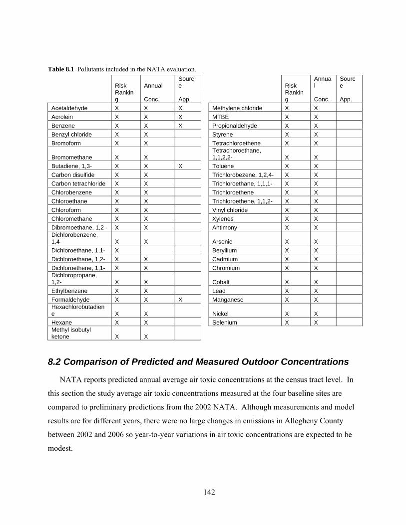
142
Table 8.1 Pollutants included in the NATA evaluation.
Risk Annual Source Risk
Annual
Source
Ranking Conc. App.
Ranking Conc. App.
Acetaldehyde X X X Methylene chloride X X
Acrolein X X X MTBE X X
Benzene X X X Propionaldehyde X X
Benzyl chloride X X Styrene X X
Bromoform X X Tetrachloroethene X X
Bromomethane X X Tetrachoroethane, 1,1,2,2- X X
Butadiene, 1,3- X X X Toluene X X
Carbon disulfide X X Trichlorobezene, 1,2,4- X X
Carbon tetrachloride X X Trichloroethane, 1,1,1- X X
Chlorobenzene X X Trichloroethene X X
Chloroethane X X Trichloroethene, 1,1,2- X X
Chloroform X X Vinyl chloride X X
Chloromethane X X Xylenes X X
Dibromoethane, 1,2 - X X Antimony X X Dichlorobenzene, 1,4- X X Arsenic X X
Dichloroethane, 1,1- X Beryllium X X
Dichloroethane, 1,2- X X Cadmium X X
Dichloroethene, 1,1- X X Chromium X X Dichloropropane, 1,2- X X Cobalt X X
Ethylbenzene X X Lead X X
Formaldehyde X X X Manganese X X Hexachlorobutadiene X X Nickel X X
Hexane X X Selenium X X Methyl isobutyl ketone X X
8.2 Comparison of Predicted and Measured Outdoor Concentrations
NATA reports predicted annual average air toxic concentrations at the census tract level. In
this section the study average air toxic concentrations measured at the four baseline sites are
compared to preliminary predictions from the 2002 NATA. Although measurements and model
results are for different years, there were no large changes in emissions in Allegheny County
between 2002 and 2006 so year-to-year variations in air toxic concentrations are expected to be
modest.

143
Figures 8.1 to 8.3 present scatter plots of predicted annual average outdoor concentration
versus the measured geometric mean concentration for 29 air toxics. The error bars extend to the
95th percentile confidence interval of the mean. There is reasonable agreement between the
measured and predicted concentrations. The best agreement is observed for carbon tetrachloride,
chloromethane, bromomethane, and chloroform. Measured and predicted concentrations of these
four pollutants rest almost on the 1:1 line on the scatter plots. Measured and predicted
concentrations of acetaldehyde, benzene, formaldehyde, xylenes, toluene, tetrachloroethene,
acrolein, ethylbenzene and hexane are generally within a factor of two at all sites. Measured and
predicted 1,3-butadiene, tetrachloroethene, 1,4-dichlorobenzene, trichloroethene, 1,2
dibromoethane, and 1,2 dichloromethane concentrations are within a factor of two at three sites
but at one site concentrations differ by more than a factor of two. Measured concentrations of
MTBE, 111-trichloroethene, and MIBK were lower than the modeled concentrations by at least a
factor of two at all sites.
Figures 8.1-8.3 reveal poor model performance for some air toxics. Measured concentrations
of carbon disulfide, styrene, propionaldehyde, vinyl chloride, 1,2-dichloroethane, and
chlorobenzene were consistently higher than modeled concentrations by at least a factor of two at
all sites. Styrene was underpredicted by a factor of six at both Avalon and Stowe, the two sites
next to Neville Island. Propionaldehyde was underpredicted by at least a factor of two at all sites
and by a factor of four at the urban background site (South Fayette). 1,2-dichoroethane was
underpredicted by a factor of 10-12 at all sites. Vinyl Chloride was underpredicted by a factor of
20 at Flag Plaza. Chlorobenzene concentrations are 16-30 times higher than the modeled values.
Carbon disulfide concentrations were 15 times higher than predicted concentrations at Avalon
and Stowe and 58 times higher downtown (Flag Plaza).
The predicted concentrations of the remaining eight air toxics were essentially zero (<1.0 x
10-4 g/m3). These eight toxics are: chloroethane, 1,1-dichloroethene, 1,1-dichloroethane,
bromoform, benzyl chloride, 1,2,4-trichlorobenzene, and hexachlorobutadiene. All of these
pollutants had concentrations less than 0.015 g/m3 at all sites, however concentrations were
high enough for cancer risks to be greater than one in a million at all sites for
hexachlorobutadiene and at three sites for benzyl chloride.

144
0
1
2
3
4
5
6
7
8
0 2 4 6 8
Modeled Conc. (g/m3)
Me
as
ure
d C
on
c. (
g/m
3 )CarbontetrachlorideChloromethane
Acetaldehyde
Benzene
Formaldehyde
Xylenes
Toluene
1:1
1:2
2:1
0
0.2
0.4
0.6
0 0.1 0.2 0.3 0.4
Modeled Conc. (g/m3)
Me
as
ure
d C
on
c. (
g/m
3 )
Bromomethane
Chloroform
Acrolien
Butadiene, 1,3-
MTBE
Trichloroethene,1,1,1-Carbon disulfide
Tetrachoroethene
2:1
1:1
1:2
Figure 8.1 Comparison of measured and predicted annual average concentrations of gas-phase organic air toxics.

145
0
0.5
1
1.5
2
2.5
3
0 0.2 0.4 0.6 0.8 1 1.2
Modeled Conc. (g/m3)
Me
as
ure
d C
on
c. (
g/m
3 )
Styrene
Ethylbenzene
Trichloroethene
Dichlorobenzene,1,4-Hexane
Propionaldehyde
MIBK
MethyleneChloride
2:1
1:2
1:1
0
0.01
0.02
0.03
0.04
0.05
0 0.002 0.004 0.006 0.008 0.01
Moldeled Conc. (g/m3)
Mea
sure
d C
on
c. (g
/m3 )
Vinyl chloride
Dibromoethane,1,2-Tetrachoroethane,1,1,2,2-Dichloropropane,1,2-Chlorobenzene
Dichloroethane,1,2-Trichoroethane,1,1,2-
2:1
1:2
1:1
Figure 8.2 Comparison of measured and predicted annual average concentrations of selected gasphase organic air toxics.
Figure 8.3 presents scatter plots of measured versus predicted concentrations for metals at
two sites -- Avalon and Schenley Park. Measured concentrations of most of the metals, with the
exception of beryllium and arsenic, were underestimated at all of the sites. For example, arsenic
concentrations are underestimated at Avalon by about a factor of two.
Modeled Concentration (g/m3)

146
0
0.005
0.01
0.015
0.02
0.025
0.03
0 0.01 0.02 0.03
Modeled Conc. (g/m3)
Me
as
ure
d C
on
c. (
g/m
3 )Antimony
Arsenic
Beryllium
Cadmium
Chromium
Cobalt
Lead
Manganese
Nickel
Selenium
2:1 1:1
1:2
0
0.0005
0.001
0.0015
0.002
0.0025
0.003
0.0035
0.004
0.0045
0.005
0 0.001 0.002 0.003 0.004 0.005
Modeled Conc. (g/m3)
1:2
2:1 1:1
Figure 8.3 Measured versus modeled concentrations for metals measured at Avalon and Schenley Park sites.
Overall the level of agreement between the NATA predicted and measured air toxic
concentrations in Allegheny County is comparable to other areas in the country (48, 49) The
results suggest that emissions inventories of the modeled dispersion of chlorinated compounds
need to be significantly improved as well as for carbon disulfide, styrene, and propionaldehyde.
Of the 22 air toxics identified as priority air toxics in Section 3.5, measured and predicted
concentrations for 12 were found to be within a factor of two. However, NATA substantially
overpredicts MIBK concentrations and NATA severely underpredicts concentrations of 3
chlorinated air toxics (trichloroethene, 1,4-dichlorobenzene, and methylene chloride) at the Flag
Plaza site, indicating problems with inventories in this specific area of the county. 1,3 butadiene
is also underpredicted at the South Fayette site. Finally, five air toxics (hexachlorobutadiene,
benzyl chloride, 1,2-dichloroethane, propionaldehyde, and styrene) were systematically
underpredicted at all of the sites, indicting more widespread inventory problems. These are
important non-mobile sources of these compounds including industry, biomass burning, and
solvent use.
8.3 Risk Ranking of Pollutants
One of the intended uses of NATA is to identify priority or high risk air toxics (50). In
Chapter 3 the cancer and non-cancer risks were estimated using measured concentrations. In this
section, the same risk model is applied to the NATA predicted outdoor concentrations and the
two sets of risk estimates are compared. Although outdoor concentrations are only one
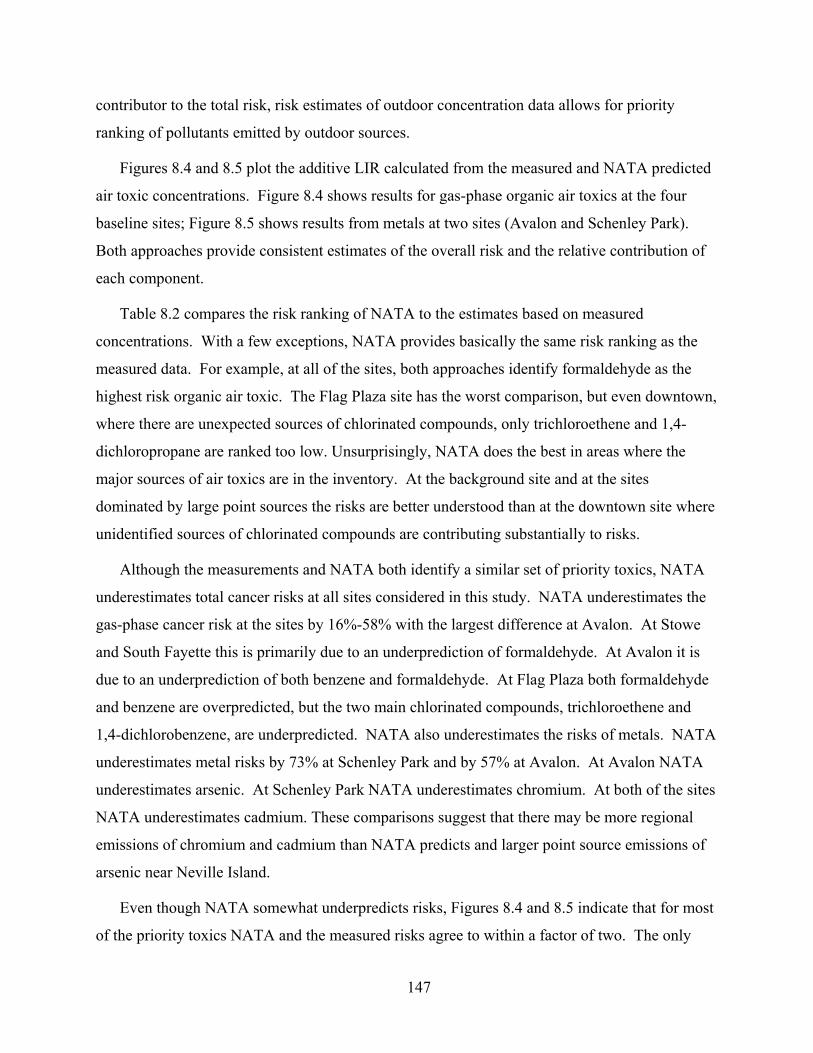
147
contributor to the total risk, risk estimates of outdoor concentration data allows for priority
ranking of pollutants emitted by outdoor sources.
Figures 8.4 and 8.5 plot the additive LIR calculated from the measured and NATA predicted
air toxic concentrations. Figure 8.4 shows results for gas-phase organic air toxics at the four
baseline sites; Figure 8.5 shows results from metals at two sites (Avalon and Schenley Park).
Both approaches provide consistent estimates of the overall risk and the relative contribution of
each component.
Table 8.2 compares the risk ranking of NATA to the estimates based on measured
concentrations. With a few exceptions, NATA provides basically the same risk ranking as the
measured data. For example, at all of the sites, both approaches identify formaldehyde as the
highest risk organic air toxic. The Flag Plaza site has the worst comparison, but even downtown,
where there are unexpected sources of chlorinated compounds, only trichloroethene and 1,4-
dichloropropane are ranked too low. Unsurprisingly, NATA does the best in areas where the
major sources of air toxics are in the inventory. At the background site and at the sites
dominated by large point sources the risks are better understood than at the downtown site where
unidentified sources of chlorinated compounds are contributing substantially to risks.
Although the measurements and NATA both identify a similar set of priority toxics, NATA
underestimates total cancer risks at all sites considered in this study. NATA underestimates the
gas-phase cancer risk at the sites by 16%-58% with the largest difference at Avalon. At Stowe
and South Fayette this is primarily due to an underprediction of formaldehyde. At Avalon it is
due to an underprediction of both benzene and formaldehyde. At Flag Plaza both formaldehyde
and benzene are overpredicted, but the two main chlorinated compounds, trichloroethene and
1,4-dichlorobenzene, are underpredicted. NATA also underestimates the risks of metals. NATA
underestimates metal risks by 73% at Schenley Park and by 57% at Avalon. At Avalon NATA
underestimates arsenic. At Schenley Park NATA underestimates chromium. At both of the sites
NATA underestimates cadmium. These comparisons suggest that there may be more regional
emissions of chromium and cadmium than NATA predicts and larger point source emissions of
arsenic near Neville Island.
Even though NATA somewhat underpredicts risks, Figures 8.4 and 8.5 indicate that for most
of the priority toxics NATA and the measured risks agree to within a factor of two. The only

148
high priority toxic in Allegheny County that NATA does poorly with is trichloroethene. NATA
underpredicts the risks posed by trichloroethylene at the Flag Plaza site by more than a factor of
10. NATA also underpredicts cadmium and lead by more than a factor of five and seven
respectively, but these toxics pose lower risks. This indicates problems with either the emissions
inventories or dispersion of these compounds in the model; however, these problems do not
radically alter the conclusions one would derive from NATA.
Since the cancer unit risk estimates (URE) vary widely from toxic to toxic, NATA can
accurately prioritize risks without precisely predicting outdoor concentrations for all air toxics.
In order to accurately predict risks, NATA must accurately predict concentrations of the risk
drivers. NATA predictions for priority air toxics are generally within a factor of two; therefore it
gets the overall risks and risks rankings basically right. With the exception of the chlorinated
compounds at Flag Plaza, the air toxics that NATA does a poor job of predicting are not risks
drivers and therefore do not significantly alter conclusions regarding risk reduction priorities.
Therefore, when evaluated on a risk basis, NATA performance is better than when it is
considered on a concentration basis.
For non-cancer risks both approaches found that acrolein was the only air toxic that had a
hazard quotient larger than one. Therefore, both approaches identified acrolein as the only air
toxic potentially posing any non-cancer risks.
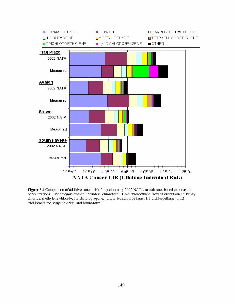
149
Figure 8.4 Comparison of additive cancer risk for preliminary 2002 NATA to estimates based on measured concentrations. The category “other” includes: chloroform, 1,2-dichloroethane, hexachlorobutadiene, benzyl chloride, methylene chloride, 1,2-dicloropropane, 1,1,2,2-tetrachloroethane, 1,1-dichloroethane, 1,1,2-trichloroethane, vinyl chloride, and bromoform.

150
Figure 8.5 Comparison of additive cancer risk for preliminary 2002 NATA to estimates based on measured concentrations for metals.

151
Table 8.2 Risk ranking of air toxics from highest cancer risks to lowest for the 10 risk drivers from NATA and the health risks analysis presented in Chapter 3.
South Fayette Avalonrisk ranking Measured Modeled Measured Modeled
1 Formaldehyde Formaldehyde Formaldehyde Formaldehyde2 Benzene Benzene Benzene Benzene3 Carbon tetrachloride Carbon tetrachloride Chromium Chromium4 Chromium Chromium Carbon tetrachloride Carbon tetrachloride5 Arsenic Arsenic 1,3-butadiene Arsenic6 Acetaldehyde 1,3-butadiene Arsenic Acetaldehyde7 Chloroform Acetaldehyde Acetaldehyde 1,3-butadiene8 1,3-butadiene Chloroform Tetrachloroethene Chloroform9 Hexachlorbutadiene Trichloroethene Chloroform Trichloroethene
10 benzy Chloride Tetrachloroethene 1,4-dichlorobenzene Tetrachloroethene
Flag Plaza Stowerisk ranking Measured Modeled Measured Modeled
1 Formaldehyde Formaldehyde Formaldehyde Formaldehyde2 Trichloroethene Benzene Benzene Benzene3 Benzene Carbon tetrachloride Carbon tetrachloride Carbon tetrachloride4 1,4-dichlorobenzene 1,3-butadiene Acetaldehyde 1,3-butadiene5 Carbon tetrachloride Acetaldehyde 1,3-butadiene Acetaldehyde6 1,3-butadiene Chloroform Chloroform Chloroform7 Acetaldehyde Trichloroethene 1,4-dichlorobenzene Trichloroethene8 Chloroform Tetrachloroethene Tetrachloroethene Tetrachloroethene9 Tetrachloroethene 1,4-dichlorobenzene Hexachlorobutadiene 1,4-dichlorobenzene
10 Benzyl Chloride 1,1,2,2-Tetrachloroethane Trichloroethene 1,1,2,2-Tetrachloroethene
8.4 Comparison of Source Apportionment Estimates
The development of effective regulatory strategies requires knowing the sources of priority
air toxics. In Chapter 5, receptor modeling was used to apportion the measured concentrations to
sources. NATA determines sources by modeling the dispersion of emissions. The receptor
modeling results were compared to the NATA based source apportionment for nine priority air
toxics (formaldehyde, benzene, 1,3-butadiene, acetaldehyde, trichloroethene, 1,4-
dichlorobenzene, carbon tetrachloride, and tetrachloroethene) and acrolein, the only potential
non-cancer risk. This section discusses two of the air toxics whose receptor-modeled
apportionment and NATA based source apportionment are most divergent, formaldehyde and
benzene, and what this implies about NATA.
NATA apportions air toxics to five source categories: major point sources, area sources, on-
road mobile sources, non-road mobile sources, and background. The receptor model analysis
can be grouped into three source categories: mobile sources, non-mobile sources and
secondary/background sources. To compare the two estimates, the NATA on-road mobile and
non-road mobile source categories were combined to compare with the receptor modeling mobile
category, and the NATA major point sources and area point sources categories were combined to
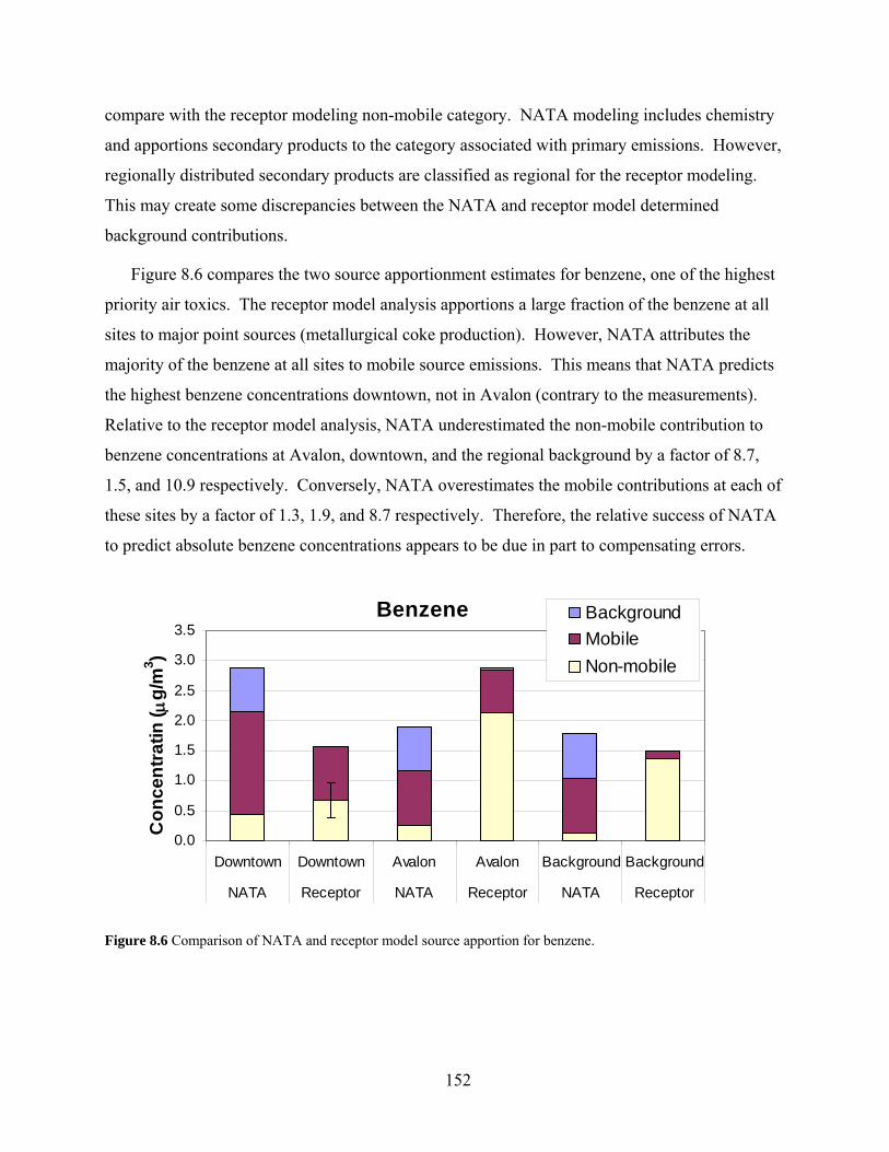
152
compare with the receptor modeling non-mobile category. NATA modeling includes chemistry
and apportions secondary products to the category associated with primary emissions. However,
regionally distributed secondary products are classified as regional for the receptor modeling.
This may create some discrepancies between the NATA and receptor model determined
background contributions.
Figure 8.6 compares the two source apportionment estimates for benzene, one of the highest
priority air toxics. The receptor model analysis apportions a large fraction of the benzene at all
sites to major point sources (metallurgical coke production). However, NATA attributes the
majority of the benzene at all sites to mobile source emissions. This means that NATA predicts
the highest benzene concentrations downtown, not in Avalon (contrary to the measurements).
Relative to the receptor model analysis, NATA underestimated the non-mobile contribution to
benzene concentrations at Avalon, downtown, and the regional background by a factor of 8.7,
1.5, and 10.9 respectively. Conversely, NATA overestimates the mobile contributions at each of
these sites by a factor of 1.3, 1.9, and 8.7 respectively. Therefore, the relative success of NATA
to predict absolute benzene concentrations appears to be due in part to compensating errors.
Benzene
0.0
0.5
1.0
1.5
2.0
2.5
3.0
3.5
Downtown Downtown Avalon Avalon Background Background
NATA Receptor NATA Receptor NATA Receptor
Co
nc
en
tra
tin
(
g/m
3 )
Background
Mobile
Non-mobile
Figure 8.6 Comparison of NATA and receptor model source apportion for benzene.

153
Formaldehyde
0.0
0.5
1.0
1.5
2.0
2.5
3.0
Downtown Downtown Background Background Avalon Avalon
NATA Receptor NATA Receptor NATA Receptor
Co
nce
ntr
atio
n (g
/m3)
Background
Mobile
Non-mobile
Figure 8.7 Comparison of NATA and receptor model apportionment of formaldehyde.
Formaldehyde is another priority mobile source air toxic that NATA appears to overestimate
at mobile dominated sites and underestimate elsewhere. Figure 8.7 indicates large differences
between the two source apportionment estimates for formaldehyde, another priority air toxic. As
discussed in Chapter 3, formaldehyde concentrations are regionally distributed in Allegheny
County. For this reason, we attributed the majority of measured formaldehyde to
secondary/background sources. In contrast, NATA apportions most of the formaldehyde to local
mobile source emissions. NATA also predicts large spatial gradients in formaldehyde
concentrations with levels downtown being about a factor of two higher than the other sites. The
result is that NATA overpredicts formaldehyde concentrations at Flag Plaza and underpredicts
them at the other sites. Therefore, NATA is overestimating local formaldehyde emissions while
underestimating regional secondary production.
In Allegheny County NATA appears to consistently overestimate the mobile source
contribution of two major gas-phase risk contributors and underestimate the non-mobile or
industrial contributions. Although most of the MSATs that were compared showed some
overestimations of the mobile contribution, the magnitude did vary and acrolein, a MSAT with
higher yields in diesel than gasoline vehicles(33, 34), was underestimated by the model. The
discrepancies may be due to emissions factors, vehicle activity, fleet composition, or another
cause. Another interesting MSAT is propionaldehyde. Propionaldehyde is a regionally

154
distributed air toxic with peak concentrations in the fall. Propionaldehyde is also emitted by
biomass combustion, and biomass smoke levels peak in the fall in the Allegheny County(23).
NATA underestimates concentrations by a factor of 2.5-4 at all sites and apportions almost all of
the propionaldehyde to mobile sources. Although no receptor modeling apportionment of
propionaldehyde is available, the seasonal variation shows the likely influence of biomass
burning that may not be captured in the NATA model.
NATA appeared to consistently underestimate non-mobile contributions while often
overpredicting mobile contributions. For the air toxics that are not mobile sources,
tetrachloroethene, trichloroethene, 1,4-dichlorobenzene, this can be seen in an underprediction of
the outdoor concentrations, especially pollutants associated with large point sources. For the
mobile air toxics, like benzene, it results in an overestimation of concentrations in the areas
thought to be mobile dominated and underpredictions in areas thought to be non-mobile
dominated. This conclusion is supported by the concentration comparisons shown in Figures
8.1-8.3. For example, NATA consistently underpredicts concentrations of chlorinated
compounds and many metals; all of these species are associated with emissions from non-mobile
sources.
8.5 Conclusions
When viewed from the perspective of risk, NATA performs well in Allegheny County.
Except for chlorinated compounds at Flag Plaza, NATA more or less correctly ranks air toxic by
risk. This is due to a combination of the large variation in pollutant toxicity and that NATA does
a better job predicting concentrations of the air toxics that drive the risk estimates. However,
there appear to be some problems in the NATA source apportionment.
Presumably if the NATA source apportionment and the receptor modeling agreed well, then
there is a good sense of the sources for these pollutants. Where NATA and receptor modeling
differ shows possible biases in the model. In Allegheny County, NATA underestimates the
emissions and risks associated with large point sources and overestimates the emissions and risks
from mobile sources. This may be due to several factors including underreporting of industrial
emissions, errors in the emissions factors, or problems with dispersion modeling. More work
needs to be done to identify the sources of these discrepancies.

155
Chapter 9. Synthesis, Conclusions and Recommendations
This chapter synthesizes results from throughout the report for priority air toxics, for
important sources, and for the different measurement sites. The chapter concludes with
recommendations for reducing air toxic exposures in Allegheny County and a discussion of
important data gaps.
9.1 Synthesis by Pollutant
This study investigated the concentrations, health risks, and sources of 65 air toxics at seven
sites in Allegheny County. Based on the measured concentrations and estimated risks, a subset
of the investigated air toxics were classified as priority toxics (Table 3.3). Four air toxics were
found to pose cancer risks greater than 1 in 100,000 at one or more of the baseline sites: diesel
particulate matter, formaldehyde, benzene and trichloroethene. These four pollutants were
classified as the highest priority toxics for Allegheny County. The estimated cancer risk for
trichloroethene was greater than 1 in 100,000 only at the Flag Plaza site; the cancer risks for the
other three highest priority toxics were greater than 1 in 100,000 at all four baseline sites.
9.1.1 Diesel Particulate matter (DPM)
Of the 65 air toxics considered in this study, DPM poses the greatest cancer risk at all of the
sites. The best estimates for the DPM cancer risks were 1 x 10⁻³ downtown and 3 x 10⁻⁴ in
Schenley Park. Figure 9.1 compares the estimated cancer risks to other common risks. Although
a risk of 1 x 10⁻³ is well above typical regulatory thresholds for environmental pollutants, 10-4 or
10-6, it is still well below the cancer incidence rate of 1 in 3 for women and 1 in 2 for men in the
United States (51).

156
10
10
10
10
10-3
-4
-5
-6
-7
Car Accident
Fire
Plane Crash
Drowning
Lightning
Flood
Snake Bite
Background DPM
Downtown DPM
Formaldehyde Benzene
Downtown: Trichloroethene
Carbon Tetrachloride Acetaldehyde 1,3-butadiene
Figure 9.1 A comparison of air toxic cancer risks with other common risks.
Although the toxicity data for DPM are more uncertain than data for some other air toxics,
even at its lower bound the cancer risk estimated for DPM was still greater than the best
estimates for the other 65 air toxics considered here. Therefore, reducing DPM exposures should
be given the highest priority.
Only limited data are currently available on the DPM levels in the county. These data
indicate that downtown is a DPM hotspot, with levels that are a factor of three to four higher
than in other areas in the county. However, even outside of the downtown area, DPM levels are
still high enough such that it still poses the greatest cancer risk.
9.1.2 Formaldehyde
Formaldehyde poses the second highest health risk of the 65 air toxics considered by this
project. However the cancer risks associated with formaldehyde are about a factor of ten lower
than the best estimate for DPM.
Formaldehyde is both directly emitted by sources such as motor vehicles and formed in the
atmosphere from oxidation of volatile organic compounds. The strong seasonal variability and
relatively uniform spatial distribution in formaldehyde concentrations observed across the four
baseline sites indicates that the vast majority in Allegheny County comes from regional and/or
secondary sources. Therefore, there is little opportunity for the county to reduce formaldehyde

157
exposures. Federal regulations to limit regional hydrocarbon emissions for ozone control should
help reduce formaldehyde levels in the county.
9.1.3 Benzene
Benzene was the third most important air toxic studied, posing a lifetime cancer risk of 1 to 2
x 10-5. The highest risks were in Stowe and Avalon, the two residential sites adjacent to Neville
Island. Benzene concentrations and health risks in Allegheny County are high compared to the
national data with concentrations near the 75th percentile in downtown and in South Fayette
(regional background site) and at the 95th percentile at Stowe and Avalon. Therefore, there is a
countywide problem with benzene.
Benzene is emitted by both mobile and industrial sources. Emissions from industrial
facilities, in particular coke works, are a very important source of benzene in Allegheny County.
For example, the high time resolved measurements revealed that benzene was frequently
elevated at all three intensive sites when the wind was blowing from either the Clairton or
Shenango Coke Works. In Avalon emissions from the Shenango Coke Works contribute 66% of
the benzene exposure. Downtown is influenced by emissions from both the Shenango and
Clairton Coke Works, which contribute almost 60% of benzene exposure with the balance from
mobile source emissions. At the Carnegie Mellon University site, emissions from the Clairton
Coke works contributed almost 60% of the benzene exposure. The surprisingly high levels of
benzene in South Fayette may largely be due to emissions from outside of Allegheny County.
9.1.4 Chlorinated Compounds
Several chlorinated air toxics posed large cancer risks downtown, but not at the other
baseline sites. At the Flag Plaza site, these chlorinated toxics contributed about 25% of the
cancer risks attributed to the target organic air toxics. Many of these chlorinated compounds are
commonly used as solvents, but this study was not able to identify specific sources for many of
these toxics. They are not emitted by mobile sources. Most of the chlorinated air toxics did not
co-vary, indicating that they are not emitted by the same source. As discussed in Chapter 4,
concentrations of several of these chlorinated toxics were strongly wind-direction dependent,
which provides insight into the location of sources.

158
Trichloroethene: Trichloroethene was estimated to pose a lifetime cancer risk of 2 x 10⁻⁵ at
the Flag site, which is about a factor of twenty higher than the cancer risk it poses at any other
site. The source of trichloroethene is not known. Elevated trichloroethene concentrations were
not observed during the downtown intensive at the Diamond Building or the Flag Plaza sites. No
major sources of trichloroethene emissions are reported in the Allegheny County emission
inventory and NATA underestimates trichloroethene concentrations at the Flag Plaza site by
about a factor of ten. Trichloroethene is used in degreasing operations as well as several
industries including printing, plumbing and textiles (21).
Tetrachloroethene: Tetrachloroethene poses significant cancer risks at all of the urban sites.
The highest tetrachloroethene concentrations were measured at Diamond Building. Mean
concentration of tetrachloroethene at the Diamond Building was two-and-one-half times higher
than at the Avalon site and five times higher than at the Flag Plaza site which is less than 1.2 km
away from the Diamond Building. Given the close proximity of the two downtown sites, this
indicates a very local source close to the Diamond Building. The elevated concentrations of
tetrachloroethene are likely due to emissions from a local dry-cleaner, which illustrates how very
small point sources can have a significant on local air toxic exposures. In Avalon the Allegheny
County Sanitary Authority (ACSA) was an important source of tetrachloroethene.
1,4-Dichlorobenzene: 1,4-dichlorobenzene is another chlorinated toxic that posed
substantially higher cancer risks downtown than at the other baseline sites. Of the 36 target
organic air toxics, 1,4-dichlorobenzene poses 9% of the cancer risks downtown versus 1-2% of
the risks at the background and industrial influence sites (Avalon and Stowe). Elevated
concentrations of 1,4-dichlorobenzene were also observed during the intensive study at the
Diamond Building indicating that the problem is not localized to the Flag Plaza site. We do not
know the source of the 1,4-dichlorobenzene in the downtown area, but concentrations are much
higher when the wind is from the south and southeast.
Chlorinated air toxics with regional sources: Concentrations of hexachlorobutadiene,
benzyl chloride, and 1,2-dichloroethane varied little among the four baseline sites, indicating that
they are not strongly influenced by local emissions. The risk posed by each of these toxics was
relatively small, 1 to 3% of the additive cancer risk of the 36 target organic air toxics.

159
9.1.5 Carbon Tetrachloride
Carbon tetrachloride poses a lifetime cancer risk of 7 x 10⁻⁶, which corresponds to 9%-12%
of the additive cancer risk of the organic air toxics considered by this study. Carbon
tetrachloride is a CFC that was used extensively in the early part of the 20th century as a
refrigerant but is currently primarily used in small quantities as an industrial solvent (21). There
are negligible carbon tetrachloride emissions in Allegheny County. Carbon tetrachloride has a
relatively long atmospheric lifetime on the order of 30-50 years; therefore the risks posed by
carbon tetrachloride in Allegheny County are due to historical global emissions. There is
nothing the County can due to reduce these risks, but these risks will slowly fall over time
because of the substantial reductions in global CFC emissions required by the Montreal Protocol.
9.1.6 1,3-Butadiene
1,3-butadiene contributes 3%-6% of the gas-phase organic air toxics cancer risk in Allegheny
County. Concentrations of 1,3-butadiene in Allegheny County are at the national average in the
downtown and the industrial influenced sites and below the 25th percentile at the regional
background site. Motor vehicles are the dominant source of 1,3 butadiene in Allegheny County.
9.1.7 Acetaldehyde
Acetaldehyde contributes 4%-6% of the gas-phase organic air toxics cancer risk throughout
Allegheny County. Acetaldehyde exposures in Allegheny County were estimated to be
essentially half due to local mobile source emissions and half due to regional/secondary
emissions.
9.1.8 Acrolein
Acrolein was the only air toxic estimated to present a significant non-cancer risk in
Allegheny County. The hazard quotient of acrolein is above one at all of four baseline sites even
though concentrations are low compared to the rest of the nation. Baseline measurements
showed that acrolein concentrations were a factor of two higher at the urban sites as compared to
South Fayette with highest concentrations at Avalon and Stowe. Diesel vehicles are the major
source of acrolein downtown, while in Avalon and Stowe acrolein correlates most highly with
carbon disulfide and styrene, two tracers of emissions from point sources on Neville Island.

160
However, no significant sources of acrolein are listed on the Allegheny County emissions
inventory for Neville Island.
9.1.9 Metals
This project did not measure metals concentration, but archived data were used to estimate
cancer and non-cancer risks. The cancer risks associated with chromium, arsenic and cadmium
were greater than 10-6 at three sites in Allegheny County. Chromium poses the largest risks at all
sites, greater than 10-5. There is little spatial diversity between the sites and the site with the
highest concentration was found to be Lawrenceville. Data were not available to identify the
sources of these metals, but concentrations were not noticeably higher in Avalon.
9.2 Synthesis by Source
This work quantified the contribution of regional/secondary, mobile and non-mobile sources
to the estimated risk at each site. Mobile sources, specifically diesel emissions, were the largest
contributor to cancer risks at every site. However, the relative importance of different classes of
diesel vehicles (on road, off road, city buses, school buses, long haul trucks, delivery trucks,
construction equipment, etc.) cannot be determined from our data. If one excludes diesel
particulate matter from the analysis, then cancer risks associated with regional/secondary
pollutants were dominant.
Emissions from local industrial sources do contribute significantly to pollutant exposures and
risk. Since Allegheny County has more regulatory authority over these sources, their
contribution is important to understand. The high time resolved measurements indicate that
emissions from industrial facilities in the Clairton and Neville Island area are major sources air
toxics. From a risk perspective, the emissions from coke plants are particularly important
because of their contribution to benzene levels. At the downtown site, sources of chlorinated air
toxics contribute significantly to the risk. Unfortunately the source(s) of these chlorinated toxics
is not well understood.

161
9.3 Spatial Variability
A major objective of this project was to quantify the spatial variability of air toxic exposures
in Allegheny County. This was done by measuring air toxic concentrations at seven different
sites. Four of these sites (Avalon, Stowe, Flag Plaza, and the Diamond Building) were
specifically chosen because of concerns over high air toxic exposures due to emissions from
local sources. At Avalon and Stowe, the local sources of concern are the very large industrial
facilities on Neville Island. At the downtown sites, the local source of concern is the large
amount of traffic. Much lower air toxic exposures were expected in South Fayette, a regional
background site not strongly influenced by local sources.
For the 38 target organic air toxics, the additive cancer risk varied by less than a factor of two
across the set of sites, with the highest risks seen downtown. There was only modest spatial
variability in cancer risks because two of the most important toxics, formaldehyde and carbon
tetrachloride, are regionally distributed. Benzene also contributed significantly to the cancer
risks at all sites; the highest benzene risks were in Avalon and Stowe due to local emissions.
Chlorinated compounds were elevated downtown including unexpectedly high concentrations of
trichloroethene and 1,4-dichlorobenzene.
A major goal of this project was to compare air toxic concentrations and risks in Allegheny
County to other locations in the United States. The additive cancer risk of the 36 target organic
air toxics varied by about a factor of 16 across a set of fourteen U.S. cities. For this set of toxics,
risks in Allegheny County were found to be at about the 50th percentile within this set of cities.
Therefore, the health risks of air toxics in Allegheny County, even at sites close to local sources,
are comparable to other urbanized areas in the United States.
9.4 Recommendations
Diesel Particulate Matter: The county, like all urban areas, has a problem with DPM. The
County should make reducing diesel particulate matter concentrations the highest priority. The
county has already implemented retrofit and idling programs to help reduce exposures to DPM.
These are important programs, but they are primarily aimed at reducing exposures of school
children. It is unclear if they will effectively address the downtown DPM hotspot. Although the
specific diesel sources that are causing this hotspot are not known, likely candidates include Port

162
Authority Buses and delivery vehicles. To reduce DPM concentrations in the downtown area
will likely require new initiatives, activity based and retrofit programs, aimed at these sources.
The DPM estimates made by this study were based on data collected at the Diamond
Building, which is on a major bus thoroughfare. The spatial extent of the downtown DPM
hotspot is not known. It is also not known if there are other hotspots in the county. Given the
high risks posed by DPM, measurements to quantify the spatial extent of the downtown hotspot
and to identify other hotspots in the county should be conducted to ensure that control programs
are appropriately targeted.
Benzene: Benzene poses a countywide problem. The Clairton Coke Works is the largest
point source of benzene in Allegheny County (1). A massive effort is currently underway to
retrofit and upgrade the Clairton Coke Works to reduce air pollutant emissions. This should
reduce benzene risks but likely will not eliminate elevated benzene problems in Allegheny
County. The county should plan to measure benzene concentrations after retrofit is complete to
quantify the reduction in benzene exposure. More controls are needed on the Shenango Coke
Works to reduce the high benzene exposures in Neville Island area.
Chlorinated organics: Chlorinated organics substantially affect risks at the downtown sites.
Emissions appear to be coming from multiple, small point sources. For example, at the Diamond
Building, one local small business, a dry cleaner, appeared to substantially contribute to the risks
and potentially any small point source can cause a local hotspot. To better understand the
sources of trichloroethene in Allegheny County will require longer duration high time resolved
measurements conducted, ideally, at the Flag Plaza site.
Other toxics: Using archived data this study found that metals posed significant risks; for
example, chromium is the 5th highest contributor to cancer risks in the county and the 3rd highest
contributor with local sources. However, the available data provide relatively little information
on the sources of these metals. More data are needed to better characterize exposures and risks
of toxic metals.

163
References
1. ACHD Point Source Emissions Inventory Report 2004; Allegheny County Health Department: Allegheny County, 4/30/06, 2006; p 121.
2. Glickman, T.; Hersh, R. Evaluating Environmental Equity: The impacts of Industrial Hazards on Selected Social Groups in Allegheny County, Pennsylvania; Discussion Paper 95-13; Resources for the Future: 03/1995, 1995.
3. Luecken, D. J.; Hutzell, W. T.; Gipson, G. L., Development and analysis of air quality modeling simulations for hazardous air pollutants. Atmospheric Environment 2006, 40(26), 5087-5096.
4. EPA National Air Toxics Assessment for 1996; EPA-453/R-01-093; 2001.
5. EPA Mobile Source Air Toxics. http://www.epa.gov/otaq/toxics.htm
6. Wittig, A. E.; Anderson, N.; Khlystov, A. Y.; Pandis, S. N.; Davidson, C.; Robinson, A. L., Pittsburgh air quality study overview. Atmospheric Environment 2004, 38(20), 3107-3125.
7. Millet, D. B.; Donahue, N. M.; Pandis, S. N.; Polidori, A.; Stanier, C. O.; Turpin, B. J.; Goldstein, A. H., Atmospheric volatile organic compound measurements during the Pittsburgh Air Quality Study: Results, interpretation, and quantification of primary and secondary contributions. Journal of Geophysical Research-Atmospheres 2005, 110(D7).
8. Kreisberg, N. M.; Hering, S. V.; Williams, B. J.; Worton, D. R.; Goldstein, A. H., Quantification of hourly speciated organic compounds in atmosheric aerosols, measured by an in-situ Thermal Desorption Aerosol Graph Chromatograph (TAG). Aerosol Science and Technology 2009, 43, 38-52.
9. Hansen, A. D. A.; Rosen, H.; Novakov, T., The Aethalometer - an Instrument for the Real-Time Measurement of Optical-Absorption by Aerosol-Particles. Science of the Total Environment 1984, 36(JUN), 191-196.
10. Williams, B. J.; Goldstein, A. H.; Kreisberg, N. M.; Hering, S. V., An in-situ instrument for speciated organic composition of atmospheric aerosols: Thermal Desorption Aerosol GC/MS-FID (TAG). Aerosol Science and Technology 2006, 40(8), 627-638.
11. Ginevan, M. E.; Splitstone, D. E., Statistical Tools for Environmental Quality Measurements. CRC Press LLC: Boca Raton, FL, 2004; p 229.
12. Ginevan, M. E.; Splitstone, D. E., Bootstrap upper bounds for the arithmetic mean of right-skewed data, and the use of censored data. Environmetrics 2002, 13(5-6), 453-464.
13. EPA Health Effects Assessment Summary Table: FY 1997.
14. Ramaswami, A.; Milford, J.; Small, M., Integrated Environmental Modeling. John Wiley & Sons, Inc.: Hoboken, NJ, 2005.
15. "Sciences International, I. Final Report West Louisville Air Toxics Study Risk Assessment; Alexandria, VA, 08/2003, 2003; p 141.

164
16. EPA Supplementary Guidance for Conducting Helath Risk Assessments of Chemical Mixtures; EPA/630/R-00/002; US EPA: 2000.
17. Mumtaz, M. M.; Durkin, P. R., A Weight-of-Evidence Scheme for Assessing Interactions in Chemical Mixtures. Toxicology and Industrial Helath 1992, 8, 377-406.
18. Ryker, S. J.; Small, M. J., Combining Occurence and Toxicity Information to Identify Priorities for Drinking-Water Mixture Research. Risk Analysis 2008, 38(3), 653-666.
19. EPA Guidelines for Carcinogen Risk Assessment; EPA/630/P-03/001F; Risk Assessment Forum: 2005.
20. EPA Integrated Risk Information System. http://www.epa.gov/ngispgm3/iris/index.html
21. Health, N. I. o. Hazardous Substances Data Bank. http://toxnet.nlm.nih.gov/cgi-bin/sis/htmlgen?HSDB
22. EPA AirData: Access to Air Pollution Data. http://www.epa.gov/oar/data
23. Robinson, A. L.; Subramanian, R.; Donahue, N. M.; Bernardo-Bricker, A.; Rogge, W. F., Source apportionment of molecular markers and organic aerosol. 2. Biomass smoke. Environmental Science & Technology 2006, 40(24), 7811-7819.
24. Paatero, P.; Tapper, U., Positive Matrix Factorization - a Nonnegative Factor Model with Optimal Utilization of Error-Estimates of Data Values. Environmetrics 1994, 5(2), 111-126.
25. Xie, Y. L.; Berkowitz, C. M., The use of positive matrix factorization with conditional probability functions in air quality studies: An application to hydrocarbon emissions in Houston, Texas. Atmospheric Environment 2006, 40(17), 3070-3091.
26. Lanz, V. A.; Alfarra, M. R.; Baltensperger, U.; Buchmann, B.; Hueglin, C.; Prevot, A. S. H., Source apportionment of submicron organic aerosols at an urban site by factor analytical modelling of aerosol mass spectra. Atmospheric Chemistry and Physics 2007, 7(6), 1503-1522.
27. Lee, E.; Chan, C. K.; Paatero, P., Application of positive matrix factorization in source apportionment of particulate pollutants in Hong Kong. Atmospheric Environment 1999, 33(19), 3201-3212.
28. Brown, S. G.; Frankel, A.; Hafner, H. R., Source apportionment of VOCs in the Los Angeles area using positive matrix factorization. Atmospheric Environment 2007, 41(2), 227-237.
29. Buzcu, B.; Fraser, M. P., Source identification and apportionment of volatile organic compounds in Houston, TX. Atmospheric Environment 2006, 40(13), 2385-2400.
30. Anderson, M. J.; Daly, E. P.; Miller, S. L.; Milford, J. B., Source apportionment of exposures to volatile organic compounds: II. Application of receptor models to TEAM study data. Atmospheric Environment 2002, 36(22), 3643-3658.
31. Kim, E.; Brown, S. G.; Hafner, H. R.; Hopke, P. K., Characterization of non-methane volatile organic compounds sources in Houston during 2001 using positive matrix factorization. Atmospheric Environment 2005, 39(32), 5934-5946.
32. Ogulei, D.; Hopke, P. K.; Zhou, L. M.; Paatero, P.; Park, S. S.; Ondov, J., Receptor modeling for multiple time resolved species: The Baltimore, supersite. Atmospheric Environment 2005, 39(20), 3751-3762.

165
33. Schauer, J. J.; Kleeman, M. J.; Cass, G. R.; Simoneit, B. R. T., Measurement of emissions from air pollution sources. 2. C-1 through C-30 organic compounds from medium duty diesel trucks. Environmental Science & Technology 1999, 33(10), 1578-1587.
34. Schauer, J. J.; Kleeman, M. J.; Cass, G. R.; Simoneit, B. R. T., Measurement of emissions from air pollution sources. 5. C-1-C-32 organic compounds from gasoline-powered motor vehicles. Environmental Science & Technology 2002, 36(6), 1169-1180.
35. Schauer, J. J.; Kleeman, M. J.; Cass, G. R.; Simoneit, B. R. T., Measurement of emissions from air pollution sources. 1. C-1 through C-29 organic compounds from meat charbroiling. Environmental Science & Technology 1999, 33(10), 1566-1577.
36. Schauer, J. J.; Kleeman, M. J.; Cass, G. R.; Simoneit, B. R. T., Measurement of emissions from air pollution sources. 3. C-1-C-29 organic compounds from fireplace combustion of wood. Environmental Science & Technology 2001, 35(9), 1716-1728.
37. Schauer, J. J.; Kleeman, M. J.; Cass, G. R.; Simoneit, B. R. T., Measurement of emissions from air pollution sources. 4. C-1-C-27 organic compounds from cooking with seed oils. Environmental Science & Technology 2002, 36(4), 567-575.
38. Lough, G. C.; Schauer, J. J.; Lonneman, W. A.; Allen, M. K., Summer and winter nonmethane hydrocarbon emissions from on-road motor vehicles in the Midwestern United States. Journal of the Air & Waste Management Association 2005, 55(5), 629-646.
39. Paatero, P.; Hopke, P. K.; Begum, B. A.; Biswas, S. K., A graphical diagnostic method for assessing the rotation in factor analytical models of atmospheric pollution. Atmospheric Environment 2005, 39(1), 193-201.
40. Subramanian, R.; Donahue, N. M.; Bernardo-Bricker, A.; Rogge, W. F.; Robinson, A. L., Contribution of motor vehicle emissions to organic carbon and fine particle mass in Pittsburgh, Pennsylvania: Effects of varying source profiles and seasonal trends in ambient marker concentrations. Atmospheric Environment 2006, 40(40), 8002-8019.
41. Robinson, A. L.; Subramanian, R.; Donahue, N. M.; Bernardo-Bricker, A.; Rogge, W. F., Source Apportionment of Molecular Markers and Organic Aerosol - 1. Polycyclic Aromatic Hydrocarbons and Methodology for Data Visualization. Environmental Science & Technology 2006, 40(24), 7803-7810.
42. Robinson, A. L.; Subramanian, R.; Donahue, N. M.; Bernardo-Bricker, A.; Rogge, W. F., Source apportionment of molecular markers and organic aerosol - 3. Food cooking emissions. Environmental Science & Technology 2006, 40(24), 7820-7827.
43. Fujita, E. M.; Zielinska, B.; Campbell, D. E.; Arnott, W. P.; Sagebiel, J. C.; Mazzoleni, L.; Chow, J. C.; Gabele, P. A.; Crews, W.; Snow, R., et al., Variations in speciated emissions from spark-ignition and compression-ignition motor vehicles in California's south coast air basin. Journal of the Air & Waste Management Association 2007, 57(6), 705-720.
44. Fujita, E. M.; Campbell, D. E.; Arnott, W. P.; Chow, J. C.; Zielinska, B., Evaluations of the chemical mass balance method for determining contributions of gasoline and diesel exhaust to ambient carbonaceous aerosols. Journal of the Air & Waste Management Association 2007, 57(6), 721-740.

166
45. Possanzini, M.; Di Palo, V.; Cecinato, A., Sources and photodecomposition of formaldehyde and acetaldehyde in Rome ambient air. Atmospheric Environment 2002, 36(19), 3195-3201.
46. McCarthy, M. C.; Hafner, H. R., Air Quality System Data concentration distributions for all sites nationally from 2003 to 2005. In Logue, J., Ed. Sonoma Technology: 2008.
47. EPA User's Guide for the Assessment System for Population Exposure ` Nationwide (ASPEN, Version 1.1); EPA-454/R-00-017; 2000.
48. Wheeler, N. M.; Bahm, K. E.; Reid, S. B. Urban-Air Toxics Modeling and Model Evaluation for Three Pilot Cities; Technical Memorandum STI-903554-2632-TM; Sonoma Technologies, Inc.: Petaluma, California, October 6, 2004, 2005; p 97.
49. EPA Comparison of ASPEN Modeling System Results to Monitored Concentrations. http://www.epa.gov/ttn/atw/nata/draft6.html#secIII.A.i (October 20, 2008),
50. EPA National Air Toxics Assessments. http://www.epa.gov/ttn/atw/natamain/ (Nov. 2008),
51. Cancer Facts and Figures 2008; American Cancer Society: Atlanta, 2008; p 72.