PROJECT REPORT

VIRTUAL COORDINATE GENERATOR AND ROUTING SIMULATION TOOL FOR WIRELESS

SENSOR NETWORKS IN 2 AND 3-DIMENSIONAL NETWORK SPACE

Submitted by

Aravindhan Vijayaraj

Department of Electrical and Computer Engineering

In partial fulfillment of the requirements

For the Degree of Master of Science

Colorado State University

Fort Collins, Colorado

Summer 2016

Master’s committee:

Advisor: Anura P.Jayasumana

Edwin Chong

Yashwant K. Malaiya

ii

Contents ABSTRACT ............................................................................................................................................. iv

INTRODUCTION .................................................................................................................................... 6

1.1 Wireless Sensor Networks ............................................................................................................ 6

1.2 Motivation ..................................................................................................................................... 7

1.3 Project Outline .............................................................................................................................. 7

ROUTING IN A WIRELESS SENSOR NETWORK .............................................................................. 8

2.1 2D Routing mechanisms ..................................................................................................................... 8

2.1.1. GPSR: Greedy Perimeter Stateless Routing ............................................................................... 8

2.1.2. GLR: Geo-logical Routing .......................................................................................................... 8

2.2. 3D Routing Mechanisms .................................................................................................................... 9

2.2.1. Greedy Distributed Spanning Tree Routing (GDSTR-3D) ......................................................... 9

2.2.2. 3D Geo-logical Routing .............................................................................................................. 9

VCSIM TOOL ........................................................................................................................................ 10

3.1 Switching between Network Spaces ................................................................................................. 10

3.2 GUI for Routing Analysis ................................................................................................................. 11

3.2.1 2D Routing ................................................................................................................................. 11

3.2.2. 3D Routing ................................................................................................................................ 12

3.2.3. Exhaustive Routing Analysis .................................................................................................... 12

3.2.3. Random Routing Analysis ........................................................................................................ 13

3.2.4. Results ....................................................................................................................................... 13

3.2.5. Generation of Topologies .......................................................................................................... 14

3.2.6. Anchor Placement ..................................................................................................................... 18

3.2.7. Import Network ......................................................................................................................... 19

3.2.8. Prospective Work ...................................................................................................................... 20

REFERENCES ....................................................................................................................................... 21

iii

LIST OF FIGURES Figure 1: Switching option from 2D to 3D ................................................................................................. 10

Figure 2 : Switching option from 3D to 2D ................................................................................................ 10

Figure 3 : GUI for 2D network space ......................................................................................................... 11

Figure 4 : GUI for 3D network space ......................................................................................................... 12

Figure 5 : Random routing analysis ............................................................................................................ 13

Figure 6 : Results after simulation .............................................................................................................. 13

Figure 7 : Histogram of hops ...................................................................................................................... 14

Figure 8 : Network generation – 2D ........................................................................................................... 15

Figure 9 : Void creation – 2D ..................................................................................................................... 16

Figure 10 : Network Generation – 3D ........................................................................................................ 17

Figure 11 : Void creation – 3D ................................................................................................................... 17

Figure 12 : Anchor Selection – 2D ............................................................................................................. 18

Figure 13 : Anchor Selection – 3D ............................................................................................................. 19

Figure 14 : Import Network ........................................................................................................................ 20

iv

ABSTRACT

VIRTUAL COORDINATE GENERATOR AND ROUTING SIMULATION TOOL FOR WIRELESS

SENSOR NETWORKS IN 2 AND 3-DIMENSIONAL NETWORK SPACE

This project focuses on building Virtual Coordinate based simulator for wireless sensor networks (WSN)

in 2-Dimensional and 3-Dimenional network space. It is the work done as an extension to the work

presented in (Shah, 2013) and (Reddy, 2015) under the guidance of Dr. Anura P. Jayasumana. Wireless

Sensor Networks (WSNs) consist of a large number of sensor nodes, deployed over an area to

collaboratively monitor or sample data from physical or environmental phenomenon such as humidity in

soil, temperature of water, density of chemicals in air, suspicious event or target in battlefield, etc. Sensors

periodically communicate with each other and report sampled data to a base station so that large area

sensing process can be managed intelligently.

Earlier work presented in (Shah, 2013) and (Reddy, 2015) focuses on virtual coordinate based techniques

in wireless sensor networks in 2- Dimensional network space and 3-Dimesional network space respectively.

The aim of this project is to create a one-stop tool for both 2-D and 3-D network space and to implement

various routing techniques for both the network spaces.

(Shah, 2013) presents an interface or a tool called VCSIM (Virtual Coordinate based simulation) that runs

the virtual coordinate based simulations for 2-Dimensional wireless sensor networks, which purely focuses

on the Virtual Coordinate Space in 2D wireless sensor networks. This simulator has enabled the interaction

with the user through a Graphical User Interface, with the help of which user can create uniform or random

networks, networks of different shape and size and networks with voids embedded in them. The tool also

enables the placement of anchors and generation of Virtual Coordinates. Localization and Planarization

techniques were also facilitated in the VCSIM tool. (Reddy, 2015) extended the tool for a 3-D environment

with the same features.

v

The importance of VCSIM tool’s novel approach has inspired to extend the tool with new features such as

to incorporate different existing routing algorithms with the tool and to analyze the results for different

networks that can be created with the VCSIM tool. The Graphical User Interface, designed for the project

in MatLab enables the user to provide inputs for routing analysis and to view the results.

6

Chapter 1

INTRODUCTION

1.1 Wireless Sensor Networks

Wireless sensor networks are self-governing spatially distributed sensors, these sensors are used to monitor

physical and environmental conditions. Each network can comprise of dozens, hundreds or even thousands

of sensors. These sensors are interconnected with wireless communication channel which creates a network

of them. Each sensor that is a part of the Wireless Sensor Network is referred to as a node, typically

comprises of transceiver, microcomputer, transducer and power source. These sensors cooperatively

communicate with each other based on the range of communication or communicate with the base station.

Sensor nodes have become tiny in size, affordable in cost, robust in performance, imbedded with powerful

processor and have satisfactory computation capability and memory.

Wireless sensor networks are vulnerable to problems like power loss, packet loss and also privacy issues,

unlike the wired connections wireless networks are accessible to all legitimate and illegitimate users. The

wide spread usage of wireless sensor networks compels the need to look into more efficient methods of

designing and maintenance of sensor networks. Unlike the wired connected sensor networks, Wireless

Sensor Networks have very limited power source. The sensors are usually battery powered because of their

relative small sizes. This puts limitations on the life span of the sensors and would require energy efficiency

on all aspects, hence would need efficient routing techniques which enables effective communication

among the sensors without having the power outage. Routing mechanism in the wireless sensor network

plays a vital role in defining the efficiency of the network.

Wireless sensor networks have slowly started to become the integral part of many industries due to their

high volume applications and lowered prices. Multiple wireless communication standards that are available

today has made it more easy to have WSN’s deployed for various purposes.

7

1.2 Motivation

The previous version of the simulator has features to form own network and obtain the set of Virtual

Coordinates (VCs) of all the nodes from a set of anchor nodes. This feature was available separately for the

2D and 3D versions of the tool. Also the different routing mechanisms that can be followed by calculating

VCs in a WSN were not available. A detailed analysis of routing in WSN either by selecting a random set

of source and destination nodes or on the entire network will be helpful in designing the network and

facilitates the proper placement of anchor nodes.

Recognizing the significance of the simulator, motivation towards building a one-stop simulator for 2- and

3-Dimensional network space has been drawn. As routing mechanism in the wireless sensor network plays

a vital role in defining the efficiency of the network, it paved way for the motivation to add the feature of

analyzing different routing mechanisms available.

1.3 Project Outline

The project goal is to integrate the simulator for 3D network space with the 2D space, which facilitates the

user to design a sensor network of desired size, shape and density of nodes in them. It should enable the

user to create desired voids in the networks. It also facilitates the user to input the simulator with desired

set of anchors with the help of which virtual coordinates would be calculated and saved in a file. The

simulator would return the virtual coordinates of the network defined by the user. Different routing

mechanisms for both 2D and 3D network space is implemented and a way to calculate the efficiency of the

routing mechanism for the user-defined network is provided.

8

Chapter 2

ROUTING IN A WIRELESS SENSOR NETWORK

2.1 2D Routing mechanisms

2.1.1. GPSR: Greedy Perimeter Stateless Routing

Greedy Perimeter Stateless Routing (GPSR), is a responsive and efficient routing protocol for mobile,

wireless networks which was proposed by Karp et al. GPSR exploits the correspondence

between geographic position and connectivity in a wireless network, by using the positions of nodes to

make packet forwarding decisions. GPSR uses greedy forwarding to forward packets to nodes that are

always progressively closer to the destination. In regions of the network where such a greedy path does not

exist, GPSR recovers by forwarding in perimeter mode, in which a packet traverses successively closer

faces of a planar subgraph of the full radio network connectivity graph, until reaching a node closer to the

destination, where greedy forwarding resumes.

2.1.2. GLR: Geo-logical Routing

Geo-Logical Routing (GLR) is a technique that brings the advantages of geographic routing to logical

domain, without inheriting the disadvantages of physical domain, to achieve higher routability at a lower

cost. It uses topology domain coordinates, derived solely from virtual coordinates (VCs), a better alternative

for location information. In logical domain, a node is characterized by a VC vector, consisting of minimum

number of hops to a set of anchor nodes. VCs contain information derived from connectivity of the network,

but lack physical layout information such as directionality and geographic voids. GLR starts with

Topographical Mode and then switches to Anchor Mode when it reaches a local minima. GLR then

forwards packet using Anchor Mode until it reaches a local minima and then switches to Virtual Coordinate

Mode. This happens till either the destination is reached or the packet is dropped.

9

2.2. 3D Routing Mechanisms

2.2.1. Greedy Distributed Spanning Tree Routing (GDSTR-3D)

GDSTR-3D attempts to forward packets greedily, i.e.to the neighbor whose coordinates is strictly closer to

the destination node in Euclidean distance than the current minimum. Tree forwarding is guided by the

convex hull information in the nodes and is guaranteed to find the destination if it is reachable. GDSTR-

3D switches back to greedy when it finds a neighbor that is strictly closer to the destination than the current

minimum. The key insight in GDSTR (and GDSTR-3D) is that the convex hulls of the nodes uniquely

define a routing subtree that must contain the destination node, if the packet is deliverable. The routing

subtree is defined as the subtree comprising of all the nodes in the network whose hulls contain the

coordinates of the destination node. If a packet is not deliverable, the routing subtree will be a null tree.

2.2.2. 3D Geo-logical Routing

3D Geo-logical Routing (GLR) is the same as 2D GLR but this operates fairly on a 3D Wireless Sensor

Network. It switches between virtual and topology coordinate domains to overcome the local minima of

each other. This mechanism is demonstrated to be highly effective for complex 3D networks.

10

Chapter – 3

VCSIM TOOL

3.1 Switching between Network Spaces

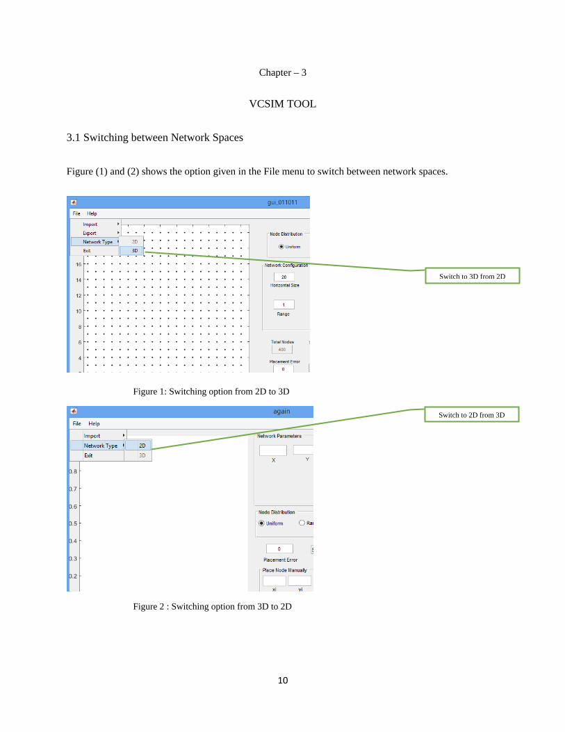
Figure (1) and (2) shows the option given in the File menu to switch between network spaces.

Figure 1: Switching option from 2D to 3D

Figure 2 : Switching option from 3D to 2D

Switch to 3D from 2D

Switch to 2D from 3D

11

3.2 GUI for Analysis

3.2.1 2D Routing

Figure 3 : GUI for 2D network space

Figure (3) shows the GUI for routing analysis and results for a 2D wireless sensor network. The routing

analysis method can be either exhaustive or random. The routing mechanisms are included under the

Method dropdown. Time to Live (TTL) is given in terms of route hops and the default value is 20. Routing

will be done until the route hops exceeds the TTL value and then the packet is dropped. A TTL value of 0

indicates that the routing should be done until the destination is reached without dropping the packet. Once

all the paths are simulated, the ‘Results’ button is enabled. A simulation can also be stopped before

completion by using the ‘Cancel’ option in the progress bar that will be displayed while the simulation is

underway.

12

3.2.2. 3D Routing

Figure (4) shows the GUI for routing analysis and results for a 3D wireless sensor network. The options for

analysis are similar to that of 2D but the routing mechanisms differ.

Figure 4 : GUI for 3D network space

3.2.3. Exhaustive Routing Analysis

Exhaustive Routing analysis calculates the path from each node to every other node. So in case of a network

with 150 nodes, 22350 routing simulations will be done. This is used to determine if all nodes are

approachable from every nodes in the network with a specified number of hops.

13

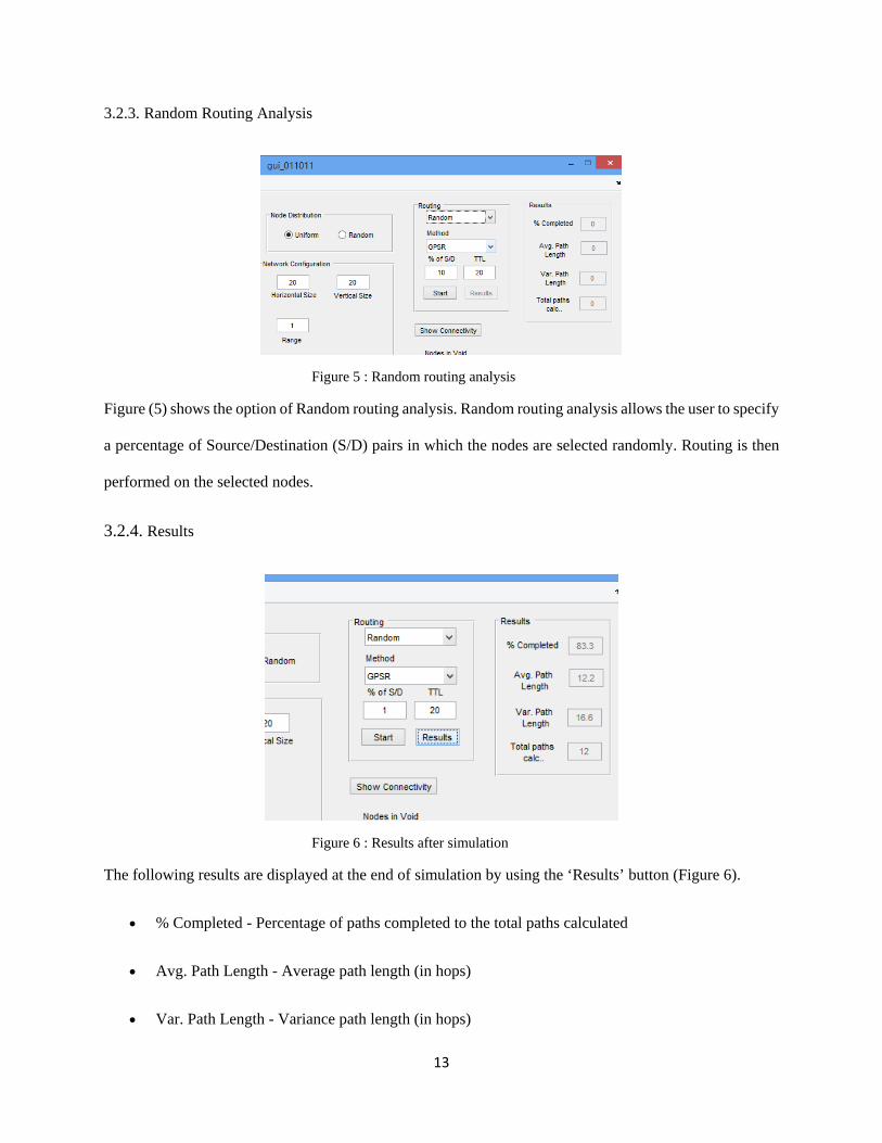
3.2.3. Random Routing Analysis

Figure 5 : Random routing analysis

Figure (5) shows the option of Random routing analysis. Random routing analysis allows the user to specify

a percentage of Source/Destination (S/D) pairs in which the nodes are selected randomly. Routing is then

performed on the selected nodes.

3.2.4. Results

Figure 6 : Results after simulation

The following results are displayed at the end of simulation by using the ‘Results’ button (Figure 6).

• % Completed - Percentage of paths completed to the total paths calculated

• Avg. Path Length - Average path length (in hops)

• Var. Path Length - Variance path length (in hops)

14

• Total paths calc. - Total number of paths calculated

• Histogram of hops against the number of nodes (shown in Figure (7))

Figure 7 : Histogram of hops

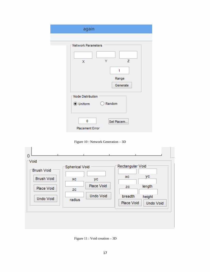
3.2.5. Generation of Topologies

The size of the network to be simulated must be specified by the user. Node placement could either be

'Uniform' or 'Random'. In 'Random' placement user must specify the node density in a given area assuming

each node is placed unit distance apart. Voids stand for the obstacles or absence of nodes in real

environment. User can also import the topologies by providing nodes [x, y] coordinates or whole network

15

as matrix. Place Node allows user to individually place each node. Void creation could be accomplished in

the following ways:

• 2D Network

1. Linear - Vertices of polygon shaped obstacles must be given by user. The vertices are joined

by a straight line to form a closed shape void.

2. Interpolation - Approximate vertices are given to form the interpolated closed shape.

3. Rectangle - Rectangular shaped polygons could be easily created.

4. Circle - It is easy to create elliptical shape voids with this option.

Figure 8 : Network generation – 2D

16

• 3D Network

1. Brush - Draw a void in the network of your own

2. Spherical - Create a spherical void by specifying the center and radius

3. Rectangular - Create a rectangular void by specifying one vertex and dimensions of the

rectangle

'Placement Tolerance' specifies the placement tolerance allowed for each node. 10% placement tolerance

mean nodes are placed within circle of 0.1 unit distance radius.

Figure 9 : Void creation – 2D

17

Figure 10 : Network Generation – 3D

Figure 11 : Void creation – 3D

18

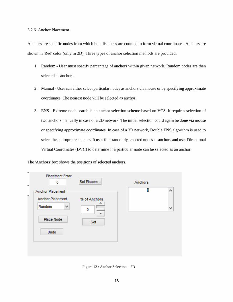
3.2.6. Anchor Placement

Anchors are specific nodes from which hop distances are counted to form virtual coordinates. Anchors are

shown in 'Red' color (only in 2D). Three types of anchor selection methods are provided:

1. Random - User must specify percentage of anchors within given network. Random nodes are then

selected as anchors.

2. Manual - User can either select particular nodes as anchors via mouse or by specifying approximate

coordinates. The nearest node will be selected as anchor.

3. ENS - Extreme node search is an anchor selection scheme based on VCS. It requires selection of

two anchors manually in case of a 2D network. The initial selection could again be done via mouse

or specifying approximate coordinates. In case of a 3D network, Double ENS algorithm is used to

select the appropriate anchors. It uses four randomly selected nodes as anchors and uses Directional

Virtual Coordinates (DVC) to determine if a particular node can be selected as an anchor.

The 'Anchors' box shows the positions of selected anchors.

Figure 12 : Anchor Selection – 2D

19

Figure 13 : Anchor Selection – 3D

3.2.7. Import Network

'Import' option under File menu enables user to import different network shapes and sizes. The 'Location'

option requires the physical coordinates [(x,y) for 2D and (x,y,z) for 3D] of the sensors to be given as an

input in a .mat file. The 'Network' option requires .mat file with a multi-dimensional array of 0s' and 1s'

where 1s' represent the node being present in the network and 0s' represent the absence of nodes at the

particular position.

20

Figure 14 : Import Network

3.2.8. Prospective Work

The current tool can be used to create network of desired size, shape and density in 2 and 3-D network

space, the tool also facilitates in choosing the anchors and calculating the Virtual Coordinates. Also it

enables to perform simulations using various routing mechanisms that are available. Furthermore, routing

algorithms can be added to the tool and the efficiency of those techniques can be calculated with ease.

21

REFERENCES

D. C. Dhanapala and A. P. Jayasumana, “Geo-logical routing in wireless sensor networks,” Proc. 8th Annual IEEE Communications Society Conference on Sensor, Mesh and Ad Hoc Communications and Networks (SECON), June 2011.

D. C. Dhanapala and A. P. Jayasumana, "Topology preserving maps from virtual coordinates for wireless sensor networks," Proc. 35th IEEE Conf. on Local Computer Networks, Oct. 2010.

Yi Jiang and A. P. Jayasumana, "Anchor Selection and Geo-Logical Routing in 3D Wireless Sensor Networks," Proc. 9th IEEE Local Computer Networking Conference, Edmonton, Canada, Sept. 2014.

Brad Karp and H. T. Kung. 2000. GPSR: greedy perimeter stateless routing for wireless networks. In Proceedings of the 6th annual international conference on Mobile computing and networking (MobiCom '00). ACM, New York, NY, USA, 243-254

Jiangwei Zhou, Yu Chen, Ben Leong, and Pratibha Sundar Sundaramoorthy. "Practical 3D Geographic Routing for Wireless Sensor Networks". Proceedings of the 8th ACM Conference on Embedded Networked Sensor Systems (SenSys 2010). Zurich, Switzerland. November 2010.