Embed Size (px)
Citation preview
PROJECT REPORT
Vo Thanh Huan

Contents
1 Preliminaries 51.1 Inner Product Spaces . . . . . . . . . . . . . . . . . . . . . . . . . . . . . . 5
1.1.1 Inner Product . . . . . . . . . . . . . . . . . . . . . . . . . . . . . . 51.1.2 Norm . . . . . . . . . . . . . . . . . . . . . . . . . . . . . . . . . . . 51.1.3 Gram-Schmidt Procedure . . . . . . . . . . . . . . . . . . . . . . . 71.1.4 Orthogonal Projections . . . . . . . . . . . . . . . . . . . . . . . . . 9
1.2 Linear Functionals and Adjoints . . . . . . . . . . . . . . . . . . . . . . . 91.2.1 The Adjoint of an Operator . . . . . . . . . . . . . . . . . . . . . . 91.2.2 Self-adjoint Operators . . . . . . . . . . . . . . . . . . . . . . . . . 121.2.3 The Spectral Theorem . . . . . . . . . . . . . . . . . . . . . . . . . 141.2.4 Positive Operators . . . . . . . . . . . . . . . . . . . . . . . . . . . 151.2.5 Functions of Self-adjoint Operators . . . . . . . . . . . . . . . . . . 16
1.3 Norms of Operators . . . . . . . . . . . . . . . . . . . . . . . . . . . . . . . 181.3.1 Bounded Linear Opearators . . . . . . . . . . . . . . . . . . . . . . 181.3.2 The Operator Norm . . . . . . . . . . . . . . . . . . . . . . . . . . 201.3.3 The Operator Norm of Self-Adjoint Operators . . . . . . . . . . . 231.3.4 Convergence of Matrices . . . . . . . . . . . . . . . . . . . . . . . . 24
1.4 Legendre Polynomials . . . . . . . . . . . . . . . . . . . . . . . . . . . . . 28
2 A Simple Case of the Atiyah–Singer Index Theorem 352.1 Introduction . . . . . . . . . . . . . . . . . . . . . . . . . . . . . . . . . . . 352.2 Gauge Fields . . . . . . . . . . . . . . . . . . . . . . . . . . . . . . . . . . . 382.3 Gauge Transformations . . . . . . . . . . . . . . . . . . . . . . . . . . . . . 412.4 Topological Charge . . . . . . . . . . . . . . . . . . . . . . . . . . . . . . . 422.5 Dirac Operators . . . . . . . . . . . . . . . . . . . . . . . . . . . . . . . . . 422.6 Chirality . . . . . . . . . . . . . . . . . . . . . . . . . . . . . . . . . . . . . 452.7 The Atiyah–Singer Index Theorem . . . . . . . . . . . . . . . . . . . . . . 48
3 Discretization of the Atiyah–Singer Index Theorem 523.1 Motivations . . . . . . . . . . . . . . . . . . . . . . . . . . . . . . . . . . . 523.2 Lattice Gauge Fields . . . . . . . . . . . . . . . . . . . . . . . . . . . . . . 523.3 Relation to Smooth Gauge Fields . . . . . . . . . . . . . . . . . . . . . . . 553.4 Gauge Transformations on the Lattice . . . . . . . . . . . . . . . . . . . . 573.5 Naive Index . . . . . . . . . . . . . . . . . . . . . . . . . . . . . . . . . . . 583.6 Spectral Flow . . . . . . . . . . . . . . . . . . . . . . . . . . . . . . . . . . 613.7 Hermitian Wilson-Dirac Operator . . . . . . . . . . . . . . . . . . . . . . . 66
3
Contents
3.8 Approximate Smoothness Condition . . . . . . . . . . . . . . . . . . . . . 703.9 Discrete Topological Charge . . . . . . . . . . . . . . . . . . . . . . . . . . 793.10 The Main Problem . . . . . . . . . . . . . . . . . . . . . . . . . . . . . . . 82
3.10.1 Piecewise Smooth Gauge Fields from Lattice Gauge Fields . . . . 843.10.2 Deformations of Lattice Gauge Fields . . . . . . . . . . . . . . . . 883.10.3 Index Density . . . . . . . . . . . . . . . . . . . . . . . . . . . . . . 913.10.4 Computational Approaches . . . . . . . . . . . . . . . . . . . . . . 92
Bibliography 95
4
1 Preliminaries
1.1 Inner Product Spaces
This chapter provides a brief overview of knowledge needed for subsequent chapters.Most of the materials are taken from [5].
1.1.1 Inner Product
Let V be a finite-dimensional vector space over a field F, where F denotes R or C. Aninner product on V is a function that takes each ordered pair (u, v) of elements of V to anumber 〈u, v〉 in F and satisfies the following properties:
1. 〈v, v〉 ≥ 0 for all v ∈ V ;
2. 〈v, v〉 = 0 if and only if v = 0;
3. 〈u+ v, w〉 = 〈u,w〉+ 〈v, w〉 for all u, v, w ∈ V ;
4. 〈av, w〉 = a 〈v, w〉 for all a ∈ F and v, w ∈ V ;
5. 〈v, w〉 = 〈w, v〉 for all v, w ∈ V .
Conditions 3 and 4 can be combined into the requirement of linearity in the first slot.Thus an inner product is linear in the first slot and conjugate linear in the second slot,i.e.,
〈u, v + w〉 = 〈u, v〉+ 〈u,w〉 and 〈u, aw〉 = a 〈u,w〉 .
Note that in the physics literature people often adopt the condition of linearity in thesecond slot and conjugate linearity in the first slot.
1.1.2 Norm
Let V be a nonzero finite-dimensional vector space. A norm on V is a function ‖·‖ : V →R satisfying the following properties
1. ‖v‖ ≥ 0 for v ∈ V ,
2. ‖v‖ = 0 if and only if v = 0,
3. ‖v + w‖ ≤ ‖v‖+ ‖w‖ for v, w ∈ V (triangle inequality),
4. ‖αv‖ = |α|‖v‖ for α ∈ C, v ∈ V .
5
1 Preliminaries
A vector space equipped with a norm is called a normed vector space. Given a normedvector space V , we can put a metric on V by
d(v, w) = ‖v − w‖, v, w ∈ V.
It’s easy to verify that all the properties of a metric are satisfied. In particular,
d(v, w) = ‖v − w‖ = ‖ − (w − v)‖ = | − 1|‖w − v‖ = d(w, v).
Given an inner product on V , we can define a norm on V as follows
‖v‖ =√〈v, v〉, v ∈ V.
Properties (1), (2), (4) of a norm follow directly from properties of an inner product. Wecheck the triangle inequality:
‖v + w‖2 = 〈v + w, v + w〉 = 〈v, v〉+ 〈v, w〉+ 〈w, v〉+ 〈w,w〉= ‖v‖2 + 〈v, w〉+ 〈v, w〉+ ‖w‖2
≤ ‖v‖2 + 2| 〈v, w〉 |+ ‖w‖2 ≤ ‖v‖2 + 2‖v‖‖w‖+ ‖w‖2
= (‖v‖+ ‖w‖)2 ,
where the last inequality follows from the Cauchy–Schwarz inequality:
| 〈v, w〉 | ≤ ‖v‖‖w‖,
which is true in any inner-product space. So every inner product induces a norm on avector space. However, not every norm arises from an inner product. The most familiarnorm on Rn is the Euclidean norm, given by
‖v‖ =
√√√√ n∑i=1
v2i for all v ∈ Rn.
It’s easily seen that the Euclidean norm arises from the usual inner product on Rn:
〈v, w〉 =
n∑i=1
viwi for all v, w ∈ Rn.
Another important norm on Rn is known as the sup norm, which is defined as
‖v‖sup = max {|v1|, |v2|, ..., |vn|} .
Note that since
|vi| ≤
√√√√ n∑i=1
v2i ≤√nmax {|v1|, ..., |vn|} ,
6
1.1 Inner Product Spaces
the relationship between the sup norm and the Euclidean norm is given by
‖v‖sup ≤ ‖v‖ ≤√n‖v‖sup.
The sup norm on R2 does not arise from any inner product on R2. If it did, then thefollowing identity
‖u+ v‖2sup + ‖u− v‖2sup = 2(‖v‖2sup + ‖w‖2sup
)for all v, w ∈ R2,
known as the parallelogram law would hold (this can be verified simply by expandingthe left hand side using the definition of norm induced from inner product). In the casewhere u = (1, 0)T and v = (0, 1)T , it’s easily seen that the above equality breaks down.Thus not every norm on V arises from an inner product on V .
1.1.3 Gram-Schmidt Procedure
Let v be a nonzero vector in V . For any vector u ∈ V , we’d like to write u as a sum of ascalar multiple of v and a vector orthogonal to v. Suppose
u = av + (u− av) for some scalar a ∈ F.
We want to choose a in such a way that
0 = 〈u− av, v〉 = 〈u, v〉 − a 〈v, v〉 = 〈u, v〉 − a‖v‖2.
Since v 6= 0, we obtain
a =〈u, v〉‖v‖2
.
Thus
u =〈u, v〉‖v‖2
v + w,
where w is orthogonal to v. The vector
〈u, v〉‖v‖2
v
is called the orthogonal projection of u onto v. Recall that a list of vectors (v1, ..., vn) isorthonormal if
〈vi, vj〉 = δij for 1 ≤ i, j ≤ n.
The Gram-Schmidt procedure allows us to turn an independent list of vectors to an or-thonormal list. More precisely,
Theorem 1.1 (Gram-Schmidt). If (v1, ..., vm) is an independent list of vectors, then thereexists an orthonormal list of vectors (e1, ..., em) such that
span(v1, ..., vj) = span(e1, ..., ej)
for j = 1, ...,m.
7
1 Preliminaries
We sketch the construction below. First we construct an orthogonal list, and then turnit into an orthonormal list by the normalization v/‖v‖. Put e1 = v1 and
e2 = v2 −〈v2, e1〉‖e1‖2
e1.
Generally,
ej = vj −〈vj , e1〉‖e1‖2
e1 − · · · −〈vj , ej−1〉‖ej−1‖2
ej−1,
for 1 < j ≤ m. In other words, to obtain ej , we subtract off from vj its projection ontothe subspace spanned by (e1, ..., ej−1). It can be shown that (e1, ..., em) is orthogonaland
span(v1, ..., vj) = span(e1, ..., ej)
for j = 1, ...,m. Thus every finite-dimensional inner-product space has an orthonormalbasis. One important corollary of the Gram-Schmidt procedure is the following
Corollary 1.1. Every orthonormal list of vectors can be extended to an orthonormal basis of V .
To see why, suppose (e1, ..., em) is an orthonormal list of vectors. Then it is indepen-dent and can be extended to a basis of V , say
(e1, ..., em, v1, ...., vn).
Apply the Gram-Schmidt procedure to the above list of vectors, we obtain an orthonor-mal basis of V . However, since the the first m vectors are orthonormal, they remain thesame after the procedure. We’ve extended (e1, ..., em) to an orthonormal basis of V .
One of the reasons orthonormal bases are useful is because the elements of V can beexpressed in a simple form. If (e1, ..., en) is an orthonormal basis for V and v ∈ V , then
v = a1e1 + · · ·+ anen for some scalars a1, ..., an ∈ F.
Now since (e1, ..., en) is orthonormal,
〈v, ej〉 =
⟨n∑i=1
aiei, ej
⟩=
n∑i=1
ai 〈ei, ej〉 = aj
for j = 1, ..., n. Thusv = 〈v, e1〉 e1 + · · ·+ 〈v, en〉 en.
We can also obtain the norm of v:
‖v‖2 = 〈v, v〉 =
⟨n∑i=1
〈v, ei〉 ei,n∑j=1
〈v, ej〉 ej
⟩=
n∑i=1
| 〈v, ei〉 |2.
8
1.2 Linear Functionals and Adjoints
1.1.4 Orthogonal Projections
If U is a subset of V , recall that the orthogonal complement of U , denoted by U⊥ is
U⊥ = {v ∈ V : 〈v, u〉 = 0 for all u ∈ U} .
The next theorem shows that every subspace of an inner-product space leads to a natu-ral direct sum decomposition of the whole space.
Theorem 1.2. If U is a subspace of V , then
V = U ⊕ U⊥.
Proof. First we show that every element v of V can be written as
v = u+ w,
where u ∈ U and w ∈ U⊥. Let (u1, ..., um) be an orthonormal basis for U and put
u = 〈v, u1〉u1 + 〈v, u2〉u2 + · · ·+ 〈v, um〉um.
Then clearly u ∈ U . Now we write v as
v = u+ (v − u).
We need to show that v − u ∈ U⊥. Indeed,
〈v − u, uj〉 = 〈v, uj〉 − 〈u, uj〉 = 〈v, uj〉 − 〈v, uj〉 = 0
for j = 1, ...,m. Thus v − u is orthogonal to each element in a basis of U and so it isorthogonal to every element of U .
Now take z ∈ U ∩ U⊥, then〈z, z〉 = 0.
Hence z = 0 and the intersection of U and U⊥ is trivial.
1.2 Linear Functionals and Adjoints
1.2.1 The Adjoint of an Operator
Recall that a linear functional on V is a linear map from V to the scalar F. For instance,if w is any element of V , the map ϕ : V → F given by
ϕ(v) = 〈v, w〉 for all v ∈ V
is a linear functional due to properties of the inner product. Interestingly, it turns outthat every linear functional is of this form.
9
1 Preliminaries
Theorem 1.3. Suppose ϕ is a linear functional on V . Then there is a unique v ∈ V such that
ϕ(u) = 〈u, v〉
for every u ∈ V .
Proof. We first show the existence of v. Let (e1, ..., en) be an orthonormal basis for V .For any u ∈ V , it can be written as
u = 〈u, e1〉 e1 + · · ·+ 〈u, en〉 en.
Thus
ϕ(u) = ϕ (〈u, e1〉 e1 + · · ·+ 〈u, en〉 en)
= 〈u, e1〉ϕ(e1) + · · ·+ 〈u, en〉ϕ(en) (by linearity of ϕ)
=⟨u, ϕ(e1)e1 + · · ·+ ϕ(en)en
⟩(because ϕ(ei) ∈ F) .
So v can be chosen asv = ϕ(e1)e1 + · · ·+ ϕ(en)en.
For the uniqueness of v, assume that
〈u, v1〉 = 〈u, v2〉 for all u ∈ V .
Then〈u, v1 − v2〉 = 0 for all u ∈ V .
Choose u to be v1 − v2, we obtain ‖v1 − v2‖ = 0. Therefore, v1 = v2.
We are now ready to define the adjoint of an operator. Let W be a finite-dimensionalinner-product space and T : V → W be a linear map. The adjoint of T , denoted by T ∗
is a linear map W → V and is defined as follows. For any w ∈ W , the map ϕ : V → Fgiven by
ϕ(u) = 〈T (u), w〉 for all u ∈ V
is a linear functional on V since T is linear (note that here we use the inner product onW ). Thus there exists a unique v ∈ V such that
ϕ(u) = 〈T (u), w〉 = 〈u, v〉 for all u ∈ V .
We define T ∗(w) = v. The above equality can be written as
〈T (u), w〉 = 〈u, T ∗(w)〉 for all u ∈ V and w ∈W.
We should check that T ∗ is linear. Indeed, for any u ∈ V and w1, w2 ∈W ,
〈u, T ∗(w1 + w2)〉 = 〈T (u), w1 + w2〉 = 〈T (u), w1〉+ 〈T (u), w2〉= 〈u, T ∗(w1)〉+ 〈u, T ∗(w2)〉 = 〈u, T ∗(w1) + T ∗(w2)〉 .
10
1.2 Linear Functionals and Adjoints
We conclude that T ∗(w1 + w2) = T ∗(w1) + T ∗(w2). Similarly, for any a ∈ F,
〈u, T ∗(aw)〉 = 〈T (u), aw〉 = a 〈T (u), w〉= a 〈u, T ∗(w)〉 = 〈u, aT ∗(w)〉 .
We conclude that T ∗(aw) = aT ∗(w). Thus T ∗ is linear.Let’s try to find the adjoint of a simple operator. Define T : R3 → R2 by
T (x1, x2, x3) = (x2 + 3x3, 2x1)
To find the adjoint, consider for any (y1, y2) ∈ R2
〈T (x1, x2, x3), (y1, y2)〉 = 〈(x2 + 3x3, 2x1), (y1, y2)〉 = x2y1 + 2x1y2 + 3x3y1
= 〈(x1, x2, x3), (2y2, y1, 3y1)〉 .
ThusT ∗(y1, y2) = (2y2, y1, 3y1).
We list some simple properties of the adjoint
Proposition 1.1. The function T 7→ T ∗ satisfies
1. (S + T )∗ = S∗ + T ∗ (additivity);
2. (aT )∗ = aT ∗ for a ∈ F (conjugate homogeneity);
3. (T ∗)∗ = T (adjoint of adjoint);
4. I∗ = I (identity)
5. (ST )∗ = T ∗S∗ (product).
Proof. These properties follow from the definition of the adjoint. For instance, property3 holds because
〈x, (T ∗)∗y〉 = 〈T ∗x, y〉 = 〈y, T ∗x〉 = 〈Ty, x〉 = 〈x, Ty〉 .
And for property 5, note that
〈x, (ST )∗y〉 = 〈STx, y〉 = 〈Tx, S∗y〉 = 〈x, T ∗(S∗y)〉 .
Recall that the conjugate transpose of a matrix A, denoted by A∗ is the matrix ob-tained from A by first taking the transpose and then take the conjugation of each entry.In symbols,
(A∗)ij = Aji, for all i, j.
The notation is no coincidence. We’ll show that the matrix representation of the adjointof an operator with respect to some orthonormal bases is the conjugate transpose ofthat of the operator.
11
1 Preliminaries
Proposition 1.2. Suppose T : V → W is a linear map. If (e1, ..., en) is an orthonormal basisfor V and (f1, ..., fm) is an orthonormal basis for W , then
M(T ∗, (f1, ..., fm), (e1, ..., en))
is the conjugate transpose of
M(T, (e1, ..., en), (f1, ..., fm)).
Proof. To avoid cumbersome notations, we’ll use M(T ∗) and M(T ). The bases are clearfrom context. Note that the (i, j)-entry of M(T ) is given by
(M(T ))ij = 〈T (ej), fi〉 = 〈ej , T ∗(fi)〉 = 〈T ∗(fi), ej〉 = (M(T ∗))ji,
where the first and last equalities follow from the orthonormality of the bases and thesecond equality follows from the definition of adjoint. By definition of conjugate trans-pose,
M(T )∗ = M(T ∗).
1.2.2 Self-adjoint Operators
An operator T on some finite-dimensional inner-product space is called self-adjoint orHermitian if T ∗ = T . From properties of the adjoint, it follows that the sum of twoself-adjoint operators is self-adjoint and the product of a real scalar and a self-adjointoperator is self-adjoint. Self-adjoint operators have several nice properties which we’regoing to illustrate below.
Proposition 1.3. Every eigenvalue of a self-adjoint operator is real.
Proof. Suppose T is a self-adjoint operator on V and λ is an eigenvalue of T . Then thereexists some nonzero vector v ∈ V such that T (v) = λv. We have
λ‖v‖2 = λ 〈v, v〉 = 〈λv, v〉 = 〈T (v), v〉 = 〈v, T ∗v〉= 〈v, T (v)〉 = 〈v, λv〉 = λ 〈v, v〉 = λ‖v‖2.
We conclude that λ = λ. Thus λ is real.
The next result is only true for complex inner-product spaces.
Proposition 1.4. If V is a complex inner-product space and T is an operator on V such that
〈Tv, v〉 = 0
for all v ∈ V , then T = 0.
This property is not true for real inner-product space. Consider the rotation of R2 byπ/2 counterclockwise. Clearly, 〈Tv, v〉 = 0, but T 6= 0.
12
1.2 Linear Functionals and Adjoints
Proof. The key is the following equality
〈Tu,w〉 =〈T (u+ w), u+ w〉 − 〈T (u− w), u− w〉
4
+〈T (u+ iw), u+ iw〉 − 〈T (u− iw), u− iw〉
4i,
which can be verified by expanding the right hand side. Since 〈Tv, v〉 = 0 for all v ∈ V ,we conclude that 〈Tu,w〉 = 0 for all u.w ∈ V . In particular, 〈Tu, Tu〉 = 0 for all u ∈ V ,which implies that T = 0.
One important corollary of the above proposition is the following.
Corollary 1.2. Let V be a complex inner-product space and T be a linear operator on V . ThenT is self-adjoint if and only if
〈Tv, v〉 ∈ R
for every v ∈ V .
Proof. Let v ∈ V . Then
〈Tv, v〉 − 〈Tv, v〉 = 〈Tv, v〉 − 〈v, Tv〉= 〈Tv, v〉 − 〈T ∗v, v〉= 〈(T − T ∗)v, v〉 .
Thus the condition 〈Tv, v〉 ∈ R for all v ∈ V is equivalent to 〈(T − T ∗)v, v〉 = 0 forall v ∈ V . Since we are over the complex field, the latter condition is equivalent toT − T ∗ = 0 by Proposition 1.4, i.e., T = T ∗.
We remark that an n × n matrix A can be thought of as an operator Cn → Cn in theusual manner. The (i, j)-entry of A is given by
Aij = 〈Aej , ei〉 ,
where ei is a standard basis element for Cn and the (j, i)-entry of A∗, the conjugatetranspose of A is given by
A∗ji = 〈A∗ei, ej〉 = Aij = 〈ei, Aej〉 .
Thus if A∗ = A, we have
〈Aei, ej〉 = 〈ei, Aej〉 for all i, j.
By properties of inner product,
〈Av,w〉 = 〈v,Aw〉 for all v, w ∈ Cn.
Hence the matrix A is self-adjoint if and only if A∗ = A, as expected.
13
1 Preliminaries
1.2.3 The Spectral Theorem
One of the nicest properties of complex self-adjoint operators is there exists an orthonor-mal basis for V consisting of eigenvectors of the operator. This result is known as thespectral theorem and it is our aim in this subsection to establish it. We record the theo-rem below.
Theorem 1.4 (Complex Spectral Theorem). Suppose that V is a complex inner-product spaceand T is an operator on V . Then T is self-adjoint if and only if V has an orthonormal basisconsisting of eigenvectors of T and all eigenvalues of T are real.
To prove the theorem, we need several lemmas. The most important one is
Lemma 1.1. Suppose V is a complex vector space and T is an operator on V . Then T has anupper-triangular matrix with respect to some basis of V .
Proof. We’re going to prove the result using induction on the dimension of V . The casewhere dimV = 1 is clearly true. So we assume that dimV > 1 and the lemma holdstrue for every complex vector space of dimension less than that of V and bigger than 0.
Let T be an operator on V . Since V is a complex vector space, T has an eigenvalueλ (the characteristic polynomial of T always has a solution). Consider the followingsubspace of V
U = range (T − λI).
Because λ is an eigenvalue of T , there exists some nonzero vector v ∈ V such that(T −λI)v = 0. Thus T −λI is not surjective and so dimU < dimV . Moreover, for everyu ∈ U , we can write
T (u) = (T − λI)u+ λu.
Clearly (T −λI)u ∈ U and λu ∈ U . Thus U is invariant under T . We can now apply theinduction hypothesis to (U, T |U ). Consequently there exists a basis (u1, ..., um) for Uwith respect to which T |U has an upper triangular matrix. Extend that basis to a basisfor V
(u1, ..., um, v1, ..., vn).
Now we haveT (ui) = T |U (ui) ∈ span(u1, ..., ui)
for i = 1, ...,m because the matrix of T |U is upper-triangular. For the vk, we can writeTvk as
T (vk) = (T − λI)vk + λvk
for k = 1, ..., n. Note that (T −λI)vk ∈ U and hence it belongs to the span of (u1, ..., um).We conclude that T (vk) ∈ span(u1, ..., um, v1, ..., vk) for k = 1, ..., n. We’ve found arequired basis.
The next lemma tells us that in fact we can choose the basis to be orthonormal.
Lemma 1.2. Suppose V is a complex vector space and T is an operator on V . Then T has anupper-triangular matrix with respect to some orthonormal basis of V .
14
1.2 Linear Functionals and Adjoints
Proof. We know that there exists a basis (v1, ..., vn) for V with respect to which T isupper-triangular. In other words, the subspaces (v1, ...vi) are invariant under T fori = 1, ..., n. Apply the Gram-Schmidt procedure to (v1, ..., vn) we obtain an orthonormalbasis (e1, ..., en) for V . Note that the procedure doesn’t change the span of the vectors,hence
span(v1, ..., vi) = span(e1, ..., ei) for i = 1, ..., n.
Thus span(e1, ..., ei) are also invariant under T for i = 1, ..., n, which implies that T isupper-triangular with respect to (e1, ..., en).
We are now ready to prove the complex spectral theorem. Suppose T is self-adjointand let (e1, ..., en) be an orthonormal basis for V such that M(T ) is upper-triangular(again we omit the basis, it is understood to be (e1, ..., en)). By orthonormality of(e1, ..., en), M(T ∗) is the conjugate transpose of M(T ), i.e.,
M(T ∗)ij = M(T )ji for 1 ≤ i, j ≤ n.
Since T is self-adjoint,
M(T )ij = M(T )ji for 1 ≤ i, j ≤ n.
Because T is upper-triangular, M(T )ij = 0 for n ≥ i > j ≥ 1. For i < j, the aboveequation implies that M(T )ij is also 0. Thus M(T ) is in fact diagonal and the basis(e1, ..., en) is an orthonormal basis for V consisting of eigenvectors of T .
For the other direction, suppose that V has an orthonormal basis (e1, ..., en) consistingof eigenvectors of T and that
T (ei) = λiei for i = 1, ..., n,
where λi ∈ R for i = 1, ..., n. For any v ∈ V , we have
v = a1e1 + · · ·+ anen for ai ∈ C.
Thus
〈Tv, v〉 =
⟨n∑i=1
aiTei,
n∑j=1
ajej
⟩=
⟨n∑i=1
aiλiei,
n∑j=1
ajej
⟩=
n∑i=1
|ai|2λi
by orthonormality of (e1, ..., en). Since all eigenvalues of T are real, we conclude that〈Tv, v〉 ∈ R for all v ∈ V . Hence T is self-adjoint by Corollary 1.2.
1.2.4 Positive Operators
Let T be an operator on some complex finite-dimensional inner-product space V . ThenT is called positive if
〈Tv, v〉 ≥ 0
15
1 Preliminaries
for all v ∈ V . For an example of a positive operator, take a nonzero vector v ∈ V andconsider the orthogonal projection onto v given by
Pv(u) =〈u, v〉‖v‖2
v for all u ∈ V .
We have
〈Pv(u), u〉 =
⟨〈u, v〉‖v‖2
v, u
⟩=| 〈u, v〉 |2
‖v‖2≥ 0.
Thus Pv is positive. Another important characteristic of positive operators is the fol-lowing.
Proposition 1.5. An operator T is positive if and only if it is self-adjoint and all of its eigen-values are non-negative.
Proof. Suppose that T is positive. Since V is a complex vector space, the condition〈Tv, v〉 ∈ R for all v ∈ V implies that T is self-adjoint. If λ is an eigenvalue of T witheigenvector v, then
0 ≤ 〈Tv, v〉 = λ 〈v, v〉 .
Thus λ ≥ 0 since 〈v, v〉 > 0.Now if T is self-adjoint and all the eigenvalues of T are non-negative. By the spectral
theorem, there exists an orthonormal basis (e1, ..., en) for V consisting of eigenvectorsof T . For any v ∈ V , we have
v = a1e1 + · · ·+ anen for ai ∈ C.
Thus
〈Tv, v〉 =
⟨n∑i=1
aiTei,
n∑j=1
ajej
⟩=
⟨n∑i=1
aiλiei,
n∑j=1
ajej
⟩=
n∑i=1
|ai|2λi
by orthonormality of (e1, ..., en). Since each eigenvalue λi is non-negative, we concludethat
〈Tv, v〉 ≥ 0
for all v ∈ V .
1.2.5 Functions of Self-adjoint Operators
One advantage of the spectral theorem is that it allows us to define operator-valuedfunctions of self-adjoint operators in terms of their eigenvalues. Let A be a self-adjointoperator on V and β = (v1, ..., vn) is an orthonormal basis for V consisting of eigenvec-tors of A, i.e.,
Avi = λivi, i = 1, ..., n.
16
1.2 Linear Functionals and Adjoints
If f is a complex-valued function that is defined on the eigenvalues ofA, then we definef(A) to be
f(A)vi = f(λi)vi, i = 1, ..., n.
and extend to the whole V using linearity. To have a good definition, we need to showthat it is independent of the choice of the orthonormal basis. Indeed, if w is an eigen-vector of A corresponding to an eigenvalue λ, then w can be expressed as a linear com-bination of independent eigenvectors
w =∑j
ajvj ,
where each vj ∈ β is an eigenvector of A corresponding to the eigenvalue λ. It followsthat
f(A)w =∑j
ajf(A)vj =∑j
ajf(λ)vj = f(λ)w.
Thus the definition of f(A) doesn’t depend on the choice of basis. From the definition,we also have
(f + g)(A) = f(A) + g(A),
(fg)(A) = f(A)g(A),
(f ◦ g)(A) = f(g(A)).
Note that our definition doesn’t account for every possible functions on operators. Forinstance, the following function
f(A) = PA
for some fixed matrix P is not obtained from any complex-valued function f . We giveseveral important examples of operator-valued functions.
1. If f is a polynomialf(z) = a0 + a1z + · · ·+ akz
k,
then f(A) is given by
f(A) = a0 + a1A+ · · ·+ akAk.
Note that the left hand side is defined in terms of the eigenvalues of A and theright hand side is the usual operations of operators. It’s easy to check that they’rein fact the same.
2. If f is given in term of a power series
f(z) =
∞∑k=0
akzk
17
1 Preliminaries
and the series converges on the eigenvalues of A, then we write f(A) as
f(A) =
∞∑k=0
akAk.
We’ll see later that this is just a special case of convergence of operators.
3. If A is a self-adjoint operator with non-zero eigenvalues, then
f(z) = z−1
is well-defined on the eigenvalues of A. The function
f(A)v = λ−1v
is the usual A−1.
4. If B is a self-adjoint operator with non-negative eigenvalues, i.e., a positive oper-ator, then
g(z) =√z
is well-defined on the eigenvalues of A (here we just consider the positive squareroot). The function
g(B)v =√λv
is known as the positive square root of B, which we denote by√B. Clearly,
(√B)2 = B,
as expected.
1.3 Norms of Operators
1.3.1 Bounded Linear Opearators
Let V and W be inner-product spaces. A linear map T : V → W is said to be bounded ifthere exists a real number c such that
‖T (v)‖ ≤ c‖v‖
for every v ∈ V . Note that here ‖T (v)‖ denotes the norm of T (v) in W . When there’sno ambiguity, we’ll use the same notation ‖ · ‖ to denote the norm. Note that the con-cept of boundedness here only applies to linear maps and it is different from the usualdefinition of boundedness used in calculus. For instance, the map f : R → R given byf(x) = x is unbounded in the usual sense of calculus since its range is the whole of R.However, it is a bounded linear map since
‖f(x)‖ = ‖x‖ ≤ c‖x‖
for any real number c > 1. Bounded linear maps have a nice property, as given by thenext proposition.
18
1.3 Norms of Operators
Proposition 1.6. If T : V →W is a bounded linear map, then T is continuous.
Proof. Since T is bounded, there exists c > 0 such that
‖T (v)‖ ≤ c‖v‖, v ∈ V.
Let ε > 0 be arbitrary. For v, w ∈ V such that ‖v − w‖ < ε/c, we have
‖T (v)− T (w)‖ = ‖T (v − w)‖ ≤ c‖v − w‖ < ε,
where the first equality uses the linearity of T . Thus T is continuous.
The next proposition shows that linear maps between finite-dimensional inner-productspaces are continuous, as expected.
Lemma 1.3. Let T : V →W be a linear map between finite-dimensional inner-product spaces,then T is bounded.
Proof. Let {v1, ..., vn} be an orthonormal basis for V . For any v ∈ V , we have
v =n∑k=1
akvk, ak ∈ C.
Thus
‖v‖2 = 〈v, v〉 =
⟨n∑k=1
akvk,n∑l=1
alvl
⟩=
n∑k=1
|ak|2,
where the last equality follows from the orthonormality of {v1, ..., vn}. The Cauchy–Schwarz inequality now gives
n∑k=1
|ak|2 ≥1
n
(n∑k=1
|ak|
)2
.
Hence we obtain
‖v‖ ≥ 1√n
n∑k=1
|ak|.
Now
‖T (v)‖ =
∥∥∥∥∥n∑k=1
akT (vk)
∥∥∥∥∥ ≤n∑k=1
|ak|‖T (vk)‖ ≤ cn∑k=1
|ak|,
where c > 0 is the maximum value of {‖T (v1)‖, ..., ‖T (vk)‖}, independent of the vectorv. Therefore,
‖T (v)‖ ≤ cn∑k=1
|ak| ≤ c√n‖v‖
for any v ∈ V . So T is bounded.
19
1 Preliminaries
Recall that a subset K of a metric space M is compact if every open cover of K con-tains a finite subcover. Let V be an inner product space and {v1, ..., vn} be an orthonor-mal basis for V . The following map T : Cn → V given by
T (ek) = vk, k = 1, ..., n,
where {e1, ..., en} is the standard basis for Cn, is clearly an invertible linear map. Sincelinear maps are continuous, it is also an homeomorphism. Let x be any vector of Cnand suppose
x =
n∑k=1
akek, ak ∈ C,
then
‖T (x)‖2 =
⟨n∑k=1
akT (ek),n∑l=1
alT (el)
⟩=
⟨n∑k=1
akvk,n∑l=1
alvl
⟩
=n∑k=1
|ak|2 =
⟨n∑k=1
akek,n∑l=1
alel
⟩= ‖x‖2.
So T preserves the norm. Therefore, the subset
{v ∈ V : ‖v‖ = 1}
of V is the image of the subset
{x ∈ C : ‖x‖ = 1}
of Cn under T . Since the latter set is compact, we know that the former set is alsocompact.
1.3.2 The Operator Norm
Let T : V →W be a linear map between finite-dimensional inner-product spaces. Con-sider the following set
A =
{‖T (v)‖‖v‖
: v ∈ V and v 6= 0
}.
(A is nonempty because we assume that V is nonzero.) Since T is bounded, the set A isbounded above by some c > 0. The operator norm of T is defined to be
‖T‖ = supA.
The following inequality is immediate from the definition
‖T (v)‖ ≤ ‖T‖‖v‖ for all v ∈ V.
20
1.3 Norms of Operators
We check that ‖ · ‖ is indeed a norm on the space of linear maps V → W . Property(1) is trivial because each element of A is nonnegative. For property (2), if T = 0, thenA = {0}, thus ‖T‖ = 0. Conversely, if ‖T‖ = 0, then
‖T (v)‖ ≤ ‖T‖‖v‖ = 0 for all v ∈ V.
Thus T = 0. To show property (3), take any linear maps T and S and note that for anynonzero v ∈ V ,
‖(T + S)(v)‖ = ‖T (v) + S(v)‖ ≤ ‖T (v)‖+ ‖S(v)‖≤ ‖T‖‖v‖+ ‖S‖‖v‖ = (‖T‖+ ‖S‖)‖v‖.
Thus‖(T + S)(v)‖
‖v‖≤ ‖T‖+ ‖S‖
for any nonzero v ∈ V . It follows that
‖T + S‖ ≤ ‖T‖+ ‖S‖.
Finally, for any α ∈ C,
‖αT‖ = sup
{‖αT (v)‖‖v‖
: v ∈ V and v 6= 0
}= sup
{|α|‖T (v)‖
‖v‖: v ∈ V and v 6= 0
}= |α| sup
{‖T (v)‖‖v‖
: v ∈ V and v 6= 0
}= |α|‖T‖.
That shows property (4).It turns out that to find the operator norm, we don’t need to consider every v ∈ V , as
the next proposition shows.
Proposition 1.7. Let T : V → W be a linear map between finite-dimensional inner-productspaces. An alternative formula for the operator norm of T is
‖T‖ = sup{‖T (v)‖ : v ∈ V and ‖v‖ = 1}.
Proof. We let b denote the right hand side of the above expression. The subset consid-ered is clearly a subset of A (when ‖v‖ = 1), thus b ≤ ‖T‖. On the other hand, since Tis linear,
‖T (v)‖‖v‖
=
∥∥∥∥ 1
‖v‖T (v)
∥∥∥∥ =
∥∥∥∥T ( v
‖v‖
)∥∥∥∥ ≤ bfor every nonzero v ∈ V because the norm of v/‖v‖ is 1. Thus ‖T‖ ≤ b. We concludethat b = ‖T‖.
21
1 Preliminaries
Since {v ∈ V : ‖v‖ = 1} is compact, we can in fact replace supremum by maximum inthe formula for the operator norm. Some other useful properties of the operator normare given in the next proposition.
Proposition 1.8. Let T , S be operators on a finite-dimensional inner-product space V , then
1. ‖TS‖ ≤ ‖T‖‖S‖,
2. | 〈T (v), w〉 | ≤ ‖T‖‖v‖‖w‖ for all v, w ∈ V ,
3. ‖T‖ = ‖T ∗‖,
4. ‖TT ∗‖ = ‖T ∗T‖ = ‖T‖2.
Proof. To prove (1), note that
‖TS(v)‖ = ‖T (S(v))‖ ≤ ‖T‖‖S(v)‖ ≤ ‖T‖‖S‖‖v‖
for all v ∈ V . Thus ‖TS‖ ≤ ‖T‖‖S‖. For (2), we apply the Cauchy-Schwarz inequality
| 〈T (v), w〉 | ≤ ‖T (v)‖‖w‖ ≤ ‖T‖‖v‖‖w‖.
Property (3) is trivial for the case T = 0. Assume T 6= 0, we have
‖T (v)‖2 = 〈T (v), T (v)〉 = 〈T ∗Tv, v〉 ≤ ‖T ∗T‖‖v‖2
for any v ∈ V . Here the last inequality follows from property (2). Taking the squaredroot, we get
‖T (v)‖ ≤√‖T ∗T‖‖v‖ for any v ∈ V.
Thus by definition of the operator norm,
‖T‖ ≤√‖T ∗T‖.
Hence,‖T‖2 ≤ ‖T ∗T‖ ≤ ‖T ∗‖‖T‖,
where the last inequality uses property (1). Dividing both sides by ‖T‖ 6= 0 yields
‖T‖ ≤ ‖T ∗‖.
The same inequality applies to T ∗, thus
‖T ∗‖ ≤ ‖T ∗∗‖ = ‖T‖.
We conclude that ‖T‖ = ‖T ∗‖. Finally, since ‖T‖ = ‖T ∗‖,
‖T‖2 ≤ ‖T ∗T‖ ≤ ‖T ∗‖‖T‖ = ‖T‖2.
Thus ‖T‖2 = ‖T ∗T‖. Applying the same equality to T ∗ we obtain
‖T‖2 = ‖T ∗‖2 = ‖T ∗∗T ∗‖ = ‖TT ∗‖.
That completes the proof.
22

1.3 Norms of Operators
1.3.3 The Operator Norm of Self-Adjoint Operators
So far we haven’t given any examples of how to compute the operator norm. If T = 0,then ‖T‖ = 0. The simplest non-trivial example is the identity map T (v) = v forall v ∈ V . In which case, it’s easily seen that ‖T‖ = 1. For a general operator, it’snot a trivial matter to compute the operator norm directly from the definition. In thissubsection, we focus on finding the operator norm of self-adjoint operators. Our mainresult is the following.
Proposition 1.9. Let T be a self-adjoint operator on a finite-dimensional inner-product spaceV . Then
‖T‖ = max{|λ| : λ is an eigenvalue of T}.
Actually this proposition allows us to find the operator norm of every linear operatorT since we know that
‖TT ∗‖ = ‖T ∗T‖ = ‖T‖2
and the operator TT ∗ is self-adjoint.
Proof. The proof becomes quite straightforward once we know the spectral theorem.Let (e1, ..., en) be an orthonormal basis for V consisting of eigenvectors of T , i.e.,
Tei = λiei, i = 1, ..., n.
Then for any v ∈ V such that ‖v‖ = 1 we have
‖Tv‖2 =
∥∥∥∥∥T(
n∑i=1
〈v, ei〉 ei
)∥∥∥∥∥2
=
∥∥∥∥∥n∑i=1
〈v, ei〉Tei
∥∥∥∥∥2
=
∥∥∥∥∥n∑i=1
〈v, ei〉λiei
∥∥∥∥∥2
=n∑i=1
|〈v, ei〉λi|2
≤ maxi|λi|2
n∑i=1
| 〈v, ei〉 |2 = maxi|λi|2
and the equality occurs when v is one of (e1, ..., en). Thus
‖T‖ = sup {‖Tv‖ : ‖v‖ = 1} = maxi|λi|.
For an example, suppose we want to find the operator norm of the following self-adjoint operator C2 → C2
A =
(1 i−i 2
).
The characteristic polynomial of A is
λ2 − 3λ+ 1 = 0,
23
1 Preliminaries
which has solutions
λ =3±√
5
2.
Hence
‖A‖ =3 +√
5
2.
If we apply the definition directly, then we want to find the maximum of
2|u|2 + 5|v|2 + 3i(vu− uv),
where u and v are complex numbers subject to the condition |u|2 + |v|2 = 1, which isnot very easy.
The next proposition gives yet another formula for the operator norm of a self-adjointoperator.
Proposition 1.10. Let T be a self-adjoint operator on an inner-product space V . Then
‖T‖ = sup {| 〈Tv, v〉 | : ‖v‖ = 1} .
Proof. Since T is self-adjoint, we can choose an orthonormal basis for V consisting ofeigenvectors of T , i.e.,
Tei = λiei, i = 1, ..., n.
For any v ∈ V such that ‖v‖ = 1, we have
| 〈Tv, v〉 | =
∣∣∣∣∣∣⟨
n∑i=1
〈v, ei〉λiei,n∑j=1
〈v, ej〉 ej
⟩∣∣∣∣∣∣=
∣∣∣∣∣n∑i=1
λi| 〈v, ei〉 |2∣∣∣∣∣ ≤ max
i|λi|
and the equality happens when v is one of (e1, ..., en). Thus
sup {〈Tv, v〉 : ‖v‖ = 1} = maxi|λi| = ‖T‖.
1.3.4 Convergence of Matrices
Let V be a finite-dimensional inner-product space over C. The set of all operators on Vequipped with the operator norm is a metric space and thus we can talk about conver-gence of operators. Let (Bk) be a sequence of operators on V . If we choose an orthonor-mal basis (e1, ..., en) for V , then each Bk can be represented as an n× n complex matrixBk.
24
1.3 Norms of Operators
Proposition 1.11. The sequence (Bk) converges to some operatorA in the operator norm if andonly if
limk→∞
(Bk)ij = Aij
for 1 ≤ i, j ≤ n.
Proof. It suffices to prove the proposition in the case where A = 0, i.e.,
limk→∞
Bk = 0
in the operator norm if and only if
limk→∞
(Bk)ij = 0
for 1 ≤ i, j ≤ n. For the forward direction, suppose that
limk→∞
Bk = 0
in the operator norm, i.e., for every ε > 0, there exists some integer N such that
‖Bk‖ < ε for all k ≥ N.
Now since (e1, ..., en) is orthonormal, we have
|(Bk)ij | = | 〈Bkej , ei〉 | ≤ ‖Bkej‖‖ei‖ ≤ ‖Bk‖ < ε
for k ≥ N . Thereforelimk→∞
(Bk)ij = 0
for 1 ≤ i, j ≤ n.For the other direction, suppose that
limk→∞
(Bk)ij = 0
for 1 ≤ i, j ≤ n. Then for any ε > 0, there exists some integer N such that∑1≤i,j≤n
|(Bk)ij |2 < ε2 for all k ≥ N.
It follows that
‖Bkej‖2 =
n∑i=1
|(Bk)ij |2 < ε2 for all k ≥ N
for j = 1, ..., n. Now for every vector v ∈ V such that ‖v‖ = 1, we have
v =n∑j=1
ajej ,
25
1 Preliminaries
where |a1|2 + · · ·+ |an|2 = 1. Hence
‖Bkv‖2 = 〈Bkv,Bkv〉 =
n∑j=1
|aj |2‖Bkej‖2 < ε2
for k ≥ N . By the definition of the operator norm, we conclude that
‖Bk‖ < ε for all k ≥ N.
In other words,limk→∞
Bk = 0.
Thus if we have
A =
∞∑k=0
Bk,
then
A =∞∑k=0
Bk.
(Here the convergence of matrices means the convergence of each entry.) The trace ofA doesn’t depend on the choice of basis, hence
trA =n∑i=1
(A)ii =n∑i=1
∞∑k=0
(Bk)ii =∞∑k=0
n∑i=1
(Bk)ii =∞∑k=0
trBk.
We also note that if B is a self-adjoint operator such that
A =∞∑k=0
akBk,
consider an orthonormal basis for V consisting of eigenvectors of B, it follows fromTheorem 1.11 that the eigenvalues of A are given by{ ∞∑
k=0
akλk : λ is an eigenvalue of B
}.
This is in accordance with our definition of∑akB
k given in Subsection 1.2.5.
Proposition 1.12. The set of all operators on V equipped with the operator norm is a completemetric space, i.e., every Cauchy sequence converges.
26
1.3 Norms of Operators
Proof. Consider a Cauchy sequence (Bk), i.e., for every ε > 0, there exists some integerN such that
‖Bp −Bq‖ < ε for all p, q ≥ N.
Thus for j = 1, ..., n,
‖(Bp −Bq)ej‖ < ε for all p, q ≥ N.
It follows that|(Bp)ij − (Bq)ij | < ε for all p, q ≥ N
for 1 ≤ i, j ≤ n. Thus each sequence (Bk)ij is Cauchy. Since C is complete, we have
limk→∞
(Bk)ij = Aij .
By Proposition 1.11, we conclude that
limk→∞
Bk = A,
where A is the operator on V whose matrix representation with respect to (e1, ..., en) isA.
Proposition 1.13. If L is an operator on V such that ‖L‖ < 1, then
1
1− L=
∞∑k=0
Lk.
Note that L0 = I , the identity operator.
Proof. This proposition is an analogue of a result for complex numbers for the case ofoperators. It says that if ‖L‖ < 1, then 1 − L is invertible and can be represented by apower series of operators. To show the result, we first prove that the series on the righthand side is convergent and then show that its sum is precisely the inverse of 1−L. Forpositive integers q > p we have∥∥∥∥∥
q∑k=0
Lk −p∑
k=0
Lk
∥∥∥∥∥ =
∥∥∥∥∥∥q∑
k=p+1
Lk
∥∥∥∥∥∥ ≤q∑
k=p+1
∥∥∥Lk∥∥∥ ≤ q∑k=p+1
‖L‖k,
where the last inequality follows from a property of the operator norm. Because theseries
∞∑k=0
‖L‖k
is convergent for ‖L‖ < 1, we conclude that the sequence of partial sums of the se-ries
∑Lk form a Cauchy sequence. By Proposition 1.12, the series converges to some
operator S
S =
∞∑k=0
Lk.
27
1 Preliminaries
Multiply through both sides with L we obtain
LS =
∞∑k=1
Lk = S − I.
Thus
S = (I − L)−1 =1
1− L.
1.4 Legendre Polynomials
Consider the inner product space X consisting of all continuous real-valued functionson [−1, 1] with the inner product given by
〈x, y〉 =
∫ 1
−1x(t)y(t)dt.
(Note that X is an infinite-dimensional vector space.) We want to obtain an orthonor-mal sequence in X which consists of functions that are easy to handle. Polynomials areof this type and we start from the linearly independent sequence of powers:
x0(t) = 1, x1(t) = t, ..., xk(t) = tk, ... t ∈ [−1, 1].
Applying the Gram-Schmidt procedure (Theorem 1.1) we obtain an orthonormal se-quence (en). Each en is clearly a polynomial since it is just a linear combination of (xn)and we claim that (en) have the following explicit form:
en(t) =
√2n+ 1
2Pn(t) n = 0, 1, ..., (1.1)
where
Pn(t) =1
2nn!
dn
dtn[(t2 − 1)n].
The polynomial Pn is called the Legendre polynomial of order n and the formula for Pngiven above is known as the Rodrigues’ formula. The explicit form of the polynomialen may be found by applying the Gram-Schmidt procedure directly. However here wepresent another method. For this the following proposition is crucial.
Proposition 1.14. Let (yn) be an orthonormal sequence in X , where each yn is a polynomial ofdegree n for n = 0, 1, 2... Then we have
yn = ±en n = 0, 1, 2...
28
1.4 Legendre Polynomials
Proof. From the Gram-Schmidt procedure we have
Yn = span {x0, ..., xn} = span {e0, ..., en}
for all n. Then Yn is vector space of dimension n + 1. Since each yn is a polynomial ofdegree n, we conclude that
span {y0, ..., yn} ⊂ Yn.
Moreover, y0, ..., yn are linearly independent since they are orthogonal. Thus
Yn = span {y0, ..., yn} n = 0, 1, ...
It follows that we can express yn as a linear combination of en:
yn =n∑j=0
αjej , αj ∈ R.
Now by the orthogonality
yn ⊥ Yn−1 = span {y0, ..., yn−1} = span {e0, ..., en−1} ,
we obtain for k = 0, 1, ..., n− 1,
0 = 〈yn, ek〉 =
⟨n∑j=0
αjej , ek
⟩= αk.
Therefore,yn = αnen
for n = 0, 1, ... (The case n = 0 can be checked manually.) Since both yn and en are unitvectors, we have
1 = ‖yn‖ = |αn|‖en‖ = |αn|.
Because αn is real, αn is ±1.
In our case we can let yn to be the right hand side of (1.1). Then clearly each yn is apolynomial of degree n since Pn is a polynomial of degree 2n and we differentiate it ntimes. If (yn) is orthonormal, then
yn = ±enby Proposition 1.14. Furthermore, the coefficient of tn in en is positive (recall the for-mula of the Gram-Schmidt procedure) and so is the coefficient of tn in yn (the coefficientof t2n is positive). By equating the coefficients of tn in both polynomials we concludethat
yn = en
for n = 0, 1, 2... Thus now we just need to prove that the sequence (yn) is orthonormal.For that purpose the following observation is useful.
29
1 Preliminaries
Proposition 1.15. Put u(t) = t2 − 1. Then we have
(un)(k)(±1) = 0, k = 0, ..., n− 1
and(un)(2n) = (2n)!,
where (un)(k) denotes the k-th derivative of un.
Proof. We recall the general Leibniz rule for repeated differentiation:
(fg)(k) =k∑j=0
(k
j
)f (j)g(k−j),
which can be proved easily by induction. Applying this formula to un we obtain
dk
dtkun =
dk
dtk[(t− 1)n(t+ 1)n]
=
k∑j=0
(k
j
)[(t− 1)n](j)[(t+ 1)n](k−j)
=
k∑j=0
(k
j
)n · · · (n− j + 1)(t− 1)n−jn · · · (n− k + j + 1)(t+ 1)n−k+j .
Now for 0 ≤ k ≤ n − 1, both n − j and n − (k − j) are positive. Hence every termof (un)(k) contains the factor t2 − 1 and thus vanishes when t = ±1. For the secondequality, note that
(un)(2n) = (t2n)(2n) = (2n)!.
Proposition 1.16. The sequence (yn) is orthonormal.
Proof. Put u(t) = t2 − 1. Applying integration by parts n times we obtain
(2nn!)2‖Pn‖2 =
∫ 1
−1(un)(n)(un)(n)dt
= (un)(n−1)(un)(n)∣∣∣1−1−∫ 1
−1(un)(n+1)(un)(n−1)dt
= −(
(un)(n+1)(un)(n−2)∣∣∣1−1−∫ 1
−1(un)(n+2)(un)(n−2)dt
)= · · ·
= (−1)n−1
((un)(2n)(un)
∣∣∣1−1−∫ 1
−1(un)(2n)undt
)= (−1)n(2n)!
∫ 1
−1(t2 − 1)ndt
= 2(2n)!
∫ 1
0(1− t2)ndt,
30
1.4 Legendre Polynomials
where we’ve used (un)(k)(±1) = 0 for k = 0, ..., n− 1 and (un)(2n) = (2n)!. Now for theintegral
In =
∫ 1
0(1− t2)ndt,
by integration by parts we obtain the following recurrence relation
In =2n
2n+ 1In−1, n ≥ 1.
Since I0 = 1 we obtain
In =
(2n
2n+ 1
)(2n− 2
2n− 1
)· · · 2
3.
Plug in everything we get
(2nn!)2‖Pn‖2 =22n+1(n!)2
2n+ 1.
Thus‖Pn‖2 =
2
2n+ 1.
It follows that
‖yn‖2 =
∥∥∥∥∥√
2n+ 1
2Pn(t)
∥∥∥∥∥2
= 1.
Now for the orthogonality, we’ll show that 〈Pm, Pn〉 = 0 for 0 ≤ m < n. Since Pm is apolynomial, it suffices to prove that 〈xm, Pn〉 = 0 for 0 ≤ m < n. Applying integrationby parts m times we obtain
〈xm, Pn〉 =
∫ 1
−1tm(un)(n)dt
= tm(un)(n−1)∣∣∣1−1−∫ 1
−1mtm−1(un)(n−1)dt
= · · ·
= (−1)mm!
∫ 1
−1(un)(n−m)dt
= (−1)mm!(un)(n−m−1)∣∣∣1−1
= 0,
where the last equality follows because 0 ≤ m < n.
We can expand (t2 − 1)n using the binomial theorem:
(t2 − 1)n =n∑j=0
(n
j
)(t2)j(−1)n−j .
31
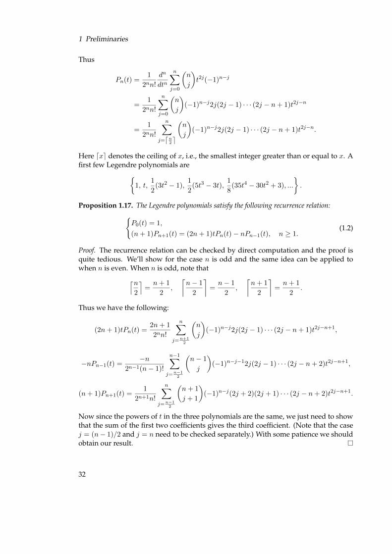
1 Preliminaries
Thus
Pn(t) =1
2nn!
dn
dtn
n∑j=0
(n
j
)t2j(−1)n−j
=1
2nn!
n∑j=0
(n
j
)(−1)n−j2j(2j − 1) · · · (2j − n+ 1)t2j−n
=1
2nn!
n∑j=dn2 e
(n
j
)(−1)n−j2j(2j − 1) · · · (2j − n+ 1)t2j−n.
Here dxe denotes the ceiling of x, i.e., the smallest integer greater than or equal to x. Afirst few Legendre polynomials are{
1, t,1
2(3t2 − 1),
1
2(5t3 − 3t),
1
8(35t4 − 30t2 + 3), ...
}.
Proposition 1.17. The Legendre polynomials satisfy the following recurrence relation:{P0(t) = 1,
(n+ 1)Pn+1(t) = (2n+ 1)tPn(t)− nPn−1(t), n ≥ 1.(1.2)
Proof. The recurrence relation can be checked by direct computation and the proof isquite tedious. We’ll show for the case n is odd and the same idea can be applied towhen n is even. When n is odd, note that⌈n
2
⌉=n+ 1
2,
⌈n− 1
2
⌉=n− 1
2,
⌈n+ 1
2
⌉=n+ 1
2.
Thus we have the following:
(2n+ 1)tPn(t) =2n+ 1
2nn!
n∑j=n+1
2
(n
j
)(−1)n−j2j(2j − 1) · · · (2j − n+ 1)t2j−n+1,
−nPn−1(t) =−n
2n−1(n− 1)!
n−1∑j=n−1
2
(n− 1
j
)(−1)n−j−12j(2j − 1) · · · (2j − n+ 2)t2j−n+1,
(n+ 1)Pn+1(t) =1
2n+1n!
n∑j=n−1
2
(n+ 1
j + 1
)(−1)n−j(2j + 2)(2j + 1) · · · (2j − n+ 2)t2j−n+1.
Now since the powers of t in the three polynomials are the same, we just need to showthat the sum of the first two coefficients gives the third coefficient. (Note that the casej = (n− 1)/2 and j = n need to be checked separately.) With some patience we shouldobtain our result.
32
1.4 Legendre Polynomials
Note that P0(t) = 1 for all t ∈ [−1, 1] and P1(1) = 1. Suppose that Pn−1(1) = Pn(1) =1, it follows from the recurrence relation that
(n+ 1)Pn+1(1) = (2n+ 1)− n = n+ 1.
Thus we have Pn(1) = 1 for n = 0, 1, 2, ... Moreover, it can be shown that |Pn(t)| ≤ 1 forall n. Hence for a fixed t ∈ [−1, 1], the following series
Qt(x) =
∞∑n=0
Pn(t)xn
is convergent for all x ∈ R and |x| < 1. We’d like to find the function Qt(x). First,differentiate Qt(x) with respect to x and multiply both sides by x we obtain
xQ′t(x) =∞∑n=1
nPn(t)xn, |x| < 1.
Using the recurrence relation (1.2) we obtain
xQ′t(x) = tx+∞∑n=1
(n+ 1)Pn+1(t)xn+1
= tx+
∞∑n=1
[(2n+ 1)tPn(t)− nPn−1(t)]xn+1
=∞∑n=1
2ntPn(t)xn+1 +∞∑n=1
tPn(t)xn+1 −∞∑n=1
nPn−1(t)xn+1 + tx
= 2tx2Q′t(x) + tx(Qt(x)− 1)− (x3Q′t(x) + x2Qt(x)) + tx
= (2tx2 − x3)Q′t(x) + (tx− x2)Qt(x)
Thus,(1− 2tx+ x2)Q′t(x) = (t− x)Qt(x), |x| < 1.
(Note that this holds for x = 0 because Qt(x) is continuous.) Now
1− 2tx+ x2 = (x− t)2 + (1− t2) > 0
because |t| ≤ 1 and |x| < 1. It follows that Qt(x) satisfies the initial value problemQ′t(x) =
(t− x
1− 2tx+ x2
)Qt(x),
Qt(0) = P0(t) = 1.
By separation of variables we get
Qt(x) =1√
x2 − 2tx+ 1.
33
1 Preliminaries
Therefore,1√
x2 − 2tx+ 1=∞∑n=0
Pn(t)xn, |x| < 1, |t| ≤ 1.
The function Qt(x) is called the generating function of the Legendre polynomials.From the generating function perspective, we can derive another important property
of the Legendre polynomials. We have
∞∑n=0
Pn(t)(−x)n = Qt(−x) =1√
x2 + 2tx+ 1= Q−t(x) =
∞∑n=0
Pn(−t)xn.
By uniqueness of power series expansion we conclude that
(−1)nPn(t) = Pn(−t).
Thus Pn is an odd polynomial if n is odd and is an even polynomial if n is even.
Proposition 1.18. The Legendre polynomial Pn satisfies the following differential equation:
(x2 − 1)y′′ + 2xy′ − n(n+ 1)y = 0,
or equivalently, [(x2 − 1)y′
]′ − n(n+ 1)y = 0.
Proof. Put u(x) = (x2 − 1)n, then u(n) = 2nn!Pn and
(x2 − 1)u′(x) = n2x(x2 − 1)n = 2nxu(x).
Differentiate the above equation n+ 1 times using the general Leibniz rule for repeateddifferentiation:
(fg)(k) =k∑j=0
(n
k
)f (k)g(n−k)
we obtain
n+1∑j=0
(n+ 1
j
)(x2 − 1)(j)(u′)(n+1−j) = 2n
n+1∑j=0
(n+ 1
j
)x(j)u(n+1−j)
Expand and combine the terms we get our desired differential equation.
34
2 A Simple Case of the Atiyah–SingerIndex Theorem
2.1 Introduction
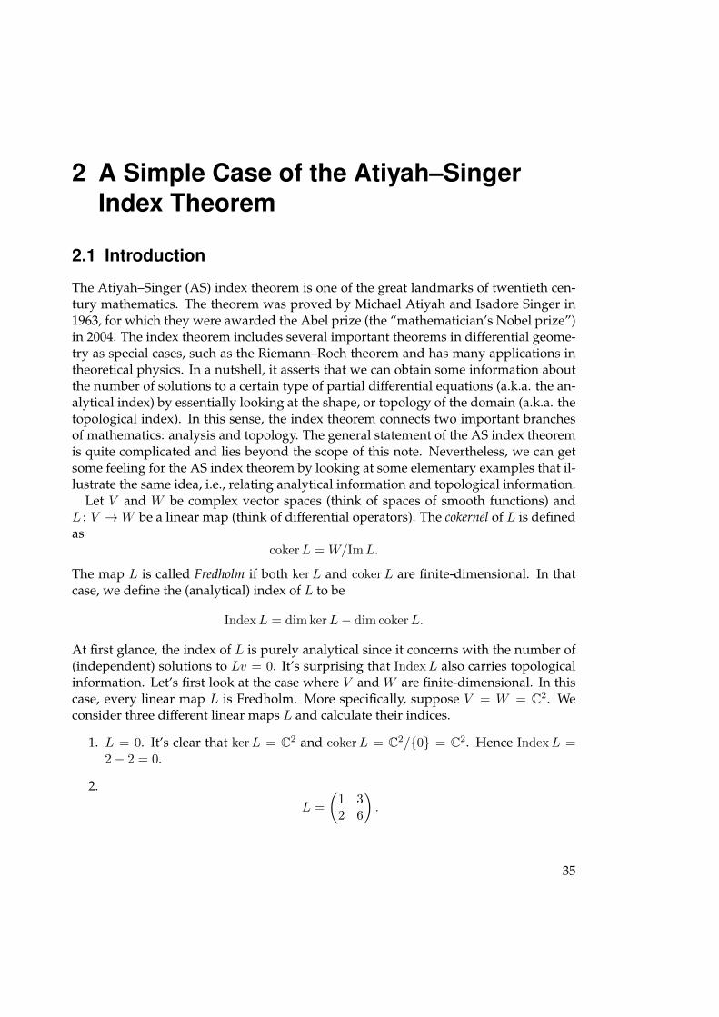
The Atiyah–Singer (AS) index theorem is one of the great landmarks of twentieth cen-tury mathematics. The theorem was proved by Michael Atiyah and Isadore Singer in1963, for which they were awarded the Abel prize (the “mathematician’s Nobel prize”)in 2004. The index theorem includes several important theorems in differential geome-try as special cases, such as the Riemann–Roch theorem and has many applications intheoretical physics. In a nutshell, it asserts that we can obtain some information aboutthe number of solutions to a certain type of partial differential equations (a.k.a. the an-alytical index) by essentially looking at the shape, or topology of the domain (a.k.a. thetopological index). In this sense, the index theorem connects two important branchesof mathematics: analysis and topology. The general statement of the AS index theoremis quite complicated and lies beyond the scope of this note. Nevertheless, we can getsome feeling for the AS index theorem by looking at some elementary examples that il-lustrate the same idea, i.e., relating analytical information and topological information.
Let V and W be complex vector spaces (think of spaces of smooth functions) andL : V →W be a linear map (think of differential operators). The cokernel of L is definedas
cokerL = W/ImL.
The map L is called Fredholm if both kerL and cokerL are finite-dimensional. In thatcase, we define the (analytical) index of L to be
IndexL = dim kerL− dim cokerL.
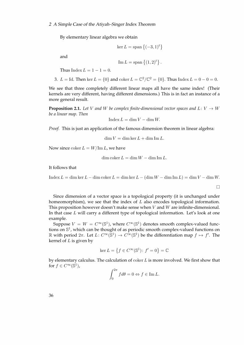
At first glance, the index of L is purely analytical since it concerns with the number of(independent) solutions to Lv = 0. It’s surprising that IndexL also carries topologicalinformation. Let’s first look at the case where V and W are finite-dimensional. In thiscase, every linear map L is Fredholm. More specifically, suppose V = W = C2. Weconsider three different linear maps L and calculate their indices.
1. L = 0. It’s clear that kerL = C2 and cokerL = C2/{0} = C2. Hence IndexL =2− 2 = 0.
2.
L =
(1 32 6
).
35
2 A Simple Case of the Atiyah–Singer Index Theorem
By elementary linear algebra we obtain
kerL = span{
(−3, 1)t}
andImL = span
{(1, 2)t
}.
Thus IndexL = 1− 1 = 0.
3. L = Id. Then kerL = {0} and cokerL = C2/C2 = {0}. Thus IndexL = 0− 0 = 0.
We see that three completely different linear maps all have the same index! (Theirkernels are very different, having different dimensions.) This is in fact an instance of amore general result.
Proposition 2.1. Let V and W be complex finite-dimensional vector spaces and L : V → Wbe a linear map. Then
IndexL = dimV − dimW.
Proof. This is just an application of the famous dimension theorem in linear algebra:
dimV = dim kerL+ dim ImL.
Now since cokerL = W/ImL, we have
dim cokerL = dimW − dim ImL.
It follows that
IndexL = dim kerL− dim cokerL = dim kerL− (dimW − dim ImL) = dimV − dimW.
Since dimension of a vector space is a topological property (it is unchanged underhomeomorphism), we see that the index of L also encodes topological information.This proposition however doesn’t make sense when V and W are infinite-dimensional.In that case L will carry a different type of topological information. Let’s look at oneexample.
Suppose V = W = C∞(S1), where C∞(S1) denotes smooth complex-valued func-tions on S1, which can be thought of as periodic smooth complex-valued functions onR with period 2π. Let L : C∞(S1) → C∞(S1) be the differentiation map f 7→ f ′. Thekernel of L is given by
kerL ={f ∈ C∞(S1) : f ′ = 0
}= C
by elementary calculus. The calculation of cokerL is more involved. We first show thatfor f ∈ C∞(S1), ∫ 2π
0fdθ = 0⇔ f ∈ ImL.
36
2.1 Introduction
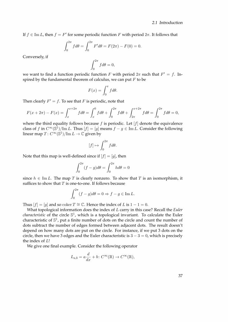
If f ∈ ImL, then f = F ′ for some periodic function F with period 2π. It follows that∫ 2π
0fdθ =
∫ 2π
0F ′dθ = F (2π)− F (0) = 0.
Conversely, if ∫ 2π
0fdθ = 0,
we want to find a function periodic function F with period 2π such that F ′ = f . In-spired by the fundamental theorem of calculus, we can put F to be
F (x) =
∫ x
0fdθ.
Then clearly F ′ = f . To see that F is periodic, note that
F (x+ 2π)− F (x) =
∫ x+2π
xfdθ =
∫ 0
xfdθ +
∫ 2π
0fdθ +
∫ x+2π
2πfdθ =
∫ 2π
0fdθ = 0,
where the third equality follows because f is periodic. Let [f ] denote the equivalenceclass of f in C∞(S1)/ImL. Thus [f ] = [g] means f − g ∈ ImL. Consider the followinglinear map T : C∞(S1)/ImL→ C given by
[f ] 7→∫ 2π
0fdθ.
Note that this map is well-defined since if [f ] = [g], then∫ 2π
0(f − g)dθ =
∫ 2π
0hdθ = 0
since h ∈ ImL. The map T is clearly nonzero. To show that T is an isomorphism, itsuffices to show that T is one-to-one. If follows because∫ 2π
0(f − g)dθ = 0⇒ f − g ∈ ImL.
Thus [f ] = [g] and so cokerT ∼= C. Hence the index of L is 1− 1 = 0.What topological information does the index of L carry in this case? Recall the Euler
characteristic of the circle S1, which is a topological invariant. To calculate the Eulercharacteristic of S1, put a finite number of dots on the circle and count the number ofdots subtract the number of edges formed between adjacent dots. The result doesn’tdepend on how many dots are put on the circle. For instance, if we put 3 dots on thecircle, then we have 3 edges and the Euler characteristic is 3− 3 = 0, which is preciselythe index of L!
We give one final example. Consider the following operator
La,b = ad
dx+ b : C∞(R)→ C∞(R),
37
2 A Simple Case of the Atiyah–Singer Index Theorem
where a and b are arbitrary complex numbers and a 6= 0. The kernel of La,b consists ofthe solutions to the differential equation
ad
dxf + bf = 0.
By separation of variables we obtain
f(x) = Ce−bax, C ∈ C.
Thus dim kerLa,b = 1. To find the cokernel of La,b, we observe that for any f ∈ C∞(R),if we put
F (x) = e−bax
(1
a
∫ x
0ebatf(t)dt
),
thenad
dxF + bF = f.
Thus ImLa,b = C∞(R). It follows that dim cokerLa,b = 0 and hence IndexLa,b = 1 −0 = 1. This example illustrates the fact that the index is stable under deformations.Moreover, the number 1 is also the Euler characteristic of the real line R. (To computethe Euler characteristic of R, we proceed analogously as in the case of S1. However, weneed to discard the two unbounded edges.)
The AS index theorem also finds its applications in Quantum Chromodynamics (QCD),which is a physics theory that studies the behaviors of various subnuclear particles in-teracting via the strong nuclear force, one of the four fundamental forces of nature. TheAS index theorem plays an important role in explaining why certain particles have alarger mass than expected. In the remaining sections, we aim to describe a simple caseof the AS index theorem within the context of gauge theory in theoretical physics. Wefirst need the concept of gauge fields (a.k.a. connections in the mathematics literature).
2.2 Gauge Fields
Consider the complex vector space consisting of all smooth functions R2 → C2. Recallthat a function R2 → C is called smooth if its real and imaginary parts are smooth in theusual sense, i.e., partial derivatives of all orders exist and are continuous. A functionR2 → C2 is smooth if each component function is smooth. Let V denote the vectorsubspace consisting of all smooth functions R2 → C2 satisfying the following twistedperiodicity conditions: {
f(x1 + 1, x2) = f(x1, x2),
f(x1, x2 + 1) = g(x1)f(x1, x2),(2.1)
for x = (x1, x2) ∈ R2 and g(x1) ∈ U(1). Here U(1) is the multiplicative group ofcomplex numbers whose moduli are 1:
U(1) = {z ∈ C : |z| = 1} .
38
2.2 Gauge Fields
Topologically, U(1) is the same as S1, the unit circle in R2. Since g is continuous, thereexists a continuous function θ : R→ R such that
g(x1) = eiθ(x1).
From condition (2.1) we deduce that
f(x1 + 1, x2 + 1) = f(x1, x2 + 1) = eiθ(x1)f(x1, x2)
= eiθ(x1+1)f(x1 + 1, x2) = eiθ(x1+1)f(x1, x2).
Henceθ(x1 + 1) = θ(x1) + 2πQ
for all x1 ∈ R and Q is some integer. (To be more precise, Q should depend on x1.However, since θ is continuous and Q is an integer, it is constant.) With that conditionthe map R→ C given by x1 7→ eiθ(x1) is just a continuous map S1 → S1 and the integerQ is just the winding number (the number of times the map wraps around S1), whichcharacterizes homotopy classes of maps S1 → S1. For an example of V , we can chooseθ(x1) = i2πQx1 for some integer Q. An element of V is
f(x1, x2) =
(ei2πx1(1+Qx2)
ei2πx1(2+Qx2)
).
It’s clear that f satisfies the twisted periodicity condition. (To find such a function, writefj(x1, x2) = ei(p1x1+p2x2) and use the twisted condition to specify p1 and p2.) Finally, wecan turn V into an inner product space by
〈f, g〉 =
∫[0,1]2
g(x)∗f(x)dx for all f, g ∈ V ,
where g(x)∗ denotes the conjugate transpose of g(x) (recall that g(x) is a two-componentcolumn vector) .
We want to define a differential operator on V . However, as we can see, the partialderivatives don’t preserve the condition (2.1):
∂1f(x1, x2 + 1) = ∂1(eiθ(x1)f(x1, x2)) = eiθ(x1)(iθ′(x1)f(x1, x2) + ∂1f(x1, x2)),
which is different from eiθ(x1)∂1(x1, x2). To remedy the situation, we introduce the con-cept of gauge fields. A gauge fieldA can be thought of as a collection of smooth functionsAµ : R2 → R for µ = 1, 2. We replace the partial derivatives by
∇µ : = ∂µ + iAµ for µ = 1, 2.
We want the∇µ to map V to itself, i.e.,
∇µf(x1 + 1, x2) = ∇µf(x1, x2), (2.2)
∇µf(x1, x2 + 1) = eiθ(x1)∇µf(x1, x2) (2.3)
39
2 A Simple Case of the Atiyah–Singer Index Theorem
for all f ∈ V and µ = 1, 2. These requirements will impose certain conditions on thegauge field, as we are about to find out. Let’s first consider requirement (2.2), writingeverything out we obtain
∂µf(x1 + 1, x2) + iAµ(x1 + 1, x2)f(x1 + 1, x2) = ∂µf(x1, x2) + iAµ(x1, x2)f(x1, x2).
Plugging in f(x1 + 1, x2) = f(x1, x2) yields
Aµ(x1 + 1, x2) = Aµ(x1, x2) for µ = 1, 2.
Now for requirement (2.3), writing everything out we obtain
∂µf(x1, x2 + 1) + iAµ(x1, x2 + 1)f(x1, x2 + 1)
= eiθ(x1)(∂µf(x1, x2) + iAµ(x1, x2)f(x1, x2)).
For this case we need to consider µ = 1 and µ = 2. For µ = 1, plugging in f(x1, x2+1) =eiθ(x1)f(x1, x2) yields
∂1(eiθ(x1)f(x1, x2)) + iA1(x1, x2 + 1)eiθ(x1)f(x1, x2)
= eiθ(x1)(∂1f(x1, x2) + iA1(x1, x2)f(x1, x2)).
The left hand side of the above equation becomes
eiθ(x1)(iθ′(x1)f(x1, x2) + ∂1f(x1, x2)) + iA1(x1, x2 + 1)eiθ(x1)f(x1, x2).
Equating with the right hand side we get
A1(x1, x2 + 1) = A1(x1, x2)− θ′(x1).
For the case µ = 2 we have
∂2(eiθ(x1)f(x1, x2)) + iA2(x1, x2 + 1)eiθ(x1)f(x1, x2)
= eiθ(x1)(∂2f(x1, x2) + iA2(x1, x2)f(x1, x2)).
Expanding everything we obtain
A2(x1, x2 + 1) = A2(x1, x2).
To summarize, the gauge field A needs to satisfyA1(x1 + 1, x2) = A1(x1, x2),
A1(x1, x2 + 1) = A1(x1, x2)− θ′(x1),
A2(x1 + 1, x2) = A2(x1, x2),
A2(x1, x2 + 1) = A2(x1, x2).
(2.4)
40
2.3 Gauge Transformations
For an example, if we take θ(x1) = 2πQx1 for some integer Q. It can be verified that thefollowing smooth functions {
A1(x1, x2) = −2πQx2,
A2(x1, x2) = 0
satisfies condition (2.4) of a smooth gauge field. The choice of a gauge field is howeverhighly non-unique. For instance, we can choose{
A1(x1, x2) = −2πQx2 + sin(2π(x1 + x2)),
A2(x1, x2) = sin(2π(x1 + x2)).
Then we have
A1(x1+1, x2) = −2πQx2+sin(2π(x1+1+x2)) = −2πQx2+sin(2π(x1+x2)) = A1(x1, x2),
and
A1(x1, x2 + 1) = −2πQ(x2 + 1) + sin(2π(x1 + x2 + 1))
= −2πQx2 + sin(2π(x1 + x2))− 2πQ
= A1(x1, x2)− θ′(x1).
Clearly A2(x1, x2) is periodic in both directions. In general, we can choose Aµ to be
Aµ(x1, x2) = Aµ(x1, x2) + ϕ(x1, x2),
where ϕ(x1, x2) is periodic in x1 and x2.
2.3 Gauge Transformations
One important type of operations associated with gauge fields is known as gauge trans-formations. A gauge transformation is a smooth map R2 → U(1). We can write this mapas eiφ(x) for some smooth function φ. Our vector space will be transformed into
V ={eiφf : f ∈ V
}.
(Note however that elements of V no longer satisfy the twisted periodicity condition.)The gauge field A will also be transformed into A according to:
∇µ(eiφf) = eiφ∇µf, f ∈ V,
where ∇µ = ∂µ + iAµ. Expanding the left hand side we obtain
∇µ(eiφf) = ∂µ(eiφf) + ieiφAµf
= i(∂µφ)(eiφf) + eiφ∂µf + ieiφAµf
= eiφ[∂µ + i(Aµ + ∂µφ)]f.
Thus Aµ = Aµ − ∂µφ.
41
2 A Simple Case of the Atiyah–Singer Index Theorem
2.4 Topological Charge
Although we have many choices for a gauge field, they all share the following impor-tant property.
Proposition 2.2. The following quantity
1
2π
∫[0,1]2
F12(x1, x2)dx1dx2,
whereF12 =
∂A2
∂x1− ∂A1
∂x2
is an integer and doesn’t depend on the choice of gauge fields.
Proof. We perform a direct computation:∫[0,1]2
(∂A2
∂x1− ∂A1
∂x2
)dx1dx2 =
∫[0,1]2
∂A2
∂x1dx1dx2 −
∫[0,1]2
∂A1
∂x2dx2dx1
=
∫ 1
0(A2(1, x2)−A2(0, x2)) dx2
−∫ 1
0(A1(x1, 1)−A1(x1, 0)) dx1
=
∫ 1
0θ′(x1)dx1 = θ(1)− θ(0)
= 2πQ,
where we’ve used the twisted periodicity conditions (2.4) in the third equality. Theinteger Q obtained is precisely the winding number of x1 7→ eiθ(x1) and hence doesn’tdepend on the gauge field.
We call the integer Q the topological charge of the gauge field A. It’s worthwhile to seehow Q changes under a gauge transformation. Note that
∂1A2 − ∂2A1 = (∂1A2 − ∂1∂2φ)− (∂2A1 − ∂2∂1φ)
= ∂1A2 − ∂2A1
= F12,
where we’ve used (∂1∂2 − ∂2∂1)φ = 0 since φ is smooth. Thus Q is unchanged under agauge transformation. We say that Q is gauge invariant.
2.5 Dirac Operators
In this section we describe a particular class of differential operators which are going tobe our main focus, namely the Dirac operators. In order to define a Dirac operator, we
42
2.5 Dirac Operators
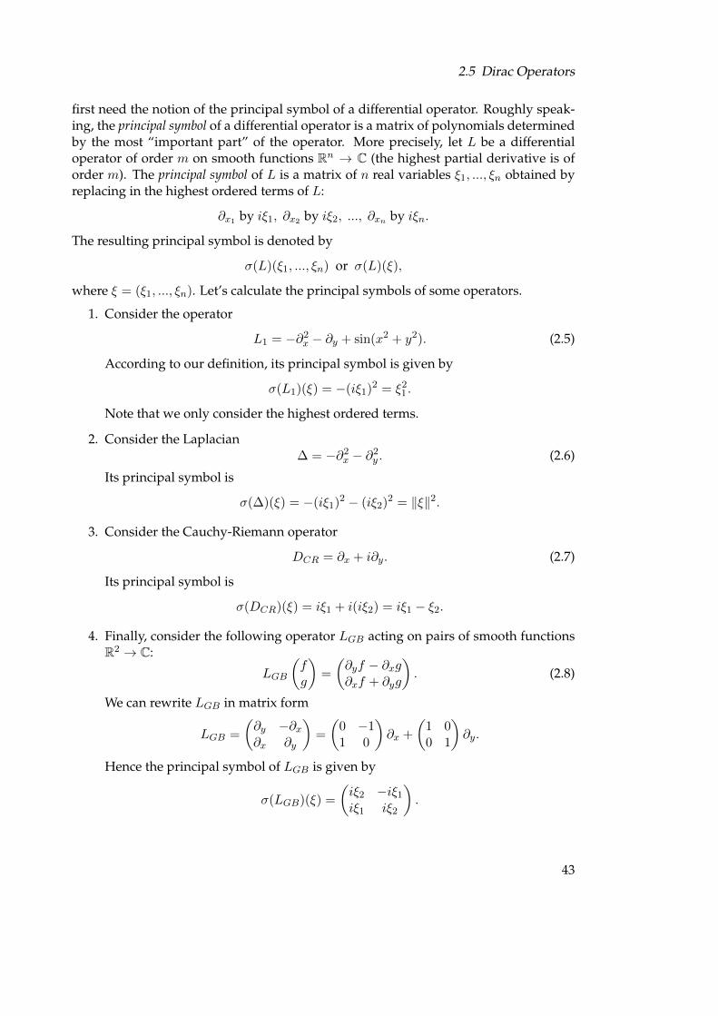
first need the notion of the principal symbol of a differential operator. Roughly speak-ing, the principal symbol of a differential operator is a matrix of polynomials determinedby the most “important part” of the operator. More precisely, let L be a differentialoperator of order m on smooth functions Rn → C (the highest partial derivative is oforder m). The principal symbol of L is a matrix of n real variables ξ1, ..., ξn obtained byreplacing in the highest ordered terms of L:
∂x1 by iξ1, ∂x2 by iξ2, ..., ∂xn by iξn.
The resulting principal symbol is denoted by
σ(L)(ξ1, ..., ξn) or σ(L)(ξ),
where ξ = (ξ1, ..., ξn). Let’s calculate the principal symbols of some operators.
1. Consider the operator
L1 = −∂2x − ∂y + sin(x2 + y2). (2.5)
According to our definition, its principal symbol is given by
σ(L1)(ξ) = −(iξ1)2 = ξ21 .
Note that we only consider the highest ordered terms.
2. Consider the Laplacian∆ = −∂2
x − ∂2y . (2.6)
Its principal symbol is
σ(∆)(ξ) = −(iξ1)2 − (iξ2)2 = ‖ξ‖2.
3. Consider the Cauchy-Riemann operator
DCR = ∂x + i∂y. (2.7)
Its principal symbol is
σ(DCR)(ξ) = iξ1 + i(iξ2) = iξ1 − ξ2.
4. Finally, consider the following operator LGB acting on pairs of smooth functionsR2 → C:
LGB
(fg
)=
(∂yf − ∂xg∂xf + ∂yg
). (2.8)
We can rewrite LGB in matrix form
LGB =
(∂y −∂x∂x ∂y
)=
(0 −11 0
)∂x +
(1 00 1
)∂y.
Hence the principal symbol of LGB is given by
σ(LGB)(ξ) =
(iξ2 −iξ1
iξ1 iξ2
).
43
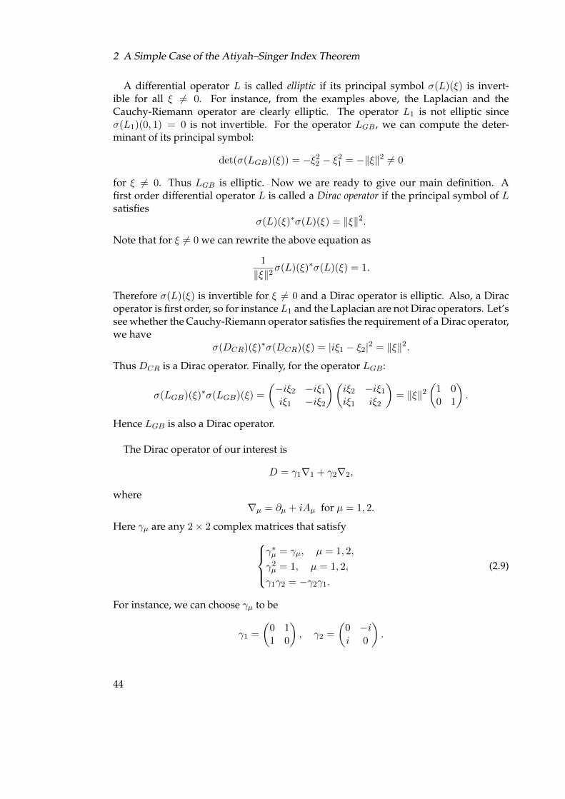
2 A Simple Case of the Atiyah–Singer Index Theorem
A differential operator L is called elliptic if its principal symbol σ(L)(ξ) is invert-ible for all ξ 6= 0. For instance, from the examples above, the Laplacian and theCauchy-Riemann operator are clearly elliptic. The operator L1 is not elliptic sinceσ(L1)(0, 1) = 0 is not invertible. For the operator LGB , we can compute the deter-minant of its principal symbol:
det(σ(LGB)(ξ)) = −ξ22 − ξ2
1 = −‖ξ‖2 6= 0
for ξ 6= 0. Thus LGB is elliptic. Now we are ready to give our main definition. Afirst order differential operator L is called a Dirac operator if the principal symbol of Lsatisfies
σ(L)(ξ)∗σ(L)(ξ) = ‖ξ‖2.
Note that for ξ 6= 0 we can rewrite the above equation as
1
‖ξ‖2σ(L)(ξ)∗σ(L)(ξ) = 1.
Therefore σ(L)(ξ) is invertible for ξ 6= 0 and a Dirac operator is elliptic. Also, a Diracoperator is first order, so for instance L1 and the Laplacian are not Dirac operators. Let’ssee whether the Cauchy-Riemann operator satisfies the requirement of a Dirac operator,we have
σ(DCR)(ξ)∗σ(DCR)(ξ) = |iξ1 − ξ2|2 = ‖ξ‖2.
Thus DCR is a Dirac operator. Finally, for the operator LGB :
σ(LGB)(ξ)∗σ(LGB)(ξ) =
(−iξ2 −iξ1
iξ1 −iξ2
)(iξ2 −iξ1
iξ1 iξ2
)= ‖ξ‖2
(1 00 1
).
Hence LGB is also a Dirac operator.
The Dirac operator of our interest is
D = γ1∇1 + γ2∇2,
where∇µ = ∂µ + iAµ for µ = 1, 2.
Here γµ are any 2× 2 complex matrices that satisfyγ∗µ = γµ, µ = 1, 2,
γ2µ = 1, µ = 1, 2,
γ1γ2 = −γ2γ1.
(2.9)
For instance, we can choose γµ to be
γ1 =
(0 11 0
), γ2 =
(0 −ii 0
).
44
2.6 Chirality
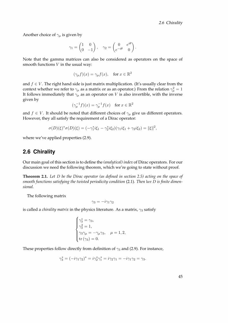
Another choice of γµ is given by
γ1 =
(1 00 −1
), γ2 =
(0 eiθ
e−iθ 0
).
Note that the gamma matrices can also be considered as operators on the space ofsmooth functions V in the usual way:
(γµf)(x) = γµf(x), for x ∈ R2
and f ∈ V . The right hand side is just matrix multiplication. (It’s usually clear from thecontext whether we refer to γµ as a matrix or as an operator.) From the relation γ2
µ = 1It follows immediately that γµ as an operator on V is also invertible, with the inversegiven by
(γ−1µ f)(x) = γ−1
µ f(x) for x ∈ R2
and f ∈ V . It should be noted that different choices of γµ give us different operators.However, they all satisfy the requirement of a Dirac operator:
σ(D)(ξ)∗σ(D)(ξ) = (−γ∗1iξ1 − γ∗2iξ2)(γ1iξ1 + γ2iξ2) = ‖ξ‖2,
where we’ve applied properties (2.9).
2.6 Chirality
Our main goal of this section is to define the (analytical) index of Dirac operators. For ourdiscussion we need the following theorem, which we’re going to state without proof.
Theorem 2.1. Let D be the Dirac operator (as defined in section 2.5) acting on the space ofsmooth functions satisfying the twisted periodicity condition (2.1). Then kerD is finite dimen-sional.
The following matrixγ3 = −iγ1γ2
is called a chirality matrix in the physics literature. As a matrix, γ3 satisfyγ∗3 = γ3,
γ23 = 1,
γ3γµ = −γµγ3, µ = 1, 2,
tr (γ3) = 0.
These properties follow directly from definition of γ3 and (2.9). For instance,
γ∗3 = (−iγ1γ2)∗ = iγ∗2γ∗1 = iγ2γ1 = −iγ1γ2 = γ3.
45
2 A Simple Case of the Atiyah–Singer Index Theorem
For the second property, we have
γ23 = (−iγ1γ2)2 = −γ1γ2γ1γ2 = γ2
1γ22 = 1.
For the third property, for µ = 1,
γ3γ1 = −iγ1γ2γ1 = iγ1γ1γ2 = −γ1γ3,
and for µ = 2,γ3γ2 = −iγ1γ2γ2 = iγ2γ1γ2 = −iγ2γ3.
Finally,tr (γ3) = tr (−iγ1γ2) = tr (iγ2γ1) = tr (iγ1γ2) = −tr (γ3).
Thus tr (γ3) = 0. One important property of γ3 is the following:
γ3D = −Dγ3.
This can be seen by direct calculation. We have
γ3D = γ3(γ1∇1 + γ2∇2) = γ3γ1∇1 + γ3γ2∇2
= −γ1γ3∇1 − γ2γ3∇2 = −(γ1∇1 + γ2∇2)γ3
= −Dγ3.
(Note that γµ as operators on V commute with ∇ν because ∇ν act on the elements ofV component-wise.) One important consequence of the above property is that kerD(known to be finite dimensional) is invariant under γ3, i.e.,
γ3ψ ∈ kerD, for all ψ ∈ kerD.
To see why it’s true, take any ψ ∈ kerD, then
D(γ3ψ) = −γ3D(ψ) = 0.
Thus γ3ψ ∈ kerD. Now we define the projection operators
P+ =1
2(I + γ3), P− =
1
2(I − γ3).
We should check that P± are indeed projections:
P 2+ =
1
4(I + γ3)2 =
1
4(I + 2γ3 + γ2
3) =1
2(I + γ3) = P+,
andP 2− =
1
4(I − γ3)2 =
1
4(I − 2γ3 + γ2
3) =1
2(I − γ3) = P−,
where we’ve used γ23 = 1. Other properties of P± are
P+ + P− =1
2(I + γ3) +
1
2(I − γ3) = I,
46
2.6 Chirality
andP+P− =
1
4(I + γ3)(I − γ3) = 0 = P−P+.
Put (kerD)± = P±(kerD). Since kerD is invariant under γ3, we know that (kerD)± aresubspaces of kerD. Even more is true:
Proposition 2.3.kerD = (kerD)+ ⊕ (kerD)−.
Proof. Take any ψ ∈ kerD, we have
ψ = I(ψ) = (P+ + P−)ψ = P+ψ + P−ψ.
To show the intersection of (kerD)+ and (kerD)− is trivial, take any ψ in the intersec-tion, then
ψ = P+φ1 = P−φ2,
for some φ1, φ2 ∈ kerD. Now apply the properties of P± we obtain
ψ = P+φ1 = P 2+φ1 = P+P−φ2 = 0.
Note that for an element ψ+ ∈ (kerD)+,
γ3ψ+ = γ3P+φ = γ31
2(I + γ3)φ =
1
2(I + γ3)φ = ψ+,
and for an element ψ− ∈ (kerD)−,
γ3ψ− = γ3P−ϕ = γ31
2(I − γ3)ϕ =
1
2(γ3 − I)ϕ = −ψ−.
For this reason, an element in (kerD)+ is said to have positive chirality and an elementin (kerD)− is said to have negative chirality (corresponding to the eigenvalues 1 and −1of γ3, respectively). Now the (analytical) index of D is defined to be the quantity
Index (D) = dim(kerD)+ − dim(kerD)−.
It follows that Index (D) can also be expressed by
Index (D) = tr (γ3 : kerD → kerD).
Under a gauge transformation eiφ, we have
D(eiφf) =∑µ
γµ∇µ(eiφf) = eiφ∑µ
γµ∇µf = eiφDf,
where the second equality follows from a property of gauge transformations. It followsthat
D(eiφf) = 0⇔ Df = 0.
47
2 A Simple Case of the Atiyah–Singer Index Theorem
Thusker D = eiφ kerD.
Consequently,
(ker D)+ = eiφ(kerD)+, (ker D)− = eiφ(kerD)−.
We conclude that Index D is the same as IndexD and hence IndexD is gauge invariant.
2.7 The Atiyah–Singer Index Theorem
Regarding the index of the Dirac operator D, we have the following surprising fact:
Theorem 2.2.Index (D) = −Q.
Recall that Q is the topological charge (section 2.2) associated with our data. Thusthe index of D does not depend on our choice of the gamma matrices and gauge fields!(The dimensions of (kerD)± may be dependent on these factors but their difference isalways a constant.) This theorem is amazing since it tells us that we can extract someinformation about the number of solutions of the system essentially by looking at theshape, or topology, of the domain, without having to actually find the solutions. Inparticular, if Q 6= 0, then we know that the system has to have some solutions. Thisis a special case of the celebrated Atiyah-Singer Index Theorem. The general proof iscomplicated and uses a different technique. In what follows, we attempt to illustratethe theorem for the case of no gauge field A = 0, the topological charge Q = 0 and thefunctions are periodic, i.e., f(x+ eµ) = f(x) for µ = 1, 2.
We first need to talk about hermitian (self-adjoint) operators in infinite-dimensionalvector spaces. Similar to the finite-dimensional case, an operator T on V , the space ofperiodic functions (infinite-dimensional), is called hermitian if
〈Tf, g〉 = 〈f, Tg〉 for all f, g ∈ V .
Analogously, an operator T is anti-hermitian if
〈Tf, g〉 = −〈f, Tg〉 for all f, g ∈ V .
In other words,T ∗ = T.
(We will not discuss the notion of adjoint in general vector space in this note, whichrequires the Riesz representation theorem. More details can be found in [14].) We firstshow that the gamma matrices considered as operators on V are hermitian. Indeed, byproperties of the gamma matrices:
〈γµf, g〉 =
∫[0,1]2
g(x)∗γµf(x)dx =
∫[0,1]2
g(x)∗γ∗µf(x)dx
=
∫[0,1]2
(γµg(x))∗f(x)dx = 〈f, γµg〉 .
48
2.7 The Atiyah–Singer Index Theorem
Slightly more involved is the following proposition, which is true when we restrictourselves to functions satisfying the twisted periodicity condition.
Proposition 2.4. The operators ∂µ are anti-hermitian.
Proof. Since the functions are periodic in one direction and twisted periodic in the otherdirection, we need to consider µ = 1 and µ = 2 separately. First for µ = 1 we have
〈∂1f, g〉 =
∫[0,1]2
g(x)∗∂1f(x)dx
=
∫[0,1]2
[∂1(g(x)∗f(x))− (∂1g(x))∗f(x)] dx (by Leibniz rule)
=
∫ 1
0g(x)∗f(x)
∣∣∣∣x1=1
x1=0
dx2 −∫
[0,1]2(∂1g(x))∗f(x)dx
= −∫
[0,1]2(∂1g(x))∗f(x)dx
= −〈f, ∂1g〉 ,
where we have used g(1, x2)∗f(1, x2) = g(0, x2)∗f(0, x2). Similarly, for µ = 2,
〈∂2f, g〉 =
∫[0,1]2
g(x)∗∂2f(x)dx
=
∫[0,1]2
[∂2(g(x)∗f(x))− (∂2g(x))∗f(x)] dx (by Leibniz rule)
=
∫ 1
0g(x)∗f(x)
∣∣∣∣x2=1
x2=0
dx1 −∫
[0,1]2(∂2g(x))∗f(x)dx
= −∫
[0,1]2(∂2g(x))∗f(x)dx
= −〈f, ∂2g〉 .
Note that here we have
g(x1, 1)∗f(x1, 1)− g(x1, 0)∗f(x1, 0)
= e−iθ(x1)g(x1, 0)∗eiθ(x1)f(x1, 0)− g(x1, 0)∗f(x1, 0) = 0.
One important consequence of the above result is
Corollary 2.1. The Dirac operator is anti-hermitian, i.e.,
D∗ = −D.
49
2 A Simple Case of the Atiyah–Singer Index Theorem
Proof. The Dirac operator is given by
D = γ1∇1 + γ2∇2.
Now∇∗µ = (∂µ + iAµ)∗ = −∂µ − iAµ = −∇µ.
ThusD∗ = −γ1∇1 − γ2∇2 = −D,
where we’ve used the fact that γµ are hermitian.
Now let’s return to our case with A = 0, Q = 0. We want to show that
Index (D) = 0.
We need to investigate the kernel of D. The main theorem is
Theorem 2.3.Dψ = 0⇔ D∗Dψ = 0⇔ ∇∗µ∇µψ = 0⇔ ∇µψ = 0.
Proof. We first prove the first equivalence. Clearly Dψ = 0 implies D∗Dψ = 0. For theother direction, assume that D∗Dψ = 0, then
‖Dψ‖2 = 〈Dψ,Dψ〉 = 〈ψ,D∗Dψ〉 = 〈ψ, 0〉 = 0.
Thus Dψ = 0.For the second equivalence, note that
D∗D = −D2 = − (γ1∇1 + γ2∇2)2
= −(γ2
1∇21 + γ1γ2∇1∇2 + γ2γ1∇2∇1 + γ2
2∇22
)= −
(∇2
1 + γ1γ2∇1∇2 + (−γ1γ2)∇1∇2 +∇22
)= −
(∇2
1 +∇22
)= ∇∗1∇1 +∇∗2∇2.
We have used the fact ∇1∇2 = ∇2∇1 and this is only true in the case where A = 0.(In the general case, they differ by i(∂1A2 − ∂2A1).) Now clearly ∇∗µ∇µψ = 0 implyD∗Dψ = 0. To prove the other direction, consider
〈D∗Dψ,ψ〉 = 〈(∇∗1∇1 +∇∗2∇2)ψ,ψ〉= 〈∇∗1∇1ψ,ψ〉+ 〈∇∗2∇2ψ,ψ〉= 〈∇1ψ,∇1ψ〉+ 〈∇2ψ,∇2ψ〉= ‖∇1ψ‖2 + ‖∇2ψ‖2.
Thus D∗Dψ = 0 implies∇µψ = 0, which in turn implies that∇∗µ∇µψ = 0.Now we prove the third equivalence. It’s clear that ∇µψ = 0 implies ∇∗µ∇µψ = 0.
For the other direction, we have⟨ψ,∇∗µ∇µψ
⟩= 〈∇µψ,∇µψ〉 = ‖∇µψ‖2.
Thus∇∗µ∇µψ = 0 imply∇µψ = 0.
50
2.7 The Atiyah–Singer Index Theorem
We’re now ready to compute the index of D. Since A = 0,∇µ are just ∂µ. Therefore,
Dψ = 0⇔ ∂µψ = 0
for µ = 1, 2. In other words,kerD = C2.
To get the index of D, we need to apply the projection operators P± to kerD. Becauseγ3 6= ±I (tr (γ3) = 0), P±(kerD) 6= 0. Thus
dim(kerD)+ = dim(kerD)− = 1.
Hence,Index (D) = 0.
51
3 Discretization of the Atiyah–SingerIndex Theorem
3.1 Motivations
In this section we give several reasons for developing a discrete version of the Atiyah–Singer index theorem. One of the main motivations comes from gauge theories of par-ticle physics. Various subatomic particles like protons, neutrons etc. are made up ofquarks bound together by the strong nuclear force, which is described by a gauge the-ory called Quantum Chromodynamics (QCD). The index theorem plays an importantrole in explaining why certain subnuclear particles have a larger mass than expected.The calculation of particle masses in the theory requires a discrete lattice formulationof QCD in order to be implemented on a computer. Therefore we need to have indextheorem in discrete setting to get correct masses from lattice QCD calculations.
From the mathematical point of view, discretization is a technique which appearsfrequently. For instance, to solve PDE numerically, we need to discretize the domainand the differential operators. In topology, we can decompose topological spaces intodiscrete “cells” and then can describe some topological invariants combinatorially (theEuler characteristic is a famous example). If a discrete version of the AS index theoremis established, the usual AS index theorem will be recovered in the continuum limit andthat gives us a new proof of the AS index theorem.
In the remaining sections, we’ll develop the discrete counterparts of gauge fields,topological charge, index etc. required for the formulation of the discrete index theo-rem. There may be several ways to discretize a continuous entity. Nevertheless, theyshould all reproduce their continuous counterparts in the continuum limit.
3.2 Lattice Gauge Fields
A lattice on R2 is the following collection of points
L ={
(n1a, n2a) ∈ R2 : (n1, n2) ∈ Z2, a = 1/N}.
Here N is some positive integer. We call an element of the lattice a lattice site and a thelattice spacing. The line segment that connects x and x+aeµ is called a link. The numberof lattice sites on each unit interval is
1
a+ 1 = N + 1.
52
3.2 Lattice Gauge Fields
Here we consider the vector space V of functions L → C2 satisfying the twisted peri-odicity condition: {
f(x1 + 1, x2) = f(x1, x2),
f(x1, x2 + 1) = eiθ(x1)f(x1, x2)(3.1)
for (x1, x2) ∈ L. Similar to the continuum case, the function θ has to satisfy the consis-tency requirement
f(x1 + 1, x2 + 1) = f(x1, x2 + 1) = eiθ(x1)f(x1, x2)
= eiθ(x1+1)f(x1 + 1, x2) = eiθ(x1+1)f(x1, x2).
We deduce thatθ(x1 + 1) = θ(x1) + 2πQ(x1).
Note that in the discrete case, the integer Q doesn’t have to be a constant since thenotion of continuity no longer applies for the function f . We can turn V into an inner-product space by
〈f, g〉 = a2∑x∈Γ
g(x)∗f(x), for f, g ∈ V .
whereΓ = {(n1a, n2a) ∈ L : 0 ≤ n1, n2 < N} .
To justify our definition of the inner product, recall that in the continuum case we have
〈f, g〉 =
∫[0,1]2
g(x)∗f(x)dx = limN→∞
a2∑
0≤n1,n2<N
g(n1a, n2a)∗f(n1a, n2a)
for continuous functions f and g. The discrete inner product satisfies the followingproperty
〈f, g〉 = a2∑x∈Γ
g(x)∗f(x) = a2∑x∈Γ
g(x± aeµ)∗f(x± aeµ), µ = 1, 2, (3.2)
which can be checked by direct computation. Contrary to the continuum case, thevector space V is no longer infinite dimensional since a function on the lattice sites isdetermined by its values on Γ. An orthonormal basis for V can be given by{
δixa
: x ∈ Γ and i = 1, 2
},
where δix is a function on the lattice sites given by
δix(y) = δxyei =
{0 if y 6= x,ei if y = x
for y ∈ Γ and extend to the whole lattice using the boundary conditions. (Here eidenotes the standard basis element of C2.) Thus the dimension of V is 2N2.
53
3 Discretization of the Atiyah–Singer Index Theorem
In the lattice we replace the partial derivative operators by finite-difference operators:
∂µf(x)→ 1
2a[f(x+ aeµ)− f(x− aeµ)].
However, similar to the continuum, the twisted periodicity condition is not preserved.For instance
1
2a[f(x1 + a, x2 + 1)− f(x1 − a, x2 + 1)]
=1
2a[eiθ(x1+a)f(x1 + a, x2)− eiθ(x1−a)f(x1 − a, x2)],
which is different from
1
2aeiθ(x1)[f(x1 + a, x2)− f(x1 − a, x2)].
We need to introduce a lattice version of the gauge field A. By a lattice gauge field Uwe mean a collection of U(1)-valued functions on the links of the lattice. The twistedperiodicity condition will impose certain conditions on U , as we’re going to see below.We’ll use the notation
Figure 3.1: The link variables Uµ(x) and Uµ(x)−1
Uµ(x)↔ U(x, x+ aeµ)
to denote the element of U(1) associated with the link that goes from x+ aeµ to x. Theelement of U(1) associated with a link that goes from x to x + aeµ is naturally definedto be Uµ(x)−1, hence the notation
Uµ(x)−1 ↔ U(x+ aeµ, x).
We also call these Uµ link variables (Figure 3.1). Now the finite-difference operators arereplaced by
∇µf(x) : =1
2a(Uµ(x)f(x+ aeµ)− Uµ(x− aeµ)−1f(x− aeµ)). (3.3)
We can write∇µ as
∇µ =1
2
(∇+µ +∇−µ
),
54
3.3 Relation to Smooth Gauge Fields
where
∇+µ f(x) =
1
a(Uµ(x)f(x+ aeµ)− f(x)),
∇−µ f(x) =1
a(f(x)− Uµ(x− aeµ)−1f(x− aeµ)),
We want the∇µ to map V to itself, i.e.,
∇µf(x1 + 1, x2) = ∇µf(x1, x2),
∇µf(x1, x2 + 1) = eiθ(x1)∇µf(x1, x2)
for all f ∈ V and µ = 1, 2. Proceed analogously as in the continuum case, we obtain thefollowing requirement for the lattice gauge field:
U1(x1 + 1, x2) = U1(x1, x2),
U1(x1, x2 + 1) = eiθ(x1)U1(x1, x2)e−iθ(x1+a),
U2(x1 + 1, x2) = U2(x1, x2),
U2(x1, x2 + 1) = U2(x1, x2).
(3.4)
If we define θ(x1) = 2πQx1 (note that now x1 is a lattice point) for some integer Q, thena lattice gauge field can be given by{
U1(x1, x2) = e−i2πQx2/N ,
U2(x1, x2) = 1.
for (x1, x2) ∈ L. Observe that Uµ(x) is essentially the exponential of Aµ(x). Of coursethe choice of U is not unique, we can replace U by{
U1(x1, x2) = e−i2πQx2/NeiR(x),
U2(x1, x2) = eiR(x),
where R(x) is a real-valued function on the lattice which is periodic in both directions.
3.3 Relation to Smooth Gauge Fields
A lattice gauge field can be obtained from a continuum gauge field by taking transcript.Specifically, Uµ is given by
Uµ(x) = eiαµ(x), where αµ(x) =
∫ a
0Aµ(x+ (a− t)eµ)dt.
Thus αµ(x) is just the integral of Aµ over the link that goes from x+ aeµ to x. When wereverse the direction of the link, the integral will pick up a minus sign. That explainsour notation:
U(x, x+ aeµ) = U(x+ aeµ, x)−1.
55
3 Discretization of the Atiyah–Singer Index Theorem
It can be checked that {Uµ} satisfy the conditions for a lattice gauge field. Indeed,
U1(x1, x2 + 1) = exp
(i
∫ a
0A1(x1 + a− t, x2 + 1)dt
)= exp
(i
∫ a
0(A1(x1 + a− t, x2)− θ′(x1 + a− t))dt
)= exp
(i
∫ a
0A1(x+ (a− t)e1)dt
)exp
(−i∫ a
0θ′(x1 + a− t)dt
)= U1(x1, x2)ei(θ(x1)−θ(x1+a)).
The other conditions can be shown similarly. Since Aµ are smooth, we can use theTaylor expansion around the point x:
Aµ(x+ (a− t)eµ) = Aµ(x) +∂Aµ∂xµ
(x)(a− t) +O((a− t)2).
Hence ∫ a
0Aµ(x+ (a− t)eµ)dt = aAµ(x) +
a2
2
∂Aµ∂xµ
(x) +O(a3).
Now exponentiate both sides we obtain an expansion for Uµ(x)
Uµ(x) = exp
(i
∫ a
0Aµ(x+ (a− t)eµ)dt
)= 1 + i
(aAµ(x) +
a2
2
∂Aµ∂xµ
(x) +O(a3)
)− 1
2
(aAµ(x) +
a2
2
∂Aµ∂xµ
(x) +O(a3)
)2
+ · · ·
= 1 + iaAµ(x) + ia2
2
∂Aµ∂xµ
(x)− a2
2A2µ(x) +O(a3).
Thus up to first order,
Uµ(x) = 1 + iaAµ(x) +O(a2).
Similarly,
U−1µ (x) = 1− iaAµ(x) +O(a2).
When a lattice gauge field U is the transcript of some continuum gauge field A, we’llshow that our discrete operators approach its continuum analogues ∂µ+ iAµ as a tendsto 0 (N tends to ∞). Indeed for a smooth function f , using the expansion of Uµ we
56
3.4 Gauge Transformations on the Lattice
obtain
∇µf(x) =1
2a
(Uµ(x)f(x+ aeµ)− U−1
µ (x− aeµ)f(x− aeµ))
=1
2a(1 + iaAµ(x) +O(a2))f(x+ aeµ)
− 1
2a(1− iaAµ(x− aeµ) +O(a2))f(x− aeµ)
=f(x+ aeµ)− f(x− aeµ)
2a+i
2(Aµ(x)f(x+ aeµ) +Aµ(x− aeµ)f(x− aeµ))
+O(a)(f(x+ aeµ)− f(x− aeµ)).
Thus when a→ 0,∇µf(x)→ ∂µf(x) + iAµ(x)f(x).
3.4 Gauge Transformations on the Lattice
We also have the concept of gauge transformations for lattice gauge fields. Similar tothe continuum case, a gauge transformation is a function from the lattice sites to U(1),which we can write as eiφ(x). Our vector space will be transformed into
V ={eiφf : f ∈ V
}.
The lattice gauge field U will be transformed into U according to:
∇µ(eiφf) = eiφ∇µf.
The left hand side is given by
1
2a
[Uµ(x)eiφ(x+aeµ)f(x+ aeµ)− Uµ(x− aeµ)−1eiφ(x−aeµ)f(x− aeµ)
],
and the right hand side is given by
1
2aeiφ(x)
[Uµ(x)f(x+ aeµ)− Uµ(x− aeµ)−1f(x− aeµ)
].
By comparing the left hand side and the right hand side we obtain
Uµ(x) = eiφ(x)Uµ(x)e−iφ(x+aeµ)
for all lattice sites x and that is how a lattice gauge field is transformed under a gaugetransformation.
In the case where U is the lattice transcript of some smooth gauge field A and eiφ isa gauge transformation in the continuum, we’ll show that the lattice transcript of A is
57
3 Discretization of the Atiyah–Singer Index Theorem
precisely the lattice gauge field U obtained from U by the gauge transformation eiφ (therestriction of eiφ to the lattice sites). Indeed, the lattice transcript of A is given by
eiαµ(x) = exp
(i
∫ a
0Aµ(x+ (a− t)eµ)dt
)= exp
(i
∫ a
0[Aµ(x+ (a− t)eµ)− ∂µφ(x+ (a− t)eµ)] dt
)= exp
(i
∫ a
0Aµ(x+ (a− t)eµ)dt
)exp
(−i∫ a
0∂µφ(x+ (a− t)eµ)dt
)= Uµ(x) exp
(−i∫ a
0∂µφ(x+ (a− t)eµ)dt
).
Now the term ∫ a
0∂µφ(x+ (a− t)eµ)dt = −
∫ldφ = φ(x+ aeµ)− φ(x),
where l is the line segment from x+ aeµ to x and the second equality follows from thefundamental theorem of calculus. Thus
eiαµ(x) = U(x)ei[φ(x)−φ(x+aeµ)] = Uµ(x).
3.5 Naive Index
We can define the Dirac operator in the discrete case as
D = γ1∇1 + γ2∇2.
Here ∇µ are our finite-difference operators (3.3) and the gamma matrices are the sameas in the continuum case. As operators on V , the gamma matrices are hermitian because
〈γµf, g〉 = a2∑x∈Γ
g(x)∗γµf(x) = a2∑x∈Γ
g(x)∗γ∗µf(x)
= a2∑x∈Γ
(γµg(x))∗f(x) = 〈f, γµg〉 .
For any unit vector ψ ∈ V we have
‖γµψ‖2 = 〈γµψ, γµψ〉 =⟨ψ, γ∗µγµψ
⟩= 〈ψ,ψ〉 = 1.
Thus ‖γµ‖ = 1. Since the vector space V is finite-dimensional, kerD is finite-dimensional.The (analytical) index of D can be defined verbatim as in Section 2.6 of Chapter 2. Thus
Index (D) = tr (γ3 : kerV → kerV ).
Naively, if the lattice gauge field is the transcript of some continuum gauge field, wehope that the index ofD will agree with the index of its continuum analogue. However,
58
3.5 Naive Index
it turns out that in the discrete case, the index of D defined in this way is always 0, aswe are going to show below. First, we have (Theorem 1.2)
V = kerD ⊕ (kerD)⊥.
Recall that we haveγ3D = −Dγ3.
Thus kerD is invariant under γ3. As an operator on V , γ3 is hermitian. Moreover sinceγ2
3 = 1 we also have‖γ3‖ = 1.
Now for any w ∈ (kerD)⊥ and z ∈ kerD,
〈γ3w, z〉 = 〈w, γ3z〉 = 0,
where the last equality follows because w ∈ (kerD)⊥ and kerD is invariant under γ3.We conclude that (kerD)⊥ is also invariant under γ3. It follows that
tr (γ3 : V → V ) = tr (γ3 : kerD → kerD) + tr (γ3 : (kerD)⊥ → (kerD)⊥).
We should check that D is anti-hermitian as in the continuum case, i.e.,
D∗ = −D.
For this we need the following property of∇±µ :
Proposition 3.1. (∇±µ)∗
= −∇∓µ .
Proof. It suffices to show that(∇+
µ )∗ = −∇−µ .
Taking the adjoint of both sides we obtain
(∇−µ )∗ = −(∇+µ )∗∗ = −∇+
µ .
Now we have⟨f,−∇−µ g
⟩= a2
∑x∈Γ
(−∇−µ g(x))∗f(x)
= a2∑x∈Γ
(Uµ(x− aeµ)−1g(x− aeµ)− g(x))∗f(x)
= a2∑x∈Γ
(Uµ(x− aeµ)g(x− aeµ)∗ − g(x)∗)f(x)
= a2
(∑x∈Γ
Uµ(x− aeµ)g(x− aeµ)∗f(x)−∑x∈Γ
g(x)∗f(x)
).
59
3 Discretization of the Atiyah–Singer Index Theorem
Note that since U(x) ∈ U(1), we have U(x)−1 = U(x). Now it can be verified by directcomputation that∑
x∈Γ
Uµ(x− aeµ)g(x− aeµ)∗f(x) =∑x∈Γ
Uµ(x)g(x)∗f(x+ aeµ), µ = 1, 2.
Hence
⟨f,−∇−µ g
⟩= a2
(∑x∈Γ
Uµ(x)g(x)∗f(x+ aeµ)−∑x∈Γ
g(x)∗f(x)
)= a2
∑x∈Γ
g(x)∗∇+µ f(x)
=⟨∇+µ f, g
⟩.
Therefore (∇+µ )∗ = −∇−µ .
Proposition 3.2.D∗ = −D.
Proof. Recall that
∇µ =1
2(∇+
µ +∇−µ ).
Thus∇∗µ =
1
2(−∇−µ −∇+
µ ) = −∇µ
for µ = 1, 2. It follows that
D∗ =∑µ
γ∗µ∇∗µ = −∑µ
γµ∇µ = −D.
Now take any v ∈ (kerD)⊥ and w ∈ kerD. Since D is anti-hermitian,
〈Dv,w〉 = 〈v,D∗w〉 = −〈v,Dw〉 = 〈v, 0〉 = 0.
Thus Dv ∈ (kerD)⊥. In other words, (kerD)⊥ is invariant under D. More importantly,
Proposition 3.3. The operator D : (kerD)⊥ → (kerD)⊥ is invertible.
Proof. Since (kerD)⊥ is finite-dimensional, D|(kerD)⊥ is invertible if and only if its ker-
nel is trivial. Take any w ∈ ker(D|(kerD)⊥
), then
D|(kerD)⊥ w = Dw = 0.
Thusw ∈ kerD ∩ (kerD)⊥.
Hence w = 0.
60
3.6 Spectral Flow
Proposition 3.4.tr (γ3 : (kerD)⊥ → (kerD)⊥) = 0.
Proof. To avoid cumbersome notations, in what follows we abbreviate D|(kerD)⊥ to D.We have:
tr (γ3 : (kerD)⊥ → (kerD)⊥) = tr (γ3DD−1) = tr (D−1γ3D)
= −tr (D−1Dγ3 : (kerD)⊥ → (kerD)⊥)
= −tr (γ3 : (kerD)⊥ → (kerD)⊥),
where we’ve used γ3D = −Dγ3 in the second equality. Thus
tr (γ3 : (kerD)⊥ → (kerD)⊥) = 0.
We conclude that
tr (γ3 : V → V ) = tr (γ3 : kerD → kerD).
To finish up, we need to show that
tr (γ3 : V → V ) = 0.
This is a simple exercise in linear algebra. Recall that V has the following orthonormalbasis {
1
aδ1x,
1
aδ2x : x ∈ Γ
},
where δix is a function on the lattice sites given by
δix(y) = δxyei =
{0 if y 6= x,ei if y = x
for y ∈ Γ and extend to the whole lattice using the boundary conditions. Then it’s nothard to verify that with respect to this basis, γ3 is a 2N2× 2N2 (here N is the number oflattice sites) block-diagonal matrix where each block is the matrix γ3. It follows that
tr (γ3 : V → V ) = N2tr (γ3 : C2 → C2) = 0.
3.6 Spectral Flow
In Section 3.5 we see that no matter what the index of the continuum Dirac operatoris, the index of its discrete analogue is always zero. Thus the discrete Dirac operatordoesn’t give any meaningful information about the continuum and that prompts a needfor a new definition of the index. This section aims to motivate our new definition of
61
3 Discretization of the Atiyah–Singer Index Theorem
the index in the lattice setting. The treatment is not entirely rigorous and intuitiveunderstanding is emphasized.
For our new definition of the index, we first need to discuss the notion of the spectralflow. Let H(m) be a family of self-adjoint operators depending smoothly on some realparameter m. (For concreteness, we can take a basis for the vector space and henceH(m) is a family of matrices whose entries are smooth functions of m.) Assume wehave k eigenvalues λ1(m), ..., λk(m) which depend smoothly on m. (The characteristicpolynomial of H(m) is a polynomial whose coefficients are functions of m and we cansolve that polynomial to get the eigenvalues depending on m. These are smooth real-valued functions because the operators are self-adjoint.) Intuitively, the spectral flow ofH(m) in some interval (a, b) is the difference between the number of eigenvalues thatcross the x-axis with positive slope and the number of eigenvalues that cross the x-axis with negative slope, counting multiplicity. (There’s some ambiguity regarding theword multiplicity that we use here. For self-adjoint operators the algebraic multiplicityis the same as the geometric multiplicity and it can be shown that the multiplicity ofλ(m) is constant except for a finite number of points [13].)
The family of operators of our interest is
H(m) = γ3(D −m), m ∈ R,
where D is our naive Dirac operator as defined in Section 3.5. Recall that D is anti-hermitian, i.e.,
D∗ = −D.
Similar to hermitian operators, D can be represented as a diagonal matrix with respectto some orthonormal basis of V . To see why, consider the operator iD, then
(iD)∗ = −iD∗ = iD.
Thus iD is hermitian and so there exists an orthonormal basis for V consisting of eigen-vectors of iD. It follows that D can be expressed as a diagonal matrix with respect tothe same basis. If µ is an eigenvalue of D, then for some nonzero vector v ∈ V ,
µ = 〈Dv, v〉 = 〈v,D∗v〉 = −〈v,Dv〉 = −µ.
Thus an eigenvalue of D is purely imaginary, i.e., it is of the form iλ for some realnumber λ. Moreover,
Proposition 3.5. The eigenvalues of D are symmetric about the real axis.
Proof. We have the relationγ3D = −Dγ3.
Now suppose λ is an eigenvalue of D, i.e., there exists some nonzero vector v ∈ V suchthat
Dv = λv.
62
3.6 Spectral Flow
HenceD(γ3v) = −γ3(Dv) = −γ3(λv) = −λ(γ3v).
It follows that γ3v is an eigenvector of D corresponding to −λ. Since γ3 is invertible,the eigenspaces for λ and −λ are isomorphic and thus λ and −λ have the same multi-plicities.
For any m ∈ R, we have
H(m)2 = γ3(D −m)γ3(D −m) = (−D −m)(D −m) = −D2 +m2,
where we’ve used γ3D = −Dγ3 and γ23 = 1 in the second equality. Choose an or-
thonormal basis for V consisting of eigenvectors of D, then for any element ψ in thatbasis,
H(m)2ψ = (−D2 +m2)ψ = (−(iλ)2 +m2)ψ = (λ2 +m2)ψ.
Thus the eigenvalues of H(m)2 are λ2 +m2 for some real numbers λ. Specifically, theseare the real numbers that satisfy
Dv = iλv
for some nonzero vector v. Note that different λ give us different eigenvalues ofH(m)2.Thus the possible eigenvalues of H(m) are ±
√λ2 +m2. We are interested in those
eigenvalues that cross the x-axis and that occur when
λ2 +m2 = 0.
Since m and λ are real, it is equivalent to λ = m = 0. It follows that the only possibleeigenvalues that cross the x-axis are
f(m) = ±m
and the crossings only occur at the origin. We now compute the spectral flow of H(m)in the interval (−∞,∞). From the above argument, for a fixed m 6= 0,
H(m)ψ = ±mψ
implies thatH(m)2ψ = m2ψ
and so λ = 0 and ψ ∈ kerD. Moreover, for ψ+ ∈ (kerD)+,
H(m)ψ+ = γ3(D −m)ψ+ = −mγ3ψ+ = −mψ+
and for ψ− ∈ (kerD)−,
H(m)ψ− = γ3(D −m)ψ− = −mγ3ψ− = mψ−.
Hence the multiplicity of m is dim(kerD)− and the multiplicity of −m is dim(kerD)+.It follows that
Index (D) = dim(kerD)+ − dim(kerD)−
63
3 Discretization of the Atiyah–Singer Index Theorem
is the difference between the number of eigenvalues of H(m) crossing the x-axis withnegative slope and the number of eigenvalues ofH(m) crossing the x-axis with positiveslope, which is precisely minus the spectral flow of H(m) in (−∞,∞).
In our case of course
dim(kerD)+ = dim(kerD)−
and the spectral flow of H(m) is zero because the index of D is always zero. Hence be-sides the elements of (kerD)±, which we call smooth solutions, that give us the solutionsto D = 0 in the continuum (when we take a → 0), there are elements in (kerD)± thatdon’t correspond to any solutions of D = 0 in the continuum and we call those roughsolutions. To get a meaningful definition of the index in the lattice setting, we need away to separate the rough and smooth solutions. We do that by introducing a modifiedversion of our naive Dirac operator, the so called Wilson-Dirac operator:
Dw = D +a
2∆.
Here ∆ is a lattice version of the second derivative:
∆ =∑µ=1,2
∆µ, ∆µ = −∇+µ∇−µ .
The explicit formula for ∆µ is given by
∆µf(x) =1
a2(−Uµ(x)f(x+ aeµ) + 2f(x)− Uµ(x− aeµ)−1f(x− aeµ)).
The operator ∆ has several important properties.
Proposition 3.6.
∆µ = −∇+µ∇−µ = −∇−µ∇+
µ =1
a(∇−µ −∇+
µ ).
Proof. These equalities follow from direct computation. We have:
∇+µ (∇−µ f)(x) =
1
a(Uµ(x)∇−µ f(x+ aeµ)−∇−µ f(x))
=1
a
[Uµ(x)
(1
a
[f(x+ aeµ)− Uµ(x)−1f(x)
])−(
1
a
[f(x)− Uµ(x− aeµ)−1f(x− aeµ)
])]=
1
a2
[Uµ(x)f(x+ aeµ)− 2f(x) + Uµ(x− aeµ)−1f(x− aeµ)
],
64
3.6 Spectral Flow
and
∇−µ (∇+µ f)(x) =
1
a(∇+
µ f(x)− Uµ(x− aeµ)−1∇+µ f(x− aeµ))
=1
a
[(1
a[Uµ(x)f(x+ aeµ)− f(x)]
)− Uµ(x− aeµ)−1
(1
a[Uµ(x− aeµ)f(x)− f(x− aeµ)]
)]=
1
a2
[Uµ(x)f(x+ aeµ)− 2f(x) + Uµ(x− aeµ)−1f(x− aeµ)
].
Finally,
1
a(∇+
µ −∇−µ )f(x) =1
a
(1
a[Uµ(x)f(x+ aeµ)− f(x)]
− 1
a
[f(x)− Uµ(x− aeµ)−1f(x− aeµ)
])=
1
a2
[Uµ(x)f(x+ aeµ)− 2f(x) + Uµ(x− aeµ)−1f(x− aeµ)
].
Proposition 3.7. The operator ∆ is positive, i.e., ‖∆‖ ≥ 0. Here ‖ ‖ denotes the operator norm(Section 1.3). In particular, ∆ is hermitian.
Proof. Proceed by definition of positive operators:
〈∆µf, f〉 =⟨−∇+
µ∇−µ f, f⟩
=⟨∇−µ f, (−∇+
µ )∗f⟩
=⟨∇−µ f,∇−µ f
⟩≥ 0,
where we again use Proposition 3.1. Since sums of positive operators are positive, ∆ ispositive.
Unlike the naive Dirac operator D, Dw is no longer anti-hermitian:
D∗w =(D +
a
2∆)∗
= −D +a
2∆.
And the relation γ3D = −Dγ3 becomes
γ3Dw = γ3
(D +
a
2∆)
= −Dγ3 +a
2∆γ3 = D∗wγ3.
Note that ∆ and γ3 commute since ∆ does not contain any gamma matrices. Thisequality means that kerDw is no longer invariant under γ3 and hence we can’t definethe index of Dw in terms of chirality. The positivity of ∆ has another consequence:suppose m is a real eigenvalue of Dw, i.e.,
Dwψ = mψ
for some nonzero vector ψ ∈ V such that ‖ψ‖ = 1. Then
〈a∆ψ,ψ〉 = 〈(Dw +D∗w)ψ,ψ〉 = 〈Dwψ,ψ〉+ 〈ψ,Dwψ〉 = 2m.
Since ∆ is positive, we conclude that m ≥ 0. Thus Dw has only non-negative realeigenvalues.
65
3 Discretization of the Atiyah–Singer Index Theorem
3.7 Hermitian Wilson-Dirac Operator
Similar to the Dirac operator we consider the following family of operators:
Hw(m) = γ3(Dw −m), m ∈ R.
Using the relation γ3Dw = D∗wγ3, we have
Hw(m)∗ = (D∗w −m)γ∗3 = γ3(Dw −m) = Hw(m).
Thus Hw(m) is hermitian and so all its eigenvalues are real. We are interested in theeigenvalue flow of Hw(m). First, if
Hw(m)ψ = 0
for some nonzero vector ψ ∈ V , then
Dwψ = mψ.
So m is an eigenvalue of Dw. Thus the eigenvalues of Hw(m) cross the x-axis at realeigenvalues ofDw. Since real eigenvalues ofDw are non-negative, eigenvalue crossingsof Hw(m) can only occur when m ≥ 0. Another important property of the eigenvaluesof Hw(m) is given by the next proposition.
Proposition 3.8. Let λ(m) be an eigenvalue of Hw(m), then
|λ′(m)| ≤ 1.
Proof. We haveH(m)ψ(m) = λ(m)ψ(m),
where ψ(m) also depends smoothly on m and ‖ψ(m)‖ = 1 (think of ψ(m) as a vectorwhose entries are smooth functions of m). Thus
〈H(m)ψ(m), ψ(m)〉 = λ(m) 〈ψ(m), ψ(m)〉 = λ(m).
Now we can differentiate λ(m):
λ′(m) = limh→0
1
h(〈H(m+ h)ψ(m+ h), ψ(m+ h)〉 − 〈H(m)ψ(m), ψ(m)〉)
= limh→0
1
h(〈H(m+ h)ψ(m+ h), ψ(m+ h)〉 − 〈H(m+ h)ψ(m+ h), ψ(m)〉
+ 〈H(m+ h)ψ(m+ h), ψ(m)〉 − 〈H(m)ψ(m+ h), ψ(m)〉+ 〈H(m)ψ(m+ h), ψ(m)〉 − 〈H(m)ψ(m), ψ(m)〉)
=⟨H(m)ψ(m), ψ′(m)
⟩+⟨H ′(m)ψ(m), ψ(m)
⟩+⟨H(m)ψ′(m), ψ(m)
⟩.
Now note that⟨H(m)ψ′(m), ψ(m)
⟩=⟨ψ′(m), H(m)ψ(m)
⟩= λ(m)
⟨ψ′(m), ψ(m)
⟩.
66
3.7 Hermitian Wilson-Dirac Operator
Thus λ′(m) becomes
λ′(m) = λ(m)(⟨ψ(m), ψ′(m)
⟩+⟨ψ′(m), ψ(m)
⟩)+⟨H ′(m)ψ(m), ψ(m)
⟩.
Now we have
d
dm‖ψ(m)‖2 =
d
dm〈ψ(m), ψ(m)〉 =
⟨ψ′(m), ψ(m)
⟩+⟨ψ(m), ψ′(m)
⟩.
Since ‖ψ(m)‖2 = 1, its derivative is 0. Thus
λ′(m) =⟨H ′(m)ψ(m), ψ(m)
⟩.
Moreover,
H ′(m) =d
dmγ3(Dw −m) = −γ3.
Consequently,λ′(m) = −〈γ3ψ(m), ψ(m)〉 .
Now by Cauchy–Schwarz inequality,
|λ′(m)| ≤ ‖γ3ψ(m)‖‖ψ(m)‖ = ‖γ3ψ(m)‖ ≤ 1
since‖γ3ψ(m)‖ ≤ ‖γ3‖‖ψ(m)‖ = 1
(recall that ‖γ3‖ = 1).
As was mentioned previously, the introduction of ∆ was meant to separate the smoothand rough solutions to Dψ = 0. The separation is going to be reflected in the spectralflow of Hw(m). To illustrate the idea, we consider the case where there is no gaugefield. In the continuum, that corresponds to A = 0, the functions are periodic in bothdirections and in the discrete setting U = 1. Recall that the equation Dψ = 0 hasonly the constant solutions in the continuum (Theorem 2.3). However, as we know,the discretized equation Dψ = 0 will produce rough solutions. These solutions can becomputed explicitly. First we have the following observation
Proposition 3.9. The following collection of functions on the lattice{eipxei : p = (2πk1, 2πk2), 0 ≤ k1, k2 < N, x ∈ L, i = 1, 2
}form an orthonormal basis for V . (Here px = p1x1 + p2x2.)
Proof. We first notice that
eip(x+eµ) = eipx+ipµ = eipxeipµ = eipx
67
3 Discretization of the Atiyah–Singer Index Theorem
since pµ = 2πkµ for some integer kµ. Hence these functions are periodic. If they are alldistinct, then there are 2N2 functions, which is precisely the dimension of V . To showthat they form an orthonormal basis, it suffices to show that
⟨eipx, eiqx
⟩= δpq =
{1 if p = q,
0 if p 6= q.
By the definition of the inner product,⟨eipx, eipx
⟩= a2
∑x∈Γ
e−ipxeipx = a2N2 = 1.
When p 6= q, put (k1, k2) = q − p 6= (0, 0) we have⟨eipx, eiqx
⟩= a2
∑x∈Γ
e−ipxeiqx = a2∑x∈Γ
ei(q−p)x
= a2∑x∈Γ
ei(2πak1n1+2πak2n2) (here ni = xi/a)
= a2N−1∑n1=0
(ei2πak1
)n1N−1∑n2=0
(ei2πak2
)n2
.
Now suppose k1 6= 0, then
N−1∑n1=0
(ei2πak1
)n1
=
(1−
(ei2πak1
)N1− ei2πak1
)= 0,
where the last equality follows because(ei2πak1
)N= ei2πak1N = 1.
To find solutions to Dψ = 0, recall that Dψ = 0 if and only if D∗D = 0 and
D∗D =∑µ
γµ∇∗µ∑ν
γν∇ν = −∑µ
γµ∇µ∑ν
γν∇ν = −∑µ
∇2µ.
In the case where U = 1 we have
∇µeipx =1
2a
(eip(x+aeµ) − eip(x−aeµ)
)=i
asin(apµ)eipx.
Thus we obtain a complete list of eigenvalues of∇µ. It follows that
D∗Deipx =1
a2
∑µ
sin2(apµ)eipx.
(Note that here we omit the unit vector ei for simplicity.) Hence D∗Deipx = 0 if andonly if sin(apµ) = 0 for all µ. The latter equations imply that pµ ∈ {0, π/a} (recall that0 ≤ kµ < N ). Therefore
p ∈ {(0, 0), (π/a, 0), (0, π/a), (π/a, π/a)}
68
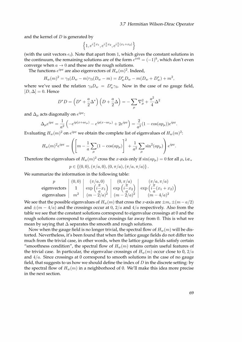
3.7 Hermitian Wilson-Dirac Operator
and the kernel of D is generated by{1, ei
πax1 , ei
πax2 , ei
πa
(x1+x2)}
(with the unit vectors ei). Note that apart from 1, which gives the constant solutions inthe continuum, the remaining solutions are of the form eiπk = (−1)k, which don’t evenconverge when a→ 0 and these are the rough solutions.
The functions eipx are also eigenvectors of Hw(m)2. Indeed,
Hw(m)2 = γ3(Dw −m)γ3(Dw −m) = D∗wDw −m(Dw +D∗w) +m2,
where we’ve used the relation γ3Dw = D∗wγ3. Now in the case of no gauge field,[D,∆] = 0. Hence
D∗D =(D∗ +
a
2∆∗)(
D +a
2∆)
= −∑µ
∇2µ +
a2
4∆2
and ∆µ acts diagonally on eipx:
∆µeipx =
1
a2
(−eip(x+aeµ) − eip(x−aeµ) + 2eipx
)=
2
a2(1− cos(apµ))eipx.
Evaluating Hw(m)2 on eipx we obtain the complete list of eigenvalues of Hw(m)2:
Hw(m)2eipx =
[m− 1
a
∑µ
(1− cos(apµ)
]2
+1
a2
∑µ
sin2(apµ)
eipx.
Therefore the eigenvalues of Hw(m)2 cross the x-axis only if sin(apµ) = 0 for all µ, i.e.,
p ∈ {(0, 0), (π/a, 0), (0, π/a), (π/a, π/a)} .
We summarize the information in the following table:
p (0, 0) (π/a, 0) (0, π/a) (π/a, π/a)
eigenvectors 1 exp(iπ
ax1
)exp
(iπ
ax2
)exp
(iπ
a(x1 + x2)
)eigenvalues m2 (m− 2/a)2 (m− 2/a)2 (m− 4/a)2
We see that the possible eigenvalues of Hw(m) that cross the x-axis are±m,±(m−a/2)and ±(m − 4/a) and the crossings occur at 0, 2/a and 4/a respectively. Also from thetable we see that the constant solutions correspond to eigenvalue crossings at 0 and therough solutions correspond to eigenvalue crossings far away from 0. This is what wemean by saying that ∆ separates the smooth and rough solutions.
Now when the gauge field is no longer trivial, the spectral flow of Hw(m) will be dis-torted. Nevertheless, it’s been found that when the lattice gauge fields do not differ toomuch from the trivial case, in other words, when the lattice gauge fields satisfy certain“smoothness condition”, the spectral flow of Hw(m) retains certain useful features ofthe trivial case. In particular, the eigenvalue crossings of Hw(m) occur close to 0, 2/aand 4/a. Since crossings at 0 correspond to smooth solutions in the case of no gaugefield, that suggests to us how we should define the index ofD in the discrete setting: bythe spectral flow of Hw(m) in a neighborhood of 0. We’ll make this idea more precisein the next section.
69
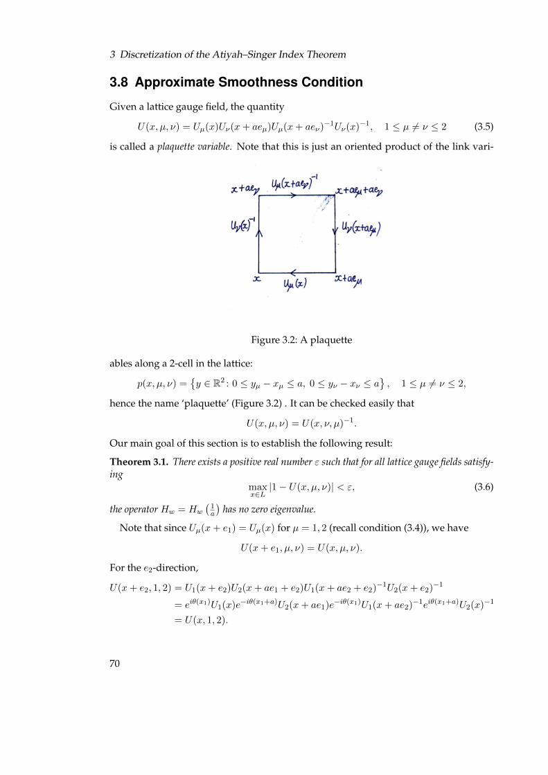
3 Discretization of the Atiyah–Singer Index Theorem
3.8 Approximate Smoothness Condition
Given a lattice gauge field, the quantity
U(x, µ, ν) = Uµ(x)Uν(x+ aeµ)Uµ(x+ aeν)−1Uν(x)−1, 1 ≤ µ 6= ν ≤ 2 (3.5)
is called a plaquette variable. Note that this is just an oriented product of the link vari-
Figure 3.2: A plaquette
ables along a 2-cell in the lattice:
p(x, µ, ν) ={y ∈ R2 : 0 ≤ yµ − xµ ≤ a, 0 ≤ yν − xν ≤ a
}, 1 ≤ µ 6= ν ≤ 2,
hence the name ‘plaquette’ (Figure 3.2) . It can be checked easily that
U(x, µ, ν) = U(x, ν, µ)−1.
Our main goal of this section is to establish the following result:
Theorem 3.1. There exists a positive real number ε such that for all lattice gauge fields satisfy-ing
maxx∈L|1− U(x, µ, ν)| < ε, (3.6)
the operator Hw = Hw
(1a
)has no zero eigenvalue.
Note that since Uµ(x+ e1) = Uµ(x) for µ = 1, 2 (recall condition (3.4)), we have
U(x+ e1, µ, ν) = U(x, µ, ν).
For the e2-direction,
U(x+ e2, 1, 2) = U1(x+ e2)U2(x+ ae1 + e2)U1(x+ ae2 + e2)−1U2(x+ e2)−1
= eiθ(x1)U1(x)e−iθ(x1+a)U2(x+ ae1)e−iθ(x1)U1(x+ ae2)−1eiθ(x1+a)U2(x)−1
= U(x, 1, 2).
70

3.8 Approximate Smoothness Condition
HenceU(x+ ek, µ, ν) = U(x, µ, ν), k = 1, 2.
It follows that we can restrict our attention to these lattice sites x ∈ Γ in (3.6). Condition(3.6) is also called the approximate smoothness condition. Since the plaquette variablesare unchanged under gauge transformations, gauge transformations don’t change thesmoothness condition.
The proof is unfortunately long and we need to make some preparations. We intro-duce the following operators on V{
T+µ ψ(x) = Uµ(x)ψ(x+ aeµ),
T−µ ψ(x) = Uµ(x− aeµ)−1ψ(x− aeµ).
We have
T+µ (T−µ ψ)(x) = Uµ(x)T−µ ψ(x+ aeµ) = Uµ(x)Uµ(x)−1ψ(x) = ψ(x)
and similarly,
T−µ (T+µ ψ)(x) = Uµ(x− aeµ)−1T+
µ ψ(x− aeµ) = Uµ(x− aeµ)−1Uµ(x− aeµ)ψ(x) = ψ(x).
Therefore,T+µ T−µ = T−µ T
+µ = I.
One nice property of these operators is that they all have unit norm. Indeed, chooseany ψ ∈ V such that ‖ψ‖ = 1, then
‖T−µ ψ‖2 =⟨T−µ ψ, T
−µ ψ⟩
= a2∑x∈Γ
[T−µ ψ(x)]∗T−µ ψ(x)
= a2∑x∈Γ
Uµ(x− aeµ)ψ(x− aeµ)∗Uµ(x− aeµ)−1ψ(x− aeµ)
= ‖ψ‖2 = 1,
where we’ve used the fact that Uµ(x− aeµ) = Uµ(x − aeµ)−1 in U(1). It can be shownsimilarly that ‖T+
µ ‖ = 1. We are going to need the commutators of T±µ , so we computethem here:
[T+µ , T
−ν ]ψ(x) = T+
µ (T−ν ψ)(x)− T−ν (T+µ ψ)(x)
= Uµ(x)T−ν ψ(x+ aeµ)− Uν(x− aeν)−1T+µ ψ(x− aeν)
= Uµ(x)Uν(x+ aeµ − aeν)−1ψ(x+ aeµ − aeν)
− Uν(x− aeν)−1Uµ(x− aeν)ψ(x− aeν + aeµ)
= (Uµ(x)Uν(x+ aeµ − aeν)−1 − Uν(x− aeν)−1Uµ(x− aeν))ψ(x− aeν + aeµ)
= Uν(x− aeν)−1(U(x− aeν , ν, µ)− 1)Uµ(x− aeν)ψ(x− aeν + aeµ).
71
3 Discretization of the Atiyah–Singer Index Theorem
Similarly, it can be verified that
[T+µ , T
+ν ]ψ(x) = (U(x, µ, ν)− 1)Uν(x)Uµ(x+ aeν)ψ(x+ aeν + aeµ)
and
[T−µ , T−ν ]ψ(x) = Uν(x−aeν)−1Uµ(x−aeµ−aeν)−1(U(x−aeν−aeµ, µ, ν)−1)ψ(x−aeµ−aeν).
Note that in terms of the left, right difference operators:
∇+µ =
1
a(T+µ − I), ∇−µ =
1
a(I − T−µ ).
Hence∇µ =
1
2(∇+
µ +∇−µ ) =1
2a(T+µ − T−µ ),
and∆µ =
1
a(∇−µ −∇+
µ ) =1
a2(−T+
µ − T−µ + 2I).
Written in terms of T±µ , we obtain several nice relations between∇µ and ∆µ.
Proposition 3.10.
−∇2µ +
a2
4∆2µ −∆µ = 0.
Proof. Put
Sµ =1
2i(T+µ − T−µ ), Cµ =
1
2(T+µ + T−µ ).
ThenS2µ + C2
µ = I,
where we’ve used T+µ T−µ = T−µ T
+µ = I . (Note the similarity with sine and cosine.)
Now,
∇µ =1
2a(T+µ − T−µ ) =
i
aSµ,
and∆µ =
1
a2(−T+
µ − T−µ + 2I) = − 2
a2Cµ +
2
a2.
Plug everything in the left hand side of the equality we get 0.
Proposition 3.11.[∇µ,∆µ] = 0.
Proof. We have
[∇µ,∆µ] =
[1
2a(T+µ − T−µ ),
1
a2(−T+
µ − T−µ + 2I)
].
Now it’s clear that:[T+µ , I] = [T−µ , I] = 0,
72
3.8 Approximate Smoothness Condition
and
[T+µ , T
−µ ] = T+
µ T−µ − T−µ T+
µ = I − I = 0.
We’re now ready to prove our theorem. It suffices to show that H2w has no zero
eigenvalue, i.e.,
‖H2wψ‖ > 0
for all ψ ∈ V such that ‖ψ‖ = 1. First we compute H2w:
H2w = γ3
(Dw −
1
a
)γ3
(Dw −
1
a
)=
(D∗w −
1
a
)(Dw −
1
a
)=
(−D +
a
2∆− 1
a
)(D +
a
2∆− 1
a
)= −D2 +
a
2(−D∆ + ∆D) +
(a
2∆− 1
a
)2
= −D2 − a
2[D,∆] +
(a
2∆− 1
a
)2
,
where in the second equality we’ve used γ3Dw = −D∗wγ3 and γ23 = 1. Now we evaluate
each term of the right hand side. We have:
D2 =∑µ
γµ∇µ∑ν
γν∇ν
=∑µ
∇2µ +
∑µ6=ν
γµγν∇µ∇ν (since γ2µ = 1)
=∑µ
∇2µ +
∑µ>ν
γµγν [∇µ,∇ν ] (since γµγν = −γνγµ),
and
[D,∆] =
[∑µ
γµ∇µ,∆
]=∑µ
γµ[∇µ,∆]
=∑µ
[∇µ,
∑ν
∆ν
]=∑µ 6=ν
γµ[∇µ,∆ν ],
73
3 Discretization of the Atiyah–Singer Index Theorem
where we’ve used [∇µ,∆µ] = 0 in the last equality. Finally,(a
2∆− 1
a
)2
=a2
4∆2 −∆ +
1
a2
=a2
4
(∑µ
∆µ
)2
−∑µ
∆µ +1
a2
=a2
4
∑µ
∆2µ +
a2
4
∑µ6=ν
∆µ∆ν −∑µ
∆µ +1
a2.
Note that generally ∆µ∆ν 6= ∆ν∆µ. Hence the operator H2w becomes
H2w = −
∑µ
∇2µ −
∑µ>ν
γµγν [∇µ,∇ν ]− a
2
∑µ6=ν
γµ[∇µ,∆ν ]
+a2
4
∑µ
∆2µ +
a2
4
∑µ6=ν
∆µ∆ν −∑µ
∆µ +1
a2
=∑µ
(−∇2
µ +a2
4∆2µ −∆µ
)−∑µ>ν
γµγν [∇µ,∇ν ]
− a
2
∑µ6=ν
γµ[∇µ,∆ν ] +a2
4
∑µ6=ν
∆µ∆ν +1
a2
= −∑µ>ν
γµγν [∇µ,∇ν ]− a
2
∑µ 6=ν
γµ[∇µ,∆ν ] +a2
4
∑µ 6=ν
∆µ∆ν +1
a2,
where in the last equality we’ve used
−∇2µ +
a2
4∆2µ −∆µ = 0.
Now we can write ∆µ∆ν as
∆µ∆ν =(∇+µ
)∗∇+µ∆ν
=(∇+µ
)∗[∇+
µ∆ν −∆ν∇+µ + ∆ν∇+
µ ]
=(∇+µ
)∗[∇+
µ ,∆ν ] +(∇+µ
)∗∆ν∇+
µ .
Put Pµν =(∇+µ
)∗∆ν∇+
µ , then Pµν is positive since
〈Pµνψ,ψ〉 =⟨(∇+µ
)∗∆ν∇+
µψ,ψ⟩
=⟨∆ν(∇+
µψ),∇+µψ⟩≥ 0
because ∆ν is positive. Thus we can write H2w as
H2w =
1
a2+ P −
∑µ>ν
γµγν [∇µ,∇ν ]− a
2
∑µ 6=ν
γµ[∇µ,∆ν ] +a2
4
∑µ 6=ν
(∇+µ
)∗[∇+
µ ,∆ν ]
74
3.8 Approximate Smoothness Condition
where P is a positive operator. Now for any vector ψ ∈ V with ‖ψ‖ = 1,
‖H2wψ‖ ≥
∥∥∥∥( 1
a2+ P
)ψ
∥∥∥∥−∑µ>ν
‖γµγν [∇µ,∇ν ]ψ‖ − a
2
∑µ6=ν‖γµ[∇µ,∆ν ]ψ‖
− a2
4
∑µ6=ν
∥∥(∇+µ )∗[∇+
µ ,∆ν ]ψ∥∥ .
Now since P is positive,∥∥∥∥( 1
a2+ P
)ψ
∥∥∥∥2
=
⟨(1
a2+ P
)ψ,
(1
a2+ P
)ψ
⟩=
⟨1
a2ψ,
1
a2ψ
⟩+
⟨1
a2ψ, Pψ
⟩+
⟨Pψ,
1
a2ψ
⟩+ 〈Pψ, Pψ〉
≥∥∥∥∥ 1
a2ψ
∥∥∥∥2
=1
a2.
Also we have the following (recall that ‖ψ‖ = 1 and ‖γµ‖ = 1):
‖γµγν [∇µ,∇ν ]ψ‖ ≤ ‖γµ‖‖γν‖ ‖[∇µ,∇ν ]‖ ‖ψ‖ = ‖[∇µ,∇ν ]‖ ,
and‖γµ[∇µ,∆ν ]ψ‖ ≤ ‖γµ‖ ‖[∇µ,∆ν ]‖ ‖ψ‖ = ‖∇µ,∆ν‖ ,
and ∥∥(∇+µ )∗[∇+
µ ,∆ν ]ψ∥∥ ≤ ∥∥(∇+
µ )∗∥∥ ‖[∇+
µ ,∆ν ]‖‖ψ‖ ≤ 2
a‖[∇+
µ ,∆ν ]‖,
where
‖(∇+µ )∗‖ = ‖∇−µ ‖ =
∥∥∥∥1
a(I − T−µ )
∥∥∥∥ ≤ 1
a(1 + ‖T−µ ‖) =
2
a.
(Recall that ‖T±µ ‖ = 1.) Consequently,
‖H2wψ‖ ≥
1
a2−∑µ>ν
‖[∇µ,∇ν ]‖ − a
2
∑µ 6=ν‖[∇µ,∆ν ]‖ − a
2
∑µ6=ν‖[∇+
µ ,∆ν ]‖.
Now note that
[∇+µ ,∇−µ ] =
[1
a(T+µ − I),
1
a(I − T−ν )
]= − 1
a2[T+µ , T
−ν ],
[∇+µ ,∇+
ν ] =
[1
a(T+µ − I),
1
a(T+ν − I)
]=
1
a2[T+µ , T
+ν ],
[∇−µ ,∇−ν ] =
[1
a(I − T−µ ),
1
a(I − T−ν )
]=
1
a2[T−µ , T
−ν ].
75
3 Discretization of the Atiyah–Singer Index Theorem
Thus we need to investigate the norms of the commutators of T±µ . Put R = [T+µ , T
−ν ].
Then for any vector ψ ∈ V such that ‖ψ‖ = 1, we have
‖Rψ‖2 = 〈Rψ,Rψ〉 = a2∑x∈Γ
Rψ(x)∗Rψ(x)
= a2∑x∈Γ
|U(x− aeν , ν, µ)− 1|2ψ(x)∗ψ(x)
< maxx∈Γ|U(x− aeν , ν, µ)− 1|2 = ε2.
Thus ‖[T+µ , T
−ν ]‖ < ε. Similarly we can show that∥∥[T+
µ , T+ν ]∥∥ < ε,
∥∥[T−µ , T−ν ]∥∥ < ε.
Now we can bound the commutators:
‖[∇µ,∇ν ]‖ =
∥∥∥∥[1
2(∇+
µ +∇−µ ),1
2(∇+
µ +∇−ν )
]∥∥∥∥ ≤ 1
4
(4× 1
a2ε
)=
ε
a2,
and
‖[∇µ,∆ν ]‖ =
∥∥∥∥[1
2(∇+
µ +∇−µ ),1
a(∇−ν −∇+
ν )
]∥∥∥∥ ≤ 1
2a
(4× 1
a2ε
)=
2ε
a3,
and ∥∥[∇+µ ,∆ν ]
∥∥ =
∥∥∥∥[∇+µ ,
1
a(∇−ν −∇+
ν )
]∥∥∥∥ ≤ 1
a
(2× 1
a2ε
)=
2ε
a3.
Hence
‖H2wψ‖ >
1
a2− ε
a2− a
2× 2× 2ε
a3− a
2× 2× 2ε
a3
=1
a2(1− 5ε).
So if 0 < ε < 1/5, then ‖H2wψ‖ > 0 or in other words, Hw has no zero eigenvalue and
our proof is complete.One important consequence of Theorem 3.1 is
Corollary 3.1. There are no eigenvalue crossings of the x-axis in the interval(1
a− 1
a
√1− 5ε,
1
a+
1
a
√1− 5ε
)for 0 < ε < 1/5.
Proof. Put b = 1/a√
1− 5ε. Suppose λ(m) is an eigenvalue of Hw(m). From Theorem3.1 we have for some unit vector ψ ∈ V ,∣∣∣∣λ(1
a
)∣∣∣∣ = ‖Hwψ‖ >1
a
√1− 5ε = b.
76
3.8 Approximate Smoothness Condition
Now suppose there’s an eigenvalue crossing of the x-axis in the interval (1/a− b, 1/a+b), i.e.,
λ(x0) = 0
for some x0 ∈ (1/a− b, 1/a+ b). By the Mean Value Theorem, there exists ξ between x0
and 1/a such that
|λ′(ξ)| =∣∣∣∣λ(1/a)− λ(x0)
1/a− x0
∣∣∣∣ =
∣∣∣∣ λ(1/a)
1/a− x0
∣∣∣∣ .Since
|λ(1/a)| > b > |1/a− x0|,
we obtain |λ′(ξ)| > 1, contradicting the fact that |λ′(x)| ≤ 1 (Proposition 3.8).
Thus it makes sense to talk about eigenvalue crossings close to 0 (specifically eigen-value crossings in the interval (0, 1/a)). Generally, it’s proved in [4] that the eigenvaluecrossings of Hw(m) only occur close to 0, 2 and 4 in unit of 1/a (here we are workingwith 2 dimensional lattice, in the case of d dimensional lattice the crossings occur closeto 0,2,...,2d). We define the index of D to be minus the spectral flow of Hw(m) in theinterval (0, 1/a).
We’d like to find an explicit formula for the spectral flow of Hw(m). Since Hw(m)is hermitian, the operator Hw(m)2 is positive and hence it has the positive squareroot
√Hw(m)2 (Subsection 1.2.5). The eigenvalues of
√Hw(m)2 are |λi|, where λi are
eigenvalues of Hw(m). In the case where Hw(m) has no zero eigenvalue, the operator√Hw(m)2 is invertible and the eigenvalues of Hw(m)/
√Hw(m)2 are
λi|λi|
=
{+1 if λi > 0
−1 if λi < 0= sign (λi).
Therefore the following quantity
tr
(Hw(m)√Hw(m)2
)
equals the difference between positive eigenvalues and negative eigenvalues ofHw(m).Recall that eigenvalues of Hw(m) only cross the x-axis when m ≥ 0. Therefore whenm < 0 Hw(m) has no zero eigenvalues and the difference between positive eigenvaluesand negative eigenvalues of Hw(m) is constant. Even more is true:
Proposition 3.12. Hw(m) has the same number of positive and negative eigenvalues whenm < 0.
Proof. From the above discussion we have that the quantity
tr
(Hw(m)√Hw(m)2
)
77

3 Discretization of the Atiyah–Singer Index Theorem
is constant when m < 0. We have
limm→−∞
tr
(Hw(m)√Hw(m)2
)= lim
m→−∞tr
1|m|Hw(m)√
1m2Hw(m)2
= lim
m→−∞tr
1|m|γ3Dw − m
|m|γ3√1m2D∗wDw − 1
m(D∗w +Dw) + 1
= tr (γ3 : V → V )
= 0.
Thus Hw(m) has the same number of positive and negative eigenvalues when m <0.
We now come to our important result:
Proposition 3.13. The index of D is given by
Index (D) = −1
2tr
(Hw√H2w
),
where Hw = Hw(1/a).
Proof. Note that the right hand side is well-defined since we proved thatHw has no zeroeigenvalue. Recall that Index (D) is minus the spectral flow of Hw(m) in the interval(0, 1/a). Put
η(m) = #+ve eigenvalues of Hw(m)−#−ve eigenvalues of Hw(m)
whenm is far away from 0, 2/a, 4/a. We know that η(m) = 0 whenm < 0. Whenm ≥ 0,every time there’s an eigenvalue crossing with positive slope, η(m) will increase by 2and it will decrease by 2 every time there’s an eigenvalue crossing with negative slope.Thus we conclude that η(1/a) is twice the difference between eigenvalue crossings withpositive slope and eigenvalue crossings with negative slope in (0, 1/a). In other words,the spectral flow of Hw(m) in (0, 1/a) is precisely
1
2η(1/a) =
1
2tr
(Hw√H2w
)
and that completes the proof.
By defining the (discrete) index of D in term of the spectral flow of Hw(m), we hopeto obtain some meaningful information about the index of D in the continuum. Specifi-cally, we expect that when the lattice gauge field is the transcript of some smooth gaugefield, the (discrete) index of D will reproduce the correct index when we take a → 0.Proving this rigorously is not so trivial and a detailed proof can be found in [2].
78
3.9 Discrete Topological Charge
We remark that under a gauge transformation eiφ, a basis β for V consisting of eigen-vectors of Hw will be transformed into eiφβ, which can be verified easily to be a basisfor V . Moreover, if Hwfi = λifi, then
Hw(eiφfi) = eiφHwf = λieiφfi
by properties of gauge transformations. Thus Hw and Hw have the same eigenvaluescounting multiplicities. It follows that the index of D is gauge invariant.
3.9 Discrete Topological Charge
In this section we aim to give a meaningful notion of the topological charge associatedto a lattice gauge field. Recall that for lattice gauge fields the usual definition of thetopological charge based on the twisted periodicity condition does not work since inthe discrete case
θ(x1 + 1) = θ(x1) + 2πQ(x1)
and in general the integer Q depends on x1. To facilitate our discussion, we restrict ourattention to lattice gauge fields whose plaquette variables (3.5) are different from −1and we consider the principal branch of the logarithmic function:
log eiφ = iφ,
where φ ∈ (−π, π). The next proposition plays an important role in our definition ofthe discrete topological charge.
Proposition 3.14. The following quantity
1
2iπ
∑x∈Γ,µ<ν
logU(x, µ, ν)
is an integer.
Proof. The key observation is the following identity∏x∈Γ,µ<ν
U(x, µ, ν) = 1.
This identity is best explained visually. When we multiply the plaquette variables,because of the orientations that we chose for the plaquettes as well as the fact that theproduct of two link variables with opposite orientations is one, we end up with productof the link variables along the boundary of the square [0, 1]2. Now using the twistedperiodicity condition (3.4) we obtain∏
x∈Γ,µ<ν
U(x, µ, ν) = ei(θ(x1+a)−θ(x1))ei(θ(x1+2a)−θ(x1+a)) · · · ei(θ(x1+1)−θ(x1+(N−1)a))
= ei(θ(x1+1)−θ(x1)) = ei2πQ(x1)
= 1.
79
3 Discretization of the Atiyah–Singer Index Theorem
It follows from the properties of the exponential function that
exp
∑x∈Γ,µ<ν
logU(x, µ, ν)
=∏
x∈Γ,µ<ν
exp (logU(x, µ, ν))
=∏
x∈Γ,µ<ν
U(x, µ, ν)
= 1.
Thus ∑x∈Γ,µ<ν
logU(x, µ, ν) = i2πQ
for some integer Q.
Note that although we only consider x ∈ Γ, U(x, µ, ν) is unchanged when we go ina distance of one in any direction. Thus the integer Q that we obtain is independent ofthe lattice sites and we define it to be our topological charge. Thus the topological chargeof a lattice gauge field is given by
Q =1
i2π
∑x∈Γ,µ<ν
logU(x, µ, ν).
Of course we assume that U(x, µ, ν) 6= −1 (so that its angle lies in (−π, π)).To justify our definition of the topological charge, we need to show that our discrete
topological charge agrees with its continuum analogue when we take the limit a → 0.When the lattice gauge field U is the lattice transcript of some smooth gauge field A,recall that (Section 3.3):
Uµ(x) = 1 + iaAµ(x) + ia2
2
∂Aµ∂xµ
(x)− a2
2A2µ(x) +O(a3),
and
Uµ(x)−1 = 1− iaAµ(x)− ia2
2
∂Aµ∂xµ
(x)− a2
2A2µ(x) +O(a3).
Thus we have
Uµ(x)Uν(x+ aeν) = 1 + iaAµ(x) + iaAν(x+ aeµ) + ia2
2
∂Aµ∂xµ
(x) + ia2
2
∂Aν∂xν
(x+ aeµ)
− a2
2A2µ(x)− a2
2A2ν(x+ aeµ)− a2Aµ(x)Aν(x+ aeµ) +O(a3),
and
Uµ(x+ aeν)−1Uν(x)−1 = 1− iaAµ(x+ aeν)− iaAν(x)− ia2
2
∂Aµ∂xµ
(x+ aeν)− ia2
2
∂Aν∂xν
(x)
− a2
2A2µ(x+ aeν)− a2
2A2ν(x)− a2Aµ(x+ aeν)Aν(x) +O(a3).
80
3.9 Discrete Topological Charge
Now since Aµ are smooth, we have the following Taylor expansions:
Aµ(x+ aeν) = Aµ(x) +O(a),
andA2µ(x+ aeν) = (Aµ(x) +O(a))2 = A2
µ(x) +O(a),
and∂Aµ∂xµ
(x+ aeν) =∂Aµ∂xµ
(x) +O(a).
Plug these expansions in the expressions forUµ(x)Uν(x+aeµ) andUµ(x+aeν)−1Uν(x)−1
and multiply them together we obtain the expression for the plaquette variableU(x, µ, ν):
U(x, µ, ν) = 1 + ia [(Aµ(x)−Aµ(x+ aeν)) + (Aν(x+ aeµ)−Aν(x))] +O(a3)
= 1 + ia2
(∂Aν∂xµ
(x)− ∂Aµ∂xν
(x)
)+O(a3)
= 1 + ia2Fµν(x) +O(a3),
whereFµν(x) =
∂Aν∂xµ
(x)− ∂Aµ∂xν
(x)
(recall Section 2.4). Actually these O(a3) should depend on x. However, since thepartial derivatives of Aµ are bounded, we can write O(a3) independent of x. What itmeans is that for a small enough there exists some M > 0 such that
|U(x, µ, ν)− 1− iaFµν(x)| < Ma3
for all x. To proceed we recall the following series expansion of the principal logarithm:
log(1 + z) =
∞∑n=1
(−1)n+1
nzn, |z| < 1.
In our case we can choose a to be small enough so that
|1− U(x, µ, ν)| < 1
for all x. Therefore,logU(x, µ, ν) = ia2Fµν +O(a3).
Now we have
Qlattice =1
i2π
∑x∈Γ,µ<ν
logU(x, µ, ν)
=1
2π
∑x∈Γ,µ<ν
a2Fµν(x) +O(a3)
a→0−−−→ 1
2π
∫[0,1]2
F12(x)dx1dx2
= Qcontinuum.
81
3 Discretization of the Atiyah–Singer Index Theorem
Note that for a small enough the term∑x∈Γ
|O(a3)| <∑x∈Γ
Ma3 = MN2a3 = Ma,
which tends to 0 when a tends to 0. We’ve shown that the discrete topological chargereproduces the topological charge in the continuum. Note however that contrary tothe continuum case, our definition of the topological charge may depend on the latticegauge field (and so does IndexD). Since the plaquette variables U(x, µ, ν) don’t changeunder a gauge transformation, as can be checked easily, the topological charge is alsogauge invariant.
3.10 The Main Problem
Having developed all the necessary ingredients, we want to establish a counterpart ofthe Atiyah-Singer Index Theorem on the lattice. In other words, we want to show
Index (D)lattice = Qlattice,
where
Index (D)lattice = −1
2tr
Hw(1/a)√H2w(1/a)
,
and
Qlattice =1
2πi
∑x∈Γ,µ<ν
logU(x, µ, ν).
For the index and the topological charge to be well-defined, we require the lattice gaugefield to satisfy an approximate smoothness condition:
maxx,µ,ν|1− U(x, µ, ν)| < ε
for some small positive real number ε. The difficulty lies in the fact that the lattice gaugefields are quite arbitrary, so it’s not easy to write down explicitly the eigenvalues of H .One possible approach to the problem is as follows.
• Given a lattice gauge field U , we first construct a continuum gauge field A (actu-ally piecewise smooth suffices) whose lattice transcript is U and whose topologi-cal charge QA is the same as that of U .
• Equipped with a continuum gauge field A, we’ll try to show that the (discrete)index of DU is unchanged under successively halving the lattice, i.e., halving thelattice spacing a. More specifically, starting with a lattice with spacing a, we con-struct a lattice with spacing a/2 on which we put the lattice gauge field U ′ ob-tained from taking the transcript of the continuum gauge field A. We need to
82
3.10 The Main Problem
make sure that U ′ still satisfies the smoothness condition so that the index of DU ′
is well-defined. We want to show that
IndexDU ′ = IndexDU .
The same proof can be applied to lattices with spacings a/4, a/8, ..., a/2n, ... Itfollows that
IndexDU = lima→0
IndexDU ′ .
We know that in the continuum limit, the index ofDU ′ reproduces the topologicalcharge of the continuum gauge field A, which is the topological charge QU of Uin this case. Thus
IndexDU = QU .
We note that in the lattice setting, it’s possible to convert the twisted periodicity con-ditions associated with the lattice gauge field to periodicity conditions via the gaugetransformation:
eiφ(x) = 1 for x ∈ Γ
and extend to the to the whole of R2 by the condition{eiφ(x+e1) = eiφ(x),
eiφ(x+e2) = e−iθ(x1)eiφ(x).
Our vector space becomesV =
{eiφf : f ∈ V
},
which consists of periodic functions since
eiφ(x+e1)f(x+ e1) = eiφ(x)f(x),
andeiφ(x+e2)f(x+ e2) = e−iθ(x1)eiφ(x)eiθ(x1)f(x) = eiφ(x)f(x).
Our lattice gauge field will also be transformed accordingly:
Uµ(x) = eiφ(x)Uµ(x)e−iφ(x+aeµ)
and it is also periodic. For U1 we have
U1(x+ e1) = eiφ(x+e1)U1(x+ e1)e−φ(x+ae1+e1) = eiφ(x)U1(x)e−iφ(x+ae1) = U1(x),
and
U1(x+ e2) = eiφ(x+e2)U1(x+ e2)e−iφ(x+ae1+e2)
= e−iθ(x1)eiφ(x)eiθ(x1)U1(x)e−iθ(x1+a)eiθ(x1+a)e−iφ(x+ae1)
= eiφ(x)U1(x)e−iφ(x+ae1) = U1(x).
83
3 Discretization of the Atiyah–Singer Index Theorem
For U2 we have
U2(x+ e1) = eiφ(x+e1)U2(x+ e1)e−iφ(x+e1+ae2) = eiφ(x)U2(x)e−iφ(x+ae2) = U2(x),
and
U2(x+ e2) = eiφ(x+e2)U2(x+ e2)e−iφ(x+e2+ae2)
= e−iθ(x1)eiφ(x)U2(x)eiθ(x1)e−iφ(x+ae2)
= eiφ(x)U2(x)e−iφ(x+ae2) = U2(x).
Since the index of D and the topological charge QU are gauge invariant, we can workwith the periodicity conditions instead of the twisted periodicity conditions. (This isanother reason why we don’t define the topological charge in terms of the boundarycondition, it’s not gauge invariant.) One advantage of working with the periodicitycondition is we can use the basis functions eipx. This trick however doesn’t work in thecontinuum. Suppose A is has nonzero topological charge Q and A is periodic, then itfollows that
1
2π
∫[0,1]2
F12(x1, x2)dx1dx2 = 0,
which is a contradiction since gauge transformations don’t change the topological charge.(This is true because gauge transformations are smooth. In other words, if we want tochange the topological charge via a gauge transformation, we have to introduce dis-continuities somewhere.)
3.10.1 Piecewise Smooth Gauge Fields from Lattice Gauge Fields
Given a periodic lattice gauge field U with topological charge QU , which satisfies theapproximate smoothness condition, we can write
Uµ(x) = eiαµ(x).
Note that αµ can be defined up to an integral multiple of 2π. Here we assume that αµcan be chosen in such a way that the sum of the angles around a plaquette lies between−π and π, i.e.,
−π < α1(x) + α2(x+ ae1)− α1(x+ ae2)− α2(x) < π.
(The detailed description will be given below.) It suffices to construct the gauge field Afor each plaquette p(x, µ, ν). The construction is quite simple: we want the gauge fieldA to be constant along the boundary of the plaquette and vary continuously along astraight line inside the plaquette. Since the transcript of A is U , we have
αµ(x) =
∫ a
0Aµ(x+ (a− t)eµ)dt.
84
3.10 The Main Problem
HenceAµ(x+ (a− t)eµ) =
1
aαµ(x), t ∈ [0, a].
Similarly for µ 6= ν,
Aµ(x+ (a− t)eµ + aeν) =1
aαµ(x+ aeν), t ∈ [0, a].
Inside the plaquette, Aµ is given by
Aµ(x+ (a− s)eν + (a− t)eµ) =
(a− sa2
)αµ(x+ aeν) +
s
a2αµ(x), 0 ≤ t, s ≤ a
for µ 6= ν. The gauge field A is smooth everywhere except for a set of jump disconti-nuities of measure 0. Specifically, A1 is discontinuous along the vertical links and A2 isdiscontinuous along the horizontal links. The topological charge of A is however stillwell-defined:
QA =1
2π
∫[0,1]2
F12(x1, x2)dx1dx2 =1
2π
∑x∈Γ
∫p(x)
F12(x1, x2)dx1dx2.
Now for each plaquette p(x),∫p(x)
F12dx1dx2 =
∫[0,a]2
F12(x+ (a− t1)e1 + (a− t2)e2)dt1dt2,
=
∫ a
0
(∫ a
0
∂A2
∂x1(x1 + a− t1, x2 + a− t2)dt1
)dt2
−∫ a
0
(∫ a
0
∂A1
∂x2(x1 + a− t1, x2 + a− t2)dt2
)dt1
= α2(x+ ae1)− α2(x)− α1(x+ ae2) + α1(x)
=1
ilogU(x, 1, 2),
where the third equality follows since Aµ is constant along the µ direction and the lastequality follows from the sum of the angles is between −π and π. Thus
QA =1
2π
∑x∈Γ
∫p(x)
F12dx1dx2 =1
2iπ
∑x∈Γ
logU(x, 1, 2) = QU .
The topological charge of A is the same as that of U .Now we investigate the effect of halving the lattice (Figure 3.3). After we halve the
lattice, we can put on it a lattice gauge field obtained by taking the transcript of thegauge field A constructed above. Notice that Aµ is constant along the µ direction, thus
U(x, x+ (a/2)eµ) = exp
(i
∫ a/2
0Aµ(x+ (a/2− t)eµ)dt
)= eiαµ(x)/2.
85
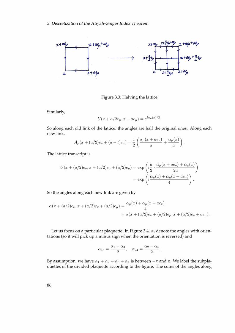
3 Discretization of the Atiyah–Singer Index Theorem
Figure 3.3: Halving the lattice
Similarly,
U(x+ a/2eµ, x+ aeµ) = eiαµ(x)/2.
So along each old link of the lattice, the angles are half the original ones. Along eachnew link,
Aµ(x+ (a/2)eν + (a− t)eµ) =1
2
(αµ(x+ aeν)
a+αµ(x)
a
).
The lattice transcript is
U(x+ (a/2)eν , x+ (a/2)eν + (a/2)eµ) = exp
(ia
2· αµ(x+ aeν) + αµ(x)
2a
)= exp
(iαµ(x) + αµ(x+ aeν)
4
).
So the angles along each new link are given by
α(x+ (a/2)eν , x+ (a/2)eν + (a/2)eµ) =αµ(x) + αµ(x+ aeν)
4= α(x+ (a/2)eν + (a/2)eµ, x+ (a/2)eν + aeµ).
Let us focus on a particular plaquette. In Figure 3.4, αi denote the angles with orien-tations (so it will pick up a minus sign when the orientation is reversed) and
α13 =α1 − α3
2, α24 =
α2 − α4
2.
By assumption, we have α1 + α2 + α3 + α4 is between −π and π. We label the subpla-quettes of the divided plaquette according to the figure. The sums of the angles along
86
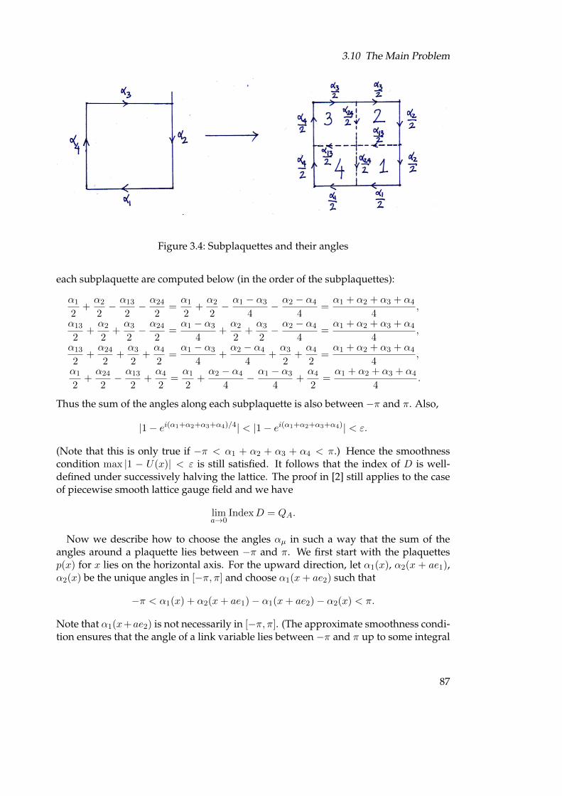
3.10 The Main Problem
Figure 3.4: Subplaquettes and their angles
each subplaquette are computed below (in the order of the subplaquettes):
α1
2+α2
2− α13
2− α24
2=α1
2+α2
2− α1 − α3
4− α2 − α4
4=α1 + α2 + α3 + α4
4,
α13
2+α2
2+α3
2− α24
2=α1 − α3
4+α2
2+α3
2− α2 − α4
4=α1 + α2 + α3 + α4
4,
α13
2+α24
2+α3
2+α4
2=α1 − α3
4+α2 − α4
4+α3
2+α4
2=α1 + α2 + α3 + α4
4,
α1
2+α24
2− α13
2+α4
2=α1
2+α2 − α4
4− α1 − α3
4+α4
2=α1 + α2 + α3 + α4
4.
Thus the sum of the angles along each subplaquette is also between −π and π. Also,
|1− ei(α1+α2+α3+α4)/4| < |1− ei(α1+α2+α3+α4)| < ε.
(Note that this is only true if −π < α1 + α2 + α3 + α4 < π.) Hence the smoothnesscondition max |1 − U(x)| < ε is still satisfied. It follows that the index of D is well-defined under successively halving the lattice. The proof in [2] still applies to the caseof piecewise smooth lattice gauge field and we have
lima→0
IndexD = QA.
Now we describe how to choose the angles αµ in such a way that the sum of theangles around a plaquette lies between −π and π. We first start with the plaquettesp(x) for x lies on the horizontal axis. For the upward direction, let α1(x), α2(x + ae1),α2(x) be the unique angles in [−π, π] and choose α1(x+ ae2) such that
−π < α1(x) + α2(x+ ae1)− α1(x+ ae2)− α2(x) < π.
Note that α1(x+ae2) is not necessarily in [−π, π]. (The approximate smoothness condi-tion ensures that the angle of a link variable lies between −π and π up to some integral
87
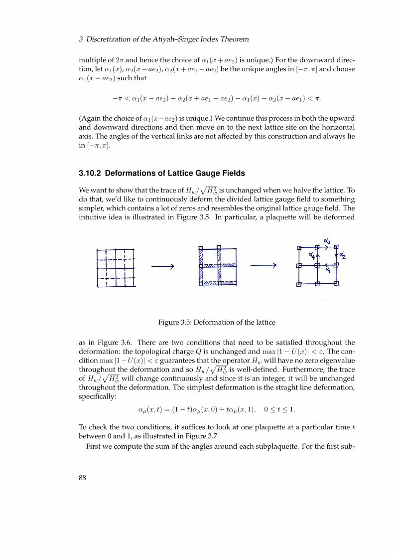
3 Discretization of the Atiyah–Singer Index Theorem
multiple of 2π and hence the choice of α1(x+ ae2) is unique.) For the downward direc-tion, let α1(x), α2(x− ae2), α2(x+ ae1− ae2) be the unique angles in [−π, π] and chooseα1(x− ae2) such that
−π < α1(x− ae2) + α2(x+ ae1 − ae2)− α1(x)− α2(x− ae1) < π.
(Again the choice of α1(x−ae2) is unique.) We continue this process in both the upwardand downward directions and then move on to the next lattice site on the horizontalaxis. The angles of the vertical links are not affected by this construction and always liein [−π, π].
3.10.2 Deformations of Lattice Gauge Fields
We want to show that the trace ofHw/√H2w is unchanged when we halve the lattice. To
do that, we’d like to continuously deform the divided lattice gauge field to somethingsimpler, which contains a lot of zeros and resembles the original lattice gauge field. Theintuitive idea is illustrated in Figure 3.5. In particular, a plaquette will be deformed
Figure 3.5: Deformation of the lattice
as in Figure 3.6. There are two conditions that need to be satisfied throughout thedeformation: the topological charge Q is unchanged and max |1 − U(x)| < ε. The con-dition max |1−U(x)| < ε guarantees that the operator Hw will have no zero eigenvaluethroughout the deformation and so Hw/
√H2w is well-defined. Furthermore, the trace
of Hw/√H2w will change continuously and since it is an integer, it will be unchanged
throughout the deformation. The simplest deformation is the straght line deformation,specifically:
αµ(x, t) = (1− t)αµ(x, 0) + tαµ(x, 1), 0 ≤ t ≤ 1.
To check the two conditions, it suffices to look at one plaquette at a particular time tbetween 0 and 1, as illustrated in Figure 3.7.
First we compute the sum of the angles around each subplaquette. For the first sub-
88
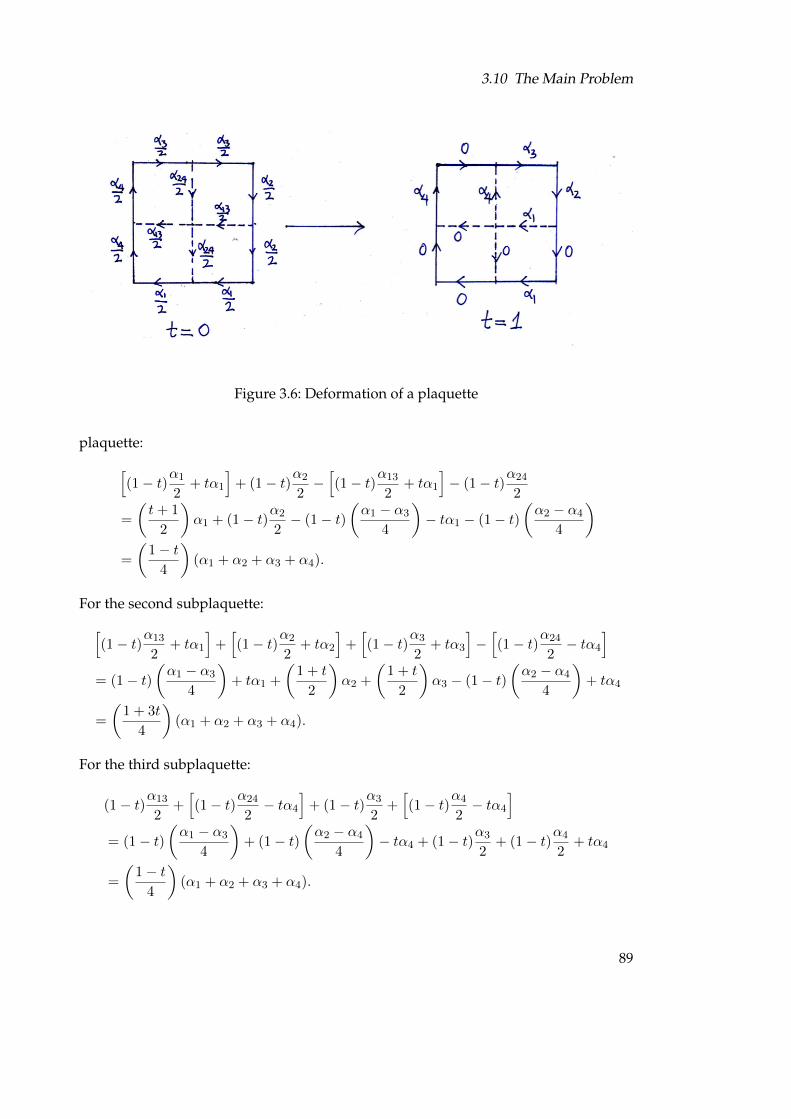
3.10 The Main Problem
Figure 3.6: Deformation of a plaquette
plaquette:[(1− t)α1
2+ tα1
]+ (1− t)α2
2−[(1− t)α13
2+ tα1
]− (1− t)α24
2
=
(t+ 1
2
)α1 + (1− t)α2
2− (1− t)
(α1 − α3
4
)− tα1 − (1− t)
(α2 − α4
4
)=
(1− t
4
)(α1 + α2 + α3 + α4).
For the second subplaquette:[(1− t)α13
2+ tα1
]+[(1− t)α2
2+ tα2
]+[(1− t)α3
2+ tα3
]−[(1− t)α24
2− tα4
]= (1− t)
(α1 − α3
4
)+ tα1 +
(1 + t
2
)α2 +
(1 + t
2
)α3 − (1− t)
(α2 − α4
4
)+ tα4
=
(1 + 3t
4
)(α1 + α2 + α3 + α4).
For the third subplaquette:
(1− t)α13
2+[(1− t)α24
2− tα4
]+ (1− t)α3
2+[(1− t)α4
2− tα4
]= (1− t)
(α1 − α3
4
)+ (1− t)
(α2 − α4
4
)− tα4 + (1− t)α3
2+ (1− t)α4
2+ tα4
=
(1− t
4
)(α1 + α2 + α3 + α4).
89
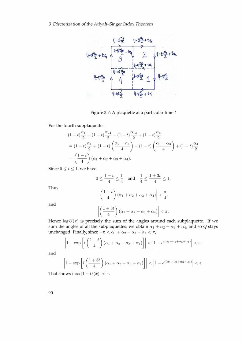
3 Discretization of the Atiyah–Singer Index Theorem
Figure 3.7: A plaquette at a particular time t
For the fourth subplaquette:
(1− t)α1
2+ (1− t)α24
2− (1− t)α13
2+ (1− t)α4
2
= (1− t)α1
2+ (1− t)
(α2 − α4
4
)− (1− t)
(α1 − α3
4
)+ (1− t)α4
2
=
(1− t
4
)(α1 + α2 + α3 + α4).
Since 0 ≤ t ≤ 1, we have
0 ≤ 1− t4≤ 1
4and
1
4≤ 1 + 3t
4≤ 1.
Thus ∣∣∣∣(1− t4
)(α1 + α2 + α3 + α4)
∣∣∣∣ < π
4,
and ∣∣∣∣(1 + 3t
4
)(α1 + α2 + α3 + α4)
∣∣∣∣ < π.
Hence logU(x) is precisely the sum of the angles around each subplaquette. If wesum the angles of all the subplaquettes, we obtain α1 + α2 + α3 + α4, and so Q staysunchanged. Finally, since −π < α1 + α2 + α3 + α4 < π,∣∣∣∣1− exp
[i
(1− t
4
)(α1 + α2 + α3 + α4)
]∣∣∣∣ < ∣∣∣1− ei(α1+α2+α3+α4)∣∣∣ < ε,
and ∣∣∣∣1− exp
[i
(1 + 3t
4
)(α1 + α2 + α3 + α4)
]∣∣∣∣ < ∣∣∣1− ei(α1+α2+α3+α4)∣∣∣ < ε.
That shows max |1− U(x)| < ε.
90
3.10 The Main Problem
3.10.3 Index Density
Consider the vector space W of functions from the lattice sites to C with periodicboundary condition and A is an operator on it. We know that an orthonormal basisfor W is given by
β =
{1
aδx : x ∈ Γ
}.
If ψ is an element in W , then it can be expressed as
ψ =∑x∈Γ
aψ(x)δxa.
Thus with respect to β, ψ is represented by a vector whose entries are the values ofψ on the lattice sites in Γ. Let A be the matrix representation of A with respect to β.The entries of A can be labelled by the lattice sites and we let A(x, y) denote 1/a2 the(x, y)-entry of A, i.e.,
A(x, y) =1
a2
⟨Aδya,δxa
⟩.
With that notation, we have
(Aψ)(x) = a2∑y∈Γ
A(x, y)ψ(y), x ∈ Γ.
In our case, ψ is a function from the lattice sites to C2. The basis element δx acquiresanother index i
δix = δxei.
By representing A with respect to the new basis, taken into account the new index, weobtain the same formula
(Aψ)(x) = a2∑y∈Γ
A(x, y)ψ(y), x ∈ Γ.
However in this case A(x, y) is a 2× 2 matrix, i.e., an operator on C2. The (i, j)-entry ofthat matrix is given by
A(x, y)ij =1
a2
⟨Aδjya,δixa
⟩.
The trace of A is obtained by taking the sum of the diagonal entries of A, thus
trA = a2∑x∈Γ
trA(x, x).
Recall that the index of D is given by
Index (D)lattice = −1
2tr
Hw(1/a)√H2w(1/a)
= −1
2a2∑x∈Γ
trHw(1/a)√H2w(1/a)
(x, x).
91
3 Discretization of the Atiyah–Singer Index Theorem
The term
q(x) = −1
2tr
Hw(1/a)√H2w(1/a)
(x, x)
is called an index density. The formula for the index becomes
Index (D) = a2∑x∈Γ
q(x).
The reason we want to express the index in this form is because in the continuum, theindex (which is the same as the topological charge) is
1
2π
∫[0,1]2
F12(x1, x2)dx1dx2.
If we define the continuum index density as
qA(x) =1
2πF12(x),
then the continuum index becomes
lima→0
a2∑x∈Γ
qA(x),
which resembles our formula in the discrete case.
3.10.4 Computational Approaches
In this subsection we present some computational approaches to the index of D. Sincethe index involves 1/
√H2w, the key is to find different ways to express the inverse
square root of H2w into a more manageable form. (In a computer, we can compute the
eigenvalues of Hw for certain gauge fields approximately.) We’re going to discuss twoways to represent the inverse square root, one via integral representation and one viaLegendre polynomials (Section 1.4).
We first talk about integration of matrices. Consider a family of operators {A(x)} onV depending smoothly on x, i.e., if we choose a basis for V , then {A(x)} becomes a fam-ily of matrices and each entry is a smooth function in x. This definition of smoothnessdoesn’t depend on the choice of basis since if we change the basis, then each matrixA(x) becomes Q−1A(x)Q, where Q is some invertible matrix not depending on x. Wedefine ∫
A(x)dx : =
∫A(x)dx,
where the integral on the right hand side is applied to each entry of the matrix A(x).Again this definition doesn’t depend on the choice of basis since it can be shown easilythat ∫
Q−1A(x)Qdx = Q−1
(∫A(x)dx
)Q
for some invertible matrix Q not depending on x.
92
3.10 The Main Problem
Proposition 3.15. LetA be a strictly positive operator (the eigenvalues are positive), the inversesquare root A−1/2 has the following integral representation
A−1/2 =2
π
∫ ∞0
(A+ t2)−1dt.
Proof. Let (v1, ..., vn) is an orthonormal basis for V consisting of eigenvalues of A, i.e.,
Avi = λivi, i = 1, ..., n.
The eigenvalues of (A+ t2)−1 are smooth functions of t:
(λi + t2)−1, i = 1, ..., n.
Thus to show the equality, it suffices to show that
1√λ
=2
π
∫ ∞0
dt
λ+ t2.
We evaluate the integral of the right hand side:∫ ∞0
dt
t2 + λ=
∫ ∞0
dt
λ
((t√λ
)2+ 1
)
=1√λ
∫ ∞0
d(
t√λ
)(
t√λ
)2+ 1
=1√λ
arctan
(t√λ
)∣∣∣∣∞0
=π
2√λ.
Now we present another way to express 1/√H2w, via the Legendre polynomials. Re-
call that the Legendre polynomials have the following generating function:
1√x2 − 2tx+ 1
=∞∑n=0
Pn(t)xn, |x| < 1, |t| ≤ 1.
From Section 3.6 we know that there exists a constant u independent of the choice ofthe gauge field such that
H2w ≥ u > 0
provided the gauge fields satisfy the approximate smoothness condition
maxx,µ,ν|1− U(x, µ, ν)| < ε
93
3 Discretization of the Atiyah–Singer Index Theorem
for some appropriately chosen ε > 0. (Here the inequality of Hw means the corre-sponding inequalities for its eigenvalues.) The operator Hw also has an upper boundindependent of the gauge fields as follows:
‖Hw‖ =
∥∥∥∥γ3
(Dw −
1
a
)∥∥∥∥ ≤∑ ‖∇µ‖+a
2
∑‖∆ν‖+
1
a=
9
a.
(Consider Section 3.6 for the bounds used for ∇ and ∆.) Let v > u be an upper boundfor H2
w and consider the following operator
T =1
v − u(v + u− 2H2
w).
The operator T is self-adjoint. If λ is an eigenvalue of H2w, then
u ≤ λ ≤ v.
Therefore,u− v ≤ v + u− 2λ ≤ v − u.
Thus the eigenvalues of T lies in [−1, 1]. It follows that
1√x2 − 2xT + 1
=
∞∑n=0
xnPn(T ), |x| < 1. (3.7)
(This is true because T is hermitian and the equality holds for all eigenvalues of T .) Theexpansion is true for any |x| < 1 and so we can choose x to simplify it. Since
v + u
v − u> 1,
there exists a unique θ > 0 such that
v + u
v − u= cosh θ =
eθ + e−θ
2.
Put x = e−θ, then clearly |x| < 1 and we have
x2 − 2x
(v + u
v − u
)+ 1 = e−2θ − 2e−θ
(eθ + e−θ
2
)+ 1 = 0.
With that choice of x, the expression on the left hand side of (3.7) becomes
x2 − 2xT + 1 = x2 − 2x1
v − u(v + u− 2H2
w) + 1
= x2 − 2x
(v + u
v − u
)+ 1 +
4x
v − uH2w
=4x
v − uH2w.
We finally obtain an expansion of 1/√H2w in terms of the Legendre polynomials:
1√H2w
=
√4x
v − u
∞∑n=0
xnPn(T ).
94
Bibliography
[1] David H. Adams. Discrete version of atiyah–singer index theory from lattice gaugetheory.
[2] David H. Adams. On the continuum limit of fermionic topological charge in latticegauge theory. Journal of Mathematical Physics, 42(12), 2001.
[3] David H. Adams. Axial anomaly and topological charge in lattice gauge theorywith overlap dirac operator. Annals Phys, 296:131–151, 2002.
[4] David H. Adams. General bounds on the wilson-dirac operator. Physics Review D,68, 2003.
[5] Sheldon Axler. Linear Algebra Done Right. Springer, second edition, 1997.
[6] John Baez and Javier P. Muniain. Gauge Fields, Knots and Gravity. World Scientific,1994.
[7] Keith Conrad. Computing the norm of a matrix.
[8] R. Courant and D. Hilbert. Method of Mathematical Physics Volume 1. IntersciencePublishers, INC., New York, 1952.
[9] C. Gattringer and C.B. Lang. Quantum Chromodynamics on the Lattice. Springer,2010.
[10] I. S. Gradshteyn and I. M. Ryzhik. Table of Integrals, Series and Products. AcademicPress, seventh edition, 2007.
[11] Pilar Hernandez, Karl Jansen, and Martin Luscher. Locality properties of neu-berger’s lattice dirac operator. Nuclear Physics B, 552:363–378, 1999.
[12] Nicholas J. Higham. Functions of Matrices Theory and Computation. Society for In-dustrial and Applied Mathematics, 2008.
[13] Tosio Kato. Perturbation Theory for Linear Operators. Springer, 1995.
[14] Erwin Kreyszig. Introductory Functional Analysis with Applications. John Wiley andSons, 1989.
[15] Paul Loya. An introductory course in differential geometry and the atiyah–singerindex theorem, .
95
Bibliography
[16] Paul Loya. The atiyah–singer index theorem 1 and 2, .
[17] Rajamani Narayanan. Spectrum of the hermitian wilson dirac operator. NuclearPhysics B (Proc. Suppl.), 73:86–91, 1999.
[18] Andriy Petrashyk. Influence of topology on fermionic zero-modes in lattice gaugetheory. Honour project, School of Physical and Mathematical Sciences (NTU),2010.
[19] John Rognes. On the atiyah–singer index theorem.
[20] Walter Rudin. Principles of Mathematical Analysis. McGraw-Hill, third edition, 1976.
[21] Agustinus Peter Sahanggamu. Generating functions and their applications.
[22] Ng Wen Zheng Terence. The atiyah–singer index theorem in a discrete setting.Honour project, School of Physical and Mathematical Sciences (NTU), 2010.
[23] E. T. Whittaker and G. N. Watson. A Course of Modern Analysis. Cambridge Uni-versity Press, fourth edition, 1963.
96