RURAL ECONOMY

New Instruments for Co-ordination and Risk Sharing

Within the Canadian Beef Industry

James Unterschultz

Project Report 00-04 AARI Project 96H070

Project Report

Department of Rural Economy Faculty of Agriculture, Forestry and Home Economics University of Alberta Edmonton, Canada

II

New Instruments for Co-ordination and Risk Sharing

Within the Canadian Beef Industry

James Unterschultz Principal Researcher

Sumbitted May 12, 2000

Project Report 00-04

AARI Project 96H070

The principal researcher is, Associate Professor, Department of Rural Economy, University of Alberta, Edmonton, Alberta. Copyright 2000 by J. Unterschultz. All rights reserved. Readers may make verbatim copies of this document for non-commercial purposes by any means, provided that this copyright notice appears on all such copies.

III

N E W I N S T R U M E N T S F O R C O - O R D I N AT I O N A N D R I S K S H A R I N G W I T H I N T H E C A N A D I A N B E E F

I N D U S T R Y

James Unterschultz, Darren Chase, Russell Tronstad, Kojo Akabua and Nelson Bungi

EXECUTIVE SUMMARY

The Canadian beef industry has stated objectives of improving beef quality and consumer satisfaction while reducing unit costs of production. Suggested methods for achieving these goals include working towards value based marketing and improved information flows between different market levels through systems such as a birth to plate information system. These initiatives are designed to provide a more direct link between consumer product needs and breeding and management decisions at the farm level. The industrialization of agriculture has introduced a number of changes to the structure of livestock production (Boehlje 1996); from vertical integration (arrangements such as packers feeding cattle) and forward contracting to increasing concentration (of packers and feedlots) within the marketing structure. In the past emphasis was placed on marketing what was produced. Today the challenge is to find value added markets for products. This has promoted changes to the way in which beef and beef products are priced and sold. Vertical coordination has been suggested as a means of dealing with such pricing aspects and information transmission. Grid pricing for finished cattle is also proposed another method to improve the industry by providing more information to all levels of the industry. This research evaluates several areas in coordination, pricing and risk for cattle. These areas are: • Introduction to theory of vertical coordination • Risk tools to manage market risk in the cattle industry • Sources of risk in the cattle industry • Review of the Alberta beef cattle industry structure • Level of use of risk tools by the cow-calf sector in Alberta • Math models and evaluation for new derivative tools • Evaluation of Value-Based-Marketing using Alberta cattle research data • Case studies in vertical coordination and managing risk This report addresses the issues in risk and vertical co-ordination in the beef industry. It provides information, new research and suggestions for moving the beef industry in Alberta forward. The original research proposal planned to develop math models and pricing contracts that can be used by cow-calf, backgrounder, processors and feedlot

IV

sectors. These models are developed and simulated but not extended. Preliminary research showed them to be useful but the use would be limited. Traditional risk tools would be more relevant in most cases. Instead, further risk management might be achieved by evaluating different marketing channels for the beef industry through more co-ordination and the risks surrounding grid pricing. These extensions were pursued in this study. Theory Consumer taste and behavior has triggered the production of consumer-driven food products (through vertical coordination), to fit with the new consumer demand. The food industry in general is offering a wider variety of food products of consistently higher quality. But some economists also contend that although consumer preference is a factor that promotes vertical coordination, market power and especially transaction costs are the driving forces behind it. There is an extensive theory surrounding vertical coordination and two branches are briefly examined in this report. A number of standard risk tools, derivatives, exist. Futures contracts, basis, options and forward contracts are risk tools. These can be used to build a number of different risk management strategies for price risk. Sources of Cattle Risk Market price risk is one major source of risk. This can be composed of overall price risk, basis risk and currency risk. The conversion of live cattle into meat introduces two more components of variability into the equation; yield and grade risk. Yield risk reflects the conversion from pounds of live animal into pounds of beef in the "carcass equivalent". Quantifying the degree of risk faced by cattle feeders and processors and determining the effectiveness of the risk management tools is a task of identifying the type of risk, who currently bears this risk, and determining whether there are mutually advantageous ways of transferring this risk. Grid pricing or related concepts of Value-Based-Marketing/Value-Based-Pricing (VBM, VBP) are similar concepts considered for managing yield and quality risk. Derivative Use in the Cow-Calf Sector AAFRD surveyed over 1700 cow-calf producers in Alberta in 1999. The two main ways cow-calf producer market calves are selling as weaned and retaining ownership. The most preferred marketing method for those who sold as weaned is the ring auction method. The most popular marketing method adopted if ownership is retained is background and plan to sell to feedlots. Forwards, futures and options contracts hedging strategies are not popular among farmers in the Alberta and their use by the cow-calf sector are almost zero. Finally, most farmers are not currently receiving carcass data. However, most will be interested in receiving these data which is important if the industry is to move beyond value-based-pricing. Standard market based risk

V

management tools are not used by the cow-calf sector. This suggests that alternative arrangements will be required to manage market risk in a marketing system that uses more vertical coordination. New Derivative Risk Instruments The basic math models for window contracts and spread contracts are evaluated. Window contracts are a new and growing over the counter price risk tool in the hog industry used to set floor and ceiling prices. Applications to the beef industry would use similar mathematical and numerical models. These instruments provide a mechanism which protects users partly from decreasing market prices but provides greater flexibility in gaining from upward market moves than hedging or forward contracts. Window contracts can be priced as a portfolio of long European puts and short European calls using special combinations of standard option models. They provide a floor price and a ceiling price. Short-term window contracts are not without their problems. Selection of the price floor and ceiling is not a trivial issue. The relationship between futures prices and production costs are such that a short-term window contract that will guarantee no losses cannot always be offered. The window widths vary extensively over time, the price floor moves with changing price conditions, and the risk properties of the contract change with this variation. Thus, short-term window contracts produce more volatile price protection than their long-term -- several years in length -- counter parts. Commodity pricing contracts are being used for managing risk in long term producer-processor contracting relationships. These contracts include long-term window contracts and cost plus contracts. These contracts can be also be decomposed into portfolios of puts and calls. With the cost-plus price contract the producer buys a spread between input prices and output price and sells a spread between input prices plus cost and output prices. These spread alternatives can be valued as puts and calls on the spread. In theory these puts and calls can be valued. However, several valuation constraints exist with long-term contracts that are lessor issues with shorter term contracts. A key input or assumption to value these contracts is the stochastic process used for the price distribution. Window and spread contract values were simulated assuming either a random walk stochastic process or a mean reverting stochastic price process. A random walk process, a non-stationary series, can be difficult to distinguish from a stationary process, a mean reverting series. The different assumptions on the stochastic process have very different implications on the option values contained in window contracts and cost plus contracts. Mean reverting processes, where the mean is correctly identified, lead to lower valued implied options in both window and spread contracts. Different strike prices may be required for different times to maturity if the value of floor price (put option) is to equal the value of the ceiling price (call option) for window contracts. The floor and ceiling prices for window contracts and the cost plus portion of spread contracts

VI

need to change with the expected delivery date. Window contracts can be fairly priced at the opening of the contract, however under the random walk hypothesis, it is highly likely that one party will end up substantially ahead. With a mean reverting process, if the mean is correctly identified and the floor and ceiling prices correctly placed then the window contract appear to hold lower risk. Identifying the mean can be very difficult. Ad hoc adjustments to the contract may be required to keep the contract "fair" to all parties. These types of long term contracts may have relatively low use by the cattle industry. However, these models could be used to help set initial prices if parties enter into long term pricing arrangements. The arrangements will need to be periodically reviewed to make sure that both parties are satisfied with the arrangement. Alberta Grid Pricing Study Data from two Alberta research trials are used to examine grid pricing for finished cattle. The pricing grid used in this analysis is a quality grid that rewards top quality animals within a specified weight range. Over- and under-weight carcasses are discounted. The variation in animal value in this study is based on variations in quantity (weight and dressing percentage), quality (lean meat yield and marbling grades), and the variation in prices offered at sale. A model was used to simulate prices for live weight, dressed weight, and grade and yield revenues using data from two research trials in Alberta. The most notable difference between the two trials is the opposite direction returns take when cattle are individually priced on a grid. Steers on feed in Trial 1 were larger yearlings that dressed out at much higher end-weights. The grid used in this analysis would have produced lower average returns compared to either a live weight or dressed weight pricing method. The steers and heifers placed on feed in Trial 2 were in general much lighter calves that dressed out to lighter end-weights. Weight and the presence of “out-type” steers and heifers largely influence the variability of pen revenue when price is set according to a visual representation of the average carcass traits of a pen of cattle. In a grid that rewards for quality the results are consistent with expectations. The “quality” heifers gained from grid pricing while the “weight” steers were penalized. Looking at the distribution of these returns, cattle in the first trial were penalized for overweight carcasses when priced on a grid schedule. A large percentage of cattle were outside the target weight parameters and were subsequently discounted. By examining only the gross revenue generated by the three pricing methods, live weight, dressed weight or grid, the question of overall profitability still remains. Although these Trial 1cattle were “net” discounts on a grid it is entirely feasible that the additional weight generated by these carcasses may result in lower profits for a live and dressed weight pricing system. If the incentive, or disincentive in this case, is large

VII

enough then additional pounds may well prove to generate even less profits. Feeding costs and the impact on quality and yield grades are key inputs to determining a relationship between weight gain and grid performance. While packers ostensibly reward feedlot operators for removing the degree of uncertainty surrounding their final product, pricing the characteristics of individual carcasses means greater variability in market price to cattle feeders as compared to an average price – instead of one price there are many prices.. The results here (in the study) indicate that while individual animal values may be more volatile under the grid pricing system, the pattern is not consistent across all trials. However, one should not expect the variation in total pen values received over numerous pens to be any different under the pricing systems. Different grids for different points of the year reflecting the type of cattle in the market may be required. Profitability in the Alberta cattle feeding sector is influenced by many factors. Carcass merit has been examined as one of those factors affecting feedlot revenue and revenue variability. Determining carcass merit also emphasizes a shift away from average pen-based pricing to valuing slaughter cattle on an individual animal basis. Methods of pricing slaughter cattle on an individual carcass basis can also provide an economic signal to cattle producers about preferred carcass characteristics. Price plays a dual role – establishing transaction value between packers and cattle feeders as well as conveying important information about consumers preferences for different quality beef products. Results from the Alberta study indicate that grid pricing is an effective method for transferring information about animal value from the packer to the feedlot operator. Grid pricing does not always mean the highest average pen or animal revenue. Trying to match cattle to the pricing grid, however can still be beneficial from a short-term revenue perspective for individual cattle feeders. The key to success of value-based marketing programs is to use the economic signals created by the grid price to effect longer-term improvements in beef quality characteristics through beef cattle genetics and management. One topic that warrants further examination is the issue of basis risk. Valuing cattle on the merit of individual carcasses transfers the risk of animal quality (yield and quality grades) from the packer to the seller. Graff and Schroeder (1998) propose that this transfer of risk adds a component to basis risk; transaction price variability. While the local cash price may be an important element of the base grid price, cattle sold on a grid formula are penalized and rewarded for specific carcass traits above and below the base. The authors found that basis variability increases under grid pricing primarily due to the uncertainty surrounding animal quality, carcass dressing percentages, and variability in local packer premiums and discounts. This is significant in trying to first, assess the difference in pricing methods, and second, in trying to forecast basis levels as part of a risk management program.

VIII

Case Studies on LCC, SLB, Ralphs and WF Moving the beef industry toward a marketing system that will provide better tenderness, consistency, and flavorful meat is a formidable challenge. This challenge is most noteworthy given that two pieces of meat with the same “label” at most retail counters could easily have come from strikingly different genetic and management paths. Lamb and Beshear describe a) pricing innovations, b) producer cooperatives and marketing alliances, and c) supply chains as three different forms of “vertical integration” that might eventually prevail for the beef industry to address their quality challenge. Schroeder, et al. also provides a summary of research issues that agricultural economists can address for this beef industry issue. The conclusions of these two studies are integrated into the insights we obtained from our seedstock, feedlot, packer, and retail companies to formulate the following industry action steps and policy considerations related to value-based-pricing The companies contacted or reviewed provide insights into the major challenges facing the beef industry and potential ways to manage these challenges. Leachman Cattle Co. (LCC), a large US based beef seedstock company, provides insights on the genetic side of the beef quality and production equation. Western Feedlots (WF), a large feedlot company in Western Canada is implementing a value based pricing program for both WF and their custom feeder clients, which provides insights on reducing animal variability. Sun Land Beef (SLB), a beef slaughter and packinghouse, provides insights on everything from feedlot contracting to the inputs needed to produce a wholesale product that is uniform, safe, and competitively priced. Ralphs Grocery Co., a major California supermarket chain, has had a successful branded beef product since 1992 using Holstein genetics, contract feeding through SLB, and SLB as their main processor. The following are key conclusions from the case studies. Derived Demand Education. If producers wish to participate in any value-enhancing attributes of beef they need to recognize that their derived demand will only improve if they participate in adding product value to the final consumer. More education is needed for producers to better understand the derived demand process. Also, it is important to note that gains can be realized in every sector from producing and developing the market for a better beef product. Changing Beef Quality. While several studies have used aggregate data to analyze the issue of “changing consumer demand for beef” (e.g., Eales and Unnevehr, 1993, Moschini and Meilke), no studies have looked at the “changing palatability of beef for consumers.” Admittedly, secondary data are not readily available for even proxies on beef quality characteristics over time. But Ralphs has listened to their consumers on a regular basis through time, albeit informal. Ralphs perceived that “health consciousness” (e.g., Chavas) and “convenience” (e.g., Eales and Unnevehr, 1988) were not significant factors in contributing to any decline in the demand for beef. Rather, the most significant

IX

factor that can be attributed to any decline in the demand for beef has precipitated from a steady decline in beef palatability and consistency. Ralphs concluded that these quality declines have largely been driven by an increase of “exotics” in breed mixes that started in the early 1950’s. In 1950, less than ten breeds of purebred cattle were used for converting grain into beef and the number of breeds has increased at least ten-fold since then. Given that most commercial herds are a mixture of several breeds, the genetic lineage that comprises the current beef herd probably exceeds the number of cow-calf producers. LCC also feels that breeding has largely occurred without a plan since over two-thirds of all cattle miss the target of at least a Choice grade and Yield 2 grade or better. More primary research that quantifies the quality of beef, much like the National Tenderness Survey, should be undertaken by the beef industry. Demand Chain Communication. As noted by Schroeder et al., there is a need for more information regarding consumers’ willingness to pay for meat products that are more customized to match their demand. While more formal research regarding consumer demand for different beef attributes would undoubtedly be very helpful, it is interesting to note that Ralphs did not conduct any formal demand study before they launched their program. Their program was largely undertaken as a response to the complaints and comments that they received from their consumers. The beef industry could easily set up a web site that would enable consumers to voice what they dislike and like about their beef purchases. This feedback could then be used to develop a “knowledge data base” that would help target beef attributes that should be improved by region. Clearly, the beef industry would be better served by paying more attention to the consumer than trying to change grading standards. More Targeted Genetic and Management Paths. The supply chain structure and producer marketing alliances described by Lamb and Beshear are essentially two forms of narrowing genetic and management paths. Holsteins were the only breed Ralphs found available to supply consistent, acceptable quality, and steady supplies of fresh beef throughout the year. While programs like Certified Angus Beef, Farmland Supreme, and Certified Hereford Beef narrow genetic diversity, their genetic requirements are still rather loosely defined and limited. A requirement of 50 percent black hides does not even insure that Angus genetics are from top beef quality lineage. Given consumer demand for consistency and palatability, every sector from seedstock to retail should try to come together and establish a few standardized quality targets and acceptable genetic-management paths for those targets. For example, an age limit and percentage ranges for Continental, English, and other characteristics (e.g., maximum percentage of 15 percent Brahma for heat tolerance) could be set before animals could be classed as Tender. With Artificial Insemination, producers could use semen or first generation bulls from 10 to 15 endorsed semen alternatives on approved cows, similar to what LCC does for their cooperators. More objective measurement of meat characteristics is another possibility, but it is doubtful that measurement can account for the same level of quality attributes that could be built into an identity preserved marketing system.

X

Identity Preservation. In addition to building predictable quality and consistency into a consumer product, identity preservation can serve as a valuable tool for tracking food safety problems and the genetic-management path of a piece of beef that a consumer is unsatisfied with. Regional Demand. LCC is developing seedstock so that at least 70 percent of their animals hit the grid target of at least Choice grade and Yield 2 grade or lower. Although this target reflects the higher end of quality for current grading criteria and price premiums, it may not necessarily be the highest value for all consumers. Both Ralphs and SLB indicated that the Southwest is more of a Select than Choice market. The Select grade from properly fed and tender beef has the highest value for consumers in the Southwest. Research related to a better understanding of regional demand differences should be considered with retail and seedstock sectors sharing a common vision for this effort. Development of a “knowledge data base” described above could be a start for better identifying regional demand differences. Ethnic Markets. Hispanics, African Americans, and Asian Americans currently make up 28 percent of the U.S.’s population and estimates are that they will account for 44.5 percent by 2040 (Silver). Since 1990, overall U.S. buying power has increased 56.7 percent while Hispanic, African American, and Asian American buying power has increased 72.9, 84.4, and 102 percent, respectively (Humphreys, 1998a, 1998b, 1999). Ethnic marketing is much more than translating English labels into another language. More research related to the willingness to pay for attributes in ethnic markets should be considered along with regional demand studies. The Alberta cattle industry must follow these changes in ethnic backgrounds in the United States and take advantage of these opportunities in their largest export market. Vertical Verification. While USDA does all the grading of carcasses at SLB, Ralphs still has one of their employees on the packing line in SLB’s plant making selection decisions. Dietrich noted that this was a key component for making the California Beef program work because it insured credibility of the program to Ralphs. If the beef industry moves to identify more targeted meat products, retailers will need to have input into seedstock selection decisions for any program to work. Likewise, seedstock, cow-calf, and feeder input will be important to insure that production parameters are reasonable. Math Game. As noted by LCC, it takes a lot of cattle to have high selection criteria and a lot of capital to own cows. If an identity preserved marketing system was put in place, a global data base could be established to better identify superior bulls and cow herds for quality and yield attributes targeted. Attributes would need to be objectively measured and compared under similar management conditions. Individuals that participate in such a program should have the opportunity to objectively evaluate how their animals perform relative to other animals from the same geographic region. Although the cost and

XI

logistics of putting together a large scale data base would need to be overcome, the issue deserves attention. Captive Supplies. In the California Beef program, captive supplies were deemed necessary at the beginning to insure that consumers could always go into a Ralphs store and make a repeat brand purchase. Captive supplies were also noted as being important for improving cost efficiencies and profit variability at both the feedlot and packer levels. In the California Beef program, SLB was contracting with feeders for cattle on behalf of Ralphs. A contracted feedlot, SLB, or Ralphs were only required to give a 30 day notice to end their participation in the program. However, cattle in the feeding program prior to a 30 day notice would have to be purchased by Ralphs through SLB, provided they meet contract specifications. A “see how it goes” approach was initiated from the beginning and appears to have worked for the long-term benefit of the relationships involved. When problems come up each partner gains a new perspective for each other’s operation and through joint problem solving each relationship gains a new level of trust and confidence (Kay, 1994). Given the nature of their contracts, one could easily argue that they were more of a vehicle to assure quality and consumer availability rather than exercise market power. When the program was first initiated SLB had to purchase Holsteins outside of what they had contracted for due to bad weather. If the beef industry can identify more targeted genetic and management paths, a “see how it goes” approach between any contracting parties would probably be wise. Pricing / Risk Management. While cow-calf producers often find themselves at the end of the “whipping stick” with feedgraim and fed cattle price fluctuations, the focus of any pricing system should be on economic efficiency rather than income stabilization. While contracts can aid in planning and cost efficiencies, a long-term pricing contract that fails to predict the mean accurately enough will be doomed for failure1. SLB would rather not guess the longer-term trends for the industry. Coming up with the capital to cover losses for when the market steadily moves against SLB’s contracted position is a risk they would rather not take. Technologies and policies can change the underlying structure of an industry rather quickly. Shared ownership at each level, possibly structured like the cooperator arrangements with LCC, appears to have more promise for reducing risk while yielding economic efficiency than contracts that try to predict the long-term mean price for the beef industry. The companies discussed illustrate several key points with respect to beef production-marketing. Genetics, management and the environment are key inputs for the industry. VBP can directly address many of the management issues associated with beef production but the genetic side is only indirectly addressed through VBP. For example, WF provides information back to cooperating cow-calf producers but no genetic program or programs are explicitly tied to these animals. Further the small size of many cooperating cow-calf owners relative to the selection intensity of a seedstock producer like LCC may not be sufficient for these producers to make adequate genetic progress

1 This makes it difficult to write and price long term contracts where price is fixed.

XII

without pooling their numbers. This may require new alliances at the cow-calf level with a seedstock producer or a third party that could identify superior genetics from a pooled population of smaller producer’s herds. Ralphs found desirable palatability and consistent genetics using grain fed Holsteins that would reach slaughter weight in about 13 months. SLB, a packing company, contracts with feedlots for Ralphs to apply feedlot management practices identified for producing quality, consistency, year-round availability, and consumer value. These elements are believed to be key for the consumer loyalty they have developed for their California Beef product. Their branded beef product was tested and re-tested for consumer acceptability before they launched their program. Ralphs selected the Holstein breed from existing genetics largely because of product consistency and the ability to immediately produce year-round supplies. In addition to having a relatively narrow genetic base, a Ralphs employee visually selects animals that will carry their branded beef label. This was identified as a key component for making the California Beef program work. A steady supply of beef through the slaughterhouse was noted by SLB as being very important for keeping their per unit processing costs low. LCC is developing seedstock based on VBP (i.e., targeting over 70 percent of their animals to grade at least Choice with a Yield 2 grade or lower). Their seedstock selection process relies on identifying an elite group of superior outliers from a very large population base. Although LCC considers VBP carcass quality traits (i.e., marbling and yield) for selecting seedstock, limiting their selection process to the quality traits of grid pricing could easily miss key quality attributes. The link between marbling and beef palatability was found to be a poor to moderate link at best by Ralphs for predicting good eating beef. Producing attributes of consistency and tenderness from even a selected sub-set of composites raised in different climatic and range environments presents a formidable challenge to the beef industry. The experience of Ralphs suggests that seedstock selection decisions need to be more focused than just the VBP carcass quality attributes of marbling and yield. Palatability extends beyond grid measures for the consumer and consistency is more than producing animals that hit the same area of the grid. Better information sharing and coordination between seedstock and retail industries could help assure that consumer preferences of palatability and consistency are met while meeting high production standards. In addition, cow-calf, feedlot, and packing industries need to be involved with any genetic plan proposed between seedstock and retail sectors to ensure that management can take full advantage of any genetic-management path targeted. Key conclusions • Theory already exists to explain the potential benefits or reasons for vertical

coordination. • There are a number of risk management tools available to manage price risk in the

beef industry however these tools are not used at the cow-calf sector. This requires

XIII

more research. • Math tools are available to price new derivative risk management products such as

window or spread contracts however long term contracts having a fixed price may be problematic to price in a fair manner.

• Grid pricing (Value-Based-Marketing/Value-Based Pricing) will not necessarily increase producer returns. It will send strong price signals about whether the cattle priced on the grid match that particular grid. Certainly anyone pricing their cattle on a price grid will need to produce cattle designed to meet the grid specifications.

• There is some evidence that the herd origin of the Alberta cattle priced on the grid matters and that some cattle from particular ranches better met the particular grid specifications or graded higher.

• Grid Pricing or (VBP/VBM) may not be enough to move the industry forward to compete with pork and poultry. The industry can manage their cattle to meet certain grid specifications however genetics is a key ingredient in targeting specific beef markets. Genetics is a numbers game and cannot be easily managed by small cow-calf players in the beef industry. Grid Pricing by itself does not directly address the numbers game required for genetic improvement.

XIV

Table Of Contents Executive Summary ...................................................................................................................... III Acknowledgements.................................................................................................................... XIX Abstract ...................................................................................................................................... XIX 1. Introduction..................................................................................................................1 1.1.1. Information Access ......................................................................................................2 1.1.2. Need For Vertical Coordination?................................................................................3 2. Background On Theory................................................................................................5 2.1. Vertical Coordination ..................................................................................................5 2.1.1. Theories Of Vertical Coordination ..............................................................................6 2.2. Measuring Risk And Risk Management Tools............................................................8 2.2.1. Risk Measures ..............................................................................................................8 2.2.2. Government Price Risk Management Instruments ....................................................11 2.2.3. Market Based Derivative Instruments .......................................................................12 2.2.4. Sources Of Beef Cattle Risk .......................................................................................18 2.2.5. Contracts As Alternative Risk Management Tools And Basis For Vertical

Coordination..............................................................................................................22 3. Background On Alberta Cattle Industry ....................................................................23 3.1. Structure Of The Alberta Beef Industry ....................................................................23 3.1.1. Cow-Calf Operations .................................................................................................24 3.1.2. Backgrounding And Finishing Feedlots ....................................................................26 3.1.3. Processing Industry ...................................................................................................28 3.2. Consumers: Domestic And Export Markets ..............................................................28 3.2.1. Globalization Of The Beef Industry ...........................................................................30 3.2.2. Beef Consumption ......................................................................................................30 3.2.3. Beef Demand..............................................................................................................31 3.2.4. Tastes And Preferences..............................................................................................32 3.3. Current Marketing Arrangements ..............................................................................34 3.3.1. Marketing Methods In The Alberta Beef Industry .....................................................35 3.3.2. Issues In Beef Cattle Production And Pricing ...........................................................39 3.3.3. New Marketing Arrangements ...................................................................................43 3.3.4. Alternative Contracting Arrangements For Alberta Feeders....................................44 3.3.5. Summary ....................................................................................................................44 4. State Of Derivative Use By Cow-Calf Sector: Cattle Herd Analysis Survey

Summary Of Marketing Analysis Results .................................................................46 4.1. Farm Types And Farm Operations ............................................................................47 4.2. 1998 Calf Use ...........................................................................................................47 4.3. Marketing Methods Of Weaned Calves.....................................................................47 4.4. Retained Ownership Marketing Methods ..................................................................48 4.5. Use Of Hedging Techniques.....................................................................................48 4.6. Carcass Grading Data ................................................................................................49 4.7. Summary ....................................................................................................................49 4.1. Alberta Beef Cow Calf Audit: Survey Questions Related To Marketing

XV

Practices In 1998........................................................................................................57 5. Pricing Models For Vertical Coordination ................................................................58 5.1. Short-Term Window Contracts..................................................................................58 5.2. Establishing The Price Window For Short Term Contracts ......................................61 5.3. Long Term Window And Spread Contracts ..............................................................62 5.4. Stochastic Processes For Long Term Contracts ........................................................65 5.5. Data Description And Analysis Of Long Term Contracts.........................................66 5.6. Monte Carlo Model Valuation Of Long Term Contracts ..........................................68 5.7. Math Models And Window Contract Conclusions....................................................71 6. Variability In Value-Based Marketing: Risk Sharing In The Alberta Beef

Industry ......................................................................................................................84 6.1. Pricing To Value And Quality Risk...........................................................................84 6.1.1. Carcass Quality .........................................................................................................84 6.1.2. Quality Risk................................................................................................................86 6.1.3. Formula And Grid Pricing ........................................................................................87 6.1.4. Summary ....................................................................................................................87 6.2. Analysis Of Quality Risk ...........................................................................................88 6.2.1. Data Description........................................................................................................89 6.2.2. Analysis And Pricing Methods...................................................................................90 6.2.3. Results ........................................................................................................................93 6.2.4. Grid Performance ....................................................................................................111 6.3. Value-Based Pricing: Conclusions And Recommendations In Alberta ..................113 6.3.1. Implications For Further Research .........................................................................115 7. Case Studies In Vertical Coordination In The Beef Industry ..................................117 7.1. Overview Of Seedstock, Feedlot, Packer, And Retail Companies ..........................118 7.1.1. Leachman Cattle Co. (Lcc) ......................................................................................118 7.1.2. Western Feedlots (Wf) .............................................................................................119 7.1.3. Sun Land Beef (Slb) .................................................................................................119 7.1.4. Ralphs Grocery Co. .................................................................................................119 7.2. Genetics ...................................................................................................................120 7.3. Management And Environment...............................................................................124 7.3.1. Risk Management And Pricing ................................................................................127 7.4. Industry Action And Policy Considerations ............................................................129 8. Conclusions On Managing Risk In Veritical Coordinated Systems........................135 9. References................................................................................................................139 10. Appendix: Canadian Grading System......................................................................149

XVI

Table Of Tables Table 2.1. Alberta Slaughter Steer Basis, Monthly 1989-1997.....................................................14 Table 3.1. Alberta Beef Cow Herd (Census Profile) .....................................................................24 Table 3.2. Alberta Origin Slaughter Cattle & Calves (Census Profile – No. Of Head) ................27 Table 4.1. Breakdown Of Farm Types And Farm Operations According To Regions .................50 Table 4.2. Breakdown Of Use For 1998 Calf By Number Of Respondents According To

Regions. .......................................................................................................................51 Table 4.3. Marketing Methods Of Farmers Who Sold Weaned Calves According To

Regions ........................................................................................................................52 Table 4.4. Marketing Methods Adopted If Ownership Is Retained...............................................53 Table 4.5. Number Of Respondents Adopting Method Of Pre-Pricing Calves, Feeder

Cattle Or Slaughter Cattle In 1998 According To Regions .........................................54 Table 4.6. Number Receiving And Interested In Receiving Carcass Grading Data On

Feeder Cattle That Leave Farm ...................................................................................55 Table 5.1. Simple 90 Day REturns Volatility Estimates For 1987-1997.......................................73 Table 5.2. Simple 90 Day Returns Correlation Estimates For 1987-1997 ....................................73 Table 5.3. Systems Estimates Of Standard Deviations And Correlations Using

Autoregressive Models ................................................................................................74 Table 5.4. Reversion Parameter And Capital Asset Pricing Model Beta Estimates.....................75 Table 6.1. Weekly Carcass Characteristics Of Alberta Steers And Heifers; 1992-98...................86 Table 6.2. Grid Pricing Premiums And Discounts ........................................................................92 Table 6.3. Pricing Grid For Steers .................................................................................................93 Table 6.4. Summary Carcass Characteristics From Trial 1 (10 Pens Of Cattle) ...........................94 Table 6.5. Summary Carcass Characteristics From Trial 2 (34 Pens Of Cattle) ...........................96 Table 6.6. Variation Of Carcass Traits Between Trials.................................................................98 Table 6.7. Summary Of Grid Pricing Method From Trial 1 (10 Pens Of Cattle)..........................99 Table 6.8. Summary Of Grid Pricing Method From Trial 2 (34 Pens Of Cattle)........................100 Table 6.9. Summary Of Pricing Methods From Trial 1 (Live Weight Recorded At Sale)..........101 Table 6.10. Summary Of Pricing Methods From Trial 2 (Live Weight Recorded At Sale)........103 Table 6.11. Test Of Mean Difference Of Pricing Methods .........................................................105 Table 6.12. Summary Of Pricing Methods By Breed Of Cattle ..................................................107 Table 6.13. Summary Of Pricing Methods By Cattle Origin (Live Weight Recorded At

Sale)..........................................................................................................................108

XVII

Table Of Figures Figure 2-1. Classic Hedge Using A Short Futures Position ..........................................................13 Figure 2-2. Alberta Slaughter Cattle Basis Levels, 1993-1997 .....................................................14 Figure 2-3. Payoff From Buying A Put -Or- Writing A Call Option ............................................16 Figure 2-4. Combined Payoff From Buying A Put And Writing A Call Option...........................16 Figure 2-5. Comparison Of Alberta Slaughter Cattle And U.S. Futures Prices ............................19 Figure 2-6. Payoff From Cash Marketing......................................................................................20 Figure 3-1. Five Largest Beef Breeding Herds In North America ................................................23 Figure 3-2. U.S. Beef Cow Inventory – January 1 (Million Head) ...............................................25 Figure 3-3. Canada And Alberta Beef Cow Inventory – January 1 (Million Head)......................25 Figure 3-4. Alberta Fed Cattle Marketings (Steers & Heifers) .....................................................27 Figure 3-5 Major Feeding Areas In North America .....................................................................28 Figure 3-6. Destination Of Alberta’s International Beef Exports, 1996........................................29 Figure 3-7. Alberta Beef Exports Into Far East Markets, 1996.....................................................30 Figure 3-8. Comparison Of Beef Consumption Between Canada And The U.S...........................31 Figure 3-9. Per Capita Consumption Of Red Meat And Poultry, Canada And The U.S...............32 Figure 3-10. Canadian Meat Consumption Patterns......................................................................33 Figure 3-11. U.S. Meat Consumption Patterns ..............................................................................33 Figure 3-12. Weaned/Feeder Calf Marketing Methods .................................................................36 Figure 3-13. Slaughter Cattle Pricing Methods .............................................................................38 Figure 3-14. Total Inspected Slaughter In Alberta ........................................................................39 Figure 3-15. U.S. Beef Cow Inventory And Omaha 500-600 Lb. Steer Price ..............................40 Figure 3-16. Beef Production In Canada .......................................................................................41 Figure 3-17. Trend Of Annual Steer Carcass Weights In Alberta.................................................41 Figure 3-18. Seasonality Of Weekly Alberta Slaughter; Steers And Heifers (1992-1998)...........42 Figure 3-19. Seasonality Of Weekly Carcass Traits; Steers And Heifers (1992-1998) ................43 Figure 5-1. Payoff From Cash Marketing.....................................................................................76 Figure 5-2. Payoff From Buying One Put And Selling One Call ..................................................76 Figure 5-3. Combined Payoff From Put And Call Options ..........................................................77 Figure 5-4. Payoff To Producer Taking A Window Contract (Zero Basis Risk) .........................77 Figure 5-5. Compare Random Walk To Mean Reversion – 10 Years...........................................78 Figure 5-6. Compare Random Walk To Mean Reversion – 40 Years..........................................78 Figure 5-7. Window Contract Example 1 Hogs............................................................................79 Figure 5-8. Window Contract Example 2 Slaughter Cattle ..........................................................79 Figure 5-9. Window Contract Example 3 Feeder Cattle ..............................................................80 Figure 5-10. Window Contract Example 4 Hogs..........................................................................80 Figure 5-11. Window Contract Example 5 Hogs...........................................................................81 Figure 5-12. Call Premiums With Varying Rates Of Mean Reversion ........................................81 Figure 5-13. Spread Contract For Hogs Example 1......................................................................82 Figure 5-14. Spread Contract For Cattle Example 2 ....................................................................82 Figure 5-15. Spread Contract For Cattle: Example 3 ..................................................................83 Figure 6-1. Distribution Of Heifer Quality Grades - Trial 2(A)..................................................109 Figure 6-2. Distribution Of Heifer Quality Grades - Trial 2(B) ..................................................109

XVIII

Figure 6-3. Distribution Of Heifer Yield Grades - Trial 2(A) .....................................................110 Figure 6-4. Distribution Of Heifer Yield Grades - Trial 2(B) .....................................................110 Figure 6-5. Distribution Of Heifer Carcass Weights - Trial 2 .....................................................111 Figure 6-6. Alberta Cash Price, Direct To Packer Sales – Live Weight Basis (1994-1996).......112

XIX

ACKNOWLEDGEMENTS

The author acknowledges the assistance of Darren Chase, Alberta Agriculture Food and Rural Development with the background and analysis of grid pricing, Russell Tronstad, associate specialist, Department of Agricultural and Resource Economics , University of Arizona with the case studies, Kojo Akabua, Research Associate Rural Economy and Associate Professor Canadian University College with the analysis of the AAFRD beef audit data and Nelson Bungi Research Assistant Rural Economy with background research. All names mentioned above are contributing authors to this report. However any final errors or conclusions remain the responsibility of the primary author, Jim Unterschultz. Funding was provided by the Canadian Beef Industry Development Fund. Dr. Frank Novak was the original primary research applicant. This subsequently changed to Dr. Jim Unterschultz. More emphasis was subsequently spent on examining vertical coordination to manage risk.

ABSTRACT

This research evaluates several areas in coordination, pricing and risk in the Alberta beef industry and North America beef industry. This was done through literature review, simulation, analysis of cattle data from two Alberta research trials and case studies. Theory already exists to explain the potential benefits or reasons for vertical coordination. There are a number of risk management tools available to manage price risk in the beef industry however these tools are not used at the cow-calf sector. Math tools are available to price new derivative risk management products such as window or spread contracts however long term contracts having a fixed price may be problematic to price in a fair manner. Grid pricing (Value-Based-Marketing/Value-Based Pricing) will not necessarily increase producer returns. It will send strong price signals about whether the cattle priced on the grid match that particular grid. Certainly anyone pricing their cattle on a price grid will need to produce cattle designed to meet the grid specifications. There is some evidence that the herd origin of the Alberta cattle priced on the grid matters and that some cattle from particular ranches better met the particular grid specifications or graded higher. Grid Pricing or (VBP/VBM) may not be enough to move the industry forward to compete with pork and poultry. The industry can manage their cattle to meet certain grid specifications however genetics is a key ingredient in targeting specific beef markets. Genetics is a numbers game and cannot be easily managed by small cow-calf herd.

1

NEW INSTRUMENTS FOR CO-ORDINATION AND R I S K S H A R I N G W I T H I N T H E C A N A D I A N

B E E F I N D U S T R Y 1. INTRODUCTION

The Canadian beef industry has stated objectives of improving beef quality and consumer satisfaction while reducing unit costs of production. Suggested methods for achieving these goals include working towards value based marketing and improved information flows between different market levels through systems such as a birth to plate information system. These initiatives are designed to provide a more direct link between consumer product needs and breeding and management decisions at the farm level. The stated goals imply the need for vertical market co-ordination which can be achieved in many different ways. Chicken and poultry industries have achieved this co-ordination through various forms of vertical integration. Extreme examples of this include ownership of the entire production chain from genetic seed stock to retail food preparation. This form of co-ordination insures that information produced at the retail level is passed back through the chain, allowing adjustments in any and all parts of the production chain. The beef industry is seeking a system which can capture the benefits arising from this type of co-ordination while retaining a degree of independence between market participants. Co-ordination of market signals from consumers to producers and fair rewards for contributions to value and acceptance of risk are critical for the beef industry to achieve its objectives. This will require an unprecedented level of co-operation and co-ordination in the beef industry. Strategic alliances and long term contracts between producers, processors and retailers will increase in the future. These business relationships will result in the acceptance of various market risks by the contracting parties and require explicit terms for the sharing of market risks and rewards. Indeed, the recent report of the Beef Industry Trade and Development Committee entitled, “A Market Opportunity” outlined the importance to the processing sector of forward pricing and the ability to manage the related price risks. These forward pricing arrangements and risk sharing will only succeed if they are perceived to be fairly and transparently priced. Modern derivatives markets are based on the ability to price the risk arising from these types of arrangements. Indeed, the popularity of derivatives in financial markets lies in their flexibility and low cost (Das 1994). The tools developed by derivatives traders can be adapted to the beef industry to provide objective prices for a wide range of forward contracts which could be used to co-ordinate production and marketing decisions in the beef industry. Specific examples which may be used by the industry include fixed-price and minimum price contracts, contracts priced on market spreads (such as wholesale to live price spread) and risk sharing arrangements such as price window contracts. These can be developed for both short run (less than 12 months) and long run (multiple year) arrangements. Some simple examples of these contracts are being adopted in the hog

2

industry today. As an example, the US industry currently uses price window contracts whereby participants accept all price variability within a specified range but share market moves outside of that range The Alberta beef cattle industry has undergone major structural change in both production and marketing processes towards a more globally oriented system. While much of the attention has been on the rapid expansion of the feeding industry in southern Alberta and the rationalization of the processing industries (CITT 1993; Grier 1998), equally important are the changes in the beef marketing structure. The industrialization of agriculture has introduced a number of changes to the structure of livestock production (Boehlje 1996); from vertical integration (arrangements such as packers feeding cattle) and forward contracting to increasing concentration (of packers and feedlots) within the marketing structure. In the past, emphasis was placed on marketing what was produced. Today the challenge is to find value added markets for products. This has promoted changes to the way in which beef and beef products are priced and sold. Vertical coordination is one means of dealing with pricing aspects and information transmission. These changes have important implications for risk management strategies. Futures markets play a vital role in the process of price discovery and provide an essential tool for risk management. The pricing mechanism for livestock is, in general, complicated by the relative non-storability of the ‘live’ product. Production cycles, time lags in supply response, product seasonality, and the competitiveness among meat products are also significant supply and demand factors. Freer trade has also precipitated the removal of traditional income enhancing and risk reducing government programs. Following the lead of the poultry and pork industries, increased reliance on capital intensive scale economies has made the financial exposure to market risk even more pronounced. A variety of terms are used to describe this movement towards negotiated coordination of production system linkages including “supply chain management” and “captive supply”. The role of information management takes on a new dimension when the links between cattle feeder, processor, and consumer become intertwined.

1.1.1. INFORMATION ACCESS

The ability to gather and evaluate information quickly is spreading throughout the chain as the marketing environment shrinks in ‘spatial’ terms. Processors are starting to test electronic identification systems designed to monitor meat characteristics from the feedlot to the kill floor (Suther 1997). Canada is implementing a cattle identification program commencing Dec 31, 2000 (CCIA 2000). This information is a vital link between the final product and the ability to incorporate such data with the feeding programs and genetics at the producer level. In this sense information has become a valuable commodity, and one which introduces considerable risk. Who bears this risk, and how can it be priced are very legitimate questions?

3

1.1.2. NEED FOR VERTICAL COORDINATION?

Various exchange mechanisms can be found across agricultural commodity groups in Canada. For instance, the supply-managed industries (especially poultry) exhibit relatively tight vertical coordination of marketing channels. Beef cattle and feed grain production in contrast, rely much more on market signals (price) to facilitate coordination. The Mighell and Jones classification of vertical coordination is referred to in a number of papers as a concept for describing ‘alternatives’ for harmonizing the vertical stages in production, processing and marketing (see Barkema, Drabenstott, and Welch 1991; Sporleder 1992). Such alternatives include the price system, vertical integration, contract arrangements, and cooperation. In the traditional ‘open production’ environment, marketing commitments are made only after the production process is complete, that is, once cattle reach slaughter weight. Price performs a dual function of clearing the market and conveying information about end-user preferences. However, this system exposes cattle feeders and processors not only to large swings in the price of beef but also to risks in the availability and quality of slaughter cattle (Barkema, Drabenstott, and Welch 1991). Contracting and vertical integration are two ways to overcome some of the limitations of pure reliance on the price system. Contract arrangements seek to “lock-in” the production or marketing commitment of the cattle feeder in advance and hence, reduce the inherent risks to both parties. Contract production can be as simple as forward pricing or can be more extensive and integrate resources from the processor such as feed, genetics or management. Vertical integration shifts complete control of two or more stages of production to one participant. Numerous studies have examined the increased coordination of vertical linkages within agricultural marketing channels in recent years. In broiler industry contracting accounts for almost 92% of production and is characterized by the processor providing production stock, feed and management support (Aust 1997). Contracting in hog production is around 10% and follows a similar pattern to that of broiler production through feed companies, genetics firms, and processors (Rhodes 1995). Changing consumer demand and technological advances in the food processing industry appear to be the driving forces in this move away from ‘open’ market coordination. Barkema, Drabenstott and Welch (1991) found that 17.5 % of slaughter cattle in the U.S. were produced under some form of feeding/marketing contract compared to 10.0% in 1960. In Canada, roughly 20% of beef cattle are produced under some form of contractual (i.e. forward contracting) arrangement (CITT 1993). Many factors influence the production and marketing systems employed by Alberta cattle feeders. The most obvious factors are profitability and the variability of these net returns.

4

Equally important are issues of capital investment, cash flow, technology, individual risk preferences, and pre-existing attitudes towards the current marketing structure. The decisions facing the cattlemen today are much different than traditional production and marketing choices. In the past many of these decisions reflected a great deal of independence from broader industry issues. Each part of the supply chain tended to view their “job” as complete once control was passed. The growing significance of export markets and global competitiveness has changed much of that. Market coordination has great potential to increase demand by matching the quality and quantity needs of the final consumer with the primary producer (Johnson and Foster 1993). Key to this success, however, is the information flow. Processors, cattle feeders, and cow-calf producers alike need information in order to facilitate sound decisions about production and marketing arrangements. As these new patterns emerge it is essential to analyze the profitability and risk characteristics of these alternatives since the exchange mechanism can impact the sharing of risk (Sporleder 1992). Contracting and vertical integration shortens and clarifies the information flow. Suitable pricing arrangements are also required to evaluate how the risk can be priced or shared between participants. Grid pricing or value-based pricing is suggested as one method of sharing the risks of uncertain animal yield and as a means to pricing individual animal value. Such price signals are an important component in evaluating the success of vertical coordination systems. This research evaluates several areas in coordination, pricing and risk. These areas are: • Introduction to theory of vertical coordination • Risk tools to manage market risk in the cattle industry • Sources of risk in the cattle industry • Review of the Alberta beef cattle industry structure • Level of use of risk tools by the cow-calf sector in Alberta • Math models and evaluation for new derivative tools • Evaluation of Value-Based-Marketing using Alberta cattle research data • Case studies in vertical coordination and managing risk • Overall conclusions. This report addresses the issues in risk and vertical co-ordination in the beef industry. It provides information, new research and suggestions for moving the beef industry in Alberta forward. The original research proposal planned to develop math models and contracts that can be used by cow-calf, backgrounder, processors and feedlot sectors. These models are developed and simulated but not extended. Preliminary research showed them to be useful but the use would be limited. Traditional risk tools would be more relevant in most cases. Instead, further risk management might be achieved by evaluating different marketing channels for the beef industry through more coordination and the risks surrounding grid pricing. These extensions were pursued in this study.

5

2. BACKGROUND ON THEORY

Understanding the key vertical coordination theories, risk theories and risk management tools facilitates understanding how to evaluate vertical coordination and other risk management tools in the Alberta beef industry. Discussions on vertical coordination, risk measures and risk tools follow.

2.1. VERTICAL COORDINATION

The food industry has traditionally operated in a price signaling production system. Martinez (1996) describe this system of production as one in which a firm does not commit to selling its output prior to complete production. This mode of production is typical of the beef industry. But the fact that consumer tastes and preferences are changing is compelling for the industry to make its production system customer-driven by producing products that meet consumer demand. Failure to address this issue may lead to further shrinkage of the industry’s market share because “consumers are now so demanding for detailed product characteristics that it overwhelms the traditional spot market pricing system” (Kinsey, 1994). Vertical coordination2 is given as one solution to addressing consumer preferences. Koontz and Purcell (1997) see production and marketing functions as a joint process which suggests a joint decision making. Stigler (1951) also recognizes that if technically related stages of economic activity are coordinated, it reduces combined costs of these functions. Apart from cost reduction, entrepreneurs also seek minimum variability in revenues. Paul (1974) showed that even in the absence of cost reduction, a firm may still vertically coordinate with an adjacent stage so long as variability of costs and revenues is reduced. New technological developments that allow product differentiation make vertical coordination a feasible system to pursue. Given the constraining nature of the industry’s structure, how can the production process of beef be coordinated? An attempt to address this question is made in the following paragraphs. Coordinating the production process can be carried out through pricing innovations, producer cooperatives and marketing alliances and supply chains. Each option can relay consumer preferences across all or some segments of the production chain. A brief discussion of each option is given below. Another alternative of coordinating activities in the production chain is producer cooperatives and marketing alliances. This option is gaining momentum in the United States. Cooperatives and alliances mainly comprise of cow-calf producers. Their primary 2 Antonovitz et. al. (1996) provide elaborate definitions of vertical integration: “Vertical integration is the consolidation of two successive production processes in which the output of the upstream stage is used as one intermediate input in the downstream stage. The consolidation is such that contractual and open market exchanges between the upstream and downstream firms are eliminated and replaced by internal exchanges within the consolidated firm. As such, vertical integration implies ownership and complete control over neighboring stages of production or distribution.

6

goal is to enhance the flow of information to members to improve quality and reduce production cost (Lamb and Beshear, 1998). Inclusion of the cow-calf segment in information sharing suggests that the cooperatives and alliances option is a vital step toward vertical coordination in the beef industry. The Canadian Angus and Hereford Associations have successfully launched programs where they sell their beef as “specialty products” to retailers (Duckworth, 1999). The certified Angus beef was launched in 1997 and is now found in almost every province in Canada. Since then, sales volumes have tripled (Libby Sally of Canadian Angus Association). The Certified Canadian Hereford retail program was successfully launched ten years ago with Canada Safeway and the association is currently working with restaurants in a bid to include Hereford beef on restaurant menus (DeCorby). A different case study is presented later in this report. The third option that could be used to relay consumer preferences to cow-calf producers is supply chains or vertical integration. In vertical integration one firm controls all stages of production. For practical purposes however this option seems more difficult to achieve given the industry structure described in a later section.

2.1.1. THEORIES OF VERTICAL COORDINATION

Consumer taste and behavior has triggered the production of consumer-driven food products (through vertical coordination), to fit with the new consumer demand. The food industry in general is offering a wider variety of food products of consistently higher quality. But some economists also contend that although consumer preference is a factor that promotes vertical coordination, market power and especially transaction costs are the driving forces behind it. Market Power Market power theories suggest that market power is the motivating force behind vertical coordination. Under this hypothesis, firms gain power by creating barriers to entry at the processing level or exercising price discrimination at the retail level. Through these practices firms maximize profits. But the profits so maximized are of non-competitive nature simply because food processors are often tempted to curtail output which then translates into increased retail prices (Azzam and Wellman, 1992). Martinez, Smith and Zering (1997) indicate that apparent barriers to entry in the processing sectors for the pork industry in the United States, suggest that vertical coordination between hog producers and pork packers would help them to better negotiate with pork processors. Whether vertically coordinated firms exercise market power or they do not, may be dictated by the market structure at each stage and the type of coordination, that is, forward or backward. With all these parameters in interplay, it may be inaccurate to declare that all vertically coordinated firms exercise market power. We explore the theories of transaction costs next. Transaction Costs Coase (1937) and Williamson (1979, 1986) examined factors affecting the organization of production systems. They asserted that the purpose for a firm to vertically coordinate is to minimize costs associated with production or

7

transactions. Williamson (1979) argues that if transaction costs are negligible, then the organization of economic activity (or vertical coordination) is irrelevant. Stuart et. al. (1992) also did not reject the hypothesis that transaction costs are a primary motivation to coordinate vertically via nonmarket arrangements. In fact, transaction costs literature reports that vertical coordination may reduce or even eliminate transaction costs that include; a) cost to sustain constant flow of desired inputs, b) costs associated with opportunistic behavior, c) measurement and sorting costs, d) and government regulatory costs. Each of these costs will be discussed individually in the next paragraphs. Coordinating the flow of desired input allows a production stage to purchase or sell all desired goods at open market prices. Absence of coordination however may lead to uneconomically costly operations. Many stages of operation are associated with considerably large fixed costs and therefore lack of coordination may result in sub-optimal utilization of infrastructure. For instance, in the case of under supply of slaughter animals, infrastructure is underutilized, and in the case of over supply, infrastructure is over-utilized; thus demanding excess storage facility for processed beef, which may be extremely costly. Based on this premise, Jensen et. al. (1962) argue that variability of commodity supply is an incentive to vertically coordinate. Hayenga et. al.’s (1996) study of the U.S. pork industry confirms that coordinated production benefited both hog producers and packers by reducing transaction cost. While producers were assured of an outlet market, packers realized improved plant efficiency and better scheduling. Some assets are unique for the manufacture of other intermediate goods and such goods are likely to generate quasi-rents. A downstream processor may initially seem loyal and complying with demands made by an upstream manufacturer who produces an intermediate input for the downstream processor. But upon complete investment the processor may become opportunistic and want to renegotiate a lower price in order to take most of the quasi-rent. Ceteris paribus, the manufacturer will accept any price barely above the second best alternative. From a breeder perspective, upon successfully completing a breeding program, would initially charge high premiums so as to reap quasi-rents for superior carcass attributes. But later a feedlot operator may lower the premiums originally agreed upon. To curb tendencies for opportunistic behavior and ensure continued stream of quasi-rents, the breeder may need to use long-term marketing agreements. Maintaining high quality beef requires consistency in the desired attributes. If however such attributes are not consistent but vary greatly, it becomes costly to measure and sort them. Some measurements that are very difficult to perform may even render beef suppliers prone to litigation. For instance, detection of growth hormones, which may not be acceptable to some consumers, often provide misguiding results. And if any health hazards to such consumers are proven to be linked to these chemicals at a later date, the firm concerned may suffer substantial penalty charges when sued. Faced with these challenges, feedlots and packers experience uncertainty in maintaining beef quality. Vertical coordination is one important option to help a firm minimize its measurement costs and simplify its sorting task.

8

Economic agents, as mentioned earlier, often have an opportunistic behavior, therefore “vertical coordination will occur whenever the perceived benefits of coordination exceed the expected costs”. Also specific tax laws or regulatory requirements may trigger organizational structure” (Ward, 1997).

2.2. MEASURING RISK AND RISK MANAGEMENT TOOLS

In economics and finance literature risk is commonly referred to as the variability or uncertainty of future outcomes. Negative outcomes affect the profitability of beef cattle production and ultimately the long-term viability of individual operations. Identifying and evaluating the source of beef cattle risk is an important first step. This means ensuring that the appropriate risk measures are used. Research on the concept of risk and risk measures in finance and economics is extensive. The uncertainty surrounding day-to-day business operations may include such factors as; 1) production risk, 2) market or price risk, 3) technological risk, 4) loss risk, 5) legal and social risk, 6) political risk, and 7) human sources of risk (Sonka and Patrick 1984, p.97). The combination of business risk and the risk from fixed financial obligations define the total risk an individual or firm may face. A number of methods have been employed as tools for evaluating risky alternatives facing decision-makers. Young (1984) classifies these choices as decision rules requiring no probability information, safety-first rules, and the rules for the maximization of expected utility. Since the goal of this paper is to evaluate alternative methods of sharing risk, methods of pricing this risk must also be examined. Following this process helps to distinguish between risk management strategies and purely price enhancement alternatives.

2.2.1. RISK MEASURES

Risk can be measured in a number of different ways. Traditionally, beef producers have managed business risk through retained ownership, on-farm diversification, government programs, or commodity specific derivative instruments. The intent of many of these activities is to alter the distribution of their expected returns, in particular, to truncate the potential for negative returns. Mean and variance statistics are commonly used in finance literature to describe the distribution of investment returns.

2.2.1.1. Expected Returns – Variance (EV) Framework

Decision rules provide a consistent framework for evaluating and comparing risky alternatives. A key component of this framework is how the individual farm manager feels about risk. In general, a decision-maker is classified into one of three broad classes: risk averse, risk neutral, or risk preferring (Wilson and Eidman, 1983). Risk-averse individuals are willing to accept lower returns in order to reduce the variability of these returns.

9

The expected return-variance (E-V) framework has been applied to agricultural economics to study a wide range of decisions made under uncertainty. This framework is a special case of the expected utility hypothesis (EUH) from Von Neummann and Morgenstern. If we compare risky alternatives by maximizing the certainty equivalent of expected outcomes consistent with risk averse behaviour then we can derive an analytical model that is equivalent with the EUH. The result from using the negative exponential utility function is the certainty equivalent return. This model can be expressed in terms of the function

[ ] 2

2 yceyEMax y σλ−=

(1) which describes the tradeoff between expected returns (E or E[y]) and the variance (V or

σ 2 ) of these returns (Robison and Barry 1987, p.38). The second term in equation (1) also defines the risk premium or the amount a beef cattle producer would be willing to forgo to move from an expected outcome (price level) to a certainty equivalent of this price. The parameter

2λ is the Arrow-Pratt coefficient of risk aversion.

The moment the decision is made to produce beef the chance that ‘realized’ returns will exactly equal ‘expected’ returns is quite minimal. For instance, if we isolate one source of risk, say the market price for slaughter steers, the actual price will either be greater than or less than the expected price. Risk management examines both the positive and negative possibilities associated with the decision making process. Outcomes that are worse than anticipated define the downside risk while outcomes that are better than expected define the upside potential. The E-V framework is one way to evaluate the risk-return tradeoff facing beef cattle producers. This model describes how a risk averse individual minimizes risk for any given level of returns. In simple terms this shows us how a cattle feeder trades risk for reduced profit. A limitation of these assumptions is that risk efficiency may not always clearly distinguish between alternative choices. Furthermore, a sufficient condition of the EUH is the presence of normally distributed outcomes. However, in the absence of complete information about individual risk preferences the E-V model is commonly used as an efficiency criterion in risk analysis (Boisvert and McCarl 1990; Meyer 1987; Robison and Barry 1987).

2.2.1.2. Risk Measurement

Three major properties that describe a series of data are central tendency, variation, and the shape of the distribution (Berenson and Levine 1996). The mean is a fundamental measure of central tendency and represents the average of the series of returns. Another measure of central tendency is the median, determined as the approximate middle value in an ordered sequence of data. As such the median is not as susceptible to extreme

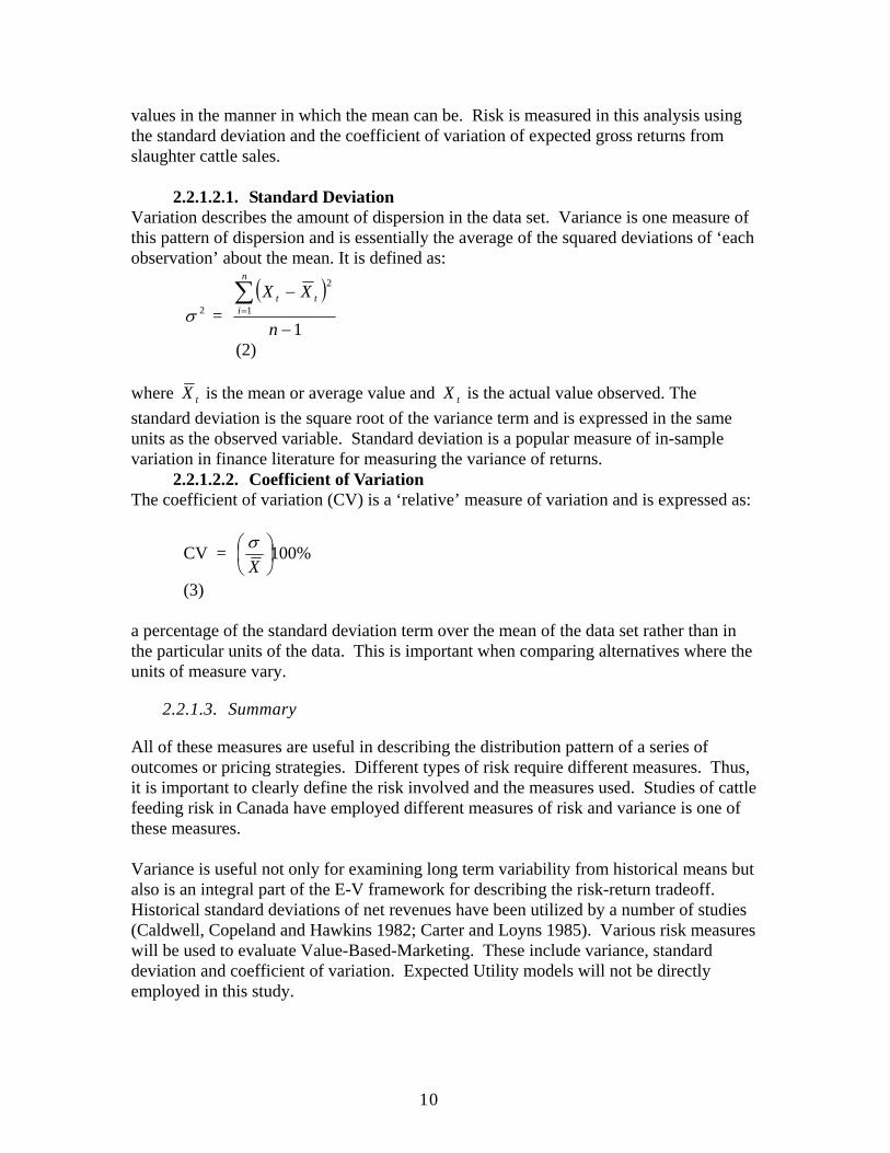
10

values in the manner in which the mean can be. Risk is measured in this analysis using the standard deviation and the coefficient of variation of expected gross returns from slaughter cattle sales.

2.2.1.2.1. Standard Deviation Variation describes the amount of dispersion in the data set. Variance is one measure of this pattern of dispersion and is essentially the average of the squared deviations of ‘each observation’ about the mean. It is defined as:

2σ = ( )

11

2

−

−∑=

n

XXn

itt

(2) where tX is the mean or average value and tX is the actual value observed. The standard deviation is the square root of the variance term and is expressed in the same units as the observed variable. Standard deviation is a popular measure of in-sample variation in finance literature for measuring the variance of returns.

2.2.1.2.2. Coefficient of Variation The coefficient of variation (CV) is a ‘relative’ measure of variation and is expressed as:

CV = %100⎟⎠⎞

⎜⎝⎛

Xσ

(3) a percentage of the standard deviation term over the mean of the data set rather than in the particular units of the data. This is important when comparing alternatives where the units of measure vary.

2.2.1.3. Summary

All of these measures are useful in describing the distribution pattern of a series of outcomes or pricing strategies. Different types of risk require different measures. Thus, it is important to clearly define the risk involved and the measures used. Studies of cattle feeding risk in Canada have employed different measures of risk and variance is one of these measures. Variance is useful not only for examining long term variability from historical means but also is an integral part of the E-V framework for describing the risk-return tradeoff. Historical standard deviations of net revenues have been utilized by a number of studies (Caldwell, Copeland and Hawkins 1982; Carter and Loyns 1985). Various risk measures will be used to evaluate Value-Based-Marketing. These include variance, standard deviation and coefficient of variation. Expected Utility models will not be directly employed in this study.

11

2.2.2. GOVERNMENT PRICE RISK MANAGEMENT INSTRUMENTS

Cattle production is a risky enterprise due in part to changing input prices and variable spot3 prices for fed cattle. In principle, production and marketing risks can be managed fairly well by diversifying portfolios, but “due to capital constraints and lifestyle considerations, many farmers and cattle feeders have a limited ability to reduce overall return risk” (Viney, 1995). It is for the purpose of stabilizing farm returns that government initiated and implemented support programs, which protect the beef industry. The National Tripartite Stabilization Program and the Crow Benefit Offset Program are two such programs. Both programs do not exist any more but their brief discussion may provide a clear picture of the evolution occurring in beef production in Alberta. The National Tripartite Stabilization Program: Prior to 1986, the U.S. and other Canadian trading partners directly subsidized their cattle producers. The federal and provincial governments responded by providing subsidies to Canadian and Alberta cattle producers to assist in stabilizing farm income. This marked the birth of the National Tripartite Stabilization Program (NTSP), implemented on January 1, 1986. Under this program, the federal and provincial governments would provide payments to producers following a period of negative net returns. NTSP was strictly for red meats, designed to stabilize prices faced by red meats producers (Bresee, 1997). “The cost of the program was shared equally by three parties; producers participating in the program, the federal and provincial governments” (Tan, 1988). NTSP provided assistance for cow-calf, backgrounding and finishing options although the finishing option was the most supported by this program in Alberta (Viney, 1995). “The finishing option of the NTSP insured a guaranteed margin on cattle and input prices. Premiums paid by producers into the program ranged from $6.60 to $8.10 per head for finishing cattle while payments from the program reached a maximum of $189.53 per head” (Munro, 1993). The NTSP provided an obvious subsidization package. This heightened trade relations between Canada and the United States whose trade policy forbids government subsidization that can be shown to harm a U.S. industry (Benson et al., 1994). Trade ties between Canada and its trading partners other than the United States were also worsening at the time. From initiation, the program was planned to continue until December 30, 1995 but given these problems, the Canadian Cattlemen’s Association was convinced that it would not be in the best interest of the beef industry to allow the program to run till the pre-planned date. As a consequence, the Canadian Cattlemen’s Association pushed for termination of the program prior to schedule. Approval for the program termination was granted for December 30, 1993, two years ahead of time . Novak et al. (1992) and Freeze et. al. (1990) reported that the NTSP significantly increased farm returns and reduced income variability. The Crow Benefit Offset Program The Crow Benefit Offset Program (CBOP) previously known as the Feeding Market Adjustment Program (FMAP) was another subsidy program of Alberta provincial government established to promote the production 3 A spot price is a price charged for a commodity in the open market.

12

and use of local feed grains (Bresee, 1997). “With feed grains not receiving the price enhancing export subsidies that other grains receive under the Western Grain Transportation Act, it was felt that Alberta producers and processors were at a competitive disadvantage” (Viney, 1995). As a result, the Alberta government enacted the CBOP and subsidized the cost of local feed grains to livestock producers. The CBOP subsidy program paid grain producers a pre-established amount per tonne of gain sold to registered users. “The program paid producers $21.00 per tonne from September 1985 to June 1987, $13.00 per tonne from July 1987 to August 1989, and $10.00 per tonne from September 1989 to March 31, 1994 (Bresee, 1997). Due to tight government budget and the move toward a competitive market, the Crow Benefit Offset Program was terminated in 1994 (Viney, 1995) at about the same with the National Tripartite Stabilization Program.

2.2.3. MARKET BASED DERIVATIVE INSTRUMENTS

Financial economics deals with many of the issues of measuring risk and pricing this component of variability. Financial models have proven to be useful instruments for valuing many of the derivative products that have emerged. These derivatives are instruments whose value are based on some underlying asset and includes futures contracts, forward contracts, and options on futures contracts. Besides providing a means for pricing and managing risk, financial models can also be used to provide comparative benchmarks. A number of standard risk tools, derivatives, exist. Futures contracts, basis, options and forward contracts are existing tools. These tools and their use are described next.

2.2.3.1. Futures Markets

Futures contracts are agreements to buy or sell a clearly defined asset for future delivery in exchange for an agreed upon price today (Hull 1995, p.1). These contracts are formally traded on a variety of exchanges; the principal one for beef cattle is the Chicago Mercantile Exchange, located in Chicago, Illinois. The primary function of futures markets is risk management. Other functions include the following: a) aiding firms in discovering forward prices, and b) providing a source of information for decision-making (Leuthold et al., 1989). The use of these markets significantly increased over the past few decades. “In the 1970s more and more raw material producers, processors and users of financial intermediaries and international trading firms use these markets to manage price, interest rate, and exchange rate risks” (Leuthold et al., 1989). Ideally cash market prices are perfectly positively correlated with futures market prices. If this condition holds, the producer’s expected profits or losses from hedging offset the cash market thus rendering the portfolio riskless. This riskless portfolio is explained below.

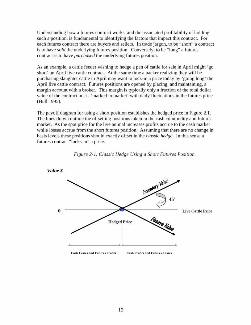
13

Understanding how a futures contract works, and the associated profitability of holding such a position, is fundamental to identifying the factors that impact this contract. For each futures contract there are buyers and sellers. In trade jargon, to be “short” a contract is to have sold the underlying futures position. Conversely, to be “long” a futures contract is to have purchased the underlying futures position. As an example, a cattle feeder wishing to hedge a pen of cattle for sale in April might ‘go short’ an April live cattle contract. At the same time a packer realizing they will be purchasing slaughter cattle in April may want to lock-in a price today by ‘going long’ the April live cattle contract. Futures positions are opened by placing, and maintaining, a margin account with a broker. This margin is typically only a fraction of the total dollar value of the contract but is ‘marked to market’ with daily fluctuations in the futures price (Hull 1995). The payoff diagram for using a short position establishes the hedged price in Figure 2.1. The lines drawn outline the offsetting positions taken in the cash commodity and futures market. As the spot price for the live animal increases profits accrue to the cash market while losses accrue from the short futures position. Assuming that there are no change in basis levels these positions should exactly offset in the classic hedge. In this sense a futures contract “locks-in” a price.

Figure 2-1. Classic Hedge Using a Short Futures Position

Value $

45º

0 Live Cattle Price Hedged Price Cash Losses and Futures Profits Cash Profits and Futures Losses

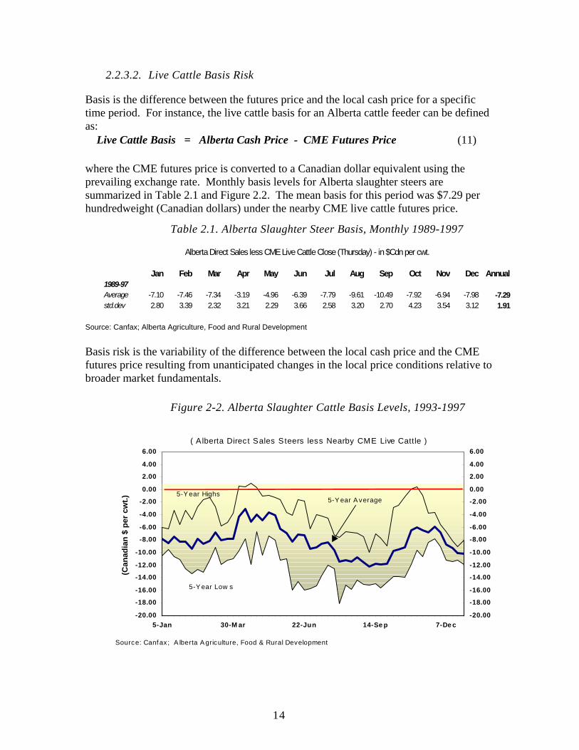
14

2.2.3.2. Live Cattle Basis Risk

Basis is the difference between the futures price and the local cash price for a specific time period. For instance, the live cattle basis for an Alberta cattle feeder can be defined as:

Live Cattle Basis = Alberta Cash Price - CME Futures Price (11) where the CME futures price is converted to a Canadian dollar equivalent using the prevailing exchange rate. Monthly basis levels for Alberta slaughter steers are summarized in Table 2.1 and Figure 2.2. The mean basis for this period was $7.29 per hundredweight (Canadian dollars) under the nearby CME live cattle futures price.

Table 2.1. Alberta Slaughter Steer Basis, Monthly 1989-1997

Alberta Direct Sales less CME Live Cattle Close (Thursday) - in $Cdn per cwt.

Jan Feb Mar Apr May Jun Jul Aug Sep Oct Nov Dec Annual1989-97Average -7.10 -7.46 -7.34 -3.19 -4.96 -6.39 -7.79 -9.61 -10.49 -7.92 -6.94 -7.98 -7.29std.dev 2.80 3.39 2.32 3.21 2.29 3.66 2.58 3.20 2.70 4.23 3.54 3.12 1.91

Source: Canfax; Alberta Agriculture, Food and Rural Development Basis risk is the variability of the difference between the local cash price and the CME futures price resulting from unanticipated changes in the local price conditions relative to broader market fundamentals.

Figure 2-2. Alberta Slaughter Cattle Basis Levels, 1993-1997

( A lberta Direct Sales Steers less Nearby CME Live Cattle )

-20.00

-18.00

-16.00

-14.00

-12.00

-10.00

-8.00

-6.00

-4.00

-2.00

0.00

2.00

4.00

6.00

5-Jan 30-M ar 22-Jun 14-Se p 7-De c

(Can

adia

n $

per c

wt.)

-20.00

-18.00

-16.00

-14.00

-12.00

-10.00

-8.00

-6.00

-4.00

-2.00

0.00

2.00

4.00

6.00

5-Y ear A verage

5-Y ear Low s

5-Y ear Highs

Source: Canfax ; A lberta A griculture, Food & Rural Development

15

Figure 2.2 highlights basis patterns and variability from 1993 through 1997, mapping the highs and lows of weekly basis over the five-year period.

2.2.3.3. Options Contracts

Options markets provide a slightly different array of pricing alternatives. Options on futures contracts also allow an individual to “lock-in” a price. The difference is that up-front premium that is paid on the option does not obligate the holder into exercising the contract. If the cash price moves in a favourable direction the upside potential is not lost. Trade in option contracts exists for numerous strike prices, above and below, the current futures price for any specific interval (contract month) of the live cattle contract. As a rule, strike prices that are closest to being at-the-money (ATM) or nearest the strike price are the most actively traded. The longer the time horizon the more likely that option trade will be somewhat less actively traded. This liquidity problem of distant option contracts creates some difficulty in establishing option premiums. An option premium can be broken down into its intrinsic value (a value that must be greater than or equal to zero) and time value as follows: Option Premium = Intrinsic Value + Time Value

= (Futures Price - Strike Price) + Time Value At expiry the time value has ‘wasted away’ to zero and any value that remains will be intrinsic value. In trade jargon, to take a “short” position is to have sold or written on an option contract on the underlying futures position. Conversely, to establish a “long” position means that you have purchased an option contract on the underlying futures position (Hull 1995, p.176). Using our cattle feeder example, a producer wishing to protect against a decline in the price of a pen of cattle for sale in April might take a ‘long position in a put option’ on April live cattle. In this case the cattle feeder has purchased the right to sell the April contract for a predetermined price. Similarly, a packer realizing they will be purchasing slaughter cattle in April may want to lock-in a price today by taking a ‘long position in a call option’ on April live cattle. This is equivalent to purchasing the right to buy the April contract at a predetermined price. Since the cattle feeder already “owns” the cattle inventory another alternative they might consider is selling the April call option. The payoff diagram for the cattle feeder long a put and short a call is illustrated in Figure 2.3. The funds received from selling the call option can be used to offset the premiums paid for buying the put option.

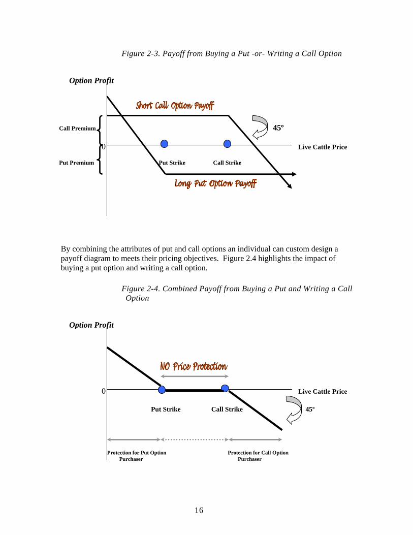
16

Figure 2-3. Payoff from Buying a Put -or- Writing a Call Option

Option Profit

Call Premium 45º

0 Live Cattle Price Put Premium Put Strike Call Strike

By combining the attributes of put and call options an individual can custom design a payoff diagram to meets their pricing objectives. Figure 2.4 highlights the impact of buying a put option and writing a call option.

Figure 2-4. Combined Payoff from Buying a Put and Writing a Call Option

Option Profit

0 Live Cattle Price Put Strike Call Strike 45º

Protection for Put Option Protection for Call Option Purchaser Purchaser

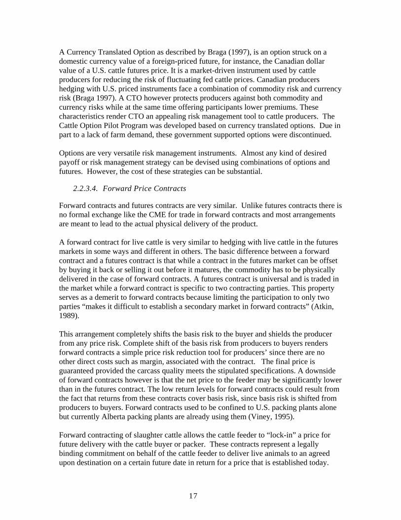
17

A Currency Translated Option as described by Braga (1997), is an option struck on a domestic currency value of a foreign-priced future, for instance, the Canadian dollar value of a U.S. cattle futures price. It is a market-driven instrument used by cattle producers for reducing the risk of fluctuating fed cattle prices. Canadian producers hedging with U.S. priced instruments face a combination of commodity risk and currency risk (Braga 1997). A CTO however protects producers against both commodity and currency risks while at the same time offering participants lower premiums. These characteristics render CTO an appealing risk management tool to cattle producers. The Cattle Option Pilot Program was developed based on currency translated options. Due in part to a lack of farm demand, these government supported options were discontinued. Options are very versatile risk management instruments. Almost any kind of desired payoff or risk management strategy can be devised using combinations of options and futures. However, the cost of these strategies can be substantial.

2.2.3.4. Forward Price Contracts

Forward contracts and futures contracts are very similar. Unlike futures contracts there is no formal exchange like the CME for trade in forward contracts and most arrangements are meant to lead to the actual physical delivery of the product. A forward contract for live cattle is very similar to hedging with live cattle in the futures markets in some ways and different in others. The basic difference between a forward contract and a futures contract is that while a contract in the futures market can be offset by buying it back or selling it out before it matures, the commodity has to be physically delivered in the case of forward contracts. A futures contract is universal and is traded in the market while a forward contract is specific to two contracting parties. This property serves as a demerit to forward contracts because limiting the participation to only two parties “makes it difficult to establish a secondary market in forward contracts” (Atkin, 1989). This arrangement completely shifts the basis risk to the buyer and shields the producer from any price risk. Complete shift of the basis risk from producers to buyers renders forward contracts a simple price risk reduction tool for producers’ since there are no other direct costs such as margin, associated with the contract. The final price is guaranteed provided the carcass quality meets the stipulated specifications. A downside of forward contracts however is that the net price to the feeder may be significantly lower than in the futures contract. The low return levels for forward contracts could result from the fact that returns from these contracts cover basis risk, since basis risk is shifted from producers to buyers. Forward contracts used to be confined to U.S. packing plants alone but currently Alberta packing plants are already using them (Viney, 1995). Forward contracting of slaughter cattle allows the cattle feeder to “lock-in” a price for future delivery with the cattle buyer or packer. These contracts represent a legally binding commitment on behalf of the cattle feeder to deliver live animals to an agreed upon destination on a certain future date in return for a price that is established today.

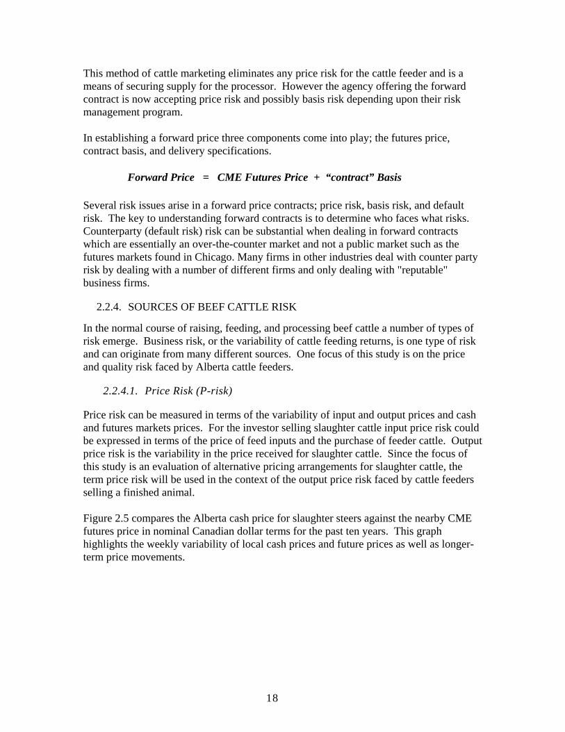
18

This method of cattle marketing eliminates any price risk for the cattle feeder and is a means of securing supply for the processor. However the agency offering the forward contract is now accepting price risk and possibly basis risk depending upon their risk management program. In establishing a forward price three components come into play; the futures price, contract basis, and delivery specifications. Forward Price = CME Futures Price + “contract” Basis Several risk issues arise in a forward price contracts; price risk, basis risk, and default risk. The key to understanding forward contracts is to determine who faces what risks. Counterparty (default risk) risk can be substantial when dealing in forward contracts which are essentially an over-the-counter market and not a public market such as the futures markets found in Chicago. Many firms in other industries deal with counter party risk by dealing with a number of different firms and only dealing with "reputable" business firms.

2.2.4. SOURCES OF BEEF CATTLE RISK

In the normal course of raising, feeding, and processing beef cattle a number of types of risk emerge. Business risk, or the variability of cattle feeding returns, is one type of risk and can originate from many different sources. One focus of this study is on the price and quality risk faced by Alberta cattle feeders.

2.2.4.1. Price Risk (P-risk)

Price risk can be measured in terms of the variability of input and output prices and cash and futures markets prices. For the investor selling slaughter cattle input price risk could be expressed in terms of the price of feed inputs and the purchase of feeder cattle. Output price risk is the variability in the price received for slaughter cattle. Since the focus of this study is an evaluation of alternative pricing arrangements for slaughter cattle, the term price risk will be used in the context of the output price risk faced by cattle feeders selling a finished animal. Figure 2.5 compares the Alberta cash price for slaughter steers against the nearby CME futures price in nominal Canadian dollar terms for the past ten years. This graph highlights the weekly variability of local cash prices and future prices as well as longer-term price movements.

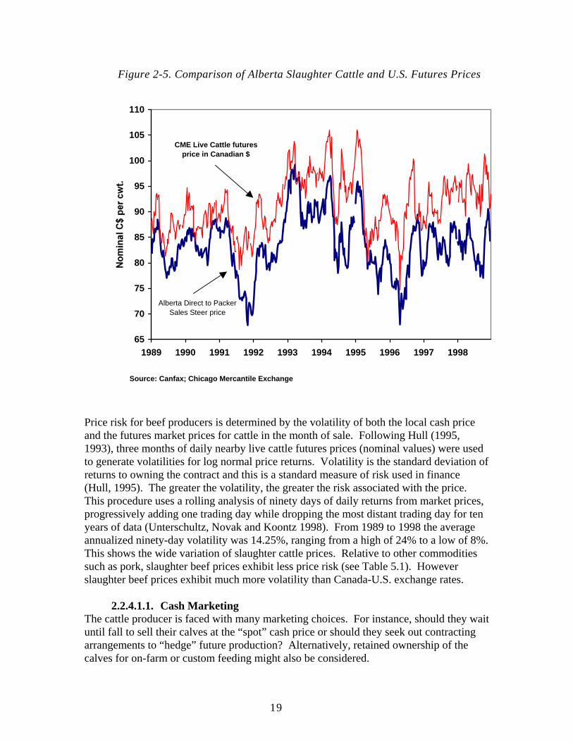
19

Figure 2-5. Comparison of Alberta Slaughter Cattle and U.S. Futures Prices

65

70

75

80

85

90

95

100

105

110

1989 1990 1991 1992 1993 1994 1995 1996 1997 1998

Source: Canfax; Chicago Mercantile Exchange

CME Live Cattle futures price in Canadian $

Alberta Direct to Packer Sales Steer price

Price risk for beef producers is determined by the volatility of both the local cash price and the futures market prices for cattle in the month of sale. Following Hull (1995, 1993), three months of daily nearby live cattle futures prices (nominal values) were used to generate volatilities for log normal price returns. Volatility is the standard deviation of returns to owning the contract and this is a standard measure of risk used in finance (Hull, 1995). The greater the volatility, the greater the risk associated with the price. This procedure uses a rolling analysis of ninety days of daily returns from market prices, progressively adding one trading day while dropping the most distant trading day for ten years of data (Unterschultz, Novak and Koontz 1998). From 1989 to 1998 the average annualized ninety-day volatility was 14.25%, ranging from a high of 24% to a low of 8%. This shows the wide variation of slaughter cattle prices. Relative to other commodities such as pork, slaughter beef prices exhibit less price risk (see Table 5.1). However slaughter beef prices exhibit much more volatility than Canada-U.S. exchange rates.

2.2.4.1.1. Cash Marketing The cattle producer is faced with many marketing choices. For instance, should they wait until fall to sell their calves at the “spot” cash price or should they seek out contracting arrangements to “hedge” future production? Alternatively, retained ownership of the calves for on-farm or custom feeding might also be considered.

20

In simple terms, the cash marketing of calves, and all cattle inventory for that matter, can be described using the following payoff diagram (Figure 2.6).

Figure 2-6. Payoff from Cash Marketing

Profit

45º

0 Live Cattle Price Break-even Price

As the cash price of calves increases, the value of the inventory also increases. Assuming a constant relationship between sales price and profitability, every dollar increase in the cash price represents additional profit. This relationship between inventory value and price can be represented by the 45° line through the break-even point. Cattle are different from a storable product such as canola. Figure 2.6 shows the value of the cattle when they are ready for market and not necessarily the value of the cattle "today". The feeding program is required to change the cattle from their current form into the form demanded by the market.

2.2.4.1.2. Futures and Forward Contracts Research in Alberta has shown that while simple routine hedging of feeder cattle using a Chicago Mercantile Exchange (CME) live cattle contract can significantly reduce risk (Unterschultz 1991), production contracting strategies which eliminate basis risk (Novak and Viney 1995) provide the best returns when evaluating a risk-return tradeoff scenario. In both cases, cattle feeders accept lower profits (the cost of the premium) in return for a hedge against financial uncertainty. These studies both suggest that the futures market can be an effective means to reducing the overall risk, but at the cost of lowering a producer’s average returns.

21

Other studies that analyze hedging as a risk management tool have reached conflicting conclusions. Carter and Loyns (1985) in their study concluded that hedging with live cattle in futures markets often reduce returns while increasing price risk for cattle. Viney (1995) commented that the authors’ results were attributed to basis variability over their study period from 1972 to 1981. Conversely, Unterschultz (1991) and others argue that hedging generally reduces risk. But he also commented that a simple routine hedge significantly reduces risk while decreasing returns only slightly. For the case of Alberta, the basis variability is high thus implying that futures markets may not be a very effective risk management instrument for Alberta cattle producers (Viney, 1995).

2.2.4.2. Exchange Rate Risk

At present there is no futures market in Canada for slaughter cattle. As a result Alberta cattle feeders must use commodity markets in the U.S. to manage price risk. This exposes producers to variability in cattle price movements between the two national markets and changes in exchange rate levels. Some studies have shown basis risk and exchange rate risk to be a significant deterrent to hedging Canadian cattle (Caldwell, Copeland and Hawkins 1982; Carter and Loyns 1985). However, a more recent analysis by Novak and Unterschultz (1991) and Unterschultz (1996) concluded that exchange rate variability contributed only a small part to the total cattle price risk, and U.S. futures contracts could be used to manage this risk. In Canada, the Cattle Options Pilot Program (COPP) also tried to bridge this market gap by providing an over-the-counter (OTC) instrument linked to the CME live cattle futures price. The COPP option is essentially a put option written on the Canadian dollar value of a CME live cattle futures contract (Braga 1997). This program began in May 1995 but was phased out in June 1998. Likely reasons for the demise of this program were the small size of the contract, the inability to arbitrage between markets if the product was perceived to be mispriced, and the general reluctance by farm managers to pay the premium for the options.4

2.2.4.3. Yield/Grade Risk (Q-risk)

The conversion of live cattle into meat introduces two more components of variability into the equation; yield and grade risk. Yield risk reflects the conversion from pounds of live animal into pounds of beef in the “carcass equivalent”. Visual approximations are the primary means for assessing the ex ante carcass yield on a live animal. After the kill floor the dressed animal moves into processing phase where the carcass is broken down into meat cuts and various by-products. A key determinant of the end value of the various meat cuts is the quality grade of the carcass. Visual measures are the predominant means of determining the carcass grade on a live animal. Pricing Grids or

4 These comments are based on the author's observations of the industry and do not reflect any direct research on the topic.

22

Value-Based-Marketing (VBM) is trying in part to address some of these yield and grade risk factors. VBM is discussed in detail in later sections

2.2.5. CONTRACTS AS ALTERNATIVE RISK MANAGEMENT TOOLS AND BASIS FOR VERTICAL COORDINATION

With termination of the two government support programs (in 1994), cattle producers were compelled to seek alternative manage risk tools. This part examines contractual agreements as a basis of vertical coordination and as the alternative risk management tool used by producers following termination of government support programs. Contracts are essentially the basis for vertical coordination if ownership remains separate. They are pricing tools used to facilitate the sale of feeder cattle. Contracts establish agreements to sell a specific number of cattle at a specific time. A contract also includes the price to be paid or how the price will be determined, the specifications feeder cattle must meet on delivery, and adjustments that will occur if specifications are not met. It is within this package of specifications that a buyer can direct the production of cattle with attributes desirable by consumers. Although these agreements usually do not spell out carcass quality characteristics (since such characteristics can only be precisely known after slaughter), contracts certainly lead to the production of beef desired by consumers and in the process reclaims lost market share. In addition, vertically coordinating with feedlots and selling cattle directly to them reduces marketing risks resulting from cattle stress and their exposure to diseases. The presence of price risk or quality risk impacts a cattle feeder either directly through a loss in revenue or wealth or indirectly through changes in their decision-making process. In the short term, risk creates liquidity concerns with uncertainty in cash flows, changes in asset values, or the availability of credit. In the longer term, risk can also impact the sources and uses of these cash flows and the investment alternatives.

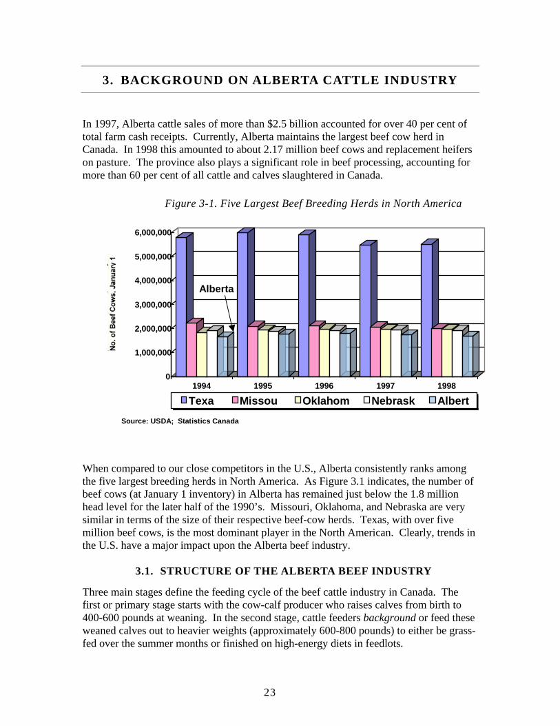
23

3. BACKGROUND ON ALBERTA CATTLE INDUSTRY

In 1997, Alberta cattle sales of more than $2.5 billion accounted for over 40 per cent of total farm cash receipts. Currently, Alberta maintains the largest beef cow herd in Canada. In 1998 this amounted to about 2.17 million beef cows and replacement heifers on pasture. The province also plays a significant role in beef processing, accounting for more than 60 per cent of all cattle and calves slaughtered in Canada.

Figure 3-1. Five Largest Beef Breeding Herds in North America

0

1,000,000

2,000,000

3,000,000

4,000,000

5,000,000

6,000,000

1994 1995 1996 1997 1998

Texa Missou Oklahom Nebrask Albert

Alberta

Source: USDA; Statistics Canada

When compared to our close competitors in the U.S., Alberta consistently ranks among the five largest breeding herds in North America. As Figure 3.1 indicates, the number of beef cows (at January 1 inventory) in Alberta has remained just below the 1.8 million head level for the later half of the 1990’s. Missouri, Oklahoma, and Nebraska are very similar in terms of the size of their respective beef-cow herds. Texas, with over five million beef cows, is the most dominant player in the North American. Clearly, trends in the U.S. have a major impact upon the Alberta beef industry.

3.1. STRUCTURE OF THE ALBERTA BEEF INDUSTRY

Three main stages define the feeding cycle of the beef cattle industry in Canada. The first or primary stage starts with the cow-calf producer who raises calves from birth to 400-600 pounds at weaning. In the second stage, cattle feeders background or feed these weaned calves out to heavier weights (approximately 600-800 pounds) to either be grass-fed over the summer months or finished on high-energy diets in feedlots.

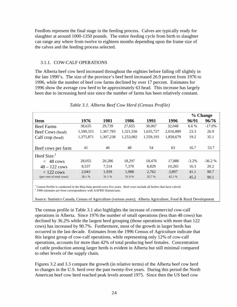
24

Feedlots represent the final stage in the feeding process. Calves are typically ready for slaughter at around 1000-1350 pounds. The entire feeding cycle from birth to slaughter can range any where from twelve to eighteen months depending upon the frame size of the calves and the feeding process selected.

3.1.1. COW-CALF OPERATIONS

The Alberta beef cow herd increased throughout the eighties before falling off slightly in the late 1990’s. The size of the province’s beef herd increased 26.9 percent from 1976 to 1996, while the number of beef cow farms declined by over 17 percent. Estimates for 1996 show the average cow herd to be approximately 63 head. This increase has largely been due to increasing herd size since the number of farms has been relatively constant.

Table 3.1. Alberta Beef Cow Herd (Census Profile)

% Change Item 1976 1981 1986 1991 1996 96/91 96/76 Beef Farms 38,635 29,739 27,655 30,067 32,048 6.6 % -17.0% Beef Cows (head) 1,590,315 1,367,783 1,321,556 1,635,727 2,016,889 23.3 26.9 Calf crop (head) 1,375,871 1,307,238 1,253,082 1,559,193 1,858,679 19.2 35.1 Beef cows per farm 41 46 48 54 63 16.7 53.7

Herd Size:1 < 48 cows 28,055 20,286 18,297 18,476 17,886 -3.2% -36.2 %

48 – 122 cows 8,537 7,514 7,370 8,829 10,265 16.3 20.2 > 122 cows 2,043 1,939 1,988 2,762 3,897 41.1 90.7

(per cent of total cows) 28.1 % 31.1 % 31.9 % 35.7 % 42.1 % 45.2 90.1

* Census Profile is conducted in the May/June period every five years. Beef cows include all heifers that have calved. 1 1996 estimates are from correspondence with AAFRD Statisticians. Source: Statistics Canada, Census of Agriculture (various years); Alberta Agriculture, Food & Rural Development The census profile in Table 3.1 also highlights the increase of commercial cow-calf operations in Alberta. Since 1976 the number of small operations (less than 48 cows) has declined by 36.2% while the largest herd grouping (those operations with more than 122 cows) has increased by 90.7%. Furthermore, most of the growth in larger herds has occurred in the last decade. Estimates from the 1996 Census of Agriculture indicate that this largest group of cow-calf operations, while representing only 12% of cow-calf operations, accounts for more than 42% of total producing beef females. Concentration of cattle production among larger herds is evident in Alberta but still minimal compared to other levels of the supply chain. Figures 3.2 and 3.3 compare the growth (in relative terms) of the Alberta beef cow herd to changes in the U.S. herd over the past twenty-five years. During this period the North American beef cow herd reached peak levels around 1975. Since then the US beef cow

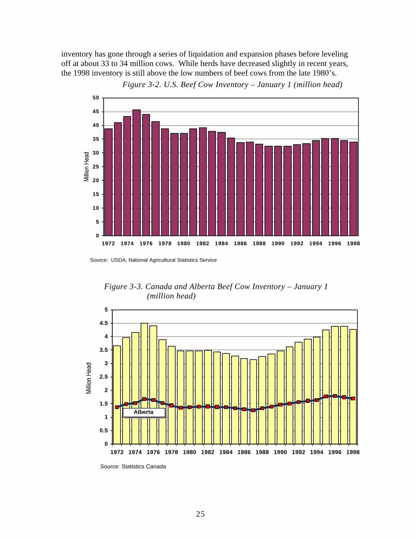
25

inventory has gone through a series of liquidation and expansion phases before leveling off at about 33 to 34 million cows. While herds have decreased slightly in recent years, the 1998 inventory is still above the low numbers of beef cows from the late 1980’s.

Figure 3-2. U.S. Beef Cow Inventory – January 1 (million head)

0

5

10

15

20

25

30

35

40

45

50

1972 1974 1976 1978 1980 1982 1984 1986 1988 1990 1992 1994 1996 1998

Source: USDA, National Agricultural Statistics Service

Figure 3-3. Canada and Alberta Beef Cow Inventory – January 1 (million head)

0

0.5

1

1.5

2

2.5

3

3.5

4

4.5

5

1972 1974 1976 1978 1980 1982 1984 1986 1988 1990 1992 1994 1996 1998

Source: Statistics Canada

Alberta

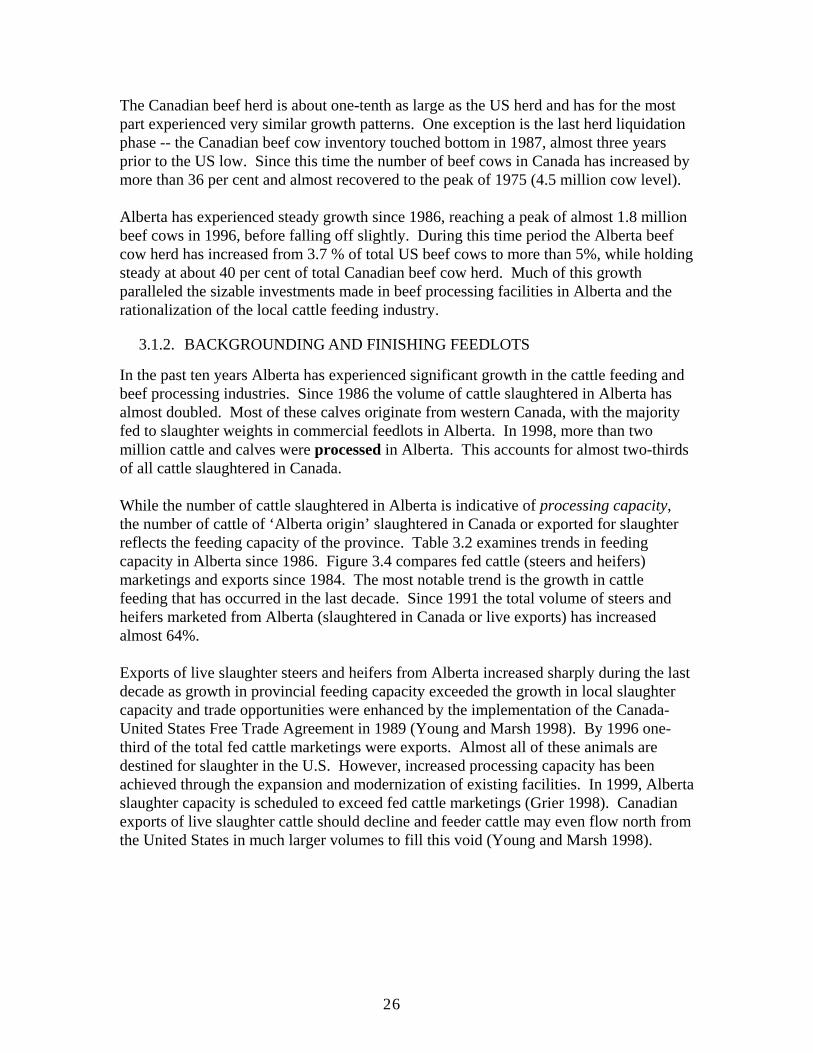
26

The Canadian beef herd is about one-tenth as large as the US herd and has for the most part experienced very similar growth patterns. One exception is the last herd liquidation phase -- the Canadian beef cow inventory touched bottom in 1987, almost three years prior to the US low. Since this time the number of beef cows in Canada has increased by more than 36 per cent and almost recovered to the peak of 1975 (4.5 million cow level). Alberta has experienced steady growth since 1986, reaching a peak of almost 1.8 million beef cows in 1996, before falling off slightly. During this time period the Alberta beef cow herd has increased from 3.7 % of total US beef cows to more than 5%, while holding steady at about 40 per cent of total Canadian beef cow herd. Much of this growth paralleled the sizable investments made in beef processing facilities in Alberta and the rationalization of the local cattle feeding industry.

3.1.2. BACKGROUNDING AND FINISHING FEEDLOTS

In the past ten years Alberta has experienced significant growth in the cattle feeding and beef processing industries. Since 1986 the volume of cattle slaughtered in Alberta has almost doubled. Most of these calves originate from western Canada, with the majority fed to slaughter weights in commercial feedlots in Alberta. In 1998, more than two million cattle and calves were processed in Alberta. This accounts for almost two-thirds of all cattle slaughtered in Canada. While the number of cattle slaughtered in Alberta is indicative of processing capacity, the number of cattle of ‘Alberta origin’ slaughtered in Canada or exported for slaughter reflects the feeding capacity of the province. Table 3.2 examines trends in feeding capacity in Alberta since 1986. Figure 3.4 compares fed cattle (steers and heifers) marketings and exports since 1984. The most notable trend is the growth in cattle feeding that has occurred in the last decade. Since 1991 the total volume of steers and heifers marketed from Alberta (slaughtered in Canada or live exports) has increased almost 64%. Exports of live slaughter steers and heifers from Alberta increased sharply during the last decade as growth in provincial feeding capacity exceeded the growth in local slaughter capacity and trade opportunities were enhanced by the implementation of the Canada-United States Free Trade Agreement in 1989 (Young and Marsh 1998). By 1996 one-third of the total fed cattle marketings were exports. Almost all of these animals are destined for slaughter in the U.S. However, increased processing capacity has been achieved through the expansion and modernization of existing facilities. In 1999, Alberta slaughter capacity is scheduled to exceed fed cattle marketings (Grier 1998). Canadian exports of live slaughter cattle should decline and feeder cattle may even flow north from the United States in much larger volumes to fill this void (Young and Marsh 1998).

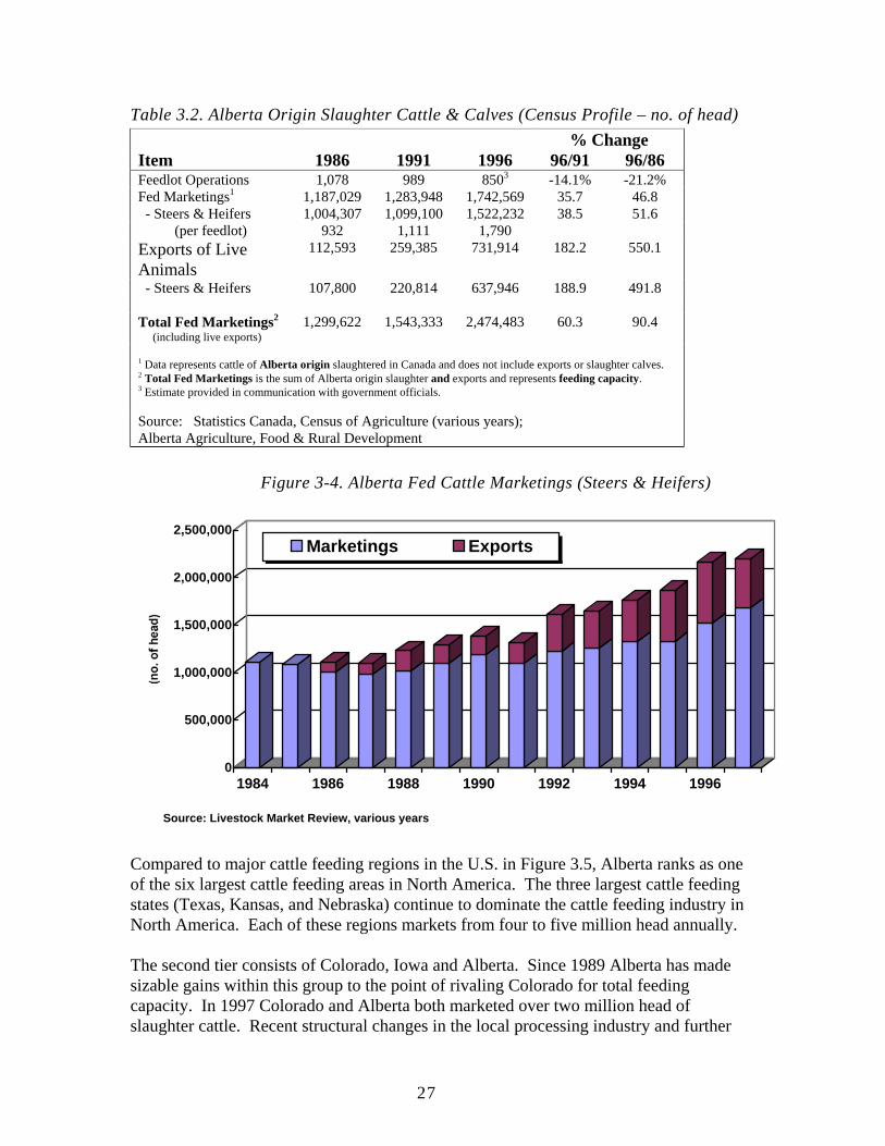
27

Table 3.2. Alberta Origin Slaughter Cattle & Calves (Census Profile – no. of head) % Change Item 1986 1991 1996 96/91 96/86 Feedlot Operations 1,078 989 8503 -14.1% -21.2% Fed Marketings1 1,187,029 1,283,948 1,742,569 35.7 46.8 - Steers & Heifers 1,004,307 1,099,100 1,522,232 38.5 51.6

(per feedlot) 932 1,111 1,790 Exports of Live Animals

112,593 259,385 731,914 182.2 550.1

- Steers & Heifers 107,800 220,814 637,946 188.9 491.8 Total Fed Marketings2 (including live exports)

1,299,622 1,543,333 2,474,483 60.3 90.4

1 Data represents cattle of Alberta origin slaughtered in Canada and does not include exports or slaughter calves. 2 Total Fed Marketings is the sum of Alberta origin slaughter and exports and represents feeding capacity. 3 Estimate provided in communication with government officials. Source: Statistics Canada, Census of Agriculture (various years); Alberta Agriculture, Food & Rural Development

Figure 3-4. Alberta Fed Cattle Marketings (Steers & Heifers)

Compared to major cattle feeding regions in the U.S. in Figure 3.5, Alberta ranks as one of the six largest cattle feeding areas in North America. The three largest cattle feeding states (Texas, Kansas, and Nebraska) continue to dominate the cattle feeding industry in North America. Each of these regions markets from four to five million head annually. The second tier consists of Colorado, Iowa and Alberta. Since 1989 Alberta has made sizable gains within this group to the point of rivaling Colorado for total feeding capacity. In 1997 Colorado and Alberta both marketed over two million head of slaughter cattle. Recent structural changes in the local processing industry and further

0

500,000

1,000,000

1,500,000

2,000,000

2,500,000

1984 1986 1988 1990 1992 1994 1996

Marketings Exports

Source: Livestock Market Review, various years

28

growth of the Alberta cattle feeding industry could increase the relative importance of Alberta within this group even more.

Figure 3-5 Major Feeding Areas in North America

0

1,000,000

2,000,000

3,000,000

4,000,000

5,000,000

6,000,000

1989* 1993 1994 1995 1996 1997Texas Kansas Nebraska Colorado Iowa Alberta

Source: USDA, NASS; Agriculture Canada,Livestock Market Review (various years)

3.1.3. PROCESSING INDUSTRY

The major players in the Canadian beef processing industry are Excel (Cargill Foods) in High River (Alberta), IBP (Lakeside Packers) in Brooks (Alberta), Better Beef Limited in Guelph (Ontario), and X-L Foods Ltd in Calgary (Alberta). Together these four packers slaughtered about 70% of all federally inspected cattle in Canada in 1997 (Agriculture and Agri-food Canada 1997; Grier 1998). This compares with a four-firm concentration ratio of only 43% in 1991 (CITT 1993). As Excel and IBP, the two largest firms, strive for even further scale economies the industry will likely become even more concentrated. The degree of packer concentration in Canada closely follows the pattern emerging in the United States (Young and Marsh 1998). In 1997, the four largest packers in the U.S. accounted for over 68% of total cattle slaughter and 80% of all steers and heifers. Such high levels of concentration have precipitated numerous studies into the extent of market power and captive supplies in the North American beef industry (Koontz and Purcell 1997).

3.2. CONSUMERS: DOMESTIC AND EXPORT MARKETS

Beef cattle are a valuable resource to the Canadian economy, feeding a growing population and providing export revenue. Canadians consume, on average, almost one million tonnes of beef and beef products per year or the equivalent of about 31.6

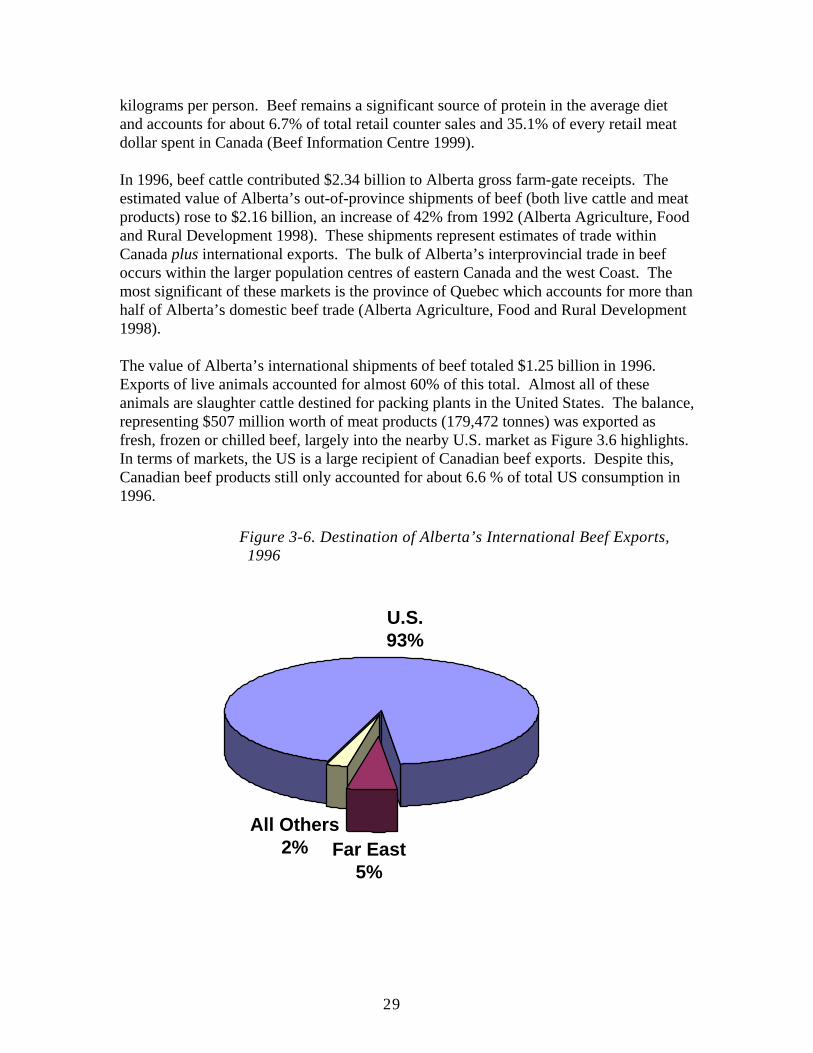
29

kilograms per person. Beef remains a significant source of protein in the average diet and accounts for about 6.7% of total retail counter sales and 35.1% of every retail meat dollar spent in Canada (Beef Information Centre 1999). In 1996, beef cattle contributed $2.34 billion to Alberta gross farm-gate receipts. The estimated value of Alberta’s out-of-province shipments of beef (both live cattle and meat products) rose to $2.16 billion, an increase of 42% from 1992 (Alberta Agriculture, Food and Rural Development 1998). These shipments represent estimates of trade within Canada plus international exports. The bulk of Alberta’s interprovincial trade in beef occurs within the larger population centres of eastern Canada and the west Coast. The most significant of these markets is the province of Quebec which accounts for more than half of Alberta’s domestic beef trade (Alberta Agriculture, Food and Rural Development 1998). The value of Alberta’s international shipments of beef totaled $1.25 billion in 1996. Exports of live animals accounted for almost 60% of this total. Almost all of these animals are slaughter cattle destined for packing plants in the United States. The balance, representing $507 million worth of meat products (179,472 tonnes) was exported as fresh, frozen or chilled beef, largely into the nearby U.S. market as Figure 3.6 highlights. In terms of markets, the US is a large recipient of Canadian beef exports. Despite this, Canadian beef products still only accounted for about 6.6 % of total US consumption in 1996.

Figure 3-6. Destination of Alberta’s International Beef Exports, 1996

U.S.93%

Far East5%

All Others2%

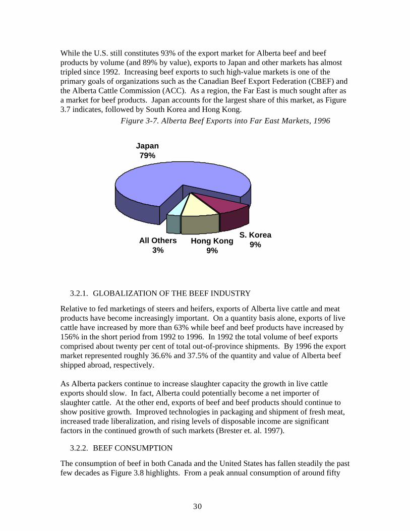
30

While the U.S. still constitutes 93% of the export market for Alberta beef and beef products by volume (and 89% by value), exports to Japan and other markets has almost tripled since 1992. Increasing beef exports to such high-value markets is one of the primary goals of organizations such as the Canadian Beef Export Federation (CBEF) and the Alberta Cattle Commission (ACC). As a region, the Far East is much sought after as a market for beef products. Japan accounts for the largest share of this market, as Figure 3.7 indicates, followed by South Korea and Hong Kong.

Figure 3-7. Alberta Beef Exports into Far East Markets, 1996

Japan79%

S. Korea9%Hong Kong

9%All Others

3%

3.2.1. GLOBALIZATION OF THE BEEF INDUSTRY

Relative to fed marketings of steers and heifers, exports of Alberta live cattle and meat products have become increasingly important. On a quantity basis alone, exports of live cattle have increased by more than 63% while beef and beef products have increased by 156% in the short period from 1992 to 1996. In 1992 the total volume of beef exports comprised about twenty per cent of total out-of-province shipments. By 1996 the export market represented roughly 36.6% and 37.5% of the quantity and value of Alberta beef shipped abroad, respectively. As Alberta packers continue to increase slaughter capacity the growth in live cattle exports should slow. In fact, Alberta could potentially become a net importer of slaughter cattle. At the other end, exports of beef and beef products should continue to show positive growth. Improved technologies in packaging and shipment of fresh meat, increased trade liberalization, and rising levels of disposable income are significant factors in the continued growth of such markets (Brester et. al. 1997).

3.2.2. BEEF CONSUMPTION

The consumption of beef in both Canada and the United States has fallen steadily the past few decades as Figure 3.8 highlights. From a peak annual consumption of around fifty

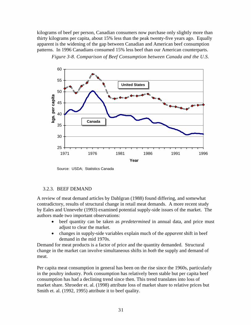
31

kilograms of beef per person, Canadian consumers now purchase only slightly more than thirty kilograms per capita, about 15% less than the peak twenty-five years ago. Equally apparent is the widening of the gap between Canadian and American beef consumption patterns. In 1996 Canadians consumed 15% less beef than our American counterparts.

Figure 3-8. Comparison of Beef Consumption between Canada and the U.S.

25

30

35

40

45

50

55

60

1971 1976 1981 1986 1991 1996

Year

Source: USDA; Statistics Canada

Canada

United States

3.2.3. BEEF DEMAND

A review of meat demand articles by Dahlgran (1988) found differing, and somewhat contradictory, results of structural change in retail meat demands. A more recent study by Eales and Unnevehr (1993) examined potential supply-side issues of the market. The authors made two important observations:

• beef quantity can be taken as predetermined in annual data, and price must adjust to clear the market.

• changes in supply-side variables explain much of the apparent shift in beef demand in the mid 1970s.

Demand for meat products is a factor of price and the quantity demanded. Structural change in the market can involve simultaneous shifts in both the supply and demand of meat. Per capita meat consumption in general has been on the rise since the 1960s, particularly in the poultry industry. Pork consumption has relatively been stable but per capita beef consumption has had a declining trend since then. This trend translates into loss of market share. Shroeder et. al. (1998) attribute loss of market share to relative prices but Smith et. al. (1992, 1995) attribute it to beef quality.

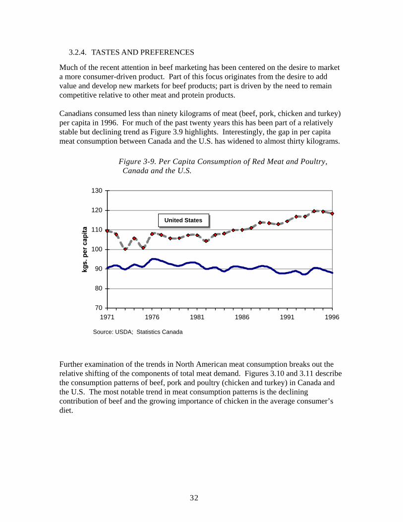
32

3.2.4. TASTES AND PREFERENCES

Much of the recent attention in beef marketing has been centered on the desire to market a more consumer-driven product. Part of this focus originates from the desire to add value and develop new markets for beef products; part is driven by the need to remain competitive relative to other meat and protein products. Canadians consumed less than ninety kilograms of meat (beef, pork, chicken and turkey) per capita in 1996. For much of the past twenty years this has been part of a relatively stable but declining trend as Figure 3.9 highlights. Interestingly, the gap in per capita meat consumption between Canada and the U.S. has widened to almost thirty kilograms.

Figure 3-9. Per Capita Consumption of Red Meat and Poultry, Canada and the U.S.

70

80

90

100

110

120

130

1971 1976 1981 1986 1991 1996

United States

Source: USDA; Statistics Canada

Further examination of the trends in North American meat consumption breaks out the relative shifting of the components of total meat demand. Figures 3.10 and 3.11 describe the consumption patterns of beef, pork and poultry (chicken and turkey) in Canada and the U.S. The most notable trend in meat consumption patterns is the declining contribution of beef and the growing importance of chicken in the average consumer’s diet.

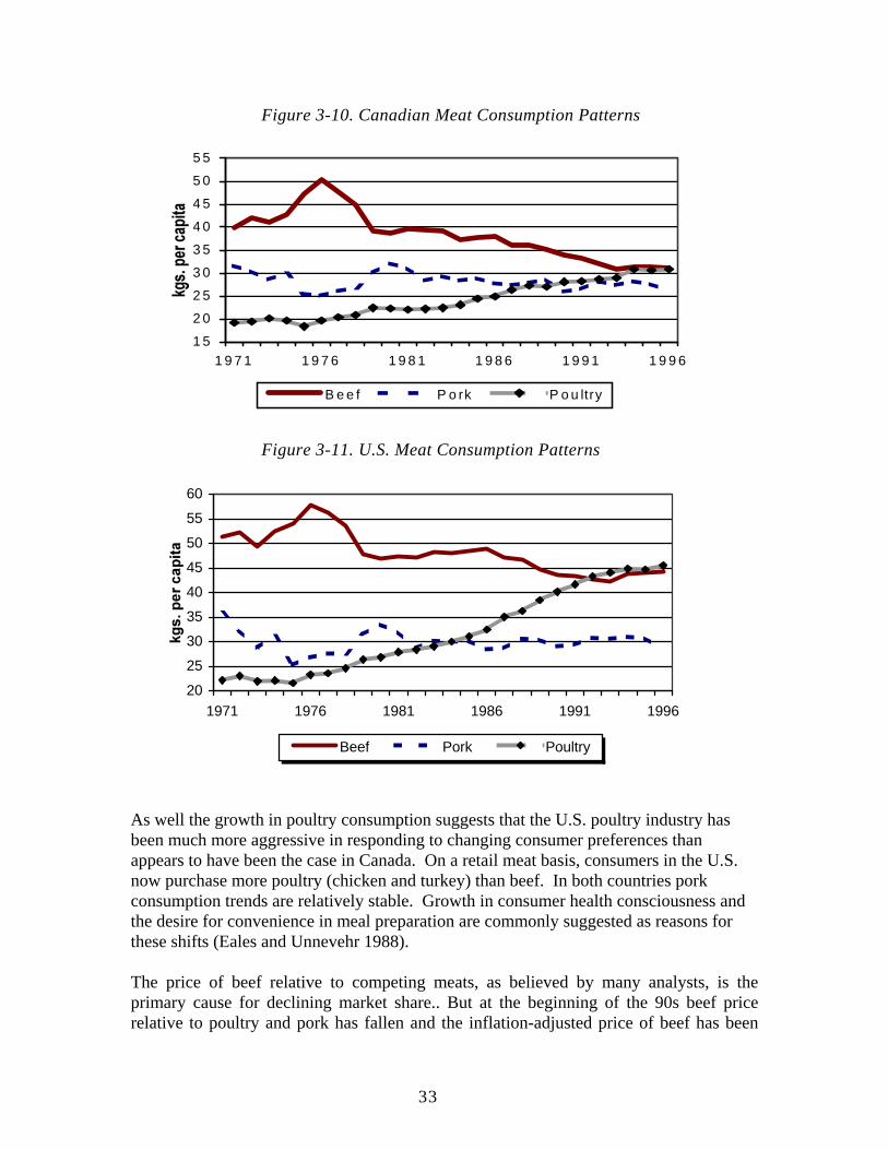
33

Figure 3-10. Canadian Meat Consumption Patterns

1 52 02 53 03 5

4 04 5

5 05 5

1 9 7 1 1 9 7 6 1 9 8 1 1 9 8 6 1 9 9 1 1 9 9 6

B e e f P o rk P o u ltry

Figure 3-11. U.S. Meat Consumption Patterns

20

253035404550

5560

1971 1976 1981 1986 1991 1996

Beef Pork Poultry

As well the growth in poultry consumption suggests that the U.S. poultry industry has been much more aggressive in responding to changing consumer preferences than appears to have been the case in Canada. On a retail meat basis, consumers in the U.S. now purchase more poultry (chicken and turkey) than beef. In both countries pork consumption trends are relatively stable. Growth in consumer health consciousness and the desire for convenience in meal preparation are commonly suggested as reasons for these shifts (Eales and Unnevehr 1988). The price of beef relative to competing meats, as believed by many analysts, is the primary cause for declining market share.. But at the beginning of the 90s beef price relative to poultry and pork has fallen and the inflation-adjusted price of beef has been

34

declining for several years now (Lamb and Beshear, 1998). Despite this shift in relative prices, the beef industry has not reclaimed its lost market share thus calling into question price factors as being the root cause for the industry's loss of market share. Nonprice factors such as lack of consistency in beef quality, changes in lifestyle and health concerns affect the demand for beef. Concerning health, consumers are concerned about the fat and cholesterol levels in meat. The pork industry has addressed these concerns by reducing the fat content in pork, but to the contrary, the current grading system of the beef industry used in evaluating carcass actually rewards beef for marbling since fat is generally believed to enhance tenderness and taste (Lamb and Beshear, 1998). To health-conscious consumers however, this may be a demerit. Many market analysts have reasoned that while consumer behavior and taste is changing, the beef industry has not kept pace with this change by developing products that meet the changing demand of consumers. For instance, there may be a lack of consistent quality in beef (Lamb and Beshear, 1998). Also change in lifestyle certainly affects the demand for beef. In particular the entry of women into the workforce in larger numbers resulted in increasing demand for conveniently packed and fast cooking food products. In 1977, 46.7% of women participated in the labor force (Statistics Canada, 1998). Statistics Canada indicates that over the past two decades the rate has increased to 57.4%. With the growing number of women going into the labor force most households have sharply cut down on the time spent in preparing food. Unlike the poultry industry that has responded by supplying convenient food products, the beef industry has lagged behind in supplying similar food products. The structures of the pork and poultry industries lend themselves suitable for coordinated production. As much as 93% of the U.S. share of broilers and 32% of its pork share are produced under contractual agreements (Barkema, Drabenstott and Welch, 1991). Vertical coordination has proved successful in the U.S. pork and poultry industries.

3.3. CURRENT MARKETING ARRANGEMENTS

To estimate the price aspects of vertical coordination in the Alberta cattle feeding sector, the prices received throughout different stages of the marketing process must be evaluated. Price is determined by the interaction of the forces of supply and demand. Beef demand reflects the quantity of beef products that consumers are willing to purchase. The supply of beef is in turn measured by the quantity and quality of slaughter animals entering the processing phase of beef production. How well price reflects the individual characteristics of these animals is important in determining end-value and providing economic incentives to primary producers in a coordinated system. Price is an important signal for encouraging the production of beef products most demanded by consumers. In general the pricing element of these markets provides two functions (Buse and Bromley 1975, pp.7-12);

• allocates resources among alternative uses, and • provides the means to coordinate the cattle production and beef marketing

stages consistent with the demand of consumers

35

Studies of pricing efficiency in beef cattle marketing have examined both the feeder and slaughter cattle markets. Characteristics such as sex, weight, breed, pen size, seasonality, and dressed weight prices have all been shown to impact the price of feeder cattle in the U.S. (Ward 1987). Slaughter cattle pricing has tended to reflect quality concerns and the wholesale value of beef products.

3.3.1. MARKETING METHODS IN THE ALBERTA BEEF INDUSTRY

Several distinct levels of production in the Alberta beef industry were identified. Different profit margins, resource requirements, and degrees of market power characterize each of these vertical levels of the production chain, from the primary producer to the food retailer.

3.3.1.1. Cow-Calf Feeder

The majority of cow-calf operators wean calves in the fall once they reach about six months of age. This means that large numbers of feeder calves typically hit the market between September and November depending on the availability of grazing and the onset of the winter feeding period. Cow-calf producers are for the most part price-takers. Weaned calves are typically sorted for sale into three basic market settings: public auction, private treaty or direct sales between individuals, and sale via electronic means of communication (Figure 3.12). The traditional marketing process of the public auction relies on the ‘live’ interaction between buyers and sellers. Cattle are priced on the spot as they move through an auction ring. These public auction sales are generally centralized local points and terminal yards and remain the most dominant form of pricing feeder cattle (Tronstad 1994). Private treaty or direct sales occur when individual cow-calf operators and cattle feeders individually negotiate the terms and conditions of the sale. In this instance price is determined outside of the normal bid process. Developments in communication technology have greatly expanded the spatial component of livestock markets. Satellite video sales and computer trading try to replicate the instantaneous interaction of buyers and sellers by electronic modes of communication. Standardized information regarding the sales terms and cattle description (breed type, sex, and weight) as well as location and identity of the seller become the proxy for the “real-time” animal description. This information is a vital component of electronic marketing and necessary for pricing efficiency. Furthermore, electronic marketing provides much broader coverage of potential buyers and offers the opportunity to forward contract since immediate possession of sale animals is not a precursor to transfer of title. For instance, the seller may offer to contract feed the cattle or establish a time frame for forward delivery.

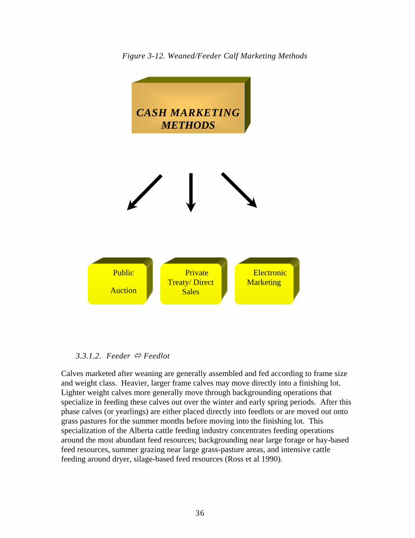
36

Figure 3-12. Weaned/Feeder Calf Marketing Methods

3.3.1.2. Feeder Feedlot

Calves marketed after weaning are generally assembled and fed according to frame size and weight class. Heavier, larger frame calves may move directly into a finishing lot. Lighter weight calves more generally move through backgrounding operations that specialize in feeding these calves out over the winter and early spring periods. After this phase calves (or yearlings) are either placed directly into feedlots or are moved out onto grass pastures for the summer months before moving into the finishing lot. This specialization of the Alberta cattle feeding industry concentrates feeding operations around the most abundant feed resources; backgrounding near large forage or hay-based feed resources, summer grazing near large grass-pasture areas, and intensive cattle feeding around dryer, silage-based feed resources (Ross et al 1990).

CASH MARKETINGMETHODS

Public

Auction

Private Treaty/ Direct

Sales

Electronic Marketing

37

Cattle entering a finishing lot may be placed directly in the feedlot by individual cattle feeders, purchased by the feedlot, or placed on feed by outside investors. The ownership of these cattle in the feedlot influences price determination at this stage. The growth of large finishing feedlots has led to significant capital investments and increased reliance on custom feeding to run these operations at full capacity. Quite often feedlots use cattle dealers or order buyers to assemble the size and type of cattle they desire.

3.3.1.3. Feedlot Processor

Generally speaking the marketing of slaughter cattle is similar in form to the model presented for feeder cattle in Figure 3.12. Data from the three largest packers in Alberta suggests that cash sales are still the predominant means of marketing slaughter cattle. More than two-thirds of slaughter cattle procured in 1998 were purchased on a cash basis, 22 % by some means of captive supply (contracted or packer-owned fed cattle) and 10 % by formula or grid arrangements (Canfax 1999). Fed cattle are marketed through one of two channels in Alberta; either direct to packer or through an auction market or some form of commission house (Dunford 1996). Differences exist however in the alternatives for pricing fed cattle since the end product can be sold on either a live animal or beef basis. The choices facing Alberta feedlot operators in pricing slaughter cattle to processors are outlined in Figure 3.13. First, animals can be sold either on a live weight or dressed weight basis. Selling animals “live” means that the processor assumes all risk for how the animals will yield and ultimately grade out. The live weight price received is essentially factored back from the wholesale price and an estimate of slaughter cattle traits (dressing percentage, cutability and grade) to determine an average price for a pen of cattle. Once animals pass through the kill floor the carcass equivalent of the live animal becomes the focal pricing point. Selling animals in the “beef” means that the cattle feeder assumes all risk for how the animals will dress out as a carcass beef and in some instances how animals will ultimately yield and grade out. At this stage the animal can be priced according to the dressed weight and an estimate of carcass merit (cutability and quality grade) to determine an average price for a pen of cattle. Alternatively, carcasses can be individually graded and priced according to quality and yield merits. This method of pricing comes closest to measuring the value added by an individual carcass.

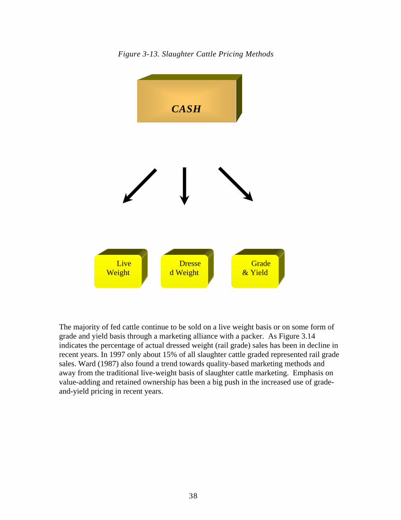
38

Figure 3-13. Slaughter Cattle Pricing Methods

The majority of fed cattle continue to be sold on a live weight basis or on some form of grade and yield basis through a marketing alliance with a packer. As Figure 3.14 indicates the percentage of actual dressed weight (rail grade) sales has been in decline in recent years. In 1997 only about 15% of all slaughter cattle graded represented rail grade sales. Ward (1987) also found a trend towards quality-based marketing methods and away from the traditional live-weight basis of slaughter cattle marketing. Emphasis on value-adding and retained ownership has been a big push in the increased use of grade-and-yield pricing in recent years.

CASH

Live Weight

Dressed Weight

Grade & Yield

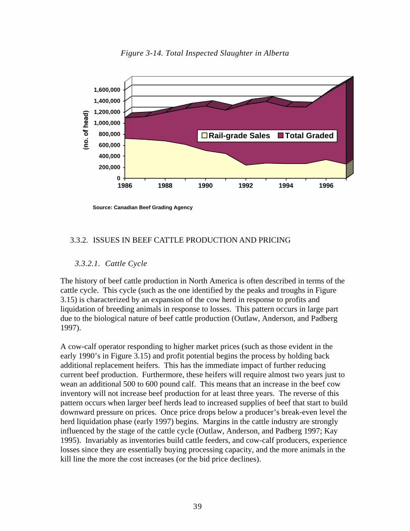
39

Figure 3-14. Total Inspected Slaughter in Alberta

0

200,000

400,000

600,000

800,000

1,000,000

1,200,000

1,400,000

1,600,000

1986 1988 1990 1992 1994 1996

Rail-grade Sales Total Graded

Source: Canadian Beef Grading Agency

3.3.2. ISSUES IN BEEF CATTLE PRODUCTION AND PRICING

3.3.2.1. Cattle Cycle

The history of beef cattle production in North America is often described in terms of the cattle cycle. This cycle (such as the one identified by the peaks and troughs in Figure 3.15) is characterized by an expansion of the cow herd in response to profits and liquidation of breeding animals in response to losses. This pattern occurs in large part due to the biological nature of beef cattle production (Outlaw, Anderson, and Padberg 1997). A cow-calf operator responding to higher market prices (such as those evident in the early 1990’s in Figure 3.15) and profit potential begins the process by holding back additional replacement heifers. This has the immediate impact of further reducing current beef production. Furthermore, these heifers will require almost two years just to wean an additional 500 to 600 pound calf. This means that an increase in the beef cow inventory will not increase beef production for at least three years. The reverse of this pattern occurs when larger beef herds lead to increased supplies of beef that start to build downward pressure on prices. Once price drops below a producer’s break-even level the herd liquidation phase (early 1997) begins. Margins in the cattle industry are strongly influenced by the stage of the cattle cycle (Outlaw, Anderson, and Padberg 1997; Kay 1995). Invariably as inventories build cattle feeders, and cow-calf producers, experience losses since they are essentially buying processing capacity, and the more animals in the kill line the more the cost increases (or the bid price declines).

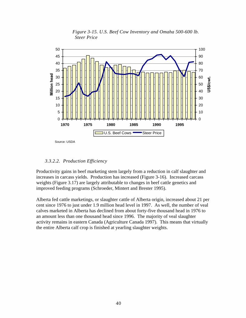
40

Figure 3-15. U.S. Beef Cow Inventory and Omaha 500-600 lb. Steer Price

0

5

10

15

20

25

30

35

40

45

50

1970 1975 1980 1985 1990 19950

10

20

30

40

50

60

70

80

90

100

U.S. Beef Cows Steer Price

Source: USDA

3.3.2.2. Production Efficiency

Productivity gains in beef marketing stem largely from a reduction in calf slaughter and increases in carcass yields. Production has increased (Figure 3-16). Increased carcass weights (Figure 3.17) are largely attributable to changes in beef cattle genetics and improved feeding programs (Schroeder, Mintert and Brester 1995). Alberta fed cattle marketings, or slaughter cattle of Alberta origin, increased about 21 per cent since 1976 to just under 1.9 million head level in 1997. As well, the number of veal calves marketed in Alberta has declined from about forty-five thousand head in 1976 to an amount less than one thousand head since 1996. The majority of veal slaughter activity remains in eastern Canada (Agriculture Canada 1997). This means that virtually the entire Alberta calf crop is finished at yearling slaughter weights.

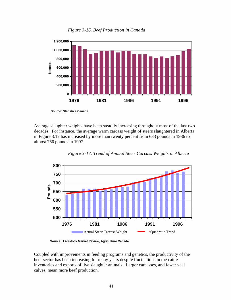
41

Figure 3-16. Beef Production in Canada

0

200,000

400,000

600,000

800,000

1,000,000

1,200,000

1976 1981 1986 1991 1996

Source: Statistics Canada

Average slaughter weights have been steadily increasing throughout most of the last two decades. For instance, the average warm carcass weight of steers slaughtered in Alberta in Figure 3.17 has increased by more than twenty percent from 633 pounds in 1986 to almost 766 pounds in 1997.

Figure 3-17. Trend of Annual Steer Carcass Weights in Alberta

500

550

600

650

700

750

800

1976 1981 1986 1991 1996Actual Steer Carcass Weight Quadratic Trend

Source: Livestock Market Review, Agriculture Canada

Coupled with improvements in feeding programs and genetics, the productivity of the beef sector has been increasing for many years despite fluctuations in the cattle inventories and exports of live slaughter animals. Larger carcasses, and fewer veal calves, mean more beef production.

42

3.3.2.3. Seasonality

Short term variability in beef cattle cycles is also evident, following patterns of meat supply and consumer demand. Historically, a large supply of beef tends to come on the market in late fall coinciding with the marketing of yearlings off pasture and in early spring coinciding with the finishing of long yearlings. Consumers tend to purchase larger amounts of beef around holidays and the summer barbecue season. The seasonality of slaughter cattle marketings is evident in Figure 3.18. Weekly slaughter tends to peak in May and June when the majority of fall weaned calves hit the market.

Figure 3-18. Seasonality of Weekly Alberta Slaughter; Steers and Heifers (1992-1998)

0

10

20

30

40

50

60

70

80

90

100

110

120

Se

aso

nalit

y In

de

x

Jan Feb Mar Apr May Jun Jul Aug Sep Oc t Nov Dec

Source: Canfax ; A lberta Agriculture, Food & Rural Development

Federally Inspected Slaughter

Although feedlot technology and management have made great strides in reducing feeding variability, weather and the type of animal available still impact animal quality. Figure 3.19 displays the seasonality of carcass traits from Alberta slaughter data. This figure is based on the percentage of weekly Alberta slaughter that grades out to the top end of the quality (Canada AAA) and yield (Canada A1) classifications. On a quality basis (Figure 3.19), the index is highest in January and February and lowest during the spring months (April through June).

43

Figure 3-19. Seasonality of Weekly Carcass Traits; Steers and Heifers (1992-1998)

0

15

30

45

60

75

90

105

120

135

150S

eas

ona

lity

Ind

ex

Jan Feb Mar Apr May Jun Jul Aug Sep Oc t Nov Dec

High Y ield - A1's High Quality - AAA 's

Source: Canfax ; A lberta Agriculture, Food & Rural Development

Federally Inspected Slaughter

3.3.2.4. Price Determination / Bid Price

Price is determined by an interaction of the supply and demand forces for beef. This interaction establishes the market price level. The supply of fed cattle, in this case, may be determined by such factors as the incoming feeder price, feed input costs, feeding technology, and the outgoing slaughter cattle price. Demand for beef, on the other hand, may be influenced by factors such as the value of wholesale beef products, the price of competing meat products and protein sources, consumer tastes and preferences, and general levels of consumer incomes. In determining what to bid for fed cattle, beef processors weigh the potential revenues from beef and byproduct sales against the total cost of purchasing fed cattle and slaughtering and fabricating these animals (Ward, Schroeder, and Feuz 1998). Essentially, the remaining profit target is the cost for buying space on the kill line. When supplies of slaughter cattle are plentiful this cost increases (the packer profit target increases) and when local supplies are relatively tight the beef packer’s profit target declines (the cattle feeders cost of obtaining kill space declines).

3.3.3. NEW MARKETING ARRANGEMENTS

As the beef industry struggles to hold on to and regain market share a number of new marketing arrangements are being utilized. Some are extensions of current marketing practices; others are forming new connections in the marketing chain. For instance, the Angus Association in the US has been at the forefront in developing a branded beef

44

product that is characteristic of the Angus breed. This ultimately led to the adoption of the Certified Angus Breed grading certification. X-L Foods in Calgary has also sought to extend its presence in the branded beef area with the development of a “Prime Alberta Beef” logo. A primary focus of these new marketing structures is to identify and reward animals that produce a consistent, desirable eating experience. On another level, Western Feedlots in Alberta has forged an alliance with Excel (Cargill Foods) to support a value based marketing program. Strategic alliances are not a new issue to beef marketing, what is new is the partners involved. For instance, the Western Feedlots alliance and value-based marketing (VBM) program with Cargill Foods seeks to reward individual carcasses meeting grid specifications; Western absorbs any discounts and shares with the cattle feeder in any carcass premiums. In Canada, strategic partnerships like the Charolais Carcass Quality Alliance between the Canadian Charolais Association and X-L Foods Ltd. in Calgary (Alberta) are also focussing on identifying and improving the genetic factor in the carcass traits of commercial herds. Formula or grid pricing is utilized as one alternative to achieve these goals.

3.3.4. ALTERNATIVE CONTRACTING ARRANGEMENTS FOR ALBERTA FEEDERS

For cattle feeders, price risk is evident in the inputs purchased (feed resources, feeder calves, and feedlot overheads) as well as in the product sold (slaughter cattle). Despite this fact, relatively few livestock producers use the futures market to manage price risk. Evidence supporting this statement for the cow-calf sector are presented later. Previous risk management studies of the Alberta cattle feeding industry provide conflicting results about the applicability of CME live cattle futures as a risk reduction tool. In these studies the standard of comparison is the cash market. As an alternative to futures and options markets, risk-sharing marketing contracts between producers and processors can also provide price risk protection. These contracting arrangements can be relatively short term in nature or define longer-term procurement objectives. Two such alternatives are window contracts and spread (or cost-plus) contracts. These are discussed in detail in a later section.

3.3.5. SUMMARY

Agriculture is a risky environment. The interaction of the biological process of crop production, weather patterns, fluctuating demand, and government policy greatly impacts the net returns to farming. This uncertainty of outcomes in turn affects a farmer’s decision-making process and the efficiency of resource use. For each action taken there are numerous potential consequences and interactions. Risk management becomes crucial whenever farm decisions are made under such uncertainty. The ability to share price risk means that cattle producers can transfer some of the risk of variable slaughter cattle revenues to other market participants that stand ready to accept these risks. In sharing the risk of these revenues cattle producers must also share some of the returns. This is in essence the risk-return tradeoff. Short-term contractual

45

arrangements define guidelines for price risk sharing and establish assurance of supply for beef processors. Long-term marketing arrangements also help in budgeting working capital requirements and increase the probability of producers servicing debt requirements (Lawrence and Wang 1997). Questions remain however, in pricing these arrangements and in determining the performance of relatively private contractual arrangements (Lawrence and Wang 1997). Furthermore, research on these instruments with actual data is still quite limited. Most studies follow the pattern of measuring performance based upon the hypothetical features of the contract while simulating returns comparable to selective hedging and cash marketing strategies. Selling cattle on an average price suggests that price is only performing a market-clearing function. This inhibits the communication of the economic signals needed to precipitate changes in traditional fed cattle production and marketing methods. In order for price to fully reflect the value of the end-product to consumers and to provide the necessary signals, accurate measurement of the attributes of quality meat products is essential. Grid pricing is one method by which price can serve a market-clearing function and informational role. The following sections address specific issues related to information, risk tools and vertical coordination that have been raised in Sections 1, 2, and 3. The use of risk management tools and the type of marketing channel chosen will provides information on the potential benefits, if any, of vertical coordination to the cow-calf producer. This requires information on the risk tools used and the marketing channel chosen. This is addressed at the cow-calf level in Section 4. Section 4 also provides information on the potential demand for carcass information in the cow-calf sector. Improving yield and quality are key reasons for moving to more vertical coordination. More exotic risk tools such as window contracts are present in detail in Section 5. Case studies in vertical coordination are presented in Section 6.

46

4. STATE OF DERIVATIVE USE BY COW-CALF SECTOR: CATTLE HERD ANALYSIS SURVEY SUMMARY OF MARKETING

ANALYSIS RESULTS

Alberta Agriculture, Food and Rural Development (AAFRD) conducted a Cattle Herd Analysis in 1999 covering a range of issues5. Over 1700 cow-calf producers in Alberta were surveyed. Included in this survey are questions on marketing and market information. This section reports some of the findings of the survey that relates only to the marketing of calves. This presents a snapshot view of the use of derivatives by the primary cattle producer. Derivative instruments are commonly used at the feedlot level in the sector. This also provides insights into the extent of desire for information to manage risk and on more carcass information. All these questions are relevant for managing risk in vertically coordinated or market coordinated systems. A list of the survey questions is included at the end of this section. All tables referred to in this section are found at the end of Section 4. Prior sections discussed the various sectors in the beef industry, sources of risk, risk tools and theory of vertical coordination. This section provides insights into the marketing methods used by the cow-calf producer. The marketing analysis relates to the following issues: - the use of the 1998 calves - the marketing methods used to sell weaned calves - the feeding and marketing methods adopted if ownership is retained - the adoption method of pre-pricing calves, feeder cattle or slaughter cattle, and - receipt and expression of interest in receiving carcass grading data on feeder cattle

that leave the farm. The total number of people questioned for the survey was 1709. The results are presented according to the 5 regions in the province used for administrative purposes by AAFRD, viz., Central Alberta, North Eastern Alberta, North Western Alberta, Peace Region and Southern Alberta. The breakdown of the 1709 respondents according to Regions is as follows: Central Alberta 536 North Eastern Alberta 361 North Western Alberta 220 Peace Region 198 Southern Alberta 394 The results are shown in Tables 4.1 through 4.6 at the end of this section.

5 AAFRD conducted a detailed survey of cow-calf producers. These are a summary of selected results from the marketing questions. Dr. John Basarab, AAFRD, is a key contact person on this survey.

47

4.1. FARM TYPES AND FARM OPERATIONS

Table 4.1 shows the breakdown of the farm types and farm operations according to Regions. There were 13 non-responses to this question. Out of those who answered, the provincial distribution of farm types is as follows: 68.9% are of Mixed Beef/Grain type, 29.39% are Beef only, and 1.71% are of other types. The results show that there are 32% Mixed Beef/ Grain farmers located in Central Alberta, 23% in Southern Alberta, 22% in NE Alberta, 12.5% in NW Alberta and about 10% in the Peace Region. For Beef only farms, about 28.5% are in Central Alberta, 23.6% in Southern Alberta, 18% in NE Alberta, 15% in the Peace Region and 14% are in NW Alberta. There were 27 non-responses to the farm operation question. The breakdown of the responses shows that 82.34% of the farms are Commercial, 4.04% are Purebred, 13.02% are combined Commercial and Purebred and 0.6% are others. The results show that 32.42% of the Commercial farms are in Central Alberta, 20.94% are in NE Alberta, 12.35% are in NW Alberta, 10.9% are in the Peace Region and 23.39% are in Southern Alberta.

4.2. 1998 CALF USE

Table 4.2 shows the breakdown of use for 1998 calf according to Region. The question posed in the survey was What did you do with your 1998 calf crop (Check all that apply). (a) Sold as weaned calves (b) Sold as preconditioned calves (c) Retained ownership (d) Other (describe) Respondents are allowed to make multiple choices. Out of the total respondents of 1709, 54 did not answer this question. Out of those who answered, 60.48% sold as weaned calves, 10.33% sold as preconditioned calves, 58.85% retained ownership and 7.98% used other means. The total does not sum up to 100 due to the multiple choices allowed. The highest percentage of those who sold as weaned calves is from Southern Alberta (66.49%) and the lowest percentage is from North Western Alberta (50%). The proportion of farmers who retained ownership is roughly similar among the Regions. The highest percentage of 60.94% comes from the Peace Region and the least of 57.46% comes from North Eastern Alberta. Sold as weaned calf is most popular in Central Alberta, NE Alberta, and Southern Alberta. Retained Ownership is the most popular method in NW Alberta and in the Peace Region.

4.3. MARKETING METHODS OF WEANED CALVES

Out of the 1001 farmers who sold as weaned calves, 16 did not express the method used. The breakdown of the methods used is found in Table 4.3. Out of those who responded, 71.68% used ring auction, 4.57% used satellite/computer auction, 13.1% used presort auction, 11.27% went through cattle dealers, 0.71% were custom fed in feedlot, 8.12% sold directly to feedlots, 7.31% sold directly to farmers and 2.94% used other means.

48

Again, farmers used multiple marketing methods. The highest percentage of those who used ring auction (77.29%) comes from NE Alberta and the lowest percentage (66.36%) comes from the Peace Region. The most popular marketing method in all the regions is Ring Auction. In Central Alberta, ring auction is followed by presort auction and sale to farmer. In NE Alberta, the second most popular method is sale through cattle dealer, followed by presort auction. In NW Alberta, the second most popular method is sale through cattle dealer, followed by direct sale to feedlot. In the Peace Region, the second most popular methods jointly are sale through cattle dealers and direct sale to feedlot. Finally, in Southern Alberta, the second most popular method is presort auction, followed by sale through cattle dealer. The least popular method in all the regions is custom fed in feedlot.

4.4. RETAINED OWNERSHIP MARKETING METHODS

Table 4.4 shows results of the marketing methods adopted if ownership is retained. Of the 974 respondents who used this method, 71 did not give any information on the method used. Out of those who provided answers, 41.75% plan to sell to feedlot, 24.25% plan to sell as grassers, 30.79% plan to place on grass, 18.27% plan to slaughter, and 22.7% chose other plans. Unfortunately, these plans were not stated. The differences in methods among the Regions are quite diverse. Out of those who plan to sell to feedlots, 54.17% are from NW Alberta, 50% are from NE Alberta, 39.62% are from the Peace Region, 37.81% are from Central Alberta and 33.17% are from Southern Alberta. Thus 21% more farmers in NW Alberta plan to sell to feedlots than in Southern Alberta. For those who plan to feed to slaughter, 24.26% are in Southern Alberta, 21.2% are in Central Alberta, 19.17% are in NW Alberta, 13.02% are in NE Alberta and 7.55% are in the Peace Region. Again, about 17% more farmers in Southern Alberta plan to feed to slaughter than in the Peace Region. In Central Alberta, the most popular option among farmers is planning to sell to feedlot and the least popular is planning to feed to slaughter. In NE Alberta, the most popular option by far is planning to sell to feedlot and the least popular is feeding to slaughter. This is the same as in NW Alberta. In the Peace Region, however, the most popular reason for retaining is to place on grass, closely followed by selling to feedlot. The least popular reason is feeding to slaughter. Finally, the most important reason for retaining in Southern Alberta is to place on grass and the least popular reason is to sell as grassers.

4.5. USE OF HEDGING TECHNIQUES

The survey explored the popularity of hedging techniques among farmers to pre-price calves, feeder cattle and slaughter cattle. The techniques suggested were forward contracts, futures contracts and options contract. Overall, hedging techniques are not popular among farmers. Table 4.5 shows the number of respondents adopting hedging techniques when they sold as weaned calves, feeder/grass cattle, and as slaughter cattle. Most respondents (95.55%) did not choose any of the options provided for the three marketing activities. Thus, only 4.45% undertook any hedging to cover their operations.

49

4.6. CARCASS GRADING DATA

Respondents were asked whether they were receiving Carcass data on feeder cattle that leave farm and whether they would be interested in receiving these data. Out of the total number of respondents, 32.94% did not answer any of the two questions. These results are found in Table 6. Out of the 36.51% respondents who answered whether or not they were receiving carcass data, 17.47% were receiving the data and 82.53% were not. There were 67.06% who expressed their views on whether or not they were interested in receiving carcass data. Out of this proportion, 80.05% answered in the affirmative and 19.95% answered in the negative. In Central Alberta, for instance, 22.2% of respondents did not answer any of the two questions. Out of the 68.1% who expressed their views on whether or not they were receiving carcass data, 10.96% were receiving carcass data and 89.04% were not. Out of those who expressed their views, 66.23% would be interested in receiving carcass data. The interpretation of the results for the other Regions follows along similar lines.

4.7. SUMMARY

Overall, the main type of farm in the survey in Alberta is the commercial mixed beef/grain type. The two main ways of marketing calves are selling as weaned and retaining ownership. The most preferred marketing method for those who sold as weaned is the ring auction method which is a market based method. The most popular marketing method adopted if ownership is retained is background and plan to sell to feedlots. Forwards, futures and options contracts hedging strategies are not popular among farmers in the Province. Finally, most farmers are not currently receiving carcass data. However, most will be interested in receiving these data. Standard market based risk management tools are not used by the cow-calf sector. This suggests that alternative arrangements will be required to manage market risk in a marketing system that uses more vertical coordination. However current marketing arrangements use market based instruments such as auction markets much more extensively than to market coordination alternatives such as retained ownership or direct to feedlot sales. The unpopularity of the hedging techniques suggested in the survey needs further studies. As a result, further analysis is being done, with logit models, to ascertain the reasons behind their unpopularity. Basically, the extent to which individual farm characteristics affect the probability of choosing (or not choosing) hedging techniques listed in the survey will be examined. Secondly, the extent to which individual farm characteristics influence the probability of choosing marketing methods of weaned calves will be studied..

Table 4.1. Breakdown of Farm Types and Farm Operations According to Regions

Region Farm Type Farm Operation Mixed

Beef/Grain Beef Only

Others

Nonresponses Commercial Purebred Commercial and Purebred

Others

Nonresponses

Central Alberta

379 142 11 4 449 19 59 3 6

North Eastern Alberta

261 92 4 4 290 17 44 3 7

North Western Alberta

146

70

4 0 171 7 38 2 2

Peace Region 116 77 5 2 151 6 38 1 2 Southern Alberta

268 118 5 3 324 19 40 1 10

Total 1170 499 29 13 1385 68 219 10 27

51

Table 4.2. Breakdown of use for 1998 calf by number of respondents according to Regions.

REGION Number of Respondents

NON RESPONSES FOR QUESTION**

Sold as weaned calves

Sold as preconditioned calves

Retained ownership

Other

Yes Yes Yes Yes

Central Alberta

536 10 332

53

308 25

North Eastern Alberta

361 6 209 49 204 24

North Western Alberta

220 8 106

19 128 26

Peace Region

198 6 108

25 117 21

Southern Alberta

394 24 246

25 217 36

Total 1709 54 1001

171 974 132

*Data do not allow separation of ‘No’ responses from non responses. ** These numbers represent the total number of respondents who did not choose any of the options.

52

Table 4.3. Marketing methods of farmers who sold weaned calves according to Regions

REGION NUMBER OF RESPONDENTS#

NON RESPONSES**

RING AUCTION

SATELLITE / COMPUTER AUCTION

PRESORT AUCTION

CATTLE DEALER

CUSTOM FED IN FEEDLOT

DIRECT SALE TO FEEDLOT

SOLD TO FARMER

OTHERS

Central Alberta 332 3 236 5

67

28

2

14

29

3

North Eastern Alberta

209 2 160 16

21

22

1

15

14

3

North Western Alberta

106 1 72 1

3

23

1

15

6

1

Peace Region 108 1 71 6

11

14

1

14

10

4

Southern Alberta

246 9 167 17

27

24

2

22

13

18

Total 1001 16 706 45

129

111

7

80

72

29

# Due to multiple choices, total number of respondents may not be equal to sum undertaking marketing actions. Also, (across) total percentages may exceed 100. ** These numbers represent the total number of respondents who did not choose any of the methods but sold as weaned calves.

53

Table 4.4. Marketing methods adopted if ownership is retained.

REGION NUMBER OF RESPONDENTS#

NON RESPONSES*

*

BACKGROUND PLAN TO SELL TO FEEDLOT

BACKGROUND PLAN TO SELL AS GRASSERS

BACKGROUND & PLACE ON GRASS

PLAN TO FEED TO SLAUGHTER

OTHERS

Central Alberta 308 25 107

82

79

60

61

North Eastern Alberta

204 12 96

48

47

25

40

North Western Alberta

128 8 65

33

30

23

19

Peace Region 117 11 42

12

43

8

36

Southern Alberta

217 15 67

44

79

49

49

Total 974 71 377 219 278 165 205

# Due to multiple choices, total number of respondents may not be equal to sum undertaking marketing actions.

** These numbers represent the total number of respondents who did not choose any of the options but retained ownership.

54

Table 4.5. Number of respondents adopting method of pre-pricing calves, feeder cattle or slaughter cattle in 1998 according to Regions

REGION NUMBER OF RESPONDENTS

SOLD AS WEANED CALVES

SOLD AS FEEDER/GRASS CATTLE

SOLD AS SLAUGHTER CATTLE

OTHER ARRANGEMENTS

NON RESPONSES**

Forwards Futures Options Forwards Futures Options Forwards Futures Options

Central Alberta

536 2

0 2

0 0 1

4

1

1

0 526

North Eastern Alberta

361 5

4

2

3

1

1

1

3

2

2

344

North Western Alberta

220 5

1

0 2

0 0 2

0 1

4

207

Peace Region

198 2

4

2

0 0 0 1

0 0 4

187

Southern Alberta

394 10

2

2

4

3

0 5

3

4

5

369

Total 1709 24

11

8

9

4

2

13

7

8

15

1633

** These numbers represent the total number of respondents who did not choose any of the options.

55

Table 4.6. Number Receiving and Interested in Receiving Carcass grading data on feeder cattle that leave farm

REGION NUMBER OF RESPONDENTS

RECEIVING CARCASS DATA?

INTERESTED IN RECEIVING CARCASS DATA?

NON REPONSES ON BOTH QUESTIONS

YES NO NO RESPONSE

YES NO NO RESPONSE

Central Alberta 536 40

325

171

255

130

151

119

North Eastern Alberta

361 14

175

172

181

79

101

89

North Western Alberta

220 11

2

207

112

1

107

104

Peace Region 198 2

1

195

104

1

93

92

Southern Alberta

394 42

12

340

223

7

164

159

Total 1709 109

515

1085

875

218

616

563

57

4.1. ALBERTA BEEF COW CALF AUDIT: SURVEY QUESTIONS

RELATED TO MARKETING PRACTICES IN 1998

Questions 65. What did you do with your 1998 calf crop (Check all that apply). (a) Sold as weaned calves (b) Sold as preconditioned calves (c) Retained ownership (d) Other (describe) 66. If you sold your 1998 weaned calves, how did you market them (Check all that apply) (a) Sold to local auction mart-through ring (b) Sold to cattle dealer (c) Custom fed in feedlot (d) Sold to local auction mart – satellite/computer sale (e) Sold direct to feedlot (f) Sold to local auction mart – pre-sort sale (g) Sold to farmer (h) Others (describe) 67. If you retained ownership, what is your feeding and marketing plan? (Check all that apply) (a) Background-plan to sell to feedlot (b) Background-plan to sell as grassers (c) Background & place on grass (d) Plan to feed to slaughter (e) Others (describe) 68. Did you forward contract or use futures markets to pre-price your calves, feeder cattle or slaughter cattle in 1998? (Check all that apply). (a) Sold a weaned calves: (i) Forward contracts (ii) Futures contracts (iii) Options contracts (b) Sold as feeder/grass cattle: (i) Forward contracts (ii) Futures contracts (iii) Options contracts (c) Sold as slaughter cattle: (i) Forward contracts (ii) Futures contracts (iii) Options contracts (d) Other pre-pricing contracting arrangements (describe) 69. Are you receiving carcass grading data on feeder cattle that leave your farm? (a) Yes (b) No 70. Are you interested in receiving carcass grading data on your cattle? (a) Yes (b) No

58

5. PRICING MODELS FOR VERTICAL COORDINATION

Co-ordination of market signals from consumers to producers and fair rewards for contributions to value and acceptance of risk are critical for the beef industry to achieve its objectives. Strategic alliances and long term contracts between producers, processors and retailers will increase in the future. These business relationships will result in the acceptance of various market risks by the contracting parties and require explicit terms for the sharing of market risks and rewards. These forward pricing arrangements and risk sharing will only succeed if they are perceived to be fairly and transparently priced. Modern derivatives markets are based on the ability to price the risk arising from these types of arrangements. The tools developed by derivatives traders can be adapted to the beef industry to provide objective prices for a wide range of forward contracts which could be used to co-ordinate production and marketing decisions in the beef industry. Specific examples which may be used by the industry include fixed-price and minimum price contracts, contracts priced on market spreads (such as wholesale to live price spread) and risk sharing arrangements such as price window contracts. These can be developed for both short run (less than 12 months) and long run (multiple year) arrangements. Some simple examples of these contracts are being adopted in the hog industry today. The US industry currently uses price window contracts whereby participants accept all price variability within a specified range but share market moves outside of that range Window contracts are not standard and require further explanation valuation. The basis math and methods presented here can be extended to other alternative derivative instruments. The basic math models for window contracts and spread contracts are explained here. Both models for short term and long term contracts are included. Critical issues related to the price process required to a value long-term contract are also discussed. Examples of pricing beef and hogs are provided. Further analysis of price risk comparisons between feeder cattle, finished cattle and feed prices are also presented to evaluate these contracting arrangements. All tables and figures referred to in this section are found at the end of Section 5

5.1. SHORT-TERM WINDOW CONTRACTS

An understanding of window contract concepts is crucial for the subsequent discussion on valuation and risk management effectiveness. Window contracts provide a minimum floor price and a maximum ceiling price to the producer. Price risk between the floor price and the ceiling price is accepted by the producer. Similar to forward contracts, the cost to enter into window contracts is assumed, and designed, to be zero (Hull 1993). This is an important assumption to make in the research on window contracts. Payoff diagrams explain key features of window contracts from the viewpoint of the producer. These payoff diagrams are applicable to a wide range of commodities.

59

A producer starts with a cash position in the commodity market (Figure 5.1). If the market price is above the break-even price, the producer has a profit. If the market price is below the break-even price, there is a loss. A window contract, from the producer perspective, is a combination of a long put and a short call. The long put strike price provides the floor price. The short call strike price provides a ceiling price. Figure 5.2 shows the terminal payoffs on a long put and a short call when option premiums are included. The window contract is designed to have zero value at the beginning of the contract by selecting a call strike price, and therefore the premium received, that equals the put premium paid. Further, to have a valid price window, the put strike price must be less than the call strike. Since early exercise of the window contract is not available prior to delivery, the options are European. Figure 5.3 vertically adds the payoffs for the two option positions to show the payoffs to the window contract only. The window contract has zero terminal value if the market price at contract expiration is between the two strike prices. The producer makes money on the contract if prices are below the put strike price and loses money if the price is above the call strike price. The dashed lines show payoffs when the producer and the contract provider agree to a 50/50 split of profits or losses outside the window boundaries. Potential profits or losses are less sensitive to final hog prices with this risk sharing. The 50/50 risk sharing is one alternative risk sharing agreement between the producer and the contract provider that can be explained with these diagrams. Risk sharing does not change the valuation models presented below. Figure 5.4, the combined cash and window contract payoff for the producer is constructed by vertically combining Figures 5.1 and 5.3. There is no price protection between the put strike and the call strike, in the price window, as demonstrated by the 45 degree payoff line between the two strike prices. Outside the price window there is limited downside price risk and limited upside price potential. The producer gains downside price protection by giving up upside price moves. The dashed lines represent 50/50 risk sharing between the producer and the contract provider. Figure 5.4 demonstrates the conceptual risk management properties of window contracts when combined with a cash position in hogs. Clearly, a window contract with a very narrow price range between the floor and the ceiling takes on risk properties very similar to a hedge position established using futures. A window contract with a very wide price range between the floor and the ceiling takes on risk properties very similar to a straight cash position. However, the payoff illustrated in Figure 5.4 is only relevant when the break-even price is between the put and call strike prices. The choice of pricing window becomes problematic when the break-even production price is above the relevant futures price. Further, basis risk is not included in these payoff figures. The contract provider is assumed to accept basis risk in the window contract to ensure the supply of hogs. It may be that producers are willing to pay the contract provider to assume the basis risk or that the contract provider is willing to pay producers to secure a supply of hogs. This is a

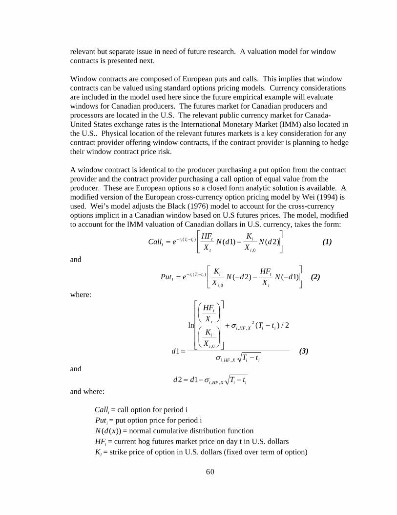
60

relevant but separate issue in need of future research. A valuation model for window contracts is presented next. Window contracts are composed of European puts and calls. This implies that window contracts can be valued using standard options pricing models. Currency considerations are included in the model used here since the future empirical example will evaluate windows for Canadian producers. The futures market for Canadian producers and processors are located in the U.S. The relevant public currency market for Canada-United States exchange rates is the International Monetary Market (IMM) also located in the U.S.. Physical location of the relevant futures markets is a key consideration for any contract provider offering window contracts, if the contract provider is planning to hedge their window contract price risk. A window contract is identical to the producer purchasing a put option from the contract provider and the contract provider purchasing a call option of equal value from the producer. These are European options so a closed form analytic solution is available. A modified version of the European cross-currency option pricing model by Wei (1994) is used. Wei’s model adjusts the Black (1976) model to account for the cross-currency options implicit in a Canadian window based on U.S futures prices. The model, modified to account for the IMM valuation of Canadian dollars in U.S. currency, takes the form:

Call eHFX

N dKX

N dir T t t

t

i

i

i i i= −⎡

⎣⎢

⎤

⎦⎥− −( )

,

( ) ( )1 20

(1)

and

Put eKX

N dHFX

N dir T t i

i

t

t

i i i= − − −⎡

⎣⎢

⎤

⎦⎥− −( )

,

( ) ( )0

2 1 (2)

where:

d

HFX

KX

T t

T t

t

t

i

i

i HF X i i

i HF X i i

1

2

0

2

=

⎛⎝⎜

⎞⎠⎟

⎛

⎝⎜

⎞

⎠⎟

⎡

⎣

⎢⎢⎢⎢⎢

⎤

⎦

⎥⎥⎥⎥⎥

+ −

−

ln ( ) /

,

, ,

, ,

σ

σ (3)

and d d T ti HF X i i2 1= − −σ , ,

and where:

Calli = call option for period i Puti = put option price for period i N d x( ( )) = normal cumulative distribution function HFt = current hog futures market price on day t in U.S. dollars Ki = strike price of option in U.S. dollars (fixed over term of option)

61

X t = current exchange rate in U.S. dollars to buy 1 Canadian dollar (IMM definition)

X i ,0 = delivery exchange rate in U.S. dollars to buy 1 Canadian dollar (pre-specified and fixed over term of option)

T ti i− = time to expiration of option (T=date of expiration, t=date of calculation)

σ σ σ ρσ σi HF X i HF i X i i HF i X, , , , , ,= + −2 2 2 = standard deviation of returns on Canadianized futures price

σi HF,2 =CME hog futures variance of returns calculated in this study using 58 day

historical estimate from market close to close σi X,

2 = Currency exchange rate variance of returns calculated in this study using 58 day historical estimate from market close to close data

ρi = correlation coefficient between futures and spot exchange rate for period I using 58 day historical returns.

ri = risk free interest rate (relevant Canadian T-Bill rate for this study). The difference between these formulas and the standard Black (1976) model is the inclusion of currency conversions and the volatility measure that incorporates the variance of returns on the foreign future commodity price, the variance on the currency and the correlation between the commodity futures and the currency. The strike prices are also converted to Canadian dollars at the time the option is opened and the strike price remains fixed for the remainder of the option period. The correlation coefficient is subtracted (versus added) when the domestic currency is priced in the foreign currency. The window valuation model uses the option formulas in the following manner. A floor price, which is a put option strike price, is chosen. Put option premiums can be calculated using the put model. This requires the standard inputs on volatility (standard deviation of returns), domestic interest rates, current commodity futures prices, exchange rates and time to maturity of the option (Hull 1993). Equating the put option premium to the call option premium, the condition for the window to have zero value when initiated, allows one to numerically calculate the ceiling price, which is the call strike price. Thus, the window has zero value and a price window between the put strike and the call strike. In this particular model, the strike prices are in Canadian dollars to account for the cross currency nature of the futures markets available to Canadian producers or processors. This type of valuation model avoids the ad hoc valuation approach practiced at the present time in the hog industry and represents a reasonable model for ensuring that both parties enter into a contract that has zero initial value. A critical issue remaining to be addressed is the determination of the price window for short term windows.

5.2. ESTABLISHING THE PRICE WINDOW FOR SHORT TERM CONTRACTS

The major issue with short-term and long-term window contracts is where to establish the floor and ceiling prices. Selection of the price window for existing industry contracts has

62

often been arbitrary with floor and ceiling prices chosen symmetrically around some predetermined cash price or around the futures price. This hog industry practice does not guarantee that the contract has zero value when opened. The modified Black pricing model proposed above requires that either the floor price or the ceiling price must be specified before the window contract can be valued. The location of the price window determines the risk characteristics of the contract. Selection of the price window is not a trivial issue. Two methods for determining the price window are proposed here. The first method uses a projected break-even price to determine the price floor of the window contract. The second method uses estimates of a confidence interval on the expected futures price at window contract expiry. The lower bound on the confidence interval is used to determine the price floor. A break-even price is a natural selection for a price floor in the window contract. The producer or the contract provider calculate the expected break-even price for the commodity to be protected using a window contract. An arbitrary adjustment to the break-even, for example subtracting C$0.05/kg. from the break-even price, could also be incorporated in a livestock commodity. In this case, the producer or contract provider is choosing a maximum acceptable loss. This choice determines the put strike price. Determination of the call strike value follows. Numerically, it is easily demonstrated that the futures price is not half way in between the put strike and the call strike with this price window. This provides justification for avoiding zero initial value window contracts where the difference between the floor price and the futures price is somewhat arbitrarily set equal to the difference between the futures price and the ceiling price. One serious problem arises when determining price windows using break-even analysis. Periodically, the window is inverted. That is, the call strike price is lower than the put strike price. This situation arises when the current futures price is below the adjusted break-even price. When this occurs, the necessary put option is in the money. Window valuation method selects a call option that is also in the money. Thus, an inverted window is created. Empirical work indicates this occurs often in the hog industry however no empirical work has yet been conducted for the beef industry. This result is not surprising considering the conclusions of Koontz et al. (1992) that distant futures contracts traded at approximately average cost of feeding levels, in other words around break-even levels. The empirical effectiveness of short term contracts has been explored in detail for the Canadian pork industry. These results as well as the model for estimating the confidence interval are available from the researchers.

5.3. LONG TERM WINDOW AND SPREAD CONTRACTS

Finance theory provides a method for valuing long term commodity contingent claims. The finance literature is already addressing this valuation issue for non-agricultural commodities (Schwartz, 1997, Gibson and Schwartz 1990, 1991). A critical component in valuing long term commodity contingent claims, the specification of the price distributions, are analyzed. This is less of an issue in the short term contracts specified

63

above. The type of distribution or the existence of price reversion (Irwin, Zulauf and Jackson 1996; Schwartz 1997) has a major impact on the pricing and viability of any long-term window contracts. A random walk and a mean reverting price process for live cattle, feeder cattle, lean hogs, corn and soybean meal prices are evaluated. Option valuation theory will be combined with the price distributions to give valuation examples of cost-plus and window contracts for hogs and live cattle. Results from the hog industry have applications to the future contracting arrangements in the beef industry. Two types of long term contracts are examined. These are cost-plus contracts and window contracts. Lawrence and Wang (1997) discuss various versions of cost-plus contracts for the pork industry. Generally the minimum price is tied to the feed costs, typically corn and soybean meal prices. The minimum price rises as feed costs rise and declines as feed prices drop. The processor makes up the difference when market livestock prices are below the minimum price. The producer often makes up the price difference when market prices rise by some fixed amount over the minimum contract price. Often the feed prices are averaged over part of the production period for the animals marketed on that contract. Ad hoc adjustments to the contract are used in the pork industry and are often included in the contract to prevent one party benefiting tremendously to the detriment of the other party. For example, if one party has accrued a large dollar surplus by the end of the contracting period as a result of the contract, the counter party may elect to extend the contract period. As discussed later, the cost-plus contract is essentially a contract on producer margins or spreads, the difference between the input costs and the output price. These contracts manage the risk between changes in input and output prices. Window contracts provide a minimum floor price and a maximum ceiling price to the producer as discussed above. Many different risk-sharing agreements are possible with a window contract or with a cost-plus contract. Window contracts are strictly a contract on the market price and only manage the output price risk from the producer perspective or the input price risk from the processor perspective. Conceptually both window contracts and cost-plus contracts can be decomposed into portfolios of options. Windows contracts are the simplest of the two products to explain using finance terminology. Algebraically the producer pay off at delivery of the finished product for production period extending from time t to T with a window contract is described as:

Farm Payoff S Max X S Max S Xt T T L T T U , [ , ] [ , ]= + − − −0 0 (4) where ST is the market price at delivery, XL is the fixed floor price and XU is the fixed ceiling price where usually XL < XU. Max X SL T[ , ]− 0 is the terminal put payoff to the producer and Max S XT U[ , ]− 0 is the terminal call payoff to the processor. If the market price is below the floor price (ST<XL) at delivery the producer price is ST plus the maximum of X SL T− or 0. Thus, the pay off is S X ST L T+ − which means the farm gets the floor price XL. Similarly if ST>XL then the farm payoff is the ceiling price XL. If X S XL T U< < then the farm receives the prevailing market price, ST. Equation 4 defines

the pay off diagram shown in Figure 4.

64

To have a valid price window, the put strike price, XL, must be less than the call strike, XU. Notice that the ceiling and floor prices are fixed (non-stochastic) and that the window contract is only concerned with the market price of the commodity being sold by the supplier. The cost of production is not included in the contract and if there is a significant change in the cost of production, this is not covered by the window contract. Conceivably, the break even cost of production price could be well outside the price window established at the beginning of the contract. As discussed by Unterschultz et al. (1997), placing the window around or above the break even price may not allow the contract to be rationally valued when the break even is above prevailing futures market prices Cost-plus contracts, or margin/spread contracts to be more exact, can also be decomposed into portfolios of specialized puts and calls and eliminate problems with determining the location of the window on window contracts. For simplification we assume here that the cost-plus contract has an upper bound beyond which the process does not have to pay the market price. Without an upper bound, the processor has a large liability with no direct offsetting benefit. The options to be discussed next are related to exchange or spread options, the ability to exchange one asset for another asset. (Margrabe 1978, Shimko 1994). Shimko (1994) describes spread options as an option on a portfolio that is long one asset and short another. With the cost-plus price contract the producer buys a spread put and sells a spread call. These spread options are based on the difference between input market prices such as soybean meal and corn, and output market prices. This spread option is conceptually easily adapted to the processor livestock input price and wholesale output price. Analytically, the terminal farm payoff appears similar to the window contract but has several major differences in the definition of the terms. The analytical terminal payoff for production period from time t to T is:

Farm Payoff S Max K S Max S K Ct T T L tI

T T L tI , , ,[ , ] [ ( ), ]= + − − − +0 0 (5)

where ST is the market output price at delivery, KL tI, is the minimum floor price and C is

some fixed dollar amount agreed to in the contract. KL tI, is stochastic since it is a function

of input prices and varies with time. For example, following Lawrence and Wang (1997) KL t

I, is calculated as a function of average corn prices and soybean meal prices during

part of the production period6. The fixed constant C limits the liability of the processor offering such contracts. Max K SL t

IT[ , ], − 0 is the terminal spread put payoff to the

producer and Max S K CT L tI[ ( ), ],− + 0 is the terminal spread call payoff to the processor.

If the market price is below the floor price S KT L tI< , at delivery the producer price is ST

6 Lawrence and Wang (1997) for hogs use an eight week rolling average on soybean meal and corn. The inputs are 350 pounds of feed (80% corn and 20% soybean meal) per cwt. of hog marketed plus other costs of $35/ton of feed, $14/cwt of animal sold and an additional $5/cwt as part of the “plus”. This forms the function for the minimum price

(i.e. KL tI, ). The maximum price (i.e. C) is adjusted upward by setting C=$5/cwt.

65

plus the maximum of K SL tI

T, − or 0. Thus, the pay off is S K ST L tI

T+ −, which means the

farm gets the minimum price, KL tI, which is a function of production costs (i.e. the farmer

does not exchange the stochastic input value for the stochastic output price). Similarly if S K CT L t

I> +, then the farm payoff is the ceiling price K CL tI, + which is a function of

production costs and some fixed amount above the fixed price. If K S K CL tI

T L tI

, ,< < + then the farm receives the prevailing market price, ST. Again, these options are not exercised until maturity, making them European. Both window contracts and cost plus contracts can be decomposed into portfolios of puts and calls. In theory these puts and calls can be valued. However, several valuation constraints exist with long term contracts that are lessor issues with shorter term contracts. A key input or assumption to value these contracts is the stochastic process used for the price distribution. This topic is addressed next.

5.4. STOCHASTIC PROCESSES FOR LONG TERM CONTRACTS

Option models are used to value puts and calls. The window contract is composed of simple options on the market output price. The modified Black (1976) model (equations 1, 2 and 3) used to value these window contracts requires that the underlying asset price follow a log normal stochastic process (i.e. the short term asset returns are a random

walk: dSS

dt dz= +α σ where S is the asset price, α is the non stochastic drift rate

(trend), σ is the non stochastic instantaneous variance and dz is brownian motion.). The cost-plus contract is composed of options on the spread between input prices and output prices. Since spread values can become negative and two or more stochastic variables are in the option, the Black model is not suitable for valuing these contracts. Presumably these spread variables are related both in theory and in practice. If these variables are co-integrated then this should imply that there are bounds on the value of the spread options even if the individual prices appear to be non-stationary. Several valuation issues for these long term options arise. These are:

• What is the most appropriate stochastic price process to use (i.e. are the price processes stationary or non-stationary)? • What type of models are required given the stochastic price process? • What input variables should be used for long term contracts since futures prices, the preferred input price, in general do not trade beyond two years into the future? • How can the model be tested or evaluated to determine if the calculated prices are reasonable when markets for these contracts do not yet exist?

The finance literature is addressing many of these issues for non-agricultural commodities (Schwartz, 1997; Gibson and Schwartz 1990 1991; Brennan 1991; Shimko 1994) and we address the first three issues. Irwin, Zulauf and Jackson (1996), using seventeen years of data, conclude statistically that prices for corn, soybeans, wheat, live

66

hogs and live cattle do not have mean-reversion. This suggests that a log normal distribution may be suitable even for valuing these long term contracts. However Pindyck and Dixit (1994, p.78) assert that using only 30 or so years of data, it is difficult to distinguish between a random walk verses a mean reverting process. Thus they recommend that the individual use theoretical considerations (i.e. equilibrium mechanisms in the sector) to determine whether mean-reverting price processes are appropriate. In particular commodity prices should revert to long run marginal costs7. Schwartz (1997) examines several different reverting models for non-agricultural commodities and concludes that the reversion parameters are significant. Two different price processes are compared. The first process assumes that all the prices follow a log-normal price process. That is:

dS S dt S dz i l ji i i i i i= + =α σ ... (6) where S is the spot price for commodity i, α is the drift rate (expected rate of return in a risky world), dt is the time increment, σ is the standard deviation of the process (volatility), dzi is standard normal brownian motion and ρij is the correlation between dzI and dzj. Volatilities and correlations are estimated using simple daily returns. The second process assumes a mean reverting process following model 1 in Schwartz (1997). This process is:

dS k S S dt S dz i jordX k X dt dz

i i i i i i i

i i i i i i

= − + =

= − +

( ln( )) ...)

( )

µ σ

α σ

equivalently by setting X = ln(Si i

1 (7)

where k measures the degree of reversion to long run mean log price α i . This process has a simple discrete version for parameter estimation. Parameters are derived by estimating the model:

X a b X ei t i i i t i i, , )= + + =−12 where Var(ei σ (8)

The Schwartz model and the log normal model are simplified here by assuming the Capital Asset Pricing Model provides an adequate measure of the market price for risk. Further details are in Schwartz (1997). The data used to estimate the parameters for the different price processes are discussed next.

5.5. DATA DESCRIPTION AND ANALYSIS OF LONG TERM CONTRACTS

Futures price series for live cattle (Chicago Mercantile Exchange-CME), feeder cattle (CME), lean hogs (CME) corn (Chicago Board of Trade-CBOT) and soy bean meal (CBOT) are evaluated. Bridge-CRB provided the futures data. The nearby futures contracts were spliced together to provide a proxy measure for the prevailing daily or 7 Other models may suggest that prices are discontinuous at certain times. This can be modeled as a jump process (Hull 1993, pp.442-443). Jorion (1989) concludes that exchange rates, a possible component of the models discussed here, exhibit discontinuities that should be modeled. This issue is not explored any further here.

67

monthly cash prices for each of these commodities. Although more data are available, the data analyzed covered the period January 1987 to December 1997 (i.e. 11 years of data). The US CPI index was used to deflate the price series when inflation adjusted analysis was performed. The S&P 500 index was used for estimating CAPM. Future analysis could easily incorporate exchange rate considerations and applied work evaluating forward contracts on Canadian wheat have included the currency. The Western Barley Futures contract on the Winnipeg Commodity Exchange was not used since it has less liquidity than the corn futures contract. Generally, currency risk is of less concern in these models. Currency considerations can be easily added in the future to price these models if required and generally commodities and currency have a zero correlation. Daily returns data were generated and used to develop preliminary estimates of the volatilities and correlations for log normal prices. These are used to evaluate short-term parameter stability. Following Hull (1993), ninety days of market prices (not adjusted for inflation) were used for each estimate. To analyze the eleven years of data, a rolling analysis that continually added one trading day while dropping the oldest (91st) trading day was performed. The results are reported in Table 5.1. The volatilities, converted to an annual basis, show a wide variation over the time period. For example, corn's volatility ranges from 0.09 to 0.50. Lean hogs are the most volatile and feeder cattle are the least volatile with annualized standard deviations of 0.26 and 0.12 respectively. The simple 90 day correlations reported in 2- 2 demonstrate similar variability. Feeder cattle and corn correlation ranges from -0.59 to 0.31 with a mean of 0.05. Other commodities exhibit similar ranges in correlation estimates. These results indicate that future work incorporate changing volatilities or correlations. Seemingly unrelated regressions (SUR) estimation was used on equation (8) for all five commodities to estimate volatilities, correlations, log of the long run mean and reversion parameters. The results for the correlations and volatilities are reported in 5.3. Estimates using price data adjusted for inflation were also included to evaluate differences in parameter estimates. These are also found in Table 5.3. The correlation and volatility estimates are similar to the estimates discussed above. For simplicity, the Table 5.3 results are used in the simulations reported below for window contracts and spread contracts. The important correlations to note are the small relationship between lean hogs and corn/soybean meal. Feeder cattle are more highly correlated to corn and live cattle. While not formally tested, this suggests a stronger equilibrium relationship in the cattle complex. The reversion parameters, reported in Table 5.4, are the annual rate of reversion (ki) to the long run log of the mean (α i ). Lean hogs exhibit the strongest reversion parameter, 1.99, when estimated using data not adjusted for inflation. The log of the long run mean for lean hogs is 4.17 or approximately $64.5/cwt8. Schwartz (1997) has further details on 8 The instantaneous rate of reversion is approximately $9.55/cwt (annually) if the spot price is $60/cwt, the mean is $65/cwt and the reversion parameter is 1.99.

68

how these parameter estimates are related. Statistical significance of the results was not tested since the primary objective was to provide parameter estimates for mean reverting price distributions. To evaluate different model assumptions, both inflation adjusted and nominal parameter estimates are used to simulate window and spread options. The beta CAPM estimates (Table 5.4) indicate that these commodities exhibit little systematic risk. These parameter estimates are used to evaluate pricing in window and spread contracts discussed next.

5.6. MONTE CARLO MODEL VALUATION OF LONG TERM CONTRACTS

Monte Carlo simulation techniques are used to value long term window and spread options on lean hogs and spread options on live cattle (i.e. finished beef animals). Details on the risk neutral stochastic price processes based on equations (6) and (7) used in the Monte Carlo are found in Hull (1993). Essentially, Monte Carlo techniques are used to simulate the potential price paths through time in a risk neutral world. The option value is calculated at the end of the price path and discounted at the risk free rate. This process is repeated many thousands of times to arrive at an initial option value. The market price of risk is required for these simulations and the risk free interest rate is assumed to be 7%. Future research can easily incorporate currency risk. Ten year contracts that covered production at 1 year, 1.5 years, 2 years, 2.5 years to 10 years were assumed. Weekly prices were simulated to represent the price paths for up to ten years into the future. That is, contract options values were calculated with one year to maturity, then a new set of price paths was generated for 1.5 years to calculate the option values at 1.5 years and so on. Prior to valuing window contracts and spread contracts, the difference between the random walk price process (equation 6) and the mean reverting process (equation 7) is illustrated. Using the parameter estimates from Tables 5.3 and 5.4 for lean hogs, (not adjusted for inflation), a single price process generating a random walk and a mean reverting process are given in Figure 5.5 (10 years) and Figure 5.6 (40 years). The same random process, a set of random price shocks, is used to simulate both series shown in Figure 5.5. Initially the random walk and the reverting process are similar, however the mean reverting process eventually returns to the mean. The random walk continues to wander. Both processes exhibit wide variations in price but the greatest variation is observed in the random walk. Figure 5.6 illustrates a different set of random events over 40 years. The same series of random shocks (i.e. news events, demand shocks, weather etc) generate the price movements for both price processes. This clearly illustrates how similar a random walk and a strong mean reverting process appear over shorter time intervals of ten to twenty years. This also illustrates the drawback to ad hoc price adjustments to window contracts as discussed by Lawrence and Wang (1997). Extending the term of the contract may not do anything to improve the cash position of one party relative to the counter party, especially if the price series exhibits the traits of a random walk. Similar albeit less dramatic results would occur for the feeder cattle and slaughter cattle parameters.

69

Long term window contracts for lean hogs (i.e. dressed weight) are simulated using the parameter estimates (adjusted for inflation). The reverting process assumes a mean of $75/cwt. The call and put strike prices are 80 and 70 respectively. The put and call premium could be equalized for each time to maturity by adjusting the strike prices for each specific maturity but this is not attempted here. Figures 5.7, 5.8, 5.9, 5.10, and 5.11 illustrate options premiums ranging from one to 10 years in maturity for hogs and cattle. Figure 5.8 illustrates option premium for live cattle similar to the assumptions used in Figure 5.7. Figure 5.9 illustrates the option premium for feeder cattle similar to the assumptions used in Figure 5.7. The option values based on the random walk (non-reverting process) illustrate how much more valuable the implicit price floors and price ceilings are in window contracts. Figure 5.7 shows that choosing a window where the floor price is an equally distant from the current price as the ceiling price does not result in a “fair” window value if prices follow a random walk. A "fair" window would have the put premium equal the call premium at each maturity date such that there is no net benefit to either the producer or the processor when the contract is signed. The reverting process shows that the call option and the put option have almost equal value through out most of the time period. The most obvious difference is the much lower option values for the reverting process. Current prices $10/cwt above or below the long run mean (Figures 5.10 and 5.11) have little impact after year 2 on the option values generated using a mean reverting process. Different windows would be required for different times to maturity to provide a fair contract under the assumptions used to generate Figure 5.11. The impact of spot prices outside the range of the floor and ceiling price are quite large if the option premiums are generated using a random walk. Figure 5.12 demonstrates the impact of different levels of reversion on call option premiums. Even relatively lower levels of reversion cause major reductions in the value of long-term options. Similar results would be applicable to the beef industry as seen in Figures 5.8 and 5.9. These window contract results highlight several key points. Knowledge about the underlying price process is essential before entering into long term contracts. The price risks are substantial if prices during the period of the window contract exhibit traits similar to a random walk or if the price window is not correctly chosen. This in part explains the substantial benefits Lawrence and Wang (1997) show accruing to one party under their historical simulation for hog window contracts. Different strike prices may be required for different times to maturity if the value of the floor price (put option) is to equal the value of the ceiling price (call option). Window contracts can be fairly priced at the beginning, however under the random walk hypothesis, it is highly likely that one party will end up substantially ahead. With a mean reverting process, if the mean is correctly identified and the floor and ceiling prices correctly placed then the window contract option values are smaller and current deviations of the spot price from the long run mean have little impact on option values expiring after two years. The key point here is to correctly identify the mean and then determine the price window under the reverting process hypothesis.

70

Next lean hog spread contracts were simulated using the parameter estimates for corn, soybean meal and lean hogs reported in Tables 5.3 and 5.4 (not adjusted for inflation). Similar production relationships between corn, soybean meal and hogs presented by Lawrence and Wang (1997) are used to estimate the spread floor. These are:

• 0.78 converts live weight to carcass • 400 total pounds of feed per cwt. live weight • 0.8 portion of feed that is corn • 0.2 portion of soybean meal in feed • 35/ton of feed and 14/cwt of animal are other costs • 8.0/cwt live weight cost plus in the contract for the spread ceiling • Spot price equal to the mean at the time 0

Spread contracts for lean hogs are illustrated in Figure 5.13. Under a random walk two facts are immediately evident. The cost plus factor of $8 is too low given the parameters and production assumptions. The option premiums are still substantial when compared to the option premiums simulated using the mean reverting process. Option premiums when the price processes follow a reverting process and the "true" parameters are known are much smaller. A similar spread option for live cattle (finished cattle) is simulated based on live cattle, feeder cattle and corn prices using Tables 5.3 and 5.4 values (not adjusted for inflation). As demonstrated below, the higher correlations between the cattle complex versus the lean hog spread have a major impact on the option values. Again a very simple production function is used for illustrative purposes. This function is:

• 7=feed conversion rate i.e. 7 lbs. of feed for 1 lb. of gain • 1.09 =conversion on corn price to get cost of ration consumed • 800=feeder cattle incoming weight (lbs.) • 1200=finished live weight (lbs.) • 3=rate of daily gain (i.e. 3lb/day) • 0.2=yardage charge per day per animal • 28= other fixed cost such as buying=5, trucking=3, deathloss=10, processing=3 veterinary=7 • 20=cost plus amount per animal • Spot price equal to the mean at the time 0

The live cattle spread contract is illustrated in Figure 5.14 and assumes the spot price is at the mean. Despite the smaller volatilities associated with cattle prices versus hog prices, the reverting price process has higher spread option values for cattle. This result appears to be driven by the larger absolute values on the correlations between live cattle, feeder cattle and corn returns. Figure 5.15 further highlights this point for the call values on the spread. The model where all price reversions and correlations are zero is similar to the premiums when the reversion is non-zero but correlations are also non-zero. Small spread option values only occur when the correlations are set to zero. The larger non-zero correlations in the cattle spread result in relatively higher spread option premiums

71

and counter part of the impact of the reversion parameter. Further simulations, not shown here, indicate the key correlation driving this result is the negative correlation between corn and feeder cattle returns. That is, the reversion parameter is less important for spread options where the prices appear to be co-integrated. These spread contract simulations highlight several key points about cost plus contracts. The choice of the production relationship and the size of the cost plus are critical to the success of these contracts. The correlations can have a very important impact on the option value and hide the impact of any reversion component on the spread option value. The implied option values in cost plus contracts can be substantial. Equalizing the value of the put spread and the call spread may require that the cost plus component be adjusted for different times to maturity.

5.7. MATH MODELS AND WINDOW CONTRACT CONCLUSIONS

Window contracts are a new and growing OTC price risk tool in the hog industry. Applications to the beef industry would use similar mathematical and numerical models. These instruments provide a mechanism which protects users partly from decreasing market prices but provides greater flexibility in gaining from upward market moves than hedging or forward contracts. Window contracts can be priced as a portfolio of long European puts and short European calls using special combinations of standard option models. Short-term window contracts are not without their problems. Selection of the price floor and ceiling is not a trivial issue. The relationship between futures prices and production costs are such that a short-term window contract that will guarantee no losses cannot always be offered. The window becomes inverted and realistically the producers must remain without a contract or possibly resort to other instruments such as put contracts. Basing the choice of price floor on the possible low realizations from the distribution of futures prices -- the confidence interval method -- is an alternative method of the designing the short-term window contract to alleviate the inverted window problem. While the contracts have attractive risk management features, study of this specification reveals another fundamental problem with short-term window contracts. The window widths vary extensively over time, the price floor moves with changing price conditions, and the risk properties of the contract change with this variation. Thus, short-term window contracts produce more volatile price protection than their long-term -- several years in length -- counter parts. Commodity pricing contracts are being used for managing risk in long term producer-processor contracting relationships. These contracts include long-term window contracts and cost plus contracts. These contracts can be also be decomposed into portfolios of puts and calls. With the cost-plus price contract the producer buys a spread between input prices and output price and sells a spread between input prices plus cost and output prices. These spread alternatives can be valued as puts and calls on the spread.

72

In theory these puts and calls can be valued. However, several valuation constraints exist with long-term contracts that are lessor issues with shorter term contracts. A key input or assumption to value these contracts is the stochastic process used for the price distribution. Window and spread contract values were simulated assuming either a random walk stochastic process or a mean reverting stochastic price process. A random walk process, a non-stationary series, can be difficult to distinguish from a stationary process, a mean reverting series. The different assumptions on the stochastic process have very different implications on the option values contained in window contracts and cost plus contracts. Mean reverting processes, where the mean is correctly identified, lead to lower valued implied options in both window and spread contracts. Different strike prices may be required for different times to maturity if the value of floor price (put option) is to equal the value of the ceiling price (call option) for window contracts. The floor and ceiling prices for window contracts and the cost plus portion of spread contracts need to change with the expected delivery date. Window contracts can be fairly priced at the opening of the contract, however under the random walk hypothesis, it is highly likely that one party will end up substantially ahead. With a mean reverting process, if the mean is correctly identified and the floor and ceiling prices correctly placed then the window contract appear to hold lower risk. Ad hoc adjustments to the contract may be required to keep the contract "fair" to all parties. These types of contracts may have relatively low use by the cattle industry. However, these models could be used to help set initial prices if parties enter into long term pricing arrangements. The arrangements will need to be periodically reviewed to make sure that both parties are satisfied with the arrangement. These tools can be used in conjunction with other risk management tools already available and with value-based-marketing.

73

Table 5.1. Simple 90 Day REturns Volatility Estimates for 1987-1997

Commodity Minimum Volatility

Maximum Volatility

Mean of 90 Day Volatilities

Mean Price1

soybean meal 0.09 0.47 0.21 $198.66/toncorn 0.09 0.50 0.21 2.57/bushellean hogs 0.15 0.41 0.26 65.11/cwt dressed feeder cattle 0.07 0.24 0.12 77.23/cwtlive cattle 0.09 0.24 0.15 70.89/cwt1. Price data is not adjusted for inflation.

Table 5.2. Simple 90 Day Returns Correlation Estimates for 1987-1997

Commodities Compared

Minimum Correlation

Maximum Correlation

MEAN of 90 Day Correlations

SBM-LC1 -0.33 0.43 0.01SBM-LH -0.51 0.48 0.07SBM-FC -0.57 0.25 -0.16SBM-C 0.13 0.84 0.56LC-LH -0.58 0.59 0.07LC-FC 0.18 0.89 0.57LC-C -0.41 0.40 0.02LH-FC -0.21 0.57 0.21LH-C -0.20 0.54 0.05FC-C -0.59 0.31 -0.181. SBM=Soybean Meal, LC=Live Cattle, FC=Feeder Cattle, LH=Lean Hogs, C=Corn

74

Table 5.3. Systems Estimates of Standard Deviations and Correlations Using Autoregressive Models

Commodity Soybean Meal

Corn Lean Hogs

Feeder Cattle

Live Cattle

Price Data Not Adjusted For Inflation Soybean Meal

1.00

Corn

0.54 1.00

Lean Hogs

0.16 0.16 1.00

Feeder Cattle

-0.27 -0.44 -0.01 1.00

Live Cattle -0.22 -0.19 -0.20 0.51 1.00

Std Dev. 0.18 0.21 0.23 0.10 0.13

Price Data Adjusted For Inflation Correlation Soybean

Meal Corn Lean

Hogs Feeder Cattle

Live Cattle

Soybean Meal

1.00

Corn

0.55 1.00

Lean Hogs

0.17 0.17 1.00

Feeder Cattle

-0.21 -0.38 0.03 1.00

Live Cattle -0.18 -0.16 -0.18 0.52 1.00

Std. Dev. 0.18 0.21 0.23 0.10 0.13

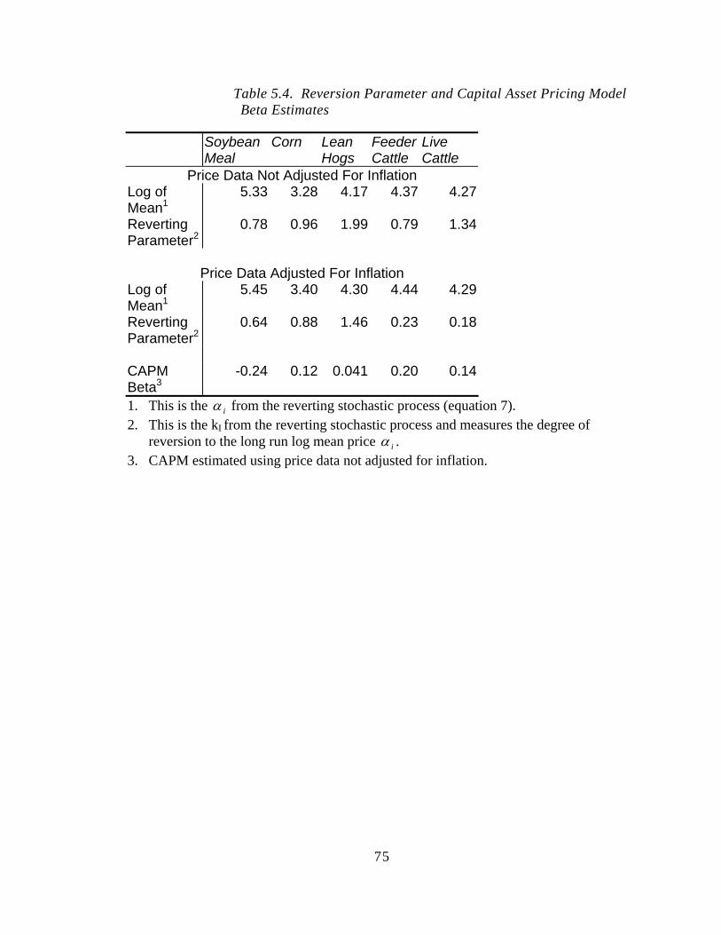
75

Table 5.4. Reversion Parameter and Capital Asset Pricing Model Beta Estimates

Soybean Meal

Corn Lean Hogs

Feeder Cattle

Live Cattle

Price Data Not Adjusted For Inflation Log of Mean1

5.33 3.28 4.17 4.37 4.27

Reverting Parameter2

0.78 0.96 1.99 0.79 1.34

Price Data Adjusted For Inflation

Log of Mean1

5.45 3.40 4.30 4.44 4.29

Reverting Parameter2

0.64 0.88 1.46 0.23 0.18

CAPM Beta3

-0.24 0.12 0.041 0.20 0.14

1. This is the α i from the reverting stochastic process (equation 7). 2. This is the kI from the reverting stochastic process and measures the degree of

reversion to the long run log mean price α i . 3. CAPM estimated using price data not adjusted for inflation.

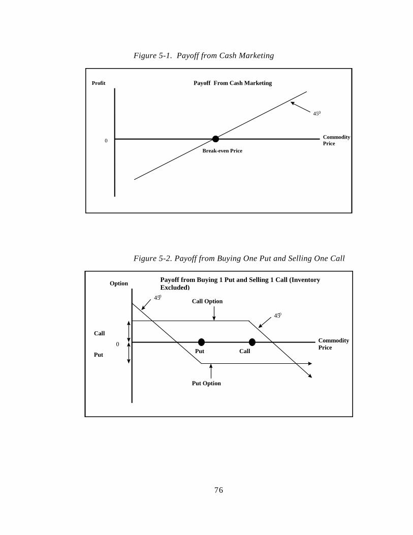
76

Figure 5-1. Payoff from Cash Marketing

Profit

CommodityPrice0

Payoff From Cash Marketing

Break-even Price

450

Figure 5-2. Payoff from Buying One Put and Selling One Call

Option

CommodityPrice0

Put Call

Put Option

Call Option

Payoff from Buying 1 Put and Selling 1 Call (InventoryExcluded)

Call

Put

450

450

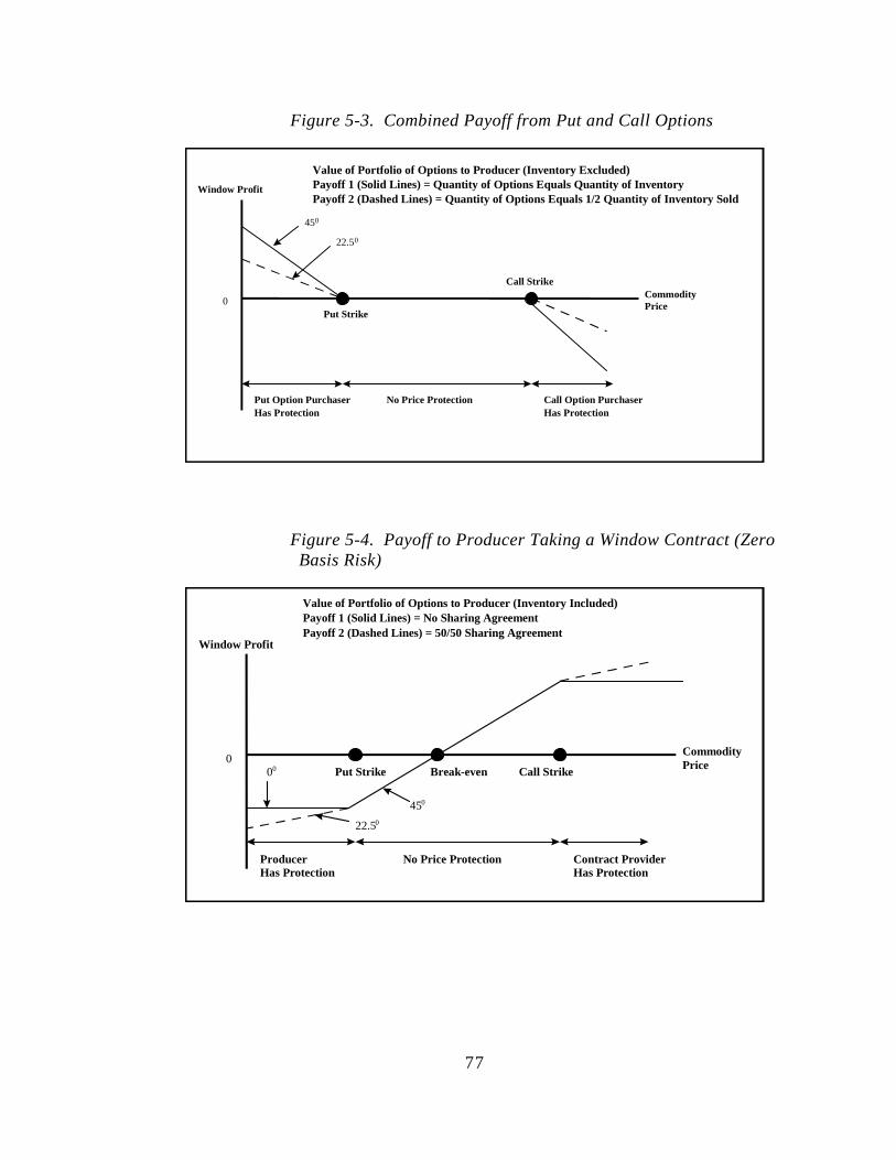
77

Figure 5-3. Combined Payoff from Put and Call Options

Window Profit

CommodityPrice0

Put Strike

Call Strike

Value of Portfolio of Options to Producer (Inventory Excluded)Payoff 1 (Solid Lines) = Quantity of Options Equals Quantity of InventoryPayoff 2 (Dashed Lines) = Quantity of Options Equals 1/2 Quantity of Inventory Sold

450

22.50

No Price ProtectionPut Option PurchaserHas Protection

Call Option PurchaserHas Protection

Figure 5-4. Payoff to Producer Taking a Window Contract (Zero Basis Risk)

Window Profit

CommodityPrice0

Put Strike Call Strike

Value of Portfolio of Options to Producer (Inventory Included)Payoff 1 (Solid Lines) = No Sharing AgreementPayoff 2 (Dashed Lines) = 50/50 Sharing Agreement

No Price ProtectionProducerHas Protection

Contract ProviderHas Protection

Break-even

450

22.50

00

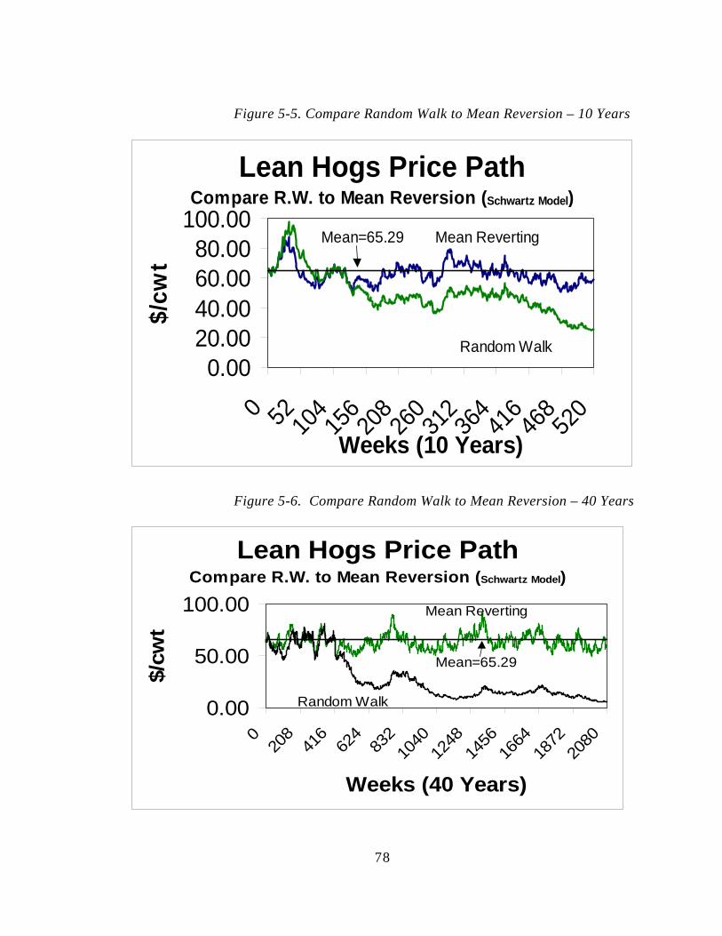
78

Figure 5-5. Compare Random Walk to Mean Reversion – 10 Years

Lean Hogs Price PathCompare R.W. to Mean Reversion (Schwartz Model)

0.0020.0040.0060.0080.00

100.00

0 52 104

156

208

260

312

364

416

468

520

Weeks (10 Years)

$/cw

t

Random Walk

Mean RevertingMean=65.29

Figure 5-6. Compare Random Walk to Mean Reversion – 40 Years

Lean Hogs Price PathCompare R.W. to Mean Reversion (Schwartz Model)

0.00

50.00

100.00

020

841

662

483

210

4012

4814

5616

6418

7220

80

Weeks (40 Years)

$/cw

t

Random Walk

Mean Reverting

Mean=65.29

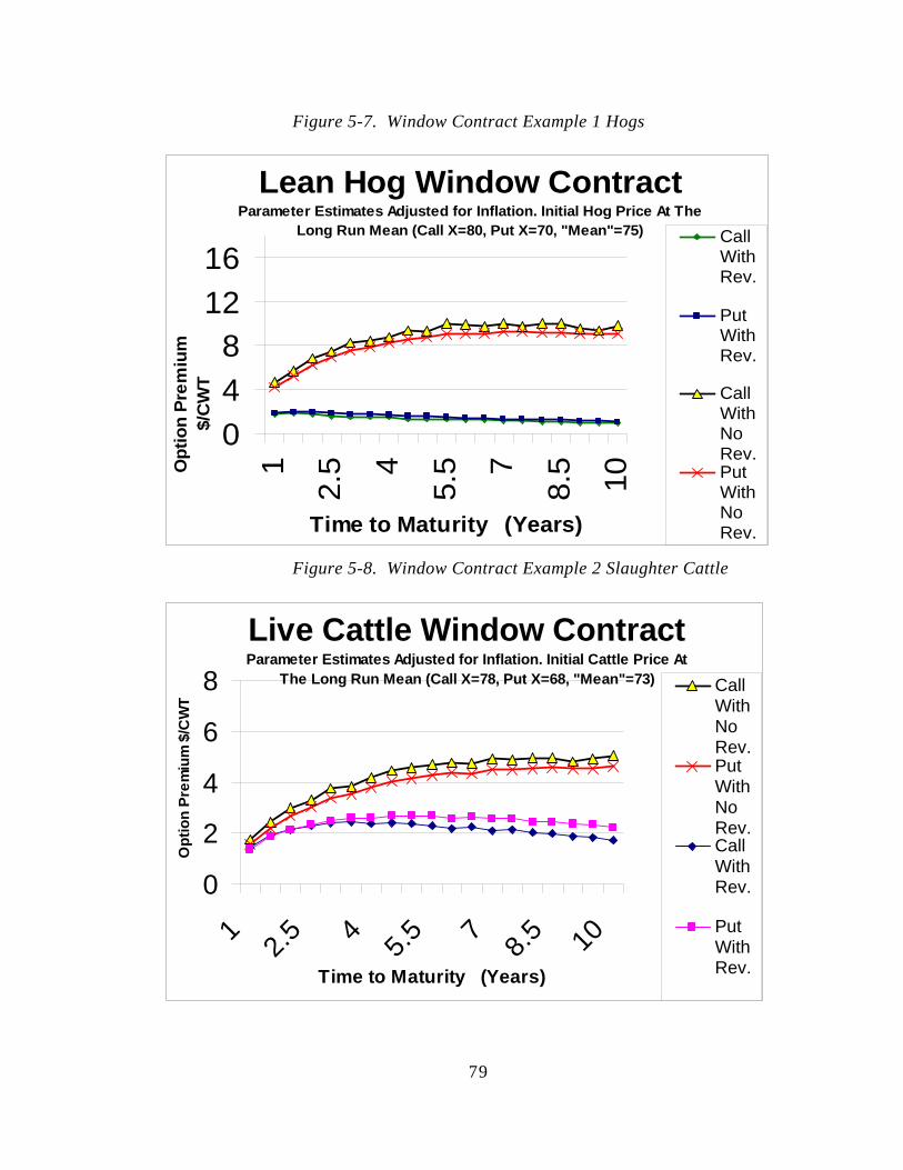
79

Figure 5-7. Window Contract Example 1 Hogs

Lean Hog Window ContractParameter Estimates Adjusted for Inflation. Initial Hog Price At The

Long Run Mean (Call X=80, Put X=70, "Mean"=75)

048

1216

1

2.5 4

5.5 7

8.5 10

Time to Maturity (Years)

Opt

ion

Prem

ium

$/

CW

T

CallWithRev.

PutWithRev.

CallWithNoRev.PutWithNoRev.

Figure 5-8. Window Contract Example 2 Slaughter Cattle

Live Cattle Window ContractParameter Estimates Adjusted for Inflation. Initial Cattle Price At

The Long Run Mean (Call X=78, Put X=68, "Mean"=73)

0

2

4

6

8

1 2.5 4 5.5 7 8.5 10Time to Maturity (Years)

Opt

ion

Prem

ium

$/C

WT

CallWithNoRev.PutWithNoRev.CallWithRev.

PutWithRev.

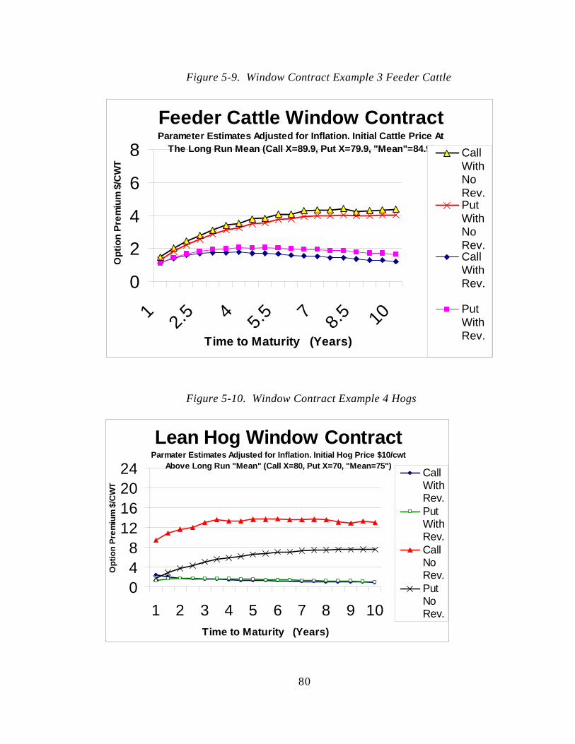
80

Figure 5-9. Window Contract Example 3 Feeder Cattle

Feeder Cattle Window ContractParameter Estimates Adjusted for Inflation. Initial Cattle Price At

The Long Run Mean (Call X=89.9, Put X=79.9, "Mean"=84.9)

0

2

4

6

8

1 2.5 4 5.5 7 8.5 10Time to Maturity (Years)

Opt

ion

Prem

ium

$/C

WT

CallWithNoRev.PutWithNoRev.CallWithRev.

PutWithRev.

Figure 5-10. Window Contract Example 4 Hogs

Lean Hog Window ContractParmater Estimates Adjusted for Inflation. Initial Hog Price $10/cwt

Above Long Run "Mean" (Call X=80, Put X=70, "Mean=75")

048

12162024

1 2 3 4 5 6 7 8 9 10Time to Maturity (Years)

Opt

ion

Prem

ium

$/C

WT

CallWithRev.PutWithRev.CallNoRev.PutNoRev.

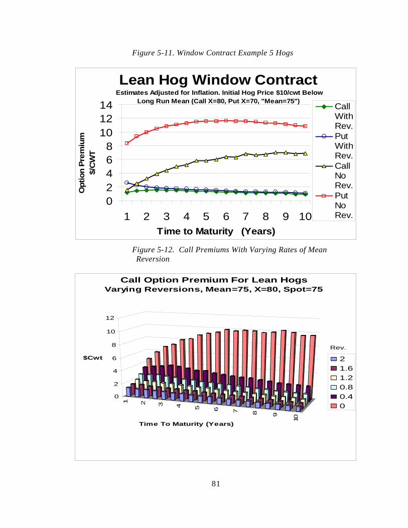
81

Figure 5-11. Window Contract Example 5 Hogs

Lean Hog Window Contract Estimates Adjusted for Inflation. Initial Hog Price $10/cwt Below

Long Run Mean (Call X=80, Put X=70, "Mean=75")

02468

101214

1 2 3 4 5 6 7 8 9 10Time to Maturity (Years)

Opt

ion

Prem

ium

$/

CW

T

CallWithRev.PutWithRev.CallNoRev.PutNoRev.

Figure 5-12. Call Premiums With Varying Rates of Mean Reversion

1 2 3 4 5 6 7 8 9

10

0

2

4

6

8

10

12

$Cwt

Time To Maturity (Years)

Call Option Premium For Lean HogsVarying Reversions, Mean=75, X=80, Spot=75

21.61.20.80.40

Rev.

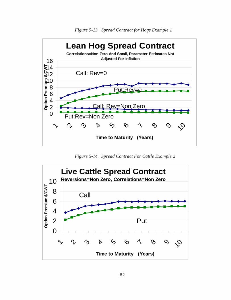
82

Figure 5-13. Spread Contract for Hogs Example 1

Lean Hog Spread ContractCorrelations=Non Zero And Small, Parameter Estimates Not

Adjusted For Inflation

02468

10121416

1 2 3 4 5 6 7 8 9 10Time to Maturity (Years)

Opt

ion

Prem

ium

$/C

WT

Call: Rev=0

Put:Rev=0

Call: Rev=Non Zero

Put:Rev=Non Zero

Figure 5-14. Spread Contract For Cattle Example 2

Live Cattle Spread ContractReversions=Non Zero, Correlations=Non Zero

02468

10

1 2 3 4 5 6 7 8 9 10Time to Maturity (Years)

Opt

ion

Prem

ium

$/C

WT

Call

Put

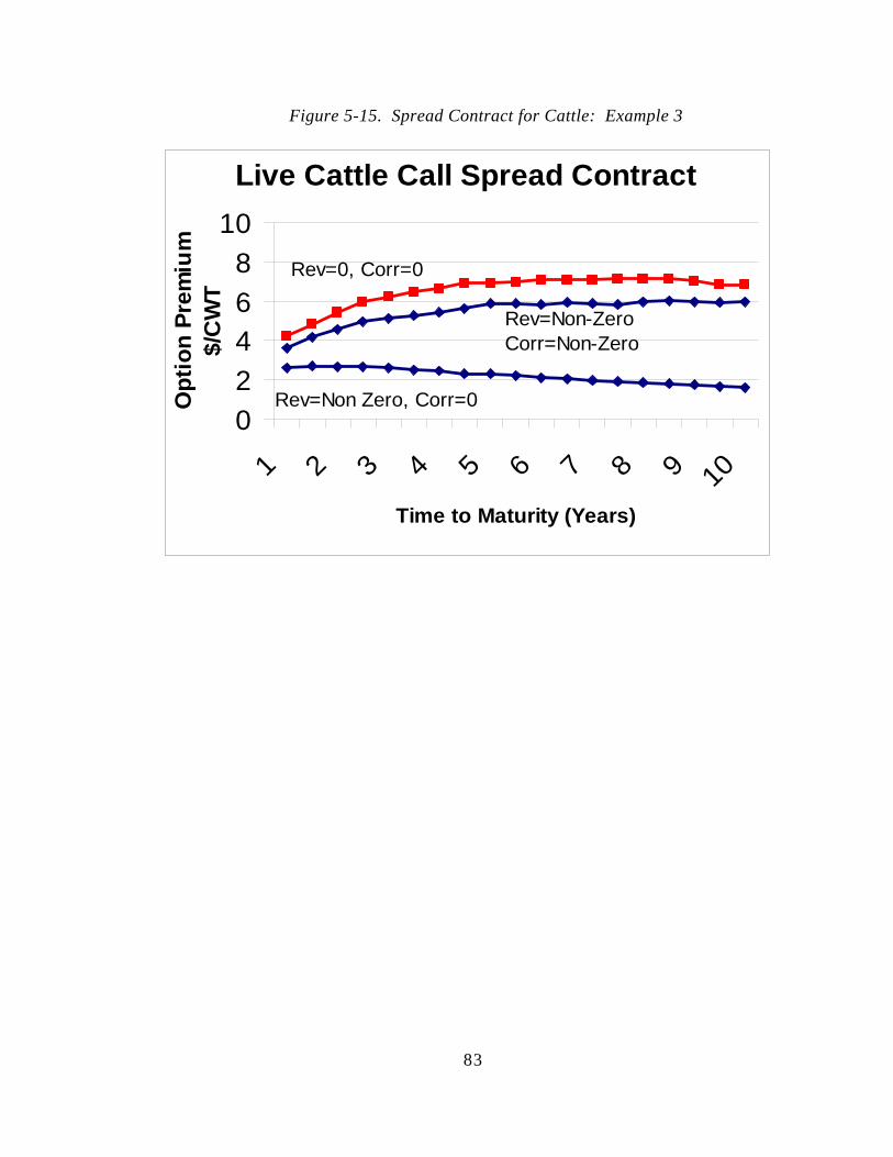
83

Figure 5-15. Spread Contract for Cattle: Example 3

Live Cattle Call Spread Contract

02468

10

1 2 3 4 5 6 7 8 9 10Time to Maturity (Years)

Opt

ion

Prem

ium

$/

CW

T

Rev=Non-ZeroCorr=Non-Zero

Rev=Non Zero, Corr=0

Rev=0, Corr=0

84

6. VARIABILITY IN VALUE-BASED MARKETING: RISK SHARING IN THE ALBERTA BEEF INDUSTRY

In the past few decades beef’s share of the total Canadian market has fallen considerably. Today, beef represents only 40% of total meat consumed by Canadian households. The expansion of the pork and poultry industries is quite evident. Lately focus has shifted towards identifying losses in market share that are related to concerns with the quality of beef products and consumer tastes and preferences (Purcell 1998). Beef quality issues are central in pricing value to consumers. For cattle feeders the quality of beef products begins with the animal carcass. Capturing the informational content of carcass data has been the focus of a number of studies. In Alberta for instance, feedlot trials have tested electronic identification (EID) systems as a means of tracing individual carcass information back to cattle origin (Basarab et al 1997; Basarab, Milligan and Thorlakson 1997). An analysis of Value-Based-Marketing using research data is discussed in Section 6.

6.1. PRICING TO VALUE AND QUALITY RISK

6.1.1. CARCASS QUALITY

The popularity of crossbreeding systems in Alberta results in a feeder animals that are characterized by “extreme variation in size, muscling, growth potential and carcass composition” (Basarab et al 1997, p. 386). One method of overcoming this animal variability is through selective purchasing of feeder cattle types. For instance, incoming groups of cattle may be assembled into relatively even lots by frame size or breed predominance. Once cattle arrive at the feedlot, growth implant programs and pen sorts into distinct feeding groups are also used to overcome the problem of feeder cattle consistency. For the most part these methods rely heavily upon a visual assessment of the growth potential of feeder cattle. Despite attempts to sort incoming cattle and feed accordingly, considerable variation still exists in carcass yield, quality and end-value (Basarab et al 1997). This variation is transformed into lost revenue when cattle do not conform to what the consumer values. Losses due to non-conformance in weight and yield and finish in fed cattle are estimated to cost the Canadian beef industry about $43.31 per head (Canadian Beef Quality Audit 1996). Yield and finish are a function of the quality grade, lean meat yield, and muscle thickness. Over two-thirds of this loss is attributable to carcass weight disparities. These issues relate back to the yield and quality risk factors discussed in Section 2. Currently the industry targets carcass weights in the 600 to 800 pound range. As Table 6.1 highlights the mean of the weekly average carcass weight for steers over the past seven years (762 pounds) is very close to the upper bounds of the target range. For instance, steers “averaged” 821 pounds during one particular week. While the extremes

85

in carcass weights are apparent in the upper range of weekly slaughter weights the trend towards larger carcasses was also noted in a previous section (Figure 3.17). Heavy weight cattle that exceed these targets are discounted and represent a significant cost for producing such big carcasses. On average almost twenty-seven thousand head of slaughter steers and heifers were graded weekly in Alberta during the 1992 to 1998 time period. Over one-quarter (27.6%) of these carcasses graded out to Canada AAA specifications for marbling, the top end of the quality range. During this seven-year period the percentage of AAA carcasses ranged from a low of 5.6 per cent to 49.1 per cent of weekly slaughter. In total more than 77 per cent of these slaughter steers and heifers graded Canada AA or better on a weekly basis. Carcasses falling into the Canada A-grade categories are also assigned yield grades based on estimates for meat yield. Almost two-thirds (66.0%) of these A-grade carcasses also produced top yield grades – Canada A1. Over the seven-year period, the percentage of A1’s ranged from a low of 50 per cent to almost 82 per cent of weekly slaughter. The lowest relative variation of quality and yield grades is evident in the Canada AA and Canada A1 grade categories, with coefficient of variations of 0.0946 and 0.0907, respectively.

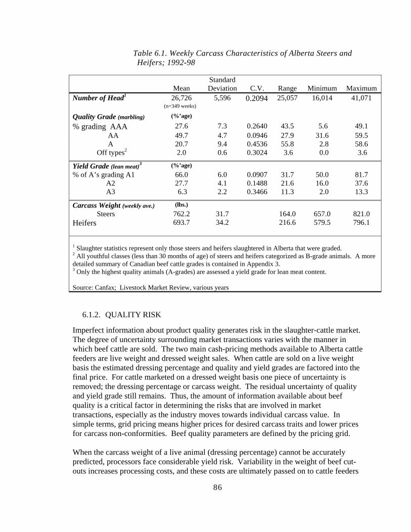
86

Table 6.1. Weekly Carcass Characteristics of Alberta Steers and Heifers; 1992-98

Mean

Standard Deviation

C.V.

Range

Minimum

Maximum

Number of Head1 26,726 5,596 0.2094 25,057 16,014 41,071 (n=349 weeks) Quality Grade (marbling) (%’age) % grading AAA 27.6 7.3 0.2640 43.5 5.6 49.1

AA 49.7 4.7 0.0946 27.9 31.6 59.5 A 20.7 9.4 0.4536 55.8 2.8 58.6 Off types2 2.0 0.6 0.3024 3.6 0.0 3.6

Yield Grade (lean meat)3 (%’age) % of A’s grading A1 66.0 6.0 0.0907 31.7 50.0 81.7

A2 27.7 4.1 0.1488 21.6 16.0 37.6 A3 6.3 2.2 0.3466 11.3 2.0 13.3

Carcass Weight (weekly ave.) (lbs.) Steers 762.2 31.7 0.0418 164.0 657.0 821.0

Heifers 693.7 34.2 0.0494 216.6 579.5 796.1 1 Slaughter statistics represent only those steers and heifers slaughtered in Alberta that were graded. 2 All youthful classes (less than 30 months of age) of steers and heifers categorized as B-grade animals. A more detailed summary of Canadian beef cattle grades is contained in Appendix 3. 3 Only the highest quality animals (A-grades) are assessed a yield grade for lean meat content. Source: Canfax; Livestock Market Review, various years

6.1.2. QUALITY RISK

Imperfect information about product quality generates risk in the slaughter-cattle market. The degree of uncertainty surrounding market transactions varies with the manner in which beef cattle are sold. The two main cash-pricing methods available to Alberta cattle feeders are live weight and dressed weight sales. When cattle are sold on a live weight basis the estimated dressing percentage and quality and yield grades are factored into the final price. For cattle marketed on a dressed weight basis one piece of uncertainty is removed; the dressing percentage or carcass weight. The residual uncertainty of quality and yield grade still remains. Thus, the amount of information available about beef quality is a critical factor in determining the risks that are involved in market transactions, especially as the industry moves towards individual carcass value. In simple terms, grid pricing means higher prices for desired carcass traits and lower prices for carcass non-conformities. Beef quality parameters are defined by the pricing grid. When the carcass weight of a live animal (dressing percentage) cannot be accurately predicted, processors face considerable yield risk. Variability in the weight of beef cut-outs increases processing costs, and these costs are ultimately passed on to cattle feeders

87

in the form of lower live weight prices. To reduce or share this risk processors must find better ways to predict carcass traits or establish means of tracking animals from the kill floor through processing and fabrication.

6.1.3. FORMULA AND GRID PRICING

Formula pricing, as the name implies, establishes a transaction price based upon a formula or equation. Pricing slaughter cattle on a formula basis essentially means that some other external price is used as a reference for the price cattle are sold at (Ward, Feuz, and Schroeder 1998). Grid pricing is a refinement of the dressed weight sales method in that the price focus shifts from a pen of cattle to each animal in that specific pen. Rather than pricing to the average of the group, individual animals are priced relative to carcass traits on a predetermined grid. The primary interaction of the quality and yield grade defines a two-dimensional scale upon which to evaluate the carcass merit of individual slaughter steers and heifers (Lamb and Beshear 1998). A secondary constraint is the final carcass weight. This produces a price grid with a scale for carcass merit at the base weight classification. Additional discounts are applied to carcasses outside this allowance for over- and under-sized carcasses. Grid pricing most often uses a formula for establishing the base price with premiums paid for cattle with desired carcass weights, yield, and quality grades and discounts applied to carcasses which fail to meet predetermined targets. Grid PriceI,t = Base Pricet + Premiumst - Discountst The base price in this formula is often some representation of cash trade in the local market but terms can vary considerably between contracts and across different packers and does not preclude cattle feeders and packers from openly negotiating a price base. The premiums and discounts in the grid price may or may not be additive (Schroeder and Davis 1998). This depends upon individual packer pricing grids.

6.1.4. SUMMARY

Traditional forms of price risk will undoubtedly remain. Recent changes to the structure of the beef industry present more challenges and introduce more risk into the system. The demand for value-based beef products is likely to draw an even closer linkage between price and production risk. Consumers’ demands for specific meat quality traits have pressured the beef industry to adapt in order to remain competitive with the pork and poultry industries at the retail level. Quality traits can influence prices paid to processors directly, and ultimately the price received by cow-calf producers. The quantity and quality of information are key elements in this process of price discovery (Koontz and Purcell 1997)

88

Cattle feeders’ attitudes towards risk also vary. While some individuals seek the higher returns from grade-and-yield pricing, others are content to let the processor assume the risk of grading the cattle. A study by Feuz, Fausti, and Wagner (1995) provides evidence of this risk-return tradeoff in slaughter cattle marketing. Their results from 744 steer calves indicated that on average, net returns were higher using a grade-and-yield marketing approach in the U.S. As the level of uncertainty surrounding the beef product increased packers discounted the price offered to cattle feeders, in effect lowering the average returns. This is the price cattle feeders pay for lowering the variability of cattle revenues. Grading animals generally requires at least one day and moves the pricing point away from the feedlot. This delay in payment adds to the perceived risk facing many cattle feeders who either do not understand grade-and-yield pricing or cannot visualize quality as easily as they might say, with the grain they are feeding. Once the animal is removed from the feedlot there is little connection with the final product. Relating grade and yield characteristics to a “live animal” is by no means an exact science and is further complicated by the limited information flow from processors. Changes to the pricing and grading systems are a necessary component of improving the flow of information from consumers to the primary producer (Koontz and Purcell 1997). In an effort to make the pricing system even more value-based, the CME has been fine-tuning the live cattle futures contract to promote more consistency in the carcass equivalent of the live animal (Chicago Mercantile Exchange 1999). Ideally, premiums and discounts should be identical to market-based spreads. Currently the USDA-AMS is surveying packers on a weekly basis to establish a database of processor spreads for various carcass grades. Information channels must stress quality as well as quantity, and grading systems must be capable of distinguishing demand for various beef quality attributes.

6.2. ANALYSIS OF QUALITY RISK

Value-based marketing has been suggested by the beef industry, especially packers and cattle feeders, as one alternative to ensuring that consumer preferences for beef products are met. Traditional marketing methods largely rely on pricing slaughter cattle on the average traits of an entire pen of cattle. Pricing slaughter cattle in a value-based system rewards individual animals for the desired carcass traits while penalizing carcass non-conformities. Grid pricing has been suggested as one method of improving the information flow between producers and packers about consumer demand for beef quality attributes . Recent studies in the US have examined the risk-return tradeoff with grid pricing alternatives. More specifically, these studies have questioned whether or not potential returns increase as cattle feeders assume more risk from an individual animal carcass quality pricing point (Beshear and Trapp, 1997; Feuz, 1998). In addition, Feuz, Fausti and Wagner (1995) show that pricing accuracy increases as cattle pricing moves from live weight marketing to carcass based methods of sale.

89

The objectives of this next discussion are: 1) quantify the revenue variability differences arising from quality issues of pricing cattle using live weight, dressed weight or grid pricing methods; and 2) assess the economic signal from packers to cattle feeders when cattle are priced on the merits of individual carcass traits. These objectives were accomplished by comparing two separate feedlot trials in different time periods using Canfax slaughter cattle prices for live weight and dressed weight sales and a single pricing grid. The final grid price was a formula price using the cash market carcass (rail grade) price of the previous week as the base price. Gross revenue variability was measured from the mean and standard deviation of total revenue for the three groups of slaughter cattle from individual animal data; steers and heifers were analyzed separately. Only animals with a plant carcass weight and grade and yield data were utilized in the pricing simulation.

6.2.1. DATA DESCRIPTION

Data used in this study includes local Alberta slaughter cattle prices, live cattle futures prices, exchange rates, and Alberta beef carcass grading statistics. Daily, weekly, and monthly data were collected for the ten-year period 1989 to 1998 where available. In addition primary slaughter cattle data was obtained from an Alberta Agriculture field trial assessing the performance of electronic identification systems in improving the uniformity of carcass conditions in Alberta feedlots.

6.2.1.1. Futures Data and Alberta Slaughter Cattle Prices

The Alberta slaughter cattle cash price used in this analysis is the direct to packer sales price (f.o.b. the plant) as reported by Canfax. This price series is an average of weekly sales of grade A quality steers and heifers to Alberta packing plants. Daily futures prices, used in the calculation of historical volatility and local basis patterns, were obtained from Tick Data Inc. for all live cattle contracts traded on the Chicago Mercantile Exchange. Bank of Canada exchange rates for the spot Canadian dollar, used in converting US futures prices into Canadian dollar terms, were obtained from a data series maintained by the Economic Services Division (Alberta Agriculture, Food and Rural Development).

6.2.1.2. Feedlot/Carcass Data

Actual slaughter cattle data was obtained from two of three separate trials conducted to assess the performance of electronic beef identification systems (BIDS) in improving the uniformity of carcass condition (Basarab et al 1997; Basarab, Milligan and Thorlakson 1997). This research study was conducted in Alberta feedlots with carcass information collected over an eighteen month time period -- from September 1994 through August 1996 -- and is referred to in this paper as the BIDS data. Table 6.4 and Table 6.5 provide a description of the carcass characteristics of the slaughter cattle in the feedlot trials

90

while Table 6.6 through Table 6.13 outline the results from applying the pricing model for live weight, dressed weight, and grade and yield price simulations to the BIDS data.

6.2.2. ANALYSIS AND PRICING METHODS

Slaughter cattle prices are predominantly determined by one of the three methods; 1) live weight basis at the feedlot or packing plant, 2) on a carcass weight basis after the animals have been slaughtered, or 3) on a carcass grade and yield basis. The grade and yield basis defines the carcass merit of individual animals and is often referred to as grid pricing or value-based pricing. In essence packers begin with a profit margin (or processing cost) and translate this into a bid price for a group of cattle (Ward, Schroeder and Feuz, 1998). Each pricing method is similar in this fashion. Differences arise for cattle feeders in the level of risk and information that is available at the moment price is determined. The price aspect of the quality risk analyzed in this study is measured by the variability of gross revenues from slaughter cattle sales. Three methods of pricing cattle, as defined above, are examined across two feedlot trials. Gross revenue variability was emphasized since pen-level cost profiles were not collected as a part of the BIDS trials. Using the historical data collected on pen-level cattle sales and individual animal carcass traits traced through the BIDS data, the pricing model simulates gross revenue variability by keying on the actual slaughter date. The price applied to individual animals reflects local market conditions and feedlot sorting methods. The total revenue for trial animals was used to facilitate this comparison.

6.2.2.1. Live weight Pricing

In each of the two feedlot trials almost a third of the cattle had a live animal weight recorded either upon arrival at the packing plant or upon leaving the feedlot. These weights were used to simulate a live price for each animal, based on average pen characteristics and the weekly Alberta direct to packer slaughter cattle price (Canfax, 1994-96). The live value for each animal in the pen was established as the product of: Live ValueI,t = Live Weighti * Cash Pricet the live sale weight of an individual animal i and the weekly average cash price in week t. The cash price was established on the assumption that the required percentage of steers and heifers fit the target quality characteristics of a packing plant. The weekly average live weight price was then matched to the date of sale for “all pens” of cattle in that week. In reality, cattle feeders in Alberta may see a range of prices for different lots of cattle on any given day (Dunford 1996).

91

6.2.2.2. Dressed Weight Pricing

In the BIDS trials the packing plant carcass weights was the actual pay weight. For means of comparison only animals with recorded quality and yield grades were used in this analysis. A flat rail price was applied to an entire pen of cattle with discounts for non-conforming animals beyond plant specifications. The dressed value for each animal in the pen was established as the product of: Dressed ValueI,t = Dressed Carcass Weighti * Cash Pricet the warm carcass weight of an individual animal i and the weekly average cash rail grade price in week t. Similar to the live weight price above, the cash price was established on the assumption that a percentage of steers and heifers fell within packer specifications for quality and weight for a pen of cattle. The weekly average dressed weight price was then matched to the date of sale for “all pens” of cattle in that week.

6.2.2.3. Grid Pricing

Unlike the live weight and dressed weight pricing methods, grid pricing shifts the price focus from an entire group of cattle to each individual animal in a pen of cattle. Rather than pricing to the average of the group each animal is priced relative to its individual carcass merit on a predetermined grid. The grid value for each animal in the pen was established as the product of: Grid ValueI,t = Dressed Carcass Weighti * Grid Pricet the warm carcass weight of an individual animal i and the grid price on the sale date t. The final transaction price in this grid pricing analysis was determined from individual animal carcass merit using a “formula” to establish the base price from the previous weeks reported average dressed weight slaughter price for steers and heifers in Alberta. Premiums and discounts representative of typical industry price differentials – and not specific to any packer – for non-conforming animals for quality grades, yield grades, and off-weight carcasses were assumed to be additive and were calculated from data provided by Canfax in Basarab et al (1997). Table 6.2 is a summary of the premiums and discounts used for the pricing grid in this study. This establishes a matrix or two-dimensional pricing grid such as the example in Table 6.3 for steer carcasses. Additional discounts are applied for over- and under-weight carcasses and off-type grades.

92

Table 6.2. Grid Pricing Premiums and Discounts

Price Adjustment for: ( per cwt. Dressed )

Quality Grade (marbling): AAA, Prime + $12.00 AA Base A - $0.00 B1 - $10.00 B2 - $25.00 B3, B4 - $35.00 D1, D2, D3 - $65.00 D4 - $80.00

Yield Grade (lean meat): A1 Base A2 - $3.00 A3 - $10.00

Carcass Weight (lbs dressed): > 920 lbs. - $25.00 821 to 920 lbs. - $10.00 751 to 820 lbs. - $5.00 550 to 750 lbs. Base 465 to 549 lbs. ** - $4.00 < 465 lbs. - $5.00

** Heifers are not discounted in this weight range. Data source: Basarab et al, 1997

For instance, an AAA/A2 steer with a carcass weight of 825 pounds would be valued at the base price less $1.00 per hundredweight with the grid in Table 5 (base price plus $9 for an AAA/A2 carcass less $10 for being overweight = -$1). The pricing simulation is intended to show what the risk would have been using a similar price grid for rewarding individual carcass merit.

93

Table 6.3. Pricing Grid for Steers

YIELD GRADES Canada A1 Canada A2 Canada A3 QUALITY GRADES ( $ per cwt. dressed )

Canada AAA 12.00 9.00 2.00 Canada AA Base -3.00 -10.00 Canada A 0.00 -3.00 -10.00

OTHER GRADES CARCASS WEIGHTS

Canada B1 -10.00 550-750 lbs. Base Canada B2 -25.00 Less than 465 lbs. -5.00 Canada B3,B4 -35.00 From 465 to 550 lbs. -4.00 Canada D1,D2,D3 -65.00 From 750 to 820 lbs. -5.00 Canada D4 -80.00 From 820 to 920 lbs. -10.00

More than 920 lbs. -25.00

6.2.3. RESULTS

Actual data was obtained from three separate trials conducted to evaluate an electronic beef identification system (BIDS) for the Alberta beef industry. Sample data was analyzed from two of these trials involving 4,128 animals (Trial 1 = 1031 head and Trial 2 = 3097 head) placed on feed during the winters of 1994 and 1995. The data sets included 44 pens of cattle from three participating feedlots with individual records of live sale weight, warm carcass weight, yield and quality grades, pen sort, and date of sale.

6.2.3.1. Grade and Yield Data

The first trial examined 10 pens of steer calves sourced from local auction markets. These yearlings were placed in three feedlots across Alberta in the fall of 1994 and winter of 1995 and processed at the same packing plant over a twelve-month period. In general, the steer calves in this group entered the feedlots as relatively short-keep type cattle and were fed for a period of about 120 days on high-energy rations.

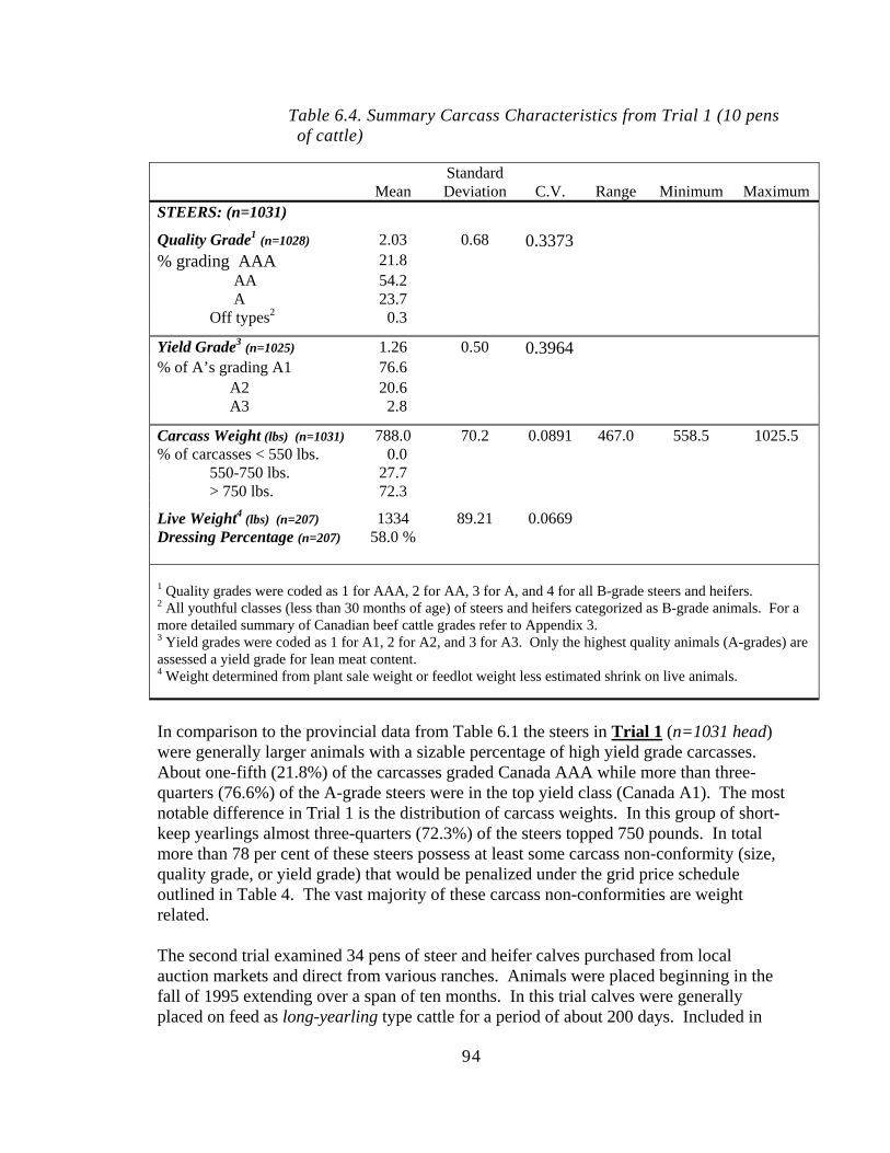
94

Table 6.4. Summary Carcass Characteristics from Trial 1 (10 pens of cattle)

Mean

Standard Deviation

C.V.

Range

Minimum

Maximum

STEERS: (n=1031)

Quality Grade1 (n=1028) 2.03 0.68 0.3373 % grading AAA 21.8

AA 54.2 A 23.7 Off types2 0.3

Yield Grade3 (n=1025) 1.26 0.50 0.3964 % of A’s grading A1 76.6

A2 20.6 A3 2.8

Carcass Weight (lbs) (n=1031) 788.0 70.2 0.0891 467.0 558.5 1025.5 % of carcasses < 550 lbs. 0.0

550-750 lbs. 27.7 > 750 lbs. 72.3

Live Weight4 (lbs) (n=207) 1334 89.21 0.0669 Dressing Percentage (n=207) 58.0 % 1 Quality grades were coded as 1 for AAA, 2 for AA, 3 for A, and 4 for all B-grade steers and heifers. 2 All youthful classes (less than 30 months of age) of steers and heifers categorized as B-grade animals. For a more detailed summary of Canadian beef cattle grades refer to Appendix 3. 3 Yield grades were coded as 1 for A1, 2 for A2, and 3 for A3. Only the highest quality animals (A-grades) are assessed a yield grade for lean meat content. 4 Weight determined from plant sale weight or feedlot weight less estimated shrink on live animals.

In comparison to the provincial data from Table 6.1 the steers in Trial 1 (n=1031 head) were generally larger animals with a sizable percentage of high yield grade carcasses. About one-fifth (21.8%) of the carcasses graded Canada AAA while more than three-quarters (76.6%) of the A-grade steers were in the top yield class (Canada A1). The most notable difference in Trial 1 is the distribution of carcass weights. In this group of short-keep yearlings almost three-quarters (72.3%) of the steers topped 750 pounds. In total more than 78 per cent of these steers possess at least some carcass non-conformity (size, quality grade, or yield grade) that would be penalized under the grid price schedule outlined in Table 4. The vast majority of these carcass non-conformities are weight related. The second trial examined 34 pens of steer and heifer calves purchased from local auction markets and direct from various ranches. Animals were placed beginning in the fall of 1995 extending over a span of ten months. In this trial calves were generally placed on feed as long-yearling type cattle for a period of about 200 days. Included in

95

this group were three pens of the ranch calves (n=257 head) from six different producers. Although the sample size was relatively small the data was used for a precursory analysis of the significance of herd of origin impacts. Trial 2 (n=3097 head) contains a mix of steers and heifers which in comparison to the provincial slaughter data were generally lighter, higher quality grading animals.

Steers In this trial steer calves represent about one-quarter of the calves on feed. Almost twenty-six per cent of these carcasses graded Canada AAA while more than one-half (54.8%) of the A-grade steers were Canada A1 yield carcasses. On a quality and yield grade basis this group is fairly comparable to provincial slaughter. On average steers dressed out at 665.5 pounds, more than one hundred pounds under the provincial slaughter. Almost 89 per cent of the steer carcasses fell within the 550 to 750 pound weight range. Only a small portion (8.3 %) actually topped 750 pounds. In fact the largest steer carcass was only 838 pounds. In total only 53 per cent of these steers are discounted for one or more non-conformities (size, quality grade, or yield grade) under the grid pricing format used in this study.

Heifers Heifers on feed in Trial 2 comprise the largest group of feeder cattle in either of the two trials. Forty-four per cent of the heifer carcasses graded Canada AAA while slightly less than one-half (47.0%) of the A-grade heifers produced top lean meat yields (Canada A1 carcasses). The significant number of high quality grading heifers is partially offset by this decline in carcass yield grades when compared to provincial slaughter data. Heifers in this trial averaged only slightly more than six hundred pounds (602.6 pounds) on a dressed weight basis, almost one hundred pounds under the weekly provincial average. More than 81 per cent of the heifer carcasses fell within the 550 to 750 pound weight range. Only a negligible amount (0.5 %) of the heifers topped 750 pounds while more than 18 per cent dressed out at less than 550 pounds. Despite the tradeoff between lighter weight, lower yielding carcasses and premium quality grading carcass traits (marbling), only 54 per cent of these heifers are discounted for one or more non-conformities.

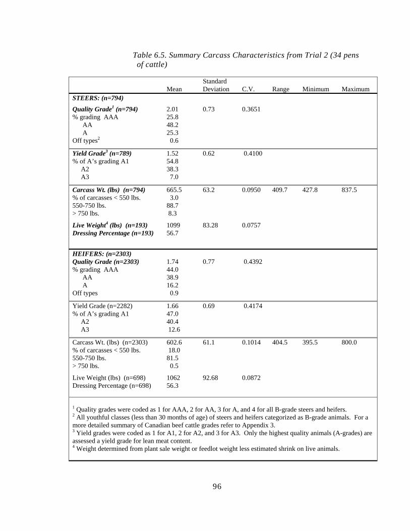
96

Table 6.5. Summary Carcass Characteristics from Trial 2 (34 pens of cattle)

Mean

Standard Deviation

C.V.

Range

Minimum

Maximum

STEERS: (n=794)

Quality Grade1 (n=794) 2.01 0.73 0.3651 % grading AAA 25.8 AA 48.2 A 25.3 Off types2 0.6

Yield Grade3 (n=789) 1.52 0.62 0.4100 % of A’s grading A1 54.8 A2 38.3 A3 7.0

Carcass Wt. (lbs) (n=794) 665.5 63.2 0.0950 409.7 427.8 837.5 % of carcasses < 550 lbs. 3.0 550-750 lbs. 88.7 > 750 lbs. 8.3

Live Weight4 (lbs) (n=193) 1099 83.28 0.0757 Dressing Percentage (n=193) 56.7

HEIFERS: (n=2303) Quality Grade (n=2303) 1.74 0.77 0.4392 % grading AAA 44.0 AA 38.9 A 16.2 Off types 0.9

Yield Grade (n=2282) 1.66 0.69 0.4174 % of A’s grading A1 47.0 A2 40.4 A3 12.6

Carcass Wt. (lbs) (n=2303) 602.6 61.1 0.1014 404.5 395.5 800.0 % of carcasses < 550 lbs. 18.0 550-750 lbs. 81.5 > 750 lbs. 0.5

Live Weight (lbs) (n=698) 1062 92.68 0.0872 Dressing Percentage (n=698) 56.3 1 Quality grades were coded as 1 for AAA, 2 for AA, 3 for A, and 4 for all B-grade steers and heifers. 2 All youthful classes (less than 30 months of age) of steers and heifers categorized as B-grade animals. For a more detailed summary of Canadian beef cattle grades refer to Appendix 3. 3 Yield grades were coded as 1 for A1, 2 for A2, and 3 for A3. Only the highest quality animals (A-grades) are assessed a yield grade for lean meat content. 4 Weight determined from plant sale weight or feedlot weight less estimated shrink on live animals.

97

6.2.3.1.1. Differences between Trials

The majority of slaughter animals in Trial 1 were identified as having some Continental breed influence. More than 47 per cent were Continental-British cross-bred steers. In contrast, Trial 2 was composed largely of lighter weight calves. More than one-half of these steers and heifers, 51.6 per cent and 56.9 per cent respectively, were identified as British breeds. No description of the type of cattle breed is available in provincial slaughter data for a comparison with the BIDS data. The most notable difference between the feedlot trials is the average slaughter weight and the relative distribution of dressed carcass weights. Trial 1 steers averaged almost 125 pounds more than the steers from Trial 2 on a dressed weight basis. Steers from the first trial were large yearlings placed on feed in the fall and winter on high-energy rations. This produced animals with higher slaughter end-weights. In contrast, the steers and heifers placed on feed in Trial 2 were lighter calves and yearlings, fed out to much lighter end-weights. On average these calves required an additional seventy-five to eighty days to reach a target sale weight. Since carcass weight stands out as a distinguishing feature between the two trials it is worth examining the weight distributions against the base weight classification for the pricing grid. Although the steers from Trial 1 are the most uniform group, only 27.7 per cent are within the base weight allowance. By comparison, well over 80 per cent of all steers and heifers from Trial 2 fit the base weight classification. More carcass weight means more revenue, all other things being equal. Live weight and dressed weight pricing methods tend to be much less restrictive on carcass size – average weight is the driving factor. Often carcasses have to exceed 900 pounds before individual animals are severely discounted. The pricing grid, on the other hand, discounts over-weight carcasses on an animal-by-animal basis, not by the average of a pen of cattle. A summary of carcass traits in Table 6.6 compares the relative variation across the three groups of cattle. The group of heifers in Trial 2 show the most relative variation in carcass weight while the 120-day fed steers from Trial 1 are the most uniform group of cattle. This pattern holds for the grade and yield data as well. These results highlight the distinction between the different types of cattle on feed in the two trials and the potential impacts from trying to value these animals on a grid.

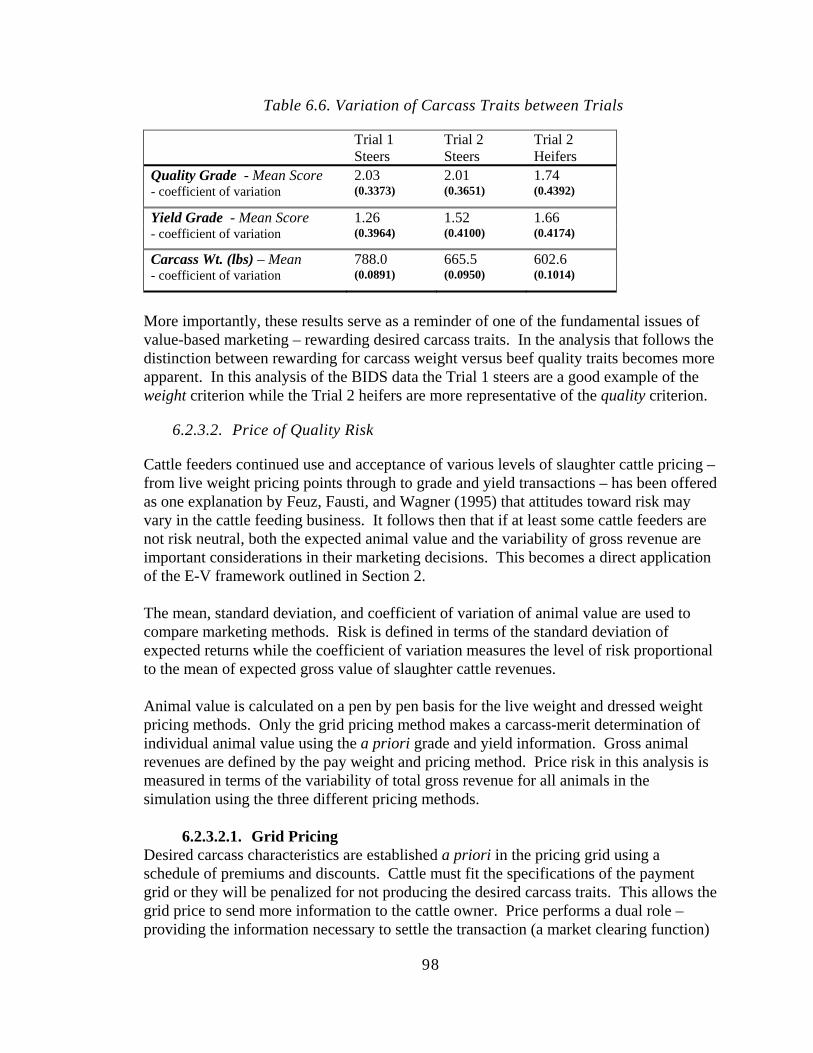
98

Table 6.6. Variation of Carcass Traits between Trials

Trial 1 Steers

Trial 2 Steers

Trial 2 Heifers

Quality Grade - Mean Score 2.03 2.01 1.74 - coefficient of variation (0.3373) (0.3651) (0.4392)

Yield Grade - Mean Score 1.26 1.52 1.66 - coefficient of variation (0.3964) (0.4100) (0.4174)

Carcass Wt. (lbs) – Mean 788.0 665.5 602.6 - coefficient of variation (0.0891) (0.0950) (0.1014)

More importantly, these results serve as a reminder of one of the fundamental issues of value-based marketing – rewarding desired carcass traits. In the analysis that follows the distinction between rewarding for carcass weight versus beef quality traits becomes more apparent. In this analysis of the BIDS data the Trial 1 steers are a good example of the weight criterion while the Trial 2 heifers are more representative of the quality criterion.

6.2.3.2. Price of Quality Risk

Cattle feeders continued use and acceptance of various levels of slaughter cattle pricing –from live weight pricing points through to grade and yield transactions – has been offered as one explanation by Feuz, Fausti, and Wagner (1995) that attitudes toward risk may vary in the cattle feeding business. It follows then that if at least some cattle feeders are not risk neutral, both the expected animal value and the variability of gross revenue are important considerations in their marketing decisions. This becomes a direct application of the E-V framework outlined in Section 2. The mean, standard deviation, and coefficient of variation of animal value are used to compare marketing methods. Risk is defined in terms of the standard deviation of expected returns while the coefficient of variation measures the level of risk proportional to the mean of expected gross value of slaughter cattle revenues. Animal value is calculated on a pen by pen basis for the live weight and dressed weight pricing methods. Only the grid pricing method makes a carcass-merit determination of individual animal value using the a priori grade and yield information. Gross animal revenues are defined by the pay weight and pricing method. Price risk in this analysis is measured in terms of the variability of total gross revenue for all animals in the simulation using the three different pricing methods.

6.2.3.2.1. Grid Pricing Desired carcass characteristics are established a priori in the pricing grid using a schedule of premiums and discounts. Cattle must fit the specifications of the payment grid or they will be penalized for not producing the desired carcass traits. This allows the grid price to send more information to the cattle owner. Price performs a dual role – providing the information necessary to settle the transaction (a market clearing function)

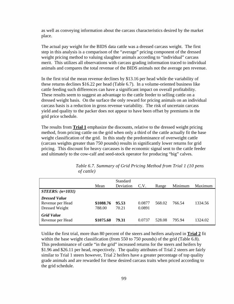
99

as well as conveying information about the carcass characteristics desired by the market place. The actual pay weight for the BIDS data cattle was a dressed carcass weight. The first step in this analysis is a comparison of the “average” pricing component of the dressed weight pricing method to valuing slaughter animals according to “individual” carcass merit. This utilizes all observations with carcass grading information traced to individual animals and compares the total revenue of the BIDS animals not the average pen revenue. In the first trial the mean revenue declines by $13.16 per head while the variability of these returns declines $16.22 per head (Table 6.7). In a volume-oriented business like cattle feeding such differences can have a significant impact on overall profitability. These results seem to suggest an advantage to the cattle feeder to selling cattle on a dressed weight basis. On the surface the only reward for pricing animals on an individual carcass basis is a reduction in gross revenue variability. The risk of uncertain carcass yield and quality to the packer does not appear to have been offset by premiums in the grid price schedule. The results from Trial 1 emphasize the discounts, relative to the dressed weight pricing method, from pricing cattle on the grid when only a third of the cattle actually fit the base weight classification of the grid. In this study the predominance of overweight cattle (carcass weights greater than 750 pounds) results in significantly lower returns for grid pricing. This discount for heavy carcasses is the economic signal sent to the cattle feeder and ultimately to the cow-calf and seed-stock operator for producing “big” calves.

Table 6.7. Summary of Grid Pricing Method from Trial 1 (10 pens of cattle)

Mean

Standard Deviation

C.V.

Range

Minimum

Maximum

STEERS: (n=1031) Dressed Value Revenue per Head $1088.76 95.53 0.0877 568.02 766.54 1334.56 Dressed Weight 788.00 70.21 0.0891

Grid Value Revenue per Head $1075.60 79.31 0.0737 528.08 795.94 1324.02

Unlike the first trial, more than 80 percent of the steers and heifers analyzed in Trial 2 fit within the base weight classification (from 550 to 750 pounds) of the grid (Table 6.8). This predominance of cattle “in the grid” increased returns for the steers and heifers by $1.96 and $26.11 per head, respectively. The quality attributes of Trial 2 steers are fairly similar to Trial 1 steers however, Trial 2 heifers have a greater percentage of top quality grade animals and are rewarded for these desired carcass traits when priced according to the grid schedule.

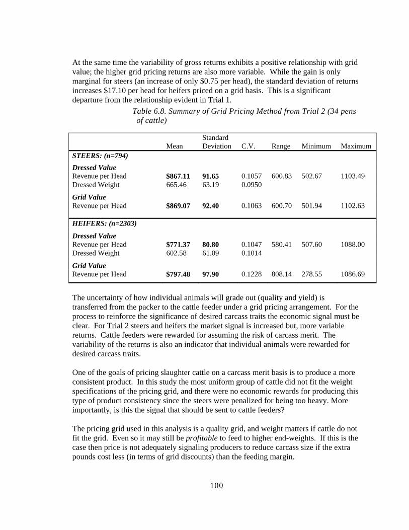
100

At the same time the variability of gross returns exhibits a positive relationship with grid value; the higher grid pricing returns are also more variable. While the gain is only marginal for steers (an increase of only $0.75 per head), the standard deviation of returns increases $17.10 per head for heifers priced on a grid basis. This is a significant departure from the relationship evident in Trial 1.

Table 6.8. Summary of Grid Pricing Method from Trial 2 (34 pens of cattle)

Mean

Standard Deviation

C.V.

Range

Minimum

Maximum

STEERS: (n=794) Dressed Value Revenue per Head $867.11 91.65 0.1057 600.83 502.67 1103.49 Dressed Weight 665.46 63.19 0.0950

Grid Value Revenue per Head $869.07 92.40 0.1063 600.70 501.94 1102.63

HEIFERS: (n=2303)

Dressed Value Revenue per Head $771.37 80.80 0.1047 580.41 507.60 1088.00 Dressed Weight 602.58 61.09 0.1014

Grid Value Revenue per Head $797.48 97.90 0.1228 808.14 278.55 1086.69

The uncertainty of how individual animals will grade out (quality and yield) is transferred from the packer to the cattle feeder under a grid pricing arrangement. For the process to reinforce the significance of desired carcass traits the economic signal must be clear. For Trial 2 steers and heifers the market signal is increased but, more variable returns. Cattle feeders were rewarded for assuming the risk of carcass merit. The variability of the returns is also an indicator that individual animals were rewarded for desired carcass traits. One of the goals of pricing slaughter cattle on a carcass merit basis is to produce a more consistent product. In this study the most uniform group of cattle did not fit the weight specifications of the pricing grid, and there were no economic rewards for producing this type of product consistency since the steers were penalized for being too heavy. More importantly, is this the signal that should be sent to cattle feeders? The pricing grid used in this analysis is a quality grid, and weight matters if cattle do not fit the grid. Even so it may still be profitable to feed to higher end-weights. If this is the case then price is not adequately signaling producers to reduce carcass size if the extra pounds cost less (in terms of grid discounts) than the feeding margin.

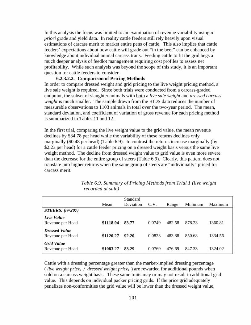
101

In this analysis the focus was limited to an examination of revenue variability using a priori grade and yield data. In reality cattle feeders still rely heavily upon visual estimations of carcass merit to market entire pens of cattle. This also implies that cattle feeders’ expectations about how cattle will grade out “in the beef” can be enhanced by knowledge about individual animal carcass traits. Feeding cattle to fit the grid begs a much deeper analysis of feedlot management requiring cost profiles to assess net profitability. While such analysis was beyond the scope of this study, it is an important question for cattle feeders to consider.

6.2.3.2.2. Comparison of Pricing Methods In order to compare dressed weight and grid pricing to the live weight pricing method, a live sale weight is required. Since both trials were conducted from a carcass-graded endpoint, the subset of slaughter animals with both a live sale weight and dressed carcass weight is much smaller. The sample drawn from the BIDS data reduces the number of measurable observations to 1103 animals in total over the two-year period. The mean, standard deviation, and coefficient of variation of gross revenue for each pricing method is summarized in Tables 11 and 12. In the first trial, comparing the live weight value to the grid value, the mean revenue declines by $34.78 per head while the variability of these returns declines only marginally ($0.48 per head) (Table 6.9). In contrast the returns increase marginally (by $2.23 per head) for a cattle feeder pricing on a dressed weight basis versus the same live weight method. The decline from dressed weight value to grid value is even more severe than the decrease for the entire group of steers (Table 6.9). Clearly, this pattern does not translate into higher returns when the same group of steers are “individually” priced for carcass merit.

Table 6.9. Summary of Pricing Methods from Trial 1 (live weight recorded at sale)

Mean

Standard Deviation

C.V.

Range

Minimum

Maximum

STEERS: (n=207) Live Value Revenue per Head $1118.04 83.77 0.0749 482.58 878.23 1360.81

Dressed Value Revenue per Head $1120.27 92.20 0.0823 483.88 850.68 1334.56

Grid Value Revenue per Head $1083.27 83.29 0.0769 476.69 847.33 1324.02

Cattle with a dressing percentage greater than the market-implied dressing percentage ( live weight pricei / dressed weight pricet ) are rewarded for additional pounds when sold on a carcass weight basis. These same traits may or may not result in additional grid value. This depends on individual packer pricing grids. If the price grid adequately penalizes non-conformities the grid value will be lower than the dressed weight value,

102

perhaps even lower than a live weight value. In this trial the significant number of non-conforming heavy-weight carcasses results in a negative grid-to-dressed difference. The relative variation of gross revenue declines when comparing the grid value to the live weight value for both trials. In the second trial the average of total revenue increases from $4.83 per head to $21.55 per head for steers and heifers respectively. Less than one-third of the cattle in Trial 2 (n=896 head) have a recorded live slaughter weight for steers and heifers (Table 6.10). The comparison of the three pricing methods draws from this subset.

Steers

In the second trial, comparing the live weight value to a grid value, the mean revenue increases by $21.55 per head while the variability of these returns increases by about $12.60 per head (Table 6.10). In contrast the returns decrease marginally (by $0.38 per head) for a dressed weight to live weight comparison. Overall, this translates into larger gains for a dressed to grid value comparison, and larger than the entire group of steers exhibited in Table 9.

Heifers Comparing the live weight value of heifers in Trial 2 to the grid value, the mean revenue increases by only $4.83 per head while the variability of these returns increases by more than $21.82 per head (Table 6.10). Dressed weight returns decrease significantly (by $17.30 per head) when compared to the live weight value. Again, this translates into larger gains for a dressed-to-grid value comparison. For heifers the gains are smaller than found in the entire group of heifers (Table 6.10). Looking at the minimum value for heifers under the grid price shows just how severe discounting can when animals are “individually” priced for carcass merit as opposed to “average” pricing methods.

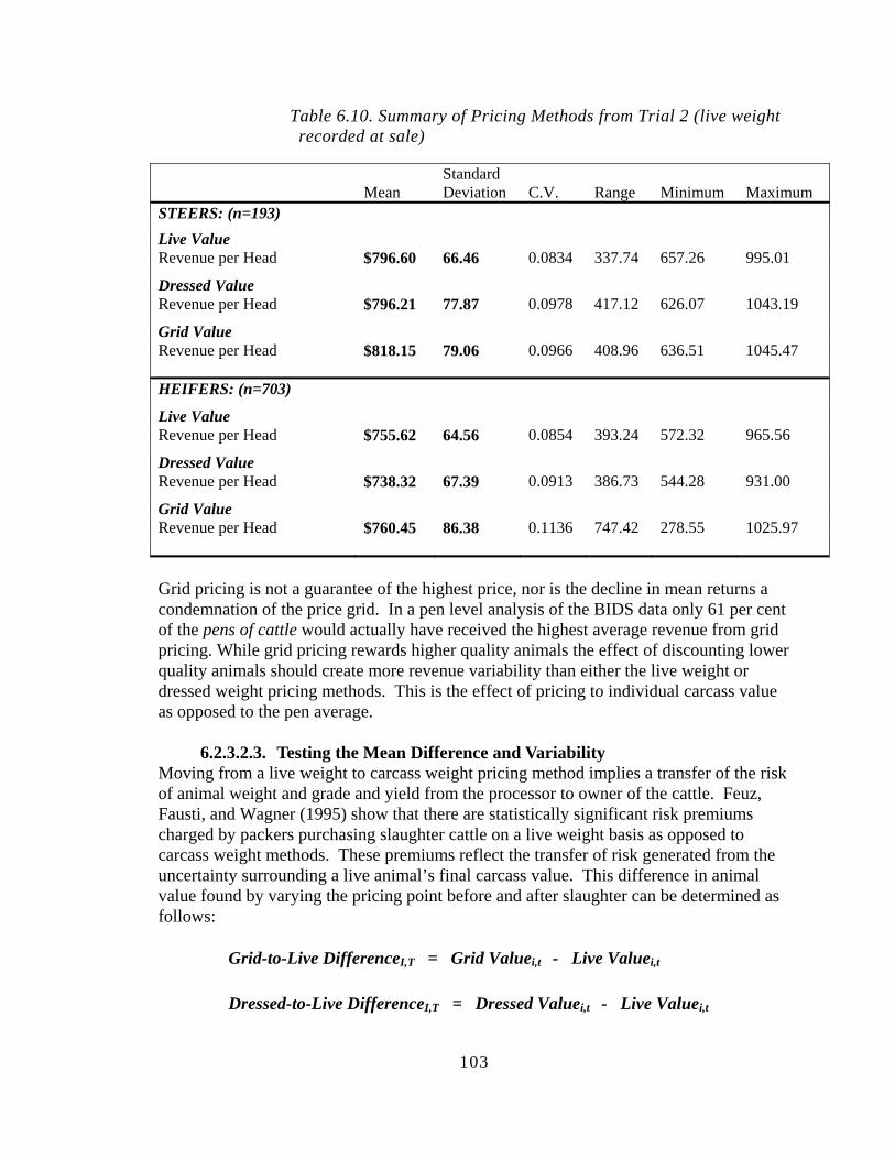
103

Table 6.10. Summary of Pricing Methods from Trial 2 (live weight recorded at sale)

Mean

Standard Deviation

C.V.

Range

Minimum

Maximum

STEERS: (n=193) Live Value Revenue per Head $796.60 66.46 0.0834 337.74 657.26 995.01

Dressed Value Revenue per Head $796.21 77.87 0.0978 417.12 626.07 1043.19

Grid Value Revenue per Head $818.15 79.06 0.0966 408.96 636.51 1045.47

HEIFERS: (n=703)

Live Value Revenue per Head $755.62 64.56 0.0854 393.24 572.32 965.56

Dressed Value Revenue per Head $738.32 67.39 0.0913 386.73 544.28 931.00

Grid Value Revenue per Head $760.45 86.38 0.1136 747.42 278.55 1025.97 Grid pricing is not a guarantee of the highest price, nor is the decline in mean returns a condemnation of the price grid. In a pen level analysis of the BIDS data only 61 per cent of the pens of cattle would actually have received the highest average revenue from grid pricing. While grid pricing rewards higher quality animals the effect of discounting lower quality animals should create more revenue variability than either the live weight or dressed weight pricing methods. This is the effect of pricing to individual carcass value as opposed to the pen average.

6.2.3.2.3. Testing the Mean Difference and Variability Moving from a live weight to carcass weight pricing method implies a transfer of the risk of animal weight and grade and yield from the processor to owner of the cattle. Feuz, Fausti, and Wagner (1995) show that there are statistically significant risk premiums charged by packers purchasing slaughter cattle on a live weight basis as opposed to carcass weight methods. These premiums reflect the transfer of risk generated from the uncertainty surrounding a live animal’s final carcass value. This difference in animal value found by varying the pricing point before and after slaughter can be determined as follows: Grid-to-Live DifferenceI,T = Grid Valuei,t - Live Valuei,t Dressed-to-Live DifferenceI,T = Dressed Valuei,t - Live Valuei,t

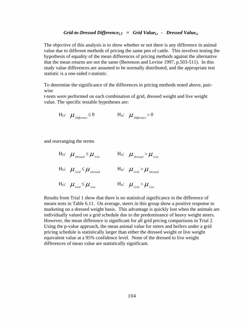
104

Grid-to-Dressed DifferenceI,T = Grid Valuei,t - Dressed Valuei,t The objective of this analysis is to show whether or not there is any difference in animal value due to different methods of pricing the same pen of cattle. This involves testing the hypothesis of equality of the mean differences of pricing methods against the alternative that the mean returns are not the same (Berenson and Levine 1997, p.503-511). In this study value differences are assumed to be normally distributed, and the appropriate test statistic is a one-sided t-statistic. To determine the significance of the differences in pricing methods noted above, pair-wise t-tests were performed on each combination of grid, dressed weight and live weight value. The specific testable hypotheses are: HO: 0≤µDifference

HA: 0>µDifference

and rearranging the terms HO: µµ LiveDressed

≤ HA: µµ LiveDressed>

HO: µµ DressedGrid

≤ HA: µµ DressedGrid>

HO: µµ LiveGrid

≤ HA: µµ LiveGrid>

Results from Trial 1 show that there is no statistical significance in the difference of means tests in Table 6.11. On average, steers in this group show a positive response to marketing on a dressed weight basis. This advantage is quickly lost when the animals are individually valued on a grid schedule due to the predominance of heavy weight steers. However, the mean difference is significant for all grid pricing comparisons in Trial 2. Using the p-value approach, the mean animal value for steers and heifers under a grid pricing schedule is statistically larger than either the dressed weight or live weight equivalent value at a 95% confidence level. None of the dressed to live weight differences of mean value are statistically significant.

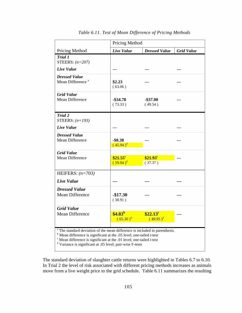
105

Table 6.11. Test of Mean Difference of Pricing Methods

Pricing Method

Pricing Method Live Value Dressed Value Grid Value Trial 1 STEERS: (n=207) Live Value --- --- ---

Dressed Value Mean Difference a $2.23 --- --- ( 63.06 )

Grid Value Mean Difference -$34.78 -$37.00 --- ( 73.33 ) ( 49.54 ) Trial 2 STEERS: (n=193) Live Value --- --- ---

Dressed Value Mean Difference -$0.38 --- --- ( 45.94 )d

Grid Value Mean Difference $21.55c $21.93c --- ( 59.04 )d ( 37.37 )

HEIFERS: (n=703)

Live Value --- --- ---

Dressed Value Mean Difference -$17.30 --- --- ( 38.91 )

Grid Value Mean Difference $4.83b $22.13c --- ( 65.30 )d ( 49.95 )d a The standard deviation of the mean difference is included in parenthesis. b Mean difference is significant at the .05 level; one-tailed t-test c Mean difference is significant at the .01 level; one-tailed t-test d Variance is significant at .05 level; pair-wise F-tests

The standard deviation of slaughter cattle returns were highlighted in Tables 6.7 to 6.10. In Trial 2 the level of risk associated with different pricing methods increases as animals move from a live weight price to the grid schedule. Table 6.11 summarizes the resulting

106

p-values from pair-wise F-tests comparing the differences in risk (standard deviation of returns) associated with the three pricing methods. In this trial the variability of grid value is not statistically different from the dressed weight value. However, the live weight value is different (p=0.0000). Although the grid pricing method exhibits higher variability in animal returns (standard deviation is 15% larger than dressed or live weight values), they are not statistically different from each other.

6.2.3.3. Genetic Factors

In both trials slaughter cattle revenues were analyzed across British, Continental, and British-Continental crosses of feeder calves. Table 6.12 summarizes these returns and the return variability of these animals by the identified breed type. Comparing the sample of slaughter animals with a recorded live weight reduced the number of observations by two-thirds. When this is taken in to account a balance between breed types is much more apparent between the two trials. In fact, the sample from Trial 1 reflects more of a British influence in the feeder calves (48.3 per cent British breeds versus 18.5 per cent for the entire group of steers). Revenues in Trial 1 decline by a large margin when comparing a live weight value to the grid- pricing alternative. British calves produce the highest average grid returns with the lowest decline from the live weight value ($26.37 per head). Continental breeds produce the largest live weight and dressed weight value, but suffer the largest loss when moving to a grid pricing arrangement. The decline of $52.55 per head represents a significant margin in cattle feeding. In general steers and heifers in Trial 2 exhibit increasing returns to selling on a grade and yield basis. The differences from grid to live weight values are larger among all slaughter animals. British-type heifers are the only exception and the decline is marginal. In the steer class, Continental type feeders exhibit the largest returns under all three pricing methods coupled with the highest variability of returns. For heifers, the British-Continental cross feeder produces the largest average return across all three pricing methods. The difference in heifer calves is less pronounced. No one type of cattle seems to provide superior returns to any method of pricing, least of all pricing on the grid. Cattle need to selected on the basis of fitting the grid in order to take full advantage of grid premiums for the carcass characteristics.

107

Table 6.12. Summary of Pricing Methods by Breed of Cattle

Live Value Dressed Value Grid Value Mean Std. Dev Mean Std. Dev Mean Std. Dev

TRIAL # 1 Steers: (n=207) British 48.3 % Revenue per Head $1115.85 83.96 $1120.20 85.07 $1089.48 80.41 Sale Weight (lbs.) 1349 93.19 781.00 55.12

Continental 28.5 % Revenue per Head $1131.15 78.64 $1134.09 102.99 $1078.60 85.39 Sale Weight (lbs.) 1334 81.82 781.64 60.09

British-Continental Cross 23.2 % Revenue per Head $1106.50 88.97 $1103.43 91.62 $1076.07 87.34 Sale Weight (lbs.) 1303 83.00 754.42 46.85

TRIAL # 2 Steers: (n=193) British 64.8 % Revenue per Head $796.39 65.07 $797.59 77.16 $817.82 79.09 Sale Weight (lbs.) 1097 80.39 622.53 50.28

Continental 7.3 % Revenue per Head $841.95 89.59 $861.71 95.10 $879.44 92.02 Sale Weight (lbs.) 1155 108.60 665.79 57.08

British-Continental Cross 28.0 % Revenue per Head $785.33 58.78 $776.05 65.31 $803.02 68.57 Sale Weight (lbs.) 1092 78.85 615.84 43.07

Heifers: (n=703)

British 59.9 % Revenue per Head $752.57 64.57 $734.85 67.81 $751.76 83.80 Sale Weight (lbs.) 1057 96.82 592.85 57.93

Continental 24.5 % Revenue per Head $760.05 67.30 $741.93 69.03 $770.94 88.97 Sale Weight (lbs.) 1073 87.87 608.29 54.86

British-Continental Cross 14.9 % Revenue per Head $762.23 60.08 $746.93 62.81 $779.12 88.94 Sale Weight (lbs.) 1067 82.09 603.00 52.79

108

6.2.3.4. Cattle Origin

The origin of cattle has been suggested as one factor influencing feedlot and carcass performance. In the second trial, a sample of heifer calves (n=77 head) was drawn from three lots of ranch calves, representing six different ranching operations. These heifers were the only ranch calves with both a recorded live slaughter weight and a final dressed carcass weight. As Table 6.13 indicates, heifer returns from the three pricing methods support the notion that ranch origin does make a difference.

Table 6.13. Summary of Pricing Methods by Cattle Origin (live weight recorded at sale)

Live Value Dressed Value Grid Value Mean Std. Dev Mean Std. Dev Mean Std. Dev

TRIAL # 2 Heifers: (n=77) Ranch #1 Revenue per Head $734.75 52.93 $706.50 43.05 $737.12 49.90 Sale Weight (lbs.) 1027 69.27 581.72 40.83

Ranch #2 Revenue per Head $718.38 53.84 $734.27 75.89 $744.28 72.96 Sale Weight (lbs.) 990 66.97 579.42 41.14

Ranch #3 Revenue per Head $748.02 71.02 $723.98 105.64 $745.57 107.23 Sale Weight (lbs.) 1028 99.42 566.90 81.85

Ranch #4 Revenue per Head $754.21 47.85 $750.52 48.12 $788.90 47.76 Sale Weight (lbs.) 1044 60.09 600.81 29.48

Ranch #5 Revenue per Head $796.06 50.67 $782.95 31.07 $832.87 56.77 Sale Weight (lbs.) 1105 69.73 632.90 42.27

Ranch #6 Revenue per Head $775.06 53.96 $762.29 62.67 $786.99 65.94 Sale Weight (lbs.) 1076 79.06 615.44 56.55 Returns were consistently higher for Ranch #5 and Ranch #4 across the three pricing methods. Less than 10 per cent of these heifers were discounted for non-conforming quality or yield characteristics and this is reflected in the total value of these animals. Furthermore, the variability of these returns is among the lowest of the group. Given this contrast it is worth examining the carcass characteristics of these heifers relative to grid parameters. Figures 6.1 to 6.4 highlight the grading performance with a comparison to provincial slaughter data.

109

Figure 6-1. Distribution of Heifer Quality Grades - Trial 2(a)

0%

10%

20%

30%

40%

50%

60%

70%

AAA AA A

Ranch 1 Ranch 2 Ranch 3 Alberta*

* per cent of total Alberta slaughter; 1994-1996

Figure 6-2. Distribution of Heifer Quality Grades - Trial 2(b)

0%

10%

20%

30%

40%

50%

60%

70%

AAA AA A

Ranch 4 Ranch 5 Ranch 6 Alberta*

* per cent of total Alberta slaughter; 1994-1996

110

Figure 6-3. Distribution of Heifer Yield Grades - Trial 2(a)

0%10%20%30%40%50%60%70%80%90%

100%

A1 A2 A3

Ranch 1 Ranch 2 Ranch 3 Alberta*

* per cent of total Alberta slaughter; 1994-1996

Figure 6-4. Distribution of Heifer Yield Grades - Trial 2(b)

0%10%20%30%40%50%60%70%80%90%

100%

A1 A2 A3

Ranch 4 Ranch 5 Ranch 6 Alberta*

* per cent of total Alberta slaughter; 1994-1996

From these distributions the relative performance of top quality cattle becomes more evident. The highest returns in general coincide with top quality animals fitting the base

111

weight range. The top two ranches have larger percentages of Canada AAA, A-1 carcasses and relatively few off-weight animals. Both distributions are skewed towards the premium quality animal. These results provide hints that more coordination between cow-calf producers, feedlots and packing plants could reduce yield and quantity risk. The financial benefits to the cow-calf producer will be highly dependent on the grid system used.

Figure 6-5. Distribution of Heifer Carcass Weights - Trial 2

0%

25%

50%

75%

100%

<550 lbs. 550-750 lbs. >750 lbs.

Ranch 1 Ranch 2 Ranch 3 Ranch 4 Ranch 5 Ranch 6

6.2.4. GRID PERFORMANCE

The pricing grid used in this analysis is a quality grid that rewards top quality animals within a specified weight range. Over- and under-weight carcasses are discounted. The variation in animal value in this study is based on variations in quantity (weight and dressing percentage), quality (lean meat yield and marbling grades), and the variation in prices offered at sale. One limitation of the BIDS data is that no price was collected at the point of sale; animals were sold on a dressed weight basis with all carcass data individually recorded. A model was used to simulate prices for live weight, dressed weight, and grade and yield revenues. Additional research measuring comparable bids for all three pricing methods at point of sale would be useful to assessing the significance of these findings. The most notable difference between the two trials is the opposite direction returns take when cattle are individually priced on a grid. Steers on feed in Trial 1 were larger yearlings that dressed out at much higher end-weights. The grid used in this analysis would have produced lower average returns compared to either a live weight or dressed weight pricing method. The steers and heifers placed on feed in Trial 2 were in general much lighter calves that dressed out to lighter end-weights.

112

The two samples of data analyzed in this study also reflect two different time periods in cattle feeding, especially with regard to the North American beef market. Steers from Trial 1 were predominantly marketed in the fall of 1994; a period defined by much higher average cash prices. The Alberta cash price for direct to packer sales averaged $83.86 per hundredweight for steers sold in this ten-week period (Figure 6.6).

Figure 6-6. Alberta Cash Price, Direct to Packer Sales – Live Weight Basis (1994-1996)

Weekly Average Steer Price

66

70

74

78

82

86

90

94

98

1/1 1/29 2/26 3/26 4/23 5/21 6/18 7/16 8/13 9/10 10/8 11/5 12/3 12/31

C$

per c

wt.

199419961995

Source: Canfax

In contrast steers marketed during the spring of 1996 averaged almost $12 per hundred weight less. As well, this six-week period encompassed much of the “bottom” of the slaughter cattle price cycle. Given the relative strength of the cash market in Trial 1, results support the higher animal values found under the live weight pricing method and imply that the contemporary cash market is important when defining the differences in pricing methods (Beshear and Trapp 1997). Weight and the presence of “out-type” steers and heifers largely influence the variability of pen revenue when price is set according to a visual representation of the average carcass traits of a pen of cattle. In a grid that rewards for quality the results are consistent with expectations. The “quality” heifers gained from grid pricing while the “weight” steers were penalized. Looking at the distribution of these returns, cattle in the first trial were penalized for

113

overweight carcasses when priced on a grid schedule. A large percentage of cattle were outside the target weight parameters and were subsequently discounted. By examining only the gross revenue generated by the three pricing methods the question of overall profitability still remains. Although these cattle were “net” discounts on a grid it is entirely feasible that the additional weight generated by these carcasses may result in lower profits for a live and dressed weight pricing system. If the incentive, or disincentive in this case, is large enough then additional pounds may well prove to generate even less profits. Feeding costs and the impact on quality and yield grades are key inputs to determining a relationship between weight gain and grid performance. While packers ostensibly reward feedlot operators for removing the degree of uncertainty surrounding their final product, pricing the characteristics of individual carcasses means greater variability in market price to cattle feeders as compared to an average price – instead of one price there are many prices. Many producers are reluctant to use formula-based grid pricing because of its perceived variability of prices. The results here (in the study) indicate that while individual animal values may be more volatile under the grid pricing system, the pattern is not consistent across all trials. However, one should not expect the variation in total pen values received over numerous pens to be any different under the (two) pricing systems.. Recent studies on the US beef market structure have examined the effects of grid pricing alternatives and the level of pricing difference with traditional sale methods. A number of key factors emerge as revenue drivers in these comparisons. Pen quality (Beshear and Trapp 1997; ), lot size, and cattle origin have been found to contribute to significant differences in pricing levels. Beshear and Trapp (1997) also found the timing of slaughter cattle marketing and the contemporary (position of local) cash market to be important determinants of pricing level differences. This suggests that knowledge of the number of cattle on feed and their impact on the cash market is vital in determining whether to market cattle on a formula-based grid system. Different grids for different points of the year reflecting the type of cattle in the market may be required.

6.3. VALUE-BASED PRICING: CONCLUSIONS AND RECOMMENDATIONS IN ALBERTA

Profitability in the Alberta cattle feeding sector is influenced by many factors. Carcass merit has been examined as one of those factors affecting feedlot revenue and revenue variability. Determining carcass merit also emphasizes a shift away from average pen-based pricing to valuing slaughter cattle on an individual animal basis. Methods of pricing slaughter cattle on an individual carcass basis can also provide an economic signal to cattle producers about preferred carcass characteristics. Price plays a dual role – establishing transaction value between packers and cattle feeders as well as conveying important information about consumer's preferences for different quality beef products. Individual carcass values are proposed as a means of sending necessary economic signals, through the price premiums and discounts, to the primary producer of slaughter cattle. In turn this market signal can be measured in terms of cost/benefit approach as an

114

integral part of an efficient marketing process. In order for producers to adapt ranch management practices to align themselves with the desired end product either the rewards must be sufficient to cover the costs of changing herd management programs or the penalty must be severe enough to impose realignment. The goal of a value-based marketing is to transfer consumers beef quality preferences back to the primary producer of these animals. Grid pricing performs an integral role in sending economic information about carcass value from the beef wholesale trade through to the cattle feeder. In order for value-based pricing system to achieve efficiency these economic (price) signals must be passed on to cow-calf producers and seed stock growers in order for the grid pricing method to be an efficient alternative. Carcass merit pricing implies more risk to the seller (or cattle feeder in this analysis). In order to assess and manage this risk the cattle feeder requires more information. An efficient grid pricing system not only provides a market clearing function but it can also transfer the necessary economic signals required by cattle producers to make informed decisions about the products they sell. This increases the efficiency of the entire supply chain and enhances the ability of the beef industry to compete in a consumer-driven marketplace. Results from the Alberta study indicate that grid pricing is an effective method for transferring information about animal value from the packer to the feedlot operator. Grid pricing does not always mean the highest average pen or animal revenue. Trying to match cattle to the pricing grid, however can still be beneficial from a short-term revenue perspective for individual cattle feeders. The key to success of value-based marketing programs is to use the economic signals created by the grid price to effect longer-term improvements in beef quality characteristics through beef cattle genetics and management. Producers need to carefully evaluate the costs and benefits of various pricing methods, both personally and for the beef industry as a whole. If consumers are demanding a lean, consistent, and tasty cut of beef the industry must ensure that this signal is past on to the primary producer – cow-calf operators and seed stock providers. One method that has been suggested for ensuring that this goal is met is through the market price (Beshear and Trapp 1997). A consumer-driven market requires a transparent pricing method to ensure that industry goals are met, otherwise the system breaks down. Considerable pressure has been mounted on the marketing system by the other meat groups, most notably the poultry industry, in responding to consumer needs and preferences. Grid pricing has been suggested as one method for the beef cattle industry to recognize individual animal value. Is the economic incentive sufficient enough to get slaughter animals to fit the products desired by consumers at the end of the supply chain? Biological lags in the supply process mean that informational content needs to be “reinforced” in the long run to induce changes at the base cow-calf level. These are just a few of the questions that need

115

to be answered. Individual animal identification, especially EID, is an integral part of this process of establishing carcass value.

6.3.1. IMPLICATIONS FOR FURTHER RESEARCH

Grid pricing is a complex issue. Determining slaughter cattle or overall feedlot profitability involves more than just calculating grid revenues. Each stage of the process presents unique risks to the cattle feeder. Understanding this process is critical to making beneficial use of grid pricing arrangements. This involves the components of a price grid – base price, cattle carcass traits, input cost relationships – as well as the mechanics of grid pricing. When assessing grid pricing methods the most important question cattle feeders need to ask themselves if their cattle fit the grid? This implies both some a priori knowledge of cattle performance as well as some understanding of mechanics of grid pricing. Packing plants rely heavily upon operational efficiencies to generate profits; this means line speed and volume. Information retrieval systems have to be able to function at this same pace while maintaining a high degree of accuracy. Many different feedlots and many different pens of cattle are dispersed throughout the kill line at any one time. Keeping an orderly flow of information is complex enough; ensuring data integrity at ‘plant speed’ is another matter. Results from traceback studies to feedlot and animal origin (the cow-calf operator) have been less than spectacular (Basarab et al 1997). However, this EID technology is still relatively new and further enhancement to electronic tags offers great potential. Ascertaining individual carcass traits are important but should not overshadow feedlot economics. In many senses, the highest price may not necessarily translate into increased profits. As long as profitability continues to be measured on a pen by pen basis, maximizing revenue involves the sale weight, feeding costs, and sorting costs. Production costs differ across regions, cattle feeders, cattle types, and even pen to pen and are not explicitly evaluated in this paper. Nonetheless, cost profiles are critical to an assessment of overall profitability and should be included in any further analysis of the quality-related evaluation of the grid pricing methodology outlined here. One topic that warrants further examination is the issue of basis risk. Valuing cattle on the merit of individual carcasses transfers the risk of animal quality (yield and quality grades) from the packer to the seller. Graff and Schroeder (1998) propose that this transfer of risk adds a component to basis risk; transaction price variability. While the local cash price may be an important element of the base grid price, cattle sold on a grid formula are penalized and rewarded for specific carcass traits above and below the base. The authors found that basis variability increases under grid pricing primarily due to the uncertainty surrounding animal quality, carcass dressing percentages, and variability in local packer premiums and discounts. This is significant in trying to first, assess the difference in pricing methods, and second, in trying to forecast basis levels as part of a risk management program.

116

Vertical coordination structure refers to the use of alternative marketing arrangements in slaughter cattle production. There are numerous reasons supporting the coordination of the various phases of the cattle feeding and processing process. More work needs to be done to assess the implications of such arrangements and their ability to transfer economic signals throughout the value chain. For Value-Based-Pricing (VBP) to benefit the beef industry there needs to be rewards to accepting additional basis risk by the cow-calf producer/feedlot, additional information transfer on yield and quality, additional attention to the impact of genetics on yield and quality and additional attention to the impact of management on yield and quality. Tools discussed earlier in this report can be used to manage large price moves. However many issues related to VBP need to be addressed yet are difficult to examine using cattle data. These additional issues relate to consumer demand, strategic relationships and other key aspects of vertical coordination. These issues are addressed next through case studies presented in Section 7.

117

7. CASE STUDIES IN VERTICAL COORDINATION IN THE BEEF INDUSTRY

The decline in market share of total meat consumption for beef has been attributed to a number of factors such as changes in relative prices, inadequate beef quality measures, insufficient value for consumer preferences, and cattle price averaging (Jones et al., Lamb and Beshear, Schroeder et al.). Value Based Pricing (VBP) or marketing of beef has been identified as a vehicle for improving the competitive position of beef by sending better price signals to producers on beef attributes that consumers prefer (National Cattlemen’s Association). VBP generally refers to payments made for beef using a formula or grid pricing system that is based on the carcass rather than live weight. Payments are essentially based on carcass weight, quality grade or marbling, yield grade, and by-product values (Feuz). Section 6 analyzed Alberta data and applied this yield and quality to issues in VMP. Supporters of VBP contend that the information returned to cattle producers, backgrounders and feedlots via VBP will improve management decisions and genetic selection, which will in turn improve the beef industries seedstock herd and reduce product variability (Western Feedlots). Beef quality will be improved and VBP will help beef maintain or even regain market share. Although we recognize that VBP can help convey consumer preferences back to producers, this section argues that VBP by itself will fall short in meeting the competitive pressures of pork and poultry. We discuss the shortcomings of VBP by isolating on the three main factors of genetics, management, and environment that produce variations in beef production. Genetic selection contributes to everything from gain in the feedlot, to consumer palatability, and the yield of specific meat cuts. Management challenges can occur at any point from the cow-calf producer to the consumer. Indeed, meat scientists contend that many quality problems occur after the beef animal is slaughtered (Price, 1998). However, management inputs at any stage can only manage to the genetic potential of the animal given environmental constraints. This section relies on insights obtained from senior managers or key former employees of major seedstock (Leachman Cattle Co., LCC), feedlot (Western Feedlots, WF), packer (Sun Land Beef, SLB), and retail (Ralphs Grocery Co.) operations to provide strategies and considerations for how the beef industry can move beyond VBP. Face-to-face interviews, phone conversations, publicly available company materials, and internal company documents are the basis for this paper. The above companies cover the continuum of issues and challenges facing the beef industry from genetics to management, environment, and consumer issues. Beef's decline in market share has been discussed in the literature (e.g. Brester et al.) and will not be repeated here. Instead, a synopsis is provided about the companies studied in this paper. Then sections related to each company’s current practices and strategies surrounding the issues of beef genetics, management and environment, and risk

118

management and pricing are explored. The final section discusses management and policy issues for the beef industry to consider when moving beyond VBP.

7.1. OVERVIEW OF SEEDSTOCK, FEEDLOT, PACKER, AND RETAIL COMPANIES

The companies contacted or reviewed provide insights into the major challenges facing the beef industry and potential ways to manage these challenges. Leachman Cattle Co. (LCC), a large beef seedstock company, provides insights on the genetic side of the beef quality and production equation. Western Feedlots (WF), a large feedlot company in Western Canada is implementing a value based pricing program for both WF and their custom feeder clients, which provides insights on reducing animal variability. Sun Land Beef (SLB), a beef slaughter and packinghouse, provides insights on everything from feedlot contracting to the inputs needed to produce a wholesale product that is uniform, safe, and competitively priced. Ralphs Grocery Co., a major California supermarket chain, has had a successful branded beef product since 1992 using Holstein genetics, contract feeding through SLB, and SLB as their main processor.

7.1.1. LEACHMAN CATTLE CO. (LCC)

LCC headquartered in Billings, Montana is a seedstock company that is developing beef genetic traits optimized for different environments while also meeting high quality standards for carcass characteristics. In 1999, LCC sold 1,500 bulls at their main spring bull sale, giving them bragging rights for the largest bull sale in the world (Sands). After starting their seedstock business in 1971, LCC quickly developed and pioneered the philosophy of Optimum Mainstream Crossbreeding (OMC) with “look-a-likes” or composites. Unlike many genetic programs that offer only one bull or breed type, OMC provides a selection from several breeds and sires that meet an array of performance criteria. Their crossbreeding system blends English and Continental lines, optimizes and maintains heterosis and also has the objective of increasing uniformity and predictability of the beef animal. Roughly 40 percent of their sales are hybrid/composite bulls. LCC operates an elite herd of 1,500 nucleus cows on their own ranch. This herd is composed of five pure breeds and three composites. The entire herd is bred through Artificial Insemination (AI), winters on grass, and calves on the range to help ensure that genetics perform for customers as tested and evaluated. However, most of LCC’s seedstock in North America is in 62 cooperator herds, totaling over 15,000 head. LCC also has over 40,000 cattle in South America that will be born under their “international franchise” system. Currently, LCC is developing a composite in Argentina for a steer to finish at 900 lbs. in 18 months with a slight but uniform cover of fat for a temperate environment. In 1998, roughly 300,000 calves carried first-generation genetics from LCC and most of their growth has been through semen sales. A goal of LCC is to be a major player in getting the beef industry working from a "high-performance genetic pool" similar to what companies like Pig Improvement Company have done for the pork industry.

119

7.1.2. WESTERN FEEDLOTS (WF)

WF is a publicly owned company, trading on the “Over the Counter” market that consists of three different feeding sites that are all within a two-hour drive of Calgary, Alberta. WF is a leading cattle feeder, producing approximately 175,000 head per year (Western Feedlot Ltd.). WF owns about one-half of the cattle they feed and has other complimentary operations such as a feedlot software development venture, a financing entity for cattle and feed, commodities consulting, and other related activities (Western Feedlot). All these complementary operations are designed to enhance the performance and risk management of both company and customer-owned cattle in their lots. WF utilizes a VBP system to enhance cattle returns. WF’s VBP system was formed using a strategic alliance with Cargill Foods Ltd. Premiums and discounts are added or subtracted from the base price as appropriate for each grid. Producers can participate directly in the program if they have 100 head or more of uniform cattle and pay a participation fee for each feeder animal. WF provides individual carcass performance measures back to the participants, however individual measures cannot yet be matched to specific animals fed within a pen. This option is open to both custom feeders and suppliers (Western Feedlots). Since 1996, all cattle owned by WF has been marketed using their grid pricing system.

7.1.3. SUN LAND BEEF (SLB)

SLB is a beef packing company near Phoenix, AZ. It was purchased by Packerland in the fall of 1996. Prior to the purchase by Packerland, SLB was vertically integrated backwards since three cattle feeders owned 75 percent of SLB (Kay, 1996). Packerland Packing Company, Inc. is based in Green Bay, Wisconsin and has plants located in Arizona, Iowa, Nebraska, and Wisconsin. In the mid-1980s, SLB only slaughtered around 400 to 500 head per day. Since then, they have increased the capacity of their plant so that they can process around 1,850 head per day, operating their plant five to six days per week. This level of volume makes them the largest slaughterhouse in the Southwest U.S. SLB is considering an expansion of their plant that would increase capacity to 2,500 head per day. SLB tried to launch its own branded beef program in 1989 but the program was unsuccessful (Kay, 1996). When Packerland purchased SLB, they installed an in-house laboratory with top of the line lab equipment and technicians. Their Hazard Analysis Critical Control Point (HACCP) program and in-house laboratory is designed to ensure their customers that they have a very low risk of any food safety problems. At the present time, SLB is not vertically integrated backwards into the feedlot business, although they do have coordinated marketing agreements with feedlots for roughly one year into the future.

7.1.4. RALPHS GROCERY CO.

Ralphs is the largest supermarket operator in southern California with 295 conventional supermarket stores and 84 Food 4 Less warehouse stores. Ralphs is currently a subsidiary

120

of The Kroger Co. due to the 1999 merger of Fred Meyer and The Kroger Co. In March of 1998 Ralphs became a subsidiary of Fred Meyer (Ralphs Company History). In 1989, Ralphs Grocery Co. started to research a program to develop and market a superior branded beef product. The program was initiated to address consistency and lack of palatability problems that consumers would articulate to Ralphs’ meat department employees. Charlie Bergh, group Vice President of Ralphs’ perishable division at the time, was the initiator and architect of the “California Beef” program that was eventually launched in April of 1993. In addition to addressing meat quality, the label of “California Beef” was to capitalize on the Southern California attitude that “if it’s from California, it has to be better.” Everything from presentation and eating quality to available year-round supplies were considered by Ralphs in selecting the best “type of cattle” for their program. After three years of testing, re-testing, and evaluation, calf-fed Holstein steers were identified as the “input” that would be used for their program. Ralphs’ confidence in product consistency was so great that they offered customers a “double your money back” guarantee if they were not satisfied with any California Beef purchase. Ralphs introduced the product in 134 of 165 stores and found an increase in beef sales of 4.3 lbs. per 1000 shoppers for stores with California Beef after six months. Beef sales increased 3.7 percent during the first seven months of the program while overall supermarket sales of beef were flat to negative in Los Angeles for the same period (Kay, 1994). Feedlots in Southern California were initially contracted by SLB for Ralphs to grow Holsteins. SLB offered their first contracts to over 10 different feedlots in Southern California and had 5 sign to grow Holsteins for Ralphs. A $23 per head premium was paid by Ralphs with $22 going to the feeder and $1 going to SLB for sorting, identifying, and tracking the animal. This premium is roughly $3.25 per cwt. on a carcass basis. At SLB’s slaughter and processing facilities, Holsteins are slaughtered separately from “Crossbreds.” A Ralphs’ grader visually selects carcasses that will receive the California label and then carcasses with a Ralphs stamp are separated from the other Holstein carcasses right before chilling. Ralphs is primarily looking for Select grade carcasses and they have an agreement with SLB to buy no more than 30 percent of their carcasses with a Choice grade. Holsteins account for almost two-thirds of SLB’s current slaughter. Ralphs’ “California Beef” label has changed to “California Branded Beef” since many of the Holsteins are now fed in Arizona feedlots.

7.2. GENETICS

Value based formula and grid pricing provides performance data that are believed to increase the industry profit pool through improved quality and reduced operating costs (Lamb and Beshear). However, results of trace back studies from carcass to feedlot and animal origin (cow-calf producer) have been rather disappointing using even electronic tags (Basarab et al.). Also, individual tracking generally slows down line speed and volume, decreasing operational efficiencies for the packer. However, Canada is planning to introduce trace back for health and food safety reasons on December 31, 2000 however no penalties will be introduced until July 1, 2002 (CCIA).

121

A problem that LCC sees to this type of VBP strategy is, producers will continue to stay roughly on the same track of having the same percentage of animals that fail to meet the target criteria. That is, unless ranchers are utilizing better seedstock through on-ranch selection or purchase their mean performance will remain the same. The only way the industry can improve is for the “better ranchers” to increase their herd size relative to the “poor performing” ranches. The inability for current VBP strategies to link superior carcasses back to the sire that individual carcasses came from is cause for concern. LCC emphasizes that the sire is key to genetic progress since after three generations with replacements retained from within the herd, the bull accounts for 87 percent of the herd’s genetics. The selection intensity for LCC is roughly 50 sires selected out of a pool of 50,000. These outliers selected then provide semen that is used to further enhance the genetics of their elite and cooperator herds. LCC also expressed that breeding cattle is a “math game” because it takes large volume to make progress on genetics and a lot of capital to own cows. Cooperator agreements have allowed LCC to select from a larger genetic population than they could have ever done on their own while keeping their capital requirements relatively low. LCC identified the three most important sire characteristics for their genetics program as carcass, reproductive traits, and gain. About 300 to 500 bull calves are culled early on every year from their program and fed out in a LCC affiliated feedlot to evaluate gain and carcass genetics. These steers are “limit fed” on a grain ration with minimal forage. No hormones are utilized or other supplements (e.g., minerals, iron, or vitamin E) that are sometimes added to feed rations. Each steer’s carcass is then objectively measured and this data is used to evaluate sire and dam performance. In classifying sire performance, LCC constructs a selection index using a spreadsheet that is based largely on research done at Miles City (MacNeil). Sire Expected Progeny Differences (EPD) associated with desirable calving/birth weight, minimum weaning weight, desirable milk performance, yearling weight, frame score, scrotal circumference, average daily gain, ribeye area, fat thickness, marbling, and percent retail produce of carcass are included in their selection index. Weights are adjusted to fit the breed under evaluation so that the selection index is primarily used to evaluate within a given breed rather than across breeds. For example, when using birth weights to evaluate calving ease, EPDs within the chosen breed are compared rather than actual birth weights. Cooperators don’t participate in this process because it is generally out of their area of interest. However, an index value is sought by cooperators and potential buyers to help them sort through the numerous criteria measured, so they can more easily make their selection decisions. LCC feels that their judgment on what is best quality through the indexes they construct is highly regarded by their cooperators and buyers since approximately 95% of their private treaty bull sales are sight unseen. The three most important dam characteristics identified for LCC’s genetic program were fertility, milk, and size. A smaller size dam allows for more energy to go into milk and requires less energy for animal maintenance. Carcass characteristics for the dam are

122

important, but LCC feels that these attributes are already done on the sire side where a much greater degree of selection occurs. The selection pressure for their dams is roughly 2,000 out of 3,000. Even though LCC goes to great length in identifying and selecting superior sires and dams, they also feel that the most important step in developing genetics is starting with the right breed mix. The situation for the beef industry now is not like it was for the dairy industry some 20 years ago when Holstein was a breed that stood out on top for meeting the mainstream needs of the industry. LCC emphasized that, “A breeding program won’t work for meeting today’s target of at least 70 percent grading Choice with a Yield 2 grade or lower if the wrong breeds are selected. For current grading standards and objectives the right mix is no more than 50 percent from Continental breeds, at least 25 percent British, and most of any remaining percentage coming from an Angus line. Genetics for issues like “heat tolerance” can generally be obtained with only 10 to 15 percent of the breed mix. The Continental should also have a frame score less than 6.5.” Herds with high Continental and Hereford breeds generally cannot meet the target of more than 70 percent grading Choice. OMC with higher marbling breeds of Red Angus, Angus, or South Devon has resulted in over 70 percent of these animals consistently grading Choice or better for LCC. Insufficient ribeye area and excessive backfat are characteristic of High British or Indicus herd mixes. LCC has put muscle and yield into these breeds by using OMC with the more muscular breeds of Simmental, Gelbvieh, and South Devon. LCC expressed that, “North American herds have largely practiced undisciplined crossbreeding over the last 25 years since over two-thirds of all cattle miss the target. Crossbreeding has also occurred without a plan so that lack of uniformity is also a problem.” The number of ranchers that keep replacement heifers from the same breed mix they are producing for the fed market illustrates how crossbreeding has largely occurred without a plan. High variability in carcass sizes for North American beef herds (Price) is a direct symptom of undisciplined crossbreeding. The VBP program at WF has no explicit genetic component. Information on pen performance is returned to cow-calf producers in the form of higher prices so that the better performing ranchers should be attracted to WF. Obtaining a higher share of calves that fit the grid better should improve WF’s overall average quality and consistency. However, no information, plan, or program is available from WF for ranchers to try and develop superior genetics or more consistency. Genetic strategies for SLB are different than LCC, but not as different as they may appear on the surface. They are strikingly different because LCC is developing genetics to meet a target of 70 percent Choice with a Yield 2 grade or less while Ralphs, their largest customer, will not take more than 30 percent Choice from SLB. However, they both realize the need for consistency and yield. The OMC philosophy is to develop composites that meet several criteria while increasing uniformity. Relatively few strains of Holsteins exist so that their genetics are very consistent and lean. SLB feels that they service more of a Select market in the Southwest compared to the rest of the U.S. SLB

123

voiced that, “Consumers in the Southwest buy closely trimmed Select from the retail counter although they still prefer Choice and Prime at steakhouses.” SLB contends that if they have enough of a consistent product they can develop and grow that market, even if quality is not on top but presents consumer value. For example, SLB started putting primal cuts from Holstein cows into the box in April 1999. Given the similar diet and genetic background of the Holstein cow, they are confident of the product consistency. Although palatability may be questionable, this product is believed to be quite flavorful and relatively good value for the price. Crossbred cows would not fit into this program due to their diverse genetic and environmental backgrounds, and size issues. That is, the size of the box needed for primal cuts from Holstein versus Crossbred cows are so different that SLB indicated they could not even run them together on the same processing line if they wanted to. Quality attributes of tenderness, consistency, and flavorful meat were identified by Ralphs’ meat department as the three most important items for their consumers. Furthermore, these quality attributes were labeled as having a big reward potential since all retail stores were found to be deficient in providing these attributes before the California Beef program. English breeds were considered as a supply source for their program, but they were unable to identify a year-round supply of 2,500 head per week. Continental and Brahman lines were found to have unacceptable tenderness. Holsteins, as a group, were identified as showing the most tenderness and least variability. Yield grade was also a genetic factor that sold the economics of their program. Holsteins produce more Yield 2 grades and have a 3 to 5 percent better retail cutout than traditional Crossbred. Ralphs conducted their own study on yield cutout and found similar results from information supplied by Packerland (slaughtering 15,000 Holsteins per week in Wisconsin at the time) and Texas A & M (Stiffler et al.). Holsteins have a higher bone to meat ratio than other breeds, but they still have more retail cutout than the Crossbreds studied due to less internal and external fat. Overall, Ralphs concluded that the Holstein breed would more than pay for their $23 per head premium through increased retail cutouts. In 1990, The Department of Animal Science at Texas A & M conducted a study for the National Cattleman’s Association entitled, The National Tenderness Survey (Morgan et al.). In this study, samples of various beef cuts and grades were randomly selected from 14 different cities. These samples were then sent to Texas A & M where they were evaluated for tenderness using objective mechanical tests. Results showed that tenderness levels were all over the board even though flavor levels were fairly consistent. Grade did not always even translate to tenderness since some Select cuts were measured as being more tender than comparable Choice cuts. After Ralphs reviewed these results, they decided to send samples of properly fed Holsteins through similar tests at Texas A & M to compare their future product to existing beef supplies. In all but 2 of 22 different meat cuts, shear force ratings were more tender for Ralphs’ California Beef than the 14 city average. The Holsteins were also more tender than what was reported for beef samples from the Los Angeles area in The National Tenderness Survey. This finding reinforced

124

that properly fed Holsteins would be more tender than their existing product and their competitor’s beef products.

7.3. MANAGEMENT AND ENVIRONMENT

Although LCC has been identified as having seedstock and genetic expertise that is sought around the world, they feel that the relative importance of genetics versus management is still 50:50. They state “You need good genetics for management to reach its potential and vice versa. You can’t have one without the other.” Pre-conditioning, animal health care, feeding, and pen environment are all done by “the book” to ensure that genetics reach their potential. Proper handling and management is needed to ensure that animals do not have excessive or too little fat, carcass palatability problems, or undesirable muscle color. Management needs to be done properly by all owners to ensure that any down-grades associated with hide marks, internal brands, improper injection sites, and related factors are avoided. However, LCC also believes that most of the recent efficiency gains in the pork and poultry sectors have been made through genetics and not management (Norwood, et al.). Management simply takes advantage of or misuses an animal’s genetic potential. LCC emphasized that their performance numbers are based on environmental conditions that mirror commercial conditions. Their elite nucleus cow herd is wintered on grass with straw and protein supplement. A high level of rebreeding or fertility under these conditions assures performance for commercial buyers. Objective performance numbers based on commercial conditions from the start is one reason that LCC feels they have been able to grow their business while other seedstock producers have had stagnant growth or decline. LCC recognizes the different environments that cooperator ranches operate in and this is one reason why they give cooperators a choice of sires when selecting semen rather than mandate a specific sire. Artificial Insemination (AI) is a critical technology and management tool for LCC. Without AI their cooperator herds would be unable to simultaneously utilize the best genetics that they have identified, greatly slowing their genetic improvement process. AI allows a bull to produce up to thousands of offspring, many more than a female could produce with embryo transfer technology. LCC ships over 60,000 units of semen abroad to just international cooperators. AI allows them to match individual dams with sires so that they can concurrently maintain their pure breed and OMC breeding lines. Without AI, they would have to utilize separate pastures to just keep track of their pedigree lines. AI also allows LCC to run their entire nucleus herd together so that all animals are evaluated and compared using the same range conditions. Food safety, cost efficiencies, and worker safety are issues of concern for SLB’s management team and all relate to their competitive position in the market place. SLB has a quality assurance program that is believed to be second to none in the beef industry and is also substantiated by the larger number of quality assurance inspectors they have per carcass slaughtered compared to other packing houses. The in-house lab and staff that Packerland Packing Company added after their recent purchase of SLB also attests to the

125

importance and commitment they have in supplying a safe and wholesome product to their customers. Several of their wholesale buyers have indicated that their program is superior to their competitors and they feel this gives them an edge with value-pricing buyers. SLB also noted that the dry climate in the Southwest is a definite plus for their sanitation and cleanliness programs, especially in regards to keeping contaminants off the hide before animals enter the kill floor. Cost efficiencies center around keeping their labor supply busy and productive with the line moving. SLB must slaughter 9,000 head per week or over 90 percent of their capacity to break-even on their labor contracts. Thus, “captive supplies” are viewed as a valuable tool for them to remain cost competitive. Two shifts of 6 to 8 hours each are operated at the plant Monday through Friday and they often run one shift on Saturday. SLB also educates their labor force on issues related to worker safety, food safety, and equipment. SLB communicates with regional feeders on the animals they have on feed in order to facilitate an orderly flow of animals through their plant. Projections are made for roughly one year in advance for slaughter numbers. When SLB works with feedlots on setting up deliveries, they take into account that the Holsteins can be “stretched out” more easily than the Crossbreds. That is, the Crossbreds are more likely to jump another Yield grade with excessive fat than the Holsteins if the feeding period is extended a couple weeks after the animals are ready for slaughter. SLB voiced that they would rather not be in the feedlot business due to a potential or perceived conflict of interest from other feedlot suppliers. That is, they are the only slaughterhouse option in the region so other feedlots could at least perceive SLB as slaughtering their cattle “out-of-line” in order to take advantage of any urgency for slaughter when capacity is fully utilized. SLB feels that the National Beef Quality Audit program has had an impact on the management practices of feedlots. Injection-site lesions have diminished considerably so that this is not a big issue for them. Management issues prior to the packing facility that are of larger concern for SLB are horns and brand location. Loads that come in with horned cattle have more bruises than dehorned cattle and these bruises are often where the higher priced primal cuts come from. In addition to worker safety issues surrounding horns, the hide is not as valuable and horns make it more difficult to keep the carcass clean. Native hides can be worth $60 more than hides with rib brands on both sides. Most of their hides are shipped to Japan and Korea. SLB feels that more education and awareness of their realized discount for brand location (hip preferred to rib or shoulder) should be made. No discounts or premiums are currently made for horns or brand location by SLB but they are communicating these factors back to the feedlot. In the future they may place a discount/premium on horns, brands, and other related items. In addition to genetics, Ralphs identified age, and pre-slaughter feeding practices as other keys to producing a desirable meat product. While beef cattle can go the route of a stocker operation and be fed on a high energy grain ration for only 90 days, Ralphs mandated that their animals be grain fed for 300 days. This feeding requirement also

126

ensured that their animals would be young since Holsteins will mature to reach their desired slaughter weight of 1,150 pounds in about 13 months. Commercial Crossbreds rarely see the slaughterhouse before 15 months of age and often not until they are 18 to 24 months of age. Other management practices were directly or indirectly imposed by Ralphs to ensure consumer satisfaction. In the beginning, feedlots had a problem of overfeeding since the steers would get too fat and big to be accepted. But the problem of overfeeding was quickly rectified with all carcass data going back to the feedyard (Kay, 1993). With the data, feedlots could better fine-tune their sorting, nutrition programs, and days on feed. Specifications initially written by Ralphs were quite detailed and included the following: a) fat coverage can not exceed mid-point USDA Yield 3 grade standards, b) exterior fat shall be clean and white to creamy white, c) fat coverings that exceed three-fourths of an inch “measured at a point equal to one-third of the loin eye or rib, measured from the outer tip of the lion eye muscle, shall be rejected,” d) surface of carcass shall be light red to deep blood red with no noticeable dehydration, bruises, or “dark cutters,” e) exposed surfaces shall be free from any tackiness, f) all carcass bones will be “porous and red with buttons that are soft and white,” g) hot carcass weights shall range from 600 to 820 pounds, h) internal carcass temperature shall not exceed 45 degrees Fahrenheit, and i) all animals shall be from Select and Choice young steers. Similar to the findings of Wheeler, Cundiff, and Koch, the link between marbling (i.e., grade) and beef palatability was researched by Ralphs (drawing on other animal science departments, as well) and found to be a poor to moderate link at best for predicting good eating beef. Nonetheless, a consensus was found that some marbling is necessary to ensure satisfactory eating quality. Also, moderate levels of subcutaneous fat provide an insulatory effect on the carcass that improves tenderness by preventing “cold-induced toughening.” Tatum summarized the minimum level of carcass fat needed to ensure desirable palatability as either “a ‘small’ amount of marbling or a combination of ‘slight’ marbling with a .30 inch of external fat covering the ribeye.” Although Vitamin E supplementation was not initially adopted as a management practice when Ralphs launched their program, they did identify this practice as something they should consider. Using an oversimplified description, Vitamin E works as an antioxidant to retard the ugly browning and eventual green coloring of beef exposed to the air. Ralphs relied on research that was done by the University of Wisconsin-Madison and a pharmaceutical company, Hoffman-La Roche, Inc. to evaluate shelf life attributes of beef from feeding additional Vitamin E. Dr. Scott Williams led this research in the early 1990s that evaluated Holstein and Crossbred steers sold by Sam’s Warehouse Stores. They concluded that feeding 375 International Units of Vitamin E for the entire feeding period cut retail meat losses or “retail shrink” by more than 60 percent. Beef shrink for the Vitamin E supplemented beef was 1.98 percent while the control product had a 5.62 percent shrink. Vitamin E was not regarded as a consumer concern given that the level of daily animal supplement was lower than the daily human intake of someone receiving Vitamin E supplement. Ralphs later adopted the requirement of Vitamin E supplement.

127

Currently, feedlots raising beef for Ralphs will feed their “normal mix” of Vitamin E supplement until 30 to 40 days before slaughter. Then a heightened level of Vitamin E supplement is fed until the Holsteins are slaughtered as specified in their feeding contracts with SLB.

7.3.1. RISK MANAGEMENT AND PRICING

The main tools LCC concentrates on for managing and reducing their risks are “low unit cost of production, large volume, and cooperative business agreements.” As LCC explained, “these items are all related and required for our approach to work. The use of cooperators has allowed the business to grow more rapidly. LCC also shares 50 percent of their price risk through the cooperative structure.” In addition to sharing price risk, these cooperator agreements share production risks, resources, and management expertise. Cooperator agreements are basically structured as follows: First, LCC determines if a cooperator’s cow herd is a suitable genetic base and whether there is sufficient demand to warrant adding another cooperator. LCC then lets cooperators pick semen from an eligible pool of about fifteen sires that will fit their individual breeding goals. Composite design and advice on which animals should be sold or retained are made from LCC's research database. Selected semen is then sold to cooperators or franchisees at a discounted rate. Roughly 40 to 50 percent of a cooperator’s top bull calves are picked for delivery to LCC’s headquarters at weaning. Cooperators cover all animal expenses prior to delivery at weaning while LCC covers all expenses after delivery. LCC is given sovereign control on how bulls and semen will be marketed after delivery. Gross sales of bulls and semen are then split equally between LCC and each cooperator. In Brazil, each franchise also contributes 1.5 percent of their top female calf crop to a nucleus herd that LCC owns and maintains. This herd then produces elite genetics that feed back into cooperator herds. International franchisees also pay an annual fee to LCC. LCC explored using futures markets as a tool to hedge their bull sales but they found little correlation or hedging potential. At one time LCC hedged about 50 percent of their expected feed purchases using corn futures but they have since switched to pre-contracting and early purchase/storing all of their feed. The greatest risks perceived by LCC for their seedstock business are the pork complex and cloning technology. The pork complex has production efficiencies that are so good that their unit cost of production is tough for beef to compete against. Cloning technology is considered a direct threat to LCC. Although cloning does not increase the improvement speed for better genetics, cloning does increase product consistency and the ability to isolate on the best genetics. A much more distant perceived risk than either the pork complex or cloning technology is international risk. Government trade policies or restrictions on the movement of semen would greatly impact LCC since they have international franchises in Argentina, Brazil, Australia, New Zealand, England, and other countries. Next to reputation of LCC’s seedstock, ease of purchasing is given credit for contributing the most to the profitability of their operation. A bull can be bought from LCC on any

128

day of the year and their program of selecting bulls with sight unseen sales saves the buyer time and travel expenses. Sight unseen sales are made with a 100 percent satisfaction guarantee so that buyers are not forced to take an animal that doesn’t meet their visual standards. Also, if a bull dies within 30 days of delivery, credit is given for the purchase of another bull. LCC delivers auction bulls free of charge and private treaty sales for less than $150 per bull to the nearest approved stockyard. Sight unseen buyers must purchase shipping insurance to cover the possibility of death. Although most of the cattle delivered to SLB are on contract, almost all of their pricing (spot or contract delivery) is formula driven from Texas panhandle prices. SLB feels that the Texas panhandle region is the closest market that has sufficient volume to provide an adequate base price for them. Initially, a price of $5.50 per cwt. less than the 5 day weighted average live steer price from the prior week of sales, as reported by USDA, Agricultural Marketing Service was used as a base price. Then other adjustments were made in accordance to the spreads between quality and yield grades. Although forward pricing would allow them to be extra competitive out of the box when prices rise, SLB is very concerned about not being a competitive supplier when fed cattle prices fall and they have forward priced. Guessing the longer-term trends for the industry and coming up with the capital to cover losses when the market moves against them are risks that they would rather not take on. SLB requires minimum percentages for grading Choice and a maximum percentage of Standard grades that they will accept from feedlots depending on whether the animals are Holstein or Crossbred pens. A minimum of 40 and 30 percent of the Holsteins and Crossbreds, respectively, must grade Choice. Although Holsteins are usually discounted because they have a lower muscle to bone ratio, a greater percentage of Holsteins will grade Choice than Crossbreds at acceptable weights. SLB seasonally adjusts their minimum percentage of Choice grade that they will accept down in the summer, realizing that cattle performance will be lower in the summer given the intense heat environment of the desert. Some feedlots mainly pursue the Select market while others target their animals for the Choice grade. Even though the leaders that developed the California Beef program are no longer employed by Ralphs or SLB, the long-term business relationship built between these two companies still has value. As noted by SLB, “we rely quite heavily on the relationship that has been built over the years for working out problems.” Although both companies have many fixed assets and the potential for opportunistic behavior, one year in advance is the most any agreements are worked out regarding deliveries and pricing structure. Because Ralphs visually selects carcasses they will take, the premium that Ralphs pays to SLB is always under scrutiny. SLB also sells to many other Southwest wholesale suppliers so they do have a market to fall back on if Ralphs is unwilling to take animals as agreed to for some reason. Ralphs has recently started sourcing some Holsteins for their program from the Shamrock packing plant in California. Shamrock has about one-third the slaughter capacity of SLB. Given that Ralphs has an alternative for sourcing some supply and SLB has other delivery options, both programs are not totally dependent

129

on one another. However, Ralphs and SLB appear to have the capacity to communicate and operate their “supply chain” process with one another at a level that is nearly as if they were vertically owned, even though both companies have no direct ownership of each other’s operations. Both companies believe that it is in their best interest to work out any discrepancies and keep going forward together rather than separate their paths.

7.4. INDUSTRY ACTION AND POLICY CONSIDERATIONS

Moving the beef industry toward a marketing system that will provide better tenderness, consistency, and flavorful meat is a formidable challenge. This challenge is most noteworthy given that two pieces of meat with the same “label” at most retail counters could easily have come from strikingly different genetic and management paths. Lamb and Beshear describe a) pricing innovations, b) producer cooperatives and marketing alliances, and c) supply chains as three different forms of “vertical integration” that might eventually prevail for the beef industry to address their quality challenge. Schroeder, Ward, Mintert and Peel (1998). also provides a summary of research issues that agricultural economists can address for this beef industry issue. The conclusions of these two studies are integrated into the insights we obtained from our seedstock, feedlot, packer, and retail companies to formulate the following industry action steps and policy considerations. While these studies are based on cases found in the United States, the conclusions have direct relevance to the Alberta beef industry. As noted in Section 3, Alberta exports a significant portion of beef to the United States and is also a major beef feeding region in North America. Derived Demand Education. If producers wish to participate in any value-enhancing attributes of beef they need to recognize that their derived demand will only improve if they participate in adding product value to the final consumer. More education is needed for producers to better understand the derived demand process. Also, it is important to note that gains can be realized in every sector from producing and developing the market for a better beef product. Although Holstein steers were fed before the California Beef program started, the price of day-old Holstein calves has increased from the program so that dairies now have a “good market” for newborns (Kay, 1996). Feedlots have also benefited from the California Beef program. In addition to the “premiums” received, some feedlots feel that the program has helped them keep cattle feeding alive in the Southwest (Kay, 1994). These feedlots transport most of their grain in from the mid-West, making their per pound cost of feed significantly more expensive than other feeding regions. SLB indicated that the program has helped them operate their plant more efficiently by running closer to capacity (Dietrich). Ralphs acclaimed that beef drives meat department sales, and that when meat is in a customer’s basket, sales double because individuals that purchase meat are primary shoppers (Kay, 1994). Panelists in Ralphs’ focus groups would salivate when they were shown pictures of a beef cookout and given “good news” (i.e., tender, tasty, consistent product), making them want to go and purchase beef. At 4.4 percent of total store sales, beef was the largest dollar producing category of Ralphs’ stores. Soft drinks were the only product category close to beef at 3.7 percent.

130

Vitamin E. Vitamin E fed at adequate levels was found by Ralphs to reduce “retail shrink” by over $15 per carcass while the estimated cost of feeding Vitamin E was less than $2 per head. Clearly, this is a relatively simple management issue and results in a rate of return that would justify industry wide adoption. One reason why this practice is not an industry wide standard partly stems from the first action issue described, an inadequate understanding and lack of appreciation for how the derived demand process works for a product that has been customized for the consumer. To illustrate, a feedlot manager contacted about the Vitamin E requirement in their Holstein rations was rather pointed at conveying that they only receive a discount for not feeding Vitamin E and no premium on their base price. This manager failed to recognize that the base price offered is derived from the demand of a retailer counting on less “retail shrink.” Customization of desired consumer appeal can occur at the processing level through more “retail shrink” or at the feedlot level through Vitamin E supplementation, where it is done most efficiently. Although problems associated with free riding, monitoring, and market power always come up when recommending an industry wide management practice, management requirements outlined by the beef quality assurance program that are essentially voluntary appear to be making progress. SLB noted that the number of injection-site lesions has decreased significantly and they attributed most of these gains to education from the beef quality assurance program. Changing Beef Quality. While several studies have used aggregate data to analyze the issue of “changing consumer demand for beef” (e.g., Eales and Unnevehr, 1993, Moschini and Meilke), no studies have looked at the “changing palatability of beef for consumers.” Admittedly, secondary data are not readily available for even proxies on beef quality characteristics over time. But Ralphs has listened to their consumers on a regular basis through time, albeit informal. Ralphs perceived that “health consciousness” (e.g., Chavas) and “convenience” (e.g., Eales and Unnevehr, 1988) were not significant factors in contributing to any decline in the demand for beef. Rather, the most significant factor that can be attributed to any decline in the demand for beef has precipitated from a steady decline in beef palatability and consistency. Ralphs concluded that these quality declines have largely been driven by an increase of “exotics” in breed mixes that started in the early 1950’s. In 1950, less than ten breeds of purebred cattle were used for converting grain into beef and the number of breeds has increased at least ten-fold since then. Given that most commercial herds are a mixture of several breeds, the genetic lineage that comprises the current beef herd probably exceeds the number of cow-calf producers. LCC also feels that breeding has largely occurred without a plan since over two-thirds of all cattle miss the target of at least a Choice grade and Yield 2 grade or better. More primary research that quantifies the quality of beef, much like the National Tenderness Survey, should be undertaken by the beef industry. Demand Chain Communication. As noted by Schroeder, Ward, Mintert and Peel (1998), there is a need for more information regarding consumers’ willingness to pay for meat products that are more customized to match their demand. While more formal research regarding consumer demand for different beef attributes would undoubtedly be very helpful, it is interesting to note that Ralphs did not conduct any formal demand study

131

before they launched their program. Their program was largely undertaken as a response to the complaints and comments that they received from their consumers. The beef industry could easily set up a web site that would enable consumers to voice what they dislike and like about their beef purchases. This feedback could then be used to develop a “knowledge data base” that would help target beef attributes that should be improved by region. Dunkin’ Donuts utilized comments that they received from a web site titled, “Why I Hate Dunkin' Donuts.” They were able to take these negative comments and use them as a powerful tool for improving the quality of their franchise’s products and services (Blishok). In the testing of consistency and eating quality done by Ralphs, they concluded that the producers’ definition of quality was very different from that of consumers (Kay, 1993). Clearly, the beef industry would be better served by paying more attention to the consumer than trying to change USDA grading standards so that more animals will grade Choice. More Targeted Genetic and Management Paths. The supply chain structure and producer marketing alliances described by Lamb and Beshear are essentially two forms of narrowing genetic and management paths. Holsteins were the only breed Ralphs found available to supply consistent, acceptable quality, and steady supplies of fresh beef throughout the year. While programs like Certified Angus Beef, Farmland Supreme, and Certified Hereford Beef narrow genetic diversity, their genetic requirements are still rather loosely defined and limited. A requirement of 50 percent black hides does not even insure that Angus genetics are from top beef quality lineage. Given consumer demand for consistency and palatability, every sector from seedstock to retail should try to come together and establish a few standardized quality targets and acceptable genetic-management paths for those targets. For example, an age limit and percentage ranges for Continental, English, and other characteristics (e.g., maximum percentage of 15 percent Brahma for heat tolerance) could be set before animals could be classed as Tender. With Artificial Insemination, producers could use semen or first generation bulls from 10 to 15 endorsed semen alternatives on approved cows, similar to what LCC does for their cooperators. More objective measurement of meat characteristics is another possibility, but it is doubtful that measurement can account for the same level of quality attributes that could be built into an identity preserved marketing system. Identity Preservation. In addition to building predictable quality and consistency into a consumer product, identity preservation can serve as a valuable tool for tracking food safety problems and the genetic-management path of a piece of beef that a consumer is unsatisfied with. Frito Lay has on each potato chip bag a phone number, postal address, and email address of where consumers can respond if they are not totally satisfied with their bag of “guaranteed fresh” potato chips. Dissatisfied consumers are asked to provide, “product name, bag size, date, price, and numbers found below the price of each bag” in their correspondence. In addition to tracking food safety problems, identity preservation could prove very powerful in giving swift feedback for identifying problematic genetic-management paths that produce poor beef quality and result in low consumer satisfaction.

132

Regional Demand. LCC is developing seedstock so that at least 70 percent of their animals hit the grid target of at least Choice grade and Yield 2 grade or lower. Although this target reflects the higher end of quality for current grading criteria and price premiums, it may not necessarily be the highest value for all consumers. Both Ralphs and SLB indicated that the Southwest is more of a Select than Choice market. The Select grade from properly fed and tender beef has the highest value for consumers in the Southwest. Research related to a better understanding of regional demand differences should be considered with retail and seedstock sectors sharing a common vision for this effort. Development of a “knowledge data base” described above could be a start for better identifying regional demand differences. Ethnic Markets. Hispanics, African Americans, and Asian Americans currently make up 28 percent of the U.S.’s population and estimates are that they will account for 44.5 percent by 2040 (Silver). Since 1990, overall U.S. buying power has increased 56.7 percent while Hispanic, African American, and Asian American buying power has increased 72.9, 84.4, and 102 percent, respectively (Humphreys, 1998a, 1998b, 1999). Ethnic marketing is much more than translating English labels into another language. For example, Benedict Feeding, Inc. custom feeds a few pens of 2-3 year old Brahma bulls and stags for a small butcher in the bay area of San Francisco. These animals have very little marbling and relatively tough so that they would rank poorly for USDA grading and the typical U.S. consumer. But these animals are apparently a good substitute for the water buffalo and ox that some ethnic groups are more accustomed to. More research related to the willingness to pay for attributes in ethnic markets should be considered along with regional demand studies. Vertical Verification. While USDA does all the grading of carcasses at SLB, Ralphs still has one of their employees on the packing line in SLB’s plant making selection decisions. Dietrich noted that this was a key component for making the California Beef program work because it insured credibility of the program to Ralphs. If the beef industry moves to identify more targeted meat products, retailers will need to have input into seedstock selection decisions for any program to work. Likewise, seedstock, cow-calf, and feeder input will be important to insure that production parameters are reasonable. Math Game. As noted by LCC, it takes a lot of cattle to have high selection criteria and a lot of capital to own cows. If an identity preserved marketing system was put in place, a global data base could be established to better identify superior bulls and cow herds for quality and yield attributes targeted. Attributes would need to be objectively measured and compared under similar management conditions. Individuals that participate in such a program should have the opportunity to objectively evaluate how their animals perform relative to other animals from the same geographic region. Although the cost and logistics of putting together a large scale data base would need to be overcome, the issue deserves attention. The livestock industry has supported Standardized Performance Analysis (SPA) for comparing cow-calf production costs. Similar support could be initiated to extend SPA to the final retail product. Because beef attracts “primary shoppers,” retail participants might be easier to find than many suspect.

133

Captive Supplies. In the California Beef program, captive supplies were deemed necessary at the beginning to insure that consumers could always go into a Ralphs store and make a repeat brand purchase. Captive supplies were also noted as being important for improving cost efficiencies and profit variability at both the feedlot and packer levels. In the California Beef program, SLB was contracting with feeders for cattle on behalf of Ralphs. A contracted feedlot, SLB, or Ralphs were only required to give a 30 day notice to end their participation in the program. However, cattle in the feeding program prior to a 30 day notice would have to be purchased by Ralphs through SLB, provided they meet contract specifications. A “see how it goes” approach was initiated from the beginning and appears to have worked for the long-term benefit of the relationships involved. When problems come up each partner gains a new perspective for each other’s operation and through joint problem solving each relationship gains a new level of trust and confidence (Kay, 1994). Given the nature of their contracts, one could easily argue that they were more of a vehicle to assure quality and consumer availability rather than exercise market power. When the program was first initiated SLB had to purchase Holsteins outside of what they had contracted for due to bad weather. Advertising dollars had already been spent in anticipation of California Beef hitting the retail shelves, so SLB paid an extra $1 to $2 per cwt. for live cattle than what they had contracted for. Although this poor start might have discouraged some, SLB was committed to the long-term vision of the program. Because the program has been tested by all kinds of adverse events from earthquakes to company mergers, confidence has been built into their long-term relationships. As noted by SLB in reference to Ralphs, “whenever differences come up we are committed to working through any problem. We believe that it is better for us to go into the future together building on our long-term relationship rather than going forward alone.” If the beef industry can identify more targeted genetic and management paths, a “see how it goes” approach between any contracting parties would probably be wise. Pricing / Risk Management. While cow-calf producers often find themselves at the end of the “whipping stick” with feed price and fed cattle price fluctuations, the focus of any pricing system should be on economic efficiency rather than income stabilization. While contracts can aid in planning and cost efficiencies, a long-term pricing contract that fails to predict the mean accurately enough will be doomed for failure. SLB voiced that they would rather not “guess the longer-term trends for the industry.” Coming up with the capital to cover losses for when the market steadily moves against SLB’s contracted position is a risk they would rather not take. Technologies and policies can change the underlying structure of an industry rather quickly. Shared ownership at each level, possibly structured like the cooperator arrangements with LCC, appears to have more promise for reducing risk while yielding economic efficiency than contracts that try to predict the long-term mean price for the beef industry. The companies discussed illustrate several key points with respect to beef production-marketing. Genetics, management and the environment are key inputs for the industry. VBP can directly address many of the management issues associated with beef

134

production but the genetic side is only indirectly addressed through VBP. For example, WF provides information back to cooperating cow-calf producers but no genetic program or programs are explicitly tied to these animals. Further the small size of many cooperating cow-calf owners relative to the selection intensity of a seedstock producer like LCC may not be sufficient for these producers to make adequate genetic progress without pooling their numbers. This may require new alliances at the cow-calf level with a seedstock producer or a third party that could identify superior genetics from a pooled population of smaller producer’s herds. Ralphs found desirable palatability and consistent genetics using grain fed Holsteins that would reach slaughter weight in about 13 months. SLB, a packing company, contracts with feedlots for Ralphs to apply feedlot management practices identified for producing quality, consistency, year-round availability, and consumer value. These elements are believed to be key for the consumer loyalty they have developed for their California Beef product. Their branded beef product was tested and re-tested for consumer acceptability before they launched their program. Ralphs selected the Holstein breed from existing genetics largely because of product consistency and the ability to immediately produce year-round supplies. In addition to having a relatively narrow genetic base, a Ralphs employee visually selects animals that will carry their branded beef label. This was identified as a key component for making the California Beef program work. A steady supply of beef through the slaughterhouse was noted by SLB as being very important for keeping their per unit processing costs low. LCC is developing seedstock based on VBP (i.e., targeting over 70 percent of their animals to grade at least Choice with a Yield 2 grade or lower). Their seedstock selection process relies on identifying an elite group of superior outliers from a very large population base. Although LCC considers VBP carcass quality traits (i.e., marbling and yield) for selecting seedstock, limiting their selection process to the quality traits of grid pricing could easily miss key quality attributes. The link between marbling and beef palatability was found to be a poor to moderate link at best by Ralphs for predicting good eating beef. Producing attributes of consistency and tenderness from even a selected sub-set of composites raised in different climatic and range environments presents a formidable challenge to the beef industry. The experience of Ralphs suggests that seedstock selection decisions need to be more focused than just the VBP carcass quality attributes of marbling and yield. Palatability extends beyond grid measures for the consumer and consistency is more than producing animals that hit the same area of the grid. Better information sharing and coordination between seedstock and retail industries could help assure that consumer preferences of palatability and consistency are met while meeting high production standards. In addition, cow-calf, feedlot, and packing industries need to be involved with any genetic plan proposed between seedstock and retail sectors to ensure that management can take full advantage of any genetic-management path targeted.

135

8. CONCLUSIONS ON MANAGING RISK IN VERITICAL COORDINATED SYSTEMS

The Canadian beef industry has stated objectives of improving beef quality and consumer satisfaction while reducing unit costs of production. Suggested methods for achieving these goals include working towards value based marketing and improved information flows between different market levels through systems such as a birth to plate information system. These initiatives are designed to provide a more direct link between consumer product needs and breeding and management decisions at the farm level. The industrialization of agriculture has introduced a number of changes to the structure of livestock production (Boehlje 1996); from vertical integration (arrangements such as packers feeding cattle) and forward contracting to increasing concentration (of packers and feedlots) within the marketing structure. In the past emphasis was placed on marketing what was produced. Today the challenge is to find value added markets for products. This has promoted changes to the way in which beef and beef products are priced and sold. Vertical coordination has been suggested as a means of dealing with such pricing aspects and information transmission (Schroeder et al. 1997). Market price risk is one major source of risk. The conversion of live cattle into meat introduces two more components of variability into the equation; yield and grade risk. Yield risk reflects the conversion from pounds of live animal into pounds of beef in the “carcass equivalent. Many “new” price risk instruments have fancy names or acronyms but are essentially a combination of these basic building blocks. Quantifying the degree of risk faced by cattle feeders and processors and determining the effectiveness of the risk management tools is a task of identifying the type of risk, who currently bears this risk, and determining whether there are mutually advantageous ways of transferring this risk. Overall, the main type of farm in Alberta is the commercial mixed beef/grain type. The two main ways of marketing calves are selling as weaned and retaining ownership. The most preferred marketing method for those who sold as weaned is the ring auction method. The most popular marketing method adopted if ownership is retained is background plan to sell to feedlots. Forwards, futures and options contracts hedging strategies are not popular among farmers in the Province. Finally, most farmers are not currently receiving carcass data. However, most will be interested in receiving these data. Standard market based risk management tools are not used by the cow-calf sector. This suggests that alternative arrangements will be required to manage market risk in a marketing system that uses more vertical coordination. The basic math models for window contracts and spread contracts are evaluated. Window contracts are a new and growing OTC price risk tool in the hog industry. Applications to the beef industry would use similar mathematical and numerical models. These

136

instruments provide a mechanism which protects users partly from decreasing market prices but provides greater flexibility in gaining from upward market moves than hedging or forward contracts. Window contracts can be priced as a portfolio of long European puts and short European calls using special combinations of standard option models. In theory these puts and calls can be valued. However, several valuation constraints exist with long-term contracts that are lessor issues with shorter term contracts. A key input or assumption to value these contracts is the stochastic process used for the price distribution. This distribution can be very difficult to quantify. Ad hoc adjustments to the contract may be required to keep the contract "fair" to all parties. These types of contracts may have relatively low use by the cattle industry. However, these models could be used to help set initial prices if parties enter into long term pricing arrangements. The arrangements will need to be periodically reviewed to make sure that both parties are satisfied with the arrangement. It is unlikely these contracts will apply to the interface between the processor and retailer. The goal of a value-based marketing is to transfer consumers beef quality preferences back to the primary producer of these animals. Grid pricing performs an integral role in sending economic information about carcass value from the beef wholesale trade through to the cattle feeder. In order for value-based pricing system to achieve efficiency these economic (price) signals must be passed on to cow-calf producers and seed stock growers in order for the grid pricing method to be an efficient alternative. Results from the Alberta study indicate that grid pricing is an effective method for transferring information about animal value from the packer to the feedlot operator. Grid pricing does not always mean the highest average pen or animal revenue. Trying to match cattle to the pricing grid, however can still be beneficial from a short-term revenue perspective for individual cattle feeders. The key to success of value-based marketing programs is to use the economic signals created by the grid price to effect longer-term improvements in beef quality characteristics through beef cattle genetics and management. Producers need to carefully evaluate the costs and benefits of various pricing methods, both personally and for the beef industry as a whole. If consumers are demanding a lean, consistent, and tasty cut of beef the industry must ensure that this signal is past on to the primary producer – cow-calf operators and seed stock providers. One method that has been suggested for ensuring that this goal is met is through the market price (Beshear and Trapp 1997). A consumer-driven market requires a transparent pricing method to ensure that industry goals are met, otherwise the system breaks down. Considerable pressure has been mounted on the marketing system by the other meat groups, most notably the poultry industry, in responding to consumer needs and preferences. Grid pricing has been suggested as one method for the beef cattle industry to recognize individual animal value.

137

One topic that warrants further examination is the issue of basis risk. Valuing cattle on the merit of individual carcasses transfers the risk of animal quality (yield and quality grades) from the packer to the seller. Graff and Schroeder (1998) propose that this transfer of risk adds a component to basis risk; transaction price variability. While the local cash price may be an important element of the base grid price, cattle sold on a grid formula are penalized and rewarded for specific carcass traits above and below the base. The authors found that basis variability increases under grid pricing primarily due to the uncertainty surrounding animal quality, carcass dressing percentages, and variability in local packer premiums and discounts. This is significant in trying to first, assess the difference in pricing methods, and second, in trying to forecast basis levels as part of a risk management program. Moving the beef industry toward a marketing system that will provide better tenderness, consistency, and flavorful meat is a formidable challenge. This challenge is most noteworthy given that two pieces of meat with the same “label” at most retail counters could easily have come from strikingly different genetic and management paths. Lamb and Beshear describe a) pricing innovations, b) producer cooperatives and marketing alliances, and c) supply chains as three different forms of “vertical integration” that might eventually prevail for the beef industry to address their quality challenge. Schroeder, et al. also provides a summary of research issues that agricultural economists can address for this beef industry issue. The conclusions of these two studies are integrated into the insights we obtained from our seedstock, feedlot, packer, and retail companies to formulate the following industry action steps and policy considerations related to value-based-pricing: The companies discussed illustrate several key points with respect to beef production-marketing. Genetics, management and the environment are key inputs for the industry. VBP can directly address many of the management issues associated with beef production but the genetic side is only indirectly addressed through VBP. For example, WF provides information back to cooperating cow-calf producers but no genetic program or programs are explicitly tied to these animals. Further the small size of many cooperating cow-calf owners relative to the selection intensity of a seedstock producer like LCC may not be sufficient for these producers to make adequate genetic progress without pooling their numbers. This may require new alliances at the cow-calf level with a seedstock producer or a third party that could identify superior genetics from a pooled population of smaller producer’s herds. Ralphs found desirable palatability and consistent genetics using grain fed Holsteins that would reach slaughter weight in about 13 months. SLB, a packing company, contracts with feedlots for Ralphs to apply feedlot management practices identified for producing quality, consistency, year-round availability, and consumer value. These elements are believed to be key for the consumer loyalty they have developed for their California Beef product. Their branded beef product was tested and re-tested for consumer acceptability before they launched their program. Ralphs selected the Holstein breed from existing genetics largely because of product consistency and the ability to immediately produce

138

year-round supplies. In addition to having a relatively narrow genetic base, a Ralphs employee visually selects animals that will carry their branded beef label. This was identified as a key component for making the California Beef program work. A steady supply of beef through the slaughterhouse was noted by SLB as being very important for keeping their per unit processing costs low. LCC is developing seedstock based on VBP (i.e., targeting over 70 percent of their animals to grade at least Choice with a Yield 2 grade or lower). Their seedstock selection process relies on identifying an elite group of superior outliers from a very large population base. Although LCC considers VBP carcass quality traits (i.e., marbling and yield) for selecting seedstock, limiting their selection process to the quality traits of grid pricing could easily miss key quality attributes. The link between marbling and beef palatability was found to be a poor to moderate link at best by Ralphs for predicting good eating beef. Producing attributes of consistency and tenderness from even a selected sub-set of composites raised in different climatic and range environments presents a formidable challenge to the beef industry. The experience of Ralphs suggests that seedstock selection decisions need to be more focused than just the VBP carcass quality attributes of marbling and yield. Palatability extends beyond grid measures for the consumer and consistency is more than producing animals that hit the same area of the grid. Better information sharing and coordination between seedstock and retail industries could help assure that consumer preferences of palatability and consistency are met while meeting high production standards. In addition, cow-calf, feedlot, and packing industries need to be involved with any genetic plan proposed between seedstock and retail sectors to ensure that management can take full advantage of any genetic-management path targeted. Vertical coordination in the beef industry is a complex issue. Standard risk management tools such as futures contracts have a role as do new instruments such as spread contracts. If more vertical coordination becomes common, other issues related to yield and quality risk will become very important as well. These risks cannot be managed using financial risk instruments such as futures contracts.

139

9. REFERENCES

Agriculture and Agri-Food Canada. 1997. Livestock Market Review. Market and Industry Services Branch. Ottawa, ON.

Agriculture Economic Statistics. 1997. In Statistical Handbook 1997. Catalogue No. 21-603. Statistics Canada.

Alberta Agriculture. 1991. Agricultural Marketing Manual. Module 13. Edmonton: Alberta Agriculture.

Alberta Agriculture. 1996. Alberta’s Pork Production Industry. Alberta Agriculture, Food and Rural Development. Pork Industry Branch.

Alberta Agriculture. 1997. Livestock Market Review. Alberta Agriculture, Food and Rural Development.

Alberta Agriculture. 1998. Agriculture Trade Information Quarterly. Vol (2): Issue No. 1. Alberta Agriculture, Food and Rural Development. Trade Policy Branch.

Antonovitz, Frances., Brian, Buhr., and Donald, J. Liu. 1996. Vertical Integration Incentive in Meat Product Markets. Staff Paper Series. Dept. of Applied Economics. University of Minnesota.

Atkin, Michael. 1989. Agricultural Commodity Markets: A Guide to Futures Trading. Billing & Sons Ltd., Worcester.

Aust, P. 1997. An Institutional Analysis of Vertical Coordination Verses Vertical Integration: The Case of the US Broiler Industry. Staff Paper 97-24, East Lansing: Michigan State University, Department of Agricultural Economics.

Azzam, A. and A. Wellman. 1992. Packer Integration into Hog Production: Current Status and Likely Impacts of Increased Vertical Control on Hog Prices and Quantities. Resource Bulletin 31, 5-F, Lincoln: Univ. of Nebraska, IANR Agricultural Research Division.

Barkema, A., M. Drabenstott, and K. Welch. 1991. The Quiet Revolution in the U.S. Food Market. Economic Review. Federal Reserve Bank of Kansas City, May/June (1991): 25-41.

Basarab, J.A., D. Milligan, and B.E. Thorlakson. 1997. Traceback Success Rate of an Electronic Feedlot to Slaughter Information System for Beef Cattle. Canadian Journal of Animal Science. 77: 525-528.

Basarab, J.A., D. Milligan, J.J. McKinnon, and B.E. Thorlakson. 1997. Potential Use of Video Imaging and Real Time Ultrasound on Incoming Feeder Steers to Improve Carcass Uniformity. Canadian Journal of Animal Science. 77: 385-392.

Beef Industry Trade Development Committee. A Market Opportunity. 1995 Beef Information Centre. 1999. “Quick Facts.” Internet: CME Commodity Insights,

(http://www.beefinfo.org/english/about/quick_facts.html), March 26, 1999. Benson, B., M. Faminow, M. Marquis and D.Sauer. 1994. Intra-National Effects of a

Countervailing Duty on the United States/Canadian Hog Market. Review of Agricultural Economics. 16:187-201.

Berenson, M.L. and D.M. Levine. 1996. Basic Business Statistics: Concepts and Applications, 6th ed. Englewood Cliffs, New Jersey: Prentice Hall, Inc.

140

Bergh, C. Former Group Vice President of Ralphs’ Perishable Division, personal communication, January-March 2000.

Beshear, M. and J. Trapp. 1997. A Theoretical Analysis of the “Grid Pricing” Structure of the Beef Carcass Market. in NCR-134 Conference Applied Commodity Price Analysis, Forecasting, and Market Risk Management, Chicago, April 21-22, 1997 pp. 42-53.

Black, F. (1976). The Pricing of Commodity Contracts. Journal of Financial Economics. 3:167-179.

Blishok, T. “Engineering Customer Loyalty into the Next Millenium.” Presentation at College of Agriculture Annual Conference, Executive Vice President of Equifax, December 1999.

Boehlje, M. 1996. Industrialization of Agriculture: What are the Implications? Choices, First Quarter 1996, pp. 30-33.

Boisvert, R.N. and B. McCarl. 1990. Agricultural Risk Modeling Using Mathematical Programming. Ithaca: A.E. Res.90-9, Department of Agricultural Economics, Cornell University.

Braga, F. 1997. Pricing an OTC Basket Option to Manage Cattle Price Risk in Canada: comparing the cost of COPP and of a CME-based “2 legs” strategy. in NCR-134 Conference Applied Commodity Price Analysis, Forecasting, and Market Risk Management, Chicago, April 21-22, 1997 pp. 232-239.

Brennan, M. J. 1991. The Price of Convenience and the Valuation of Commodity Contingent Claims. in Stochastic Models and Option Values. Lund D and B. Oksendal (eds.),. Elsevier Science Publishers B.V (North Holland), Amsterdam.

Bresee, Donald. 1997. New Derivative Instruments for Alberta Hog Producers. M.Sc. Thesis. Department of Rural Economy. University of Alberta. Edmonton.

Brester, G. W. and T. C. Schroeder and J. Mintert. 1997. Challenges to the Beef Industry. Choices 4th Q: 20-25.

Buse, R.C. and D.W. Bromley. 1975. Applied Economics: Resource Allocation in Rural America. 1st ed. Ames: The Iowa State University Press.

Caldwell, J., J. Copeland, and M. Hawkins. 1982. Alternative Hedging Strategies for an Alberta Feedlot Operator. Canadian Journal of Agricultural Economics, 30 : 257-72.

Canadian Beef Quality Audit. 1996. CITT (Canadian International Trade Tribunal). 1993. An Inquiry into the

Competitiveness of the Canadian Cattle and Beef Industries. November 1993. Catalogue No. F43-6/93-001E. Ottawa, ON.

Canadian Socio-economic Information Management (CANSIM). 1998. Cargill Foods Ltd. 1998. http://www.cargill.com/today/Whatwedo.html Carter, C.A. and R.M.A. Loyns. 1985. Hedging Feedlot Cattle: A Canadian Perspective.

American Journal of Agricultural Economics, 67? (1?): 32-39. CCIA (Canadian Cattle Identification Agency). Canadian Cattle Identification Program

Start-Up Date Announced. March 30, 2000. (website: http://www.cattle.ca/default.htm date accessed May 4, 2000.)

Central Program Support, 1998. Risk Management Tools Survey, 1998. Alberta Agriculture Food and Rural Development.

141

Chance, D.M. 1998. An Introduction to Derivatives. 4th ed. Orlando: The Dryden Press. Chavas, J. P. “Structural Change in the Demand for Meat.” Amer. J. Agr. Econ. 65 (1):

148-153 (1983). Chicago Mercantile Exchange. 1999. “Understanding the June 1998 Live Cattle

Amendments.” Internet: CME Commodity Insights, (http://www.cme.com/market/ag/lcamend.html), April 23, 1999.

Clifton, E.S. 1954. Pricing Accuracy of Slaughter Cattle, Veal Calves and Lambs. Station Bulletin 611, North Central Regional Publication No. 53. Lafayette: Purdue University, Agricultural Experiment Station.

Coase, R.H., 1937. The Nature of the Firm: Econometrica, pp 386 – 405. Dahlgran, R.A. 1988. Changing Meat Demand Structure in the United States: Evidence

from a Price Flexibility Analysis. North Central Journal of Agricultural Economics, 10 (2): 165-176.

Das, Satyajit. Swap & Derivative Financing. Irwin. 1994 DeCorby. 1999. The Certified Canadian Hereford. In The Western Producer, January

28, 1999. Dietrich, H. Former Manager and Part Owner of Sun Land Beef Co., personal

communication, February 2000. Duckworth, Barbara. 1999. The Western Producer, January 28, 1999. Dunford, A. 1996. “Marketing Alternatives for Fed Cattle.” Alberta Feedlot Management

Guide, Section 4, Fact Sheet 12. Edmonton: Alberta Agriculture, Food & Rural Development.

Dunford, Ann. 1999. Sr. Market Analyst for Canfax. Eales, J. S., and L. Unnevehr. “Demand for Beef and Chicken Products: Separability and

Structural Change.” Amer. J. Agr. Econ. 70 (3): 521-532 (1988). Eales, J. S., and L. Unnevehr. “Structural Change of U.S. Meat Demand.” Amer. J. Agr.

Econ. 75 (2): 259-268 (1993). Feuz, D. M. “Market Signals in Value-Based Pricing Premiums and Discounts.” J. Agri.

Res. Econ., 24 (2): 327-341 (1999). Feuz, D.M. 1998. Economic Implications of Show List, Pen Level, and Individual

Animal Pricing of Fed Cattle. in NCR-134 Conference Applied Commodity Price Analysis, Forecasting, and Market Risk Management, Chicago, April 20-21, 1998 pp. 233-247.

Feuz, D.M., S.W. Fausti, and J.J. Wagner. 1995. Risk and Market Participant Behavior in the U.S. Slaughter-Cattle Market. Journal of Agricultural and Resource Economics, 20 (1): 22-31.

Freeze, B., A. Nelson, W. Musser and R. Hironaka. 1990. Feeding and Marketing Portfolio Effects (of Cattle Feeding in Alberta. Canadian Journal of Agricultural Economics. 38:223-252.

Garcia, P., R. Leuthold and M. Sarhan. 1984. Basis Risk Measurement and Analysis of Basis Fluctuations for Selected Livestock Markets, American Journal of Agricultural Economics. 66 (4): 499-504.

Garcia, P., R. Leuthold, R. Fortenberry and G. Sarasorro. 1988. Pricing Efficiency in the Live Cattle Futures Market: Further Interpretation and Measurement. American Journal of Agricultural Economics, 69 (2): 162-169.

142

Gibson, R. and E.S. Schwartz. 1990. Stochastic Convenience Yield and the Pricing of Oil Contingent Claims. Journal of Finance. 45(July): 959-976.

Gibson, R. and E.S. Schwartz. 1991. Valuation of Long Term Oil-Linked Assets. in Stochastic Models and Option Values.. Lund D and B. Oksendal (eds.), Elsevier Science Publishers B.V (North Holland), Amsterdam.

Graff, J.L. and T.C. Schroeder. 1998. Cattle Basis Risk and Grid Pricing. in NCR-134 Conference Applied Commodity Price Analysis, Forecasting, and Market Risk Management, Chicago, April 20-21, 1998 pp. 217-231.

Grier, K. 1998. News Roundup. Cattlemen, 61 (11): 50-51. Grier, K. 1998. Packer Update. Cattlemen, 61 (6/7): 41. Hanson, S.D. and G.W. Ladd. 1991. Robustness of the Mean-Variance Model with

Truncated Probability Distributions. American Journal of Agricultural Economics, 73 (2): 436-445

Harrison, R.W., B.W. Bobst, F.J. Benson, and L. Meyer. 1996. Analysis of the Risk Management Properties of Grazing Contracts Versus Futures and Option Contracts. Journal of Agricultural and Applied Economics, 28 (2): 247-262.

Hayenga, M. L., J.D. Lawrence, V.J. Rhodes, and G.A Grimes. 1996. Vertical Coordination in Hog Production”. USDA, Packers and Stockyards Programs, Grain Inspection, Packers and Stockyards Administration, Washington, D.C.

Hennessy, D.A. 1996. Information Asymmetry as a Reason for Food Industry Vertical Integration. American Journal of Agricultural Economics, 78 (3?): 1034-1043.

http://datalib.library.ualberta.ca/data/search.html. Hull, J. 1995. Introduction to Futures and Options Markets. 2nd ed. New York: John

Wiley and Sons Inc. Hull, J.C. 1993. Options Futures and Other Derivative Securities. 2nd Edition.

Prenctice Hall. New Jersey Humphreys, J.M. “African-American Buying Power by Place of Residence: 1990-1999.”

Georgia Business and Economic Conditions, 58 (4): 1-15 (1998a). Humphreys, J.M. “Asian-American Buying Power by Place of Residence: 1990-1999.”

Georgia Business and Economic Conditions, 59 (1): 1-7 (1999). Humphreys, J.M. “Hispanic Buying Power by Place of Residence: 1990-1999.” Georgia

Business and Economic Conditions, 58 (6): 1-8 (1998b). Hurt, C. 1994. “Industrialization of the Pork Industry”. Choices, Fourth Quarter 1994: 9 –

13. Irwin, S. I., C. R. Zulauf and T. E. Jackson. 1996. Monte Carlo Analysis of Mean

Reversion in Commodity Futures Prices. American Journal of Agricultural Economics. 78: 387-399.

Jensen, H.R., E.W. Kehrberg and D.W. Thomas. 1962. “Integration as an Adjustment to Risk and Uncertainty,” Southern Economic Journal, Vol.28: 378-384.

Johnson, C.S. and K.A. Foster. 1993. Risk Preferences and Contracting In the U.S. Hog Industry. Journal of Agriculture and Applied Economics. 26(2): 393-405.

Jones, R., T. Schroeder, J. Mintert, and F. Brazle. 1992. The Impacts of Quality on Cash Cattle Prices. Southern Journal of Agricultural Economics, 24 (2): 149-162.

Jorion, P. 1988. On Jump Processes in the Foreign Exchange and Stock markets. The Review of Financial Studies. 1(4): 427-445.

143

Kay, S. 1995. Packer Profits Mean New Players. Beef Today, November/December 1995.

Kay, Steve. “Packerland Buys Sun Land Beef.” Cattle Buyers Weekly, September 16, 1996.

Kay, Steve. “Ralphs California Beef is Huge Success.” Cattle Buyers Weekly, May 9, 1994.

Kay, Steve. “Retailer Launches Unique Beef Program.” Cattle Buyers Weekly, May 10, 1993.

Kinsey, J. 1994. “ Changes in Food Consumption: From Mass Markets to Niche Markets.” In Food and Agricultural Markets: The Quiet Revolution. Schertz, L.P and L.M Daft, eds., Washington, D.C., National Planning Association Report No. 270.

Klien, M. 1996. The Beef About Beef. The Cargill Bulletin, 4 (1): 1-6. Koontz, S. R., M. A. Hudson and M. W. Hughes. Livestock Futures Markets and

Rational Price Formation: Evidence For Live Cattle And Live Hogs. Southern Journal of Agricultural Economics. 24(July, 1992): 233-249.

Koontz, S.R. & W.D. Purcell. 1997. “Price Discovery and the Future of the Livestock Sector.” Price Discovery in Concentrated Livestock Markets: Issues, Answers, Future Directions, ed. W. Purcell, chap.1. Blacksburg: Research Institute on Livestock Pricing.

Lamb, R.L. and M. Beshear. 1998. From the Plains to the Plate: Can the Beef Industry Regain Market Share? Economic Review. Federal Reserve Bank of Kansas City, August/September (1998): 1-18.

Lawrence, J. D. and Zhi Wang. 1997. Systematic Hog Price Management: Selective Hedging and Long-Term Risk Sharing Packer Contracts. in NCR-134 Conference Applied Commodity Price Analysis, Forecasting, and Market Risk Management. Chicago, April 21-22, 1997.

Lawrence, J.D. and D.B. Smith. 1996. Iowa Farming: Evolving Risk and Risk Management. Iowa Ag Review 4 (2): 11-13, Ames: Iowa State University, Center for Agricultural and Rural Development.

Leachman, L. General Manager of Leachman Cattle Company, personal communication, 1998-1999.

Leuthold, R., J. Junkus and J. Cordier. "The Theory and Practice of Futures Markets." Lexington Books, 1989

MacNeil, M. D. “Breeding for Profit: An Introduction to Selection Index Concepts.” Montana Agricultural Experiment Station, Journal Series J-5092, December 1996: 1-15.

Margrabe, W. 1978. The Value of An Option To Exchange One Asset for Another. Journal of Finance. 33(1):177-186.

Martinez, S.W., K. Smith, and K. Zering. 1997.“Vertical Coordination and Consumer Welfare: The Case of the Pork Industry.” Consumption and Economics Division, Economic Research Service, USDA. Agricultural Report No. 753.

Martinez, W.Steve., 1996. From Farmers to Consumers: Vertical Integration in the Food Industry. An Economic Research Report Service Report, Bulletin #720. USDA. Washington D.C.

144

Meyer, J. 1987. Two Moment Decision Models and Expected Utility Maximization. American Economic Review, 77: 421-30.

Mighell, R.L. and L.A. Jones. 1963. Vertical Coordination in Agriculture, USDA, ERS, Agricultural Economic Report No. 19, 1963.

Mintert, J.R., F.K. Brazle, T.C. Schroeder, R. Jones, and M.L. Albright. 1993. Fed Cattle Quality: How does it affect prices received by cattle feeders? Beef Cattle Marketing MF-1071: 1-4, Manhattan: Kansas State University, Cooperative Extension Service.

Morgan J. B., J. W. Savell, D. S. Hale, R. K. Miller, D. B. Griffin, H. R. Cross and S. D. Shackelford. “National Beef Tenderness Survey.” Report to National Cattlemen’s Foundation, Texas A & M University, Meats and Muscle Biology Section of the Department of Animal Science. October, 1990.

Moschini, G., and K. D. Meilke. “Modeling the Pattern of Structural Change in US Meat Demand.” Amer. J. Agr. Econ. 71 (2): 253-261 (1989).

Munro, E. 1993. Retained Ownership of Beef Calves in Alberta. M.Sc. Thesis. Department of Rural Economy. University of Alberta. Edmonton.

Murphy, R & Paul Peterson. 1997. “An Examination of an Industry Proposal to Cash Settle the Live Cattle Contract”.

Murphy, R. 1997. “The ‘New’ Live Cattle Futures: Delivery Process, Basis Performance and Price Discovery”.

National Cattlemen’s Association. “The War on Fat!” Final Report of the Value-Based Marketing Task Force, NCA, Englewood CO, 1990.

National Pork Producers Council and University of Missouri, “Hog Marketing Contract Study,” http://www.nppc.org/PROD/mktgcontractstudy.html, January, 1999.

Norris, R. International Semen Sales Coordinator, Leachman Cattle Company, personal communication, 1998-2000.

Norwood, J., L. Corah, H. Ritchie, and L. Leachman. “Genetics do Influence Beef Production.” Breeders Journal, ABS Global, Inc., Vol. 10(1), Spring, 1998: 8-11.

Novak, F., L. Bauer, S. Daily and R.Melvin. 1992. An Analysis of Risk and Return in Hog Feeding. Project Report No. 92-09. Farming for the Future Project No.90-0713. Department of Rural Economy. University of Alberta. Edmonton.

Novak, F.S. and B. Viney. 1995. Alternative Pricing and Delivery Strategies for Alberta Cattle Feeders. Project Report 95-06, Alberta Agricultural Research Institute Project No. 940490. Edmonton: University of Alberta, Department of Rural Economy.

Novak, F.S. and J. Unterschultz. 1991. Hedging Canadian Feedlot Cattle Revisited. Staff Paper 91-09. Edmonton: University of Alberta, Department of Rural Economy.

Outlaw, J.L., D.P. Anderson and D.I. Padberg. 1997. Relationships Between Market Price Signals and Production Management: The Case of Fed Beef. Journal of Agriculture and Applied Economics. 29(1): 37-44.

Paul, A.B. 1974. “The Role of Competitive Market Institutions,” Agricultural Economics Research 26: 41-48.

Peterson, P.E. and R.M. Leuthold. 1987. A Portfolio Approach to Optimal Hedging for a Commercial Cattle Feedlot. The Journal of Futures Markets, 7 (4): 443-457.

145

Pindyck , R. and A. Dixit. 1994. Investment Under Uncertainty. Princeton University Press, Princeton New Jersey.

Price, M.A. “Objective Beef Carcass Evaluation Systems: A New Look at an Old Problem.” In Proceedings of The 8th World Conference on Animal Production. Seoul, South Korea. 1998: 131-138.

Purcell, W. 1991. Agricultural Futures and Options - Principles and Strategies. New York: Macmillan Publishing Co.

Purcell, W.D. 1998. Measures of Changes in Demand for Beef, Pork and Chicken, 1975-1998. Blacksburg: Research Institute on Livestock Pricing.

Ralphs Company History. About Ralphs Company History. Internet, (www.ralphs.com). Rhodes, V.J. 1995. “The Industrialization of Hog Production”. Rev of Agr. Econo. Vol

17: 107 – 118. Robison, L.J. and P.J. Barry. 1987. The Competitive Firm’s Response to Risk. New

York: Macmillan Co. Ross, C., R. Susko, D. Kaliel, K. MacDonald-Date and E. Smith. 1990. The Location of

Cattle Production in Alberta. Agdex 828-4, Edmonton: Alberta Agriculture, Economic Services Division.

Sally, Libby. 1998. Canadian Angus Association. In The Western Producer, January 28, 1999.

Sands, L. “He Aims to Corner the Bull Market.” Top Producer, January, 1998: 10-11. Schroeder, T., C. Ward, J. Mintert, and D. Peel. “Value-Based Pricing of Fed Cattle:

Challenges and Research Agenda.” Rev. Agr. Econ., 20 (1): 125-134 (1998). Schroeder, T.C., and E.E. Davis. 1998. Fed Cattle Grid Pricing. Risk Management

Education RM1-11.0: 1-4, College Station: The Texas A&M University System, Texas Agricultural Extension Service.

Schroeder, T.C., J. Mintert, and G.W. Brewster. 1995. Positioning the Beef Industry for the Future. Marketing MF-2123: 1-6, Manhattan: Kansas State University, Cooperative Extension Service.

Schwartz, E. 1997. The Stochastic Behavior of Commodity Prices: Implications for Valuation and Hedging. Journal of Finance. 52: 923-973.

Shimko, D.C. 1994. Options on Futures Spreads: Hedging, Speculation and Valuation. Journal of Futures Markets. 14(April): 183-213.

Silver, L. “Extending Your Reach.” Kinko’s Impress, Forbes Special Interest Publication, 1 (2000): 26-27.

Smith, G.C., J.W. Savell, H.G. Dolezal, T.G. Field, D.R. Gill, D.B. Griffin, D.S. Hale, J.B. Morgan, S.L. Northcutt, and J.D. Tatum. 1995. Improving the Quality, Consistency, Competitiveness, and Market-Share of Beef. The Final Report of the Second Blueprint for Total Quality Management in the Fed-Beef (Slaughter Steer/Heifer) Industry. National Beef Quality Audit. Conducted by Colorado State University, Texas A&M University, and Oklahoma State University for the National Cattlemen’s Association, December 1995.

Smith, G.C., J.W. Savell., R.P. Clayton., T.G.Field., D.B.Griffin., D.S.Hale., M.F. Miller., T.H. Montgomery., J.B. Morgan., J.D. Tatum., and J.W.Wise., 1992. Improving the Consistency, Competitiveness of Beef. National Quality Beef

146

Audit. Conducted by Colorado State University, Texas A&M University for the National Cattlemen’s Association.

Sonka, S.T. and G.F. Patrick. 1984. “Risk Management and Decision Making in Agricultural Firms.” Risk Management in Agriculture, ed. P.J. Barry, chap. 8. Ames: The Iowa State University Press.

Sporleder, T.L. 1992. Managerial Economics of Vertically Coordinated Agricultural Firms, American Journal of Agricultural Economics, 74 (5): 1226-12317.

Statistics Canada. 1996. Agriculture Economic Statistics. November 1996. Catalogue No. 21-603UPE. Ottawa, ON.

Statistics Canada. 1998. Historical Statistical Supplement: Canadian Economic Observer. Catalogue No. 11-210-XPB, 1997/1998.

Stiffler, D. M., C. L. Griffin, C. E. Murphey, G. C. Smith & J. W. Savell. “Characterization of Cutability and Palatability Attributes Among Different Slaughter Groups of Beef Cattle.” Meat Science, 13 (1985): 167-183.

Stigler, G. J. 1951. “The Division of Labour Is Limited by the Extent of the Market,” Journal of Political Economy. 59: 185-193.

Stuart, D. Frank and Dennis R. Henderson. 1992. Transaction Costs as Determinants of Vertical Coordination in the U.S. Food Industries. American Journal of Agricultural Economics. Vol *: 940-950.

Suther, S. 1997. Canadians look for “North Americanization” of Beef Industry. Beef Today, January 1997 pp. 00-00.

Tan, M. 1988. The National Tripartite Stabilization Program for Red Meats: Hog Model. Working Paper 5/88. Market Outlook and Policy Division. Policy Branch. Agriculture Canada. June.

Tatum, D. J. “Carcass Composition and Quality.” Position Statement Sent to the Beef Promotion and Research Board from National Cattlemen’s Association, Colorado State University, 1990.

Tronstad, R. 1994. “Comparison of Livestock Marketing Alternatives.” Arizona Ranchers’ Management Guide, ed. R. Gum, G. Ruyle, and R. Rice. Tucson: The University of Arizona.

Unterschultz, J. 1991. Risk and Returns in Cattle Finishing in Alberta. Msc. Thesis. University of Alberta, Department of Rural Economy.

Unterschultz, J. 1996. Age, Time and Space Effects on Ag. Asset Values. Unpublished Ph.D. thesis, Faculty of Business, University of Alberta.

Unterschultz, J. F. Novak, D. Bresee and S. Koontz 1997.Design and Pricing of short Term Hog Marketing Contracts. in NCR-134 Conference Applied Commodity Price Analysis, Forecasting, and Market Risk Management. Chicago, April 21-22, 1997.

Unterschultz, J., F. Novak, and S. Koontz. 1998. Design and Evaluation of Long Term Commodity Pricing Contracts. in NCR-134 Conference Applied Commodity Price Analysis, Forecasting, and Market Risk Management, Chicago, April 20-21, 1998 pp. 35-47.

Unterschultz, J., F. Novak, D. Bresee, and S. Koontz. 1997. Design and Pricing of Short Term Hog Marketing Contracts. in NCR-134 Conference Applied Commodity

147

Price Analysis, Forecasting, and Market Risk Management, Chicago, April 21-22, 1997 pp. 352-370.

Unterschultz, J and Russ, Tronstad. 1998. Moving Towards Value-Based Marketing in Beef: A Canadian Perspective. (Preliminary Study). Dept. of Rural Economy. Univ. of Alberta.

Unterschultz, J., and F. Novak. 1996. Simple Risk Measures When Hedging Commodities Using Foreign Markets: A Note. In The Journal of Futures Markets, 16(2): 211-217. John Wiley & Sons, Inc.

Viney, Bruce. 1995. Alternative Cattle Pricing and Delivery Strategies. M.Sc. Thesis. Department of Rural Economy, University of Alberta. Edmonton.

Ward, C.E. 1987. “Market Structure Dynamics in the Livestock-Meat Subsector: Implications for Pricing and Price Reporting.” Key Issues in Livestock Pricing: A Perspective for the 1990s, ed. W. Purcell and J. Rowsell, pp. 8-54. Blacksburg: Research Institute on Livestock Pricing.

Ward, C.E. 1997. “Vertical Integration Comparison: Beef, Pork and Poultry”. Selected paper presented at the Western Agricultural Economics Association, Reno Nevada, July 1997.

Ward, C.E., T.C. Schroeder, and D. Feuz. 1998. Fed Cattle Pricing: Live Weight and Dressed Weight. OSU Extension Facts WF-556: 1-4, Stillwater: Oklahoma State University, Oklahoma Cooperative Extension Service.

Wei, J. 1994. “Pricing Forward Contracts and Options of Foreign Assets.” Contributed article to the 2nd edition of Handbook of Derivative Instruments. Department of Management Science. College of Commerce. University of Saskatchewan.

Weimar, M.R. and A. Hallam. 1990. Risk Sharing in Custom Cattle Feeding. North Central Journal of Agricultural Economics, 12 (2): 279-291.

Western Feedlots Ltd. Annual Report 1999. High River Alberta, Canada. Western Feedlots Ltd. Annual Report. 1998. High River Alberta., Canada. Western Feedlots. Value Based Marketing For Profit Has Arrived.

http://www.westernfeelots.com/VBM.htm, accessed March 8, 2000. Wheeler, T. L., L. V. Cundiff, and R. M. Koch. “Effect of Marbling Degree on Beef

Palatability in Bos taurus and Bos indicus Cattle.” J. of Animal Sci. 72 (1994): 3145-3151.

Williamson, O.E. (1986), “What is Transaction Cost Economics?” in Economic Organization. New York University Press: New York, pp.174-191

Williamson, O.E.. (1979), “Transaction-Cost Economics: The Governance of

Contractual Relations.” Journal of Law and Economics 22: 233-261 Wilson, P.N. and V.R. Eidman. 1983. An Empirical Test of the Interval Approach for

Estimating Risk Preferences. Western Journal of Agricultural Economics, 8(?): 170-182.

Young, D.L. 1984. “Risk Concepts and Measures for Decision Analysis.” Risk Management in Agriculture, ed. P.J. Barry, chap. 3. Ames: The Iowa State University Press.

148

Young, L.M. and J.M. Marsh. 1998. Integration and Interdependence in the U.S. and Canadian Live Cattle and Beef Sectors. Policy Issues Paper No.5: 1-17, Bozeman: Trade Research Center-Montana State University.

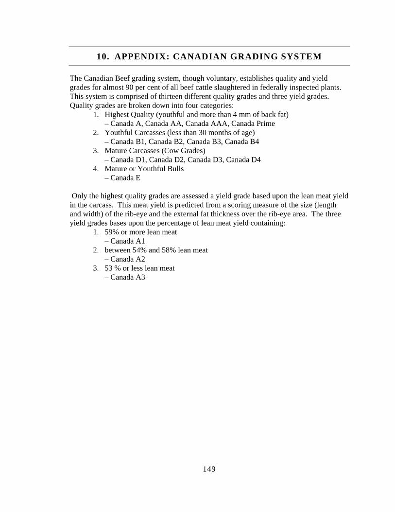
149

10. APPENDIX: CANADIAN GRADING SYSTEM

The Canadian Beef grading system, though voluntary, establishes quality and yield grades for almost 90 per cent of all beef cattle slaughtered in federally inspected plants. This system is comprised of thirteen different quality grades and three yield grades. Quality grades are broken down into four categories:

1. Highest Quality (youthful and more than 4 mm of back fat) – Canada A, Canada AA, Canada AAA, Canada Prime

2. Youthful Carcasses (less than 30 months of age) – Canada B1, Canada B2, Canada B3, Canada B4

3. Mature Carcasses (Cow Grades) – Canada D1, Canada D2, Canada D3, Canada D4

4. Mature or Youthful Bulls – Canada E

Only the highest quality grades are assessed a yield grade based upon the lean meat yield in the carcass. This meat yield is predicted from a scoring measure of the size (length and width) of the rib-eye and the external fat thickness over the rib-eye area. The three yield grades bases upon the percentage of lean meat yield containing:

1. 59% or more lean meat – Canada A1

2. between 54% and 58% lean meat – Canada A2

3. 53 % or less lean meat – Canada A3