Embed Size (px)
Citation preview

i
Project Report 2:14
A Profile of the Energy Sector in Tennessee
A Report to the Tennessee State General Assembly
i
Project Report 2:14
A Profile of the Energy Sector in Tennessee
ByMatthew N. Murray, Director
Howard H. Baker Jr. Center for Public Policy
Charles Sims, Baker Faculty FellowBruce Tonn, Baker FellowJean Peretz, Baker Fellow
Howard H. Baker Jr. Center for Public Policy
Jeff Wallace, Ryan Hansen, and Lew AlvaradoSparks Bureau of Business and Economic Research
University of Memphis
December 15, 2014
i
Project Report 2:14
A Report to the Tennessee State General Assembly
ByMatthew N. Murray, Director
Howard H. Baker Jr. Center for Public Policy
Charles Sims, Baker Faculty FellowBruce Tonn, Baker FellowJean Peretz, Baker Fellow
Howard H. Baker Jr. Center for Public Policy
Jeff Wallace, Ryan Hansen, and Lew AlvaradoSparks Bureau of Business and Economic Research
University of Memphis
December 15, 2014
i
A Profile of the Energy Sector in Tennessee
A Report to the Tennessee State General Assembly
ByMatthew N. Murray, Director
Howard H. Baker Jr. Center for Public Policy
Charles Sims, Baker Faculty FellowBruce Tonn, Baker FellowJean Peretz, Baker Fellow
Howard H. Baker Jr. Center for Public Policy
Jeff Wallace, Ryan Hansen, and Lew AlvaradoSparks Bureau of Business and Economic Research
University of Memphis
December 15, 2014
Baker Reports 4:15
How Do Motorists' Own Fuel Economy Estimates Compare with Official Government Ratings?
A Statistical Analysis
David L. Greene, PhDSenior Fellow, Energy & Environmental Policy Program
Howard H. Baker Jr. Center for Public Policy
Asad Khattak, PhD Jun Liu, PhD
Civil & Environmental Engineering
Janet L. Hopson, PhDEarth & Planetary Science
The University of Tennessee, Knoxville
Xin Wang, PhDVirginia Department of Transportation
Rick GoeltzOak Ridge National Laboratory
October 1, 2015

ii
Baker Center BoardCynthia BakerMedia ConsultantWashington, DC
Sam M. Browder Retired, Harriman Oil
Sarah Keeton Campbell Special Assistant to the Solicitor General and the Attorney General, State of TennesseeNashville, TN
Jimmy G. CheekChancellor, The University of Tennessee, Knoxville
AB Culvahouse Jr.Attorney, O’Melveny & Myers, LLP Washington, DC
The Honorable Albert Gore Jr. Former Vice President of the United States Former United States SenatorNashville, TN
Thomas GriscomCommunications ConsultantFormer Editor, Chattanooga Times Free Press Chattanooga, TN
James Haslam IIChairman and Founder, Pilot Corporation The University of Tennessee Board of Trustees
Joseph E. JohnsonFormer President, University of Tennessee
Fred MarcumFormer Senior Adviser to Senator Baker Huntsville, TN
The Honorable George Cranwell Montgomery Former Ambassador to the Sultanate of Oman
Regina Murray Knoxville, Tennessee
Lee RiedingerVice Cancellor, The University of Tennessee, Knoxville
Don C. Stansberry Jr.The University of Tennessee Board of Trustees Huntsville, TN
The Honorable Don Sundquist Former Governor of Tennessee Townsend, TN
The Honorable Fred Thompson Former United States Senator Washington, DC
Robert WallerFormer President and CEO, Mayo ClinicMemphis, TN
Baker Center Staff
Matt Murray, PhDDirector
Nissa Dahlin-Brown, EdDAssociate Director
Charles Sims, PhDFaculty Fellow
Kristia Wiegand, PhDFaculty Fellow
Jay CooleyBusiness Manager
William Park, PhDDirector of Undergraduate ProgramsProfessork, Agricultural and Resource Economics
About the Baker CenterThe Howard H. Baker Jr. Center for Public Policy is an education and research center that serves the University of Tennessee, Knoxville, and the public. The Baker Center is a nonpartisan institute devoted to education and public policy schol-arship focused on energy and the environment, global security, and leadership and governance.
Howard H. Baker Jr. Center for Public Policy1640 Cumberland Avenue Knoxville, TN 37996-3340
DisclaimerThis research was sponsored by the Oak Ridge National Laboratory. Findings and opinions conveyed herein are those of the author(s) only and do not necessarily represent an official position of the Howard H. Baker Jr., Center for Public Policy, the University of Tennessee, the US Department of Energy or Oak Ridge National Laboratory.
Patrick ButlerCEO, Assoc. Public Television StationsWashingtonk, DC
Elizabeth Woody Office Manager
Kristin EnglandInformation Specialist
Baker Center Board
Cynthia BakerMedia ConsultantWashington, DC
Sam M. BrowderRetired, Harriman Oil
Patrick ButlerCEO, Assoc. Public Television StationsWashington, DC
Sarah Keeton CampbellAttorney, Special Assistant to the Solicitor General and the Attorney General, State of TennesseeNashville, TN
Jimmy G. CheekChancellor, The University of Tennessee, Knoxville
AB Culvahouse Jr.Attorney, O’Melveny & Myers, LLPWashington, DC
The Honorable Albert Gore Jr.Former Vice President of The United StatesFormer United States SenatorNashville, TN
Thomas GriscomCommunications ConsultantFormer Editor, Chattanooga Times Free PressChattanooga, TN
James Haslam IIChairman and Founder, Pilot CorporationThe University of Tennessee Board of Trustees
Joseph E. JohnsonFormer President, University of Tennessee
Fred MarcumFormer Senior Advisor to Senator BakerHuntsville, TN
The Honorable George Cranwell MontgomeryFormer Ambassador to the Sultanate of Oman
Regina MurrayKnoxville, TN
Lee RiedingerVice Chancellor, The University of Tennessee, Knoxville
Don C. Stansberry Jr.The University of Tennessee Board of TrusteesHuntsville, TN
The Honorable Don SundquistFormer Governor of TennesseeTownsend, TN
The Honorable Fred ThompsonFormer United States SenatorWashington, DC
Robert WallerFormer President and CEO, Mayo ClinicMemphis, TN
Baker Center Staff
Matt Murray, PhDDirector
Nissa Dahlin-Brown, EdDAssociate Director
Charles Sims, PhDFaculty Fellow
Krista Wiegand, PhDFaculty Fellow
Jay CooleyBusiness Manager
Elizabeth WoodyOffice Manager
Kristin EnglandInformation Specialist
William Park, PhDDirector of Undergraduate ProgramsProfessor, Agricultural and Resource Economics
About the Baker CenterThe Howard H. Baker Jr. Center for Public Policy is an education and re-search center that serves the University of Tennessee, Knoxville, and the public. The Baker Center is a nonpartisan institute devoted to education and public policy scholarship focused on energy and the environment, global security, and leadership and governance.
Howard H. Baker Jr. Center for Public Policy1640 Cumberland AvenueKnoxville, TN 37996-3340
DisclaimerThis research was funded by Oak Ridge National Laboratory (ORNL) and carried out by researchers at ORNL and the University of Tennessee’s Howard H. Baker, Jr. Center for Public Policy and Department of Civil and Environmental Engineering. The views expressed herein are those of the authors alone and do not necessarily represent the views of Oak Ridge National Laboratory, UT-Battelle or the U.S. Department of Energy.

The Howard H. Baker Jr. Center for Public Policy3
TABLE OF CONTENTS
Abstract ...................................................................................................... 4
Acknowledgements .................................................................................... 4
I. Introduction ........................................................................................ 5
II. Previous Research .............................................................................. 8
III. Data .................................................................................................. 12
IV. Method ............................................................................................. 17
V. Results .............................................................................................. 19
V. Conclusions ...................................................................................... 30
VI. References ........................................................................................ 33
Appendix: ............................................................................................... 36

The Howard H. Baker Jr. Center for Public Policy4
AbstractUS government fuel economy tests are used for two primary purposes: 1) to monitor
automobile manufacturers’ compliance with fuel economy and greenhouse gas emissions standards and 2) to inform consumers about the fuel economy of passenger cars and light trucks. This study analyzes a unique database of 75,000 fuel economy estimates self-reported by customers of the US government website www.fueleconomy.gov to evaluate the effectiveness of the government’s estimates for these two purposes. The analysis shows great variability in individuals’ own fuel economy estimates relative to the official government estimates, but much smaller bias relative to the sample average. For consumers, the primary limitation of government fuel economy estimates is their uncertainty for a given individual rather than bias relative to the average individual. The analysis also examines correlations between individuals’ fuel economy estimates and specific technologies, vehicle class, driving style, method used to calculate fuel economy, manufacturer, and state. There is some evidence that the shortfall between test cycle fuel economy estimates (used to measure compliance with regulations) and in-use fuel economy estimates (such as those provided by customers of www.fueleconomy.gov) has been increasing since 2005. The direction and magnitude of the trend is consistent with changes made by the Environmental Protection Agencies to its methods for calculating the benefits of the standards in the 2010 and 2012 rulemakings. However, if the trend continues, it could affect the benefits realized by fuel economy and greenhouse gas emissions standards. A scientifically designed survey of in-use fuel economy is needed to insure that an unbiased sample is collected and that fuel economy is rigorously and consistently measured for all vehicles. The potential for information technology to reduce the uncertainty in predicting individuals’ on-road fuel economy should be explored.
AcknowledgementsThis research was funded by Oak Ridge National Laboratory (ORNL) and carried out by
researchers at ORNL and the University of Tennessee’s Howard H. Baker, Jr. Center for Public Policy and Department of Civil and Environmental Engineering. The views expressed herein are those of the authors alone and do not necessarily represent the views of Oak Ridge National Laboratory, UT-Battelle or the US Department of Energy.

The Howard H. Baker Jr. Center for Public Policy The Howard H. Baker Jr. Center for Public Policy5
How do Motorists’ Own Fuel Economy Estimates Compare with Official Government Ratings? A Statistical Analysis
David L. GreeneAsad Khattak
Jun LiuJanet L. Hopson
The University of Tennessee, Knoxville
Xin WangVirginia Department of Transportation
Rick GoeltzOak Ridge National Laboratory
October 1, 2015
I. IntroductionThe window sticker of every new passenger car or light truck sold in the US bears a label
with a prominently displayed government fuel economy rating. The intent is to provide consumers with consistent and reliable information they can use when comparing vehicles. Each label also contains the following caveat: “Actual results will vary for many reasons, including driving conditions and how you drive and maintain your vehicle.” Differences between consumers’ experiences with fuel economy and label values have been a source of discussion and dissatisfaction with the official government ratings since shortly after they were first introduced in 1975 (McNutt et al., 1978).
The US Environmental Protection Agency (EPA) provides two sets of fuel economy estimates (“test cycle” and “label”) for every make, model, engine and transmission configuration of passenger car and light truck sold in the US1 These estimates are important for two main reasons: (1) to enforce the Corporate Average Fuel Economy (CAFE) and greenhouse gas (GHG) emissions regulations for light-duty vehicles (EPA, 2012) the government needs test cycle estimates that are equitable to manufacturers, repeatable and proportional to real world experience and (2) consumers need accurate fuel economy estimates to make informed choices when buying vehicles.
1 In fact, most vehicle testing is done by the vehicle manufacturers, who certify to the EPA that the tests have been done in accordance with government procedures. The EPA tests 15-20% of vehicles each year to verify compliance (EPA, 2014a).

The Howard H. Baker Jr. Center for Public Policy6
In statistics, the terms accurate, precise and unbiased have specific, mathematical definitions. Accuracy measures the closeness of agreement between repeated measures of a given quantity and its true value. Precision measures the closeness of agreement between repeated measures of a given quantity and the mean of those measures. Bias measures the difference between the mean of a series of measurements or predictions and the true value of a quantity or the true mean of a population. The situation is somewhat different for government fuel economy estimates. A single number (e.g., a car’s fuel economy label number) is proposed as a useful estimate of the actual fuel economies of all motorists using the same vehicle2. In this case, there is no “true value” but rather a distribution of values for individual drivers. Assuming that the government fuel economy estimate is intended to correspond to the average fuel economy of all drivers of a given vehicle, bias can be defined as the difference between the official estimate and the mean of the population.3 Because there are not repeated measurements for an actual or even hypothetical true value of fuel economy, how to define accuracy and precision is less clear.4 In this paper we will quantitatively describe the deviations of individual motorists’ estimates from their vehicle’s fuel economy rating as variance. At the same time, we recognize that from an individual motorist’s perspective, the official rating might be perceived as biased or inaccurate.
The government is well aware of the issue of the variance of individual fuel economy results. Every fuel economy label contains the following caveat:
“Actual results will vary for many reasons, including driving conditions and how you drive and maintain your vehicle.”
It is quite possible for fuel economy ratings to be unbiased (reasonably predict the average fuel economy of all motorists) but poor predictors of the experiences of individuals. For the purposes of testing compliance with fuel economy standards, unbiased fuel economy estimates would be sufficient. If the expected fuel economy improvements are realized on average, the expected benefits in petroleum and greenhouse gas (GHG) reductions will be achieved. In fact, all that is necessary for the expected benefits to be realized is that a given percent increase in miles per gallon (MPG) on the test cycle produce the same percentage increase in on-road fuel economy. On the other hand, for the fuel economy label estimates to be of greatest value to consumers’ car purchase decisions, they should accurately predict the fuel economy an individual will experience on the road. This is clearly not achievable with a single-number rating for each vehicle. However, modern information technology might possibly enable relatively accurate prediction of individuals’ fuel economy.
2 Here, a vehicle means a unique vehicle as defined for regulatory purposes, typically a specific configuration of make, model, model year, engine and transmission.3 When fuel economy is measured in miles per gallon, the simple average of the fuel economies of a population of drivers will not equal the sum of all miles driven divided by the sum of all gallons consumed. The harmonic mean of the individual fuel economies, weighted by each vehicle’s miles traveled will.4 A single estimate for a range of values is absolutely precise because its variance is zero. On the other hand, it is inherently inaccurate; the only question being how inaccurate it is.

The Howard H. Baker Jr. Center for Public Policy The Howard H. Baker Jr. Center for Public Policy7
The test cycle fuel economy estimates used to determine manufacturers’ compliance with regulations are based on laboratory testing of vehicles over two (city and highway) driving cycles as required by statute. These drive cycles have been in use since the Corporate Average Fuel Economy (CAFE) standards were enacted in 1975. The label fuel economy estimates provided on the window stickers of new vehicles and used in advertising and the media are based on five drive cycles, adjusted in an attempt to reflect average US on-road experience. The five cycles include the “city” and “highway” cycles used to determine compliance with fuel economy and greenhouse gas emission standards plus additional cycles that reflect, 1) more aggressive driving behavior, 2) the impact of operating under colder ambient conditions and, 3) the impact of air conditioner use.
This study addresses how well the test cycle and label estimates serve their intended purposes though a statistical analysis of approximately 75,000 individual fuel economy estimates voluntarily submitted to the “My MPG” section of the government website www.fueleconomy.gov. The relationship between individuals’ own fuel economy estimates (My MPG) and the EPA label estimates is analyzed to determine whether the adjusted EPA estimates are unbiased and to measure the variability of consumers’ experiences relative to the label numbers. The relationship between individuals’ My MPG estimates and EPA test cycle estimates is examined to shed light on whether the ratio of test cycle to on-road MPG has been changing with succeeding model years. A continually increasing gap would imply that the government’s fuel economy standards might not achieve as much reduction in oil use and GHG emissions as intended.5 The need to monitor on-road fuel economy was recognized by the Environmental Protection Agency (EPA) and the National Highway Traffic Safety Administration (NHTSA) in their fuel economy and greenhouse gas rule for light-duty vehicles.
“The agencies recognize the potential for future changes in driver behavior or vehicle technology to change the on-road gap to be either larger or smaller.” (Federal Register, 2012, p. 62715)
The agencies assumed that a gap of 20%, which is consistent with fuel economy labeling, would continue through 2025, with minor adjustments for fuel energy content (EPA, 2012, pp. 4-1 to 4-7). This represents an increase of 5% over the 15% gap that had been assumed in previous EPA analyses.
The impacts of fuel efficient technologies such as turbo-charging and transmissions with higher gear counts are estimated to see if they perform better or worse on the road in comparison to the test cycles. The analysis also attempts to take into account driving conditions that vary from state to state and other factors that might influence on-road fuel economy.
5 The agencies’ rulemaking assumes the gap will remain at 20% through 2025, with some minor adjustments for fuel energy content and air conditioner efficiencies (EPA, 2012, pp. 4-2 to 4-7).
The Howard H. Baker Jr. Center for Public Policy8
The scope of this study is limited to light-duty vehicles with conventional gasoline (gasoline), gasoline-electric hybrid (hybrid), and diesel powertrains due to the nature of the data available from www.fueleconomy.gov .
II. Previous Research
When the EPA fuel economy estimates were first introduced in 1975, they were not adjusted for real-world driving conditions. Concern about the ability of the test cycle estimates to measure on-road fuel economy motivated assessments by government, industry and consumer groups. In the first year the CAFE Standards took effect (1978), researchers at the US Department of Energy (DOE) published an analysis of over 5,000 fuel economy records for model year 1974 to 1977 vehicles, obtained from a variety of sources (McNutt et al., 1978). Noting that the test cycle estimates were “fairly representative” of the on-road values for the 1974 model year, the researchers observed a trend of increasing shortfall.
“However, beginning in the 1975 model year and continuing through 1977 (the limits of existing data) the EPA certification values become an increasingly poorer representation of actual on-road fuel economy.”
They estimated that the average shortfall had increased from 4% in model year 1974 to about 20% for model year 1977.
In 1980 and 1981, General Motors (GM) conducted surveys of private owners of 1981 model year vehicles and asked them to record odometer readings and fuel purchases at their next four fill-ups (Schneider et al., 1982). From the 38,466 forms mailed out in the 1981 survey, 4,923 (12.8%) usable responses were received. The EPA test cycle combined fuel economy estimate for the vehicles was 25.5 miles per gallon (MPG) while the respondents’ average on-road fuel economy was 22.0 MPG, implying a shortfall of almost 14%. The earlier 1980 survey had produced an estimated shortfall of just over 16%. Front-wheel drive vehicles averaged a 6.4% smaller shortfall than rear-wheel drive vehicles, diesels had a 6.5% smaller shortfall than gasoline vehicles, and manual transmissions had 7.2% higher on-road fuel economy than automatic transmissions.
A study by Ford based on data from employees who leased Ford vehicles found that the shortfall for 1978 model year vehicles averaged 20%, but for 1979 and later model year vehicles, the shortfall was relatively stable at about 14% (McKenna and South, 1982). The Ford study also found that the shortfall for winter driving was 10% greater than for summer driving.
Analyzing a much larger data base of 56,395 vehicles amassed from a variety of sources, McNutt et al. (1982) found large variations in the fuel economy shortfall by model year but no consistent trend over time. They also found important differences between passenger cars and light trucks, rear-wheel drive and front-wheel drive vehicles, and manual and automatic transmissions. Their data showed a strong tendency for the percent shortfall to increase with

The Howard H. Baker Jr. Center for Public Policy The Howard H. Baker Jr. Center for Public Policy9
increasing fuel economy. Overall, they estimated a shortfall of 21% for model year 1981 vehicles. Having quantified variations in the shortfall by technology, vehicle class, model year and make and model, the study was the first to analyze the implications of uncertainties about on-road fuel economy for car buyers:
“These impacts include the inability of new car buyers to accurately compare different model vehicles and the difficulty in projecting future fuel demand based on the EPA val-ues.”
These studies and other evidence led the US EPA to adjust downward the fuel economy estimates reported to the public on window stickers and in advertising (Hellman and Murrell, 1984). A vehicle’s fuel economy estimate on the city test cycle was multiplied by 0.90 and its highway cycle estimate was multiplied by 0.78. The effect on a typical vehicles combined6 fuel economy estimate was approximately a 15% reduction relative to the test cycle numbers. However, the unadjusted test cycle numbers continued to be used to determine compliance with fuel economy standards, as required by statute, and they still are today.
At least one subsequent analysis of on-road fuel economy suggested that the on-road shortfall might have increased since the 1984 study. Mintz et al. (1993) analyzed data from the Energy Information Administration’s (EIA) 1985 Residential Transportation Energy Consumption Surveys (RTECS). RTECS collected gasoline purchase and odometer reading diaries from 3,891 households representing 8,401 vehicles. Comparing the on-road estimates to the unadjusted EPA test cycle MPG values, they found a shortfall of 18.7% for passenger cars and 20.1% for light trucks, somewhat larger than Hellman and Murrell’s (1984) 15%.
Despite the adjustments to EPA label estimates, the “shortfall” or “gap” between the EPA label estimates of new car fuel economy and what real people achieve in their day-to-day driving continued to be a topic of interest to the public and the media (e.g., O’Dell, 2012). Some media organizations conduct their own tests on public roads in order to compare “real-world” estimates to the EPA’s label estimates. Consumer Reports, for example, has made such comparisons for years. In a 2005 study, it concluded that fuel economy for conventional gasoline vehicles averaged 9% worse than label estimates, while hybrids were 18% below the label estimates (ConsumerReports.org, 2013). In 2008, the EPA (2006a) made further downward adjustments to label estimates. Consequently, a 2013 Consumer Reports study found conventional gasoline vehicles averaged only 2% below the EPA label estimates while hybrids fell short by 10%.
In developing the new 2008 fuel economy label estimates, the EPA analyzed several sources of on-road fuel economy estimates (EPA, 2013, Ch. 2). One was a sample of 8,180 estimates for 4,092 vehicles from users of the My MPG section of the DOE/EPA website www.fueleconomy.gov. For conventional gasoline vehicles, the My MPG data indicated that the label numbers
6 The combined fuel economy estimate is a weighted harmonic mean of the city and highway estimates, equal to 1/((0.55/city)+(0.45/highway)). The adjusted formula is 1/((0.55/(0.90*city))+(0.45/(0.78*highway))).

The Howard H. Baker Jr. Center for Public Policy10
based on the 1984 adjustment procedures were still reasonable estimates of average on-road fuel economy. For conventional gasoline vehicles the average label to on-road shortfall was only 1.4%. However, the shortfall for hybrid vehicles averaged 8.2%. As discussed below, these results closely match those obtained by Greene et al. (2007) in an analysis of a similar sample of the My MPG data.
The EPA, the Coordinating Research Council (CRC), the Department of Transportation (DOT), and the DOE measured the fuel economy of 120 vehicles, including 30 hybrid vehicles, in the Kansas City region (EPA, 2006, Ch. 2). The vehicles were driven by their owners, and data were collected over a 24-hour period by means of portable emissions measurement systems. A zero-intercept regression line predicting on-road fuel economy as a function of the 1984 EPA fuel economy label estimate indicated that conventional gasoline vehicles would average about 0.6% higher fuel economy on the road than the label values suggested. For hybrids, however, an average shortfall of 11% was observed.
The problem of achieving a consistent, proportional relationship between fuel economy as measured on laboratory tests relative to what drivers will experience in the real world is not limited to the US Similar shortfalls between test cycle and on-road fuel economy have also been observed in China and much larger shortfalls have been reported for the EU. Two recent studies by the International Council on Clean Transportation (ICCT) found that the on-road to certification test shortfall for vehicles sold in the European Union (EU) has been increasing rapidly (Mock et al., 2014; Mock et al., 2013).
“All data sets we examined demonstrate the same over-arching trend: the discrepancy be-tween type-approval and real-world CO2 emissions is increasing. While in 2001 this gap was just 8 percent, it grew to 18 percent by 2008 and then to 38 percent in 2013.” (Mock et al., 2014, p. 43)
The ICCT analyses conclude that the increasing gap is most likely due to increasing use of technologies that perform better on the certification (“type approval”) test than in the real world, increasing use of flexibilities in the testing procedures, and external factors not accounted for in the test, such as increased use of air conditioning. On the other hand, increased use of strategies to maximize test results are cited by Dings (2013) as the most important factor. Dings attributes approximately half of the gap to permitted techniques for optimizing performance on the EU’s test procedures that do not correspond to benefits in actual use. He allocates the remaining 50% equally among factors omitted from the test (e.g., air conditioner use), differences between the test cycle and actual driving behavior and conditions, and unknown factors.
Like the data used in this study, the ICCT data came from self-selected samples or business fleets. Potential sources of bias are acknowledged and briefly discussed in the report. However, the ICCT studies assert that model-year trends in the on-road shortfall should be insensitive to the sample design provided that the design does not change across model years. Because of this, the fact that their sample is self-selected should not affect inferences about the increasing on-road

The Howard H. Baker Jr. Center for Public Policy The Howard H. Baker Jr. Center for Public Policy11
shortfall. The ICCT report also points to the fact that the trends are relatively consistent across different data sources.
Also relying on self-reported data obtained from customers of a fuel economy website, Chinese researchers measured the shortfall between official Chinese government estimates and the reported on-road fuel consumption (Huo et al., 2011). For 2009, they found that on-road fuel consumption (gallons per mile) averaged 15.5% above the test cycle numbers. For the 153 makes and models in their data base, the range of increased on-road fuel consumption was from -8% to +60%.
This study uses the My MPG data of www.fueleconomy.gov to analyze the relationships between both test cycle and label fuel economy and what motorists say they achieve in their real world driving. The My MPG data have been analyzed three times before but with fewer samples and model years than are included in this analysis. Greene et al. (2006) regressed reported My MPG numbers against the EPA label estimates using the first 3,221 estimates supplied by customers of www.fueleconomy.gov. The EPA label estimates were based on the 1984 adjustment method since the study predated the 2008 adjustment method. The study found that the adjusted label estimates were nearly unbiased predictors of the average fuel economy of My MPG customers. On the other hand, the EPA label estimates were highly imprecise predictors of any given customer’s MPG estimate. This led to the following conclusion.
“These results imply that what is needed is not less biased adjustment factors for the EPA estimates but rather more precise methods of predicting the fuel economy individual con-sumers will achieve in their own driving.” (p. 99)
Greene et al. (2006) also recomputed EPA label estimates for those customers who provided estimates of their percentages of city and highway driving. Using customer-specific city and highway MPG weightings reduced the mean standard error (MSE) of their model from 3.42 to 2.89, or by about 15%.
Lin and Greene (2011) analyzed 31,227 My MPG records using linear models and ordinary least squares (OLS) regression with robust error estimation. Their goal was to develop models that could more accurately predict a given individual’s on-road fuel economy using data that could readily be supplied by the motorist. They found that accuracy rather than bias remained the chief limitation of the EPA label estimates, and that the bias of the 2008 adjustment method, relative to the My MPG numbers, was greater than that of the 1984 method. Their best model, however, was able to reduce the mean squared error (MSE) of prediction by only about one third versus the “naïve” prediction that on-road fuel economy equals EPA label fuel economy.
The ICCT’s study of EU experience (Mock et al., 2013) includes a brief analysis of an earlier version of the My MPG data set used in this study. They concluded that the gap between US test

The Howard H. Baker Jr. Center for Public Policy12
estimates and the on-road data was relatively steady at about 20% until model year 2003. After 2003, they found that the gap increased, reaching about 35 percent for model year 2012.
III. Data
Data for this study were obtained from the joint DOE/EPA website www.fueleconomy.gov. Since 2005, the website’s My MPG section has offered its customers the opportunity to select their vehicles from its database, enter their own fuel economy estimates, compare their estimates with the official EPA label estimates, and share their estimates with other users of the website. The site accepts fuel economy estimates derived by any method, but it provides guidance on how to measure fuel economy and checks data entered for errors and plausibility (Goeltz et al., 2005). For those who want to create fuel purchase diaries, the site provides templates for entering odometer readings (or miles traveled), fuel quantities purchased, price paid, percentage of city and highway driving, and date for any number of refueling events. Consistency checks are made as data are entered, and potential errors are brought to the customer’s attention. Alternatively, customers may supply estimates based on their vehicles’ dashboard readout, their own calculations, or by simply guessing. 7 The distribution of vehicle records in the My MPG database by type of estimation method is shown in Table 1.
Table 1. Distribution of My MPG Data by Participant’s Method of Calculation
Method Frequency PercentVehicle’s Computer Display (dash) 11,804 15.3Miles & Fuel Purchase Diary (miles) 15,086 19.56Odometer & Fuel Purchase Diary (odom) 15,854 20.56Calculated by Own Method (math) 32,645 42.33Guess 779 1.01Other & Unknown 958 1.24Total 77,126
For estimates to be accepted, the customer must respond affirmatively to a return e-mail sent by the site, as a guard against spurious or repetitive entries. In order for customer-supplied estimates to be shown on fueleconomy.gov, they must pass validity tests. For this study, however, all e-mail validated data were accepted. Outlier detection was based on statistical criteria, as described below.
The My MPG data are susceptible to a variety of errors, including simple recording errors or calculation errors by those doing their own calculations. However, the website provides forms with built-in error checking for those entering odometer readings and fuel purchases at each fill
7 In 4,708 cases, estimates made by different methods were provided for the same vehicle. In the case of such repeated obser-vations, each estimate was treated as a distinct observation, resulting in 77,126 total observations for the 72,211 vehicles.
The Howard H. Baker Jr. Center for Public Policy The Howard H. Baker Jr. Center for Public Policy13
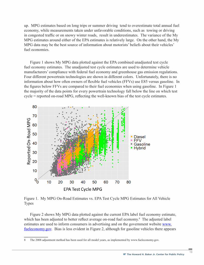
up. MPG estimates based on long trips or summer driving tend to overestimate total annual fuel economy, while measurements taken under unfavorable conditions, such as towing or driving in congested traffic or on snowy winter roads, result in underestimates. The variance of the My MPG estimates around either of the EPA estimates is relatively large. On the other hand, the My MPG data may be the best source of information about motorists’ beliefs about their vehicles’ fuel economies.
Figure 1 shows My MPG data plotted against the EPA combined unadjusted test cycle fuel economy estimates. The unadjusted test cycle estimates are used to determine vehicle manufacturers’ compliance with federal fuel economy and greenhouse gas emission regulations. Four different powertrain technologies are shown in different colors. Unfortunately, there is no information about how often owners of flexible fuel vehicles (FFVs) use E85 versus gasoline. In the figures below FFVs are compared to their fuel economies when using gasoline. In Figure 1 the majority of the data points for every powertrain technology fall below the line on which test cycle = reported on-road MPG, reflecting the well-known bias of the test cycle estimates.
Figure 1. My MPG On-Road Estimates vs. EPA Test Cycle MPG Estimates for All Vehicle Types
Figure 2 shows My MPG data plotted against the current EPA label fuel economy estimate, which has been adjusted to better reflect average on-road fuel economy.8 The adjusted label estimates are used to inform consumers in advertising and on the government website www.fueleconomy.gov. Bias is less evident in Figure 2, although for gasoline vehicles there appears
8 The 2008 adjustment method has been used for all model years, as implemented by www.fueleconomy.gov.

The Howard H. Baker Jr. Center for Public Policy14
to be a tendency for the label MPG to underestimate MPG at higher MPG values (most observations fall to the left of the line) and overestimate the reported on-road MPG at low MPG values (the majority of observations fall to the right of the line on which both values are equal and hence Label MPG > On-Road MPG). This tendency does not appear to apply to hybrid vehicles, however. Most estimates exceed the 2008 label MPG: 75% for gasoline vehicles, 93% for diesels and 60% for hybrids.
Figure 2. My MPG On-Road Estimates vs. EPA Label MPG Estimates for All Vehicle Types
The My MPG data have strengths and weaknesses. The large number of observations and detailed matches to the owners’ vehicles by make, model, engine and transmission make this a unique publicly available source of information. There are observations from every state and for every model year of vehicle from 1984 to 2015. The information supplied by many participants about method of estimation and driving style enables additional inferences. A disadvantage of the My MPG data is that participants are a self-selected sample. While the distribution of the sample can be compared with other known distributions, there remains a potential for bias related to the participants’ interest in fuel economy. The methods by which the data are provided by customers of www.fueleconomy.gov have not changed over time so that if there is a bias in the data it is likely to remain consistent over time.
While it is not possible to definitively establish bias or lack thereof, frequency distributions of the respondents give some indication of the representativeness of the sample. The distribution of respondents by type of vehicle is compared with model year sales by vehicle class from 2000

The Howard H. Baker Jr. Center for Public Policy The Howard H. Baker Jr. Center for Public Policy15
to 2014 (EPA, 2014b) in Table 2. Passenger cars appear to be over-represented in the My MPG sample and all types of light trucks somewhat under-represented. Table 2. Distribution of Vehicles by Vehicle Class for 2000-2014 Model Years
New vehicles as a share of production Shares in My MPG sample Mean Min Max
Car 52.7% 47.7% 60.5% Car 67.56%SUV 27.7% 18.9% 35.7% SUV 17.72%Pickup 13.4% 10.1% 16.1% Pickup 10.42%Minivan/Van 6.2% 3.8% 10.2% Minivan/Van 4.30%
The My MPG sample also appears to be reasonably geographically representative. A simple correlation of the sample frequencies by state with the 2010 Census state population estimates produced a correlation coefficient of 0.971. The correlation with the Federal Highway Administration’s state motor vehicle registration estimates for 2010 was similar, 0.976.9
One might suspect that individuals who would monitor their vehicles’ fuel economy and submit data to www.fueleconomy.gov would be more likely than the average driver to maximize fuel economy. Although the distribution of driving styles in the general population is not known, the distribution of participants by self-described driving style does not reveal a predominance of eco-drivers. Only 17% of the participants described themselves as more cautious than most drivers and only 2% said they drive to maximize fuel economy (Table 3). Nevertheless, the potential for bias in a self-selected sample remains. As a consequence, the results of this analysis must be interpreted with caution.
Table 3. Distribution of My MPG Participants by Self-Reported Driving Style
Driving Style of Primary Driver Count %1 to 5
% of Total
Drives for maximum gas mileage (1) 602 2.23 0.78Drives more cautiously than most (2) 4,709 17.43 6.11Drives with the flow (3) 7,024 25.99 9.11Drives a little faster than most (4) 9,709 35.93 12.59Accelerates quickly and passes whenever possible (5) 4,978 18.42 6.45Not reported 50,104 - 64.96Total 77,126
Three measures of fuel economy are used in the analysis below (Table 4). The corresponding distributions (including log-transformed distributions) are shown in Figure 3. The “My MPG” numbers are those reported by individuals throughout the US using www.fueleconomy.gov’s
9 Table MV-1, Highway Statistics 2010, accessed on 3/18/2015 at, http://www.fhwa.dot.gov/policyinformation/statistics/2010/mv1.cfm.

The Howard H. Baker Jr. Center for Public Policy16
My MPG system. MPG numbers adjusted by the EPA for use on vehicle window stickers and for public information are termed “EPA Label” estimates. “EPA Test Cycle” estimates are the unadjusted MPG estimates based on the EPA’s city and highway cycle dynamometer tests. The test cycle estimates are used to certify manufacturers’ compliance with fuel economy standards.
Table 4. Sample* Means of Three Fuel Economy Metrics
Fuel Economy Metric Sample Mean Std. Dev.My MPG User Estimate 26.02 10.02EPA Test Cycle Estimate 30.56 10.73EPA Label Estimate 23.08 7.35
*Includes only gasoline, hybrid and diesel powertrains. Outliers deleted if My MPG > 150 or <2, or if more than 5 standard errors above or below regression line of My MPG on EPA Label Estimate. 76,755 observations remained in the sample.
Other variables describe vehicle attributes or represent fixed model year or state effects. The variable “cid” stands for cubic inch displacement but is actually a vehicle’s engine size in cubic liters. Zero-one indicator variables include transmission type: “cvt” for continuously variable and “manual” for manual transmission. Transmissions with seven or more gears are designated by the variable “gears7”, six or more by “gears6.” Other indicator variables represent 4-wheel drive (fourwdr), all-wheel drive (allwdr), and front wheel drive (frontwdr). The categories of driving style are listed in Table 3, with the first five being represented by “style1” to “style5,” consecutively. The methods by which participants estimated their fuel economies are represented by the (1,0) variables ”dash,” “miles,” “odom” and “math,” as shown in Table 1. The ten largest auto manufacturers are represented by (1,0) variables with the rest combined being the default. Model years 1984 to 2014 and the 50 states plus the District of Columbia are also represented by fixed effects, with 2015 and state not reported used as the default values.

The Howard H. Baker Jr. Center for Public Policy The Howard H. Baker Jr. Center for Public Policy17
Figure 3 Distribution of My MPG, EPA Test Cycle and EPA Label estimates.
IV. MethodWhen estimating the relationships between MPG values measured on a dynamometer and
those measured on the road, there are three reasons for preferring the log-log functional form. The first is that it treats fuel economy (miles per gallon) and fuel consumption (gallons per mile) symmetrically (log(mpg) = -log(gpm)). Estimated coefficients would have identical values and standard errors but opposite signs. Each coefficient represents the percent change in fuel economy for a 1% change in the respective variable. The second reason is that the effects of many of the factors influencing vehicle fuel consumption are multiplicative rather than additive. For example, the efficiency with which the chemical energy in fuel is converted into mechanical work at a vehicle’s wheels is equal to the engine efficiency multiplied by the transmission efficiency, while the energy required to move a vehicle a given distance equals one over the drivetrain efficiency multiplied by the work that must be done to overcome aerodynamic drag, rolling resistance and inertia. The third reason, as will be shown below, is that the residuals from the log-log regression better approximate the more desirable properties of errors in regression models.
The general estimating equation is therefore,

The Howard H. Baker Jr. Center for Public Policy18
Equation 1
The coefficient β in the general equation represents the percent change in on-road MPG for a 1% change in test cycle MPG, controlling for the n variables xij. Alpha (α) is a common constant term, εi is a driver/vehicle-specific random error, and i is the index for each vehicle in the My MPG database. When the xij are (0,1) indicator variables, eb
j is the multiplicative effect of factor j on MPG. For example, if bj = -0.05, then eb
j = 0.951, implying that the effect of factor j is to reduce fuel economy by 4.9%.
The unconditional value of β is also of interest as a measure of the average US relationship between on-road and test cycle MPG.
Equation 2
Finally, the linear relationship between on-road MPG and the EPA estimates posted on new vehicles’ window stickers and used in advertising is also of interest because it describes the correlation between the information provided to consumers and what consumers experience. Larrick and Soll (2008) found that consumers interpret fuel economy information linearly in terms of miles per gallon rather than in terms of gallons per mile. A linear formulation is therefore used in this regression.
Equation 3
All the regressions in this report were carried out using the STATA® “regress” procedure, with the “robust” correction for heteroskedastic errors.10 Outliers for gasoline and diesel vehicles were identified by first regressing the log of observed MPG on the log of the combined test cycle fuel economy and a constant. The estimated variance of the residuals from the regression was used to detect potential outliers. Upper and lower bounds for outlier detection were increased in integer multiples of the MSE of regression until there was no evident truncation in the graphs of residuals. The mean squared error (MSE) of the regression is relatively large, reflecting the degree of variance evident in Figures 1 and 2. Because the residuals from the regression were skewed towards negative values, the upper boundary was set at +5 standard errors while the lower boundary was set at -6 standard errors from the combined adjusted EPA label MPG estimate. Errors are multiplicative in the logarithmic model, so a lower bound of -6*0.336 allows a fuel economy estimate 87% below the regression line while an upper bound
10 STATA® is a registered trademark of StataCorp LP (2015).

The Howard H. Baker Jr. Center for Public Policy The Howard H. Baker Jr. Center for Public Policy19
of +5*0.336 sets a limit of 5.4 times the regression line value. These outlier limits rejected only 302 observations (0.45%) from the gasoline vehicle sample. The MSE of the diesel regression is smaller but still large relative to predicted fuel economy. Only 13 hybrid records and five diesel records were deleted as outliers. The outlier detection regression results for gasoline and diesel vehicles are shown in Table 5.
Table 5. Outlier Detection Regressions of My MPG on EPA Test Cycle Combined MPG Esti-mates
Variable Estimate Standard Error
Significance Level
Root MSE
R-squared No. Obs.
Gasoline VehiclesTest MPG 0.9990 0.0053 0.000 0.3360 0.34 67,679Constant -0.1807 0.0178 0.000
Hybrid VehiclesTest MPG 0.8956 0.0155 0.000 0.2696 0.37 5,044Constant 0.0974 0.0608 0.109
Diesel VehiclesTest MPG 0.9327 0.0199 0.000 0.2012 0.51 2,267Constant 0.1516 0.0735 0.039
Analysis of the residuals from all the regressions reported below using the Stata™ hettest post-estimation tool indicated that they were heteroskedastic (p = 0.000) and skewed towards negative values. Therefore, all regressions reported below were estimated using the Stata™ variance covariance estimation procedure for robust errors.
V. Results
The simple regression model of equation (2) was estimated to determine the average relationship between test cycle and on-road MPG for all model years of gasoline, hybrid and diesel vehicles in the sample. Model year indicator variables were then added to the gasoline vehicle regression to explore the possibility of trends in the relationship over time. Next equation (3) was estimated for each of the three types of powertrains to measure the relationship between the information provided to consumers and their own fuel economy estimates. Finally, the more general equation (1) was estimated separately for each powertrain types and then again for only those gasoline vehicles with odometer based estimates.
Test Cycle and On-Road MPG Estimates
Relationships between the logarithms of reported on-road MPG and the EPA test cycle MPG without controlling for other variables were estimated to describe the average “shortfall” for all model years and vehicles implied by the My MPG estimates. Results are summarized in Table

The Howard H. Baker Jr. Center for Public Policy20
6. Test Cycle MPG is significant at the 0.001 level, although the R2 values are only 0.56 to 0.68, indicating a large amount of unexplained variance.
Table 6. Log-Log Regression of My MPG Estimates on EPA Test Cycle MPG Estimates (select-ed variables reported)
Variable Estimate Standard Error
Significance Level
Root MSE
R-squared No. Obs.
Gasoline VehiclesTest Cycle MPG 0.9964 0.0034 0.000 0.214 0.56 67,377Constant -0.1566 0.0114 0.000
Hybrid VehiclesTest Cycle MPG 0.9252 0.0098 0.000 0.160 0.64 5,031Constant -0.0115 0.0393 0.799
Diesel VehiclesTest Cycle MPG 0.9511 0.0160 0.000 0.143 0.68 2,262Constant 0.0858 0.0605 0.156
The coefficient of Test Cycle MPG in the gasoline regression, 0.996, indicates that a 1% increase in fuel economy on the test cycle translated, on average, into almost exactly a 1% increase in fuel economy on the road. The shortfall is determined by both coefficients. For gasoline vehicles, the estimated shortfall from EPA test cycle estimates to My MPG on-road fuel economy estimates is approximately -15%. This is virtually identical to the approximately 15% reduction specified by the EPA’s 1984 adjustment procedure (Hellman and Murrell, 1984), but somewhat less than the 19% to 20% shortfalls found by Mintz et al. (1993). It is also less than the approximately 20% average adjustment stipulated by the 2008 rule (EPA, 2006).
The hybrid results imply a shortfall of about 22% at an EPA test cycle MPG of 25, increasing to 27% at an EPA test cycle MPG of 60. For diesels, the shortfall is only about 7% at an EPA test cycle MPG of 25 and grows to 10% for a vehicle with an EPA test cycle MPG of 50. Both hybrids and diesels have MSE smaller than the gasoline vehicles. Still, even for diesels, a 2*MSE band would be approximately -23% to +30% of the predicted value.
Shortfalls for each drivetrain technology are shown in Figure 4 as a function of EPA test cycle MPG. The estimates are based on the regression results shown in Table 6 and represent the average relationship between test cycle and on-road MPG over the 1984-2015 model years. No model year effects or other variables were included in the regression. The estimated shortfalls for diesel and hybrid vehicles grow with increasing MPG, but the estimated shortfall for gasoline vehicles remains nearly constant at about 15% as MPG increases. Mathematically, this conclusion follows from the fact that the estimated coefficient of the logarithm of gasoline test

The Howard H. Baker Jr. Center for Public Policy The Howard H. Baker Jr. Center for Public Policy21
cycle MPG is approximately 1.0 (0.9964). Early studies, in which carbureted gasoline engines predominated, indicated increasing shortfall with increasing MPG (e.g., McNutt et al., 1982).
Figure 4. Estimated Shortfall as a Percentage of EPA Test Cycle MPG.
The My MPG data for gasoline vehicles indicates that the shortfall between on-road fuel economy and EPA test cycle estimates may have increased in recent years. A simple model was estimated that regressed the logarithm of My MPG versus the logarithm of EPA test cycle MPG, including model years 1984 to 2014 as indicator (0,1) variables. No other explanatory variables are included. An F-test indicated that the addition of the indicator variables was statistically significant at the 0.0001 level. The shortfall, Δ, is estimated as the ratio of the on-road MPG predicted by the model to the average test cycle MPG for light-duty vehicles reported by the EPA (2015, table 9.1) in the respective model year, minus 1. The MPG predicted by the model is the test cycle MPG raised to the power 1.042 (the coefficient of the log of test cycle MPG), multiplied by eC+δ
y , where C is the estimated constant term of the regression and δy is the estimated model year coefficient. Because the coefficient of the log of test cycle MPG is greater than 1.0, the shortfall is gradually reduced as MPG increases. The regression coefficients and related statistics can be found in the appendix.
The estimated fuel economy shortfalls for conventional gasoline vehicles by model year are shown as percent differences from the test cycle MPG in Figure 5. Upper and lower bounds based on the 95% confidence intervals of the model year coefficients are also shown. The estimated additional shortfall is very close to 15% from 1987 to at least 2006 and perhaps 2009. In 2010 it dips close to 20%, declines to over 25% in 2013 and then rebounds to about 22% in 2014 and 2015. Although the shortfall appears to have increased abruptly in recent years it may be stabilizing close to the 20% shortfall used by the EPA and NHTSA to estimate future benefits of the fuel economy and GHG emissions standards. As noted above, studies carried out in the

The Howard H. Baker Jr. Center for Public Policy22
1970s and 1980s estimated that the shortfall increased from 1974 to 1977 and then stabilized in the vicinity of 15% to 20%. The US trend is much less extreme than comparable shortfall estimates for vehicles sold in the EU, described above (Mock et al., 2014).
Figure 5. Estimated Fuel Economy Shortfall for Model Years 1984 to 2015.
Almost forty years ago, an apparent increase in shortfall followed the oil price shocks and gasoline shortages of 1973-74 and the adoption of the first fuel economy regulations in 1975. Similarly, the price of gasoline increased from about $2/gallon in 2004 to $3/gallon in 2008 and, after remaining nearly constant since 1985, the CAFE standards for light trucks were increased in 2005 and those for passenger cars in 2011. The timing of the increase in shortfall suggests the possibility that as standards are tightened (or gasoline prices increase) manufacturers increasingly design vehicles to perform well on the test cycle (and achieve higher label MPG), in the process increasing the gap between test cycle and on-road fuel economy. Blending of ethanol with gasoline approximately tripled between 2005 and 2011, at which point most gasoline contained approximately 10% ethanol by volume (EIA, 2015). Because ethanol has only 2/3 of the energy content of gasoline, this could increase the on-road shortfall by about 2%. The fuel economy estimates of recent model year vehicles would be based on fuel with approximately 10% ethanol while those of older model years would be more likely to be based on fuel with a lower ethanol content. Whether increasing gasoline prices or increasing fuel economy standards or ethanol use, or something else, caused the on-road gap to increase is an important topic for further investigation. Even more important is whether the gap will remain stable in the future, so that an increase in test cycle fuel economy continues to provide an equivalent percentage increase in on-road fuel economy. The apparent trend should be closely watched to insure that the gap does not increase further. Light-duty vehicle fuel economy on the test cycle increased from 24.0 MPG in 2004 to 30.6 in 2014, about 28% (EPA, 2014b). If the shortfall increased by about 7 percentage points over the same period, about one fourth of the test cycle fuel economy gain over that period may have been offset by the increased shortfall. However, because the

The Howard H. Baker Jr. Center for Public Policy The Howard H. Baker Jr. Center for Public Policy23
rulemaking calculated the benefits of the standards assuming a 20% shortfall, the implication for the projected benefits is very small provided that the gap does not continue to grow.
Label and On-Road MPG Estimates
To estimate the potential bias and variance of individual estimates around the label numbers, linear regressions of the My MPG values on only the combined adjusted (2008) EPA label values and a constant were estimated. These regressions describe the correlation between the information provided to consumers and their reported on-road MPG (Table 7).
Table 7. Linear Regressions of My MPG Estimates on EPA Combined Adjusted Label MPG Estimates (selected variables reported)
Variable Estimate Standard Error
Significance Level
Root MSE R-squared No. Obs.
Gasoline VehiclesLabel MPG 1.1521 0.0042 0.000 5.097 0.56 67,377Constant -0.4568 0.0879 0.000
Hybrid VehiclesLabel MPG 1.0757 0.0128 0.000 6.607 0.60 5,031Constant -1.5189 0.4888 0.002
Diesel VehiclesLabel MPG 1.2519 0.0188 0.000 5.709 0.60 2,262Constant -0.5601 0.5787 0.333
In the gasoline vehicle regression, the coefficient of EPA label MPG implies that the on-road MPG of My MPG participants averages about 13% better than the EPA label rating at 20 MPG and increasing to 14% better at 50 MPG. The hybrid regression results imply a smaller bias, ranging from +2.5% at 30 MPG to +5% at 60 MPG. Because the constant term is not statistically significant, for practical purposes it would be reasonable for hybrid buyers to assume that average on-road MPG will equal the EPA label MPG. However, that is true only with respect to the national average MPG. An individual’s experience is likely to differ greatly from the national average, as indicated by the MSE of more than 6 MPG. Diesels average +22% above the label values at 20 MPG, increasing to 24% at 50 MPG.
The fact that the fuel economy achieved by individuals will differ from the label estimate has long been recognized. Indeed, a statement to that effect is printed on every fuel economy label. The My MPG data indicate that the differences are relatively large. For a conventional gasoline vehicle with a label fuel economy of 25 MPG, the regression results indicate that a confidence bound of +/- 2*(root mean squared error) is +/- 40% of the label value. If a 25 MPG vehicle travels 10,000 miles per year and gasoline costs $2.50/gallon, the consumer can be 95% certain that its fuel costs will be somewhere between $600 and $1,400. Uncertainty of this magnitude

The Howard H. Baker Jr. Center for Public Policy24
can seriously hinder a consumer’s ability to make informed choices about fuel economy (Greene, 2011; Greene et al., 2013).11
Factors Correlated with On-Road MPG
The following sections describe the results of an expanded regression analysis, including additional variables describing vehicle technologies and driver attributes, as shown in equation 1. As in equation 1, all the expanded models regress the My MPG estimates against the test cycle MPG estimates and other variables. Key results are highlighted in the following sections. Full listings of coefficient estimates and related model statistics for the regressions are provided in an appendix to the report.
Gasoline Internal Combustion Engine Vehicles
This section describes the results of the expanded regression on the subset of vehicles with conventional gasoline engines. Because test cycle fuel economy is one of the explanatory variables, the coefficients of the technology and driver variables do not measure their total impact on fuel economy but instead measure impacts on on-road fuel economy relative to the test cycle. A positive coefficient indicates that a technology increases on-road fuel economy relative to the typical on-road vs. test cycle relationship. A negative coefficient indicates on-road performance that is below average. For example, a technology that increased fuel economy by 5% on the test cycle but only 4% on the road would have a coefficient of about -0.01. The coefficient of -0.01 represents a 1 percentage point increase in the average shortfall, say from 15% to 16%.
When additional variables are included, the coefficient of test cycle fuel economy has a mean value of 0.74, with a 95% confidence interval of 0.72 to 0.76, indicating that a 1% increase in test cycle fuel economy corresponds to a 0.74% increase in on-road fuel economy, all else being equal. Other factors are not equal, however, and they have a substantial influence on on-road fuel economy. Vehicles with larger displacement engines do slightly worse on the road: a doubling of engine size reduces on-road performance by about 2.6% relative to the test cycle.12 Vehicles with continuously variable transmissions (CVT) appear to get about the same miles per gallon on the road relative to their test values as vehicles with conventional transmissions. Manual transmissions do about 6.9% better than automatics in real world driving. Turbocharged engines are estimated to add about 1.7% to the on-road shortfall in comparison to naturally aspirated engines. The shortfall for turbocharged pickups is about 6% larger, a result that is consistent with a recent study by AAA (2015) also based on the My MPG data. However there were a relatively small number (67) of turbocharged pickup trucks in the dataset. On the other
11 An important, unanswered question is whether car buyers assume a high degree of correlation among fuel economy esti-mates for cars they are considering buying. This may depend on whether deviations from label fuel economy ratings are strongly correlated for vehicles owned by the same household. This issue is not analyzed in this report. Further analysis of the odometer and miles data are planned and may shed some light on this question.12 All the results reported in this section have a level of statistical significance of 0.05 or better, except where noted otherwise. Detailed results may be found in the appendix.

The Howard H. Baker Jr. Center for Public Policy The Howard H. Baker Jr. Center for Public Policy25
hand, the 542 turbocharged SUVs in the dataset do not show a statistically significant increase in their on-road shortfall, suggesting that the pickup effect may be a result of differences in usage (e.g., towing and hauling). Vehicles with higher gear counts appear to have a somewhat reduced shortfall but this result has a significance level of only 0.094. Four-wheel drive performs about 1.8% worse on the road while front wheel drive does about 1.3% better. With the exception of manual transmissions, none of the technology impacts are greater than 3%, indicating that the test cycle results are not strongly biased relative to on-road performance by these technologies.
Driving style matters. The estimated coefficients are relative to the style of the majority of observations which do not include a description of driving style.13 If the observations without an indication of driving style have driving styles similar to those that do, the driving style coefficients can be interpreted as differences from the typical driver. Drivers who described themselves as driving “for maximum fuel economy” or “more cautiously than most,” reduced their on-road short-fall by about 12% in comparison to those who chose “accelerate quickly and pass whenever possible” and by 8-10% relative to the average driver. The benefit of the more cautious driving styles closely matches other estimates of what an average driver can achieve by “eco-driving” (Greene, 1986; Kurani et al., 2013; IEA, 2005; Kurani et al., 2005).
There are a few statistically significant effects associated with manufacturers, but they combine the unobserved effects of driver behavior and environment with the design and manufacture of the vehicles. In general, manufacturer effects are small. The estimated coefficients range from 2.7% to 5.1% decreases in on-road performance for Ford, Chrysler, Nissan and Hyundai vehicles to zero effects for GM, Honda, Toyota and Volkswagen, to 0.7% to 1.5% increases for BMW and Daimler. Again, it is not possible to attribute these effects to a vehicle’s design and manufacture since they include unknown effects of behavior and environment.
Vehicle class effects (measured relative to compact cars) tend to be larger, with light trucks having greater shortfalls than passenger cars. The coefficients of minivans, SUVs, pickups, vans, and special purpose vehicles imply increased shortfalls of 6.4% to 11.5%, in comparison to compact passenger cars. Once again, the estimated effects cannot distinguish effects due to the way the vehicles are used (e.g., towing, hauling or off-road operation) from how they are designed.
In the expanded regression model the only model year effects significant at the 0.5 level are associated with the oldest two model years (1985, 1986) and model year 2013. Nonetheless, an F-test indicated that the model year effects, taken as a whole, are statistically significant at the 0.0001 level. The estimated effects for the oldest vehicles may reflect differences in usage patterns (e.g., shorter trips) and mechanical performance due to the age of the vehicles as much as model year specific effects. In general, the data do not indicate a deterioration of on-road
13 The option to specify driving style was added in 2007 after the My MPG system had been in effect for several years. Thus, early participants did not have the opportunity to indicate their driving style.
The Howard H. Baker Jr. Center for Public Policy26
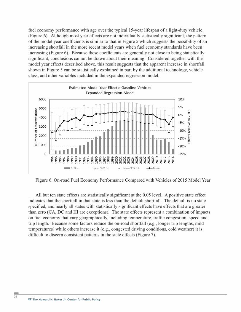
fuel economy performance with age over the typical 15-year lifespan of a light-duty vehicle (Figure 6). Although most year effects are not individually statistically significant, the pattern of the model year coefficients is similar to that in Figure 5 which suggests the possibility of an increasing shortfall in the more recent model years when fuel economy standards have been increasing (Figure 6). Because these coefficients are generally not close to being statistically significant, conclusions cannot be drawn about their meaning. Considered together with the model year effects described above, this result suggests that the apparent increase in shortfall shown in Figure 5 can be statistically explained in part by the additional technology, vehicle class, and other variables included in the expanded regression model.
Figure 6. On-road Fuel Economy Performance Compared with Vehicles of 2015 Model Year
All but ten state effects are statistically significant at the 0.05 level. A positive state effect indicates that the shortfall in that state is less than the default shortfall. The default is no state specified, and nearly all states with statistically significant effects have effects that are greater than zero (CA, DC and HI are exceptions). The state effects represent a combination of impacts on fuel economy that vary geographically, including temperature, traffic congestion, speed and trip length. Because some factors reduce the on-road shortfall (e.g., longer trip lengths, mild temperatures) while others increase it (e.g., congested driving conditions, cold weather) it is difficult to discern consistent patterns in the state effects (Figure 7).

The Howard H. Baker Jr. Center for Public Policy The Howard H. Baker Jr. Center for Public Policy27
Figure 7. Estimated State Effects: Gasoline Regression Model
The impact of method of estimation is interesting in part because, like the effect of driving style, it is indirectly related to the issue of self-selection bias. Differences among estimation methods could reveal tendencies for those reporting MPG numbers to “self-enhance” in order to appear achieve better than expected fuel economy. Four methods of estimation were represented in the model:
1. Dash: MPG estimate obtained from a vehicle’s dashboard display.2. Miles: MPG estimated by dividing miles between fill-ups by gallons purchased.
Participant supplies miles between fill-ups but not odometer readings.3. Odometer: MPG estimated by fueleconomy.gov by subtracting the odometer reading
at the current fill up from the reading at the previous fill up and dividing by gallons purchased at the current fill up. Most records consist of multiple fill ups and MPG is calculated as the sum of miles divided by the sum of gallons.
4. Math: MPG calculated by customer using own, unspecified method.
In the regression the default method is “did not answer”, “other” or “guess”. About 2.4% of the sample is in this category
Because of the error checking provided by www.fueleconomy.gov during the entry of odometer data, and because of the additional error checking performed for this study, the odometer and miles methods are believed to be the most reliable methods. In theory, the miles-based diary method should produce results similar to the odometer method, since both should be based on the same data: fuel purchases and miles traveled between fuel purchases. This seems to be the case. The estimated effects of the miles and odometer methods are close to each other, relative to the other methods. The “Odometer” method effect is statistically different from zero (at 2.1%), i.e., from the default category, although the “Miles” method effect is not. The effect

The Howard H. Baker Jr. Center for Public Policy28
of using a dashboard estimate is approximately 6.7% higher fuel economy than the default, while the “Math” method produces about 5.6% higher estimates.
Figure 8. Estimated Effects of Method of Calculating MPG
Even after taking all the above factors into account, the unexplained variance in the My MPG estimates for conventional gasoline vehicles is substantial. A two MSE confidence interval would be +49% to -33% of the predicted value. For a vehicle with a predicted fuel economy of 25 MPG, the two MSE interval would be 17 to 37 MPG.
Following the discussion of results for hybrids and diesels, we report estimates based only on the odometer sample of conventional gasoline vehicles (12,268 records) for comparison with the full sample. A more detailed analysis of the odometer and miles-based data is planned for future study.
Hybrids
The usable sample of hybrid vehicles for the expanded regression is much smaller, 4,807 records, but it includes all years in which hybrids were sold in the US from 1999 to 2015. The coefficient of test cycle MPG is smaller for hybrids than for gasoline vehicles: 0.67 vs. 0.74. The effect of (internal combustion) engine displacement is greater for hybrids: for every 10% increase in displacement fuel economy decreases by an average of 4.6%. The coefficient of CVT, is positive at 2.9%. The effect of a manual transmission is surprisingly large, a 13 percentage point reduction in the test cycle to on-road MPG shortfall; however, the early Honda Insights predominate in this group. Turbocharged hybrids are estimated to have a 20 percentage point greater shortfall but few hybrids are turbocharged. The effect of six or more gears is not significant. Four wheel or all-wheel drive vehicles have a 2.5 percentage point larger shortfall.

The Howard H. Baker Jr. Center for Public Policy The Howard H. Baker Jr. Center for Public Policy29
The effect of driving style is similar to that for gasoline vehicles. This may be surprising since many believe that hybrid vehicles are more sensitive to driving style than conventional gasoline vehicles. Like the drivers of conventional gasoline vehicles, those who drive “more cautiously than most” or “for maximum fuel economy” get 10% to 12% better fuel economy than those who “accelerate quickly and pass whenever possible”.
Relative to compacts (the default vehicle class), two-seater (mostly Honda Insights), do about 11% better on the road. SUVs are estimated to have about 9.7% larger shortfalls and large cars 7.4% larger shortfalls. Most manufacturer effects are not statistically significant. Most of the model year and state fixed effects are not statistically significant, in part reflecting the smaller sample size.
With respect to the methods of estimating MPG for hybrids, none of the method effects are statistically significantly different from zero.
Diesel
The diesel sample for the expanded regression is even smaller than the hybrid sample, totaling 2,116 usable records. As a consequence there are many fewer statistically significant variables. The coefficient of test cycle MPG is only 0.62, indicating that on-road fuel economy increases more slowly with test cycle fuel economy than for gasoline vehicles, other things being equal. Vehicles with manual transmissions have a smaller shortfall by 5.4 percentage points, but none of the other technology coefficient estimates are statistically significant. The effect of driving style on diesel fuel economy is smaller than that for gasoline vehicles with the most efficient two styles getting 6% to 7% better on-road fuel economy than the most inefficient. For diesels, the effect of the odometer method is also not significantly different from the miles method. Those basing their estimates on dashboard readouts report about 10% higher fuel economy relative to their test cycle numbers than those using the odometer method. Among vehicle classes, pickups and vans are estimated to have significantly greater shortfalls: -17% and -38%, respectively. Again, usage patterns are likely an important reason for the increased shortfall. Only one manufacturer effect is significant at the 0.05 level. None of the model year effects was statistically significant at the 0.01 level.
Odometer Sample for Gasoline Vehicles
The expanded model was re-estimated on the subsample of gasoline vehicles using the odometer record (12,268 usable records). The coefficient of test cycle MPG was slightly smaller 0.68 vs. 0.74. The estimated coefficients of most other technology variables were similar, although fewer were statistically significant. Four of the five driving style coefficient estimates were significant (relative to no answer). Again, the self-described fuel economy maximizing and more cautious groups did about 9% to 10% better than the most aggressive drivers. Most vehicle

The Howard H. Baker Jr. Center for Public Policy30
class effects were significant and, again, passenger cars had somewhat smaller shortfalls than light trucks.
The odometer data show a trend of increasing shortfall in model years that is very similar to the full gasoline vehicle sample (Figure 9). Like the full gasoline sample estimates, the effects are relative to 2015. In general, the individual model year effects are not statistically significant but the combination of all model year effects is statistically significant at the 0.003 level. Individually, only the effect for 1998 appears to be statistically significant. When compared with the statistically significant model year effects illustrated in Figure 5, this result and that for the full gasoline sample indicate that the variables included in the expanded regression model explain much of the increase in on-road shortfall since 2004 or 2005.
Figure 9. Estimated Fuel Economy Shortfall, Odometer Records: 1984-2014.
V. Conclusions
Perhaps the most important conclusion that can be confidently drawn from the My MPG data is that the variance of the fuel economy estimates reported by individuals is very large relative to the EPA MPG estimates for their vehicles. This conclusion is almost certainly valid whether the My MPG dataset is biased by self-selection or whether some individuals’ estimates are inflated by self-enhancing behavior. A very large fraction of the variation in individual estimates could not be accounted for by the vehicle and driver variables included in our full regression models. As Greene et al. (2007) and Lin and Greene (2011) observed, it appears that the EPA MPG estimates are not strongly biased in comparison to the

The Howard H. Baker Jr. Center for Public Policy The Howard H. Baker Jr. Center for Public Policy31
average fuel economy of all drivers, but that the estimates of individual drivers vary widely around the label estimates. This is to be expected given the variations in driving behavior, traffic conditions and other factors. Nonetheless, it reduces the value of fuel economy information in car buying decisions and could be an important explanation for why car buyers appear to undervalue fuel economy in car buying decisions (Sallee, 2013; Greene et al., 2013).
Modern information technology may offer a way to develop individualized fuel economy estimates. The information available from a modern vehicle’s computer control system could be combined with existing information technology to generate individualized driving cycles. Driving cycles for individual motorists could be used with vehicle simulation models, calibrated to individual vehicles, to develop personal fuel economy estimates for both new and used vehicles. While it is not clear how much estimation errors could be reduced, we believe this is an important area for future research that has the potential to enhance the value of fuel economy information to consumers.
The simple gasoline, hybrid, and diesel regression models indicate that, on average, a 1% increase in test cycle fuel economy has translated into very nearly a 1% improvement in on-road MPG. This is important because it indicates that relative improvements on the test cycle have produced equal relative improvements in on-road MPG. However, simple regressions including fixed effects for recent model years suggest that the test cycle vs. on-road gap has been growing in those years in which fuel economy standards have been increasing. Taken at face value, these results suggest that roughly one-fourth of the gain on the test cycle may have been offset by an increased gap. However, the impact on the fuel consumption and greenhouse gas reductions estimated for the standards is very small because the EPA rulemaking assumed the gap had increased from 15% to 20%. On the other hand, model year effects estimated using the expanded model, whether based on the full gasoline vehicle sample or just those using the odometer method, do not show such a large increase in the shortfall. This suggests that the technology, vehicle class and other variables included in the expanded model explain most of the increased shortfall. Given the limitations of the sample design, the evidence for an increasing gap in the US is not definitive and will have to be resolved by future research.
Driving style affects real-world fuel economy. Those who describe themselves as driving cautiously or attempting to maximize their fuel economy get about 10% more miles per gallon than average or aggressive drivers.
Turbo-charged engines appear to achieve slightly lower fuel economy in the real world than would be predicted based on their test cycle numbers. The same applies to 4-wheel drive vehicles and those with larger engines. The increases in the shortfall are small, however. In general, the on-road shortfalls for light trucks are greater than those for passenger cars. How much of this is due to how the vehicles are driven versus design and technological factors is not known.

The Howard H. Baker Jr. Center for Public Policy32
Although the data analyzed in this report are based on a self-selected sample, there are reasons to believe that the inferences drawn from it may be reliable. First, the distribution of vehicle types in the sample is generally similar to that of the vehicle fleet as a whole. Second, the vast majority of drivers do not describe themselves as driving to maximize fuel economy or even as driving more cautiously than most. Third, the statistical inferences based only on the data from drivers using the most rigorous odometer method are not generally different from those using other methods. Fourth, the estimates of the MPG shortfall, technology effects and driving style effects are generally consistent with the existing literature.
Nevertheless, the importance of fuel economy numbers for the enforcement of CAFE and GHG emissions standards and for informing car buyers’ decisions, together with the unresolved issues raised by this analysis, point to the need for further research. The authors plan to carry out a more detailed analysis of the odometer data to investigate how fuel economy varies over time, how errors relate to the length of the odometer diary record, and possible correlations among vehicles owned by the same household. Unfortunately, even this more detailed analysis will be limited by the sample design.
Ultimately, a new scientifically designed survey of in-use fuel economy is needed to insure that an unbiased sample is collected and that fuel economy is rigorously and consistently measured for all vehicles. In 2011 Transport Canada launched a Canadian Vehicle Use Study to measure the on-road fuel economy of Canadian vehicles by means of automated data loggers connected to each vehicle’s computer system (Transport Canada, 2015). With lessons learned from the Canadian experience, the US may be able to develop efficient and scientifically rigorous methods for measuring the relationship between test cycle fuel economy and consumers’ experience in real world driving.

The Howard H. Baker Jr. Center for Public Policy The Howard H. Baker Jr. Center for Public Policy33
VI. References1. AAA, 2015. “Test Results: Fuel Economy – Phase I & II”, Fact Sheet, accessed on 6/22/2015 at
http://publicaffairsresources.aaa.biz/wp-content/uploads/2015/06/FE2-Fact-Sheet-FINAL.pdf
2. Consumer Reports, 2013. “The mpg gap”, accessed on 1/26/2015 at http://www.consumerreports.org/cro/magazine/2013/08/the-mpg-gap/index.htm .
3. Energy Information Administration (EIA), 2015. “Fuel Ethanol Overview”, Annual Energy Review 2012, accessed on 8/26/2015 at http://www.eia.gov/totalenergy/data/annual/showtext.cfm?t=ptb1003 .
4. Goeltz, R., D.L. Greene, R.C. Gibson and J.L. Hopson, 2005. “Data Quality Assurance Procedures for User-Supplied Fuel Economy Data”, National Transportation Research Center, Oak Ridge National Laboratory, Oak Ridge, TN (available from R. Goeltz on request).
5. Greene, D.L., D.H. Evans and J. Hiestand, 2013. “Survey evidence on the willingness of US consumers to pay for automotive fuel economy”, Energy Policy, vol. 61, pp. 1539-1550.
6. Greene, D.L., 2011. “Uncertainty, Loss Aversion and Markets for Energy Efficiency”, Energy Economics, vol. 33, pp. 608-616.
7. Greene, D.L., J.L. Hopson, R. Goeltz and J. Li, 2007. “Analysis of In-Use Fuel Economy Shortfall Based on Voluntarily Reported Mile-per-Gallon Estimates,” Transportation Research Record, No. 1983, pp. 99-105.
8. Greene, D.L., 1986. Driver Energy Conservation Awareness Training: Review and Recommendations, ORNL/TM-9897, Oak Ridge National Laboratory, Oak Ridge, Tennessee, May 1986.
9. Hellman, K., and J.D. Murrell, 1984. “Development of Adjustment Factors for the EPA City and Highway MPG Values”, SAE Technical Paper Series 840496.
10. Huo, H., Z. Yao, K. He and X. Yu, 2011. “Fuel consumption rates of passenger, cars in China: Labels versus real-world”, Energy Policy, vol. 39, pp. 7130-7135.
11. International Energy Agency (IEA), Saving Oil in a Hurry, OECD, Paris.
12. Kurani, K., A. Sanguinetti and H. Park, 2015. “Actual Results May Vary: A Behavioral Review of Eco-Driving for Policy Makers”, White Paper, National Center for Sustainable Transportation, University of California at Davis, Davis, CA, July.
13. Kurani, K., T. Stillwater and M. Jones, 2013. Ecodrive I-80: A Large Sample Fuel Economy Feedback Field Test, Final Report, ITS-RR-13-15, Institute for Transportation Studies, Univ. of California, Davis, CA, available at https://www.fueleconomy.gov/feg/pdfs/EcoDrive%20I-80.pdf.
14. Larrick, R.P. and J.B. Soll, 2008. “The MPG Illusion”, Science, vol. 320, pp. 1593-1594, June.
15. Lin, Z. and D.L. Greene, 2011. Predicting Individual On-road Fuel Economy Using Simple Consumer and Vehicle Attributes, SAE Technical Paper Series No. 11SDP-0014, Society of Automotive Engineers, Warrendale, PA, April 12.

The Howard H. Baker Jr. Center for Public Policy34
16. McKenna, J.C. and N.E. South, 1982. “On-road Fuel Economy for 1978-1981 Ford Vehicles”, SAE Technical Paper Series 820789, Society of Automotive Engineers, Warrendale, PA.
17. McNutt, B.D., R. Dulla, R. Crawford and H.T. McAdams, 1982. “Comparison of EPA and On-Road Fuel Economy – Analysis Approaches, Trends and Imports”, SAE Technical Paper Series 820788, Society of Automotive Engineers, Warrendale, PA, June.
18. McNutt, B.D., D. Pirkey and R. Dulla, 1978. “A Comparison of Fuel Economy Results from EPA Tests and Actual In-Use Experience, 1974-1977 Model Year Cars”, SAE Paper 780037, Society of Automotive Engineers, Warrendale, PA.
19. Mintz, M.M., A.R.D. Vyas, and L.A. Conley, 1993. “Difference between EPA Test and In-Use Fuel Economy: Are the Correction Factors Correct?”, TRB Paper 931104, 72nd Annual Meeting of the Transportation Research Board, Washington, DC, January.
20. Mock, P., J. German, A. Bandivadekar, I. Riemersma, N. Ligterink and U. Lambrecht, 2014. From Laboratory to Road: A Comparison of Official and “Real-World” Fuel Consumption and CO2Values for Cars in Europe and the United States, White paper, International Council on Clean Transportation, Washington, D.C., available at http://www.theicct.org/laboratory-road.
21. Mock, P., U. Tiegete, V. Franco, J. German, A. Bandivadekar, N. Ligterink, U. Lambrecht, J. Kühlwein and I. Riemersma, 2014. From Laboratory to Road: A 2014 Update of Official and “Real-World” Fuel Economy and CO2Values for Passenger Cars in Europe, white Paper, International Council on Clean Transportation, San Francisco, September, available at http://theicct.org/laboratory-road-2014-update.
22. Posada, F. and J. German, 2013. “Measuring in-use fuel economy in Europe and the US: Summary of pilot studies”, Working Paper 2013-5, The International Council on Clean Transportation, http://www.theicct.org/sites/default/files/publications/ICCT_FuelEcon_pilotstudies_20131125.pdf , accessed on 2/6/2014.
23. O’Dell, J., 2012. “Here’s Why Real-World MPG Doesn’t Match EPA Ratings”, edmunds.com, posted 3/29/2012 and accessed on 1/26/2015 at http://www.edmunds.com/fuel-economy/heres-why-real-world-mpg-doesnt-match-epa-ratings.html .
24. Sallee, J.M. 2013. Rational Inattention and Energy Efficiency. Working Paper 19545, National Bureau of Economic Research, Cambridge, MA, October.
25. Schneider, R.W., W.S. Freas and T.P. McMahon, 1982. “In-Use Fuel Economy of 1981 Passenger Cars”, SAE Technical Paper Series 820790, Society of Automotive Engineers, Warrendale, PA.
26. StataCorp LP, 2015. Stata/SE 13.1 for Windows, Revision 03, June, 2015, College Station, TX.
27. Transport Canada, 2015. “Canadian Vehicle Use Study”, accessed at https://www.tc.gc.ca/eng/policy/aca-cvus-contact-2588.htm .
28. www.fueleconomy.gov, “Detailed Test Information: Detailed Comparison”, http://www.fueleconomy.gov/feg/fe_test_schedules.shtml , accessed on 3/16/2015.
29. US Department of Transportation, National Highway Traffic Safety Administration (NHTSA), 2012. Corporate Average Fuel Economy for MY 2017-MY 2025 Passenger Cars and Light Trucks, Final Regulatory Impact Analysis, Washington, D.C., August.

The Howard H. Baker Jr. Center for Public Policy The Howard H. Baker Jr. Center for Public Policy35
30. US Environmental Protection Agency (EPA), 2015. Light-Duty Automotive Technology, Carbon Dioxide Emissions, and Fuel Economy Trends: 1975 Through 2014, EPA-420-R -14-023a, Ann Arbor, MI, October 2014, “Full Report Tables”, accessed at http://www.epa.gov/otaq/fetrends-complete.htm on July 24, 2015.
31. US Environmental Protection Agency (EPA), 2014a. “Fuel Economy Testing and Labeling”, EPA-420-F-14-015, Ann Arbor, MI, April. Available at http://epa.gov/fueleconomy/documents/420f14015.pdf .
32. US Environmental Protection Agency (EPA), 2014b. Light-Duty Automotive Technology, Carbon Dioxide Emissions, and Fuel Economy Trends: 1975 Through 2014, EPA-420-R -14-023a, Ann Arbor, MI, October 2014.
33. US Environmental Protection Agency (EPA), 2012. “Joint Technical Support Document: Final Rulemaking for 2017-2025 Light-Duty Vehicle Greenhouse Gas Emission Standards and Corporate Average Fuel Economy Standards”, EPA-420-R-12-901, Ann Arbor, MI, August.
34. US Environmental Protection Agency (EPA), 2006a. “Fuel Economy Labeling of Motor Vehicles: Revisions to Improve Calculation of Fuel Economy Estimates”, Final Rule, Federal Register, vol. 71, no. 21, pp. 5425-5513, February 1.
35. US Environmental Protection Agency (EPA), 2006b. “EPA Issues New Test Methods for Fuel Economy Window Stickers”, EPA420-F-06-069, Office of Transportation and Air Quality, Ann Arbor, MI, http://www.epa.gov/otaq/carlabel/documents/420f06069.pdf.
36. US Environmental Protection Agency (EPA), 2006. Fuel Economy Labeling of Motor Vehicles: Revisions to Improve Calculations of Fuel Economy Estimates, Technical Support Document, EPA420-R-06-017, Office of Transportation and Air Quality, Ann Arbor, Michigan, December.

The Howard H. Baker Jr. Center for Public Policy36
Appendix:
Complete Models for Gasoline, Hybrid and Diesel Vehicles and Distributions for Dependent Variables

The Howard H. Baker Jr. Center for Public Policy The Howard H. Baker Jr. Center for Public Policy37
Gasoline Model Hybrid Model Diesel
Variable Estimate P-value Variable Estimate P-value Variable Estimate P-value
lucombined 0.744** 0.000 lucombined 0.667** 0.000 lucombined 0.623** 0.000
cid -0.026** 0.000 cid -0.046** 0.000 cid -0.023 0.281
cvt -0.004 0.374 cvt 0.029* 0.049 manual 0.054** 0.000
manual 0.069** 0.000 manual 0.130** 0.000 turbo -0.025 0.287
turbo -0.017** 0.000 turbo -0.200** 0.001 gears7 0.065 0.050
gears7 0.022 0.094 gear6 0.059** 0.009 fourwdr -0.092* 0.028
fourwdr -0.018** 0.000 fourwdr -0.025* 0.035 allwdr -0.110* 0.017
allwdr -0.012 0.092 dash 0.014 0.720 dash 0.018 0.562
frontwdr 0.013** 0.000 miles -0.001 0.983 miles -0.061* 0.040
dash 0.065** 0.000 odom -0.025 0.536 odom -0.084** 0.006
miles 0.000 0.975 math 0.011 0.793 math -0.032 0.278
odom 0.021** 0.005 style1 0.034* 0.026 style1 0.019 0.522
math 0.054** 0.000 style2 0.060** 0.000 style2 0.034** 0.006
style1 0.102** 0.000 style3 0.015* 0.014 style3 0.011 0.238
style2 0.083** 0.000 style4 -0.014* 0.022 style4 -0.027** 0.004
style3 0.029** 0.000 style5 -0.057** 0.000 style5 -0.036** 0.000
style4 -0.002 0.313 bmw 0.479** 0.000 bmw 0.014 0.861
style5 -0.033** 0.000 chrysler -0.048 0.851 chrysler -0.124 0.152
bmw 0.007 0.208 daimler 0.708** 0.000 daimler -0.060 0.477
chrysler -0.027** 0.000 ford 0.016 0.696 ford -0.038 0.723
daimler 0.015 0.066 gm -0.011 0.804 gm 0.027 0.745
ford -0.028** 0.000 honda 0.011 0.791 nissan 0.199** 0.001
gm -0.002 0.610 hyundai -0.037 0.419 toyota -0.008 0.936
honda 0.002 0.621 nissan -0.049 0.285 vw 0.048 0.528
hyundai -0.051** 0.000 toyota 0.021 0.610 class2 0.019 0.772
nissan -0.035** 0.000 vw 0.066 0.261 class3 0.032* 0.010
toyota 0.002 0.546 class2 -0.074** 0.000 class4 -0.173* 0.036
vw 0.002 0.684 class3 -0.018 0.099 class5 -0.009 0.848
class2 -0.001 0.777 class4 -0.017 0.855 class6 -0.044 0.660
class3 -0.009** 0.001 class5 -0.097** 0.000 class7 -0.009 0.490
class4 -0.091** 0.000 class6 0.111** 0.000 class8 -0.378** 0.000
class5 -0.084** 0.000 modelyear1 0.022 0.506 class9 -0.043** 0.000
class6 -0.064** 0.000 modelyear2 0.053 0.071 modelyear1 -0.081 0.461
class7 -0.068** 0.000 modelyear3 0.056* 0.047 modelyear2 0.033 0.560
class8 0.003 0.285 modelyear4 0.042 0.132 modelyear3 0.060 0.330
class9 0.033** 0.000 modelyear5 0.054 0.056 modelyear4 0.055 0.314
class10 -0.115** 0.000 modelyear6 0.066* 0.016 modelyear5 -0.002 0.978
class11 -0.017** 0.000 modelyear7 0.067* 0.018 modelyear6 -0.061 0.344
modelyear1 -0.118 0.087 modelyear8 0.039 0.165 modelyear7 -0.018 0.774
modelyear2 -0.113** 0.001 modelyear9 0.066* 0.024 modelyear8 0.045 0.387
modelyear3 -0.072* 0.029 modelyear10 0.058* 0.031 modelyear9 0.074 0.143
modelyear4 -0.038 0.241 modelyear11 0.024 0.377 modelyear10 0.149 0.202

The Howard H. Baker Jr. Center for Public Policy38
modelyear5 -0.042 0.178 modelyear12 0.024 0.384 modelyear11 -0.030 0.661
modelyear6 -0.027 0.390 modelyear13 0.016 0.560 modelyear12 0.028 0.680
modelyear7 -0.019 0.551 modelyear14 0.016 0.600 modelyear13 -0.005 0.930
modelyear8 -0.035 0.254 stdum1 -0.173** 0.002 modelyear14 -0.024 0.681
modelyear9 -0.001 0.986 stdum2 -0.013 0.648 modelyear15 0.011 0.820
modelyear10 -0.011 0.706 stdum3 0.037 0.393 modelyear16 -0.022 0.645
modelyear11 -0.010 0.747 stdum4 0.035 0.093 modelyear17 -0.023 0.602
modelyear12 0.007 0.814 stdum5 -0.029 0.132 modelyear18 0.007 0.873
modelyear13 0.006 0.846 stdum6 0.026 0.238 modelyear19 -0.002 0.960
modelyear14 0.008 0.798 stdum7 -0.011 0.636 modelyear20 0.016 0.725
modelyear15 0.013 0.663 stdum8 -0.003 0.936 modelyear21 0.004 0.929
modelyear16 0.017 0.579 stdum9 -0.012 0.756 modelyear22 0.023 0.612
modelyear17 0.015 0.613 stdum10 0.009 0.682 modelyear23 0.020 0.661
modelyear18 0.020 0.500 stdum11 0.014 0.549 modelyear24 -0.051 0.360
modelyear19 0.023 0.447 stdum12 -0.002 0.948 modelyear25 -0.058 0.329
modelyear20 0.017 0.576 stdum13 -0.005 0.873 modelyear26 -0.041 0.368
modelyear21 0.021 0.485 stdum14 0.066 0.288 modelyear27 -0.017 0.691
modelyear22 0.013 0.661 stdum15 0.015 0.482 modelyear28 -0.010 0.823
modelyear23 0.010 0.738 stdum16 0.028 0.246 modelyear29 -0.012 0.793
modelyear24 0.003 0.922 stdum17 -0.059* 0.036 modelyear30 0.004 0.928
modelyear25 0.003 0.932 stdum18 -0.004 0.869 modelyear31 0.003 0.947
modelyear26 0.004 0.900 stdum19 0.017 0.554 stdum1 0.057 0.117
modelyear27 -0.015 0.613 stdum20 0.028 0.227 stdum2 -0.012 0.768
modelyear28 -0.027 0.368 stdum21 0.023 0.294 stdum3 0.052 0.459
modelyear29 -0.029 0.324 stdum22 0.012 0.758 stdum4 0.018 0.568
modelyear30 -0.061* 0.039 stdum23 0.013 0.564 stdum5 0.027 0.317
modelyear31 -0.016 0.606 stdum24 -0.014 0.524 stdum6 0.034 0.235
stdum1 -0.015 0.363 stdum25 -0.019 0.459 stdum7 0.055 0.062
stdum2 0.044** 0.000 stdum26 -0.046 0.376 stdum8 -0.129** 0.005
stdum3 0.052** 0.000 stdum27 0.020 0.593 stdum9 0.018 0.621
stdum4 0.035** 0.000 stdum28 0.021 0.326 stdum10 0.015 0.593
stdum5 -0.018** 0.006 stdum29 -0.061 0.376 stdum11 0.037 0.177
stdum6 0.069** 0.000 stdum30 -0.029 0.344 stdum12 -0.013 0.876
stdum7 0.007 0.402 stdum31 0.035 0.180 stdum13 0.071* 0.023
stdum8 -0.094* 0.010 stdum32 -0.011 0.638 stdum14 0.018 0.722
stdum9 0.037** 0.003 stdum33 0.038 0.144 stdum15 0.052 0.065
stdum10 -0.003 0.664 stdum34 -0.010 0.670 stdum16 0.040 0.252
stdum11 0.017* 0.025 stdum35 -0.017 0.425 stdum17 0.051 0.181
stdum12 -0.065** 0.000 stdum36 0.025 0.243 stdum18 0.019 0.483
stdum13 0.036** 0.000 stdum37 0.001 0.973 stdum19 0.027 0.534
stdum14 0.047** 0.001 stdum38 -0.039 0.189 stdum20 0.062* 0.032
stdum15 0.015* 0.043 stdum39 -0.015 0.525 stdum21 0.116** 0.000
stdum16 0.032** 0.000 stdum40 -0.002 0.966 stdum22 0.109** 0.007
stdum17 0.041** 0.000 stdum41 -0.015 0.681 stdum23 0.044 0.127

The Howard H. Baker Jr. Center for Public Policy The Howard H. Baker Jr. Center for Public Policy39
stdum18 0.032** 0.003 stdum42 -0.037 0.120 stdum24 0.068* 0.016
stdum19 -0.002 0.844 stdum43 0.052 0.020 stdum25 0.049 0.087
stdum20 0.024 0.005 stdum44 -0.016 0.436 stdum26 0.066 0.017
stdum21 0.032 0.000 stdum45 0.011 0.643 stdum27 0.075 0.315
stdum22 0.088 0.000 stdum46 -0.006 0.763 stdum28 0.065 0.020
stdum23 0.056 0.000 stdum47 0.009 0.743 stdum29 0.115 0.085
stdum24 0.054 0.000 stdum48 -0.017 0.412 stdum30 0.091 0.004
stdum25 0.045 0.000 stdum49 0.016 0.477 stdum31 0.154 0.000
stdum26 0.020 0.247 stdum50 0.001 0.978 stdum32 0.076 0.006
stdum27 0.033 0.018 stdum51 0.135 0.010 stdum33 0.022 0.495
stdum28 0.053 0.000 _cons 1.039 0.000 stdum34 0.044 0.248
stdum29 -0.010 0.524 stdum35 0.074 0.012
stdum30 0.037 0.002 stdum36 0.051 0.088
stdum31 0.067 0.000 stdum37 0.048 0.193
stdum32 -0.001 0.937 stdum38 0.007 0.808
stdum33 0.067 0.000 stdum39 0.062 0.024
stdum34 0.010 0.404 stdum40 0.063 0.095
stdum35 -0.007 0.332 stdum41 0.051 0.160
stdum36 0.049 0.000 stdum42 -0.017 0.673
stdum37 0.038 0.000 stdum43 0.017 0.584
stdum38 0.011 0.165 stdum44 0.017 0.539
stdum39 -0.002 0.818 stdum45 0.061 0.080
stdum40 0.058 0.000 stdum46 0.045 0.117
stdum41 0.058 0.000 stdum47 0.069 0.079
stdum42 0.007 0.694 stdum48 0.039 0.232
stdum43 0.062 0.000 stdum49 0.099 0.001
stdum44 0.013 0.057 stdum50 -0.050 0.138
stdum45 0.066 0.000 stdum51 0.092 0.003
stdum46 0.036 0.000 _cons 1.345 0.000
stdum47 0.050 0.000
stdum48 0.019 0.012
stdum49 0.044 0.000
stdum50 0.034 0.015
stdum51 0.050 0.008
_cons 0.712 0.000
No. of Observations 62059 No. of Observations 4807 No. of Observations 2116
R-Squared 0.622 R-Squared 0.731 R-Squared 0.755
Root MSE 0.1498 Root MSE 0.139 Root MSE 0.128** = Significant at 1% confidence level; * = significant at 5% confidence level.
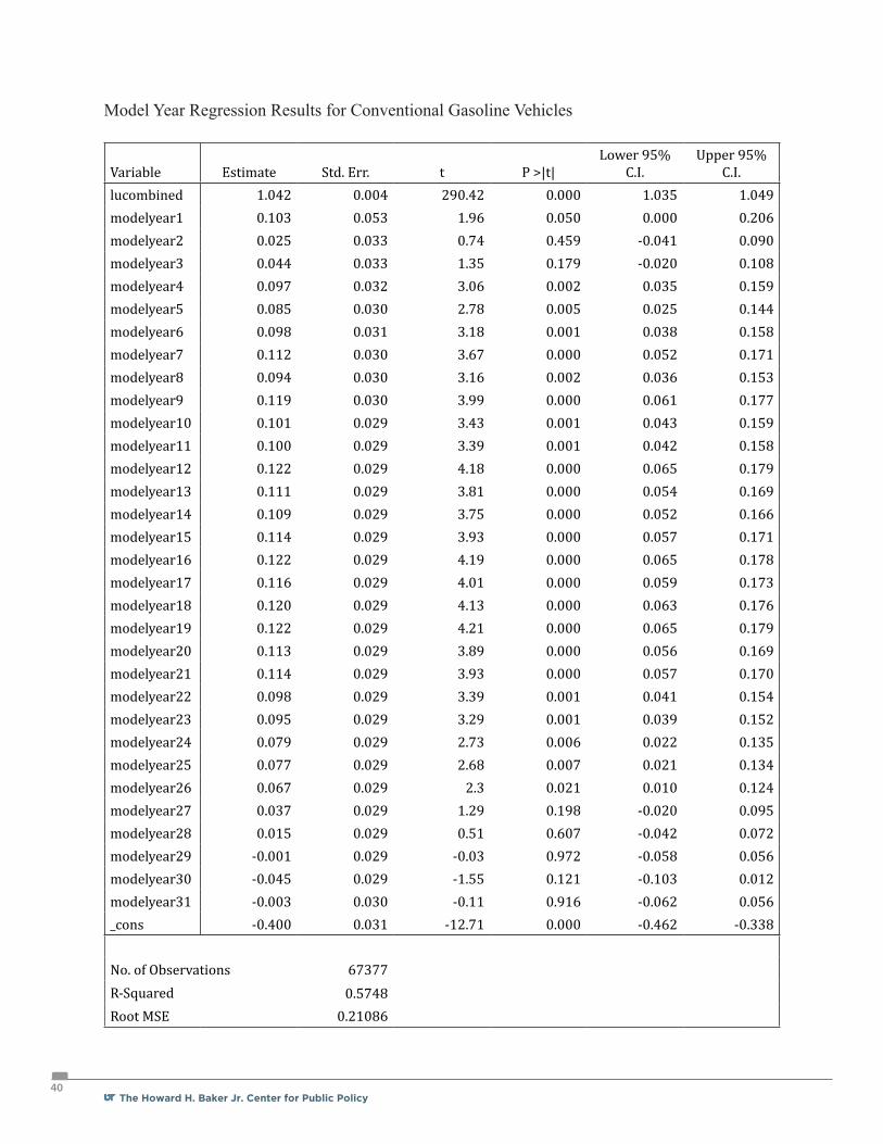
The Howard H. Baker Jr. Center for Public Policy40
Model Year Regression Results for Conventional Gasoline Vehicles
Variable Estimate Std. Err. t P >|t|Lower 95%
C.I.Upper 95%
C.I.lucombined 1.042 0.004 290.42 0.000 1.035 1.049modelyear1 0.103 0.053 1.96 0.050 0.000 0.206modelyear2 0.025 0.033 0.74 0.459 -0.041 0.090modelyear3 0.044 0.033 1.35 0.179 -0.020 0.108modelyear4 0.097 0.032 3.06 0.002 0.035 0.159modelyear5 0.085 0.030 2.78 0.005 0.025 0.144modelyear6 0.098 0.031 3.18 0.001 0.038 0.158modelyear7 0.112 0.030 3.67 0.000 0.052 0.171modelyear8 0.094 0.030 3.16 0.002 0.036 0.153modelyear9 0.119 0.030 3.99 0.000 0.061 0.177modelyear10 0.101 0.029 3.43 0.001 0.043 0.159modelyear11 0.100 0.029 3.39 0.001 0.042 0.158modelyear12 0.122 0.029 4.18 0.000 0.065 0.179modelyear13 0.111 0.029 3.81 0.000 0.054 0.169modelyear14 0.109 0.029 3.75 0.000 0.052 0.166modelyear15 0.114 0.029 3.93 0.000 0.057 0.171modelyear16 0.122 0.029 4.19 0.000 0.065 0.178modelyear17 0.116 0.029 4.01 0.000 0.059 0.173modelyear18 0.120 0.029 4.13 0.000 0.063 0.176modelyear19 0.122 0.029 4.21 0.000 0.065 0.179modelyear20 0.113 0.029 3.89 0.000 0.056 0.169modelyear21 0.114 0.029 3.93 0.000 0.057 0.170modelyear22 0.098 0.029 3.39 0.001 0.041 0.154modelyear23 0.095 0.029 3.29 0.001 0.039 0.152modelyear24 0.079 0.029 2.73 0.006 0.022 0.135modelyear25 0.077 0.029 2.68 0.007 0.021 0.134modelyear26 0.067 0.029 2.3 0.021 0.010 0.124modelyear27 0.037 0.029 1.29 0.198 -0.020 0.095modelyear28 0.015 0.029 0.51 0.607 -0.042 0.072modelyear29 -0.001 0.029 -0.03 0.972 -0.058 0.056modelyear30 -0.045 0.029 -1.55 0.121 -0.103 0.012modelyear31 -0.003 0.030 -0.11 0.916 -0.062 0.056_cons -0.400 0.031 -12.71 0.000 -0.462 -0.338 No. of Observations 67377 R-Squared 0.5748 Root MSE 0.21086