1

Project Number: MA-WJM-9800

Semidefinite Programming and its Application to the Sensor Network Localization Problem

A Major Qualifying Project Report

submitted to the Faculty

of the

WORCESTER POLYTECHNIC INSTITUTE

in partial fulfillment of the requirements for the

Degree of Bachelor of Science

by

_______________________________

Elizabeth A. Hegarty

Date: April 29, 2010

Approved:

______________________________________

Professor William J. Martin, Major Advisor

2

Abstract

Semidefinite programming is a recently developed branch of convex optimization. It is an exciting, new topic in mathematics, as well as other areas, because of its algorithmic efficiency and broad applicability. In linear programming, we optimize a linear function subject to linear constraints. Semidefinite programming, however, addresses the optimization of a linear function subject to nonlinear constraints. The most important of these constraints requires that a combination of symmetric matrices be positive semidefinite. In spite of the presence of nonlinear constraints, several efficient methods for the numerical solution of semidefinite programming problems (SDPs) have emerged in recent years, the most common of which are interior point methods. With these methods, not only can SDPs be solved in polynomial time in theory, but the existing software works very well in practice.

About the same time these efficient algorithms were being developed, very exciting applications of semidefinite programming were discovered. With its use, experts were able to find approximations to NP-Complete problems that were .878 of the actual solution. This is amazing considering for some NP-Complete problems we cannot even find approximations that are 1% of the actual solution. Another amazing result was in coding theory. By applying semidefinite programming, the first advancement in 30 years was made on the upper bound of the maximum number of code words needed. Other great outcomes have arisen in areas such as eigenvalue optimization, civil engineering, sensor networks, and the financial sector, proving semidefinite programming to be a marvelous tool for all areas of study.

This project focuses on the understanding of semidefinite programming and its application to sensor networks. I began first by learning the theory of semidefinite programming and of the interior point methods which solve SDPs. Next, I surveyed many recent applications of semidefinite programming and chose the sensor network localization problem (SNLP) as a case study. I then implemented the use of an online tool -- the algorithm csdp, from the NEOS Solvers website -- to solve given SNLPs. I also developed MAPLE code to aid in the process of transforming a naturally stated problem into one suitable for NEOS input and for interpreting the csdp solution in a way understandable to a user unfamiliar with advanced mathematics.

3

Contents 1 Introduction .......................................................................................................................................... 4

1.1 Notation ........................................................................................................................................ 5

2 Semidefinite Programming ................................................................................................................... 7

2.1 Background Theory ....................................................................................................................... 8

2.2 Semidefinite Programming Theory ............................................................................................. 12

2.3 The Interior Point Method .......................................................................................................... 15

2.3.1 The Central Path .................................................................................................................. 15

2.3.2 Interior Point Method for Semidefinite Programming ....................................................... 25

2.3.3 Descent Direction ................................................................................................................ 35

3 Survey of Applications......................................................................................................................... 37

3.1 Famous Applications ...................................................................... Error! Bookmark not defined.

3.1.1 Max-Cut ............................................................................................................................... 37

3.1.2 Max-2-SAT ........................................................................................................................... 41

3.1.3 Schrijver Coding Theory ...................................................................................................... 41

3.1.4 Lewis’ Eigenvalue Optimization ............................................. Error! Bookmark not defined.

3.1.5 Financial Application .............................................................. Error! Bookmark not defined.

3.2 The Sensor Network Localization Problem ................................................................................. 43

3.2.1 Constructing the Problem ................................................................................................... 44

3.2.2 Methods for Solving ............................................................................................................ 44

4 NEOS Guide ......................................................................................................................................... 49

4.1 NEOS Input and Output .............................................................................................................. 49

4.1.1 Input .................................................................................................................................... 49

4.1.2 Output ................................................................................................................................. 52

4.2 MAPLE CODES ............................................................................................................................. 52

4.2.1 Data File .............................................................................................................................. 53

4.2.2 MAPLE Code 1: Data to NEOS Input .................................................................................... 54

4.2.3 MAPLE Code 2: NEOS Output to Matrix and Graph ............................................................ 59

5 Conclusion and Further Work ............................................................................................................. 66

6 References .......................................................................................................................................... 67

4

1 Introduction

In the 1990s, a new development in mathematical sciences was made which allowed for broad

applicability and great advances in many areas of study. This development was of semidefinite

programming, a branch of convex optimization which can optimize linear functions given constraints

that are nonlinear and involving positive semidefinite matrices. The results of this development were

greater than could be imagined, with more exciting advancements continuing to be made today. Experts

were able to find approximations to NP-Complete problems that were . 878 of the actual solution. This

is amazing considering for some NP-Complete problems we cannot even find approximations that are

1% of the actual solution. Another amazing result made possible by semidefinite programming was in

the field of coding theory. With semidefinite programming, the first advancement in 30 years on the

upper bound of the maximum number of code words needed was made possible. Other great outcomes

have stemmed from semidefinite programming, such as its use in civil engineering and the financial

sector, proving it to be a marvelous tool for all areas of study.

The general semidefinite programming problem (SDP) optimizes the trace of the product of two

matrices, one being the variable matrix, 𝑋. One set of constraints require that the difference between a

vector and a linear operator be zero, while the other set requires this difference to be nonnegative. The

last constraint is that the variable matrix, 𝑋, be positive semidefinite. This is where we lose the linearity

of our system. However, these constraints are still convex, allowing semidefinite programming to fall

under convex optimization. Also, while SDPs are not linear programming problems (LPs), every LP can be

relaxed into a SDP.

For every SDP, one can obtain the dual with the use of Lagrange multipliers. This ability led to

adaptations of the Weak Duality Theorem and the Complementary Slackness Theorem to semidefinite

programming. In the cases where we have strictly feasible interior points for the primal and dual

problems, the Strong Duality Theorem can also be applied. These theorems aid in guaranteeing the

solution obtained is the optimal solution. However, since semidefinite programming contains nonlinear

constraints, one cannot use linear programming techniques to obtain this optimal solution. For this

reason, methods for solution have been researched with many techniques being successful. In 1996,

Christoph Helmberg, Franz Rendl, Robert Vanderbei and Henry Wolkowicz introduced an interior point

method for SDPs, utilizing ideas of advanced linear programming. These ideas were of the central path

and the path following method, which involve the use of barrier functions, Lagrangians, first- order

optimality conditions, and Newton’s method. Helmberg et al. were able to adapt all of these ideas to

semidefinite programming, obtaining a very efficient algorithm for numerical solution. Many computer

programs have been written for this algorithm and work very well in practice.

As noted previously, semidefinite programming’s great appeal comes from its broad applicability. One

very prominent application, which is worth elaborating on, is its use in sensor networks. Sensor

networks are used to collect information on the environment they are placed in, however this

information is only relevant if the positions of all the sensors are known. The problem of locating all of

the sensors is identified as the Sensor Network Localization Problem (SNLP). Through the use of distance

measurements and some known sensor positions, semidefinite programming can locate all the positions

5

of the sensors in the system. Through use of computer programs, SNLPs can be solved quickly and

efficiently.

This application, along with many others, can allow for semidefinite programming to become significant

even to those not involved in advanced areas of study. While semidefinite programming seems like just

another topic in mathematics whose purpose in everyday life and that of the common person seems

meager, many of these applications can impact our lives. Its application in coding theory could lead to

the shortening of codes which are used in almost everything from CDs to cell phones to the internet.

The shortened code length would result in our whole world working much faster. Semidefinite

programming and the SNLP can be utilized for military purposes, allowing for aerial deployment and the

collection of information, such as air content and positioning of enemy lines, during ground warfare. The

ability to solve the SNLP with semidefinite programming also intrigues many people for its use with

firefighters. Being able to know the positions of firefighters inside a burning building and the

environmental conditions they are in could lead to much greater safety for all involved because more

informed decisions could be made. This application has become a very prevalent research topic at

Worcester Polytechnic Institute, hoping to develop easy to use techniques to prevent firefighter injuries

and casualties.

This report focuses on the understanding of semidefinite programming and its use in the field of sensor

networks. I finish this section by introducing some notation. In the second chapter, I discuss the ideas of

semidefinite programming. I begin by presenting the theory behind SDPs and then explain the interior

point method developed by Helmberg et al. for numerical solution. In the third chapter, I discuss the

uses of SDPs by first presenting a survey of famous applications. I then explore semidefinite

programming’s use in the SNLP. Finally, in the last chapter, I present a guide for utilizing the NEOS

Solvers (an online tool for optimization problems) for solving SNLPs and MAPLE codes to aid in the

process.

1.1 Notation

The main point of this section is to introduce some notation and define some of the major terms this

paper is going to use. Those presented here will be the most common, and while some may be a review,

a good understanding of the ideas is needed in order to continue. Note that if an idea is not discussed

here and is used later on, it will be defined at the time of its use.

To begin I will introduce the notation for the inner product. This is 𝑥, 𝑦 and, as part of its definition,

𝑥, 𝑦 = 𝑥𝑇𝑦. From here, I will define the trace of a matrix. This is the addition of the diagonal entries of

a square matrix. In this paper, we will often want to obtain the trace of the product of two matrices,

one being the transpose of a matrix. Since, in semidefinite programming this trace will be the inner

product we use, we will denote it as: 𝑡𝑟(𝐹𝑇𝐺) = 𝐹, 𝐺 .

Next, while positive semidefinite matrices will be defined later, this paper will denote them using this

symbol: ≽. For example, if a matrix 𝐴 is positive semidefinite we will say that 𝐴 ≽ 0. We will do similarly

for a positive definite matrix but instead use this symbol: ≻.

6

In the general SDP system, we utilize the terms 𝐴(𝑋) and 𝐵(𝑋). These will be linear operators which

take our variable matrix 𝑋 and a set of 𝑘 matrices 𝐴𝑖 (a set of 𝑚 matrices 𝐵𝑖 for the linear operator

𝐵(𝑋)) and lists the traces of 𝑋 with each matrix 𝐴𝑖 in a vector. For each of these linear operators, there

is an adjoint linear operator which takes the list and maps it back on to the matrices. We will denote

these as 𝐴𝑇(𝑋) and 𝐵𝑇(𝑋). These adjoints are defined by this relation: 𝐴 𝑋 , 𝑦 = 𝑋, 𝐴𝑇(𝑦) .

We will begin our discussion with the basic theory. We will denote a vector by placing an arrow above it.

For example, 𝑢 . However, once we get into defining the system, we can drop this notation because we

do not run into situations in which this could get confusing. We will be using the terms 𝑎, 𝑏, 𝑦, and 𝑡 in

our systems which will all be vectors. The vectors 𝑎 and 𝑦 will be of length 𝑘 and the vectors 𝑏 and 𝑡 will

be of length 𝑚.

Lastly, we will quickly note a few things. We will use 𝒞 to denote a cone, 𝑒 will be the all ones vector,

and 𝐴 ∘ 𝐵 will be the entrywise product of 𝐴 and 𝐵.

7

2 Semidefinite Programming

Semidefinite programming is a newly developed branch of conic programming. To begin, we will discuss

this over arching subject. Conic programming works in a Euclidean space. By a Euclidean space, we mean

a vector space, 𝐸, over ℝ with positive definite inner product. A positive definite inner product refers to

the case where, for 𝑥 ∈ 𝐸, 𝑥, 𝑥 ≥ 0 and only equals zero if 𝑥 is the zero vector. A cone in 𝐸 is any

subset closed under addition and multiplication by non-negative scalars. That is 𝒞 ⊆ 𝐸 is a cone if the

following hold:

∀ 𝑥, 𝑦 ∈ 𝒞, 𝑥 + 𝑦 ∈ 𝒞

∀ 𝑥 ∈ 𝒞 𝑎𝑛𝑑 ∀ 𝛽 ≥ 0, 𝛽𝑥 ∈ 𝒞

A conic programming problem optimizes a linear function over a linear section of some cone. A general

conic programming problem takes the following form:

max 𝐶, 𝑋

𝑠𝑡 𝐴𝑖 , 𝑋 = 𝑏𝑖 , 1 ≤ 𝑖 ≤ 𝑚

𝑥 ∈ 𝒞

Let us consider two special cases of conic programming. One is linear programming in which the vector

space 𝐸 is equal to ℝ𝑛 . A general linear programming problem (LP) is:

max 𝑐𝑇𝑥

𝑠𝑡 𝑎𝑖𝑇𝑥 = 𝑏𝑖

𝑥 ≥ 0

One can see that the objective function is equivalent to the conic programming problem above, noting

the definition of an inner product, 𝑥, 𝑦 = 𝑥𝑇𝑦. The cone in which we are optimizing over requires all

the entries of 𝑥 are nonnegative.

Another special case is semidefinite programming, our main topic for discussion. In this case, the vector

space is of 𝑛 𝑥 𝑛 symmetric matrices. The general semidefinite programming problem (SDP) is as

follows:

max 𝐶, 𝑋

𝑠𝑡 𝐴𝑖 , 𝑋 = 𝑏𝑖

𝑋 ≽ 0

Here we take the inner product to be the trace of the product of two matrices, one being a transpose.

For example, 𝐶, 𝑋 = 𝑡𝑟(𝐶𝑇𝑋). The cone we are use in the SDP is one which requires matrices to be

positive semidefinite.

8

It can be shown that all LPs can be relaxed into SDPs. The idea is simple in that we think of the vectors

used in LPs as just 1 𝑥 𝑛 matrices, allowing us to refer to 𝑐 as𝐶, 𝑥 as𝑋, and 𝑎𝑖 as 𝐴𝑖 . With this idea we

can see that 𝐶, 𝑋 = 𝑡𝑟(𝐶𝑇𝑋) will just become the trace of a 1 𝑥 1 matrix, or just a single value, and

this value will be the inner product of the vectors 𝑐 and 𝑥. We can also see that the vector 𝑥, or the

1 𝑥 𝑛 matrix 𝑋, will be positive semidefinite because we all the entries of 𝑥 need to be nonnegative.

2.1 Background Theory

To discuss semidefinite programming further we need to introduce some background theory that will

lead us to defining semidefinite matrices and understanding their properties.

Let 𝐴 be a real symmetric 𝑛 𝑥 𝑛 matrix. We know that 𝜆 ∈ ℂ (where ℂ is the set of complex numbers) is

an eigenvalue of 𝐴 if there is a nonzero 𝑣 ∈ ℂ𝑛 𝑠. 𝑡. 𝐴𝑣 = 𝜆𝑣 . If this holds then not only is 𝜆 an

eigenvalue but 𝑣 is an eigenvector.

If 𝑀 is a 𝑛 𝑥 𝑛 matrix over the complex numbers, then 𝑀† is the conjugate transpose of 𝑀. For example:

𝐿𝑒𝑡 𝑀 = 1 − 𝑖 𝑖

2 3 𝑡𝑕𝑒𝑛 𝑀† =

1 + 𝑖 2−𝑖 3

M is called Hermitean if and only if 𝑀† = 𝑀. In the case that 𝑀 is a matrix over the Reals then it is

Hermitean if and only if 𝑀 is symmetric.

These two ideas are utilized in our first lemma:

Lemma 1: Every eigenvalue of any Hermitean matrix is real.

Let us prove this:

First we recall the definition of the inner product, ∙,∙ on ℂ as 𝑢 , 𝑣 = 𝑢 𝑇𝑣 = 𝑢 𝑖𝑣𝑖𝑛𝑖=1

(where 𝑢 is the complex conjugate)

We know that 𝑀 is Hermitean and suppose 𝜆 is an eigenvalue for some nonzero vector 𝑢 , then

𝑀𝑢 = 𝜆𝑢 .

Also, from the above definition, we can say:

𝜆 𝑢 , 𝑢 = 𝜆 𝑢 𝑇𝑢 = 𝑢 𝑇 𝜆𝑢 = 𝑢 𝑇 𝑀𝑢 = (𝑢 𝑇𝑀†)𝑢

= (𝑀𝑢 )𝑇𝑢 = 𝑀𝑢 , 𝑢 = 𝜆𝑢 , 𝑢 = 𝜆 𝑢 , 𝑢

So we have that 𝜆 𝑢 , 𝑢 = 𝜆 𝑢 , 𝑢 which means that 𝜆 = 𝜆 since 𝑢 , 𝑢 ≠ 0. This means that 𝜆 is

real.

𝑁𝑜𝑡𝑒: 𝑎 + 𝑏𝑖 = 𝑎 − 𝑏𝑖 𝑖𝑓 𝑎𝑛𝑑 𝑜𝑛𝑙𝑦 𝑖𝑓 𝑏𝑖 = 0

9

This means that every eigenvalue of a Hermitean matrix is real.∎

Our second lemma discusses more properties using eigenvalues.

Lemma 2: If 𝐴 is a real symmetric matrix, then eigenvectors belonging to distinct eigenvalues are

orthogonal.

The proof is as follows:

Let 𝐴𝑢 = 𝜆𝑢 𝑎𝑛𝑑 𝐴𝑣 = 𝜇𝑣 𝑤𝑕𝑒𝑟𝑒 𝜆 ≠ 𝜇

Consider 𝜆 𝑢 , 𝑣 = (𝜆𝑢 )𝑇𝑣 :

𝜆 𝑢 , 𝑣 = (𝜆𝑢 )𝑇𝑣 = (𝐴𝑢 )𝑇𝑢 = 𝑢 𝑇𝐴𝑇𝑣 = 𝑢 𝑇𝐴𝑣 = 𝑢 𝑇 𝜇𝑣 = 𝜇 𝑢 , 𝑣

So we have that 𝜆 𝑢 , 𝑣 = 𝜇 𝑢 , 𝑣 and since we know that 𝜆 ≠ 𝜇 because they are distinct

eigenvalues, then that means 𝑢 , 𝑣 = 0. This only occurs if 𝑢 is orthogonal to 𝑣 . ∎

This third lemma discusses linear transformations.

Lemma 3: Every linear transformation 𝑇: 𝑉 → 𝑉 has a real eigenvalue, where 𝑇 is a finite-

dimensional, real vector space.

Proof:

Coordinize 𝑉 so that 𝑇 𝑥 = 𝐴𝑥 for some 𝑛 𝑥 𝑛 matrix 𝐴 where 𝑛 is also the dimension of 𝑉.

The characteristic polynomial for 𝑇 𝑥 is 𝒳𝑇 𝜆 = 𝑑𝑒𝑡(𝜆𝐼 − 𝐴) which is a polynomial of degree

𝑛 in λ with real coefficients.

From the Fundamental Theorem of Algebra, we know that every non-constant polynomial has a

root. This is true for complex numbers with polynomial of positive degree.

So for some 𝜃 ∈ ℂ, 𝒳𝑇 𝜃 = 0. This means that 𝑑𝑒𝑡 𝜃𝐼 − 𝐴 = 0.

So ∃𝑣 ≠ 0 𝑠. 𝑡. 𝜃𝐼 − 𝐴 𝑣 = 0 ⟹ 𝐴𝑣 = 𝜃𝑣

This means that 𝑣 is an eigenvector for 𝐴, hence for𝑇, and 𝜃 is an eigenvalue for 𝐴 and 𝑇.

By Lemma 1, this means that 𝜃 is real. ∎

These three lemmas lead us to our first main theorem.

Theorem 1: If 𝐴 is a real symmetric 𝑛 𝑥 𝑛 matrix then 𝐴 is orthogonally diagonalizable, i.e.

there exists orthogonal 𝑃 and diagonal 𝐷 s.t. 𝐴 = 𝑃𝐷𝑃𝑇 , 𝑖. 𝑒. 𝐴𝑃 = 𝑃𝐷.

10

The proof is done by induction:

Let 𝑇: ℝ𝑛 → ℝ𝑛 by 𝑇 𝑥 = 𝐴𝑥

Then 𝑇 has an eigenvector 𝑣 1 ∈ ℝ𝑛 so 𝐴𝑣 1 = 𝜃𝑣 1 for some 𝜃 ∈ ℝ

Consider 𝑊 = 𝑣 1⊥ = 𝑤 ∈ 𝑉: 𝑤 , 𝑣 1 = 0

We claim: 𝑤 → 𝐴𝑤 is a linear transformation 𝑇 ′ = 𝑊 → 𝑊

Proof: If 𝑤 ⊥ 𝑣 1 ⟹ 𝐴𝑤 ⊥ 𝑣 1

𝐴𝑤 , 𝑣 1 = 𝑤 , 𝐴𝑣 1 = 𝜃 𝑤 , 𝑣 1 = 0

⟹ 𝐴𝑤 ⊥ 𝑣 1

By induction, 𝑊 has an orthogonal basis of eigenvectors for 𝑇 ′ . ∎

The next two theorems will be quickly noted allowing us to finally arrive at our definitions for positive

semidefinite and positive definite matrices. The first theorem builds on Theorem 1 to further describe

properties of symmetric 𝑛 𝑥 𝑛 matrices.

Theorem 2: Every symmetric 𝑛 𝑥 𝑛 matrix 𝐴 is orthogonally similar to a diagonal matrix.

The second is the Spectral Decomposition Theorem.

Theorem 3: For any real symmetric 𝑛 𝑥 𝑛 matrix, there exists real numbers 𝜃1, 𝜃2 , ……𝜃𝑛 and

orthonormal basis 𝑣1 , 𝑣2 , ……𝑣𝑛 such that

𝐴 = 𝜃1𝑣1𝑣1𝑇 + 𝜃2𝑣2𝑣2

𝑇 + ⋯ + 𝜃𝑛𝑣𝑛𝑣𝑛𝑇 = 𝜃𝑗𝑣𝑗𝑣𝑗

𝑇

𝑛

𝑗 =1

We now have the background to introduce positive semidefinite matrices and discuss some of their

properties.

Positive semidefinite (PSD): A real symmetric matrix 𝐴 is positive semidefinite if ∀𝑣 ∈ ℝ𝑛 , 𝑣 𝑇𝐴𝑣 ≥ 0.

Positive definite (PD): A real symmetric matrix 𝐵 is positive definite (PD) if ∀𝑣 ∈ ℝ𝑛 , 𝑣 ≠ 0, 𝑣 𝑇𝐵𝑣 > 0.

Here are some examples:

𝑃𝐷 𝐴1 = 1 0 000

2 00 3

, 𝑃𝑆𝐷 𝐴2 = 1 0 000

2 00 0

, 𝑛𝑜𝑡 𝑃𝑆𝐷 𝐴3 = 1 0 000

2 00 −3

We can prove these are true with the defining equations. We will show this for the first matrix:

11

First we can see that 𝐴1 is a real symmetric matrix.

Second, we need ∀𝑣 ∈ ℝ𝑛 , 𝑣 ≠ 0, 𝑣 𝑇𝐴𝑣 > 0.

We define 𝑣 =

𝑣1

𝑣2

𝑣3

and we have 𝐴1 = 1 0 000

2 00 3

.

So 𝑣 𝑇𝐴1𝑣 = 𝑣12 + 2𝑣2

2 + 3𝑣32 which is > 0 unless 𝑣1 , 𝑣2 , 𝑣3 = 0. So 𝐴1 is PD.

This brings us to our fourth theorem.

Theorem 4: Let 𝐴 be a symmetric 𝑛 𝑥 𝑛 real matrix then

1. 𝐴 is PSD if and only if all eigenvalues of 𝐴 are non-negative

2. 𝐴 is PD if and only if all eigenvalues of 𝐴 are positive

We will do the proof of the first part of the theorem (the second part is very similar)

(⟹) Assume that 𝐴 is PSD and 𝐴𝑢 = 𝜆𝑢 , 𝑢 ≠ 0 . Then have 𝑢 𝑇𝐴𝑢 = 𝜆𝑢 𝑇𝑢 by multiplying both

sides by 𝑢 𝑇 . But 𝑢 𝑇𝐴𝑢 ≥ 0 because 𝐴 is PSD and 𝑢 𝑇𝑢 > 0 so this means that 𝜆 ≥ 0.

(⟸) Assume all eigenvalues are non-negative. We can write 𝐴 as 𝐴 = 𝑃𝐷𝑃𝑇 from our first

theorem. So 𝐷 is diagonal with all entries non-negative. Also note, for any vector 𝑢 ,

𝑢 𝑇𝐷𝑢 = 𝐷𝑖𝑖𝑢𝑖2 which will always be positive.

We can now write 𝑣 𝑇𝐴𝑣 as 𝑣 𝑇𝑃𝐷𝑃𝑇𝑣 and see that

𝑣 𝑇𝐴𝑣 = 𝑣 𝑇𝑃𝐷𝑃𝑇𝑣 = 𝑃𝑇𝑣 𝑇𝐷(𝑃𝑇𝑣 ) ≥ 0

which means that 𝐴 is PSD. ∎

At this point, we will introduce the idea of a principal submatrix which is composed from a larger, square

matrix. A principal submatrix of a 𝑛 𝑥 𝑛 matrix 𝐴 is any 𝑚 𝑥 𝑚 submatrix obtained from 𝐴 by deleting

𝑛 − 𝑚 rows and the corresponding columns. Our last theorem shows the relationship between these

principal submatrices and PSD matrices.

Theorem 5: Everyone principal submatrix of a positive semidefinite matrix A is also positive

semidefinite.

These theorems and lemmas provide the background for semidefinite programming. With their

understanding, we will be able to further understand the ideas presented next.

12

2.2 Semidefinite Programming Theory

With all of the background introduced, we can continue our discussion of semidefinite programming.

The general system is as follows:

SDP

𝑀𝑎𝑥 𝐶, 𝑋

𝑠. 𝑡. 𝐴 𝑋 = 𝑎

𝐵 𝑋 ≤ 𝑏

𝑋 ≽ 0

𝑊𝑕𝑒𝑟𝑒 𝐴 𝑋 =

𝑡𝑟(𝐴1𝑋)𝑡𝑟(𝐴2𝑋)

⋮𝑡𝑟(𝐴𝑘𝑋)

𝑎𝑛𝑑 𝐵 𝑋 =

𝑡𝑟(𝐵1𝑋)𝑡𝑟(𝐵2𝑋)

⋮𝑡𝑟(𝐵𝑘𝑋)

We can obtain the dual of this system fairly easily. The process is explained [1].

We start by letting 𝑣∗ equal the optimal value for the SDP and introducing Lagrange multipliers 𝑦 ∈ ℝ𝑘

for the equality constraint and 𝑡 ∈ ℝ𝑚 for the inequality constraint.

We can then say that

𝑣∗ = 𝑚𝑎𝑥𝑋≽0𝑚𝑖𝑛𝑡≥0,𝑦 𝑡𝑟𝐶𝑋 + 𝑦𝑇 𝑎 − 𝐴 𝑋 + 𝑡𝑇(𝑏 − 𝐵 𝑋 ).

This will be less than the optimal solution for the dual which is equal to

𝑚𝑖𝑛𝑡≥0,𝑦𝑚𝑎𝑥𝑋≽0 𝑡𝑟 𝐶 − 𝐴𝑇 𝑦 − 𝐵𝑇 𝑡 𝑋 + 𝑎𝑇𝑦 + 𝑏𝑇𝑡.

Note that the inner max over 𝑋 is bounded from above only if 𝐴𝑇 𝑦 + 𝐵𝑇 𝑡 − 𝐶 ≥ 0 and the

maximum happens when 𝑡𝑟 𝐶 − 𝐴𝑇 𝑦 − 𝐵𝑇 𝑡 𝑋 = 0. So we can just say that we need to min over

the rest of the function when this term is zero. This presents us with our D-SDP shown below.

D-SDP

𝑀𝑖𝑛 𝑎𝑇𝑦 + 𝑏𝑇𝑡

𝑠. 𝑡. 𝐴𝑇 𝑦 + 𝐵𝑇 𝑡 − 𝐶 ≽ 0

𝑡 ≥ 0

𝑊𝑕𝑒𝑟𝑒 𝐴𝑇 𝑦 = 𝑦𝑖𝐴𝑖

𝑘

𝑖=1

𝑎𝑛𝑑 𝐵𝑇 𝑡 = 𝑡𝑖𝐵𝑖

𝑙

𝑖=1

13

Recall that in linear programming, we have a Weak Duality Theorem. This theorem can be adapted to

semidefinite programming. The Weak Duality Theorem for SDP is stated below.

Weak Duality Theorem: If 𝑋 is feasible for the SDP and (𝑦, 𝑡, 𝑍) is feasible for the D-SDP,

then 𝐶, 𝑋 ≤ 𝑦𝑇𝑎 + 𝑡𝑇𝑏.

The proof of this is as follows:

First we need to note that for 𝑋 and 𝑦, 𝑡, 𝑍 to be feasible, then 𝑋 ≽ 0, 𝑍 ≽ 0 meaning that

𝑍, 𝑋 ≥ 0.

We can obtain 𝐶 from the first constraint in the dual SDP and plug that into 𝐶, 𝑋 :

𝐶, 𝑋 = 𝑦𝑖𝐴𝑖 𝑘𝑖=1 + 𝑡𝑖𝐵𝑖

𝑙𝑖=1 − 𝑍 , 𝑋 = 𝑦𝑖 𝐴𝑖 , 𝑋 𝑘

𝑖=1 + 𝑡𝑖 𝐵𝑖 , 𝑋 𝑙𝑖=1 − 𝑍, 𝑋

But we know, since 𝑋 and (𝑦, 𝑡, 𝑍)are both feasible, then the constraints hold. That means that:

𝐴𝑖 , 𝑋 = 𝑎 𝑎𝑛𝑑 𝐵𝑖 , 𝑋 ≤ 𝑏

So we can write:

𝐶, 𝑋 = 𝑦𝑖 𝐴𝑖 , 𝑋

𝑘

𝑖=1

+ 𝑡𝑖 𝐵𝑖 , 𝑋

𝑙

𝑖=1

− 𝑍, 𝑋 ≤ 𝑦𝑖𝑎𝑖

𝑘

𝑖=1

+ 𝑡𝑖𝑏𝑖

𝑙

𝑖=1

− 𝑍, 𝑋

Since we have that 𝑍, 𝑋 ≥ 0, then we can conclude that:

𝑦𝑖𝑎𝑖

𝑘

𝑖=1

+ 𝑡𝑖𝑏𝑖

𝑙

𝑖=1

− 𝑍, 𝑋 ≤ 𝑦𝑖𝑎𝑖

𝑘

𝑖=1

+ 𝑡𝑖𝑏𝑖

𝑙

𝑖=1

= 𝑦𝑇𝑎 + 𝑡𝑇𝑏

So we have that 𝐶, 𝑋 ≤ 𝑦𝑇𝑎 + 𝑡𝑇𝑏. ∎

Similarly, we have a form of the Complementary Slackness Theorem for semidefinite programming. It is

as follows:

Complementary Slackness Theorem: If 𝑋 is optimal for SDP, (𝑦, 𝑡, 𝑍) is optimal for D-SDP and

𝐶, 𝑋 = 𝑦𝑇𝑎 + 𝑡𝑇𝑏 then

1. 𝑇𝑟 𝑍𝑋 = 0

2. For every 𝑖, 1 ≤ 𝑖 ≤ 𝑙, 𝑡𝑖 = 0 or 𝐵𝑖 , 𝑋 = 𝑏𝑖

Here is the proof:

1. 𝐶, 𝑋 = 𝑦𝑖𝐴𝑖 𝑘𝑖=1 + 𝑡𝑖𝐵𝑖

𝑙𝑖=1 − 𝑍 , 𝑋 = 𝑦𝑖 𝐴𝑖 , 𝑋 𝑘

𝑖=1 + 𝑡𝑖 𝐵𝑖 , 𝑋 𝑙𝑖=1 − 𝑍, 𝑋

We can move things around to arrive at:

14

𝑍, 𝑋 = 𝑦𝑖 𝐴𝑖 , 𝑋

𝑘

𝑖=1

+ 𝑡𝑖 𝐵𝑖 , 𝑋

𝑙

𝑖=1

− 𝐶, 𝑋

We have that 𝐴𝑖 , 𝑋 = 𝑎𝑖 𝑎𝑛𝑑 𝐵𝑖 , 𝑋 ≤ 𝑏𝑖 so

𝑍, 𝑋 ≤ 𝑦𝑖𝑎𝑖

𝑘

𝑖=1

+ 𝑡𝑖𝑏𝑖

𝑙

𝑖=1

− 𝐶, 𝑋 = 𝑦𝑇𝑎 + 𝑡𝑇𝑏 − 𝐶, 𝑋

But 𝐶, 𝑋 = 𝑦𝑇𝑎 + 𝑡𝑇𝑏 from assumption that 𝑋 and (𝑦, 𝑡, 𝑍) are optimal.

So 𝑍, 𝑋 ≤ 𝑦𝑇𝑎 + 𝑡𝑇𝑏 − 𝐶, 𝑋 = 0 which means that 𝑍, 𝑋 ≤ 0.

But since 𝑍 ≽ 0 and 𝑋 ≽ 0 then 𝑍, 𝑋 ≥ 0

So 𝑍, 𝑋 = 𝑇𝑟 𝑍𝑋 = 0

2. We know that 𝐶, 𝑋 = 𝑦𝑖 𝐴𝑖 , 𝑋 𝑘𝑖=1 + 𝑡𝑖 𝐵𝑖 , 𝑋 𝑙

𝑖=1 − 𝑍, 𝑋 but from above, we have

that 𝑍, 𝑋 = 0 so we can drop this term.

This leaves us with 𝐶, 𝑋 = 𝑦𝑖 𝐴𝑖 , 𝑋 𝑘𝑖=1 + 𝑡𝑖 𝐵𝑖 , 𝑋 𝑙

𝑖=1

But since 𝐵 𝑋 ≤ 𝑏, then

𝐶, 𝑋 = 𝑦𝑖 𝐴𝑖 , 𝑋

𝑘

𝑖=1

+ 𝑡𝑖 𝐵𝑖 , 𝑋

𝑙

𝑖=1

≤ 𝑦𝑖𝑎𝑖

𝑘

𝑖=1

+ 𝑡𝑖𝑏𝑖

𝑙

𝑖=1

= 𝑦𝑇𝑎 + 𝑡𝑇𝑏

But by assumption that 𝑋 and (𝑦, 𝑡, 𝑍) are optimal, then 𝐶, 𝑋 = 𝑦𝑇𝑎 + 𝑡𝑇𝑏.

This means that this must hold:

𝑦𝑖 𝐴𝑖 , 𝑋

𝑘

𝑖=1

+ 𝑡𝑖 𝐵𝑖 , 𝑋

𝑙

𝑖=1

= 𝑦𝑖𝑎𝑖

𝑘

𝑖=1

+ 𝑡𝑖𝑏𝑖

𝑙

𝑖=1

Since we know by the constraints that 𝐴𝑖 , 𝑋 = 𝑎𝑖 , it obviously follows that

𝑦𝑖 𝐴𝑖 , 𝑋

𝑘

𝑖=1

= 𝑦𝑖𝑎𝑖

𝑘

𝑖=1

What we really need is that

𝑡𝑖 𝐵𝑖 , 𝑋

𝑙

𝑖=1

= 𝑡𝑖𝑏𝑖

𝑙

𝑖=1

By the constraints, we have 𝐵𝑖 , 𝑋 ≤ 𝑏𝑖 . This gives us two cases:

1. If 𝐵𝑖 , 𝑋 < 𝑏𝑖 , then we must have that 𝑡𝑖 = 0, ∀𝑖 in order for the equality to hold

2. If 𝐵𝑖 , 𝑋 = 𝑏𝑖 , then the equality obviously holds

So for 𝐶, 𝑋 = 𝑦𝑇𝑎 + 𝑡𝑇𝑏, which means that X and (y, t, Z) are optimal solutions for SDP

and D-SDP, we need either 𝑡𝑖 = 0 ∀𝑖 or 𝐵𝑖 , 𝑋 = 𝑏𝑖 which was the claim of the theorem. ∎

The Strong Duality Theorem can also be adapted but only for certain situations. It states that

𝐶, 𝑋 = 𝑦𝑇𝑎 + 𝑡𝑇𝑏 for optimal 𝑋 and (𝑦, 𝑡, 𝑍). This will only hold if we have strictly feasible interior

points for both SDP and D-SDP [1].

15

2.3 The Interior Point Method

Since semidefinite programming loses its linearity, we cannot use linear programming methods to solve.

Many methods were developed, however, the most popular of which are interior point methods.

Understanding the procedure of these interior point methods is important because they are very

efficient and much of the solving software available to solve SDPs utilizes this method. To begin, we will

revisit linear programming and discuss some of its advanced topics presented by Robert Vanderbei in his

book, Linear Programming: Foundations and Extensions [2]. These include the central path and the path

following method. We will then see how these ideas can be applied to semidefinite programming as

explained by Helmberg et al. in An Interior-Point Method for Semidefinite Programming [1].

2.3.1 The Central Path

To begin, let us look at a simple linear programming example. Suppose we are given the problem:

(Primal) Max 𝑥1 − 2𝑥2

s.t. −𝑥2 ≤ −1

𝑥1 ≤ 2

𝑥1 , 𝑥2 ≥ 0

Its corresponding dual is:

(Dual) Min −𝑦1 + 2𝑦2

s.t. 𝑦2 ≥ 1

𝑦1 ≥ −2

𝑦1 , 𝑦2 ≥ 0

By adding slack variables we obtain:

(Primal) Max 𝑥1 − 2𝑥2

s.t. −𝑥2 + 𝑝 = −1

𝑥1 + 𝑞 = 2

𝑥1 , 𝑥2 ≥ 0

16

(Dual) Min −𝑦1 + 2𝑦2

s.t. 𝑦2 − 𝑡1 = 1

𝑦1 − 𝑡2 = −2

𝑦1 , 𝑦2 ≥ 0

This now has the following matrix form:

(Primal) Max 𝑐𝑇𝑥

s.t. 𝐴𝑥 = 𝑏

𝑥 ≥ 0

(Dual) Min 𝑏𝑇𝑦

s.t. 𝐴𝑇𝑦 ≥ 𝑐

𝑦 ≥ 0

This example will be used throughout our discussion of the central path and the path following method

to help illustrate the ideas being presented.

2.3.1.1 Barrier Functions

Barrier (or penalty) functions are a standard tool for converting constrained optimization problems to

unconstrained problems. This allows us to avoid any problems the constraints may present when

solving. For example, in the case of an LP, the system’s feasible region is represented by a polytope.

When trying to solve the system, we can get stuck in the polytope’s corners, slowing down our

algorithm. With increasing numbers of feasible solutions, the number of corners can grow exponentially.

Applying the barrier function can eliminate this problem by not allowing us to get close enough to these

corners.

Applying the ideas of a barrier function calls us to add a term to the current objective function. The new

function we create by doing this is called the barrier function. For example, if we let 𝑓(𝑥) be our

objective function and 𝑕(𝑥) be the term we are adding, your barrier function will be: 𝐵 𝑥 = 𝑓 𝑥 +

𝑕(𝑥). When using a barrier function, we incorporate the constraints into the term we are adding,

allowing us to eliminate them from the system. To do this, we make the term model a penalty for

approaching the edge of the feasible region. In this way, we will not be given the potential to violate the

constraints or to slow down our algorithm.

To create this penalty, we use a function that becomes infinite at the boundary of feasible region.

Ideally, one would like to use a function that is 0 inside the feasible region, allowing the barrier function

17

to be exactly the original objective function, and that is infinite when it leaves the feasible region. The

only problem in doing this is that the barrier function is now discontinuous which means we cannot use

simple mathematics to investigate it [2].For this reason, we use a function that goes to 0 inside the

feasible region and that becomes negative infinity as it goes outside. This function will now be

continuous, smoothing out the discontinuity at the boundaries [2], and will allow for differentiability.

Picture

There are several functions that can be applied in order to obtain the above result. However, one of the

most popular is the logarithm function. It has become more and more popular because it performs very

well [3]. We apply it to a system by introducing a new term in the objective function for each variable.

The term will be a constant times the logarithm of the given variable. As that variable goes to 0, the

function will get more and more similar to the original objective function [2]. However, if we get close to

the boundaries, where the variables are zero, the logarithmic terms will begin to go to negative infinity.

In this way, we can obtain our penalty that will keep us from violating the constraints. This barrier

function is termed the logarithmic barrier function.

For our system, when we apply these ideas of the logarithm barrier function (and choose 𝜇 > 0

because it is a maximization problem), we end up with:

(Primal) Max 𝑥1 − 2𝑥2 + 𝜇 log 𝑥1 + 𝜇 log 𝑥2 + 𝜇 log 𝑝 + 𝜇 log 𝑞

s.t. 𝑥2 − 1 = 𝑝

−𝑥1 + 2 = 𝑞

(Dual) Min −𝑦1 + 2𝑦2 + 𝜇 log 𝑦1 + 𝜇 log 𝑦2 + 𝜇 log 𝑡1 + 𝜇 log 𝑡2

s.t. 𝑦2 − 𝑡1 = 1

𝑦1 − 𝑡2 = −2

This is not equivalent to the original system but it is very close. Notice: as µ gets small (i.e. close to zero),

these objective functions will get closer and closer to the original objective functions. Also notice that

we no longer have one system but a whole family of systems [2]. Depending on what µ’s we choose, we

will obtain different systems to solve, each with its own optimal solutions. We end up with multiple

systems all similar but depending on µ.

2.3.1.2 Lagrangians

Next we want to consider the use of Lagrangians. These ideas are presented in Robert Vanderbei’s

book, Linear Programming: Foundations and Extensions [2], and described below. Let’s say we are given

the problem:

18

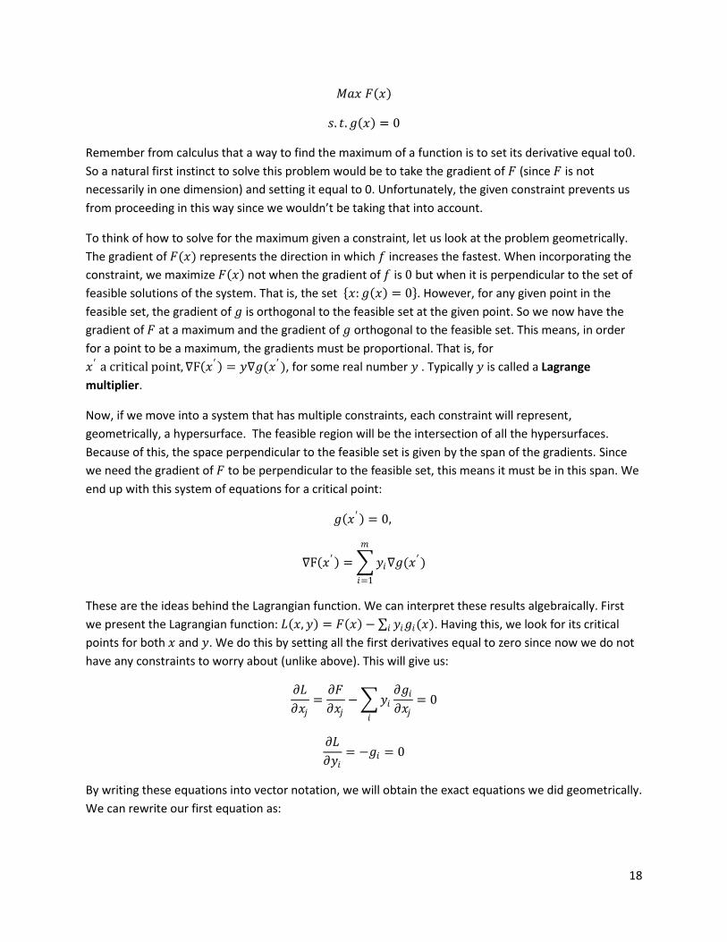
𝑀𝑎𝑥 𝐹 𝑥

𝑠. 𝑡. 𝑔 𝑥 = 0

Remember from calculus that a way to find the maximum of a function is to set its derivative equal to0.

So a natural first instinct to solve this problem would be to take the gradient of 𝐹 (since 𝐹 is not

necessarily in one dimension) and setting it equal to 0. Unfortunately, the given constraint prevents us

from proceeding in this way since we wouldn’t be taking that into account.

To think of how to solve for the maximum given a constraint, let us look at the problem geometrically.

The gradient of 𝐹(𝑥) represents the direction in which 𝑓 increases the fastest. When incorporating the

constraint, we maximize 𝐹 𝑥 not when the gradient of 𝑓 is 0 but when it is perpendicular to the set of

feasible solutions of the system. That is, the set 𝑥: 𝑔 𝑥 = 0 . However, for any given point in the

feasible set, the gradient of 𝑔 is orthogonal to the feasible set at the given point. So we now have the

gradient of 𝐹 at a maximum and the gradient of 𝑔 orthogonal to the feasible set. This means, in order

for a point to be a maximum, the gradients must be proportional. That is, for

𝑥′ a critical point, ∇F 𝑥′ = 𝑦∇𝑔(𝑥′), for some real number 𝑦 . Typically 𝑦 is called a Lagrange

multiplier.

Now, if we move into a system that has multiple constraints, each constraint will represent,

geometrically, a hypersurface. The feasible region will be the intersection of all the hypersurfaces.

Because of this, the space perpendicular to the feasible set is given by the span of the gradients. Since

we need the gradient of 𝐹 to be perpendicular to the feasible set, this means it must be in this span. We

end up with this system of equations for a critical point:

𝑔 𝑥′ = 0,

∇F 𝑥′ = 𝑦𝑖∇𝑔(𝑥 ′)

𝑚

𝑖=1

These are the ideas behind the Lagrangian function. We can interpret these results algebraically. First

we present the Lagrangian function: 𝐿 𝑥, 𝑦 = 𝐹 𝑥 − 𝑦𝑖𝑔𝑖(𝑥)𝑖 . Having this, we look for its critical

points for both 𝑥 and 𝑦. We do this by setting all the first derivatives equal to zero since now we do not

have any constraints to worry about (unlike above). This will give us:

𝜕𝐿

𝜕𝑥𝑗=

𝜕𝐹

𝜕𝑥𝑗− 𝑦𝑖

𝜕𝑔𝑖

𝜕𝑥𝑗𝑖

= 0

𝜕𝐿

𝜕𝑦𝑖= −𝑔𝑖 = 0

By writing these equations into vector notation, we will obtain the exact equations we did geometrically.

We can rewrite our first equation as:

19

𝜕𝐹

𝜕𝑥𝑗= 𝑦𝑖

𝜕𝑔𝑖

𝜕𝑥𝑗𝑖

In vector form, for the critical point, this is nothing else but ∇𝐹 𝑥′ = 𝑦𝑖∇𝑔(𝑥′)𝑚𝑖=1 , our first equation

we derived geometrically. It is even easier to see that −𝑔𝑖 = 0 is equivalent to 𝑔 𝑥′ = 0 for the critical

point. These equations we have introduced for the derivatives are typically called the first-order

optimality conditions.

It is possible to apply these ideas to the barrier function.

Given the general logarithmic barrier function for an LP: 𝑐𝑇𝑥 + 𝜇 log 𝑥𝑗𝑗 + 𝜇 log 𝑤𝑖𝑖

and having 𝐴𝑥 + 𝑤 = 𝑏 as the constraints, the Lagrangian is:

𝐿 𝑥, 𝑤, 𝑦 = 𝑐𝑇𝑥 + 𝜇 log 𝑥𝑗

𝑗

+ 𝜇 log 𝑤𝑖

𝑖

+ 𝑦𝑇(𝑏 − 𝐴𝑥 − 𝑤)

In general, the first-order optimality conditions will be:

𝜕𝐿

𝜕𝑥𝑗= 𝑐𝑗 + 𝜇

1

𝑥𝑗− 𝑦𝑗 𝑎𝑖𝑗 = 0, 𝑗 = 1,2, … . . , 𝑛

𝜕𝐿

𝜕𝑤𝑖= 𝜇

1

𝑤𝑖− 𝑦𝑖 = 0, 𝑖 = 1,2, … . . , 𝑚

𝜕𝐿

𝜕𝑦𝑖= 𝑏𝑖 − 𝑎𝑖𝑗 𝑥𝑗

𝑗

− 𝑤𝑖 = 0, 𝑖 = 1,2, … . 𝑚

In the case of our example, implementing the Lagrangian process is as follows:

𝐿𝑃 𝑥1 , 𝑥2, 𝑝, 𝑞 = 𝑥1 − 2𝑥2 + 𝜇 log 𝑥1 + 𝜇 log 𝑥2 + 𝜇 log 𝑝 + 𝜇 log 𝑞 + 𝑦1 1 + 𝑥2 − 𝑝 + 𝑦2(2 − 𝑥1 − 𝑞)

𝐿𝐷 𝑦1 , 𝑦2 , 𝑡1, 𝑡2 = −𝑦1 + 2𝑦2 + 𝜇 log 𝑦1 + 𝜇 log 𝑦2 + 𝜇 log 𝑡1 + 𝜇 log 𝑡2 + 𝑥1 1 − 𝑦2 + 𝑡2 + 𝑥2(−2 + 𝑦1 + 𝑡2)

Following through with the primal, the corresponding first derivatives are:

𝜕𝐿𝑃

𝜕𝑥1= 1 + 𝜇

1

𝑥1− 𝑦2

𝜕𝐿𝑃

𝜕𝑦2= −2 + 𝜇

1

𝑥2+ 𝑦1

𝜕𝐿𝑃

𝜕𝑝= 𝜇

1

𝑝− 𝑦1

𝜕𝐿𝑃

𝜕𝑞= 𝜇

1

𝑞− 𝑦2

𝜕𝐿𝑃

𝜕𝑥1= 1 + 𝑥2 − 𝑝

20

𝜕𝐿𝑃

𝜕𝑥2= 2 − 𝑥1 − 𝑞

These can be simplified into the above general format for the first-order optimality conditions.

We can rewrite these general equations for the first-order optimality conditions into matrix form. In this

form, 𝑋 and 𝑊 will be diagonal matrices whose diagonal entries are the components of the vector 𝑥 and

𝑤, respectively. The matrix form is shown below.

𝐴𝑇𝑦 − 𝜇𝑋−1𝑒 = 𝑐

𝑦 = 𝜇𝑊−1𝑒

𝐴𝑥 + 𝑤 = 𝑏

We introduce a vector 𝑧 = 𝜇𝑋−1𝑒, allowing us to rewrite this as

𝐴𝑥 + 𝑤 = 𝑏

𝐴𝑇𝑦 − 𝑧 = 𝑐

𝑧 = 𝜇𝑋−1𝑒

𝑦 = 𝜇𝑊−1𝑒

By multiplying the third equation through by 𝑋 and the fourth equation through by 𝑊, we will get a

primal-dual symmetric form for these equations [2]. In these equations, we introduce 𝑍 and 𝑌 which

have the same properties of 𝑋 and 𝑊. They are diagonal matrices whose diagonal entries are the

components of their respective vector. With these modifications, the equations are

𝐴𝑥 + 𝑤 = 𝑏

𝐴𝑇𝑦 − 𝑧 = 𝑐

𝑋𝑍𝑒 = 𝜇𝑒

𝑌𝑊𝑒 = 𝜇𝑒

The last two equations are called the µ-complementary conditions because if you let 𝜇 = 0 then they

are the usual complementary slackness conditions that need to be satisfied at optimality [2].

In the case of our example, once we write down the problem in terms of these newly developed

equations, we can use simple algebra and substitution to obtain a solution.

2.3.1.3 The Central Path and the Path-Following Method

When discussing the barrier problem and Lagrangians, we must first explore the idea of the central path.

When we introduced the logarithmic barrier function, we included a constant 𝜇 that scaled the

logarithm term. Remember we noticed that because the barrier function depends on µ, a whole set of

21

functions were created that were parameterized by µ. For each µ, we typically have a unique solution

which is obtained somewhere in the interior of the feasible region. As µ goes to zero, the barrier

function goes to the original objective function so, as we take smaller and smaller µ values and obtain

the corresponding solutions, we will move closer and closer to the optimal solution of the original

objective function. If all these solutions are plotted, one will notice a path is created through the feasible

region leading to the optimal solution. This path is called the central path.

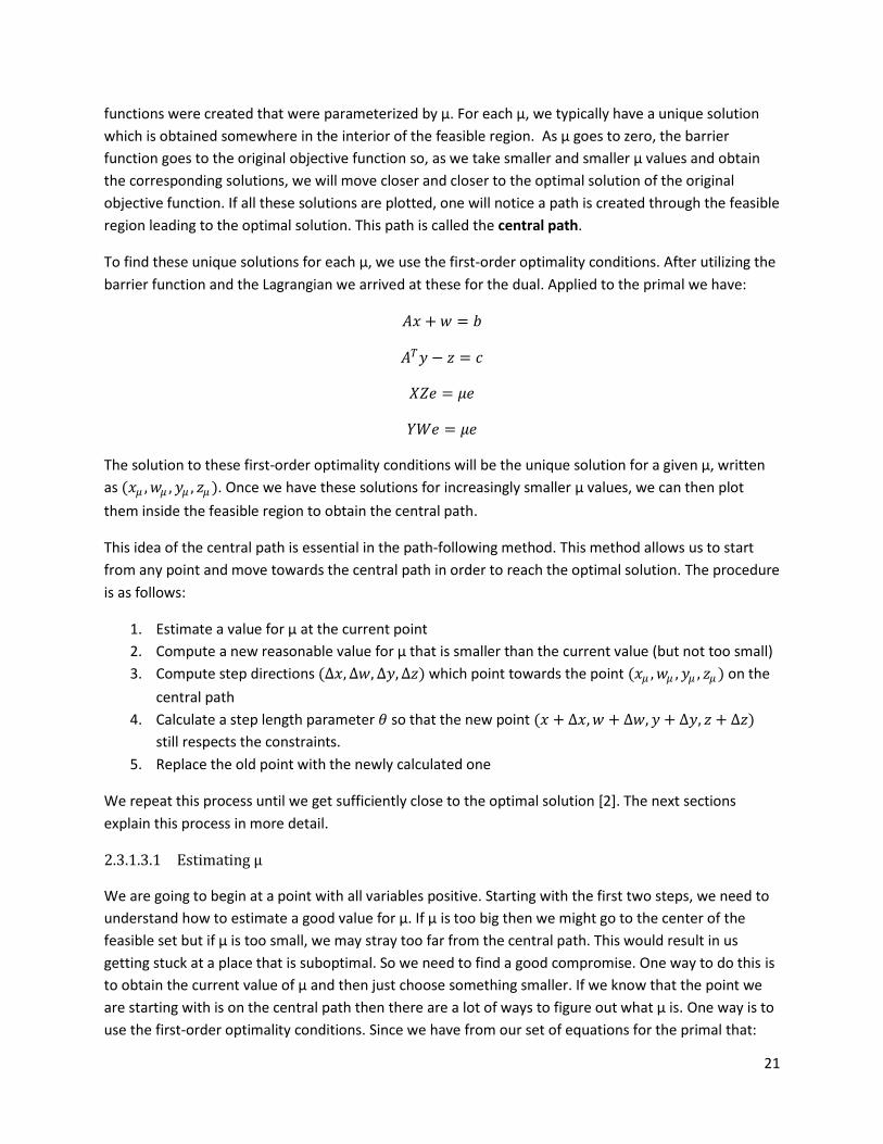
To find these unique solutions for each µ, we use the first-order optimality conditions. After utilizing the

barrier function and the Lagrangian we arrived at these for the dual. Applied to the primal we have:

𝐴𝑥 + 𝑤 = 𝑏

𝐴𝑇𝑦 − 𝑧 = 𝑐

𝑋𝑍𝑒 = 𝜇𝑒

𝑌𝑊𝑒 = 𝜇𝑒

The solution to these first-order optimality conditions will be the unique solution for a given µ, written

as (𝑥𝜇 , 𝑤𝜇 , 𝑦𝜇 , 𝑧𝜇 ). Once we have these solutions for increasingly smaller µ values, we can then plot

them inside the feasible region to obtain the central path.

This idea of the central path is essential in the path-following method. This method allows us to start

from any point and move towards the central path in order to reach the optimal solution. The procedure

is as follows:

1. Estimate a value for µ at the current point

2. Compute a new reasonable value for µ that is smaller than the current value (but not too small)

3. Compute step directions (∆𝑥, ∆𝑤, ∆𝑦, ∆𝑧) which point towards the point (𝑥𝜇 , 𝑤𝜇 , 𝑦𝜇 , 𝑧𝜇 ) on the

central path

4. Calculate a step length parameter 𝜃 so that the new point (𝑥 + ∆𝑥, 𝑤 + ∆𝑤, 𝑦 + ∆𝑦, 𝑧 + ∆𝑧)

still respects the constraints.

5. Replace the old point with the newly calculated one

We repeat this process until we get sufficiently close to the optimal solution [2]. The next sections

explain this process in more detail.

2.3.1.3.1 Estimating µ

We are going to begin at a point with all variables positive. Starting with the first two steps, we need to

understand how to estimate a good value for µ. If µ is too big then we might go to the center of the

feasible set but if µ is too small, we may stray too far from the central path. This would result in us

getting stuck at a place that is suboptimal. So we need to find a good compromise. One way to do this is

to obtain the current value of µ and then just choose something smaller. If we know that the point we

are starting with is on the central path then there are a lot of ways to figure out what µ is. One way is to

use the first-order optimality conditions. Since we have from our set of equations for the primal that:

22

𝑋𝑍𝑒 = 𝜇𝑒

𝑌𝑊𝑒 = 𝜇𝑒

we can solve these for µ and then average the values. Doing this will give us the following equation:

𝜇 =𝑧𝑇𝑥 + 𝑦𝑡𝑤

𝑛 + 𝑚

If we know that our starting point is definitely on the path, we can use this equation to get the exact

value for µ. However, we can still use it find 𝜇 when the point is not on the central path. It will just be an

estimate. Since we are trying to get closer to optimality and we know this occurs as µ gets smaller, we

need a µ that is smaller than the current value. So we take the above equation and multiply it by a

fraction. Let this fraction be represented by δ. So for any point we can estimate our new µ value by:

𝜇 = 𝛿𝑧𝑇𝑥 + 𝑦𝑡𝑤

𝑛 + 𝑚

2.3.1.3.2 Step Directions and Newton’s Method

Now as we move on to step three, we need to understand how we compute a step direction. First,

though, we must discuss Newton’s method. Newton’s method allows one to find the point where a

given function equals zero using differentiability and smoothness properties. It solves this problem as

follows: given any point, find a step direction such that if we go in that direction and find a new point,

the function evaluated at that new point will be close to zero. Ideally, given a function 𝐹(𝑥) and a point

𝑝, we want to find a direction ∆𝑝 such that 𝐹 𝑝 + ∆𝑝 = 0. This method works well when the function is

linear, however, if it is nonlinear, it is not possible to solve. To accommodate this, if given a nonlinear

function, we implement the Taylor series and use the first two terms to approximate the function. So we

have:

𝐹 𝑝 + ∆𝑝 ≈ 𝐹 𝑝 + 𝐹′ (𝑝)∆𝑝

This can also be applied to a set of functions where:

𝐹 𝑝 =

𝐹1(𝑝)𝐹2(𝑝)

⋮𝐹𝑁(𝑝)

, 𝑝 =

𝑝1

𝑝2

⋮𝑝𝑁

𝑎𝑛𝑑 𝐹′ 𝑝 =

𝜕𝐹1

𝜕𝑝1⋯

𝜕𝐹1

𝜕𝑝𝑁

⋮ ⋱ ⋮𝜕𝐹𝑁

𝜕𝑝1⋯

𝜕𝐹𝑁

𝜕𝑝𝑁

Setting the function equal to zero, we will obtain the following equation and are then able to solve for

∆𝑝:

𝐹′ 𝑝 ∆𝑝 = −𝐹(𝑝)

Once we know ∆𝑝 we can then change our current point to 𝑝 + ∆𝑝 and evaluate the function at the new

point. This process repeats until the value of the function gets approximately equal to 0.

23

That is the process of Newton’s method and it will be a guide for how we proceed to find the step

direction. We want to find a direction such that if we move in that direction, the new point we end up at

will be on the central path. Remember that on the central path, for the primal, we have the following

first-order optimality conditions:

𝐴𝑥 + 𝑤 = 𝑏

𝐴𝑇𝑦 − 𝑧 = 𝑐

𝑋𝑍𝑒 = 𝜇𝑒

𝑌𝑊𝑒 = 𝜇𝑒

So if our new point is on the central path we should have the following:

𝐴 𝑥 + ∆𝑥 + (𝑤 + ∆𝑤) = 𝑏

𝐴𝑇(𝑦 + ∆𝑦) − (𝑧 + ∆𝑧) = 𝑐

𝑋 + ∆𝑋 (𝑍 + ∆𝑍)𝑒 = 𝜇𝑒

𝑌 + ∆𝑌 (𝑊 + ∆𝑊)𝑒 = 𝜇𝑒

We rewrite these equations with all the unknowns on one side and the knowns on the other. Our

current point is (𝑥, 𝑤, 𝑦, 𝑧), so we know these values. This leaves us with:

𝐴∆𝑥 + ∆𝑤 = 𝑏 − 𝐴𝑥 − 𝑤

𝐴𝑇∆𝑦 − ∆𝑧 = 𝑐 − 𝐴𝑇𝑦 + 𝑧

𝑍∆𝑥 + 𝑋∆𝑧 + ∆𝑋∆𝑍𝑒 = 𝜇𝑒 − 𝑋𝑍𝑒

𝑊∆𝑦 + 𝑌∆𝑤 + ∆𝑌∆𝑊𝑒 = 𝜇𝑒 − 𝑌𝑊𝑒

If we let 𝜌 = 𝑏 − 𝐴𝑥 − 𝑤 and 𝜍 = 𝑐 − 𝐴𝑇𝑦 + 𝑧, we can simplify the equations. Also, we want to have a

linear system. In order to do this, we drop the nonlinear terms. (It may be surprising that we can do this

but it is just a result of Newton’s method. As ∆𝑋 and ∆𝑍 get negligible, which occurs when we utilize

Newton’s method, their product goes to zero even faster, making the term ∆𝑋∆𝑍𝑒 become irrelevant.

Similarly this happens for ∆𝑌 and ∆𝑊 in the last equation.)

Modifying the equations as such, we end up with

𝐴∆𝑥 + ∆𝑤 = 𝜌

𝐴𝑇∆𝑦 − ∆𝑧 = 𝜍

𝑍∆𝑥 + 𝑋∆𝑧 = 𝜇𝑒 − 𝑋𝑍𝑒

𝑊∆𝑦 + 𝑌∆𝑤 = 𝜇𝑒 − 𝑌𝑊𝑒

24

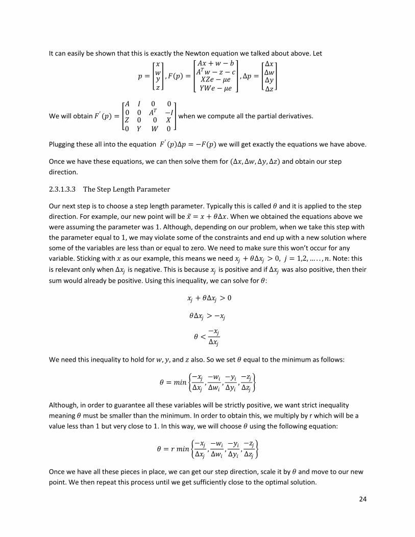
It can easily be shown that this is exactly the Newton equation we talked about above. Let

𝑝 =

𝑥𝑤𝑦𝑧

, 𝐹 𝑝 =

𝐴𝑥 + 𝑤 − 𝑏𝐴𝑇𝑤 − 𝑧 − 𝑐𝑋𝑍𝑒 − 𝜇𝑒𝑌𝑊𝑒 − 𝜇𝑒

, ∆𝑝 =

∆𝑥∆𝑤∆𝑦∆𝑧

We will obtain 𝐹′(𝑝) =

𝐴 𝐼0 0

0 0𝐴𝑇 −𝐼

𝑍 00 𝑌

0 𝑋𝑊 0

when we compute all the partial derivatives.

Plugging these all into the equation 𝐹′ 𝑝 ∆𝑝 = −𝐹(𝑝) we will get exactly the equations we have above.

Once we have these equations, we can then solve them for (∆𝑥, ∆𝑤, ∆𝑦, ∆𝑧) and obtain our step

direction.

2.3.1.3.3 The Step Length Parameter

Our next step is to choose a step length parameter. Typically this is called 𝜃 and it is applied to the step

direction. For example, our new point will be �� = 𝑥 + 𝜃∆𝑥. When we obtained the equations above we

were assuming the parameter was 1. Although, depending on our problem, when we take this step with

the parameter equal to 1, we may violate some of the constraints and end up with a new solution where

some of the variables are less than or equal to zero. We need to make sure this won’t occur for any

variable. Sticking with 𝑥 as our example, this means we need 𝑥𝑗 + 𝜃∆𝑥𝑗 > 0, 𝑗 = 1,2, … . . , 𝑛. Note: this

is relevant only when ∆𝑥𝑗 is negative. This is because 𝑥𝑗 is positive and if ∆𝑥𝑗 was also positive, then their

sum would already be positive. Using this inequality, we can solve for 𝜃:

𝑥𝑗 + 𝜃∆𝑥𝑗 > 0

𝜃∆𝑥𝑗 > −𝑥𝑗

𝜃 <−𝑥𝑗

∆𝑥𝑗

We need this inequality to hold for 𝑤, 𝑦, and 𝑧 also. So we set 𝜃 equal to the minimum as follows:

𝜃 = 𝑚𝑖𝑛 −𝑥𝑗

∆𝑥𝑗,−𝑤𝑖

∆𝑤𝑖,−𝑦𝑖

∆𝑦𝑖,−𝑧𝑗

∆𝑧𝑗

Although, in order to guarantee all these variables will be strictly positive, we want strict inequality

meaning 𝜃 must be smaller than the minimum. In order to obtain this, we multiply by r which will be a

value less than 1 but very close to 1. In this way, we will choose 𝜃 using the following equation:

𝜃 = 𝑟 𝑚𝑖𝑛 −𝑥𝑗

∆𝑥𝑗,−𝑤𝑖

∆𝑤𝑖,−𝑦𝑖

∆𝑦𝑖,−𝑧𝑗

∆𝑧𝑗

Once we have all these pieces in place, we can get our step direction, scale it by 𝜃 and move to our new

point. We then repeat this process until we get sufficiently close to the optimal solution.

25

2.3.2 Interior Point Method for Semidefinite Programming

The ideas just presented are adapted to semidefinite programming in the paper of Christoph Helmberg,

Franz Rendl, Robert Vanderbei, and Henry Wolkowicz, An Interior Point Method for Semidefinite

Programming [1]. They propose an interior point method algorithm for optimization problems over

semidefinite matrices. Their algorithm follows closely to the path following method with necessary

adaptations to semidefinite programming. The algorithm is described in this section.

Helmberg et al. work with the following primal and dual semidefinite problems [1]:

(Primal) 𝑀𝑎𝑥 𝑇𝑟 (𝐶𝑋)

s.t. 𝑎 − 𝐴 𝑥 = 0

𝑏 − 𝐵 𝑥 ≥ 0

𝑋 ≽ 0

(Dual) 𝑀𝑖𝑛 𝑎𝑇𝑦 + 𝑏𝑇𝑡

s.t. 𝐴𝑇 𝑦 + 𝐵𝑇 𝑡 − 𝐶 ≽ 0

𝑦𝜖𝑅𝑘 , 𝑡𝜖𝑅+𝑚

We can apply our original example, introduced in the last section, to this notation as such:

If we denote 𝐶 = 1 00 −2

and 𝑋 = 𝑥1 00 𝑥2

,

the objective function of the primal can be written as 𝑇𝑟 (𝐶𝑋) = 𝑥1 − 2𝑥2

If we let 𝑏 = −12

,

the inequality constraints can be written as 𝑏 − 𝐵 𝑥 = −1 + 𝑥2

2 − 𝑥1

which is greater than or equal to 00 since we need 𝑥2 ≥ 1and 𝑥1 ≤ 2.

So we can rewrite the primal in this format as:

𝑀𝑎𝑥 𝑇𝑟 (𝐶𝑋)

s.t. 𝑏 − 𝐵 𝑥 ≥ 0

𝑋 ≽ 0

26

Similar to the way we constructed the inequality constraints, we can construct equality constraints if

they were included in the problem. This would result in adding a term 𝑎 − 𝐴 𝑥 = 0 (In our case, we do

not have any equality constraints so we would not include this).

We can do the same for the dual:

𝑡 = 𝑦1𝑦2

, 𝑏 = −12

making 𝑏𝑇𝑡 = −1 2 𝑦1𝑦2

= −𝑦1 + 2𝑦2 (𝑎𝑇𝑦 does not appear in this case)

𝐶 = 1 00 −2

so 𝐵𝑇 𝑡 − 𝐶 = 𝑦2 − 1 0

0 −𝑦1 + 2 ≽ 0 since it is symmetric and the diagonal entries

are greater than zero. This will give us the dual problem as:

𝑀𝑖𝑛 𝑎𝑇𝑦 + 𝑏𝑇𝑡

s.t. 𝐵𝑇 𝑡 − 𝐶 ≽ 0

𝑦𝜖𝑅𝑘 , 𝑡𝜖𝑅+𝑚

Similarly, if equality constraints were included in the system, we would have to take those into account

when converting to the dual. This would result in a term being added in the objective function

(𝑎𝑇𝑦) and a term being added in the inequality constraint (𝐴𝑇 𝑦 ). Since we do not have any equality

constraints, these are not included above.

This construction of the primal and dual system is the same used by Helmberg et al. They begin their

algorithm by defining their system as stated previously and again here:

(Primal) 𝑀𝑎𝑥 𝑇𝑟 (𝐶𝑋)

s.t. 𝑎 − 𝐴 𝑋 = 0

𝑏 − 𝐵 𝑋 ≥ 0

𝑋 ≽ 0

(Dual) 𝑀𝑖𝑛 𝑎𝑇𝑦 + 𝑏𝑇𝑡

s.t. 𝐴𝑇 𝑦 + 𝐵𝑇 𝑡 − 𝐶 ≽ 0

𝑦𝜖𝑅𝑘 , 𝑡𝜖𝑅+𝑚

For their algorithm they require a matrix 𝑋 that strictly satisfies the above inequalities

(𝑖. 𝑒. 𝑏 − 𝐵 𝑋 ≥ 0) and is positive definite (that is it is symmetric and all of its eigenvalues are

positive). Also they assume that the equality constraints on 𝑋 are linearly independent (if not, we could

simply row reduce the linear system).

27

At first, the linear operators, 𝐴 and 𝐵, were defined for symmetric matrices. However, it is realized that

they will have to be applied to non-symmetric matrices. This problem is resolved by writing a matrix, 𝑀,

in terms of its symmetric and non-symmetric parts:

𝑀 = 𝑠𝑦𝑚𝑚𝑒𝑡𝑟𝑖𝑐 + 𝑠𝑘𝑒𝑤 =1

2 𝑀 + 𝑀𝑇 +

1

2(𝑀 − 𝑀𝑇)

and then letting the skew, or non-symmetric, part map to 0. Observe:

1

2 𝑀 − 𝑀𝑇 = 0 → 𝑀 = 𝑀𝑇

In this way, when we apply 𝐴 or 𝐵 to the non-symmetric matrix 𝑀, we have the definition that

𝐴 𝑀 = 𝐴 𝑀𝑇 (𝑠𝑖𝑚𝑖𝑙𝑎𝑟𝑙𝑦 𝐵 𝑀 = 𝐵 𝑀𝑇 ).

Now taking the system with all adjustments above integrated, we rewrite it into equality form

introducing 𝑍 as a slack variable. Applying the ideas of the barrier problem to the dual system we have:

𝑀𝑖𝑛 𝑎𝑇𝑦 + 𝑏𝑇𝑡 − 𝜇 log 𝑑𝑒𝑡𝑍 + 𝑒𝑇 log 𝑡

𝑠. 𝑡. 𝐴𝑇 𝑦 + 𝐵𝑇 𝑡 − 𝐶 = 𝑍

𝑡 ≥ 0, 𝑍 ≽ 0

Now we formulate the Lagrangian of this barrier function:

𝐿𝜇 𝑋, 𝑦, 𝑡, 𝑍 = 𝑎𝑇𝑦 + 𝑏𝑇𝑡 − 𝜇 log 𝑑𝑒𝑡𝑍 + 𝑒𝑇 log 𝑡 + 𝑍 + 𝐶 − 𝐴𝑇 𝑦 − 𝐵𝑇 𝑡 , 𝑋

Before taking the gradient to obtain the first-order derivatives, we will introduce the adjoint identity

presented by Helmberg et al.:

𝐴 𝑋 , 𝑦 = 𝑋, 𝐴𝑇(𝑦)

Utilizing this property we can write out the last expression in the Lagrangian as:

𝑍 + 𝐶 − 𝐴𝑇 𝑦 − 𝐵𝑇 𝑡 , 𝑋 = 𝑍, 𝑋 + 𝐶, 𝑋 − 𝐴 𝑋 , 𝑦 − 𝐵 𝑋 , 𝑡 .

With these modifications, our Lagrangian is now:

𝐿𝜇 𝑋, 𝑦, 𝑡, 𝑍 = 𝑎𝑇𝑦 + 𝑏𝑇𝑡 − 𝜇 log 𝑑𝑒𝑡𝑍 + 𝑒𝑇 log 𝑡 + 𝑍, 𝑋 + 𝐶, 𝑋 − 𝐴 𝑋 , 𝑦 − 𝐵 𝑋 , 𝑡 .

Now, taking the partial derivatives with this adjustment above, we end up with the following first-order

optimality conditions:

∇𝑋𝐿𝜇 = 𝑍 + 𝐶 − 𝐴𝑇 𝑦 − 𝐵𝑇 𝑡 = 0

∇𝑦𝐿𝜇 = 𝑎 − 𝐴 𝑋 = 0

∇𝑡𝐿𝜇 = 𝑏 − 𝐵 𝑋 − 𝜇𝑡−1 = 0

28

∇𝑍𝐿𝜇 = 𝑋 − 𝜇𝑍−1 = 0

Using the last two equations, we can derive an equation for the µ value associated with a given point on

the central trajectory, similar to what we did previously in the path following method. Our goal is to

extend these properties in a reasonable way to get a 𝜇 value for solutions not on the central path. We

start by solving the first and second equations for µ:

𝑏 − 𝐵 𝑋 = 𝜇𝑡−1 → 𝑑𝑖𝑣𝑖𝑑𝑒 𝑡𝑕𝑟𝑜𝑢𝑔𝑕 𝑏𝑦 𝑡−1 → 𝜇 = 𝑡𝑇(𝑏 − 𝐵 𝑋 )

𝑋 = 𝜇𝑍−1 → 𝑑𝑖𝑣𝑖𝑑𝑒 𝑡𝑕𝑟𝑜𝑢𝑔𝑕 𝑏𝑦 𝑍−1 → 𝜇 = 𝑡𝑟(𝑍𝑋)

We average the two equations by adding the equations together and dividing by the sum of the

corresponding lengths to arrive at:

𝜇 =𝑡𝑟 𝑍𝑋 + 𝑡𝑇(𝑏 − 𝐵 𝑋 )

𝑛 + 𝑚

The algorithm being presented by Helmberg et al. proceeds from here in a fashion similar to that of the

point-following method. It takes a point (𝑋, 𝑦, 𝑡, 𝑍) where 𝑋, 𝑍 ≻ 0, 𝑡 ≥ 0, 𝑎𝑛𝑑 𝑏 − 𝐵(𝑥) > 0. Then

using the above equation for µ, estimates the current value for µ and divides it by 2. Dividing by 2 will

guarantee that the new µ will be less than the current value of µ. The algorithm next computes

directions (∆𝑋, ∆𝑦, ∆𝑡, ∆𝑍) such that when applied to the original point, the new point, (𝑋 + ∆𝑋, 𝑦 +

∆𝑦, 𝑡 + ∆𝑡, 𝑍 + ∆𝑍), is on the central path at the determined µ.

Remember from the discussion of the path following method, the way to find the new point was to

solve the first-order optimality conditions for the step direction. Again, not all the first-order optimality

conditions are linear so we are unable to solve the system directly. We must rewrite the last two

equations (which are the two that are nonlinear) by applying a linearization. To do this, we find the

linear approximations to our nonlinear functions and utilize those to solve our system. Many choices

could be made for our linearization. Helmberg et al. list these seven possibilities [1]:

𝜇𝐼 − 𝑍1/2𝑋𝑍1/2 = 0

𝜇𝐼 − 𝑋1/2𝑍𝑋1/2 = 0

𝜇𝑍−1 − 𝑋 = 0

𝜇𝑋−1 − 𝑍 = 0

𝑍𝑋 − 𝜇𝐼 = 0

𝑋𝑍 − 𝜇𝐼 = 0

𝑍𝑋 + 𝑋𝑍 − 2𝜇𝐼 = 0

The first two, in semidefinite programming, involve matrix square roots making them not very good

choices computationally. The third doesn’t contain any information about the primal variables and the

29

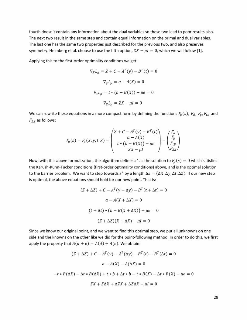
fourth doesn’t contain any information about the dual variables so these two lead to poor results also.

The next two result in the same step and contain equal information on the primal and dual variables.

The last one has the same two properties just described for the previous two, and also preserves

symmetry. Helmberg et al. choose to use the fifth option, 𝑍𝑋 − 𝜇𝐼 = 0, which we will follow [1].

Applying this to the first-order optimality conditions we get:

∇𝑋𝐿𝜇 = 𝑍 + 𝐶 − 𝐴𝑇 𝑦 − 𝐵𝑇 𝑡 = 0

∇𝑦𝐿𝜇 = 𝑎 − 𝐴 𝑋 = 0

∇𝑡𝐿𝜇 = 𝑡 ∘ (𝑏 − 𝐵 𝑋 ) − 𝜇𝑒 = 0

∇𝑍𝐿𝜇 = 𝑍𝑋 − 𝜇𝐼 = 0

We can rewrite these equations in a more compact form by defining the functions 𝐹𝜇 𝑠 , 𝐹𝑑 , 𝐹𝑝 , 𝐹𝑡𝐵 and

𝐹𝑍𝑋 as follows:

𝐹𝜇 𝑠 = 𝐹𝜇 𝑋, 𝑦, 𝑡, 𝑍 =

𝑍 + 𝐶 − 𝐴𝑇 𝑦 − 𝐵𝑇 𝑡

𝑎 − 𝐴 𝑋

𝑡 ∘ 𝑏 − 𝐵 𝑋 − 𝜇𝑒

𝑍𝑋 − 𝜇𝐼

=

𝐹𝑑

𝐹𝑝

𝐹𝑡𝐵

𝐹𝑍𝑋

Now, with this above formulization, the algorithm defines 𝑠∗ as the solution to 𝐹𝜇 𝑠 = 0 which satisfies

the Karush-Kuhn-Tucker conditions (first-order optimality conditions) above, and is the optimal solution

to the barrier problem. We want to step towards 𝑠∗ by a length ∆𝑠 = ∆𝑋, ∆𝑦, ∆𝑡, ∆𝑍 . If our new step

is optimal, the above equations should hold for our new point. That is:

𝑍 + ∆𝑍 + 𝐶 − 𝐴𝑇 𝑦 + ∆𝑦 − 𝐵𝑇 𝑡 + ∆𝑡 = 0

𝑎 − 𝐴 𝑋 + ∆𝑋 = 0

𝑡 + ∆𝑡 ∘ 𝑏 − 𝐵 𝑋 + ∆𝑋 − 𝜇𝑒 = 0

𝑍 + ∆𝑍 𝑋 + ∆𝑋 − 𝜇𝐼 = 0

Since we know our original point, and we want to find this optimal step, we put all unknowns on one

side and the knowns on the other like we did for the point-following method. In order to do this, we first

apply the property that 𝐴 𝑑 + 𝑒 = 𝐴 𝑑 + 𝐴(𝑒). We obtain:

𝑍 + ∆𝑍 + 𝐶 − 𝐴𝑇 𝑦) − 𝐴𝑇(∆𝑦 − 𝐵𝑇 𝑡) − 𝐵𝑇(∆𝑡 = 0

𝑎 − 𝐴 𝑋) − 𝐴(∆𝑋 = 0

−𝑡 ∘ 𝐵 ∆𝑋 − ∆𝑡 ∘ 𝐵 ∆𝑋 + 𝑡 ∘ 𝑏 + ∆𝑡 ∘ 𝑏 − 𝑡 ∘ 𝐵 𝑋 − ∆𝑡 ∘ 𝐵 𝑋 − 𝜇𝑒 = 0

𝑍𝑋 + 𝑍∆𝑋 + ∆𝑍𝑋 + ∆𝑍∆𝑋 − 𝜇𝐼 = 0

30

We replace the last entry by 𝑍𝑋 + 𝑍∆𝑋 + ∆𝑍𝑋 − 𝜇𝐼 by using the ideas of Taylor’s approximation: As ∆𝑋

and ∆𝑍 become negligible, their product goes to zero even faster. We can do similarly for the third

equation by getting rid of the ∆𝑡 ∘ 𝐵 ∆𝑋 term.

Now by putting the knowns and unknowns onto separate sides we have:

∆𝑍 − 𝐴𝑇 ∆𝑦 − 𝐵𝑇 ∆𝑡 = −𝑍 − 𝐶 + 𝐴𝑇 𝑦 + 𝐵𝑇 𝑡

−𝐴 ∆𝑋 = −𝑎 + 𝐴 𝑋

−𝑡 ∘ 𝐵 ∆𝑋 + ∆𝑡 ∘ 𝑏 − ∆𝑡 ∘ 𝐵 ∆𝑋 = −𝑡 ∘ 𝑏 + 𝑡 ∘ 𝐵 𝑋 + 𝜇𝑒

𝑍∆𝑋 + ∆𝑍𝑋 = −𝑍𝑋 + 𝜇𝐼

Simplified this is:

∆𝑍 − 𝐴𝑇 ∆𝑦 − 𝐵𝑇 ∆𝑡 = −𝑍 − 𝐶 + 𝐴𝑇 𝑦 + 𝐵𝑇 𝑡

−𝐴 ∆𝑋 = −𝑎 + 𝐴 𝑋

−𝑡 ∘ 𝐵 ∆𝑋 + ∆𝑡 ∘ 𝑏 − 𝐵 𝑋 = −𝑡 ∘ (𝑏 − 𝐵 𝑋 ) + 𝜇𝑒

𝑍∆𝑋 + ∆𝑍𝑋 = −𝑍𝑋 + 𝜇𝐼

Notice from the definitions above:

−𝑍 − 𝐶 + 𝐴𝑇 𝑦 + 𝐵𝑇 𝑡 = −𝐹𝑑

−𝑎 + 𝐴 𝑋 = −𝐹𝑝

−𝑡 ∘ 𝑏 − 𝐵 𝑋 + 𝜇𝑒 = −𝐹𝑡𝐵

−𝑍𝑋 + 𝜇𝐼 = −𝐹𝑍𝑋

We can rewrite these equations in the form of a matrix to show the system equals −𝐹𝜇 :

∆𝑍 − 𝐴𝑇(∆𝑦) − 𝐵𝑇(∆𝑡)−𝐴(∆𝑋)

−𝑡 ∘ 𝐵 ∆𝑋 + ∆𝑡 ∘ (𝑏 − 𝐵 𝑋 )𝑍∆𝑋 + ∆𝑍𝑋

= −

𝐹𝑑

𝐹𝑝

𝐹𝑡𝐵

𝐹𝑍𝑋

= −𝐹𝜇

Notice that this is simply the equation for Newton’s Method. We arrived at this same conclusion

previously for a general case when trying to understand how to find a step direction. In order to get a

step direction ∆𝑠 = ∆𝑋, ∆𝑦, ∆𝑡, ∆𝑍 towards 𝑠∗, we solve the equation

𝐹𝜇 + ∇𝐹𝜇 ∆𝑠 = 0 → ∇𝐹𝜇 ∆𝑠 = −𝐹𝜇 for ∆𝑠.

So now that we have these equations for the step direction set up, the next step is to actually obtain it.

We can begin by solving the first equation for ∆𝑍. We will arrive at:

31

∆𝑍 = −𝐹𝑑 + 𝐴𝑇 ∆𝑦 + 𝐵𝑇(∆𝑡)

Now that we have an expression for ∆𝑍 we can plug this into the last equation to obtain an expression

for ∆𝑋:

𝑍∆𝑋 + −𝐹𝑑 + 𝐴𝑇 ∆𝑦 + 𝐵𝑇 ∆𝑡 𝑋 = −𝐹𝑍𝑋

Expanding, we obtain:

𝑍∆𝑋 − 𝐹𝑑𝑋 + 𝐴𝑇 ∆𝑦 𝑋 + 𝐵𝑇 ∆𝑡 𝑋 = −𝐹𝑍𝑋

and bringing everything without a ∆𝑋 to the other side:

𝑍∆𝑋 = −𝐹𝑍𝑋 + 𝐹𝑑𝑋 − 𝐴𝑇 ∆𝑦 𝑋 − 𝐵𝑇 ∆𝑡 𝑋

Multiply through by 𝑍−1; since 𝑍 is a diagonal matrix with strictly positive entries on the

diagonal, we may write:

∆𝑋 = −𝑍−1𝐹𝑍𝑋 + 𝑍−1𝐹𝑑𝑋 − 𝑍−1𝐴𝑇 ∆𝑦 𝑋 − 𝑍−1𝐵𝑇 ∆𝑡 𝑋.

Simplifying and grouping terms together:

∆𝑋 = −𝑍−1𝐹𝑍𝑋 + 𝑍−1𝐹𝑑𝑋 − 𝑍−1(𝐴𝑇 ∆𝑦 + 𝐵𝑇 ∆𝑡 )𝑋

From the original equations, we had that 𝑍𝑋 − 𝜇𝐼 = 𝐹𝑍𝑋 . If we multiply this through by 𝑍−1 we

obtain 𝑋 − 𝜇𝐼𝑍−1 = 𝑍−1𝐹𝑍𝑋 . By plugging this in to our above equation for ∆𝑋, we arrive at:

∆𝑋 = 𝜇𝑍−1 − 𝑋 + 𝑍−1𝐹𝑑𝑋 − 𝑍−1(𝐴𝑇 ∆𝑦 + 𝐵𝑇 ∆𝑡 )𝑋

This is our equation for ∆𝑋.

Now if we plug this into the second first-order optimality condition, we can get an expression for ∆𝑦 and

∆𝑡:

−𝐴 𝜇𝑍−1 − 𝑋 + 𝑍−1𝐹𝑑𝑋 − 𝑍−1 𝐴𝑇 ∆𝑦 + 𝐵𝑇 ∆𝑡 𝑋 = −𝐹𝑝

Expanding this and dropping the negative:

𝐴 𝑍−1𝜇 − 𝐴 𝑋 + 𝐴 𝑍−1𝐹𝑑𝑋 − 𝐴 𝑍−1𝐴𝑇 ∆𝑦 𝑋 − 𝐴 𝑍−1𝐵𝑇 ∆𝑡 𝑋 = 𝐹𝑝

Remember that −𝐹𝑝 = −𝑎 + 𝐴(𝑋) so if we apply this we get:

𝐴 𝑍−1𝜇 − 𝐴 𝑋 + 𝐴 𝑍−1𝐹𝑑𝑋 − 𝐴 𝑍−1𝐴𝑇 ∆𝑦 𝑋 − 𝐴 𝑍−1𝐵𝑇 ∆𝑡 𝑋 = 𝑎 − 𝐴(𝑋)

The two 𝐴 𝑋 expressions cancel and by rearranging terms we arrive at:

𝐴 𝑍−1𝜇 + 𝐴 𝑍−1𝐹𝑑𝑋 − 𝑎 = 𝐴 𝑍−1𝐴𝑇 ∆𝑦 𝑋 + 𝐴 𝑍−1𝐵𝑇 ∆𝑡 𝑋

32

At this point, the authors introduce two linear operators, 𝑂11 and 𝑂12, and a vector 𝑣1 , defined as

follows:

𝑂11 ∙ = 𝐴(𝑍−1𝐴𝑇 ∙ 𝑋)

𝑂12 ∙ = 𝐴(𝑍−1𝐵𝑇 ∙ 𝑋)

𝑣1 = 𝐴 𝑍−1𝜇 + 𝐴 𝑍−1𝐹𝑑𝑋 − 𝑎

This is done so that the expression for ∆𝑦 and ∆𝑡 can be written more compactly. By applying the above

definitions to our equation we obtain this expression for ∆𝑦 and ∆𝑡:

𝑂11 ∆𝑦 + 𝑂12 ∆𝑡 = 𝑣1

We can also substitute our expression for ∆𝑋 into our third equation for the step direction to obtain

another expression for ∆𝑦 and ∆𝑡. In this case, two more operators, 𝑂21 and 𝑂22, and another vector,

𝑣2, are introduced. They are defined as:

𝑂21 ∙ = 𝐵(𝑍−1𝐴𝑇 ∙ 𝑋)

𝑂22 ∙ = 𝑏 − 𝐵 𝑋 ∘ 𝑡−1 ∘ ∙ + 𝐵(𝑍−1𝐵𝑇 ∙ 𝑋)

𝑣2 = 𝜇𝑡−1 − 𝑏 + 𝜇𝐵 𝑍−1) + 𝐵(𝑍−1𝐹𝑑𝑋

and allow us to write this expression for ∆𝑦 and ∆𝑡 as:

𝑂21 ∆𝑦 + 𝑂22 ∆𝑡 = 𝑣2

Now that we have all the equations for our steps, we can begin to solve them. Notice that the

expressions for ∆𝑦 and ∆𝑡 are all written in terms of things we know. So we first solve these for ∆𝑦

and ∆𝑡. Then once we have those values, we can plug them into our equation for ∆𝑍. Finally, once we

have the value for ∆𝑍, we can put all of these values into our expression for ∆𝑋 and solve. At this point,

we finally have obtained our step direction.

We note, however, that when we solve for ∆𝑋 we will not necessarily obtain a symmetric matrix. For

this reason, we will only use its symmetric part. We do this by remembering that a matrix can be written

in terms of its symmetric part plus its skew part like below:

𝑀 = 𝑠𝑦𝑚𝑚𝑒𝑡𝑟𝑖𝑐 + 𝑠𝑘𝑒𝑤 =1

2 𝑀 + 𝑀𝑇 +

1

2(𝑀 − 𝑀𝑇)

So by applying this to ∆𝑋 we have:

∆𝑋 =1

2 ∆𝑋 + ∆𝑋𝑇 +

1

2(∆𝑋 − ∆𝑋𝑇)

To use just the symmetric part, we say that ∆𝑋 =1

2 ∆𝑋 + ∆𝑋𝑇 with ∆𝑋 just denoting the new value we

will have for our step direction.

33

We now have our step direction ∆𝑠 = ∆𝑋, ∆𝑦, ∆𝑡, ∆𝑍 , but as previously noted in our discussion of the

path following method, we cannot automatically use this to step to our new point because we may

violate some constraints. In this case, we may violate the condition that 𝑡 and 𝑏 − 𝐵(𝑋) has to be

nonnegative and that 𝑋 and 𝑍 have to be positive definite. So we need to find a step length parameter

such that these conditions hold. Helmberg et al. do this by implementing a line search to get the

parameters 𝛼𝑝 and 𝛼𝑑 [1]. This process finds the minimum value of the objective function in one

dimension [4].

Once we have the step length parameters, we can step to our new point which will be:

𝑋 + 𝛼𝑝∆𝑋,

𝑦 + 𝛼𝑑∆𝑦,

𝑡 + 𝛼𝑑∆𝑡,

𝑍 + 𝛼𝑑∆𝑍

This process repeats until we obtain a point that satisfies the primal and dual feasibility and that gives a

sufficiently small duality gap. Until then, we update µ according to our new point and continue the

process to obtain our step directions and step length parameters.

Returning to our expressions we derived for ∆𝑦 and ∆𝑡, it can be shown that these equations can be

condensed into a system that is positive definite. Helmberg et al. present this and we will explore it

here.

Recall the definition of an adjoint linear operator:

𝐴 𝑋 , 𝑦 = 𝑋, 𝐴𝑇(𝑦)

Now we can see that 𝑂11 and 𝑂22 are self-adjoint and that 𝑂21 is the adjoint of 𝑂12. Helmberg et al. go

on further to state that our two new equations for ∆𝑦 and ∆𝑡 become a system of symmetric linear

equations and this system is positive definite [1]. We can show this by first defining a new operator. We

will call it 𝑂 and is defined as follows:

𝑂 𝑋 = 𝐴(𝑋)𝐵(𝑋)

Now using the adjoint definition from above, we can figure out what the adjoint of 𝑂 is.

𝑂 𝑋 , 𝑦𝑡 =

𝐴(𝑋)𝐵(𝑋)

, 𝑦𝑡 = 𝑋, 𝐴𝑇 𝑦 + 𝐵𝑇(𝑡)

So the adjoint is 𝐴𝑇 𝑦 + 𝐵𝑇(𝑡).

We first want to show that 𝑂 is symmetric. For linear operators this is done by showing that the

operator is equal to its adjoint. So we want to show that

34

𝑂 𝑋 , 𝑦𝑡 = 𝑋, 𝑂𝑇

𝑦𝑡 = 𝑋, 𝑂

𝑦𝑡

𝑂 𝑋 , 𝑦𝑡 =

𝐴(𝑋)𝐵(𝑋)

, 𝑦𝑡 = 𝑡𝑟𝑎𝑐𝑒

𝐴 𝑋

𝐵 𝑋 ,

𝑦𝑡 𝑇 = 𝐴 𝑋 𝑦 + 𝐵 𝑋 𝑡.

Since we already know that 𝐴 𝑋 , 𝑦 = 𝑋, 𝐴(𝑦) and similarly for 𝐵 we have

𝐴 𝑋 𝑦 + 𝐵 𝑋 𝑡 = 𝑋𝐴 𝑦 + 𝑋𝐵 𝑡 = 𝑋, 𝑂 𝑦𝑡 .

So we have that 𝑂 𝑋 , 𝑦𝑡 = 𝑋, 𝑂

𝑦𝑡 . This means that 𝑂 = 𝑂𝑇 and therefore 𝑂 is symmetric.

We now want to rewrite the system in terms of our new operator 𝑂. We start with

𝑂11 ∆𝑦 + 𝑂12 ∆𝑡 = 𝑣1 ,

𝑂21 ∆𝑦 + 𝑂22 ∆𝑡 = 𝑣2.

Writing this all out, by the definition of 𝑂𝑖𝑗 , we have

𝐴 𝑍−1𝐴𝑇 ∆𝑦 𝑋 + 𝐴 𝑍−1𝐵𝑇 ∆𝑡 𝑋 = 𝑣1

𝐵 𝑍−1𝐴𝑇 ∆𝑦 𝑋 + 𝐵 𝑍−1𝐵𝑇 ∆𝑡 𝑋 + 𝑏 − 𝐵 𝑋 ∘ 𝑡−1 ∘ ∆𝑡 = 𝑣2

We combine these in matrix form as:

𝐴 𝑍−1𝐴𝑇 ∆𝑦 𝑋 + 𝐴 𝑍−1𝐵𝑇 ∆𝑡 𝑋

𝐵 𝑍−1𝐴𝑇 ∆𝑦 𝑋 + 𝐵 𝑍−1𝐵𝑇 ∆𝑡 𝑋 +

0 𝑏 − 𝐵 𝑋 ∘ 𝑡−1 ∘ ∆𝑡

= 𝑣1

𝑣2 .

Simplifying this we arrive at

𝐴(𝑍−1𝐴𝑇 ∆𝑦 𝑋 + 𝑍−1𝐵𝑇 ∆𝑡 𝑋)

𝐵(𝑍−1𝐴𝑇 ∆𝑦 𝑋 + 𝑍−1𝐵𝑇 ∆𝑡 𝑋) +

0 𝑏 − 𝐵 𝑋 ∘ 𝑡−1 ∘ ∆𝑡 =

𝑣1

𝑣2 .

By the definition of 𝑂, we can see that the first matrix is nothing more than

𝑂(𝑍−1𝐴𝑇 ∆𝑦 𝑋 + 𝑍−1𝐵𝑇 ∆𝑡 𝑋).

We can also notice that

𝑍−1𝐴𝑇 ∆𝑦 𝑋 + 𝑍−1𝐵𝑇 ∆𝑡 𝑋 = 𝑍−1 𝐴𝑇 ∆𝑦 + 𝐵𝑇 ∆𝑡 𝑋

By the definition of the adjoint of 𝑂, we see that this term is nothing more than 𝑍−1𝑂𝑇 ∆𝑦∆𝑡

𝑋.

So we have:

𝑂 𝑍−1𝑂𝑇 ∆𝑦∆𝑡

𝑋 + 0

𝑏 − 𝐵 𝑋 ∘ 𝑡−1 ∘ ∆𝑡 = 𝑣1

𝑣2

35

which represents our original system.

We now want to sketch the proof of the statement of Helmberg et al. that this new system is positive

definite [1]. In order to do this, we need to show that the system is symmetric and that all its diagonal

entries are positive. We have already shown that 𝑂 is symmetric and we know that 𝑏 − 𝐵 𝑋 ∘ 𝑡−1 ∘

∆𝑡 > 0. This is because we have the conditions that t and 𝑏 − 𝐵 𝑋 have to be positive. So we just

need that 𝑂 𝑍−1𝑂𝑇 ∆𝑦∆𝑡

𝑋 , ∆𝑦∆𝑡

> 0.

𝑂 𝑍−1𝑂𝑇 ∆𝑦∆𝑡

𝑋 , ∆𝑦∆𝑡

= 𝑍−1𝑂𝑇 ∆𝑦∆𝑡

𝑋, 𝑂𝑇 ∆𝑦∆𝑡

= 𝑡𝑟𝑎𝑐𝑒 𝑍12𝑂𝑇

∆𝑦∆𝑡

𝑋12𝑋

12𝑂𝑇

∆𝑦∆𝑡

𝑍12 = 𝑍

12𝑂𝑇

∆𝑦∆𝑡

𝑋12 , 𝑍

12𝑂𝑇

∆𝑦∆𝑡

𝑋12

Since, by our constraints, 𝑍 ≻ 0, 𝑋 ≻ 0 we know that these terms will not contribute anything negative

to the terms above. Also, since 𝑂𝑇 ∆𝑦∆𝑡

= 𝐴𝑇 𝑦 + 𝐵𝑇(𝑡) and we know, from our constraints, that

𝐴𝑇 𝑦 + 𝐵𝑇(𝑡) > 𝐶 and 𝐶 is positive, then 𝑂𝑇 ∆𝑦∆𝑡

will be positive. This means that

𝑂 𝑍−1𝑂𝑇 ∆𝑦∆𝑡

𝑋 , ∆𝑦∆𝑡

= 𝑍1

2𝑂𝑇 ∆𝑦∆𝑡

𝑋1

2 , 𝑍1

2𝑂𝑇 ∆𝑦∆𝑡

𝑋1

2 > 0 and that our diagonal entries are

positive.

So in conclusion we can say that our new system

𝑂 𝑍−1𝑂𝑇 ∆𝑦∆𝑡

𝑋 + 0

𝑏 − 𝐵 𝑋 ∘ 𝑡−1 ∘ ∆𝑡 = 𝑣1

𝑣2

has a positive definite coefficient matrix.

2.3.3 Descent Direction

Even though we have found a good method for obtaining a direction that will lead to the optimal

solution, it is important to know how good this direction actually is. Helmberg et al. prove that it forms a

descent direction [1]. They do this by utilizing a well defined merit function. This merit function

determines the progress of the algorithm we described above. The function they define is:

𝑓𝜇 𝑋, 𝑦, 𝑡, 𝑍 = 𝑍, 𝑋 − 𝜇 log det(𝑋𝑍) + 𝑡𝑇 𝑏 − 𝐵 𝑋

− 𝜇𝑒𝑇 log 𝑡 ∘ 𝑏 − 𝐵 𝑋 +1

2 𝐹𝑝

2+

1

2 𝐹𝑑 2

This function is the difference between the objective functions of the dual and primal barrier functions if

you have a feasible point. So it is convex over the set of feasible points. It can be shown that this

function is bounded below by 𝑛 + 𝑚 𝜇(1 − log 𝜇) because the minimum of

(𝑥 − 𝜇 log 𝑥), when 𝑥 > 0, occurs when 𝑥 = 𝜇. Furthermore, 𝐹𝜇 𝑠 = 0 if and only if

36

𝑓𝜇 = 𝑛 + 𝑚 𝜇(1 − log 𝜇). Also, by the following lemma (the technical proof of which we omit), we see

that ∆𝑠 is actually a descent direction for 𝑓𝜇 .

Lemma: The directional derivative of 𝑓𝜇 in the direction of ∆𝑠 satisfies ∇sfμ, ∆s ≤ 0 with equality

holding if and only if 𝐹𝜇 𝑠 = 0.

With the above realizations and this lemma, we can conclude that an inaccurate line search in terms of

the merit function and starting with a feasible point is enough to assure convergence. When starting

with a randomly chosen infeasible point, however, this may not hold.

37

3 Survey of Applications

Semidefinite programming has many applications, and, through use of the interior point method just

described, its algorithmic efficiency intrigues many experts. It has proven to be very important in trying

to approximate solutions to some NP-complete problems and also very applicable to real world

situations. In this section I will begin by surveying some of the most interesting and famous applications

of semidefinite programming. I will then focus the rest of the section on one application, the sensor

network localization problem.

In this section, I have noted five famous and exciting applications of semidefinite programming. The first

two deal with NP-Complete problems and obtaining an approximation to the actual solution. The third

involves coding theory. The last two are kept brief. While they do have important results, adequate time

was not available to study them as fully.

3.1 Max-Cut

The first application I will discuss provided a very surprising and exciting result, and because of this, I

have decided a thorough explanation is owed. This result was the product of the work of Goemans and

Williamson in which they applied semidefinite programming theory to the Max-Cut problem. Through

investigation of the problem with semidefinite programming they were able to develop a method for

obtaining an answer that is . 878 of the actual solution [5]. This was pretty amazing since the problem is

known to be NP-Complete [6].

The Max-Cut problem is described as follows, utilizing an example.

Given the following graph, we want to find an edge cut of maximum total weight. A cut in a graph with

vertex set 𝑉 is a partition (𝑆: 𝑆 ) of 𝑉 where 𝑆 ∪ 𝑆 = 𝑉 and 𝑆 ∩ 𝑆 = ∅. We say an edge straddles a cut if

it has one end in 𝑆 and the other in 𝑆 . If the edge of the graph has a specified weight, then the weight,

𝑤𝑡(𝑆: 𝑆 ), of cut (𝑆: 𝑆 ) is defined as the sum of the weights of all edges having one end in 𝑆 and one edge

in 𝑆 . Let us consider the graph below for an example. If we made a cut down the middle (from top to

bottom) of this graph, the cut would have weight 14.

38

To attack the Max-Cut, we construct the adjacency matrix of the graph. The entries are the weights

between each pair of vertices. We will use the above graph for an example as we try to formulate this

matrix. In the adjacency matrix, each row and corresponding column represents a vertex. For example,

row 1 represents vertex 1 and so does column 1. The (𝑖, 𝑗) entry is the weight of the edge between the

corresponding two vertices, and if no such edge exists, we set it equal to zero. So the (1,2) entry in the

matrix would be the weight between vertex 1 and 2. For this graph, the adjacency matrix is:

𝐴 =

0 22 0

4 16 3

4 61 3

0 55 0

with the weights between two of the same vertices being 0.

We also construct a diagonal matrix 𝐷 whose 𝑖𝑡𝑕 diagonal entry is defined as the sum of all weights on

edges incident to vertex 𝑖. For example, in the case of the above graph, we have

𝐷 =

7 00 11

0 00 0

0 00 0

15 00 9

Next we obtain the Laplacian: 𝐿 = 𝐷 − 𝐴. For our example this is:

𝐿 =

7 00 11

0 00 0

0 00 0

15 00 9

−

0 22 0

4 16 3

4 61 3

0 55 0

=

7 −2−2 11

−4 −1−6 −3

−4 −6−1 −3

15 −5−5 9

We are going to associate, to each cut, a matrix of all 1𝑠 and −1𝑠. We let 𝑆 represent the set of the

vertices which are included in the cut. 𝑆 will be the set of all the vertices not included in the cut. We

then can create a vector 𝑋 s.t. 𝑥𝑖 = 1, 𝑖 ∈ 𝑆

−1, 𝑖 ∈ S . So for example if we choose a cut in the above graph

such that it included vertices 1 and 2 then our 𝑋 vector would be: 𝑋 =

11

−1−1

with 𝑆 = 1, 2 and

S = 3, 4 .

Notice that if we choose a cut with 𝑠 = 1, our Laplacian can is partitioned in a particular way. For

example if 𝑆 = 1, in the graph above:

39

The value of the cut is 7, since the edges straddling the cut have weights −2, −4, and −1. The rest of the

matrix represents the Laplacian for the inverse of the cut, that is, the rest of the graph once the cut is

made at vertex 1.

So for any cut, we can partition the Laplacian into four parts, 𝐿𝑆 , 𝐶, 𝐶𝑇 , 𝐿S with 𝐶 representing the cut

edges. So our Laplacian will become a block matrix represented as:

𝐿𝑆 𝐶

𝐶𝑇 𝐿S

Notice that 𝑒𝑇 𝐿𝑆𝑒 = 𝑤𝑡 𝑆: S with e being the all ones vector. Also, along the same lines

𝑒𝑇 𝐶𝑒 = −𝑤𝑡 𝑆: S and 𝑒𝑇 𝐿S 𝑒 = 𝑤𝑡 𝑆: S .

Since 𝑋 is a block matrix made up of the all one vectors, if we apply these properties we can get a

formula including the weight of the cut:

𝑋𝑇𝐿𝑋 = 𝑒𝑇 −𝑒 𝐿𝑆 𝐶

𝐶𝑇 𝐿S 𝑒

𝑇

−𝑒 = (𝑒𝑇 𝐿𝑆 − 𝑒𝐶𝑇) (𝑒𝑇 𝐶 − 𝑒𝐿S ) 𝑒

𝑇

−𝑒 =

= 𝑒𝑇 𝐿𝑆𝑒 − 𝑒𝑇𝐶𝑇𝑒 − 𝑒𝑇 𝐶𝑒 + 𝑒𝑇𝐿S 𝑒 = 4𝑤𝑡 𝑆: S

We can notice that this also equals 𝑡𝑟𝑎𝑐𝑒 𝑋𝑇𝐿𝑋 . Now we can implement the property that

𝑡𝑟𝑎𝑐𝑒 𝑀𝑁 = 𝑡𝑟𝑎𝑐𝑒(𝑁𝑀) where 𝑀, 𝑁 are two square matrices allowing for

𝑡𝑟𝑎𝑐𝑒 𝑋𝑇𝐿𝑋 = 𝑡𝑟𝑎𝑐𝑒 𝐿𝑋𝑇𝑋 = 𝐿, 𝑋𝑇𝑋

Remember that the goal of this problem is to find the maximum cut we can make. We can now write

down this problem formally:

𝑀𝑎𝑥 𝐿, 𝑋𝑇𝑋

𝑠. 𝑡. 𝑋 ∈ 1, −1 𝑛

However, this problem is NP-Complete.

It can be relaxed into an LP problem as follows:

𝑀𝑎𝑥 1

4 𝐿, 𝑌

𝑠. 𝑡. −1 ≤ 𝑥𝑖𝑗 ≤ 1

but this does not yield a more impressive result.

On the other hand, with 𝑌 = 𝑋𝑇𝑋, we have an SDP relaxation:

40

𝑀𝑎𝑥1

4 𝐿, 𝑌

𝑠. 𝑡. 𝑥𝑖𝑖 = 1 ∀𝑖

𝑌 ≽ 0

This relaxation can give a pretty close approximation to the optimal solution. Goemans and Williamson

realized that the solution that results from this relaxation is . 878 of the MAXCUT [5]. They did this as

follows in their paper, Improved Approximation Algorithms for Maximum Cut and Satisfiability Problems

using Semidefinite Programming [5].

Take the optimal solution 𝑌 and let 𝑚 = 𝑟𝑎𝑛𝑘𝑌, we know that 𝐿, 𝑌 ≥ 4𝑚𝑎𝑥𝑐𝑢𝑡. Since 𝑥𝑖𝑖 = 1 ∀𝑖, we

know that all the points are on the unit sphere in ℝ𝑚 . If we let U equal a matrix of all the unit vectors

centered at the center of the unit sphere then 𝑦𝑖𝑗 = 𝑢𝑖 ⋅ 𝑢𝑗 and 𝑌 = 𝑈𝑈𝑇 .

Now comes the clever part. We now take a random vector 𝑟 that splits the sphere into two hemispheres

and define 𝑆 = 𝑖: 𝑢𝑖 ∙ 𝑟 > 0 and S = 𝑖: 𝑢𝑖 ∙ 𝑟 < 0 . We then calculate, for this 𝑟, the probability that

𝑢𝑖 ⋅ 𝑟 > 0 and 𝑢𝑗 ⋅ 𝑟 < 0. This can be written as:

𝑃𝑟𝑜𝑏 𝑠𝑔𝑛(𝑟 ⋅ 𝑢𝑖) ≠ 𝑠𝑔𝑛(𝑟 ⋅ 𝑢𝑗 )

Fortunately, the m-dimensional computation reduces to a computation in 2-D. This refers to the

probability that a random plane separates the two vectors. This probability is proportional to the angle

between them [5]. So if we know that angle, we can solve for this probability. Looking at the unit circle,

we find:

𝑃𝑟𝑜𝑏 𝑠𝑔𝑛(𝑟 ⋅ 𝑢𝑖) ≠ 𝑠𝑔𝑛(𝑟 ⋅ 𝑢𝑗 ) =1

𝜋arccos(𝑢𝑖 ⋅ 𝑢𝑗 )

If we let 𝐸 𝑤 be the expected value of the max cut, we obtain:

𝐸 𝑤 =1

𝜋 𝑤𝑖𝑗

𝑖<𝑗

arccos(𝑢𝑖 ⋅ 𝑢𝑗 )

Since −1 ≤ 𝑢𝑖 ⋅ 𝑢𝑗 ≤ 1, we can employ first-year calculus to see that 1

𝜋arccos(𝑢𝑖 ⋅ 𝑢𝑗 ) ≥

1

2𝛼(1 − 𝑢𝑖 ⋅

𝑢𝑗 ) where

𝛼 = min2

𝜋(

𝜃

1−𝑐𝑜𝑠𝜃). We can incorporate this bound to estimate the expected value:

𝐸 𝑤 ≥1

2𝛼 𝑤𝑖𝑗 (1 − 𝑢𝑖 ⋅ 𝑢𝑗 )

𝑖<𝑗

We can estimate this further by realizing that if 𝛼 = min2

𝜋(

𝜃

1−𝑐𝑜𝑠𝜃) then 𝛼 > 2/𝜋sin(𝜃) which is

greater than . 87856. We know that the expected value will be greater than the optimal value so we can

41

say that 𝐸 𝑤 ≥ 𝛼 𝑜𝑝𝑡𝑖𝑚𝑎𝑙 𝑣𝑎𝑙𝑢𝑒 ≥ .878(𝑜𝑝𝑡𝑖𝑚𝑎𝑙 𝑣𝑎𝑙𝑢𝑒). This means that this SDP relaxation can

get us to 87.8% of the optimal value [5]. This is an amazing result for a NP-Complete problem.

3.2 Max-2-SAT The Max-2-SAT problem is another NP-Complete problem [7] that has had semidefinite programming

applied to obtain a better approximation for solution. While it is based on a different idea, it can be

relaxed into a Max-Cut problem [5] allowing us to find a solution that is also . 878 of the optimal

solution.

The Max-2-SAT problem is, given a string of clauses that contain two Boolean variables, what is the

maximum number of clauses that can be satisfied? Mathematically, an example of this problem is

below. In this instance, 𝑥 refers to the negation of 𝑥, ∧ refers to “and”, and ⋁ refers to “or”.

𝐺𝑖𝑣𝑒𝑛 𝑥1 , 𝑥2 , 𝑥3 , 𝑥4 , 𝑕𝑜𝑤 𝑚𝑎𝑛𝑦 𝑐𝑙𝑎𝑢𝑠𝑒𝑠 𝑐𝑎𝑛 𝑏𝑒 𝑠𝑎𝑡𝑖𝑠𝑓𝑖𝑒𝑑 𝑖𝑛 𝑡𝑕𝑒 𝑓𝑜𝑙𝑙𝑜𝑤𝑖𝑛𝑔:

𝑥1 ∨ 𝑥 3 ∧ (𝑥2 ∨ 𝑥4)⋀(𝑥1 ∨ 𝑥 4)⋀(𝑥2 ∨ 𝑥 4)⋀(𝑥 1 ∧ 𝑥 2)⋀(𝑥3 ∨ 𝑥4)

In general, the Max-2-SAT problem is NP-Complete. However, as stated previously, it can be generalized

into a version of the Max-Cut problem. This is done by Goemans and Williamson in their paper,

Improved Approximation Algorithms for Maximum Cut and Satisfiability Problems using Semidefinite

Programming [5].

First the problem is represented by the integer quadratic system below:

𝑎𝑖𝑗 1 − 𝑦𝑖𝑦𝑗 + 𝑏𝑖𝑗 1 + 𝑦𝑖𝑦𝑗

𝑖<𝑗

𝑠𝑢𝑏𝑗𝑒𝑐𝑡 𝑡𝑜 𝑦𝑖 ∈ −1, 1 ∀𝑖 ∈ 𝑉

They then relax the system into the following SDP formula:

𝑚𝑎𝑥 𝑤𝑗 𝑣(𝐶𝑗 )

𝑠𝑢𝑏𝑗𝑒𝑐𝑡 𝑡𝑜 𝑦𝑖 ∈ −1, 1 ∀𝑖 ∈ 0, 1, …… , 𝑛

where 𝑣(𝐶𝑗 ) are linear combinations of 1 + 𝑦𝑖𝑦𝑗 and 1 − 𝑦𝑖𝑦𝑗 .

One can see that this problem looks very similar to that of the Max-Cut problem. Using the same SDP

approaches as for the Max-Cut, we can arrive at the conclusion that the solution will be . 878 of the

actual solution.

3.3 Schrijver Coding Theory Semidefinite Programming has been used in coding theory also. Coding theory is extremely useful and

needed in most aspects of our everyday lives. When you shop online, coding theory is used to distort

your credit card number so that no one can steal that information. It is used to make CDs and DVDs and

maybe most importantly, our cell phones.

42

The basic premise of coding theory is to alternate a given code into a different one that is much harder

to read by an average person. So in the case of the credit cards, we change all the numbers so that they

no longer mean anything to a normal person. They can also insert many new numbers to completely

alter the sequence. The number of errors to transform a given code, 𝑥, into a new one, 𝑦, is defined as

𝑑(𝑥, 𝑦). More formally:

𝑑 𝑥, 𝑦 = # 𝑖: 𝑥𝑖 ≠ 𝑦𝑖

For example if you have the code (000111) and you alter it to become (001001) the number of errors,

or changes, you performed were three.

There are a few more ideas to introduce. We will use an example to help illustrate these. Consider this

unit cube with points at the given coordinates.

Let our code be: 𝐶 = 𝑥, 𝑦, 𝑧 = 000, 001, 011 . We now can write down the profile of each point. We

see that for any point, the farthest is can be away from another point is 3 positions. So for each point

we want to know how many points in the system are 0, 1, 2, and 3 positions away from it. So for 𝑥 we

have:

𝑃𝑟𝑜𝑓𝑖𝑙𝑒 𝑜𝑓 𝑥: #0 𝑎𝑤𝑎𝑦, #1 𝑎𝑤𝑎𝑦, #2 𝑎𝑤𝑎𝑦, #3 𝑎𝑤𝑎𝑦 = 1, 1, 1, 0

You can do similarly for 𝑦 and 𝑧:

𝑃𝑟𝑜𝑓𝑖𝑙𝑒 𝑜𝑓 𝑦: 1, 2, 0, 0

𝑃𝑟𝑜𝑓𝑖𝑙𝑒 𝑜𝑓 𝑧: 1, 1, 1, 0

The inner distribution is the average of these profiles. In our case, this will be 1,4

3,

2

3, 0 .

43

In code theory, you want to try to reduce the amount of errors to make a code. If we can cut down the

length of codes used in our products, everything would work much faster. In 1973, Philippe Delsarte

found that the inner distribution is a feasible solution to a certain LP and this provided the best known

general-purpose upper-bound on the efficiency of the size of a code [8]. However, there has been a

push to move away from this LP and move towards something that provides a better outcome. While

Delsarte found the best known upper-bound, it was still not a very good one. Alexander Schrijver, in

2005, counted triples of code words, not doubles like done previously, and realized the problem could

be made into a SDP. This process is described in his paper, New Code Upper Bounds from the Terwilliger

Algebra [9]. This led to the first advancement on the upper bound in approximately 30 years and while

the new results aren’t a huge improvement, they still have helped coding theory become simpler.

3.4 Other Applications There are other very exciting applications of semidefinite programming. I will introduce two more here.

First is eigenvalue optimization which is used in many applications of applied mathematics and

engineering [10]. While there are many techniques used to solve such problems, usually depending on

the specific application, Adrian Lewis developed a technique that uses semidefinite programming. The

most notable result from this was that he was able to separate variables in differential equations [8].

Second, semidefinite Programming has been applied in the financial sector for its use with moment

problems [11].

3.5 The Sensor Network Localization Problem

One interesting application to a real world situation is that of sensor networks. It is this application that

the rest of the report focuses on. Sensor networks are a group of sensors that are set up to obtain

information about the environment they are placed in. They are low costing, multipurpose tools that can

monitor the environment around them providing information on such things as sound levels, seismic

activity, and temperature [12]. While this information can be very valuable, it is only useful if we know

the locations of the sensors. In most cases, we only know some of the positions. While GPS seems like

the obvious solution to this, it can be very expensive and not always reliable since GPS is not accepted

everywhere [12]. The best solution is to utilize the tools we developed in the previous chapter and apply

semidefinite programming to sensor networks. In this way, we can estimate the node positions using

distance measurements between sensors. Formally, the problem is stated as: Given the true positions of

some of the nodes and pair-wise distances between some nodes, how can the positions of all of the

nodes be estimated [12]? Many times, semidefinite programming is chosen to solve the problem

because the approach is known to find the positions in polynomial time whenever a unique solution

exists [12]. The problem of estimating the node locations in this way is called the Sensor Network

Localization Problem and is described in Clayton W. Commander, Michelle A Ragle, and Yinyu Ye’s

paper, Semidefinite Programming and the Senor Network Localization Problem, SNLP [12]. Their

methods, as presented in their paper, are explained below.

44

3.5.1 Constructing the Problem

To begin, we will introduce some terms. The sensors whose locations we know at the start will be

referred to as anchors while those whose locations are unknown are called referred to as nodes. Our

task is to, given the locations of 𝑚 anchors, find the location of 𝑛 nodes in the system based on distance

measurements we can collect.

We will follow the notation of the SNLP paper and denote the anchor points by 𝑎1 , 𝑎2 , … . . , 𝑎𝑚 ∈ ℝ𝑑

and the node points by 𝑥1 , 𝑥2 , …… , 𝑥𝑛 ∈ ℝ𝑑 . We will let 𝑑𝑘𝑗 be the Euclidean distances between points

𝑎𝑘 and 𝑥𝑗 for some 𝑘, 𝑗 and 𝑑𝑖𝑗 be the Euclidean distances between 𝑥𝑖 and 𝑥𝑗 for 𝑖 < 𝑗. We will define

the set 𝑁𝑎 = 𝑘, 𝑗 : 𝑑𝑘𝑗 𝑖𝑠 𝑠𝑝𝑒𝑐𝑖𝑓𝑖𝑒𝑑 which denotes the anchor/node pairs whose distance is known

and the set 𝑁𝑥 = 𝑖, 𝑗 : 𝑖 < 𝑗, 𝑑𝑖𝑗 𝑖𝑠 𝑠𝑝𝑒𝑐𝑖𝑓𝑖𝑒𝑑 which denotes the node/node pairs whose distance is

known. Also, the Euclidean norm of a vector 𝑥, defined as 𝑥, 𝑥 , will be denoted as 𝑥 .

With this notation we can formally state the Sensor Network Localization Problem (SNLP). It is to find

the estimated position of 𝑥1 , 𝑥2 , …… , 𝑥𝑛𝜖ℝ𝑑 such that

𝑎𝑘 − 𝑥𝑗 2

= 𝑑𝑘𝑗2 , ∀ (𝑘, 𝑗) ∈ 𝑁𝑎 and

𝑥𝑖 − 𝑥𝑗 2

= 𝑑𝑖𝑗2 , ∀ (𝑖, 𝑗) ∈ 𝑁𝑥

This problem seems to be very simple when written out in this form. However, there are a lot of hard to

answer questions that come up when dealing with this problem. Two of the most important are, given

an instance of the SNLP, does it have a realization in the required dimensions and if so, is it unique? If

the problem is in two dimensions, a unique realization can be determined. However, even if we know

there is a unique realization, it is NP-complete to compute it. Because of this, a direct method cannot be

taken and we need to resort to other measures [12]. For this reason, we need to employ other methods

for solution.

3.5.2 Methods for Solving

While there are several methods we can use to solve the problem, the most appealing has become

semidefinite programming. In order to apply semidefinite programming to the SNLP we need to apply a

relaxation. The applied relaxation will make the quadratic distance constraints (which are non-convex)

into linear constraints. This is done as follows in Commander et al’s paper.

We will start with the second equation. Let 𝑋 = 𝑥1 , 𝑥2 , …… , 𝑥𝑛 be the 𝑑 × 𝑛 matrix we are trying to

find and 𝑒𝑖𝑗 ∈ ℝ be a column vector of length 𝑛 (the number of nodes in the network) such that all

entries are zero except the 𝑖-𝑡𝑕 position which is 1 and the 𝑗-𝑡𝑕 position which is −1. For example, say

we have a network with four anchors and three nodes and we have a distance measurement between

node 1 and node 3.

Then our column vector 𝑒𝑖𝑗 will be 10

−1 .

45

We can now say, ∀ (𝑖, 𝑗) ∈ 𝑁𝑥 ,

𝑥𝑖 − 𝑥𝑗 2

= 𝑒𝑖𝑗𝑇𝑋𝑇𝑋𝑒𝑖𝑗

Let’s show this with an example:

Let 𝑖 = 1, 𝑗 = 3, 𝑑 = 1, 𝑛 = 3. So we have 𝑒𝑖𝑗 = 10

−1 , 𝑋 = 𝑥1 𝑥2 𝑥3

𝑒𝑖𝑗𝑇𝑋𝑇𝑋𝑒𝑖𝑗 = 1 0 −1

𝑥1𝑥2

𝑥3

𝑥1 𝑥2 𝑥3 10

−1 = 𝑥1 − 𝑥3 𝑥1 𝑥2 𝑥3

10

−1

= 𝑥1 − 𝑥3 𝑥1 − 𝑥3 = 𝑥1 − 𝑥3 2 = 𝑥1

2 − 2𝑥1𝑥3 + 𝑥32

Now the other side:

𝑥1 − 𝑥3 2 = 𝑥1

2 + 𝑥3 2 − 2𝑥1𝑥3

𝑥1 and 𝑥3 are vectors of 𝑑 dimension and in this case 𝑑 = 1, so 𝑥1 2 = 𝑥1

2 and 𝑥3 2 = 𝑥3

2

Therefore,

𝑥1 − 𝑥3 2 = 𝑥1

2 + 𝑥3 2 − 2𝑥1𝑥3 = 𝑥1

2 + 𝑥32 − 2𝑥1𝑥3

which is what we had above, meaning

𝑥𝑖 − 𝑥𝑗 2

= 𝑒𝑖𝑗𝑇𝑋𝑇𝑋𝑒𝑖𝑗 .

We can use this same idea to rewrite the other constraint. We will again introduce some notation. Let

(𝑎𝑘 ; 𝑒𝑗 ) be a column vector with length equal to 𝑑 + 𝑛 (the dimension plus the number of nodes). It will

be made by putting 𝑎𝑘 “on top of” 𝑒𝑗 where 𝑎𝑘 is the coordinates of the 𝑘-𝑡𝑕 anchor and 𝑒𝑗 is a vector

with −1 as the 𝑗-𝑡𝑕 entry and all others entries being zero. For example, say we have the same network

from above with four anchors and three nodes. We have a distance measurement for anchor 1 and

node 2 with anchor 1 being at the position (2, 5).

Then our (𝑎𝑘 ; 𝑒𝑗 ) vector will be

25…0

−10

We can say ∀ (𝑘, 𝑗) ∈ 𝑁𝑎 ,

𝑎𝑘 − 𝑥𝑗 2

= 𝑎𝑘 ; 𝑒𝑗 𝑇 𝐼𝑑 ; 𝑋 𝑇 𝐼𝑑 ; 𝑋 (𝑎𝑘 ; 𝑒𝑗 )

We can show this using similar ideas as above:

46

Let 𝑑 = 1, 𝑗 = 3, 𝑘 = 1. So we have: 𝑎1; 𝑒3 =

𝑎1

00

−1

and 𝐼𝑑 ; 𝑋 = 1 𝑥1 𝑥2 𝑥3

𝑎𝑘 ; 𝑒𝑗 𝑇 𝐼𝑑 ; 𝑋 𝑇 𝐼𝑑 ; 𝑋 𝑎𝑘 ; 𝑒𝑗 = 𝑎1 0 0 −1

1𝑥1𝑥2

𝑥3

1 𝑥1 𝑥2 𝑥3

𝑎1

00

−1

= 𝑎1 − 𝑥3 𝑎1 − 𝑥3

= (𝑎1 − 𝑥3)2 = 𝑎12 − 2𝑎1𝑥3 + 𝑥3

2

The other side:

𝑎1 − 𝑥3 2 = 𝑎1

2 + 𝑥3 2 − 2𝑎1𝑥3 = 𝑎1

2 + 𝑥32 − 2𝑎1𝑥3

(again because 𝑎1 and 𝑥3 are vectors of d dimension which is 1, 𝑎1 2 = 𝑎1

2 , 𝑥3 2 = 𝑥3

2)

which is what we had above, therefore

𝑎𝑘 − 𝑥𝑗 2

= 𝑎𝑘 ; 𝑒𝑗 𝑇 𝐼𝑑 ; 𝑋 𝑇 𝐼𝑑 ; 𝑋 (𝑎𝑘 ; 𝑒𝑗 )

We can use these two new identities to rewrite the problem, but first we will make a few more

adjustments. We will define 𝑌 as 𝑋𝑇𝑋. If we plug this into our new identities we will end up with the

following:

𝑥𝑖 − 𝑥𝑗 2

= 𝑒𝑖𝑗𝑇𝑋𝑇𝑋𝑒𝑖𝑗 = 𝑒𝑖𝑗

𝑇𝑌𝑒𝑖𝑗

𝑎𝑘 − 𝑥𝑗 2

= 𝑎𝑘 ; 𝑒𝑗 𝑇 𝐼𝑑 ; 𝑋 𝑇 𝐼𝑑 ; 𝑋 𝑎𝑘 ; 𝑒𝑗 = 𝑎𝑘 ; 𝑒𝑗

𝑇 𝐼𝑑 𝑋

𝑋𝑇 𝑌 (𝑎𝑘 ; 𝑒𝑗 )

The second matrix, 𝐼𝑑 𝑋

𝑋𝑇 𝑌 , derives as follows:

𝐼𝑑 ; 𝑋 𝑇 𝐼𝑑 ; 𝑋 = 𝐼𝑑𝑇

𝑋𝑇 𝐼𝑑 ; 𝑋 =

𝐼𝑑𝑇𝐼𝑑 𝐼𝑑

𝑇𝑋

𝑋𝑇𝐼𝑑 𝑋𝑇𝑋 =

𝐼𝑑 𝑋

𝑋𝑇 𝑌

We now present the problem:

𝐹𝑖𝑛𝑑 𝑋 ∈ ℝ𝑑𝑥𝑛 𝑎𝑛𝑑 𝑌 ∈ ℝ𝑛𝑥𝑛

𝑠𝑢𝑐𝑕 𝑡𝑕𝑎𝑡

𝑒𝑖𝑗𝑇𝑌𝑒𝑖𝑗 = 𝑑𝑖𝑗

2 , ∀ 𝑖, 𝑗 ∈ 𝑁𝑥 ,

𝑎𝑘 ; 𝑒𝑗 𝑇 𝐼𝑑 𝑋

𝑋𝑇 𝑌 𝑎𝑘 ; 𝑒𝑗 = 𝑑𝑘𝑗

2 , ∀(𝑘, 𝑗) ∈ 𝑁𝑎

𝑌 = 𝑋𝑇𝑋

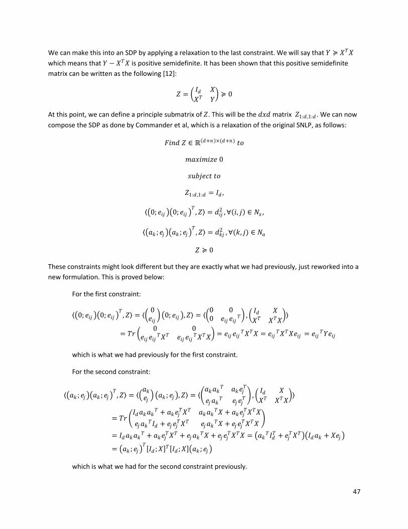
47

We can make this into an SDP by applying a relaxation to the last constraint. We will say that 𝑌 ≽ 𝑋𝑇𝑋

which means that 𝑌 − 𝑋𝑇𝑋 is positive semidefinite. It has been shown that this positive semidefinite

matrix can be written as the following [12]:

𝑍 = 𝐼𝑑 𝑋

𝑋𝑇 𝑌 ≽ 0

At this point, we can define a principle submatrix of 𝑍. This will be the 𝑑𝑥𝑑 matrix 𝑍1:𝑑 ,1:𝑑 . We can now

compose the SDP as done by Commander et al, which is a relaxation of the original SNLP, as follows:

𝐹𝑖𝑛𝑑 𝑍 ∈ ℝ 𝑑+𝑛 ×(𝑑+𝑛) 𝑡𝑜

𝑚𝑎𝑥𝑖𝑚𝑖𝑧𝑒 0

𝑠𝑢𝑏𝑗𝑒𝑐𝑡 𝑡𝑜

𝑍1:𝑑 ,1:𝑑 = 𝐼𝑑 ,

0; 𝑒𝑖𝑗 0; 𝑒𝑖𝑗 𝑇

, 𝑍 = 𝑑𝑖𝑗2 , ∀ 𝑖, 𝑗 ∈ 𝑁𝑥 ,

𝑎𝑘 ; 𝑒𝑗 𝑎𝑘 ; 𝑒𝑗 𝑇

, 𝑍 = 𝑑𝑘𝑗2 , ∀(𝑘, 𝑗) ∈ 𝑁𝑎

𝑍 ≽ 0

These constraints might look different but they are exactly what we had previously, just reworked into a

new formulation. This is proved below:

For the first constraint:

0; 𝑒𝑖𝑗 0; 𝑒𝑖𝑗 𝑇

, 𝑍 = 0𝑒𝑖𝑗

0; 𝑒𝑖𝑗 , 𝑍 = 0 00 𝑒𝑖𝑗 𝑒𝑖𝑗

𝑇 , 𝐼𝑑 𝑋

𝑋𝑇 𝑋𝑇𝑋

= 𝑇𝑟 0 0

𝑒𝑖𝑗 𝑒𝑖𝑗𝑇𝑋𝑇 𝑒𝑖𝑗 𝑒𝑖𝑗

𝑇𝑋𝑇𝑋 = 𝑒𝑖𝑗 𝑒𝑖𝑗𝑇𝑋𝑇𝑋 = 𝑒𝑖𝑗

𝑇𝑋𝑇𝑋𝑒𝑖𝑗 = 𝑒𝑖𝑗𝑇𝑌𝑒𝑖𝑗

which is what we had previously for the first constraint.

For the second constraint:

𝑎𝑘 ; 𝑒𝑗 𝑎𝑘 ; 𝑒𝑗 𝑇

, 𝑍 = 𝑎𝑘

𝑒𝑗 𝑎𝑘 ; 𝑒𝑗 , 𝑍 =

𝑎𝑘𝑎𝑘𝑇 𝑎𝑘𝑒𝑗

𝑇

𝑒𝑗𝑎𝑘𝑇 𝑒𝑗𝑒𝑗

𝑇 , 𝐼𝑑 𝑋

𝑋𝑇 𝑋𝑇𝑋

= 𝑇𝑟 𝐼𝑑𝑎𝑘𝑎𝑘

𝑇 + 𝑎𝑘𝑒𝑗𝑇𝑋𝑇 𝑎𝑘𝑎𝑘

𝑇𝑋 + 𝑎𝑘𝑒𝑗𝑇𝑋𝑇𝑋

𝑒𝑗𝑎𝑘𝑇𝐼𝑑 + 𝑒𝑗𝑒𝑗

𝑇𝑋𝑇 𝑒𝑗𝑎𝑘𝑇𝑋 + 𝑒𝑗𝑒𝑗

𝑇𝑋𝑇𝑋

= 𝐼𝑑𝑎𝑘𝑎𝑘𝑇 + 𝑎𝑘𝑒𝑗

𝑇𝑋𝑇 + 𝑒𝑗𝑎𝑘𝑇𝑋 + 𝑒𝑗𝑒𝑗

𝑇𝑋𝑇𝑋 = 𝑎𝑘𝑇𝐼𝑑

𝑇 + 𝑒𝑗𝑇𝑋𝑇 𝐼𝑑𝑎𝑘 + 𝑋𝑒𝑗

= 𝑎𝑘 ; 𝑒𝑗 𝑇 𝐼𝑑 ; 𝑋 𝑇 𝐼𝑑 ; 𝑋 𝑎𝑘 ; 𝑒𝑗

which is what we had for the second constraint previously.

48

The dual of this SDP is:

𝑚𝑖𝑛𝑖𝑚𝑖𝑧𝑒 𝐼𝑑 , 𝑉 + 𝑦𝑖𝑗 𝑑𝑖𝑗2

𝑖 ,𝑗 ∈𝑁𝑥

+ 𝑤𝑘𝑗 𝑑𝑘𝑗2

𝑘,𝑗 ∈𝑁𝑎

𝑠𝑢𝑏𝑗𝑒𝑐𝑡 𝑡𝑜

𝑉 00 0

+ 𝑦𝑖𝑗 0; 𝑒𝑖𝑗 0; 𝑒𝑖𝑗 𝑇

(𝑖,𝑗 )∈𝑁𝑥

+ 𝑤𝑘𝑗 𝑎𝑘 ; 𝑒𝑗 𝑎𝑘 ; 𝑒𝑗 𝑇

(𝑘 ,𝑗 )∈𝑁𝑎

≽ 0

So and Ye, in their paper Theory of Semidefinite Programming for Sensor Network Localization [13],

provide many results of this representation of the SNLP. One important result, describes a set of

instances where this SDP relaxation is exact. This occurs when the feasible solution, 𝑍, has rank 𝑑. The

theorem is stated below:

Theorem: Let Z be a feasible solution for SDP and U be an optimal slack matrix of SDP-D. Then, by the

duality theorem for semidefinite programming, it follows that:

1. 𝑍 , 𝑈 = 0

2. 𝑟𝑎𝑛𝑘 𝑍 + 𝑟𝑎𝑛𝑘 𝑈 ≤ 𝑑 + 𝑛

3. 𝑟𝑎𝑛𝑘 𝑍 ≥ 𝑑 𝑎𝑛𝑑 𝑟𝑎𝑛𝑘 𝑈 ≤ 𝑛

This means, if you have an optimal slack matrix for the dual with rank 𝑛, then the rank of 𝑍 will be 𝑑

[12]. This is because of the above inequalities. If 𝑟𝑎𝑛𝑘 U = 𝑛 then you have 𝑟𝑎𝑛𝑘 Z + 𝑛 ≤ 𝑑 + 𝑛.

This can be simplified to 𝑟𝑎𝑛𝑘 Z ≤ 𝑑. But by the 3rd condition, we also have that 𝑟𝑎𝑛𝑘 Z ≥ 𝑑. So

𝑟𝑎𝑛𝑘 Z must equal 𝑑. The main result from this is that we can say the original SNLP is equal to the SDP

relaxation meaning the SNLP can be solved in polynomial time.

So and Ye have another important conclusion that states there exists a big group of localizable graphs

that can be solved efficiently [13]. This theorem is stated below:

Theorem: Suppose that the network in question is connected. Then the following are equivalent:

1. Problem SNLP is uniquely localizable

2. The max-rank solution matrix of SDP has rand d

3. The solution matrix, Z, of SDP satisfies 𝑌 = 𝑋𝑇𝑋

This result further emphasizes that the SNLP can be solved in polynomial time by using the SDP

relaxation we derived above. This is as long as the SNLP is uniquely localizable. This holds for the reverse

too. This theorem also introduces the fact that there is a group of graphs for which was can figure out

the localization even though the general SNLP is NP-Complete [12].

Knowing that the solution to the SDP will provide the optimal solution for the SNLP, we can utitlize the

interior point method of Helmberg et al. to solve.

49

4 NEOS Guide

For this project, the SNLPs were solved using the interior point method described earlier. This was done

using computer software because, while we have the algorithm for solving the SNLP, it is not very easy

to do by hand. Like many optimization problems, we need the use of computers to arrive at our

solution. The NEOS Solver is optimization software that can solve most any type of optimization

problem. It has applications in semidefinite programming which we can utilize to solve our SNLP. We

can obtain the NEOS Solver online where it functions as a type of cloud computing. This means that

when we enter the data for our problem, it gets sent off to a university or company that owns the

software. There the problem is solved, the solution is sent back to NEOS and NEOS provides it to us.

This is usually done through email, however if the problem does not take long to solve, it will show the

answer in the browser window. In an effort to utilize the NEOS software and analyze our solution, I

studied the NEOS program to understand the formats and the ideas behind it. I also created MAPLE

codes to aid us in our use of NEOS.

I will use a simple example in an effort to explain these programs and the process to follow to solve an

SNLP. Our SNLP example consists of 5 anchors and 4 nodes. The positions of the anchors are

0,0 , 4, 0 , 3, 6 , 0, 3 and (6, 3). We have 8 anchor-node measurements and 4 node-node

measurements. We are trying to obtain the positions of the 4 nodes given the anchor positions and the

measurements. We will continue to refer to this example to help illustrate the descriptions that follow.

4.1 NEOS Input and Output

While NEOS Solvers can make our work very easy, it requires specific input and provides solutions in a

similarly specific output. The format of the input and output is dependent on the type of solver we are

choosing to use. In our situation, with the SNLP, we employed the semidefinite programming solver for

CSDP.

4.1.1 Input

I first looked at the NEOS input. The input is very specific and we can only formulate it once we have all

the needed information. This means we must first understand what information we need and how to

obtain it.

The input consists of six sections defined as follows [14]:

1. Comments: there can be as many lines of comments as the user wants however each line must

begin with ‘”’ or ‘*’. While comments can be used, it is often advised not to in order to avoid any

confusion with the solver.

2. The number of constraint matrices

3. The number of blocks in the block diagonal matrices

4. List of numbers that give the size of the individual blocks. Note: Negative numbers are allowed

and should be used for a block where the diagonals are the only nonzero entries.

5. The objective function vector

50

6. Entries of the constraint matrices with one entry on each line. Each line will have the format:

matrix, block, row, column, value. Since all the matrices are assumed to be symmetric, only the

upper triangle entries of the matrix are needed.

Now that we know what information is needed, we must understand how to obtain it. Let us first

remember our SNLP problem. It is stated as an SDP in the following form:

𝑚𝑎𝑥𝑖𝑚𝑖𝑧𝑒 0

𝑠𝑢𝑏𝑗𝑒𝑐𝑡 𝑡𝑜

𝑍1:𝑑 ,1:𝑑 = 𝐼𝑑 ,

0; 𝑒𝑖𝑗 0; 𝑒𝑖𝑗 𝑇

, 𝑍 = 𝑑𝑖𝑗2 , ∀ 𝑖, 𝑗 ∈ 𝑁𝑥 ,

𝑎𝑘 ; 𝑒𝑗 𝑎𝑘 ; 𝑒𝑗 𝑇

, 𝑍 = 𝑑𝑘𝑗2 , ∀(𝑘, 𝑗) ∈ 𝑁𝑎

𝑍 ≽ 0

We can rewrite the second and third constraints as:

𝑒𝑖𝑗𝑇𝑌𝑒𝑖𝑗 = 𝑑𝑖𝑗

2 , ∀ 𝑖, 𝑗 ∈ 𝑁𝑥 ,

𝑎𝑘 ; 𝑒𝑗 𝑇 𝐼𝑑 𝑋

𝑋𝑇 𝑌 𝑎𝑘 ; 𝑒𝑗 = 𝑑𝑘𝑗

2 , ∀(𝑘, 𝑗) ∈ 𝑁𝑎

by applying the definition of 𝑍 which is, 𝑍 = 𝐼𝑑 𝑋

𝑋𝑇 𝑌 . Remember that 𝑎𝑘 is the position vector of the

anchor 𝑘, 𝑒𝑗 is the vector of length n of all zeros except at −1 in the jth position, and 𝑒𝑖𝑗 is the vector of

length 𝑛 of all zeros except 1 at the ith position and −1 at the jth position.

To begin we want to find the constraint matrices which are needed to provide information for the NEOS

input lines 2, 3, 4, and 6. The way to formulate these matrices is fairly simple but tedious. For the

anchor-node constraints we must compute 𝑎𝑘 ; 𝑒𝑗 𝑇 𝑎𝑘 ; 𝑒𝑗 for each distance known. For the node-

node constraints we must compute 𝑒𝑖𝑗𝑇𝑒𝑖𝑗 for each distance known. Utilizing the defined example above,

we will demonstrate this process.

For the anchor-node constraint we will use the measurement of anchor 2 to node 4. This distance is 2.

The constraint matrix will be:

40⋯000

−1

4 0 ⋮ 0 0 0 −1 =

16 0 0 0 0 −40 0 0 0 0 0000

−4

0000

0000

0000

0000

0001

51

We will do similarly for the node-node constraints. We will use the node-node measurement of node 1

and node 2. The distance is 2. The constraint matrix will be:

1−100

1 −1 0 0 =

1 −1 0 0−100

100

000

000

These matrices will be the majority of our constraint matrices. The last three matrices will be used to

force 𝑍1:𝑑 ,1:𝑑 = 𝐼𝑑 . The first of these will be a matrix of all zeros except for a 1 in the 1, 1 spot. The

second will be all zeros except for a 1 in the 2, 2 spot. Finally, the third will also be all zeros except for a

1 in the 2, 1 spot. This is how we will construct all of our constraint matrices.

We now have almost all of the information we need to create the NEOS output. The last piece is the

objective function vector needed in line 5. This will be made up of the known distances 𝑑𝑖𝑗2 and 𝑑𝑘𝑗

2 .

They will be presented in the same order of the corresponding constraint matrices. So if we decide that

our anchor-node example above is the first constraint matrix, then out first distance in the objective

function vector will be 2, the corresponding distance. For the last three matrices, we will have 1, 1, 0

corresponding to the first, second, and third matrix. This will force the values in the matrices to the

identity matrix values.

We now should be able to understand how to obtain the necessary information for the NEOS input.

Here is part of the NEOS input for our simple example.

Size of blocks

Entries of constraint matrices with format:

Matrix, Block, Row, Column, Value

Objective function vector

Number of blocks Number of constraint matrices

52

4.1.2 Output

Once we have the data in this format and we submit it to NEOS, we will obtain the solution back in the

specific output format. The NEOS output will be in a similar format as the input however it just presents

matrix values. These matrix values are of our solution matrix 𝑍. Below is the output for our example.

Now that we understand the NEOS formats, we can utilize the software to solve our SNLPs.

4.2 MAPLE CODES

Even though it might be enough to understand the input and output files, converting our SNLP into this

format and deciphering the output might be very tedious by hand, especially with many nodes and

anchors. For this reason, I have developed MAPLE codes to perform this work. The first code takes all

Entries of our solution matrices with format:

Matrix, Block, Row, Column, Value

53

the sensor network data, provided in a very easy to use format, and converts it into the proper NEOS

format. Once the solution is provided by NEOS, the second code takes the output, converts it into matrix

form, and then plots the anchors and nodes onto a coordinate graph. We will continue to use our simple

example to help explain the codes and the process for their use.

4.2.1 Data File

To begin, we receive, or compile ourselves, the data describing the SNLP in a very simple format. We

write up the information into a text document called “data.” The format of this file is as follows:

1. Number of anchors

2. Anchor positions with one position for each line in the format: node, x-coord., y-coord.

3. Number of anchor-node measurements

4. Anchor-node measurements in format: anchor, node, measurement

5. Number of node-node measurements

6. Node-node measurements in format: node, node, measurement

Here is the data file for our given example:

5

1 0 0

2 4 0

3 3 6

4 0 3

5 6 3

8

1 1 2.8284

2 4 2.0

3 2 2.2361

3 3 2.2361

4 1 2.2361

4 2 2.2361

5 4 2.2361

5 3 2.2361

4

1 2 2.0

54

2 3 2.0

3 4 2.0

4 1 2.0

4.2.2 MAPLE Code 1: Data to NEOS Input

Once we have our data file, we then open our first MAPLE code. This code takes our data file and converts it into the NEOS input format explained above. The MAPLE code is displayed below. A key thing to note is that prior executing the code, we must change the current directory in this code to the directory that our data file is stored in.

> # Input data for sensor network SDP and print csdp format as output.

d:=2: # Assume 2-dimensional for now

# Open file "data" for reading. Contents are assumed to be in TEXT format.

# File pointer for this file is fp.

currentdir("C:/Users/bhegarty/Desktop");

fp := fopen(data,READ,TEXT);

# Get number of anchors.

inlist := fscanf(fp,"%d");

k := inlist[1];

# Initialize all anchors to (0,0).

Anchors := matrix(k,d,0):

# For each anchor, read its label and (x,y)-coords.

for i to k

do

inlist := fscanf(fp,"%d %f %f");

if nops( inlist ) < 3 then print(`ERROR: Ran out of data while reading anchors`);

i := k;

else j := inlist[1]; Anchors[j,1] := inlist[2]; Anchors[j,2] := inlist[3];

fi

od;

# Get number of anchor-node measurements.

inlist := fscanf(fp,"%d");

if nops( inlist ) < 1 then

print(`ERROR: Ran out of data while reading number of anchor-node measurements.`);

else

55

AN := inlist[1];

# Initialize all entries to zero.

ANlist := matrix(AN,3,0):

# For each measurement, store: anchor label, sensor label, distance.

for i to AN

do

inlist := fscanf(fp,"%d %d %f");

if nops( inlist ) < 3 then print(`ERROR: Ran out of data while reading AN measurements`);

i := AN;

else if inlist[1] > k then printf(`ERROR: in anchor-node pair %d, node index %d out of

range.\n`,

i, inlist[1]);

else ANlist[i,1] := inlist[1]; ANlist[i,2] := inlist[2]; ANlist[i,3] := inlist[3];

fi fi

od;

fi;

# Get number of node-node measurements.

inlist := fscanf(fp,"%d");

if nops( inlist ) < 1 then

print(`ERROR: Ran out of data while reading number of node-node measurements.`);

else

NN := inlist[1];

# Initialize all entries to zero.

NNlist := matrix(NN,3,0):

# For each measurement, store: sensor label, sensor label, distance.

for i to NN

do

inlist := fscanf(fp,"%d %d %f");

if nops( inlist ) < 3 then print(`ERROR: Ran out of data while reading NN measurements`);

i := NN;

else NNlist[i,1] := inlist[1]; NNlist[i,2] := inlist[2]; NNlist[i,3] := inlist[3];

# Keep convention that smaller node is first.

if NNlist[i,1] > NNlist[i,2] then # swap

tempval := NNlist[i,1]; NNlist[i,1] := NNlist[i,2]; NNlist[i,2] := tempval;

fi

56

fi

od;

fi;

# Now figure out the number of sensors (= biggest label that appeared).

n := max( seq( ANlist[h,2],h=1..AN), seq( NNlist[h,2],h=1..NN) );

# For debugging purposes, now report all data collected

print(`k=`,k,`n=`,n,`AN=`,AN,`NN=`,NN);

op(Anchors), op(ANlist), op(NNlist);

# Now we can give the neos input. Start with an easy-to-locate line.

print(`Now we give the input file for the csdp neos solver.`);

printf(`neosneosneosneosneosneosneosneosneosneosneosneosneosneosneosneosneosneos\n`);

printf(`%d\n1\n%d\n`,AN+NN+3,n+2): # num. constraints, num. blocks, block size

# Now print objective coefficients

printf(`%2.1f `,ANlist[1,3]^2*1.0):

for i from 2 to AN do printf(`%5.1f `,ANlist[i,3]^2*1.0); od:

printf(` `):

for i to NN do printf(`%5.1f `,NNlist[i,3]^2*1.0); od:

printf(` 1.0 1.0 0.0\n`):

for i to AN # Build all constraints for anchor-node measurements

do

anc := ANlist[i,1]: nod := ANlist[i,2]:

printf(`%2d 1 1 1 %5.1f\n`,i,Anchors[anc,1]^2*1.0);

printf(`%2d 1 1 2 %5.1f\n`,i,Anchors[anc,1]*Anchors[anc,2]*1.0);

printf(`%2d 1 2 2 %5.1f\n`,i,Anchors[anc,2]^2*1.0);

printf(`%2d 1 1 %2d %5.1f\n`,i,2+nod,Anchors[anc,1]*1.0);

printf(`%2d 1 2 %2d %5.1f\n`,i,2+nod,Anchors[anc,2]*1.0);

printf(`%2d 1 %2d %2d %5.1f\n`,i,2+nod,2+nod,1.0);

od:

for i to NN # Build all constraints for node-node measurements

do

n1 := NNlist[i,1]: n2 := NNlist[i,2]:

printf(`%2d 1 %2d %2d 1.0\n`,AN+i,2+n1,2+n1);

printf(`%2d 1 %2d %2d -1.0\n`,AN+i,2+n1,2+n2);

printf(`%2d 1 %2d %2d 1.0\n`,AN+i,2+n2,2+n2);

57

od:

# Finally, force 2x2 identity matrix in upper-left

# corner of psd variable Z

printf(`%2d 1 1 1 1.0\n`,AN+NN+1);

printf(`%2d 1 2 2 1.0\n`,AN+NN+2);

printf(`%2d 1 1 2 1.0\n`,AN+NN+3);

quit

This program will then provide us with our NEOS input. For our example, this input is:

15

1

6

8.0 4.0 5.0 5.0 5.0 5.0 5.0 5.0 4.0 4.0 4.0 4.0 1.0 1.0 0.0

1 1 1 1 0.0

1 1 1 2 0.0

1 1 2 2 0.0

1 1 1 3 0.0

1 1 2 3 0.0

1 1 3 3 1.0

2 1 1 1 16.0

2 1 1 2 0.0

2 1 2 2 0.0

2 1 1 6 4.0

2 1 2 6 0.0

2 1 6 6 1.0

3 1 1 1 9.0

3 1 1 2 18.0

3 1 2 2 36.0

3 1 1 4 3.0

3 1 2 4 6.0

3 1 4 4 1.0

4 1 1 1 9.0

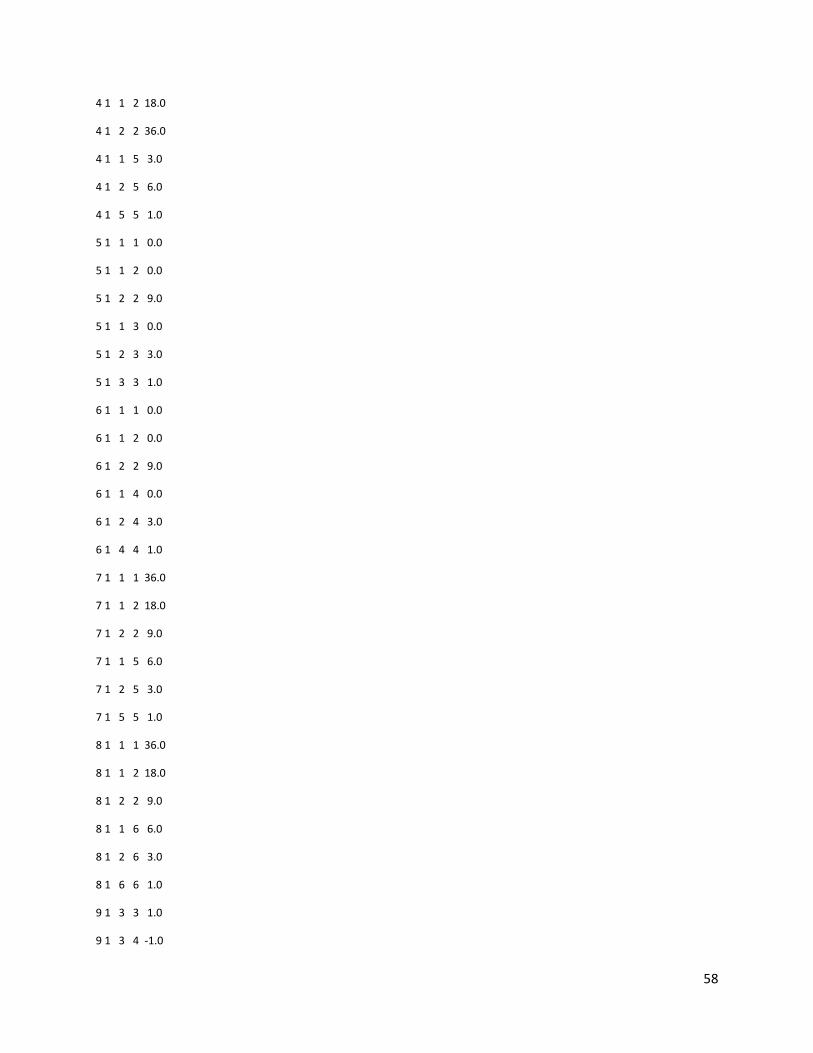
58

4 1 1 2 18.0

4 1 2 2 36.0

4 1 1 5 3.0

4 1 2 5 6.0

4 1 5 5 1.0

5 1 1 1 0.0

5 1 1 2 0.0

5 1 2 2 9.0

5 1 1 3 0.0

5 1 2 3 3.0

5 1 3 3 1.0

6 1 1 1 0.0

6 1 1 2 0.0

6 1 2 2 9.0

6 1 1 4 0.0

6 1 2 4 3.0

6 1 4 4 1.0

7 1 1 1 36.0

7 1 1 2 18.0

7 1 2 2 9.0

7 1 1 5 6.0

7 1 2 5 3.0

7 1 5 5 1.0

8 1 1 1 36.0

8 1 1 2 18.0

8 1 2 2 9.0

8 1 1 6 6.0

8 1 2 6 3.0

8 1 6 6 1.0

9 1 3 3 1.0

9 1 3 4 -1.0

59

9 1 4 4 1.0

10 1 4 4 1.0

10 1 4 5 -1.0

10 1 5 5 1.0

11 1 5 5 1.0

11 1 5 6 -1.0

11 1 6 6 1.0

12 1 3 3 1.0

12 1 3 6 -1.0

12 1 6 6 1.0

13 1 1 1 1.0

14 1 2 2 1.0

15 1 1 2 1.0

4.2.3 MAPLE Code 2: NEOS Output to Matrix and Graph

After submitting this to NEOS, we will receive the NEOS solution. It will be in the format explained

above. For our example, we receive this output (as previously shown):

1 1 1 1 1.000000000496007042e-50

1 1 1 2 8.717591509285441338e-62

1 1 1 3 -1.999999999670224407e-50

1 1 1 4 -2.000000001814057016e-50

1 1 1 5 -3.999999999101171427e-50

1 1 1 6 -3.999999998755753059e-50

1 1 2 2 1.000000000474183616e-50

1 1 2 3 -2.000000000119852597e-50

1 1 2 4 -3.999999998731452951e-50

1 1 2 5 -3.999999999021356433e-50

1 1 2 6 -2.000000001296558545e-50

1 1 3 3 8.000000000416214534e-50

1 1 3 4 1.199999999594339242e-49

1 1 3 5 1.599999998798805185e-49

60

1 1 3 6 1.199999999416303804e-49

1 1 4 4 1.999999999222064470e-49

1 1 4 5 2.399999998522994746e-49

1 1 4 6 1.599999999912987757e-49

1 1 5 5 3.199999997911535359e-49

1 1 5 6 2.399999998371298494e-49

1 1 6 6 1.999999998877663647e-49

2 1 1 1 1.000000000496007013e+00

2 1 1 2 8.717591509285440713e-12

2 1 1 3 -1.999999999670224460e+00

2 1 1 4 -2.000000001814056905e+00

2 1 1 5 -3.999999999101171433e+00

2 1 1 6 -3.999999998755753072e+00

2 1 2 2 1.000000000474183581e+00

2 1 2 3 -2.000000000119852572e+00

2 1 2 4 -3.999999998731452955e+00

2 1 2 5 -3.999999999021356611e+00

2 1 2 6 -2.000000001296558416e+00

2 1 3 3 8.000000000416214618e+00

2 1 3 4 1.199999999594339251e+01

2 1 3 5 1.599999998798805123e+01

2 1 3 6 1.199999999416303709e+01

2 1 4 4 1.999999999222064417e+01

2 1 4 5 2.399999998522994815e+01

2 1 4 6 1.599999999912987825e+01

2 1 5 5 3.199999997911535488e+01

2 1 5 6 2.399999998371298560e+01

2 1 6 6 1.999999998877663643e+01

61

We then take this output, copy it, and paste it into a text file called “fromneos.” After creating this file,

we open MAPLE again and use our next code which will take the NEOS output and display it in matrix

and graphical form. This code is shown below:

(Note again that the directory must be correct for the code to work.)

> currentdir("C:/Users/bhegarty/Desktop");

> # File pointer for this file is neosfp.

neosfp := fopen(fromneos,READ,TEXT);

# File pointer for data file is dfp.

dfp := fopen(data,READ,TEXT);

L := [];

# For each line, store it as a 5-tuple in L

ans := fscanf(neosfp,"%d %d %d %d");

while nops( ans ) > 0

do

xx := fscanf(neosfp,"%g");

L := [ op(L), [ op(ans), op(xx) ] ];

ans := fscanf(neosfp,"%d %d %d %d");

od:

fclose(neosfp);

> # Now get original data to find anchors and graph:

# Get number of anchors.

inlist := fscanf(dfp,"%d");

k := inlist[1];

# Initialize list of anchors to empty

anchors := [];

# For each anchor, store (x,y)-coords.

for i to k

do

inlist := fscanf(dfp,"%d %f %f");

if nops( inlist ) < 3 then print(`ERROR: Ran out of data while reading anchors`);

i := k;

else anchors:= [op(anchors), [inlist[2], inlist[3]]];

fi

od;

62

> # Get number of anchor-node measurements.

inlist := fscanf(dfp,"%d");

if nops( inlist ) < 1 then

print(`ERROR: Ran out of data while reading number of anchor-node measurements.`);

else

AN := inlist[1];

# Initialize list of anchor node edges to empty

aedges:=[];

andist:=[];

# For each measurement, store: anchor label, sensor label, distance.

for i to AN

do

inlist := fscanf(dfp,"%d %d %f");

if nops( inlist ) < 3 then print(`ERROR: Ran out of data while reading AN measurements`);

i := AN;

else if inlist[1] > k then printf(`ERROR: in anchor-node pair %d, node index %d out of

range.\n`, i, inlist[1]);

else aedges:=[op(aedges), [inlist[1], inlist[2]]]; andist:= [op(andist), inlist[3]];

fi fi

od;

fi;

> aedges, andist, indist, AN;

> # Get number of node-node measurements.

inlist := fscanf(dfp,"%d");

if nops( inlist ) < 1 then

print(`ERROR: Ran out of data while reading number of node-node measurements.`);

else

NN := inlist[1];

> # Initialize list of node node edges to empty

xedges:=[]; nndist:=[]; # For each measurement, store: sensor label, sensor label, #

#distance.

for i to NN

do

inlist := fscanf(dfp,"%d %d %f");

if nops( inlist ) < 3 then print(`ERROR: Ran out of data while reading NN measurements`);

63

i := NN;

else xedges:=[op(xedges),[inlist[1], inlist[2]]]; nndist:=[op(nndist), inlist[3]];

# Keep convention that smaller node is first.

####(Don't think this works because inlist[1] is more of a command, not a value

#### Does it matter that to have it in numerical order?)

if inlist[1] > inlist[2] then #swap

tempval:= inlist[1]; inlist[1]:= inlist[2]; inlist[1]:=tempval;

fi

fi

od;

fi;

> # now get actual matrix from neos output

numdigs := 3;

numvals := nops(L); # How many entries in the list?

size := max( seq( L[i][4], i=1..numvals) ); # find size of matrix

B := matrix(size,size, 0.):

for i to numvals

do

row := L[i][3]; col := L[i][4];

B[ row, col] := round( 10^numdigs * L[i][5])/(10.^numdigs) ;

B[ col, row] := round( 10^numdigs * L[i][5])/(10.^numdigs) ;

od:

op(B);

getX := proc(B) # Given matrix B, pull off coords of all points x_i

local Pts, h, size;

size := linalg[coldim](B);

Pts := [ seq( [B[1,h],B[2,h] ], h=3..size) ];

RETURN( Pts );

end;

#get nodes from matrix

Points:= -getX(B);

> numanchors := nops( anchors );

numPoints := nops( Points );

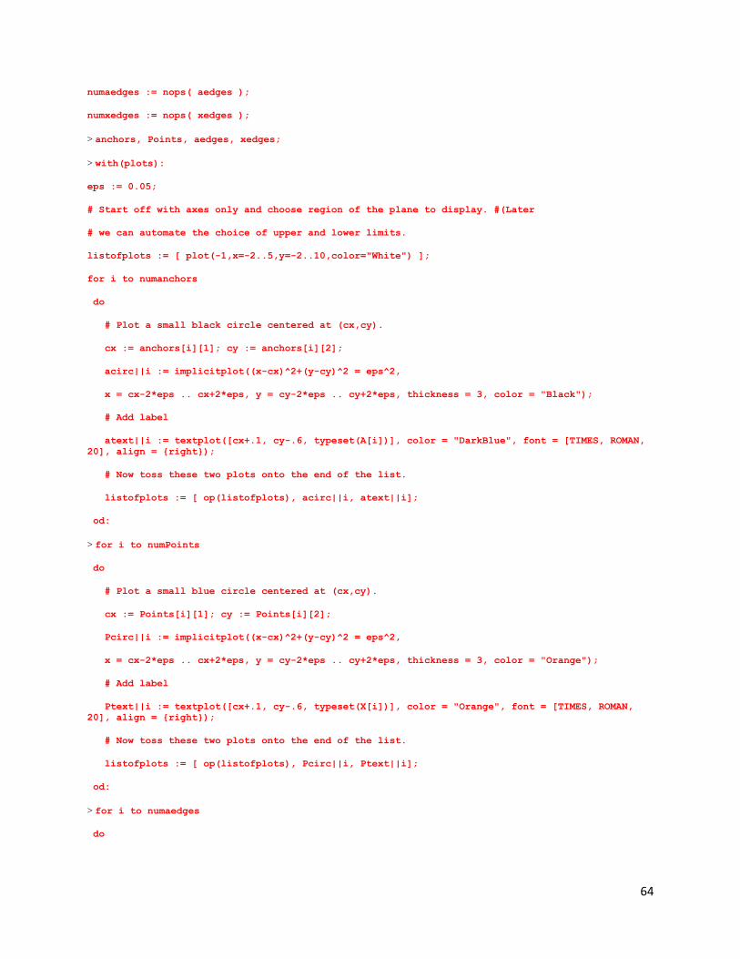
64

numaedges := nops( aedges );

numxedges := nops( xedges );

> anchors, Points, aedges, xedges;

> with(plots):

eps := 0.05;

# Start off with axes only and choose region of the plane to display. #(Later

# we can automate the choice of upper and lower limits.

listofplots := [ plot(-1,x=-2..5,y=-2..10,color="White") ];

for i to numanchors

do

# Plot a small black circle centered at (cx,cy).

cx := anchors[i][1]; cy := anchors[i][2];

acirc||i := implicitplot((x-cx)^2+(y-cy)^2 = eps^2,

x = cx-2*eps .. cx+2*eps, y = cy-2*eps .. cy+2*eps, thickness = 3, color = "Black");

# Add label

atext||i := textplot([cx+.1, cy-.6, typeset(A[i])], color = "DarkBlue", font = [TIMES, ROMAN,

20], align = {right});

# Now toss these two plots onto the end of the list.

listofplots := [ op(listofplots), acirc||i, atext||i];

od:

> for i to numPoints

do

# Plot a small blue circle centered at (cx,cy).

cx := Points[i][1]; cy := Points[i][2];

Pcirc||i := implicitplot((x-cx)^2+(y-cy)^2 = eps^2,

x = cx-2*eps .. cx+2*eps, y = cy-2*eps .. cy+2*eps, thickness = 3, color = "Orange");

# Add label

Ptext||i := textplot([cx+.1, cy-.6, typeset(X[i])], color = "Orange", font = [TIMES, ROMAN,

20], align = {right});

# Now toss these two plots onto the end of the list.

listofplots := [ op(listofplots), Pcirc||i, Ptext||i];

od:

> for i to numaedges

do

65

listofplots := [ op(listofplots) , plot( [ anchors[aedges[i][1]], Points[aedges[i][2]]

],color="Green") ];

od:

> for i to numxedges

do

listofplots := [ op(listofplots) , plot( [ Points[xedges[i][1]], Points[xedges[i][2]]

],color="Blue",thickness=2) ];

od:

display( listofplots);

Using this code for our example, we will receive the following representations of the solution:

Matrix:

Graph:

66

5 Conclusion and Further Work

Vast benefits of semidefinite programming have already been noted by many experts, and I believe

more are to be discovered in the future. This project focused on the understanding of this new and

exciting topic in mathematics and how it can be applied to the real world. It began by giving an

introduction into the basic theory behind semidefinite programming. It then discussed a method for SDP

solution: the interior point method. Next, it surveyed a variety of applications, elaborating on that of

the sensor networks. Lastly, it presented computer based tools that can be used to solve given SNLPs.

While this project covered the theory of semidefinite programming, its methods for its solution, and its

application to sensor networks, more work can be done. I believe the next step is to investigate the

SNLP with noisy data, referring to the utilization of measurements which are not exact. Also, the

development of a user friendly and interactive graph, which displays the solution to the sensor network

being studied, would be very advantageous to those not as familiar with these topics of advanced

mathematics.

67

6 References

[1] C. Helmberg, F. Rendl, R. Vanderbei, and H. Wolkowicz, An Interior-Point Method for Semidefinite

Programming, SIAM J. Optim., 6 (1996), pp.342-361.

[2] R. Vanderbei. Linear Programming: Foundations and Extensions. Springer, New York, (2008), pp.287-

318.

[3] J. B. Lasserre, Why the Logarithmic Barrier Function in Convex and Linear Programming, Operations

Research Letters, 27 (2000), pp.149-152.

[4] “Line Search Methods.” Wolfram Mathematica: Documentation Center, Wolfram Research Inc,

(2010).

http://reference.wolfram.com/mathematica/tutorial/UnconstrainedOptimizationLineSearchMethods.ht

ml.

[5] M. Goemans and D. Williamson, Improved Approximation Algorithms for Maximum Cut and

Satisfiability Problems Using Semidefinite Programming, JACM, 42 (1995), pp. 1115-1145.

[6] J. Wheeler, An Investigation of the MaxCut Problem, Internal Report, University of Iowa, 2004.

[7] A. Kojevnikov and A. S. Kulikov, New Approach to Proving Upper Bounds for MAX-2-SAT, SODA

(2006), pp. 11-17.

[8] Professor W. J. Martin, 2009-2010, Personal communication through weekly meetings.

[9] A. Schrijver, New Code Upper Bounds from the Terwilliger Agebra, IEEE Transactions on Information

Theory 51 (2005) pp. 2859-2866.

[10] A.S. Lewis, The Mathematics of Eigenvalue Optimization, Mathematical Programming, 97 (2003),

pp. 155-176.

[11] I. Popescu and D. Bertsimas, Moment Problems via Semidefinite Programming: Applications in

Probability and Finance, Working Paper, MIT, Cambridge, MA (2000).

[12] C. Commander, M. Ragle and Y. Ye, Semidefinite Programming and the Sensor Network Localization

Problem, SNLP, Encyclopedia of Optimization, 2007.

[13] A. So and Y. Ye, Theory of Semidefinite Programming for Sensor Networks Localization,

Mathematical Programming, 2006.

[14] NEOS: Server for Optimization,

http://neos.mcs.anl.gov/neos/solvers/sdp:csdp/MATLAB_BINARY.html.