DEPARTMENT OF MATHEMATICS

ST.THOMAS’ COLLEGE

Thrissur 680001, Thrissur District, Kerala state

TEL-0487 2420435, FAX-0487 2421510 Email-stcthrissur@gmail.com

CERTIFICATE

Certified that this project report titled “NUMERICAL METHODS OF SOLVING

PARTIAL DIFFERENTIAL EQUATIONS’’ submitted by LINTU RAJ Reg No.

THAMMMS011, to the university of Calicut, in partial fulfillment of the requirement

for the Degree of Master of Science in Mathematics, is a bonafide work undertaken

by her under our supervision during the year 2013-2014.

PROJECT SUPERVISOR HEAD OF DEPARTMENT

Prof. SABU A.S Dr .P.L Antony

Assistant Professor Associate Professor

THRISSUR

DECLARATION

I LINTU RAJ,Re.No-THAMMMS011, do here by declare that the project

entitled “NUMERICAL METHODS FOR SOLVING PARTIAL DIFFERENTIAL

EQUATIONS’’ to the Department of Mathematics, St. Thomas’ College Thrissur, is

an original dissertation done by me under the supervision of Prof. SABU A.S.

Assistant Professor of Mathematics Department of St.Thomas’ College, Thrissur.

THRISSUR LINTU RAJ

Reg No: THAMMMS011

ACKNOWLEDGEMENT

This is project which is prepared in the light of my interest in Partial

differential equations concentrating on the topic entitled “ NUMERICAL

METHODS FOR SOLVING PARTIAL DIFFERENTIAL EQUATIONS .’’ Firstly

I thank GOD almighty for the holy support given to me throughout the work of

the project . It is my proud privilege to express my sincere gratitude and deep

indebtedness to the people who helped me to complete the project work successfully

I am deeply grateful to our principal Dr. JENSON P. O for providing all the

facility to do this project.

I am indebted to Dr. P. L ANTONY(Head of the Department of mathematics

St.Thomas’ College, Thrissur ),for encouragement in carrying out this project and

also for the facilities provided to us.

I would like to express our sincere gratitude to Mr. SABU A.S. (Assistant

Professor, Department of Mathematics) for his valuable advices and whole hearted

cooperation in the fulfillment of my project.I express my sincere thanks gratitude to

all faculty of the Department and to librarians of our college who helped me

referring the related books. And of course, I thank all my classmates and my family

for their sincere co-operation.

LINTU RAJ

CONTENT

CHAPTER 1 ……………………………………………………. 1

INTRODUCTION

CHAPTER 2 …………………………………………. ……….. 2

PRELIMINARIES

CHAPTER 3 …………………………………………………..... 9

NUMERICAL METHODS FOR SOLVING

PARTIAL DIFFERENTIAL EQUATIONS

CHAPTER 4 …………………………………………………… 31

APPLICATIONS

BIBLIOGRAPHY……………………………………………. …..35

CHAPTER 1

INTRODUCTION

Partial differential equation arise in the study of many branches of

applied mathematics , for example fluid dynamics , heat transfer, boundary layer

flow, elasticity, quantum mechanics and electromagnetic theory. Only a few of these

equations can be solved by analytical method which are also complicated requiring

use of advanced mathematical techniques. In most of these cases it is easier to

develop approximate solutions by numerical methods . Of all the numerical methods

available for the solutions of partial equations, the method of finite difference is

most commonly used. In this method, the derivative appearing in the equations

and the boundary conditions are replaced by their finite difference approximations.

Then the given equations is changed to a system of linear equations which are

solved by iterative procedure. This process is slow but procedure good result in

many boundary value problem.

An added advantage of this method is that the

computation can be carried by electronic computers . To accelerate the solution

sometimes the method of relaxation proves quite effective. The another methods for

the numerical solutions of partial differential equations are finite element method,

finite volume method, spectral method, mesh free method, domain decomposition

method, multi grid method, methods of lines, etc.

[1]

CHAPTER 2

PRELIMINARIES

PARTIAL DIFFERENTIAL EQUATIONS

By a partial differential equations (P.D.E) we mean an equation of the form

f( x,y,t,……..,Ѳx,Ѳy……,Ѳxy,…..)=0 involving two or more independent variables

x,y,t,… etc one independent variable Ѳ(x,y,t,…) € Cn

in some domain D and its

partial derivatives Ѳx, Ѳy,….. , Ѳxx , Ѳyy , Ѳxy, …. Where Cn denote a set of

functions possessing continuous partial derivatives of order n. A partial differential

equation is thus a reletion between the dependent variable Ѳ and some of partial

derivatives at every point (x,y,t,…..) in D . A partial differential equation is an

equation that involves an unknowen function (the dependent variable) and some of

its partial derivatives with respect to two or more independent variable . An nth

order equation has the heighest order derivative of order n.

Second Order Partial Differential Equations

A partial differential equation is said to be second order semi linear partial

differential equation if it can be put in the form

R(x,y) Uxx+ S(x,y) UXY+ T(x,y) UYY+ g(x,y,U,Ux,Uy) = 0

Where , R2+S

2+T

2 ≠0 and R ,S and T are continuous .

[2]

Classical Equations of Mathematical Physics

1. Laplace equation (The potential equation)

2 =0

In cartesian coordinates , the vector operator Laplace del is defined as

= ex x

+ ey

y

+ ez

z

2 is refered as the Laplacian operator and given by

2

= . = 2

2

x

+

2

2

y

+

2

2

z

Thus Laplace equation in cartesian co-ordinates is

2

2

x

+

2

2

y

+

2

2

z

= 0

Laplace equation arises in incompressible fluid flow , gravitational

potential problems , electrostatics , magnetostics , study state heat conduction with

no source and torsion of bars in elasticity. Function which satisfies Laplace

equation are referred to as harmonic functions.

2. Poisson’s Equation

Ф2

+ g = 0

This equation arises in study state heat conduction with distributed sources

( = temperature) and tostion of bar in elasticity (in which case (x,y) is

the stress functions ).

[3]

3. Wave Equation

2 = 1/C

2

In this equations , dots denotes time derivatives ,

= 2

2

t

And C is the speed propagation.

4. Helmhotlz Equations ( Reduced wave equations)

2 = k

2 = 0

The Helmholtz Equation is the time harmonic form of the wave equations,

in

which interest is restricted to function which vary sinusoidally in time . To

obtain

the Heimholtz equation we substitute ,

(x,y,z,t) = (x,y,z) cos t

In to wave equation ,

2 0 cos t =

2/C

2 0 cos t

We define the wave number k = 2/c this equation becomes

2 0 + k

2 0 = 0

With the understanding that the unknown depends only on the special variables , the

subscript is unnecessary and we obtain the Helmholtz equation

2 = k

2 = 0 .

[4]

This equation arises in steady state saturation involving the wave equation .

For example :- steady state acoustics.

5. Heat Equation

. (k ) + Q = c

In this equation represents the temperature T, K is the thermal conductivity , Q

is the internal heat generation per unit volume per unit time , is the material

density , and c is the material specific heat .

Classification of Partial Differential Equations

The classical partial differential equation summarized above involves

time and some don’t , so presumably their solution would exhibit fundamental

differences . Of those that involves time (wave and heat equation ) , the order of

the time derivative is different , so the fundamental character of their solutions may

also differ . Both these speculations out to be true .

Consider the general , second order linear partial differential equation

in two variables ,

A Uxx + B Uxy + C Uyy + D Ux + E Uy + F U = G

Where the coefficients are functions of the independent variables x and y (ie , A =

A(x,y) , B = B(x,y) , C = C(x,y) etc ) and we have used subscript to denote

partial derivatives

Eg :- Uxx = x

u

[5]

The quantity B2 - 4AC is referred to as the discriminant of the equation . The

behavior of the solution of equation A Uxx + B Uxy + C Uyy + D Ux + E Uy +F

U = G

Deppends on the sign of discriminant according to the following table

B2 – 4AC Equation Type Typical Physical Described

< 0 Elliptic Steady state phenomenon

= 0 Parabolic Heat flow and diffusion

process

>0 Hyperbolic Vibrating system and wave

motion.

The names elliptic , parabolic , hyperbolic arise from the analogy with the conic

section in analytic geometry.

Given these definitions we can easily classify the common equations of mathematical

physics already encountered as follows:-

Name Equation Equation in

two variable

A , B , C Type

Laplace

equation

2 = 0 Uxx + Uyy = 0 A = C = 1

B = 0

Elliptic

[6]

Poissons

equation

2 + g = 0 Uxx + Uyy = -

g

A = C = 1

B = 0

Elliptic

Wave equation 2 = 1/c

2

Uxx –Uyy/c2 A=1 C= -1/c

2

B = 0

Hyperbolic

Helmholtz

equation

2 + k

2

=0

Uxx + Uyy +

k2 U=0

A= C =1 ,B =

0

Elliptic

Heat equation (k ) +

Q = C

kUxx - C

Uyy = -Q

A =k , B=C=0 Parabolic

In the wave and heat equation in the above table “ y ’’ represents

the time variable. The behavior of the solution of equation of different types differs.

Elliptic equation characteristic ( time independent) situation and other two types of

equations characterize time dependent situation.

In the study of partial differential equations, usually three types of

problems arise :

(i) Drichlet’s Problem

(ii) Cauchy’s Problem

(iii) ill-posed Problem

[7]

In Dirichlet’s problem , given a continuous function f on the

boundary C of a region R , to find a fuction u satisfying the Laplace equation in R

, that is find u such that :

uxx + uyy = 0 in R

u = f of C

In Cauchy’s problem ,

utt – uxx = 0 for t > 0

u (x,0) = f(x)

ut (x,0) = g(x)

and

f(x) and g(x) are being arbitrary.

In ill-posed or well- posed problem ,

ut – ux = 0 for t > 0

u (x,0) = f(x)

At this juncture, it is, however, important to mention a point of difference between

ordinary and partial differential equations is always connected with a particular type

of associated conditions. Thus, the problem of Laplace’s equation with Cauchy’s

boundary conditions, viz., the problem defined by

uxx + uyy = 0

u(x,0) = f(x)

uy(x,0) = g(x)

and is an ill-posed problem.

[8]

CHAPTER 3

NUMERICAL METHODS FOR SOLVING PARTIAL

DIFFERENTIAL EQUATIONS

Partial differential equations occur in many branches of applied

mathematics , for example hydrodynamics, elasticity, quantum mechanics and

electromagnetic theory. The analytical treatment of these equations is a rather

involved process and requires application of advanced mathematical methods. On the

other hand, it is generally easier to produce sufficiently approximate solution by

simple and efficient numerical methods. There are so many numerical methods for

solving P.D.E. Some of them are discussed below…

(i) Finite Difference Method :

In this method, the derivatives appearing in the differential equation

and the boundary conditions are replaced by their finite difference approximation

and the resulting linear system of equations are solved by any standard procedure .

These roots are the values of the required solution of the pivotal points.

Consider a rectangular region R in the X-Y plane. Dived this region

in to the rectangular region network of side ∆ x = h and ∆ y = k as show in the

following figure. The point of intersection of the dividing lines are called mesh

points, nodal points or the grid points.

[9]

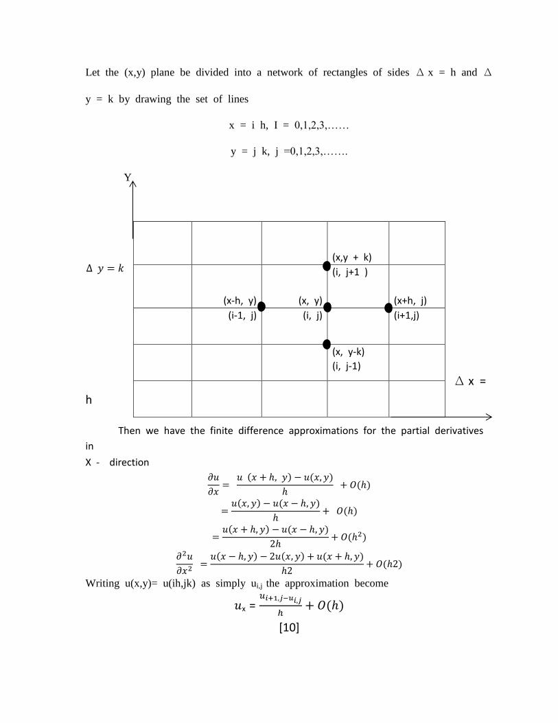
Let the (x,y) plane be divided into a network of rectangles of sides ∆ x = h and ∆

y = k by drawing the set of lines

x = i h, I = 0,1,2,3,……

y = j k, j =0,1,2,3,…….

Y

∆ x =

h

Then we have the finite difference approximations for the partial derivatives

in

X - direction

( ) ( )

( )

( ) ( )

( )

( ) ( )

( )

( ) ( ) ( )

( )

Writing u(x,y)= u(ih,jk) as simply ui,j the approximation become

x =

( )

[10]

(x,y + k)

(x-h, y)

(x, y)

(i, j+1 )

(x+h, j)

(i-1, j) (i, j) (i+1,j)

(x, y-k)

(i, j-1)

=

( )

u =

( )

and uxx =

( )

Similarly we have the approximations for the derivatives with respect to y.

=

( )

=

( )

=

( )

and uyy =

( )

We can use the following methods for iteration

(i) Jacobi’s method : Denoting the nth

derivative value of u(n)

i,j the iterative

formula to solve the partial differential equation is

It gives improved value of ui,j at the interior mesh points and is called the

point Jacobi’s formula.

(ii) Gauss – Seidal Method : In this method the iteration formula is

[11]

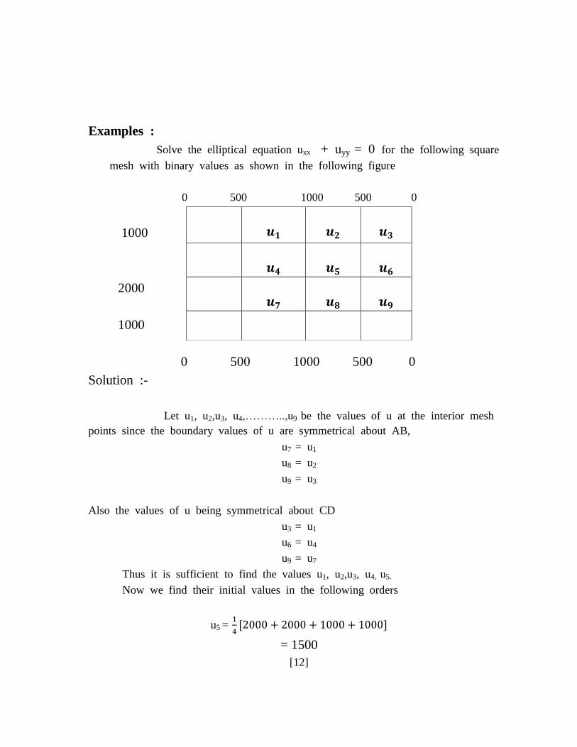
Examples :

Solve the elliptical equation uxx + uyy = 0 for the following square

mesh with binary values as shown in the following figure

0 500 1000 500 0

1000

2000

1000

0 500 1000 500 0

Solution :-

Let u1, u2,u3, u4,………..,u9 be the values of u at the interior mesh

points since the boundary values of u are symmetrical about AB,

u7 = u1

u8 = u2

u9 = u3

Also the values of u being symmetrical about CD

u3 = u1

u6 = u4

u9 = u7

Thus it is sufficient to find the values u1, u2,u3, u4, u5.

Now we find their initial values in the following orders

u5 =

= 1500

[12]

u1 =

= 1125

u2 =

(Standard Formula)

u4 =

(Standard Formula)

Now we carry out the iteration process using this standard formulae

u1 (n+1)

=

u2 (n+1)

=

u4 (n+1)

=

u5 (n+1)

=

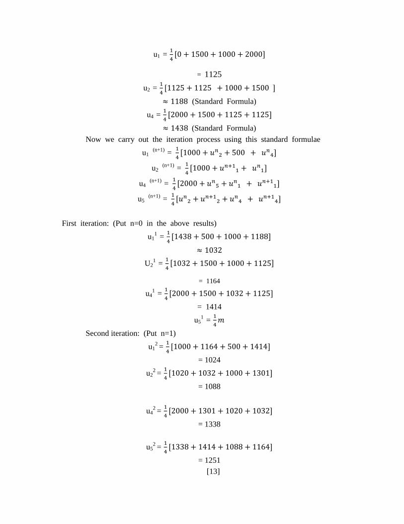
First iteration: (Put n=0 in the above results)

u11 =

U21

=

= 1164

u41 =

= 1414

u51 =

Second iteration: (Put n=1)

u12 =

= 1024

u22 =

= 1088

u42 =

= 1338

u52 =

= 1251

[13]

Third iteration: (Put n=2)

u13 =

= 982

u23 =

= 1063

u43 =

= 1313

u53 =

= 1201

Fourth iteration: (Put n=3)

u14 =

= 969

u24 =

= 1038

u44 =

= 1288

u54 =

= 1176

Fifth iteration: (Put n=4)

u15 =

= 957

u25 =

1026

u45 =

1276

u55 =

= 1157

Similarily

u16 = 951; u2

6 = 1016; u4

6 = 1266; u5

6 = 1146;

u17 = 946; u2

7 = 1011; u4

7 = 1260; u5

7 = 1138;

u18 = 943; u2

8 = 1007; u4

8= 1257; u5

8 = 1134;

u19 = 941; u2

9 = 1005; u4

9 = 1255; u5

9 = 1131;

[14]

u110

= 940; u210

= 1003; u410

= 1253; u510

= 1129;

u111

= 939; u211

= 1002; u411

= 1252; u511

= 1128;

u112 939; u2

12 1001; u412 1251; u5

12 1126;

There is negligible difference between the values obtained in the 11th

and 12th

iterations. Hence,

u1 = 939;

u2 = 1001;

u4 = 1251;

u5 = 1126;

Examples :

Given the values of u(x,y) on the boundary of the square in the

following figure evaluate the function u(x,y) satisfying the Laplace equation

at the pivotal points of the figure by a) Jacobi’s Method b) Gauss –

Seidal Method

Solution :-

Let u1, u2,u3, u4 be the initial values

We assume that u4 = 0; Then

u1 =

= 1000

u2 =

= 625(Standard Formula)

u3 =

(Standard Formula)

[15]

u1

u2

u3

u4

u4 =

(Standard Formula)

a) Now we carry out the successive iteration process using this Jacobi’s

formulae

u1 (n+1)

=

u2 (n+1)

=

u3 (n+1)

=

u4 (n+1)

=

First iteration: (Put n=0 in the above results)

u11 =

U21

=

u31 =

Second iteration : (Put n=1)

u12 =

= 1172

u22 =

= 750

u32 =

= 1000

u42 =

= 422

Similarly,

u13 1188; u2

3 774; u43 1024; u5

3 438;

u14 1200; u2

4 782; u44 1032; u5

4 450;

u15 1204; u2

5 788; u45 1038; u5

5 454;

u16 1206.5; u2

6 790; u46 1040; u5

6 456.5;

[16]

u17 1208; u2

7 791; u47 1041; u5

7 458;

u18 1208; u2

8 791.5; u48 1041.5; u5

8 458;

There is negligible difference between the values obtained in the 7h

and 8th

iterations. Hence,

u1 = 1208;

u2 = 792;

u4 = 1042;

u5 = 458;

b) We carry out the successive iterations, using Gauss-Seidal formulae

u1 (n+1)

=

u2 (n+1)

=

u3 (n+1)

=

u4 (n+1)

=

First iteration: (Put n=0 in the above results)

u11 =

u21 =

u31 =

u41 =

438

Second iteration : (Put n=1)

u12 =

u22 =

u32 =

[17]

u42 =

Similarly,

u13 1204; u2

3 789; u43 1040; u5

3 458;

u14 1207; u2

4 791; u44 1041; u5

4 458;

u15 1208; u2

5 791.5; u45 1041.5; u5

5 458.25;

There is negligible difference between the values obtained in the 4th

and 5th

iterations. Hence,

u1 = 1208;

u2 = 792;

u4 = 1042;

u5 = 458;

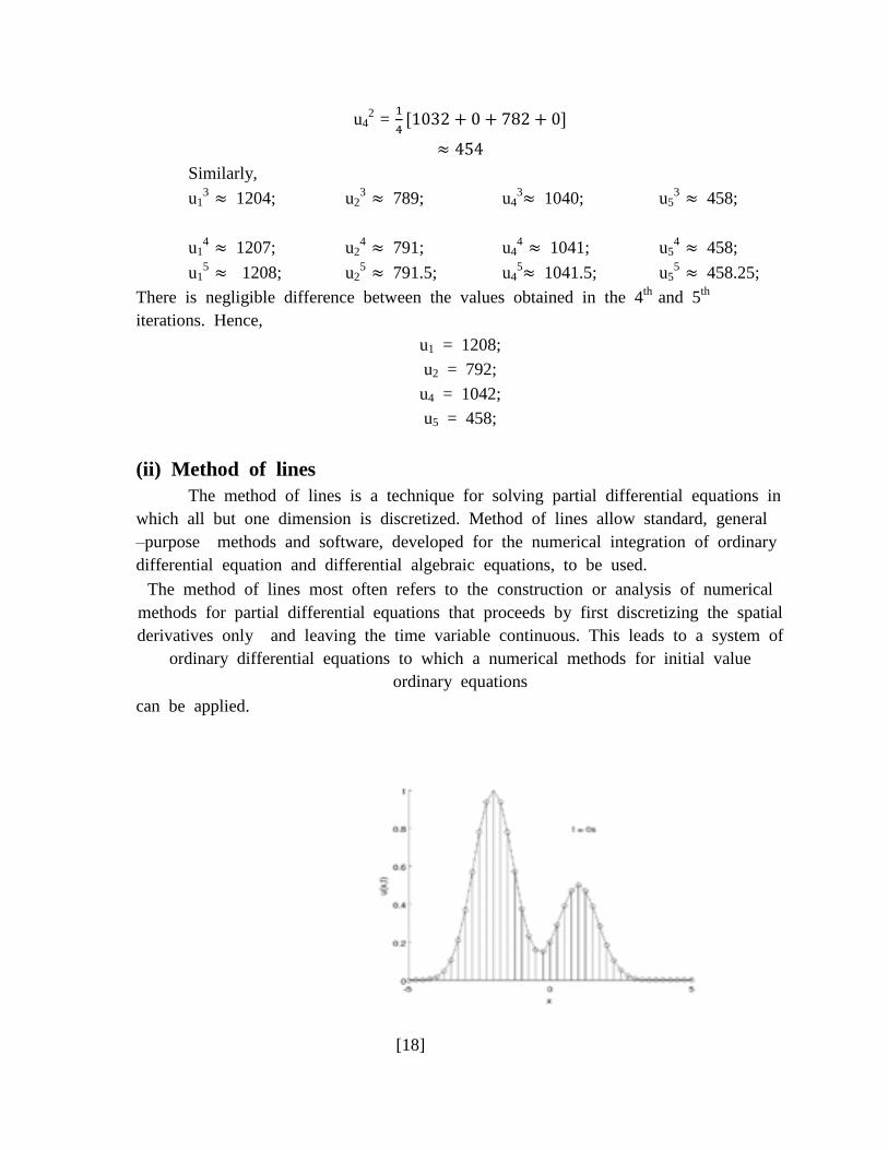
(ii) Method of lines

The method of lines is a technique for solving partial differential equations in

which all but one dimension is discretized. Method of lines allow standard, general

–purpose methods and software, developed for the numerical integration of ordinary

differential equation and differential algebraic equations, to be used.

The method of lines most often refers to the construction or analysis of numerical

methods for partial differential equations that proceeds by first discretizing the spatial

derivatives only and leaving the time variable continuous. This leads to a system of

ordinary differential equations to which a numerical methods for initial value

ordinary equations

can be applied.

[18]

(iii ) Domain decomposition methods

Domain decomposition method solve a boundary value problem by splitting it

into smaller boundary value problems on subdomains and iterating to coordinating

the solution between adjacent subdomains. A coarse problem with one or few

unknowns per sub domains is used to further coordinate the solutions between

the subdomains the subdomains globally. The domain problem on the subdomains

are independent , which make domain decomposition methods suitable for parallel

computing. Domain decomposition method is typically used as pre conditioners

for Krylo space iterative method , such as conjugate gradient method.

In overlapping domain decomposition methods , the subdomain overlapped by

more than the interface. Overlapping domain decomposition methods include the

Schwarz alternating method and additive Schwarz method. Many domain

decomposition methods can be written and analyzed as a special case of the

abstract additive Schwarz method

In non-overlapping domain decomposition methods the subdomains intersect

only on their interface. In primal methods, such as Balancing domain

decomposition and the continuity of the solution across subdomains interface is

enforced by representing the

value of the solution on all neighboring subdomains by the same unknowns. In

duel

method , the continuity of the solution across the subdomains interface is

enforced by Lagrange multipliers . Non-overlapping domain decomposition method

are also called iterative substructuring methods.

Domain decomposition methods embody large potential for a parallelization of

the finite element method , and serve a basis for distributed , parallel

computations.

[19]

Example :

u’’

(x) - u (x) = 0

u (0) = 0 ; u(1) = 1

The exact solution is:

u (x) = (ex - e

x) / (e

1 – e

-1)

Subdivide the domain into two subdomains, one from[0,1/2] and another from [1/2,1]. In

each of these two subdomains define interpolating functions v1(x)and v2(x)At the interface

between these two subdomains the following interface conditions shall be imposed:

v1(1/2) = v2(1/2)

v1’(1/2) = v2’(1/2)

Let the interpolating functions be defined as:

v1(x) = ∑ un Tn (y1(x))

v2(x) = ∑ un + N Tn (y2(x))

Where Tn (x) is the nth cardinal function of the Chebyshev polynomials of the first kind

with input argument y.

If N=4 then the following approximation is obtained by this scheme:

u1 = 0.6236

u2 = 0.21495

u3 = 0.37428

u4 = 0.44341

u5= 0.51492

u6 = 0.69972

u7 = 0.90645

(iv) Finite element method

The finite element method (FEM) is a numerical technique for finding approximate

solutions to boundary value problems for differential equations. It uses variational

methods (the calculus of variations) to minimize an error function and produce a

stable solution. Analogous to the idea that connecting many tiny straight lines can

approximate a larger circle, FEM encompasses all the methods for connecting many

simple element equations over many small subdomains, named finite elements, to

approximate a more complex equation over a larger domain.

[20]

2D finite element method, the triangles are the elements, the vertices are the nodes.

The finite element method (FEM) has been the tool of choice since its inception in

the 1940s for the simulation of structural mechanics. Today, the FEM is used to

model a much wider range of physical phenomena.

The extended finite element method (XFEM), also known as generalized finite

element method (GFEM) or partition of unity method (PUM) is a numerical

technique that extends the classical finite element method (FEM) approach by

enriching the solution space for solutions to differential equations with discontinuous

functions. The extended finite element method (XFEM) was developed in 1999 by

Ted Belytschko and collaborators,] to help alleviate shortcomings of the finite

element method and has been used to model the propagation of various

discontinuities: strong and weak (material interfaces). The idea behind XFEM is to

retain most advantages of meshfree methods while alleviating their negative sides.

The extended finite element method was developed to ease difficulties in

solving problems with localized features that are not efficiently resolved by mesh

refinement. One of the initial applications was the modeling of fractures in a

material. In this original implementation, discontinuous basis functions are added to

standard polynomial basis functions for nodes that belonged to elements that are

intersected by a crack to provide a basis that included crack opening displacements.

A key advantage of XFEM is that in such problems the finite element mesh does

not need to be updated to track the crack path. Subsequent research has illustrated

the more general use of the method for problems involving singularities, material

interfaces, regular meshing of microstructural features such as voids, and other

problems where a localized feature can be described by an appropriate set of basis

functions.

Enriched finite element methods extend, or enrich, the approximation space

so that it is able to naturally reproduce the challenging feature associated with the

problem of interest: the discontinuity, singularity, boundary layer, etc. It was shown

that for some problems, such an embedding of the problem's feature into the

approximation space can significantly improve convergence rates and accuracy.

Moreover, treating problems with

[21]

discontinuities with extended Finite Element Methods suppresses

the need to mesh and re mesh the discontinuity surfaces, thus alleviating the

computational costs and projection errors associated with conventional finite element

methods, at the cost of restricting the discontinuities to mesh edges.

Example:

Solving Poisson’s equation in one dimesion

-Uxx = q , 0 ≤ x ≤ L

using finite element method:

soln:

We consider Dirichlet boundary conditions:

U(0) = U(L) = 0.

A weak solution of - Uxx = q ,

considers the variational form of the above equation:

∫ ( ) ∫ ( )

( )

[22]

where (x) satisfy the boundary conditions:

(0) = (L) = 0.

We can integrate the first term by parts:

∫

( ) (x) ( ) } at x=0 to x =L

using ( ) ( ) .

Then ∫ ( ) ∫ ( )

( ) become ,

∫ ( ) ∫ ( )

( )

The above equation hold for all functions ( ) which are piece-wise continuous

and satisfies the bc : (0) = (L) = 0.

To solve equation

∫ ( ) ∫ ( )

( )

using the finite element method we again introduce a mesh on the interval [0, L]

with mesh points xj = j x , j = 0, . . . , n + 1 where, x =

.

To complete the discretisation we must choose a basis for (x).

The most common basis chosen for _(x) are the “hat” functions, j(x).

We solve ∫ ( ) ∫ ( )

( ) using these :

( ) ∑

( )

where,

( )

{

( )

( )

otherwise the value is zero.

with this construction :

( )

{

, zero otherwise..

[23]

We let (x) =∑ ( ) and (xi) = ai for i = 1, . . . , n, and (0) = ( )

= 0 and

( ) = (L) so that ( ) satisfies boundary conditions.

The hat functions are advantageous as a basis as they are nearly “orthonormal”,

ie , ∫ ( )

( )(x)dx = 0 when |j − k| > 1.

Using finite element method we seek an approximate solution which is satisfied

for

all basis functions, i(x), for i = 1, . . . , n:

∫ ( ) ∫ ( )

( )

; i=1,2,…..,n We

also expand the solution U(x) using the hat function as a basis :

U(x) =Uh(x)=∑ ( )

this simplifies our equation and we can solve for ; i=1,2,…..,n.

(v) Spectral Method

Spectral methods are a class of techniques used in applied mathematics and

scientific computing to numerically solve certain differential equations, often

involving the use of the Fast Fourier Transform. The idea is to write the solution of

the differential equation as a sum of certain "basis functions" (for example, as a

Fourier series which is a sum of sinusoids) and then to choose the coefficients in

the sum in order to satisfy the differential equation as well as possible.

Spectral methods and finite element methods are closely related and built on

the same ideas; the main difference between them is that spectral methods use basis

functions that are nonzero over the whole domain, while finite element methods use

basis functions that are nonzero only on small subdomains. In other words, spectral

methods take on a global approach while finite element methods use a local

approach. Partially for this reason, spectral methods have excellent error properties,

with the so-called "exponential convergence" being the fastest possible,

[24]

when the solution is smooth. However, there are no known three-dimensional

single domain spectral shock capturing results. In the finite element community, a

method where the degree of the elements is very high or increases as the grid

parameter h decreases to zero is sometimes called a spectral element method.

Spectral methods can be used to solve ordinary differential equations (ODEs),

partial differential equations (PDEs) and eigenvalue problems involving differential

equations. When applying spectral methods to time-dependent PDEs, the solution is

typically written as a sum of basis functions with time-dependent coefficients;

substituting this in the PDE yields a system of ODEs in the coefficients which can

be solved using any numerical method for ODEs. Eigenvalue problems for ODEs are

similarly converted to matrix eigenvalue problems.

Spectral methods were developed in a long series of papers by Steven Orszag

starting in 1969 including, but not limited to, Fourier series methods for periodic

geometry problems, polynomial spectral methods for finite and unbounded geometry

problems, pseudo spectral methods for highly nonlinear problems, and spectral

iteration methods for fast solution of steady state problems. The implementation of

the spectral method is normally accomplished either with collocation or a Galerkin

or a Tau approach.

Spectral methods are computationally less expensive than finite element

methods, but become less accurate for problems with complex geometries and

discontinuous coefficients. This increase in error is a consequence of the Gibbs

phenomenon.

Example :

Here we presume an understanding of basic multivariate calculus and Fourier

series. If g(x,y) is a known, complex-valued function of two real variables, and g is

periodic in x and y (that is, g(x,y)=g(x+2π,y)=g(x,y+2π)) then we are interested in

finding a function f(x,y) so that

(

+

)f(x,y) = g(x,y) for all x,y.

where the expression on the left denotes the second partial derivatives of f in x and

y, respectively. This is the Poisson equation, and can be physically interpreted as

some sort of heat conduction problem, or a problem in potential theory, among other

possibilities.

If we write f and g in Fourier series:

f = ∑ ( )

[25]

g =∑ ( )

and substitute in to the difference equation , obtain this equation :

We have exchanged partial differentiation with an infinite sum, which is

legitimate if we assume for instance that f has a continuous second derivative. By

the uniqueness theorem for Fourier expansions, we must then equate the Fourier

coefficients term by term, giving

which is an explicit formula for the Fourier coefficients aj,k.

With periodic boundary conditions, the Poisson equation possesses a solution

only if b0,0 = 0. Therefore we can freely choose a0,0 which will be equal to the

mean of the resolution. This corresponds to choosing the integration constant.

To turn this into an algorithm, only finitely many frequencies are solved for.

This introduces an error which can be shown to be proportional to , where

and is the highest frequency treated.

(vi) Mesh Free Methods

In the field of numerical simulation methods, meshfree methods are those that do not

require that a mesh connect data points of the simulation domain. Meshfree methods enable

the simulation of some otherwise difficult types of problems, at the cost of extra computing

time and programming effort.

Numerical methods such as the finite difference method, finite-volume method, and

finite element method were originally defined on meshes of data points. In such a mesh,

each point has a fixed number of predefined neighbors, and this connectivity between

neighbors can be used to define mathematical operators like the derivative. These operators

are then used to construct the equations to simulate—such as the Euler equations or the

Navier–Stokes equations.But in simulations where the material being simulated can move

around (as in computational fluid dynamics) or where large deformations of the material can

occur (as in simulations of plastic materials), the connectivity of the mesh can be difficult to

maintain without

[26]

introducing error into the simulation. If the mesh becomes tangled or degenerate during

simulation, the operators defined on it may no longer give correct values. The mesh may be

recreated during simulation (a process called remeshing), but this can also introduce error,

since all the existing data points must be mapped onto a new and different set of data points.

Meshfree methods are intended to remedy these problems. Nodal integration has been

proposed as a technique to use finite elements to emulate a meshfree behaviour.[1]

However,

the obstacle that must be overcome in using nodally integrated elements is that the quantities

at nodal points are not continuous, and the nodes are shared among multiple elements.

Meshfree methods are also useful for:

Simulations where creating a useful mesh from the geometry of a complex 3D object

may be especially difficult or require human assistance

Simulations where nodes may be created or destroyed, such as in cracking

simulations

Simulations where the problem geometry may move out of alignment with a fixed

mesh, such as in bending simulations

Simulations containing nonlinear material behavior, discontinuities or singularities

Example

In a traditional finite difference simulation, the domain of a one-dimensional

simulation would be some function u (x,t), represented as a mesh of data values uin

at points

xi, where

I = 0,1,2,………………….

n = 0,1,2,…………………

xn+1 -xi = h for every i

tn+1-tn = k for every k

We can define the derivatives that occur in the equation being simulated using some

finite difference formulae on this domain, for example

(ui+1

n _ ui-1

n )/ 2h

and

= (ui

n+1 – ui-1

n) / k

Then we can use these definitions of u (x,t) and its spatial and temporal derivatives

to write the equation being simulated in finite difference form, then simulate the equation

[27]

with one of many finite difference methods.

In this simple example, the spatial step size h and the temporal step size kare

constant, and the left and right mesh neighbors of the data value at are the values at

xi-1and xi+1 , respectively. But if the values can move around, or can be added to or removed

from the simulation, that destroys the spacing and the simple finite difference formulae for

derivatives is no longer correct.

Smoothed-particle hydrodynamics (SPH), one of the oldest meshfree methods,

solves this problem by treating data points as physical particles with mass and density that

can move around over time, and carry some value with them. SPH then defines the value

of u (x,t)between the particles by

u (x,t) = ∑ mi (uin/ϸi) W (/x - xi/)

where mi is the mass of particle , is the density of particle i , and W is a kernel function

that operates on nearby data points and is chosen for smoothness and other useful qualities.

By linearity, we can write the spatial derivative as

∑ mi (ui

n/ϸi)

W (/x - xi/)

Then we can use these definitions of u (x,t) and its spatial derivatives to write the

equation being simulated as an ordinary differential equation, and simulate the equation with

one of many numerical methods. In physical terms, this means calculating the forces

between the particles, then integrating these forces over time to determine their motion.

The advantage of SPH in this situation is that the formulae for u (x,t) and its

derivatives do not depend on any adjacency information about the particles; they can use the

particles in any order, so it doesn't matter if the particles move around or even exchange

places.

One disadvantage of SPH is that it requires extra programming to determine the

nearest neighbors of a particle. Since the kernel function W only returns nonzero results for

nearby particles within twice the "smoothing length" (because we typically choose kernel

functions with compact support), it would be a waste of effort to calculate the summations

above over every particle in a large simulation. So typically SPH simulators require some

extra code to speed up this nearest neighbor calculation.

(vii) Multigrid method

Multigrid (MG) methods in numerical analysis are a group of algorithms for solving

differential equations using a hierarchy of discretizations. They are an example of a class of

techniques called multiresolution methods,

[28]

very useful in (but not limited to) problems exhibiting multiple scales of behavior.

For example, many basic relaxation methods exhibit different rates of convergence

for short- and long-wavelength components, suggesting these different scales be treated

differently, as in a Fourier analysis approach to multigrid. MG methods can be used as

solvers as well as preconditioners.

The main idea of multigrid is to accelerate the convergence of a basic iterative

method by global correction from time to time, accomplished by solving a coarse problem.

This principle is similar to interpolation between coarser and finer grids. The typical

application for multigrid is in the numerical solution of elliptic partial differential equations

in two or more dimensions.

Multigrid methods can be applied in combination with any of the common

discretization techniques. For example, the finite element method may be recast as a

multigrid method. In these cases, multigrid methods are among the fastest solution

techniques known today. In contrast to other methods, multigrid methods are general in that

they can treat arbitrary regions and boundary conditions. They do not depend on the

separability of the equations or other special properties of the equation. They have also been

widely used for more-complicated non-symmetric and nonlinear systems of equations, like

the Lamé system of elasticity or the Navier-Stokes equations.

There are many variations of multigrid algorithms, but the common features are that a

hierarchy of discretizations (grids) is considered. The important steps are

Smoothing – reducing high frequency errors, for example using a few iterations of

the Gauss–Seidel method.

Restriction – downsampling the residual error to a coarser grid.

Interpolation or prolongation – interpolating a correction computed on a coarser grid

into a finer grid.

A multigrid method with an intentionally reduced tolerance can be used as an

efficient preconditioner for an external iterative solver. The solution may still be

obtained in O (N) time as well as in the case where the multigrid method is used as a

solver. Multigrid preconditioning is used in practice even for linear systems. Its main

advantage versus a purely multigrid solver is particularly clear for nonlinear

problems, e.g., eigenvalue problems.

Generalized multigrid methods

Multigrid methods can be generalized in many different ways. They can be applied

naturally in a time-stepping solution of parabolic partial differential equations, or

they can be applied directly to time-dependent partial differential equations.

Research on multilevel techniques for hyperbolic partial differential equations is

underway.

[29]

Multigrid methods can also be applied to integral equations, or for problems in

statistical physics.

Other extensions of multigrid methods include techniques where no partial

differential equation nor geometrical problem background is used to construct the

multilevel hierarchy. Such algebraic multigrid methods (AMG) construct their

hierarchy of operators directly from the system matrix, and the levels of the

hierarchy are simply subsets of unknowns without any geometric interpretation.

Thus, AMG methods become true black-box solvers for sparse matrices. However,

AMG is regarded as a

dvantageous mainly where geometric multigrid is too difficult to apply.

Another set of multiresolution methods is based upon wavelets. These wavelet

methods can be combined with multigrid methods. For example, one use of wavelets

is to reformulate the finite element approach in terms of a multilevel method.

Adaptive multigrid exhibits adaptive mesh refinement, that is, it adjusts the grid as

the computation proceeds, in a manner dependent upon the computation itself. The

idea is to increase resolution of the grid only in regions of the solution where it is

needed.

[30]

CHAPTER 4

APPLICATIONS

Mathematical Models For Oil Reservoir Simulation

Flow Model

The second part of a reservoir model is a mathematical model that describe

the fluid flow. In the following we will describe the most common model are

isothermal flow. For brevity, we do not discuss thermal and coupled geomechanical

fluid models even though these are sometimes necessary to reprasent first order

effects.

Single Phase Flow

The flow of a single fluid with density through a porous medium

described using the fundamental property of conservation of mass.

( )

( ) …………………….(1)

Here v is the superficial velocity and q denotes a fluid force or sink term

used to model wells. The velocity is related to the fluid pressure , p through an

empirical relation named the French engineer , Henri Darcy:

( ) …………………(2)

Where k is the permeability, the fluid velocity, and g the gravity vector,

introducing rock and fluid compressibilities cr =

and c =

(1) and (2) can

be combined to a parabolic equation for the fluid pressure.

( ) ( )

(

( )) = q …………………..(3)

In the special case of incompressible rock and fluid (3) simplifies to a Poison

equation with variable coefficients. - ( ) =

, for the fluid potential

z .

[31]

Two Phase Flow

The void space in a reservoir will generally be filled by hydrocarbons and

(salt) water . In addition , water is frequently injected to improve hydrocarbon

recovery. If the fluids are immiscible and separated by a sharp interface, they are

referred to as phases. A two phase system is commonly divided into a wetting and

non-wetting phase , given by the contact angle between the solid surface and the

fluid-fluid interface on the microscale (Acute angle implies wetting phase ). On the

macroscale, the fluids are assumed to be present at the same location, and the

volume fraction occupied by each phase is called the saturation of that phase ; For a

two phase system the saturation of the wetting and non-wetting phases therefore

sum to unity Sn+Sw = 1.

In the absence of phase transitions , the saturation change when on phase

displaces the other . During the displacement , the ability of one phase to move is

affected by the interaction with the other phase at the pore scale . In the

microscopic mode l, this affect is represented by the relative permeability krɑ (ɑ = w ,

n) , which is a dimensionless scaling factor that depends on the saturation and

modifies the absolute permeability to account for the rock’s reduced ability to

transmit each fluid in the presence of the other . The multi-phase extension of

Darcy’s law reads

( ) q …………………..(4)

which together with the mass conservation of each phase

( )

+ ( ) ( ) …………………………..(5)

forms the basic equation because of interfacial tension, the pressure in the two face

will differ . The pressure difference is called capillary pressure pcnw = pn - pw and is

usually assumed to be a function of saturation on macro scale .

To better reveal the nature of mathematical model , it is common to

reformulate (4) and (5) as a flow equation for fluid pressure and transport equation

for saturation . A straight forward manipulation leads to a system for one phase

pressure and one saturation in which the capillary pressure appears explicitly . The

resulting equations are nonlinear and strongly coupled. To reduce the coupling , one

can introduce a global pressure , p = pn – pc where we complementary pressure

contains the saturation dependent terms and is defined as . The

dimensionless fractional flow functions fw = ʎw + (ʎw + ʎn) measures the fraction of the

total flow that contains the wetting phase and is defined from the phase mobilities

ʎ . . In the compressible and immiscible case , (4) and (5) can now be

written in the so-called fractional form which consist of an elliptic pressure equation

( ) ( ) ……………(6)

[32]

for the pressure and the total velocity v = vn + vw and a parabolic saturation equation.

( ) ( ) )

…………………(7)

For the saturation Sw of the wetting phase . The capillary pressure can often be

neglected on a sufficiently large scale in which case (7) becomes hyperbolic .

To solve the system (6) and (7) numerically , it common to use a sequencial

solution .

First (6) is solved to determine the pressure and velocity , which are then held fixed

while advancing the saturation a time step , and so on.

Multiphase , Multicomponent flow

Extending the equations describing two phase flow to immiscible flow of more

than two phases is straight forward mathematically, but defining parameters such as

relative permeability becomes more challenging . In addition, each phase will consist

of more than one chemical species , which are typically grouped into fluid

components because fluid components may transfer between phases (and change

compositions ), the basic conservation laws are expressed for each component l,

( ∑ ) (∑ ) = ∑ ……………………..(8)

Here denotes the mass fraction of component l in phase is the

density of phase is phase velocity, and q is phase source . As above, the

velocities are modelled using the multiphase extension of Darci’s law (4) . The

system consisting of (8) and (4) is just the starting point of modeling and must be

further manipulated and supplied with closure relations (PVT models , phase

equilibrium conditions , etc .) for specific fluid systems . Different choices for closure

relationships are appropriate for different reservoir and different recovery mechanisms

and lead to different levels of model complexity .

The Black-oil Model

The flow model that is used most within reservoir simulation is the black oil

model. The model uses a simple PVT description in which the hydrocarbon chemical

species are lumped together to form two components at surface conditions: a heavy

hydrocarbon called “oil” and a light hydrocarbon component “gas”, for which the

chemical composition to remain constant for all times . at reservoir conditions the gas

component may be partially or completely dissolved in the oil phase , forming one or

two phases(liquid and vapour) that do not dissolve in the water phase. In more

general models , oil can be dissolved in the gas phase, the hydrocarbon component

are allowed to be dissolved in the water (aquous) phase,

[33]

and the water component may be dissolved in the two hydrocarbon phases.

The black oil model is often formulated as conservation of volumes at

standard conditions rather than conservation of component masses by introducing

formation volume factors B = V (V are volumes occupied by a

bulk of component at reservoir and surface conditions) and a gas solubility factor

, which is the volume of gas, measured at a standard conditions, dissolved

at reservoir conditions in a unit of stock-tank oil (at surface condition). The

resulting conservation laws read

(

) +

,

(

)

+

, ……………………..(10)

Commercial simulators typically use a fully implicit discretization to solve the

non-linear system (9). However, there are also several sequential methods that vary in

the choice of primary unknowns and the manipulations, linearization, temporal and

spatial discretization, and the order in which these operations are applied to derive a

set of discrete equation. As an example, the implicit pressure and explicit saturation

method starts by a temporal discretization of balance equations (9) and then eliminates

the volume factors to derive a pressure equation that is solved implicitly to obtain

pressure and fluxes. These are then used to update the volumes (or saturations) in an

explicit time step. Improved stability can be obtained by a sequential implicit method

that also treats the saturation equation implicitly.

[34]

BIBLIOGRAPHY

Textbooks -

Introductory Methods of Numerical Analysis ------------

S.S Sastry

Numerical Methods in Engineering and Science ------------

Dr. B.S. Grewal

Numerical solution of partial differential equations ------------

Dr. Louise Olsen-Kettle

Numerical solution of partial differential equations ------------

Gordon C. Everstine

Internet –

Wikipedia – Free Encyclopedia

Britannica - Online Encyclopedia

Google – Search Engine

[35]