Embed Size (px)
Citation preview
Slot car hardware assembling, localization and reinforcementlearning on a Carrera132 track
Final year project
Author:Jesu Lago GarciaAlfonso Lima Astor
Supervisor:Prof. Dr. Wolfram Burgard
Prof. Dr. Rafael Sanz DominguezMr. Lucas Chiesa
Subbmited on: July 2013


AbstractLocalization and self-learning are fundamental demands among robots. In this project,we present a new model for slot car localization and self-learning speed planning in adiscrete environment made up by a Carrera132 race track. In our approach, we haveselected and assembled onto the car the hardware equipment required to: first, createa motion model based on the linear and angular car speeds, working in tandem with amodel for car positioning based on the recognition of track pieces using tags. Secondly,communicate the car with a computer which is responsible for the car localization, thespeed planning and high level application. Thanks to this equipment, we could createfor the car localization a Particle Filter, which uses not only the regular sensor measures,but also the geometry of the track in the update step. Moreover, since we based the speedplanning task on a reinforcement learning application which need the car position to developthe speed planning, the Particle Filter was able to provide this requirement. Finally, all theprocesses for this tasks has been done using ROS, and a complete simulation of the track,the car position and the Particle filter was created within the RVIZ software.


Acknowledgement
We would like to thank everybody who has supported our work, especially our supervisorsProf. Dr. Wolfram Burgard, Prof. Dr. Rafael Sanz Dominguez, and Lucas Chiesa for theabsorbing topic and all the ideas and help which they have provided. In addition, we alsowant to thank all the people of the "Autonomous Intelligent Systems" group in Freiburg,particularly Ramin Zohouri for his help on machine learning and to Bahran Behzadian forhis clarifications on robot localization. Finally, we would also like to show our gratitude toour family, who has always encourage us to persist in our work.
3

CONTENTS
Contents
1 Introduction 12
1.1 Goal . . . . . . . . . . . . . . . . . . . . . . . . . . . . . . . . . . . . . . . . 12
2 Project planning 15
3 Resources selection 17
4 Hardware 19
4.1 Voltage Regulator - Texas Instrument PTN78000W . . . . . . . . . . . . . . 19
4.1.1 General description . . . . . . . . . . . . . . . . . . . . . . . . . . . . 19
4.1.2 Electrical Specifications . . . . . . . . . . . . . . . . . . . . . . . . . 20
4.1.3 Application circuit . . . . . . . . . . . . . . . . . . . . . . . . . . . . 20
4.1.4 Specific use in the project . . . . . . . . . . . . . . . . . . . . . . . . 21
4.1.5 Power supply connection schematic . . . . . . . . . . . . . . . . . . . 21
4.2 Baby Orangutan B-328 controller . . . . . . . . . . . . . . . . . . . . . . . . 22
4.2.1 General description . . . . . . . . . . . . . . . . . . . . . . . . . . . . 22
4.2.2 Module pinout and component identification . . . . . . . . . . . . . . 22
4.2.3 Schematic . . . . . . . . . . . . . . . . . . . . . . . . . . . . . . . . . 24
4.2.4 General specifications . . . . . . . . . . . . . . . . . . . . . . . . . . 26
4.2.5 ATmega 328P microcontroller . . . . . . . . . . . . . . . . . . . . . . 26
4.2.6 TB6612FNG dual H-bridge . . . . . . . . . . . . . . . . . . . . . . . 28
4.2.7 Specific use in this project . . . . . . . . . . . . . . . . . . . . . . . . 29
5

CONTENTS
4.3 QTR-8RC Reflectance Sensor Array . . . . . . . . . . . . . . . . . . . . . . 29
4.3.1 General description . . . . . . . . . . . . . . . . . . . . . . . . . . . . 29
4.3.2 Electrical and optical specifications . . . . . . . . . . . . . . . . . . . 31
4.3.3 Output behavior . . . . . . . . . . . . . . . . . . . . . . . . . . . . . 32
4.3.4 Breaking the sensor in 2 modules . . . . . . . . . . . . . . . . . . . . 33
4.3.5 Specific use in the project . . . . . . . . . . . . . . . . . . . . . . . . 33
4.3.6 Connection schematic . . . . . . . . . . . . . . . . . . . . . . . . . . 34
4.4 Distance measuring optoelectronic sensor Sharp GP2D120 . . . . . . . . . . 35
4.4.1 General description . . . . . . . . . . . . . . . . . . . . . . . . . . . . 35
4.4.2 Electrical and electrooptical Specifications . . . . . . . . . . . . . . . 35
4.4.3 Output behavior . . . . . . . . . . . . . . . . . . . . . . . . . . . . . 36
4.4.4 Specific use in the project . . . . . . . . . . . . . . . . . . . . . . . . 36
4.4.5 Connection schematic . . . . . . . . . . . . . . . . . . . . . . . . . . 38
4.5 Hall effect sensor - Melexis US1881 . . . . . . . . . . . . . . . . . . . . . . . 39
4.5.1 General description . . . . . . . . . . . . . . . . . . . . . . . . . . . . 39
4.5.2 Electrical and Magnetical Specifications . . . . . . . . . . . . . . . . 40
4.5.3 Output Behaviour versus Magnetic Pole . . . . . . . . . . . . . . . . 40
4.5.4 Application circuit . . . . . . . . . . . . . . . . . . . . . . . . . . . . 40
4.5.5 Specific use in the project . . . . . . . . . . . . . . . . . . . . . . . . 42
4.5.6 Connection schematic . . . . . . . . . . . . . . . . . . . . . . . . . . 42
4.6 IMU - MinIMU-9 v2 . . . . . . . . . . . . . . . . . . . . . . . . . . . . . . . 43
4.6.1 General description . . . . . . . . . . . . . . . . . . . . . . . . . . . . 43
6

CONTENTS
4.6.2 Technical Specifications and Pin Description . . . . . . . . . . . . . . 44
4.6.3 TWI protocol . . . . . . . . . . . . . . . . . . . . . . . . . . . . . . . 44
4.6.4 Specific use in the project . . . . . . . . . . . . . . . . . . . . . . . . 48
4.6.5 Connection schematic . . . . . . . . . . . . . . . . . . . . . . . . . . 50
4.7 Wixel Programmable USB Wireless Module . . . . . . . . . . . . . . . . . . 51
4.7.1 General description . . . . . . . . . . . . . . . . . . . . . . . . . . . . 51
4.7.2 Module pinout and component identification . . . . . . . . . . . . . . 51
4.7.3 Schematic . . . . . . . . . . . . . . . . . . . . . . . . . . . . . . . . . 53
4.7.4 General specifications . . . . . . . . . . . . . . . . . . . . . . . . . . 53
4.7.5 Specific use in the project . . . . . . . . . . . . . . . . . . . . . . . . 53
4.7.6 Connection schematic . . . . . . . . . . . . . . . . . . . . . . . . . . 57
4.8 Printed circuit board (PCB) . . . . . . . . . . . . . . . . . . . . . . . . . . . 57
4.8.1 General description . . . . . . . . . . . . . . . . . . . . . . . . . . . . 57
4.8.2 Secondary PCB . . . . . . . . . . . . . . . . . . . . . . . . . . . . . . 58
4.9 Board for switch management . . . . . . . . . . . . . . . . . . . . . . . . . . 58
4.9.1 General description . . . . . . . . . . . . . . . . . . . . . . . . . . . . 58
4.9.2 Hardware required . . . . . . . . . . . . . . . . . . . . . . . . . . . . 58
4.9.3 Connection schematic . . . . . . . . . . . . . . . . . . . . . . . . . . 62
4.9.4 Specific use in the project . . . . . . . . . . . . . . . . . . . . . . . . 62
5 Car packed and track pieces identification 65
5.1 Car assembled . . . . . . . . . . . . . . . . . . . . . . . . . . . . . . . . . . . 65
5.2 World model - track pieces identification . . . . . . . . . . . . . . . . . . . . 66
7

CONTENTS
6 Project communications 70
6.1 General description . . . . . . . . . . . . . . . . . . . . . . . . . . . . . . . . 70
6.2 Protocol definition . . . . . . . . . . . . . . . . . . . . . . . . . . . . . . . . 70
6.2.1 Packet syntax . . . . . . . . . . . . . . . . . . . . . . . . . . . . . . . 70
6.2.2 Packet encoding . . . . . . . . . . . . . . . . . . . . . . . . . . . . . 71
6.2.3 Control bytes . . . . . . . . . . . . . . . . . . . . . . . . . . . . . . . 71
6.3 Data flow direction . . . . . . . . . . . . . . . . . . . . . . . . . . . . . . . . 73
6.4 Serial channel communication . . . . . . . . . . . . . . . . . . . . . . . . . . 73
6.5 Wixels Communication . . . . . . . . . . . . . . . . . . . . . . . . . . . . . . 75
6.6 USB communication . . . . . . . . . . . . . . . . . . . . . . . . . . . . . . . 75
6.7 Orders . . . . . . . . . . . . . . . . . . . . . . . . . . . . . . . . . . . . . . . 75
7 Low level programming 78
7.1 Low level libraries definition . . . . . . . . . . . . . . . . . . . . . . . . . . . 78
7.1.1 Array.c . . . . . . . . . . . . . . . . . . . . . . . . . . . . . . . . . . 78
7.1.2 Status_control.c . . . . . . . . . . . . . . . . . . . . . . . . . . . . . 79
7.1.3 Control.c . . . . . . . . . . . . . . . . . . . . . . . . . . . . . . . . . 80
7.1.4 Eeprom.c . . . . . . . . . . . . . . . . . . . . . . . . . . . . . . . . . 81
7.1.5 IMU.c . . . . . . . . . . . . . . . . . . . . . . . . . . . . . . . . . . . 82
7.1.6 Main.c . . . . . . . . . . . . . . . . . . . . . . . . . . . . . . . . . . . 84
7.1.7 Motor.c . . . . . . . . . . . . . . . . . . . . . . . . . . . . . . . . . . 86
7.1.8 PID.c . . . . . . . . . . . . . . . . . . . . . . . . . . . . . . . . . . . 86
8
CONTENTS
7.1.9 Sharp.c . . . . . . . . . . . . . . . . . . . . . . . . . . . . . . . . . . 87
7.1.10 Serial.c . . . . . . . . . . . . . . . . . . . . . . . . . . . . . . . . . . 87
7.1.11 Track.c . . . . . . . . . . . . . . . . . . . . . . . . . . . . . . . . . . 87
8 PID designing and programming 88
8.1 PID designing . . . . . . . . . . . . . . . . . . . . . . . . . . . . . . . . . . . 88
8.2 PID testing . . . . . . . . . . . . . . . . . . . . . . . . . . . . . . . . . . . . 90
9 High level for serial communication and debugging purpose 92
9.1 Glade software . . . . . . . . . . . . . . . . . . . . . . . . . . . . . . . . . . 92
9.2 ROS software . . . . . . . . . . . . . . . . . . . . . . . . . . . . . . . . . . . 92
9.3 Computer serial communication - SerialCom Node . . . . . . . . . . . . . . 93
9.3.1 Data reception . . . . . . . . . . . . . . . . . . . . . . . . . . . . . . 94
9.3.2 Data sending . . . . . . . . . . . . . . . . . . . . . . . . . . . . . . . 95
9.3.3 Buffers management . . . . . . . . . . . . . . . . . . . . . . . . . . . 95
9.4 High level application . . . . . . . . . . . . . . . . . . . . . . . . . . . . . . 96
9.5 Data debug . . . . . . . . . . . . . . . . . . . . . . . . . . . . . . . . . . . . 96
9.5.1 Accelerometer debug . . . . . . . . . . . . . . . . . . . . . . . . . . . 99
9.5.2 Magnetometer debug . . . . . . . . . . . . . . . . . . . . . . . . . . . 101
10 RVIZ simulation implementation 103
10.1 General overview . . . . . . . . . . . . . . . . . . . . . . . . . . . . . . . . . 103
10.2 Project elements design . . . . . . . . . . . . . . . . . . . . . . . . . . . . . 103
9
CONTENTS
11 Track Node 107
11.1 Track representation on RVIZ . . . . . . . . . . . . . . . . . . . . . . . . . . 107
11.2 Piece positions calculation . . . . . . . . . . . . . . . . . . . . . . . . . . . . 107
12 Particle filter design and implementation 109
12.1 Localization filter evaluation . . . . . . . . . . . . . . . . . . . . . . . . . . . 109
12.2 Particle Filter definition . . . . . . . . . . . . . . . . . . . . . . . . . . . . . 109
12.3 Particle filter design . . . . . . . . . . . . . . . . . . . . . . . . . . . . . . . 111
12.3.1 Number of particles . . . . . . . . . . . . . . . . . . . . . . . . . . . 112
12.3.2 Position propagation-update step . . . . . . . . . . . . . . . . . . . . 113
12.3.3 Angular speed propagation-update step . . . . . . . . . . . . . . . . 115
12.3.4 Resampling and Random Particles . . . . . . . . . . . . . . . . . . . 116
12.3.5 Localization of the car . . . . . . . . . . . . . . . . . . . . . . . . . . 117
12.4 Particle filter test and simulation . . . . . . . . . . . . . . . . . . . . . . . . 118
13 Artificial Intelligence implementation 119
13.1 MDP and Reinforcement Learning algorithm . . . . . . . . . . . . . . . . . 119
13.2 Project implementation . . . . . . . . . . . . . . . . . . . . . . . . . . . . . 120
13.3 New Q-States Exploration . . . . . . . . . . . . . . . . . . . . . . . . . . . . 122
13.4 MDP testing . . . . . . . . . . . . . . . . . . . . . . . . . . . . . . . . . . . 124
13.5 Learning extrapolation . . . . . . . . . . . . . . . . . . . . . . . . . . . . . . 124
14 ROS nodes interconnection 126
10

CONTENTS
15 Main drawbacks of our model 128
16 Conclusion and summary 130
17 Flow diagrams 131
17.1 Low level . . . . . . . . . . . . . . . . . . . . . . . . . . . . . . . . . . . . . 131
17.1.1 Main.c . . . . . . . . . . . . . . . . . . . . . . . . . . . . . . . . . . . 131
17.1.2 Array.c . . . . . . . . . . . . . . . . . . . . . . . . . . . . . . . . . . 136
17.1.3 Status_control.c . . . . . . . . . . . . . . . . . . . . . . . . . . . . . 138
17.1.4 Control.c . . . . . . . . . . . . . . . . . . . . . . . . . . . . . . . . . 140
17.1.5 Eeprom.c . . . . . . . . . . . . . . . . . . . . . . . . . . . . . . . . . 144
17.1.6 IMU.c . . . . . . . . . . . . . . . . . . . . . . . . . . . . . . . . . . . 148
17.1.7 Motor.c . . . . . . . . . . . . . . . . . . . . . . . . . . . . . . . . . . 151
17.1.8 PID.c . . . . . . . . . . . . . . . . . . . . . . . . . . . . . . . . . . . 152
17.1.9 Sharp.c . . . . . . . . . . . . . . . . . . . . . . . . . . . . . . . . . . 154
17.1.10Serial.c . . . . . . . . . . . . . . . . . . . . . . . . . . . . . . . . . . 155
17.1.11Track.c . . . . . . . . . . . . . . . . . . . . . . . . . . . . . . . . . . 162
17.2 High level . . . . . . . . . . . . . . . . . . . . . . . . . . . . . . . . . . . . . 163
17.2.1 Track node . . . . . . . . . . . . . . . . . . . . . . . . . . . . . . . . 163
17.2.2 Particle Filter node . . . . . . . . . . . . . . . . . . . . . . . . . . . . 164
17.2.3 MDP node . . . . . . . . . . . . . . . . . . . . . . . . . . . . . . . . 165
11

1 Introduction
From the first localization methods using start positions to the modern tools such GPS,and from the old learning processes such as the language acquisition to the current advanceresearches in science, it seems that throughout human history self-localization and self-learning has been primordial task. Therefore, it seems reasonable that both capabilitiesshould be implemented in robots in order to make them able to performance human tasks.
1.1 Goal
In this project, the main goal was the implementation of both abilities in a small slot car,which races in a Carrera track. Carrera is a slot track brand, which has several sort of slotcar tracks with different features. Concretely, we had to build the autonomous slot car forthe specific track Carrera 132. The figure picture 1 on page 12 illustrates an example of aCarrera 132 track.
Figure 1: Carrera 132 track illustration
12

1 INTRODUCTION
Starting with a slot car, we unmount the whole car, remaining only the chassis and themotor, so that selecting the appropriate hardware to implement the control of the car speedand to build a localization filter, we assembled the hardware in the car and we programit in order to make it send all the sensor data to a computer. This computer had to takecare of the localization filter, a High Level application in order to communicate with thecar, and an Artificial Intelligence that made the car learn by itself the optimum speeds inthe different parts of the circuit. The figure picture 2 on page 14 shows the car before andafter being unmounted and assembled whit the specific hardware.
The project duration was 9 months, and the different processes as well as the project planingwill be described in the next sections.
13

1.1 Goal
(a) Initial slot car before being unmounted
(b) Final slot car after being assembled
Figure 2: Slot car initial and final state
14

2 Project planning
The picture 3 on page 15 and the picture 4 on page 16 illustrates the final project planning,which specifies the different steps of the project, as well as the time required for each oneof those stages.
Figure 3: First months project planning
15

Figure 4: Last months project planning
16

3 Resources selection
In order to select the hardware equipment, we considered the final goals. Therefore, sincethe main final goal was the car localization, the self-learning speed and the wireless com-munication with the computer, we thought that the car needed the the following hardware:
1. An inertial measurement unit (IMU), so that we could have the measurements ofacceleration and angular speed in order to create the car motion model in the local-ization filter. The resource selected is explained in the section 4.6.
2. A encoder, which could give us the car speed reading the angular speed of the carwheels. The selection and construction of this encoder was done sticking magnets tothe wheel, and using a Hall sensor in order to read the magnetic pulses. This sensoris explained in the section 4.5.
3. A infrared optical sensor in order to read bar codes along the track. The specificationsof this sensor are explained in the section 4.3.
4. A distance measurement sensor so as to detect the presence of other slot cars in frontof our car, as well as the distance to those cars. The resource selected is explained inthe section 4.4.
5. A main microcontroller, whose chief task is taking care of the configuration/ reading/writing of the several sensors, as well as the car speed control. This microcontrolleris explained in the section 4.2.
6. A second microcontroller, which establishes wireless communication with the com-puter. This second microntroller is required because despite that we try to find apowerful microcontroller with wireless communication and small size, we could notfind it, therefore, we had to implement a small powerful microncontroller for the maintasks, and this second one just for the communications. This resource is explained inthe section 4.7.
7. A voltage regulator in order to adapt the track power to the power required forthe hardware equipment. The specifications of this regulator are illustrated in thesection 4.1.
17

8. A small circuit with a reed switch, a microcontroller and with USB connection withthe computer, which manages the side switches of the track. The specifications ofthis hardware can be founded in the section 4.9.
18

4 Hardware
4.1 Voltage Regulator - Texas Instrument PTN78000W
4.1.1 General description
The PTN78000W is a step-down Integrated Switching Regulator (ISR), that can operatewithin a wide-input voltage range, providing high-efficiency for loads of up to 1.5 A. ThePTN78000W may be set to any value within the range, 2.5 V to 12.6 V, as long as the inputis at least 2 V higher than the output voltage. The PTN78000 has undervoltage lockoutand an integral on/off inhibit.
A general image of this voltage regulator can be on the figure 5 on page 19.
Figure 5: Voltage Regultar general picture
To regulate the voltage output, a external resistor is needed, so that according to the valueof the resistor, the voltage output is selected. Considering the formula 1, the value of theexternal resistor (Rset) is easily calculated considering the voltage output needed (Vo).
Rset = 54.9kΩ ∗ 1.25V
Vo − 2.5V− 6.49kΩ (1)
19
4.1 Voltage Regulator - Texas Instrument PTN78000W
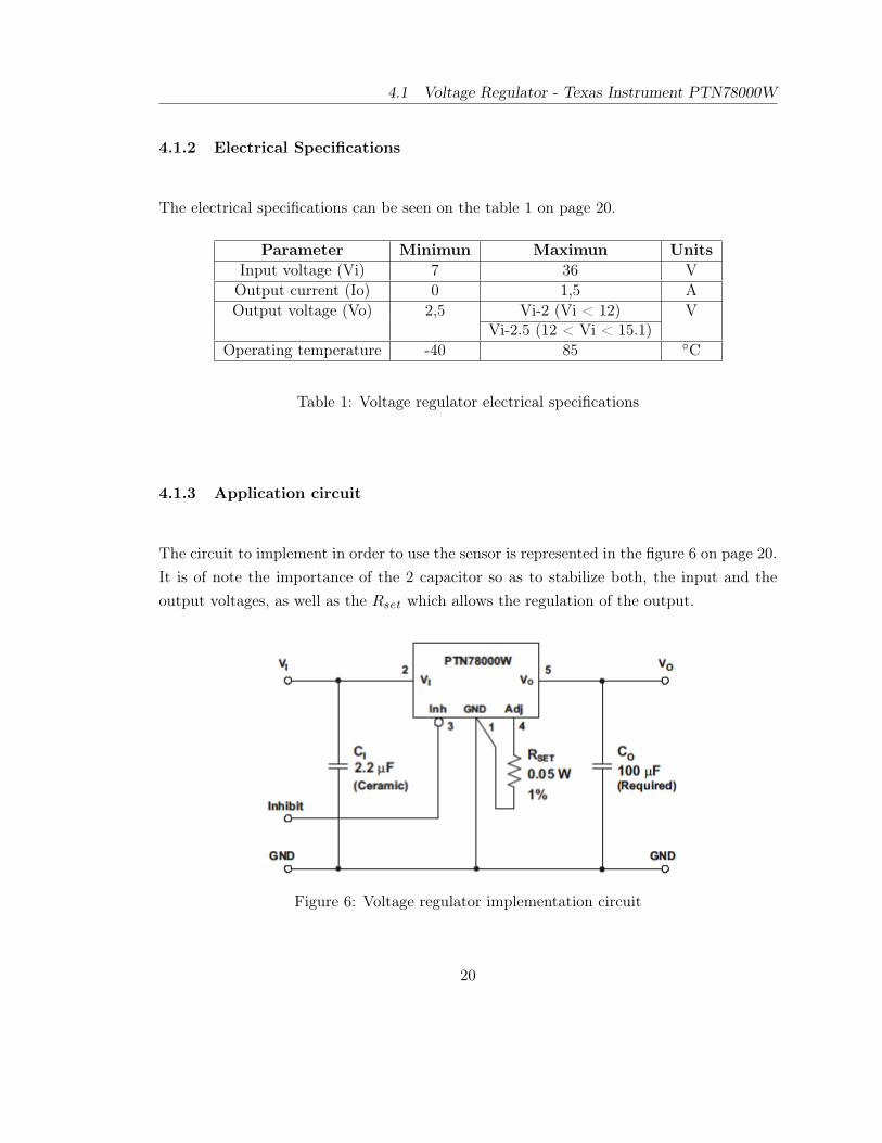
4.1.2 Electrical Specifications
The electrical specifications can be seen on the table 1 on page 20.
Parameter Minimun Maximun UnitsInput voltage (Vi) 7 36 VOutput current (Io) 0 1,5 AOutput voltage (Vo) 2,5 Vi-2 (Vi < 12) V
Vi-2.5 (12 < Vi < 15.1)Operating temperature -40 85 C
Table 1: Voltage regulator electrical specifications
4.1.3 Application circuit
The circuit to implement in order to use the sensor is represented in the figure 6 on page 20.It is of note the importance of the 2 capacitor so as to stabilize both, the input and theoutput voltages, as well as the Rset which allows the regulation of the output.
Figure 6: Voltage regulator implementation circuit
20

4 HARDWARE
4.1.4 Specific use in the project
Since the power supply to the car electronics comes from the slot track, and the nominalvoltage of this track is approximately 14 V, a voltage regulator is required in order toprovide a suitable voltage to every single electronic device.
In order to regulate the voltage, the resistor chosen was a potentiometer, so as to reach afinely-tuned output voltage . Considering that, the output of the regulator was set to 5 V,so that it can power all the electronic devices.
However, there is one exception, and it is the Baby Orangutan controller, which was powereddirectly from the track using a middle diode to reduce the voltage from 14 V to 13.3 V,since it can be powered up to 13.5 V. That fact lead to a faster speed in the slot car, sincethe higher the voltage of this controller the higher the power that the motor of the slot carmay obtain from the controller.
Moreover, in order to choose the capacitors in the input and output of this regulator, weconsidered the lose powers that the car suffer due to the non-continue power of the track,and therefore, we implemented two big capacitor of 1200 ηF, so that even when the carsuffers lose powers, the time that the car is off is minimum.
4.1.5 Power supply connection schematic
The figure 7 on page 22 illustrates the power supply schematic of our project. As it can beseen, V++ would be the power supply of the Orangutan controller, which is directly obtainedfrom the track using the diode D1, which not only reduces slightly the input voltage so thatit is suitable for the Orangutan, but also it protects the power supply against invertedconnections. On the other hand, Vin would be the 5 V regulated voltage for the otherdevices.
21

4.2 Baby Orangutan B-328 controller
Figure 7: Regulator and power supply connection circuit
4.2 Baby Orangutan B-328 controller
4.2.1 General description
The Baby Orangutan B-328 robot controllers is a complete control solutions for small robots.The small module includes a powerful Atmel ATmega 328P microcontroller, a TB6612FNGdual H-bridge for direct control of two DC motors, a 10k user potentiometer (connected toADC7), 18 user I/O lines 1 that can be used to expand the system, a green power LED, ared user LED (connected to PD1), a 20 MHz resonator, and a reverse-battery-protectionMOSFET. So a battery, motors, and sensors can be connected directly to the module tocreate simple robots.
4.2.2 Module pinout and component identification
The figure 8 on page 23 shows the Baby Orangutan module pinout and component identi-fication.
116 of which can be used as general-purpose digital I/Os and 8 of which can be used as analog inputchannels
22

4 HARDWARE
Figure 8: Baby Orangutan module pinout and component identification
• VIN is the input for the power supply
• RESET can be brought low to reset the controller, but it can otherwise be left dis-connected 1. This pin is labeled as PC6 in the ATmega48/168/328 datasheet (andon the Baby Orangutan silkscreen).
• Vcc can be used to tap into the Baby Orangutan’s regulated 5V line. This line cansupply a total of around 100 mA at 5 V, but thermal dissipation limits the total Vcccurrent to around 50 mA at 13.5 V.
• M1A and M1B are the outputs used to drive motor 1. These outputs can supplyaround 1 A continuous (3 peak).
• M2A and M2B are the outputs used to drive motor 2. These outputs can supplyaround 1 A continuous (3 peak).
• PC0 Ð PC5 can be used as both analog inputs and digital I/O lines.
• ADC6 and ADC7 are dedicated analog inputs. Note that ADC7 is internally con-nected to the 10k user trimmer potentiometer.
1It is internally pulled high
23

4.2 Baby Orangutan B-328 controller
• PB0, PB3, PB4, PB5, PD0, PD1, PD2, PD3, PD4, and PD7 are digital I/O lineswith alternate functions determined by the AVR ATmega 328P.
The table 2 on page 25 shows the alternate functions the differentes I/O ports can have.
4.2.3 Schematic
The figure 9 on page 24 shows the Baby Orangutan schematic.
Figure 9: Baby Orangutan schematic diagram
24

4 HARDWARE
Pin Orangutan Function Notes/Alternate Functions
PB0 digital I/O Timer1 input capture (ICP1) divided system clock output(CLK0)
PB1 digital I/O Timer1 PWM output A (OC1A)PB2 digital I/O Timer1 PWM output B (OC1B)PB3 M2 control line Timer2 PWM output A (OC2A) ISP programming linePB4 digital I/O Caution: also an ISP programming linePB5 digital I/O Caution: also an ISP programming linePB6 20 MHz resonator input not accessable to the userPB7 20 MHz resonator input not accessable to the userPC0 analog input and digital I/O ADC input channel 0 (ADC0)PC1 analog input and digital I/O ADC input channel 1 (ADC1)PC2 analog input and digital I/O ADC input channel 2 (ADC2)PC3 analog input and digital I/O ADC input channel 3 (ADC3)
PC4 analog input and digital I/O ADC input channel 4 (ADC4) I2C/TWI input/output dataline (SDA)
PC5 analog input and digital I/O ADC input channel 5 (ADC5) I2C/TWI clock line (SCL)
PC6 RESET pin Internally pulled high; active low digital I/O disabled bydefault
PD0 digital I/O USART input pin (RXD)
PD1 digital I/O Connected to red user LED (high turns LED on) USARToutput pin (TXD)
PD2 digital I/O External interrupt 0 (INT0)PD3 M2 control line Timer2 PWM output B (OC2B)
PD4 digital I/O USART external clock input/output (XCK) Timer0 externalcounter (T0)
PD5 M1 control line Timer0 PWM output B (OC0B)PD6 M1 control line Timer0 PWM output A (OC0A)PD7 digital I/OADC6 dedicated analog input ADC input channel 6 (ADC6)
ADC7 dedicated analog input Connected to user trimmer potentiometer ADC input chan-nel 7 (ADC7)
Table 2: Orangutan I/O pins description
25

4.2 Baby Orangutan B-328 controller
4.2.4 General specifications
The table 3 on page 26 shows the Baby Orangutan specifications.
Processor: ATmega328P @ 20 MHzRAM size: 2048 bytes
Program memory size: 32 KbytesMotor driver: TB6612FNG
Motor channels: 2User I/O lines: 182
Max current on a single I/O: 40 mAMinimum operating voltage: 5 VMaximum operating voltage: 13.5 V
Continuous output current per channel: 1 APeak output current per channel: 3 A
Maximum PWM frequency: 80 kHzReverse voltage protection?: Yes
Table 3: Orangutan general specifications
4.2.5 ATmega 328P microcontroller
The ATmega328P is a low-power CMOS 8-bit microcontroller based on the AVR enhancedRISC architecture. By executing powerful instructions in a single clock cycle, the AT-mega328P achieves throughputs approaching 1 MIPS per MHz allowing the system designerto optimize power consumption versus processing speed. The following microcontroller’sfeatures were used in our project:
1. Serial channel using USART protocol in the asynchronous operation mode. The serialchannel communicates the Wixel microcontroller in the car and the ATmega, so thedata can be sent to a computer, first from the ATmega to the Wixel through theserial channel, then through radiofrecuency from the Wixel to the other Wixel, andfinally from the Wixel connected to the computer to the computer through USB. Theserial channel is handled using its own interruption. The serial channel configuration:
• Baudrate: 115200 bps.
26

4 HARDWARE
• Parity bit
• 1 bits Stop
The µ uses 2 buffer to synchronize the sending/receiving with data writing/reading.The serial channel uses the port PD0 and PD1 as the channels to transmit and receivedata.
2. Serial channel with TWI(I2C) Master-Slave protocol. Being the µcontroller the Mas-ter, and the accelerometer, gyroscope and magnetometer in the IMU the three Slaveswhich will send data under the µcontroller request.
3. Timer 2 as PWM generator to control the motor driver which the Orangutan usesto power the motor of the car. PD3 and PB3 are the ports that the timer 2 usesas PWM generator. The timer 2 generates the PWM with a frequency of 9.8 kHzfrequency.
4. Analog-digital converter to read the analogs values of the Sharp sensor of distance.The ADC uses a 8-bit resolution with 13 µs conversion time, within a 0 and 5 Vrange, and a ±2 LSB accuracy. The ADC works in the single conversion mode, wherethe conversion ended is handled using the ADC interruption. The analog lectures isdone in the ADC6 channel.
5. Timer 0 with a interruption period to manage the power of the infrared LED thatmanages the switch. Inside the same interruption, the value of the Hall sensor ischecked. The Hall sensors builds the encoder, and since the encoder tick frequencyis always fewer than the infrared LED frequency, the interruption of the Timer 0can check the Hall sensor and detect the encoder edges. Moreover, inside the sameinterruption, and considering the period of the Timer 0, a time base is built in orderto manage other process which required precise execution, such as the PID, the cal-culation of the time between two tag readings or the time between different reports tosend to the computer. The programming of time base will be explained in the section7.1.7 in the page 86.
6. Ports PC0, PC1, PC2, PC3, PB1 and PB2 to read the 6 QTR-1RC sensors integratedin the QTR-8RC sensor. The lecture of those sensor is made every 200 µs, theminimum time required to charge the sensor capacitors, and let them discharge only
27

4.2 Baby Orangutan B-328 controller
with white surfaces, so that the difference between black and white lines can bedistinguish.
7. Timer 1 in normal mode, handled by interruption, to execute the QTR-8RC sensorevery 200 µs.
8. EEPROM memory to storage important system values such as the car speed or thecar mode of competition. That allows a easy system state recover after the car isreinitialized due to lose powers. This requirement is imposed since the car acquiresthe initial state after being programmed after being reinitialized, state that normallydiffers from the state that the car might have when a lose power occurs.
4.2.6 TB6612FNG dual H-bridge
This driver can supply the power to 2 different motors using 4 different outputs (M1A andM1B for the first motor, and M2A and M2B for the second one) . Our motor is controlledby M2A and M2B, which are controlled for PD3 and PB3 as inputs. As M2B is connectedto the positive pole on the motor, and M2A to the negative one, the table 4 on page 28explains how PD3 and PB3 manage the M2A and M2B, and how this management affectsthe motor’s power supply.
PD3 PB3 M2A M2B Motor effectH H L L BrakeL H L H ForwardH L H L ReverseL L Off (High imp.) Off (High imp.) Coast
Table 4: Motor Driver Truth Table (H = high, L = low)
As it can be seen, adjusting PB3 to a high level, and producing the PWM through PD3,the car would work switching between the forward mode and the brake mode. Since cyclingbetween drive and brake at high frequency results in variable motor speed that changesas a function of PWM duty cycle, if the pulse width of the PWM is increased(decreased),the car would acquired less(more) power supply, and due to that it would have less(more)speed.
28

4 HARDWARE
4.2.7 Specific use in this project
As the main piece of the hardware, the main function of this controller is acquire datafrom every sensor, either using the Serial Channel with the TWI protocol to establish thecommunication with the IMU, the conversion of the A/D converter for the Sharp sensorvalues or checking the digital ports for the QTR or the Hall sensor values. With those tools,it makes periodical readings of every sensor, sending this data afterwards to the computerwith a programable period.
Moreover, this controller establishes a time base to control with precision different resourcesin our system, as well as it regulates the car speed using a PID which takes the encoderas input, and outputs the required PWM duty cycle. Is is also of note, that the EEPROMmemory of the µcontroller is used to storage the values of the system, so that when a losepower occurs and the car is reinitialized, it can easily recover its previous state without anycommunication with the computer. That is required because when there is a lose power, thecar recovers the initial state that it had right after being programmed, state that normallydiffers from the car state in the middle of a race in settings like the car speed or the carmode of competition.
Furthermore, it uses the Serial Channel with USART protocol to communicate with theWixel microcontroller, which receives data from the Orangutan and sends it to the computerthrough Radio communication. In addition, it also controls the power supply to the carmotor through its TB6612FNG dual H-bridge, which results in the possibility of car speedregulation.
Finally, it is also responsible for the activation of the infrared led that allows the track-sideswitching as well as the communication and control of the small hardware connected to theport track, which manages the switches on the Switch piece.
4.3 QTR-8RC Reflectance Sensor Array
4.3.1 General description
The Pololu QTR-8RC reflectance sensor array are intended as line sensors, but they canbe used as a general-purpose proximity or reflectance sensors. Each module is a convenient
29

4.3 QTR-8RC Reflectance Sensor Array
carrier for eight infrared pairs of emitter and receiver phototransistor1 evenly spaced atintervals of 9.525mm. The outputs are all independent, but the LEDs are arranged in pairsto halve current consumption.
Each QTR-1RC reflectance sensor phototransistor output is tied to a capacitor dischargecircuit, as is shown on the figure 10 on page 30, so that if the capacitor is charged and theLED is turned on, the discharge time of the capacitor depends on how reflecting is whateverthe sensor is reading2, which allows a digital I/O line on a microcontroller to take an analogreflectance reading by measuring the discharge time of the capacitor.
Figure 10: QTR-1RC sensor schematic
When you have a microcontroller’s digital I/O connected to a sensor output, the typicalsequence for reading that sensor is:
1. Set the I/O line to an output and drive it high.
2. Allow at least 10us for the 10nF capacitor to charge.
3. Make the I/O line an input (high impedance).
4. Measure the time for the capacitor to discharge by waiting for the I/O line to go low.
1Each one of this pairs is the sensor QTR-1RC from Pololu2the shorter the time, the more reflective the surface
30
4 HARDWARE
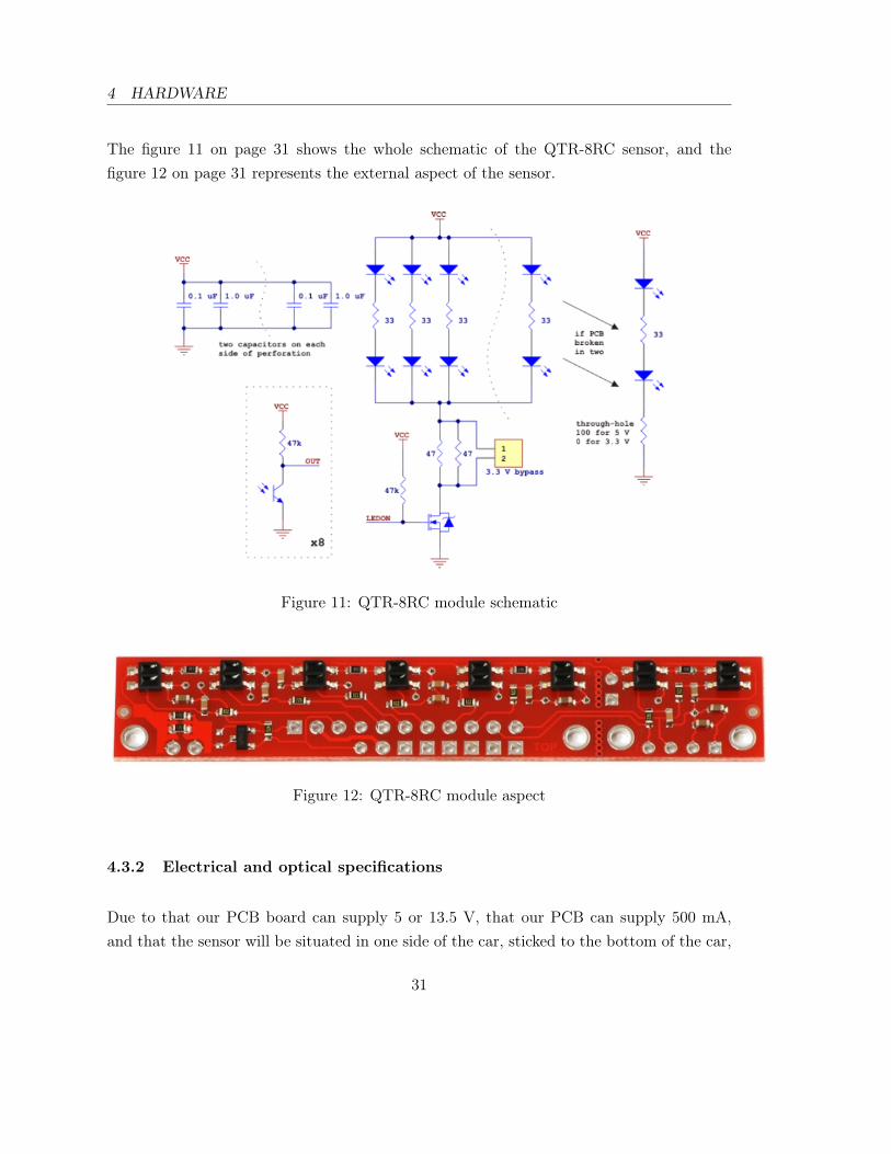
The figure 11 on page 31 shows the whole schematic of the QTR-8RC sensor, and thefigure 12 on page 31 represents the external aspect of the sensor.
Figure 11: QTR-8RC module schematic
Figure 12: QTR-8RC module aspect
4.3.2 Electrical and optical specifications
Due to that our PCB board can supply 5 or 13.5 V, that our PCB can supply 500 mA,and that the sensor will be situated in one side of the car, sticked to the bottom of the car,
31
4.3 QTR-8RC Reflectance Sensor Array
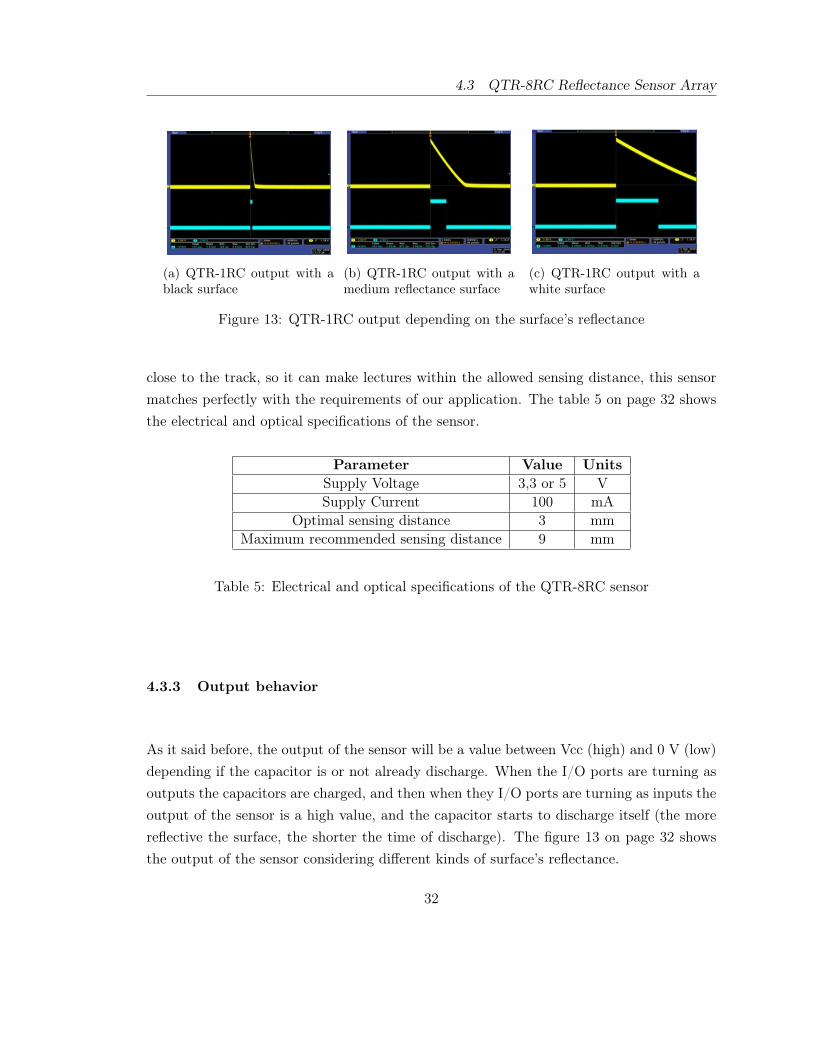
(a) QTR-1RC output with ablack surface
(b) QTR-1RC output with amedium reflectance surface
(c) QTR-1RC output with awhite surface
Figure 13: QTR-1RC output depending on the surface’s reflectance
close to the track, so it can make lectures within the allowed sensing distance, this sensormatches perfectly with the requirements of our application. The table 5 on page 32 showsthe electrical and optical specifications of the sensor.
Parameter Value UnitsSupply Voltage 3,3 or 5 VSupply Current 100 mA
Optimal sensing distance 3 mmMaximum recommended sensing distance 9 mm
Table 5: Electrical and optical specifications of the QTR-8RC sensor
4.3.3 Output behavior
As it said before, the output of the sensor will be a value between Vcc (high) and 0 V (low)depending if the capacitor is or not already discharge. When the I/O ports are turning asoutputs the capacitors are charged, and then when they I/O ports are turning as inputs theoutput of the sensor is a high value, and the capacitor starts to discharge itself (the morereflective the surface, the shorter the time of discharge). The figure 13 on page 32 showsthe output of the sensor considering different kinds of surface’s reflectance.
32

4 HARDWARE
4.3.4 Breaking the sensor in 2 modules
One of the properties of this sensor is that the use of the 8 sensors is not mandatory. Inother word, the sensor can be separated in 2 modules, one with 6 QTR-1RC sensors, andthe other one with just 2 QTR-1RC sensors. As a result, our project uses just the modulewith 6 sensors, because it’s more than enough for our application, and also because the 8sensor module doesn’t fit in the side of the car due to its huge dimensions.
The board can be easily separated using a knife or a box cutter. If the board is separated,and the module with 2 sensors is supposed to be used, a 100 Ohm resistor must be includedin the board. The figure 14 on page 33 shows the sensor when it’s separated.
Figure 14: QTR-8RC board separated
4.3.5 Specific use in the project
The sensor task is reading different codes the circuit track will have so as to distinguish thedifferent sort of pieces. Since the sensor can easily distinguish a white and a black colorthrough the discharge time of the capacitor, the track will have different codes along thecircuit, codes that using a black-white combination of 6 values will identify the sort of piece.Nevertheless, since 2 of the 6 code values are used as codes detector 1, there are actually24 values that the codes can use. The description of those codes can be found on the thetable 14 on page 69.
1The first and last value codes are always white, so that when the last sensor and the first one read awhite means that the sensor is detecting a new code
33

4.3 QTR-8RC Reflectance Sensor Array
In order to make the readings, the microcontroller charges the capacitors (turning the I/Oports into outputs), and then wait a time T, after this time T the microcontroller checksthe value of each QTR-1RC sensor. If the output of the sensor is low, it means that thecapacitor of this sensor has been discharged, and thus, this sensor is reading a white. Onthe other hand, a high level means that the capacitor didn’t suffer a completely discharging,so that the sensor must be reading a black. The time T was selected considering the timethreshold for the discharging of the capacitor in our application when the sensor is readinga white, and its value is around 200 µs.
4.3.6 Connection schematic
The figure 15 on page 34 illustrates the connections between the QTR and the Orangutanmicrocontroller, which uses 6 of its 6 I/O ports to read the value of the QTR sensor. It canalso be seen that the QTR is powered with Vin, and the microcontroller with V++, valuesthat can be observed on the schematic of the voltage regulator (Figure 7, page 22).
(a) Orangutan B-328 controller
(b) QTR
Figure 15: Orangutan - QTR connections
34

4 HARDWARE
4.4 Distance measuring optoelectronic sensor Sharp GP2D120
4.4.1 General description
The GP2D120 is a distance measuring sensor with integrated signal processing and analogvoltage. It uses a LED as a light emitter, and it uses a photoreceptor to know if the lightemitted by the LED is reflecting somewhere, in that case considering the intensity of thereflexion it can give a value of the object distance that has provoke the reflection.
Since the intensity of the reflexion is not an electrical value, the sensor uses a processingcircuit to transform that measurement into an electrical one, because of that, the outputof the sensor is an analog signal. The effective range of measurement of the sensor is from4 cm to 30 cm. The figure 16 on page 35 shows the schematic of the sensor.
Figure 16: Sharp sensor schematic
4.4.2 Electrical and electrooptical Specifications
Due to that our PCB board can supply 5 or 13.5 V, that our PCB can supply 500 mA,and that the sensor must detect if there is another car in front of it and get the distancebetween the other car and itself, so a 4-30 cm. range of measuring distance is perfect todo that task, this Sharp sensor matches perfectly with the requirements of our application.The table 6 on page 36 shows the electrical and electrooptical specifications of the sensor.
35

4.4 Distance measuring optoelectronic sensor Sharp GP2D120
Parameter Minimun Typical Maximun UnitsOperating supply voltage (Vcc) 4,5 — 4,5 V
Operating temperature -10 — 60 CMeasuring distance Range 4 — 30 cm
Average supply current (L=30 cm) 33 50 mA
Table 6: Sharp sensor electrical and optoelectronic specifications, where L = distance toreflective object
4.4.3 Output behavior
The output of the sensor is an analog signal whom value can be between 0.25 and 3.1 Vdepending on the measuring distance. When the distance is 30 cm the sensor gets theminimum value, and when it is 4 cm the maximum one. So, to measure the analog outputthe output of the sensor has been connected to one of the channels of the analog-digitalconverter on the ATmega328P microcontroller.
The table 7 on page 36 shows the range value of the sensor output according to the distanceto the reflective object, and the figure 17 on page 37 shows the typical value of the outputaccording to the distance to the reflective object.
Parameter Conditions Minimun Typical Maximun UnitsOutput terminal voltage (Vo) L=30 cm 0,25 0,4 0,55 V
Output voltage difference
Change in theoutput when Lchanges from 30cm to 4 cm
1,95 2,25 2,55 V
Table 7: Sharp sensor output value, where L = distance to reflective objetc
4.4.4 Specific use in the project
The sensor task on our project is the detection of another slot-car in front of it and theacquisition of the distance between the other car and itself. Detecting another car allowsthe car to take decisions as break to avoid a crash or to activate a switch track change and
36

4 HARDWARE
Figure 17: Sharp sensor output graphic. ab
aThe continuos line represents the output with white paper (90% Reflectance) as the reflective objectand the dash one represents grey paper (18% Reflectance)
bSupply Voltage of 5 V and an environmental temperature of 25 C has been used to get the Output-Distance relation
37

4.4 Distance measuring optoelectronic sensor Sharp GP2D120
try to overtake the other car.
The problem with this sensor is that with distances lesser than 4 cm, the output invertsthe values of the sensor, so that, for instance, an object that is 2 cm away from the sensorwould provoke a sensor output value of 2.2 V, the same output that an object 5.5 cm awaywould provoke. In order to avoid this problem, the car’s control algorithm has a functionthat doesn’t let the car go further than 4 cm from a car in front of it, making the car breakbefore the 4 cm threshold is reached, and being able to know when a track change mightbe suitable so as to overtake the other car using a different track side.
4.4.5 Connection schematic
The figure 18 on page 38 illustrates the connections between the Sharp sensor and theOrangutan microcontroller, which uses one of its A/D convertion-ports to read the analogvalue of analog Sharp sensor. It can also be seen that the Sharp is powered with Vin, andthe microcontroller with V++, values that can be observed on the schematic of the voltageregulator (Figure 7, page 22).
(a) Orangutan B-328 controller
(b) Sharp sensor
Figure 18: Orangutan - Sharp sensor connections
38

4 HARDWARE
4.5 Hall effect sensor - Melexis US1881
4.5.1 General description
Based on mixed signal CMOS technology, Melexis US1881 is a Hall-effect device with highmagnetic sensitivity. This multi-purpose latch suits most of the application requirements.
The chopper-stabilized amplifier uses switched capacitor technique to suppress the offsetgenerally observed with Hall sensors and amplifiers. The CMOS technology makes thisadvanced technique possible and contributes to smaller chip size and lower current con-sumption than bipolar technology. The small chip size is also an important factor tominimize the effect of physical stress. This combination results in more stable magneticcharacteristics and enables faster and more precise design.
The output signal is open-drain type. Such output allows simple connectivity with TTLor CMOS logic by using a pull-up resistor tied between a pull-up voltage and the deviceoutput. The figure 19 on page 39 shows the schematic of the sensor.
Figure 19: Hall sensor schematic
39

4.5 Hall effect sensor - Melexis US1881
4.5.2 Electrical and Magnetical Specifications
Due to that our PCB board can supply 5 or 13.5 V, that the rotation frequency of thewheel is smaller than the maximum switching frequency of the sensor, that buying magnetswith a magnet field smaller than 9.5 mT is easy, and that our PCB can supply 500 mA,this Hall sensor matches perfectly with our application. The table 8 on page 40 shows theelectrical and magnetical specifications of the sensor.
Parameter Minimun Maximun UnitsSupply Voltage (Vdd) 3,5 24 V
Supply Current 5 mAMaximum Switching Frequency 10 Khz
Operating point (Bop) 0,5 9,5 mTRelease Point (Brp) -9,5 -0,5 mT
Hysteresis 7 12 mT
Table 8: Hall sensor electrical and magnetic specifications
4.5.3 Output Behaviour versus Magnetic Pole
Because of the High level of the sensor, which is always the value of the supply voltage, thesupply voltage of the sensor was 5 V since that voltage level can be read directly by theI/O ports of the ATmega328P microcontroller. The table 9 on page 40 and the figure 20on page 41 shows the output of the sensor considering the value of the magnetic field.
Parameter Condition Out UnitsSouth pole B < Brp Vdd VNorth pole B > Bop 0 V
Table 9: Hall Sensor Output
4.5.4 Application circuit
According to the data sheet of the Hall sensor, the circuit to implement in order to use thesensor is represented in the figure 21 on page 41.
40

4 HARDWARE
Figure 20: Hall sensor output
Figure 21: Hall sensor implementation circuit
41

4.5 Hall effect sensor - Melexis US1881
4.5.5 Specific use in the project
Since the Hall sensor behaves as a latch with symmetric operating and release switchingpoints (BOP=|BRP|), magnetic fields with equivalent strength and opposite direction drivethe output high and low. On contrast, removing the magnetic field (B = 0) without anopposite field keeps the output in its previous state.
Due to those 2 facts, we can use the Hall sensor as an encoder. In order to do that, aseries of 20 north-south poles alternated magnets were sticked to the wheel of the car, andthe Hall sensor was fixed in the same position, detecting the transition of those magnets.Thanks to the specifications of the Hall sensor, each transition of a magnet will provoquea change in the output of the Hall sensor, so the output will be a serial pulse, where thefrecuency of this pulse would be 20 time as many as the rotation frequency of the wheel.
Considering that the diameter of the car wheel is approximately 23 mm, the angular speedof the wheel and the linear speed of the car can be easily calculated, and the equation 2 inthe page 42 shows the completely algorithm.
AngularSpeed =encoderPulses
20× 2π × 1
δtReadings
(rads
)Linear Speed = Angular Speed ×0.023
2
(ms
) (2)
4.5.6 Connection schematic
The figure 22 on page 43 illustrates the connections between the Hall sensor and theOrangutan microcontroller, which uses a digital port of in order to count the number ofpulses that the Hall sensor produces. It can also be seen that the Sharp is powered withVin, and the microcontroller with V++, values that can be observed on the schematic of thevoltage regulator (Figure 7, page 22).
42

4 HARDWARE
(a) Orangutan B-328 controller
(b) Hall sensor
Figure 22: Orangutan - Hall sensor connections
4.6 IMU - MinIMU-9 v2
4.6.1 General description
The MinIMU-9 v2 is an inertial measurement unit (IMU) that has integrated a L3GD203-axis gyro and a LSM303DLHC 3-axis accelerometer and 3-axis magnetometer. Incorpo-rating a I2C/TWI interface, it allows a quick access to the nine independent measurements,providing thus, the calculation of the sensor orientation and position.
In addition, it also has packed a linear voltage regulator that supplies the 3.3 V requiredto power the devices previously mentioned through 2.5-5.5 V electric sources, making easythe connection with microcontrollers operating at 5 V. Moreover, this 3.3 V can accessedtrough a terminal, allowing the power of extra devices. All this features are integrated ontoa tiny 20 x 13 mm board, the figure 23 on page 44 illustrates the board and its dimensions:
On the other hand, the schematic of the sensor can be observed on the figure 24 on page 45.
43

4.6 IMU - MinIMU-9 v2
Figure 23: IMU general illustration and dimensions
4.6.2 Technical Specifications and Pin Description
The table 10 on page 44 illustrates the electrical and technical specifications of the sensor,and the table 11 on page 46 shows the pin description.
Parameter Minimun Typical Maximun UnitsSupply Voltage (VIN) 2,5 5,5 V
Supply Current 10 mAGyro measurement range ±250 ±2000 ą/s
Accelerometer measurement range ±2 ±16 gMagnetometer measurement range ±1, 3 ±8, 1 gauss
Regulator Output (VDD) 5 VRegulator Current 150 mA
Dimensions 20 x 13 x 3 mm
Table 10: IMU technical specifications
4.6.3 TWI protocol
The TWI bus is a multiMaster serial bus with the same specifications than the commercialversion I2C from Phillips. Therefore, through the description of this project, any referenceto I2C will be in fact to TWI, since the only difference is that I2C is the name for thecommercial version. This bus isused in fast speed communications between at least oneMaster and one Slave, and it uses two bidirectional open-drain lines, Serial Data Line (SDA)
44

4 HARDWARE
Figure 24: IMU schematic
45

4.6 IMU - MinIMU-9 v2
PIN DescriptionSCL Level-shifted I2C clock line: HIGH is VIN, LOW is 0 VSDA Level-shifted I2C data line: HIGH is VIN, LOW is 0 VGND The ground (0 V) connection for the power supply.
VIN This is the main 2.5 - 5.5 V power supply connection. The SCL andSDA level shifters pull the II2C bus high bits up to this level.
VDD
3.3 V regulator output or low-voltage logic power supply, depending onVIN. When VIN is supplied and greater than 3.3 V, VDD is a regulated3.3 V output that can supply up to approximately 150 mA to externalcomponents. Alternatively, when interfacing with a 2.5 - 3.3 V system,VIN can be left disconnected and power can be supplied directly to VDD.
Table 11: IMU Pin description
and Serial Clock (SCL), with pull-up resistors. Moreover, it posses 3 several different regularclock frequencies, however, in this project the Fast Speed Mode was used (400 KHz).
In our project, the µController is the Master, which establishes the communications withthe 3 Slaves: magnetometer, accelerometer and gyroscope. As a first step, the TWI must beconfigure, and in order to do that, the Orangutan must indicate to the Slaves the differentconfiguration parameters.
Since the IMU can acquire data either on demand1 or cyclic 2, the cyclic configuration hasbeen chosen so as to reach quicker readings of current available data. That is because, sincethe Slaves are reading regularly the data, they can provide all the time with the last sensormeasures, therefore, the µ Controller as a Master only has to send a request to get the lastdata readings, avoiding the previous request to the Slave for the acquisition of a new data.
Concerning the TWI operation, basically, every Master can ask requests to the differentSlaves, and the Slave can answer under specific petition to the specific Master. Moreover,every device has a register that specify the current status of the TWI bus, and because thestatus are predefined, this register can be checked in order to know if the communicationshas failed.
Looking the protocol in detail, the communications on the bus starts through a START
1Demand: the microcontroller have to send a request to the specific Slave asking for the data acquisition2Cyclic: the Slaves read data regularly without asking
46
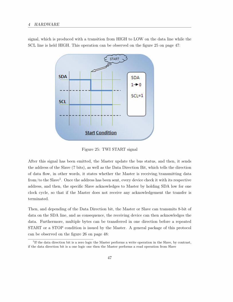
4 HARDWARE
signal, which is produced with a transition from HIGH to LOW on the data line while theSCL line is held HIGH. This operation can be observed on the figure 25 on page 47:
Figure 25: TWI START signal
After this signal has been emitted, the Master update the bus status, and then, it sendsthe address of the Slave (7 bits), as well as the Data Direction Bit, which tells the directionof data flow, in other words, it states whether the Master is receiving/transmitting datafrom/to the Slave1. Once the address has been sent, every device check it with its respectiveaddress, and then, the specific Slave acknowledges to Master by holding SDA low for oneclock cycle, so that if the Master does not receive any acknowledgement the transfer isterminated.
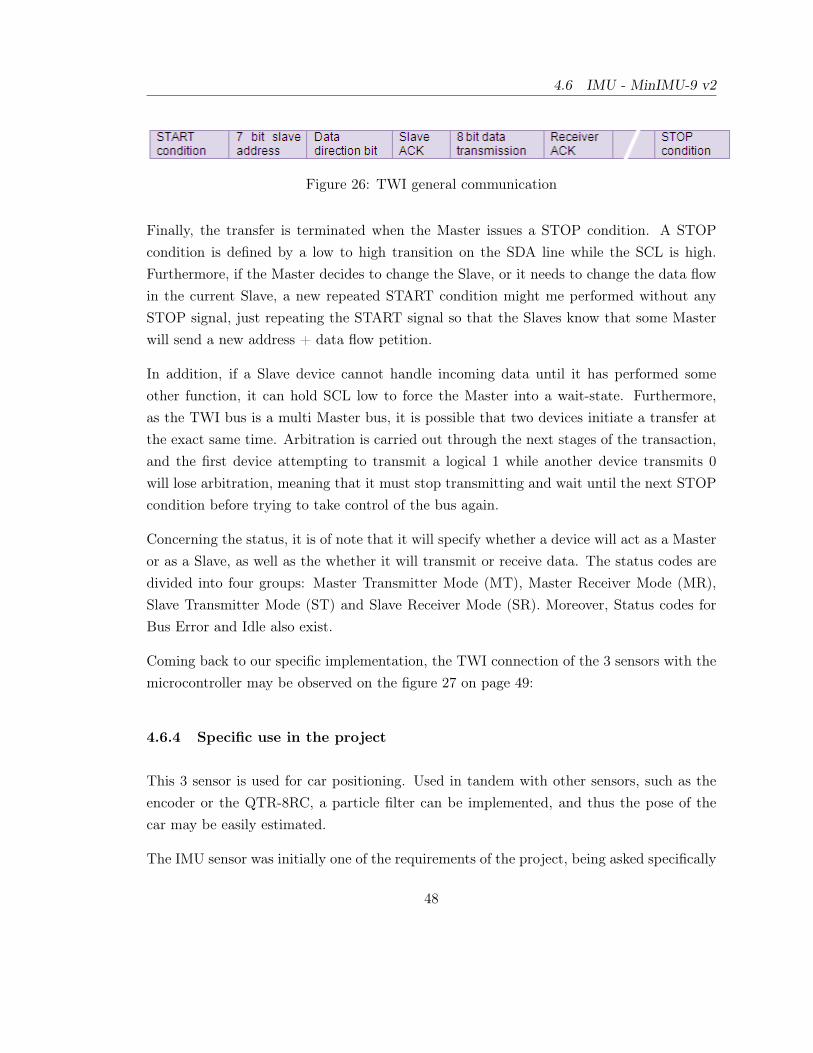
Then, and depending of the Data Direction bit, the Master or Slave can transmits 8-bit ofdata on the SDA line, and as consequence, the receiving device can then acknowledges thedata. Furthermore, multiple bytes can be transferred in one direction before a repeatedSTART or a STOP condition is issued by the Master. A general package of this protocolcan be observed on the figure 26 on page 48:
1If the data direction bit is a zero logic the Master performs a write operation in the Slave, by contrast,if the data direction bit is a one logic one then the Master performs a read operation from Slave
47
4.6 IMU - MinIMU-9 v2
Figure 26: TWI general communication
Finally, the transfer is terminated when the Master issues a STOP condition. A STOPcondition is defined by a low to high transition on the SDA line while the SCL is high.Furthermore, if the Master decides to change the Slave, or it needs to change the data flowin the current Slave, a new repeated START condition might me performed without anySTOP signal, just repeating the START signal so that the Slaves know that some Masterwill send a new address + data flow petition.
In addition, if a Slave device cannot handle incoming data until it has performed someother function, it can hold SCL low to force the Master into a wait-state. Furthermore,as the TWI bus is a multi Master bus, it is possible that two devices initiate a transfer atthe exact same time. Arbitration is carried out through the next stages of the transaction,and the first device attempting to transmit a logical 1 while another device transmits 0will lose arbitration, meaning that it must stop transmitting and wait until the next STOPcondition before trying to take control of the bus again.
Concerning the status, it is of note that it will specify whether a device will act as a Masteror as a Slave, as well as the whether it will transmit or receive data. The status codes aredivided into four groups: Master Transmitter Mode (MT), Master Receiver Mode (MR),Slave Transmitter Mode (ST) and Slave Receiver Mode (SR). Moreover, Status codes forBus Error and Idle also exist.
Coming back to our specific implementation, the TWI connection of the 3 sensors with themicrocontroller may be observed on the figure 27 on page 49:
4.6.4 Specific use in the project
This 3 sensor is used for car positioning. Used in tandem with other sensors, such as theencoder or the QTR-8RC, a particle filter can be implemented, and thus the pose of thecar may be easily estimated.
The IMU sensor was initially one of the requirements of the project, being asked specifically
48

4 HARDWARE
Figure 27: IMU TWI connection
for the tutor. Nevertheless, when it was tested on our specific project two difficulties werefounded.
The first one was that the slot track and the motor induced vibrations on the IMU, and asconsequence the noise in the accelerometer was around 5 times as many as the correct valueof the measures. Despite the fact that several techniques were tried, such as an low-passfilter or a mechanic isolation of the IMU, in order to reduce the noise, no one of them wassuccessful, and as a consequence the use of the accelerometers was not possible.
Likewise, a magnetic noise was induced on the magnetometer due to the encoder magnets,resulting similarly in a useless magnetometer, and leaving the gyroscope as the only sensoravailable on the IMU.
Nevertheless, the implementation of the particle filter was possible using the shape of the
49

4.6 IMU - MinIMU-9 v2
track as one part of the update step, taking the place of the magnetometer measures.Similarly, the problem with the accelerometer was solved combining the measures of theencoder and the tag track lectures. However, it is not the goal of this section look at thedetails of the filter, instead, this insight will be explained later on in this document.
4.6.5 Connection schematic
The figure 28 on page 50 illustrates the connections between the IMU sensor and theOrangutan microcontroller, which uses its I2C ports (PC4 as SDA and PC5 as SDL) inorder to read the data from the 3 Slaves sensors inside the IMU. It can also be seen that theIMU is powered with Vin, and the microcontroller with V++, values that can be observedon the schematic of the voltage regulator (Figure 7, page 22).
(a) Orangutan B-328 controller
(b) IMU sensor
Figure 28: Orangutan - IMU sensor connections
50

4 HARDWARE
4.7 Wixel Programmable USB Wireless Module
4.7.1 General description
The Wixel is a general-purpose programmable device based on the CC2511F32 microcon-troller from Texas Instruments, which has integrated a radio transceiver, 32 KB of flashmemory, 4 KB of RAM, a full-speed USB interface and a voltage regulator. A total of 15general-purpose I/O lines are available, including 6 analog inputs.
All that features allows a single Wixel to adapt the Serial Data transmission to USB andvice versa, as well as the Serial to Radio or USB to Radio thanks to its Radio transmitter.Likewise, featuring a 2.4 GHz radio and USB, the implementation of 2 Wixel it is a goodsolution to create a wireless connection between 2 devices. Obviously, the Wixel’s radio isnot compatible with Wi-Fi, Zigbee, or Bluetooth.
The figure 29 on page 51 illustrates the board and its dimensions:
Figure 29: Wixel general illustration and dimensions
4.7.2 Module pinout and component identification
The figure 30 on page 52 shows the Wixel module pinout and component identification.
51

4.7 Wixel Programmable USB Wireless Module
Figure 30: Wixel module pinout and component identification
• USB is the mini-USB port connection to connect the Wixel to a computer. The USBconnection is used to configure the Wixel, as well as to transmit and receive data.The USB connection can also provide power to the Wixel.
• RF antenna, located on the opposite side of the USB connection is the 2.4 GHz PCBtrace antenna. This antenna, along with the other RF circuitry, forms a radio thatallows the Wixel to send and receive data packets in the 2.4 GHz band.
• VIN is the input for the power supply.
• The three interlinked GND pins are at 0 V by definition.
• RESET can be brought low to reset the controller, but it can otherwise be left dis-connected1.
1It is internally pulled high
52

4 HARDWARE
• 3V3 is connected to the output of the Wixel’s 3.3 V regulator. This power source canbe used to power other low-current peripherals in your system.
• VALT pin is connected to three things: the 5V USB bus power from the USB port(through a diode), VIN (through a diode), and to the input of the WixelÕs on-board 3.3 V regulator. The connection to 5V is switched off when a power supply isconnected to VIN. It can be used as a power supply.
• P0_x / P1_x / P2_x are 15 I/O lines. They are supposed to work with 3.3 V,therefore level-shifters, diodes, or voltage dividers must be used so as to connect theWixel to outputs from 5V systems. Their behavior depends on the application thatis loaded into the Wixel:
1. USART0 and USART1 can perform asynchronous serial or SPI communication.
2. 3 timers that allow the creation of PWM output.
3. 6 analog input (A0 - A5) connected to a 7 - 12 bit analog-digital converter.
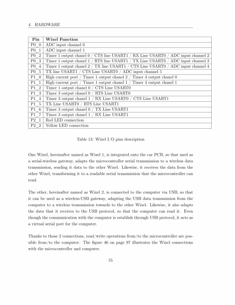
The table 12 on page 55 illustrates a more exhaustive insight of the alternative functionsthat the different I/O ports can have. It is of note that the both, the USART 0 and theUSART 1 Serial Port can be used through 2 different pin groups. Likewise, both the timer1 and timer 3 and can select their different channels through 2 different pins.
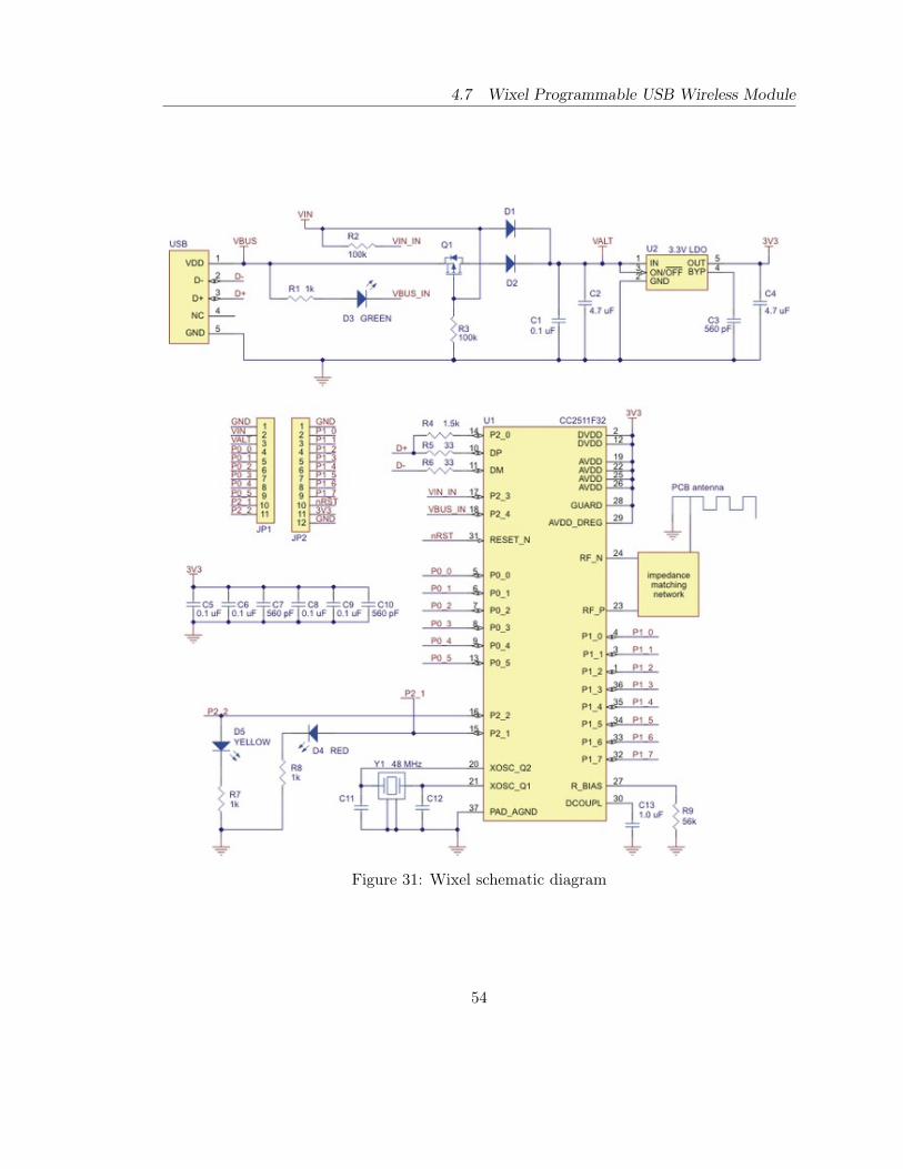
4.7.3 Schematic
The figure 31 on page 54 shows the Wixel schematic.
4.7.4 General specifications
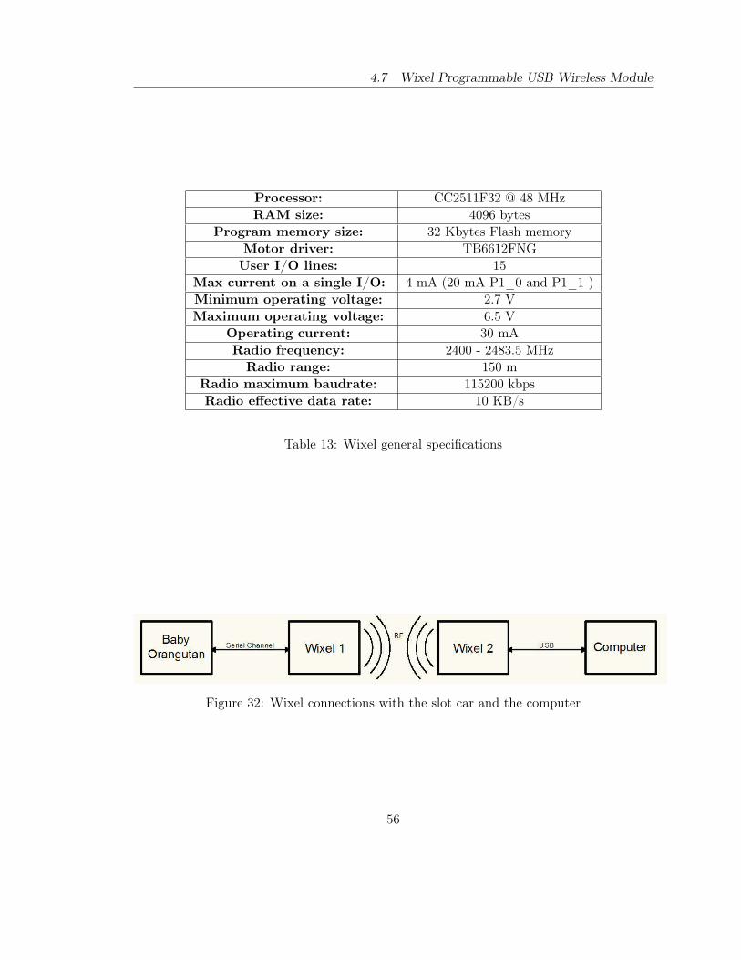
The table 13 on page 56 shows the Baby Orangutan specifications.
4.7.5 Specific use in the project
For this project 2 Wixels have been used, so that a connection between the computer andthe slot car is possible.
53
4.7 Wixel Programmable USB Wireless Module
Figure 31: Wixel schematic diagram
54
4 HARDWARE
Pin Wixel FunctionP0_0 ADC input channel 0P0_1 ADC input channel 1P0_2 Timer 1 output chanel 0 / CTS line USART1 / RX Line USART0 / ADC input channel 2P0_3 Timer 1 output chanel 1 / RTS line USART1 / TX Line USART0 / ADC input channel 3P0_4 Timer 1 output chanel 2 / TX line USART1 / CTS Line USART0 / ADC input channel 4P0_5 TX line USART1 / CTS Line USART0 / ADC input channel 5P1_0 High current port / Timer 1 output chanel 2 / Timer 4 output chanel 0P1_1 High current port / Timer 1 output chanel 1 / Timer 4 output chanel 1P1_2 Timer 1 output chanel 0 / CTS Line USART0P1_3 Timer 3 output chanel 0 / RTS Line USART0P1_4 Timer 3 output chanel 1 / RX Line USART0 / CTS Line USART1P1_5 TX Line USART0 / RTS Line USART1P1_6 Timer 3 output chanel 0 / TX Line USART1P1_7 Timer 3 output chanel 1 / RX Line USART1P2_1 Red LED connectionP2_2 Yellow LED connection
Table 12: Wixel I/O pins description
One Wixel, hereinafter named as Wixel 1, is integrated onto the car PCB, so that used asa serial-wireless gateway, adapts the microcontroller serial transmission to a wireless datatransmission, sending it data to the other Wixel. Likewise, it receives the data from theother Wixel, transforming it to a readable serial transmission that the microcontroller canread.
The other, hereinafter named as Wixel 2, is connected to the computer via USB, so thatit can be used as a wireless-USB gateway, adapting the USB data transmission from thecomputer to a wireless transmission towards to the other Wixel. Likewise, it also adaptsthe data that it receives to the USB protocol, so that the computer can read it. Eventhough the communication with the computer is establish through USB protocol, it acts asa virtual serial port for the computer.
Thanks to those 2 connections, read/write operations from/to the microcontroller are pos-sible from/to the computer. The figure 46 on page 97 illustrates the Wixel connectionswith the microcontroller and computer.
55
4.7 Wixel Programmable USB Wireless Module
Processor: CC2511F32 @ 48 MHzRAM size: 4096 bytes
Program memory size: 32 Kbytes Flash memoryMotor driver: TB6612FNGUser I/O lines: 15
Max current on a single I/O: 4 mA (20 mA P1_0 and P1_1 )Minimum operating voltage: 2.7 VMaximum operating voltage: 6.5 V
Operating current: 30 mARadio frequency: 2400 - 2483.5 MHzRadio range: 150 m
Radio maximum baudrate: 115200 kbpsRadio effective data rate: 10 KB/s
Table 13: Wixel general specifications
Figure 32: Wixel connections with the slot car and the computer
56

4 HARDWARE
4.7.6 Connection schematic
The figure 33 on page 57 illustrates the connections between the Wixel microcontroller onthe car, and the Orangutan microcontroller, which uses its USART ports 1 in order toestablish a serial communication between the 2 microcontrollers. It is of note the use of the3 resistors on the Orangutan transmission line, which used as a voltage divider, they adaptthe 5 output voltage of the Orangutan to the 3.3 input voltage of the Wixel. It can also beseen that the IMU is powered with Vin, and the microcontroller with V++, values that canbe observed on the schematic of the voltage regulator (Figure 7, page 22).
(a) Orangutan B-328 controller (b) Wixel microcontroller
Figure 33: Orangutan - Wixel connections
4.8 Printed circuit board (PCB)
4.8.1 General description
In order to mount and pack all the hardware, a PCB was designed using the software KiCad,and then it was ordered its production to an external enterprise. The PCB integrates andpacks all the hardware onto a 3.7 x 11.4 cm board.
1PD0 as RxD and PD1 as TXD
57

4.9 Board for switch management
The figure 34 on page 59, and the figure 35 on page 60, show the front and back side of thePCB, with a detailed description of the hardware location.
4.8.2 Secondary PCB
A secondary smaller PCB connected to the the main one was also designed. Its only functionis packing the circuit associated with the small infrared led in the bottom of the car, whichactivates the track switches on the slot track, allowing the car to change the track side.The figure 36 on page 61, show the front and back side of the PCB.
The figure 37 on page 61 illustrates the connections between the infrared Led on the sec-ondary PCB, and the Orangutan microcontroller. It is quite clear that CONN_2 representsthe connection between both PCB, so that the microcontroller can power through its PB0the circuit in the secondary board.
4.9 Board for switch management
4.9.1 General description
One of the specific pieces where the slot car might race is a switch piece where the car canchoose whether it wants to swap the track side or not. A image of this kind of track canbe seen on the figure 41d on page 68.
In order to do this side switch, not only the small led previously mentioned (section 36)is needed, but also a small hardware circuit, which communicates the computer with oneof the ports where the regular manual controllers are connected, is required. Basically, themain function of this circuit is transform the orders through USB from the computer, intoan signal order to this port.
4.9.2 Hardware required
So as to build this circuit, different hardware is needed. The goal of this section will bedescribe it.
58

4 HARDWARE
Figure 34: PCB front side
59

4.9 Board for switch management
Figure 35: PCB back side
60

4 HARDWARE
Figure 36: Secondary board
(a) Orangutan B-328 controller (b) Infrared Led
Figure 37: Orangutan - Infrared Led connections
61

4.9 Board for switch management
1. USB port: it is the entry of the data from the computer, and it allows the individualaccess of the 4 computer USB lines in our circuit.
2. Atmega8 microcontroller: connected to the data lines of the USB port, it readsthe data that the computer sends and according to that turns one of its digital portsto a HIGH or LOW level. Is is also remarkable that due to difference of voltagelevel between the USB lines and the microcontroller ports, some resistors to adaptthe data signals were implemented. In order to read the data from the USB lines,the USB data lines are connected to specific input ports, so that the microcontrollerperforming a continuos reading is able to take care of the computer requests.
3. Reed switch - DIP05-1C90-51D: this switch is connected to the microcontrollerport that changes its output value according to computer data. Thus, when themicrocontroller outputs a HIGH/LOW level, the reed switch in turn does the same.
4. Cable: it connects the output of the reed switch with the track port where themanual controllers are connected.
5. Bread board: it integrates and assemble the hardware.
4.9.3 Connection schematic
The connection between the hardware can be seen on the figure 38 on page 63.
4.9.4 Specific use in the project
As it was stated before, this circuit is used to allow a side change on the switch pieces.Basically, in the regular function of the track circuit, each car has a led on the bottom ofits chassis and each switch piece has a led receptor integrated. A car led is powered with anspecific frequency according to the track port where the controller associated with this caris connected. Pressing a button in the specific manual controller, a LOW level is inducedin one of the lines where this controller is connected, and as a consequence the switch isactivated and the car can change the track side.
In our project there are no manual controllers, therefore, we had to design something toimplement this switch function. With the circuit stated before, the microcontroller keeps a
62

4 HARDWARE
(a) Atmega8 microcontroller
(b) USB to microncontroller connection (c) Microcontroller to reed switch connection
Figure 38: Bread board connection
63

4.9 Board for switch management
HIGH level in the port connected to the reed switch, and in turn, the reed switch keeps aHIGH level in the line of the track port where our board is connected, so that no side swapis allowed. Consequently, the car led can be powered with the specific frequency associatedwith the track port where the bread board is connected without leading to a side change.
However, if the computer sends a LOW level request to the microcontroller, the reed switchwill output a LOW level, and in turn a side change request will appear on the switch piece.Therefore, the next time the car goes over the switch, the switch will know that a changefor the led of this car was requested1, opening the switch track in consequence.
The switch piece circuit that detects frequencies and signals from the track ports, and opensas a consequence the switch, was already implemented with the original Carrera circuit andnot designed for our project. In our project we studied the frequencies associated with eachtrack port, and in consequence we built the hardware required to allow side switches withcomputer requests.
Finally, it is of note that the use of the reed switch is necessary since the HIGH levelrequired in the port track accounts for 12-13 V, in contrast with the maximum voltage thatthe USB or the microcontroller can supply, which states for approximately 5 V.
1The switch knows that is this led since it is the only one emitting in the frequency associated with thetrack port where the board is connected
64

5 Car packed and track pieces identification
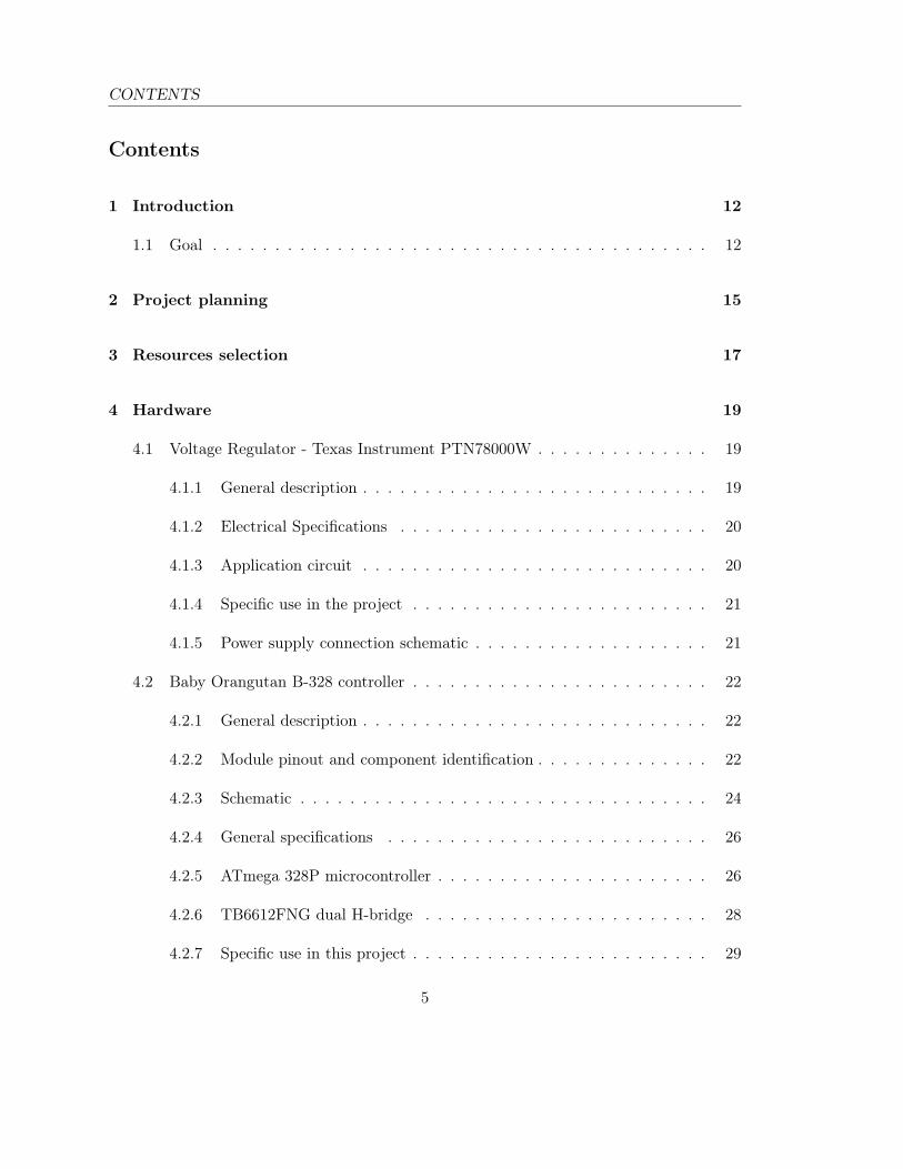
5.1 Car assembled
The figure 39 on page 65 illustrates how the car was finally packed, with every single sensorassembled into the car structure. In the back view picture, the magnets of the encoder canbe appreciated on the left back wheel. As it can be clearly seen, each track has differenttag sticked, so that the QTR sensor can detect when the car reach a new piece, as well aswhich sort of piece it is.
(a) Side view (b) Back view
(c) Front view (d) Top view
Figure 39: Car assembled
In addition, the figure 40 on page 66 shows a general and more graphic schema of thehardware interconnection in our system. This schema is more intuitive than the electric ones
65

5.2 World model - track pieces identification
showed trough the previous sections, and it illustrates the general picture of the hardwareconnection in the project.
Figure 40: Slot-car hardware connections in a graphic schema
5.2 World model - track pieces identification
The world model of our car is discrete. That is to say that, despite the fact that the numberof different possible track is significantly huge, the number of combinations is not infinite.Considering 6 different sort of pieces, the track can be built using any combination of thosepieces. In addition, every piece has its own tag, so that the QTR sensor can check overwhich kind of piece the car is going at any moment. The figure 41 on page 68 shows the 6different pieces, having each one of different characteristics:
1. Start: there is only one and it represents the beginning of the track. Furthermore,since the car goes over it once per lap, it has 2 different tags, so that the car cancheck if the side of the track where it is is the side that it actually believes that it is.
2. Straight: there are a considerable number of those tracks, it is the basic piece thatrepresents a track straight, so it only needs 1 single tag.
3. Swap: there is only one of this kind of track, and it creates for the car a mandatorychange of the side. It only requires 1 single tag.
66
5 CAR PACKED AND TRACK PIECES IDENTIFICATION
4. Switch: there are 2 of those kinds of pieces, and each one represents a possible side-change of the track, with the slight difference that one of them leads to a right to leftchange, and the other one to the opposite switch.
5. Curve: there are a considerable number of those tracks, it is the basic piece thatrepresents a track curve, so it only needs 1 single tag.
6. Funnel: there is only one of this sort of track, it creates a narrowing in the track,so the cars must be aware that a collision might be fairly possible if two cars get intothis part of the track at the same time.
7. Bridge pieces: Those are 2 straight pieces that allows the identification of a bridge.They are just simple straight pieces with different tags, so that using them in thebeginning and end of bridges, they can be identified easily1.
Likewise, the table 14 on page 69 illustrates the different tags used to identify the pieceson the track. It is of note the following characteristics:
1. The first and most important characteristic is that the code selection was no randomlydone. On contrast, different values were tried for different pieces, and the selectionwas done according to those codes that performed better on the specific pieces. Forexample, the code 0000102 was used for a long time for Swap pieces identification,but finally it had to be changed because in the Right Curves, which are identifiedby the code 000110, the car sometimes drifted, and as a result the QTR sensor read000010, getting a Swap identification rather than a Right Curve. Likewise, some otherwrong cases were studied, and consequently the codes were exchanged until the mostsuitable codes-pieces combination was found.
2. Two different tags are used in the SWITCH piece. That is because, it is required theidentification of whether the possible switch would take place from right to left orvice versa.
3. It is also remarkable that since the accelerometers don’t work, there is only one wayleft to identify the track bridges. So as to do that, two straight pieces with two specific
1The identification of the bridges with tags was required since the accelerometer induced such a greatnoise, that the identification of the bridge elevations was not possible with this sensor
202 in decimal
67

5.2 World model - track pieces identification
(a) Start (b) Straight
(c) Swap (d) Switch
(e) Curve (f) Funnel
Figure 41: Track pieces
68

5 CAR PACKED AND TRACK PIECES IDENTIFICATION
tags were used, the first one must be always included at the beginning of the bridge,and the second one at the end. These 2 codes are shown in the table.
4. One extra code is used for unrecognized tags 1.
5. As it can seen from comparing the table 14 and the tags on the figure 41, black colorsaccount for 1 logic, by contrast with white ones, which account for 0 logic.
That is mainly because a white color means that the respective capacitor in the QTRhas been discharged, and therefore, that the input of the sensor is at the same voltagelevel that ground. On the other hand, black color leads to a non-discharged state onthose capacitors, making possible a HIGH level reading on the QTR sensor.
PART BIN HEX DECUNKNOW 0 0 0 0 0 0 00 0
CURVE RIGHT 0 0 0 1 1 0 06 6START RIGHT 0 0 1 0 1 0 0A 10BRIDGE DOWN 0 0 1 1 0 0 0C 12
SWAP 0 1 0 0 0 0 10 16STRAIGHT 0 1 0 0 1 0 12 18
SWITCH LEFT 0 1 0 1 0 0 14 20FUNNEL 0 1 0 1 1 0 16 22
CURVE LEFT 0 1 1 0 0 0 18 24BRIDGE UP 0 1 1 0 1 0 1A 26START LEFT 0 1 1 1 0 0 1C 28
SWITCH RIGHT 0 1 1 1 1 0 1E 30
Table 14: Tag codes for piece identification
1Values that the QTR sensor reads, and which don’t match with any previously establish code
69

6 Project communications
6.1 General description
The communication procedure between the Baby Orangutan and the Wixel, which is locatedon the car, takes place through a serial communication. This Wixel transmits in turn thedata to the other Wixel via radio, which in a third step send the data to the computerthrough USB protocol. Similarly, a reverse communication (USB to radio, radio to serial)is also possible.
The three communications have a similar configuration, having the three of them a baudrateof 112500 kbps, with 1 stop bit and parity bit.
The main goal of this section is the description of the layer 3 and 5 of the OSI model usedthrough the communication described above.
6.2 Protocol definition
6.2.1 Packet syntax
The different data is sent using non-fixed length packets, which contains a START byte atthe beginning, as well as a STOP byte at the end of the packet, in order to enable this sortof transmission.
Moreover, the second byte of each packet establishes the sort of packets that is being sent,so that the receptor can know which kind data is acquiring, thus, this byte is known asthe order byte. Finally, a 8 bits CRC is located in the penultimate position of the packet.Since CRC stands for cyclic redundancy check, which is an error-detecting code, this bytepermits the receptor to detect accidental changes to the data.
All this configuration might been seen in the figure 42 on page 71:
70

6 PROJECT COMMUNICATIONS
Figure 42: Start - Stop bit Serial
6.2.2 Packet encoding
The main difficulty that the transmission described above may face is that the data bytesin the middle of the package could have the value of the START or STOP bytes, whichmight cause the receptor to read wrong the packet or to acquire only partial data of thewhole packet.
In order to solve that, every packet is checked before sending, and if any data byte fits withan START or STOP, an XOR operation is executed with this byte in order to mask it, anda third byte of control is inserted right before this changed byte, so that when the receptorreads the package and find a control byte, it knows that the next byte is encoded and thatthe control byte that it is reading should be ignored.
Since the data bytes can also have the value of this CONTROL byte, when the packetchecking takes place so as to mask the required bytes, not only the value of the STARTand STOP bytes are examined, but also the value of the CONTROL byte.
Finally, it is fairly evident that encoding them using a XOR operation allows the receptorto decode them using the same XOR operation.
The figure 43 on page 72 show this masked process:
6.2.3 Control bytes
According to the previous section, 6.2.2 - Packet encoding, every legal packet should haveat least the START, order, CRC and STOP bytes, as well as CONTROl bytes to mask anydata byte that matches with the value of the START, STOP or CONTROL bytes.
However, three exceptions to this rule were build in the protocol of this communication, one
71

6.2 Protocol definition
Figure 43: Control Serial
exception for each of the 3 control bytes that synchronize the communication or indicatewhether a good/wrong reception took place. These 3 bytes are described as follow:
1. SYN (0x16): It indicates that the Baby Orangutan is currently full initiated andthat it is ready to start communications.
2. ACK (0x06): It indicates that the last packet sent from the computer to the BabyOrangutan was received properly.
3. NAK (0x015): It indicates that the last packet sent from the computer to theBaby Orangutan was not received properly.
It is of note that, the flow direction of this 3 bytes only takes place from the car to thecomputer. The main reason for this is that the function of this bytes is to avoid data loss,and since the critical data is just the one sent from the computer to the microcontroller, onlythe checking in one direction is required. Furthermore, whereas implementing a functionthat takes care of data buffers and resend packets so as to avoid data loss is rather simplein the computer, it consumes a fair amount of resources in the microcontroller. That isexplained better in the next section, 6.3 - Data flow direction.
72

6 PROJECT COMMUNICATIONS
6.3 Data flow direction
It is immediately evident that the Baby Orangutan could send periodically packets to thecomputer with updated data without caring about whether a correct or wrong receptiontook place. That is mainly because since it sends data frequently, the computer would justhave to wait for the new updated sensor data to continue its control algorithm, and nogreat harm would occur.
On the other hand, when the computer sends a packet to the Baby Orangutan, the BabyOrangutan answers with an ACK or NAK byte to indicate a correct or non-correct reception(respectively) of the previous packet. That is required because the Baby Orangutan needsto receive speed commands and control data which are really important to be obtained,so if a wrong communication occurs, the computer should realize about that, and as aconsequence it ought to evaluate whether the better option is to send the same commandsor to build another packet with updated commands.
6.4 Serial channel communication
All the serial communication between the Baby Orangutan and the Wixel are managed bythe library Serial.c, developed and built specially for this project.
Taking into account the protocol described above, it is important to understand how thislibrary works, so that the serial communication is fully understood. Basically, Serial.c canbe divided into two different parts: the reception and the transmission of data bytes.
Looking closer at the reception, it is important to remark that this process starts with theinterruption routine of the reception in the serial channel. In this routine, the library readsevery byte that it arrives until it reads an START byte, moment when it knows that thenext incoming bytes are part of a whole package. After receiving this byte, the librarystorages the next incoming bytes until a STOP byte appears, when obviously the specificpackage is finished.
Once it has this raw package stored, the library checks every individual byte with theCONTROL byte, so that if some byte has this value, this byte is eliminated from thepackage, and the next byte is unmasked so as to have its proper value. In tandem with this
73

6.4 Serial channel communication
task, when the task compares the value of the bytes in the package with the CONTROLbyte, it also calculates and updates the CRC of the package with those values. Then, oncethis has been done, it checks if the CRC calculated for the library matches with the CRCvalue send at the end of the package. If the CRC matches then the package was well receivedand the library sends a ACK. By contrast, if the CRCs are different, there was a data loseand the library sends a NACK so as to ask to the computer for the same package.
Finally, if the CRC matches, the library checks the first byte of the package, evaluating therequest from the computer, and acting afterwards as a consequence.
In a second step it would be the data sending. In order to perform this task we considerthe fact that since several libraries in our program might try to send data at the same timeand the packages are quite long, it seems reasonable to use a buffer1. Basically, every timesome library wants to send a package, it must call the function SendPackage.
The function SendPackage gets the package, calculating its CRC firstly, and checking ifany byte of the package has the same value that START, STOP or CONTROL afterwards.In this case, the function masks the byte, and insert a CONTROL byte before this byte.Likewise, it inserts the START and STOP bytes in the package, as well as it stores the wholepackage once built in the buffer of transmission. Finally, it checks if the Serial Channelis not currently sending a message, in which case sends the first byte of the package. Bycontrast, if the Serial Channel is currently working, this function does not need to doanything, because it will be the own interruption routine of the Serial Channel which willtake care of sending the bytes inserted into the buffer.
Moreover, it is necessary to describe the routine that rules the interruption of the trans-mission of the Serial Channel. Every time this routine is executed, it firstly checks if theinterruption was done for a byte that is not in the end of a package. In that case, it knowsthat is currently sending a package, so that it sends the next byte within the transmissionbuffert. By contrast, once the routine is executed because the last byte of a package wassent (STOP byte), it checks if a ASK, NAK or SYNC response must be transmitted. Ifno one of those response must be done, then it checks if the buffer of transmission is notempty, sending the first byte of the next package if that is the case.
1The serial channel already has one, however it is only 8 bytes long, which is not enough for the lengthof our packages
74

6 PROJECT COMMUNICATIONS
Finally, it is remarkable that when a response must be transmitted, there is a specificroutine that in those cases updates a variable that indicates that a response must be doneas well as which kind of response it is. This variable is the same that is checked in theinterruption routine described above.
In order to acquire a better understanding of how all this library works, the flow diagramscan be seen in the section 17.1.10.
6.5 Wixels Communication
Since the Wixel is provided with a library to manage the wireless, USB and serial com-munications, those libraries where used to transfer the data from the Orangutan to theComputer, receiving the computer the data in the exact format that the Orangutan sendsit, and being the Wixel just a gateway in the middle of this communication.
Therefore, since those libraries where not built specifically for this project, there won’t bea great description of them.
6.6 USB communication
Despite the fact that the Wixel is connected with the computer through USB, it acts as avirtual serial port for the computer. Therefore, in order to receive the data from the Wixel,the computer uses the Python library pyserial.py to read the serial data receive from theBaby Orangutan through the Wixels.
The use of this library, as well as the interpretation of the received data will be discussedin the next section, section 9.3 - Computer serial communication - SerialCom Node, sincethat section illustrates how the data is received in the High Level in order to debug andtest the communication from the low level as well as the configuration of the sensors.
6.7 Orders
As it was stated before, the second byte of every packet defines the package that is beingsent, so that the receptor always know what kind of data might expect from this packet.
75

6.7 Orders
First of all, it is important to note that the sort of packages sent by the computer to the carare different than the kind of packets sent in the opposite direction. Therefore, the ordersbytes that the computer can use will be described first:
1. S: The computer tries to change the system state, so that the package contains thenew system status and mode.
2. M: The computer wants to change the car speed, so that the package contains thenew PWM cycle.
3. m: The computer asks for the speed value, so that the rest of the package is justthe CRC and the STOP byte.
4. I: The computer sends the initialization vector, thus, the rest bytes will indicate thenew system state, the LED frequency, as well as the period of the four sort of reports.
5. r: The computer asks for a sensor report, so that the rest of the package is just theCRC and the STOP byte.
6. u: The computer asks for a IMU report, so that the rest of the package is just theCRC and the STOP byte.
7. s: The computer asks for a system state report, so that the rest of the package isjust the CRC and the STOP byte.
8. p: The computer asks for a PID report, so that the rest of the package is just theCRC and the STOP byte.
In the orders described above, it can be seen how, despite to the fact that the reports aresent with specific periods, the computer might also ask for those reports under requests.That implementation was done for debugging purposes.
Regarding to the orders which the car sends to the computer, the list below describe all ofthem:
1. m: The car sends the speed value, so that the rest of the package is just the PWMcycle in the car.
76

6 PROJECT COMMUNICATIONS
2. r: The car sends the sensor report, so that the rest of the package contains theencoder value, the time between the encoder measures, the gyroscope, and a tagvalue with the time between tag readings if the car has read a tag.
3. u: The car send the IMU report, so that the rest of the package is the 9 values ofthe 3 sensors of the IMU.
4. s: The car sends the system state report, so that the rest of the package containsthe system status, mode as well as car speed.
5. p: The car sends the PID report, so that the rest of the package is the reference,error, actuation, proportional part and integral part of the PID.
6. t: The car sends the tag values of the a new track, so that the rest of the packagecontains the sequence of tag values that the car has read in the EXPLORING mode.
7. ACK: It is the only byte in the package.
8. NACK: It is the only byte in the package.
9. SYN: It is the only byte in the package.
77

7 Low level programming
In order to acquire the data of every sensor, as well as control the motor speed, low levellibraries were built using C programming language. First of all, and before assembling allthe hardware in the car, small and independent programs were designed to check the properfunction of the whole hardware and they communication with the Orangutan controller.Once this task was done, the next step was built the previously mentioned libraries, in orderto establish a efficient system in the low level, and test all those libraries in the assembledcar.
7.1 Low level libraries definition
7.1.1 Array.c
This is the library that takes care of the reading of the QTR sensor. In order to performancethis task, this library configures and uses the Timer 1 interruption of the Orangutan.Concretely, it establishes two different time steps with two different goals:
1. In the first one, the library sets the QTR ports as inputs so as to read the port, andthen it sets the Timer 1 interruption for the threshold of 200µs required to distinguishblack from white.
2. In the second one, executed in the Timer 1 interruption of 200 µs, the library readsthe QTR ports, then it sets the QTR port as outputs with logic ones, so that thecapacitors of the QTR are charged, and finally it configures the Timer 1 with theminimum time to charge the capacitors again.
In the second step mentioned before, the library calls a function that takes care of thevalues that are read. Basically, this function receives tag values, and ignores all of themuntil it receives the first value that is one of the valid and used codes. At this point, a burstof readings is performed, so that the function storages the next tag values that it receives ifthey are valid values. It does this task until it gets a tag value of all blacks, moment whenthe QTR has left the tag and is currently reading only the track surface.
78

7 LOW LEVEL PROGRAMMING
Then, after that stage, the truly value of the tag is calculated as the most repetitive valuewithin this burst. As a result, bad readings are avoided, since every tag is read severaltimes, and only valid values are considered, so at the end, even when the sensor might readsome wrong values, most of the readings of a tag would be right, and consequently, themost repetitive value would be the real value of the tag.
Moreover, if the value read is not one of the defined values, the reading is omitted andno value is sent. However, if there is a proper value the new tag value is available for themicrocontroller. Finally, this new value would be evaluated for another library, which takescare of the system actions after a tag reading depending on the car mode. This library iscalled Control.c, and is described in the section 7.1.3.
The section 17.1.2 illustrates the flow diagram of this library, with such diagram the 3functions of this library can be better understood.
7.1.2 Status_control.c
This library manages the different car status, checking if there is any status change, andacting in consequence. In order to be executed, the Main.c calls the library entry periodi-cally. It is of note that, the slot car has 5 possible different status, status that may changeeither because the computer in the high level sends the right order, or because the owncurrent status requires a status change.
1. OFF: the car is stopped, and there is no motion. A direct order from the high levelis necessary in order to change this status.
2. EXPLORING: the car is reading tags and trying to build the track map. Onceit reads the start tag for a second time, it knows that it has driven a whole lap, soas a consequence, it can check the sequence of the track pieces that has been readchanging the status to CHECKING MAP. The computer has to order the car to startthis status.
3. CHECKING MAP: once the car has done one lap, this status checks that thesequence of different pieces that have been read creates a closed circuit. If the resultof the checking is negative, the car has either missed one tag or read one tag wrong,
79
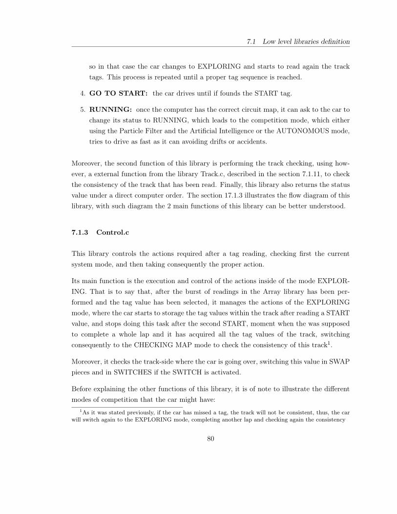
7.1 Low level libraries definition
so in that case the car changes to EXPLORING and starts to read again the tracktags. This process is repeated until a proper tag sequence is reached.
4. GO TO START: the car drives until if founds the START tag.
5. RUNNING: once the computer has the correct circuit map, it can ask to the car tochange its status to RUNNING, which leads to the competition mode, which eitherusing the Particle Filter and the Artificial Intelligence or the AUTONOMOUS mode,tries to drive as fast as it can avoiding drifts or accidents.
Moreover, the second function of this library is performing the track checking, using how-ever, a external function from the library Track.c, described in the section 7.1.11, to checkthe consistency of the track that has been read. Finally, this library also returns the statusvalue under a direct computer order. The section 17.1.3 illustrates the flow diagram of thislibrary, with such diagram the 2 main functions of this library can be better understood.
7.1.3 Control.c
This library controls the actions required after a tag reading, checking first the currentsystem mode, and then taking consequently the proper action.
Its main function is the execution and control of the actions inside of the mode EXPLOR-ING. That is to say that, after the burst of readings in the Array library has been per-formed and the tag value has been selected, it manages the actions of the EXPLORINGmode, where the car starts to storage the tag values within the track after reading a STARTvalue, and stops doing this task after the second START, moment when the was supposedto complete a whole lap and it has acquired all the tag values of the track, switchingconsequently to the CHECKING MAP mode to check the consistency of this track1.
Moreover, it checks the track-side where the car is going over, switching this value in SWAPpieces and in SWITCHES if the SWITCH is activated.
Before explaining the other functions of this library, it is of note to illustrate the differentmodes of competition that the car might have:
1As it was stated previously, if the car has missed a tag, the track will not be consistent, thus, the carwill switch again to the EXPLORING mode, completing another lap and checking again the consistency
80

7 LOW LEVEL PROGRAMMING
1. AUTONOMOUS: the car drives without the computer help, taking just into ac-count the value of the tag that it reads, so that it knows in which kind of piece itis, and can set a speed according the sort of piece is trying to cross. This mode wasthough in case of computer failure, since it provides the car a easy and quick solutionfor racing if the computer stops the communication.
2. SLAVE: the car drives using the speed reference that the computer provides, in-serting this reference in the PID and getting as a result the motor actuation.
Taking that into account, It is of remarkable that this library also control the car speedaccording to the kind of piece that it reads in the AUTONOMOUS mode.
The section 17.1.4 illustrates the flow diagram of this library, with such diagram the 4 mainfunctions of this library can be better understood.
7.1.4 Eeprom.c
This library takes care of storing system data, such as reference speed or configurationparameters, in the EEPROM memory of the microcontroller. This is required because thecircuit suffers lose powers due to the mechanical-electrical connections of the track, andwith each lose power the communications need around 500 ms to be restarted, so a quickreading of the previous parameters is needed to allow the car drive right after the lose powerand not with the direct order from the computer after the 500 ms.
Moreover, it is required the recovering of the car status before the power lose, and sincewhen the car is restarted it gets the state after being programmed, storing the status valueon the EEPROM, and reading them afterwards, it is a simply and great implementation toperform this task.
Furthermore, and since this library storage all the parameters of the system, the samelibrary updates the variables that represent these parameters at the same time that itstorages them in the EEPROM. That is done because both process are supposed to beexecuted one right after the other, so that doing both task inside the same library is moreefficient.
81

7.1 Low level libraries definition
Finally, the most powerful tool of this library is how it manages the writing in the EEPROMmemory. First of all, it is of note that the interruptions of the µController have no priority,so that once one has started the rest of them must wait for the first one to finish beforea second one might start. Due to that, writing in the EEPROM is a critical task: ittakes a really long time and most of the system parameters are update inside µControllerinterruptions. As a result, if the writing is performed also inside of interruptions, the longtime required to do that might cause a retard on the execution of the other interruption,which could lead to serious problems in our system since the execution of several processes,such as the PID or the tag readings, must be done on real time.
In order to solve this problem, every time a parameter must be updated, this librarystorages it in a buffer, saving the data to be written as well as the EEPROM address whereis supposed to be storage. This buffer is then read in the Main.c, out of any interruption,and is the Main program the responsible for taking out data from the buffer and storageit in the EEPROM. That way, having a region of the EEPROM for every parameter, thestorage of the system data in the EEPROM can be performed out of any interruption.
The section 17.1.5 illustrates the flow diagram of this library, with such diagram the severalfunctions of this library can be better understood.
7.1.5 IMU.c
This library manages the reading of the accelerometer, magnetometer and gyroscope in theIMU sensor. In order to do that, it uses the TWI protocol described on the section 4.6.3.Before the execution of the readings, it also configures the three Slaves in the most suitableway.
Basically, the entry of this library is the interruption of the TWI, interruption executedright after any activity in the channel, so once the Slave are configured, the Orangutansends a START signal in the channel, so that the interruption is executed the first time.
From the execution of the interruption of this routine, the main function of this library iscalled. This function executes and manages the sequence of actions required to read thedata of the different devices. The communication and process to read the data from oneSlave can be seen on the figure 44 on page 83.
82

7 LOW LEVEL PROGRAMMING
MASTER | ST | SAD+W | | SUB | | SR | SAD+R | | => SLAVE | | | SACK | | SACK | | | SACK | => |(1) | (2) | (3) |(4) | (5) | MASTER => | | MACK | | MACK | | MACK | => SLAVE => | DATA | | DATA | | DATA | | => | (6) | (7) | (8) | MASTER => | | MACK | | MACK | | NMACK | SP | SLAVE => | DATA | | DATA | | DATA | | | | (9) | (10) | (11) |(12)|
Figure 44: TWI packages to read one slave
It can be seen how first of all, the Master send a START signal + the Slave address |writing order, and once the Slave acknowledges it, the Master send the command to readthe specific register of the slave with auto-increment, so that pointing at the first registerthat contains the data measures of the Slave, the reading of the following registers, whichcontain the remaining data measures, is done automatically. After the Slave acknowledgesthe command, the Master send a START + the Slave address | reading order, so now theSlaves knows that it must send the data in the register previously specified for the Master.Moreover, since the Master specified the auto-increment, the Slave sends the data in thefollowing registers until the Master stop acknowledging the reception, process done rightafter receiving the six bytes of the Slave.
Once the function finish the readings of one Slave, it switches the communication to thefollowing Slave, repeating the same process described above.
Moreover, it is of note that the first action the interruption routine does is checking if theTWI status is the expected status. In that case, the routine executes the main routine ofthis library. By contrast, if the status differs, the interruption routine updates the datavariables of the current Slave to 0, stops the communications, and sends a START signalso that the communication with the next Slave can start. Likewise, the expected Status isa variable updated in the main function of the library right after any command has beenexecuted on the TWI channel.
83

7.1 Low level libraries definition
The section 17.1.6 illustrates the flow diagram of this library, with such diagram the inter-ruption routine and the main functions of this library can be better understood.
7.1.6 Main.c
This library is responsible of the coordination of the other libraries, constituting the maincore of the low level program.
It first task is the initialization and configuration of every sensor, the reading of the EEP-ROM memory in order to restore the last configuration to the car, the initialization of thePID and the communications, as well as the initialization of the watchdog timer.
Once this task has been done, the Main program executes a closed loop where, the firstactions is the re-initialization of the watchdog, so that the program has a security measurethat in case of failed execution, the µController is always re-initialized after a certain time.
The second task is the management of the EEPROM writing. So as to do it, inside the loopthere is a call to a secondary function, function that checks the EEPROM buffer, so that ifthe buffer has data, the function takes out the first data with its address, and tries to writeit on the EEPROM memory. Doing this process, any interruption can be executed in themiddle of a writing, so that the EEPROM writing doesn’t penalize the execution of anyinterruption of the real time system. It is of note that the functionality of the buffer is likea FIFO memory, where the first data in, is the first data out, so the writing is performedin the same order that the different libraries ask to write data in the EEPROM.
The third task of this loop is a call to the library control_status(7.1.2), which as it wasstated before, checks if there was any system status change, and it takes the proper actionsas a result.
Finally, the loop calls the functions that executes the time base of the system, which using avariable, which is updated in the interruption of the Timer 0 and that storages the numberof pulses executed for the timer 0, can control when the number of pulses of the timer 0 isequivalent to 10 ms, creating consequently the time base based on a 10 ms period, being10 ms chosen as the minimum period that can guarantee a proper execution of the PID.
The requirement of the data base was needed because there are several resources that
84

7 LOW LEVEL PROGRAMMING
require real time, and unfortunately there are no enough timers to attend all those resources.Moreover, this way of create the time base was designed because the timer 0 manages theled frequency, and since this frequency varies according to the port track used for the SwitchHardware, the interruption of the Timer 0 might be executed with four different periods,so it is not possible to create the time base based on the number of executions of the timer,and therefore, the simplest solution is to count the number of pulses of the timer since thefrequency of those pulses is constant.
Considering everything stated in the two last paragraphs, the function time base is executedevery 10 ms, period chosen as the PID base. Therefore, this function gets the value of theEncoder and Sharp values with this period and executes the PID function afterwards. Then,it updates the exactly time between the sensors report, which is required so that the HighLevel has a precise measure of the encoder measurement intervals, and then the motionmodel is more accurate. Moreover, it is also responsible for checking after the initializationof the car if the Wixel and the IMU are ready. In order to do that, it waits the requiredminimum time using a counter, and after that it sets the variables that let the IMU andWixel be operative.
It is also of note that, since the car can send to the computer four different data reports:PID, IMU, sensors (with just the specific data for the Particle Filter) and system status,it seems reasonable to make configurable the period of those reports. As a result, thecomputer can choose between five different periods for every report, and those periods aremultiples of 10 ms, so that with a counter for every report, inside the time base functionit can be checked when a specific report must be sent, and consequently, it can create thespecific package a call the routine of the Serial.c library to send this package.
Finally, the Main.c also contains a routine for a complete initialization of the car. Thisroutine was required to implement the functionality that the computer can configure witha single package the period of the four reports, the system status and mode or the frequencyof the infrared LED. Furthermore, the interruption vectors, which in turn make the call tothe specific interruption functions in the specific libraries, are also defined in the Main.clibrary.
The section 17.1.1 illustrates the flow diagram of this library, with such diagram the thefunctions of this library can be better understood.
85

7.1 Low level libraries definition
7.1.7 Motor.c
This library has several different tasks, most of them directly related with the managementof the car speed.
1. Using the Timer 0 of the microcontroller, it manages the variable that rules thetime base executed in the Main.c. Moreover, the execution of this interruption isprogrammed according to the period required to power the infrared LED for theSwitch piece, so that the output of the port that rules the LED is varied in everyinterruption. Then, taking into account the number of pulses of the Timer 0 executedbetween interruptions1, it updates the variable for the time base as well anothervariable that takes care of the time between the reading of two tags2.
2. It checks if the Hall sensor output has changed, in which case it increments thevariable that storages the encoder value. Then, in the routine of the time base, thefinal encoder is used and re-initialized.
3. It manages the initialization of the TB6612FNG dual H-bridge, which takes care ofthe motor power.
4. It modify and read the output values of the TB6612FNG under specific request fromthe high level. That function is useful for debugging purposes since the normal outputvalues for powering the motor come from the PID library.
For a better understanding of this library, the section 17.1.7 illustrates the flow diagram ofthis library.
7.1.8 PID.c
This library manages the PID control for the car speed. Since it is a key part of the project,and its designing and testing was done in a posterior step, the operation of this library willbe discussed later on, in the section 8 - PID designing and programming.
Moreover, the flow diagrams of this library can checked on the section 17.1.8.1This number depends only in the LED period2Time required for the posterior implementation of the Artificial Intelligence
86
7 LOW LEVEL PROGRAMMING
7.1.9 Sharp.c
This library manages the Analog - Digital conversion of the voltage values of the Sharpsensor. Using a continuos conversion mode, it produces every 13 µs a new A/D conversion,updating in turn the variable that storage the Sharp sensor data, and which can be read bythe microcontroller. Furthermore, it also has defined the function that can build a packagefor the Sharp value, and send it. This function was build with debugging purposes. Theflow diagrams of this library can checked on the section 17.1.9.
7.1.10 Serial.c
This library manages the Serial communication between the Wixel and the Orangutan.Since it is also a key part of the project, the operation of this library was already discussedin the section 6.4 - Serial channel communication.
Furthermore, the flow diagrams of this library can be checked on the the section 17.1.10.
7.1.11 Track.c
This library check the consistency of the track map when the car is in the status CHECKINGMAP. Using and considering the specific geometry of every piece of the track sequence, itpropagates the initial coordinates of every piece that forms the track, so that it can checkthat, when a START tag is read for a second time, the coordinates of the piece of the secondSTART are the coordinates of the piece of the first START. In that case it knows that thesequence of pieces build a proper circuit.
Moreover it also has a function that creates the proper package to send that representsthe new track that has been found in the EXPLORING mode. The flow diagrams of thislibrary can be checked on the the section 17.1.11
87

8 PID designing and programming
Setting the speed of the car had a problem, and it was that the motor supply was setadjusting the cycle of the PWM output on the TB6612FNG dual H-bridge (section 4.2.6),thus, the power supply for the same PWM cycle might vary according to the power supplyof the own track and according to other parameters such as the level of dirt in the track orde angle of the car when it is racing.
In order to solve that, we thought that the speed setting might be done according to thespeed itself, not as a indirect value through the cycle of the PWM output. Therefore, andsince we had a direct value of the car speed on the encoder, it was fairly evident that havingas reference the number of ticks in the encoder, the PID error might be easily calculatedwith this reference and the encoder measure, and with this error the PID output as thePWM cycle.
8.1 PID designing
Either in the case where the High Level states the car speed, or in the case where thecar is running in the autonomous mode, the speed reference is stated as a PWM cycle.Thus, in order to establish a invariable relation between the PWM cycle and the encodernumber of ticks, we studied this relation with the car running in straight pieces and thetrack completely clean, and we came up with a function that could switch PWM cyclevalues and encoder number of ticks under this conditions.
Using this function as basis of our control, every time the PID receives a PWM cycle, itswitches this value to the respectively number of encoder ticks. Then, the PID can easilycalculate the error as the difference between this reference in encoder ticks and the actualencoder value.
Then, using the proper constants for the integral, proportional and derivative part, anoutput in the range of the PWM cycle is obtained, and the car speed is set in every part ofthe circuit as if the car were running in straight lines and without dirt.
The assumption of straight and without was done because those are the optimum conditionswhere no interferences are making the car slow down.
88

8 PID DESIGNING AND PROGRAMMING
The dt chosen was 10 ms, because it produced a perfectly trade off between a great speedcontrol and the time consumed to executed periodically its code.
Furthermore, the encoder reference has continuous values, and the encoder measure onlydiscrete values1, thus, the encoder is constantly oscillating in the range of reference ±1 ticksince it can never reach the proper real value. Sometimes, the values of the encoder canalso oscillate in the range of the reference ±2 ticks, since 10 ms is a really tiny time periodto measure the exact ticks accurately.
As a consequence, the designing of the PID was done taking into account that we had areally fast system, where the error in the stable position was constantly oscillating betweennegative and positive values in the range of ±1. Due to that, the derivative part of thePID was not modeled and used for not being appropriated for our fast system. Moreover,in order to balance the actuation of the proportional and the integer part, we realized thatdue to this magnitude of oscillations in the error, the proportional part by itself leaded toa great oscillations in the amplitude of the actuation. As a result, we modeled the integerpart in order to trade off this oscillations, creating a smother actuation.
Consequently, the final result was a PID which part of the work was done with the propor-tional part, which creates an output with a high amplitude variance but makes the responseof the PID faster enough, and part of the work is done by the integral part, which reducesthe oscillations of the proportional part but makes the system a bit slower, though notslower enough as to make the response of the proportional not able of balance this slowresponse. As a result, the PID creates fast and accurate speed responses, even when thenatural behavior of the car is slow down, like in curves.
The figure 45 on page 91 illustrates the behavior of the PID. It can be observed thatwhereas the reference (red line), is a straight line within real values, the encoder value (pinkline) oscillates over and under this reference, normally in the range of ±1 tick, with somesporadically ±2 ticks, creating the same oscillation in the PID error (blue line). However,it can be seen how the average of the encoder ticks actually follows the reference properly,and the average of the error is 0.
Moreover, it can be how the in the first speed change, the acceleration between 0 and 5 ticksper 10 ms, the PID response is fairly fast, reaching almost immediately the state required.
1Whereas the reference is a real number, the real encoder value is a integer value in the range of 0-20
89

8.2 PID testing
Likewise, when the car has to brake between 5 to almost 3.5 ticks per 10 ms, the answer iseven faster.
The whole functionality of the PID is illustrate through the flow diagrams of the specificPID library, which can checked on the section 17.1.8.
8.2 PID testing
In order to analyze the response of the PID, the PID values were sent to the computer, sothat representing in a graph the different data, we could test different constants so as toobtain the constants that produced the best performance.
The figure 45 on page 91 shows the response of the PID with the definitive values that wechose.
90

8 PID DESIGNING AND PROGRAMMING
(a) PID response
reference↔ red | encoder ↔ pink |error ↔ blue
(b) PID response in a closer detail
Figure 45: PID simulation
91

9 High level for serial communication and debugging purpose
The high level, which contains a Particle Filter for car localization as well as an ArtificialIntelligence, was built using Python (programming language) as well as the software ROS(Robot Operating System) to create the different processes and to represent the car simu-lation using its specific software RVIZ. Therefore, the main goal of this section is illustratethe first steps using Python and ROS in order to create the serial communication and todebug the sensor data, leaving the description of the designing of the Particle Filter andthe AI for later sections.
9.1 Glade software
In order to create the GUI which gives access to the car configuration, or allows the execu-tion of the threads in ROS, the software Glade was used.
An example of a Glade interface can bee seen on the figure 46 on page 97 or on figure 47on page 98.
9.2 ROS software
ROS, or Robot Operative System provides libraries and tools to help software developerscreate robot applications. It provides useful tools such as hardware abstraction, devicedrivers, libraries or a 3D-simulation visualizer.
The main reasons for using this software is that it permits an easy implementation ofdifferent processes with their respective communications. This characteristic is really usefulin our project where different applications must be executed (GUI, particle filter, serial datamanagement, artificial intelligence, etc.), so organizing them as different processes insteadof threads helps to reach a better and faster program execution, since different cores mightbe used in double-cores CPUs.
Furthermore, another chief reason for using ROS is that it has integrated some simulationtools really useful for debugging and for the car representation. For instance, ROS hasintegrated a software called RVIZ, which allows an easy simulation of the car and the track,
92
9 HIGH LEVEL FOR SERIAL COMMUNICATION AND DEBUGGING PURPOSE
as well as the particles in the particle filter. The use of this simulation will be discussedlater on on the section 10 - RVIZ simulation implementation.
Basically, ROS has packages as the software organization unit of its code, where eachpackage might contain libraries, executables, or other elements. One of the most strikingfeatures within a package are nodes, which are executable files within a ROS package, butwith the great advantage that they can use some specific ROS libraries in order to createa communication with other nodes in a efficient way.
In other words, so as to communicate with other nodes, a node can publish or be subscribedto a Topic. A ROS Topic is a publisher-subscriber communication, where only one nodemight be publisher and other nodes can be subscribed to the information published. How-ever, every piece of information published must have a particular format, the format of thedifferent sort of information are defined inside of the message files within the package.
Likewise, nodes can use services to communicate with each other. But instead of publishinformation, services allow nodes to send a request to another node and receive a response.
Thank to those characteristics, all the high level applications were built, integrating ROS,python and Glade.
9.3 Computer serial communication - SerialCom Node
As it was stated in the section 6.6 - USB communication, Python has a specific librarycalled pyserial, which allows the management of serial data through a virtual serial port.This library detects virtual ports connected to the computer, as well as it builds buffers forsending and receiving data through those port.
The management of the serial communications was built integrating the different functionsof the pyserial library inside of a ROS node called "SerialCom". This node uses the libraryfunctions for receiving and sending data in order to create the communications with theWixel.
Furthermore, it publishes all the data it receives in a specific ROS topic, which can beaccessed by the other ROS nodes which need the car information (Particle Filter, AI, etc.).Likewise, it is subscribed to a Topic where other nodes can send information to the car, so
93

9.3 Computer serial communication - SerialCom Node
that every time this serial node detects a new publication on this Topic, it reads the data,sending it to the car in the proper format. The next sections will explain more detailedthose concerns.
9.3.1 Data reception
Firstly, it is important to note that this node uses two different python threads. The firstone for managing the data reception, and the second one for the data sending.
In the first thread, the node checks regularly the Wixel port, and when it detects a newpacket, it reads the whole package (taking into account the START and STOP bytes), andthen, it checks the existence of masked bytes unmasking them afterwards, before examiningthe CRC to check if the package is completely OK.
Once this step was done, the thread look at the kind of package it has received, and it buildsa specific package to be published on a ROS topic. Basically, since the car sends sensorinformation, information about the car status, information about the PID and about thetrack, this node publishes in 4 topics, one topic for each kind of information. Since eachROS node requires a different kind of data, this separation can been done, and consequently,a modular data transfer can be used.
1. The first ROS topic, uses a defined messaged with variables for the IMU sensor,encoder, Sharp sensor and QTR value. This sort of message is later published inthe topic where all the nodes needing the sensor information can be subscribed. Inaddition, it adapts the sensor information to readable values for the other topics. Forinstance, it changes the IMU data, which is just a number between -215 and 215, tothe proper data unit according to the sort of sensor (for example, to m/s2 for theaccelerometer).
2. In a second topic, it publishes a message with variables for the car status and the carmode.
3. In a third topic it publishes the values of the low level PID, which are needed to debugit in the high level using some ROS simulation tools.
94

9 HIGH LEVEL FOR SERIAL COMMUNICATION AND DEBUGGING PURPOSE
4. The fourth one takes just care of the tag sequence, which will lead to the constructionof the car track in the RVIZ simulation tool. As a consequence, this topic is usedat the beginning, when the car identify the circuit and sends that information to thecomputer.
9.3.2 Data sending
Using second thread, the node is subscribed to a ROS topic where other nodes can publishspecific data about the car speed and the car status/mode.
When a new data is published in this topic, this thread builds the package in the rightformat (that is to say that it builds it using the START, STOP, CONTROL, ORDER andCRC bytes).
Finally, once the packet is in the right format, the thread sends it through the virtual serialchannel using the specific pyserial library function.
9.3.3 Buffers management
In order to avoid data loss, as well as to create a good management of the data send-ing/receiving, 3 python queue were used as data buffers.
1. The first buffer takes care of the data that is supposed to be sent. Every time thesending thread needs to send a message, it insert the packet in this queue, and whenthe port is ready and available to send data, another function inside the same threadtakes care of the sequently sending of the individual bytes of those packets.
2. In a second queue, all the data received is storage, so the receiving thread can alsoexamine it sequently, avoiding any data loss.
3. In a third queue, all the data sent is stored, so that using the NACK and ACK carcommands, the data that has been previously sent can be send it again in case of awrong car data reception. In other words, when a ACK is received, the first packetinserted in this queue is erased. By contrast, when a NACK is received, the first
95

9.4 High level application
packet inside the queue is sent again, since that a NACK means that the car couldnot read this packet properly.
9.4 High level application
A GUI interface was created using the Glade software. The first feature of this GUI isthat acts as a security check. In other words, using a function of pyserial which examinesthe ports connected to some device, a security check was built in order to detect whenthe Wixel is connected, so that the user can only have access to the functionalities of theapplication as long as the Wixel is connected to the computer, avoid any sort of programexecution unless the Wixel is ready.
Once the program detects the Wixel connection, the user can open the communications,starting the execution of the "SerialCom" node, as well as check the different functionalitiesof the program. This sequence can be observed on the figure 46 on page 97.
9.5 Data debug
In order to test the accuracy of the different data of the car sensors, the proper readings ofthe tags on the track, the correct modifications of the car status and motor speed, as wellas its proper message format inside ROS topics, secondary windows were built as part ofthe GUI. Those windows can be seen on the figure 47 on page 98.
With the first GUI (figure 47a), the correct data on the sensor topic was examined. Whereasthe data of the Sharp sensor, the encoder and the gyroscope seemed to have proper values,the accelerometer and the magnetometer values seemed either, to have a lot of noise or tobe out of the range value that they were supposed to be.
In order to examine that problem in more detail, we used one package, that ROS hasincorporated, which can build graphs to represent the different data published inside theROS topics. The next two sections will examine separately both, the problem with theaccelerometer and the difficulty with the magnetometer.
96

9 HIGH LEVEL FOR SERIAL COMMUNICATION AND DEBUGGING PURPOSE
(a) Wixel is still not connected
(b) Wixel recognized and communication ready to be launch
(c) Communication opened and functionalities ready to be used
Figure 46: Communication start sequence97

9.5 Data debug
(a) GUI for collection data from every sensor but the QTR
(b) GUI for collection tags data and modify car speed
(c) GUI for manage the car status and mode
Figure 47: Debugging GUI
98

9 HIGH LEVEL FOR SERIAL COMMUNICATION AND DEBUGGING PURPOSE
9.5.1 Accelerometer debug
Looking at the accelerometer data in a graph, we detected that the noise in the accelerom-eter had 2 different sources. The first one it came from the car motor, which inducedvibrations on the PCB, transmitting those vibrations to the IMU, and consequently to theaccelerometer. The second one were vibrations from the track: since the car runs on aplastic track which can not be sticked to the ground, the track vibrates when the car drivesover it, leading to a vibration propagation through the car, and as a consequence, to theaccelerometer.
The representation of the accelerometer data can be seen on the figure 48 on page 100.
Firstly, in the first graph (figure 48a), it is shown the accelerometer data when the motoris off in the axis Z, it is immediately clear how in this situation, the noise is inexistent andthe acceleration in the Z axis is approximately the gravity acceleration.
By contrast, the second one (figure 51b) illustrates the accelerometer data in the same axiswhen the car is running on the track. Despite the fact that this value is supposed to beapproximately 9.8 m/s2 as the car is running over a flat surface, it can be seen how thenoise from the motor and the track is disturbing the correct values of the accelerometer,being of note that the noise value is almost ±3 times as many as the proper sensor value.
In order to solve this problem several techniques were tried:
1. First of all, we tried to filter the signal. The problem was that since the vibrationnoise appeared in a really wide range of frequencies and with a value treble than thetruly value, all the different filter that we tried failed. Whereas some of them couldfilter the signal, others produced an output too slow to be implemented.
2. As a second measure, we tried to isolate the noise. So as to do this isolation, we sep-arate the PCB from the car chassis using small rubber seals. However, the vibrationwere strong enough as to propagate through the rubber.
3. As a third technique we tried to build the track in different floors and stick the piecesto them, trying to eliminated the vibration from the track, which was greater thanthe motor vibration. However, that was useless because the vibration didn’t evenmitigated.
99
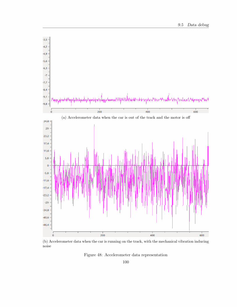
9.5 Data debug
(a) Accelerometer data when the car is out of the track and the motor is off
(b) Accelerometer data when the car is running on the track, with the mechanical vibration inducingnoise
Figure 48: Accelerometer data representation
100

9 HIGH LEVEL FOR SERIAL COMMUNICATION AND DEBUGGING PURPOSE
4. Finally, we tried to uncouple the IMU from the PCB using wires. Nevertheless, wecouldn’t find any other stable position for the IMU onto the car, so at the end, locatingit in the PCB was the only option.
In conclusion, as much as we tried, we didn’t come up with a solution to mitigate oreliminate the accelerometer noise. However, we could manage to create the particle filterwithout it, using the tags along the track as well as the own track geometry. That will beexplained later on, in the section 12 - Particle filter design and implementation.
9.5.2 Magnetometer debug
Examining the magnetometer data in a graph, we detected that the magnetometer not onlyhad noise, but it also showed values far greater than the Earth magnetic field. Consideringthat, we realized that some external magnetic field should be causing such value distortion.
First of all, we tested the car in different environments, however, the magnetic field stillremained affecting, causing noise in the magnetometer.
After that, we checked all the car hardware, and was at that point when the encodershowed up as the source of our problems. Since the encoder used 20 small magnets, themagnetometer couldn’t read properly the value of the Earth magnetic field. Instead, it wasdetecting the value of those magnets, being what we though as at first glance as noise justthe variations of the magnetic field when the wheel was turning1.
The representation of the magnetometer data can be seen on the figure 49 on page 102.It is immediately evident that despite the fact that the magnetic field on the Earth isapproximately 0.65 gauss, the values showed on the 3 axis (each color accounts for a differentaxis) are far greater, recording at values almost 15 times as high as the maximum value.
At this point we had to choose between the magnetometer and the encoder. Taking intoaccount the future requirements of the particle filter, we decided that the encoder was moresuitable, since the magnetometer could be replaced by the measures of the gyroscope or thegeometry of the track. However, it is not the goal of this section to explain the particle filter,that will be discussed later on, in the section 12 - Particle filter design and implementation.
1turning as a consequence the magnets too, changing constantly the magnetic field
101

9.5 Data debug
Figure 49: Magnetometer data with the noise from the encoder
102

10 RVIZ simulation implementation
10.1 General overview
As we have stated before in the section 9.2, ROS has integrated one simulation tool calledRVIZ, which simulates in a 3D graphic space the representation of robot movements, robotenvironments, and some other graphic forms such as spheres, points, lines, etc.
One of the graphic units that can be represented in RVIZ is a Marker. Markers constitutesa specific ROS message (visualization_msgs/Marker or visualization_msgs/ MarkerArray)and are at the same time instances of the predefined ROS class Marker or MarkerArray(the difference between the 2 messages is that in MarkerArray you can insert a group ofMarkers so that their rendering is faster and easier). In other words, defining in python aMarker means write the value of some object properties, which are at the same time thefields of a specific ROS message.
Is is quite evident that as we create those graphic units as ROS messages, they are repre-sented on RVIZ publishing those messages on a specific ROS topic.
10.2 Project elements design
The main and most useful characteristic of Markers are that they allow the representationof STL figures, being STL (Standard Tessellation Language) a file format used to represent3D CAD models in stereolithography and other solid freeform fabrication technologies.Thanks to this characteristic, using a 3D designing program we could create the differentpossibles pieces of the track, as well as the model of a slot car. Moreover, using the Markerto represent spheres, we represented the model of the particles for the particle filter.
In order to design the different pieces of the track, the software FreeCAD was used, so thatconsidering the geometry and the dimension of each track piece, every part of the track wasdesigned as a STL figure. The figure 50 on page 104 shows the design of the Swap and theSwitch.
By contrast, despite we did small modifications on the car figure, the main structure of thisSTL figure was obtained as a RVIZ resource and not as our own designing on FreeCAD. A
103

10.2 Project elements design
(a) Switch track
(b) Swap track
Figure 50: Track pieces designing on FreeCAD
104

10 RVIZ SIMULATION IMPLEMENTATION
illustration of the car designing can be found on the figure 51 on page 106.
Finally, the group of spheres used to represent the Particle Filter will be showed anddiscussed the section 12 - Particle filter design and implementation.
105

10.2 Project elements design
(a) Side view
(b) Top view
Figure 51: Slot car CAD design
106
11 Track Node
In order to represent the track in RVIZ, one independent ROS node is used. Moreover, thisnode also calculates the position of each track piece taking into account their geometry.This two main functions of the Track Node will be discussed through this section.
11.1 Track representation on RVIZ
This node is subscribed to the topic where the SerialCom node publishes the sequence ofpieces that the car reads at the beginning. (For further information about SerialCom checksection 9.3 - Computer serial communication - SerialCom Node).
As a consequence, once it reads the piece sequence, it can construct one different Markerfor each piece on the sequence.
Once it has built all the Markers, it inserts them into a MarkerArray, so that their renderingis faster, publishing them right after into the specific topic "Track" topic, so that the trackcan be represented on RVIZ. The figure 52 on page 108 shows the RVIZ representation ofthe track that we built for the first tests.
11.2 Piece positions calculation
In addition to that, the position of the pieces are required in order to situate the Markersin RVIZ. That is because each Marker has as parameters its (x, y, z) origin coordinates, sothat they can be situated with a global reference axis.
To do this operation, this node considers the specific geometry of each piece as well as thesequence order, so that knowing the origin of a piece and the geometry of this piece, caneasily calculate the origin of the next one. Thus, situating the origin of the START piecein the global origin, the rest of the task is fairly evident.
Finally, this node also publishes in a ROS topic the sequence of the track pieces with theirorigin coordinates. This data will be used for the node that takes care of the Particle
107
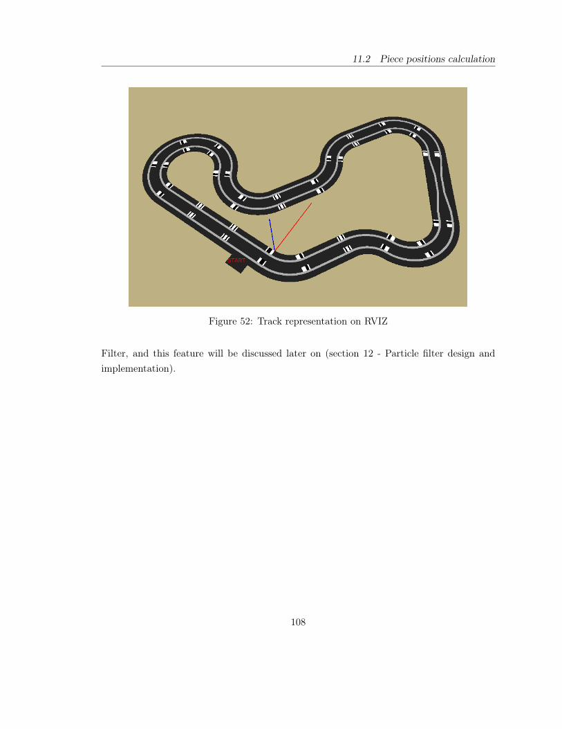
11.2 Piece positions calculation
Figure 52: Track representation on RVIZ
Filter, and this feature will be discussed later on (section 12 - Particle filter design andimplementation).
108

12 Particle filter design and implementation
As it was stated in the introduction, the localization of the car was one of the main goals,so a localization filter was implemented to achieve this requirement, filter which will bedescribed in the following sections. Moreover, in order to evaluate the different filters toimplement, as well as their design, [?] was used as our main reference.
12.1 Localization filter evaluation
As a first step, two different filters were evaluated so as to know which one was more suitablein our project.
First of all, a kalman filter was checked and tested. This filter was designed to use themeasures of the accelerometer and gyroscope in the propagation step and the measuresof the encoder and the magnetometer in the update step, so that theoretically it shouldproduce a good estimation. However, since this filter was unimodal, different tests showedthat the re-localization after a road slip leaded to a wrong localization. Moreover, theaccelerometer and magnetometer had a really high noise. As a consequence, the evaluationof this filter stated that it was not the best option for our project.
As a second option, a particle filter was evaluated. Since this filter was multimodal, itcould reach a better performance after road slips. Furthermore, thanks to the filter motionmodel, which was designed to avoid the use of the accelerometer and the magnetometer,the noise coming from the sensors was not so significant, and therefore, this filter becamea really suitable option for our project. The goal of the next sections will be to explain itsimplementation and design in a deeper level.
12.2 Particle Filter definition
The particle filter, based in a Bayesian model, is a excellent state estimation technique andit is nowadays one of the main methods for robotic localization.
One of its mains advantages is that the state space is not restricted to an specific distribution(as the kalman filter with Gaussian distributions). Moreover, this state space is multimodal,
109

12.2 Particle Filter definition
so that it solves the "Kidnapped robot problem" (case when the robot is moved to aarbitrary localization), problem that we had to faced in our project with the road slips.
The basic idea hidden into the filter algorithm is that it uses a set of particles, representingeach particle an state estimation, so that after each iteration of the filter, the particles withbetter estimation will remain in the set, and the other ones will be eliminated. In order todo that, those particles are weighted proportionally to the accuracy of their estimation, sothat they can be resampled afterwards according to their weight, ending as a consequencewith a set of particles whose particles have state estimation closer to the real state.
Basically, the filter works with the iteration of a series of steps. First of all, the state ofthe particles is propagated from the previous state to the current state , being in robotlocalization this task done using measures of the real system or actuations of the motionmodel. Then, in a second step, the particles are weighted according to other measures,measures which grade the difference between the state of each particle and the real state,being the weight inversely proportionally to this difference, so that the particles whoseestimation is more accurate have a higher weight.
Finally, in a last step, the particles are re-sampled according to their weights, so that theparticles with more accurate estimations are included more times in the set. Therefore,after each iteration, the particles in the set are more and more near to the real state.
In addition to that, it is also often common the introduction of random particles in eachiteration, helping this inclusion to get a better performance. The basic idea is that, ifafter reaching a good estimation, a suddenly change in the state occurs (Kidnapped robotproblem), the new state could no be estimated if this state is far from the old state sinceevery single particle would just be in a wrong state, and therefore all of them would just havea low weight and after the resampling the set would have particles with wrong estimations.However, introducing random particles after the resampling step results in particles inrandom states, and therefore, if a suddenly change happens, some of those particle willeventually be in a state really close to the new state, and thus, they will be re-sampled withhigher probability than the non-random particles, so that the new state will be estimated.By contrast, if there is no change, those random particles would have a low weight andmost of them would disappear in the resampling.
110

12 PARTICLE FILTER DESIGN AND IMPLEMENTATION
12.3 Particle filter design
In order to locate the car 5 variables are required, 3 of them are (x, y, z), and the otherones are the pitch and yaw angles of the car (the roll is not necessary since its value shouldalways be 0 unless a road slip occurs and the car overturns). To a better understanding ofthis issue the figure 53 on page 111 illustrates the representation of this 3 angles.
Figure 53: Yaw, roll and pitch edges representation
Moreover, since the track is a discrete system with an specific and closed geometry, the filtercan work with a more reduced state. Defining the localization state as (length, side), wherelength is the distance along the track between the current position and the beginning of thetrack, and the side can be either L(left) or R(rigth), the 5-variable state (x, y, z, pitch, yaw)is immediately obtained considering this reduced state and the specific geometry of the track(in other words: in a specific point of the track the car position and the angles of the carare given by the track). The figure 54 on page 112 illustrate the definition of length andside on a specific track.
Taking all this into account, the filter was designed so that it uses 2 independent couple ofpropagation-update steps to estimate the state of the car. The first couple of propagation-update steps propagate the length, calculating the (x, y, z) of every particle with the newpropagated stated, weighting the particles afterwards according to the real position of thecar and the position of the particles. In a second couple of propagation-update steps, theangular speed of the particles is propagated and then it is measured in order to weightagain the particles.
111

12.3 Particle filter design
Figure 54: Filter state representation and definition
12.3.1 Number of particles
Is is of note that the filter should work on different kind of tracks, and the minimum numberof particles to estimate optimally the position of the car varies as a function of the numberof pieces in the track: with smaller number of pieces the total state space is also smaller,thus the localization is easier and the number of particles required is lower, by contrast,higher circuits need a larger number of particle to reach a good estimation because the totalstate space is also larger.
As a consequence, the number of particles was implemented directly proportionally to thenumber of pieces, so that the execution of the filter uses always the minimum computationalresources. However, due to the fact that less than 100 particles leads to a wrong behaviorin any circuit and more than 200 particles causes a good estimation in any circuit, 2thresholds were implemented to avoid a wrong estimation or a overuse of resources due tothis dynamically estimation of the number of particles.
112

12 PARTICLE FILTER DESIGN AND IMPLEMENTATION
12.3.2 Position propagation-update step
In order to propagate the length of the particles only the measures of the encoder arerequired. That is because having the angular speed of the car, the calculation of its linearspeed is imminent, and with this linear speed, it is evident that the relative progress of thecar is the speed of the car multiplied by the time interval between two propagation steps.
Then, once the relative progress of the car is obtained, every particle can be directly prop-agated with this relative progress of the car, so that the absolute length of every particlewould be the previous length + this progress. It is of note that, since the encoder measureshave errors, instead of directly add this relative progress to every particle, the result of agaussian distribution with mean progress and deviation progress
5 is added to the length ofevery particle, so that the relative propagation of every particle is different and the filtercan model this bias in the encoder.
Finally, the side of every particle is also propagated if the particle is a Swap or SwitchPiece. However, whereas in the Swap the particle suffers a side change, in the Switch Piecethis change occurs according to a probability1. The completely propagation algorithm isdescribed in the algorithm 1 in the page 114.
With the absolute length and side of every particle and the geometry of the track, thecalculation of the (x, y, z) of every particle is trivial. As a consequence, the update step iscarried on comparing the position of every particle with the position of the different tagsalong the track. So as to do that, every time the car send a tag reading, the filter checksfor every particle if there is a similar tag near the particle, and as a result it weights theparticle as the inverse of the euclidean distance to this similar tag. The figure 55 in thepage 114 shows the change from (lenght, side) to (x, y, z) of one particle, as well as theposition of the particles:
Moreover, it was necessary to avoid weights too huge or too small which could lead to acompletely bad estimation if there is a wrong tag reading and a random particle is generatednear a tag similar to the wrong tag. Therefore, 2 weight thresholds were implemented: aweight maximum of 10 and a minimum of 0.01. Finally, it is remarkable that in order to
1Since the Switch is a mechanic and not automatic change rule by the computer, the side change mightnot occur
113

12.3 Particle filter design
Algorithm 1 Propagation stepfunction Propagation(encoder, Particles, switch, δt.propSteps)
progress = encoder( radseg )× (π ∗ wheel.diameter)× δt.propStepsfor particle ∈ Particles do
particle.length← particle.length+N (progress, progress5 )if particle.piece = Swap then
particle.side← changeSide(particle.side)else if particle.piece = Switch then
if switch.on then99% probability : particle.side← changeSide(particle.side)
else1%probability : particle.side← changeSide(particle.side)
end if
Figure 55: State representation in (x,y,z) and tag positions
114

12 PARTICLE FILTER DESIGN AND IMPLEMENTATION
speed up the execution of the filter, if the particle is in a piece whose tag differs from thetag read, the weight of this particle is directly calculated as the minimum weight. Theequation of the update step for a particle onto a piece similar to the piece where the car islocated can be seen on the algorithm 2 in the page 115.
Algorithm 2 Update-position stepfunction UpdatePosition(Particles, Tags, tagValue)
for particle ∈ Particles doif particle.piece = tagValue then
index← particle.index
particle.Weight← 1√(Tags[index].x− particle.x)2 + (Tags[index].y − particle.y)2
particle.Weight← max(0.01,min(particle.Weight, 10))else
particle.Weight← 0.01end if
end forend function=0
12.3.3 Angular speed propagation-update step
Since the filter receives encoder values periodically, the propagation step for the particles isshared with previous step, and therefore, it is based in the propagation of the length usingthe value of the enconder. Such algorithm is described in 1 in the page 114. However, thereis a great difference in the update step, the difference now is that the absolute length ofevery particle and the geometry of the track are used to calculate the angles of the car 1, sothat, considering the angles of the particle before and after being propagated and using thedifference between those angles in couple with the time interval between propagation steps,it is evident that the expected angular speed of every particle can be easily calculated.
After that, the update step checks the angular speed of the car measured by the gyroscope,so that it can compare it with the expected angular speed of every particle, being inturn weighted each particle proportionally to the inverse of the difference between the two
1In the other step the length and geometry were used to calculate the (x, y, z) of every particle
115

12.3 Particle filter design
angular speeds. The algorithm of this step can be seen in 3 in the page 116, and it waschosen because it showed the best behavior among all the different equations proportionallyinversely to the difference of the angular speeds which were considered.
Algorithm 3 Update - angular speed stepfunction UpdateAngularSpeed(Particles, Gyroscope, δt.updSteps)
for particle ∈ Particles do
particle.AngSpeed←(particle.Angle− particle.LastAngle)
δt.updStepsparticle.LastAngle← particle.Angle
particle.Weight← 0.001
0.001 + abs(particle.AngSpeed−Gyroscope)end for
end function
It can be clearly seen how now, there are no weight thresholds, and that is because sincethe random particles are not generated in this step, there is no risk of a large wrong weightin a random particle.
It is of note that this step has a higher frequency than the propagation-update step thatuses the tag readings. It is fairly evident that whereas a tag value is obtained once per eachpiece on the track, the value of gyroscope can be obtained several times inside the samepiece of the track.
12.3.4 Resampling and Random Particles
Once the particles are weighted, they are resampled according to its weight, so that particleswith higher weight have higher probability of being resampled.
Moreover, the introduction of random particles was implemented. This particles guaranteethat in case of suddenly change of state (slip road) or a completely wrong state estimationdue to a wrong tag reading, there are always random particles which will eventually belocated in the right state, and therefore the correct state will be estimated.
Nevertheless, this random particles are only generated after the resampling in the propagation-update step that involves the tag reading. The main reason for that is that this generation
116

12 PARTICLE FILTER DESIGN AND IMPLEMENTATION
must be implemented with a low periodicity, otherwise the uses of too many random par-ticles can lead to a wrong estimation of the state. Therefore, since the frequency of theresampling in the step that uses the tags is lower than the resampling that uses the gy-roscope, the generation on the random particles in this resampling suites perfectly therequirements of this filter.
Furthermore, since the goal of those random particle is to estimate the correct state, theywere only generated in the positions where a tag with the same value that the tag that hasbeen read is located. As a result, if there is suddenly change of state, the conversion of thefilter is really quick thanks to the fact that the particles are generated on the very definedset of possible car positions.
Similarly, the number of random particles implemented was function of the entropy ofthe circuit. Circuits with higher entropies are circuits with a composition of pieces moredifferent (higher disorder), and therefore the number of random particle required to estimatea new state after a wrong estimation is lower. That is because in circuits with similar pieces,particles in a wrong state have higher possibility of show a great weight 1, so that the filterwould have more troubles to make the filter converse after a suddenly change of state.However, in a circuit with higher difference of pieces, the number particles in the possiblecorrect state are lower, and therefore, the estimation of the localization is faster becausethe filter can converge quicker.
12.3.5 Localization of the car
In order to extract the positions of the car using the set of particles, the statistical modewas used, so that the particle which appears more times in the set is consider as the carposition.
Moreover, this localization has associated a measure of its accuracy. Considering the numberof particles near the particle that was selected as the statistical mode, it is evident thatmore particle nearby means higher accuracy since the larger number of particles pointingto a similar state, the higher the probability of being this state the correct localization ofthe car.
1Any particles in a straight piece will show a good weight if the car is really in a straight piece
117

12.4 Particle filter test and simulation
In order to represent this confidence in RVIZ, an algorithm that changes the transparencyof the car considering this accuracy was implemented, so that lower accuracy shows highertransparencies.
12.4 Particle filter test and simulation
All the design and description of the particle stated in the previous sections are the resultof days of testing and trying different parameter in the filter.
In order to test it, a simulation of the filter was done in RVIZ, so that its behavior could bechecked with the different modifications that were done during the whole process of testing.
118

13 Artificial Intelligence implementation
Since the last goal of the project was implement an algorithm which could learn the op-timum car speeds along a given track, a Reinforcement Learning algorithm based on aMDP (Markov Decision Process) was used. The next sections will analyze the design andimplementation of this algorithm.
13.1 MDP and Reinforcement Learning algorithm
Markov decision processes are a mathematical implementation for modeling decision makingin situations where outcomes are not completely known and under the control of the decisionmaker. Basically, considering a set of spaces forming the state space and a set of availableactions , a MDP can be understood as the process being in a state S in a time step t, andhaving to take an action a in this time step which might make the process reach a newstate S′ in a time step t+ 1 with a probability P , getting as a result an immediate rewardR due to this transition.
Summarizing, it can be said that a MDP is defined by:
1. A set of states s ∈ S.
2. A set of actions a ∈ A.
3. A transition function T (s, a, s′) stating the probability of transition between states.
4. A reward function R(s, a, s′) stating the immediate reward of a transition.
Moreover, the final goal of the MDP is acquiring a policy which indicate the optimum actionto take in a given state, and a utility function, indicating the sum of the future rewards.The MDP defines also the concept of state value V ∗(s) as the expect future utility froma state s and acting optimally, and the q-state value Q∗(s, a) as the expect future utilitytaking the action a in the state s and then acting optimally. The equation 3 and 4 showthis, where γ is a discounted factor to give preference to immediate rewards.
119

13.2 Project implementation
V ∗(s) = maxaQ∗(s, a) (3)
Q∗(s, a) =∑s′
T (s, a, s′) ∗ [R(s, a, s′) + γ ∗ V ∗(s′)] (4)
Considering this model, what the Q-learning algorithm (specific Reinforcement Learningalgorithm) does is explore the world space, learning the different Q∗(s, a, s′) for every state,getting as a consequence the optimum action for every state. So as to do that, the algorithmexplores the different rewards R(s, a, s′) taking all the possible actions for each state, andrecording the value of the rewards obtained.
Then, considering that Qk+∗1(s, a) =
∑s′ T (s, a, s
′) ∗ [R(s, a, s′) + γ ∗maxaQ∗k(s, a)], wherek is accounts for the time step, when the algorithm makes a transition, it records the valueof RewardT otal = R(s, a, s′) + γ ∗max′aQ∗k(′s, a′), and updates the value of the Q-state as:
Q(s, a) = (1− α) ∗Q(s, a) + (α) ∗RewardT otal (5)
Where α is a factor that balance the learning acquired so far with the new learning reached inthe last transition, giving more importance to latest values, since they Q(s, a) will converge,and thus, the last values are more accurate.
Moreover, this algorithm uses different factors for exploring, for instance, actions with lowor negative rewards are not explored after a certain number of checks, likewise, actionsunexplored tend to have higher probabilities of being chosen.
13.2 Project implementation
Considering the definition above, as well as the fact that the slot car has a lot of inertia,we have considered the state of the car on the MDP as a tuple with four values: the actualsort of piece where the car is located, the next two sort of pieces and the speed set in theprevious state. As a consequence, on one hand, the MDP models the influence of the speedin the current state in the next two states, influence that it can be appreciate as an inertial
120

13 ARTIFICIAL INTELLIGENCE IMPLEMENTATION
force, and modeled considering the next two sort of pieces within the state. Moreover, onthe other hand, the MPD also models perfectly the inertia from the previous state with theinclusion of the speed set in the previous state. Thus, the set S of possible states, given acertain circuit with its specific sequence of pieces, might be defined as follows:
S = ((PieceSequence[i], P ieceSequence[j], P ieceSequence[k], P revAction) |
∀ i = j − 1 = k − 2 ≤ NumPieces and ∀PrevAction ∈ LegalActions)
Regarding the set as actions represented by LegalActions, we decided to discretize thePWM actuations with gaps of 10 between a minimum actuation of 130 (actuation forwhich the car never goes out), and a maximum of 255. Moreover, also the actuation of0 was considered since there might be situations where the car requires to set the speedto the minimum value for safety reasons. Consequently, the set of possible actions can bedefined as:
LegalActions = (0, , 130, 150, 170, 190, 210, 230, 255)
Considering this state space and action space, it is immediately evident that the Q-learningalgorithm should now have a Reward function to measure the performance in the statetransition. As a result, we decided to implement the Reward as a directly measure of thesquare inverse of the time required between 2 states. In other words, the less time the slotcar requires to reach the next state, the higher the Reward obtained by this state.
Reward = 1/TransitionT ime2 (6)
Moreover, we implemented a penalty for slip roads, so that when the car takes more than2 seconds to reach the next state, the MDP assumes that the car went out of the track orthat it stopped in the middle of a piece, and it gives a penalty to this Q-state of -500, valuefive times higher that the highest positive Rewards between states, which guarantee that ifthe car suffers a couple of slip roads in a certain Q-state, then this Q-state would acquiresuch a negative value that even some good performances will not give a positive value to
121

13.3 New Q-States Exploration
this Q-state. This decision was made considering that the car must drive trying to avoidany kind of slip road risk, driving safety in a giving track.
Furthermore, the MPD also evaluates the possibility of realizing a switch side when itreaches a Switch piece. Basically, when it reaches a Switch, it checks for every next pieceuntil the next Switch, the maximum Q-value among the possible states for every piece. Asa result, it switches if the result of this evaluation states that the Q-values of the statesafter switching are higher than without switching, because that means that the Rewardobtained in those states are expected to be bigger, thus, the time required to cross all thosepieces smaller.
Finally, it is also of note that the MDP receives the current position of the car from theParticle Filter, which sends the index of the piece where the car is located. As a result,if the Particle Filter sends two piece indexes which they are not consecutive, the MDPassumes that the Particle Filter might be lost, stopping the training and setting the speedat 130 until two consecutive index are received1.
13.3 New Q-States Exploration
In order to find out the optimum action given an state, using the conventional model theMDP would just check the optimum Q-state for this state, and the optimum action wouldbe the the action that this Q-state associated.
However, since our model has a really great inertia, we contemplated that not only theQ-states associated with the state under evaluation should be be considered, but also the Q-states in the next state that we might find if we choose the action a ∈ LegalActions shouldbe evaluated. Therefore, the optimum action was selected as the action that maximize thesum of (Q−state+max(Q−statesnext). The algorithm 4 in the page 123 illustrates betterthis process.
Considering this optimum action, that higher speed means better rewards and that the car is
1Since the car has a discrete number of pieces, the pieces might be enumerated according to its order inthe track, being the START piece the number 0, therefore, two index not-consecutive might mean that theParticle Filter got lost
122

13 ARTIFICIAL INTELLIGENCE IMPLEMENTATION
Algorithm 4 Optimum action selectionfunction Optimum Action(LegalActions, State)
Maximum = 0optimumAction = 0for action ∈ LegalActions do
next_State← getState(prevState = State, prevAction = action)Q_max← Q− state(State, action) +max(Q− states(state = next_State))if Maximum < Q_max then:
optimumAction = actionMaximum = Q_max
end ifend forreturn optimumAction
still training1, the next speed action ∈ LegalActions might produce a higher Reward, thus,the MDP chooses with 40% probability the optimum Q-state and with a 40% probabilitythe Q-state involving the next action inside LegalActions.
As a result, the slot-car will try higher speeds until the Reward is negative, when, at thatpoint, the MDP will choose with 45% probability the optimum Q-state which will performthe higher Reward, and with 45% probabilities the first Q-state with negative reward, andit will oscillate in this threshold, updating those two Q-states.
Finally, a 10% probability was implemented to choose random Q-states. Those randomstates leaded to a faster learning since higher speed were tested before, and therefore, theoptimum Q-states could be tested before than if the MDP just were trying incremental-speed Q-states.
It is important to remark that, despite to the fact that the model stated above was the modelimplemented to generate the optimum training, during the first days we first implementedthe same model but with a 80% probability of random states rather than the 10% probabilitystated above. That selection was made for the same reason stated for the 10% probabilitychoice: doing that, higher speeds were tested before, and consequently, the convergence tothe optimum Q-state was reached earlier.
1Because the car is still training, the optimum Q-state could not be the optimum, instead some higherspeeds might belong to that optimum
123

13.4 MDP testing
13.4 MDP testing
In order to check that the MDP was really learning, a small script in Octave was imple-mented so as to represent the different Q-values. Using them, the MDP can be betterundersood.
For instance, the figure 56a on page 125 shows the Q-values of the State StraightStraightStraightwhere the previous action is plotted against the current action. It can be seen how the gen-eral patter is no matter the previous speed, the best Q value are normally the highestactions since when it has three straight in front of it, the best action is accelerate.
By contrast, the figure 56b show the same but for the case of StraightStraightCurveRight,and from it, it can be seen how now, since it must face a curve soon, higher speeds arenot always the best choices, specially when the previous speed are also high. Likewise, thefigure 56c illustrates StraightCurveRightCurveRight, as it is evident, now most of casesare penalized since in the curve, the car used to crash due to high previous speeds and theirinertia. As a result, this case shows how the optimum cases occurs when the previous speedis 0 and the car is being moved by the inertia, and then, the MDP sets it to 130, makingthe curve driving smother.
13.5 Learning extrapolation
Thanks to the fact that our model uses as state the sort of pieces and the previous speeds,the state space is limited, therefore, once the MDP has been trained for every state, thislearning can be used in any Carrera circuit as long as the pieces used in this circuit shareshape and geometry with the pieces used in this project.
This consideration was the main difference with previous implementations, which consideredoptimum speeds for an specific circuit, rather than a self-learing model which once it haslearnt it can be used for any track.
124

13 ARTIFICIAL INTELLIGENCE IMPLEMENTATION
(a) State Straight Straight Straight
(b) State Straight Straight Curve Right
(c) State Straight Curve Right Curve Right
Figure 56: MDP states simulation125

14 ROS nodes interconnection
Considering the communication implemented in ROS and stated in the previous sections,it is really helpful to obtain a general picture of all ROS nodes implemented, as well astheir topics, either the ones where they publish and the other ones which are subscribedto. The figure 57 on page 126 illustrate this communication, being each ellipse nodes andthe rectangles topics, reflecting the arrows the relation between node and topic (publisheror subscriber).
Figure 57: ROS nodes communication
It can be seen the implementation of 5 ROS nodes, which execute different functions.
1. /ParticleFilter implements the Particle Filter stated before, publishing in the topics/Car and /Particles which RVIZ is subscribed to represent the car and the particlespositions. Furthermore, it also publishes in /MDPPosition in order to indicate theMDP the position of the car within the track. In addition, it is subscribed to /track-Coordinates, so that it can know the boundaries of the pieces of the track, which isrequired in order to calculate the Weight of the particles. Finally, it is also subscribedto /SensorSerialReceive to acquire the value of the encoder, gyroscope and tags, and
126
14 ROS NODES INTERCONNECTION
to /SwitchOnOff so that it can know the probabilities of a switch in the next switchpiece.
2. /SerialCom receives every single package for the car, checking that the package itscorrect, and publishing it in the specific topic. Therefore, it publishes in /SensorSe-rialReceive the specific sensor values required for the Particle Filter. Likewise, itpublishes in /SystemSerialReceive the system status values and in /TrackSerialRe-ceive the track sequence when a new track is detected in the EXPLORING mode ofthe slot-car. On the other hand, it is subscribed to /SwitchOnOff to detect the Switchstate and send the correspondent signal to the specific port that rules the switch, andit is subscribed as well to /SerialSend, which is the topic where other topics write thedifferent orders to be sent to the car.
3. /TrackNode is subscribed to /TrackSerialReceive, so that when a new track sequenceis recognized by the car and sent, this node creates a Markers for each piece of thetrack and their positions, using the sequence received as base for this function. Then,it publishes the Markers in /Track, which is an specific RVIZ topic for Markers,representing then the track in RVIZ. Moreover, it also publishes in /trackCoordinatesthe origin coordinates of the different pieces of the track, those coordinates can actas boundaries so as to calculating the Weights in the Particle Filter.
4. /Interface is the node that manages a GUI for direct communications with the user.It publishes in /SerialSend because among the main functions of the GUI are directcommand to the car, commands as set the status or mode, or even the car speedwhen the car is in the Slave mode. Moreover, it also publishes in /SwitchOnOff sincethe user might have the opportunity to activate a switch track in the specific piece.Finally, it is subscribed to /SystemSerialReceive since it need the data of the car toshow it to the user.
5. /CarControl manages the execution of the MDP. It is evident that this node hasto publish in /SerialSend in order to send the speed command to the car, and in/SwitchOnOff so that it can evaluate between doing or not a switch track accord-ing to the succession of the optimum states between two consecutive track switches.Moreover, it is subscribed to /MDPTraining, topic which indicates if the MDP istraining, or by contrast selecting all the time the optimum action in each state.
127

15 Main drawbacks of our model
The model we have described and using during this project had some drawbacks in spite ofbeing successfully implemented. Those drawbacks made us work over and over again overthem, trying to overcome them, some times with failed results. The goal of this section islist them, and explain why those problems were that decisive:
1. Dirty on the track: since the track was located in the floor and in the middle ofa environment with more activities than just the track and the slot-car, the tendencyof the track was to acquire dust all over it. As a result, the wheel of the car used toget this dust and dirtied the tags of the pieces, so that after one week of use the carstarted to have troubles to read the tags, since most of them were full of dirt. In orderto solve this problem, we had to change the tags of the track regularly and we had toclean the track even more often. Moreover, the dust of the track not only dirtied thetags, but it also destabilized the slot-car in the curves since the grip of the car waslower due to this dust.
2. Illumination: another problem we had to face was related with the illumination.Since the tags were read with an optic sensor, the sensitivity of the sensor to theillumination conditions was really high, and sometimes we had troubles when wechange the environment. Thus, we end up locating the track in the same spot andwith the lights of the room always on.
3. Weight: since the car had mounted on the surface the whole sensorial system, theweight doubled. As a consequence, the car suffer three main problems:
(a) The car had to make bigger efforts to accelerate and decelerate, resulting in ahigher power supply to the motor. This increment on the power supply leaded toa really high temperature conditions on the motor, which in turn made impossiblethe continuous use of the car for training purpose since the high temperaturecould damage the motor and the hardware.
(b) Due to the high weight, the inertia of the car was really bigger, and as we alreadystated in the previous sections, that result in a MDP state which had to considerprevious speeds and following pieces in order to model this huge inertia.
128

15 MAIN DRAWBACKS OF OUR MODEL
(c) The third and last problem due to the weight was that, since now the chassis hadto hold a double weight, some parts of the chassis could not resist it and theybroke. For instance, the small flap that guided the car through the guideway wasbroken several times because it could not turn properly the slot car in the curves.Likewise, the wheels of the car were separated from their edges few times, havingto stick them over and over again to this edge.
129
16 Conclusion and summary
After implementing everything that has been specified so far, it can be concluded that theproject has been finished.
The slot-car has now a completely and reliable sensor system and a wireless communicationwith a computer, which makes possible the also implemented Particle Filter, which in turndevelops a complete localization of the vehicle. Moreover, with its integrated self-learningspeed algorithm, algorithm that makes the car race by itself, the car can set automaticallyoptimum speed along the track.
130

17 Flow diagrams
17.1 Low level
17.1.1 Main.c
Main
Initialization
EEPROM writing
Control System Status
Time base
Initialization
Serial, EEPROM Motor Init
Get data EEPROM
Restart car last status
Sensors initialization
Stop
Reset Watchdog
Init watchdog
PID init
Initialization Vector
Set system status and mode
Set LED frequency
Set periods for Sensor, IMU,
system and PID reports
Stop
131
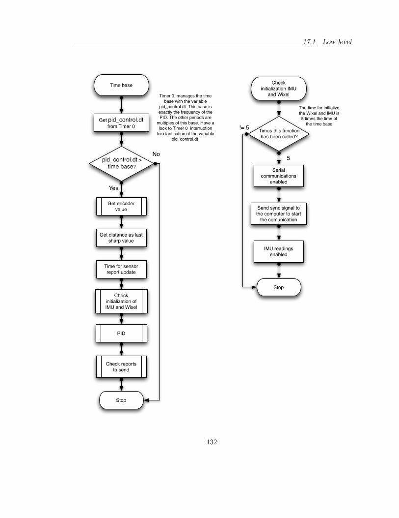
17.1 Low level
Time base
Timer 0 manages the time base with the variable
pid_control.dt. This base is exactly the frequency of the PID. The other periods are
multiples of this base. Have a look to Timer 0 interruption
for clarification of the variable pid_control.dt
pid_control.dt > time base?
Check initialization of IMU and Wixel
Check reports to send
Stop
No
Yes
Get pid_control.dt from Timer 0
Check initialization IMU
and Wixel
Times this function has been called?
The time for initialize the Wixel and IMU is 5 times the time of
the time base
Serial communications
enabled
Send sync signal to the computer to start
the comunication
IMU readings enabled
5
Stop
!= 5
PID
Time for sensor report update
Get distance as last sharp value
Get encoder value
132

17 FLOW DIAGRAMS
Check reports to send
Serial Channel initialized?
Sensor report enabled?
Function calls multiple of
sensor period?
IMU report enabled?
Function calls multiple of IMU
period?
System report enabled?
Function calls multiple of system
period?
PID report enabled?
Function calls multiple of PID
period?
Stop
Sensor | IMU | System | PID report periods are multiples of the time base period, and check
reports is executed with frequency time base, thus, counting the number of times this function is executed,
all those periods can be controlled as divisors of the number of calls,
Yes
No
Yes
Yes
No
No
No
No
Yes
No
Yes
No
Yes
Yes
Yes
Yes
No
No
Send sensor report
Send system report
Send PID report
Send IMU report
Update encoder value for sensor
report
133

17.1 Low level
Send sensor report
New tag value?
Send Package
No
Yes
Send IMU report
Send Package
Stop
Stop
Send system report
Send Package
StopNew tag value
OFF
Package = 'r' Package = 'u' Package = 's'
Package += gyroscope(x,y,z) +
accelerometer(x,y,z) + magnetomer(x,y,z)
Package += gyroscope
Package += encoder + dt
encoder
Package += gyroscope
Package += tag value + time between tags
Package += system mode
Package += system status
Package += motor actuation
The times 0 in its interruption
manages time between tags as well as it did with
pid_control.dt
134
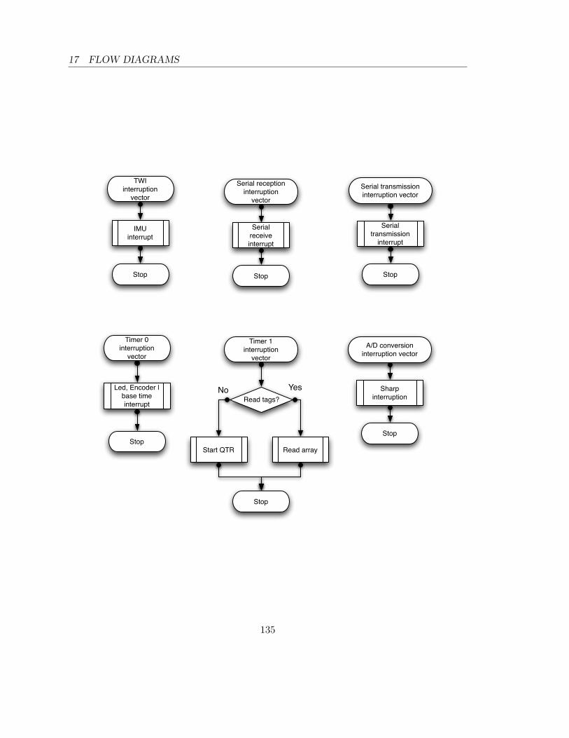
17 FLOW DIAGRAMS
TWI interruption
vector
IMU interrupt
Stop
Serial reception interruption
vector
Serial receive interrupt
Stop
Serial transmission interruption vector
Serial transmission
interrupt
Stop
Timer 0 interruption
vector
Led, Encoder | base time interrupt
Stop
Timer 1 interruption
vector
Read array
Stop
A/D conversion interruption vector
Sharp interruption
Stop
Read tags?
Start QTR
YesNo
135

17.1 Low level
17.1.2 Array.c
Start QTR
Keep reading?
Set QTR ports as inputs to read
Timer 1 initialization to
measure capacitor discharging threshold
Timer 1 complete desactivation
Stop
No
Yes
Read array
Read QTR ports
Set QTR ports as outputs to capacitor
charging
Timer 1 initialization to
capacitor charging
Stop
Tag calculation
136

17 FLOW DIAGRAMS
Tag calculation
Is burst-reading on?
Is tag value a valid value?
Storage tag value inside tag array
Is tag value BLACK?
Is tag value a valid value?
Storage tag value inside tag array
Calculation the current tag as the mode whithin the
tag-burst
Burst-reading ON
Burst-reading ON
New tag value ON
Update time between tag
readings
System control
Stop
137

17.1 Low level
17.1.3 Status_control.c
Control system status
Status has changed?
New Status Value?
Set car speed to 0
Set car speed to exploring
speed
OFF RUNNING
EXPLORING |GO TO STARTCHECKING MAP
Stop
System Mode = AUTONOMOUS?
Check map
Set car speed to 0
Yes
No
138

17 FLOW DIAGRAMS
Check map
Get map from EEPROM
Check map consistency
Is map consistent?
Set status to EXPLORING
Set status to OFF
Stop
No Yes
Send map report
139
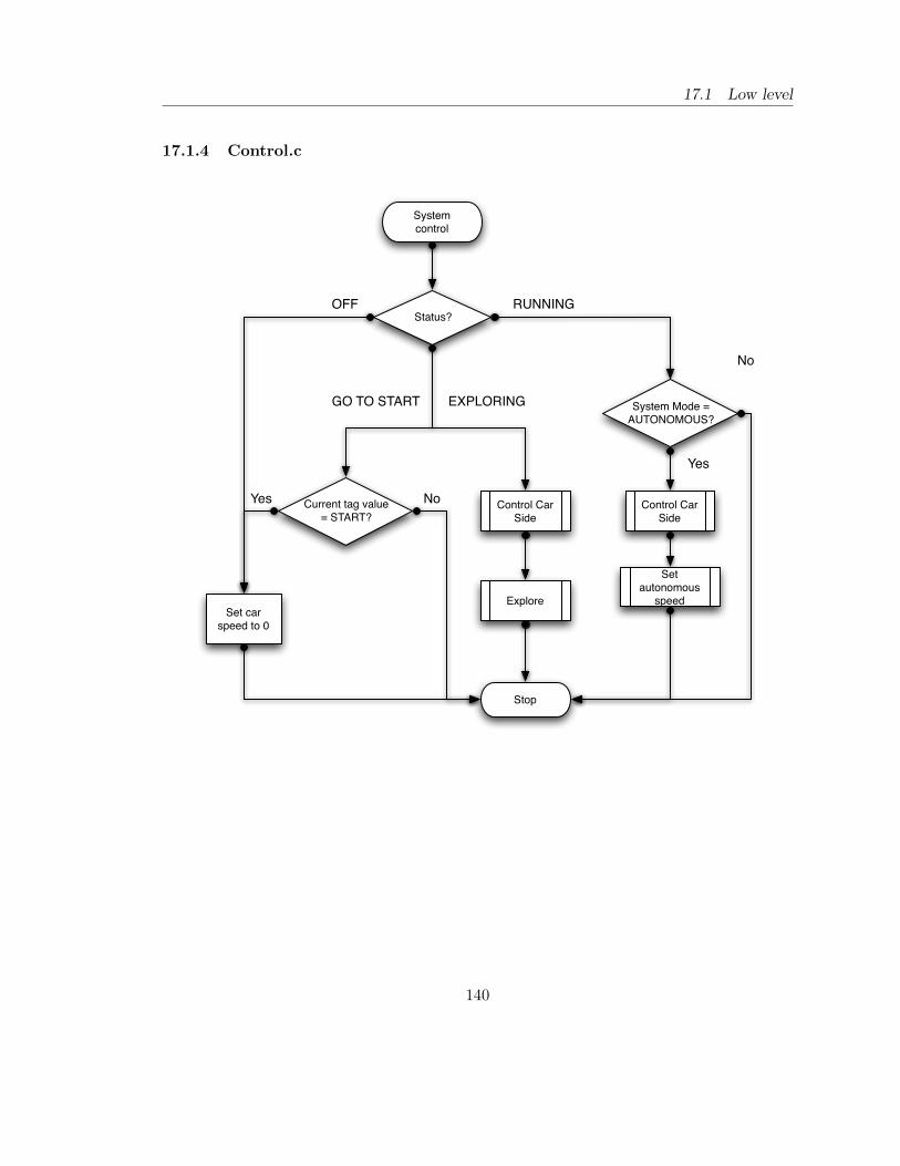
17.1 Low level
17.1.4 Control.c
System control
Status?
Set car speed to 0
OFF RUNNING
EXPLORINGGO TO START
Stop
System Mode = AUTONOMOUS?
Yes
No
Control Car Side
Explore
Set autonomous
speed
Control Car Side
Current tag value = START?
Yes No
140
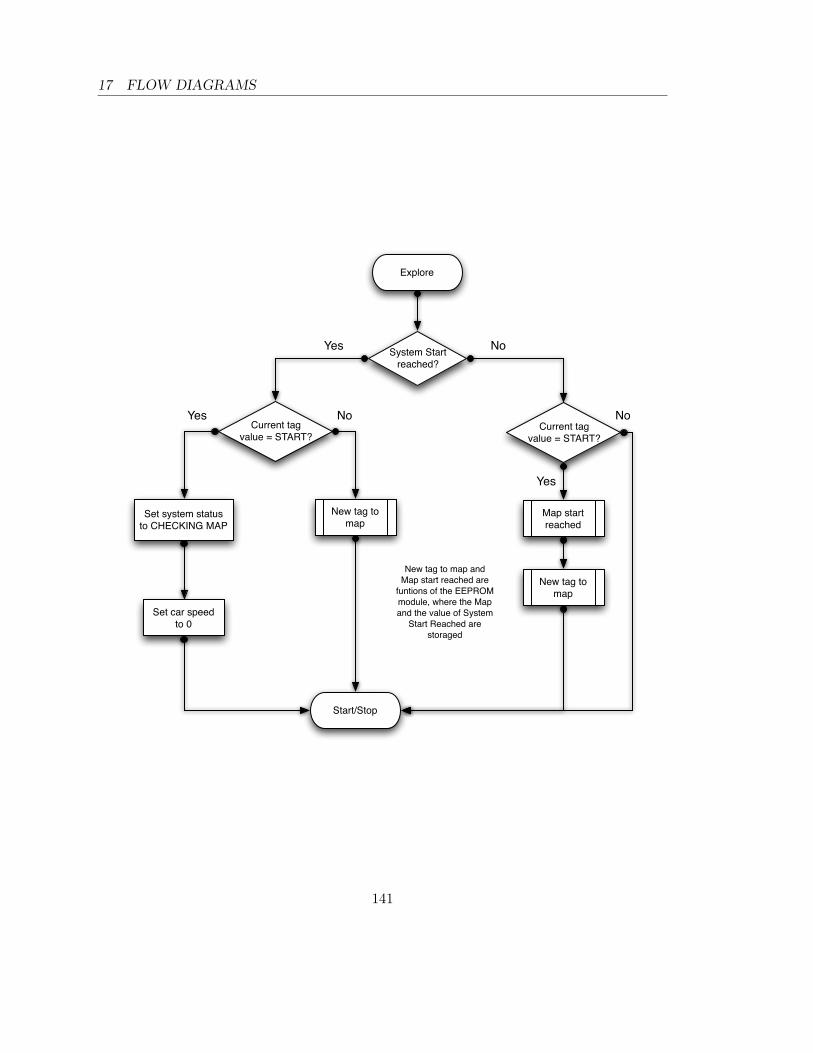
17 FLOW DIAGRAMS
Explore
System Start reached?
Current tag value = START?
Map start reached
New tag to map
Current tag value = START?
New tag to map
Set system status to CHECKING MAP
Set car speed to 0
New tag to map and Map start reached are
funtions of the EEPROM module, where the Map and the value of System
Start Reached are storaged
Start/Stop
Yes No
Yes
Yes
NoNo
141
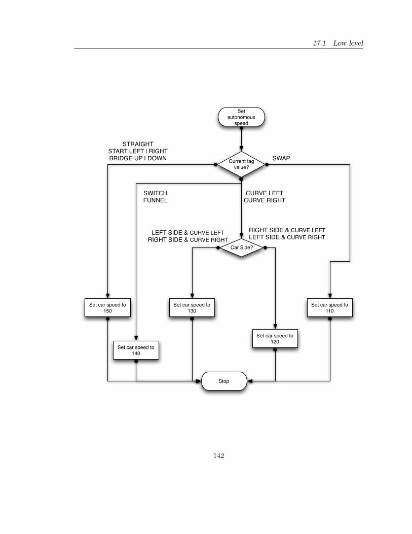
17.1 Low level
Set autonomous
speed
Current tag value?
Set car speed to 150
Set car speed to 130
Set car speed to 120
Car Side?
Set car speed to 140
Set car speed to 110
STRAIGHTSTART LEFT | RIGHTBRIDGE UP | DOWN
CURVE LEFTCURVE RIGHT
SWITCHFUNNEL
LEFT SIDE & CURVE LEFTRIGHT SIDE & CURVE RIGHT
RIGHT SIDE & CURVE LEFTLEFT SIDE & CURVE RIGHT
SWAP
Stop
142

17 FLOW DIAGRAMS
Control Car Side
Current tag value?
Car side = left side
Car side = right sideCurrently side?
Car side = left side
Car side = right side
Stop
START LEFT START RIGHT
SWAP
LEFT SIDERIGHT SIDE
143

17.1 Low level
17.1.5 Eeprom.c
EEPROM writing
Get next (address,data) from
EEPROM buffer
EEPROM data writing
EEPROM buffer empty?
No
Yes
Reading buffer Index = writing buffer index?
Stop
Yes
No
Inc. reading buffer index
EEPROM buffer is not full
EEPROM buffer is empty
Buffer writing
EEPROM buffer full?
Storage in buffer (address, data)
Writing buffer Index = reading
buffer index?
Stop
Yes
No
Inc. writing buffer index
EEPROM buffer is not empty
EEPROM buffer is full
No
Yes
144

17 FLOW DIAGRAMS
Set LED slot
LED slot has changed?
Buffer writing (LED slot address,
LED slot )
Update LED slot
Stop
No
Yes
Set map length
map length has changed?
Buffer writing (Map length
address, map length )
Stop
No
Yes
Set Map Start Reached
Map Start Reached = True
Buffer writing (Start Reached address, Map
Start Reached)
Stop
Map Start Reached has
changed?
No
Yes
New tag to map
Buffer writing (Start Map address + map length, Tag
Value )
Stop
Inc. length map
Set map length
145

17.1 Low level
Set Motor Speed
Update Motor Speed
Buffer writing (Speed address, Motor Speed )
Stop
Set System Status
System Status has changed?
Update System Status
Buffer writing (System status
address, System Status)
Stop
No
Yes
Set System Mode
System Mode has changed?
Update System Mode
Buffer writing (System mode
address, System Mode)
Stop
No
Yes
Set Car Side
Car Side has changed?
Update Car Side
Buffer writing (Car side
address, Car Side)
Stop
No
Yes
146

17 FLOW DIAGRAMS
Set sensor report
Set sensor report period
Sensor report enable has changed?
Sensor report period has changed?
Buffer writing (sensor report
address, sensor report enable )
Update sensor report enable
Stop
Update sensor report period
Buffer writing (sensor period
address, sensor report period )
Stop
No
Yes
No
Yes
Set system report
System report enable has changed?
Buffer writing (system report
address, system report enable )
Update system report enable
Stop
No
Yes
Set system report period
System report period has changed?
Update system report period
Buffer writing (system period
address, system report period )
Stop
No
Yes
147
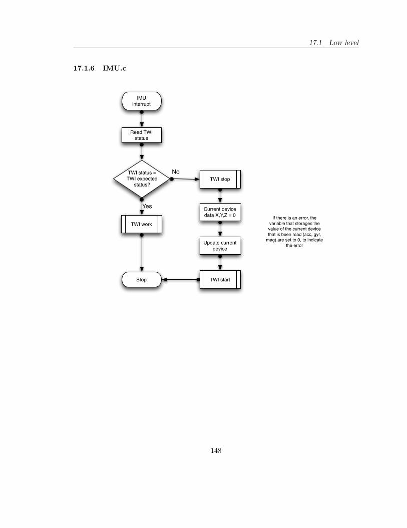
17.1 Low level
17.1.6 IMU.c
IMU interrupt
Read TWI status
TWI status = TWI expected
status?
TWI work
TWI stop
Current device data X,Y,Z = 0 If there is an error, the
variable that storages the value of the current device that is been read (acc, gyr,
mag) are set to 0, to indicate the errorUpdate current
device
TWI startStop
Yes
No
148
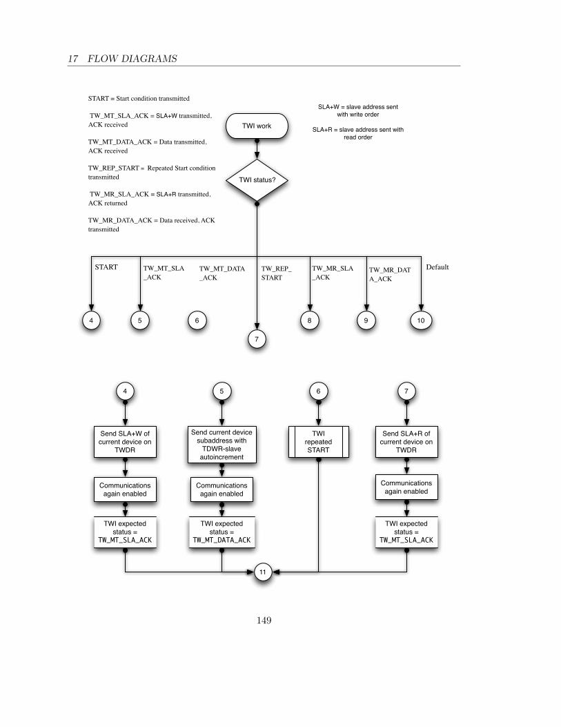
17 FLOW DIAGRAMS
TWI work
TWI status?
4 5 6
7
8 9 10
START TW_MT_DATA_ACK
TW_REP_START
TW_MR_SLA_ACK
TW_MR_DATA_ACK
Default
SLA+W = slave address sent with write order
SLA+R = slave address sent with read order
4
Send SLA+W of current device on
TWDR
TWI expected status =
TW_MT_SLA_ACK
START = Start condition transmitted
TW_MT_SLA_ACK = SLA+W transmitted, ACK received
TW_MT_DATA_ACK = Data transmitted, ACK received
TW_REP_START = Repeated Start condition transmitted
TW_MR_SLA_ACK = SLA+R transmitted, ACK returned
TW_MR_DATA_ACK = Data received, ACK transmitted
TW_MT_SLA_ACK
5
Send current device subaddress with
TDWR-slave autoincrement
TWI expected status =
TW_MT_DATA_ACK
6
TWI repeated START
7
Send SLA+R of current device on
TWDR
TWI expected status =
TW_MT_SLA_ACK
11
Communications again enabled
Communications again enabled
Communications again enabled
149

17.1 Low level
TWI start
Send START in the SDA line
TWI expected status = START
Stop
TWI stop
Send STOP in the SDA line
Stop
STOP executed and bus released?
TWI repeated START
TWI expected status =
REPEATED START
Stop
TWI start
No
Yes
8
Read and store data from device
6 bytes of current devices
has been read?
TWI expected status =
TW_MT_SLA_ACK
Communications again enabled
TWI expected status =
TW_MR_SLA_NACK
Communications again enabled
9
TWI stop
Set next device to read as
current device
TWI start
10
Set error
Stop
YesNo
11
150

17 FLOW DIAGRAMS
17.1.7 Motor.c
Led, Encoder | base time interrupt
Timer 0 interruption is initialized with the period
required according to the slot that the LED is
usingpid_control.dt += Timer 0 period +
Timer 0 current value
time between tags += Timer 0 period +
Timer 0 current value
Restart TImer 0 with the period required
for the LED
Hall sensor port value has changed?
Invert value of LED port
Stop
NoIncrement
encoder_value
Yes
Get encoder value
Return encoder_value and reset this
variable
Stop
151

17.1 Low level
17.1.8 PID.c
PID
Reference = 0 ?
Distance < MIN distance?
Set speed to 0Convert reference
in PWM to reference in number
of ticks
PID calculation
Stop
Yes
Yes
No
No
Set speed to PID speed
152

17 FLOW DIAGRAMS
PID calculation
Error = reference - encoder
Integral_error += Error *dt
PID speed = KP*Error +
KI*Integral_error
Stop
Send system report
Send Package
Stop
Package = 'p'
Package += PID actuation in ticks
Package += PID error
Package += PID actuation in PWM
Package += PID integral part
Package += PID proportional part
153

17.1 Low level
17.1.9 Sharp.c
Sharp interruption
Sharp value = AD converter
value
Start a new conversion
Stop
Sharp get data
Package = h + Sharp value
Send package
Stop
154

17 FLOW DIAGRAMS
17.1.10 Serial.c
Serial receive interrupt
START byte, STOP byte or
Serial receiving?
START?
STOP?
Buffer_package empty?
Allocate buffer_package
Fail?
Serial is not receiving
Send NAK
Reallocate buffer_package
Storage data in buffer
Serial is receiving
Read new package
Serial is not receiving
Release buffer memory
Stop
No
No
No
No
No
Yes
Yes
Yes
Yes
0
0
155

17.1 Low level
Read new package
Get next byte from raw package
CONTROL byte?
Next byte is masked
Byte is masked? Unmask byte
Storage byte
Last byte of the raw
package?
CRC matches?
Package interpretation
Send ACK
Send NAK
Stop
Update CRC
Yes
Yes
Yes
Yes No
No
No
No
156

17 FLOW DIAGRAMS
Package interpretation
ORDER = first byte within package
ORDER?
Set system status Set motor
speed
Initialization vector
Send PID report
Send sensor report
Send system report
Send IMU report
Send motor value
S M m r
I u s p
Stop
157

17.1 Low level
Send new package
Buffer transmission full or Serial
Channel not init.?
Allocate space for the new package Fail?
Insert START byte in buffer
Get next byte to buffer
CONTROL byte?
Yes
No
Insert CONTROL byte in buffer
Mask next byte Insert next byte in buffer
Last byte?
Calculate CRC and buffer_space considering
control bytes
1
2
2
No
Yes
Yes
No
No
Yes
158

17 FLOW DIAGRAMS
Insert CRC byte in buffer
Writing buffer Index = reading
buffer index?
Yes
Inc. writing buffer index
Buffer transmission is
full
1
CRC value CONTROL
byte?Mask CRC
Insert STOP byte in buffer
Serial is transmitting?
Serial is transmitting
Send first byte package within
buffer
Stop2
Yes
No
Insert CONTROL byte
in buffer
No
Init. reading package index
No
Yes
159

17.1 Low level
Serial transmission
interrupt
Currently sending
package?
Send next byte buffer within
package
Inc. reading package index
Response has been
sent?Response not
sent
Buffer is not full
Release package memory space
within buffer
Buffer transmission
empty?
Yes
Inc reading buffer index
Response to be sent?
Send response
Response has been sent
Send first byte next package within buffer
Init. reading package index
Serial is not transmitting
Stop
3
3
No
Yes
No
Yes
No
Yes
No
160

17 FLOW DIAGRAMS
Serial response
Serial init.?
Serial transmitting
Response to be sent
Send response
Response has been sent
Yes
Serial is transmitting Stop
Yes
No
No
Send ACK
Serial response
(ACK)
Stop
Send NAK
Serial response
(NAK)
Stop
Send SYN
Serial response
(SYN)
Stop
161

17.1 Low level
17.1.11 Track.c
Check map consistency
Calculation of (Ax,Ay) of the piece
For each piece in map
Update (x,y)map as (x,y)map + (Ax,Ay)
Create error code according to (x,y)
(x,y)map = initial (x,y)map
Stop
Send map report
New system map?
Create map package = system map + error
code
Send package (map package)
StopYesNo
(Ay, Ay) = differencebetween beginning
and ending of the piece
Error code = 0 (no error)
162

17 FLOW DIAGRAMS
17.2 High level
17.2.1 Track node
163

17.2 High level
17.2.2 Particle Filter node
164

17 FLOW DIAGRAMS
17.2.3 MDP node
165

17.2 High level
166

17 FLOW DIAGRAMS
167