Feature matching

Digital Visual Effects, Spring 2005Yung-Yu Chuang2005/3/16

with slides by Trevor Darrell Cordelia Schmid, David Lowe, Darya Frolova, Denis Simakov, Robert Collins and Jiwon Kim

Announcements

• Project #1 is online, you have to write a program, not just using available software.

• Send me the members of your team.• Sign up for scribe at the forum.

Blender

http://www.blender3d.com/cms/Home.2.0.htmlBlender could be used for your project #3 matchmove.

In the forum

• Barycentric coordinate• RBF

Outline

• Block matching• Features• Harris corner detector• SIFT• SIFT extensions• Applications

Correspondence by block matching

• Points are individually ambiguous• More unique matches are possible with small

regions of images

Correspondence by block matching Sum of squared distance

Image blocks as a vector Image blocks as a vector

Matching metrics Features

• Properties of features• Detector: locates feature• Descriptor and matching metrics: describes and

matches features

• In the example for block matching:– Detector: none– Descriptor: block– Matching: distance

Desired properties for features

• Invariant: invariant to scale, rotation, affine, illumination and noise for robust matching across a substantial range of affine distortion, viewpoint change and so on.

• Distinctive: a single feature can be correctly matched with high probability Harris corner detector

Moravec corner detector (1980)

• We should easily recognize the point by looking through a small window

• Shifting a window in any direction should give a large change in intensity

Moravec corner detector

flat

Moravec corner detector

flat

Moravec corner detector

flat edge

Moravec corner detector

flat edgecorner

isolated point

Moravec corner detector

Change of intensity for the shift [u,v]:

[ ]2

,( , ) ( , ) ( , ) ( , )

x yE u v w x y I x u y v I x y= + + −∑

IntensityShifted intensity

Window function

Four shifts: (u,v) = (1,0), (1,1), (0,1), (-1, 1)Look for local maxima in min{E}

Problems of Moravec detector

• Noisy response due to a binary window function• Only a set of shifts at every 45 degree is

considered• Responds too strong for edges because only

minimum of E is taken into account

Harris corner detector (1988) solves these problems.

Harris corner detector

Noisy response due to a binary window functionUse a Gaussian function

Harris corner detector

Only a set of shifts at every 45 degree is consideredConsider all small shifts by Taylor’s expansion

∑

∑

∑

=

=

=

++=

yxyx

yxy

yxx

yxIyxIyxwC

yxIyxwB

yxIyxwABvCuvAuvuE

,

,

2

,

2

22

),(),(),(

),(),(

),(),(2),(

Harris corner detector

[ ]( , ) ,u

E u v u v Mv⎡ ⎤

≅ ⎢ ⎥⎣ ⎦

Equivalently, for small shifts [u,v] we have a bilinearapproximation:

2

2,

( , ) x x y

x y x y y

I I IM w x y

I I I⎡ ⎤

= ⎢ ⎥⎢ ⎥⎣ ⎦

∑

, where M is a 2×2 matrix computed from image derivatives:

Harris corner detector

Responds too strong for edges because only minimum of E is taken into account

A new corner measurement

Harris corner detector

[ ]( , ) ,u

E u v u v Mv⎡ ⎤

≅ ⎢ ⎥⎣ ⎦

Intensity change in shifting window: eigenvalue analysis

λ1, λ2 – eigenvalues of M

direction of the slowest change

direction of the fastest change

(λmax)-1/2

(λmin)-1/2

Ellipse E(u,v) = const

Harris corner detector

λ1

λ2

Cornerλ1 and λ2 are large,λ1 ~ λ2;E increases in all directions

λ1 and λ2 are small;E is almost constant in all directions

edge λ1 >> λ2

edge λ2 >> λ1

flat

Classification of image points using eigenvalues of M:

Harris corner detector

Measure of corner response:

( )2det traceR M k M= −

1 2

1 2

dettrace

MM

λ λλ λ

== +

(k – empirical constant, k = 0.04-0.06)

Another view Another view

Another view Summary of Harris detector

Harris corner detector (input) Corner response R

Threshold on R Local maximum of R

Harris corner detector Harris Detector: Summary

• Average intensity change in direction [u,v] can be expressed as a bilinear form:

• Describe a point in terms of eigenvalues of M:measure of corner response

• A good (corner) point should have a large intensity change in all directions, i.e. R should be large positive

[ ]( , ) ,u

E u v u v Mv⎡ ⎤

≅ ⎢ ⎥⎣ ⎦

( )21 2 1 2R kλ λ λ λ= − +

Harris Detector: Some Properties• Partial invariance to affine intensity change

Only derivatives are used => invariance to intensity shift I → I + b

Intensity scale: I → a I

R

x (image coordinate)

threshold

R

x (image coordinate)

Harris Detector: Some Properties

• Rotation invariance

Ellipse rotates but its shape (i.e. eigenvalues) remains the same

Corner response R is invariant to image rotation

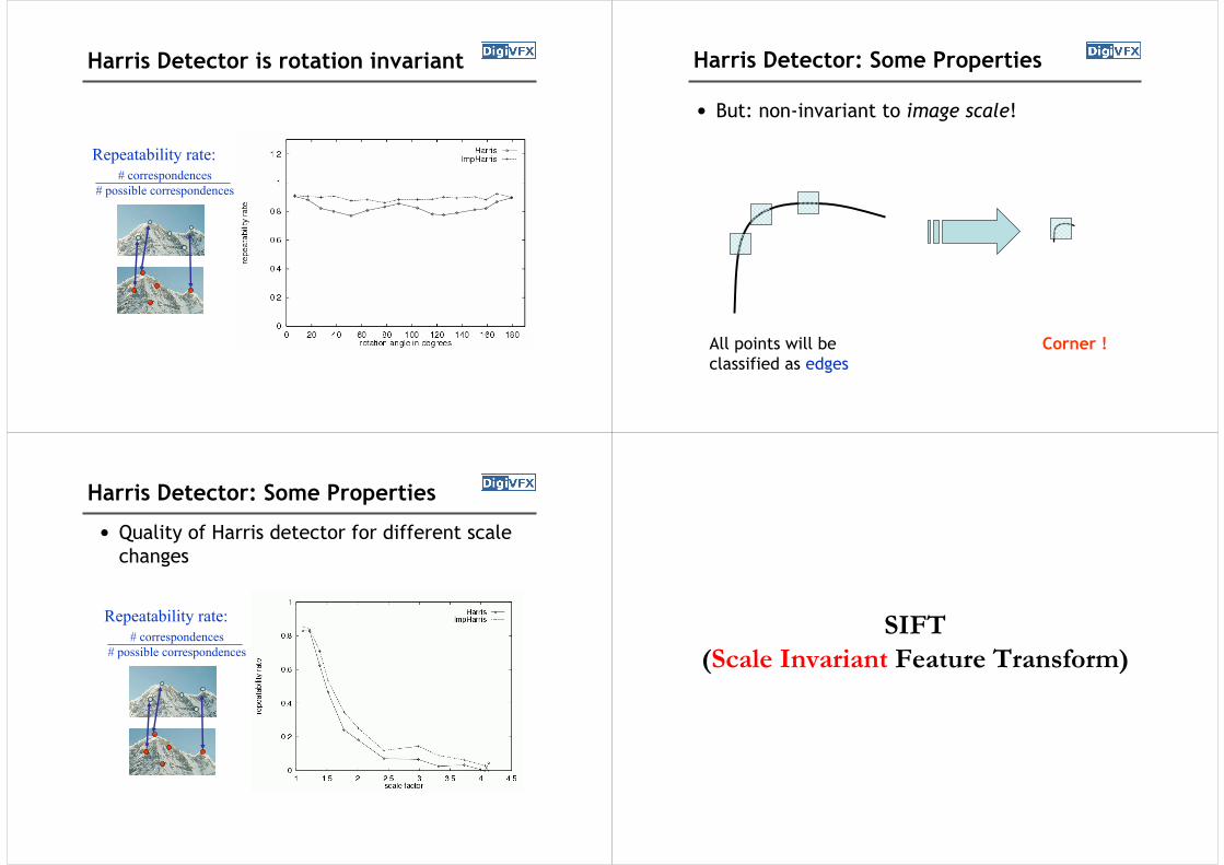
Harris Detector is rotation invariant

Repeatability rate:# correspondences

# possible correspondences

Harris Detector: Some Properties

• But: non-invariant to image scale!

All points will be classified as edges

Corner !

Harris Detector: Some Properties

• Quality of Harris detector for different scale changes

Repeatability rate:# correspondences

# possible correspondences

SIFT (Scale Invariant Feature Transform)

SIFT• SIFT is an carefully designed procedure with

empirically determined parameters for the invariant and distinctive features.

SIFT stages:

• Scale-space extrema detection• Keypoint localization• Orientation assignment• Keypoint descriptor

( )local descriptor

detector

descriptor

A 500x500 image gives about 2000 features

1. Detection of scale-space extrema

• For scale invariance, search for stable features across all possible scales using a continuous function of scale, scale space.

• SIFT uses DoG filter for scale space because it is efficient and as stable as scale-normalized Laplacian of Gaussian.

DoG filtering

Convolution with a variable-scale Gaussian

Difference-of-Gaussian (DoG) filter

Convolution with the DoG filter

Scale spaceσ doubles for the next octave

K=2(1/s), s+3 images for each octave

Keypoint localization

X is selected if it is larger or smaller than all 26 neighbors

Decide scale sampling frequency

• It is impossible to sample the whole space, tradeoff efficiency with completeness.

• Decide the best sampling frequency by experimenting on 32 real image subject to synthetic transformations.

Decide scale sampling frequency

S=3, for larger s, too many unstable features

Decide scale sampling frequency Pre-smoothing

σ =1.6, plus a double expansion

Scale invariance 2. Accurate keypoint localization

• Reject points with low contrast and poorly localized along an edge

• Fit a 3D quadratic function for sub-pixel maxima

Accurate keypoint localization

If has offset larger than 0.5, sample point is changed.

If is less than 0.03 (low contrast), it is discarded.

Eliminating edge responses

r=10

Let

Keep the points with

Keypoint detector

(a) 233x189 image(b) 832 DOG extrema(c) 729 left after peak

value threshold(d) 536 left after testing

ratio of principlecurvatures

3. Orientation assignment

• By assigning a consistent orientation, the keypoint descriptor can be orientation invariant.

• For a keypoint, L is the image with the closest scale,

orientation histogram

Orientation assignment Orientation assignment

Orientation assignment Orientation assignment

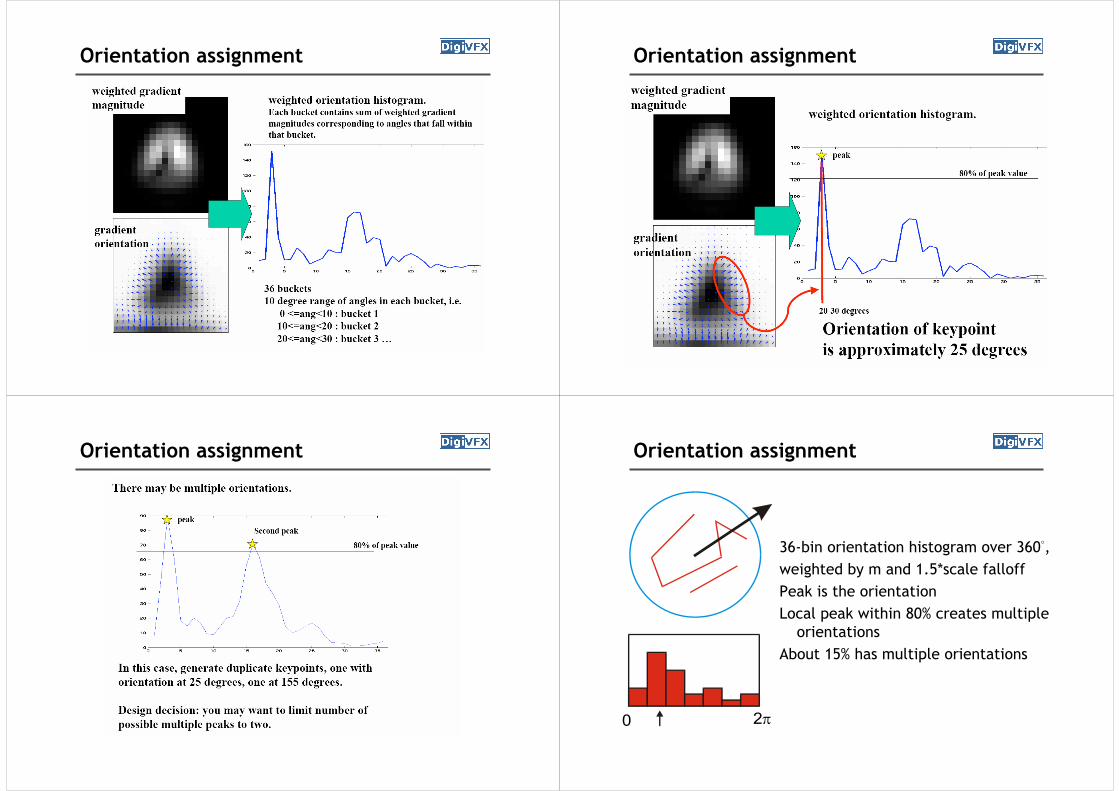
Orientation assignment Orientation assignment

Orientation assignment Orientation assignment

0 2π

36-bin orientation histogram over 360°, weighted by m and 1.5*scale falloffPeak is the orientationLocal peak within 80% creates multiple

orientationsAbout 15% has multiple orientations

Orientation invariance 4. Local image descriptor

• Thresholded image gradients are sampled over 16x16 array of locations in scale space

• Create array of orientation histograms• 8 orientations x 4x4 histogram array = 128 dimensions• Normalized, clip the components larger than 0.2

Why 4x4x8? Sensitivity to affine change

SIFT demo Maxima in D

Remove low contrast Remove edges

SIFT descriptor

Estimated rotation

• Computed affine transformation from rotated image to original image:0.7060 -0.7052 128.42300.7057 0.7100 -128.9491

0 0 1.0000

• Actual transformation from rotated image to original image:0.7071 -0.7071 128.69340.7071 0.7071 -128.6934

0 0 1.0000

SIFT extensions

PCA PCA-SIFT

• Only change step 4• Pre-compute an eigen-space for local gradient

patches of size 41x41• 2x39x39=3042 elements• Only keep 20 components• A more compact descriptor

GLOH (Gradient location-orientation histogram)

17 location bins16 orientation binsAnalyze the 17x16=272-d eigen-space, keep 128 components

Applications

Recognition

SIFT Features

3D object recognition

3D object recognition Office of the past

Video of desk Images from PDF

Track & recognize

T T+1

Internal representation

Scene Graph

Desk Desk

…> 5000images

change in viewing angle

Image retrieval

22 correct matches

Image retrieval

…> 5000images

change in viewing angle+ scale change

Image retrieval Robot location

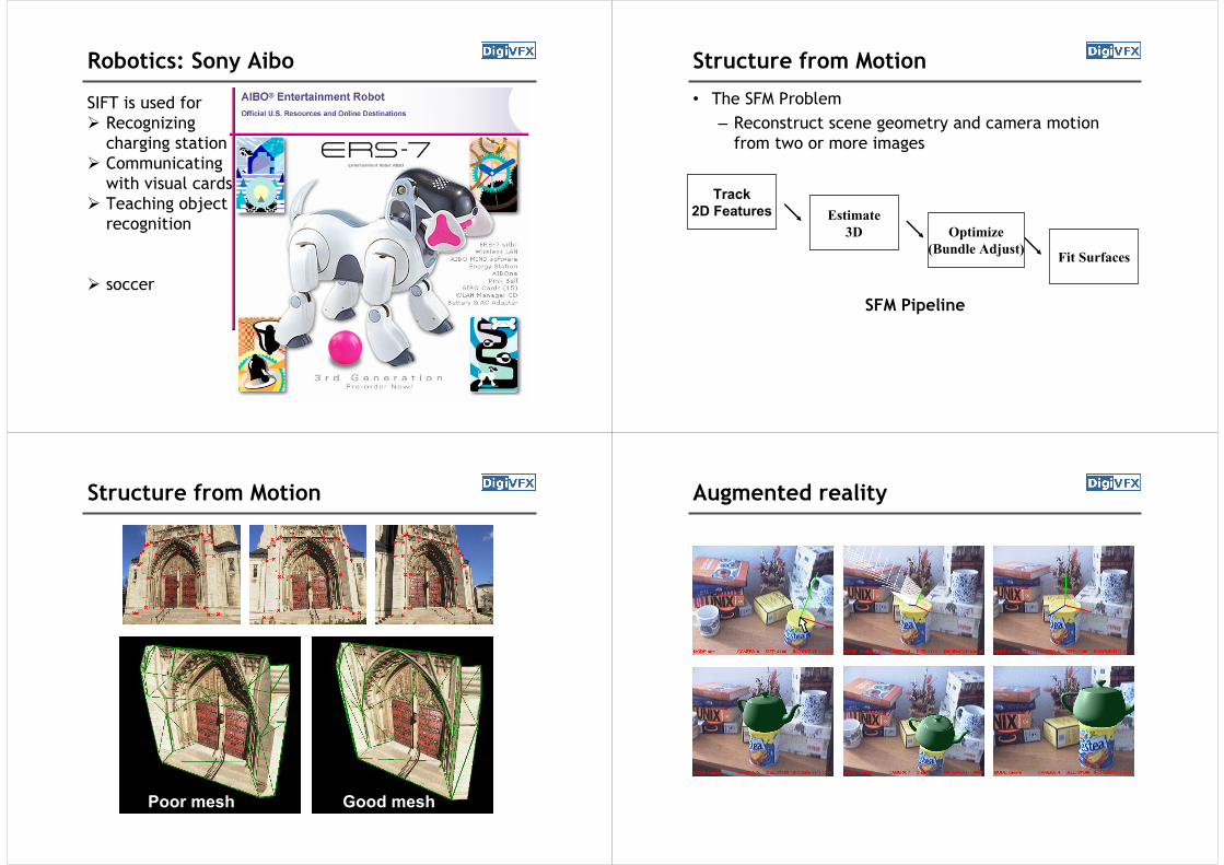
Robotics: Sony Aibo

SIFT is used forRecognizing charging stationCommunicating with visual cardsTeaching object recognition

soccer

Structure from Motion

• The SFM Problem– Reconstruct scene geometry and camera motion

from two or more images

Track2D Features Estimate

3D Optimize(Bundle Adjust) Fit Surfaces

SFM Pipeline

Structure from Motion

Poor mesh Good mesh

Augmented reality

Automatic image stitching Automatic image stitching

Automatic image stitching Automatic image stitching

Automatic image stitching Automatic image stitching

Reference• Chris Harris, Mike Stephens, A Combined Corner and Edge Detector,

4th Alvey Vision Conference, 1988, pp147-151. • David G. Lowe, Distinctive Image Features from Scale-Invariant

Keypoints, International Journal of Computer Vision, 60(2), 2004, pp91-110.

• Yan Ke, Rahul Sukthankar, PCA-SIFT: A More Distinctive Representation for Local Image Descriptors, CVPR 2004.

• Krystian Mikolajczyk, Cordelia Schmid, A performance evaluation of local descriptors, Submitted to PAMI, 2004.

• SIFT Keypoint Detector, David Lowe.• Matlab SIFT Tutorial, University of Toronto.