Embed Size (px)
Citation preview

Progressive damage and failure of unidirectional fiber
reinforced laminates under impact loading with composite
properties derived from a micro-mechanics approach
Gautam Gopinath
Dissertation submitted to the faculty of the Virginia Polytechnic Institute and State University in
partial fulfillment of the requirements for the degree of
Doctor of Philosophy
in
Engineering Mechanics
Romesh C. Batra, Chair
Javid Bayandor
Mark S. Cramer
Scott L. Hendricks
Mark A. Stremler
January 31st, 2011
Blacksburg, Virginia
Keywords: Micro-mechanics, uni-directional fiber reinforced laminates, impact analysis,
damage, failure

Progressive damage and failure of unidirectional fiber reinforced laminates under impact
loading with composite properties derived from a micro-mechanics approach
Gautam Gopinath
(ABSTRACT)
Micromechanics theories have been used to develop macro-level constitutive relations for
infinitesimal elastoplastic deformations of unidirectional fiber reinforced laminates. The matrix
is assumed to be isotropic and deform elasto-plastically and the fibers transversely isotropic and
linear elastically. We have analyzed damage initiation, damage progression, and failure of 16-ply
unidirectional fiber reinforced laminates impacted at normal incidence by a rigid sphere. The
damage is assumed to initiate when at least one of Hashin’s failure criteria is satisfied with the
evolving damage modeled by an exponential relation. Transient three dimensional impact
problems have solved using the finite element method (FEM) by implementing the material
damage model as a user defined subroutine in the FE software ABAQUS. From strains supplied
by ABAQUS the subroutine uses the free shear traction technique and values of material
parameters of the constituents to find average stresses in a FE, and checks for Hashin’s failure
criteria. If the damage has initiated, the subroutine evaluates the damage developed, computes
resulting stresses, and provides them to ABAQUS. The irreversibility of the damage is satisfied
by requiring that the damage evolved does not decrease during unloading. The delamination
failure mode is simulated by using the cohesive zone model and the degradation of material
properties already available in ABAQUS. The computed time histories of the axial load acting
on the impactor are found to agree well with the experimental ones available in the literature.
The effect of stacking sequence in the laminate upon the impact load has been ascertained.

iii
Acknowledgements
I would like to first and foremost acknowledge the support and advice of Prof. Romesh
Batra. I would like to thank him for more than anything else the freedom (with little restriction)
given to me to carry out my research. I owe a lot of my success to his guidance. I would like to
thank Prof. Scott Case for his support. I'm indeed grateful to him. I am also thankful to my
committee members for their valuable time and suggestions.
I am indebted to Mrs. and Mr. Pankaj Kumar and their little one for welcoming me into
their home and treating me as family. No words can express my gratitude towards them and I
will forever cherish their friendship.
I am thankful to Alireza Chadegani for his friendship, company and gossip. He has made
life a little less stressful in the lab. I would also like to thank my friends Phanindra
Tallapraghada, Shakti Gupta, Kaushik Das, Alejandro Pacheco and Anoop Varghese who have
all but become strangers now. I still have some fleeting fond memories of their friendship.
My years in the department has flown by quickly and smoothly for which I would like to
thank all the staff and faculty members of the department.
Last but not the least I would like to show appreciation to my family back home in India
for being patient with me. I am especially grateful to my younger brother for taking over my
responsibilities.
This research was sponsored by the Army Research Laboratory and was accomplished
under Cooperative Agreement Number W911NF-06-2-0014. The views and conclusions
contained in this document are those of the author and should not be interpreted as representing
official policies, either expressed or implied, of the Army Research Laboratory or the U.S.
Government. The work was also partially supported by the Office of Naval Research Grant
N00014-1-06-0567 to Virginia Polytechnic Institute and State University with Dr. Y.D.S.
Rajapakse as the program manager.

iv
Table of Contents
CHAPTER 1: Introduction and literature review 1
1. Introduction 1
2. Objectives and scope of the work 2
3. Historical developments and literature review of homogenization methods 3
4. Review of continuum damage mechanics for fiber reinforced composites 6
5. Organization of the dissertation 8
References 9
CHAPTER 2: Homogenization of elasto-plastic material parameters for
unidirectional fiber-reinforced polymeric composites
13
Abstract 13
1. Introduction 13
2. Elastic material parameters 15
2.1 Preliminaries 15
2.2 Voigt and Reuss rules 18
2.3 Hill’s equivalent energy criterion 18
2.4 Strain concentration tensors 20
2.5 Eshelby’s equivalent inclusion method 20
2.6 Mori-Tanaka method 21
2.7 Self-Consistent method 22
2.8 Aboudi’s method of cells 22
2.9 Free shear traction (FST) method 24
3. Elasto-plastic material parameters 26
3.1 Preliminaries 26
3.2 Infinitesimal elasto-plastic deformations of polymer 26
3.2.1 Pressure independent yielding of polymer 26
3.2.2 Pressure-dependent yielding of polymer 28
3.3 Yield function for unidirectional fiber reinforced polymeric composite (UFPC) 29
3.3.1 Pressure independent yielding of composite 29
3.3.2 Pressure dependent yielding of composite 30
3.4 Determination of elastic-plastic parameters of the UFPC 30
3.4.1 Pressure-independent yield surface 30
3.4.2 Pressure-dependent yield surface 33
4. Numerical results and discussion 34
4.1 Elastic constants for AS4 fibers 34
4.2 Material parameters for PEEK assuming pressure independent yielding 34
4.3 Material parameters for PEEK assuming pressure dependent yielding 37
4.4 Elastic parameters of the composite 40
4.5 Elasto-plastic properties of the composite 46
4.5.1 Validity of the FST approach for elasto-plastic deformations 46
4.5.2 Values of material parameters for the homogenized composite 48
4.5.3 Comparison of results from the FST method with those from the homogenized
composite
49
4.5.4 Dependence of the yield surface upon the fiber volume fraction 53
5. Conclusions 54

v
6. Appendix: comparison of results for elasto-plastic deformations by the M-T and the
FST techniques
56
Acknowledgements 59
References 59
CHAPTER 3: Damage and Failure during Impact Loading of Unidirectional
Fiber-reinforced Laminates
62
Abstract 62
1. Introduction 63
2. Problem Formulation 66
3. Weak Formulation of Governing Equations and the Time Integration Scheme 69
4. Damage and Failure Initiation Criteria 73
5. Damage Evolution 74
6. Element Deletion Criterion 76
7. Cohesive Zone Model for Delamination 76
8. Elastoplastic Deformations of the Matrix 78
9. Micromechanics Approach for Finding Stresses in a Finite Element 79
10. Summary of the Solution Algorithm 80
11.1 Numerical Results and Discussion 80
11.2 Comparison of Computed Results with Experimental Findings 83
11.2.1 Simple quasistatic deformations 83
11.2.2 Impact Loading of a Composite Laminate 90
11.2.3 Evolution of damage during impact loading 101
11.2.4 Effect of laminate stacking sequence on the impact response of the laminate 107
11.2.5 Mesh sensitivity analysis 114 11.2.6 Effect of the rate of evolution of the damage 116
11.3 Effect of presence of the base plate on the response of the composite laminate 118 12. Conclusions 119 Acknowledgements 120 References 120
CHAPTER 4: Conclusions and Contributions 124
1. Conclusions 124
2. Contributions 126
Appendix A 127 ABAQUS input file for the impact analysis of UFPC laminate
Appendix B 130 VUMAT code to analyze damage and failure in UFPC
Appendix C 150 VUMAT code to analyze inelastic deformation in homogenized UFPC
Appendix D 159 MATLAB code for Mori-Tanaka method
Appendix E 162 MATLAB code for Eshelby’s equivalent Inclusion method
vi
List of Figures
Fig. 2-1: Schematic sketch of a unidirectional fiber reinforced lamina with fibers
along the x1 -axis.
16
Fig. 2-2: Left: Cross-section of a UFPC with uniform arrangement of fibers; right:
representation of the cross-section of the RVE by four cells, three of which
are made of the matrix and the fourth one of the fiber.
24
Fig. 2-3: Fiber orientation with respect to the axis of loading, and the material
principal axes ( )321 x,x,x .
31
Fig. 2-4: Computed and experimental axial stress vs. axial strain curves for PEEK
polymer.
35
Fig. 2-5: Effective stress versus effective plastic strain curve for PEEK obtained from
the experimental axial stress versus axial strain curve of [23], and the least
squares fit.
36
Fig. 2-6: Comparison of computed and experimental axial stress vs. axial strain
curves for PEEK polymer deformed in uniaxial tension and compression.
39
Fig. 2-7: Effective stress versus effective plastic strain curve for PEEK obtained from
the experimental axial stress versus axial strain curve of [27].
39
Fig. 2-8: Cross-sections of cubic RVEs with fibers parallel to the -x3 axis; (top):
undeformed configuration, (bottom left) and (bottom right): configurations
obtained by applying displacement field ,0,0xeu 1
0
11= and
,0xe,xeu 1
0
122
0
12= , respectively, to the boundaries.
41
Fig. 2-9: Variation with fv of the elastic modulus E2 = E3 obtained using different
micromechanics approaches; M-T = Mori-Tanaka, FST = free shear
traction, EIM = Eshelby’s inclusion method.
43
Fig. 2-10: Variation with fv of the elastic modulus G12 = G13 obtained using different
micromechanics approaches; M-T = Mori-Tanaka, FST = free shear
traction, EIM = Eshelby’s inclusion method.
44
Fig. 2-11: Variation with fv of the elastic modulus G23 obtained using different
micromechanics approaches; M-T = Mori-Tanaka, FST = free shear
traction, EIM = Eshelby’s inclusion method.
44
Fig. 2-12: Variation with fv of the Poisson’s ratio 12ν obtained using different
micromechanics approaches; M-T = Mori-Tanaka, FST = free shear
traction, EIM = Eshelby’s inclusion method.
45

vii
Fig. 2-13: Variation with fv of the Poisson’s ratio 23ν obtained using different
micromechanics approaches; M-T = Mori-Tanaka, FST = free shear
traction, EIM = Eshelby’s inclusion method.
45
Fig. 2-14: For ,6.0v =f comparison of the computed axial stress-axial strain curves
for the 14o off-axis loading using the FST approach with the experimental
curve of Weeks and Sun [26].
47
Fig. 2-15: For ,6.0v =f comparison of the computed axial stress-axial strain curves
for the 30o off-axis loading using the FST approach with the experimental
curve of Weeks and Sun [26].
47
Fig. 2-16: For ,6.0v =f comparison of the computed axial stress-axial strain curves
for the 45o off-axis loading using the FST approach with the experimental
curve of Weeks and Sun [26].
48
Fig. 2-17: For ,6.0v =f comparison of axial stress - axial strain response for 14o off-
axis loading obtained from the FST method with the response of pressure
insensitive yielding of composites using values of parameters determined
from the two methods.
49
Fig. 2-18: For ,6.0v =f comparison of axial stress - axial strain response for 30o off-
axis loading obtained from the FST method with the response of pressure
insensitive yielding of composites using values of parameters determined
from the two methods.
50
Fig. 2-19: For ,6.0v =f comparison of axial stress - axial strain response for 45o off-
axis loading obtained from the FST method with the response of pressure
insensitive yielding of composites using values of parameters determined
from the two methods.
50
Fig. 2-20: For ,6.0v =f comparison of axial stress - axial strain response for 14o off-
axis loading obtained from the FST method with the response of pressure
sensitive yielding of composites using values of parameters determined
from the two methods.
51
Fig. 2-21: For ,6.0v =f comparison of axial stress - axial strain response for 30o off-
axis loading obtained from the FST method with the response of pressure
sensitive yielding of composites using values of parameters determined
from the two methods.
52
Fig. 2-22: For ,6.0v =f comparison of axial stress - axial strain response for 45o off-
axis loading obtained from the FST method with the response of pressure
52

viii
sensitive yielding of composites using values of parameters determined
from the two methods.
Fig. 2-23: Variation with the fiber volume fraction of parameters A and N appearing in
the strain hardening expression for the composite.
53
Fig. 2-24: Variation with the fiber volume fraction of the parameters A12 and A23
appearing in the yield surface.
54
Fig. 2-25: For ,3.0v =f comparison of the axial stress versus the axial strain curves for
off-axis loading computed using the incremental M-T and the FST methods.
57
Fig. 2-26: For ,4.0v =f comparison of the axial stress versus the axial strain curves
for cyclic loading from the incremental M-T and the FST methods.
58
Fig. 2-27: For ,4.0v =f comparison of the shear stress versus the shear strain curves
computed using the incremental M-T and the FST approaches.
58
Fig. 3-1: Geometric set up for impact test with the impactor shown in green, the
composite laminate in red and the supporting steel plate in blue color.
67
Fig. 3-2: Computed and experimental axial stress vs. axial strain curves for PEEK
polymer.
82
Fig. 3-3: Effective stress versus effective plastic strain curve for PEEK obtained from
the experimental axial stress versus axial strain curve.
83
Fig. 3-4a: Comparison of the experimental and the numerical axial stress versus the
axial strain curves for AS4/PEEK composite for tension test along the fiber
direction.
84
Fig. 3-4b: Comparison of the experimental and the numerical axial stress versus the
axial strain curves for AS4/PEEK composite for compression test along the
fiber direction.
85
Fig. 3-4c: Comparison of the experimental and the numerical axial stress versus the
axial strain curves for AS4/PEEK composite for tension test normal to the
fiber direction.
86
Fig. 3-4d: Comparison of experimental and numerical results for AS4-PEEK
composites for compression test normal to the fiber direction.
87
Fig. 3-4e: Comparison of the experimental and the numerical axial stress versus the
axial strain curves for AS4/PEEK composite for shear deformations in the
plane of the lamina.
88
ix
Fig. 3-5a: Comparison of the experimental and the computed axial stress versus axial
strain curves for AS4/PEEK composite with fibers making an angle of 14o
with the loading axis.
89
Fig. 3-5b: Comparison of the experimental and the computed axial stress versus axial
strain curves for AS4/PEEK composite with fibers making an angle of 30o
with the loading axis.
89
Fig. 3-5c: Comparison of the experimental and the computed axial stress versus axial
strain curves for AS4/PEEK composite with fibers making an angle of 45o
with the loading axis.
90
Fig. 3-6: Stacking sequence of the top half of the symmetric 16 layer composite
laminate.
91
Fig. 3-7: Schematic sketch of the Hertzian contact problem.
93
Fig. 3-8: Comparison of the computed contact force versus the indentation depth
with that obtained from the analytical solution.
94
Fig. 3-9: Comparison of the computed and the experimental time histories of the
contact force.
95
Fig. 3-10a: Fringe plot of stress 11σ at t = 0.55 ms after impact.
96
Fig. 3-10b: Fringe plot of the normal stress 22σ at t = 0.55 ms after impact.
97
Fig. 3-10c: Fringe plot of the normal stress 33σ at t = 0.55 ms after impact.
97
Fig. 3-10d: Fringe plot of the shear stress 12σ at t = 0.55 ms after impact.
98
Fig. 3-10e: Fringe plot of the shear stress 13σ at t = 0.55 ms after impact.
98
Fig. 3-10f: Fringe plot of the shear stress 23σ at t = 0.55 ms after impact.
99
Fig. 3-11a,b:
Fringe plots of internal variables Q1 and Q4 associated with the fiber and the
matrix tensile damage at t = 1.1 ms; and a magnified view of the severely damaged region.
100
Fig. 3-11c,d:
Fringe plots of internal variables Q2 and Q5 associated with the fiber and the
matrix compressive damage at t = 1.1 ms.
100
Fig. 3-11e,f:
Fringe plots of internal variables Q3 and D associated with crush damage
and delamination at t = 1.1 ms.
101

x
Fig. 3-12: Contact force time history plot with points of significance for the damage initiation and propagation.
102
Fig. 3-13a: Fringe plot of internal variable Q2 (fiber compressive damage) at
ms. 0.25t ≈
103
Fig. 3-13b: Fringe plots of internal variables Q2 (fiber compressive damage) and Q4
(matrix tensile damage) at ms. 0.3t ≈
104
Fig. 3-13c: Fringe plots of internal variables Q1 (matrix tensile damage), Q2 (fiber
compressive damage) and Q4 (matrix tensile damage) at ms. 0.4t ≈
105
Fig. 3-13d: Fringe plots of internal variables Q1 (matrix tensile damage), Q2 (fiber
compressive damage), Q4 (matrix tensile damage) and Q5 (matrix
compressive damage) at ms.t 0.52 ≈
106
Fig. 3-13e: Fringe plots of internal variables Q1 (fiber tensile damage) and Q4 (matrix
tensile damage) at ms. 0.55t ≈
107
Fig. 3-14a: Fringe plots of internal variables Q2 (fiber compressive damage), Q5 (matrix
compressive damage), and Q4 (matrix tensile damage) at ms. 0.3t ≈
108
Fig. 3-14b: Fringe plots of internal variables Q1 (matrix tensile damage), Q2 (fiber compressive damage), Q4 (matrix tensile damage) and Q5 (matrix
compressive damage) at s.45.0 m t ≈
109
Fig. 3-14c: Fringe plots of internal variables Q1 (fiber tensile damage) and Q4 (matrix
tensile damage) at s.2 m t ≈
110
Fig. 3-15a: Fringe plots of internal variables Q1 (fiber tensile damage), Q2 (fiber
compressive damage), Q4 (matrix tensile damage), and Q5 (matrix
compressive damage) at s.35.0 m t ≈
111
Fig. 3-15b: Fringe plots of internal variables Q1 (fiber tensile damage), Q2 (fiber compressive damage), Q4 (matrix tensile damage), and Q5 (matrix
compressive damage) at s.9.1 m t ≈
112
Fig. 3-16: Comparison of contact force time histories for three laminate stacking sequences.
113
Fig. 3-17: A graded FE mesh used in the impact analysis of the composite laminate.
114
Fig. 3-18: Contact force time histories plot for three different FE meshes.
115
Fig. 3-19: The axial stress vs. the axial strain curves for different values of m for a composite laminate deformed in uniaxial tension.
116

xi
Fig. 3-20: Comparison of the contact force time histories for m =4 and 100.
117
Fig. 3-21: Fringe plot of the normal displacement (u3) on the back surface of the composite laminate
119
List of Tables
Table 2-1: Elastic constants of AS-4 carbon fibers.
34
Table 2-2: Values of material parameters for the matrix.
56
Table 2-3: Values of material parameters for the carbon fibers.
56
Table 3-1: Values of material parameters for the AS4 fiber [26].
81
Table 3-2: Values of material parameters for PEEK polymer [27].
81
Table 3-3: Values in GPa of strength parameters for the AS4/PEEK composite
with 60% volume fraction of fibers [28].
81
Table 3-4: Values of interfacial strength parameters for the composite laminate [31].
92
Table 3-5: Elastic properties of the indenter and the plate material.
93
Table 3-6: Summary of results for the three laminate sequences under impact loading.
113
Table 3-7: Summary of results for the 2S/90] /45 /0 [-45 laminate obtained with three
different meshes.
115
Table 3-8: Summary of results for the 2S/90] /45 /0 [-45 laminate for m = 4 and 100. 118
1
CHAPTER 1: Introduction and literature review
1. Introduction
Present day materials used in industry are required to meet many design specifications
which are often not fulfilled by conventional monolithic materials. Composites are a very good
alternative and offer a number of advantages over their conventional counterparts. Typically a
composite is made of two or more materials and its constituents are tailored to meet the design
specifications. For example, to optimize the aerodynamics of flight, the wings of combat aircraft
have to be shaped intricately; apart from this they require varied stiffness along their wingspan.
If metal parts were to be used they need to be machined to the required specifications as one
single piece, and if multiple parts are used they are usually fastened. This makes it cumbersome
and costs make their use prohibitive. Using composites, which generally are lighter than metals,
a designer has greater flexibility because the strength and the stiffness of the structure can be
tailored by stacking laminate plies in localized areas and along preferred orientations. Also, with
the advances made in the manufacturing processes complex shapes can now be cured in
autoclaves. Composites have significantly influenced some industries, nearly 10% by weight of
current day commercial aircrafts and cars are made of composites. The airbus 350 aircraft and
the Boeing 787 Dreamliner have nearly 50% composite by weight. The ever increasing growth
in composites usage and their wide applicability means that they need to be studied and analyzed
thoroughly.
The dissertation deals with the analysis of composites which exhibit more than one
spatial scale. To understand and clarify the above statement, consider the makeup of a typical
bullet proof vest. At the micro-scale the vest is made of fine polymeric fibers typically only a
few micrometers in diameter. At the next higher scale are the woven fiber bundles, which consist
of a collection of fibers bonded together and are typically in the millimeter range. Finally, we
have the woven laminate structure. The vest thus exhibits a different structure at each spatial
scale and hence may be classified as multi-scaled. In general, materials that appear to be
homogeneous at the macro-scale exhibit heterogeneity at the micro-structural level. Even if one
considers a defect free single crystal whose microstructure is uniform it is ultimately discrete at
the atomic scale.

2
It is well known that the macroscopic behavior of a heterogeneous material is
significantly influenced by its microstructure. For example, it is seen that the addition of rigid
particles to a polymer can increase its stiffness, and improve creep resistance and fracture
toughness [1]. The mechanical properties are also influenced by the size, the shape, the aspect
ratio and the distribution of reinforcing particles [1]. In ceramic matrix composites the toughness
is increased by the addition of soft inclusions. In a ceramic matrix composite a propagating crack
when intercepted by a ductile inclusion causes it to deform plastically, blunts the crack front and
thus dissipates energy [2]. In steel it is seen that the elongation of non-metallic inclusions can
reduce its ductility, failure strain and fracture toughness, but through shape control of the non-
metallic inclusions such deleterious effects can be greatly reduced [3]. Since the micro-structure
has a profound effect on the macroscopic behavior it is important to study how the
microstructure influences the macroscopic behavior. This forms the basis of the dissertation, that
is, to be able to predict the macroscopic behavior using information available at the constituent
level.
It is impractical and unfeasible to study deformations of each constituent in
heterogeneous materials that exhibit multiple spatial scales through experiments, primarily
because of the number of variables that can influence the outcome, and the difficulty in
monitoring deformations at the constituent level. These problems are thus best studied through
numerical investigations. Also, since the problems being analyzed span several spatial scales it is
computationally expensive to carry out numerical simulations that account for the complete
heterogeneous structure of the body. Approximate methods need to be devised that account for
micro-structural details and bridge different spatial scales; such approximate techniques are
called homogenizing schemes.
2. Objectives and scope of the work
Inelastic behavior in fiber reinforced composites is primarily due to inelastic
deformations of the matrix [4, 5]. Though fibers exhibit strain rate dependent elastic and strength
properties their effects could be considered negligible as compared to that of the matrix. To
analyze the inelastic behavior in AS4-PEEK composites Weeks and Sun [5] developed a
macroscopic viscoplastic model based on an earlier work of Sun and Chen [6] by assuming that
3
the composite remains elastic when loaded along the fiber direction but can undergo
plastic/visco-plastic pressure-independent deformations otherwise. Zhao et al. [7] modeled AS4-
PEEK composite as an elastic-plastic material with nonlinear hardening and used the yield
function developed by Sun and Chen [6]. The advantage of using a macro-model is that it is
computationally efficient but a major short coming is that it relies on data from experimental off-
axis loading of fiber reinforced composites to establish the parameters for the macro-model.
The objective of the present work is to use a micro-mechanics based approach to first
derive values of macroscopic material parameters and then use them to analyze failure and
damage at the macroscopic level. The micro-mechanics approach accounts for the inelastic
behavior of the matrix and hence of the composite. Failure and damage in the composite is
considered using continuum damage mechanics approach. The micro-mechanics method and the
failure/damage model is integrated into a finite element setting so as to be able to solve problems
under general loading conditions. The validity of the approach is tested by comparing simulated
results with experimental findings.
3. Historical developments and literature review of homogenization methods
Some of the earliest work in this area dates back to the early twentieth century when
Voigt and Reuss found the effective properties of a heterogeneous material based on the volume
fractions of its constituents. Hill [8] proved that the elastic constants obtained through the Voigt
and the Reuss rules are the upper and the lower bounds of the effective properties of the
heterogeneous material. The bounds are narrow when properties of the individual constituents
are close to each other but as the difference between the properties increases so does the
difference in the two bounds. Though these rules are still used today, they are of only limited
use as they are valid only under dilute concentrations of inclusions in the composite. Hashin [9,
10, 11] in a series of papers developed variational principles for heterogeneous materials and
derived bounds for the effective elastic properties of the homogenized body; these bounds are
tighter than those derived by Hill and are commonly referred to as the Hashin-Shtrikman bounds.
Willis [12] developed the Hashin-Shtrikman bounds in a generalized way using Green’s function
approach and found the effective thermal conductivity and elastic properties of a heterogeneous
material containing spheroidal inclusions, cracks and needle shape inclusions. For a more

4
comprehensive review of this area one should refer to Torquato [13], and for details on bounds
for non-linear behavior one can refer to works by Talbot and Willis [14], Ponte Castaneda [15],
Suquet [16] and references therein.
The Mori-Tanaka [17, 18] (M-T) method is often used to estimate the effective properties
of composites. In spite of its limitations [19] it has gained popularity primarily because of the
ease with which it can be implemented in a computer program, and the explicit relations one can
derive for effective properties provided that the deformations are linear elastic and inclusions
have simple geometric shapes. Other micro-mechanical models which could be classified in the
same class as the M-T method include the equivalent inclusion method [20], the self consistent
method introduced by Hill [21], the double inclusion method developed by Nemat-Nasser [22],
and the transformation field analysis developed by Dvorak and Benveniste [23] and Dvorak[24].
The major limiting factors of the methods listed in the preceding paragraph are that they
are restricted to small strains. Since they depend on the use of the Eshelby tensor to determine
the effective properties, the shapes of inclusions need to be ellipsoidal. The homogenizing
methods are of course not limited to the elastic regime and these have been extended to study in-
elastic deformations using the M-T scheme. Tandon and Weng [25] used the M-T scheme to
homogenize composites in which matrix undergoes plastic deformations (based on the J2 flow
theory), and Lagoudas et al. [26] applied the M-T method to study the elasto-plastic behavior of
metal matrix composites. Jiang and Batra [58] have used the energy equivalence approach and
the M-T theory to deduce effective moduli of epoxies containing piezoelectric and shape
memory inclusions. In recent years there has been a growing interest in extending the M-T
scheme to study damage and more specifically to study de-bonding between the inclusion and
the matrix. The method adopted by Baney et al. [27] assumes that de-bonding follows a Weibull
probability distribution function and the failure is governed by the tri-axial tensile state at the
inclusion matrix interface. Qu [28] developed relations for effective stiffness of a heterogeneous
system undergoing de-bonding by explicitly considering the displacement jump across the
interface between the inclusion and the matrix using the M-T scheme. Dvorak and Zhang [29]
and Matous [30] have used the transformation field analysis to study the effect of de-bonding.

5
Gartener [59] has generalized Aboudi’s [60] method of cells to consider debonding between the
matrix and the fibers.
Homogenization of composites can also be carried out using mechanics of material
approach. Ha et al. [31] have derived explicit expressions for compliance/stiffness matrix for
fiber reinforced composites by assuming axial strains along the fiber direction to be equal in both
the matrix and fiber and along the transverse directions stresses in the fiber are in some
proportion to the those in the matrix, with the proportionality factors to be determined from the
experimental data. The method of cells developed by Aboudi [60] is another well established
micro-mechanics approach used to model both continuous and short fiber reinforced composites.
Apart from modeling elastic behavior of composites, Aboudi [32] has modified the approach to
account for inelastic deformations in composites. In this approach, a representative volume
element (RVE) is comprised of four parallelepiped cells; three cells are made of the matrix and
one of the fiber. The volume fraction of the fiber cell equals the volume fraction of fibers in the
composite. Based on continuity and equilibrium conditions satisfied on the average across
interfaces between adjacent cells, explicit constitutive equations for the composite are derived.
Aboudi has modeled inelastic deformations in the composite by assuming fibers can undergo
only elastic deformations while the matrix can undergo inelastic deformations. Robertson and
Mall [33] relaxed the continuity of tangential tractions across the interfaces between adjacent
cells, and showed through numerical experiments that this assumption does not affect values of
the effective material properties. Pecknold and Rahman [34, 35] have developed a three-
dimensional (3D) micromechanical model similar to that developed by Aboudi [32] but the RVE
considered is divided into 3 sub-cells consisting of a fiber region and two matrix regions. In
Aboudi’s method of cells, the deduced effective properties of the composite are independent of
the shapes of fibers since the RVE has their equivalent volume fraction rather than the actual
shapes as in the M-T scheme.
The micro-mechanics approaches stated above are restrictive in the sense that they cannot
be applied for large deformations and, in general, for inclusions of irregular shapes. These also
do not account for the spatial distribution of the inclusions. This can, however, be overcome if a
numerical approach is adopted. A finite element scheme is a preferred method to solve such

6
problems, though the Fast Fourier transform (FFT) method has also been used [36, 37]. To carry
out the homogenization process using the finite element method (FEM) RVEs of both the
inhomogeneous and the heterogeneous materials are meshed, displacement, traction and periodic
boundary conditions are applied on the RVE boundaries and Hill’s energy equivalence theorem
is used to obtain the homogenized elastic constants. In periodic boundary conditions, opposite
surfaces of the RVE conform to the same deformed shape. From the solution of the problem
associated with the RVE, the local/effective stiffness and the average/effective stress and strain
can be calculated. In the method of asymptotic expansion, periodic boundary conditions are
applied on the surfaces of the RVE to homogenize the heterogeneous material. For an exhaustive
analysis of this subject one can refer to works by Guedes and Kikuchi [38] and Bensoussan et al.
[39]. Homogenization can also be achieved by applying the boundary conditions on the RVE
through Lagrange multipliers, details of such an analysis can be found in the works of Miehe
[40] and Koch and Miehe [41]. Another approach proposed by Kouznetsova et al. [42] and Smit
et al. [43] can be applied only to 2D problems. It involves applying tie constraints to opposite
edges of the RVE so that the deformed edges on opposite sides of the RVE conform to the same
shape. Though the computational methods offer greater flexibility as compared to the micro-
mechanics based approaches in terms of the complexity of the problem that can be solved, they
are a huge burden on the computational resources and remain impractical to study large practical
problems.
4. Review of continuum damage mechanics for fiber reinforced composites
Some of the earliest work on damage in fiber reinforced laminated composites was
reported by Ladeveze and Dantec [44]. Their theory assumes damage to be uniform throughout
the thickness of each individual lamina that makes up the composite. It is considered to be meso-
scale because it falls between the micro-scale damage analysis of its constituents (fibers and
matrix) and macro-scale damage analysis of laminates [45]. In this method internal variables are
used to degrade the elastic properties of the composite. Ladeveze and Dantec’s damage model
[44] at the ply level accounts for tensile and compressive fiber damage and matrix cracking.
Plasticity type equations are also used to account for permanent deformations due to shear
loading. Johnson [46] has used this model to study damage in fabric composites under impact
loads. A major short coming in utilizing this model is that it requires a large number of input

7
parameters that need to be determined experimentally at specific fiber orientations. Further it
assumes plane stress conditions and numerical simulations using the FEM are restricted to shell
elements.
Hassan and Batra [47] have used three internal variables to account for damage due to
fiber breakage, matrix cracking and fiber matrix debonding with the damage applied locally to a
constituent. Experimental stress strain curves are used to extract and derive the
phenomenological expressions relating damage variables with their corresponding conjugate
forces. This approach enables one to compute the energy dissipated in each failure mode.
Donadon et al. [48] have developed a 3D failure model to predict damage in composite
structures subjected to multi-axial loading. To avoid strain localization and mesh dependence
due to damage a smear crack approach has been incorporated into the problem formulation.
Parameters for the damage law were obtained through experimental data, details of which can be
found in [49].
Clegg et al. [50] have implemented a damage model for hyper-velocity impacts in
AUTODYN. To account for the nonlinear behavior in the fiber reinforced composite it is
assumed that the composite undergoes plastic deformations having a yield surface which is
quadratic in stress. Softening behavior in the composite is accounted for by using damage
mechanics with the damage surface defined in terms of the Cauchy stresses and damage
variables. The evolutions of damage variables are expressed as a function of the critical strain,
the fracture energy, the fracture stress and a local characteristic dimension.
Maa and Cheng [51] have computed the tensile strength of laminated composites
containing a circular hole by using a damage model and three failure modes, namely, fiber
breakage, matrix cracking and interface debonding. To account for nonlinear hardening behavior
during shear loading a phenomenological model on the lines of Ramberg-Osgood plasticity
relation was used to express the shear stress-the shear strain relation. The parameters for the
model were obtained through curve fitting.

8
Hou et al. [52] have considered fiber tensile failure, tensile matrix cracking, matrix
crushing and delamination to study impact analysis of fiber reinforced composites. Chang-Chang
failure criteria was modified by incorporating in the failure modes additional terms depending
upon the shear stresses. Once failure criteria are met stress components associated with the
different failure modes are reduced to zero.
Matzenmiller et al. [53] assumed that damage initiates at a point when one of Hashin’s
failure criteria is met there and proposed a damage evolution law that is an exponential function
of stresses. The elastic properties are progressively decreased with the evolution of damage, and
this model is often referred to as the MLT damage model. The MLT approach has also been
used to study damage in woven fabric composites, e.g., Xiao et al. [54] have used it to study
damage during quasi-static punch test for woven fabric composites. Williams and Vaziri [55]
have evaluated the effectiveness of the MLT damage model under impact loads by studying
damage in carbon fiber reinforced plastics, and Xiao [56] has used it to study damage during
crushing of hollow tubes. Huang and Lee [57] have used Hashin and Yeh’s delamination failure
criteria to analyze crushing of fiber reinforced composites plates. The evolution of damage
variables is proportional to the reciprocal of the failure factors rather than an exponential
function of damage used in the MLT approach.
In the present work the MLT damage model is used to delineate damage at a point and
then degrade the material properties, and a micro-mechanics approach is adopted to find the
effective material properties of a point from those of the constituents.
5. Organization of the dissertation
The rest of the dissertation is organized as follows. The second chapter focuses on using
micro-mechanics theories to derive mechanical properties of a unidirectional fiber reinforced
composite from those of its constituents, and the third chapter on analyzing deformations of
laminated composite plates under impact loading. Major conclusions and contributions from this
work are summarized in the fourth chapter.

9
References
1 Ahmed S., Jones F. R., A review of particulate reinforcement theories for polymer
composites. Journal of Materials Science, 25, 1990, 4933-4942.
2 Sun X., Yeomans J. A., Influence of particle size distribution on ductile-phase toughening in brittle materials. Journal of American Ceramic Society, 79, 1996, 562-564.
3 Paul S. K., Roy A., Influence of inclusion characteristics on the formability and toughness properties of a hot-rolled deep-drawing quality steel. Journal of Materials Engineering and
Performance, 6, 1997, 27-34.
4 Goldberg R. K., Strain rate dependent deformation and strength modeling of a polymer matrix composite utilizing a micromechanics approach. NASA/TM—1999-209768.
5 Weeks C.A., Sun C.T., Modeling non-linear rate-dependent behavior in fiber-reinforced
composites. Composite Science and Technology, 58, 1998, 603–11.
6 Sun, C. T., Chen, J. L., A simple flow rule for characterizing nonlinear behavior of fiber
composites. Journal of Composite Material, 23, 1989, 1009-1020.
7 Zhao G. H., Tong J. W., Shen M., Numerical analysis and experimental validation of interlaminar stresses of quasi-isotropic APC-2/AS-4 laminate with a central hole loaded in
tension. Journal of Thermoplastic composite materials, 1, 2009,1-21.
8 Hill R., Elastic behavior of reinforced solids: Some theoretical principles. Journal of the mechanics and Physics of Solids, 11, 1963, 357-372.
9 Hashin Z., Shtrikman S., On some variational principles in anisotropic and
nonhomogeneous elasticity. Journal of the mechanics and Physics of Solids, 10, 1963, 335-342.
10 Hashin Z., Shtrikman S., A variational approach to the theory of the elastic behavior of Polycrystals. Journal of the mechanics and Physics of Solids, 10, 1963, 343-352.
11 Hashin Z., Shtrikman S., A variational approach to the theory of the elastic behavior of
multiphase materials. Journal of the mechanics and Physics of Solids, 11, 1963, 127-140.
12 Willis J. R., Bounds and self consistent estimates for the overall properties of anisotropic composites. Journal of the mechanics and Physics of Solids, 25, 1977, 185-202.
13 Torquato S., Random heterogeneous media. Springer-Verlag, New York, 2002.
14 Talbot D. R. S, Willis J. R., Variational principles for inhomogeneous nonlinear media. Journal of Applied mechanics, 35, 1985, 39-54.
15 Ponte Castaneda P., New variational principles in plasticity and their application to
composite materials. Journal of the mechanics and Physics of Solids, 40, 1992, 1757-1788.
16 Suquet P. M., Continuum micro-mechanics. Springer-Verlag, New York, 1997.

10
17 Mori T., Tanaka K., Average stress in matrix and average elastic energy of materials with mis-fitting inclusions. Acta Metallurgica, 21, 1973, 571-574.
18 Benveniste Y., A new approach to the application of the Mori-Tanaka’s theory in composite materials. Mechanics of Materials, 6, 1987, 147-157.
19 Christensen R. M., A critical evaluation of a class of micromechanics models. Journal of
the mechanics and Physics of Solids, 38, 1990, 379-404.
20 Pyrz R., Lecture notes on composite materials- current topics and achievements. De- Borst R., Sadowski T., editions. Springer-Science, New York, 2008, 77-97.
21 Hill R., A self consistent mechanics for composite materials. Journal of the mechanics and Physics of Solids, 13, 1965, 213-222.
22 Hori M., Nemat-Nasser S., Double inclusion model and overall multi-phase composites.
Mechanics of Materials, 14, 1993, 189-206.
23 Dvorak G. J., Benveniste Y., On transformation strains and uniform fields in multi-phase elastic media. Proceedings of the Royal society of London A, 437, 1992, 291-310.
24 Dvorak G. J., Transformation field analysis of inelastic composite materials. Proceedings of the Royal society of London A, 437, 1992, 311-327.
25 Tandon G.P., Weng R. L., A theory of particle reinforced plasticity. Journal of Applied
Mechanics, 55, 1988, 126-135.
26 Lagoudas D.C., Gavazzi A.C., Nigam H., Elastoplastic behavior of metal matrix composites based on incremental plasticity and the Mori-Tanaka averaging scheme.
Computational Mechanics, 8, 1991, 192-203.
27 Baney J. M., Zhao Y. H., Weng G. J., Progressive debonding of aligned oblate inclusions
and loss of Stiffness in a brittle matrix composite. Engineering Fracture Mechanics, 53, 1996, 897-910.
28 Qu J., The effect of slightly weakened interfaces on the overall elastic properties of
composite materials. Mechanics of Materials, 14, 1993, 269-281.
29 Dvorak G. J., Zhang J., Transformation field analysis of damage evolution in composite materials. Journal of the Mechanics and Physics of solids, 49, 2001, 2517-2541.
30 Matous K., Damage evolution in particulate composite materials. International Journal of Solids and Structures, 40, 2003, 1489-1503.
31 Ha S. K., Wang Q., Chang F. K., Modeling the viscoplastic behavior of fiber-reinforced
thermoplastic matrix composites at elevated temperatures. Journal of composite materials, 25, 1991, 334-374.
32 Aboudi J., Closed form constitutive equations for metal matrix composites. International
Journal of Engineering Science, 25, 1987, 1229-1240.

11
33 Robertson D. D., Mall S., Micromechanical analysis for thermo-viscoplastic behavior of unidirectional fibrous composites. Composites Science and Technology, 50, 1994, 483-
496.
34 Pecknold D. A., Rahman S., Application of a new micromechanics based homogenization
technique for nonlinear compression of thick-section laminates. Compression response of composite structures. ASTM, Philadelphia, 1994, 34-54.
35 Pecknold D. A., Rahman S., Micromechanics-based structural analysis of thick laminated
composites. Computers and structures, 51, 1994, 163-179.
36 Moulinec H., Suquet P., A numerical method for computing the overall response of non-linear composites with complex microstructure. Computer methods in applied mechanics
and engineering, 157, 1998, 69-94.
37 Michel J.C., Moulinec H., Suquet P., Effective properties of composite materials with
periodic microstructure: A computational approach. Computer methods in applied mechanics and engineering, 172, 1999, 109-143.
38 Guedes J. M., Kikuchi N., Preprocessing and post-processing for materials based on the
homogenization method with adaptive finite element methods. Computer methods in Applied Mechanics and Engineering, 83, 1990, 143-198.
39 Bensoussan A., Lions J.L., Papanicolaou G., Asymptotic analysis for periodic structures.
North-Holland Publishing Company, New York, 1978.
40 Miehe C., Koch A., Computational micro-to-macro transitions of discretized micro-
structures undergoing small strains. Archive of Applied Mechanics, 72, 2002, 300-317.
41 Miehe C., Computational micro-to-macro transitions for discretized micro-structures of heterogeneous materials at finite strains based on minimization of averaged incremental
energy. Computer methods in applied mechanics and engineering, 192, 2003, 559-591.
42 Kouznetsova V., Brekelmans W. A. M., Baaijens F.P.T. An approach to micro-macro modeling of heterogeneous materials. Computational mechanics, 27, 2001, 37-48.
43 Smit R. J. M., Brekelmans W. A. M., Meijer H. E. H., Prediction of mechanical behavior of nonlinear heterogeneous systems by multi-level finite element modeling. Computer
methods in Applied Mechanics and Engineering, 155, 1998, 181-192.
44 Ladeveze P., Dantec E. Le., Damage modeling of the elementary ply for laminated composites. Composites Science and Technology, 43, 1992, 257-267.
45 Herakovich C. A., Mechanics of fibrous composites. John Wiley publication, New York,
1998.
46 Johnson A. F., Modeling fabric reinforced composite under impact loads. Composites A,
32, 2001, 1197-1206.
47 Hassan N. M., Batra R. C., Modeling damage in polymeric composites. Composites B, 39,

12
2008, 66–82.
48 Donadon M. V., de.Almeida S. F. M, Arbelo M. A., de Faria A. R.. Three-dimensional Ply
failure model for composite structures. International Journal of Aerospace Engineering, 2009, 2009, 1-22.
49 Donadon M. V., Iannucci L., Falzon B. G., Hodgkinson J. M., and de Almeida S. F. M., A
progressive failure model for composite laminates subjected to low velocity impact damage. Computers and Structures, 86, 2008, 1232–1252.
50 Clegg R. A., White D. M., Riedelb W., Harwick W., Hypervelocity impact damage
prediction in composites: Part I—material model and characterization. International Journal of Impact Engineering, 33, 2006, 190–200.
51 Maa R. H., Cheng J. H., A CDM-based failure model for predicting strength of notched composite laminates. Composites B, 33, 2002, 479–489.
52 Hou J. P., Petrinic N., Ruiz C., Hallett S. R., Prediction of impact damage in composite
plates. Composites B, 33, 2002, 479–489.
53 Matzenmiller A., Lubliner J., Taylor R. L., A constitutive model for anisotropic damage in fiber composites. Mechanics of Materials, 20, 1995, 125-152.
54 Xiao J. R., Gama B. A., Gillspie J. W., Progressive damage and delamination in plain weave S-2 glass/SC-15 composites under quasi-static punch shear loading. Composites
Structures, 78, 2007, 182-196.
55 Williams K. V., Vaziri R., Application of a damage mechanics model for predicting the impact response of composite materials. Composites and Structures, 79, 2001, 997-1011.
56 Xiao X., Modeling energy absorption with a damage mechanics based composite material
model. Journal of Composite Materials, 43, 2009, 427-444.
57 Huang C. H., Lee Y. J., Experiments and simulation of the static contact crush of
composite laminated plates. Composite Structures, 61, 2003, 265–270.
58 Jiang B., Batra R. C., Micromechanical modeling of a composite containing piezoelectric and shape memory alloy inclusions. Journal of Intelligent material systems and structures,
21, 2001, 165-182.
59 Gardner J. P., Micromechanical modeling of composite materials in finite element analysis using an embedded cell approach. M. Sc. thesis, M.I.T., Cambridge, Massachusetts, 1994.
60 Aboudi J., Mechanics of composite materials. Elsevier science publication, Amsterdam,
1991
13
CHAPTER 2: Homogenization of elasto-plastic material parameters for unidirectional
fiber-reinforced polymeric composites
Abstract
After reviewing several micromechanical theories for determining values of elastic
parameters for a unidirectional fiber reinforced polymeric composite (UFPC), we find values of
these parameters using four such theories for an AS4/PEEK composite. We also study elastic-
plastic deformations of the UFPC in which fibers are assumed to deform elastically but the
matrix undergoes both elastic and plastic deformations. The matrix plastic deformations are
considered by using the associative flow rule of plasticity. Both the pressure-independent von
Mises yield surface and the pressure-dependent Drucker-Prager yield surfaces are employed to
model elastic-plastic deformations of the polymer and the composite. In both cases the strain
hardening of the matrix is considered and values of material parameters for the matrix are
obtained by computing the effective stress versus the effective plastic strain curves from
experimental uniaxial stress-strain curves. Values of parameters in the yield surface for the
UFPC in terms of those of the matrix and the fiber and the volume fraction of fibers are found by
using a micromechanical theory. Wherever possible, the computed results are compared with the
corresponding experimental results available in the literature.
Key words: Homogenization, micro-mechanics, elastic-plastic deformation, fiber reinforced
composites
1. Introduction
Composite materials are being increasingly used in several applications because of their
high specific strength, and they can be engineered to attain desired mechanical properties in
specific directions. For example, the optimization of the aerodynamics of a flight of an aircraft
may require that the wings be shaped intricately and their stiffness suitably varied along the
wingspan. If the wings were made of a metal then different parts will need to be precisely
machined and fastened. Most metals are isotropic materials meaning they have same properties
in all directions. Thus the thickness of a part will need to be varied to get the desired stiffness in
a particular direction. When using composites, one can exploit their directional properties and

14
still get a uniform thickness but adjust stiffness in different directions. Moreover, the mass
density of a composite is generally less than that of a metal, and complex shapes can be cured in
an autoclave.
Composites being inhomogeneous materials provide challenges in design since their
failure mechanisms are not well understood. Furthermore, for design purposes, one needs to find
properties of a homogeneous material equivalent in mechanical response to the composite.
Several homogenization techniques have been proposed in the literature to find mechanical
properties of the composite from those of its constituents when the deformations are linear
elastic; for example, see books by Torquato [1], Suquet [2], Bensoussan et al. [3], Nemat-Nasser
and Hori [4], Mura [5], Aboudi [6], Tsai and Hahn [7], Hyer [8], and Reifsnider and Case [9],
and the review paper by Charalambakis [10]. In contrast to the micromechanical theories Love
and Batra [11] numerically simulated plane strain deformations of a mixture of a metal matrix
composite with circular cylindrical fibers by keeping edges of the cross-section plane and
deduced values of the elastic and the plastic parameters at different strain rates by assuming that
under quasistatic deformations the yield stress of the composite is given by the rule of mixtures.
The unidirectional fiber reinforced polymeric composites (UFPCs) with fibers in a ply laid
parallel to each other may undergo inelastic deformations due to unexpected large loads applied
to them. Young’s modulus of a lamina in the direction of fibers is considerably more than that in
any other direction. Most fibers undergo infinitesimal elastic deformations prior to failure but
the matrix bonding the fibers can deform inelastically either because deformations of the matrix
are large or its yield stress is very small.
Bridgman [12] experimentally showed that the hydrostatic pressure does not affect plastic
deformations of metals. However, mechanical deformations of some polymers have been shown
to be influenced by the hydrostatic pressure. Thus the yield surface for such a polymer should
depend upon the hydrostatic pressure; this dependence has been considered, among others, by
Caddell et al. [13], and Hu and Pae [14]. Here we consider one such yield criterion for the
matrix and account for its strain hardening. The yield surface for the UFPC is deduced by
making the following assumptions: (i) the UFPC is a transversely isotropic material with the

15
fiber axis as the axis of transverse isotropy, (ii) there is no plastic deformation in the direction of
fibers, and (iii) fibers deform elastically. We use a micromechanical theory to quantify the
dependence of values of material parameters appearing in the yield function as a function of the
volume fraction of fibers and mechanical properties of the matrix and the fibers. The functional
dependence of the effective stress of the composite upon the effective plastic strain (i.e., the
strain hardening effect) is taken to be similar to that of the matrix.
The rest of the paper is organized as follows. We review in Section 2 eight
micromechanical theories to determine elasticities of the composite from those of the fibers and
the matrix, and the volume fraction of fibers. Section 3 describes pressure-dependent and
pressure-independent yield surfaces for the matrix and the UFPC, and techniques to evaluate
various material parameters appearing in the yield surface of the UFPC from those of the fiber
and the matrix. For an AS4/PEEK composite, the computed numerical results are compared with
the experimental findings available in the literature in Section 4, and conclusions of this study
are summarized in Section 5 where values of material parameters in the yield surface for the
UFPC as a function of the volume fraction of fibers are given. We have compared in the
appendix results of elastic plastic deformations of the UFPC from the incremental Mori-Tanaka
and the FST methods. These results show that for in-plane shear deformations the two
micromechanics approaches give different values of the yield stress and the strain-hardening
modulus.
2. Elastic material parameters
2.1 Preliminaries
In this section we review eight micromechanics theories that have been proposed to
derive effective properties of UFPCs from those of their constituents. We assume that fibers are
straight circular cylinders and the fiber material is transversely isotropic with the fiber axis as the
axis of transverse isotropy. Thus we need values of five elastic moduli to characterize the fiber
material. We assume that (i) the polymer can be modeled as an isotropic material that has only
two elastic moduli, namely Young’s modulus E and Poisson’s ratio ν , to characterize its linear
elastic response; (ii) fibers are aligned parallel to the x1-axis, and the x2- and the x3-axes are in
and perpendicular to the plane of the lamina, respectively, as shown in Fig. 2-1, and (iii) the

16
homogenized composite material is transversely isotropic with fiber axis as the axis of transverse
isotropy. Thus the coordinate axes coincide with the material principal axes of the lamina.
Fig. 2-1: Schematic sketch of a unidirectional fiber reinforced lamina with fibers along the x1 -
axis.
We consider only infinitesimal deformations and assume that fibers and the matrix
deform elastically; subsequently, we will also consider plastic deformations of the matrix. The
constitutive relation for a linear elastic material can be written as
,klijklij
eCσ = 3 2, 1,lk,j,i, = (2.1)
where σ is the symmetric stress tensor, e the infinitesimal strain tensor, C the elastic moduli of
the material, and a repeated index implies summation over the range of the index. The
infinitesimal strainij
e is related to the displacement iu by
( )ij,ji,ij u u
2
1e += ,
j
iji,
x
uu
∂
∂= (2.2)
We assume that
klijijkljiklCCC == (2.3)
and thus there are 21 independent elastic moduli. For an isotropic material
( )( ) ( ) ijklklijjiklI
Eδδ
EC
ννν
ν
++
−+=
1211 (2.4)

17
where the Kronecker delta,ijδ , equals 1 for ji = and zero otherwise, and ( )
jkiljlikijkl δδδδ2
1I +=
is the fourth-order identity tensor. For a transversely isotropic material with x1-axis as the axis of
transverse isotropy,
+
+=
33
22
11
2124
2214
445
33
22
11
e
e
e
γ2γγγ
γγ2γγ
γγγ
σ
σ
σ
231
2331
3
3112
3
12 e2
γσe
2
γσe
2
γσ === ,, ,
( )( )
, ,
2
a a
1 2 3 a2 2
a a 1 a
E νξ ν2Eγ γ γ 4G
1 ν ξ 2ν ν ξ 2νν
+= = =
+ − − −
( )
a
a
a
a2aaa
52aaa
a4
G
E
E
Eξ
2νξνξ
1-νEγ
2νξνξ
Eνγ ==
+−=
+−= ν,,,
(2.5)
where E is Young’s modulus along any direction in the -x x 32 plane,νPoisson’s ratio for
deformations in the -x x 32 plane, aG the shear modulus for deformations either in the -x x 21 or
in the -x x 31 plane, aE Young’s modulus along the -x1 axis, and Poisson's ratio 11
22a
e
eν −= when
the material is deformed by a uniaxial load applied along the x1-axis.
It is often convenient to use the Voigt notation and expressσ and e as six-dimensional
vectors 121323332211 σ,σ,σ,σ,σ,σ and 121323332211 ,2e,2e,2ee,e,e , respectively. Then the matrix
C in Eq. (2.1) becomes a 6 x 6 symmetric matrix. In order that the work done to deform a linear
elastic body be positive, the matrixC must be positive definite or equivalently its six eigen-
values must be positive. We assume that the matrixC is positive-definite, denote -1C by S and
call it the matrix of elastic compliances.
Henceforth we use superscripts f and m to denote quantities for the fiber and the matrix,
respectively; a quantity without a superscript is for the composite which is assumed to be a
homogeneous material with elastic moduli equal to those of the UFPC. A micromechanics

18
theory gives elastic moduli of the composite in terms of those of its constituents. Several
micromechanics theories have been proposed, and we briefly describe below a few.
2.2 Voigt and Reuss rules
The simplest of the micromechanics theories is the rule of mixtures (or the Voigt rule)
and gives
ffmf )(1 CCC vv +−= (2.6)
where fv equals the volume fraction of fibers. The analogue of Eq. (2.6) in terms of the
compliance matrix S , i.e.,
ffmf )(1 SSS vv +−= (2.7)
is called the Reuss rule. In terms of the stored energy (or the strain energy) density W defined by
klijklijijijeCeeσ2W == (2.8)
Eq. (2.6) can be derived by assuming that
ffmf W)W(1W vv +−=
m
ij
f
ijij eee == ,ij
ije
W
∂
∂=σ
(2.9a,b)
where W is expressed in terms of strains. Similarly, Eq. (2.7) can be derived from the
assumptions
f
cfm
cf
c W)W(1W vv +−=
m
ij
f
ijij σσσ == ,ij
cij
σ
We
∂
∂=
(2.10a,b)
where cW is the strain energy density expressed in terms of stresses. It is clear that estimates of
C and S given, respectively, by Eqs. (2.6) and (2.7) may not be very good since Eqs. (2.9b) and
(2.10b) do not hold in general. Eqs. (2.6) and (2.7) are also called, respectively, the rule of
mixtures for the elasticities and the compliances.
2.3 Hill’s equivalent energy criterion
Hill [15] proposed the following energy principle to derive C from mC , f
C and fv .
Consider two overall geometrically identical representative volume elements (RVEs) – one
composed of a homogeneous material with elastic moduli C and the other of the UFPC with the
volume fraction fv of fibers. We apply displacement u on the boundaries given by

19
j
o
iji xeu = , o
ij
o
ji ee =
(2.11)
to both RVEs. Hill postulated that the matrix C should be such that the work done to deform the
two RVEs by equal average strains is the same. Eq. (2.11) implies that the average strain
produced in the two RVEs equals oije ; however, strains and stresses in the RVE containing fibers
and the matrix are inhomogeneous or non-uniform but those in the composite are uniform. Since
in a linear elastic body deformed quasistatically the work done by external forces equals twice
the strain energy of the elastic body, therefore,
dveCedveCeeCΩe
m
mkl
mijkl
mij
f
f
kl
f
ijkl
f
ijoklijkl
oij ∫∫
ΩΩ
+= (2.12)
where Ω equals the volume of the RVE, andf
Ω and mΩ , respectively, are the volumes of the
fiber and the matrix in the RVE. The determination of fije and
mije
requires that one solve a
displacement boundary-value problem (BVP) for the RVE by assuming that the matrix and the
fibers are perfectly bonded to each other. By considering several linearly independent values of
oije , one can find ijklC .
Instead of applying displacements given by Eq. (2.11) on the boundaries, one can apply
tractions
j
o
iji nσf = (2.13)
and equate complementary strain energies of the two RVEs, i.e.,
dvσSσdvσSσσSΩσ
m
mkl
mijkl
mij
f
f
kl
f
ijkl
f
ijoklijkl
oij ∫∫
ΩΩ
+=
(2.14)
In Eq. (2.13) n is a unit outward normal to the boundary.
We note that the ( )SC found by using Eq. (2.12) (Eq. (2.14)) accounts for the interactions
amongst fibers, and between the fiber and the matrix and may also depend upon how fibers are
laid out in the RVE. Furthermore, C could also depend upon the shape and the size of the fiber
cross-section. Hence, several BVPs should be solved to obtain statistically meaningful average
values of C and S .

20
2.4 Strain concentration tensors
For a homogeneous strain o
ije in the composite body, let strains in the fiber and the matrix
be given by
,off eAe = omm eAe = (2.15)
where the fourth-order tensors fA and mA are called strain concentration tensors. Since
( ) mfffo eee v1v −+= (2.16)
therefore
( ) mfff AAI v1v −+= (2.17)
and knowing fA one can find mA and vice versa.
Recalling that the average stress oσ in the composite is given by
( ) mfffoσσσ v1v −+= (2.18)
we get
( ) ( ) fmffmmmffff ACCCACACC −+=−+= vv1v (2.19)
and knowing fA one can find mA and vice versa.
Substitution from Eq. (2.15) into Eq. (2.12) gives
( ) ( )( ) mmmfffff ACAACACTT
v1v −+= (2.20)
Note that the elasticitiesC derived from Eq. (2.19) are based on the requirement that the
average stress in the RVE equals that in the homogenized composite but theC obtained from Eq.
(2.20) follows from the condition that the strain energy of the RVE equals that of the
homogenized medium. Thus the two values of the elasticity matrix may be different.
For computational work, C , f
A and mA are 6 x 6 matrices. Several methods of finding
approximate values of the strain concentration tensor ,fA and the matrix C for the composite are
reviewed below.
2.5 Eshelby’s equivalent inclusion method
In Eshelby’s equivalent inclusion method one assumes that 1f <<v , inclusions do not
interact with each other, and finds the strain concentration tensor fA by assuming that the fiber

21
is replaced by the matrix but having strains different from fe . Eshelby [16] considered an
inclusion in an infinite homogeneous and isotropic linear elastic body and replaced the
composite body by a homogeneous one as follows. Let the uniform strain field ( )xe o in a
homogeneous matrix be disturbed by ( )xed when a fiber is placed in the matrix. Thus the strain
field in the composite body is given by ( ) ( )xexe d
o + , and
( )doff eeCσ += (2.21)
gives stresses in the fiber. Assume that the fiber region is now replaced by the matrix but having
a different strain field*d
o eee −+ such that
( ) ( )*dom
doff eeeCeeCσ −+=+= (2.22)
Eshelby found the tensor ES so that
*E
d eSe = (2.23)
Substitution for the eigen-strain *e from Eq. (2.23) into Eq. (2.22), solving the resulting equation
for ,de and substituting the result intod
of eee += , we get
[ ] 1f1mEEf CCSSIA
−−+−= (2.24)
The expression for the tensor ES depends upon the matrix properties, fiber size and shape and is
given in many books, e.g., see [4, 5].
2.6 Mori-Tanaka method
Consider a UFPC with fibers randomly placed parallel to each other with average strains
oe and stressesoσ . Note that the value of
oe depends upon the distribution of fibers (inclusions)
and the interaction amongst them. Assume that one of the inclusions is replaced by the matrix
material. Because of the large number of inclusions randomly placed in the matrix, it is
reasonable to assume that replacing one inclusion by the matrix will not affect oe and
oσ . Thus
the only difference between Eshelby’s equivalent inclusion method and the Mori-Tanaka method
is in usingoe instead of oe . Hence
o
f
l*E
odof eAeSeeee =+=+= (2.25)
where the expression for f
lA is the same as that for f
A in Eq. (2.24). Note that fA in Eq. (2.24)
(Eq. (2.25)) relates the total strain in the inclusion to the average strain over the entire composite

22
(the matrix surrounding the inclusion). Therefore, f
A in Eq. (2.24) represents the global strain
concentration tensor but the f
lA in Eq. (2.25) is the local strain concentration tensor. Assuming
that f
lA is the same for every inclusion in the UFPC, then the global strain concentration tensor is
given by
[ ] 1f
l
f
lf AIAA
−+= fv (2.26)
where
[ ] 1f1mEEf
l CCSSIA−−
+−=
(2.27)
2.7 Self-Consistent method
This is similar to Eshelby’s equivalent inclusion method except that the matrix region is
assigned effective properties of the composite when finding fA . Replacing mC byC in Eq.
(2.24) and substituting for fA in Eq. (2.19) we get the following nonlinear equation for the
determination of C .
( )( ) 1f1EE CCSSICCCC−−+−−+= mffm v
(2.28)
This equation is iteratively solved forC .
2.8 Aboudi’s method of cells
Aboudi [6] proposed the method of cells in which inclusions (fibers) are assumed to be
periodically distributed as shown in Fig. 2-2. For a UFPC with fibers aligned along the -x1 axis
it is assumed that
f
11m1111 eee == (2.29)
A cylindrical RVE of square cross-section is considered with the cross-section divided
into two square and two rectangular cells; e.g., see Fig. 2-2. Each cell is made of a homogeneous
material and is assumed to deform uniformly. The material of one rectangular cell is fiber and
that of the remaining three cells the matrix. We note that a fiber of any cross-section is replaced
by a square; thus values of the elastic moduli of the UFPC are independent of the fiber cross-
section.
Referring to dimensions shown in Fig. 2-2,
23
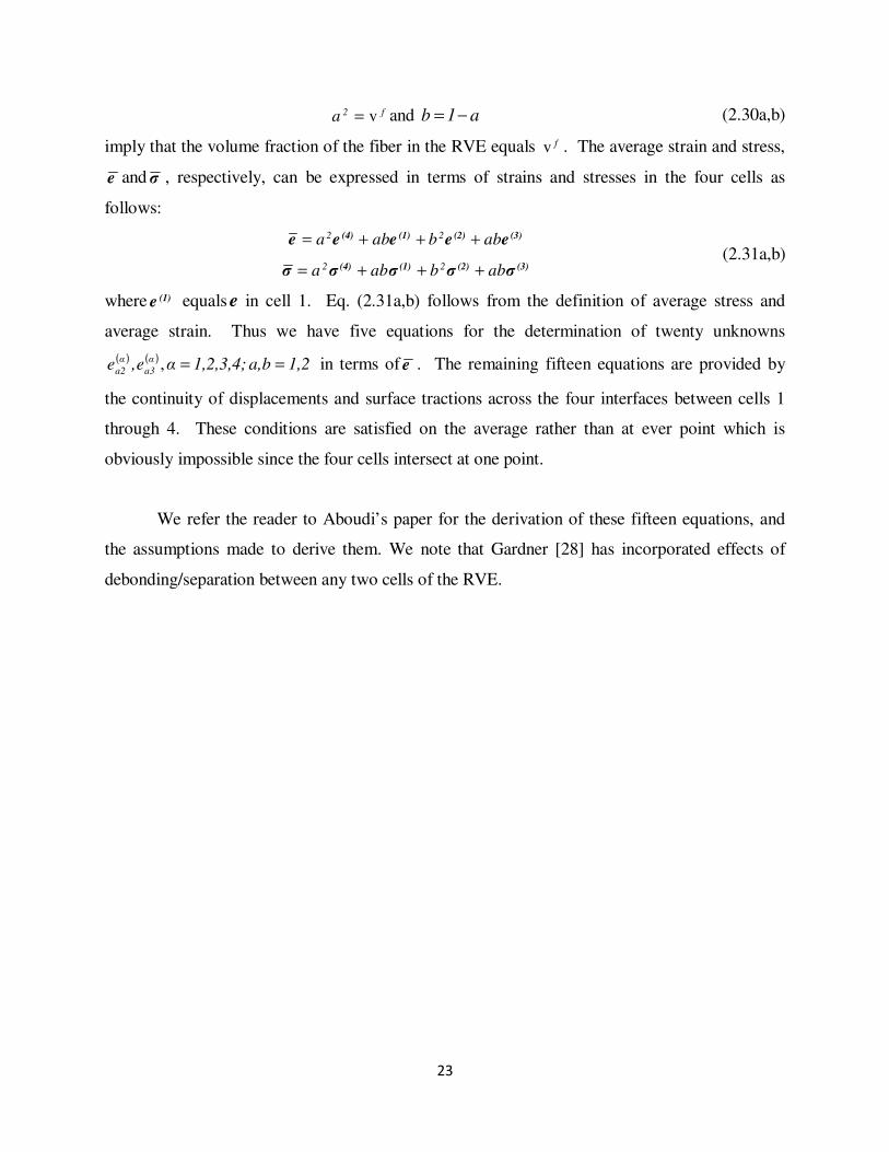
f2a v= and a1b −= (2.30a,b)
imply that the volume fraction of the fiber in the RVE equals fv . The average strain and stress,
e andσ , respectively, can be expressed in terms of strains and stresses in the four cells as
follows:
(3)(2)(1)(4) eeeee abb ab a 22 +++=
(3)(2)(1)(4)σσσσσ abb ab a 22 +++=
(2.31a,b)
where (1)e equals e in cell 1. Eq. (2.31a,b) follows from the definition of average stress and
average strain. Thus we have five equations for the determination of twenty unknowns
( ) ( ) 1,2ba,1,2,3,4;αe,e α
a3
α
a2==, in terms of e . The remaining fifteen equations are provided by
the continuity of displacements and surface tractions across the four interfaces between cells 1
through 4. These conditions are satisfied on the average rather than at ever point which is
obviously impossible since the four cells intersect at one point.
We refer the reader to Aboudi’s paper for the derivation of these fifteen equations, and
the assumptions made to derive them. We note that Gardner [28] has incorporated effects of
debonding/separation between any two cells of the RVE.
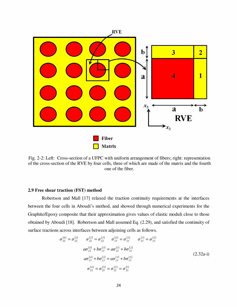
24
Fig. 2-2: Left: Cross-section of a UFPC with uniform arrangement of fibers; right: representation of the cross-section of the RVE by four cells, three of which are made of the matrix and the fourth
one of the fiber.
2.9 Free shear traction (FST) method
Robertson and Mall [17] relaxed the traction continuity requirements at the interfaces
between the four cells in Aboudi’s method, and showed through numerical experiments for the
Graphite/Epoxy composite that their approximation gives values of elastic moduli close to those
obtained by Aboudi [18]. Robertson and Mall assumed Eq. (2.29), and satisfied the continuity of
surface tractions across interfaces between adjoining cells as follows.
( ) ( )1
22
4
22 σσ = ( ) ( )3
22
2
22 σσ =
( ) ( )3
33
4
33σσ =
( ) ( )2
33
1
33σσ =
( ) ( ) ( ) ( )2
12
1
12
3
12
4
12 bσaσbσaσ +=+
( ) ( ) ( ) ( )2
13
3
13
1
13
4
13bσaσbσaσ +=+
( ) ( ) ( ) ( )1
23
2
23
3
23
4
23 σσσσ ===
(2.32a-i)

25
Eq. (2.32a-d) imply the continuity of normal tractions across interfaces perpendicular to the -x2
and the -x3 axes. Eqs. (2.32e) and (2.32f) follow from the requirement that the total tangential
force in the -x1 direction on the planes =2x constant and =3x constant are continuous. Eq.
(2.32g-i) states that the shear stress 23σ has the same constant value in the four cells. It is clear
that the continuity of tangential tractions 23σ is being satisfied in a way different from the
continuity of tangential tractions 12σ and 13σ . In order that the four cells do not separate from
each other during any deformation Robertson and Mall [17] imposed the following requirements
on the uniform strains in the four cells.
( ) ( ) ( ) ( ) ( ) 222
22
3
22
1
22
4
22 ebabeaebeae +=+=+
( ) ( ) ( ) ( ) ( ) 332
33
1
33
3
33
4
33 ebabeaebeae +=+=+
( ) ( )3
12
4
12 ee = ( ) ( )2
12
1
12 ee =
( ) ( ) ( ) 121
12
4
12 ebabeae +=+
( ) ( )1
13
4
13ee = ( ) ( )3
13
2
13ee =
( ) ( ) ( ) 133
13
4
13 ebabeae +=+
( ) ( ) ( ) ( ) ( )( ) 233
23
2
2321
23
4
232 ebabaabeebabeea ++=+++
(2.33a-k)
Eq. (2.33a-d) reflects the requirement that the total displacement of the RVE in the -x2 and the
-x3 directions equals the sum of the displacements of cells in those directions. In order to
motivate Eq. (2.33e-j) we assume that 0u1 = . Eq. (2.33e,f,i) implies that during the shear
deformation given by 12e , the average -x2 displacement across the interface between cells 4 and
3, and that between cells 1 and 2 are the same. Furthermore, the sum of the -x2 displacement of
the interface between cells 4 and 3, and that between cells 1 and 3 equals the average
displacement of the RVE in the -x2 direction. Eq. (2.33k) is the same as Eq. (2.31a) for 23e .We
note that Eq. (2.31a) is satisfied for other components of e when Eq. (2.33b-k) holds.
We substitute for stresses in Eq. (2.32) from Eqs. (2.1) and (2.5) in terms of the elastic
moduli of the fiber and the matrix and strains in the four cells, and obtain 24 linear equations for
determining the twenty four unknowns (3)(2)(1) eee ,, and (4)e in terms of six components of e .

26
Said differently, we can find strain concentration tensors for (3)(2)(1) eee ,, and (4)e . Thus the strain
concentration tensors depend upon the elastic moduli of the matrix and the fiber, and the volume
fraction of fibers but not on the shape and the distribution of fibers.
3. Elasto-plastic material parameters
3.1 Preliminaries
The polymer in a UFPC usually exhibits an elasto-plastic response. However, fibers
deform elastically and are brittle. Consequently, the failure strain of a UFPC in the direction of
fibers is small and one can neglect effects of geometric nonlinearities. We first briefly review
elasto-plastic deformations of the polymer and the UFPC and then using the FST approach
determine parameters that appear in the plastic potential as well as find the functional
dependence of effective stress on effective plastic strain of a UFPC .
We note that yielding of polymers may not be independent of the hydrostatic pressure as
it is for most metals. For polycarbonates and polymethylmetharcylates the yield stress is known
to depend upon the hydrostatic pressure p. Pressure-dependent yield functions have been
discussed by Caddell et al. [13], and Hu and Pae [14].
3.2 Infinitesimal elasto-plastic deformations of polymer
3.2.1 Pressure independent yielding of polymer
We employ an incremental theory of plasticity and assume that during an incremental
deformation, the increment, ed , in the strain has an additive decomposition into elastic, eed , and
plastic, ped , strains. That is
peeee ddd += (3.1)
Eq.(2.1) relates the corresponding incremental stress, σd , with the incremental elastic strain eed .
For relating pde to σd , we assume the von Mises plastic potential for the polymer, i.e.,
( ) ( ) ( ) ( ) 212
213
223
2
2211
2
1133
2
3322ij 2σ2σ2σσσ3
1σσ
3
1σσ
3
1σ2F +++−+−+−= (3.2)

27
Here we have expressed the plastic potential in terms of σ rather than in terms of the deviatoric
stressijkkijij δσ
3
1σs −= . In Eq. (3.2) we have tacitly assumed that the polymeric response is
isotropic.
We use the associated flow rule for relating ped to σd , i.e.,
ij
pij
σ
Fdλde
∂
∂= (3.3)
where dλ is the proportionality factor. Eq. (3.3) implies that pde is normal to the yield surface
( ) mij
σσF =
(3.4)
where mσ3 is the yield stress of the polymer in a simple tension or compression test.
We define the effective stress σ by
( )ijσ3Fσ = (3.5)
and the effective plastic strain, pe , by requiring that in any incremental deformation,
pij
p
ij edσσde = (3.6)
We note that mσσ = in a uniaxial tension or compression test. Substituting for p
ijde in Eq. (3.6)
from Eq. (3.3) and using Eq. (3.5) we get
σ
σd
2H
3
σ
ed
2
3dλ
m
p
== (3.7)
where the strain-hardening modulus,
p
m
ed
σdH = , has been assumed to be positive. The function
( )pm eH is found from experimental data.
Taking the differential on both sides of Eq. (3.5) we get
ijijkk
ij dσδ3
σσ
σ2
3σd
−= (3.8)
Substituting fordλ from Eq. (3.7) and for σd from Eq. (3.8) into Eq. (3.3) we get

28
kl
mp
ijklpqpq
ll
pqij
kk
ij2m
p
ij dσSdσδ3
σσ
σσ
σ4H
9de =
−
−
= δ
3 (3.9)
where mpS is the plastic compliance matrix of the polymer.
Expressing strain increments on the right-hand side of Eq. (3.1) in terms of incremental
stress we get
σSσSe mpme ddd += (3.10)
where ( )m−
=1
meS C is the elastic compliance matrix for the polymer. Hence
( ) eSSσmpme dd
1−+= (3.11)
which expresses incremental stresses in terms of incremental strains. We note that mpS depends
upon current values of σ , and normal stresses may affect ensuing shear strains.
The dependence of the flow stress, mσ , in Eq. (3.4) upon the effective plastic strain, pe ,
is determined from the test data. It will also determine mH .
3.2.2 Pressure-dependent yielding of polymer
To account for the pressure sensitive yielding of polymers, the Drucker-Prager yield
potential is used, and the effective stress is taken to be
kkmα3Fσ σ+= (3.12a)
where the parameter mα accounts for hydrostatic effects. The Drucker-Prager yield surface is
given by
mkk
m βσα3F =+ (3.12b)
where mβ is a material parameter.
Values of parameters mα and mβ can be found from the magnitudes of the yield stresses
tyσ and c
yσ in simple tension and compression tests. That is
mcy
mcy
ty
mty βσασσασ =−=+ (3.12c)
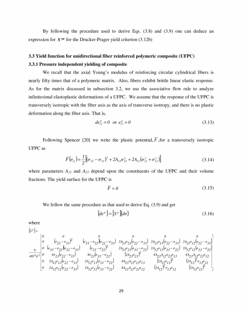
29
By following the procedure used to derive Eqs. (3.8) and (3.9) one can deduce an
expression for mpS for the Drucker-Prager yield criterion (3.12b)
3.3 Yield function for unidirectional fiber reinforced polymeric composite (UFPC)
3.3.1 Pressure independent yielding of composite
We recall that the axial Young’s modulus of reinforcing circular cylindrical fibers is
nearly fifty times that of a polymeric matrix. Also, fibers exhibit brittle linear elastic response.
As for the matrix discussed in subsection 3.2, we use the associative flow rule to analyze
infinitesimal elastoplastic deformations of a UFPC. We assume that the response of the UFPC is
transversely isotropic with the fiber axis as the axis of transverse isotropy, and there is no plastic
deformation along the fiber axis. That is,
0de p
11 = or 0e p11 = (3.13)
Following Spencer [20] we write the plastic potential, F ,for a transversely isotropic
UFPC as
( ) ( ) ( )[ ]212
21312
22323
2
3322ij σσ2Aσ2Aσσ2
1σF +++−= (3.14)
where parameters A12 and A23 depend upon the constituents of the UFPC and their volume
fractions. The yield surface for the UFPC is
σF = (3.15)
We follow the same procedure as that used to derive Eq. (3.9) and get
[ ] dσSde pp = (3.16)
where
[ ]
( ) ( )( ) ( ) ( ) ( )( )( ) ( ) ( ) ( ) ( )
( ) ( ) ( )( ) ( ) ( ) ( )( ) ( ) ( ) ( )
−−
−−
−−
−−−−−−
−−−−−−
=
212σ
122A
12σ
13σ
212
2A12σ
23σ
12A
234A
22σ
33σ
12σ
122A
33σ
22σ
12σ
122A0
12σ
13σ
212
2A2
13σ
122A
13σ
23σ
12A
234A
22σ
33σ
13σ
122A
33σ
22σ
13σ
122A0
12σ
23σ
12A
234A
13σ
23σ
12A
234A
223σ
232A
22σ
33σ
234σ
33σ
22σ
234σ0
22σ
33σ
12σ
122A
22σ
33σ
13σ
122A
22σ
33σ
23σ
232A
222σ
33σ
33σ
22σ
22σ
33σ0
33σ
22σ
12σ
122A
33σ
22σ
13σ
122A
33σ
22σ
23σ
232A
33σ
22σ
22σ
33σ
233σ
22σ0
000000
σ4H
9
S
2p
p

30
pH equals the strain hardening modulus of the UFPC, and the stress and the strain increments
are written in the Voigt notation.
Knowing the elastic compliance matrix, S , for the composite obtained from the micro-
mechanics theories discussed in section 2 we can determine the elastic-plastic compliance matrix
( )pSS + .
3.3.2 Pressure dependent yielding of composite
To account for the pressure sensitive yielding of composites, the Drucker-Prager yield
potential for the composite is adopted, and the effective stress is defined as
( )3322 σσαF3σ ++= (3.17)
where the parameter α accounts for effects of the hydrostatic pressure on the yielding of the
UFPC. The term ( )3322 σσα + in Eq. (3.21) does not contain 11σ because of the assumption 0e p11 =
for the UFPC. One can derive the elastic-plastic compliance matrix for this case by following
the same procedure as that outlined above.
3.4 Determination of elastic-plastic parameters of the UFPC
3.4.1 Pressure-independent yield surface
We use the FST [17] method to compute the effective stress versus the effective plastic
strain curve for the UFPC from a knowledge of the material properties of the constituents of the
UFPC and the volume fraction of fibers. One way to obtain this curve is to study plane stress
deformations of a thin lamina with the fiber axis making an angle θ counter clockwise with the
−x axis of loading as shown in Fig 2-3. Thus with respect to the global rectangular Cartesian
coordinate axes ( )zy,x, , the only non-zero component of the stress tensor is xxσ .

31
Fig. 2-3: Fiber orientation with respect to the axis of loading, and the material principal axes
( )321 x,x,x .
Using either the Mohr circle or the stress transformation equations, stresses with respect
to the material principal axes ( )321 x,x,x are given by
θoscσσ 2xx11 = , θsinσσ 2
xx22= and θ cos θ sinσσ xx12 −= (3.18)
Substituting for stresses from Eq. (3.18) into Eq. (3.2), and the result into Eq. (3.5) we get
[ ] xx2
122
12
4 σθθcossin2Aθsin2
3σ += (3.19)
It follows from Eq. (3.6) that
xx
p
xx
p σdeedσ = (3.20)
and therefore
[ ] 21
22
12
4
p
xxp
θθcossin2Aθsin2
3
deed
+
= (3.21)
Thus
[ ] 21
22
12
4
xx
xxxx
p
θθcossin2Aθsin2
3
Eσ
-e
e
+
= (3.22)
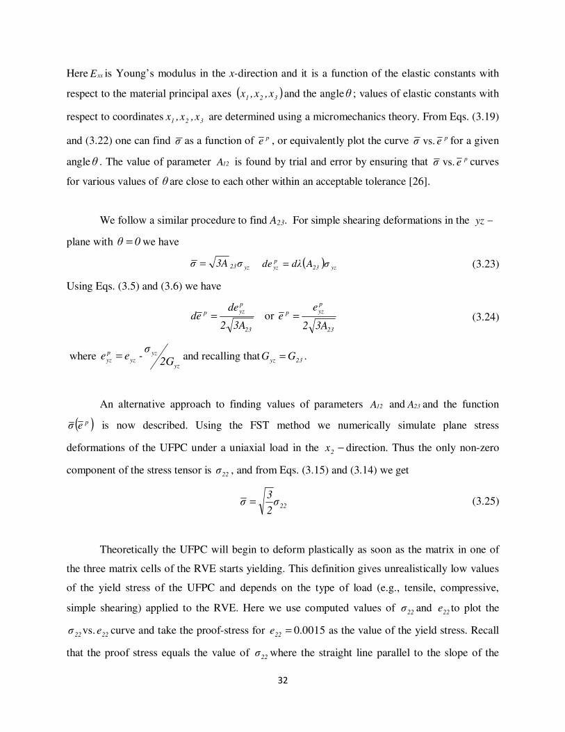
32
Here xxE is Young’s modulus in the x-direction and it is a function of the elastic constants with
respect to the material principal axes ( )321 x,x,x and the angleθ ; values of elastic constants with
respect to coordinates 321 x,x,x are determined using a micromechanics theory. From Eqs. (3.19)
and (3.22) one can find σ as a function of pe , or equivalently plot the curve pe σ vs. for a given
angleθ . The value of parameter 12A is found by trial and error by ensuring that pe σ vs. curves
for various values of θ are close to each other within an acceptable tolerance [26].
We follow a similar procedure to find A23. For simple shearing deformations in the −yz
plane with 0θ = we have
yz23σ3Aσ = ( ) yz23pyz σAdλde = (3.23)
Using Eqs. (3.5) and (3.6) we have
23
pyzp
3A2
deed = or
23
p
yzp
3A2
ee = (3.24)
where yz
yzyz
p
yz 2G
σ-ee = and recalling that
23yzGG = .
An alternative approach to finding values of parameters 12A and 23A and the function
( )peσ is now described. Using the FST method we numerically simulate plane stress
deformations of the UFPC under a uniaxial load in the −2x direction. Thus the only non-zero
component of the stress tensor is 22σ , and from Eqs. (3.15) and (3.14) we get
22σ2
3σ = (3.25)
Theoretically the UFPC will begin to deform plastically as soon as the matrix in one of
the three matrix cells of the RVE starts yielding. This definition gives unrealistically low values
of the yield stress of the UFPC and depends on the type of load (e.g., tensile, compressive,
simple shearing) applied to the RVE. Here we use computed values of 22σ and 22e to plot the
2222 eσ vs. curve and take the proof-stress for 0015.0=22e as the value of the yield stress. Recall
that the proof stress equals the value of 22σ where the straight line parallel to the slope of the

33
2222 eσ vs. curve at 0=22e (Young's modulus at zero strain) passing through the point
( )0015.00 == 2222 e ,σ intersects the 2222 eσ vs. curve. We thus find yieldσ when the UFPC begins
to yield as
PS
22yield σ2
3σ = (3.26)
where PS
22σ equals the proof-stress 22σ .
In order to find values of 12A and 23A we use the FST technique to simulate simple
shearing deformations of the UFPC in the −21xx and the −32 xx planes. Using the same
definition of the yield stress as that adopted in Eq. (3.26) we obtain
PS
2323
PS
1212yield σ3Aσ3Aσ == (3.27a,b)
We find yieldσ from Eq. (3.26), and then values of parameters 12A and 23A from Eq. (3.27a,b).
We note that in Weeks and Sun's [26] approach values of parameters 12A , 23A and yieldσ
are determined by considering pe σ vs. curves for the entire range of values of pe considered,
and σσyield
= when 0=pe . Thus the value of yieldσ is determined after values of 12A and 23A
have been found. The ( )peσ function is found from the computed pe σ vs. curve by the least
squares method. However, in the alternative approach proposed here values of 12A , 23A and yieldσ
are found from those of the proof stresses in uniaxial loading in the transverse direction, and in
simple shearing deformations in the −21xx and the −32 xx planes.
3.4.2 Pressure-dependent yield surface
We now need to find values of parameters α , 12A , 23A and yieldσ . When using Weeks and
Sun's [26] approach we find values of αand 12A by ensuring that the pe σ vs. curves for different
values of the fiber-orientation θ in Fig. 2-3 and positive and negative values of xxσ are close to
each other within the prescribed tolerance. Subsequently, the value of 23A is chosen so that the
pe σ vs. curve for the simple shearing deformations in the −yz plane is close to the pe σ vs.
curve for uniaxial loading.
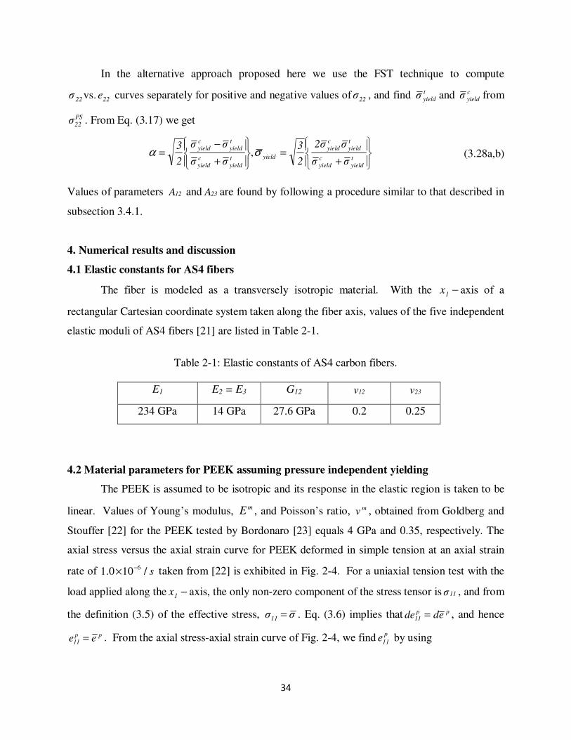
34
In the alternative approach proposed here we use the FST technique to compute
2222 eσ vs. curves separately for positive and negative values of 22σ , and find tyieldσ and c
yieldσ from
PS
22σ . From Eq. (3.17) we get
+=
+
−=
tyield
cyield
tyield
cyield
yieldtyield
cyield
tyield
cyield
σσ
σσ2
2
3
σσ
σσ
2
3σα ,
(3.28a,b)
Values of parameters 12A and 23A are found by following a procedure similar to that described in
subsection 3.4.1.
4. Numerical results and discussion
4.1 Elastic constants for AS4 fibers
The fiber is modeled as a transversely isotropic material. With the −1x axis of a
rectangular Cartesian coordinate system taken along the fiber axis, values of the five independent
elastic moduli of AS4 fibers [21] are listed in Table 2-1.
Table 2-1: Elastic constants of AS4 carbon fibers.
E1 E2 = E3 G12 12ν 23ν
234 GPa 14 GPa 27.6 GPa 0.2 0.25
4.2 Material parameters for PEEK assuming pressure independent yielding
The PEEK is assumed to be isotropic and its response in the elastic region is taken to be
linear. Values of Young’s modulus, mE , and Poisson’s ratio, mν , obtained from Goldberg and
Stouffer [22] for the PEEK tested by Bordonaro [23] equals 4 GPa and 0.35, respectively. The
axial stress versus the axial strain curve for PEEK deformed in simple tension at an axial strain
rate of 61.0 10 / s
−× taken from [22] is exhibited in Fig. 2-4. For a uniaxial tension test with the
load applied along the −1x axis, the only non-zero component of the stress tensor is 11σ , and from
the definition (3.5) of the effective stress, σσ11 = . Eq. (3.6) implies that pp11 edde = , and hence
pp11 ee = . From the axial stress-axial strain curve of Fig. 2-4, we find p
11e by using

35
E
σee 11
11
p
11 −= (4.1)
and plot the pe σ vs. curve shown in Fig. 2-5 where it has been tacitly assumed that the yield
stress of PEEK in uniaxial tension and compression equals 40 MPa. Assuming that σ and pe are
related by
−=
N
Aσxpee p (4.2)
in the range 40MPaσ94MPa ≥≥ , values of A and N found by the least squares method and
having a regression coefficient of 0.986 are MPa152.7A = and MPa13.86N =
Fig. 2-4: Computed and experimental axial stress vs. axial strain curves for PEEK polymer.
0
25
50
75
100
0 0.01 0.02 0.03 0.04 0.05
Axia
l st
ress
(M
Pa)
Axial strain
Current numerical analysis
Expt. [23]
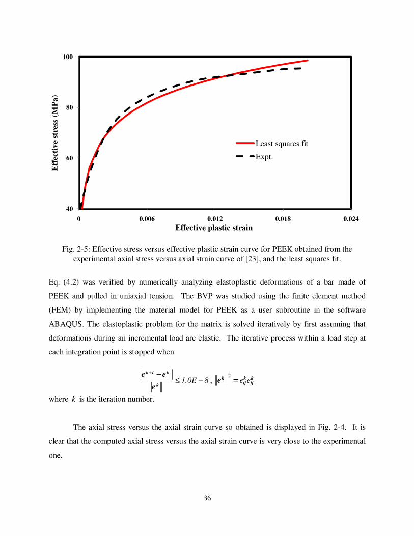
36
Fig. 2-5: Effective stress versus effective plastic strain curve for PEEK obtained from the
experimental axial stress versus axial strain curve of [23], and the least squares fit.
Eq. (4.2) was verified by numerically analyzing elastoplastic deformations of a bar made of
PEEK and pulled in uniaxial tension. The BVP was studied using the finite element method
(FEM) by implementing the material model for PEEK as a user subroutine in the software
ABAQUS. The elastoplastic problem for the matrix is solved iteratively by first assuming that
deformations during an incremental load are elastic. The iterative process within a load step at
each integration point is stopped when
81.0E −≤−+
k
k1k
e
ee, k
ijkij
ke ee=2
where k is the iteration number.
The axial stress versus the axial strain curve so obtained is displayed in Fig. 2-4. It is
clear that the computed axial stress versus the axial strain curve is very close to the experimental
one.
40
60
80
100
0 0.006 0.012 0.018 0.024
Eff
ecti
ve
stre
ss (
MP
a)
Effective plastic strain
Least squares fit
Expt.

37
4.3 Material parameters for PEEK assuming pressure dependent yielding
Zheng's [27] experimental uniaxial tension and compression stress strain curves for
PEEK at strain rates of 1.0E-6/s and 1.0E-5/s, respectively, are shown in Fig. 2-6. From Eq.
(3.12a) for uniaxial tension test, the effective stress σ and the effective plastic strain pe can be
expressed in terms of the axial stress 11σ and the axial plastic strain p
11e , that is,
( ) 11
m σα1σ += and ( ) ( )m
m
1111
m
p
11p
α1
E
σe
α1
ee
+
−=
+=
(4.3)
Similarly, for uniaxial compression we have
( ) 11m σα1σ −= and
( )m
m
11
11p
α1
E
σe
e−
−=
(4.4)
From the experimental uniaxial stress strain curves for tension and compression tests, the
effective stress and the effective plastic strains can be evaluated using Eqs. (4.3) and (4.4). The
value of mα is chosen so that the effective stress versus effective plastic strain curves for both
tension and compression tests overlap within an acceptable tolerance. Fourth order polynomials
were fit to the effective stress versus effective plastic strain curves for tension and compression
data and the percentage difference was found using
( )
( )100
σ
σσ
e%Differenc
i
2t
i
i
2c
i
t
i
∑
∑ −
= (4.5)
where t
iσ and c
iσ are the effective stress values from tension and compression tests, respectively,
corresponding to the effective plastic strain p
ie . The entire range of pe was divided into 30 equal
segments and values at the mid-point of a segment were used in Eq. (4.5).
Fig. 2-7 shows the effective stress versus the effective plastic strain curve for uniaxial
compression and tension tests obtained from Zheng [27]. Also shown in Fig. 2-7 is the least
squares curve fit for 0.1645=mα . The difference between the effective stress versus effective
plastic strain curves from tension and compression data using Eq. (4.5) was found to be 1.7% for
effective plastic strain up to 3.0%.

38
The value of mα was also determined using the value of the proof stress at yield from
uniaxial compression and tension tests. The expression for mα in terms of the proof stress in
tension,
PS
tσ , and compression, PS
cσ , obtained from Eqs. (4.3) and (4.4) is
+
−=
PSt
PSc
PS
t
PS
cm
σσ
σσα
(4.6)
From the experimental curves depicted in Fig. 2-6, we found that 57MPa=PS
tσ and
MPa37=PS
cσ . Substituting for PS
tσ and PS
cσ in the expression for mα in Eq. (4.6), we get
0.123=mα . The difference between the effective stress versus effective plastic strain curves
from tension and compression data using Eq. (4.5) was found to be 16.6% for effective plastic
strain of up to 3.0%. As mentioned earlier Weeks and Sun's [26] approach uses the entire set of
data for 0.030 ≤≤ pe whereas the present approach uses values of proof stresses which vary with
the definition of the proof stress. For example, one could define the proof stress as the stress
corresponding to the strain of 1.3% rather than 1.5%.
For the relation (4.2) values of A and N obtained by the least squares method with a
regression coefficient of 0.954 and 0.1645=mα are 144.0 MPa and 8.69 MPa, respectively. In
Fig. 2-6 we have compared the experimental uniaxial stress strain curves with the curves
obtained from implementing the material model for PEEK as a user subroutine in ABAQUS and
employing the above listed values of mα , A and N. It is evident that the computed axial stress
versus the axial strain curves are close to the experimental ones.

39
Fig. 2-6: Comparison of computed and experimental axial stress vs. axial strain curves for PEEK
polymer deformed in uniaxial tension and compression.
Fig. 2-7: Effective stress versus effective plastic strain curve for PEEK obtained from the
experimental axial stress versus axial strain curve of [27].
0
40
80
120
0 0.02 0.04 0.06
Axia
l st
ress
(M
Pa
)
Axial strain
Expt. tension [27]
Current analysis, tension
Expt. compression [27]
Current analysis, compression
60
80
100
120
0 0.01 0.02 0.03 0.04 0.05
Eff
ecti
ve
stre
ss (
MP
a)
Effective plastic strain
Compression
Tension
Least squares fit
40
4.4 Elastic parameters of the composite
When using Hill’s theorem, we note that it is simpler to adopt the following approach
than to use Eq. (2.12). For the displacement field joiji xeu = imposed on the boundaries of the
RVE, we equate the work done by external forces on the homogenized RVE to that on the
composite RVE. That is,
∫∫ ==Γ
joiji
Γ
iioij
oij dsxef
Ω
1dsuf
Ω
1σe
(4.7a)
where fi is the surface traction on the boundaries of the composite RVE. Since Eq. (4.7a) must
hold for all values of o
ije , therefore
∑∫ == ji
Γ
jioij xR
Ω
1dsxf
Ω
1σ
(4.7b)
where dsfR ii = is the reaction force and Γ is the boundary surface of the RVE. The RVE,
depicted in Fig. 2-8, consists of nine uniformly distributed fibers in the matrix. The linear elastic
BVP for the composite RVE under displacement boundary conditions joiji xeu = is numerically
solved using the commercial software ABAQUS, and reaction forces iR at the boundary surfaces
are found. The deformed configurations depicted in Fig. 2-8 of the RVE are for tensile
deformations along the -x1
axis obtained by prescribing ,0,0xeu 1011= on the boundary and for
pure shear deformations in the -xx21
plane obtained by assigning displacements
,0xe,xeu 1
0
122
0
12= on the bounding surfaces of the RVE. We note that for ,0,0xeu 1
011= the
specimen is not deformed in uniaxial tension since the other two components of displacements
are constrained to be zero. From the deformed configuration depicted in Fig. 2-8, it is evident
that small matrix regions surrounding the fibers are more intensely deformed than the remainder
of the matrix. For each of the six displacement boundary conditions involving ,011e , 0
22e , 0
33e , 0
12e ,
0
13e
and
0
23e the stress vector 0
12013
023
033
022
011 σ,σ,σ,σ,σ,σ
is calculated using Eq. (4.7b) from which
ijklC is obtained.

41
Fig. 2-8: Cross-sections of cubic RVEs with fibers parallel to the -x3
axis; (top): undeformed
configuration, (bottom left) and (bottom right): configurations obtained by applying
displacement fields ,0,0xeu 1
0
11= and ,0xe,xeu 1
0
122
0
12= , respectively, to the boundaries.
Robertson and Mall [17] have shown that their FST method gives results close to those
derived from Aboudi’s [6] method of cells. Consequently, we did not compute results from
Aboudi’s method.
For each one of the micromechanical theories studied here values of Young’s modulus
1E essentially follow the rule of mixtures and are not plotted here.
We have plotted in Figs. 2-9 through 2-13 values of E2, G12, G23, 12ν and 23ν as a
function of the volume fraction, fv , of the fibers. In general, the curves exhibited in Figs. 2-9

42
through 2-13 are not straight lines. Even for 0.3v =f different micromechanics approaches do
not give the same value of an elastic modulus.
For 0.6v =f , the experimentally determined values of E2 = E3, G12 = G13, G23, ν12 and
ν23 are exhibited in these figures. Except for possibly different curing methods, it is unclear why
various experimentalists obtained different values of these elastic constants. The difference
between the minimum and the maximum values of E2, G12, ν12 and ν23 equals 11, 11, 16, and 4%,
respectively.
Out of the four micromechanics approaches adopted here, Hill’s and the FST methods
give not only values of E2 that are close to each other but these values are also close to the test
data. Eshelby’s equivalent inclusion and the Mori-Tanaka techniques noticeably underestimate
values of E2. We did not compute results for 0.3v <f since for most composites applications
0.3v >f .
For a given volume fraction of the fibers, the value of G12 computed by Hill’s method is
considerably more than that estimated by using the other three approaches, and it also far
exceeds the experimentally found value. This is possibly due to the strain concentrations around
nearly rigid fibers. An examination of fringe plots of stresses showed that equal and opposite
stresses were developed near the North and South poles of fibers that equilibrated each other but
contributed to the energy required to deform the fibers. Also for the simple shearing
deformations, local values of strain components other than e12 were non-zero even though their
average values were null.
For 0.3,v =f the micromechanics theories provide values of G23 that are reasonably
close to each other. Hill’s method in this case yields good values of G23 for the composite
because G23 for the fiber is less than four times that of the matrix, and there are fewer places of
strain concentrations. The Mori-Tanaka method and Hill’s equivalent energy principle provide
values of G23 that are close to each other. We note that the differences in the values of G23
increase with an increase in the volume fractions of fibers. For this case the FST and the EIM
severely underestimate values of G23.

43
For 0.6v =f the micromechanics theories that provide good values of E2, G12 and G23
do not yield values of ν12 and ν23 that are close to the test data. For 0.3,v =f the four
micromechanics approaches give close values of ν12 but not of ν23.
It is clear from the plots exhibited in Fig. 2-13 that values of 23ν do not obey the rule of
mixtures since 23ν for 0.3v =f is greater than the value of Poisson’s ratio for the matrix.
Furthermore, the rule of mixtures implies that an elastic modulus is an affine function of .v f
The foregoing observations of the computed values of the elastic moduli suggest that
none of the four micromechanics approaches provides values of the five elastic moduli that are
very close to the corresponding experimentally found values.
Fig. 2-9: Variation with fv of the elastic modulus E2 = E3 obtained using different
micromechanics approaches; M-T = Mori-Tanaka, FST = free shear traction, EIM = Eshelby’s
inclusion method.
4
6
8
10
12
0.2 0.4 0.6 0.8
Ela
stic
mod
ulu
s, E
2=
E3
(GP
a)
Fiber volume fraction
M-T
FST
EIM
Hill's method
Expt.[24]
Expt.[25]
Expt.[26]

44
Fig. 2-10: Variation with fv of the elastic modulus G12 = G13 obtained using different
micromechanics approaches; M-T = Mori-Tanaka, FST = free shear traction, EIM = Eshelby’s
inclusion method.
Fig. 2-11: Variation with fv of the elastic modulus G23 obtained using different micromechanics
approaches; M-T = Mori-Tanaka, FST = free shear traction, EIM = Eshelby’s inclusion method.
2
4
6
8
0.2 0.4 0.6 0.8
Sh
ea
r m
od
ulu
s, G
12
=G
13
(GP
a)
Fiber volume fraction
M-T
FST
EIM
Hill's method
Expt.[24]
Expt.[25]
Expt.[26]
1
2
3
4
0.2 0.4 0.6 0.8
Sh
ear m
od
ulu
s, G
23
(GP
a)
Fiber volume fraction
M-T
FST
EIM
Hill's method
Expt.[26]

45
Fig. 2-12: Variation with fv of the Poisson’s ratio 12ν
obtained using different micromechanics
approaches; M-T = Mori-Tanaka, FST = free shear traction, EIM = Eshelby’s inclusion method.
Fig. 2-13: Variation with fv of the Poisson’s ratio 23ν obtained using different micromechanics
approaches; M-T = Mori-Tanaka, FST = free shear traction, EIM = Eshelby’s inclusion method.
0.2
0.25
0.3
0.35
0.2 0.4 0.6 0.8
Pois
son
's r
ati
o, νν νν
12
Fiber volume fraction
M-T
FST
EIM
Hill's method
Expt.[24]
Expt. [26]
0.25
0.3
0.35
0.4
0.45
0.5
0.2 0.4 0.6 0.8
Pois
son
's r
ati
o, νν νν
23
Fiber volume fraction
M-T
FST
EIM
Hill's method
Expt.[24]
Expt. [26]

46
4.5 Elasto-plastic properties of the composite
4.5.1 Validity of the FST approach for elasto-plastic deformations
Given values of elastic moduli of the fiber and the matrix, and the effective stress, σ , of
the matrix as a function of the effective plastic strain, pme , for the matrix, we find values of 12A ,
23A and ( )peσ for the UFPC. A user defined subroutine based on the FST method of subsection
2.8 has been implemented in the FE software, ABAQUS. The three matrix cells deform elasto-
plastically and the fiber cell elastically.
In order to determine the elastoplastic material response of the AS4/PEEK composite
two material models for the polymer are considered; one assumes that the hydrostatic pressure
contributes to plastic deformations [27] (discussed in subsection 3.2.2) and the other assumes the
von Mises yield surface in which plastic deformations are independent of the hydrostatic
pressure [24] (discussed in subsection 3.2.1). The elastic-plastic properties for pressure
insensitive and pressure sensitive polymer are given in subsections 4.2 and 4.3, respectively.
Using material properties of the constituents and the volume fraction of fibers we simulated
uniaxial deformations of the composite. Since the specimen is expected to deform
homogeneously only one FE is used to simulate these tests.
For ,6.0v =f Figs. 2-14, 2-15 and 2-16 compare the computed axial stress versus the
axial strain curves for off-axis loading (e.g. see Fig. 2-3) with experimental results reported by
Weeks and Sun [26]. It is clear that the axial stress versus the axial strain response obtained
using the pressure independent von Mises yield surface for the polymer is in better agreement
with the experimental data than that when the polymer is modeled with the pressure dependent
Drucker-Prager yield surface.
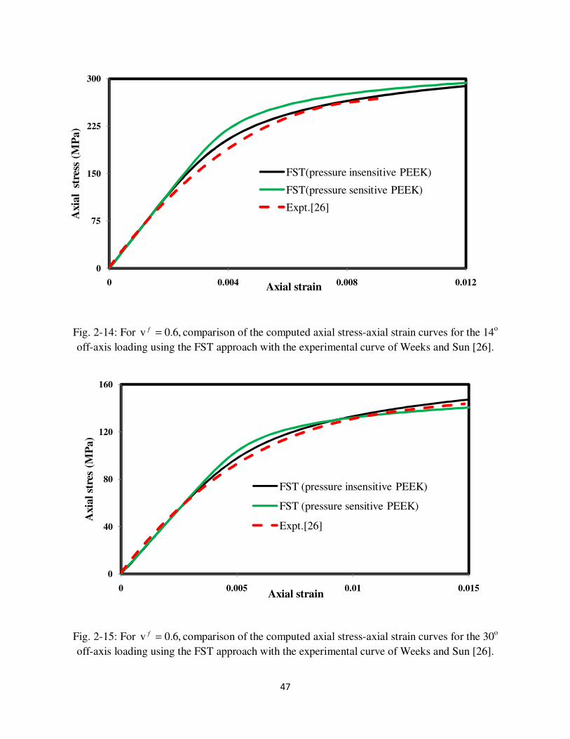
47
Fig. 2-14: For ,6.0v =f comparison of the computed axial stress-axial strain curves for the 14o
off-axis loading using the FST approach with the experimental curve of Weeks and Sun [26].
Fig. 2-15: For ,6.0v =f comparison of the computed axial stress-axial strain curves for the 30o
off-axis loading using the FST approach with the experimental curve of Weeks and Sun [26].
0
75
150
225
300
0 0.004 0.008 0.012
Axia
l s
tres
s (M
Pa)
Axial strain
FST(pressure insensitive PEEK)
FST(pressure sensitive PEEK)
Expt.[26]
0
40
80
120
160
0 0.005 0.01 0.015
Axia
l st
res
(MP
a)
Axial strain
FST (pressure insensitive PEEK)
FST (pressure sensitive PEEK)
Expt.[26]

48
Fig. 2-16: For ,6.0v =f comparison of the computed axial stress-axial strain curves for the 45o
off-axis loading using the FST approach with the experimental curve of Weeks and Sun [26].
4.5.2 Values of material parameters for the homogenized composite
Values of material parameters appearing in the yield surfaces of the UFPC are
determined from the FST method. For ,6.0v =f and using the techniques discussed in
subsection 3.4, we get
(a) Pressure independent yield surface
(i) Weeks and Sun's approach
A12 = 7.5 A23 = 8.5 A = 496.6 MPa N = 35.2 MPa
(ii) Present approach
A12 = 5.45 A23 = 6.47 A = 388.5 MPa N = 24.4 MPa
0
30
60
90
120
0 0.005 0.01 0.015
Axia
l st
ress
(M
Pa
)
Axial strain
FST(pressure insensitive PEEK)
FST(pressure sensitive PEEK)
Expt.[26]

49
(b) Pressure dependent yield surface 0.544α =
(i) Weeks and Sun's approach
A12 = 2.1 A23 = 2.2 A = 250.0 MPa N = 15.4 MPa
(ii) Present approach
A12 = 3.22 A23 = 3.47 A = 303.7 MPa N = 16.7 MPa
4.5.3 Comparison of results from the FST method with those from the homogenized
composite
Figs. 2-17, 2-18 and 2-19 compare the axial stress versus the axial strain curves for off-
axis loading obtained from the FST method with the axial stress versus the axial strain response
for the pressure insensitive yielding of composites using above-listed values of material
parameters determined. It is clear that the three sets of curves are close to each other.
Fig. 2-17: For ,6.0v =f comparison of axial stress - axial strain response for 14o off-axis loading
obtained from the FST method with the response of pressure insensitive yielding of composites
using values of parameters determined from the two methods.
0
120
240
360
0 0.015 0.03 0.045
Axia
l s
tres
s (M
Pa
)
Axial strain
Constituent level, FST(pressure insensitive PEEK)
Composite, Weeks & Sun's approach
Composite, proposed approach
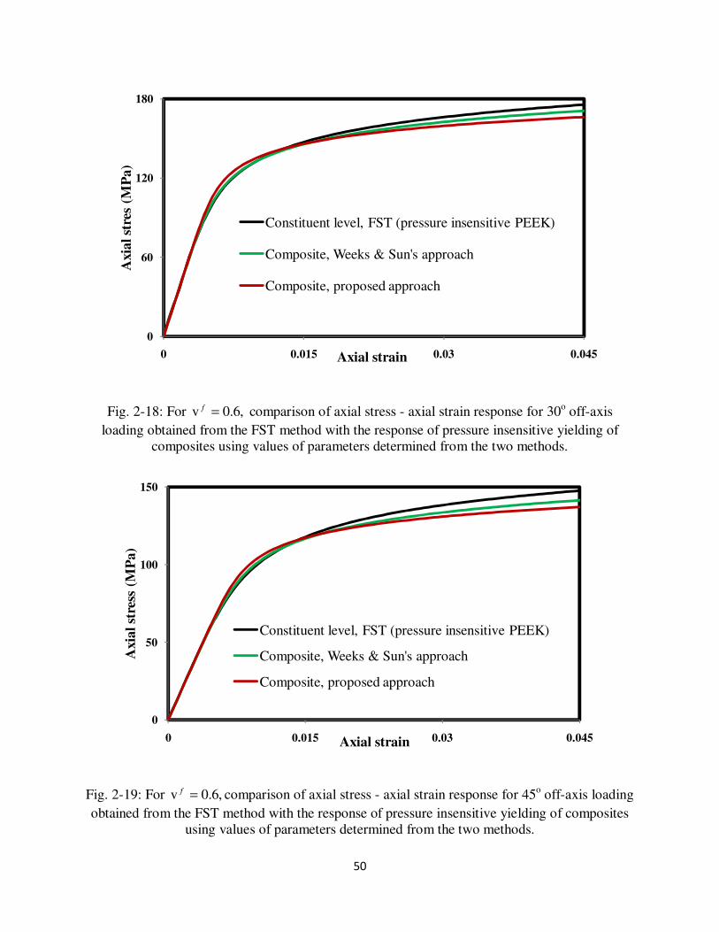
50
Fig. 2-18: For ,6.0v =f comparison of axial stress - axial strain response for 30o off-axis
loading obtained from the FST method with the response of pressure insensitive yielding of
composites using values of parameters determined from the two methods.
Fig. 2-19: For ,6.0v =f comparison of axial stress - axial strain response for 45o off-axis loading
obtained from the FST method with the response of pressure insensitive yielding of composites
using values of parameters determined from the two methods.
0
60
120
180
0 0.015 0.03 0.045
Axia
l st
res
(MP
a)
Axial strain
Constituent level, FST (pressure insensitive PEEK)
Composite, Weeks & Sun's approach
Composite, proposed approach
0
50
100
150
0 0.015 0.03 0.045
Axia
l st
ress
(M
Pa
)
Axial strain
Constituent level, FST (pressure insensitive PEEK)
Composite, Weeks & Sun's approach
Composite, proposed approach

51
For the pressure sensitive yield surface, Figs. 2.20, 2.21 and 2.22 compare the axial stress
versus the axial strain curves for off-axis loading of a lamina obtained using the FST method
with those computed by using the above-listed values of material parameters. Again, the three
sets of curves are close to each other.
Fig. 2-20: For ,6.0v =f comparison of axial stress - axial strain response for 14o off-axis loading
obtained from the FST method with the response of pressure sensitive yielding of composites
using values of parameters determined from the two methods.
0
100
200
300
0 0.015 0.03 0.045
Axia
l s
tres
s (M
Pa)
Axial strain
Constituent level, FST(pressure sensitive PEEK)
Composite, Weeks & Sun's approach
Composite, proposed approach
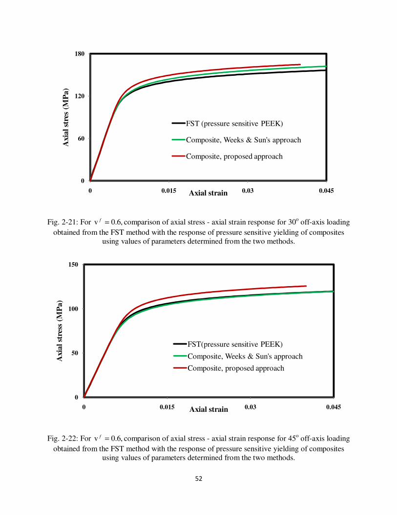
52
Fig. 2-21: For ,6.0v =f comparison of axial stress - axial strain response for 30o off-axis loading
obtained from the FST method with the response of pressure sensitive yielding of composites
using values of parameters determined from the two methods.
Fig. 2-22: For ,6.0v =f comparison of axial stress - axial strain response for 45o off-axis loading
obtained from the FST method with the response of pressure sensitive yielding of composites
using values of parameters determined from the two methods.
0
60
120
180
0 0.015 0.03 0.045
Axia
l st
res
(MP
a)
Axial strain
FST (pressure sensitive PEEK)
Composite, Weeks & Sun's approach
Composite, proposed approach
0
50
100
150
0 0.015 0.03 0.045
Axia
l st
ress
(M
Pa)
Axial strain
FST(pressure sensitive PEEK)
Composite, Weeks & Sun's approach
Composite, proposed approach

53
4.5.4 Dependence of the yield surface upon the fiber volume fraction
We only use the von Mises yield criterion for the matrix and the composite with the
composite modeled as a transversely isotropic material and the fiber axis as the axis of transverse
isotropy; results for the pressure dependent yield surface can be similarly obtained. Furthermore,
we seek an expression for the effective stress of the composite with variables A and N depending
upon the volume fraction of the fibers. We have exhibited in Figs. 2-23 and 2-24 the dependence
of parameters A, N, A12 and A23 upon the volume fraction of fibers ranging from 0.3 to 0.75. The
least squares cubic polynomial fits to the computed values of these variables are listed as insets
in the Figures. It is clear that values of all four parameters rapidly increase with an increase in
the value of the volume fraction of fibers.
Fig. 2-23: Variation with the fiber volume fraction of parameters A and N appearing in the strain
hardening expression for the composite.
A = 2.597(VF)3 - 1.473(VF)2 + 0.116(VF) + 0.396
0
0.2
0.4
0.6
0.8
0.2 0.4 0.6 0.8
A, 10
xN
(G
Pa
)
Fiber volume fraction (VF)
A 10xN
N = 0.107(VF)3 + 0.008(VF)2 - 0.05(VF) + 0.039

54
Fig. 2-24: Variation with the fiber volume fraction of the parameters A12 and A23 appearing in the
yield surface.
5. Conclusions
We have used four micromechanical theories, namely, the Mori-Tanaka, Eshelby’s
equivalent inclusion, the free shear traction method proposed by Robertson and Mall that is a
modification of Aboudi’s method of cells, and Hill’s equivalent energy principle, to find values
of material parameters for elasto-plastic deformations of AS4/PEEK composite. The elasto-
plastic deformations of the matrix are modeled by two yield criteria - the von Mises that
stipulates that plastic deformations are independent of the hydrostatic pressure and the Drucker-
Prager that includes dependence of the yield surface upon the hydrostatic pressure. Whereas the
von Mises yield surface is quadratic in deviatoric stresses the other one has a linear pressure
term.
It is found that for fiber volume fraction, fv , varying from 0.3 to 0.6 the four micro-
mechanics approaches provide noticeably different values of the elastic moduli. For 6.0v =f ,
none of the four theories give values of all five elastic parameters that are close to the
A23 = 158.0(VF)3 - 164.4(VF)2 + 58.44(VF) - 1.5
A12 = 135.8(VF)3 - 138.8(VF)2 + 47.77(VF) - 0.5
4
8
12
16
20
0.2 0.4 0.6 0.8
A12, A
23
Fiber volume fraction (VF)
A23 A12

55
experimental results available in the literature. We note that the difference in the minimum and
the maximum values of Young’s modulus in the direction transverse to fibers found
experimentally by three research groups differ by 20%. Along the fibers, all four theories give
values of Young’s modulus that are very close to each other and can also be found by using the
rule of mixtures. When displacements are applied on the surfaces of a representative volume
element (RVE) to produce a state of simple shear in the lamina plane, the value of the in-plane
shear modulus deduced from Hill’s equivalence energy principle is significantly higher than that
provided by the other three micromechanics approaches as well as the literature experimental
value.
For uniaxial elasto-plastic deformations of the composite lamina with fibers making an
angleθ with the axis of loading, the axial stress versus the axial strain curves computed with the
von Mises yield criterion for the PEEK agree better with the experimental results of Weeks and
Sun than those derived by assuming that the yield criterion is pressure dependent. Assuming that
the plastic deformations of the composite are also independent of the hydrostatic pressure, we
have found values as a function of the volume fraction of fibers of the two material parameters in
the yield surface and the two material parameters that characterize strain hardening of the
composite.
The pressure independent yield surface for the AS4/PEEK composite studied herein is given by
( )
+== p
ij eln NAσ3Fσ where
( ) ( ) ( )[ ]212
21312
22323
23322ij σσ2Aσ2Aσσ
2
1σF +++−=
A = 2.597(VF)3
- 1.473(VF)2
+ 0.116(VF) + 0.396
N = 0.107(VF)3 + 0.008(VF)
2 - 0.050(VF) + 0.039
A23 = 158.0(VF)3 - 164.4(VF)
2 + 58.44(VF) - 1.5
A12 = 135.8(VF)3 - 138.8(VF)
2 + 47.77(VF) - 0.5
and VF equals the volume fraction of the fibers between 0.3 and 0.75. By following a procedure
similar to that used here and simulating homogeneous deformations of the UFPC at different

56
strain rates one can quantify the dependence of the yield stress of the UFPC upon the strain rate
characteristics of the fiber and the matrix.
6. Appendix: comparison of results for elasto-plastic deformations by the M-T and the FST
techniques
We compare results for elasto-plastic deformations derived by using the incremental M-T
and the FST methods. The algorithm for the M-T method has been given by Pettermann et al.
[29], and we study the same composite (carbon fiber reinforced metal matrix) as that analyzed in
[29]. It is assumed that only the matrix deforms plastically deformation, and it is modeled as an
elasto-plastic material obeying the von-Mises yield criterion with the effective stress an affine
function of the effective plastic strain. Values of material parameters for the matrix taken from
[29] are listed in Table 2-2, and those for the carbon are given in Table 2-3 [29].
Table 2-2: Values of material parameters for the matrix.
Elastic modulus Poisson’s ratio Yield stress Hardening modulus
45 GPa 0.35 0.15 GPa 1.28 GPa
Table 2-3: Values of material parameters for the carbon fibers.
E1 E2= E3 G12= G13 1312 νν = 23ν
224 GPa 14 GPa 14 GPa 0.2 0.25
In Fig. 2-25 we have plotted the axial stress versus the axial strain curves for off-axis
loading of a lamina obtained by using the two approaches. In general, the results from the two
method agree well with each other. However, when fibers are inclined at either 60o or 90
o with
the loading axis, yielding occurs at a lower value of the strain for the FST method than that with
the incremental M-T approach. In Figs. 2-26 and 2-27, we have compared results for the cyclic
loading along the fiber direction and the in-plane shear loading. The initial slope (G23) of the

57
shear stress vs. the shear strain curve from the incremental M-T method is larger than that of the
curve computed with the FST approach. The yield stress obtained from results obtained using
the FST method is higher than that deduced from results of the M-T approach, and the FST
method predicts a lower value of the strain hardening modulus than the input value. Thus the
two micromechanics theories that give very close results for axial deformations of a composite
lamina do not provide close values of the yield stress and the hardening modulus for in-plane
shear deformations.
Fig. 2-25: For ,3.0v =f comparison of the axial stress versus the axial strain curves for off-axis
loading computed using the incremental M-T and the FST methods.
0
0.125
0.25
0.375
0.5
0 0.001 0.002 0.003 0.004 0.005
Axia
l st
ress
(G
Pa)
Axial strain
0 degree
20 degree
60 degree
90 degree
M-T [29]
M-T, current analysis
FST

58
Fig. 2-26: For ,4.0v =f comparison of the axial stress versus the axial strain curves for cyclic
loading from the incremental M-T and the FST methods.
Fig. 2-27: For ,4.0v =f comparison of the shear stress versus the shear strain curves computed
using the incremental M-T and the FST approaches.
-0.6
-0.3
0
0.3
0.6
-0.006 -0.003 7E-18 0.003 0.006
Axia
l st
ress
(G
Pa)
Axial strain
MT [29]
FST
MT, current analysis
0
0.025
0.05
0.075
0.1
0 0.005 0.01 0.015 0.02
Sh
ear
stre
ss, ττ ττ 2
3(G
Pa)
2e23
MT [29]
MT, current analysis
FST
59
Acknowledgements
This research was sponsored by the Army Research Laboratory and was accomplished under
Cooperative Agreement Number W911NF-06-2-0014. The views and conclusions contained in
this document are those of the authors and should not be interpreted as representing official
policies, either expressed or implied, of the Army Research Laboratory or the U.S. Government.
The U.S. Government is authorized to reproduce and distribute reprints for Government purposes
notwithstanding any copyright notation hereon. The work was also partially supported by the
Office of Naval Research Grant N00014-1-06-0567 to Virginia Polytechnic Institute and State
University with Dr. Y.D.S. Rajapakse as the program manager.
References
1 Torquato S., Random heterogeneous Media. Springer-Verlag, New York, 2002.
2 Suquet P. M., Continuum micro-mechanics. Springer-Verlag, New York, 1997.
3 Bensoussan A., Lions J.L., Papanicolaou G., Asymptotic analysis for Periodic structures.
North-Holland Publishing Company, New York, 1978.
4 Nemat Nasser S., Hori M., Micromechanics: Overall Properties of Heterogeneous
Materials. North Holland, 2nd edition, Amsterdam, 1999.
5 Mura T., Micromechanics of defects in solids. Kluwer academic press, New York, 1987.
6 Aboudi J., Mechanics of composite materials. Elsevier science publication, Amsterdam,
1991.
7 Tsai S. W., Hahn H. T., Introduction to composite materials. Technomic publication ,
Lancaster PA, 1980.
8 Hyer M. W., Stress analysis of fiber-reinforced composite materials. Destech Pubs Inc.,
Lancaster PA, 2008.
9 Reifsnider K. K., Case S. W., Damage tolerance and durability in material systems. Wiley-
Interscience, New York, 2002.
10 Charalambakis N, Homogenization techniques and micromechanics. A survey and
perspectives. Transactions of ASME, Applied Mechanics Review, 63, 2010, 030803-10.
11 Love B. M., Batra R. C., Determination of effective thermomechanical parameters of a
mixture of two thermoviscoplastic constituents. International journal of plasticity, 22 ,

60
2006, 1026–1061.
12 Bridgman, P. W., Studies in large plastic flow and fracture with special emphasis on the
effects of hydrostatic pressure. McGraw-Hill, New York, 1952.
13 Caddell R. M., Raghava R. S., Atkins A. G., Pressure dependent yield criteria for
polymers. Materials Science and Engineering, 13, 1974, 113-120.
14 Hu L. W., Pae K. D., Inclusion of the hydrostatic stress component in formulation of the
yield condition. Journal of Franklin Institute, 6, 1963, 491–502.
15 Hill R., Elastic behavior of reinforced solids: Some theoretical principles. Journal of the
mechanics and Physics of Solids, 11, 1963, 357-372.
16 Eshelby J. D., The determination of the elastic field of an ellipsoidal inclusion, and related
problems. Proceedings of the Royal Society of London A, 241, 1957, 376-396.
17 Robertson D. D., Mall S., Micromechanical relations for fiber-reinforced composites.
Journal of composite technology and research, 15, 1993, 181-191.
18 Aboudi J., Micromechanical analysis of composites by the method of cells. Transactions of
ASME, Applied Mechanics Reviews, 42, 1989, 193-221.
19 Hill R., The Mathematical Theory of Plasticity. Oxford University Press, New York, 1998.
20 Spencer A. J. M., Plasticity theory for fiber-reinforced composites. Journal of Engineering
Mathematics, 26, 1992, 107-118.
21 Chen J. K., Allahdadi F. A., Sun C. T., A quadratic yield function for fiber-reinforced
composites. Journal of composite materials, 31, 1997, 788-811.
22 Goldberg R. K., Stouffer D. C., Strain rate dependent analysis of a polymer matrix
composite utilizing a micromechanics approach. Journal of composite materials, 36, 2002,
773-793.
23 Bordonaro, C. M, Rate dependent mechanical behavior of high strength plastics:
experiment and modeling. PhD Dissertation, Rensselaer Polytechnic Institute, Troy, New
York, 1995.
24 Kyriakides S., Arseculeratne R., Perry E., Liechti K., On the compressive failure of fiber
reinforced composites. International Journal of Solids and Structures 32, 1995, 689–738.
25 Jen M. H. R., Lee C. H., Strength and life in thermoplastic composite laminates under
static and fatigue loads. Part I: Experimental. International Journal of fatigue, 20, 1998,
605–615.

61
26 Weeks C. A., Sun C. T., Modeling non-linear rate-dependent behavior in fiber-reinforced
composites. Composite Science and Technology, 58, 1998, 603–611.
27 Zheng X., Nonlinear strain rate dependent composite model for explicit finite element
analysis. PhD Dissertation, University of Akron, Akron, Ohio, 2006.
28 Gardner J. P., Micromechanical modeling of composite materials in finite element analysis
using an embedded cell approach. M. Sc. thesis, M.I.T., Cambridge, Massachusetts, 1994.
29 Pettermann H. E., Plankensteiner A. F., Boehm H. J. , Rammerstorfer F. G., A thermo-
elasto-plastic constitutive law for inhomogeneous materials based on an incremental Mori-
Tanaka approach. Computers and Structures, 71, 1999, 197-214.

62
CHAPTER 3: Damage and Failure during Impact Loading of Unidirectional Fiber-
reinforced Laminates
Abstract
We analyze the damage initiation, damage progression, and failure during 3-dimensional
deformations of a unidirectional fiber reinforced laminated composite impacted by a rigid
sphere, and compare computed results with the experimental findings available in the literature.
Damage is assumed to initiate when one of Hashin’s failure criteria is satisfied, and the damage
evolution is modeled by an empirical relation proposed by Matzenmiller, Lubliner and Taylor.
Instead of degrading values of the elastic parameters at a material point we account for the effect
of the damage evolved by appropriately enhancing values of stresses there. The transient
problem is solved by the finite element method (FEM) using 8-node brick elements with 1-point
integration rule, hour-glass control and the explicit conditionally stable central-difference
algorithm for integrating the coupled ordinary differential equations obtained from the Galerkin
formulation of the problem. A user defined subroutine has been developed and implemented in
the commercial FE software ABAQUS. From the strains supplied by ABAQUS it uses the free
shear traction technique of Robertson and Mall (who relaxed the requirement of shear traction
continuity in Aboudi’s method of cells) and values of material parameters of the constituents to
find average stresses in a FE, and checks if Hashin’s failure criteria are satisfied. If damage has
initiated in the material, the subroutine also evaluates the damage developed, computes the
resulting stresses, and provides them back to ABAQUS. The irreversibility of the damage
evolved is considered by requiring that the damage evolved does not decrease during unloading.
The delamination failure mode is simulated by using the cohesive zone model (CZM) and the
Benzeggagh-Kenane criterion for the degradation of material properties in the CZM available in
ABAQUS. The computed time histories of the axial load acting on the impactor are found to
agree well with the experimental one available in the literature, and various damage and failure
modes agree qualitatively with those observed in tests.
Keywords: micro-mechanics, damage, failure, composite laminate, impact

63
1. Introduction
Unidirectional fiber reinforced composites (UFPCs) are being increasingly used in
automotive, aerospace, and defense industries because of their higher specific strength than those
of metallic parts. Furthermore, they can be engineered to obtain optimal material properties in
desired directions. One of the challenging issues in designing a UFPC is delineating various
failure modes, such as fiber breakage, matrix cracking, fiber/matrix debonding, fiber kinking,
and delamination between adjacent plies. The difficulty of the problem is evidenced by the fact
that in the worldwide exercise conducted by Soden et al. [1] very few theories could successfully
predict failure of composite coupons deformed quasistatically. In general, the load carrying
capacity of a structure does not become zero as soon as either failure or damage ensues at one of
its material points and the structure can support additional load before it eventually fails. Thus it
is important to quantify damage caused by the initiation of a failure mode and study the
development and progression of damage and the eventual failure of a structure as the applied
load is increased. For designing UFPCs to resist impact loads it is important to understand
energy dissipated in each failure mode.
Failure and damage in UFPCs can be studied either by using a micro-mechanics approach
that considers constituent level material properties or a continuum damage mechanics approach
in which material properties of the composite have been homogenized and the lamina can be
regarded as a homogeneous and anisotropic body. Generally the micro-mechanics approach
requires considerable computational resources and is impractical for a real size problem. A
middle ground is to use a micromechanics approach to deduce effective properties of a UFPC
and analyze deformations of the structure by regarding it as a continuous body. We adopt this
technique here to analyze the response of a laminated composite plate under impact loading. We
note that the world wide exercise work summarized by Soden et al. [1] lists numerous references
describing failure theories and their predictive capability, and a person interested in UFPCs
should study that work and references listed therein.
Togho and Weng [2] have used a statistical approach based on Weibull’s distribution of
inclusions and the assumption that the inclusion carries no load after it has debonded from the
matrix; they thus generalized Mori-Tanaka’s micromechanics method of deriving effective

64
properties of a UFPC to include the effect of fiber/matrix debonding. In Sun et al.’s [3]
micromechanics-based approach the effect of progressive debonding is considered by gradually
reducing the elastic constants of the inclusions. Nguyen et al. [4] modeled the debonding
process by reducing strengths of the interface between the inclusion and the matrix. Meraghni et
al. [5] and Desrumaux et al. [6] have studied the combined effects of micro-cracks and
debonding on the effective properties of a composite.
Continuum damage theories try to capture effects of microscopic damage by using
essentially Coleman and Gurtin's theory of internal variables [7]. Ladeveze and Dantec [8] have
used this approach to degrade elastic properties of the composite due to fiber breakage and
matrix cracking, and a plasticity theory to account for permanent deformations induced under
shear loading. Hassan and Batra [9] have used three internal variables to characterize damage
due to fiber breakage, matrix cracking and fiber/matrix debonding. The delamination between
adjacent plies was analyzed by using a failure surface that is quadratic in the transverse normal
and the transverse shear stresses. Puck and Schurmann [10] have generalized Hashin’s [11]
stress-based failure criteria, and have proposed techniques to degrade elastic parameters of the
UFPC subsequent to the initiation of a failure mode. Donadon et al. [12] have used a smeared
crack approach to develop a failure model for predicting damage in three-dimensional (3-D)
deformations of a composite structure. Clegg et al. [13] have considered plastic deformations of
a composite by assuming a yield surface quadratic in stresses, and have defined a damage surface
in terms of stresses to consider damage induced softening. The evolution of damage variables is
expressed in terms of a critical strain, fracture energy, fracture stress and a local characteristic
dimension which should help minimize the dependency of computed results upon the finite
element (FE) mesh used to numerically solve a problem. Ma and Cheng [14] have employed the
Ramberg-Osgood plasticity relation to account for nonlinear response of a composite under in-
plane shear loads, and considered three failure modes, namely, fiber breakage, matrix cracking
and interface debonding while studying the initiation and propagation of damage in a composite
plate with a circular hole.
Matzenmiller et al. [15] have proposed that when one of Hashin’s failure criteria is
satisfied at a point in a composite structure, damage ensues at that point and it can be

65
characterized by introducing five internal variables – one for each of the five failure criteria,
namely, fiber breakage in tension and compression, matrix cracking in tension and compression,
and crushing. These internal variables evolve depending upon values of stresses in Hashin’s
failure criteria which are expressed in terms of stress invariants for a transversely isotropic body
and the strength parameters for the composite. Values of the three damage variables depend
upon the values of these five variables, and influence the subsequent values of material elastic
constants. Alternatively, the damage variables can be used to modify the six stress components
that are used to characterize future deformations of the material point. Xiao et al. [16] have used
this approach to study damage during quasistatic punch test for woven fabric composites, and
Williams and Vaziri [17] have evaluated the effectiveness of this technique for studying damage
in carbon fiber reinforced plastics under impact loads.
Here we use Matzenmiller et al.’s [15] damage evolution criteria for studying 3-D
deformations of a 16-ply UFPC laminate impacted at normal incidence by a rigid sphere, and
derive effective elastoplastic properties of the composite by using the free shear traction (FST)
method of Robertson and Mall [18] who relaxed the requirement of the continuity of shear
tractions in Aboudi’s [19] method of cells. The matrix is assumed to deform elasto-plastically
and the fibers elastically. A user defined subroutine has been developed and implemented in the
commercial FE software ABAQUS. This subroutine takes as input from ABAQUS values of the
six strain components at an integration point of a FE, computes effective stresses there by using
the constituent level properties, checks for material failure due to Hashin’s criteria, computes
damage, modifies stresses due to the induced damage, and supplies them to ABAQUS. In the
explicit algorithm adopted here values of effective stresses suffice to find forces due to internal
stresses. Accelerations can be computed from the difference between the applied forces and
forces due to internal stresses. The delamination between adjacent plies is characterized by
using the cohesive zone model (CZM) available in ABAQUS. The computed time histories of
the axial force experienced by the sphere are found to agree well with the experimental results of
Curson et al. [20]. The initiation and the propagation of failure modes agree qualitatively with
those reported by Curson et al.

66
The rest of the paper is organized as follows. Section 2 describes the governing
equations, and a weak formulation of the problem is derived in Section 3 that also briefly
outlines the time integration scheme. Hashin’s failure criteria and the damage evolution
approach of Matzenmiller et al. are described in Sections 4 and 5, respectively. The element
deletion criterion is listed in Section 6, and Section 7 reviews the CZM approach for
characterizing delamination between adjacent plies. The yield surface for modeling plastic
deformations of the matrix is given in Section 8. The micromechanics approach for finding
effective stresses from strains at a point is described in Section 9. We have summarized in
Section 10 the solution algorithm and how the developed subroutine interacts with the FE
software ABAQUS. Computed results for quasistatic deformations of a composite laminate with
different fiber orientations are compared with the corresponding experimental ones of Weeks and
Sun [21] in Section 11. This Section also compares computed results for the impact loading of a
composite laminate with those of Curson et al. [20]. Conclusions of the work are summarized in
Section 12.
2. Problem Formulation
A schematic sketch of the problem studied is exhibited in Fig. 3-1 and resembles that
employed by Curson et al. [20] in their experiments on studying the impact response of
composite laminates. The problem formulation and the solution algorithm are applicable to
study impact of a composite laminate except for the boundary conditions described below that
are specific to the experimental set up of Curson et al. A square n -ply composite laminate of
side, L , and thickness, h , rests on a square steel plate of the size of the laminate except that the
steel plate has a circular hole of diameter, D , at its center. We use global rectangular Cartesian
coordinate axes ( )321 x,x,x (or ( )zy,x, ) to describe deformations of the laminate impacted at
normal incidence by a steel sphere of radius, SR . We note that Curson et al. [20] employed a
hemi-spherical nosed cylindrical impactor in their experiments and observed that it did not
deform much; here we regard the impactor to be rigid. Since the contact area is anticipated to
depend upon the radius of the hemi-spherical nose of the projectile, and the damage induced in
the laminate upon the kinetic energy of the impactor, replacing the cylindrical projectile by a
spherical one should not significantly affect the computed damage in the laminate.

67
Fig. 3-1: Geometric set up for impact test with the impactor shown in green, the composite
laminate in red and the supporting steel plate in blue color.
Recall that fibers exhibit brittle failure at an axial strain of approximately 1% and the
matrix may deform elasto-plastically. Accordingly we assume that elasto-plastic deformations of
the laminate prior to deleting an element are infinitesimal, and the material properties in each
lamina have been homogenized. Furthermore, the lamina material can be modeled as
transversely isotropic with the fiber axis as the axis of transverse isotropy. Thus deformations of
the composite laminate are governed by
ijij,i ρbσuρ +=&& , i=1,2,3 (2.1)
eklijklij εCσ = (2.2)
( )ij,ji,ij u u2
1ε += (2.3)
pij
eijij εdεdεd += (2.4)
Here ρ is the mass density, iu the displacement of a material point along the xi-axis, j
iji,
x
uu
∂
∂= , ijε
the infinitesimal strain tensor, ijσ the stress tensor, ijklC the tensor of material elasticities, ib the
body force per unit mass, a superimposed dot indicates the material time derivative, and eijεd and
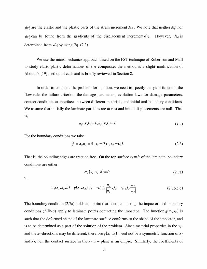
68
pijεd are the elastic and the plastic parts of the strain increment ij εd . We note that neither e
ijεd nor
pijεd can be found from the gradients of the displacement increment idu . However, ij εd is
determined from idu by using Eq. (2.3).
We use the micromechanics approach based on the FST technique of Robertson and Mall
to study elasto-plastic deformations of the composite; the method is a slight modification of
Aboudi’s [19] method of cells and is briefly reviewed in Section 8.
In order to complete the problem formulation, we need to specify the yield function, the
flow rule, the failure criterion, the damage parameters, evolution laws for damage parameters,
contact conditions at interfaces between different materials, and initial and boundary conditions.
We assume that initially the laminate particles are at rest and initial displacements are null. That
is,
0,0)(u0,,0)(u ii == xx & (2.5)
For the boundary conditions we take
0nσf jiji == , L0,x1 = , L0,x2 = (2.6)
That is, the bounding edges are traction free. On the top surface hx3 = of the laminate, boundary
conditions are either
( ) 0h,x,xσ 21i3 = (2.7a)
or
( )2
2322
1
131121213
u
uf-µf,
u
uf-f,x,xgh),x,(xu === µ (2.7b,c,d)
The boundary condition (2.7a) holds at a point that is not contacting the impactor, and boundary
conditions (2.7b-d) apply to laminate points contacting the impactor. The function ( )21 x,xg is
such that the deformed shape of the laminate surface conforms to the shape of the impactor, and
is to be determined as a part of the solution of the problem. Since material properties in the x1-
and the x2-directions may be different, therefore ( )21 x,xg need not be a symmetric function of x1
and x2; i.e., the contact surface in the x1 x2 – plane is an ellipse. Similarly, the coefficients of
69
friction 1µ and 2µ in the x1- and the x2-directions may be different. The normal surface traction,
3f , is also to be determined as a part of the solution of the problem. Because of infinitesimal
deformations considered, we have taken the normal to the deformed surface under the indenter to
be along the x3 -axis as is done in the Hertz contact theory. For a given depth of penetration, the
function ( )21 x,xg can be found by requiring that the deformed shape of the laminate prior to
failure match with that of the impactor. Subsequent to the failure initiation, we require that there
is no interpenetration between the laminate and the impactor. The boundary condition on the
bottom surface 0x3 = of the laminate is
either 0,0,t)x,(xu 213 = or ( ) 0,0,tx,xσ 21i3 = (2.8a,b)
We regard the bottom steel plate to be rigid. The boundary condition (2.8a) holds when
the particle is contacting the steel plate and we impose the boundary condition (2.8b) when the
particle has lifted off from the plate.
At an interface between two adjoining layers, prior to delamination, we assume that
= 0, = 0 (2.9)
where equals the difference in the values of u at the common point of the two layers. These
ensure that the displacements and the surface tractions are continuous across the two layers, or
equivalently, the two layers are perfectly bonded to each other. Subsequent to delamination, the
relation between and of the type given in Section 7 needs to be specified.
At the risk of repetition, we emphasize that except for the initial and the boundary
conditions specified for the problem experimentally studied by Curson et al. [20], the material
presented in Sections 2 through 10 is applicable to any transient problem involving impact and
failure of UFPC laminates.
3. Weak Formulation of Governing Equations and the Time Integration Scheme
Let ( )1,2,3iφi = be a smooth real-valued function defined on the domain, Ω , occupied by
the body in the reference configuration such that 0φi = on the part uΓ of the boundary where

70
displacements are prescribed. Taking the inner product of both sides of Eq. (2.1) with iφ ,
integrating the resulting equation on Ω , and using the divergence theorem, we get
dΩφρbdΩuσdAφfdΩφuρ i
Ω
i
Ω
ji,ij
Γ
ii
Ω
ii
f
∫∫∫∫ +−=&& (3.1)
where surface traction, f , is prescribed on the part uf Γ−Ω∂=Γ of the boundary Ω∂ of the
domain Ω . If we interpret iφ as a virtual displacement then the left-hand side of Eq. (3.1) equals
the work done by inertia forces. The first, the second and the third terms on the right-hand side
of Eq. (3.1) equal, respectively, the work done by surface tractions applied on fΓ , the internal
stresses, and the body force. Thus one can regard Eq. (3.1) as a statement of the principle of
virtual work. Henceforth we take 0b = . We note that the displacement iu in Eq. (3.1) depends
upon the position x of a material particle of Ω and the time t, but the test function iφ depends only
upon x.
In terms of the basis functions ( )N1,2,...,aφa = defined on Ω , we write
( )xx aaii d,t)(u ϕ=
( )xx aaii c)( ϕφ = (3.2a,b)
where summation on the repeated index a is implied. Because of the retention of only N terms
in Eq. (3.2), the right-hand sides of Eqs. (3.2a) and (3.2b) are approximations of functions t),(ui x
and )(i xφ , respectively. Substitution from Eq. (3.2) into Eq. (3.1) and recalling that Eq. (3.1)
holds for all choices of iφ and hence aic , we obtain the following set of coupled ordinary
differential equations for aid .
intai
extaibiab FFdM −=&& , dΩρM
Ω
baab ∫= ϕϕ ,
dAfF
fΓ
aiext
ai ∫= ϕ , dΩσFΩ
ja,ijint
ai ∫= ϕ (3.3a,d)
In Eq. (3.3), M is the mass matrix, and extF and intF are, respectively, due to the applied external
forces and internal stresses. Note that intF depends upon d sinceσ in Eq. (3.3d) is a function of u
and hence ofd .
71
Here we use the finite element (FE) basis functions, and hence the finite element method
(FEM) to solve the problem. That is, we divide the domain Ω into a collection eΩ of non-
overlapping sub-domains called FEs. On each element, eΩ , we select special points, called
nodes. The collection of elements and nodes is called the FE mesh. For the problem studied
here, eΩ is an 8-node rectangular parallelepiped, and aφ is a polynomial defined piecewise onΩ
such that aφ equals 1 at node a and zero at the remaining nodes. Furthermore, aφ vanishes on
those faces of elements that do not pass through node a . Because ( ) abb
a δφ =)(x , ( ) ( )tdtu bib
i =,)(x .
Here )(bx represents the position vector for nodeb . Thus bid equals the displacement of node b
in the xi-direction.
The integrals appearing in Eq. (3.3b-d) can be written as
∑∑∫ ==e
(e)
ab
e Ω
baab MdΩρM
e
ϕϕ , ∑∑ ∫ ==Γ∩Ω e
(e)extai
e
aiext
ai FdAfF
fe
ϕ
∑∑ ∫ ==e
(e)intai
e Ω
ja,ijint
ai FdΩσF
e
ϕ (3.4)
Here (e)
abM is the mass matrix for element e , and the summation is over all elements in the FE
mesh. Generally integrals in Eq. (3.4) are numerically evaluated using a Gauss quadrature rule,
and the accuracy of the results depends upon the number of Gauss integration points used.
Thus the problem of finding an approximate solution of the initial-boundary-value
problem (IBVP) defined by Eqs. (2.1) through (2.9) has been reduced to that of integrating the
system of coupled nonlinear ordinary differential Eqs. (3.3) subject to the following initial
conditions:
( ) ( )0F0dM aibiab = , ( ) ( )0F0dM aibiab =& , (3.5a,b)
where
( ) ( )∫Ω
Ω= du0F iaai 0x,ρϕ , ( ) ( )∫Ω
Ω= du0F iaai 0x,&ρϕ (3.5c,d)
Eqs. (3.5a) and (3.5b) are derived, respectively, from Eq. (3.2) by multiplying both sides with
aρϕ , substituting for ( )tui ,x from Eq. (3.2) and integrating the resulting equations over Ω .

72
The central difference method is used to integrate with respect to time t the coupled
nonlinear ordinary differential Eqs. (3.3) subject to the initial conditions (3.4). The time interval
[ ]T0, of interest is divided into several times steps [ ] [ ],...,,tt,0,t 211 and for the time step [ ]1nn t,t + the
solution )1( +nd at time 1nt + is expressed in terms of the solution )(nd at time nt as follows:
)(
2
)()()1(2
nnnn
tt dddd &&& ∆
+∆+=+ ,
( ))1()()()1(2
++ +∆
+= nnnn
tdddd &&&&&& ,
int
)1()1()1( +++ −= n
ext
nn FFdM &&
(3.6a,b,c)
Here )1( +nd denotes values of nodal displacements at time 1nt + . For a 3-D problem and the domain
Ω having N nodes, d is a 3N-D vector. In Eq. (3.6c) int)1( +nF is unknown since it depends upon
stresses evaluated at time 1nt + which in turn are functions of )1( +nd . In the time step ( )1nn t,t + , Eq.
(3.6) is solved iteratively till the computed solution has converged within the prescribed
tolerance tolδ . That is, in the thk iteration in the time step ( )1nn t,t + , Eq. (3.3a) is written as
)int(
)1(
)(
)1(
)(
)1(
k
n
kext
n
k
n +++ −= FFdM && (3.7)
where )int()1(k
n +F is evaluated from stresses computed with displacements (k)1)(nd + . The iterative process
is stopped when
tolkn
kn
kn
δ≤−
+
−++
)int()1(
)1int()1(
)int()1(
F
FF, aiai
2FF=F (3.8a,b)
The mass matrix M is diagonalized by the row sum technique. That is,
∑=
=N
b
abaa MM1
, no sum on a
0M ab = if ba ≠
(3.9a,b)
For diagonal M Eq. (3.6c) can be easily solved and the explicit algorithm so obtained is
conditionally stable. The time step, n1n t-tt +=∆ , must be less than the time taken for the fastest
wave to travel through the smallest length of any element in the FE mesh. Thus as an element,
eΩ , gets distorted during deformations of the body, its minimum dimension controls the time
step size which can tremendously increase the CPU time. This can be avoided by either
remeshing the deformed region or by deleting severely deformed elements. The former approach
requires mapping values of solution variables from nodes of the old mesh to those of the new
73
mesh, and the latter introduces a void of the size of eΩ in the region. Here we adopt the second
approach and discuss below the damage/failure initiation and the element deletion criteria.
The essential (displacement) boundary conditions prescribed on uΓ are satisfied by
modifying the right-hand of Eq. (3.7) for nodes on uΓ . For example, for node b on uΓ with
( ) ( )ttb buxu =,)( , we replace the resultant force vector ( )int)1()1( ++ − n
extn FF by bu&&bbM (no sum onb ).
4. Damage and Failure Initiation Criteria
Hashin [11] assumed that a UFPC can be modeled as a homogeneous linear elastic
transversely isotropic body with the fiber axis as the axis of transverse isotropy. He proposed
failure criteria in terms of the following five stress invariants:
111 σI = ,33222 σσI += , ( ) 2
23
2
33223 σ4σσI +−=
2
23
2
124σσI += , 2
1233
2
13222313125σσσσσσσ2I −−=
(4.1a-e)
Here a bar superimposed on a stress component implies that its value is with respect to the
material principal axes with the −1x axis aligned along the fiber axis, −2x axis perpendicular to
the −1x axis but in the plane of the lamina and the −3x axis perpendicular to the plane of the
lamina. The failure criteria are assumed to be at most quadratic in stresses; hence they do not
depend upon 5I . We note that
( ) ( ) ( )3322223
2
3322
2
3322223 σσσ4σσσσσ4 −=+−−+ (4.2)
Thus ( )3322
2
23 σσσ − is also a stress invariant. We list below Hashin’s five failure criteria in terms
of the failure indices ( )1,2,3,4,5ifi
= with the understanding that the failure initiates when the
corresponding failure index equals 1.0.
(i) Fiber tensile failure index
( ) 0,SX
f112
2
13
2
12
2
T
112
1>
++
≡ σ
σσσ (4.3)
74
(ii) Fiber compressive failure index
0X
f 11
C
11
2 <≡ σσ
, (4.4)
(iii) Lamina crush index
0Z
f 33
C
33
3 <≡ σσ
, (4.5)
(iv) Matrix tensile failure index
( ) ( ) 0,SSY
f33222
2
13
2
12
2
T
3322
2
23
2
T
33222
4>+
++
−+
+≡ σσ
σσσσσσσ (4.6)
(v) Matrix compressive failure index
( ) ( ) 012
22
<++
+−
+
++
+
−≡
33222
2
13
2
12
2
T
3322
2
23
T
3322
C
3322
T
C2
5,
SS4SYS
Yf σσ
σσσσσσσσσ
(4.7)
In these equations ( )CT
XX is the axial tensile (compressive) stress along the −1x axis.
Furthermore,C
Z is the lamina crush strength, ( )CT
YY andT
S are, respectively, the transverse
tensile (compressive) strengths along the −2x axis and the shear strengths in the −32 xx plane.
The shear strength in either the −31xx plane or the −21xx plane is denoted by S . We note that
1=2
f does not imply fiber failure due to kinking and buckling – these failure modes are not
considered here. 0>33σ generally leads to delamination and is considered separately in Section
7.
5. Damage Evolution
Matzenmiller et al. [15] postulated that when one of the five failure indices in Eqs. (4.3)-
(4.7) equals at least 1, the failure initiates at that point but the material surrounding that point has
not necessarily lost all of its strength. They assumed that the initiation of failure as indicated by

75
Hashin’s failure criteria is synonymous with the initiation of damage at that point. The material
loses its load carrying capacity when the damage accumulated at a material point has reached a
critical value. The damage evolution at a material point is defined in terms of an internal
variable ( )1,2,3,4,5αQα = associated with the failure index αf by the following empirical relation.
( )
−−= αα f1
m
1exp1Q , ( )1,2,3,4,5α = ; 1fα ≥ (5.1)
The value of the parameter m controls the damage evolution rate; a large (small) value of m
implies that the damage evolves quickly (slowly). In the absence of the availability of the
pertinent test data, the value of m is chosen by trial and error.
One way to consider the effect of the damage at a point is to degrade (or reduce) values
of the elastic parameters at that point. Alternatively, one can enhance values of stresses there
because the effective area supporting surface tractions is less than the geometric area because of
the damage induced. The two approaches will have similar consequences when one is using a
stress based failure criteria like Eqs. (4.3) - (4.7). Here we adopt the second approach and
enhance stresses as follows:
Dσσ =ˆ , σDσ =ˆ (5.2a,b)
( ) ( ) ( ) ( ) ( ) ( ) 1
6
1
5
1
4
1
3
1
2
1
1 ω1,ω1,ω1,ω1,ω1,ω1D−−−−−−
−−−−−−= (5.3)
( )321 ,, QQQMaxωω 51 == ,
( )543
,, QQQMaxωω42
== ,
3Qω3 = ,
( )54321
,,,, QQQQQMaxω6
=
(5.4a-f)
Here D is a diagonal matrix, and the right-hand side of Eq. (5.3) gives the diagonal elements of
D . Furthermore, σ is written as a 6-dimensional vector 121323332211 σ,σ,σ,σ,σ,σ . The
motivation for definitions (5.4a-f) of the six damage variables 621 ωωω ,...,, is given in [22].
The irreversibility of the internal variable is accounted for by requiring that 0dQα =
whenever 0dfα ≤ where αdf represents an increment in the value of the failure index α
f when

76
the time is increased from nt to 1nt + . Eq. (5.4a-f) implies that more than one failure index
influences the value of a damage parameter; for example, the value of 3Q affects all six
components of the damage vectorω. Thus even if an internal variable does not increase, the
value of a damage parameter may increase.
The effect of the damage evolved on the subsequent deformations of a material point and
on the value of the failure index αf is considered by replacingσ andσ in Eqs. (4.3)-(4.7) and
(3.6c) by σ and σ , respectively. That isint
)1( +nF in Eq. (3.6c) is evaluated by using1)(nσ +
ˆ rather than
1)(nσ +.
6. Element Deletion Criterion
In the numerical evaluation of integrals appearing in Eq. (3.5) one needs values of stress,
ijσ , at the integration points which depend upon values of the damage variables there. An
element is assumed to have failed when at least one of the five damage variables 521 ,...,, QQQ
exceeds 0.95 and either the ratio of the final volume of the element to its initial volume is less
than 0.1 or more than 4.0 or the axial strain along the fiber direction equals at least 0.05. We
have followed the work of Xiao et al. [16] in adopting this element deletion criterion. Thus for
an element to be deleted not only one of the damage variables must exceed 0.95 but one of the
three auxiliary conditions outlined above must also be satisfied.
7. Cohesive Zone Model for Delamination
The delamination between adjacent layers usually results from the mismatch between the
material properties of the adjacent layers, and strongly depends upon the strength of the interface
between the two layers. Here we use the delamination criterion included in Abaqus.
Accordingly, the description of the criterion follows that given in Abaqus theory manual.
Similar to Hashin’s failure criteria described in Section 4, we assume that the delamination
ensues at a material point on the interface between two contacting layers when the failure index,
delf , defined by
77
( )
<
+
>
+
+
≡
0σ,X
σ
X
σ
0σ,X
σ
X
σ
X
σ
f
33
2
S2
32
2
S1
31
33
2
S2
32
2
S1
31
2
N
33
2
del
ˆˆˆ
ˆˆˆˆ
(7.1a,b)
equals 1. Here S2S1N XXX and , are, respectively, strengths of the interface along the ,−3x the
,−1x and the −2x axes. Subsequent to the initiation of delamination, the relative normal
displacement,
rel
3d , and the relative tangential displacements,
rel
1d and rel
2d , between the adjoining
points of the two layers, are governed by
33
rel
33σdK ˆ= ,
32
rel
22σdK ˆ= ,
31
rel
11σdK ˆ= (7.2)
where 321 KKK and , can be viewed as stiffnesses of the interface along the −1x , the −2x and the
−3x axes, respectively. Thus rel3d measures the relative separation between the surfaces, and rel
1d
and rel
2d the relative sliding between them. Eq. (7.2) relates jumps in tractions and displacements
when Eq. (2.9) does not hold, and implies that subsequent to the onset of delamination the jump
in surface tractions gradually diminish to zero. The values of 321 KKK and , are degraded by the
same damage parameter D defined by
)δδ(δ
)δδ(δD
0
m
f
m
max
m
0
m
max
m
f
m~~~
~~~
−
−=
(7.3)
where
( ) ( ) ( )2222
mδ~ rel
3
rel
2
rel
1 ddd ++=
mtt
max
m δδn
~max
~
0 ≤≤=
η
TOTAL
IIIIIICIICIC
o
m
o
effG
GG)G2(G2Gδt
+−+=
~
( ) ( ) ( )
( ) ( )
<+
>++=
0σ ,σσ
0σ ,σσσt
33
2
32
2
31
33
2
33
2
32
2
312
eff
ˆˆˆ
ˆˆˆˆ
(7.4a-d)

78
The damage evolution law given by Eq. (7.4) is due to Benzeggah and Kenane [23].
Furthermore, o
eff
o
mtδ and
~ are equal, respectively, to the values of
effmtδ and
~at the instant of the
initiation of the delamination, and η is a material parameter. The new value of 1K , for example,
is given by
( )D1KK 1
dam
1 −= (7.5)
8. Elastoplastic Deformations of the Matrix
We assume that fibers deform elastically and the matrix elasto-plastically. As reported
by Raghava and Caddell [24], unlike most metals, plastic deformations of polymers generally
depend upon the hydrostatic pressure. Here we presume that plastic deformations of the polymer
(PEEK) obey the von Mises yield criterion. The von Mises potential function [28] is given by
( ) ( ) ( ) ( ) 212
213
223
22211
21133
23322ij 2σ2σ2σσσ
3
1σσ
3
1σσ
3
1σ2F +++−+−+−= (8.1)
Thus we have neglected the dependence of the yield surface upon the hydrostatic pressure.
We use the associative flow rule of plasticity to find p
ijdε . Thus
ij
p
ijσ
Fdλd
∂
∂=ε (8.2)
where dλ is the proportionality (also sometimes called the consistency) parameter. The effective
stress associated with the yield function given in Eq. (8.1) is defined as
( )ijσ3Fσ = (8.3)
and the effective plastic strain, pε , by requiring that in any incremental deformation,
p
ij
p
ij εdσσd =ε (8.4)
Substituting forp
ijdε from Eq. (8.2) into Eq. (8.4) and using Eq. (8.3) we get
σ
σd
2H
3
σ
εd
2
3dλ
m
P
== (8.5)
where the strain-hardening modulus, P
m
d
dH
ε
σ= , has been assumed to be positive. The function
( )pmH ε is found from experimental data.
79
Taking the differential of both sides of Eq. (8.3) we get
ijijkk
ij dσδ3
σσ
σ2
3σd
−= (8.6)
Substituting for dλ from Eq. (8.5) and σd from Eq. (8.6) into Eq. (8.2) we get
pq
P
ijpqpqpqll
pqijkk
ij2m
p
ij dσSdσδ3
σσ
σσ
σ4H
9d =
−
−
= δε
3 (8.7)
PS may be called the plastic compliance matrix of the polymer.
Expressing incremental strains in terms of incremental stresses we have
σSσSεPE ddd += (8.8)
where 1E CS −= is the elastic compliance matrix for the polymer. Hence
( ) εSSσPE dd
1−+= (8.9)
which relates incremental stresses to incremental strains and the current stresses.
9. Micromechanics Approach for Finding Stresses in a Finite Element
The iterative solution of the initial-boundary-value problem formulated in Section 3 for
the time interval ( )1nn t,t + provides values of incremental displacements and hence incremental
strainsij∆ε in a FE. We use the free shear traction (FST) scheme of Robertson and Mall [18] to
find the stress increment corresponding to the strain incrementij∆ε and known values of material
parameters for the matrix and the fiber as well as of the fiber volume fraction. Details of this
technique are described in Chapter 2, and are omitted here. The stress increment so computed is
used to update the force vector)int(
)1(
k
n+F in Eq. (3.7).
Robertson and Mall [18] modified Aboudi’s [19] method of cells by relaxing the
continuity of tractions across the interfaces between four cells of which one is made of the fiber
and the other three of the matrix. The ratio of the volume of the fiber cell to that of the four cells
combined equals the volume fraction, fv , of fibers in the composite. Since we find stresses in
the fiber and the matrix before finding the average stress in the FE which is divided into the four
cells, we could potentially use failure and damage criteria at the constituent level. This approach
could simulate well the failure of fibers and of the matrix but will not be very good for predicting

80
debonding of fibers from the matrix. Gardner [25] has incorporated fiber/matrix debonding in
Aboudi’s [18] method of cells by inserting springs between faces of adjoining cells. The
approach is similar to the cohesive zone modeling (CZM) technique discussed above for
simulating delamination between adjoining layers.
10. Summary of the Solution Algorithm
The numerical solution of a given initial-boundary-value problem involves the following
steps.
(i) Solve Eq. (3.7) for1)(k
1)(nd++ and from incremental displacements
(k)
1)(n
1)(k
1)(n ddd +++ −=∆ , find
incremental strains by using Eqs. (3.2a) and (2.3). Check for convergence of the solution
by using Eq. (3.8). When the solution has converged, go to step (v).
(ii) Use the micromechanics approach of Section 9 to findijσ∆ and hence
1)(n+σ .
(iii) Find stress1)(n+σ in material principal coordinates by using tensor transformation rules and
check if any one of the five failure indices, αf , either equals or exceeds 1.
(iv) If 1≥αf , use Eqs. (5.1) - (5.4) to find1)(n+σ . Return to step (i).
(v) Check for delamination between adjoining layers by finding the value of delf defined by
Eq. (7.1).
(vi) If the solution time 1nt + is less than the final time T for the computation of the solution,
increment 1nt + by t∆ and go to step (i). Otherwise, post-process stresses, strains and
displacements to find quantities of interest.
11.1 Numerical Results and Discussion
The composite laminates studied in this work are AS4/PEEK with material properties of
the fiber and the matrix listed in Tables 3-1 and 3-2, respectively. Values of strength parameters
appearing in Hashin’s failure initiation criteria (4.3) – (4.7) are given in Table 3-3.

81
Table 3-1: Values of material parameters for the AS4 fiber [26].
1E 32 EE = 1312 GG = 23G 1312 νν = 23ν
234 GPa 14 GPa 27.6 GPa 5.6 GPa 0.2 0.25
Table 3-2: Values of material parameters for PEEK polymer [27].
E ν
4 GPa 0.35
Table 3-3: Values in GPa of strength parameters for the AS4/PEEK composite
with 60% volume fraction of fibers [28].
TX CX TY CY CZ
TS S
1.4 1.1 0.08 0.21 3.0 0.07 0.07
Values of strength parameters ( )TT YX , ( )CC YX were obtained as the last data points
reported in the experimental uniaxial tension and uniaxial compression tests with the loading
along (perpendicular to) to the fiber axis [28]. It is clear that the composite strength for uniaxial
tensile load along the fiber axis is nearly 21% more than that for the compressive load.
However, for uniaxial transverse load, the strength in compression is about 2.6 times that in
tension. The tensile strength in the transverse direction is nearly 1/17th
of that in the axial
direction. The value of the crush strength, CZ , has not been reported by several researchers and
values as high as 10 GPa have been used [29]. Here we have estimated GPa 3=CZ . A flat
laminate impacted by a sphere normal to the face sheet usually does not fail due to crushing; thus
the precise value of CZ is not critical for our work. The value of the shear strength parameter,
,S is taken equal to the last data point reported in the shear stress-shear strain curve of
Kyriakides et al. [28], and we have set SST = .

82
Goldberg and Stouffer’s [27] reported experimental uniaxial stress-strain curve for PEEK
tested at the strain rate of 10-6
/s by Bordonaro [30]; it is reproduced in Fig. 3-2. For a given
value of the axial stress, 11σ , the value of the axial plastic strain, p
11ε , is computed by using the
relation
E
σε 11
11
p
11 −=ε (11.1)
where 4GPa=E as listed in Table 3-2 and provided by Goldberg and Stouffer [27]. Points
( )11
p
11 σ,ε are plotted in Fig. 3-3. A least squares fit to these data points with a regression
coefficient of 0.98 is
−=
N
Aσxpepε
for
MPa40σ MPa94 ≥≥ (11.2)
where A = 153 MPa and N = 13.86 MPa. In Eq. (11.2) we have set p
11
p εε = and 11σσ = which
follow from Eqs. (8.4) and (8.5).
Fig. 3-2: Computed and experimental axial stress vs. axial strain curves for PEEK polymer.
0
25
50
75
100
0 0.01 0.02 0.03 0.04 0.05
Axia
l st
ress
(M
Pa
)
Axial strain
Current numerical analysis
Expt. [30]

83
Fig. 3-3: Effective stress versus effective plastic strain curve for PEEK obtained from the
experimental axial stress versus axial strain curve.
11.2 Comparison of Computed Results with Experimental Findings
11.2.1 Simple quasistatic deformations
In these simulations m in Eq. (5.1) is assigned the value 100. Thus the damage evolves
very rapidly at a material point. There is no experimental data to determine the rate of evolution
for the damage. The value of 100=m is probably appropriate for the fiber breakage but may be
too high for the matrix failure mode.
We have compared in Fig. 3-4a-e computed results with the experimental ones for
uniaxial tensile and compressive loading along and perpendicular to the fiber axis as well as
simple shear deformations in the x1x2-plane. The specimen is assumed to deform
homogeneously, thus one FE is used to simulate these tests. Also the stress-strain relations, the
damage criteria and the damage evolution laws have been assumed to be independent of the
strain rate. Hence the loading rate does not affect the computed stresses for strains prescribed
40
60
80
100
0 0.006 0.012 0.018 0.024
Eff
ecti
ve
stre
ss (
MP
a)
Effective plastic strain
Least squares fit
From expt.[30]

84
via assigning appropriate displacements at the bounding surfaces. The developed subroutine,
VUMAT, in conjunction with the commercial FE software ABAQUS is used to compute results
using an 8-node brick element with one-point integration rule. The possible emergence of
spurious energy modes with one-point integration rule is suppressed by using the default values
of parameters in the hourglass shape functions.
Fig. 3-4a: Comparison of the experimental and the numerical axial stress versus the axial strain
curves for AS4/PEEK composite for tension test along the fiber direction.
0
0.4
0.8
1.2
1.6
0 0.004 0.008 0.012
Axia
l s
tres
s (G
Pa
)
Axial strain
FST, elastic-plastic with damage
Expt. [28]

85
Fig. 3-4b: Comparison of the experimental and the numerical axial stress versus the axial strain
curves for AS4/PEEK composite for compression test along the fiber direction.
It is clear from results depicted in Fig. 3-4a,b that the present approach mimics well the
experimentally observed axial stress versus the axial strain response in tension but not so well in
compression. The magnitude of the experimental axial strain at failure in tension and
compression equals about 1.03%. The computed value of the axial strain at failure in tension is
close to 1.03% but that in compression is about 0.8% which can be attributed to the fact that the
value of CX is less than that of TX . We note that there is no distinction between the uniaxial
compressive and tensile loading in the method of cells and our formulation of the elasto-plastic
deformations of the matrix. Young’s modulus from the experimental curve for uniaxial
compressive loading is less than that for uniaxial tensile loading. The vertical drop at failure in
the experimental curves is our concoction since that portion of the curve was not captured in
experiments.
0
0.4
0.8
1.2
0 0.004 0.008
Axia
l s
tres
s (
GP
a)
Axial strain
FST, elastic-plastic with damage
Expt. [28]

86
For uniaxial tensile and compressive loading in the transverse (x2-) direction, see Fig. 3-
4c,d, the computed values of the transverse axial strain at failure in compression is nearly four
times that in tension primarily because 6.2=TC YY and the composite deforms elasto-plastically
in compression but mostly elastically in tension. The curves from the computed results are close
to those from experimental findings but the corresponding values of the strain at failure differ by
about 16%. Both for the tensile and the compressive loading, the experimental value of Young’s
modulus is higher than that computed from the micromechanics approach.
Fig. 3-4c: Comparison of the experimental and the numerical axial stress versus the axial strain
curves for AS4/PEEK composite for tension test normal to the fiber direction.
0
0.03
0.06
0.09
0 0.004 0.008 0.012
Axia
l s
tres
s (
GP
a)
Axial strain
FST, elastic-plastic with damage
Expt. [28]

87
Fig. 3-4d: Comparison of experimental and numerical results for AS4-PEEK composites for
compression test normal to the fiber direction.
For simple shear deformations in the x1x2-plane, there are significant plastic deformations
induced in the composite. The shear stress versus shear strain curve from the computed results
agrees well with that from the test data till a shear strain of 4% when the specimen failed in the
tests. The computed shear strain at failure of 5.2% exceeds the experimental one by 30%.
0
0.075
0.15
0.225
0 0.01 0.02 0.03 0.04
Axia
l s
tres
s (
GP
a)
Axial strain
FST, elastic-plastic with damage
FST, elastic-plastic with no damage
Expt. [28]
FST, elastic with damage
FST, elastic with no damage

88
Fig. 3-4e: Comparison of the experimental and the numerical axial stress versus the axial strain
curves for AS4/PEEK composite for shear deformations in the plane of the lamina.
We now simulate experiments conducted by Weeks and Sun [21] involving uniaxial
loads on a lamina with unidirectional fibers inclined at an angleθ to the loading axis. These are
simulated by first finding strains in the material principal axes, supplying these to the user
defined subroutine, VUMAT, computing stresses by the FST method in the material principal
coordinates, checking for Hashin’s failure criteria, modifying them due to the damage induced,
transforming the modified stresses to the global coordinate axes, and supplying these to
ABAQUS for the next iteration or the load step (time increment). Results presented in Figs. 3-
5a,b,c for θ = 14o, 30
o and 45
o clearly show that, prior to the onset of failure, the computed axial
stress versus axial strain curves agree well with the corresponding experimental ones. The
maximum difference between the computed and the experimental values of the axial strain at
failure is less than 20%.
0
0.02
0.04
0.06
0.08
0 0.02 0.04 0.06
Sh
ear
str
ess
σσ σσ12 (
GP
a)
Shear strain (2*εεεε12)
FST, elastic-plastic with damage
FST, elastic-plastic with no damage
Expt. [28]
FST, Elastic with damage
FST, Elastic with no damage

89
Fig. 3-5a: Comparison of the experimental and the computed axial stress versus axial strain
curves for AS4/PEEK composite with fibers making an angle of 14o with the loading axis.
Fig. 3-5b: Comparison of the experimental and the computed axial stress versus axial strain
curves for AS4/PEEK composite with fibers making an angle of 30o with the loading axis.
0
0.1
0.2
0.3
0 0.004 0.008 0.012
Axia
l s
tres
s (G
Pa
)
Axial strain
FST, elastic-plastic with damage
FST, elastic-plastic with no damage
Expt. [21]
FST, elastic with damage
FST, elastic with no damage
0
0.04
0.08
0.12
0.16
0 0.006 0.012 0.018
Axia
l s
tres
s (G
Pa)
Axial strain
FST, elastic-plastic with damage
FST, elastic-plastic with no damage
Expt. [21]
FST, elastic with damage
FST, elastic with no damage

90
Fig. 3-5c: Comparison of the experimental and the computed axial stress versus axial strain
curves for AS4/PEEK composite with fibers making an angle of 45o with the loading axis.
11.2.2 Impact Loading of a Composite Laminate
We now simulate transient deformations of a 75 mm x 75 mm x 2 mm 16-layer
2S90] 45/ 0/ [-45/ AS4/PEEK composite plate impacted at normal incidence by a 500 g 12.7 mm
diameter rigid sphere. Fig. 3-6 shows the stacking sequence of the top half of the symmetric
composite plate, the bottom half is its mirror image.
0
0.04
0.08
0.12
0 0.005 0.01 0.015
Axia
l s
tres
s (G
Pa)
Axial strain
FST, elastic-plastic with damage
FST, elastic-plastic with no damage
Expt. [21]
FST, elastic with damage
FST, elastic with no damage

91
Fig. 3-6: Stacking sequence of the top half of the symmetric 16 layer composite laminate.
As displayed in Fig. 3-1 the composite laminate is supported on a rigid steel plate having
a 50 mm diameter circular opening. The assumption of modeling the sphere as rigid is
reasonable since the 500 g 12.7 mm hemispherical nosed cylindrical impactor used in
experiments underwent very little deformations. All three displacement components of the base
plate are set equal to zero, and the coefficients of friction 1µ and 2µ (cf. Eq. (2.7)) between the
spherical impactor and the composite laminate are set equal to 0.25. Values of material
parameters in Eqs. (7.1) and (7.4) are listed below in Table 3-4; values of GIC, GIIC, GIIIC and η
used herein are typical for carbon fiber reinforced polymer composites, see e.g. [31]. There is,
in general, considerable scatter in values of strength parameters TX and TY ; for example, Curson

92
et al. [20] reported GPa 2.1=TX and GPa 0.135=TY which are higher than those listed in Table
3-3.
Table 3-4: Values of interfacial strength parameters for the composite laminate [31].
NX
S1 S2X X=
ICG
IIC IIICG G= η
80 MPa 150 MPa 150 J/m2 500 J/m
2 1.7
Because of infinitesimal deformations of the laminate the contact force, FC, acting on the
rigid sphere can be defined as
21
A
33c dxdxσF
c
∫= ˆ (11.3)
where C
A is the time-dependent contact surface.
The time step size is adaptively controlled in ABAQUS by finding the maximum
frequency of the structure. We further scaled it down to 25% of that computed by ABAQUS
using the stability limit.
We used the default values 0.06 and 1.2, respectively, for the linear and the quadratic
artificial bulk viscosities. The linear bulk viscosity damps out “ringing” in the highest element
frequency and the quadratic bulk viscosity is introduced only in those elements that have
compressive volume strain to prevent them from collapsing. These viscosities are introduced by
adding an artificial hydrodynamic pressure to the right-hand side of Eq. (2.2).
Numerical simulations involving contact problems using ABAQUS EXPLICIT were
carried out using the penalty based algorithm “GENERAL CONTACT" in which one does not
have to define the "MASTER" and the "SLAVE" surfaces. The algorithm introduces an
additional stiffness when it detects the penetrating body. The value of the penalty stiffness
influences the time step size, and high values of the penalty stiffness not only drastically reduce
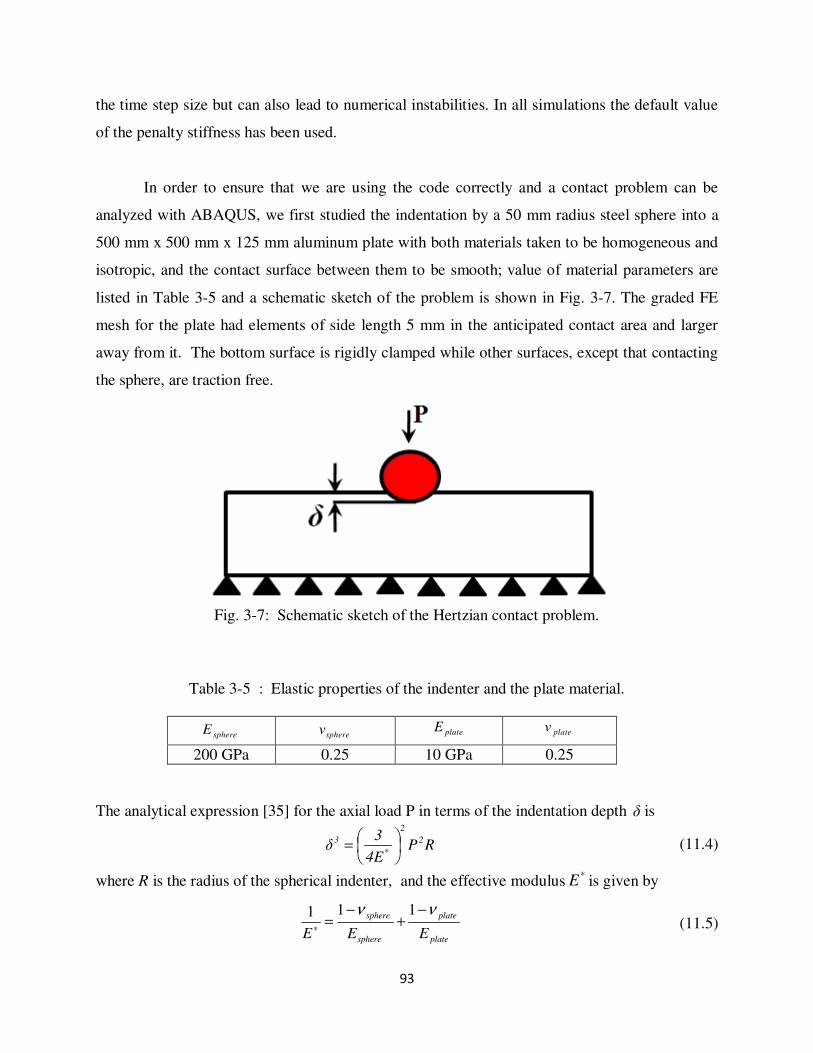
93
the time step size but can also lead to numerical instabilities. In all simulations the default value
of the penalty stiffness has been used.
In order to ensure that we are using the code correctly and a contact problem can be
analyzed with ABAQUS, we first studied the indentation by a 50 mm radius steel sphere into a
500 mm x 500 mm x 125 mm aluminum plate with both materials taken to be homogeneous and
isotropic, and the contact surface between them to be smooth; value of material parameters are
listed in Table 3-5 and a schematic sketch of the problem is shown in Fig. 3-7. The graded FE
mesh for the plate had elements of side length 5 mm in the anticipated contact area and larger
away from it. The bottom surface is rigidly clamped while other surfaces, except that contacting
the sphere, are traction free.
Fig. 3-7: Schematic sketch of the Hertzian contact problem.
Table 3-5 : Elastic properties of the indenter and the plate material.
sphereE sphereν plateE plateν
200 GPa 0.25 10 GPa 0.25
The analytical expression [35] for the axial load P in terms of the indentation depth δ is
RP4E
3δ 2
2
*
3
=
(11.4)
where R is the radius of the spherical indenter, and the effective modulus*E is given by
plate
plate
sphere
sphere
* EEE
νν −+
−=
111
(11.5)

94
The computed contact force acting on the sphere versus the indentation depth is
compared with that obtained from the analytical solution in Fig. 3-7. The two curves agree well
with each other for the indentation depth up to 1.5 mm after which they begin to deviate. There
are oscillations in the numerical solution because we solved a transient problem whereas the
analytical solution is for a static problem. This exercise insures that we are correctly using the
software, and one can get good results for a contact problem with the software.
Fig. 3-8: Comparison of the computed contact force versus the indentation depth with that
obtained from the analytical solution.
For the initial velocity = 4 m/s of the sphere (initial kinetic energy = 4 J), we have
compared in Fig. 3-9 the computed time history of the contact force, CF , with the experimental
one. The time is reckoned from the instant of contact between the sphere and the laminate, and
results have been computed for two sets of values of TX and TY listed in subsection 11.2.2.
During the initial 0.25 ms of contact, the total force between the sphere and the laminate is more
than that measured experimentally, and different values of TX and TY have negligible effect on
the magnitude of CF . For ms, 0.25>t the lower values of TX and TY result in a smaller value of
0
120
240
360
0 0.75 1.5 2.25
Con
tact
forc
e (K
N)
Depth of penetration (mm)
Numerical simulation
Analytical solution

95
CF . The time,pt , when the two computed values of CF peak agrees well with that when the
experimentally measured CF has the maximum value. In the neighborhood of ptt = the
amplitude of oscillations in the experimental values of CF is considerably more than that in the
computed values of CF . The time, ft , when the sphere looses contact with the laminate is the
least for GPa 2.1=TX and GPa 135.0=TY , and the most for GPa 4.1=TX and GPa 08.0=TY .
The sphere remains in contact with the laminate for about 2.5 ms.
Fig. 3-9: Comparison of the computed and the experimental time histories of the contact force.
We have displayed in Fig. 3-10a-f fringe plots of stresses at ms 0.55=t , this is the time
when a failure first occurs in the composite. In order to clearly show stresses within the
laminate, the system has been cut by the plane x2 = constant that passes through the sphere
0
1
2
3
0 1 2 3
Co
nta
ct f
orc
e (K
N)
Time (ms)
Current analysis, high strength
Expt.[20]
Current analysis, low strength

96
center. Peak values of 11σ close to 1.5 GPa occur in the four elements directly underneath the
spherical impactor that are on the bottom surface of the laminate. In the third and the fourth ply
from the bottom surface, one can see large values, around 1.28 GPa, of 11σ . The average values
of Young's moduli E1 and E2 are equal. However, the 3-D analysis seems to capture effects of
the location of plies. The magnitudes of stresses are essentially either symmetric or anti-
symmetric about the plane x2 = constant passing through the sphere center. The maximum value
of 12σ is about 45% of the maximum value of 11σ . The magnitudes of 13σ and 23σ are
approximately equal and are about 4.5% of the maximum value of 11σ . 33σ varies from 82.5
MPa in tension along the periphery of the impactor to -0.28 GPa in compression below the
impactor. Since TS1N 0.11X0.5XX ≅≅ , the plies in the bottom half of the laminate have
delaminated in the region directly underneath the sphere.
Fig. 3-10a: Fringe plot of stress 11σ at t = 0.55 ms after impact.
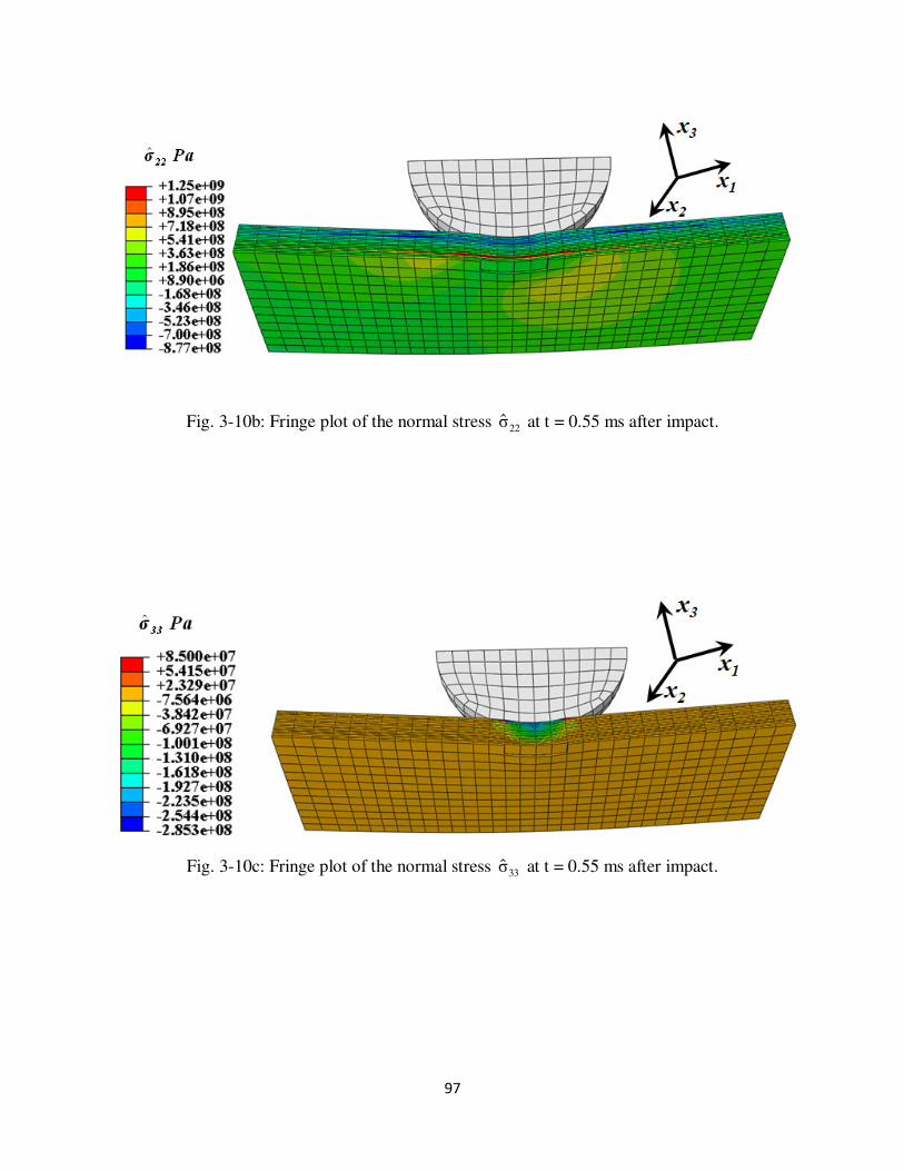
97
Fig. 3-10b: Fringe plot of the normal stress 22σ at t = 0.55 ms after impact.
Fig. 3-10c: Fringe plot of the normal stress 33σ at t = 0.55 ms after impact.
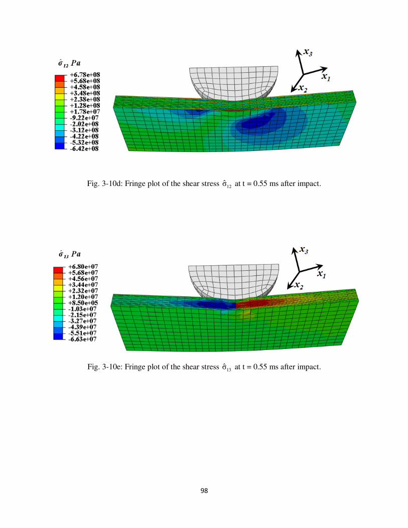
98
Fig. 3-10d: Fringe plot of the shear stress 12σ at t = 0.55 ms after impact.
Fig. 3-10e: Fringe plot of the shear stress 13σ at t = 0.55 ms after impact.

99
Fig. 3-10f: Fringe plot of the shear stress 23σ at t = 0.55 ms after impact.
At ms 1.1=t we have exhibited in Fig. 3-11a-f fringe plots of the internal variables
Dφφφφφ54321
and ,,,, that characterize damage due to fiber tensile failure, fiber compressive
failure, laminate crushing, the matrix tensile failure, the matrix compressive failure, and the
delamination between adjacent plies, respectively. In the magnified view of Fig. 3-11b one can
see several elements that failed due to the matrix failing in tension and were deleted during the
analysis. There are several elements directly underneath the spherical impactor in Fig. 3-11c in
which the fibers failed due to the excessive axial compressive stress. Fringe plots of the internal
variable, 3φ , associated with the crush damage shown in Fig. 3-11e reveal that there is no
damage induced due to the laminate crushing. However, fringe plots of the damage variable, D ,
displayed in Fig. 3-11f lead to the conclusion that the delamination between adjacent plies occurs
over a very large region.

100
Fig. 3-11a, b: Fringe plots of internal variables Q1 and Q4 associated with the fiber and the
matrix tensile damage at t = 1.1 ms; and a magnified view of the severely damaged region.
Fig. 3-11c,d: Fringe plots of internal variables Q2 and Q5 associated with the fiber and the matrix
compressive damage at t = 1.1 ms.
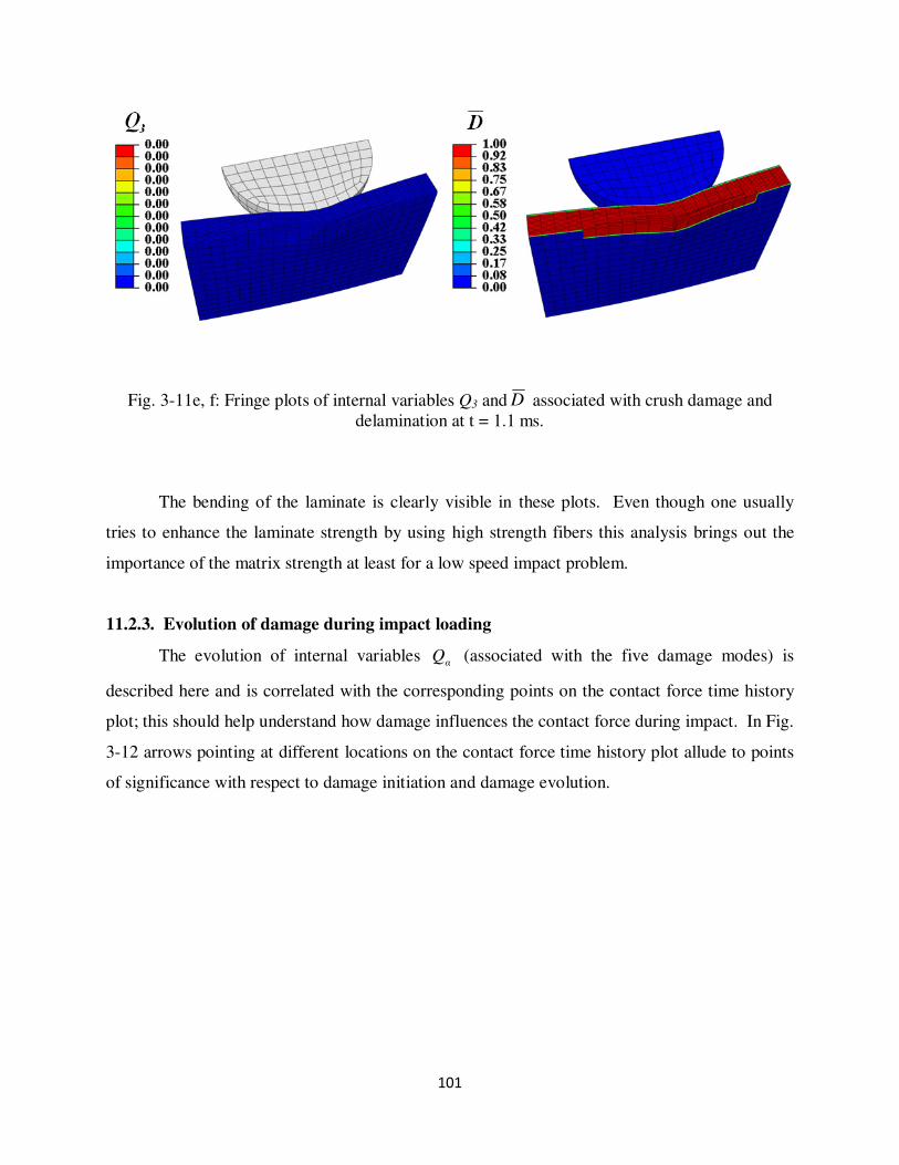
101
Fig. 3-11e, f: Fringe plots of internal variables Q3 and D associated with crush damage and
delamination at t = 1.1 ms.
The bending of the laminate is clearly visible in these plots. Even though one usually
tries to enhance the laminate strength by using high strength fibers this analysis brings out the
importance of the matrix strength at least for a low speed impact problem.
11.2.3. Evolution of damage during impact loading
The evolution of internal variables αQ (associated with the five damage modes) is
described here and is correlated with the corresponding points on the contact force time history
plot; this should help understand how damage influences the contact force during impact. In Fig.
3-12 arrows pointing at different locations on the contact force time history plot allude to points
of significance with respect to damage initiation and damage evolution.

102
Fig. 3-12: Contact force time history plot with points of significance for the damage initiation
and propagation.
Our analysis predicts that the fiber compressive damage associated with the internal
variable Q2 initiates first at ~ 0.25 ms, and occurs at a point contacting the impactor; this is
indicated as '1' in Fig. 3-12. The corresponding fringe plot of Q2 shown in Fig 3-13a suggest that
the damage due to fiber compression is localized in a narrow region below the impactor and it
does not affect the contact force.

103
Fig. 3-13a: Fringe plot of internal variable Q2 (fiber compressive damage) at ms. 0.25t ≈
The matrix tensile damage, quantified by values of Q4, initiates next at the bottom-most
layer of the composite plate at ~ 0.3 ms after impact. It is indicated as point '2' in Fig. 3-12 and
fringe plots of the fiber compressive and the matrix tensile damage are shown in Fig. 3-13b. The
value of the fiber compressive damage variable has increased to nearly1 but the damage remains
localized at points below the impactor. The initiation of the two damage modes does not seem to
influence the force between the impactor and the laminate. Even though the value of the internal
variable has exceeded 0.95, the other two auxiliary criteria given in Section 6 for element
deletion have not been satisfied.

104
Fig. 3-13b: Fringe plots of internal variables Q2 (fiber compressive damage) and Q4 (matrix
tensile damage) at ms. 0.3t ≈
The fiber tensile damage, signified by values of Q1, initiates along the top-most layers of
the composite plate at ~0.4 ms after impact and is indicated as point '3' in Fig. 3-12. The
corresponding fringe plots for the three damage modes shown in Fig 3-13c suggest that the
matrix tensile damage has increased in the bottom layers of the plate while the fiber compressive
damage has spread out in the top layers of the plate. Also noticeable in the contact force time
history plot is a sharp drop in the contact force at this instant. This drop is attributed to both the
fiber tensile damage and the growth of the fiber compressive and the matrix tensile damage
modes. The drop in the contact force is followed by a further increase in the contact force but

105
now at a rate less than that prior to the drop. Schoeppner and Abrate [32] called this point as the
"damage threshold load" (DTL). DTL is the impact load at which there is sufficient accumulation
of damage in the composite plate causing a reduction in its stiffness and hence a change in the
slope in the contact force time history plot.
Fig. 3-13c: Fringe plots of internal variables Q1 (matrix tensile damage), Q2 (fiber compressive
damage) and Q4 (matrix tensile damage) at ms. 0.4t ≈
The compressive matrix damage, decipherable from values of Q5, initiates at ms 0.45t ≈
but is limited to points near the top surface of the composite plate. At mst 0.52 ≈ the second drop
in the contact force is observed (indicated as '4' in Fig. 3-12). The fringe plot of the compressive
damage mode shown in Fig. 3-13d indicates that the damage is insignificant to warrant a drop in
the contact force. The fringe plot of the fiber tensile damage mode reveals that significant fiber
tensile damage occurs in the bottom layers of the composite plate but the region of the fiber
tensile damage has not grown in the top layers of the plate. The magnitudes of other damage
modes have also not increased much. Hence it can be concluded that the second drop in the

106
contact force at point '4' is due to the accumulation of the fiber tensile damage along the bottom
layers of the composite laminate.
Fig. 3-13d: Fringe plots of internal variables Q1 (matrix tensile damage), Q2 (fiber compressive
damage), Q4 (matrix tensile damage) and Q5 (matrix compressive damage) at ms.t 0.52 ≈
At ms 0.55t ≈ , indicated as point '5' in Fig. 3-12, we see another sharp drop in the
contact force whose magnitude is much larger than that of the previous two drops in the contact
force. Fringe plots of the internal variables Q1 (fiber tensile damage mode) and Q4 (matrix tensile
damage mode) shown in Fig 3-13e indicate that elements have been deleted from the FE mesh
which may have reduced the laminate stiffness and caused the contact force to drop. The other
damage modes are primarily restricted to the top layers of the composite plate, and no element
has been deleted in that region.
At ms 1.25t ≈ the impactor begins to rebound (indicated as point '6' in Fig. 3-12). A
significant number of elements have failed by this time.

107
Fig. 3-13e: Fringe plots of internal variables Q1 (fiber tensile damage) and Q4 (matrix tensile
damage) at ms. 0.55t ≈
11.2.4. Effect of laminate stacking sequence on the impact response of the laminate
Experimental results of Hitchen and Kemp [33] indicate that the damage area and the
contact force on carbon fiber reinforced composite laminates are influenced by the stacking
sequence. Hitchen and Kemp [33] and Dorey [34] have shown that the presence of a 45o lamina
on the impact surface of a composite plate offers better impact resistance than having a 0o lamina
there. Here the influence of stacking sequence is examined by studying the impact problem for
the 16[0] , 2S90] 45/ 0/ [-45/ and 4S/90] [0 laminates.
We briefly discuss the evolution of damage in the 16[0] and the 4S/90] [0 laminates and
compare it with that in the 2S90] 45/ 0/ [-45/ laminate.
For the 16[0] composite plate, the matrix tensile damage initiates first in the top-most
layer at 0.0 2 s.t 3 m≈ It then develops along the bottom-most layer of the composite plate at

108
s.125.0 m t ≈ At s15.0 m t ≈ the matrix compressive damage initiates in the top layers of the
composite plate, and the matrix tensile damage in the bottom layers of the composite plate has
grown to a significant area. Multiple matrix tensile damage paths develop and run parallel to
each other (e.g., see Fig.3-14a). The fiber compressive damage initiates at s25.0 m t ≈ in the
top-most layer of the composite plate. The DTL corresponding to the first drop in load occurs at
s3.0 m t ≈ , and is indicated as point '1' in Fig. 3-16. The fringe plot of the internal variable Q4 in
Fig. 3-14a clearly evinces the extensive damage due to matrix tensile failure along the bottom
layers of the composite plate. The fiber tensile damage has not yet occurred when the DTL is
reached for the 16[0] composite plate since it initiates at s325.0 m t ≈ . The fiber tensile, the fiber
compressive, and the matrix compressive damage modes at s325.0 m t ≈ are located only in the
top layers of the composite plate.
Fig. 3-14a: Fringe plots of internal variables Q2 (fiber compressive damage), Q5 (matrix
compressive damage), and Q4 (matrix tensile damage) at ms. 0.3t ≈
The first element is deleted from the FE mesh at s45.0 m t ≈ due to the fiber and the
matrix tensile damage occurring in the bottom layers of the composite plate and this coincides
with the second drop in the contact force (point '2' in Fig. 3-16). Fringe plots of the internal

109
variables plotted in Fig. 3-14b show that the matrix tensile damage is very extensive and
contributes more to the failure of the composite than any other mode.
In successive time steps many more elements get deleted in the bottom layers of the
composite plate which results in severe loss of stiffness, and prevents the peak load from rising
much above the DTL (cf. Fig. 3-16).
Fig. 3-14b: Fringe plots of internal variables Q1 (matrix tensile damage), Q2 (fiber compressive
damage), Q4 (matrix tensile damage) and Q5 (matrix compressive damage) at s.45.0 m t ≈
In Fig. 3-14c we have plotted fringes of internal variables Q1 (fiber tensile damage) and
Q4 (matrix tensile damage) at s2 m t ≈ (point at which the sphere starts to rebound). It is clear
that severe damage has occurred along the bottom layers of the plate; the bottom twelve layers of
the 16[0] composite laminate have been damaged in comparison with only five bottom layers of
the 2S90] 45/ 0/ [-45/ laminate (see Fig. 3-11b). One can conclude from the plot of the time
history of the contact force included in Fig. 3-16 that the contact time between the sphere and the

110
plate has noticeably increased for the 16[0] laminate in comparison with that for the
2S90] 45/ 0/ [-45/ laminate.
Fig. 3-14c: Fringe plots of internal variables Q1 (fiber tensile damage) and Q4 (matrix tensile
damage) at s.2 m t ≈
For the 4S/90] [0 laminate the matrix tensile damage initiates first at s2.0 m t ≈ along the
bottom layers of the composite plate, and the fiber compressive damage initiates at s3.0 m t ≈
along the top-most layer of the composite just underneath the spherical impactor. The fiber
tensile and the matrix compressive damage initiate at s32.0 m t ≈ along the top layers of the
composite. The DTL for the 4S/90] [0 laminate (point '3' in Fig. 3-16) occurs at s35.0 m t ≈ . As
seen from the fringe plots of the internal variables in Fig. 3-15a, all of the damage modes, except
the crush damage, have initiated by this time. Unlike the two other laminate stacking sequences

111
discussed, for the 4S/90] [0 laminate elements get deleted from the FE mesh soon after the DTL
is reached. The damaged area in the 4S/90] [0 laminate is not as wide spread as that in the 16[0]
composite laminate but is larger than that for the 2S90] 45/ 0/ [-45/ laminate.
Fig. 3-15a: Fringe plots of internal variables Q1 (fiber tensile damage), Q2 (fiber compressive
damage), Q4 (matrix tensile damage), and Q5 (matrix compressive damage) at s.35.0 m t ≈
The spherical impactor begins to rebound at s9.1 m t ≈ and fringe plots of the internal
variables included in Fig. 3.15b imply that some portions of the bottom eight layers are damaged
due to the impact load.

112
.
Fig. 3-15b: Fringe plots of internal variables Q1 (fiber tensile damage), Q2 (fiber compressive
damage), Q4 (matrix tensile damage), and Q5 (matrix compressive damage) at s.9.1 m t ≈
The time histories of the contact force for the three stacking sequences plotted in Fig. 3-
16 reveal that the initial rate of increase of the contact force (before the DTL) for the 16[0]
stacking sequence is much less than that for the other two stacking sequences. In terms of either
the damage threshold or the peak contact load the stacking sequence 2S90] 45/ 0/ [-45/ offers a
better impact resistance than that offered by the other two stacking sequences. This qualitatively
agrees with the experimental findings of Hitchen and Kemp [33] and Dorey [34].
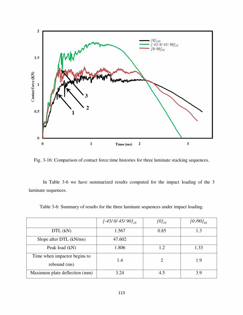
113
Fig. 3-16: Comparison of contact force time histories for three laminate stacking sequences.
In Table 3-6 we have summarized results computed for the impact loading of the 3
laminate sequences.
Table 3-6: Summary of results for the three laminate sequences under impact loading.
2S90] 45/ 0/ [-45/ 16[0] 4S/90] [0
DTL (kN) 1.567 0.85 1.3
Slope after DTL (kN/ms) 47.602
Peak load (kN) 1.806 1.2 1.33
Time when impactor begins to
rebound (ms) 1.4 2 1.9
Maximum plate deflection (mm) 3.24 4.5 3.9

114
11.2.5. Mesh sensitivity analysis
To see how sensitive the results are to the FE mesh, we consider 3 element sizes namely
0.65 mm (mesh 1), 0.775 mm (mesh 2) and 0.96 mm (mesh 3); these dimensions are for
elements that are in close vicinity of the impactor. The maximum size of an element along the
outer edges of the lamina varies from 1 mm for mesh 1 to 1.25 mm for mesh 3, see Fig. 3-17.
This results in approximately 120,000 elements for mesh 1, 85,000 elements for mesh 2, and
70,000 elements for mesh 3. The regions having the coarse and the fine mesh are shown in Fig.
3-17. The contact force time history plots for the 2S/90] /45 /0 [-45 laminate for the three FE
meshes, shown in Fig. 3-18, suggest that the mesh size has only a marginal effect on the contact
force time history. Each of these FE meshes has only one element through the thickness of a ply.
Also even for the finest FE mesh the element aspect ratio is more than the ideal one. However,
results provide a qualitative information about various aspects of the problem, and are not
necessarily converged values of various parameters.
Fig. 3-17: A graded FE mesh used in the impact analysis of the composite laminate.

115
Fig. 3-18: Contact force time histories plot for three different FE meshes.
We have summarized in Table 3-7 results obtained with the three different FE meshes.
Table 3-7: Summary of results for the 2S/90] /45 /0 [-45 laminate obtained with three different
meshes.
Mesh 1 Mesh 2 Mesh 3
DTL (kN) 1.3 1.4 1.56
Slope after DTL (kN/ms) 47.66 47.63 47.6
Peak load (kN) 1.74 1.87 1.81
Time when the sphere begins
to rebound (ms) 1.42 1.395 1.4
Plate deflection (mm) 3.36 3.32 3.24
Final K. E. of impactor (J) 2.06 2.1 2.17
0
0.75
1.5
2.25
0 1 2 3
Co
nta
ct f
orc
e (K
N)
Time (ms)
Mesh 1
Mesh 2
Mesh 3
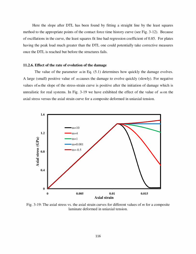
116
Here the slope after DTL has been found by fitting a straight line by the least squares
method to the appropriate points of the contact force time history curve (see Fig. 3-12). Because
of oscillations in the curve, the least squares fit line had regression coefficient of 0.85. For plates
having the peak load much greater than the DTL one could potentially take corrective measures
once the DTL is reached but before the structures fails.
11.2.6. Effect of the rate of evolution of the damage
The value of the parameter m in Eq. (5.1) determines how quickly the damage evolves.
A large (small) positive value of m causes the damage to evolve quickly (slowly). For negative
values of m the slope of the stress-strain curve is positive after the initiation of damage which is
unrealistic for real systems. In Fig. 3-19 we have exhibited the effect of the value of m on the
axial stress versus the axial strain curve for a composite deformed in uniaxial tension.
Fig. 3-19: The axial stress vs. the axial strain curves for different values of m for a composite
laminate deformed in uniaxial tension.
0
0.4
0.8
1.2
1.6
0 0.005 0.01 0.015
Axia
l st
ress
(G
Pa)
Axial strain
m=10
m=4
m=1
m=0.001
m=-0.5

117
Xiao et al. [16] have used 2=m for S2 glass/SC-15 epoxy composite and have
suggested tailoring the value of the parameter m based on experimental observations. Here we
have used the same value of m for all modes of damage. However, one intuitively expects that
the fiber damage would result in the immediate failure of the composite whereas the matrix
damage is more gradual and one should use a small value of m for it. In Fig. 3.20 we have
displayed time histories of the contact force for the 16 ply AS4/PEEK composite plate studied in
subsection 11.2.2.
Fig. 3-20: Comparison of the contact force time histories for m =4 and 100.
We have listed in Table 3-8 values of various quantities computed with m = 4 and 100.
0
0.6
1.2
1.8
0 1 2 3
Con
tact
forc
e (
KN
)
Time (ms)
m=4
m=100

118
Table 3-8: Summary of results for the 2S/90] /45 /0 [-45 laminate for m = 4 and 100.
m = 4 m = 100
DTL (kN) 1.567 1.4
Slope after DTL (kN/ms) 47.602 -
Peak load (kN) 1.806 1.48
Time when the sphere begins to
rebound (ms) 1.4 1.55
Maximum plate deflection (mm) 3.24 3.49
11.3. Effect of presence of the base plate on the response of the composite laminate
Since the composite laminate simply rests on the base plate, the laminate edges are lifted
from the plate during impact as should be clear from the fringe plots of the normal displacement
included in Fig. 3-21. The laminate points in yellow, brown and red regions have positive values
of u3 signifying that the back surface of the laminate in these regions is not contacting the
supporting steel plate.
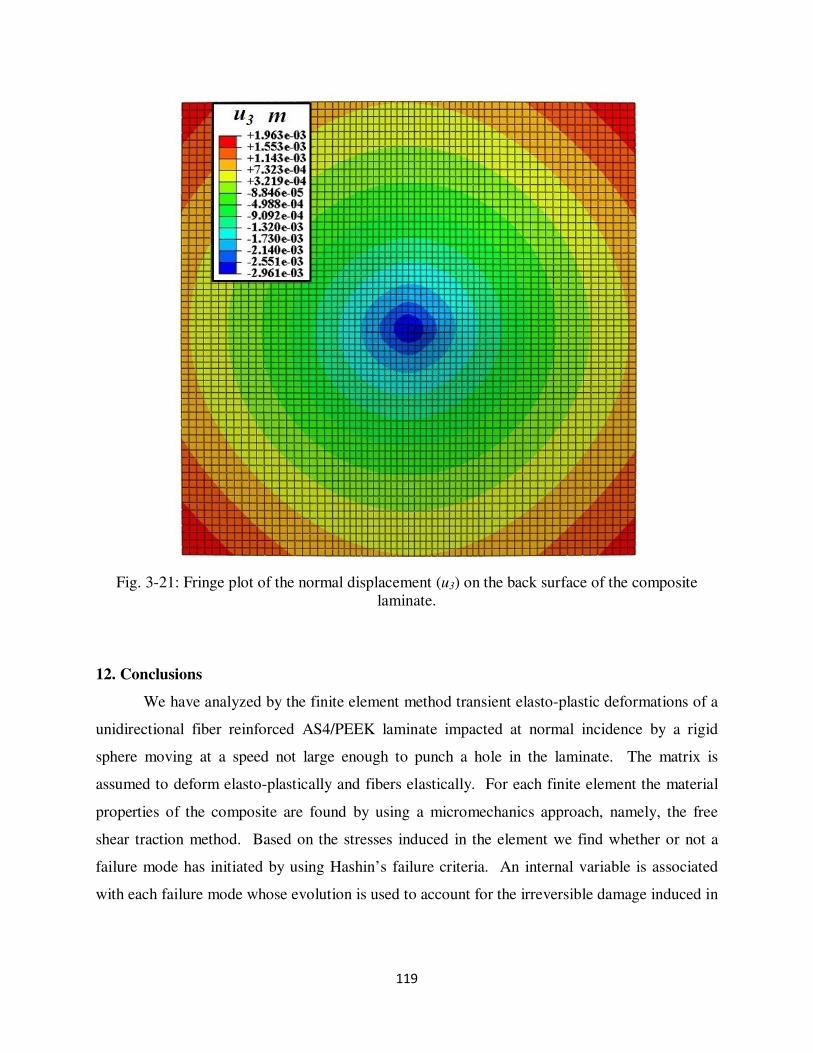
119
Fig. 3-21: Fringe plot of the normal displacement (u3) on the back surface of the composite
laminate.
12. Conclusions
We have analyzed by the finite element method transient elasto-plastic deformations of a
unidirectional fiber reinforced AS4/PEEK laminate impacted at normal incidence by a rigid
sphere moving at a speed not large enough to punch a hole in the laminate. The matrix is
assumed to deform elasto-plastically and fibers elastically. For each finite element the material
properties of the composite are found by using a micromechanics approach, namely, the free
shear traction method. Based on the stresses induced in the element we find whether or not a
failure mode has initiated by using Hashin’s failure criteria. An internal variable is associated
with each failure mode whose evolution is used to account for the irreversible damage induced in

120
the element. Thus values of material parameters of the constituents rather than those of the
composite are needed. However, values of strength parameters for the composite are required.
The computed time history of the total axial force acting on the impactor agrees well with
the experimental one available in the literature. For the problem studied the delamination failure
occurs over an extensive region beneath the spherical impactor. Fibers below the impactor fail in
compression, and the matrix in the bottom-most plies fails in tension. A wide crack develops in
the third ply from the bottom surface for the 2S/90] /45 /0 [-45 laminate. Results computed for
the three stacking sequences for the laminate suggest that the locations and the extent of the
failed regions strongly depend upon the stacking sequence. Also, the matrix may fail in tension
before fibers fail.
Acknowledgements:
This research was sponsored by the Army Research Laboratory and was accomplished under
Cooperative Agreement Number W911NF-06-2-0014. The views and conclusions contained in
this document are those of the authors and should not be interpreted as representing official
policies, either expressed or implied, of the Army Research Laboratory or the U.S. Government.
The U.S. Government is authorized to reproduce and distribute reprints for Government purposes
notwithstanding any copyright notation hereon. The work was also partially supported by the
Office of Naval Research Grant N00014-1-06-0567 to Virginia Polytechnic Institute and State
University with Dr. Y.D.S. Rajapakse as the program manager. Views expressed herein are
those of the authors and neither of the funding agencies nor their institutions.
References
1 Soden P. D., Kaddour A. S., Hinton, M. J., Recommendations for designers and
researchers resulting from the world-wide failure exercise. Composites Science and
Technology, 64, 2004, 589-601.
2 Togho K., Weng G. J., A progressive damage mechanics in particle-reinforced metal-
matrix composites under high tri-axial tension. Journal of Engineering Materials and
Technology, 116, 1994, 414-420.
3 Sun L. Z., Ju J. W., Liu H. T., Elasto-plastic modeling of metal matrix composites

121
with evolutionary particle de-bonding. Mechanics of Materials, 35, 2003, 559–569.
4 Nguyen B. N., Tucker B. J., Khaleel M. A., A mechanistic approach to matrix cracking
coupled with fiber-matrix de-bonding in short fiber reinforced composites. Journal of
engineering materials and technology, 127, 2005, 337-350.
5 Meraghni F., Blakeman C. J., Benzeggah M. L., Effect of interfacial decohesion on
stiffness reduction in a random discontinuous-fiber composite containing matrix micro-
cracks. Composites science and Technology, 56 , 1996, 541-555
6 Desrumaux F., Meraghni F., Benzeggah M. L., Micromechanical modeling coupled to a
reliability approach for damage evolution prediction in composite materials. Applied
composite materials, 7, 2000, 231-250.
7 Coleman B. D., Gurtin M., Thermodynamics with internal variables. Journal of Chemical
Physics, 47, 1967, 597-613.
8 Ladeveze P., Dantec E. Le., Damage modeling of the elementary ply for laminated
composites. Composites Science and Technology, 43, 1992, 257-267.
9 Hassan N. M., Batra R. C., Modeling damage in polymeric composites. Composites B, 39,
2008, 66–82.
10 Puck A., Schurmann H., Failure analysis of FRP laminates by means of physically based
phenomenological models. Composite Science and Technologies, 62, 2002, 1633-1662.
11 Hashin Z., Failure criteria for unidirectional fiber composites. Journal of Applied
Mechanics, 47, 1980, 329–334.
12 Donadon M. V., De .Almeida S. F. M, Arbelo M. A., Faria A. R.. Three-dimensional ply
failure model for composite Structures. International Journal of Aerospace Engineering,
2009, 2009, 1-22.
13 Clegg R. A., White D. M., Riedelb W., Harwick W. Hypervelocity impact damage
prediction in composites: Part I—material model and characterization. International
Journal of Impact Engineering, 33, 2006, 190–200.
14 Maa R.H., Cheng J. H., A CDM-based failure model for predicting strength of notched
composite laminates. Composites B, 33, 2002, 479–489.
15 Matzenmiller A., Lubliner J., Taylor R. L., A constitutive model for anisotropic damage in
fiber composites. Mechanics of Materials, 20, 1995, 125-152.
16 Xiao J. R., Gama B. A., Gillspie J. W., Progressive damage and delamination in plain
weave S-2 glass/SC-15 composites under quasi-static punch shear loading. Composites
Structures, 78, 2007, 182-196.
122
17 Williams K. V., Vaziri R., Application of a damage mechanics model for predicting the
impact response of composite materials. Composites and Structures, 79, 2001, 997-1011.
18 Robertson D. D., Mall S., Micromechanical analysis for thermo-viscoplastic behavior of
unidirectional fibrous composites. Composites Science and Technology, 50, 1994, 483-
496.
19 Aboudi J., Mechanics of composite materials. Elsevier science publication, Amsterdam ,
1991.
20 Curson A. D., Leach D. C., Moore D. R., Impact failure mechanisms in carbon
Fiber/PEEK composites. Journal of thermoplastic composite materials, 3, 1990, 24-31.
21 Weeks C. A., Sun C. T., Modeling non-linear rate-dependent behavior in fiber-reinforced
composites. Composite Science and Technology, 58, 1998, 603–11.
22 MAT 162 user reference manual, 2005
http://www.ccm.udel.edu/Tech/MAT162/MAT162Manual_v3.pdf
23 Benzeggah M. L., Kenane M., Measurement of mixed-mode delamination fracture
toughness of unidirectional glass/epoxy composites with mixed-mode bending apparatus.
Composites Science and Technology, 56, 1996, 439–449.
24 Raghava R. S., Caddell R. M., Yield locus studies of oriented polycarbonate: An
anisotropic and pressure-dependent solid. International Journal of Mechanical Sciences,
16, 1974, 789-792.
25 Gardner J. P., Micromechanical modeling of composite materials in finite element analysis
using an embedded cell approach. M.Sc. thesis, MIT, Cambridge, Massachusetts, 1994.
26 Chen J. K., Allahdadi F. A., Sun C. T., A quadratic yield function for fiber-reinforced
composites. Journal of composite materials, 31, 1997, 788-811.
27 Goldberg R. K., Stouffer D. C., Strain rate dependent analysis of a polymer matrix
composite utilizing a micromechanics approach. Journal of composite materials, 36, 2002,
773-793.
28 Kyriakides S., Arseculeratne R., Perry E., Liechti K., On the compressive failure of fiber
reinforced composites. International Journal of Solids and Structures, 32,1995, 689–738.
29 Chan S., Fawaz Z., Behdinan K., Amid R., Ballistic limit prediction using a numerical
model with progressive damage capability. Composite Structures, 77, 2007, 466–474.
30 Bordonaro C.M., Rate dependent mechanical behavior of high strength plastics:
experiment and modeling. PhD Dissertation, Rensselaer Polytechnic Institute, Troy, New

123
York, 1995.
31 Turon A., Da´vila C.G., Camanho P.P., Costa J., An engineering solution for mesh size
effects in the simulation of delamination using cohesive zone models. Engineering
Fracture Mechanics, 74, 2007, 1665-1682.
32 Schoeppner G. A., Abrate S., Delamination threshold loads for low velocity impact on
composite laminates. Composites A, 31, 2000, 903–915
33 Hitchens S. A., Kemp R. M. J., The effect of stacking sequence on impact damage in a
carbon fiber/epoxy composite. Composites, 26, 1995, 207-214.
34 Dorey G., Failure mode of composite materials with organic matrices and their
consequences in design. AGARD CP 163, 1975.
35 Fischer-Cripps A. C., Introduction to contact mechanics. Springer Science publication,
New York, 2010
36 ABAQUS 6.10 theory manual, http://www.esm.vt.edu/v6.10/
124
CHAPTER 4: Conclusions and Contributions
1. Conclusions
We have used four micromechanical theories, namely, the Mori-Tanaka, Eshelby’s
equivalent inclusion, the free shear traction method, and Hill’s equivalent energy principle, to
find values of material parameters for elasto-plastic deformations of AS4/PEEK composite. The
elasto-plastic deformations of the matrix are modeled by two yield criteria - the pressure-
independent von Mises and the pressure-dependent Drucker-Prager. Whereas the von Mises
yield surface is quadratic in deviatoric stresses the Drucker-Prager also has a linear term in the
hydrostatic pressure.
It is found that for fiber volume fraction, fv , varying from 0.3 to 0.6 the four micro-
mechanics approaches provide noticeably different values of the elastic moduli. For 6.0v =f ,
none of the four theories give values of all five elastic parameters that are close to the
experimental results available in the literature. We note that the difference in the minimum and
the maximum values of Young’s modulus in the direction transverse to fibers found
experimentally by three research groups equals 20%. Along the fibers, all four theories give
values of Young’s modulus that are very close to each other, and it can also be found by using
the rule of mixtures. When displacements are applied on all surfaces of a representative volume
element to produce a state of simple shear in the lamina plane, the value of the in-plane shear
modulus deduced from Hill’s equivalence energy principle is significantly higher than that
provided by the other three micromechanics approaches as well as the literature experimental
value.
For uniaxial elasto-plastic deformations of the composite lamina with fibers making an
angleθ with the axis of loading, the effective stress versus the effective plastic strain curves
computed with the von Mises yield criterion for the PEEK agree better with the experimental
results of Weeks and Sun than those derived by assuming that the yield criterion is pressure
dependent. Assuming that plastic deformations of the composite are also independent of the
hydrostatic pressure, we have found values, as a function of the volume fraction of fibers, of the
two material parameters in the yield surface and of the two material parameters that characterize
the strain dependent yield stress of the composite.

125
The pressure independent yield surface for the AS4/PEEK composite studied herein is
given by
( )
+== p
ij eln NAσ3Fσ where
( ) ( ) ( )[ ]212
21312
22323
23322ij σσ2Aσ2Aσσ
2
1σF +++−=
A = 2.597(VF)3
- 1.473(VF)2
+ 0.116(VF) + 0.396
N = 0.107(VF)3
+ 0.008(VF)2
- 0.050(VF) + 0.039
A23 = 158.0(VF)3
- 164.4(VF)2
+ 58.44(VF) - 1.5
A12 = 135.8(VF)3
- 138.8(VF)2
+ 47.77(VF) - 0.5
and VF equals the volume fraction of the fibers between 0.3 and 0.75, and values of A and N are
in MPa. By following a procedure similar to that used here and simulating homogeneous
deformations of the unidirectional fiber reinforced polymeric composite (UFPC) at different
strain rates, one can quantify the dependence of the yield stress of the UFPC upon the strain rate
characteristics of the fiber and the matrix.
We have also analyzed by the finite element method transient elasto-plastic deformations
of a unidirectional fiber reinforced AS4/PEEK laminate impacted at normal incidence by a rigid
sphere moving at a speed not large enough to punch a hole in the laminate. The matrix is
assumed to deform elasto-plastically and fibers elastically. For each finite element the material
properties of the composite are found by using a micromechanics approach, namely, the free
shear traction method. Based on the stresses induced in the element we find whether or not a
failure mode has initiated by using Hashin’s failure criteria. An internal variable is associated
with each failure mode whose evolution is used to account for the irreversible damage induced in
the element. Thus values of material parameters of the constituents rather than those of the
composite are needed. However, values of strength parameters for the composite are required.
The computed time history of the total axial force acting on the impactor agrees well with
the experimental one available in the literature. For the problem studied the delamination failure
occurs over an extensive region beneath the spherical impactor. Fibers below the impactor fail in

126
compression, and the matrix in the bottom-most plies fails in tension. A wide crack develops in
the third ply from the bottom surface for the 2S/90] /45 /0 [-45 laminate.
2. Contributions
A micromechanical analysis which uses constituent level properties to establish the
overall response of a heterogeneous material is computationally intensive, implying that it is
ideally suited to analyze simple problems under ideal loading conditions. One of the main
accomplishments of this work is to show the use of a micromechanics method for solving
realistic problems where there is non-uniform loading, e.g., impact problems, while considering
failure and damage during the loading process. Contributions of this work are summarized
below.
1. The free shear traction method for finding material properties of the lamina from those of its
constituents has been integrated with the finite element scheme to solve realistic problems
involving non-uniformly distributed loads. Thus only constituent level properties are needed for
the analysis. However, values of strength parameters for the lamina and those of parameters
appearing in the delamination criterion are also required for studying damage and failure.
2. A user defined subroutine has been developed to analyze damage and failure for 3-
dimensional problems, and has been integrated with the commercial FE software, ABAQUS.
3. The software has been used to analyze impact at normal incidence of a composite laminate by
a rigid sphere while considering various damage modes.

127
Appendix A ABAQUS input file for the impact analysis of UFPC laminate c*********************************************************************** *Heading
** Job name: AS4-PEEK Model name: Model-1
** Generated by: Abaqus/CAE Version 6.8-2
*Preprint, echo=NO, model=NO, history=NO, contact=NO ** ----------------------------------------------------------------
**
** PART INSTANCE: LAY1-ANG45N
**
*Node 1, 0.0500000007, 0., 0.000125000006
2, 0.0500000007, 0., 0.
---------------------------------------------------------
8843, 0.0269230772, 0.0237499997, 0.000125000006 8844, 0.0259615388, 0.0237499997, 0.000125000006
-----------------------------------------------------------
*Element, type=C3D8R
1, 146, 166, 1394, 1033, 1, 2, 33, 70 2, 1033, 1394, 1395, 1034, 70, 33, 34, 69
---------------------------------------------------------
4290, 858, 785, 20, 19, 8369, 8844, 646, 590
---------------------------------------------------------- ** Section: AS4-PEEK-SECTION
*Solid Section, elset=LAY1-ANG45N__PickedSet19, material=AS4-PEEK
-----------------------------------------------------------------
*Surface, type=ELEMENT, name=CONTACT-FORCE _CONTACT-FORCE_SPOS, SPOS
*Rigid Body, ref node=SPHERE-1-RefPt_, elset=SPHERE-1
**
** MATERIALS
** *Material, name=AS4-PEEK
*Density
1500.,
*Depvar, delete=100 100,
*User Material, constants=14
2.34e+11, 1.4e+10, 1.4e+10, 2.76e+10, 2.76e+10, 5.5e+09, 0.2, 0.2
0.25, 4.0e+09, 0.35, 1.527E8, 1.386E7, 0.60 *Material, name=STEEL
*Density
8000.,
*Elastic 2.1e+11, 0.25
**
** INTERACTION PROPERTIES
** ************************************************************************
*SURFACE INTERACTION, name=COHESIVE-INTERACTION
*COHESIVE BEHAVIOR, ELIGIBILITY=ORIGINAL CONTACTS, TYPE=UNCOUPLED
1.0E15, 1.0E15, 1.0E15 *DAMAGE INITIATION, CRITERION=QUADS
80.0E6, 150.0E6, 150.0E6
*DAMAGE EVOLUTION,TYPE=ENERGY,MIXED MODE BEHAVIOR=BK,POWER=1.7
150, 500, 500
************************************************************************* *CONTACT CLEARANCE, NAME=ADJUST-CLEARANCE, ADJUST=YES, CLEARANCE=0.0
*Surface Interaction, name=SPHERE-PLATE
*Friction
0.25, *Surface Behavior, pressure-overclosure=HARD
**
** BOUNDARY CONDITIONS
** ** Name: CONSTRAIN Type: Displacement/Rotation
*Boundary
VELOCITY, 1, 1
VELOCITY, 2, 2
128
VELOCITY, 4, 4
VELOCITY, 5, 5
VELOCITY, 6, 6 ** Name: FIX-BASE Type: Symmetry/Antisymmetry/Encastre
*Boundary
FIX-BASE, PINNED
** ** PREDEFINED FIELDS
**
** Name: VELOCITY Type: Velocity
*Initial Conditions, type=VELOCITY VELOCITY, 1, 0.
VELOCITY, 2, 0.
VELOCITY, 3, -4.
** ** INTERACTIONS
**
** Interaction: PLATE-SPHERE
*Contact, op=NEW *Contact Inclusions, ALL EXTERIOR
*Contact property assignment
, , SPHERE-PLATE
**************************************************** *CONTACT CLEARANCE ASSIGNMENT
LAY2_ANG0-TOP, LAY1_ANG45N-BOT, ADJUST-CLEARANCE
LAY3_ANG45-TOP, LAY2_ANG0-BOT, ADJUST-CLEARANCE
LAY4_ANG90-TOP, LAY3_ANG45-BOT, ADJUST-CLEARANCE
LAY5_ANG45N-TOP, LAY4_ANG90-BOT, ADJUST-CLEARANCE LAY6_ANG0-TOP, LAY5_ANG45N-BOT, ADJUST-CLEARANCE
LAY7_ANG45-TOP, LAY6_ANG0-BOT, ADJUST-CLEARANCE
LAY8_ANG90-TOP, LAY7_ANG45-BOT, ADJUST-CLEARANCE
LAY9_ANG90-TOP, LAY8_ANG90-BOT, ADJUST-CLEARANCE LAY10_ANG45-TOP, LAY9_ANG90-BOT, ADJUST-CLEARANCE
LAY11_ANG0-TOP, LAY10_ANG45-BOT, ADJUST-CLEARANCE
LAY12_ANG45N-TOP, LAY11_ANG0-BOT, ADJUST-CLEARANCE
LAY13_ANG90-TOP, LAY12_ANG45N-BOT, ADJUST-CLEARANCE LAY14_ANG45-TOP, LAY13_ANG90-BOT, ADJUST-CLEARANCE
LAY15_ANG0-TOP, LAY14_ANG45-BOT, ADJUST-CLEARANCE
LAY16_ANG45N-TOP, LAY15_ANG0-BOT, ADJUST-CLEARANCE
************************************************** ** ----------------------------------------------------------------
**
** STEP: IMPACT
** *Step, name=IMPACT, nlgeom = YES/NO
*Dynamic, Explicit, scale factor=0.45
, 0.004
*Bulk Viscosity
0.06, 1.2 **
** INTERACTIONS
**
** Interaction: PLATE-SPHERE ***********************************************************************************
*Contact, op=MOD
*CONTACT INCLUSIONS
LAY2_ANG0-TOP, LAY1_ANG45N-BOT LAY3_ANG45-TOP, LAY2_ANG0-BOT
LAY4_ANG90-TOP, LAY3_ANG45-BOT
LAY5_ANG45N-TOP, LAY4_ANG90-BOT
LAY6_ANG0-TOP, LAY5_ANG45N-BOT LAY7_ANG45-TOP, LAY6_ANG0-BOT
LAY8_ANG90-TOP, LAY7_ANG45-BOT
LAY9_ANG90-TOP, LAY8_ANG90-BOT
LAY10_ANG45-TOP, LAY9_ANG90-BOT LAY11_ANG0-TOP, LAY10_ANG45-BOT
LAY12_ANG45N-TOP, LAY11_ANG0-BOT
LAY13_ANG90-TOP, LAY12_ANG45N-BOT
LAY14_ANG45-TOP, LAY13_ANG90-BOT LAY15_ANG0-TOP, LAY14_ANG45-BOT
LAY16_ANG45N-TOP, LAY15_ANG0-BOT

129
**
*CONTACT PROPERTY ASSIGNMENT
LAY2_ANG0-TOP, LAY1_ANG45N-BOT,COHESIVE-INTERACTION LAY3_ANG45-TOP, LAY2_ANG0-BOT,COHESIVE-INTERACTION
LAY4_ANG90-TOP, LAY3_ANG45-BOT,COHESIVE-INTERACTION
LAY5_ANG45N-TOP, LAY4_ANG90-BOT,COHESIVE-INTERACTION
LAY6_ANG0-TOP, LAY5_ANG45N-BOT,COHESIVE-INTERACTION LAY7_ANG45-TOP, LAY6_ANG0-BOT,COHESIVE-INTERACTION
LAY8_ANG90-TOP, LAY7_ANG45-BOT,COHESIVE-INTERACTION
LAY9_ANG90-TOP, LAY8_ANG90-BOT,COHESIVE-INTERACTION
LAY10_ANG45-TOP, LAY9_ANG90-BOT,COHESIVE-INTERACTION LAY11_ANG0-TOP, LAY10_ANG45-BOT,COHESIVE-INTERACTION
LAY12_ANG45N-TOP, LAY11_ANG0-BOT,COHESIVE-INTERACTION
LAY13_ANG90-TOP, LAY12_ANG45N-BOT,COHESIVE-INTERACTION
LAY14_ANG45-TOP, LAY13_ANG90-BOT,COHESIVE-INTERACTION LAY15_ANG0-TOP, LAY14_ANG45-BOT,COHESIVE-INTERACTION
LAY16_ANG45N-TOP, LAY15_ANG0-BOT,COHESIVE-INTERACTION
*************************************************************************
** OUTPUT REQUESTS **
*Restart, write, number interval=1, time marks=NO
**
** FIELD OUTPUT: F-Output-1 **
*Output, field, number interval=250
*Node Output
RF, U, V
*Element Output, directions=YES E, S, SDV, STATUS
*Contact Output
CSDMG, CSQUADSCRT, CSTRESS
** ** HISTORY OUTPUT: H-Output-2
**
*Output, history, time interval=5e-06
*Contact Output, surface=CONTACT-FORCE CFN3, CFNM
**
** HISTORY OUTPUT: H-Output-1
** *Node Output, nset=VELOCITY
U3, V3
*End Step
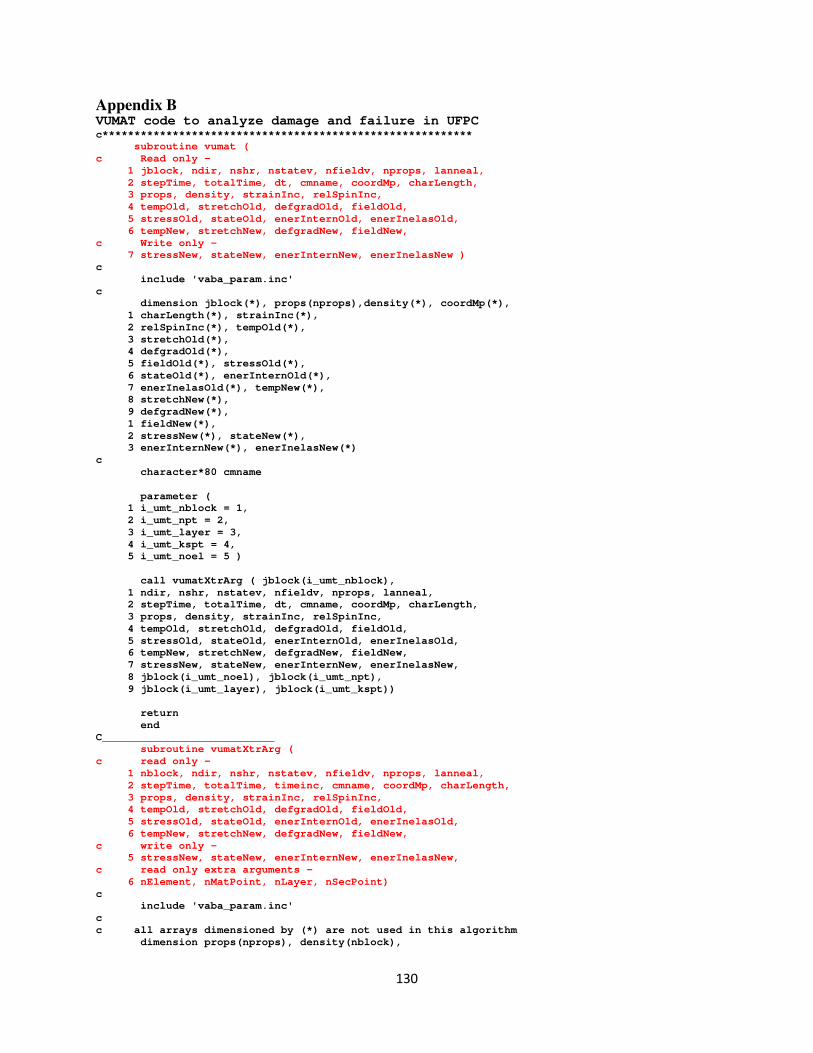
130
Appendix B VUMAT code to analyze damage and failure in UFPC c********************************************************** subroutine vumat (
c Read only -
1 jblock, ndir, nshr, nstatev, nfieldv, nprops, lanneal,
2 stepTime, totalTime, dt, cmname, coordMp, charLength, 3 props, density, strainInc, relSpinInc,
4 tempOld, stretchOld, defgradOld, fieldOld,
5 stressOld, stateOld, enerInternOld, enerInelasOld,
6 tempNew, stretchNew, defgradNew, fieldNew,
c Write only - 7 stressNew, stateNew, enerInternNew, enerInelasNew )
c
include 'vaba_param.inc'
c dimension jblock(*), props(nprops),density(*), coordMp(*),
1 charLength(*), strainInc(*),
2 relSpinInc(*), tempOld(*),
3 stretchOld(*), 4 defgradOld(*),
5 fieldOld(*), stressOld(*),
6 stateOld(*), enerInternOld(*),
7 enerInelasOld(*), tempNew(*), 8 stretchNew(*),
9 defgradNew(*),
1 fieldNew(*),
2 stressNew(*), stateNew(*), 3 enerInternNew(*), enerInelasNew(*)
c
character*80 cmname
parameter ( 1 i_umt_nblock = 1,
2 i_umt_npt = 2,
3 i_umt_layer = 3,
4 i_umt_kspt = 4, 5 i_umt_noel = 5 )
call vumatXtrArg ( jblock(i_umt_nblock),
1 ndir, nshr, nstatev, nfieldv, nprops, lanneal, 2 stepTime, totalTime, dt, cmname, coordMp, charLength,
3 props, density, strainInc, relSpinInc,
4 tempOld, stretchOld, defgradOld, fieldOld,
5 stressOld, stateOld, enerInternOld, enerInelasOld, 6 tempNew, stretchNew, defgradNew, fieldNew,
7 stressNew, stateNew, enerInternNew, enerInelasNew,
8 jblock(i_umt_noel), jblock(i_umt_npt),
9 jblock(i_umt_layer), jblock(i_umt_kspt))
return
end
C___________________________ subroutine vumatXtrArg (
c read only -
1 nblock, ndir, nshr, nstatev, nfieldv, nprops, lanneal,
2 stepTime, totalTime, timeinc, cmname, coordMp, charLength,
3 props, density, strainInc, relSpinInc, 4 tempOld, stretchOld, defgradOld, fieldOld,
5 stressOld, stateOld, enerInternOld, enerInelasOld,
6 tempNew, stretchNew, defgradNew, fieldNew,
c write only - 5 stressNew, stateNew, enerInternNew, enerInelasNew,
c read only extra arguments -
6 nElement, nMatPoint, nLayer, nSecPoint)
c include 'vaba_param.inc'
c
c all arrays dimensioned by (*) are not used in this algorithm
dimension props(nprops), density(nblock),

131
1 strainInc(nblock,ndir+nshr),
2 relSpinInc(nblock,nshr), defgradOld(nblock,9),
4 stressOld(nblock,ndir+nshr), 5 stateOld(nblock,nstatev), enerInternOld(nblock),
6 enerInelasOld(nblock),
7 stretchNew(nblock,ndir+nshr), defgradNew(nblock,9),
8 stressNew(nblock,ndir+nshr)
dimension enerInelasNew(nblock),stateNew(nblock,nstatev),
1 enerInternNew(nblock)
dimension nElement(nblock),nMatPoint(nblock),nLayer(nblock), 1 nSecPoint(nblock)
character*80 cmname
DOUBLE PRECISION, PARAMETER :: PI = 3.141592653589793D0
DOUBLE PRECISION, PARAMETER :: TOL_SOLUTION = 1.0E-8 INTEGER, PARAMETER :: ITERATE_LOOP = 20
C
DOUBLE PRECISION, PARAMETER :: DAMAGE_TOL = 0.95
DOUBLE PRECISION, PARAMETER :: STRAIN_TOL = 0.15 DOUBLE PRECISION, PARAMETER :: TENSILE_STRAIN_LMT = 0.05
DOUBLE PRECISION, PARAMETER :: CMPRSS_VOL = 0.1
DOUBLE PRECISION, PARAMETER :: EXPAND_VOL = 4.0
C_____ELASTIC PROPERTIES OF THE FIBER________ DOUBLE PRECISION :: E11_FIB, E22_FIB, E33_FIB
DOUBLE PRECISION :: G12_FIB, G13_FIB, G23_FIB
DOUBLE PRECISION :: NU12_FIB, NU13_FIB, NU23_FIB,
1 NU21_FIB, NU31_FIB, NU32_FIB
C_____MATRIX PROPERTIES_____ DOUBLE PRECISION :: E_MAT, NU_MAT, A_plast, N_pow
C_____VOLUME FRACTION___
DOUBLE PRECISION :: Vm, Vf
DOUBLE PRECISION :: RVE_a, RVE_b, RVE_c C_____TRANSFORMATION MATRIX___
INTEGER, DIMENSION(500000)::ALONG_0, ALONG_90, ALONG_45, ALONG_45N
INTEGER :: LNTH_0, LNTH_90, LNTH_45, LNTH_45N
DOUBLE PRECISION :: TETA DOUBLE PRECISION, DIMENSION(6,6) :: ROT_1 , ROT_2 ,
1 INV_ROT_1, INV_ROT_2
C_____COMPLIANCE AND STIFFNESS MATRIX OF FIBER AND MATRIX___
DOUBLE PRECISION, DIMENSION(6,6) :: C_INC, C_MAT, S_INC, S_MAT C_____COEFFICIENT MATRIX FOR NORMAL STRAIN___
DOUBLE PRECISION, DIMENSION(8,8) :: COEFF_NORMAL, INV_COEFF_NORMAL
C_____VECTOR FOR NORMAL STRAIN AND RHS FOR SOLUTION______
DOUBLE PRECISION, DIMENSION(8,1) :: SOLUTION_NORMAL, 1
VECTOR_NORMAL_RHS
C_____COEFFICIENT MATRIX FOR SHEAR STRAIN___
DOUBLE PRECISION, DIMENSION(12,12) :: COEFF_SHEAR, INV_COEFF_SHEAR
C_____VECTOR FOR SHEAR STRAIN AND RHS FOR SOLUTION______ DOUBLE PRECISION, DIMENSION(12,1) :: SOLUTION_SHEAR,
1
VECTOR_SHEAR_RHS
C_____TOTAL SOLUTION____ DOUBLE PRECISION, DIMENSION(20) :: OLD_TOTALsol, NEW_TOTALsol,
1 DIFF_sol
C_____NORM TO CHECK FOR CONVERGENCE____
DOUBLE PRECISION :: NORM_DIFF, NORM_SOL C_____STRAIN VECTORS IN EACH PHASE_____
DOUBLE PRECISION, DIMENSION(6,1) ::OLDstrain_F,
1 OLDstrain_M1, OLDstrain_M2, OLDstrain_M3
DOUBLE PRECISION, DIMENSION(6,1) ::NEWstrain_F, 1 NEWstrain_M1, NEWstrain_M2, NEWstrain_M3
C_____STRESS VECTORS IN EACH PHASE_____
DOUBLE PRECISION, DIMENSION(6,1) ::OLDstress_F,
1 OLDstress_M1, OLDstress_M2, OLDstress_M3 DOUBLE PRECISION, DIMENSION(6,1) ::NEWstress_F,
1 NEWstress_M1, NEWstress_M2, NEWstress_M3
C_____PLASTIC STRAIN IN EACH PHASE_____
DOUBLE PRECISION, DIMENSION(6,1) ::OLDplastic_M1, OLDplastic_M2, 1 OLDplastic_M3
DOUBLE PRECISION, DIMENSION(6,1) ::NEWplastic_M1, NEWplastic_M2,

132
1 NEWplastic_M3
C_____EFFECTIVE PLASTIC STRAIN IN EACH PHASE_____
DOUBLE PRECISION :: YIELDfn_MAX_M1, YIELDfn_MAX_M2, YIELDfn_MAX_M3 C_____INCREMENTAL STRAINS IN EACH PHASE_____
DOUBLE PRECISION, DIMENSION(6,1) :: Dstrain_F, Dstrain_M1,
1 Dstrain_M2, Dstrain_M3, Dstrain_RVE
C_____INCREMENTAL PLASTIC STRAIN IN EACH PHASE____ DOUBLE PRECISION, DIMENSION(6,1) ::Dplastic_M1, Dplastic_M2,
1 Dplastic_M3
C_____STRESS AND STRAIN IN RVE_____
DOUBLE PRECISION, DIMENSION(6,1) :: STRESS_RVE, STRAIN_RVE C_____ENERGY DENSITY_______
DOUBLE PRECISION :: ENERGY_DENSITY
C_____ELEMENT NUMBER____
INTEGER :: ELEMENT_NO, LOGIC C_____DAMAGE RELATED PARAMETERS______
DOUBLE PRECISION, DIMENSION(6,1) :: DAMAGEold_VECT, DAMAGEnew_VECT
DOUBLE PRECISION, DIMENSION(6,1) :: DAMAGE_STRESS
DOUBLE PRECISION :: Rv1, Rv2, Rv3, Rv4, Rv5 DOUBLE PRECISION :: PHI_1,PHI_2,PHI_3,PHI_4,PHI_5
C_____VOLUME EXPANSION VARIABLES___
DOUBLE PRECISION, DIMENSION(3,3) :: F_GRAD
DOUBLE PRECISION :: DET_F1, DET_F2, DET_F3, DET_F DOUBLE PRECISION :: VOL_RATIO
C_____VARIABLES TO DEFINE LOOP____
INTEGER :: I, J, K, L, IFLAG, LOOP
C____STORAGE OF HISTORY VARIABLES ALL IN LOCAL C/S______
C____stateOld(1:6) = STRAIN_RVE C
C____stateOld(7:12) = OLDstrain_F
C____stateOld(13:18)= OLDstrain_M1
C____stateOld(19:24)= OLDstrain_M2 C____stateOld(25:30)= OLDstrain_M3
C
C____stateOld(31:36)= OLDstress_F
C____stateOld(37:42)= OLDstress_M1 C____stateOld(43:48)= OLDstress_M2
C____stateOld(49:54)= OLDstress_M3
C
C____stateOld(55:60)= OLDplastic_M1 C____stateOld(61:66)= OLDplastic_M2
C____stateOld(67:72)= OLDplastic_M3
C
C____stateOld(73) = YIELDfn_MAX_M1 C____stateOld(74) = YIELDfn_MAX_M2
C____stateOld(75) = YIELDfn_MAX_M3
C****************************************
C____stateOld(80:85)= DAMAGE VARIABLES
C____stateOld(86:90)= PHI's C____stateOld(91:95)= RV's
C____ELASTIC PROPERTIES OF FIBER_______
E11_FIB = PROPS(1)
E22_FIB = PROPS(2) E33_FIB = PROPS(3)
G12_FIB = PROPS(4)
G13_FIB = PROPS(5)
G23_FIB = PROPS(6) NU12_FIB = PROPS(7)
NU13_FIB = PROPS(8)
NU23_FIB = PROPS(9)
C____CALCULATED POISSONS RATIO OF FIBER___ NU21_FIB = NU12_FIB*(E22_FIB/E11_FIB)
NU31_FIB = NU13_FIB*(E33_FIB/E11_FIB)
NU32_FIB = NU23_FIB*(E33_FIB/E22_FIB)
C___PROPERTIES OF MATRIX____ E_MAT = PROPS(10)
NU_MAT = PROPS(11)
C A_plast = CONSTANT N_pow = SLOPE
A_plast = PROPS(12) N_pow = PROPS(13)
Vf = PROPS(14)

133
C____VOLUME FRACTION OF MATRIX____
Vm = 1-Vf
C____RVE DIMENSIONS_____ RVE_a = SQRT(Vf)
RVE_b = 1.0D0 - RVE_a
RVE_c = RVE_b
C___ELEMENT SETS ASSOCIATED WITH ROTATION MATRIX___ CALL ELEMENT_SET(ALONG_0, ALONG_90, ALONG_45, ALONG_45N,
1 LNTH_0, LNTH_90, LNTH_45, LNTH_45N)
C
C____COMPLIANCE MATRIX OF FIBER_____ CALL COMPLIANCE_TRANS(E11_FIB, E22_FIB, E33_FIB,
1 G12_FIB, G13_FIB, G23_FIB,
2 NU12_FIB, NU13_FIB, NU23_FIB, S_INC)
C_INC = S_INC CALL MATINV(C_INC,6,6,IFLAG)
C
C____COMPLIANCE MATRIX OF MATRIX___
CALL COMPLIANCE_ISO(E_MAT, NU_MAT, S_MAT) C_MAT = S_MAT
CALL MATINV(C_MAT,6,6,IFLAG)
C
C______COEFFICIENT MATRIX FOR NORMAL STRAINS_______ COEFF_NORMAL = 0.0D0
C_____ROW 1____
COEFF_NORMAL(1,1) = RVE_a
COEFF_NORMAL(1,3) = RVE_b
C_____ROW 2____ COEFF_NORMAL(2,5) = RVE_b
COEFF_NORMAL(2,7) = RVE_a
C_____ROW 3____
COEFF_NORMAL(3,2) = RVE_a COEFF_NORMAL(3,8) = RVE_c
C_____ROW 4____
COEFF_NORMAL(4,4) = RVE_a
COEFF_NORMAL(4,6) = RVE_c C_____ROW 5____
COEFF_NORMAL(5,1) = C_INC(2,2)
COEFF_NORMAL(5,2) = C_INC(2,3)
COEFF_NORMAL(5,3) = -C_MAT(2,2) COEFF_NORMAL(5,4) = -C_MAT(2,3)
C_____ROW 6____
COEFF_NORMAL(6,5) = C_MAT(2,2)
COEFF_NORMAL(6,6) = C_MAT(2,3) COEFF_NORMAL(6,7) =-C_MAT(2,2)
COEFF_NORMAL(6,8) =-C_MAT(2,3)
C_____ROW 7____
COEFF_NORMAL(7,1) = C_INC(3,2)
COEFF_NORMAL(7,2) = C_INC(3,3) COEFF_NORMAL(7,7) =-C_MAT(3,2)
COEFF_NORMAL(7,8) =-C_MAT(3,3)
C_____ROW 8____
COEFF_NORMAL(8,3) = C_MAT(3,2) COEFF_NORMAL(8,4) = C_MAT(3,3)
COEFF_NORMAL(8,5) =-C_MAT(3,2)
COEFF_NORMAL(8,6) =-C_MAT(3,3)
C___________________________________ INV_COEFF_NORMAL = COEFF_NORMAL
CALL MATINV(INV_COEFF_NORMAL,8,8,IFLAG)
C
C______COEFFICIENT MATRIX FOR SHEAR STRAINS_______ COEFF_SHEAR = 0.0D0
C_____ROW 1____
COEFF_SHEAR(1,3) = 1.0D0
COEFF_SHEAR(1,12) = -1.0D0 C_____ROW 2_____
COEFF_SHEAR(2,6) = 1.0D0
COEFF_SHEAR(2,9) = -1.0D0
C_____ROW 3_____ COEFF_SHEAR(3,3) = RVE_a
COEFF_SHEAR(3,6) = RVE_b

134
C_____ROW 4_____
COEFF_SHEAR(4,2) = 1.0D0
COEFF_SHEAR(4,5) = -1.0D0 C_____ROW 5____
COEFF_SHEAR(5,8) = 1.0D0
COEFF_SHEAR(5,11) = -1.0D0
C_____ROW 6____ COEFF_SHEAR(6,2) = RVE_a
COEFF_SHEAR(6,11) = RVE_c
C_____ROW 7____
COEFF_SHEAR(7,1) = RVE_a*RVE_a COEFF_SHEAR(7,4) = RVE_a*RVE_b
COEFF_SHEAR(7,7) = RVE_b*RVE_c
COEFF_SHEAR(7,10) = RVE_a*RVE_c
C_____ROW 8____ COEFF_SHEAR(8,3) = RVE_a*C_INC(6,6)
COEFF_SHEAR(8,6) = -RVE_a*C_MAT(6,6)
COEFF_SHEAR(8,9) = -RVE_c*C_MAT(6,6)
COEFF_SHEAR(8,12) = RVE_c*C_MAT(6,6) C_____ROW 9_____
COEFF_SHEAR(9,2) = RVE_a*C_INC(5,5)
COEFF_SHEAR(9,5) = RVE_b*C_MAT(5,5)
COEFF_SHEAR(9,8) = -RVE_b*C_MAT(5,5) COEFF_SHEAR(9,11) = -RVE_a*C_MAT(5,5)
C_____ROW 10____
COEFF_SHEAR(10,1) = C_INC(4,4)
COEFF_SHEAR(10,10)= -C_MAT(4,4)
C_____ROW 11____ COEFF_SHEAR(11,1) = C_INC(4,4)
COEFF_SHEAR(11,4) = -C_MAT(4,4)
C_____ROW 12____
COEFF_SHEAR(12,1) = C_INC(4,4) COEFF_SHEAR(12,7) = -C_MAT(4,4)
C___________________________________
INV_COEFF_SHEAR = COEFF_SHEAR
CALL MATINV(INV_COEFF_SHEAR,12,12,IFLAG) C
C*****MAKE COMPUTATIONS AT EVERY MATERIAL POINT********
DO KM = 1,nblock
LOGIC=0 ELEMENT_NO = nElement(KM)
C_________ASSIGN ANGLE TO EACH ELEMENT___
IF(LOGIC .EQ. 0)THEN
DO I = 1, LNTH_0 IF(ELEMENT_NO .EQ. ALONG_0(I))THEN
TETA =0.0
LOGIC=1
EXIT
END IF END DO
END IF
IF(LOGIC .EQ. 0)THEN
DO I = 1, LNTH_90 IF(ELEMENT_NO .EQ. ALONG_90(I))THEN
TETA = (1.0D0/2.0D0)*PI
LOGIC=1
EXIT END IF
END DO
END IF
IF(LOGIC .EQ. 0)THEN DO I = 1, LNTH_45
IF(ELEMENT_NO .EQ. ALONG_45(I))THEN
TETA = (1.0D0/4.0D0)*PI
LOGIC=1 EXIT
END IF
END DO
END IF IF(LOGIC .EQ. 0)THEN
DO I = 1, LNTH_45N
135
IF(ELEMENT_NO .EQ. ALONG_45N(I))THEN
TETA = -(1.0D0/4.0D0)*PI
LOGIC=1 EXIT
END IF
END DO
END IF CALL ROTATION(TETA, ROT_1, ROT_2, INV_ROT_1, INV_ROT_2)
C
C_________INCREMENTAL STRAIN IN GLOBAL COORDINATE SYSTEM______
Dstrain_RVE(1,1) = strainInc(KM,1) Dstrain_RVE(2,1) = strainInc(KM,2)
Dstrain_RVE(3,1) = strainInc(KM,3)
Dstrain_RVE(4,1) = 2.0D0*strainInc(KM,5)
Dstrain_RVE(5,1) = 2.0D0*strainInc(KM,6) Dstrain_RVE(6,1) = 2.0D0*strainInc(KM,4)
C_________ROTATE INCREMENTAL STRAIN TO LOCAL COORDINATE SYSTEM______
Dstrain_RVE = MATMUL(ROT_2, Dstrain_RVE)
C C_________stateOld(1:6) = STRAIN_RVE
C_________STRAIN IN RVE (LOCAL C/S): PRESENT TIME STEP_____
DO I=1,6
STRAIN_RVE(I,1) = stateOld(KM,I) + Dstrain_RVE(I,1) END DO
C_________stateOld(7:12) = OLDstrain_F
C_________stateOld(13:18) = OLDstrain_M1
C_________stateOld(19:24) = OLDstrain_M2
C_________stateOld(25:30) = OLDstrain_M3 DO I=1,6
OLDstrain_F(I,1) = stateOld(KM,I+6)
OLDstrain_M1(I,1)= stateOld(KM,I+12)
OLDstrain_M2(I,1)= stateOld(KM,I+18) OLDstrain_M3(I,1)= stateOld(KM,I+24)
END DO
C_________stateOld(31:36) = OLDstress_F
C_________stateOld(37:42) = OLDstress_M1 C_________stateOld(43:48) = OLDstress_M2
C_________stateOld(49:54) = OLDstress_M3
DO I=1,6
OLDstress_F(I,1) = stateOld(KM,I+30) OLDstress_M1(I,1)= stateOld(KM,I+36)
OLDstress_M2(I,1)= stateOld(KM,I+42)
OLDstress_M3(I,1)= stateOld(KM,I+48)
END DO C_________stateOld(55:60) = OLDplastic_M1
C_________stateOld(61:66) = OLDplastic_M2
C_________stateOld(67:72) = OLDplastic_M3
DO I=1,6
OLDplastic_M1(I,1) = stateOld(KM,I+54) OLDplastic_M2(I,1) = stateOld(KM,I+60)
OLDplastic_M3(I,1) = stateOld(KM,I+66)
END DO
C_________stateOld(73) = YIELDfn_MAX_M1 C_________stateOld(74) = YIELDfn_MAX_M2
C_________stateOld(75) = YIELDfn_MAX_M3
YIELDfn_MAX_M1 = stateOld(KM, 73)
YIELDfn_MAX_M2 = stateOld(KM, 74) YIELDfn_MAX_M3 = stateOld(KM, 75)
C_______START ITERATIVE LOOP FOR CONVERGENCE OF STRAINS_____
C________ASSUME INCRMENTAL PLASTIC STRAIN TO BE ZERO_______
Dplastic_M1 = 0.0D0 Dplastic_M2 = 0.0D0
Dplastic_M3 = 0.0D0
C_______INITIALIZE SOLUTION VECTOR TO BE ZERO_____
OLD_TOTALsol = 0.0D0 C______#####################################################################______
DO LOOP = 1, ITERATE_LOOP
C_________RHS VECTOR FOR NORMAL STRAINS_____
VECTOR_NORMAL_RHS = 0.0D0 C
VECTOR_NORMAL_RHS(1,1) = (RVE_a + RVE_b)*STRAIN_RVE(2,1)

136
C
VECTOR_NORMAL_RHS(2,1) = (RVE_a + RVE_b)*STRAIN_RVE(2,1)
C VECTOR_NORMAL_RHS(3,1) = (RVE_a + RVE_c)*STRAIN_RVE(3,1)
C
VECTOR_NORMAL_RHS(4,1) = (RVE_a + RVE_c)*STRAIN_RVE(3,1)
C VECTOR_NORMAL_RHS(5,1) = (C_MAT(2,1) - C_INC(2,1))*
1 STRAIN_RVE(1,1)
2 - C_MAT(2,1)*(OLDplastic_M1(1,1) + Dplastic_M1(1,1))
3 - C_MAT(2,2)*(OLDplastic_M1(2,1) + Dplastic_M1(2,1)) 4 - C_MAT(2,3)*(OLDplastic_M1(3,1) + Dplastic_M1(3,1))
C
VECTOR_NORMAL_RHS(6,1) =
1 C_MAT(2,1)*(OLDplastic_M2(1,1) + Dplastic_M2(1,1)) 2 - C_MAT(2,1)*(OLDplastic_M3(1,1) + Dplastic_M3(1,1))
3 + C_MAT(2,2)*(OLDplastic_M2(2,1) + Dplastic_M2(2,1))
4 - C_MAT(2,2)*(OLDplastic_M3(2,1) + Dplastic_M3(2,1))
5 + C_MAT(2,3)*(OLDplastic_M2(3,1) + Dplastic_M2(3,1)) 6 - C_MAT(2,3)*(OLDplastic_M3(3,1) + Dplastic_M3(3,1))
C
VECTOR_NORMAL_RHS(7,1) = (C_MAT(3,1) - C_INC(3,1))*
1 STRAIN_RVE(1,1) 2 - C_MAT(3,1)*(OLDplastic_M3(1,1) + Dplastic_M3(1,1))
3 - C_MAT(3,2)*(OLDplastic_M3(2,1) + Dplastic_M3(2,1))
4 - C_MAT(3,3)*(OLDplastic_M3(3,1) + Dplastic_M3(3,1))
C
VECTOR_NORMAL_RHS(8,1) = 1 C_MAT(3,1)*(OLDplastic_M1(1,1) + Dplastic_M1(1,1))
2 - C_MAT(3,1)*(OLDplastic_M2(1,1) + Dplastic_M2(1,1))
3 + C_MAT(3,2)*(OLDplastic_M1(2,1) + Dplastic_M1(2,1))
4 - C_MAT(3,2)*(OLDplastic_M2(2,1) + Dplastic_M2(2,1)) 5 + C_MAT(3,3)*(OLDplastic_M1(3,1) + Dplastic_M1(3,1))
6 - C_MAT(3,3)*(OLDplastic_M2(3,1) + Dplastic_M2(3,1))
C
C_________RHS VECTOR FOR SHEAR STRAINS_____ VECTOR_SHEAR_RHS = 0.0D0
C
VECTOR_SHEAR_RHS(1,1) = 0.0D0
C VECTOR_SHEAR_RHS(2,1) = 0.0D0
C
VECTOR_SHEAR_RHS(3,1) = (RVE_a + RVE_b)*STRAIN_RVE(6,1)
C VECTOR_SHEAR_RHS(4,1) = 0.0D0
C
VECTOR_SHEAR_RHS(5,1) = 0.0D0
C
VECTOR_SHEAR_RHS(6,1) = (RVE_a + RVE_c)*STRAIN_RVE(5,1) C
VECTOR_SHEAR_RHS(7,1) = (RVE_a + RVE_b)*
1 (RVE_a + RVE_c)*STRAIN_RVE(4,1)
C VECTOR_SHEAR_RHS(8,1) =
1 C_MAT(6,6)*RVE_c*(OLDplastic_M3(6,1) + Dplastic_M3(6,1))
2 - C_MAT(6,6)*RVE_a*(OLDplastic_M1(6,1) + Dplastic_M1(6,1))
3 - C_MAT(6,6)*RVE_c*(OLDplastic_M2(6,1) + Dplastic_M2(6,1)) C
VECTOR_SHEAR_RHS(9,1) =
1 C_MAT(5,5)*RVE_b*(OLDplastic_M1(5,1) + Dplastic_M1(5,1))
2 - C_MAT(5,5)*RVE_a*(OLDplastic_M3(5,1) + Dplastic_M3(5,1)) 3 - C_MAT(5,5)*RVE_b*(OLDplastic_M2(5,1) + Dplastic_M2(5,1))
C
VECTOR_SHEAR_RHS(10,1)=
1 - C_MAT(4,4)*(OLDplastic_M3(4,1) + Dplastic_M3(4,1)) C
VECTOR_SHEAR_RHS(11,1)=
1 - C_MAT(4,4)*(OLDplastic_M1(4,1) + Dplastic_M1(4,1))
C VECTOR_SHEAR_RHS(12,1)=
1 - C_MAT(4,4)*(OLDplastic_M2(4,1) + Dplastic_M2(4,1))

137
C
C________SOLUTION FOR NORMAL STRAINS___
SOLUTION_NORMAL = MATMUL(INV_COEFF_NORMAL,VECTOR_NORMAL_RHS) C
C________SOLUTION FOR SHEAR STRAINS___
SOLUTION_SHEAR = MATMUL(INV_COEFF_SHEAR,VECTOR_SHEAR_RHS)
C________STRAIN IN EACH PHASE___ C_______STRAIN IN FIBER____
NEWstrain_F(1,1) = STRAIN_RVE(1,1)
NEWstrain_F(2,1) = SOLUTION_NORMAL(1,1)
NEWstrain_F(3,1) = SOLUTION_NORMAL(2,1) C
NEWstrain_F(4,1) = SOLUTION_SHEAR(1,1)
NEWstrain_F(5,1) = SOLUTION_SHEAR(2,1)
NEWstrain_F(6,1) = SOLUTION_SHEAR(3,1) C_______STRAIN IN MATRIX: M1____
NEWstrain_M1(1,1) = STRAIN_RVE(1,1)
NEWstrain_M1(2,1) = SOLUTION_NORMAL(3,1)
NEWstrain_M1(3,1) = SOLUTION_NORMAL(4,1) C
NEWstrain_M1(4,1) = SOLUTION_SHEAR(4,1)
NEWstrain_M1(5,1) = SOLUTION_SHEAR(5,1)
NEWstrain_M1(6,1) = SOLUTION_SHEAR(6,1) C_______STRAIN IN MATRIX: M2____
NEWstrain_M2(1,1) = STRAIN_RVE(1,1)
NEWstrain_M2(2,1) = SOLUTION_NORMAL(5,1)
NEWstrain_M2(3,1) = SOLUTION_NORMAL(6,1)
C NEWstrain_M2(4,1) = SOLUTION_SHEAR(7,1)
NEWstrain_M2(5,1) = SOLUTION_SHEAR(8,1)
NEWstrain_M2(6,1) = SOLUTION_SHEAR(9,1)
C_______STRAIN IN MATRIX: M3____ NEWstrain_M3(1,1) = STRAIN_RVE(1,1)
NEWstrain_M3(2,1) = SOLUTION_NORMAL(7,1)
NEWstrain_M3(3,1) = SOLUTION_NORMAL(8,1)
C NEWstrain_M3(4,1) = SOLUTION_SHEAR(10,1)
NEWstrain_M3(5,1) = SOLUTION_SHEAR(11,1)
NEWstrain_M3(6,1) = SOLUTION_SHEAR(12,1)
C C________INCREMENTAL STRAINS IN EACH PHASE______
Dstrain_F = NEWstrain_F - OLDstrain_F
Dstrain_M1 = NEWstrain_M1 - OLDstrain_M1
Dstrain_M2 = NEWstrain_M2 - OLDstrain_M2 Dstrain_M3 = NEWstrain_M3 - OLDstrain_M3
C________TOTAL SOLUTION__
DO I = 1, 8
NEW_TOTALsol(I) = SOLUTION_NORMAL(I,1) END DO
DO I = 1, 12
NEW_TOTALsol(I+8) = SOLUTION_SHEAR(I,1)
END DO C
DIFF_SOL = NEW_TOTALsol - OLD_TOTALsol
C
C________NORM OF SOLUTION VECTORS TO CHECK FOR CONVERGENCE______ NORM_SOL = DOT_PRODUCT(NEW_TOTALsol, NEW_TOTALsol)
NORM_SOL = SQRT(NORM_SOL)
NORM_DIFF = DOT_PRODUCT(DIFF_SOL, DIFF_SOL)
NORM_DIFF = SQRT(NORM_DIFF) IF(NORM_SOL .EQ. 0.0D0)NORM_SOL = 1.0D0
IF(ABS(NORM_DIFF/NORM_SOL) .LE. TOL_SOLUTION)EXIT
OLD_TOTALsol = NEW_TOTALsol
C________CALL PLASTIC ROUTINE TO CHECK FOR INELASTIC DEFORMATION______ C________PLASTIC DEFORMATION: M1______
CALL PLASTIC (C_MAT, A_plast, N_pow, YIELDfn_MAX_M1,
1 Dstrain_M1, OLDstress_M1, NEWstress_M1,
2 OLDstrain_M1, NEWstrain_M1, OLDplastic_M1, NEWplastic_M1, 3 Dplastic_M1, totalTime, timeinc)

138
C________PLASTIC DEFORMATION: M2______
CALL PLASTIC (C_MAT, A_plast, N_pow, YIELDfn_MAX_M2,
1 Dstrain_M2, OLDstress_M2, NEWstress_M2, 2 OLDstrain_M2, NEWstrain_M2, OLDplastic_M2, NEWplastic_M2,
3 Dplastic_M2, totalTime, timeinc)
C________PLASTIC DEFORMATION: M3______
CALL PLASTIC (C_MAT, A_plast, N_pow, YIELDfn_MAX_M3, 1 Dstrain_M3, OLDstress_M3, NEWstress_M3,
2 OLDstrain_M3, NEWstrain_M3, OLDplastic_M3, NEWplastic_M3,
3 Dplastic_M3, totalTime, timeinc)
C END DO
C______#####################################################################______
C________STRESS IN EACH PHASE___
C________STRESS IN FIBER____ NEWstress_F = MATMUL(C_INC, NEWstrain_F)
C_______STRESS IN M1, M2 & M3 CALCULATED FROM PLASTICITY ROUTINE________
C
C________STRESS IN RVE____ STRESS_RVE(1,1) = RVE_a*RVE_a*NEWstress_F(1,1)
1 + RVE_a*RVE_b*NEWstress_M1(1,1)
2 + RVE_b*RVE_c*NEWstress_M2(1,1)
3 + RVE_a*RVE_c*NEWstress_M3(1,1) STRESS_RVE(1,1) = STRESS_RVE(1,1)/(RVE_a + RVE_b)
STRESS_RVE(1,1) = STRESS_RVE(1,1)/(RVE_a + RVE_c)
C
STRESS_RVE(2,1) = RVE_a*NEWstress_M1(2,1)
1 + RVE_c*NEWstress_M2(2,1) STRESS_RVE(2,1) = STRESS_RVE(2,1)/(RVE_a + RVE_c)
C
STRESS_RVE(3,1) = RVE_a*NEWstress_M3(3,1)
1 + RVE_b*NEWstress_M2(3,1) STRESS_RVE(3,1) = STRESS_RVE(3,1)/(RVE_a + RVE_b)
C
STRESS_RVE(4,1) = NEWstress_F(4,1)
C STRESS_RVE(5,1) = RVE_a*NEWstress_F(5,1)
1 + RVE_b*NEWstress_M1(5,1)
STRESS_RVE(5,1) = STRESS_RVE(5,1)/(RVE_a + RVE_b)
C STRESS_RVE(6,1) = RVE_a*NEWstress_F(6,1)
1 + RVE_c*NEWstress_M3(6,1)
STRESS_RVE(6,1) = STRESS_RVE(6,1)/(RVE_a + RVE_c)
C C_________STORAGE OF DAMAGE HISTORY VARIABLES______
C_________stateOld(100) = DELETION
C_________stateOld(80:85) = DAMAGE VARIABLES
C_________stateOld(86:90) = PHI's
C_________stateOld(91:95) = RV's DO I=1,6
DAMAGEold_VECT(I,1)= stateOld(KM,79+I)
END DO
C________INITIALIZE VISUALIZING VARIABLES_______ PHI_1 = stateOld(KM,86)
PHI_2 = stateOld(KM,87)
PHI_3 = stateOld(KM,88)
PHI_4 = stateOld(KM,89) PHI_5 = stateOld(KM,90)
Rv1 = stateOld(KM,91)
Rv2 = stateOld(KM,92)
RV3 = stateOld(KM,93) RV4 = stateOld(KM,94)
RV5 = stateOld(KM,95)
C_________CALL DAMAGE SUBROUTINE____
CALL HASHIN_DAMAGE(STRESS_RVE, DAMAGEold_VECT, DAMAGEnew_VECT, 1 Rv1, Rv2, Rv3, Rv4, Rv5, PHI_1, PHI_2, PHI_3, PHI_4, PHI_5)
C________DAMAGED STRESS_____
DAMAGE_STRESS(1,1)=(1.0-DAMAGEnew_VECT(1,1))*STRESS_RVE(1,1)
DAMAGE_STRESS(2,1)=(1.0-DAMAGEnew_VECT(2,1))*STRESS_RVE(2,1) DAMAGE_STRESS(3,1)=(1.0-DAMAGEnew_VECT(3,1))*STRESS_RVE(3,1)
DAMAGE_STRESS(4,1)=(1.0-DAMAGEnew_VECT(4,1))*STRESS_RVE(4,1)

139
DAMAGE_STRESS(5,1)=(1.0-DAMAGEnew_VECT(5,1))*STRESS_RVE(5,1)
DAMAGE_STRESS(6,1)=(1.0-DAMAGEnew_VECT(6,1))*STRESS_RVE(6,1)
C_________UPDATE HISTORY VARIABLES IN L/C SYSTEM______ C_________stateNew(1:6) = STRAIN_RVE
DO I=1,6
stateNew(KM, I) = STRAIN_RVE(I,1)
END DO C_________stateNew(7:12) = NEWstrain_F
C_________stateNew(13:18) = NEWstrain_M1
C_________stateNew(19:24) = NEWstrain_M2
C_________stateNew(25:30) = NEWstrain_M3 DO I=1,6
stateNEW(KM,I+6) = NEWstrain_F(I,1)
stateNEW(KM,I+12) = NEWstrain_M1(I,1)
stateNEW(KM,I+18) = NEWstrain_M2(I,1) stateNEW(KM,I+24) = NEWstrain_M3(I,1)
END DO
C_________stateNew(31:36) = NEWstress_F
C_________stateNew(37:42) = NEWstress_M1 C_________stateNew(43:48) = NEWstress_M2
C_________stateNew(49:54) = NEWstress_M3
DO I=1,6
stateNEW(KM,I+30) = NEWstress_F(I,1) stateNEW(KM,I+36) = NEWstress_M1(I,1)
stateNEW(KM,I+42) = NEWstress_M2(I,1)
stateNEW(KM,I+48) = NEWstress_M3(I,1)
END DO
C_________stateNew(55:60) = NEWplastic_M1 C_________stateNew(61:66) = NEWplastic_M2
C_________stateNew(67:72) = NEWplastic_M3
DO I=1,6
stateNEW(KM,I+54) = NEWplastic_M1(I,1) stateNEW(KM,I+60) = NEWplastic_M2(I,1)
stateNEW(KM,I+66) = NEWplastic_M3(I,1)
END DO
C_________stateNew(73) = YIELDfn_MAX_M1 C_________stateNew(74) = YIELDfn_MAX_M2
C_________stateNew(75) = YIELDfn_MAX_M3
stateNew(KM, 73) = YIELDfn_MAX_M1
stateNew(KM, 74) = YIELDfn_MAX_M2 stateNew(KM, 75) = YIELDfn_MAX_M3
C_________STORAGE OF DAMAGE HISTORY VARIABLES______
C_________stateOld(80:85) = DAMAGE VARIABLES
C_________stateOld(86:90) = PHI's C________UPDATE DAMAGE VARIABLES______
DO I=1,6
stateNew(KM,79+I)=DAMAGEnew_VECT(I,1)
END DO
C________UPDATE DAMAGE VISUALIZATION VARIABLES_______ stateNew(KM,86) = PHI_1
stateNew(KM,87) = PHI_2
stateNew(KM,88) = PHI_3
stateNew(KM,89) = PHI_4 stateNew(KM,90) = PHI_5
stateNew(KM,91) = RV1
stateNew(KM,92) = RV2
stateNew(KM,93) = RV3 stateNew(KM,94) = RV4
stateNew(KM,95) = RV5
C____________ROTATE STRESS BACK TO GLOBAL COORDINATE SYSTEM_____
DAMAGE_STRESS = MATMUL(INV_ROT_1, DAMAGE_STRESS) C
stressNew(KM, 1) = DAMAGE_STRESS(1,1)
stressNew(KM, 2) = DAMAGE_STRESS(2,1)
stressNew(KM, 3) = DAMAGE_STRESS(3,1) stressNew(KM, 4) = DAMAGE_STRESS(6,1)
stressNew(KM, 5) = DAMAGE_STRESS(4,1)
stressNew(KM, 6) = DAMAGE_STRESS(5,1)
C____ENERGY UPDATE_____ ENERGY_DENSITY = 0.5D0*(
1 (stressOld(KM,1) + stressNew(KM,1))*strainInc(KM,1)

140
2 + (stressOld(KM,2) + stressNew(KM,2))*strainInc(KM,2)
3 + (stressOld(KM,3) + stressNew(KM,3))*strainInc(KM,3)
4 + 2.0D0*(stressOld(KM,4) + stressNew(KM,4))*strainInc(KM,4) 5 + 2.0D0*(stressOld(KM,5) + stressNew(KM,5))*strainInc(KM,5)
6 + 2.0D0*(stressOld(KM,6) + stressNew(KM,6))*strainInc(KM,6))
C
enerInternNew(KM) = enerInternOld(KM) + 1 ENERGY_DENSITY/density(KM)
C
C________VOLUMETRIC STRAIN_____
F_GRAD(1,1)= defgradNew(KM,1) F_GRAD(1,2)= defgradNew(KM,4)
F_GRAD(1,3)= defgradNew(KM,9)
C
F_GRAD(2,1)= defgradNew(KM,7) F_GRAD(2,2)= defgradNew(KM,2)
F_GRAD(2,3)= defgradNew(KM,5)
C
F_GRAD(3,1)= defgradNew(KM,6) F_GRAD(3,2)= defgradNew(KM,8)
F_GRAD(3,3)= defgradNew(KM,3)
C
DET_F1= F_GRAD(2,2)*F_GRAD(3,3) - F_GRAD(2,3)*F_GRAD(3,2) DET_F1= F_GRAD(1,1)*DET_F1
DET_F2= F_GRAD(2,1)*F_GRAD(3,3) - F_GRAD(2,3)*F_GRAD(3,1)
DET_F2= F_GRAD(1,2)*DET_F2
DET_F3= F_GRAD(2,1)*F_GRAD(3,2) - F_GRAD(2,2)*F_GRAD(3,1)
DET_F3= F_GRAD(1,3)*DET_F3 VOL_RATIO = DET_F1 - DET_F2 + DET_F3
C________ELEMENT DELETION OPTION________
IF(DAMAGEnew_VECT(1,1) .GE. DAMAGE_TOL .AND.
1 STRAIN_RVE(1,1) .GE. TENSILE_STRAIN_LMT) stateNEW(KM, 100)=0 IF(VOL_RATIO .LT. CMPRSS_VOL .OR. VOL_RATIO .GT. EXPAND_VOL)THEN
IF(DAMAGEnew_VECT(1,1) .GE. DAMAGE_TOL) stateNEW(KM,100)=0
IF(DAMAGEnew_VECT(2,1) .GE. DAMAGE_TOL) stateNEW(KM,100)=0
IF(DAMAGEnew_VECT(3,1) .GE. DAMAGE_TOL) stateNEW(KM,100)=0 IF(DAMAGEnew_VECT(4,1) .GE. DAMAGE_TOL) stateNEW(KM,100)=0
IF(DAMAGEnew_VECT(5,1) .GE. DAMAGE_TOL) stateNEW(KM,100)=0
IF(DAMAGEnew_VECT(6,1) .GE. DAMAGE_TOL) stateNEW(KM,100)=0
END IF END DO
RETURN
END
C******************************************************** C******SUBROUTINE TO DETERMINE ORIENTATION***************
C********************************************************
SUBROUTINE ELEMENT_SET(ALONG_0, ALONG_90, ALONG_45, ALONG_45N,
1 LNTH_0, LNTH_90, LNTH_45, LNTH_45N)
IMPLICIT NONE INTEGER, DIMENSION(500000):: ALONG_0, ALONG_90,ALONG_45, ALONG_45N
INTEGER :: LNTH_0, LNTH_90, LNTH_45, LNTH_45N
INTEGER :: I, J, K
INTEGER :: LOOP_LNTH LNTH_0 = 17160
LNTH_90 = 17160
LNTH_45 = 17160
LNTH_45N = 17160 LOOP_LNTH = 17160
C___ ELEMENT SET ALONG -45 DIRECTION____
DO I=1,LOOP_LNTH
ALONG_45N(I) = I END DO
C___ ELEMENT SET ALONG 0 DIRECTION____
DO I=1,LOOP_LNTH
ALONG_0(I) = I + 17160 END DO
C___ ELEMENT SET ALONG 45 DIRECTION____
DO I=1,LOOP_LNTH
ALONG_45(I) = I + 34320 END DO
C___ ELEMENT SET ALONG 90 DIRECTION____

141
DO I=1,LOOP_LNTH
ALONG_90(I) = I + 51480
END DO END SUBROUTINE ELEMENT_SET
C**********************************************************************************
C***SUBROUTINE TO CALCULATE COMPLIANCE MATRIX OF TRANSVERSELY ISOTROPIC MATERIAL***
C********************************************************************************** SUBROUTINE COMPLIANCE_TRANS(E11, E22, E33, G12, G13, G23,
1 NU12, NU13, NU23, COMPLIANCE)
IMPLICIT NONE
DOUBLE PRECISION :: E11, E22, E33, G12, G13, G23 DOUBLE PRECISION :: NU12, NU13, NU23, NU21, NU31, NU32
DOUBLE PRECISION, DIMENSION(6,6) :: COMPLIANCE
NU21 = NU12*(E22/E11)
NU31 = NU13*(E33/E11) NU32 = NU23*(E33/E22)
C_____COMPLIANCE MATRIX____
COMPLIANCE = 0.0D0
COMPLIANCE(1,1)= 1/E11 COMPLIANCE(1,2)= -NU12/E11
COMPLIANCE(1,3)= -NU13/E11
C
COMPLIANCE(2,1)= -NU21/E22 COMPLIANCE(2,2)= 1/E22
COMPLIANCE(2,3)= -NU23/E22
C
COMPLIANCE(3,1)= -NU31/E33
COMPLIANCE(3,2)= -NU32/E33 COMPLIANCE(3,3)= 1/E33
C
COMPLIANCE(4,4)= 1/G23
COMPLIANCE(5,5)= 1/G13 COMPLIANCE(6,6)= 1/G12
C
END SUBROUTINE COMPLIANCE_TRANS
C******************************************************************** C***SUBROUTINE TO CALCULATE COMPLIANCE MATRIX OF ISOTROPIC MATERIAL***
C********************************************************************
SUBROUTINE COMPLIANCE_ISO(E_MAT, NU_MAT, COMPLIANCE)
IMPLICIT NONE DOUBLE PRECISION :: E_MAT, NU_MAT
DOUBLE PRECISION, DIMENSION(6,6) :: COMPLIANCE
C_____COMPLIANCE MATRIX____
COMPLIANCE = 0.0D0 COMPLIANCE(1,1)= 1.0D0
COMPLIANCE(1,2)= -NU_MAT
COMPLIANCE(1,3)= -NU_MAT
C
COMPLIANCE(2,1)= -NU_MAT COMPLIANCE(2,2)= 1.0D0
COMPLIANCE(2,3)= -NU_MAT
C
COMPLIANCE(3,1)= -NU_MAT COMPLIANCE(3,2)= -NU_MAT
COMPLIANCE(3,3)= 1.0D0
C
COMPLIANCE(4,4)= 2.0D0*(1.0D0 + NU_MAT) COMPLIANCE(5,5)= 2.0D0*(1.0D0 + NU_MAT)
COMPLIANCE(6,6)= 2.0D0*(1.0D0 + NU_MAT)
C
COMPLIANCE = (1/E_MAT)*COMPLIANCE C
END SUBROUTINE COMPLIANCE_ISO
C************************************************************
C*********SUBROUTINE TO OBTAIN ROTATION MATRICES************* C************************************************************
SUBROUTINE ROTATION(TETA, ROT_1, ROT_2, INV_ROT_1, INV_ROT_2)
IMPLICIT NONE
DOUBLE PRECISION :: TETA DOUBLE PRECISION, DIMENSION(6,6) ::ROT_1 , ROT_2 ,
1 INV_ROT_1, INV_ROT_2

142
INTEGER :: IFLAG
C______ROTATION MATRIX 1______
ROT_1 =0.0D0 C_____ROW_1______
ROT_1(1,1) = DCOS(TETA)*DCOS(TETA)
ROT_1(1,2) = DSIN(TETA)*DSIN(TETA)
ROT_1(1,6) = 2.0D0*DCOS(TETA)*DSIN(TETA) C_____ROW_2______
ROT_1(2,1) = DSIN(TETA)*DSIN(TETA)
ROT_1(2,2) = DCOS(TETA)*DCOS(TETA)
ROT_1(2,6) = -2.0D0*DCOS(TETA)*DSIN(TETA) C_____ROW_3______
ROT_1(3,3) = 1.0D0
C_____ROW_4______
ROT_1(4,4) = DCOS(TETA) ROT_1(4,5) = -DSIN(TETA)
C_____ROW_5______
ROT_1(5,4) = DSIN(TETA)
ROT_1(5,5) = DCOS(TETA) C_____ROW_6______
ROT_1(6,1) = -DSIN(TETA)*DCOS(TETA)
ROT_1(6,2) = DSIN(TETA)*DCOS(TETA)
ROT_1(6,6) = DCOS(TETA)*DCOS(TETA)-DSIN(TETA)*DSIN(TETA) C______ROTATION MATRIX 2______
ROT_2 =0.0D0
C_____ROW_1______
ROT_2(1,1) = DCOS(TETA)*DCOS(TETA)
ROT_2(1,2) = DSIN(TETA)*DSIN(TETA) ROT_2(1,6) = DCOS(TETA)*DSIN(TETA)
C_____ROW_2______
ROT_2(2,1) = DSIN(TETA)*DSIN(TETA)
ROT_2(2,2) = DCOS(TETA)*DCOS(TETA) ROT_2(2,6) = -DCOS(TETA)*DSIN(TETA)
C_____ROW_3______
ROT_2(3,3) = 1.0D0
C_____ROW_4______ ROT_2(4,4) = DCOS(TETA)
ROT_2(4,5) = -DSIN(TETA)
C_____ROW_5______
ROT_2(5,4) = DSIN(TETA) ROT_2(5,5) = DCOS(TETA)
C_____ROW_6______
ROT_2(6,1) = -2.0D0*DSIN(TETA)*DCOS(TETA)
ROT_2(6,2) = 2.0D0*DSIN(TETA)*DCOS(TETA) ROT_2(6,6) = DCOS(TETA)*DCOS(TETA)-DSIN(TETA)*DSIN(TETA)
C_____INVERSE ROTATION MATRIX______
INV_ROT_1 = ROT_1
CALL MATINV(INV_ROT_1,6,6,IFLAG)
INV_ROT_2 = ROT_2 CALL MATINV(INV_ROT_2,6,6,IFLAG)
END SUBROUTINE ROTATION
C***********************************************************************
C***********SUBROUTINE FOR PLASTIC DEFORMATION************************* C***********************************************************************
SUBROUTINE PLASTIC(STIFFNESS, A_plast, N_pow, YIELDfn_MAX,
1 INC_STRAIN, OLD_STRESS, NEW_STRESS,
2 OLD_STRAIN, NEW_STRAIN, 3 PLASTIC_STRAINold, PLASTIC_STRAINnew, INC_PLASTIC_STRAIN,
4 PRESENT_TIME, INC_TIME)
C
C CALL PLASTIC (C_MAT, A_plast, N_pow, YIELDfn_MAX_M1, C 1 Dstrain_M1, OLDstress_M1, NEWstress_M1,
C 2 OLDstrain_M1, NEWstrain_M1, OLDplastic_M1, NEWplastic_M1,
C 3 Dplastic_M1, totalTime, timeinc)
C____NONLINEAR HARDENING_______ IMPLICIT NONE
DOUBLE PRECISION :: PRESENT_TIME, INC_TIME
DOUBLE PRECISION :: A_plast, N_pow, YIELDfn_MAX, YIELDfn
DOUBLE PRECISION, DIMENSION(6,1) :: INC_STRAIN, INC_STRESS DOUBLE PRECISION, DIMENSION(6,1) :: OLD_STRESS, NEW_STRESS
DOUBLE PRECISION, DIMENSION(6,1) :: OLD_STRAIN, NEW_STRAIN

143
DOUBLE PRECISION, DIMENSION(6,1) :: PLASTIC_STRAINold,
1 PLASTIC_STRAINnew,
2 INC_PLASTIC_STRAIN DOUBLE PRECISION, DIMENSION(6,6) :: COMPLIANCE, STIFFNESS
DOUBLE PRECISION, DIMENSION(6,6) :: COMPLIANCE_P , STIFFNESS_P
DOUBLE PRECISION, DIMENSION(6,6) :: COMPLIANCE_EP, STIFFNESS_EP
DOUBLE PRECISION :: SUM_1, SUM_2, SUM_3 DOUBLE PRECISION :: DIFF_1, DIFF_2, DIFF_3
DOUBLE PRECISION :: Hp, TRM, SIG_BAR
INTEGER :: I, J, K, L, IFLAG, LOOP
C C____COMPLIANCE MATRIX___
COMPLIANCE = STIFFNESS
CALL MATINV(COMPLIANCE, 6, 6, IFLAG)
C C_____TERMS REQUIRED FOR ELASTO-PLASTIC MATRIX_____
SUM_1 = 2.0D0*OLD_STRESS(1,1) - OLD_STRESS(2,1) - OLD_STRESS(3,1)
SUM_2 = 2.0D0*OLD_STRESS(2,1) - OLD_STRESS(1,1) - OLD_STRESS(3,1)
SUM_3 = 2.0D0*OLD_STRESS(3,1) - OLD_STRESS(2,1) - OLD_STRESS(1,1) C
DIFF_1 = OLD_STRESS(1,1) - OLD_STRESS(2,1)
DIFF_2 = OLD_STRESS(1,1) - OLD_STRESS(3,1)
DIFF_3 = OLD_STRESS(3,1) - OLD_STRESS(2,1) C_____YIELD FUNCTION___
YIELDfn =(1.0/3.0)*(DIFF_1*DIFF_1 + DIFF_2*DIFF_2 + DIFF_3*DIFF_3)
YIELDfn = YIELDfn + 2.0*OLD_STRESS(4,1)*OLD_STRESS(4,1)
YIELDfn = YIELDfn + 2.0*OLD_STRESS(5,1)*OLD_STRESS(5,1)
YIELDfn = YIELDfn + 2.0*OLD_STRESS(6,1)*OLD_STRESS(6,1) YIELDfn = YIELDfn/2.0D0
C_____SIGMA_BAR___
SIG_BAR = SQRT(3.0D0*YIELDfn)
IF(SIG_BAR .LE. 40.0E6 .OR. YIELDfn_MAX .GT. YIELDfn)THEN COMPLIANCE_EP = COMPLIANCE
ELSE
YIELDfn_MAX = YIELDfn
Hp = (SIG_BAR - A_plast)/ N_pow Hp = EXP(Hp)
Hp = N_pow/Hp
TRM = 1.0D0/(4.0D0*Hp*SIG_BAR*SIG_BAR)
C________________ COMPLIANCE_EP(1,1) = COMPLIANCE(1,1) + TRM*SUM_1*SUM_1
COMPLIANCE_EP(1,2) = COMPLIANCE(1,2) + TRM*SUM_1*SUM_2
COMPLIANCE_EP(1,3) = COMPLIANCE(1,3) + TRM*SUM_1*SUM_3
COMPLIANCE_EP(1,4) = COMPLIANCE(1,4) + 1 6.0D0*TRM*SUM_1*OLD_STRESS(4,1)
COMPLIANCE_EP(1,5) = COMPLIANCE(1,5) +
1 6.0D0*TRM*SUM_1*OLD_STRESS(5,1)
COMPLIANCE_EP(1,6) = COMPLIANCE(1,6) +
1 6.0D0*TRM*SUM_1*OLD_STRESS(6,1) C_________________
COMPLIANCE_EP(2,1) = COMPLIANCE(2,1) + TRM*SUM_2*SUM_1
COMPLIANCE_EP(2,2) = COMPLIANCE(2,2) + TRM*SUM_2*SUM_2
COMPLIANCE_EP(2,3) = COMPLIANCE(2,3) + TRM*SUM_2*SUM_3 COMPLIANCE_EP(2,4) = COMPLIANCE(2,4) +
1 6.0D0*TRM*SUM_2*OLD_STRESS(4,1)
COMPLIANCE_EP(2,5) = COMPLIANCE(2,5) +
1 6.0D0*TRM*SUM_2*OLD_STRESS(5,1) COMPLIANCE_EP(2,6) = COMPLIANCE(2,6) +
1 6.0D0*TRM*SUM_2*OLD_STRESS(6,1)
C________________
COMPLIANCE_EP(3,1) = COMPLIANCE(3,1) + TRM*SUM_3*SUM_1 COMPLIANCE_EP(3,2) = COMPLIANCE(3,2) + TRM*SUM_3*SUM_2
COMPLIANCE_EP(3,3) = COMPLIANCE(3,3) + TRM*SUM_3*SUM_3
COMPLIANCE_EP(3,4) = COMPLIANCE(3,4) +
1 6.0D0*TRM*SUM_3*OLD_STRESS(4,1) COMPLIANCE_EP(3,5) = COMPLIANCE(3,5) +
1 6.0D0*TRM*SUM_3*OLD_STRESS(5,1)
COMPLIANCE_EP(3,6) = COMPLIANCE(3,6) +
1 6.0D0*TRM*SUM_3*OLD_STRESS(6,1) C________________
COMPLIANCE_EP(4,1) = COMPLIANCE(4,1) +

144
1 6.0D0*TRM*SUM_1*OLD_STRESS(4,1)
COMPLIANCE_EP(4,2) = COMPLIANCE(4,2) +
1 6.0D0*TRM*SUM_2*OLD_STRESS(4,1) COMPLIANCE_EP(4,3) = COMPLIANCE(4,3) +
1 6.0D0*TRM*SUM_3*OLD_STRESS(4,1)
COMPLIANCE_EP(4,4) = COMPLIANCE(4,4) +
1 36.0D0*TRM*OLD_STRESS(4,1)*OLD_STRESS(4,1) COMPLIANCE_EP(4,5) = COMPLIANCE(4,5) +
1 36.0D0*TRM*OLD_STRESS(4,1)*OLD_STRESS(5,1)
COMPLIANCE_EP(4,6) = COMPLIANCE(4,6) +
1 36.0D0*TRM*OLD_STRESS(4,1)*OLD_STRESS(6,1) C_________________
COMPLIANCE_EP(5,1) = COMPLIANCE(5,1) +
1 6.0D0*TRM*SUM_1*OLD_STRESS(5,1)
COMPLIANCE_EP(5,2) = COMPLIANCE(5,2) + 1 6.0D0*TRM*SUM_2*OLD_STRESS(5,1)
COMPLIANCE_EP(5,3) = COMPLIANCE(5,3) +
1 6.0D0*TRM*SUM_3*OLD_STRESS(5,1)
COMPLIANCE_EP(5,4) = COMPLIANCE(5,4) + 1 36.0D0*TRM*OLD_STRESS(5,1)*OLD_STRESS(4,1)
COMPLIANCE_EP(5,5) = COMPLIANCE(5,5) +
1 36.0D0*TRM*OLD_STRESS(5,1)*OLD_STRESS(5,1)
COMPLIANCE_EP(5,6) = COMPLIANCE(5,6) + 1 36.0D0*TRM*OLD_STRESS(5,1)*OLD_STRESS(6,1)
C_________________
COMPLIANCE_EP(6,1) = COMPLIANCE(6,1) +
1 6.0D0*TRM*SUM_1*OLD_STRESS(6,1)
COMPLIANCE_EP(6,2) = COMPLIANCE(6,2) + 1 6.0D0*TRM*SUM_2*OLD_STRESS(6,1)
COMPLIANCE_EP(6,3) = COMPLIANCE(6,3) +
1 6.0D0*TRM*SUM_3*OLD_STRESS(6,1)
COMPLIANCE_EP(6,4) = COMPLIANCE(6,4) + 1 36.0D0*TRM*OLD_STRESS(6,1)*OLD_STRESS(4,1)
COMPLIANCE_EP(6,5) = COMPLIANCE(6,5) +
1 36.0D0*TRM*OLD_STRESS(6,1)*OLD_STRESS(5,1)
COMPLIANCE_EP(6,6) = COMPLIANCE(6,6) + 1 36.0D0*TRM*OLD_STRESS(6,1)*OLD_STRESS(6,1)
C__________________
END IF
STIFFNESS_EP = COMPLIANCE_EP CALL MATINV(STIFFNESS_EP, 6, 6, IFLAG)
C______STRESS INCREMENT___
INC_STRESS = MATMUL(STIFFNESS_EP, INC_STRAIN)
C______NEW STRESS____ NEW_STRESS = OLD_STRESS + INC_STRESS
C______INCREMENTAL PLASTIC STRAIN___
INC_PLASTIC_STRAIN = INC_STRAIN - MATMUL(COMPLIANCE,INC_STRESS)
PLASTIC_STRAINnew = PLASTIC_STRAINold + INC_PLASTIC_STRAIN
END SUBROUTINE PLASTIC C************************************************************************
C***************SUBROUTINE TO OBTAIN DAMAGE VARIABLES********************
C************************************************************************
SUBROUTINE HASHIN_DAMAGE(EFF_STRESS,DAMAGEold_VECT,DAMAGEnew_VECT 1 ,Rv1, Rv2, Rv3, Rv4, Rv5, PHI_1, PHI_2, PHI_3, PHI_4, PHI_5)
IMPLICIT NONE
DOUBLE PRECISION, PARAMETER :: DAMAGE_TOL = 0.95
DOUBLE PRECISION, DIMENSION(6,1) :: EFF_STRESS, DMG_STRESS DOUBLE PRECISION, DIMENSION(6,1) ::DAMAGEold_VECT, DAMAGEnew_VECT
DOUBLE PRECISION, DIMENSION(6,6) :: DMG_TENSOR
DOUBLE PRECISION :: OMEGA_1, OMEGA_2, OMEGA_3, OMEGA_4, OMEGA_5
DOUBLE PRECISION, DIMENSION(6) :: ACTIVE DOUBLE PRECISION :: R1, R2, R3, R4, R5
DOUBLE PRECISION :: POW
DOUBLE PRECISION :: X_T, X_C, Y_T, Y_C, Z_C, S_T, S
DOUBLE PRECISION :: PHI_1, PHI_2, PHI_3, PHI_4, PHI_5 DOUBLE PRECISION :: Rv1, Rv2, Rv3, Rv4, Rv5
DOUBLE PRECISION :: TMP1, TMP2, TMP3, TMP4, TMP5
C______STRAIN TERMS___
DOUBLE PRECISION :: STRESS11, STRESS22, STRESS33, 1 STRESS12, STRESS23, STRESS13
C______TERMS DO DEFINE DAMAGE___

145
DOUBLE PRECISION :: MAC_S11, MAC_nS11
DOUBLE PRECISION :: ABS_SUM, SUM
DOUBLE PRECISION :: MAC_S33, MAC_nS33 INTEGER :: I, J, K, L, M
C______DAMAGE PARAMETERS____
X_T = 2.1E9
X_C = 1.1E9 Y_T = 0.135E9
Y_C = 0.21E9
Z_C = 3.0E9
S = 0.07E9 S_T = 0.07E9
POW = 4.0D0
C_____STRESS VALUES___
STRESS11 = EFF_STRESS(1,1) STRESS22 = EFF_STRESS(2,1)
STRESS33 = EFF_STRESS(3,1)
STRESS12 = EFF_STRESS(6,1)
STRESS23 = EFF_STRESS(4,1) STRESS13 = EFF_STRESS(5,1)
C_____MACAULY STRESS VARIABLES_____
IF(STRESS11 .GE. 0.0D0)THEN
MAC_S11 = STRESS11 MAC_nS11 = 0.0D0
ELSE
MAC_S11 = 0.0D0
MAC_nS11 = -STRESS11
END IF IF(STRESS33 .GT. 0.0D0)THEN
MAC_S33 = STRESS33
MAC_nS33 = 0.0D0
ELSE MAC_S33 = 0.0D0
MAC_nS33 = -STRESS33
END IF
SUM = STRESS22 + STRESS33 ABS_SUM = ABS(STRESS22 + STRESS33)
C_____DAMAGE-FIBER TENSILE FAILURE: MODE1___
R1 = (MAC_S11/X_T)**2 +
1 (STRESS12*STRESS12 + STRESS13*STRESS13)/(S*S) IF(R1 .GE. Rv1)Rv1 = R1
IF(R1 .LT. 1.0D0)THEN
R1 = 1.0D0
ELSE R1 =SQRT(R1)
END IF
C_____DAMAGE-FIBER COMPRESSIVE FAILURE: MODE2____
R2 = (MAC_nS11/X_C)**2
IF(R2 .GE. Rv2)Rv2 = R2 IF(R2 .LT. 1.0D0)THEN
R2 = 1.0D0
ELSE
R2 =SQRT(R2) END IF
C_____DAMAGE-FIBER CRUSH FAILURE: MODE3___
R3 = (MAC_nS33/Z_C)**2
IF(R3 .GE. Rv3)Rv3 = R3 IF(R3 .LT. 1.0D0)THEN
R3 = 1.0D0
ELSE
R3 = SQRT(R3) END IF
C_____DAMAGE-TENSILE TRANSVERSE FAILURE: MODE 4___
IF(SUM .GE. 0.0D0)THEN
R4 = (SUM/Y_T)**2 1 + (STRESS23*STRESS23 - STRESS22*STRESS33)/(S_T*S_T)
2 + (STRESS12*STRESS12 + STRESS13*STRESS13)/(S*S)
ELSE
R4 = 0.0D0 END IF
IF(R4 .GE. Rv4)Rv4 = R4

146
IF(R4 .LT. 1.0D0)THEN
R4 = 1.0D0
ELSE R4 =SQRT(R4)
END IF
C_____DAMAGE- COMPRESSIVE TRANSVERSE FAILURE: MODE 5___
IF(SUM .LT. 0.0D0)THEN R5 = (1.0D0/Y_C)*(((Y_C/(2.0*S_T))**2)-1.0D0)*(SUM)
1 + (ABS_SUM/(2.0D0*S_T))**2
2 + (STRESS23*STRESS23 - STRESS22*STRESS33)/(S_T*S_T)
3 + (STRESS12*STRESS12 + STRESS13*STRESS13)/(S*S) ELSE
R5 =0.0D0
END IF
IF(R5 .GE. Rv5) Rv5 = R5 IF(R5 .LT. 1.0D0)THEN
R5 = 1.0D0
ELSE
R5 =SQRT(R5) END IF
C____DAMAGE VARIABLES____
OMEGA_1 = 1.0D0 - EXP((1.0D0/POW)*(1.0D0-R1**POW))
OMEGA_2 = 1.0D0 - EXP((1.0D0/POW)*(1.0D0-R2**POW)) OMEGA_3 = 1.0D0 - EXP((1.0D0/POW)*(1.0D0-R3**POW))
OMEGA_4 = 1.0D0 - EXP((1.0D0/POW)*(1.0D0-R4**POW))
OMEGA_5 = 1.0D0 - EXP((1.0D0/POW)*(1.0D0-R5**POW))
C____DAMAGE ASSOCIATED WITH E11_COMP: DIFFERENT MODES___
ACTIVE(1) = OMEGA_1 ACTIVE(2) = OMEGA_2
ACTIVE(3) = OMEGA_3
ACTIVE(4) = 0.0D0
ACTIVE(5) = 0.0D0 ACTIVE(6) = 0.0D0
DAMAGEnew_VECT(1,1) = MAXVAL(ACTIVE)
IF(DAMAGEnew_VECT(1,1) .GT. DAMAGE_TOL)
1 DAMAGEnew_VECT(1,1) = DAMAGE_TOL IF(DAMAGEnew_VECT(1,1) .LT. DAMAGEold_VECT(1,1))
1 DAMAGEnew_VECT(1,1) = DAMAGEold_VECT(1,1)
C____DAMAGE ASSOCIATED WITH E22_COMP: DIFFERENT MODES___
ACTIVE(1) = 0.0D0 ACTIVE(2) = 0.0D0
ACTIVE(3) = OMEGA_3
ACTIVE(4) = OMEGA_4
ACTIVE(5) = OMEGA_5 ACTIVE(6) = 0.0D0
DAMAGEnew_VECT(2,1) = MAXVAL(ACTIVE)
IF(DAMAGEnew_VECT(2,1) .GT. DAMAGE_TOL)
1 DAMAGEnew_VECT(2,1) = DAMAGE_TOL
IF(DAMAGEnew_VECT(2,1) .LT. DAMAGEold_VECT(2,1)) 1 DAMAGEnew_VECT(2,1) = DAMAGEold_VECT(2,1)
C____DAMAGE ASSOCIATED WITH E33_COMP: DIFFERENT MODES___
ACTIVE(1) = 0.0D0
ACTIVE(2) = 0.0D0 ACTIVE(3) = OMEGA_3
ACTIVE(4) = 0.0D0
ACTIVE(5) = 0.0D0
ACTIVE(6) = 0.0D0 DAMAGEnew_VECT(3,1) = MAXVAL(ACTIVE)
IF(DAMAGEnew_VECT(3,1) .GT. DAMAGE_TOL)
1 DAMAGEnew_VECT(3,1) = DAMAGE_TOL
IF(DAMAGEnew_VECT(3,1) .LT. DAMAGEold_VECT(3,1)) 1 DAMAGEnew_VECT(3,1) = DAMAGEold_VECT(3,1)
C____DAMAGE ASSOCIATED WITH G12_COMP: DIFFERENT MODES___
ACTIVE(1) = OMEGA_1
ACTIVE(2) = OMEGA_2 ACTIVE(3) = OMEGA_3
ACTIVE(4) = OMEGA_4
ACTIVE(5) = OMEGA_5
ACTIVE(6) = 0.0D0 DAMAGEnew_VECT(6,1) = MAXVAL(ACTIVE)
IF(DAMAGEnew_VECT(6,1) .GT. DAMAGE_TOL)
147
1 DAMAGEnew_VECT(6,1) = DAMAGE_TOL
IF(DAMAGEnew_VECT(6,1) .LT. DAMAGEold_VECT(6,1))
1 DAMAGEnew_VECT(6,1) = DAMAGEold_VECT(6,1) C____DAMAGE ASSOCIATED WITH G23_COMP: DIFFERENT MODES___
ACTIVE(1) = 0.0D0
ACTIVE(2) = 0.0D0
ACTIVE(3) = OMEGA_3 ACTIVE(4) = OMEGA_4
ACTIVE(5) = OMEGA_5
ACTIVE(6) = 0.0D0
DAMAGEnew_VECT(4,1) = MAXVAL(ACTIVE) IF(DAMAGEnew_VECT(4,1) .GT. DAMAGE_TOL)
1 DAMAGEnew_VECT(4,1) = DAMAGE_TOL
IF(DAMAGEnew_VECT(4,1) .LT. DAMAGEold_VECT(4,1))
1 DAMAGEnew_VECT(4,1) = DAMAGEold_VECT(4,1) C____DAMAGE ASSOCIATED WITH G13_COMP: DIFFERENT MODES___
ACTIVE(1) = OMEGA_1
ACTIVE(2) = OMEGA_2
ACTIVE(3) = OMEGA_3 ACTIVE(4) = 0.0D0
ACTIVE(5) = 0.0D0
ACTIVE(6) = 0.0D0
DAMAGEnew_VECT(5,1) = MAXVAL(ACTIVE) IF(DAMAGEnew_VECT(5,1) .GT. DAMAGE_TOL)
1 DAMAGEnew_VECT(5,1) = DAMAGE_TOL
IF(DAMAGEnew_VECT(5,1) .LT. DAMAGEold_VECT(5,1))
1 DAMAGEnew_VECT(5,1) = DAMAGEold_VECT(5,1)
DO I=1,6 IF( DAMAGEnew_VECT(I,1).GT. DAMAGE_TOL)
1 DAMAGEnew_VECT(I,1)=DAMAGE_TOL
END DO
C_____DAMAGE TENSOR____ DMG_TENSOR = 0.0D0
DMG_TENSOR(1,1) = (1.0D0-DAMAGEnew_VECT(1,1))
DMG_TENSOR(2,2) = (1.0D0-DAMAGEnew_VECT(2,1))
DMG_TENSOR(3,3) = (1.0D0-DAMAGEnew_VECT(3,1)) DMG_TENSOR(4,4) = (1.0D0-DAMAGEnew_VECT(4,1))
DMG_TENSOR(5,5) = (1.0D0-DAMAGEnew_VECT(5,1))
DMG_TENSOR(6,6) = (1.0D0-DAMAGEnew_VECT(6,1))
C_____DAMAGE STRESS____ DMG_STRESS = MATMUL(DMG_TENSOR, EFF_STRESS)
C_____INTERNAL VARIABLES TO IDENTIFY DAMAGE MODE INITIATION____
IF(OMEGA_1 .GT. PHI_1)PHI_1 = OMEGA_1
IF(OMEGA_2 .GT. PHI_2)PHI_2 = OMEGA_2 IF(OMEGA_3 .GT. PHI_3)PHI_3 = OMEGA_3
IF(OMEGA_4 .GT. PHI_4)PHI_4 = OMEGA_4
IF(OMEGA_5 .GT. PHI_5)PHI_5 = OMEGA_5
END SUBROUTINE HASHIN_DAMAGE
C************************************************************************************ C***************SUBROUTINE TO OBTAIN INVERSE OF A MATRIX*************************
C************************************************************************************
SUBROUTINE MATINV (A,LDA,N,IFLAG)
C----------------------------------------------------------------------- C DEFINITION OF PASSED PARAMETERS
C * A = MATRIX (SIZE NXN) TO BE INVERTED (DOUBLE PRECISION)
C * LDA = LEADING DIMENSION OF MATRIX A [LDA>=N] (INTEGER)
C * N = NUMBER OF ROWS AND COLUMNS OF MATRIX A (INTEGER) C IFLAG = ERROR INDICATOR ON OUTPUT (INTEGER) INTERPRETATION:
C -2 -> TOO MANY ROW INTERCHANGES NEEDED - INCREASE MX
C -1 -> N>LDA
C 0 -> NO ERRORS DETECTED C K -> MATRIX A FOUND TO BE SINGULAR AT THE KTH STEP OF
C THE CROUT REDUCTION (1<=K<=N)
C
C * INDICATES PARAMETERS REQUIRING INPUT VALUES C-----------------------------------------------------------------------
IMPLICIT DOUBLE PRECISION (A-H,O-Z)
PARAMETER (MX=100)
DIMENSION A(LDA,*),IEX(MX,2) IFLAG = 0
C--- CHECK CONSISTENCY OF PASSED PARAMETERS
148
IF (N.GT.LDA) THEN
IFLAG = -1
RETURN ENDIF
C--- COMPUTE A = LU BY THE CROUT REDUCTION WHERE L IS LOWER TRIANGULAR
C--- AND U IS UNIT UPPER TRIANGULAR (ALGORITHM 3.4, P. 138 OF THE--- REFERENCE)
NEX = 0 DO K = 1, N
DO I = K, N
S = A(I,K)
DO L = 1, K-1 S = S-A(I,L)*A(L,K)
END DO
A(I,K) = S
END DO C--- INTERCHANGE ROWS IF NECESSARY
Q = 0.0
L = 0
DO I = K, N R = ABS(A(I,K))
IF (R.GT.Q) THEN
Q = R
L = I ENDIF
END DO
IF (L.EQ.0) THEN
IFLAG = K
RETURN ENDIF
IF (L.NE.K) THEN
NEX = NEX+1
IF (NEX.GT.MX) THEN IFLAG = -2
RETURN
ENDIF
IEX(NEX,1) = K IEX(NEX,2) = L
DO J = 1, N
Q = A(K,J)
A(K,J) = A(L,J) A(L,J) = Q
END DO
ENDIF
C--- END ROW INTERCHANGE SECTION DO J = K+1, N
S = A(K,J)
DO L = 1, K-1
S = S-A(K,L)*A(L,J)
END DO A(K,J) = S/A(K,K)
END DO
END DO
C--- INVERT THE LOWER TRIANGLE L IN PLACE (SIMILAR TO ALGORITHM 1.5,--- P. 110 OF THE REFERENCE) DO K = N, 1, -1
A(K,K) = 1.0/A(K,K)
DO I = K-1, 1, -1
S = 0.0 DO J = I+1, K
S = S+A(J,I)*A(K,J)
END DO
A(K,I) = -S/A(I,I) END DO
END DO
C--- INVERT THE UPPER TRIANGLE U IN PLACE (ALGORITHM 1.5, P. 110 OF--- THE REFERENCE)
DO K = N, 1, -1 DO I = K-1, 1, -1
S = A(I,K)
DO J = I+1, K-1
S = S+A(I,J)*A(J,K) END DO
A(I,K) = -S

149
END DO
END DO
C--- COMPUTE INV(A) = INV(U)*INV(L) DO I = 1, N
DO J = 1, N
IF (J.GT.I) THEN
S = 0.0 L = J
ELSE
S = A(I,J)
L = I+1 ENDIF
DO K = L, N
S = S+A(I,K)*A(K,J)
END DO A(I,J) = S
END DO
END DO
C--- INTERCHANGE COLUMNS OF INV(A) TO REVERSE EFFECT OF ROW INTERCHANGES OF A DO I = NEX, 1, -1
K = IEX(I,1)
L = IEX(I,2)
DO J = 1, N Q = A(J,K)
A(J,K) = A(J,L)
A(J,L) = Q
END DO
END DO RETURN
END SUBROUTINE MATINV

150
Appendix C VUMAT code to analyze inelastic deformation in homogenized UFPC c*****************************************************************************
subroutine vumat (
c Read only - 1 jblock, ndir, nshr, nstatev, nfieldv, nprops, lanneal,
2 stepTime, totalTime, dt, cmname, coordMp, charLength,
3 props, density, strainInc, relSpinInc,
4 tempOld, stretchOld, defgradOld, fieldOld, 5 stressOld, stateOld, enerInternOld, enerInelasOld,
6 tempNew, stretchNew, defgradNew, fieldNew,
c Write only -
7 stressNew, stateNew, enerInternNew, enerInelasNew ) c
include 'vaba_param.inc'
c
dimension jblock(*), props(nprops),density(*), coordMp(*), 1 charLength(*), strainInc(*),
2 relSpinInc(*), tempOld(*),
3 stretchOld(*),
4 defgradOld(*), 5 fieldOld(*), stressOld(*),
6 stateOld(*), enerInternOld(*),
7 enerInelasOld(*), tempNew(*),
8 stretchNew(*),
9 defgradNew(*), 1 fieldNew(*),
2 stressNew(*), stateNew(*),
3 enerInternNew(*), enerInelasNew(*)
c character*80 cmname
parameter (
1 i_umt_nblock = 1, 2 i_umt_npt = 2,
3 i_umt_layer = 3,
4 i_umt_kspt = 4,
5 i_umt_noel = 5 )
call vumatXtrArg ( jblock(i_umt_nblock),
1 ndir, nshr, nstatev, nfieldv, nprops, lanneal,
2 stepTime, totalTime, dt, cmname, coordMp, charLength, 3 props, density, strainInc, relSpinInc,
4 tempOld, stretchOld, defgradOld, fieldOld,
5 stressOld, stateOld, enerInternOld, enerInelasOld,
6 tempNew, stretchNew, defgradNew, fieldNew, 7 stressNew, stateNew, enerInternNew, enerInelasNew,
8 jblock(i_umt_noel), jblock(i_umt_npt),
9 jblock(i_umt_layer), jblock(i_umt_kspt))
return end
C___________________________
subroutine vumatXtrArg (
c read only - 1 nblock, ndir, nshr, nstatev, nfieldv, nprops, lanneal,
2 stepTime, totalTime, timeinc, cmname, coordMp, charLength,
3 props, density, strainInc, relSpinInc,
4 tempOld, stretchOld, defgradOld, fieldOld, 5 stressOld, stateOld, enerInternOld, enerInelasOld,
6 tempNew, stretchNew, defgradNew, fieldNew,
c write only -
5 stressNew, stateNew, enerInternNew, enerInelasNew, c read only extra arguments -
6 nElement, nMatPoint, nLayer, nSecPoint)
c
include 'vaba_param.inc' c
c all arrays dimensioned by (*) are not used in this algorithm
151
dimension props(nprops), density(nblock),
1 strainInc(nblock,ndir+nshr),
2 relSpinInc(nblock,nshr), defgradOld(nblock,9), 4 stressOld(nblock,ndir+nshr),
5 stateOld(nblock,nstatev), enerInternOld(nblock),
6 enerInelasOld(nblock),
7 stretchNew(nblock,ndir+nshr), defgradNew(nblock,9), 8 stressNew(nblock,ndir+nshr)
dimension enerInelasNew(nblock),stateNew(nblock,nstatev),
1 enerInternNew(nblock) dimension nElement(nblock),nMatPoint(nblock),nLayer(nblock),
1 nSecPoint(nblock)
character*80 cmname
DOUBLE PRECISION, PARAMETER :: PI = 3.141592653589793D0 DOUBLE PRECISION, PARAMETER :: TOL_STRAIN = 1.0E-8
DOUBLE PRECISION, PARAMETER :: A22 = 1.0D0, A33 = 1.0D0,
1 A23 =-1.0D0
DOUBLE PRECISION, PARAMETER :: BILINEAR = 2.20E8 C_____PLASTIC PROPERTIES OF THE COMPOSITE
DOUBLE PRECISION :: A_plast, N_pow, A44, A66, A55, TRM
DOUBLE PRECISION :: Hp, Hp_1, Hp_2
DOUBLE PRECISION :: SIGold_BAR, SIGnew_BAR DOUBLE PRECISION :: YIELDfn, YIELDfn_MAX
C_____ELASTIC PROPERTIES OF THE COMPOSITE________
DOUBLE PRECISION :: E11_COMP, E22_COMP, E33_COMP
DOUBLE PRECISION :: G12_COMP, G13_COMP, G23_COMP
DOUBLE PRECISION :: NU12_COMP, NU13_COMP, NU23_COMP, 1 NU21_COMP, NU31_COMP, NU32_COMP
C_____TRANSFORMATION MATRIX___
INTEGER, DIMENSION(500000) :: ALONG_0, ALONG_90
INTEGER :: LNTH_0, LNTH_90 DOUBLE PRECISION :: TETA
DOUBLE PRECISION, DIMENSION(6,6) :: ROT_1 , ROT_2 ,
1 INV_ROT_1, INV_ROT_2
C_____COMPLIANCE AND STIFFNESS MATRIX OF THE COMPOSITE___ DOUBLE PRECISION, DIMENSION(6,6) :: C_COMP, S_COMP,
1 C_COMPep, S_COMPep
C_____STRESS AND STRAIN IN COMPOSITE_____
DOUBLE PRECISION, DIMENSION(6,1) :: STRESS_OLD, STRESS_NEW, 1 Dstrain_COMP, STRAIN_COMP
C____ENERGY DENSITY_______
DOUBLE PRECISION :: ENERGY_DENSITY
C_____ELEMENT NUMBER____ INTEGER :: ELEMENT_NO, LOGIC
C___VARIABLES TO DEFINE LOOP____
INTEGER :: I, J, K, L, IFLAG, LOOP_OUT, LOOP_IN
C____STORAGE OF HISTORY VARIABLES ALL IN LOCAL C/S______
C____stateOld(1:6) = STRAIN_COMP C____stateOld(7:12) = STRESS_COMP
C____stateOld(13) = YIELDfn_MAX
C____ELASTIC PROPERTIES OF FIBER_______
E11_COMP = PROPS(1) E22_COMP = PROPS(2)
E33_COMP = PROPS(3)
G12_COMP = PROPS(4)
G13_COMP = PROPS(5) G23_COMP = PROPS(6)
NU12_COMP = PROPS(7)
NU13_COMP = PROPS(8)
NU23_COMP = PROPS(9) C_____CALCULATED POISSONS RATIO OF FIBER___
NU21_COMP = NU12_COMP*(E22_COMP/E11_COMP)
NU31_COMP = NU13_COMP*(E33_COMP/E11_COMP)
NU32_COMP = NU23_COMP*(E33_COMP/E22_COMP) C_____PLASTICITY PARAMETERS FOR COMPOSITE____
C A_plast = CONSTANT N_pow = SLOPE
A_plast = PROPS(10)
N_pow = PROPS(11) A66 = PROPS(12)
A44 = PROPS(13)

152
A55 = A66
C___ELEMENT SETS ASSOCIATED WITH ROTATION MATRIX___
CALL ELEMENT_SET(ALONG_0, ALONG_90, LNTH_0, LNTH_90) C
C____COMPLIANCE MATRIX OF COMPOSITE_____
CALL COMPLIANCE_TRANS(E11_COMP, E22_COMP, E33_COMP,
1 G12_COMP, G13_COMP, G23_COMP, 2 NU12_COMP, NU13_COMP, NU23_COMP, S_COMP)
C_COMP = S_COMP
CALL MATINV(C_COMP,6,6,IFLAG)
C C*****MAKE COMPUTATIONS AT EVERY MATERIAL POINT********
DO KM = 1,nblock
LOGIC=0
ELEMENT_NO = nElement(KM) IF(LOGIC .EQ. 0)THEN
DO I = 1, LNTH_0
IF(ELEMENT_NO .EQ. ALONG_0(I))THEN
TETA =45.0D0*PI/180.0D0 LOGIC=1
EXIT
END IF
END DO END IF
IF(LOGIC .EQ. 0)THEN
DO I = 1, LNTH_90
IF(ELEMENT_NO .EQ. ALONG_90(I))THEN
TETA = 0.0*(1.0D0/3.0D0)*PI LOGIC=1
EXIT
END IF
END DO END IF
CALL ROTATION(TETA, ROT_1, ROT_2, INV_ROT_1, INV_ROT_2)
C
C_________INCREMENTAL STRAIN IN GLOBAL COORDINATE SYSTEM______ Dstrain_COMP(1,1) = strainInc(KM,1)
Dstrain_COMP(2,1) = strainInc(KM,2)
Dstrain_COMP(3,1) = strainInc(KM,3)
Dstrain_COMP(4,1) = 2.0D0*strainInc(KM,5) Dstrain_COMP(5,1) = 2.0D0*strainInc(KM,6)
Dstrain_COMP(6,1) = 2.0D0*strainInc(KM,4)
C_________ROTATE INCREMENTAL STRAIN TO LOCAL COORDINATE SYSTEM______
Dstrain_COMP = MATMUL(ROT_2, Dstrain_COMP) C
C_________STRAIN IN COMPOSITE (LOCAL C/S): PRESENT TIME STEP_____
DO I=1,6
STRAIN_COMP(I,1) = stateOld(KM,I) + Dstrain_COMP(I,1)
END DO C_________STRESS IN COMPOSITE (LOCAL C/S): PREVIOUS TIME STEP_____
DO I=1,6
STRESS_OLD(I,1) = stateOld(KM,I+6)
END DO C________MAXIMUM YIELD FUNCTION VALUE____
YIELDfn_MAX = stateOld(KM,13)
C_________CALCULATE ELASTO-PLASTIC COMPLIANCE MATRIX___
SIGold_BAR = (STRESS_OLD(2,1)- STRESS_OLD(3,1)) SIGold_BAR = SIGold_BAR*(STRESS_OLD(2,1)- STRESS_OLD(3,1))
SIGold_BAR =SIGold_BAR + 2*A44*STRESS_OLD(4,1)*STRESS_OLD(4,1)
SIGold_BAR = SIGold_BAR +
1 2.0D0*A66*(STRESS_OLD(5,1)*STRESS_OLD(5,1) 2 + STRESS_OLD(6,1)*STRESS_OLD(6,1))
SIGold_BAR = SQRT(1.5D0*SIGold_BAR)
C
C_________YIELD FUNCTION_______ YIELDfn = SIGold_BAR*SIGold_BAR/3.0D0
C
S_COMPep = 0.0D0
C WRITE(*,*)"SIGold_BAR", SIGold_BAR C WRITE(*,*)"YIELDfn", YIELDfn, "YIELDfn_MAX", YIELDfn_MAX
IF(SIGold_BAR .EQ. 0.0D0 .OR. YIELDfn_MAX .GT. YIELDfn)THEN
153
S_COMPep = S_COMP
ELSE
YIELDfn_MAX = YIELDfn Hp = (SIGold_BAR - A_plast)/ N_pow
Hp = EXP(Hp)
Hp = N_pow/Hp
TRM = 9.0D0/(Hp*SIGold_BAR*SIGold_BAR) C_________ROW 1______
S_COMPep(1,1) = S_COMP(1,1)
S_COMPep(1,2) = S_COMP(1,2)
S_COMPep(1,3) = S_COMP(1,3) S_COMPep(1,4) = 0.0D0
S_COMPep(1,5) = 0.0D0
S_COMPep(1,6) = 0.0D0
C_________ROW 2_______ S_COMPep(2,1) = S_COMP(2,1)
C
S_COMPep(2,2) = A22*STRESS_OLD(2,1)+ A23*STRESS_OLD(3,1)
S_COMPep(2,2) = S_COMPep(2,2)*S_COMPep(2,2) S_COMPep(2,2) = S_COMP(2,2) + (TRM/4.0D0)* S_COMPep(2,2)
C
S_COMPep(2,3) = A23*STRESS_OLD(2,1)+ A33*STRESS_OLD(3,1)
S_COMPep(2,3) = S_COMPep(2,3) 1 *(A22*STRESS_OLD(2,1)+ A23*STRESS_OLD(3,1))
S_COMPep(2,3) = S_COMP(2,3)+ (TRM/4.0D0)*S_COMPep(2,3)
C
S_COMPep(2,4) = A22*A44*STRESS_OLD(2,1)*STRESS_OLD(4,1)
S_COMPep(2,4) = S_COMPep(2,4) + 1 A23*A44*STRESS_OLD(3,1)*STRESS_OLD(4,1)
S_COMPep(2,4) = S_COMP(2,4) + (TRM/2.0D0)*S_COMPep(2,4)
C
S_COMPep(2,5) = A22*A66*STRESS_OLD(2,1)*STRESS_OLD(5,1) S_COMPep(2,5) = S_COMPep(2,5) +
1 A23*A66*STRESS_OLD(3,1)*STRESS_OLD(5,1)
S_COMPep(2,5) = S_COMP(2,5) + (TRM/2.0D0)*S_COMPep(2,5)
C S_COMPep(2,6) = A22*A66*STRESS_OLD(2,1)*STRESS_OLD(6,1)
S_COMPep(2,6) = S_COMPep(2,6) +
1 A23*A66*STRESS_OLD(3,1)*STRESS_OLD(6,1)
S_COMPep(2,6) = S_COMP(2,6) + (TRM/2.0D0)*S_COMPep(2,6) C_________ROW 3____
S_COMPep(3,1) = S_COMP(1,3)
C
S_COMPep(3,2) = S_COMPep(2,3) C
S_COMPep(3,3) = A23*STRESS_OLD(2,1)+ A33*STRESS_OLD(3,1)
S_COMPep(3,3) = S_COMPep(3,3)*S_COMPep(3,3)
S_COMPep(3,3) = S_COMP(3,3) + (TRM/4.0D0)* S_COMPep(3,3)
C S_COMPep(3,4) = A23*STRESS_OLD(2,1)+ A33*STRESS_OLD(3,1)
S_COMPep(3,4) = A44*S_COMPep(3,4)*STRESS_OLD(4,1)
S_COMPep(3,4) = S_COMP(3,4) + (TRM/2.0D0)*S_COMPep(3,4)
C S_COMPep(3,5) = A23*STRESS_OLD(2,1)+ A33*STRESS_OLD(3,1)
S_COMPep(3,5) = A66*S_COMPep(3,5)*STRESS_OLD(5,1)
S_COMPep(3,5) = S_COMP(3,5) + (TRM/2.0D0)*S_COMPep(3,5)
C S_COMPep(3,6) = A23*STRESS_OLD(2,1)+ A33*STRESS_OLD(3,1)
S_COMPep(3,6) = A66*S_COMPep(3,6)*STRESS_OLD(6,1)
S_COMPep(3,6) = S_COMP(3,6) + (TRM/2.0D0)*S_COMPep(3,6)
C_________ROW 4____ S_COMPep(4,1) = S_COMPep(1,4)
C
S_COMPep(4,2) = S_COMPep(2,4)
C S_COMPep(4,3) = S_COMPep(3,4)
C
S_COMPep(4,4) = S_COMP(4,4) +
1 TRM*A44*A44*STRESS_OLD(4,1)*STRESS_OLD(4,1) C
S_COMPep(4,5) = S_COMP(4,5) +

154
1 TRM*A44*A66*STRESS_OLD(4,1)*STRESS_OLD(5,1)
C
S_COMPep(4,6) = S_COMP(4,6) + 1 TRM*A44*A66*STRESS_OLD(4,1)*STRESS_OLD(6,1)
C_________ROW 5____
S_COMPep(5,1) = S_COMPep(1,5)
C S_COMPep(5,2) = S_COMPep(2,5)
C
S_COMPep(5,3) = S_COMPep(3,5)
C S_COMPep(5,4) = S_COMPep(4,5)
C
S_COMPep(5,5) = S_COMP(5,5) +
1 TRM*A66*A66*STRESS_OLD(5,1)*STRESS_OLD(5,1) C
S_COMPep(5,6) = S_COMP(5,6) +
1 TRM*A66*A66*STRESS_OLD(5,1)*STRESS_OLD(6,1)
C_________ROW 6____ S_COMPep(6,1) = S_COMPep(1,6)
C
S_COMPep(6,2) = S_COMPep(2,6)
C S_COMPep(6,3) = S_COMPep(3,6)
C
S_COMPep(6,4) = S_COMPep(4,6)
C
S_COMPep(6,5) = S_COMPep(5,6) C
S_COMPep(6,6) = S_COMP(6,6) +
1 TRM*A66*A66*STRESS_OLD(6,1)*STRESS_OLD(6,1)
C
END IF
C_COMPep = S_COMPep
CALL MATINV(C_COMPep,6,6,IFLAG) C_________NEW STRESS IN COMPOSITE_____
STRESS_NEW = STRESS_OLD + MATMUL(C_COMPep,Dstrain_COMP)
C_________UPDATE HISTORY VARIABLES IN L/C SYSTEM______
DO I=1,6 stateNew(KM, I) = STRAIN_COMP(I,1)
stateNew(KM, I+6) = STRESS_NEW(I,1)
END DO
stateNew(KM,13) = YIELDfn_MAX C____________ROTATE STRESS BACK TO GLOBAL COORDINATE SYSTEM_____
STRESS_NEW = MATMUL(INV_ROT_1, STRESS_NEW)
C
stressNew(KM, 1) = STRESS_NEW(1,1)
stressNew(KM, 2) = STRESS_NEW(2,1) stressNew(KM, 3) = STRESS_NEW(3,1)
stressNew(KM, 4) = STRESS_NEW(6,1)
stressNew(KM, 5) = STRESS_NEW(4,1)
stressNew(KM, 6) = STRESS_NEW(5,1) C____ENERGY UPDATE_____
ENERGY_DENSITY = 0.5D0*(
1 (stressOld(KM,1) + stressNew(KM,1))*strainInc(KM,1)
2 + (stressOld(KM,2) + stressNew(KM,2))*strainInc(KM,2) 3 + (stressOld(KM,3) + stressNew(KM,3))*strainInc(KM,3)
4 + 2.0D0*(stressOld(KM,4) + stressNew(KM,4))*strainInc(KM,4)
5 + 2.0D0*(stressOld(KM,5) + stressNew(KM,5))*strainInc(KM,5)
6 + 2.0D0*(stressOld(KM,6) + stressNew(KM,6))*strainInc(KM,6)) C
enerInternNew(KM) = enerInternOld(KM) +
1 ENERGY_DENSITY/density(KM)
C END DO
RETURN
END
C******************************************************** C******SUBROUTINE TO DETERMINE ORIENTATION***************
C********************************************************

155
SUBROUTINE ELEMENT_SET(ALONG_0, ALONG_90, LNTH_0, LNTH_90)
IMPLICIT NONE
INTEGER, DIMENSION(500000) :: ALONG_0 INTEGER, DIMENSION(500000) :: ALONG_90
INTEGER :: LNTH_0, LNTH_90
INTEGER :: I
LNTH_0 = 1 LNTH_90 = 1
C___ ELEMENT SET ALONG FIBER DIRECTION____
DO I=1,LNTH_0
ALONG_0(I)= I END DO
C___READING ELEMENT SET NORMAL TO FIBER DIRECTION____
DO I=1,LNTH_90
ALONG_90(I)= I + 1200 END DO
END SUBROUTINE ELEMENT_SET
C**********************************************************************************
C***SUBROUTINE TO CALCULATE COMPLIANCE MATRIX OF TRANSVERSELY ISOTROPIC MATERIAL*** C**********************************************************************************
SUBROUTINE COMPLIANCE_TRANS(E11, E22, E33, G12, G13, G23,
1 NU12, NU13, NU23, COMPLIANCE)
IMPLICIT NONE DOUBLE PRECISION :: E11, E22, E33, G12, G13, G23
DOUBLE PRECISION :: NU12, NU13, NU23, NU21, NU31, NU32
DOUBLE PRECISION, DIMENSION(6,6) :: COMPLIANCE
NU21 = NU12*(E22/E11)
NU31 = NU13*(E33/E11) NU32 = NU23*(E33/E22)
C_____COMPLIANCE MATRIX____
COMPLIANCE = 0.0D0
COMPLIANCE(1,1)= 1/E11 COMPLIANCE(1,2)= -NU12/E11
COMPLIANCE(1,3)= -NU13/E11
C
COMPLIANCE(2,1)= -NU21/E22 COMPLIANCE(2,2)= 1/E22
COMPLIANCE(2,3)= -NU23/E22
C
COMPLIANCE(3,1)= -NU31/E33 COMPLIANCE(3,2)= -NU32/E33
COMPLIANCE(3,3)= 1/E33
C
COMPLIANCE(4,4)= 1/G23 COMPLIANCE(5,5)= 1/G13
COMPLIANCE(6,6)= 1/G12
C
END SUBROUTINE COMPLIANCE_TRANS
C******************************************************************** C***SUBROUTINE TO CALCULATE COMPLIANCE MATRIX OF ISOTROPIC MATERIAL***
C********************************************************************
SUBROUTINE COMPLIANCE_ISO(E_MAT, NU_MAT, COMPLIANCE)
IMPLICIT NONE DOUBLE PRECISION :: E_MAT, NU_MAT
DOUBLE PRECISION, DIMENSION(6,6) :: COMPLIANCE
C_____COMPLIANCE MATRIX____
COMPLIANCE = 0.0D0 COMPLIANCE(1,1)= 1.0D0
COMPLIANCE(1,2)= -NU_MAT
COMPLIANCE(1,3)= -NU_MAT
C COMPLIANCE(2,1)= -NU_MAT
COMPLIANCE(2,2)= 1.0D0
COMPLIANCE(2,3)= -NU_MAT
C COMPLIANCE(3,1)= -NU_MAT
COMPLIANCE(3,2)= -NU_MAT
COMPLIANCE(3,3)= 1.0D0
C COMPLIANCE(4,4)= 2.0D0*(1.0D0 + NU_MAT)
COMPLIANCE(5,5)= 2.0D0*(1.0D0 + NU_MAT)

156
COMPLIANCE(6,6)= 2.0D0*(1.0D0 + NU_MAT)
C
COMPLIANCE = (1/E_MAT)*COMPLIANCE C
END SUBROUTINE COMPLIANCE_ISO
C************************************************************
C*********SUBROUTINE TO OBTAIN ROTATION MATRICES************* C************************************************************
SUBROUTINE ROTATION(TETA, ROT_1, ROT_2, INV_ROT_1, INV_ROT_2)
IMPLICIT NONE
DOUBLE PRECISION :: TETA DOUBLE PRECISION, DIMENSION(6,6) ::ROT_1 , ROT_2 ,
1 INV_ROT_1, INV_ROT_2
INTEGER :: IFLAG
C______ROTATION MATRIX 1______ ROT_1 =0.0D0
C_____ROW_1______
ROT_1(1,1) = DCOS(TETA)*DCOS(TETA)
ROT_1(1,2) = DSIN(TETA)*DSIN(TETA) ROT_1(1,6) = 2.0D0*DCOS(TETA)*DSIN(TETA)
C_____ROW_2______
ROT_1(2,1) = DSIN(TETA)*DSIN(TETA)
ROT_1(2,2) = DCOS(TETA)*DCOS(TETA) ROT_1(2,6) = -2.0D0*DCOS(TETA)*DSIN(TETA)
C_____ROW_3______
ROT_1(3,3) = 1.0D0
C_____ROW_4______
ROT_1(4,4) = DCOS(TETA) ROT_1(4,5) = -DSIN(TETA)
C_____ROW_5______
ROT_1(5,4) = DSIN(TETA)
ROT_1(5,5) = DCOS(TETA) C_____ROW_6______
ROT_1(6,1) = -DSIN(TETA)*DCOS(TETA)
ROT_1(6,2) = DSIN(TETA)*DCOS(TETA)
ROT_1(6,6) = DCOS(TETA)*DCOS(TETA)-DSIN(TETA)*DSIN(TETA) C______ROTATION MATRIX 2______
ROT_2 =0.0D0
C_____ROW_1______
ROT_2(1,1) = DCOS(TETA)*DCOS(TETA) ROT_2(1,2) = DSIN(TETA)*DSIN(TETA)
ROT_2(1,6) = DCOS(TETA)*DSIN(TETA)
C_____ROW_2______
ROT_2(2,1) = DSIN(TETA)*DSIN(TETA) ROT_2(2,2) = DCOS(TETA)*DCOS(TETA)
ROT_2(2,6) = -DCOS(TETA)*DSIN(TETA)
C_____ROW_3______
ROT_2(3,3) = 1.0D0
C_____ROW_4______ ROT_2(4,4) = DCOS(TETA)
ROT_2(4,5) = -DSIN(TETA)
C_____ROW_5______
ROT_2(5,4) = DSIN(TETA) ROT_2(5,5) = DCOS(TETA)
C_____ROW_6______
ROT_2(6,1) = -2.0D0*DSIN(TETA)*DCOS(TETA)
ROT_2(6,2) = 2.0D0*DSIN(TETA)*DCOS(TETA) ROT_2(6,6) = DCOS(TETA)*DCOS(TETA)-DSIN(TETA)*DSIN(TETA)
C_____INVERSE ROTATION MATRIX______
INV_ROT_1 = ROT_1
CALL MATINV(INV_ROT_1,6,6,IFLAG) INV_ROT_2 = ROT_2
CALL MATINV(INV_ROT_2,6,6,IFLAG)
END SUBROUTINE ROTATION
C************************************************************************************ C***************SUBROUTINE TO OBTAIN INVERSE OF A MATRIX*************************
C************************************************************************************
SUBROUTINE MATINV (A,LDA,N,IFLAG)
C----------------------------------------------------------------------- C DEFINITION OF PASSED PARAMETERS
C * A = MATRIX (SIZE NXN) TO BE INVERTED (DOUBLE PRECISION)
157
C * LDA = LEADING DIMENSION OF MATRIX A [LDA>=N] (INTEGER)
C * N = NUMBER OF ROWS AND COLUMNS OF MATRIX A (INTEGER)
C IFLAG = ERROR INDICATOR ON OUTPUT (INTEGER) INTERPRETATION: C -2 -> TOO MANY ROW INTERCHANGES NEEDED - INCREASE MX
C -1 -> N>LDA
C 0 -> NO ERRORS DETECTED
C K -> MATRIX A FOUND TO BE SINGULAR AT THE KTH STEP OF C THE CROUT REDUCTION (1<=K<=N)
C
C * INDICATES PARAMETERS REQUIRING INPUT VALUES
C----------------------------------------------------------------------- IMPLICIT DOUBLE PRECISION (A-H,O-Z)
PARAMETER (MX=100)
DIMENSION A(LDA,*),IEX(MX,2)
IFLAG = 0 C--- CHECK CONSISTENCY OF PASSED PARAMETERS
IF (N.GT.LDA) THEN
IFLAG = -1
RETURN ENDIF
C--- COMPUTE A = LU BY THE CROUT REDUCTION WHERE L IS LOWER TRIANGULAR
C--- AND U IS UNIT UPPER TRIANGULAR (ALGORITHM 3.4, P. 138 OF THE--- REFERENCE)
NEX = 0 DO K = 1, N
DO I = K, N
S = A(I,K)
DO L = 1, K-1
S = S-A(I,L)*A(L,K) END DO
A(I,K) = S
END DO
C--- INTERCHANGE ROWS IF NECESSARY Q = 0.0
L = 0
DO I = K, N
R = ABS(A(I,K)) IF (R.GT.Q) THEN
Q = R
L = I
ENDIF END DO
IF (L.EQ.0) THEN
IFLAG = K
RETURN ENDIF
IF (L.NE.K) THEN
NEX = NEX+1
IF (NEX.GT.MX) THEN
IFLAG = -2 RETURN
ENDIF
IEX(NEX,1) = K
IEX(NEX,2) = L DO J = 1, N
Q = A(K,J)
A(K,J) = A(L,J)
A(L,J) = Q END DO
ENDIF
C--- END ROW INTERCHANGE SECTION
DO J = K+1, N S = A(K,J)
DO L = 1, K-1
S = S-A(K,L)*A(L,J)
END DO A(K,J) = S/A(K,K)
END DO
END DO
C--- INVERT THE LOWER TRIANGLE L IN PLACE (SIMILAR TO ALGORITHM 1.5,--- P. 110 OF THE REFERENCE) DO K = N, 1, -1
A(K,K) = 1.0/A(K,K)

158
DO I = K-1, 1, -1
S = 0.0
DO J = I+1, K S = S+A(J,I)*A(K,J)
END DO
A(K,I) = -S/A(I,I)
END DO END DO
C--- INVERT THE UPPER TRIANGLE U IN PLACE (ALGORITHM 1.5, P. 110 OF--- THE REFERENCE)
DO K = N, 1, -1
DO I = K-1, 1, -1 S = A(I,K)
DO J = I+1, K-1
S = S+A(I,J)*A(J,K)
END DO A(I,K) = -S
END DO
END DO
C--- COMPUTE INV(A) = INV(U)*INV(L) DO I = 1, N
DO J = 1, N
IF (J.GT.I) THEN
S = 0.0 L = J
ELSE
S = A(I,J)
L = I+1
ENDIF DO K = L, N
S = S+A(I,K)*A(K,J)
END DO
A(I,J) = S END DO
END DO
C--- INTERCHANGE COLUMNS OF INV(A) TO REVERSE EFFECT OF ROW INTERCHANGES OF A
DO I = NEX, 1, -1 K = IEX(I,1)
L = IEX(I,2)
DO J = 1, N
Q = A(J,K) A(J,K) = A(J,L)
A(J,L) = Q
END DO
END DO RETURN
END SUBROUTINE MATINV

159
Appendix D MATLAB code for Mori-Tanaka method c******************************************* %11->1, 22->2, 33->3, 23->4, 31->5, 12->6
clear all
clc
%--------------------- W=eye(6);
W(4,4)=2;
W(5,5)=2;
W(6,6)=2;
%_______REUSS RULE______ C_MAT(1:6,1:6)=0;
D_MAT(1:6,1:6)=0;
C_INC(1:6,1:6)=0;
D_INC(1:6,1:6)=0; fi=.64;
%____MATRIX: ELASTIC AND ISOTROPIC____ [Cijkl]=[C]=STIFFNESS
%[Dijkl]=[D]=COMPLIANCE
E_mat=4.0E9; nu_mat=0.35;
nu_matx=nu_mat;
TRM_MAT=E_mat/((1+nu_mat)*(1-2*nu_mat));
G=E_mat/2/(1+nu_mat); C_MAT(1,1)=1-nu_mat;
C_MAT(1,2)=nu_mat;
C_MAT(1,3)=nu_mat;
C_MAT(2,1)=C_MAT(1,2); C_MAT(2,2)=C_MAT(1,1);
C_MAT(2,3)=nu_mat;
C_MAT(3,1)=C_MAT(1,3);
C_MAT(3,2)=C_MAT(2,3);
C_MAT(3,3)=C_MAT(1,1); C_MAT=TRM_MAT*C_MAT;
C_MAT(4,4)=G;
C_MAT(5,5)=G;
C_MAT(6,6)=G; %------ matrix [Cijkl]=[C]
D_MAT=inv(W)*inv(C_MAT)*inv(W);%------ matrix [Dijkl]=[D]
%____FIBER: ELASTIC AND TRANSVERSELY ISOTROPIC____ [Dijkl]=[D]=COMPLIANCE
E1=234.5E9; E2=14E9;
E3=E2;
G12=27.6E9;
G13=G12; nu23=0.25;
nu12=0.2;
nu13=nu12;
nu21=nu12*E2/E1; nu31=nu13*E3/E1;
G23=E2/2/(1+nu23);
G23= 5.0E9;
nu32=nu23*E3/E2; D_INC(1,1)=1/E1;
D_INC(1,2)=-nu12/E1;
D_INC(1,3)=-nu13/E1;
D_INC(2,1)=-nu21/E2;
D_INC(2,2)=1/E2; D_INC(2,3)=-nu23/E2;
D_INC(3,1)=-nu31/E3;
D_INC(3,2)=-nu32/E3;
D_INC(3,3)=1/E3; D_INC(4,4)=1/G23;
D_INC(5,5)=1/G13;
D_INC(6,6)=1/G12;
C_INC=inv(D_INC); %---6*6 matrix [Cijkl]=[C]
[P_MAT]=eshelby(nu_matx); %---CALL ESHELBY TENSOR
ID_4=inv(W);
%-------------------------------------- Eqs.(7.3.16-17)p.168

160
% FUNDAMENTALS OF MACRO MECHANICS OF SOLIDS (J. QU& M. CHERKAOUI)
%EQUATIONS ARE IN 4TH-ORTHER TENSOR FORMULATION
%[]=6*6 matrix %------------------ T:H =[T][W][H]-----> T and H 4th-orther double contraction-->
%change all to 6*6 matrix
%------------------ T:G =[T][W][G]-----> 4th-orther : 2nd order double
%contraction --> change all 4TH-ORTHER to 6*6 matrix []=6*6 matrix % Micromechanics: Overall Properties of Heterogeneous Materials (S. NASSER
% & M. HORI)
T_temp=ID_4+P_MAT*W*(D_MAT*W*C_INC-ID_4); % [I+S1(D_MAT*C_INC-I)] : 4TH ORTHER TENSOR -->
WRITTEN 6*6 MATRIX NOTATION %--- inverse of 4th-orther T^-1=[W][T][W]---> [T]=6*6 matrix
T_INC=inv(W)*inv(T_temp)*inv(W); % [I+S1(D_MAT*C_INC-I)]^-1 : 4TH ORTHER TENSOR -->
WRITTEN 6*6 MATRIX NOTATION
L1=(1-fi)*C_MAT+fi*C_INC*W*T_INC; % (1-fi)*C_MAT+fi*C_INC*T_INC L2_TEMP=(1-fi)*ID_4 + fi*T_INC; % (1-fi)*ID_4+fi*T_INC;
L2=inv(W)*inv(L2_TEMP)*inv(W); % [(1-fi)*ID_4+fi*T_INC]-1;
C_COMP=L1*W*L2;
D_COMP=inv(C_COMP); %---> 6*6 MATRIX %------- RETRIVE ELASTIC CONSTANTS OF A COMPOSITE LAMINA
E11_COMP = 1/D_COMP(1,1)
E22_COMP = 1/D_COMP(2,2)
E33_COMP = 1/D_COMP(3,3) nu12_COMP = -E11_COMP*D_COMP(1,2)
nu21_COMP = -E22_COMP*D_COMP(2,1)
nu13_COMP = -E11_COMP*D_COMP(1,3)
nu31_COMP = -E33_COMP*D_COMP(3,1)
nu23_COMP = -E22_COMP*D_COMP(2,3) nu32_COMP = -E33_COMP*D_COMP(3,2)
G13_COMP = 1/D_COMP(5,5)
G12_COMP = 1/D_COMP(6,6)
G23_COMP = 1/D_COMP(4,4) function [ESHB]=eshelby(nu_mat)
%----------------ESHELBY TENSOR FOR SPHERICAL INCLUSION
% ESHB(1:6,1:6)=0;
nu=nu_mat; % ESHB(1,1)=(7-5*nu)/15/(1-nu);
% ESHB(2,2)=ESHB(1,1);
% ESHB(3,3)=ESHB(1,1);
% ESHB(1,2)=(5*nu-1)/15/(1-nu); % ESHB(2,3)=ESHB(1,2);
% ESHB(3,1)=ESHB(1,2);
% ESHB(1,3)=ESHB(1,2);
% ESHB(2,1)=ESHB(1,2); % ESHB(3,2)=ESHB(1,2);
% ESHB(6,6)=(4-5*nu)/15/(1-nu);
% ESHB(4,4)=ESHB(6,6);
% ESHB(5,5)=ESHB(6,6);
%---------------- ESHELBY TENSOR FOR CYLINRICAL INCLUSION ESHB(1:6,1:6)=0;
ESHB_4(1:3,1:3,1:3,1:3)=0;
ESHB_4(1,1,1,1)=0;
ESHB_4(2,2,2,2)=(5-4*nu)/(8*(1-nu)); ESHB_4(3,3,3,3)=ESHB_4(2,2,2,2);
ESHB_4(2,2,3,3)=(4*nu-1)/(8*(1-nu));
ESHB_4(3,3,2,2)=ESHB_4(2,2,3,3);
ESHB_4(2,2,1,1)=nu/(2*(1-nu)); ESHB_4(3,3,1,1)=ESHB_4(2,2,1,1);
ESHB_4(2,3,2,3)=(3-4*nu)/(8*(1-nu));
ESHB_4(3,2,2,3)=ESHB_4(2,3,2,3);
ESHB_4(2,3,3,2)=ESHB_4(2,3,2,3); ESHB_4(3,2,3,2)=ESHB_4(2,3,2,3);
ESHB_4(3,1,3,1)=0.25;
ESHB_4(1,3,3,1)=ESHB_4(3,1,3,1);
ESHB_4(3,1,1,3)=ESHB_4(3,1,3,1); ESHB_4(1,3,1,3)=ESHB_4(3,1,3,1);
ESHB_4(1,2,1,2)=ESHB_4(3,1,3,1);
ESHB_4(2,1,1,2)=ESHB_4(3,1,3,1);
ESHB_4(1,2,2,1)=ESHB_4(3,1,3,1); ESHB_4(2,1,2,1)=ESHB_4(3,1,3,1);
[ESHB]=voigt(ESHB_4);

161
function [CHK_MATRIX]=voigt(TENSOR)
CHK_MATRIX(1:6,1:6)=0;
%_____VOIGT OPERATION______ for p=1:3
for q=1:3
for r=1:3
for s=1:3 if (p==1 && q==1)
i=1;
elseif (p==1 && q==2)
i=6; elseif (p==1 && q==3)
i=5;
elseif (p==2 && q==1)
i=6; elseif (p==2 && q==2)
i=2;
elseif (p==2 && q==3)
i=4; elseif (p==3 && q==1)
i=5;
elseif (p==3 && q==2)
i=4; else
i=3;
end
if (r==1 && s==1)
j=1; elseif (r==1 && s==2)
j=6;
elseif (r==1 && s==3)
j=5; elseif (r==2 && s==1)
j=6;
elseif (r==2 && s==2)
j=2; elseif (r==2 && s==3)
j=4;
elseif (r==3 && s==1)
j=5; elseif (r==3 && s==2)
j=4;
else
j=3; end
CHK_MATRIX(i,j)=TENSOR(p,q,r,s);
end
end
end end

162
Appendix E MATLAB code for Eshelby’s equivalent Inclusion method c****************************************************************** %11->1, 22->2, 33->3, 23->4, 31->5, 12->6
clear all
clc
%--------------------- W=eye(6);
W(4,4)=2;
W(5,5)=2;
W(6,6)=2;
%_______REUSS RULE______ C_MAT(1:6,1:6)=0;
D_MAT(1:6,1:6)=0;
C_INC(1:6,1:6)=0;
D_INC(1:6,1:6)=0; fi=.7;
%____MATRIX: ELASTIC AND ISOTROPIC____
E_mat=5.35E9;
nu_mat=0.354; nu_matx=nu_mat;
TRM_MAT=E_mat/((1+nu_mat)*(1-2*nu_mat));
G=E_mat/2/(1+nu_mat);
C_MAT(1,1)=1-nu_mat; C_MAT(1,2)=nu_mat;
C_MAT(1,3)=nu_mat;
C_MAT(2,1)=C_MAT(1,2);
C_MAT(2,2)=C_MAT(1,1); C_MAT(2,3)=nu_mat;
C_MAT(3,1)=C_MAT(1,3);
C_MAT(3,2)=C_MAT(2,3);
C_MAT(3,3)=C_MAT(1,1);
C_MAT=TRM_MAT*C_MAT; C_MAT(4,4)=G;
C_MAT(5,5)=G;
C_MAT(6,6)=G;
%------ matrix [Cijkl]=[C] D_MAT=inv(W)*inv(C_MAT)*inv(W);%------ matrix [Dijkl]=[D]
%____FIBER: ELASTIC AND TRANSVERSELY ISOTROPIC____
E1=232.0E9;
E2=15.0E9; E3=E2;
G12=24.0E9;
G13=G12;
nu23=0.49; nu12=0.279;
nu13=nu12;
nu21=nu12*E2/E1;
nu31=nu13*E3/E1; G23=E2/2/(1+nu23);
G23= 5.0E9;
nu32=nu23*E3/E2;
D_INC(1,1)=1/E1; D_INC(1,2)=-nu12/E1;
D_INC(1,3)=-nu13/E1;
D_INC(2,1)=-nu21/E2;
D_INC(2,2)=1/E2;
D_INC(2,3)=-nu23/E2; D_INC(3,1)=-nu31/E3;
D_INC(3,2)=-nu32/E3;
D_INC(3,3)=1/E3;
D_INC(4,4)=1/G23; D_INC(5,5)=1/G13;
D_INC(6,6)=1/G12;
C_INC=inv(D_INC);
%---6*6 matrix [Cijkl]=[C] %------------------------------------------------
[P_MAT]=eshelby(nu_matx); %---CALL ESHELBY TENSOR
ID_4=inv(W);
%-------------------------------------- Eqs.(7.3.16-17)p.168

163
% FUNDAMENTALS OF MACRO MECHANICS OF SOLIDS (J. QU& M. CHERKAOUI)
%EQUATIONS ARE IN 4TH-ORTHER TENSOR FORMULATION
%[]=6*6 matrix %------------------ T:H =[T][W][H]-----> T and H 4th-orther double contraction-->
%change all to 6*6 matrix
%------------------ T:G =[T][W][G]-----> 4th-orther : 2nd order double
%contraction --> change all 4TH-ORTHER to 6*6 matrix []=6*6 matrix % Micromechanics: Overall Properties of Heterogeneous Materials (S. NASSER
% & M. HORI)
T_temp=ID_4+P_MAT*W*(D_MAT*W*C_INC-ID_4); % [I+S1(D_MAT*C_INC-I)] : 4TH ORTHER TENSOR -->
WRITTEN 6*6 MATRIX NOTATION %--- inverse of 4th-orther T^-1=[W][T][W]---> [T]=6*6 matrix
T_INC=inv(W)*inv(T_temp)*inv(W); % [I+S1(D_MAT*C_INC-I)]^-1 : 4TH ORTHER TENSOR -->
WRITTEN 6*6 MATRIX NOTATION
C_COMP=C_MAT+fi*(C_INC-C_MAT)*W*T_INC; D_COMP=inv(C_COMP); %---> 6*6 MATRIX
%------- RETRIVE ELASTIC CONSTANTS OF A COMPOSITE LAMINA
E11_COMP = 1/D_COMP(1,1)
E22_COMP = 1/D_COMP(2,2) E33_COMP = 1/D_COMP(3,3)
nu12_COMP = -E11_COMP*D_COMP(1,2)
nu21_COMP = -E22_COMP*D_COMP(2,1)
nu13_COMP = -E11_COMP*D_COMP(1,3) nu31_COMP = -E33_COMP*D_COMP(3,1)
nu23_COMP = -E22_COMP*D_COMP(2,3)
nu32_COMP = -E33_COMP*D_COMP(3,2)
G13_COMP = 1/D_COMP(5,5)
G12_COMP = 1/D_COMP(6,6) G23_COMP = 1/D_COMP(4,4)
function [ESHB]=eshelby(nu_mat)
%----------------ESHELBY TENSOR FOR SPHERICAL INCLUSION
% ESHB(1:6,1:6)=0; nu=nu_mat;
% ESHB(1,1)=(7-5*nu)/15/(1-nu);
% ESHB(2,2)=ESHB(1,1);
% ESHB(3,3)=ESHB(1,1); % ESHB(1,2)=(5*nu-1)/15/(1-nu);
% ESHB(2,3)=ESHB(1,2);
% ESHB(3,1)=ESHB(1,2);
% ESHB(1,3)=ESHB(1,2); % ESHB(2,1)=ESHB(1,2);
% ESHB(3,2)=ESHB(1,2);
% ESHB(6,6)=(4-5*nu)/15/(1-nu);
% ESHB(4,4)=ESHB(6,6); % ESHB(5,5)=ESHB(6,6);
%---------------- ESHELBY TENSOR FOR CYLINRICAL INCLUSION
ESHB(1:6,1:6)=0;
ESHB_4(1:3,1:3,1:3,1:3)=0;
ESHB_4(1,1,1,1)=0; ESHB_4(2,2,2,2)=(5-4*nu)/(8*(1-nu));
ESHB_4(3,3,3,3)=ESHB_4(2,2,2,2);
ESHB_4(2,2,3,3)=(4*nu-1)/(8*(1-nu));
ESHB_4(3,3,2,2)=ESHB_4(2,2,3,3); ESHB_4(2,2,1,1)=nu/(2*(1-nu));
ESHB_4(3,3,1,1)=ESHB_4(2,2,1,1);
ESHB_4(2,3,2,3)=(3-4*nu)/(8*(1-nu));
ESHB_4(3,2,2,3)=ESHB_4(2,3,2,3); ESHB_4(2,3,3,2)=ESHB_4(2,3,2,3);
ESHB_4(3,2,3,2)=ESHB_4(2,3,2,3);
ESHB_4(3,1,3,1)=0.25;
ESHB_4(1,3,3,1)=ESHB_4(3,1,3,1); ESHB_4(3,1,1,3)=ESHB_4(3,1,3,1);
ESHB_4(1,3,1,3)=ESHB_4(3,1,3,1);
ESHB_4(1,2,1,2)=ESHB_4(3,1,3,1);
ESHB_4(2,1,1,2)=ESHB_4(3,1,3,1); ESHB_4(1,2,2,1)=ESHB_4(3,1,3,1);
ESHB_4(2,1,2,1)=ESHB_4(3,1,3,1);
[ESHB]=voigt(ESHB_4);
function [CHK_MATRIX]=voigt(TENSOR) CHK_MATRIX(1:6,1:6)=0;
%_____VOIGT OPERATION______

164
for p=1:3
for q=1:3
for r=1:3 for s=1:3
if (p==1 && q==1)
i=1;
elseif (p==1 && q==2) i=6;
elseif (p==1 && q==3)
i=5;
elseif (p==2 && q==1) i=6;
elseif (p==2 && q==2)
i=2;
elseif (p==2 && q==3) i=4;
elseif (p==3 && q==1)
i=5;
elseif (p==3 && q==2) i=4;
else
i=3;
end if (r==1 && s==1)
j=1;
elseif (r==1 && s==2)
j=6;
elseif (r==1 && s==3) j=5;
elseif (r==2 && s==1)
j=6;
elseif (r==2 && s==2) j=2;
elseif (r==2 && s==3)
j=4;
elseif (r==3 && s==1) j=5;
elseif (r==3 && s==2)
j=4;
else j=3;
end
CHK_MATRIX(i,j)=TENSOR(p,q,r,s);
end end
end
end